JOURNAL OF GEOPHYSICAL RESEARCH, VOL. 105, NO. A10, PAGES 23,005-23,014, OCTOBER 1, 2000

Electrostatic potential patterns in the high-latitude ionosphere constrained by SuperDARN measurements

S. G. Shepherd and J. M. Ruohoniemi Applied Physics Laboratory, Johns Hopkins University, Laurel, Maryland

Abstract. The recent addition of two radars to the existing network of six Super Dual Auroral Radar Network (SuperDARN) HF radars in the Northern Hemisphere has significantly extended the area in the high latitude where measurements of convecting ionospheric plasma are made. We show that the distribution of the electrostatic potential ß associated with the "E x B" drift of ionospheric plasma can be reliably mapped on global scales when velocity measurments provide sufficient coverage. The global convection maps, or the equivalent electrostatic potential maps, are solved using an established technique of fitting velocity data to an expansion of ß in terms of spherical harmonic functions. When the measurements are extensive, and especially when they span the region between the extrema in the potential distribution, the solution for the global pattern becomes insensitive to the choice of statistical model data used to constrain the fitting. That is, the statistical model data then only guide the solution in regions where no measurements are available, and the details of the model data have little effect on the gross features of the large- scale convection patterns. The resulting total potential variation across the polar cap, •pc, is virtually independent of the statistical model. The ability to accurately determine •pc and the global potential ß on the basis of direct measurements is an important step in understanding solar wind-magnetosphere-ionosphere coupling.

1. Introduction

Plasma in the high-latitude ionosphere responds to magnetospheric electric fields resulting from a combi- nation of viscous interactions and magnetic reconnec- tion processes occurring at the magnetopause and in the magnetotail. The resulting large-scale electric fields map along geomagnetic field lines with little attenuation to the ionosphere where they drive plasma convection according to v = E x B/B 2. Measuring the velocity of the convecting ionospheric plasma allows the convec- tion electric field, E = -V•, to be locally determined, where ß is the electrostatic potential. Such measure- ments provide insight into solar wind-magnetosphere- ionosphere (SW-M-I) and ionosphere-thermosphere (I- T) coupling processes as well as being valuable for com- parison and validation of real-time and predictive space weather models.

While knowledge of • over localized regions is useful in some specific studies, a solution of ß over the entire high-latitude convection region (greater than •050øA) is often desirable, and sometimes required. For exam- ple, recent comparisons of global magnetospheric mag- netohydrodynamic (MHD) models with indirect mea-

Copyright 2000 by the American Geophysical Union.

Paper number 2000JA000171. 0148-0227/00/2000JA000171509.00

surements of ionospheric electric fields have been made [Slinker et al., 1999]. Differences in derived ionospheric quantities, such as •, were observed and used to ad- just parameters in the MHD model in order to make the outputs more realistic. Further improvements are possible from comparisons of MHD models with direct measurements of the ionospheric electric fields over the entire convection zone.

The total potential variation across the polar cap, •pc, is an important measure of the coupling between the solar wind and the magnetosphere. By accurately determining •pc with direct measurements, it is possi- ble to validate several empirical relations between and the interplanetary magnetic field (IMF) [e.g., Reiff et al., 1981; Boyle et al., 1997].

With the recent addition of new radars to the Super Dual Auroral Radar Network (SuperDARN) system, an important threshold has been reached, namely, defini- tion of the global characteristics of the high-latitude convection pattern based solely on direct measurements of convection. The purpose of this paper is to demon- strate that definitive global solutions of ß are now pos- sible with direct measurements. Toward this end, we show that given sufficient coverage, the solution for ß is insensitive to the selection of statistical model

data. The measurements during such periods largely constrain the global solution of ß and •pc, minimiz- ing the impact of the statistical model. Maps of ß de- termined using this technique are suitable for SW-M-I

23,005

23,006 SHEPHERD AND RUOHONIEMI: CONSTRAINED POTENTIAL PATTERNS

and I-T coupling studies and as validation measures for MHD models.

2. Background

Many techniques have been developed to infer the in- stantaneous state of the electrostatic potential in the high-latitude ionosphere. One common method utilizes electric field measurements from drift meters on low-

alititude satellites such as OGO 6, DE 2, and DMSP to construct synoptic maps of ß [e.g., Heppner, 1977; Hep- pner and Maynard, 1987; Weimer, 1995]. A drawback to studies of this type is the limited spatial extent of the measurements. Multiple satellite passes are required to produce synoptic or global patterns, which, as a result, become statistical or averaged in nature. Estimation of ß over the entire high-latitude ionosphere based on a single satellite pass requires either numerous assump- tions about the convection at large distances from the satellite track or the liberal use of statistical data.

A procedure called the assimilative mapping of iono- spheric electrodynamics (AMIE) technique was devel- oped to overcome such limitations by incorporating a variety of different types of observations. Direct mea- surements of the convection velocity from radars or satellites are combined with indirect measurements of

magnetic variations from magnetometers or satellites to fabricate global maps of electrostatic potential [Rich- mond and Kamide, 1988]. While this technique is widely used for the purpose of constructing maps of ß over the entire high-latitude region, uncertainties in the specification of ionospheric conductances, necessary in the inversion of magnetograms, can greatly affect the so- lution. The reliance on magnetometers has been due to the availability of these data over large areas. Recently, it has become possible to base the global solution of ß more on direct measurements of convection velocity.

Ruohoniemi and Baker [1998] presented a technique comparable to AMIE that is tailored to direct measure- ments of convection from HF radars. In their approach, line-of-sight (LOS) Doppler velocities from SuperDARN are fitted to an expansion of ß in terms of spherical har- monic functions. The LOS Doppler velocity measure- ments of the ionospheric convection velocity provided by SuperDARN are augmented by additional velocity vectors from a statistical model to constrain the solu-

tion in regions where no SuperDARN data are avail- able. The statistical model currently used is the Applied Physics Laboratory (APL) convection model, which was derived from nearly 6 years of HF radar observations [Ruohoniemi and Greenwald, 1996]. The necessity of using statistical data was discussed by Ruohoniemi and Baker [1998], and they point out that any model could be used.

The need for statistical model data can be understood

from the following considerations. A best fit global solution for • could indeed be determined from a set

of localized radar velocity measurements. The solution

would be optional in the sense that the differences be- tween the measured velocities and those implied by the fitting are minimized in a least squares sense. The phys- ical expression of the solution is a set of coefficients for the terms of the spherical harmonic expansion of •. Over the area of measurements the values of the coeffi-

cients are constrained in such a way as to reproduce the observations. Outside of this area no constraints exist, and straightforward application of the set of coei•icients will lead, in general, to wildly unrealistic results for •. If a plausible global solution is required, the fitting must be suitably constrained over the outlying areas.

In the fitting algorithm of Ruohoniemi and Baker [1998] a pattern from the statistical model is sampled for velocity values that bound the values of the coef- ficients in the spherical harmonic expansion of •. In this way, the solution for ß beyond the area of radar observations is effectively constrained to realistic val- ues. To increase realism, the selection of model data is keyed to the prevailing IMF conditions at the mag- netopause. The fitting with model data is, of course, somewhat less optimal in terms of reproducing the di- rect measurements of convection velocity. The mapping of ß and the determination of •pc will be more sensi- tive to the statistical model contribution when coverage of the measurements is not sufficient to fix the total po- tential variation. For example, when the coverage spans the dusk sector, ß will be in reasonable agreement with the observations in the dusk convection cell, while ß will be determined mostly by the model pattern in the dawn cell. The solution of ß will thus be undesirably dependent on the choice of statistical model. This situ- ation preserves the uncertainty characteristic of earlier studies of ß and •pc.

3. Analysis The networks of HF coherent backscatter radars

known as SuperDARN measure ionospheric LOS Dopp- ler velocities over a large portion of the Northern and Southern Hemispheres [Greenwald et al., 1995]. The northern component of SuperDARN has recently been augmented with two new radars in British Columbia, Canada, and Kodiak Island, Alaska. The additional radars extend the coverage of the network to include western North A•nerica (see Figure 1 and Table 1). This study focuses on a particular period during which Su- perDARN measurements were available over a region of the Northern Hemisphere that extended over .18 hours of magnetic local time (MLT) or nearly 3/4 of the high- latitude ionosphere.

In order to demonstrate that definitive global solu- tions of • are now possible with direct measurements of convection, we show that given sui•icient coverage, as in the case for the period selected, the solution of ß is in- sensitive to the selection of statistical model data. The

fitting technique, further explained in the text, used to construct a global solution of ß over the region >50øA,

SHEPHERD AND RUOHONIEMI: CONSTRAINED POTENTIAL PATTERNS 23,007

e. 1-1

.......................................... 80 .............. 70.

.'-. }, : :•//

, :"• otherp'artners [•- • • I'/ :'•: }• ............ i?'•:• :. -IllIll

*-":-•:::::,•'•: finland sweden"

•:.

............................ •'..?•:•:i:i!',iii!!!?,iii',i; .......................

.... 60 ..... 5.5

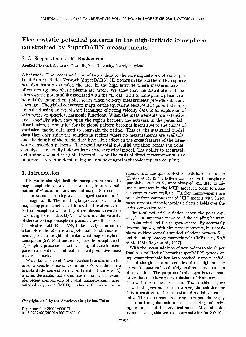
Figure 1. Locations and fields of view of the eight op- erating SuperDARN HF radars in the Northern Hemi- sphere. Flags indicate the primary source of support of each radar. Radar identification letters are defined in Table 1.

is applied to the SuperDARN data in combination with a wide variety of statistical model patterns. The lack of any significant differences in the resulting solutions of ß demonstrates that ß and hence •pc are largely constrained by the measurements alone.

3.1. Example of Fitting Technique

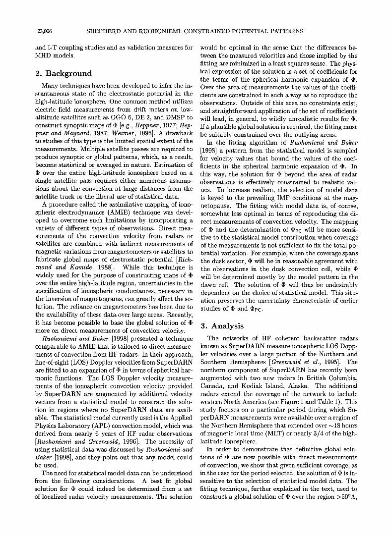
Figure 2 shows the LOS velocity data from all seven operational SuperDARN radars in the Northern Hemi- sphere during a standard 2 min scan from 1924 to 1926 UT on January 12, 2000. This period occurred before the Prince George radar was operational. The LOS

data from each radar have been mapped into a grid of geomagnetic coordinates described by Ruohoniemi and Baker [1998]. Each grid cell containing data shows the average velocity for each radar contributing to the cell. The velocity magnitude is represented by the gray level of the dot that marks the cell location, and the direc- tion is indicated by a tail on the dot that points in the direction of the observed flow. LOS Doppler measure- ments for this period are observed at >60øA and from •0700 to 2400 MLT, encompassing roughly 3/4 of the convection zone.

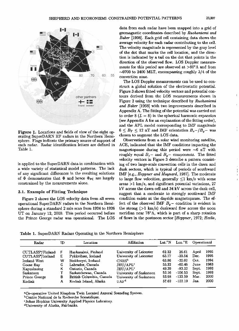
The LOS Doppler measurements can be used to con- struct a global solution of the electrostatic potential. Figure 3 shows fitted velocity vectors and potential con- tours derived from the LOS measurements shown in

Figure 2 using the technique described by Ruohoniemi and Baker [1998] with two improvements described in Appendix A. The fitting of the potential was carried out to order 8 (L - 8) in the spherical harmonic expansion (see Appendix A for an explanation of the fitting order), and the APL model corresponding to IMF magnitude 6 _< BT _< 12 nT and IMF orientation Bz-/By- was chosen to augment the LOS data.

Observations from a solar wind monitoring satellite, ACE, indicated that the IMF conditions impacting the magnetopause during this period were •6 nT with roughly equal Bz- and By-- components. The fitted velocity vectors in Figure 3 describe a pattern consist- ing of two large-scale convection cells in the dawn and dusk sectors, which is typical of periods of southward IMF [e.g., Heppner and Maynard, 1987]. The moderate to large flow velocities, generally <_1 km/s with some areas > 1 km/s, and significant potential variations, 27 kV across the dawn cell and 34 kV across the dusk cell, suggest that a moderate to strongly southward IMF condition exists at the dayside magnetopause. The ef- fect of the observed IMF By-- condition is evident in the strong (>1 km/s) duskward flow across the noon meridian near 78øA, which is part of a sharp rotation of flows in the postnoon sector [Heppner, 1972; Heelis,

Table 1. SuperDARN Radars Operating in the Northern Hemisphere

Radar ID Location Affiliation Lat.øN Lon.øE Operational

CUTLASSa/Finland F Hankasalmi, Finland University of Leicester CUTLASSa/Iceland E Pykkvibmr, Iceland University of Leicester Iceland West W Stokkseyri, Iceland CNRS b Goose Bay G Labrador, Canada JHU/APL ½ Kapuskasing K Ontario, Canada JHU/APL ½ Saskatoon T Saskatchewan, Canada University of Saskatoon Prince George B British Columbia, Canada University of Saskatoon Kodiak A Kodiak Island, Alaska UAF d

62.32 26.61 April 1995 63.77 -20.54 Dec. 1995

63.86 -20.02 Oct. 1994 53.32 -60.46 June 1983

49.39 -83.32 Sept. 1993 52.16 -106.53 Sept. 1993 53.98 -122.59 Mar. 2000

57.62 -152.19 Jan. 2000

•Co-operative United Kingdom Twin Located Auroral Sounding System. bCentre National de la Recherche Scientifique. c Johns Hopkins University Applied Physics Labratory. dUniversity of Alaska, Fairbanks.

23,008 SHEPHERD AND RUOHONIEMI: CONSTRAINED POTENTIAL PATTERNS

January 12,2000 LOS Velocity %000 m/s vel (m/s) 1924:00 - 1926:00 UT . \ 121MLT T / ,

1000

..\ K / ' 750 ß -% 5oo

x / 250

,,, C --"" . .; •.•--•.'•o• - ' .2-. A

, ,••.' "•_ • .•

,' ' '"ø ' ,, ' o 00 .•,'o• ":ooo i• . •,6M.LT

i ,oO ooO,, o ,

oo ' . ' ½,• i •^o W• . O..ooo, o • _., . ....E• ",%% o-e •', ,•.-•-•,,•,• 'o "

, /i

x x '. p. , ...• ,•2½•7• o ,

', o- •.,•'œ.•.• , x o o_ --_..e,,•.•-"' o

_ •, o_Uo • o / / 0 /

F•.6 o o % 65"A . ' --.

/ -O•œT- \

Figure 2. Line-of-sight (LOS) Doppler velocity data from seven SuperDARN HF radars in the Northern Hemisphere on January 12, 2000, 1924-1926 UT.

1984; Greenwald et al., 1990]. Also, the larger and more circular dawn cell as compared to the more crescent shaped dusk cell suggests an IMF By- condition [e.g., Reiff and Burch, 1985; Crooker, 1979]. The pattern is quite similar to the DE model of Heppner and Maynard [1987] for IMF By- conditions, particularly in the day- side.

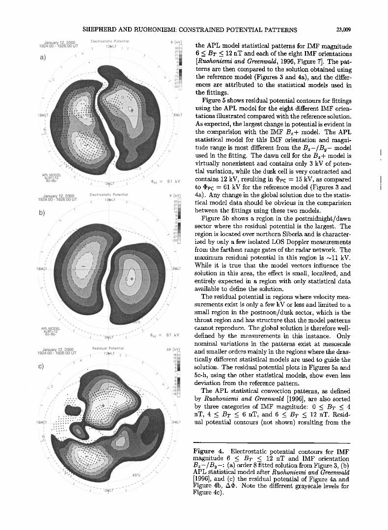
While the features of the convection pattern for this period are consistent with the IMF 6 _< Bz <_ 12 and Bz-/By- APL model, there are significant differences. Figure 4 shows grayscale shaded potential contours with dark dots marking grid cells that contain LOS measure- ments. The fitted pattern from Figure 3 is reproduced in Figure 4a for comparison with the statistical model data shown in Figure 4b.

The convection patterns in Figures 4a and 4b are sim- ilar in the largest-scale features, the two-cell morphol- ogy, and •PC. Potential variations in the dawn and dusk cells are 27 kV and -34 kV (•Pc - 61 kV), respectively, for the fitted patterns and -33 kV and 28 kV (•Pc - 61 kV), respectively, for the statistical model data. Sev- eral interesting differences exist between these potential patterns. The largest difference in the patterns occurs in the dayside, where the throat region, located in the prenoon sector of the statistical data, is rotated to the postnoon sector in the fitted solution. The resulting dawn cell in the fitted solution extends much farther

into the dusk region (-•1500 MLT) than the statistical model data predicts. In addition, the dusk cell of the fitted pattern has two regions of large negative potential that extend over a broader range of MLT than shown in the statistical pattern.

Figure 4c shows the residual potential, which we de- fine as the difference in the potential shown in Figures 4a and 4b, in this case the change from the statistical pattern to the fitted pattern. Note that the grayscale levels used in all of the residual potential plots are dif- ferent by a factor of 2 from those used in the plot of the potential solutions to dramatize changes or lack thereof. The residual potential in Figure 4c shows that the largest differences between the two patterns occur in a region of the dayside between the MLTs where the throat is located in the two patterns and the premid- night sector, into which the dusk cell of the fitted pat- tern extends. The existence of large residuals (-•35 kV) demonstrates that the LOS Doppler measurements de- termine the solution in these regions.

Smaller-scale features present in the fitted pattern (Figure 4a) but absent from the statistical model (Fig- ure 4b) are due in part to the lower-order (6) fit used by Ruohoniemi and Greenwald [1996] in constructing the statistical patterns and to the tendency of statistical constructions to supress finer-scale features.

3.2. Sensitivity to Model Choices

The purpose of this study is to demonstrate that dur- ing periods when SuperDARN velocity measurements are available over a large portion of the convection zone the particular choice of statistical model has lit- tle effect on the resulting global potential pattern. By way of example, we perform the fitting technique using

January 12,2000 Fitted Velocity •000 m/s vel (m/s) 1924:00 - 1926:00 UT 1214LT \ T /

K 1000 \ / 750

o 500

x / -- --' • • / 250

/

Bz-/By- • .... •EF - - - • •Pc = 61 kV

Figure 3. Fitted velocity vectors and electrostatic po- tential contours from the LOS measurements in Figure 2 using the technique described by Ruohoniemi and Baker [1998] to order 8 with the APL model for IMF magni- tude 6 _• Bz _• 12 nT, IMF orientation Bz-/By-, and the improvements discussed in Appendix A.

SHEPHERD AND RUOHONIEMI: CONSTRAINED POTENTIAL PATTERNS 23,009

January 12.2000 Electrostatic Potential 4, (k•

1924:00- 1926:00 UT .. \. 12MLI "T' '/ -- 33::• .

27 .......

- 21'-' 15

.q.'O .",' ' ' - •"L A -15 .;• "-27 '•33 .' ;, .. -'.-. •,•.:.:? ,. z.-,,

...... .• / . .-• •;,•:•;..-½:•::½.:..:.:•:..:•: ., . ....

: / : • ß . ½ ........ •...•;;:i'" ß ,;• ß • .... •'"'•'"'•'*••••••:••••44 •,::

. • . ,•..•:.•:•..-.:..•,.. •-:: . - •, -.,

'E -'%•' . t .• ..... . • .... •:..

. ,• ....... •:[•. ,-:.-•.,, ..,: ,. ß

""/ "..

APL MODEL 6<BT<12 "-/ -.. _ _ - •X - Bz-/By- - - - • - • •Pc -- 61 kV ...,. ._,

January 12, 2000 1924:00 - 1926:00 UT

b) ß

ß

,.,• ß

,

ß

... .. ,,,

.. ß

,.

., ß

: ß

ß

1 aM l•f.... ß

..

ß \

ß

./ ,,

.. ,,

APL MODEL 6<BT<12 "'•: Bz-/By-

Electrostatic Potential

\ 1 21M LT "/ .... 33 .....•

21

3

-15

"--27

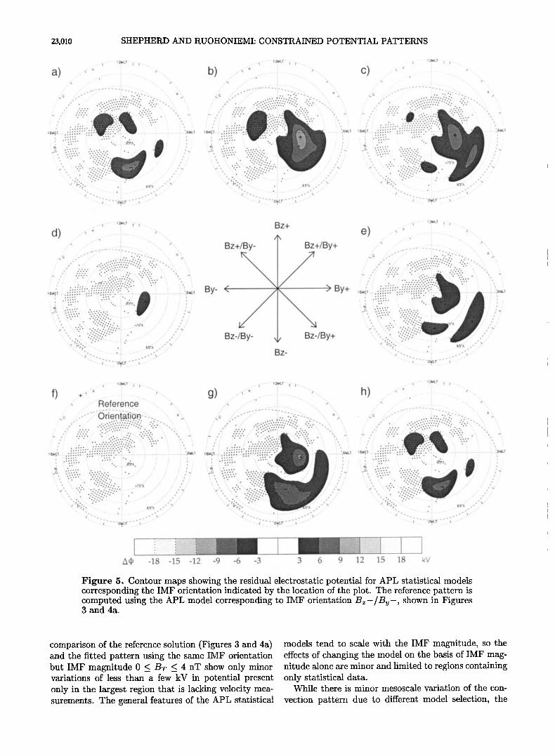
the APL model statistical patterns for IMF magnitude 6 _< Br _< 12 nT and each of the eight IMF orientations [Ruohoniemi and Greenwald, 1996, Figure 7]. The pat- terns are then compared to the solution obtained using the reference model (Figures 3 and 4a), and the differ- ences are attributed to the statistical models used in

the fittings. Figure 5 shows residual potential contours for fittings

using the APL model for the eight different IMF orien- tations illustrated compared with the reference solution. As expected, the largest change in potential is evident in the comparision with the IMF Bz+ model. The APL statistical model for this IMF orientation and magni- tude range is most different from the Bz-/By- model used in the fitting. The dawn cell for the Bz+ model is virtually nonexistent and contains only 3 kV of poten- tial variation, while the dusk cell is very contracted and contains 12 kV, resulting in •c - 15 kV, as compared to •c - 61 kV for the reference model (Figures 3 and 4a). Any change in the global solution due to the statis- tical model data should be obvious in the comparision between the fittings using these two models.

Figure 5b shows a region in the postmidnight/dawn sector where the residual potential is the largest. The region is located over northern Siberia and is character- ized by only a few isolated LOS Doppler measurements from the farthest range gates of the radar network. The maximum residual potential in this region is •11 kV. While it is true that the model vectors influence the

solution in this area, the effect is small, localized, and entirely expected in a region with only statistical data available to define the solution.

The residual potential in regions where velocity mea- surements exist is only a few kV or less and limited to a small region in the postnoon/dusk sector, which is the throat region and has structure that the model patterns cannot reproduce. The global solution is therefore well- defined by the measurements in this instance. Only nominal variations in the patterns exist at mesoscale and smaller orders mainly in the regions where the dras- tically different statistical models are used to guide the solution. The residual potential plots in Figures 5a and 5c-h, using the other statistical models, show even less deviation from the reference pattern.

The APL statistical convection patterns, as defined by Ruohoniemi and Greenwald [1996], are also sorted by three categories of IMF magnitude: 0 _< Br _< 4 nT, 4 _< Br _< 6 nT, and 6 _< Br _< 12 nT. Resid- ual potential contours (not shown) resulting from the

Figure 4. Electrostatic potential contours for IMF magnitude 6 < Br _< 12 nT and IMF orientation Bz-/By-' (a) order 8 fitted solution from Figure 3, (b) APL statistical model after Ruohoniemi and Greenwald [1996], and (c) the residual potential of Figure 4a and Figure 4b, A•. Note the different grayscale levels for Figure 4c).

23,010 SHEPHERD AND RUOHONIEMI: CONSTRAINED POTENTIAL PATTERNS

121,,ILT - -- x . I I-

., -..

(o ..;... :: .. -. '.'-•-..

• .

,.., .... .":';!.; i:' ... ß . '.-•..i.. •^

'5, ,•,-.': .::,:.%½:... •... ..

-• -•(:...

121•LT 1 21•ILT ..• : • i--- • . i i ß

b) • : ) .\ /.. C •' '< / ß

..'• ... •'. -- '-- .... .•- :;.-.•7':: ,. ,,"'.; •.• . . - ' •..- :':.-.•":'< "'.

,,,,½ ..... .:.i.?..'•:.,.';:.: ' ";':'?;'"" :'-½',-'"'" '"': ........... • ..... !'" :!i(":-'""::': ..... :::J,:.:f:"i:'""..::..L-•'",.. ' • ,, ..::.:.:::... .:,:; '.: .;: :r• .;., .... ß ': • ..:: .... ... ..... :,,::•....:, ', ; ½, ' -"•. ' "-.. '"'" '-:' 7• ':"': ; ', " .... ' : .. i'•.7g , ::' '-. '

'>El '.% .... .'. - ".". - ß : ' ß •.,: ...... ' ..' • / •' ,

•' ' '." '"-;";•'•'." '•..... ! -75'^ ';- ' ,,',•. ,

,

ß

,

'<. FL. :." .. .: 65';• . -'" ' "' •":" ' 65'^ . -' ' "" ., -.. -: __- ,.. ;•--.. --:: __.-•

.; .... o•---; ..,- -o•

121•LT ---• : f"l ß

.

ß . ..

-.. ..

.•. o , - :.. ß, ";- -'::%

... ::::::::::::::::::::::::::::::::::::: .:.':-:-- .. .. z ...- --

.:.-' ,?' . •- ;.. , '-.. ..... :,.':•;. '-"- ,'.." •, • -...

• • .. . .- ß

•, •%..-. .t....'..- .... . -' ' •

•........• ..'• . ,l/ .¾'

"< ';•'." ' • ' •s'• ..." y' -.. , • . ....... / ' ' -. _ • _ _ - '

........... ; .... •t(.---;

Bz+ . • 12MLT l: t e) ," • '•-

: . ß

Bz+ +/By+ -- ß . :.. ß... _ •-•..;..:... " . . . .. ...!.?.:?.,:.:,:::: ..:..........

By- < > By+ ' • ' ":" ':::"":'"" ...... .w• : ß ....

'•F, :•: -" •;•/j/•..j•,!i!ii• ' i ". Bz-/By- • Bz-/By+ ',:..'..'.' i -; "'

"/- •'--'." 4 ß

Bz- -., --._ 'i ..--., --'

--- ' 121•LT- ' . • - -. 121•LT' T i ..•. 121dLT l: "1 • : T I ' .-

f) +.•--• ,.. g) --•-..• ,... ,.• ,. _.

ß . ..;

* "Reference " " . i.. % <' * .... .......... -_ •' •::• _- .......... . ......... _ ....... •'•!• _'•_

•-';• .... ;-- 'Orient&fi-on.-':'<. ;"";. ' . ---:-' ......... " ..... :': ......... ;'"' •"• ..' -"- -' ' -;-'-'" ;" •.c ....' -' i.. -.'. --'_ '-.

:,i::::;.; '" ,: ?. -...

'•F--:--,-:-::::::•'!:-:-: ...... ::-:-:::->--:.i .... ;' . ........................ •,•_, ..... ,,Wt.__; ...... •.:':.::.:_::.,.;;;...':;..:..:._:..::•:L'.:.'•' .":½';..'J.:'i•?.:/:..-i.. ..... .:....'.:'.::' ........ :_._:,•-• ,,,i t ...... ,-:i-E-:"!-!-,.-i-!-: ";:'"":"."'; ..... i .......... , :: :::::: : ..... •:•. .... •s:•::...•,iiii,i;.{r½•;•....... . , ' "- ....... .. i ½•;^ I :'" -""- • ½&^. :.. ,

ß , :.. •, :....-'. •,.. .. -... -----..-- . . ,.- , . t ½, :..'.' .... • .- ß ½, '- -' .... "- ' 'i .... , <-' ">E, ':;;;..' Z.- -.'. :.., :: . . .... , < '._e, :;; .... '-'.. '.'. •-.• i ß . -" . .." ß ,'

": ....... li:i:i:':': ß ::: ':"' "" ,' ,' .: ":'"'"'-... -- "•'• ' ' '.- " ..;', .... '.':'-"......::-:':':'7": •,i!.,':½•?'"';J •'""•"' ' ....... i:' ':" z . ,

,

ß .. .•. . ,- \...- ........ •:.. ....... ß ' .•'•:'.z/.:-•:•.:.'::'.:" ...-' ,' v" -.'. r..-. s •.•' .' --<-p.:..-- .. :: ß .•.•- .-' ..y . ...... . . .. . ..:. ..•.^ ,- . . • ß

.:.'..--,, : _--" • ...... -_, --:: ....... __, ,..- ..... .•-, .... -- ,.. -..; .... o½•---, ..... --o•-.; :.- -;.----o,•,----.; .-

Figure 5. Contour maps showing the residual electrostatic potential for APL statistical models corresponding the IMF orientation indicated by the location of the plot. The reference pattern is computed using the APL model corresponding to IMF orientation Bz-/By-, shown in Figures 3 and 4a.

comparison of the reference solution (Figures 3 and 4a) and the fitted pattern using the same IMF orientation but IMF magnitude 0 <_ BT <_ 4 nT show only minor variations of less than a few kV in potential present only in the largest region that is lacking velocity mea- surements. The general features of the APL statistical

models tend to scale with the IMF magnitude, so the effects of changing the model on the basis of IMF mag- nitude alone are minor and limited to regions containing only statistical data.

While there is minor mesoscale variation of the con-

vection pattern due to different model selection, the

SHEPHERD AND RUOHONIEMI: CONSTRAINED POTENTIAL PATTERNS 23,011

total potential variation across the polar cap, (•PC, is remarkably constant regardless of the chosen statistical model. The range of •PC for the fitted patterns is only 56-61 kV, while •PC varies in the statistical patterns from 15 to 77 kV. Clearly, the LOS measurements dur-. ing this period adequately constrain the determination of (•PC-

It is instructive to consider the reason for the insensi-

tivity of the •PC determination to the selection of statis- tical model data. The area of observations apparently encompasses the positions of the potential extrema and the flows in the intervening region. Thus the total po- tential variation is fixed by the observation of convec- tion velocity through the polar cap. This important characteristic is reproduced by the fitting regardless of the nature of the sparse model data used to constrain the global solution. We can anticipate making definitive estimates of •PC when this condition prevails. Most often, this will be realized when observations extend across much of the dayside region, as in this case.

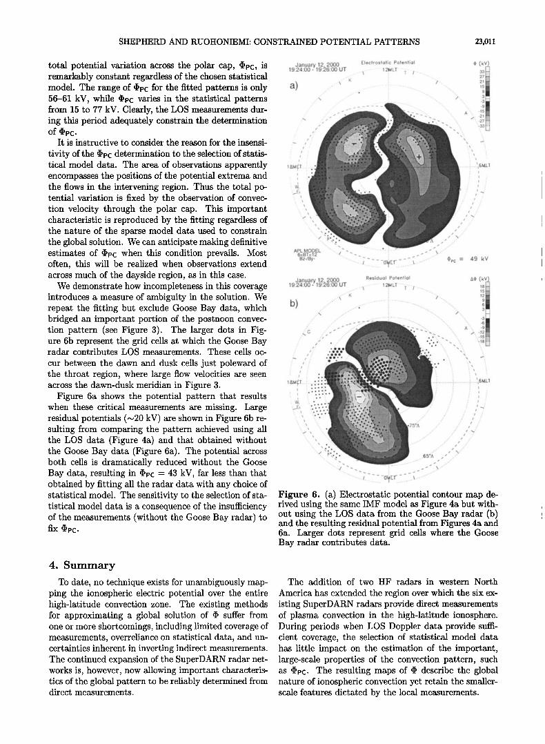
We demonstrate how incompleteness in this coverage introduces a measure of ambiguity in the solution. We repeat the fitting but exclude Goose Bay data, which bridged an important portion of the postnoon convec- tion pattern (see Figure 3). The larger dots in Fig- ure 6b represent the grid cells at which the Goose Bay radar contributes LOS measurements. These cells oc-

cur between the dawn and dusk cells just poleward of the throat region, where large flow velocities are seen across the dawn-dusk meridian in Figure 3.

Figure 6a shows the potential pattern that results when these critical measurements are missing. Large residual potentials (-•20 kV) are shown in Figure 6b re- sulting from comparing the pattern achieved using all the LOS data (Figure 4a) and that obtained without the Goose Bay data (Figure 6a). The potential across both cells is dramatically reduced without the Goose Bay data, resulting in •PC - 43 kV, far less than that obtained by fitting all the radar data with any choice of statistical model. The sensitivity to the selection of sta- tistical model data is a consequence of the insufficiency of the measurements (without the Goose Bay radar) to fix (•PC-

January 12 2000 Electrostatic Potential • (kV) 19-24-00- 19-;•6'00 UT --- -" 12MLT ..... -

.... ..--'\ : T /-'-

•/-. 21• a) -- . -_ -.

ß < . i ..... ' .... • ...... .• .'"" . '.. •.. .. •,. •; . -.' ß - -'• . '-. • -21 .... /.• .. ' ..... . •, .. ß . . .:. • • . ;'.. • • ".. '. -27 :-,-:.

. •... ...,, •,••.• . .•/:•• ..... , .. .

,•,,,•: ß ' ::"• T - : ';-- .. ':'• '• • •t .... :'.?'*•;••; •. ' ß . ß ..- :..•

i :'• '/:' '•" ..... " "•: •:• ,.d•,1,: -

. E, '"• :•:'• .... %: ..... "' ' .... '"•* '*:;•:' •-::;• ' ...... • , •;•; • ' .....:.,-:..:..:..: ....... A•;•;,,•c:•.• .... 8•. , ..- ß .. • ..• •::• ,;•:':'• Eta:... '. ":.•:.:...•? .: ,;•,.' .. / ß - • •:• ., •:::•.•-• ....... .•i:: :•:•:½•!•:•.:•, :½'. .' / -. , ' '%½ -•.. •'V.': :':'•,•½•.•'•:•½' ..- ' . ' , '. ..... •: ': :.;:•D•?•-,%- . '

ß ,,/ E. ß ........................... ::•i:;:½:;•t..•... / •.. -. r•.:. : ' ........ •:':'" - A ,' .."

,•L MOO•L ....... •'- .............. :: ....... ','. ' 6<BT<12 '-L. • • • • _ • • .-•"

•-'•' ....... 7 .... R•T---; .......... •o = 49 •v

Januar 12 2000 Residual Potential A½ (k• 19:24:00-Y19:•6:00 UT \.-. -' 12MLT .... :I: .... / 158 ....... i• i .... .,.

b) ....... ' ..... '" - .... '"" .....

•, O ..' - ' ' : ........... ' ...... : .... "' '' - -':, ". ,• -.12 ß .-;' .-" {:.. '." ::-:;• ß . ;"..-, ".. ".. 45

-:; ." ß ':.": ' '•:'::• ß ' ;'. " ". '-18

/... ß..• ß ß ' ..:. .... -,. - .... , /. o.j ß ß - -_..,. ., x ..

ß '"" '" il" ..... " '"' " : ," /1t•• :½"'•"•::' :"• " , ß .. .... •:! .½ "'"-:'•"•e•'iii '"' •.•/ ' ".

' ' '::::: :';:?'• ;.'•• '" i.."."':!': :: ......i • ' ß W• '. .. o'.. ß .•.E• .'.: ß ß ..'" / --- " • "' • ' '- ';•' ." / .:

\\ ".. , •;•.• ..' I I ,," '. • -.. ß • 75",• ...'"' / ..'

ß ' -. ,, ,• .- ,65"• "" / N ß --./ "-.__ ' ...... ! .... ,,_- \.

..... ,..;---o?•r -, ..........

Figure 6. (a) Electrostatic potential contour map de- rived using the same IMF model as Figure 4a but with- out using the LOS data from the Goose Bay radar (b) and the resulting residual potential from Figures 4a and 6a. Larger dots represent grid cells where the Goose Bay radar contributes data.

4. Summary

To date, no technique exists for unambiguously map- ping the ionospheric electric potential over the entire high-latitude convection zone. The existing methods for approximating a global solution of ß suffer from one or more shortcomings, including limited coverage of measurements, overreliance on statistical data, and un- certainties inherent in inverting indirect measurements. The continued expansion of the SuperDARN radar net- works is, however, now allowing important characteris- tics of the global pattern to be reliably determined from direct measurements.

The addition of two HF radars in western North

America has extended the region over which the six ex- isting SuperDARN radars provide direct measurements of plasma convection in the high-latitude ionosphere. During periods when LOS Doppler data provide su•- cient coverage, the selection of statistical model data has little impact on the estimation of the important, large-scale properties of the convection pattern, such as •PC. The resulting maps of ß describe the global nature of ionospheric convection yet retain the smaller- scale features dictated by the local measurements.

23,012 SHEPHERD AND RUOHONIEMI: CONSTRAINED POTENTIAL PATTERNS

An example period chosen for the extended cover- age of radar measurements illustrates the independence of the fitted solution of ß on the statistical models.

Using the fitting technique of Ruohoniemi and Baker [1998] with two improvements discussed in Appendix A, maps of ß constructed with statistical models that differ greatly in character show only minor variations. During such periods, ß and •Pc are largely determined by the observations alone.

An important threshold has now been reached; name- ly, it is now possible to reliably map ß and deter- mine •Pc using direct measurements. During the ex- ample period only seven of the eight operational radars provided measurements of the convecting ionspheric plasma. Additional measurements from the new radar in British Columbia and another currently being con- structed in Alaska will only add further confidence to ß and •pc obtained from this fitting proceedure. The product of this analysis will provide valuable checks of ionospheric quantities derived from global magneto- spheric MHD models and concepts in SW-M-I coupling.

Appendix: Modifications of APL Global Convection Mapping Technique

Two modifications have been made to the mapping technique of Ruohoniemi and Baker [1998]. The fitted convection patterns now produced by the APL group, including those presented in this paper, incorporate these modifications unless otherwise specified. Here we describe the changes and the reasons for adopting them.

The first concerns the specification of the equator- ward boundary of the convection zone. In Ruohoniemi and Baker [1998] this boundary, referred to here as A circ, was taken to be a circle of constant invariant latitude. We use the value of A circ at midnight MLT, A[ i•c - ACi•C(0000 MLT), to identify this circular bound- ary. The actual value of A[ itc was either set to a con- stant (usually 60 ø ) or varied from scan to scan to ac- commodate the varying size of the convection zone. The equatorward boundary was specified as a circle in the derivation of the statistical convection model of Ruo-

honiemi and Greenwald [1996], and this has been the accepted convention in studies of this kind. However, we have found that the SuperDARN data invariably in- dicate that the convection boundary is located at higher latitudes on the dayside than on the nightside. The defi- nition of the boundary used in the fitting should reflect this character. As a practical matter, we have found that using a circular boundary that accommodates the flow on the nightside allows the flow on the dayside to extend to unrealistically low latitudes.

The solution is to introduce an MLT dependence in the specification of the boundary latitude. We have explored several options for the boundary, including a global shifting of the coordinate flows so that the con- vection pattern is centered on a point 4 ø equatorward

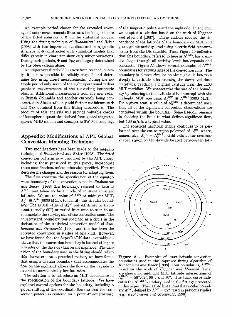
of the magnetic pole toward the nightside. In the end, we adopted a solution based on the work of Heppner and Maynard [1987]. These authors studied the de- pendence of the latitude of the boundary on MLT and geomagnetic activity level using electric field measure- ments from the DE satellite. Their Figure 10 indicates that this boundary, referred to here as A •Ms, has a sim- ilar shape through all activity levels but expands and contracts. Figure A1 shows several examples of A boundaries for varying sizes of the convection zone. The boundary is almost circular on the nightside but rises steeply in latitude after crossing the dawn and dusk meridians, reaching a highest latitude near the 1100 MLT meridian. We characterize the size of the bound-

ary by referring to the latitude of its intercept with the midnight MLT meridian, A0 •us - A•US(0000 MLT). For a given scan, a value of A0 • is determined such that all of the significant convection observations are contained within the boundary. Some freedom remains in choosing the limit to what defines significant flow, but 100 m/s is a typical value.

The spherical harmonic fitting continues to be per- formed over the entire region poleward of A•) irc, where, numerically, A•) ire - Ao HuB. Grid cells in the crescent- shaped region on the dayside located between the lati-

I \ /

Figure A1. Examples of lower-latitude convection boundaries used in the improved fitting algorithm of Ruohoniemi and Baker [1998]. Four boundaries, A based on the work of Heppner and Maynard [1987j are shown for midnight MLT latitude intersections of A0 •us - 58 ø, 62 ø, 66 ø, and 70 ø. The thick curve indi- cates the A •us boundary used in the fittings presented in this.paper. The dashed line shows the circular bound- ary A c'•, defined by A•) ir• - 62 ø, used in previous studies [e.g., Ruohoniemi and Greenwald, 1998].

SHEPHERD AND RUOHONIEMI-CONSTRAINED POTENTIAL PATTERNS 23,013

tude of A circ and A HMB (see Figure A1) are padded with zero velocity vectors. Our implementation of A HMB al- lows some small, but nonzero, potential contours to ex- ist equatorward of the HMB boundary (see, for exam- ple, Figure 3). The resulting patterns more closely re- produce the character of convection at lower latitudes.

A consequence of using the lower-latitude convection boundary defined by A HMB is a minor difference in the statistical model data used in the fitting. A careful in- spection of Figure 4b reveals subtle differences from the statistical model of Ruohoniemi and Greenwald [1996]. The patterns derived by Ruohoniemi and Greenwald [1996] were fitted using a circular lower-latitude con- vection boundary (A0) corresponding to 60øA. When the fitting technique of Ruohoniemi and Baker [1998] is used, A0 is determined by the extent of the LOS obser- vations and the statistical model is scaled accordingly, thus modifying the pattern somewhat.

The second improvement over the original fitting technique described by Ruohoniemi and Baker [1998] is a weighting scheme that reduces the tendency for the statistical model data to dominate the global solution of ß at higher-order fittings. By the order of the fitting we refer back to the expansion of ß used by Ruohoniemi and Baker [1998] in terms of spherical harmonic func- tions of order L and degree M. The values of L and M determine the resulting spatial filtering of the velocity data.

The original technique of t•nohonierni and Baker [1998] weighted the statistical model data relative to the LOS velocity data without regard to the order of the fitting. The weight assigned to a velocity value from the model was set to the geometric mean of the radar velocity measurements. Fittings at higher or- der required progressively more statistical model vec- tors (cr L 2) in order to constrain the behavior of the greater number of terms in the spherical harmonic ex- pansion over the regions of no radar observations. A fixed weighting scheme therefore causes the solution to be more influenced by the statistical data at higher or- ders. The consequence was an undesirable compromise in selecting the order of the fitting at a level high enough to adequately reproduce finer-scaled features in areas where data were present but low enough so the statis- tical model did not dominate the solution.

An improvement has been made whereby the weight of the statistical data is adjusted according to the order of the fitting. The result is that the degree to which the model vectors affect the solution is less dependent on the order of the fit. In essence, the weight defined above as the geometric mean of the radar velocity mea- surements is reduced by the factor 42/L 2. The effect is to roughly equalize the contribution of the statisti- cal model to the fitting solution for L _> 4 (fittings of order L < 4 are not considered useful). The cost asso- ciated with this progressive aleweighting might be the emergence of erratic behavior in the patterns over the areas of no radar observations. However, we have found

-• ,2•dLT I i-. -' • ' , 21•LT I I • • '-) x •< r. .... ß

.

ß .• . :: ;,.. -;, _• .... •. - . .

...._.:.- .... '--?.:_:'•:•._._• ;... -- ..:: .... : ...:•--._._

o_

•. ' .::::: .... ..- •:.•-•. •:•,:%• :;.. ,, ,;,:. :, ::. .......... , _i ,•,,:•...,.......' .... ..:;:•:'• '•-"•:½•,•.• ,,'_ , ',, ..... .:.• ':ff:.:.::5:•.. .... •;•.•-•,_•::.•.:.::. ,,,

. ..: ,.x'}',,:'.>- ' :-;.----•rr--- ;'

. .

fixed weights fitting order adjusted weights

Aq• -18 -15 -12 -9 -6 -3 3 6 9 12 15 18 kV

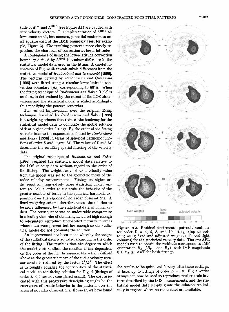
Figure A2. Residual electrostatic potential contours for order L - 4, 6, 8, and 10 fittings (top to bot- tom) using fixed and adjusted weights (left and right columns) for the statistical velocity data. The two APL models used to obtain the residuals correspond to IMF orientation B•-/B•- and B•+ with IMF magnitude 6 _< Bz _< 12 nT for both fittings.

the results to be quite satisfactory with these settings, at least up to fittings of order L = 10. Higher-order fittings can now be used to reproduce smaller-scale fea- tures described by the LOS measurements, and the sta- tistical model data simply guide the solution realisti- cally in regions where no radar data are available.

23,014 SHEPHERD AND RUOHONIEMI: CONSTRAINED POTENTIAL PATTERNS

Figure A2 shows residual potentials for varying or- ders of fit (œ = 4, 6, 8, and l0 from top to bottom) for both the fixed and varied (left and right column) weighting schemes. Inspection of the residuals in the left column of Figure A2 shows the problem of using a high-order fit with the fixed weighting scheme of Ruo- honiemi and Baker [1998]. Increasingly large (>12 kV) residual contours are evident as the order is increased.

In this example the increasing fitting order is inadver- tently causing the global solution to converge on the solution defined by the statistical model.

The right column of Figure A2 reveals a slight trend toward larger residuals with increasing fitting order, im- plying that the statistical data is influencing the so- lution to a greater extent in the higher-order fittings. However, in regions where LOS velocity data are present (e.g., 1500-1800 MLT and 75-85øA), the maximum de- viation in the residual is less than or equal to •3 kV. Such minor change in the residual contours from or- der 4 to 10 demonstrates that the improved weighting scheme allows the fitting technique to be virtually in- dependent of order in regions were velocity data are present. Larger residual deviations (up to •10 kV) are seen in the postmidnight/dawn region where no veloc- ity measurements exist. Such a trend is expected at higher orders. The additional statistical data used in the higher-order fittings cause the differences between model patterns to become more evident in locations where no data exist.

Contrasting the right column in Figure A2 with the left column shows the marked improvement the ad- justed weighting scheme has on reducing the impact of the statistical model at higher orders. Smaller-scale fea- tures present in the velocity data can now be reproduced in the global patterns without significant influence from the statistical model data.

Acknowledgments. This work was supported by NSF grant ATM-9812078 and NASA grant NAG5-8361. Oper- ation of the Northern Hemisphere SuperDARN radars is supported by the national funding agencies of the U.S., Canada, the U.K., and France. We gratefully acknowledge the CDAWeb for access to the ACE solar wind data.

Janet G. Luhmann thanks John D. Kelly and C. Robert Clauer for their assistance in evaluating this paper.

References

Boyle, C. B., P. H. Reiff, and M. R. Hairston, Empirical polar cap potentials, J. Geophys. Res., 102, 111, 1997.

Crooker, N. U., Dayside merging and cusp geometry, J. Geo- phys. Res., 8•, 951, 1979.

Greenwald, R. A., K. B. Baker, J. M. Ruohoniemi, J. R. Du- deney, M. Pinnock, N. Mattin, J. M. Leonard, and R. P. Lepping, Simulataneous observations of dynamic varia- tions in high-latitude dayside convection due to changes in IMF By, J. Geophys. Res., 95, 8057, 1990.

Greenwald, R. A., et al., DARN/SUPERDARN: A global view of the dynamics of high-latitude convection, Space Sci. Rev., 71, 761, 1995.

Heelis, Pt. A., The effects of interplanetary magnetic field orientation on dayside high latitude ionospheric convec- tion, J. Geophys. Res., 39, 2873, 1984.

Heppner, J.P., Polar-cap electric field distributions related to the interplanetary magnetic field direction, J. Geophys. Res., 77, 4877, 1972.

Heppner, J.P., Empirical-models of high-latitude electric- fields, J. Geophys. Res., 32, 1115, 1977.

Heppner, J.P., and N. C. Maynard, Empirical high-latitude electric field models, J. Geophys. Res., 92, 4467, 1987.

Pteiff, P. H., and J. L. Burch, IMF By-dependent plasma flow and Birkeland currents in the dayside magnetosphere: A global model for northward and southward IMF, J. Geo- phys. Res., 90, 1595, 1985.

Reiff, P. H., Pt. W. Spiro, and T. W. Hill, Dependence of polar cap potential drop on interplanetary parameters, J. Geophys. Res., 36, 7639, 1981.

Ptichmond, A.D., and Y. Kamide, Mapping electrodynamic features of the high-latitude ionosphere from localized ob- servations: Technique, J. Geophys. Res., 93, 5741, 1988.

Ptuohoniemi, J. M., and K. B. Baker, Large-scale imaging of high-latitude convection with Super Dual Auroral Ptadar Network HF radar observations, J. Geophys. Res., 103, 20,797, 1998.

Ptuohoniemi, J. M., and Pt. A. Greenwald, Statistical pat- terns of high-latitude convection obtained from Goose Bay HF radar observations, J. Geophys. Res., 101, 21,743, 1996.

Ruohoniemi, J. M., and R. A. Greenwald, The response of high-latitude convection to a sudden southward IMF turn- ing, Geophys. Res. Left., 25, 2913, 1998.

Slinker, S. P., J. A. Fedder, B. A. Emery, K. B. Baker, D. Lummerzheim, J. G. Lyon, and F. J. Rich, Comparison of global MHD simulations with AMIE simulations for the events of May 19-20, 1996, J. Oeophys. Res., 10•4,28,379, 1999.

Weimer, D. Pt., Models of high-latitude electric potentials derived with a least error fit of spherical harmonic func- tions, J. Geophys. Res., 100, 19,595, 1995.

J. M. Ruohoniemi and S. G. Shepherd, The Johns Hopkins University Applied Physics Laboratory, 11100 Johns Hop- kins Road, Laurel, MD 20723. (mike.ruohoniemi@jhuapl. edu; simon.shepherd@jhuapl.edu)

(Received May 11, 2000; revised July 13, 2000; accepted July 13, 2000.)