Electronic Structure Calculations with Dynamical Mean–Field Theory: A

Spectral Density Functional Approach

G. Kotliar1,6, S. Y. Savrasov2, K. Haule1,4, V. S. Oudovenko1,3, O. Parcollet5 and C.A. Marianetti1

1Department of Physics and Astronomy and Center for Condensed Matter Theory, Rutgers University, Piscataway,

NJ 08854–80192Department of Physics, University of California, Davis, CA 956163Bogoliubov Laboratory for Theoretical Physics, Joint Institute for Nuclear Research, 141980 Dubna, Russia4Jozef Stefan Institute, SI-1000 Ljubljana, Slovenia5 Service de Physique Theorique, CEA Saclay, 91191 Gif-Sur-Yvette, France and6 Centre de Physique Theorique, Ecole Polytechnique 91128 Palaiseau Cedex, France

(Dated: November 2, 2005)

We present a review of the basic ideas and techniques of the spectral density functional theorywhich are currently used in electronic structure calculations of strongly–correlated materials wherethe one–electron description breaks down. We illustrate the method with several examples whereinteractions play a dominant role: systems near metal–insulator transition, systems near volumecollapse transition, and systems with local moments.

Contents

I. Introduction 1A. Electronic structure of correlated systems 3B. The effective action formalism and the constraining

field 41. Density functional theory 62. Baym–Kadanoff functional 83. Formulation in terms of the screened interaction 94. Approximations 105. Model Hamiltonians and first principles approaches 116. Model Hamiltonians 11

II. Spectral density functional approach 13A. Functional of local Green’s function 13

1. A non–interacting reference system: bands in afrequency–dependent potential 14

2. An interacting reference system: a dressed atom 153. Construction of approximations: dynamical

mean–field theory as an approximation. 164. Cavity construction 165. Practical implementation of the self–consistency

condition in DMFT. 17B. Extension to clusters 18C. LDA+U method. 22D. LDA+DMFT theory 24E. Equations in real space 27F. Application to lattice dynamics 30G. Application to optics and transport 31

III. Techniques for solving the impurity model 33A. Perturbation expansion in Coulomb interaction 34B. Perturbation expansion in the hybridization strength 36C. Approaching the atomic limit: decoupling scheme,

Hubbard I and lowest order perturbation theory 40D. Quantum Monte Carlo: Hirsch–Fye method 41

1. A generic quantum impurity problem 422. Hirsch–Fye algorithm 43

E. Mean–field slave boson approach 48F. Interpolative schemes 49

1. Rational interpolation for the self–energy 492. Iterative perturbation theory 51

IV. Application to materials 53A. Metal–insulator transitions 53

1. Pressure driven metal–insulator transitions 53

2. Doping driven metal–insulator transition 583. Further developments 60

B. Volume collapse transitions 611. Cerium 622. Plutonium 64

C. Systems with local moments 661. Iron and Nickel 672. Classical Mott insulators 69

D. Other applications 70

V. Outlook 72

Acknowledgments 72

A. Derivations for the QMC section 73

B. Software for carrying out realistic DMFT studies. 74a. Impurity solvers 74b. Density functional theory 74c. DFT+DMFT 74d. Tight–binding cluster DMFT code (LISA) 75

C. Basics of the Baym–Kadanoff functional 751. Baym–Kadanoff functional at λ = 0 762. Baym–Kadanoff functional at λ = 1 773. Interacting part of Baym–Kadanoff functional 774. The total energy 78

References 79

I. INTRODUCTION

Theoretical understanding of the behavior of materi-als is a great intellectual challenge and may be the key tonew technologies. We now have a firm understanding ofsimple materials such as noble metals and semiconduc-tors. The conceptual basis characterizing the spectrum oflow–lying excitations in these systems is well establishedby the Landau Fermi liquid theory (Pines and Nozieres,1966). We also have quantitative techniques for comput-ing ground states properties, such as the density func-tional theory (DFT) in the local density and generalized

2

gradient approximation (LDA and GGA) (Lundqvist andMarch, 1983). These techniques also can be successfullyused as starting points for perturbative computation ofone–electron spectra, such as the GW method (Aryase-tiawan and Gunnarsson, 1998).

The scientific frontier that one would like to exploreis a category of materials which falls under the rubric ofstrongly–correlated electron systems. These are complexmaterials, with electrons occupying active 3d-, 4f - or 5f–orbitals, (and sometimes p- orbitals as in many organiccompounds and in Bucky–balls–based materials (Gun-narsson, 1997)). The excitation spectra in these systemscannot be described in terms of well–defined quasipar-ticles over a wide range of temperatures and frequen-cies. In this situation band theory concepts are not suffi-cient and new ideas such as those of Hubbard bands andnarrow coherent quasiparticle bands are needed for thedescription of the electronic structure. (Georges et al.,1996; Kotliar and Vollhardt, 2004).

Strongly correlated electron systems have frustratedinteractions, reflecting the competition between differ-ent forms of order. The tendency towards delocalizationleading to band formation and the tendency to localiza-tion leading to atomic like behavior is better describedin real space. The competition between different formsof long–range order (superconducting, stripe–like densitywaves, complex forms of frustrated non–collinear mag-netism etc.) leads to complex phase diagrams and exoticphysical properties.

Strongly correlated electron systems have many un-usual properties. They are extremely sensitive to smallchanges in their control parameters resulting in large re-sponses, tendencies to phase separation, and formationof complex patterns in chemically inhomogeneous situa-tions (Mathur and Littlewood, 2003; Millis, 2003). Thismakes their study challenging, and the prospects for ap-plications particularly exciting.

The promise of strongly–correlated materials contin-ues to be realized experimentally. High superconductingtransition temperatures (above liquid Nitrogen temper-atures) were totally unexpected. They were realized inmaterials containing Copper and Oxygen. A surprisinglylarge dielectric constant, in a wide range of tempera-ture was recently found in Mott insulator CaCu3Ti4O12

(Lixin et al., 2002). Enormous mass renormalizations arerealized in systems containing rare earth and actinide el-ements, the so–called heavy fermion systems (Stewart,2001). Their large orbital degeneracy and large effec-tive masses give exceptionally large Seebeck coefficients,and have the potential for being useful thermoelectrics inthe low–temperature region (Sales et al., 1996). Colossalmagnetoresistance, a dramatic sensitivity of the resistiv-ity to applied magnetic fields, was discovered recently(Tokura, 1990) in many materials including the proto-typical LaxSr1−xMnO3. A gigantic non–linear opticalsusceptibility with an ultrafast recovery time was discov-ered in Mott insulating chains (Ogasawara et al., 2000).

These non–comprehensive lists of remarkable materials

and their unusual physical properties are meant to illus-trate that discoveries in the areas of correlated materialsoccur serendipitously. Unfortunately, lacking the propertheoretical tools and daunted by the complexity of thematerials, there have not been success stories in predict-ing new directions for even incremental improvement ofmaterial performance using strongly–correlated systems.

In our view, this situation is likely to change in thevery near future as a result of the introduction of a prac-tical but powerful new many body method, the Dynam-ical Mean Field Theory (DMFT). This method is basedon a mapping of the full many body problem of solidstate physics onto a quantum impurity model, which isessentially a small number of quantum degrees of freedomembedded in a bath that obeys a self consistency condi-tion (Georges and Kotliar, 1992). This approach, offersa minimal description of the electronic structure of cor-related materials, treating both the Hubbard bands andthe quasiparticle bands on the same footing. It becomesexact in the limit of infinite lattice coordination intro-duced in the pioneering work of Metzner and Vollhardt(Metzner and Vollhardt, 1989).

Recent advances (Anisimov et al., 1997a; Lichtensteinand Katsnelson, 1997, 1998) have combined dynamicalmean–field theory (DMFT) (Georges et al., 1996; Kotliarand Vollhardt, 2004) with electronic structure techniques(for other DMFT reviews, see (Freericks and Zlatic, 2003;Georges, 2004a,b; Held et al., 2001c, 2003; Lichtensteinet al., 2002a; Maier et al., 2004a)) These developments,combined with increasing computational power and novelalgorithms, offer the possibility of turning DMFT into auseful method for computer aided material design involv-ing strongly correlated materials.

This review is an introduction to the rapidly develop-ing field of electronic structure calculations of strongly–correlated materials. Our primary goal is to present someconcepts and computational tools that are allowing afirst–principles description of these systems. We reviewthe work of both the many–body physics and the elec-tronic structure communities who are currently makingimportant contributions in this area. For the electronicstructure community, the DMFT approach gives accessto new regimes for which traditional methods based onextensions of DFT do not work. For the many–bodycommunity, electronic structure calculations bring sys-tem specific information needed to formulate interestingmany–body problems related to a given material.

The introductory section I discusses the importance ofab initio description in strongly–correlated solids. Wereview briefly the main concepts behind the approachesbased on model Hamiltonians and density functional the-ory to put in perspective the current techniques combin-ing DMFT with electronic structure methods. In the lastfew years, the DMFT method has reached a great degreeof generality which gives the flexibility to tackle realis-tic electronic structure problems, and we review thesedevelopments in Section II. This section describes howthe DMFT and electronic structure LDA theory can be

3

combined together. We stress the existence of new func-tionals for electronic structure calculations and reviewapplications of these developments for calculating variousproperties such as lattice dynamics, optics and transport.The heart of the dynamical mean–field description of asystem with local interactions is the quantum impuritymodel. Its solution is the bottleneck of all DMFT algo-rithms. In Section III we review various impurity solverswhich are currently in use, ranging from the formally ex-act but computationally expensive quantum Monte Carlo(QMC) method to various approximate schemes. One ofthe most important developments of the past was a fullyself–consistent implementation of the LDA+DMFT ap-proach, which sheds new light on the mysterious prop-erties of Plutonium (Savrasov et al., 2001). Section IVis devoted to three typical applications of the formal-ism: the problem of the electronic structure near a Motttransition, the problem of volume collapse transitions,and the problem of the description of systems with localmoments. We conclude our review in Section V. Sometechnical aspects of the implementations as well as thedescription of DMFT codes are provided in the onlinenotes to this review (see Appendix B).

A. Electronic structure of correlated systems

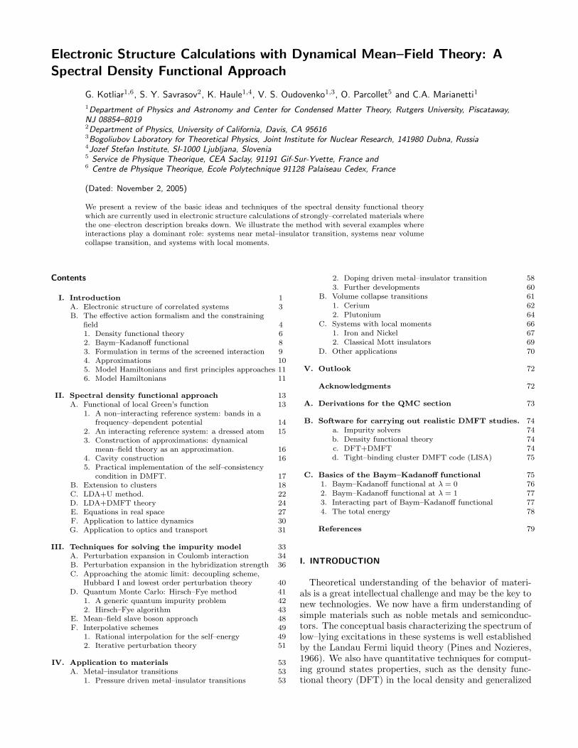
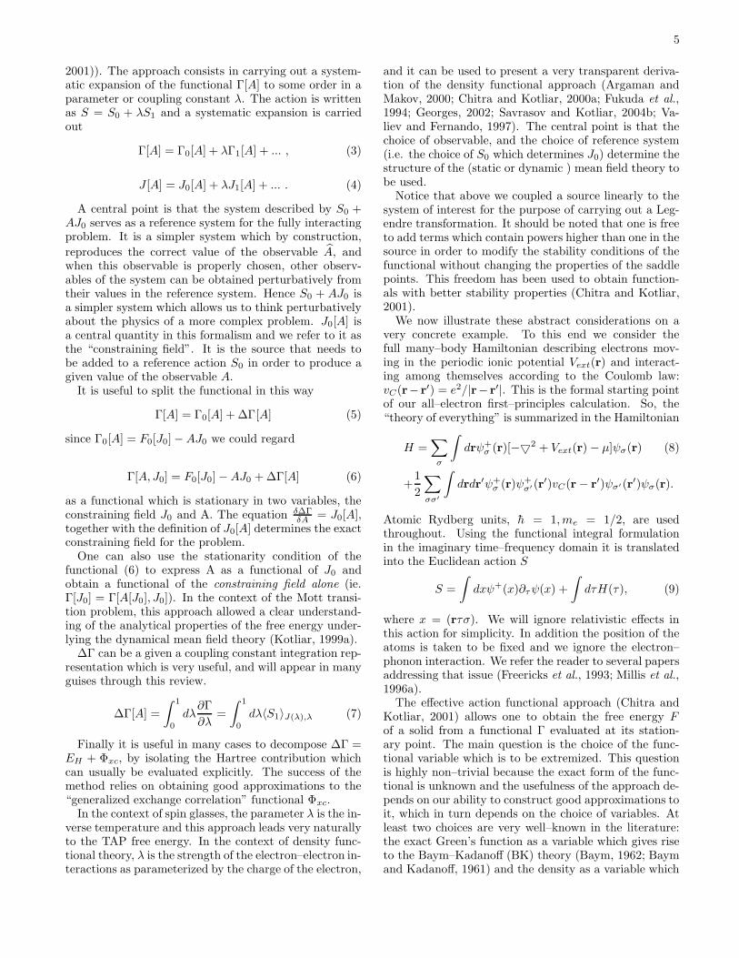
What do we mean by a strongly–correlated phe-nomenon? We can answer this question from the per-spective of electronic structure theory, where the one–electron excitations are well–defined and represented asdelta–function–like peaks showing the locations of quasi-particles at the energy scale of the electronic spectralfunctions (Fig. 1(a)). Strong correlations would mean thebreakdown of the effective one–particle description: thewave function of the system becomes essentially many–body–like, being represented by combinations of Slaterdeterminants, and the one–particle Green’s functions nolonger exhibit single peaked features (Fig. 1 (b)).

k

w

ImG(k,w)

k

w

ImG(k,w)

w

ImG(k,w)

k

e(k)

w

ImG(k,w)

k

e(k)

(a) (b)

FIG. 1 Evolution of the non-interacting spectrum (a) intothe interacting spectrum (b) as the Coulomb interaction in-creases. Panels (a) and (b) correspond to LDA-like andDMFT-like solutions, respectively.

The development of methods for studying strongly–correlated materials has a long history in condensed mat-ter physics. These efforts have traditionally focused onmodel Hamiltonians using techniques such as diagram-matic methods (Bickers and Scalapino, 1989), quantumMonte Carlo simulations (Jarrell and Gubernatis, 1996),exact diagonalization for finite–size clusters (Dagotto,1994), density matrix renormalization group methods (U.Schollwock, 2005; White, 1992) and so on. Model Hamil-tonians are usually written for a given solid–state sys-tem based on physical grounds. Development of LDA+U(Anisimov et al., 1997b) and self–interaction corrected(SIC) (Svane and Gunnarsson, 1990; Szotek et al., 1993)methods, many–body perturbative approaches based onGW and its extensions (Aryasetiawan and Gunnarsson,1998), as well as the time–dependent version of the den-sity functional theory (Gross et al., 1996) have been car-ried out by the electronic structure community. Some ofthese techniques are already much more complicated andtime–consuming compared to the standard LDA basedalgorithms, and therefore the real exploration of materi-als is frequently performed by simplified versions utilizingapproximations such as the plasmon–pole form for thedielectric function (Hybertsen and Louie, 1986), omit-ting the self–consistency within GW (Aryasetiawan andGunnarsson, 1998) or assuming locality of the GW self–energy (Zein and Antropov, 2002).

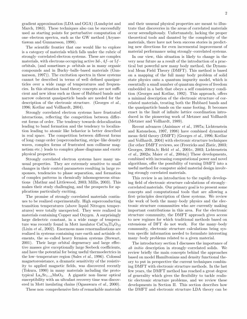
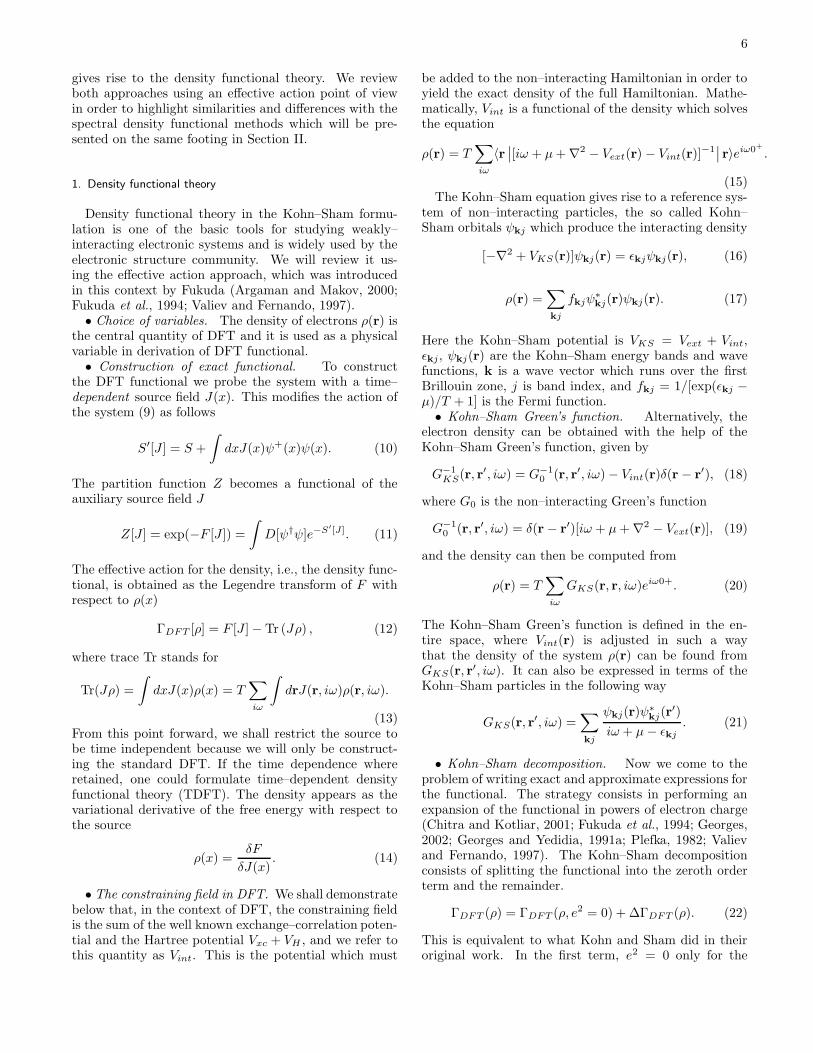
The one–electron densities of states of strongly corre-lated systems may display both renormalized quasiparti-cles and atomic–like states simultaneously (Georges andKotliar, 1992; Zhang et al., 1993). To treat them oneneeds a technique which is able to treat quasi-particlebands and Hubbard bands on the same footing, andwhich is able to interpolate between atomic and band lim-its. Dynamical mean–field theory (Georges et al., 1996)is the simplest approach which captures these features;it has been extensively developed to study model Hamil-tonians. Fig. 2 shows the development of the spectrumwhile increasing the strength of Coulomb interaction Uas obtained by DMFT solution of the Hubbard model.It illustrates the necessity to go beyond static mean–fieldtreatments in the situations when the on–site HubbardU becomes comparable with the bandwidth W .

Model Hamiltonian based DMFT methods have suc-cessfully described regimes U/W >∼ 1. Howeverto describe strongly correlated materials we need toincorporate realistic electronic structure because thelow–temperature physics of systems near localization–delocalization crossover is non–universal, system specific,and very sensitive to the lattice structure and orbital de-generacy which is unique to each compound. We believethat incorporating this information into the many–bodytreatment of this system is a necessary first step beforemore general lessons about strong–correlation phenom-ena can be drawn. In this respect, we recall that DFTin its common approximations, such as LDA or GGA,brings a system specific description into calculations. De-spite the great success of DFT for studying weakly cor-

4

2

0

2

0

2

0

2

0

2

0

-Im

G

w

-4 -2 0 2 4

U/D=1

U/D=2

U/D=2.5

U/D=3

U/D=4

/D

FIG. 2 Local spectral density at T = 0, for several values ofU , obtained by the iterated perturbation theory approxima-tion (from (Zhang et al., 1993)).

related solids, it has not been able thus far to addressstrongly–correlated phenomena. So, we see that bothdensity functional based and many–body model Hamil-tonian approaches are to a large extent complementary toeach other. One–electron Hamiltonians, which are nec-essarily generated within density functional approaches(i.e. the hopping terms), can be used as input for morechallenging many–body calculations. This path has beenundertaken in a first paper of Anisimov et al. (Anisi-mov et al., 1997a) which introduced the LDA+DMFTmethod of electronic structure for strongly–correlatedsystems and applied it to the photoemission spectrumof La1−xSrxTiO3. Near the Mott transition, this sys-tem shows a number of features incompatible with theone–electron description (Fujimori et al., 1992a). Theelectronic structure of Fe has been shown to be in betteragreement with experiment within DMFT in compari-son with LDA (Lichtenstein and Katsnelson, 1997, 1998).The photoemission spectrum near the Mott transition inV2O3 has been studied (Held et al., 2001a), as well asissues connected to the finite temperature magnetism ofFe and Ni were explored (Lichtenstein et al., 2001).

Despite these successful developments, we also wouldlike to emphasize a more ambitious goal: to build ageneral method which treats all bands and all electronson the same footing, determines both hoppings and in-teractions internally using a fully self–consistent proce-dure, and accesses both energetics and spectra of cor-related materials. These efforts have been undertakenin a series of papers (Chitra and Kotliar, 2000a, 2001)which gave us a functional description of the problem incomplete analogy to the density functional theory, andits self–consistent implementation is illustrated on Plu-tonium (Savrasov and Kotliar, 2004a; Savrasov et al.,2001).

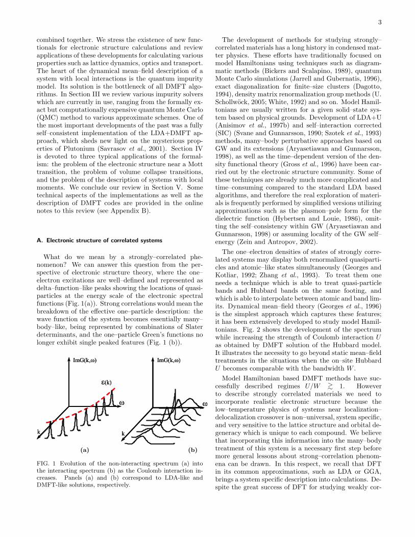
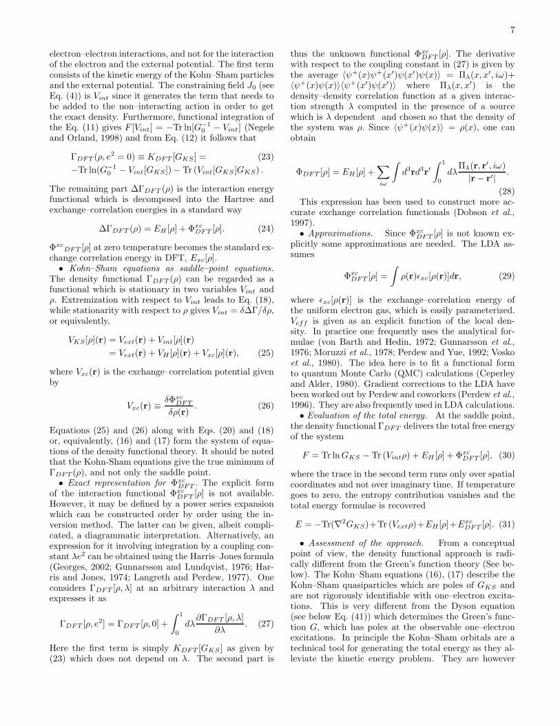
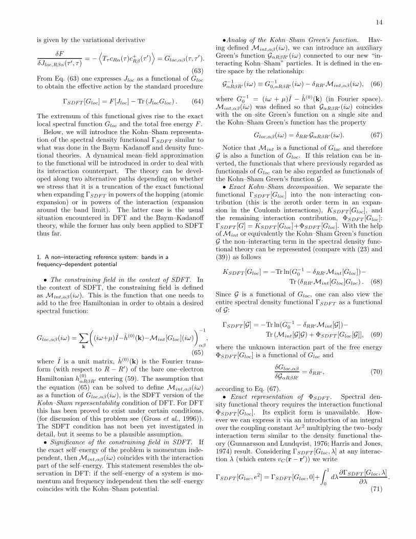
To summarize, we see the existence of two roads inapproaching the problem of simulating correlated ma-terials properties, which we illustrate in Fig. 52. To

describe these efforts in a language understandable byboth electronic structure and many–body communities,and to stress qualitative differences and great similari-ties between DMFT and LDA, we start our review withdiscussing a general many–body framework based on theeffective action approach to strongly–correlated systems(Chitra and Kotliar, 2001).

Model Hamiltonian

Correlation Functions, Total

Energies, etc.

Crystal structure +

Atomic positions

Model Hamiltonian

Correlation Functions, Total

Energies, etc.

Crystal structure +

Atomic positions

FIG. 3 Two roads in approaching the problem of simulatingcorrelated materials properties.

B. The effective action formalism and the constraining field

The effective action formalism, which utilizes func-tional Legendre transformations and the inversionmethod (for a comprehensive review see (Fukuda et al.,1995), also see online notes), allows us to present a uni-fied description of many seemingly different approachesto electronic structure. The idea is very simple, and hasbeen used in other areas such as quantum field theory andstatistical mechanics of spin systems. We begin with thefree energy of the system written as a functional integral

exp(−F ) =

∫D[ψ†ψ]e−S . (1)

where F is the free energy, S is the action for a givenHamiltonian, and ψ is a Grassmann variable (Negele andOrland, 1998). One then selects an observable quantityof interest A, and couples a source J to the observableA. This results in a modified action S + JA, and thefree energy F [J ] is now a functional of the source J . ALegendre transformation is then used to eliminate thesource in favor of the observable yielding a new functional

Γ[A] = F [J [A]] −AJ [A] (2)

Γ[A] is useful in that the variational derivative with re-spect to A yields J . We are free to set the source to zero,and thus the the extremum of Γ[A] gives the free energyof the system.

The value of the approach is that useful approxima-tions to the functional Γ[A] can be constructed in prac-tice using the inversion method, a powerful techniqueintroduced to derive the TAP (Thouless, Anderson andPalmer) equations in spin glasses by (Plefka, 1982) andby (Fukuda, 1988) to investigate chiral symmetry break-ing in QCD (see also Refs. (Fukuda et al., 1994; Georgesand Yedidia, 1991b; Opper and Winther, 2001; Yedidia,

5

2001)). The approach consists in carrying out a system-atic expansion of the functional Γ[A] to some order in aparameter or coupling constant λ. The action is writtenas S = S0 + λS1 and a systematic expansion is carriedout

Γ[A] = Γ0[A] + λΓ1[A] + ... , (3)

J [A] = J0[A] + λJ1[A] + ... . (4)

A central point is that the system described by S0 +AJ0 serves as a reference system for the fully interactingproblem. It is a simpler system which by construction,

reproduces the correct value of the observable A, andwhen this observable is properly chosen, other observ-ables of the system can be obtained perturbatively fromtheir values in the reference system. Hence S0 + AJ0 isa simpler system which allows us to think perturbativelyabout the physics of a more complex problem. J0[A] isa central quantity in this formalism and we refer to it asthe “constraining field”. It is the source that needs tobe added to a reference action S0 in order to produce agiven value of the observable A.

It is useful to split the functional in this way

Γ[A] = Γ0[A] + ∆Γ[A] (5)

since Γ0[A] = F0[J0] −AJ0 we could regard

Γ[A, J0] = F0[J0] −AJ0 + ∆Γ[A] (6)

as a functional which is stationary in two variables, theconstraining field J0 and A. The equation δ∆Γ

δA = J0[A],together with the definition of J0[A] determines the exactconstraining field for the problem.

One can also use the stationarity condition of thefunctional (6) to express A as a functional of J0 andobtain a functional of the constraining field alone (ie.Γ[J0] = Γ[A[J0], J0]). In the context of the Mott transi-tion problem, this approach allowed a clear understand-ing of the analytical properties of the free energy under-lying the dynamical mean field theory (Kotliar, 1999a).

∆Γ can be a given a coupling constant integration rep-resentation which is very useful, and will appear in manyguises through this review.

∆Γ[A] =

∫ 1

0

dλ∂Γ

∂λ=

∫ 1

0

dλ〈S1〉J(λ),λ (7)

Finally it is useful in many cases to decompose ∆Γ =EH + Φxc, by isolating the Hartree contribution whichcan usually be evaluated explicitly. The success of themethod relies on obtaining good approximations to the“generalized exchange correlation” functional Φxc.

In the context of spin glasses, the parameter λ is the in-verse temperature and this approach leads very naturallyto the TAP free energy. In the context of density func-tional theory, λ is the strength of the electron–electron in-teractions as parameterized by the charge of the electron,

and it can be used to present a very transparent deriva-tion of the density functional approach (Argaman andMakov, 2000; Chitra and Kotliar, 2000a; Fukuda et al.,1994; Georges, 2002; Savrasov and Kotliar, 2004b; Va-liev and Fernando, 1997). The central point is that thechoice of observable, and the choice of reference system(i.e. the choice of S0 which determines J0) determine thestructure of the (static or dynamic ) mean field theory tobe used.

Notice that above we coupled a source linearly to thesystem of interest for the purpose of carrying out a Leg-endre transformation. It should be noted that one is freeto add terms which contain powers higher than one in thesource in order to modify the stability conditions of thefunctional without changing the properties of the saddlepoints. This freedom has been used to obtain function-als with better stability properties (Chitra and Kotliar,2001).

We now illustrate these abstract considerations on avery concrete example. To this end we consider thefull many–body Hamiltonian describing electrons mov-ing in the periodic ionic potential Vext(r) and interact-ing among themselves according to the Coulomb law:vC(r− r′) = e2/|r− r′|. This is the formal starting pointof our all–electron first–principles calculation. So, the“theory of everything” is summarized in the Hamiltonian

H =∑

σ

∫drψ+

σ (r)[−52 + Vext(r) − µ]ψσ(r) (8)

+1

2

∑

σσ′

∫drdr′ψ+

σ (r)ψ+σ′ (r

′)vC(r − r′)ψσ′ (r′)ψσ(r).

Atomic Rydberg units, h = 1,me = 1/2, are usedthroughout. Using the functional integral formulationin the imaginary time–frequency domain it is translatedinto the Euclidean action S

S =

∫dxψ+(x)∂τψ(x) +

∫dτH(τ), (9)

where x = (rτσ). We will ignore relativistic effects inthis action for simplicity. In addition the position of theatoms is taken to be fixed and we ignore the electron–phonon interaction. We refer the reader to several papersaddressing that issue (Freericks et al., 1993; Millis et al.,1996a).

The effective action functional approach (Chitra andKotliar, 2001) allows one to obtain the free energy Fof a solid from a functional Γ evaluated at its station-ary point. The main question is the choice of the func-tional variable which is to be extremized. This questionis highly non–trivial because the exact form of the func-tional is unknown and the usefulness of the approach de-pends on our ability to construct good approximations toit, which in turn depends on the choice of variables. Atleast two choices are very well–known in the literature:the exact Green’s function as a variable which gives riseto the Baym–Kadanoff (BK) theory (Baym, 1962; Baymand Kadanoff, 1961) and the density as a variable which

6

gives rise to the density functional theory. We reviewboth approaches using an effective action point of viewin order to highlight similarities and differences with thespectral density functional methods which will be pre-sented on the same footing in Section II.

1. Density functional theory

Density functional theory in the Kohn–Sham formu-lation is one of the basic tools for studying weakly–interacting electronic systems and is widely used by theelectronic structure community. We will review it us-ing the effective action approach, which was introducedin this context by Fukuda (Argaman and Makov, 2000;Fukuda et al., 1994; Valiev and Fernando, 1997).• Choice of variables. The density of electrons ρ(r) is

the central quantity of DFT and it is used as a physicalvariable in derivation of DFT functional.• Construction of exact functional. To construct

the DFT functional we probe the system with a time–dependent source field J(x). This modifies the action ofthe system (9) as follows

S′[J ] = S +

∫dxJ(x)ψ+(x)ψ(x). (10)

The partition function Z becomes a functional of theauxiliary source field J

Z[J ] = exp(−F [J ]) =

∫D[ψ†ψ]e−S′[J]. (11)

The effective action for the density, i.e., the density func-tional, is obtained as the Legendre transform of F withrespect to ρ(x)

ΓDFT [ρ] = F [J ] − Tr (Jρ) , (12)

where trace Tr stands for

Tr(Jρ) =

∫dxJ(x)ρ(x) = T

∑

iω

∫drJ(r, iω)ρ(r, iω).

(13)From this point forward, we shall restrict the source tobe time independent because we will only be construct-ing the standard DFT. If the time dependence whereretained, one could formulate time–dependent densityfunctional theory (TDFT). The density appears as thevariational derivative of the free energy with respect tothe source

ρ(x) =δF

δJ(x). (14)

• The constraining field in DFT. We shall demonstratebelow that, in the context of DFT, the constraining fieldis the sum of the well known exchange–correlation poten-tial and the Hartree potential Vxc + VH , and we refer tothis quantity as Vint. This is the potential which must

be added to the non–interacting Hamiltonian in order toyield the exact density of the full Hamiltonian. Mathe-matically, Vint is a functional of the density which solvesthe equation

ρ(r) = T∑

iω

〈r∣∣[iω + µ+ ∇2 − Vext(r) − Vint(r)]

−1∣∣ r〉eiω0+

.

(15)The Kohn–Sham equation gives rise to a reference sys-

tem of non–interacting particles, the so called Kohn–Sham orbitals ψkj which produce the interacting density

[−∇2 + VKS(r)]ψkj(r) = εkjψkj(r), (16)

ρ(r) =∑

kj

fkjψ∗kj(r)ψkj(r). (17)

Here the Kohn–Sham potential is VKS = Vext + Vint,εkj , ψkj(r) are the Kohn–Sham energy bands and wavefunctions, k is a wave vector which runs over the firstBrillouin zone, j is band index, and fkj = 1/[exp(εkj −µ)/T + 1] is the Fermi function.• Kohn–Sham Green’s function. Alternatively, the

electron density can be obtained with the help of theKohn–Sham Green’s function, given by

G−1KS(r, r′, iω) = G−1

0 (r, r′, iω) − Vint(r)δ(r − r′), (18)

where G0 is the non–interacting Green’s function

G−10 (r, r′, iω) = δ(r − r′)[iω + µ+ ∇2 − Vext(r)], (19)

and the density can then be computed from

ρ(r) = T∑

iω

GKS(r, r, iω)eiω0+. (20)

The Kohn–Sham Green’s function is defined in the en-tire space, where Vint(r) is adjusted in such a waythat the density of the system ρ(r) can be found fromGKS(r, r′, iω). It can also be expressed in terms of theKohn–Sham particles in the following way

GKS(r, r′, iω) =∑

kj

ψkj(r)ψ∗kj(r

′)

iω + µ− εkj. (21)

• Kohn–Sham decomposition. Now we come to theproblem of writing exact and approximate expressions forthe functional. The strategy consists in performing anexpansion of the functional in powers of electron charge(Chitra and Kotliar, 2001; Fukuda et al., 1994; Georges,2002; Georges and Yedidia, 1991a; Plefka, 1982; Valievand Fernando, 1997). The Kohn–Sham decompositionconsists of splitting the functional into the zeroth orderterm and the remainder.

ΓDFT (ρ) = ΓDFT (ρ, e2 = 0) + ∆ΓDFT (ρ). (22)

This is equivalent to what Kohn and Sham did in theiroriginal work. In the first term, e2 = 0 only for the

7

electron–electron interactions, and not for the interactionof the electron and the external potential. The first termconsists of the kinetic energy of the Kohn–Sham particlesand the external potential. The constraining field J0 (seeEq. (4)) is Vint since it generates the term that needs tobe added to the non–interacting action in order to getthe exact density. Furthermore, functional integration ofthe Eq. (11) gives F [Vint] = −Tr ln[G−1

0 − Vint] (Negeleand Orland, 1998) and from Eq. (12) it follows that

ΓDFT (ρ, e2 = 0) ≡ KDFT [GKS ] = (23)

−Tr ln(G−10 − Vint[GKS ]) − Tr (Vint[GKS ]GKS) .

The remaining part ∆ΓDFT (ρ) is the interaction energyfunctional which is decomposed into the Hartree andexchange–correlation energies in a standard way

∆ΓDFT (ρ) = EH [ρ] + ΦxcDFT [ρ]. (24)

ΦxcDFT [ρ] at zero temperature becomes the standard ex-

change correlation energy in DFT, Exc[ρ].• Kohn–Sham equations as saddle–point equations.

The density functional ΓDFT (ρ) can be regarded as afunctional which is stationary in two variables Vint andρ. Extremization with respect to Vint leads to Eq. (18),while stationarity with respect to ρ gives Vint = δ∆Γ/δρ,or equivalently,

VKS [ρ](r) = Vext(r) + Vint[ρ](r)

= Vext(r) + VH [ρ](r) + Vxc[ρ](r), (25)

where Vxc(r) is the exchange–correlation potential givenby

Vxc(r) ≡δΦxc

DFT

δρ(r). (26)

Equations (25) and (26) along with Eqs. (20) and (18)or, equivalently, (16) and (17) form the system of equa-tions of the density functional theory. It should be notedthat the Kohn-Sham equations give the true minimum ofΓDFT (ρ), and not only the saddle point.• Exact representation for Φxc

DFT . The explicit formof the interaction functional Φxc

DFT [ρ] is not available.However, it may be defined by a power series expansionwhich can be constructed order by order using the in-version method. The latter can be given, albeit compli-cated, a diagrammatic interpretation. Alternatively, anexpression for it involving integration by a coupling con-stant λe2 can be obtained using the Harris–Jones formula(Georges, 2002; Gunnarsson and Lundqvist, 1976; Har-ris and Jones, 1974; Langreth and Perdew, 1977). Oneconsiders ΓDFT [ρ, λ] at an arbitrary interaction λ andexpresses it as

ΓDFT [ρ, e2] = ΓDFT [ρ, 0] +

∫ 1

0

dλ∂ΓDFT [ρ, λ]

∂λ. (27)

Here the first term is simply KDFT [GKS ] as given by(23) which does not depend on λ. The second part is

thus the unknown functional ΦxcDFT [ρ]. The derivative

with respect to the coupling constant in (27) is given bythe average 〈ψ+(x)ψ+(x′)ψ(x′)ψ(x)〉 = Πλ(x, x′, iω)+〈ψ+(x)ψ(x)〉〈ψ+(x′)ψ(x′)〉 where Πλ(x, x′) is thedensity–density correlation function at a given interac-tion strength λ computed in the presence of a sourcewhich is λ dependent and chosen so that the density ofthe system was ρ. Since 〈ψ+(x)ψ(x)〉 = ρ(x), one canobtain

ΦDFT [ρ] = EH [ρ] +∑

iω

∫d3rd3r′

∫ 1

0

dλΠλ(r, r′, iω)

|r − r′| .

(28)This expression has been used to construct more ac-

curate exchange correlation functionals (Dobson et al.,1997).• Approximations. Since Φxc

DFT [ρ] is not known ex-plicitly some approximations are needed. The LDA as-sumes

ΦxcDFT [ρ] =

∫ρ(r)εxc[ρ(r)]dr, (29)

where εxc[ρ(r)] is the exchange–correlation energy ofthe uniform electron gas, which is easily parameterized.Veff is given as an explicit function of the local den-sity. In practice one frequently uses the analytical for-mulae (von Barth and Hedin, 1972; Gunnarsson et al.,1976; Moruzzi et al., 1978; Perdew and Yue, 1992; Voskoet al., 1980). The idea here is to fit a functional formto quantum Monte Carlo (QMC) calculations (Ceperleyand Alder, 1980). Gradient corrections to the LDA havebeen worked out by Perdew and coworkers (Perdew et al.,1996). They are also frequently used in LDA calculations.• Evaluation of the total energy. At the saddle point,

the density functional ΓDFT delivers the total free energyof the system

F = Tr lnGKS − Tr (Vintρ) +EH [ρ] + ΦxcDFT [ρ], (30)

where the trace in the second term runs only over spatialcoordinates and not over imaginary time. If temperaturegoes to zero, the entropy contribution vanishes and thetotal energy formulae is recovered

E = −Tr(∇2GKS)+Tr (Vextρ)+EH [ρ]+ExcDFT [ρ]. (31)

• Assessment of the approach. From a conceptualpoint of view, the density functional approach is radi-cally different from the Green’s function theory (See be-low). The Kohn–Sham equations (16), (17) describe theKohn–Sham quasiparticles which are poles of GKS andare not rigorously identifiable with one–electron excita-tions. This is very different from the Dyson equation(see below Eq. (41)) which determines the Green’s func-tion G, which has poles at the observable one–electronexcitations. In principle the Kohn–Sham orbitals are atechnical tool for generating the total energy as they al-leviate the kinetic energy problem. They are however

8

not a necessary element of the approach as DFT canbe formulated without introducing the Kohn-Sham or-bitals. In practice, they are also used as a first stepin perturbative calculations of the one–electron Green’sfunction in powers of screened Coulomb interaction, ase.g. the GW method. Both the LDA and GW meth-ods are very successful in many materials for which thestandard model of solids works. However, in correlatedelectron system this is not always the case. Our viewis that this situation cannot be remedied by either us-ing more complicated exchange– correlation functionalsin density functional theory or adding a finite numberof diagrams in perturbation theory. As discussed above,the spectra of strongly–correlated electron systems haveboth correlated quasiparticle bands and Hubbard bandswhich have no analog in one–electron theory.

The density functional theory can also be formulatedfor the model Hamiltonians, the concept of density beingreplaced by the diagonal part of the density matrix in asite representation. It was tested in the context of theHubbard model by (Hess and Serene, 1999; Lima et al.,2002; Schonhammer et al., 1995).

2. Baym–Kadanoff functional

The Baym–Kadanoff functional (Baym, 1962; Baymand Kadanoff, 1961) gives the one–particle Green’s func-tion and the total free energy at its stationary point.It has been derived in many papers starting from (de-Dominicis and Martin, 1964a,b) and (Cornwall et al.,1974) (see also (Chitra and Kotliar, 2000a, 2001; Georges,2004a,b)) using the effective action formalism.• Choice of variable. The one–electron Green’s func-

tion G(x, x′) = −〈Tτψ(x)ψ+(x′)〉, whose poles determinethe exact spectrum of one–electron excitations, is at thecenter of interest in this method and it is chosen to bethe functional variable.• Construction of exact functional. As it has been em-

phasized (Chitra and Kotliar, 2001), the Baym–Kadanofffunctional can be obtained by the Legendre transformof the action. The electronic Green’s function of a sys-tem can be obtained by probing the system by a sourcefield and monitoring the response. To obtain ΓBK [G] weprobe the system with a time–dependent two–variablesource field J(x, x′). Introduction of the source J(x, x′)modifies the action of the system (9) in the following way

S′[J ] = S +

∫dxdx′J(x, x′)ψ+(x)ψ(x′). (32)

The average of the operator ψ+(x)ψ(x′) probes theGreen’s function. The partition function Z, or equiva-lently the free energy of the system F, becomes a func-tional of the auxiliary source field

Z[J ] = exp(−F [J ]) =

∫D[ψ+ψ]e−S′[J]. (33)

The effective action for the Green’s function, i.e., theBaym–Kadanoff functional, is obtained as the Legendretransform of F with respect to G(x, x′)

ΓBK [G] = F [J ] − Tr(JG), (34)

where we use the compact notation Tr(JG) for the inte-grals

Tr(JG) =

∫dxdx′J(x, x′)G(x′, x). (35)

Using the condition

G(x, x′) =δF

δJ(x′ , x), (36)

to eliminate J in (34) in favor of the Green’s function,we finally obtain the functional of the Green’s functionalone.• Constraining field in the Baym–Kadanoff theory.

In the context of the Baym–Kadanoff approach, theconstraining field is the familiar electron self–energyΣint(r, r

′, iω). This is the function which needs to beadded to the inverse of the non–interacting Green’s func-tion to produce the inverse of the exact Green’s function,i.e.,

G−1(r, r′, iω) = G−10 (r, r′, iω) − Σint(r, r

′, iω). (37)

Here G0 is the non–interacting Green’s function givenby Eq. (19). Also, if the Hartree potential is writ-ten explicitly, the self–energy can be split into theHartree, VH (r) =

∫vC(r− r′)ρ(r′)dr′ and the exchange–

correlation part, Σxc(r, r′, iω).

Ultimately, having fixed G0 the self–energy becomes afunctional of G, i.e. Σint[G].• Kohn–Sham decomposition. We now come to the

problem of writing various contributions to the Baym–Kadanoff functional. This development parallels exactlywhat was done in the DFT case. The strategy consistsof performing an expansion of the functional ΓBK [G] inpowers of the charge of electron entering the Coulombinteraction term at fixed G (Chitra and Kotliar, 2001;Fukuda et al., 1994; Georges, 2002, 2004a,b; Georges andYedidia, 1991a; Plefka, 1982; Valiev and Fernando, 1997).The zeroth order term is denoted K, and the sum of theremaining terms Φ, i.e.

ΓBK [G] = KBK [G] + ΦBK [G]. (38)

K is the kinetic part of the action plus the energy as-sociated with the external potential Vext. In the Baym–Kadanoff theory this term has the form

KBK [G] = ΓBK [G, e2 = 0] = (39)

− Tr ln(G−10 − Σint[G]) − Tr (Σint[G]G) .

• Saddle–point equations. The functional (38) canagain be regarded as a functional stationary in two vari-ables, G and constraining field J0, which is Σint in this

9

case. Extremizing with respect to Σint leads to theEq. (37), while extremizing with respect to G gives thedefinition of the interaction part of the electron self–energy

Σint(r, r′, iω) =

δΦBK [G]

δG(r′, r, iω). (40)

Using the definition forG0 in Eq. (19), the Dyson equa-tion (37) can be written in the following way

[∇2 − Vext(r) + iω + µ]G(r, r′, iω) − (41)∫dr′′Σint( r, r′′, iω)G(r′′, r′, iω) = δ(r − r′).

The Eqs. (40) and (41) constitute a system of equationsfor G in the Baym–Kadanoff theory.• Exact representation for Φ. Unfortunately, the in-

teraction energy functional ΦBK [G] is unknown. Onecan prove that it can be represented as a sum of alltwo–particle irreducible diagrams constructed from theGreen’s function G and the bare Coulomb interaction.In practice, we almost always can separate the Hartreediagram from the remaining part the so called exchange–correlation contribution

ΦBK [G] = EH [ρ] + ΦxcBK [G]. (42)

• Evaluation of the total energy. At the stationaritypoint, ΓBK [G] delivers the free energy F of the system

F = Tr lnG− Tr (ΣintG) +EH [ρ] + ΦxcBK [G], (43)

where the first two terms are interpreted as the kineticenergy and the energy related to the external potential,while the last two terms correspond to the interactionpart of the free energy. If temperature goes to zero, theentropy part vanishes and the total energy formula isrecovered

Etot = −Tr(∇2G) + Tr(VextG) +EH [ρ] +ExcBK [G], (44)

where ExcBK = 1/2Tr (ΣxcG) (Fetter and Walecka, 1971)

(See also online notes).• Functional of the constraining field, self-energy func-

tional approach. Expressing the functional in Eq. (38)in terms of the constraining field, (in this case Σ ratherthan the observableG) recovers the self-energy functionalapproach proposed by Potthoff (Potthoff, 2003a,b, 2005).

Γ[Σ] = −Tr ln[G0−1 − Σ] + Y [Σ] (45)

Y [Σ] is the Legendre transform with respect to G of theBaym Kadanoff functional ΦBK [G]. While explicit repre-sentations of the Baym Kadanoff functional Φ are avail-able for example as a sum of skeleton graphs, no equiva-lent expressions have yet been obtained for Y [Σ].• Assessment of approach. The main advantage

of the Baym–Kadanoff approach is that it delivers thefull spectrum of one–electron excitations in addition to

the ground state properties. Unfortunately, the sum-mation of all diagrams cannot be performed explic-itly and one has to resort to partial sets of diagrams,such as the famous GW approximation (Hedin, 1965)which has only been useful in the weak–coupling situ-ations.Resummation of diagrams to infinite order guidedby the concept of locality, which is the basis of the Dy-namical Mean Field Approximation, can be formulatedneatly as truncations of the Baym Kadanoff functionalas will be shown in the following sections.

3. Formulation in terms of the screened interaction

It is sometimes useful to think of Coulomb interactionas a screened interaction mediated by a Bose field. Thisallows one to define different types of approximations.In this context, using the locality approximation for irre-ducible quantities gives rise to the so–called Extended–DMFT, as opposed to the usual DMFT. Alternatively,the lowest order Hartree–Fock approximation in this for-mulation leads to the famous GW approximation.

An independent variable of the functional is thedynamically screened Coulomb interaction W (r, r′, iω)(Almbladh et al., 1999) see also (Chitra and Kotliar,2001). In the Baym–Kadanoff theory, this is done byintroducing an auxiliary Bose variable coupled to thedensity, which transforms the original problem into aproblem of electrons interacting with the Bose field. Thescreened interaction W is the connected correlation func-tion of the Bose field.

By applying the Hubbard–Stratonovich transforma-tion to the action in Eq. (9) to decouple the quarticCoulomb interaction, one arrives at the following action

S =

∫dxψ+(x)

(∂τ − µ−52 + Vext(x) + VH (x)

)ψ(x)

+1

2

∫dxdx′φ(x)v−1

C (x− x′)φ(x′)

−ig∫dxφ(x)

(ψ+(x)ψ(x) − 〈ψ+(x)ψ(x)〉S

)(46)

where φ(x) is a Hubbard–Stratonovich field, VH(x) is theHartree potential, g is a coupling constant to be set equalto one at the end of the calculation and the bracketsdenote the average with the action S. In Eq. (46), weomitted the Hartree Coulomb energy which appears asan additive constant, but it will be restored in the fullfree energy functional. The Bose field, in this formulationhas no expectation value (since it couples to the “normalorder” term).• Baym–Kadanoff functional of G and W . Now we

have a system of interacting fermionic and bosonic fields.By introducing two source fields J and K we probe theelectron Green’s function G defined earlier and the bosonGreen’s functionW = 〈Tτφ(x)φ(x′)〉 to be identified withthe screened Coulomb interaction. The functional is thusconstructed by supplementing the action Eq. (46) by the

10

following term

S′[J,K] = S +

∫dxdx′J(x, x′)ψ†(x)ψ(x′)

+

∫dxdx′K(x, x′)φ(x)φ(x′). (47)

The normal ordering of the interaction ensures that〈φ(x)〉 = 0. The constraining fields, which appear as thezeroth order terms in expanding J and K (see Eq. (4)),are denoted by Σint and Π, respectively. The zeroth or-der free energy is then

F0[Σint,Π] = −Tr(G−1

0 − Σint

)+

1

2Tr(v−1

C − Π), (48)

therefore the Baym–Kadanoff functional becomes

ΓBK [G,W ] = −Tr ln(G−1

0 − Σint

)− Tr (ΣintG) (49)

+1

2Tr ln

(v−1

C − Π)

+1

2Tr (ΠW ) + ΦBK [G,W ].

Again, ΦBK [G,W ] can be split into Hartree contributionand the rest

ΦBK [G,W ] = EH [ρ] + ΨBK [G,W ]. (50)

The entire theory is viewed as the functional of bothG and W. One of the strengths of such formulation isthat there is a very simple diagrammatic interpretationfor ΨBK [G,W ]. It is given as the sum of all two–particleirreducible diagrams constructed from G and W (Corn-wall et al., 1974) with the exclusion of the Hartree term.The latter EH [ρ], is evaluated with the bare Coulombinteraction.• Saddle point equations. Stationarity with respect to

G and Σint gives rise to Eqs. (40) and (37), respectively.An additional stationarity condition δΓBK/δW = 0 leadsto equation for the screened Coulomb interaction W

W−1(r, r′, iω) = v−1C (r − r′) − Π(r, r′, iω), (51)

where function Π(r, r′, iω) = −2δΨBK/δW (r′, r, iω) isthe susceptibility of the interacting system.

4. Approximations

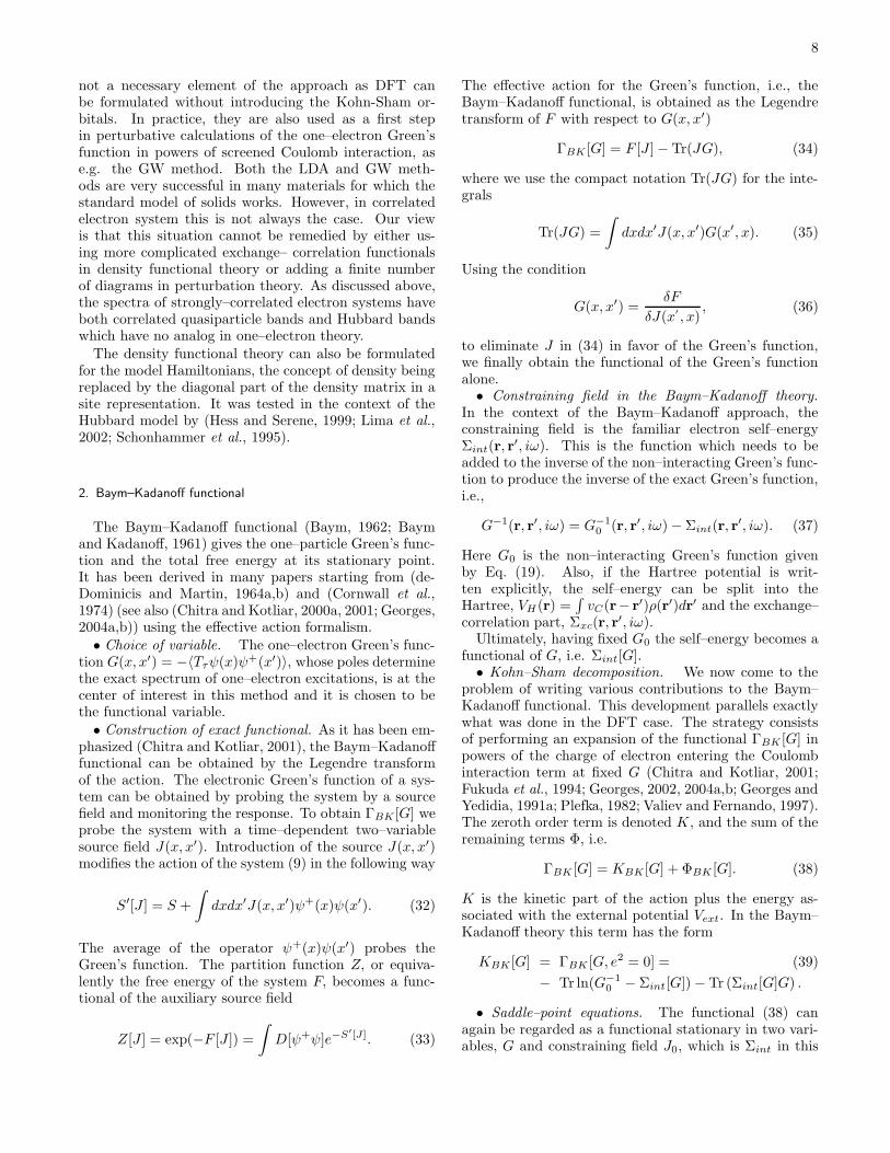
The functional formulation in terms of a “screened”interaction W allows one to formulate numerous ap-proximations to the many–body problem. The sim-plest approximation consists in keeping the lowest or-der Hartree–Fock graph in the functional ΨBK [G,W ].This is the celebrated GW approximation (Hedin, 1965;Hedin and Lundquist, 1969) (see Fig. 4). To treat strongcorrelations one has to introduce dynamical mean fieldideas, which amount to a restriction of the functionalsΦBK ,ΨBK to the local part of the Greens function (seesection II). It is also natural to restrict the correlationfunction of the Bose field W , which corresponds to in-cluding information about the four point function of the

Fermion field in the self-consistency condition, and goesunder the name of the Extended Dynamical Mean–FieldTheory (EDMFT) (Bray and Moore, 1980; Chitra andKotliar, 2001; Kajueter, 1996a; Kajueter and Kotliar,1996a; Sachdev and Ye, 1993; Sengupta and Georges,1995; Si and Smith, 1996; Smith and Si, 2000).

This methodology has been useful in incorporating ef-fects of the long range Coulomb interactions (Chitra andKotliar, 2000b) as well as in the study of heavy fermionquantum critical points, (Si et. al. et al., 1999; Si et al.,2001) and quantum spin glasses (Bray and Moore, 1980;Sachdev and Ye, 1993; Sengupta and Georges, 1995)

More explicitly, in order to zero the off–diagonalGreen’s functions (see Eq. (54)) we introduce a set oflocalized orbitals ΦRα(r) and express G and W throughan expansion in those orbitals.

G(r, r′, iω) =∑

RR′αβ

GRα,R′β(iω)Φ∗Rα(r)ΦR′β(r′), (52)

W (r, r′, iω) =∑

R1α,R2β,R3γ,R4δ

WR1α,R2β,R3γ,R4δ(iω)×

Φ∗R1α(r)Φ∗

R2β(r′)ΦR3γ(r′)ΦR4δ(r). (53)

The approximate EDMFT functional is obtained byrestriction of the correlation part of the Baym–Kadanofffunctional ΨBK to the diagonal parts of the G and Wmatrices:

ΨEDMFT = ΨBK [GRR,WRRRR] (54)

The EDMFT graphs are shown in Fig. 4.It is straightforward to combine the GW and EDMFT

approximations by keeping the nonlocal part of the ex-change graphs as well as the local parts of the correlationgraphs (see Fig. 4).

The GW approximation derived from the Baym–Kadanoff functional is a fully self–consistent approxi-mation which involves all electrons. In practice some-times two approximations are used: a) in pseudopotentialtreatments only the self–energy of the valence and con-duction electrons are considered and b) instead of eval-uating Π and Σ self–consistently with G and W , onedoes a “one–shot” or one iteration approximation whereΣ and Π are evaluated with G0, the bare Green’s func-tion which is sometimes taken as the LDA Kohn–ShamGreen’s function, i.e., Σ ≈ Σ[G0,W0] and Π = Π[G0].The validity of these approximations and importance ofthe self–consistency for the spectra evaluation was ex-plored in (Arnaud and Alouani, 2000; Holm, 1999; Holmand von Barth, 1998; Hybertsen and Louie, 1985; Tiagoet al., 2003; Wei Ku, 2002). The same issues arise in thecontext of GW+EDMFT (Sun and Kotliar, 2004).

At this point, the GW+EDMFT has been fully imple-mented on the one–band model Hamiltonian level (Sunand Kotliar, 2002, 2004). A combination of GW andLDA+DMFT was applied to Nickel, where W in the

11

ΦGW :wiji j

ΦEDMFT :wiii i + + ...

i i

ii

ΦGW+EDMFT:wiji j + + ...

i i

ii

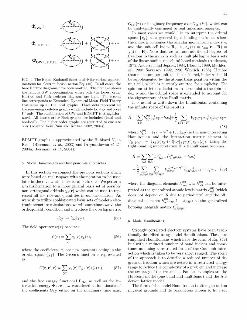
FIG. 4 The Baym–Kadanoff functional Φ for various approx-imations for electron–boson action Eq. (46). In all cases, thebare Hartree diagrams have been omitted. The first line showsthe famous GW approximation where only the lowest orderHartree and Fock skeleton diagrams are kept. The secondline corresponds to Extended–Dynamical Mean–Field Theorythat sums up all the local graphs. Three dots represent allthe remaining skeleton graphs which include local G and localW only. The combination of GW and EDMFT is straightfor-ward. All lowest order Fock graphs are included (local andnonlocal). The higher order graphs are restricted to one siteonly (adapted from (Sun and Kotliar, 2002, 2004)).

EDMFT graphs is approximated by the Hubbard U , inRefs. (Biermann et al., 2003) and (Aryasetiawan et al.,2004a; Biermann et al., 2004).

5. Model Hamiltonians and first principles approaches

In this section we connect the previous sections whichwere based on real r-space with the notation to be usedlater in the review which use local basis sets. We performa transformation to a more general basis set of possiblynon–orthogonal orbitals χξ(r) which can be used to rep-resent all the relevant quantities in our calculation. Aswe wish to utilize sophisticated basis sets of modern elec-tronic structure calculations, we will sometimes waive theorthogonality condition and introduce the overlap matrix

Oξξ′ = 〈χξ|χξ′〉. (55)

The field operator ψ(x) becomes

ψ(x) =∑

ξ

cξ(τ)χξ(r), (56)

where the coefficients cξ are new operators acting in theorbital space χξ. The Green’s function is representedas

G(r, r′, τ) =∑

ξξ′

χξ(r)Gξξ′ (τ)χ∗ξ′ (r′), (57)

and the free energy functional ΓBK as well as the in-teraction energy Φ are now considered as functionals ofthe coefficients Gξξ′ either on the imaginary time axis,

Gξξ′(τ) or imaginary frequency axis Gξξ′(iω), which canbe analytically continued to real times and energies.

In most cases we would like to interpret the orbitalspace χξ as a general tight–binding basis set wherethe index ξ combines the angular momentum index lm,and the unit cell index R, i.e., χξ(r) = χlm(r − R) =χα(r − R). Note that we can add additional degrees offreedom to the index α such as multiple kappa basis setsof the linear muffin–tin orbital based methods (Andersen,1975; Andersen and Jepsen, 1984; Bloechl, 1989; Methfes-sel, 1988; Savrasov, 1992, 1996; Weyrich, 1988). If morethan one atom per unit cell is considered, index α shouldbe supplemented by the atomic basis position within theunit cell, which is currently omitted for simplicity. Forspin unrestricted calculations α accumulates the spin in-dex σ and the orbital space is extended to account forthe eigenvectors of the Pauli matrix.

It is useful to write down the Hamiltonian containingthe infinite space of the orbitals

H =∑

ξξ′

h(0)ξξ′ [c

+ξ cξ′+h.c.]+

1

2

∑

ξξ′ξ′′ξ′′′

Vξξ′ξ′′ξ′′′c+ξ c+ξ′cξ′′cξ′′′ ,

(58)

where h(0)ξξ′ = 〈χξ|−∇2 +Vext|χξ′〉 is the non–interacting

Hamiltonian and the interaction matrix element isVξξ′ξ′′ξ′′′ = 〈χξ(r)χξ′ (r′)|vC |χξ′′(r′)χξ′′′(r)〉. Using thetight–binding interpretation this Hamiltonian becomes

H =∑

αβ

∑

RR′

h(0)αRβR′

(c+αRcβR′ + h.c.

)

+1

2

∑

αβγδ

∑

RR′R′′R′′′

V RR′R′′R′′′

αβγδ c+αRc+βR′cδR′′′cγR′′ , (59)

where the diagonal elements h(0)αRβR ≡ h

(0)αβ can be inter-

preted as the generalized atomic levels matrix ε(0)αβ (which

does not depend on R due to periodicity) and the off–

diagonal elements h(0)αRβR′(1 − δRR′) as the generalized

hopping integrals matrix t(0)αRβR′ .

6. Model Hamiltonians

Strongly correlated electron systems have been tradi-tionally described using model Hamiltonians. These aresimplified Hamiltonians which have the form of Eq. (59)but with a reduced number of band indices and some-times assuming a restricted form of the Coulomb inter-action which is taken to be very short ranged. The spiritof the approach is to describe a reduced number of de-grees of freedom which are active in a restricted energyrange to reduce the complexity of a problem and increasethe accuracy of the treatment. Famous examples are theHubbard model (one band and multiband) and the An-derson lattice model.

The form of the model Hamiltonian is often guessed onphysical grounds and its parameters chosen to fit a set

12

of experiments. In principle a more explicit constructioncan be carried out using tools such as screening canon-ical transformations first used by Bohm and Pines toeliminate the long range part of the Coulomb interaction(Bohm and Pines, 1951, 1952, 1953), or a Wilsonian par-tial elimination (or integrating out) of the high–energydegrees of freedom (Wilson, 1975). However, these pro-cedures are rarely used in practice.

One starts from an action describing a large numberof degrees of freedom (site and orbital omitted)

S[c+c] =

∫dx(c+O∂τ c+H [c+c]

), (60)

where the orbital overlap OαRβR′ appears and the Hamil-tonian could have the form (59). Second, one divides theset of operators in the path integral in cH describing the“high–energy” orbitals which one would like to eliminate,and cL describing the low–energy orbitals that one wouldlike to consider explicitly. The high–energy degrees offreedom are now integrated out. This operation definesthe effective action for the low–energy variables (Wilson,1983):

1

Zeffexp(−Seff [c+LcL]) =

1

Z

∫dc+HdcH exp(−S[c+Hc

+LcLcH ]).

(61)The transformation (61) generates retarded interactionsof arbitrarily high order. If we focus on sufficiently lowenergies, frequency dependence of the coupling constantsbeyond linear order and non–linearities beyond quarticorder can be neglected since they are irrelevant arounda Fermi liquid fixed point (Shankar, 1994). The result-ing physical problem can then be cast in the form of aneffective model Hamiltonian. Notice however that whenwe wish to consider a broad energy range the full fre-quency dependence of the couplings has to be kept asdemonstrated in an explicit approximate calculation us-ing the GW method (Aryasetiawan et al., 2004b). Thesame ideas can be implemented using canonical transfor-mations and examples of approximate implementation ofthis program are provided by the method of cell perturba-tion theory (Raimondi et al., 1996) and the generalizedtight-binding method (Ovchinnikov and Sandalov, 1989).

The concepts and the rational underlying the modelHamiltonian approach are rigorous. There are very fewstudies of the form of the Hamiltonians obtained byscreening and elimination of high–energy degrees of free-dom, and the values of the parameters present in thoseHamiltonians. Notice however that if a form for themodel Hamiltonian is postulated, any technique whichcan be used to treat Hamiltonians approximately, can bealso used to perform the elimination (61). A consider-able amount of effort has been devoted to the evalua-tions of the screened Coulomb parameter U for a givenmaterial. Note that this value is necessarily connectedto the basis set representation which is used in derivingthe model Hamiltonian. It should be thought as an effec-tively downfolded Hamiltonian to take into account the

fact that only the interactions at a given energy inter-val are included in the description of the system. Moregenerally, one needs to talk about frequency–dependentinteraction W which appears for example in the GWmethod. The outlined questions have been addressed inmany previous works (Dederichs et al., 1984; Hybertsenet al., 1989; Kotani, 2000; McMahan et al., 1988; Springerand Aryasetiawan, 1998). Probably, one of the most pop-ular methods here is a constrained density functionalapproach formulated with general projection operators(Dederichs et al., 1984; Meider and Springborg, 1998).First, one defines the orbitals set which will be used todefine correlated electrons. Second, the on–site densitymatrix defined for these orbitals is constrained by intro-ducing additional constraining fields in the density func-tional. Evaluating second order derivative of the totalenergy with respect to the density matrix should in prin-ciple give us the access to Us. The problem is how onesubtracts the kinetic energy part which appears in thisformulation of the problem. Gunnarsson (Gunnarsson,1990) and others (Freeman et al., 1987; McMahan andMartin, 1988; Norman and Freeman, 1986) have intro-duced a method which effectively cuts the hybridizationof matrix elements between correlated and uncorrelatedorbitals eliminating the kinetic contribution. This ap-proach was used by McMahan et al. (McMahan et al.,1988) in evaluating the Coulomb interaction parametersin the high–temperature superconductors. An alterna-tive method has been used by Hybertsen et al. (Hybert-sen et al., 1989) who performed simultaneous simulationsusing the LDA and solution of the model Hamiltonian atthe mean–field level. The total energy under the con-straint of fixed occupancies was evaluated within bothapproaches. The value of U is adjusted to make the twocalculations coincide.

Much work has been done by the group of Anisimovwho have performed evaluations of the Coulomb andexchange interactions for various systems such as NiO,MnO, CaCuO2 and so on (Anisimov et al., 1991). In-terestingly, the values of U deduced for such itinerantsystem as Fe can be as large as 6 eV (Anisimov and Gun-narsson, 1991). This highlights an important problem ondeciding which electrons participate in the screening pro-cess. As a rule of thumb, one can argue that if we con-sider the entire d-shell as a correlated set, and allow itsscreening by s- and p-electrons, the values of U appear tobe between 5 and 10 eV on average. On the other hand,in many situations crystal field splitting between t2g andeg levels allows us to talk about a subset of a given crys-tal field symmetry (say, t2g), and allowing screening byanother subset (say by eg). This usually leads to muchsmaller values of U within range of 1-4 eV.

It is possible to extract the value of U from GW cal-culations. The simplest way to define the parameterU = W (ω = 0). There are also attempts to avoidthe double counting inherent in that procedure (Aryase-tiawan et al., 2004b; Kotani, 2000; Springer and Aryase-tiawan, 1998; Zein, 2005; Zein and Antropov, 2002). The

13

values of U for Ni deduced in this way appeared to be2.2-3.3 eV which are quite reasonable. At the same timea strong energy dependence of the interaction has beenpointed out which also addresses an important problemof treating the full frequency–dependent interaction wheninformation in a broad energy range is required.

The process of eliminating degrees of freedom with theapproximations described above gives us a physically rig-orous way of thinking about effective Hamiltonians witheffective parameters which are screened by the degrees offreedom to be eliminated. Since we neglect retardationand terms above fourth order, the effective Hamiltonianwould have the same form as (59) where we only changethe meaning of the parameters. It should be regarded asthe effective Hamiltonian that one can use to treat therelevant degrees of freedom. If the dependence on theionic coordinates are kept, it can be used to obtain thetotal energy. If the interaction matrix turns out to beshort ranged or has a simple form, this effective Hamil-tonian could be identified with the Hubbard (Hubbard,1963) or with the Anderson (Anderson, 1961) Hamilto-nians.

Finally we comment on the meaning of an ab initioor a first–principles electronic structure calculation. Theterm implies that no empirically adjustable parametersare needed in order to predict physical properties of com-pounds, only the structure and the charges of atoms areused as an input. First–principles does not mean exact oraccurate or computationally inexpensive. If the effectiveHamiltonian is derived (i.e. if the functional integral orcanonical transformation needed to reduce the numberof degrees of freedom is performed by a well–defined pro-cedure which keeps track of the energy of the integratedout degrees of freedom as a function of the ionic coor-dinates) and the consequent Hamiltonian (59) is solvedsystematically, then we have a first–principles method.In practice, the derivation of the effective Hamiltonianor its solution may be inaccurate or impractical, and inthis case the ab initio method is not very useful. No-tice that Heff has the form of a “model Hamiltonian”and very often a dichotomy between model Hamiltoniansand first–principles calculations is made. What makes amodel calculation semi–empirical is the lack of a coherentderivation of the form of the “model Hamiltonian” andthe corresponding parameters.

II. SPECTRAL DENSITY FUNCTIONAL APPROACH

We see that a great variety of many–body techniquesdeveloped to attack real materials can be viewed from aunified perspective. The energetics and excitation spec-trum of the solid is deduced within different degrees ofapproximation from the stationary condition of a func-tional of an observable. The different approaches differin the choice of variable for the functional which is tobe extremized. Therefore, the choice of the variable is acentral issue since the exact form of the functional is un-

known and existing approximations entirely rely on thegiven variable.

In this review we present arguments that a “goodvariable” in the functional description of a strongly–correlated material is a “local” Green’s functionGloc(r, r

′, z). This is only a part of the exact electronicGreen’s function, but it can be presently computed withsome degree of accuracy. Thus we would like to formu-late a functional theory where the local spectral densityis the central quantity to be computed, i.e. to developa spectral density functional theory (SDFT). Note thatthe notion of locality by itself is arbitrary since we canprobe the Green’s function in a portion of a certain spacesuch as reciprocal space or real space. These are themost transparent forms where the local Green’s functioncan be defined. We can also probe the Green’s func-tion in a portion of the Hilbert space like Eq. (57) whenthe Green’s function is expanded in some basis set χξ.Here our interest can be associated, e.g, with diagonalelements of the matrix Gξξ′ .

As we see, locality is a basis set dependent property.Nevertheless, it is a very useful property because it maylead to a very economical description of the function.The choice of the appropriate Hilbert space is thereforecrucial if we would like to find an optimal description ofthe system with the accuracy proportional to the com-putational cost. Therefore we always rely on physical in-tuition when choosing a particular representation whichshould be tailored to a specific physical problem.

A. Functional of local Green’s function

We start from the Hamiltonian of the form (59). Onecan view it as the full Hamiltonian written in some com-plete tight–binding basis set. Alternatively one can re-gard the starting point (59) as a model Hamiltonian, asargued in the previous section, if an additional constantterm (which depends on the position of the atoms) is keptand (59) is carefully derived. This can represent the fullHamiltonian in the relevant energy range provided thatone neglects higher order interaction terms.

• Choice of variable and construction of the exact func-tional. The effective action construction of SDFT paral-lels that given in Introduction. The quantity of interest isthe local (on–site) part of the one–particle Green’s func-tion. It is generated by adding a local source Jloc,αβ(τ, τ ′)to the action

S′ = S+∑

Rαβ

∫Jloc,Rαβ(τ, τ ′)c+Rα(τ)cRβ(τ ′)dτdτ ′. (62)

The partition function Z, or equivalently the free energyof the system F , according to (33) becomes a functionalof the auxiliary source field and the local Green’s function

14

is given by the variational derivative

δF

δJloc,Rβα(τ ′, τ)= −

⟨TτcRα(τ)c+Rβ(τ ′)

⟩= Gloc,αβ(τ, τ ′).

(63)From Eq. (63) one expresses Jloc as a functional of Gloc

to obtain the effective action by the standard procedure

ΓSDFT [Gloc] = F [Jloc] − Tr (JlocGloc) . (64)

The extremum of this functional gives rise to the exactlocal spectral function Gloc and the total free energy F .

Below, we will introduce the Kohn–Sham representa-tion of the spectral density functional ΓSDFT similar towhat was done in the Baym–Kadanoff and density func-tional theories. A dynamical mean–field approximationto the functional will be introduced in order to deal withits interaction counterpart. The theory can be devel-oped along two alternative paths depending on whetherwe stress that it is a truncation of the exact functionalwhen expanding ΓSDFT in powers of the hopping (atomicexpansion) or in powers of the interaction (expansionaround the band limit). The latter case is the usualsituation encountered in DFT and the Baym–Kadanofftheory, while the former has only been applied to SDFTthus far.

1. A non–interacting reference system: bands in afrequency–dependent potential

• The constraining field in the context of SDFT. Inthe context of SDFT, the constraining field is definedas Mint,αβ(iω). This is the function that one needs toadd to the free Hamiltonian in order to obtain a desiredspectral function:

Gloc,αβ(iω) =∑

k

((iω+µ)I−h(0)(k)−Mint[Gloc](iω)

)−1

αβ

,

(65)

where I is a unit matrix, h(0)(k) is the Fourier trans-form (with respect to R − R′) of the bare one–electron

Hamiltonian h(0)αRβR′ entering (59). The assumption that

the equation (65) can be solved to define Mint,αβ(iω)as a function of Gloc,αβ(iω), is the SDFT version of theKohn–Sham representability condition of DFT. For DFTthis has been proved to exist under certain conditions,(for discussion of this problem see (Gross et al., 1996)).The SDFT condition has not been yet investigated indetail, but it seems to be a plausible assumption.• Significance of the constraining field in SDFT. If

the exact self–energy of the problem is momentum inde-pendent, then Mint,αβ(iω) coincides with the interactionpart of the self–energy. This statement resembles the ob-servation in DFT: if the self–energy of a system is mo-mentum and frequency independent then the self–energycoincides with the Kohn–Sham potential.

•Analog of the Kohn–Sham Green’s function. Hav-ing defined Mint,αβ(iω), we can introduce an auxiliaryGreen’s function GαRβR′(iω) connected to our new “in-teracting Kohn–Sham” particles. It is defined in the en-tire space by the relationship:

G−1αRβR′ (iω) ≡ G−1

0,αRβR′ (iω) − δRR′Mint,αβ(iω), (66)

where G−10 = (iω + µ)I − h(0)(k) (in Fourier space).

Mint,αβ(iω) was defined so that GαRβR′(iω) coincideswith the on–site Green’s function on a single site andthe Kohn–Sham Green’s function has the property

Gloc,αβ(iω) = δRR′GαRβR′(iω). (67)

Notice that Mint is a functional of Gloc and thereforeG is also a function of Gloc. If this relation can be in-verted, the functionals that where previously regarded asfunctionals of Gloc can be also regarded as functionals ofthe Kohn–Sham Green’s function G.• Exact Kohn–Sham decomposition. We separate the

functional ΓSDFT [Gloc] into the non–interacting con-tribution (this is the zeroth order term in an expan-sion in the Coulomb interactions), KSDFT [Gloc], andthe remaining interaction contribution, ΦSDFT [Gloc]:ΓSDFT [G] = KSDFT [Gloc]+ΦSDFT [Gloc]. With the helpof Mint or equivalently the Kohn–Sham Green’s functionG the non–interacting term in the spectral density func-tional theory can be represented (compare with (23) and(39)) as follows

KSDFT [Gloc] = −Tr ln(G−10 − δRR′Mint[Gloc])−

Tr (δRR′Mint[Gloc]Gloc) . (68)

Since G is a functional of Gloc, one can also view theentire spectral density functional ΓSDFT as a functionalof G:

ΓSDFT [G] = −Tr ln(G−10 − δRR′Mint[G])−

Tr (Mint[G]G) + ΦSDFT [Gloc[G]], (69)

where the unknown interaction part of the free energyΦSDFT [Gloc] is a functional of Gloc and

δGloc,αβ

δGαRβR′

= δRR′ , (70)

according to Eq. (67).• Exact representation of ΦSDFT . Spectral den-

sity functional theory requires the interaction functionalΦSDFT [Gloc]. Its explicit form is unavailable. How-ever we can express it via an introduction of an integralover the coupling constant λe2 multiplying the two–bodyinteraction term similar to the density functional the-ory (Gunnarsson and Lundqvist, 1976; Harris and Jones,1974) result. Considering ΓSDFT [Gloc, λ] at any interac-tion λ (which enters vC(r − r′)) we write

ΓSDFT [Gloc, e2] = ΓSDFT [Gloc, 0]+

∫ 1

0

dλ∂ΓSDFT [Gloc, λ]

∂λ.

(71)

15

Here the first term is simply the non–interacting partKSDFT [Gloc] as given by (68) which does not depend onλ. The second part is thus the unknown functional (seeEq. (7))

ΦSDFT [Gloc] =

∫ 1

0

dλ∂ΓSDFT [Gloc, λ]

∂λ(72)

=1

2

∫ 1

0

dλ∑

RR′R′′R′′′

∑

αβγδ

V RR′R′′R′′′

αβγδ 〈c+αRc+βR′cγR′′cδR′′′ 〉λ.

One can also further separate ΦSDFT [Gloc] intoEH [Gloc] + Φxc

SDFT [Gloc], where the Hartree term is afunctional of the density only.• Exact functional as a function of two variables.

The SDFT can also be viewed as a functional of twoindependent variables (Kotliar and Savrasov, 2001).This is equivalent to what is known as Harris–Foulkes–Methfessel functional within DFT (Foulkes, 1989; Harris,1985; Methfessel, 1995)

ΓSDFT [Gloc,Mint] = −∑

k

Tr ln[(iω + µ)I − h(0)(k) −Mint(iω)] − Tr (MintGloc) + ΦSDFT [Gloc]. (73)

Eq. (65) is a saddle point of the functional (73) definingMint = Mint[Gloc] and should be back–substituted toobtain ΓSDFT [Gloc].• Saddle point equations and their significance. Dif-

ferentiating the functional (73), one obtains a functionalequation for Gloc

Mint[Gloc] =δΦSDFT [Gloc]

δGloc. (74)

Combined with the definition of the constraining field(65) it gives the standard form of the DMFT equations.Note that thus far these are exact equations and the con-straining field Mint(iω) is by definition “local”, i.e. mo-mentum independent.

2. An interacting reference system: a dressed atom

We can obtain the spectral density functional byadopting a different reference system, namely the atom.The starting point of this approach is the Hamilto-nian (59) split into two parts (Chitra and Kotliar,2000a; Georges, 2004a,b): H = H0 + H1, where H0 =∑

RHat[R] with Hat defined as

Hat[R] =∑

αβ

h(0)αRβR[c+αRcβR + h.c.] (75)

+1

2

∑

αβγδ

V RRRRαβγδ c+αRc

+βRcδRcγR.

H1 is the interaction term used in the inversion methoddone in powers of λH1 (λ is a new coupling constant tobe set to unity at the end of the calculation).•The constraining field in SDFT. After an unper-

turbed Hamiltonian is chosen the constraining field is de-fined as the zeroth order term of the source in an expan-sion in the coupling constant. When the reference frameis the dressed atom, the constraining field turns out tobe the hybridization function of an Anderson impuritymodel (AIM) ∆[Gloc]αβ(τ, τ ′) (Anderson, 1961), which

plays a central role in the dynamical mean–field theory.It is defined as the (time dependent) field which mustbe added to Hat in order to generate the local Green’sfunction Gloc,αβ(τ, τ ′)

δFat

δ∆βα(τ ′, τ)= −

⟨Tτcα(τ)c+β (τ ′)

⟩∆

= Gloc,αβ(τ, τ ′),

(76)where

Fat[∆] = (77)

− ln

∫dc+dce−Sat[c

+c]−P

αβ

R∆αβ(τ,τ ′)c+

α (τ)cβ(τ ′)dτdτ ′

,

and the atomic action is given by

Sat[∆] =

∫dτ∑

αβ

c+α (τ)

(∂

∂τ− µ

)cβ(τ) +

∫dτHat(τ).

(78)Eq. (77) actually corresponds to an impurity problem

and Fat[∆] can be obtained by solving an Anderson im-purity model.•Kohn–Sham decomposition and its significance. The

Kohn–Sham decomposition separates the effective actioninto two parts: the zeroth order part of the effective ac-tion in the coupling constant Γ0[Gloc] ≡ ΓSDFT [Gloc, λ =0] and the rest (“exchange correlation part”). The func-tional corresponding to (73) is given by

ΓSDFT [Gloc, λ = 0] = Fat[∆[Gloc]] − Tr (∆[Gloc]Gloc) =

Tr lnGloc − Tr(G−1

at Gloc

)+ Φat[Gloc], (79)

with the G−1at,αβ(iω) = (iω + µ)δαβ − h

(0)αβ . Fat is the

free energy when λ = 0 and Φat is the sum of all two–particle irreducible diagrams constructed with the localvertex V RRRR

αβγδ and Gloc.• Saddle point equations and their significance. The

saddle point equations determine the exact spectral func-tion (and the exact Weiss field). They have the form

−⟨Tτcα(τ)c+β (τ ′)

⟩∆

= Gloc,αβ(τ, τ ′), (80)

16

∆αβ(τ, τ ′) =δ∆Γ

δGloc,βα(τ ′, τ), (81)

where ∆Γ can be expressed using coupling constant in-tegration as is in Eq. (5) (Georges, 2004a,b). This set ofequations describes an atom or a set of atoms in the unitcell embedded in the medium. ∆ is the exact Weiss field(with respect to the expansion around the atomic limit)which is defined from the equation for the local Green’sfunction Gloc (see Eq. (76)). The general Weiss source∆ in this case should be identified with the hybridizationof the Anderson impurity model.

When the system is adequately represented as a col-lection of paramagnetic atoms, the Weiss field is a weakperturbation representing the environment to which it isweakly coupled. Since this is an exact construction, itcan also describe the band limit when the hybridizationbecomes large.

3. Construction of approximations: dynamical mean–fieldtheory as an approximation.

The SDFT should be viewed as a separate exact the-ory whose manifestly local constraining field is an aux-iliary mass operator introduced to reproduce the localpart of the Green’s function of the system, exactly likethe Kohn–Sham potential is an auxiliary operator intro-duced to reproduce the density of the electrons in DFT.However, to obtain practical results, we need practicalapproximations. The dynamical mean–field theory canbe thought of as an approximation to the exact SDFTfunctional in the same spirit as LDA appears as an ap-proximation to the exact DFT functional.

The diagrammatic rules for the exact SDFT functionalcan be developed but they are more complicated than inthe Baym–Kadanoff theory as discussed in (Chitra andKotliar, 2000a). The single–site DMFT approximationto this functional consists of taking ΦSDFT [Gloc] to be asum of all graphs (on a single site R), constructed withV RRRR

αβγδ as a vertex and Gloc as a propagator, which

are two–particle irreducible, namely ΦDMFT [Gloc] =Φat[Gloc]. This together with Eq. (73) defines the DMFTapproximation to the exact spectral density functional.

It is possible to arrive at this functional by summingup diagrams (Chitra and Kotliar, 2000a) or using thecoupling constant integration trick (Georges, 2004a,b)(see Eq. (7)) with a coupling dependent Greens functionhaving the DMFT form, namely with a local self-energy.This results in

ΓDMFT (Gloc ii) =∑

i

Fat[∆(Gloc ii)] (82)

−∑

k

Tr ln((iω + µ)I − h(0)(k) −Mint(Gloc ii)

)

+Tr ln(−Mint(Gloc ii) + iω + µ− h(0) − ∆(iω)

).

with Mint(Gloc ii) in Eq. (82) the self-energy of the An-derson impurity model. It is useful to have a formu-

lation of this DMFT functional as a function of threevariables, (Kotliar and Savrasov, 2001) namely combin-ing the hybridization with that atomic Greens functionto form the Weiss function G−1

0 = G−1at − ∆, one can ob-

tain the DMFT equations from the stationary point of afunctional of Gloc, Mint and the Weiss field G0:

Γ[Gloc,Mint,G0] = Fimp[G−10 ] − Tr ln[Gloc] − (83)

Tr ln(iω + µ− h0[k] −Mint) +

Tr[(G0−1 −Mint −G−1

loc)Gloc].

One can eliminate Gloc and Mint from (83) usingthe stationary conditions and recover a functional of theWeiss field function only. This form of the functional,applied to the Hubbard model, allowed the analyticaldetermination of the nature of the transition and thecharacterization of the zero temperature critical points(Kotliar, 1999a). Alternatively eliminating G0 and Gloc

in favor of Mint one obtains the DMFT approximationto the self-energy functional discussed in section I.B.2.

4. Cavity construction

An alternative view to derive the DMFT approxima-tion is by means of the cavity construction. This ap-proach gives complementary insights to the nature of theDMFT and its extensions. It is remarkable that the sum-mation over all local diagrams can be performed exactlyvia introduction of an auxiliary quantum impurity modelsubjected to a self–consistency condition (Georges andKotliar, 1992; Georges et al., 1996). If this impurity isconsidered as a cluster C, either a dynamical cluster ap-proximation or cellular DMFT technique can be used.In single–site DMFT, considering the effective action Sin Eq. (60), the integration volume is separated into theimpurity Vimp and the remaining volume is referred toas the bath: V − Vimp = Vbath. The action is now rep-resented as the action of the cluster cell, Vimp plus theaction of the bath, Vbath, plus the interaction betweenthose two. We are interested in the local effective actionSimp of the cluster degrees of freedom only, which is ob-tained conceptually by integrating out the bath in thefunctional integral

1

Zimpexp[−Simp] =

1

Z

∫

Vbath

D[c†c] exp[−S], (84)

where Zimp and Z are the corresponding partition func-tions. Carrying out this integration and neglecting allquartic and higher order terms (which is correct in theinfinite dimension limit) we arrive to the result (Georgesand Kotliar, 1992)

Simp = −∑

αβ

∫dτdτ ′c+α (τ)G−1

0,αβ(τ, τ ′)cβ(τ ′) (85)

+1

2

∑

αβγδ

∫dτdτ ′c+α (τ)c+β (τ ′)Vαβγδ(τ, τ

′)cγ(τ ′)cδ(τ).

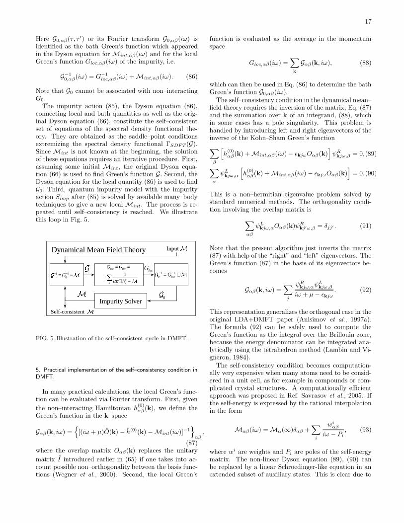
17

Here G0,αβ(τ, τ ′) or its Fourier transform G0,αβ(iω) isidentified as the bath Green’s function which appearedin the Dyson equation for Mint,αβ(iω) and for the localGreen’s function Gloc,αβ(iω) of the impurity, i.e.

G−10,αβ(iω) = G−1

loc,αβ(iω) + Mint,αβ(iω). (86)

Note that G0 cannot be associated with non–interactingG0.

The impurity action (85), the Dyson equation (86),connecting local and bath quantities as well as the orig-inal Dyson equation (66), constitute the self–consistentset of equations of the spectral density functional the-ory. They are obtained as the saddle–point conditionsextremizing the spectral density functional ΓSDFT (G).Since Mint is not known at the beginning, the solutionof these equations requires an iterative procedure. First,assuming some initial Mint, the original Dyson equa-tion (66) is used to find Green’s function G. Second, theDyson equation for the local quantity (86) is used to findG0. Third, quantum impurity model with the impurityaction Simp after (85) is solved by available many–bodytechniques to give a new local Mint. The process is re-peated until self–consistency is reached. We illustratethis loop in Fig. 5.

1 10G− −= −

1 10 locG− −= +

0

1loc RR

k k

G

i hω

= =

+ −

locG

0

Impurity Solver

Input

Self-consistent

Dynamical Mean Field Theory

FIG. 5 Illustration of the self–consistent cycle in DMFT.

5. Practical implementation of the self–consistency condition inDMFT.

In many practical calculations, the local Green’s func-tion can be evaluated via Fourier transform. First, given

the non–interacting Hamiltonian h(0)αβ(k), we define the

Green’s function in the k–space

Gαβ(k, iω) =[(iω + µ)O(k) − h(0)(k) −Mint(iω)]−1

αβ,

(87)where the overlap matrix Oαβ(k) replaces the unitary

matrix I introduced earlier in (65) if one takes into ac-count possible non–orthogonality between the basis func-tions (Wegner et al., 2000). Second, the local Green’s

function is evaluated as the average in the momentumspace

Gloc,αβ(iω) =∑

k

Gαβ(k, iω), (88)

which can then be used in Eq. (86) to determine the bathGreen’s function G0,αβ(iω).

The self–consistency condition in the dynamical mean–field theory requires the inversion of the matrix, Eq. (87)and the summation over k of an integrand, (88), whichin some cases has a pole singularity. This problem ishandled by introducing left and right eigenvectors of theinverse of the Kohn–Sham Green’s function

∑

β

[h

(0)αβ(k) + Mint,αβ(iω) − εkjωOαβ(k)

]ψR

kjω,β = 0,(89)

∑

α

ψLkjω,α

[h

(0)αβ(k) + Mint,αβ(iω) − εkjωOαβ(k)

]= 0.(90)

This is a non–hermitian eigenvalue problem solved bystandard numerical methods. The orthogonality condi-tion involving the overlap matrix is

∑

αβ

ψLkjω,αOαβ(k)ψR

kj′ω,β = δjj′ . (91)

Note that the present algorithm just inverts the matrix(87) with help of the “right” and “left” eigenvectors. TheGreen’s function (87) in the basis of its eigenvectors be-comes

Gαβ(k, iω) =∑

j

ψRkjω,αψ

Lkjω,β

iω + µ− εkjω. (92)

This representation generalizes the orthogonal case in theoriginal LDA+DMFT paper (Anisimov et al., 1997a).The formula (92) can be safely used to compute theGreen’s function as the integral over the Brillouin zone,because the energy denominator can be integrated ana-lytically using the tetrahedron method (Lambin and Vi-gneron, 1984).

The self-consistency condition becomes computation-ally very expensive when many atoms need to be consid-ered in a unit cell, as for example in compounds or com-plicated crystal structures. A computationally efficientapproach was proposed in Ref. Savrasov et al., 2005. Ifthe self-energy is expressed by the rational interpolationin the form

Mαβ(iω) = Mα(∞)δαβ +∑

i

wiαβ

iω − Pi, (93)

where wi are weights and Pi are poles of the self-energymatrix. The non-linear Dyson equation (89), (90) canbe replaced by a linear Schroedinger-like equation in anextended subset of auxiliary states. This is clear due to

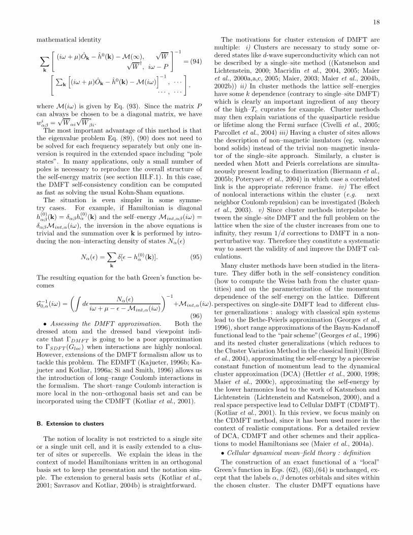
18

mathematical identity

∑

k

[(iω + µ)Ok − h0(k) −M(∞),

√W√

W†, iω − P

]−1

= (94)

[ ∑k

[(iω + µ)Ok − h0(k) −M(iω)

]−1

, · · ·· · · , · · ·

].

where M(iω) is given by Eq. (93). Since the matrix Pcan always be chosen to be a diagonal matrix, we have

wiαβ =

√Wαi

√W

∗

βi.The most important advantage of this method is that

the eigenvalue problem Eq. (89), (90) does not need tobe solved for each frequency separately but only one in-version is required in the extended space including “polestates”. In many applications, only a small number ofpoles is necessary to reproduce the overall structure ofthe self-energy matrix (see section III.F.1). In this case,the DMFT self-consistency condition can be computedas fast as solving the usual Kohn-Sham equations.

The situation is even simpler in some symme-try cases. For example, if Hamiltonian is diagonal

h(0)αβ(k) = δαβh

(0)α (k) and the self–energy Mint,αβ(iω) =

δαβMint,α(iω), the inversion in the above equations istrivial and the summation over k is performed by intro-ducing the non–interacting density of states Nα(ε)

Nα(ε) =∑

k

δ[ε− h(0)α (k)]. (95)

The resulting equation for the bath Green’s function be-comes

G−10,α(iω) =

(∫dε

Nα(ε)

iω + µ− ε−Mint,α(iω)

)−1

+Mint,α(iω).

(96)• Assessing the DMFT approximation. Both the

dressed atom and the dressed band viewpoint indi-cate that ΓDMFT is going to be a poor approximationto ΓSDFT (Gloc) when interactions are highly nonlocal.However, extensions of the DMFT formalism allow us totackle this problem. The EDMFT (Kajueter, 1996b; Ka-jueter and Kotliar, 1996a; Si and Smith, 1996) allows usthe introduction of long–range Coulomb interactions inthe formalism. The short–range Coulomb interaction ismore local in the non–orthogonal basis set and can beincorporated using the CDMFT (Kotliar et al., 2001).

B. Extension to clusters

The notion of locality is not restricted to a single siteor a single unit cell, and it is easily extended to a clus-ter of sites or supercells. We explain the ideas in thecontext of model Hamiltonians written in an orthogonalbasis set to keep the presentation and the notation sim-ple. The extension to general basis sets (Kotliar et al.,2001; Savrasov and Kotliar, 2004b) is straightforward.

The motivations for cluster extension of DMFT aremultiple: i) Clusters are necessary to study some or-dered states like d-wave superconductivity which can notbe described by a single–site method ((Katsnelson andLichtenstein, 2000; Macridin et al., 2004, 2005; Maieret al., 2000a,a,c, 2005; Maier, 2003; Maier et al., 2004b,2002b)) ii) In cluster methods the lattice self–energieshave some k dependence (contrary to single–site DMFT)which is clearly an important ingredient of any theoryof the high–Tc cuprates for example. Cluster methodsmay then explain variations of the quasiparticle residueor lifetime along the Fermi surface (Civelli et al., 2005;Parcollet et al., 2004) iii) Having a cluster of sites allowsthe description of non–magnetic insulators (eg. valencebond solids) instead of the trivial non–magnetic insula-tor of the single–site approach. Similarly, a cluster isneeded when Mott and Peierls correlations are simulta-neously present leading to dimerization (Biermann et al.,2005b; Poteryaev et al., 2004) in which case a correlatedlink is the appropriate reference frame. iv) The effectof nonlocal interactions within the cluster (e.g. nextneighbor Coulomb repulsion) can be investigated (Bolechet al., 2003). v) Since cluster methods interpolate be-tween the single–site DMFT and the full problem on thelattice when the size of the cluster increases from one toinfinity, they resum 1/d corrections to DMFT in a non-perturbative way. Therefore they constitute a systematicway to assert the validity of and improve the DMFT cal-culations.

Many cluster methods have been studied in the litera-ture. They differ both in the self–consistency condition(how to compute the Weiss bath from the cluster quan-tities) and on the parameterization of the momentumdependence of the self–energy on the lattice. Differentperspectives on single-site DMFT lead to different clus-ter generalizations : analogy with classical spin systemslead to the Bethe-Peierls approximation (Georges et al.,1996), short range approximations of the Baym-Kadanofffunctional lead to the “pair scheme”(Georges et al., 1996)and its nested cluster generalizations (which reduces tothe Cluster Variation Method in the classical limit)(Biroliet al., 2004), approximating the self-energy by a piecewiseconstant function of momentum lead to the dynamicalcluster approximation (DCA) (Hettler et al., 2000, 1998;Maier et al., 2000c), approximating the self-energy bythe lower harmonics lead to the work of Katsnelson andLichtenstein (Lichtenstein and Katsnelson, 2000), and areal space perspective lead to Cellular DMFT (CDMFT).(Kotliar et al., 2001). In this review, we focus mainly onthe CDMFT method, since it has been used more in thecontext of realistic computations. For a detailed reviewof DCA, CDMFT and other schemes and their applica-tions to model Hamiltonians see (Maier et al., 2004a).

• Cellular dynamical mean–field theory : definition

The construction of an exact functional of a “local”Green’s function in Eqs. (62), (63),(64) is unchanged, ex-cept that the labels α, β denotes orbitals and sites withinthe chosen cluster. The cluster DMFT equations have

19

the form (65), (86), where h0[k] is now replaced by t(K)the matrix of hoppings in supercell notation and we usethe notation ΣC(iωn) for the cluster self–energy (notethat the notation Mint was used for this quantity in thepreceding sections).

G−10 (iωn) =

(∑

K∈RBZ

(iωn + µ− t(K) − ΣC(iωn)

)−1)−1

+ ΣC(iωn), (97)

where the sum overK is taken over the Reduced BrillouinZone (RBZ) of the superlattice and normalized.

Just like single–site DMFT, one can either viewCDMFT as an approximation to an exact functional tocompute the cluster Green’s function, or as an approxi-mation to the exact Baym–Kadanoff functional obtainedby restricting it to the Green’s functions on the sites re-stricted to a cluster and its translation by a supercelllattice vector (see Eq. (102) below) (Georges, 2002;Maier and Jarrell, 2002). From a spectral density func-tional point of view, Eqs. (66), (67), and the equationMint[G] = δΦSDFT /δGloc can be viewed as the exactequations provided that the exact functional ΦSDFT isknown.

A good approximation to the “exact functional”,whose knowledge would deliver us the exact clusterGreen’s function, is obtained by restricting the exactBaym–Kadanoff functional. In this case, it is restrictedto a cluster and all its translations by a supercell vec-tor. Denoting by C the set of couples (i, j) where i andj belong to the same cluster (see Fig. 6 for an example),

ΦSDFTCDMFT = ΦBK |Gij=0 if (i,j)/∈C (98)

Alternatively the CDMFT equations can be derivedfrom the point of view of a functional of the Weiss fieldgeneralizing Eq. (82) from single sites to supercells asshown in Fig. 6. A fundamental concept in DMFT isthat of a Weiss field. This is the function describing theenvironment that one needs to add to an interacting butlocal problem to obtain the correct local Greens functionof an extended system. Now expressed in terms of theWeiss field of the cluster G−1

0 = G−1at − ∆. This concept

can be used to highlight the connection of the mean fieldtheory of lattice systems with impurity models and therelation of their free energies (Georges et al., 1996). Forthis purpose it is useful to define the DMFT functionalof three variables, (Kotliar and Savrasov, 2001) Gloc, Σand the Weiss field G0:

ΓCDMFT [G,Σ,G0] = ΣcellsFcell[G−10 ] − Tr ln[G] (99)

−Tr ln[G](iω + µ− t[k] − Σ

)+ Tr[(G0

−1 − Σ −G−1)G]

Extremizing this functional gives again the standardCDMFT equations.• CDMFT : approximation of lattice quantities

FIG. 6 Example of a 2× 2 superlattice construction to defineCDMFT on a plaquette. Notice that the definition is depen-dent on the tiling of space by supercells and is therefore notunique

The impurity model delivers cluster quantities. Inorder to make a connection with the original latticeproblem, we need to formulate estimates for the latticeGreen’s function. A natural way to produce these esti-mates is by considering the superlattice (SL) (see Fig. 6)and constructing lattice objects from superlattice objectsby averaging the relevant quantities to restore periodic-ity, namely

Wlatt(i− j) ≈ 1

Ns

∑

k

WSLk,k+i−j , (100)

where Ns represents the total number of sites, and i, j, kare site indices. Notice that Eq. (100) represents a super-lattice average, not a cluster average. In particular, ifW is the cluster irreducible cumulant, Mc ≡ G−1

c + ∆(where ∆ is the hybridization) or the cluster self-energyΣ all the contributions with k and k + i − j belong-ing to different cells are zero by construction. The lat-tice Greens function can then be reconstructed from thelattice cumulant (Stanescu, 2005) or the lattice self-energy (Biroli and Kotliar, 2002; Kotliar et al., 2001).Namely Glatt(k, ω) ≈ (ω − t(k) + µ − Σlatt(k, ω))−1 or

Glatt(k, ω) ≈ (−t(k) + Mlatt(k, ω)−1

)−1 . Criteria formore general periodizations respecting causality were de-rived in ref (Biroli and Kotliar, 2002). Another alter-native suggested originally by Senechal and Tremblayis to directly periodize the Green’s function, i.e. applyEq. (100) with W = G to obtain (Senechal et al., 2000)

G(k, ω) =1

Nc

∑

a,b∈C

[M−1c − tk]−1

ab eik(ra−rb), (101)

where tk is the Fourier transform of the “hopping” on thesuper-lattice, and Nc the number of sites in the cluster.

For example, consider the two-dimensional Hubbardmodel on a square lattice within a four-site approxima-tion (plaquette) in which square symmetry is preserved.After performing the average (100) and then taking the

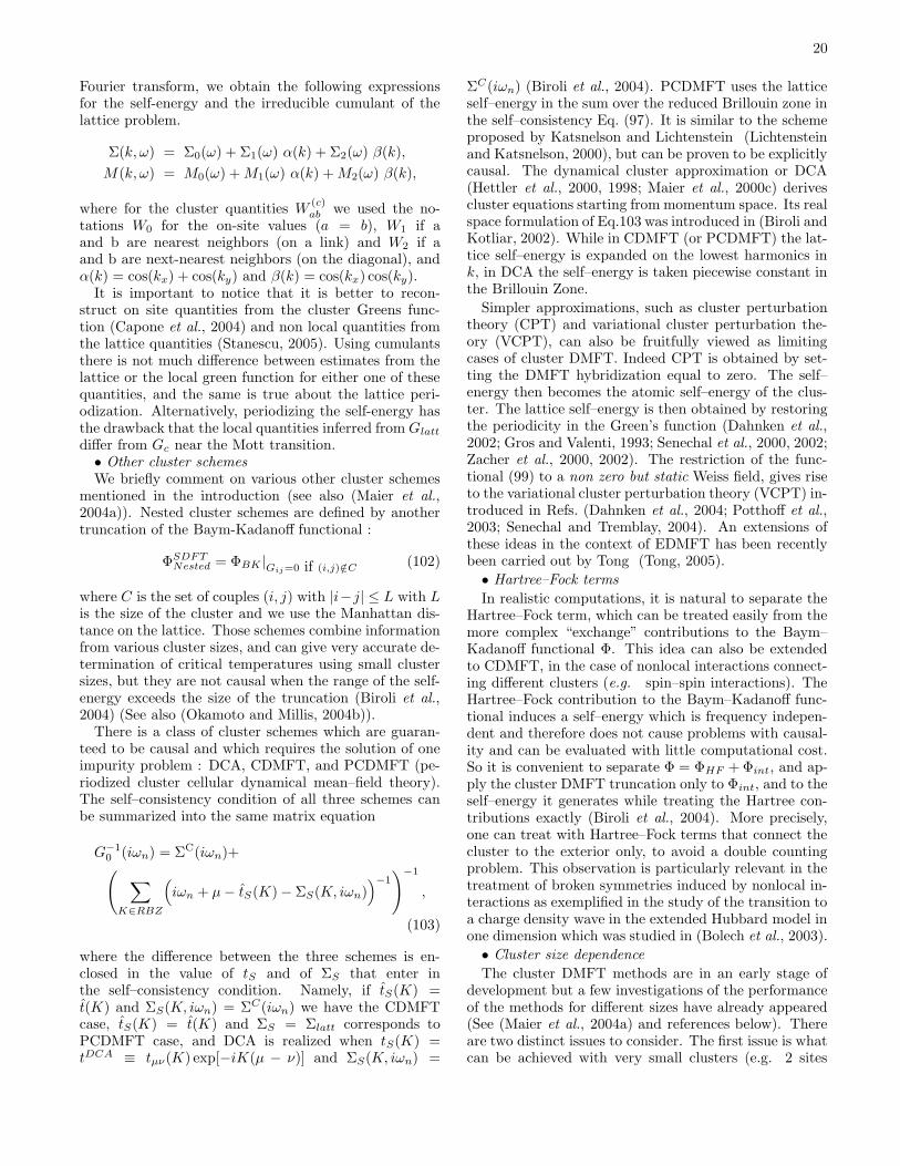
20

Fourier transform, we obtain the following expressionsfor the self-energy and the irreducible cumulant of thelattice problem.

Σ(k, ω) = Σ0(ω) + Σ1(ω) α(k) + Σ2(ω) β(k),

M(k, ω) = M0(ω) +M1(ω) α(k) +M2(ω) β(k),

where for the cluster quantities W(c)ab we used the no-

tations W0 for the on-site values (a = b), W1 if aand b are nearest neighbors (on a link) and W2 if aand b are next-nearest neighbors (on the diagonal), andα(k) = cos(kx) + cos(ky) and β(k) = cos(kx) cos(ky).

It is important to notice that it is better to recon-struct on site quantities from the cluster Greens func-tion (Capone et al., 2004) and non local quantities fromthe lattice quantities (Stanescu, 2005). Using cumulantsthere is not much difference between estimates from thelattice or the local green function for either one of thesequantities, and the same is true about the lattice peri-odization. Alternatively, periodizing the self-energy hasthe drawback that the local quantities inferred from Glatt

differ from Gc near the Mott transition.• Other cluster schemesWe briefly comment on various other cluster schemes

mentioned in the introduction (see also (Maier et al.,2004a)). Nested cluster schemes are defined by anothertruncation of the Baym-Kadanoff functional :

ΦSDFTNested = ΦBK |Gij=0 if (i,j)/∈C (102)

where C is the set of couples (i, j) with |i−j| ≤ L with Lis the size of the cluster and we use the Manhattan dis-tance on the lattice. Those schemes combine informationfrom various cluster sizes, and can give very accurate de-termination of critical temperatures using small clustersizes, but they are not causal when the range of the self-energy exceeds the size of the truncation (Biroli et al.,2004) (See also (Okamoto and Millis, 2004b)).

There is a class of cluster schemes which are guaran-teed to be causal and which requires the solution of oneimpurity problem : DCA, CDMFT, and PCDMFT (pe-riodized cluster cellular dynamical mean–field theory).The self–consistency condition of all three schemes canbe summarized into the same matrix equation

G−10 (iωn) = ΣC(iωn)+(

∑

K∈RBZ

(iωn + µ− tS(K) − ΣS(K, iωn)

)−1)−1

,

(103)

where the difference between the three schemes is en-closed in the value of tS and of ΣS that enter inthe self–consistency condition. Namely, if tS(K) =t(K) and ΣS(K, iωn) = ΣC(iωn) we have the CDMFTcase, tS(K) = t(K) and ΣS = Σlatt corresponds toPCDMFT case, and DCA is realized when tS(K) =tDCA ≡ tµν(K) exp[−iK(µ − ν)] and ΣS(K, iωn) =

ΣC(iωn) (Biroli et al., 2004). PCDMFT uses the latticeself–energy in the sum over the reduced Brillouin zone inthe self–consistency Eq. (97). It is similar to the schemeproposed by Katsnelson and Lichtenstein (Lichtensteinand Katsnelson, 2000), but can be proven to be explicitlycausal. The dynamical cluster approximation or DCA(Hettler et al., 2000, 1998; Maier et al., 2000c) derivescluster equations starting from momentum space. Its realspace formulation of Eq.103 was introduced in (Biroli andKotliar, 2002). While in CDMFT (or PCDMFT) the lat-tice self–energy is expanded on the lowest harmonics ink, in DCA the self–energy is taken piecewise constant inthe Brillouin Zone.

Simpler approximations, such as cluster perturbationtheory (CPT) and variational cluster perturbation the-ory (VCPT), can also be fruitfully viewed as limitingcases of cluster DMFT. Indeed CPT is obtained by set-ting the DMFT hybridization equal to zero. The self–energy then becomes the atomic self–energy of the clus-ter. The lattice self–energy is then obtained by restoringthe periodicity in the Green’s function (Dahnken et al.,2002; Gros and Valenti, 1993; Senechal et al., 2000, 2002;Zacher et al., 2000, 2002). The restriction of the func-tional (99) to a non zero but static Weiss field, gives riseto the variational cluster perturbation theory (VCPT) in-troduced in Refs. (Dahnken et al., 2004; Potthoff et al.,2003; Senechal and Tremblay, 2004). An extensions ofthese ideas in the context of EDMFT has been recentlybeen carried out by Tong (Tong, 2005).

• Hartree–Fock terms

In realistic computations, it is natural to separate theHartree–Fock term, which can be treated easily from themore complex “exchange” contributions to the Baym–Kadanoff functional Φ. This idea can also be extendedto CDMFT, in the case of nonlocal interactions connect-ing different clusters (e.g. spin–spin interactions). TheHartree–Fock contribution to the Baym–Kadanoff func-tional induces a self–energy which is frequency indepen-dent and therefore does not cause problems with causal-ity and can be evaluated with little computational cost.So it is convenient to separate Φ = ΦHF + Φint, and ap-ply the cluster DMFT truncation only to Φint, and to theself–energy it generates while treating the Hartree con-tributions exactly (Biroli et al., 2004). More precisely,one can treat with Hartree–Fock terms that connect thecluster to the exterior only, to avoid a double countingproblem. This observation is particularly relevant in thetreatment of broken symmetries induced by nonlocal in-teractions as exemplified in the study of the transition toa charge density wave in the extended Hubbard model inone dimension which was studied in (Bolech et al., 2003).

• Cluster size dependence

The cluster DMFT methods are in an early stage ofdevelopment but a few investigations of the performanceof the methods for different sizes have already appeared(See (Maier et al., 2004a) and references below). Thereare two distinct issues to consider. The first issue is whatcan be achieved with very small clusters (e.g. 2 sites

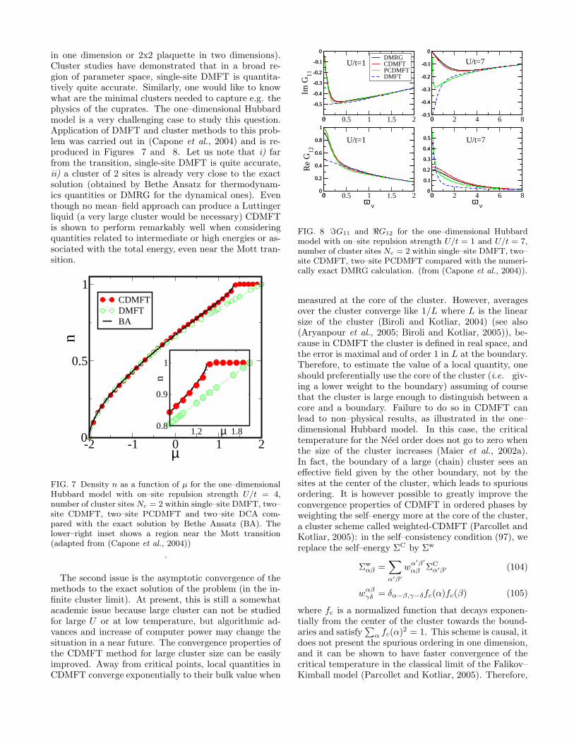
21

in one dimension or 2x2 plaquette in two dimensions).Cluster studies have demonstrated that in a broad re-gion of parameter space, single-site DMFT is quantita-tively quite accurate. Similarly, one would like to knowwhat are the minimal clusters needed to capture e.g. thephysics of the cuprates. The one–dimensional Hubbardmodel is a very challenging case to study this question.Application of DMFT and cluster methods to this prob-lem was carried out in (Capone et al., 2004) and is re-produced in Figures 7 and 8. Let us note that i) farfrom the transition, single-site DMFT is quite accurate,ii) a cluster of 2 sites is already very close to the exactsolution (obtained by Bethe Ansatz for thermodynam-ics quantities or DMRG for the dynamical ones). Eventhough no mean–field approach can produce a Luttingerliquid (a very large cluster would be necessary) CDMFTis shown to perform remarkably well when consideringquantities related to intermediate or high energies or as-sociated with the total energy, even near the Mott tran-sition.

-2 -1 0 1 2µ

0

0.5

1

n

CDMFTDMFTBA

1.2 1.8µ0.8

0.9

1

n

FIG. 7 Density n as a function of µ for the one–dimensionalHubbard model with on–site repulsion strength U/t = 4,number of cluster sites Nc = 2 within single–site DMFT, two–site CDMFT, two–site PCDMFT and two–site DCA com-pared with the exact solution by Bethe Ansatz (BA). Thelower–right inset shows a region near the Mott transition(adapted from (Capone et al., 2004))

.

The second issue is the asymptotic convergence of themethods to the exact solution of the problem (in the in-finite cluster limit). At present, this is still a somewhatacademic issue because large cluster can not be studiedfor large U or at low temperature, but algorithmic ad-vances and increase of computer power may change thesituation in a near future. The convergence properties ofthe CDMFT method for large cluster size can be easilyimproved. Away from critical points, local quantities inCDMFT converge exponentially to their bulk value when

0 0.5 1 1.5 2

-0.5

-0.4

-0.3

-0.2

-0.1

0

Im G

11

0

-0.5

-0.4

-0.3

-0.2

-0.1

0DMRGCDMFTPCDMFTDMFT

0 2 4 6 8-0.5

-0.4

-0.3

-0.2

-0.1

0

0-0.5

-0.4

-0.3

-0.2

-0.1

0

0 0.5 1 1.5 2ω ν

0

0.2

0.4

0.6

0.8

1

Re

G12

00

0.2

0.4

0.6

0.8

1

0 2 4 6 8ω ν

0

0.1

0.2

0.3

0.4

0.5

00

0.1

0.2

0.3

0.4

0.5

U/t=1 U/t=7

U/t=7U/t=1

FIG. 8 =G11 and <G12 for the one–dimensional Hubbardmodel with on–site repulsion strength U/t = 1 and U/t = 7,number of cluster sites Nc = 2 within single–site DMFT, two–site CDMFT, two–site PCDMFT compared with the numeri-cally exact DMRG calculation. (from (Capone et al., 2004)).

measured at the core of the cluster. However, averagesover the cluster converge like 1/L where L is the linearsize of the cluster (Biroli and Kotliar, 2004) (see also(Aryanpour et al., 2005; Biroli and Kotliar, 2005)), be-cause in CDMFT the cluster is defined in real space, andthe error is maximal and of order 1 in L at the boundary.Therefore, to estimate the value of a local quantity, oneshould preferentially use the core of the cluster (i.e. giv-ing a lower weight to the boundary) assuming of coursethat the cluster is large enough to distinguish between acore and a boundary. Failure to do so in CDMFT canlead to non–physical results, as illustrated in the one–dimensional Hubbard model. In this case, the criticaltemperature for the Neel order does not go to zero whenthe size of the cluster increases (Maier et al., 2002a).In fact, the boundary of a large (chain) cluster sees aneffective field given by the other boundary, not by thesites at the center of the cluster, which leads to spuriousordering. It is however possible to greatly improve theconvergence properties of CDMFT in ordered phases byweighting the self–energy more at the core of the cluster,a cluster scheme called weighted-CDMFT (Parcollet andKotliar, 2005): in the self–consistency condition (97), wereplace the self–energy ΣC by Σw

Σwαβ =

∑

α′β′

wα′β′

αβ ΣCα′β′ (104)

wαβγδ = δα−β,γ−δfc(α)fc(β) (105)

where fc is a normalized function that decays exponen-tially from the center of the cluster towards the bound-aries and satisfy

∑α fc(α)2 = 1. This scheme is causal, it

does not present the spurious ordering in one dimension,and it can be shown to have faster convergence of thecritical temperature in the classical limit of the Falikov–Kimball model (Parcollet and Kotliar, 2005). Therefore,

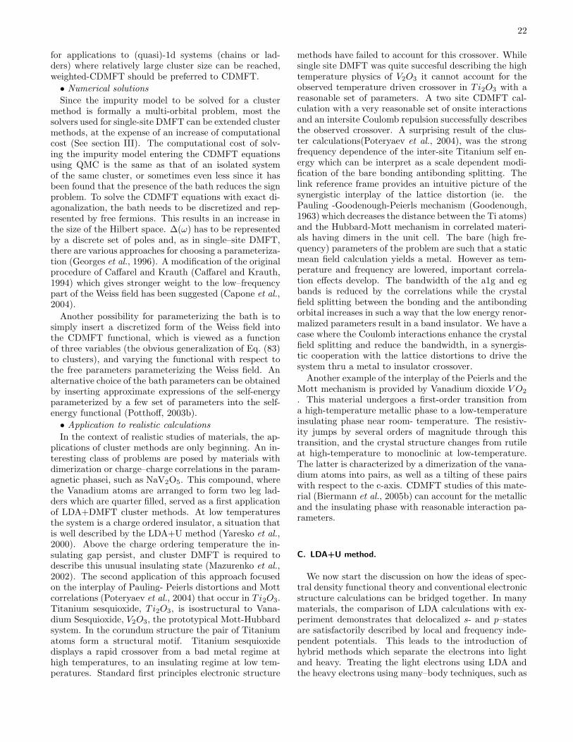
22

for applications to (quasi)-1d systems (chains or lad-ders) where relatively large cluster size can be reached,weighted-CDMFT should be preferred to CDMFT.

• Numerical solutions

Since the impurity model to be solved for a clustermethod is formally a multi-orbital problem, most thesolvers used for single-site DMFT can be extended clustermethods, at the expense of an increase of computationalcost (See section III). The computational cost of solv-ing the impurity model entering the CDMFT equationsusing QMC is the same as that of an isolated systemof the same cluster, or sometimes even less since it hasbeen found that the presence of the bath reduces the signproblem. To solve the CDMFT equations with exact di-agonalization, the bath needs to be discretized and rep-resented by free fermions. This results in an increase inthe size of the Hilbert space. ∆(ω) has to be representedby a discrete set of poles and, as in single–site DMFT,there are various approaches for choosing a parameteriza-tion (Georges et al., 1996). A modification of the originalprocedure of Caffarel and Krauth (Caffarel and Krauth,1994) which gives stronger weight to the low–frequencypart of the Weiss field has been suggested (Capone et al.,2004).

Another possibility for parameterizing the bath is tosimply insert a discretized form of the Weiss field intothe CDMFT functional, which is viewed as a functionof three variables (the obvious generalization of Eq. (83)to clusters), and varying the functional with respect tothe free parameters parameterizing the Weiss field. Analternative choice of the bath parameters can be obtainedby inserting approximate expressions of the self-energyparameterized by a few set of parameters into the self-energy functional (Potthoff, 2003b).

• Application to realistic calculations

In the context of realistic studies of materials, the ap-plications of cluster methods are only beginning. An in-teresting class of problems are posed by materials withdimerization or charge–charge correlations in the param-agnetic phasei, such as NaV2O5. This compound, wherethe Vanadium atoms are arranged to form two leg lad-ders which are quarter filled, served as a first applicationof LDA+DMFT cluster methods. At low temperaturesthe system is a charge ordered insulator, a situation thatis well described by the LDA+U method (Yaresko et al.,2000). Above the charge ordering temperature the in-sulating gap persist, and cluster DMFT is required todescribe this unusual insulating state (Mazurenko et al.,2002). The second application of this approach focusedon the interplay of Pauling- Peierls distortions and Mottcorrelations (Poteryaev et al., 2004) that occur in T i2O3.Titanium sesquioxide, T i2O3, is isostructural to Vana-dium Sesquioxide, V2O3, the prototypical Mott-Hubbardsystem. In the corundum structure the pair of Titaniumatoms form a structural motif. Titanium sesquioxidedisplays a rapid crossover from a bad metal regime athigh temperatures, to an insulating regime at low tem-peratures. Standard first principles electronic structure

methods have failed to account for this crossover. Whilesingle site DMFT was quite succesful describing the hightemperature physics of V2O3 it cannot account for theobserved temperature driven crossover in T i2O3 with areasonable set of parameters. A two site CDMFT cal-culation with a very reasonable set of onsite interactionsand an intersite Coulomb repulsion successfully describesthe observed crossover. A surprising result of the clus-ter calculations(Poteryaev et al., 2004), was the strongfrequency dependence of the inter-site Titanium self en-ergy which can be interpret as a scale dependent modi-fication of the bare bonding antibonding splitting. Thelink reference frame provides an intuitive picture of thesynergistic interplay of the lattice distortion (ie. thePauling -Goodenough-Peierls mechanism (Goodenough,1963) which decreases the distance between the Ti atoms)and the Hubbard-Mott mechanism in correlated materi-als having dimers in the unit cell. The bare (high fre-quency) parameters of the problem are such that a staticmean field calculation yields a metal. However as tem-perature and frequency are lowered, important correla-tion effects develop. The bandwidth of the a1g and egbands is reduced by the correlations while the crystalfield splitting between the bonding and the antibondingorbital increases in such a way that the low energy renor-malized parameters result in a band insulator. We have acase where the Coulomb interactions enhance the crystalfield splitting and reduce the bandwidth, in a synergis-tic cooperation with the lattice distortions to drive thesystem thru a metal to insulator crossover.

Another example of the interplay of the Peierls and theMott mechanism is provided by Vanadium dioxide V O2

. This material undergoes a first-order transition froma high-temperature metallic phase to a low-temperatureinsulating phase near room- temperature. The resistiv-ity jumps by several orders of magnitude through thistransition, and the crystal structure changes from rutileat high-temperature to monoclinic at low-temperature.The latter is characterized by a dimerization of the vana-dium atoms into pairs, as well as a tilting of these pairswith respect to the c-axis. CDMFT studies of this mate-rial (Biermann et al., 2005b) can account for the metallicand the insulating phase with reasonable interaction pa-rameters.

C. LDA+U method.

We now start the discussion on how the ideas of spec-tral density functional theory and conventional electronicstructure calculations can be bridged together. In manymaterials, the comparison of LDA calculations with ex-periment demonstrates that delocalized s- and p–statesare satisfactorily described by local and frequency inde-pendent potentials. This leads to the introduction ofhybrid methods which separate the electrons into lightand heavy. Treating the light electrons using LDA andthe heavy electrons using many–body techniques, such as

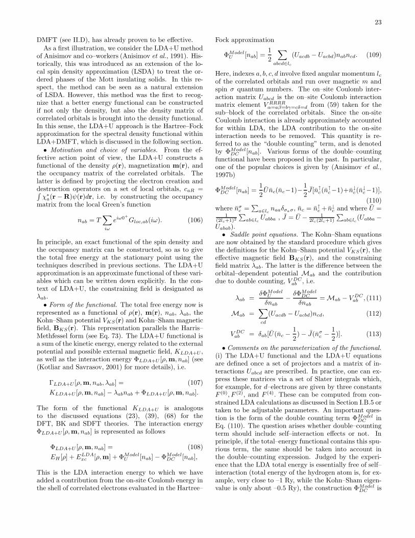
23

DMFT (see II.D), has already proven to be effective.As a first illustration, we consider the LDA+U method

of Anisimov and co–workers (Anisimov et al., 1991). His-torically, this was introduced as an extension of the lo-cal spin density approximation (LSDA) to treat the or-dered phases of the Mott insulating solids. In this re-spect, the method can be seen as a natural extensionof LSDA. However, this method was the first to recog-nize that a better energy functional can be constructedif not only the density, but also the density matrix ofcorrelated orbitals is brought into the density functional.In this sense, the LDA+U approach is the Hartree–Fockapproximation for the spectral density functional withinLDA+DMFT, which is discussed in the following section.• Motivation and choice of variables. From the ef-

fective action point of view, the LDA+U constructs afunctional of the density ρ(r), magnetization m(r), andthe occupancy matrix of the correlated orbitals. Thelatter is defined by projecting the electron creation anddestruction operators on a set of local orbitals, caR =∫χ∗

a(r −R)ψ(r)dr, i.e. by constructing the occupancymatrix from the local Green’s function

nab = T∑

iω

eiω0+

Gloc,ab(iω). (106)

In principle, an exact functional of the spin density andthe occupancy matrix can be constructed, so as to givethe total free energy at the stationary point using thetechniques described in previous sections. The LDA+Uapproximation is an approximate functional of these vari-ables which can be written down explicitly. In the con-text of LDA+U, the constraining field is designated asλab.• Form of the functional. The total free energy now is

represented as a functional of ρ(r), m(r), nab, λab, theKohn–Sham potential VKS(r) and Kohn–Sham magneticfield, BKS(r). This representation parallels the Harris–Methfessel form (see Eq. 73). The LDA+U functional isa sum of the kinetic energy, energy related to the externalpotential and possible external magnetic field, KLDA+U ,as well as the interaction energy ΦLDA+U [ρ,m, nab] (see(Kotliar and Savrasov, 2001) for more details), i.e.

ΓLDA+U [ρ,m, nab, λab] = (107)

KLDA+U [ρ,m, nab] − λabnab + ΦLDA+U [ρ,m, nab].

The form of the functional KLDA+U is analogousto the discussed equations (23), (39), (68) for theDFT, BK and SDFT theories. The interaction energyΦLDA+U [ρ,m, nab] is represented as follows

ΦLDA+U [ρ,m, nab] = (108)

EH [ρ] +ELDAxc [ρ,m] + ΦModel

U [nab] − ΦModelDC [nab],

This is the LDA interaction energy to which we haveadded a contribution from the on-site Coulomb energy inthe shell of correlated electrons evaluated in the Hartree–

Fock approximation

ΦModelU [nab] =

1

2

∑

abcd∈lc

(Uacdb − Uacbd)nabncd. (109)

Here, indexes a, b, c, d involve fixed angular momentum lcof the correlated orbitals and run over magnetic m andspin σ quantum numbers. The on–site Coulomb inter-action matrix Uabcd is the on–site Coulomb interactionmatrix element V RRRR

α=aβ=bγ=cδ=d from (59) taken for thesub–block of the correlated orbitals. Since the on-siteCoulomb interaction is already approximately accountedfor within LDA, the LDA contribution to the on-siteinteraction needs to be removed. This quantity is re-ferred to as the “double counting” term, and is denotedby ΦModel

DC [nab]. Various forms of the double–countingfunctional have been proposed in the past. In particular,one of the popular choices is given by (Anisimov et al.,1997b)

ΦModelDC [nab] =

1

2U nc(nc−1)− 1

2J [n↑

c(n↑c−1)+n↓

c(n↓c−1)],

(110)where nσ

c =∑

a∈lcnaaδσaσ , nc = n↑

c + n↓c and where U =

1(2lc+1)2

∑ab∈lc

Uabba , J = U − 12lc(2lc+1)

∑ab∈lc

(Uabba −Uabab).• Saddle point equations. The Kohn–Sham equations

are now obtained by the standard procedure which givesthe definitions for the Kohn–Sham potential VKS(r), theeffective magnetic field BKS(r), and the constrainingfield matrix λab. The latter is the difference between theorbital–dependent potential Mab and the contributiondue to double counting, V DC

ab , i.e.

λab =δΦModel

U

δnab− δΦModel

DC

δnab= Mab − V DC

ab , (111)

Mab =∑

cd

(Uacdb − Uacbd)ncd, (112)

V DCab = δab[U(nc −

1

2) − J(nσ

c − 1

2)]. (113)

• Comments on the parameterization of the functional.(i) The LDA+U functional and the LDA+U equationsare defined once a set of projectors and a matrix of in-teractions Uabcd are prescribed. In practice, one can ex-press these matrices via a set of Slater integrals which,for example, for d–electrons are given by three constantsF (0), F (2), and F (4). These can be computed from con-strained LDA calculations as discussed in Section I.B.5 ortaken to be adjustable parameters. An important ques-tion is the form of the double counting term ΦModel

DC inEq. (110). The question arises whether double–countingterm should include self–interaction effects or not. Inprinciple, if the total–energy functional contains this spu-rious term, the same should be taken into account inthe double–counting expression. Judged by the experi-ence that the LDA total energy is essentially free of self–interaction (total energy of the hydrogen atom is, for ex-ample, very close to –1 Ry, while the Kohn–Sham eigen-value is only about –0.5 Ry), the construction ΦModel

DC is

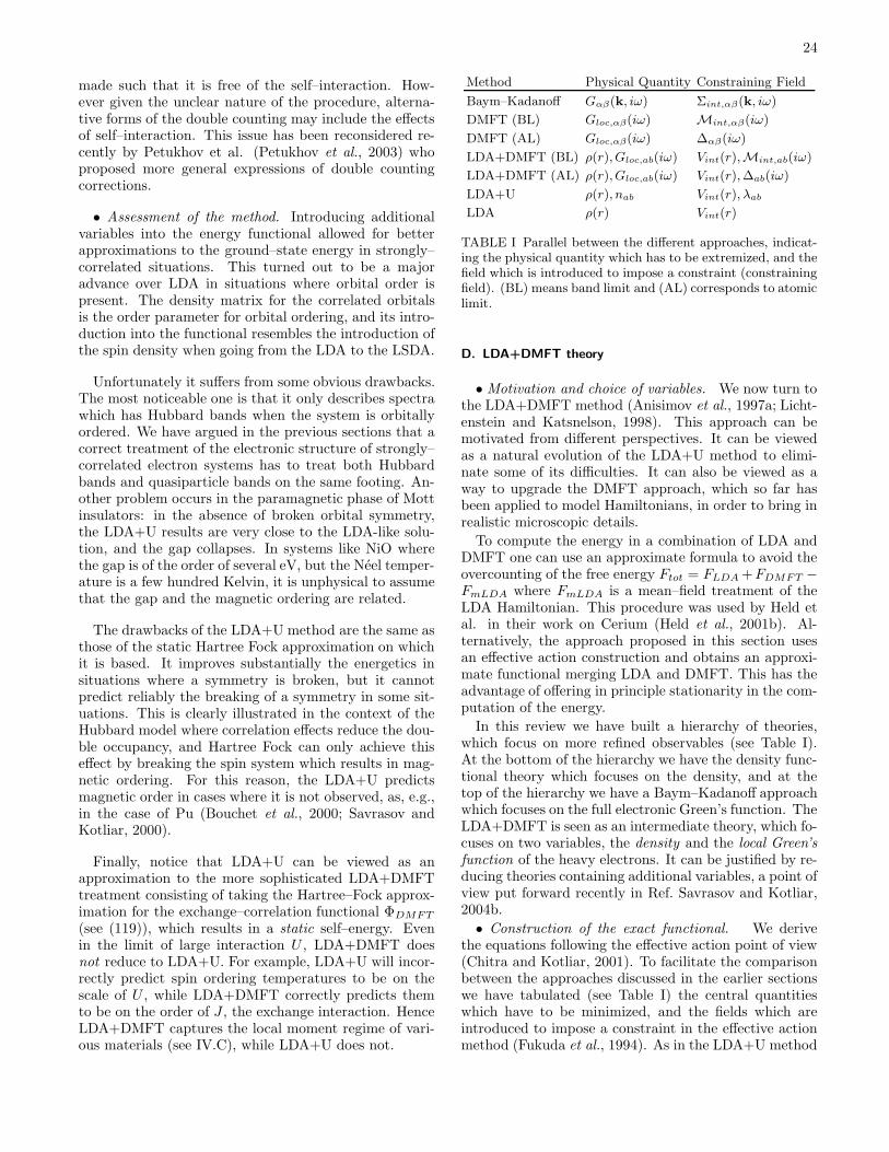
24

made such that it is free of the self–interaction. How-ever given the unclear nature of the procedure, alterna-tive forms of the double counting may include the effectsof self–interaction. This issue has been reconsidered re-cently by Petukhov et al. (Petukhov et al., 2003) whoproposed more general expressions of double countingcorrections.

• Assessment of the method. Introducing additionalvariables into the energy functional allowed for betterapproximations to the ground–state energy in strongly–correlated situations. This turned out to be a majoradvance over LDA in situations where orbital order ispresent. The density matrix for the correlated orbitalsis the order parameter for orbital ordering, and its intro-duction into the functional resembles the introduction ofthe spin density when going from the LDA to the LSDA.

Unfortunately it suffers from some obvious drawbacks.The most noticeable one is that it only describes spectrawhich has Hubbard bands when the system is orbitallyordered. We have argued in the previous sections that acorrect treatment of the electronic structure of strongly–correlated electron systems has to treat both Hubbardbands and quasiparticle bands on the same footing. An-other problem occurs in the paramagnetic phase of Mottinsulators: in the absence of broken orbital symmetry,the LDA+U results are very close to the LDA-like solu-tion, and the gap collapses. In systems like NiO wherethe gap is of the order of several eV, but the Neel temper-ature is a few hundred Kelvin, it is unphysical to assumethat the gap and the magnetic ordering are related.

The drawbacks of the LDA+U method are the same asthose of the static Hartree Fock approximation on whichit is based. It improves substantially the energetics insituations where a symmetry is broken, but it cannotpredict reliably the breaking of a symmetry in some sit-uations. This is clearly illustrated in the context of theHubbard model where correlation effects reduce the dou-ble occupancy, and Hartree Fock can only achieve thiseffect by breaking the spin system which results in mag-netic ordering. For this reason, the LDA+U predictsmagnetic order in cases where it is not observed, as, e.g.,in the case of Pu (Bouchet et al., 2000; Savrasov andKotliar, 2000).

Finally, notice that LDA+U can be viewed as anapproximation to the more sophisticated LDA+DMFTtreatment consisting of taking the Hartree–Fock approx-imation for the exchange–correlation functional ΦDMFT

(see (119)), which results in a static self–energy. Evenin the limit of large interaction U , LDA+DMFT doesnot reduce to LDA+U. For example, LDA+U will incor-rectly predict spin ordering temperatures to be on thescale of U , while LDA+DMFT correctly predicts themto be on the order of J , the exchange interaction. HenceLDA+DMFT captures the local moment regime of vari-ous materials (see IV.C), while LDA+U does not.

Method Physical Quantity Constraining Field

Baym–Kadanoff Gαβ(k, iω) Σint,αβ(k, iω)

DMFT (BL) Gloc,αβ(iω) Mint,αβ(iω)

DMFT (AL) Gloc,αβ(iω) ∆αβ(iω)

LDA+DMFT (BL) ρ(r),Gloc,ab(iω) Vint(r),Mint,ab(iω)

LDA+DMFT (AL) ρ(r),Gloc,ab(iω) Vint(r), ∆ab(iω)

LDA+U ρ(r), nab Vint(r), λab

LDA ρ(r) Vint(r)

TABLE I Parallel between the different approaches, indicat-ing the physical quantity which has to be extremized, and thefield which is introduced to impose a constraint (constrainingfield). (BL) means band limit and (AL) corresponds to atomiclimit.

D. LDA+DMFT theory

• Motivation and choice of variables. We now turn tothe LDA+DMFT method (Anisimov et al., 1997a; Licht-enstein and Katsnelson, 1998). This approach can bemotivated from different perspectives. It can be viewedas a natural evolution of the LDA+U method to elimi-nate some of its difficulties. It can also be viewed as away to upgrade the DMFT approach, which so far hasbeen applied to model Hamiltonians, in order to bring inrealistic microscopic details.

To compute the energy in a combination of LDA andDMFT one can use an approximate formula to avoid theovercounting of the free energy Ftot = FLDA +FDMFT −FmLDA where FmLDA is a mean–field treatment of theLDA Hamiltonian. This procedure was used by Held etal. in their work on Cerium (Held et al., 2001b). Al-ternatively, the approach proposed in this section usesan effective action construction and obtains an approxi-mate functional merging LDA and DMFT. This has theadvantage of offering in principle stationarity in the com-putation of the energy.

In this review we have built a hierarchy of theories,which focus on more refined observables (see Table I).At the bottom of the hierarchy we have the density func-tional theory which focuses on the density, and at thetop of the hierarchy we have a Baym–Kadanoff approachwhich focuses on the full electronic Green’s function. TheLDA+DMFT is seen as an intermediate theory, which fo-cuses on two variables, the density and the local Green’sfunction of the heavy electrons. It can be justified by re-ducing theories containing additional variables, a point ofview put forward recently in Ref. Savrasov and Kotliar,2004b.

• Construction of the exact functional. We derivethe equations following the effective action point of view(Chitra and Kotliar, 2001). To facilitate the comparisonbetween the approaches discussed in the earlier sectionswe have tabulated (see Table I) the central quantitieswhich have to be minimized, and the fields which areintroduced to impose a constraint in the effective actionmethod (Fukuda et al., 1994). As in the LDA+U method

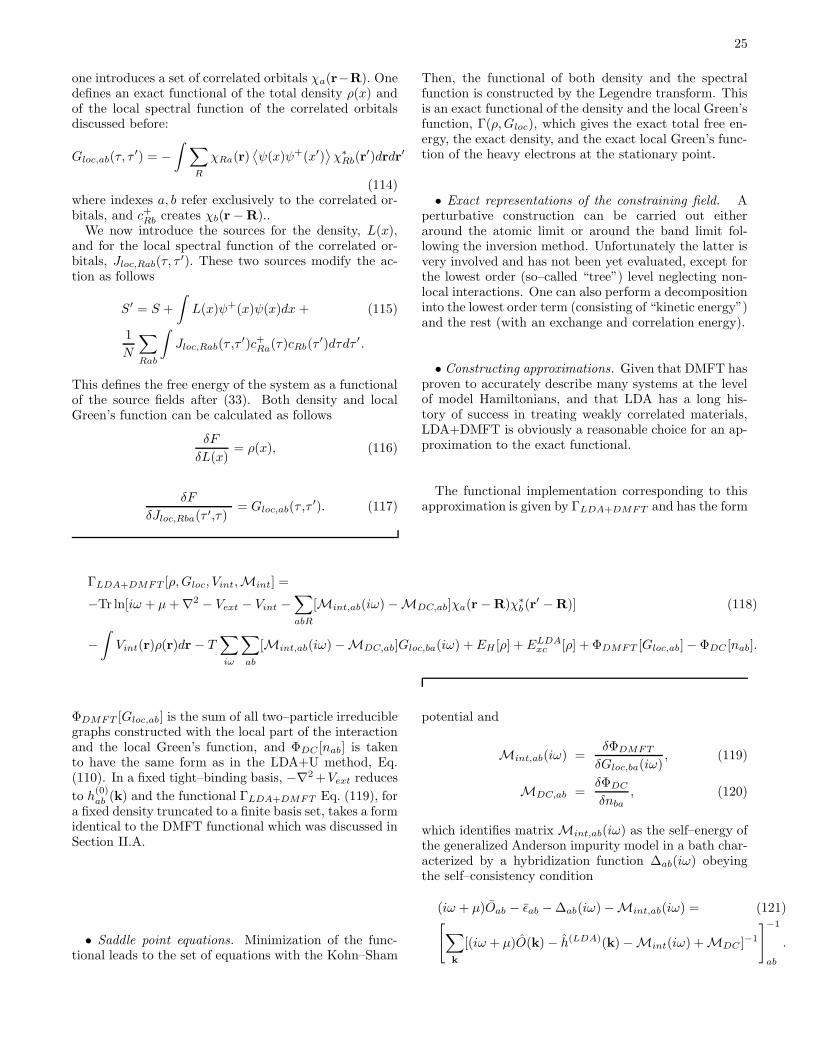
25

one introduces a set of correlated orbitals χa(r−R). Onedefines an exact functional of the total density ρ(x) andof the local spectral function of the correlated orbitalsdiscussed before:

Gloc,ab(τ, τ′) = −

∫ ∑

R

χRa(r)⟨ψ(x)ψ+(x′)

⟩χ∗

Rb(r′)drdr′

(114)where indexes a, b refer exclusively to the correlated or-bitals, and c+Rb creates χb(r −R)..

We now introduce the sources for the density, L(x),and for the local spectral function of the correlated or-bitals, Jloc,Rab(τ, τ

′). These two sources modify the ac-tion as follows

S′ = S +

∫L(x)ψ+(x)ψ(x)dx + (115)

1

N

∑

Rab

∫Jloc,Rab(τ ,τ

′)c+Ra(τ)cRb(τ′)dτdτ ′ .

This defines the free energy of the system as a functionalof the source fields after (33). Both density and localGreen’s function can be calculated as follows

δF

δL(x)= ρ(x), (116)

δF

δJloc,Rba(τ ′,τ)= Gloc,ab(τ ,τ

′). (117)

Then, the functional of both density and the spectralfunction is constructed by the Legendre transform. Thisis an exact functional of the density and the local Green’sfunction, Γ(ρ,Gloc), which gives the exact total free en-ergy, the exact density, and the exact local Green’s func-tion of the heavy electrons at the stationary point.

• Exact representations of the constraining field. Aperturbative construction can be carried out eitheraround the atomic limit or around the band limit fol-lowing the inversion method. Unfortunately the latter isvery involved and has not been yet evaluated, except forthe lowest order (so–called “tree”) level neglecting non-local interactions. One can also perform a decompositioninto the lowest order term (consisting of “kinetic energy”)and the rest (with an exchange and correlation energy).

• Constructing approximations. Given that DMFT hasproven to accurately describe many systems at the levelof model Hamiltonians, and that LDA has a long his-tory of success in treating weakly correlated materials,LDA+DMFT is obviously a reasonable choice for an ap-proximation to the exact functional.

The functional implementation corresponding to thisapproximation is given by ΓLDA+DMFT and has the form

ΓLDA+DMFT [ρ,Gloc, Vint,Mint] =

−Tr ln[iω + µ+ ∇2 − Vext − Vint −∑

abR

[Mint,ab(iω) −MDC,ab]χa(r −R)χ∗b (r

′ −R)] (118)

−∫Vint(r)ρ(r)dr − T

∑

iω

∑

ab

[Mint,ab(iω) −MDC,ab]Gloc,ba(iω) +EH [ρ] +ELDAxc [ρ] + ΦDMFT [Gloc,ab] − ΦDC [nab].

ΦDMFT [Gloc,ab] is the sum of all two–particle irreduciblegraphs constructed with the local part of the interactionand the local Green’s function, and ΦDC [nab] is takento have the same form as in the LDA+U method, Eq.(110). In a fixed tight–binding basis, −∇2 +Vext reduces

to h(0)ab (k) and the functional ΓLDA+DMFT Eq. (119), for

a fixed density truncated to a finite basis set, takes a formidentical to the DMFT functional which was discussed inSection II.A.

• Saddle point equations. Minimization of the func-tional leads to the set of equations with the Kohn–Sham

potential and

Mint,ab(iω) =δΦDMFT

δGloc,ba(iω), (119)

MDC,ab =δΦDC

δnba, (120)

which identifies matrix Mint,ab(iω) as the self–energy ofthe generalized Anderson impurity model in a bath char-acterized by a hybridization function ∆ab(iω) obeyingthe self–consistency condition

(iω + µ)Oab − εab − ∆ab(iω) −Mint,ab(iω) = (121)[∑

k

[(iω + µ)O(k) − h(LDA)(k) −Mint(iω) + MDC ]−1

]−1

ab

.

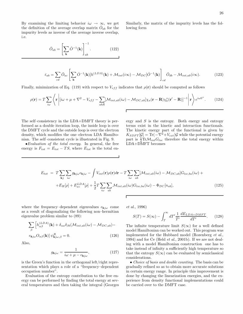
26

By examining the limiting behavior iω → ∞, we getthe definition of the average overlap matrix Oab for theimpurity levels as inverse of the average inverse overlap,i.e.

Oab =

[∑

k

O−1(k)

]−1

ab

. (122)

Similarly, the matrix of the impurity levels has the fol-lowing form

εab =∑

cd

Oac

[∑

k

O−1(k)[h(LDA)(k) + Mint(i∞) −MDC ]O−1(k)

]

cd

Odb −Mint,ab(i∞). (123)

Finally, minimization of Eq. (119) with respect to Veff indicates that ρ(r) should be computed as follows

ρ(r) = T∑

iω

⟨r

∣∣∣∣∣[iω + µ+ ∇2 − Veff −∑

abR

[Mint,ab(iω) −MDC,ab]χa(r −R)χ∗b (r

′ −R)]−1

∣∣∣∣∣ r⟩eiω0+

. (124)

The self–consistency in the LDA+DMFT theory is per-formed as a double iteration loop, the inside loop is overthe DMFT cycle and the outside loop is over the electrondensity, which modifies the one–electron LDA Hamilto-nian. The self–consistent cycle is illustrated in Fig. 9.•Evaluation of the total energy. In general, the free

energy is Ftot = Etot − TS, where Etot is the total en-

ergy and S is the entropy. Both energy and entropyterms exist in the kinetic and interaction functionals.The kinetic energy part of the functional is given byKSDFT [G] = Tr(−∇2+Vext)G while the potential energypart is 1

2TrMintGloc therefore the total energy withinLDA+DMFT becomes

Etot = T∑

kj

∑

iω

gkjωεkjω −∫Vint(r)ρ(r)dr − T

∑

iω

∑

ab

[Mint,ab(iω) −MDC,ab]Gloc,ba(iω) +

+EH [ρ] +ELDAxc [ρ] +

1

2T∑

iω

∑

ab

Mint,ab(iω)Gloc,ba(iω) − ΦDC [nab], (125)

where the frequency–dependent eigenvalues εkjω comeas a result of diagonalizing the following non–hermitianeigenvalue problem similar to (89):

∑

β

[h

(LDA)αβ (k) + δαaδβb(Mint,ab(iω) −MDC,ab)−

εkjωOαβ(k)]ψRkjω,β = 0. (126)

Also,

gkjω =1

iω + µ− εkjω, (127)

is the Green’s function in the orthogonal left/right repre-sentation which plays a role of a “frequency–dependentoccupation number”.

Evaluation of the entropy contribution to the free en-ergy can be performed by finding the total energy at sev-eral temperatures and then taking the integral (Georges

et al., 1996)

S(T ) = S(∞) −∫ ∞

T

dT ′ 1

T ′

dELDA+DMFT

dT ′. (128)

The infinite temperature limit S(∞) for a well definedmodel Hamiltonian can be worked out. This program wasimplemented for the Hubbard model (Rozenberg et al.,1994) and for Ce (Held et al., 2001b). If we are not deal-ing with a model Hamiltonian construction one has totake instead of infinity a sufficiently high temperature sothat the entropy S(∞) can be evaluated by semiclassicalconsiderations.• Choice of basis and double counting. The basis can be

gradually refined so as to obtain more accurate solutionsin certain energy range. In principle this improvement isdone by changing the linearization energies, and the ex-perience from density functional implementations couldbe carried over to the DMFT case.

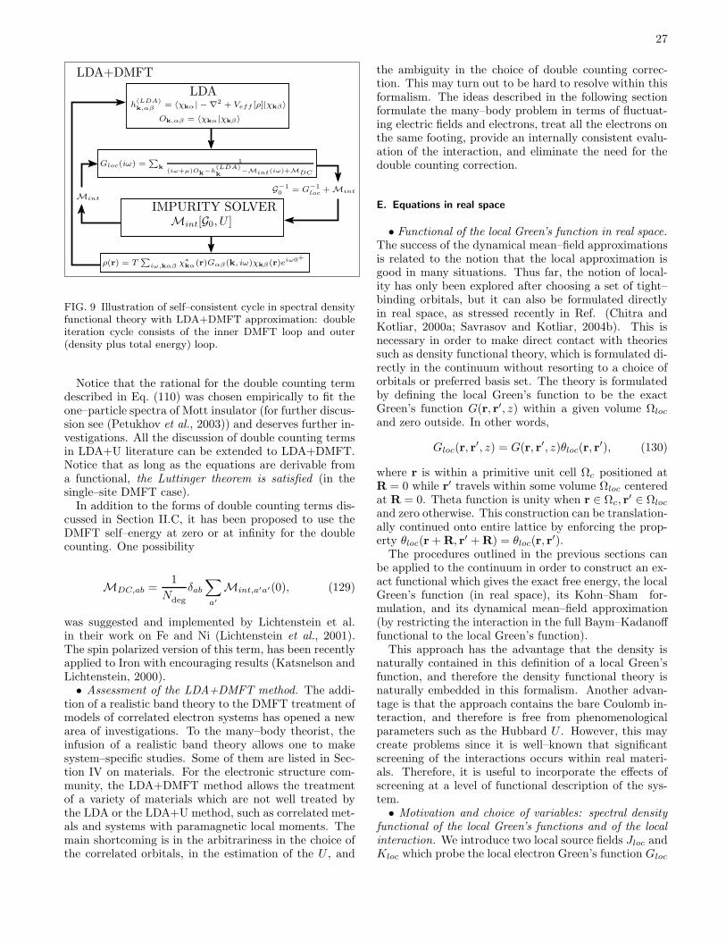
27

Ok,αβ = 〈χkα|χkβ〉

h(LDA)k,αβ = 〈χkα| − ∇2 + Veff [ρ]|χkβ〉

LDA

IMPURITY SOLVERMint[G0, U ]

Gloc(iω) =P

k

1

(iω+µ)Ok−h

(LDA)k

−Mint(iω)+MDC

ρ(r) = TP

iω,kαβ χ∗kα(r)Gαβ(k, iω)χkβ (r)eiω0+

G−10 = G−1

loc + MintMint

LDA+DMFT

FIG. 9 Illustration of self–consistent cycle in spectral densityfunctional theory with LDA+DMFT approximation: doubleiteration cycle consists of the inner DMFT loop and outer(density plus total energy) loop.

Notice that the rational for the double counting termdescribed in Eq. (110) was chosen empirically to fit theone–particle spectra of Mott insulator (for further discus-sion see (Petukhov et al., 2003)) and deserves further in-vestigations. All the discussion of double counting termsin LDA+U literature can be extended to LDA+DMFT.Notice that as long as the equations are derivable froma functional, the Luttinger theorem is satisfied (in thesingle–site DMFT case).

In addition to the forms of double counting terms dis-cussed in Section II.C, it has been proposed to use theDMFT self–energy at zero or at infinity for the doublecounting. One possibility

MDC,ab =1

Ndeg

δab

∑

a′

Mint,a′a′(0), (129)

was suggested and implemented by Lichtenstein et al.in their work on Fe and Ni (Lichtenstein et al., 2001).The spin polarized version of this term, has been recentlyapplied to Iron with encouraging results (Katsnelson andLichtenstein, 2000).• Assessment of the LDA+DMFT method. The addi-

tion of a realistic band theory to the DMFT treatment ofmodels of correlated electron systems has opened a newarea of investigations. To the many–body theorist, theinfusion of a realistic band theory allows one to makesystem–specific studies. Some of them are listed in Sec-tion IV on materials. For the electronic structure com-munity, the LDA+DMFT method allows the treatmentof a variety of materials which are not well treated bythe LDA or the LDA+U method, such as correlated met-als and systems with paramagnetic local moments. Themain shortcoming is in the arbitrariness in the choice ofthe correlated orbitals, in the estimation of the U , and

the ambiguity in the choice of double counting correc-tion. This may turn out to be hard to resolve within thisformalism. The ideas described in the following sectionformulate the many–body problem in terms of fluctuat-ing electric fields and electrons, treat all the electrons onthe same footing, provide an internally consistent evalu-ation of the interaction, and eliminate the need for thedouble counting correction.

E. Equations in real space

• Functional of the local Green’s function in real space.The success of the dynamical mean–field approximationsis related to the notion that the local approximation isgood in many situations. Thus far, the notion of local-ity has only been explored after choosing a set of tight–binding orbitals, but it can also be formulated directlyin real space, as stressed recently in Ref. (Chitra andKotliar, 2000a; Savrasov and Kotliar, 2004b). This isnecessary in order to make direct contact with theoriessuch as density functional theory, which is formulated di-rectly in the continuum without resorting to a choice oforbitals or preferred basis set. The theory is formulatedby defining the local Green’s function to be the exactGreen’s function G(r, r′, z) within a given volume Ωloc

and zero outside. In other words,

Gloc(r, r′, z) = G(r, r′, z)θloc(r, r

′), (130)

where r is within a primitive unit cell Ωc positioned atR = 0 while r′ travels within some volume Ωloc centeredat R = 0. Theta function is unity when r ∈ Ωc, r

′ ∈ Ωloc

and zero otherwise. This construction can be translation-ally continued onto entire lattice by enforcing the prop-erty θloc(r + R, r′ + R) = θloc(r, r

′).The procedures outlined in the previous sections can

be applied to the continuum in order to construct an ex-act functional which gives the exact free energy, the localGreen’s function (in real space), its Kohn–Sham for-mulation, and its dynamical mean–field approximation(by restricting the interaction in the full Baym–Kadanofffunctional to the local Green’s function).

This approach has the advantage that the density isnaturally contained in this definition of a local Green’sfunction, and therefore the density functional theory isnaturally embedded in this formalism. Another advan-tage is that the approach contains the bare Coulomb in-teraction, and therefore is free from phenomenologicalparameters such as the Hubbard U . However, this maycreate problems since it is well–known that significantscreening of the interactions occurs within real materi-als. Therefore, it is useful to incorporate the effects ofscreening at a level of functional description of the sys-tem.• Motivation and choice of variables: spectral density

functional of the local Green’s functions and of the localinteraction. We introduce two local source fields Jloc andKloc which probe the local electron Green’s function Gloc

28

defined earlier and the local part of the boson Green’sfunction Wloc(x, x

′) = 〈Tτφ(x)φ(x′)〉θloc(r, r′) being the

screened interaction (see Section I.B.3). This general-ization represents the ideas of the extended dynamicalmean–field theory (Si and Smith, 1996), now viewed asan exact theory. Note that formally the cluster for theinteraction can be different from the one considered todefine the local Green’s function (130) but we will notdistinguish between them for simplicity. The auxiliary

Green’s function G(r, r′, iω) as well as the auxiliary inter-action W(r, r′, iω) are introduced which are the same asthe local functions within non–zero volume of θloc(r, r

′)

Gloc(r, r′, iω) = G(r, r′, iω)θloc(r, r

′), (131)

Wloc(r, r′, iω) = W(r, r′, iω)θloc(r, r

′). (132)

The spectral density functional is represented in the form

ΓSDFT [Gloc,Wloc] = Tr lnG −Tr[G−10 −G−1]G+EH [ρ]− 1

2Tr lnW +

1

2Tr[v−1

C −W−1]W +ΨSDFT [Gloc,Wloc]. (133)

It can be viewed as a functional ΓSDFT [Gloc,Wloc]or alternatively as a functional ΓSDFT [G,W ].ΨSDFT [Gloc,Wloc] is formally not a sum of two–particle diagrams constructed with Gloc and Wloc, but inprinciple a more complicated diagrammatic expressioncan be derived following Refs. (Chitra and Kotliar,2001; Fukuda et al., 1994; Valiev and Fernando, 1997).A more explicit expression involving a coupling constantintegration can be given. Examining stationarity ofΓSDFT yields saddle–point equations for G(r, r′, iω) andfor W(r, r′, iω)

G−1(r, r′, iω) = G−10 (r, r′, iω) −Mint(r, r

′, iω), (134)

W−1(r, r′, iω) = v−1C (r − r′) −P(r, r′, iω), (135)

where Mint(r, r′, iω) is the auxiliary local mass operator

defined as the variational derivative of the interactionfunctional:

Mint(r, r′, iω) =

δΦSDFT [Gloc]

δG(r′, r, iω)=δΦSDFT [Gloc]

δGloc(r′, r, iω)θloc(r, r

′),

(136)P(r, r′, iω) is the effective susceptibility of the systemdefined as the variational derivative

P(r, r′, iω) =−2δΨSDFT

δW(r′, r, iω)=

−2δΨSDFT

δWloc(r′, r, iω)θloc(r, r

′).

(137)

Notice again a set of parallel observations for P as forMint. Both P and Mint are local by construction, i.e.these are non–zero only within the cluster restricted byθloc(r, r

′). Formally, they are auxiliary objects and can-not be identified with the exact self–energy and suscep-tibility of the electronic system. However, if the ex-act self–energy and susceptibility are sufficiently local-ized, this identification becomes possible. If the clusterΩloc includes the physical area of localization, we canimmediately identify Mint(r, r

′, iω) with Σint(r, r′, iω),

P(r, r′, iω) with Π(r, r′, iω) in all space. However, bothG(r, r′, iω) and G(r, r′, iω) as well as W and W are al-ways the same within Ωloc regardless its size, as it is seenfrom (131) and (132).• Practical implementation and Kohn–Sham represen-

tation. The Kohn–Sham Green’s function can be calcu-lated using the following representation

G(r, r′, iω) =∑

kj

ψRkjω(r)ψL

kjω(r′)

iω + µ− εkjω, (138)

where the left ψLkjω(r) and right ψR

kjω(r) states satisfythe following Dyson equations

[−∇2 + Vext(r) + VH(r)]ψRkjω(r) +

∫Mxc(r, r

′, iω)ψRkjω(r′)dr′ = εkjωψ

Rkjω(r), (139)

[−∇2 + Vext(r′) + VH(r′)]ψL

kjω(r′) +

∫ψL

kjω(r)Mxc(r, r′, iω)dr = εkjωψ

Lkjω(r′). (140)

These equations should be considered as eigenvalue prob-lems with a complex, non–hermitian self–energy. As a

result, the eigenvalues εkjω are complex in general, andthe same for both equations. The explicit dependence on

29

the frequency iω of both the eigenvectors and eigenval-ues comes from the self–energy. Note that left and righteigenfunctions are orthonormal

∫drψL

kjω(r)ψRkj′ω(r)=δjj′ , (141)

and can be used to evaluate the charge density of a givensystem using the Matsubara sum and the integral overthe momentum space

ρ(r) = T∑

iω

∑

kj

ψRkjω(r)ψL

kjω(r)

iω + µ− εkjωeiω0+

. (142)

It can be shown (Savrasov and Kotliar, 2004b) that thissystem of equations reduces to the Kohn–Sham eigensys-tem when the self–energy is frequency independent.

Note that the frequency–dependent energy bands εkjω

represent an auxiliary set of complex eigenvalues. These

are not the true poles of the exact one–electron Green’sfunction G(r, r′, z). However, they are designed to repro-duce the local spectral density of the system. Note alsothat these bands εkjz are not the true poles of the aux-iliary Green’s function G(r, r′, z). Only in the situationwhen G is a good approximation to G, the solution of theequation z+µ− εkjz = 0 gives a good approximation forthe quasiparticle energies

• Evaluation of the total energy. The energy–dependent representation allows one to obtain a verycompact expression for the total energy. As we have ar-gued, the entropy terms are more difficult to evaluate.However, as long as we stay at low temperatures, thesecontributions are small and the total energy approach isvalid. In this respect, the SDFT total energy formulais obtained by utilizing the relationship εkjω = 〈ψL

kjω | −∇2+Meff |ψR

kjω〉 = 〈ψLkjω |−∇2+Vext +VH +Mxc|ψR

kjω〉

ESDFT = T∑

iω

eiω0+ ∑

kj

gkjωεkjω − T∑

iω

∫drdr′Meff (r, r′, iω)G(r′, r, iω) +

+

∫drVext(r)ρ(r) +EH [ρ] +

1

2T∑

iω

∫drdr′Mxc(r, r

′, iω)Gloc(r′, r, iω), (143)

where Meff = Mint + Vext and gkjω = 1/(iω + µ −εkjω). For the same reason as in DFT, this expressionshould be evaluated with the value of the the self-energyMeff which is used as input to the routine performingthe inversion of the Dyson equation, and with the valueof the Green’s function G which is the output of thatinversion.• Constructions of approximations. The dynamical

mean–field approximation to the exact spectral den-sity functional is defined by restricting the interactionpart of Baym–Kadanoff functional ΨSDFT [Gloc,Wloc] toGloc(r, r

′, z) and Wloc(r, r′, iω). The sum over all the di-

agrams, constrained to a given site, together with theDyson equations can be formulated in terms of the so-lution of an auxiliary Anderson impurity model, afterthe introduction of a basis set. We introduce a bathGreen’s function G0(r, r

′, iω) and a “bath interaction”V0(r, r

′, iω) defined by the following Dyson equations

G−10 (r, r′, iω) = G−1

loc(r, r′, iω) + Mint(r, r

′, iω), (144)

V−10 (r, r′, iω) = W−1

loc (r, r′, iω) + P(r, r′, iω). (145)

Note that formally neither G0 nor V0 can be associatedwith non–interacting G0 and the bare interaction vC , re-spectively. These two functions are to be considered asan input to the auxiliary impurity model which deliversnew Mint(r, r

′, iω) and P(r, r′, iω).To summarize, the effective impurity action, the Dyson

equations (144), (145) connecting local and bath quanti-ties as well as the original Dyson equations (134), (135)constitute a self–consistent set of equations as the saddle–point conditions extremizing the spectral density func-tional ΓSDFT (G,W). They combine cellular and ex-tended versions of DMFT and represent our philosophy inthe ab initio simulation of a strongly–correlated system.Since Mint and P are unknown at the beginning, the so-lution of these equations assumes self–consistency. First,assuming some initial Mint and P , the original Dysonequations (134), (135) are used to find Green’s functionG and screened interaction W . Second, the Dyson equa-tions for the local quantities (144), (145) are used to findG0, V0. Third, quantum impurity model with input G0, V0

is solved by available many–body technique to give newlocal Mint and P : this is a much more challenging taskthan purely fermionic calculations (e.g. cluster DMFT inHubbard model), which can only be addressed at presentwith Quantum Monte Carlo methods using continuousHubbard-Stratonovich fields (Sun and Kotliar, 2002) orpossibly with continuous Quantum Monte Carlo studiedin (Rubtsov et al., 2004). The process is repeated untilself–consistency is reached. This is schematically illus-trated in Fig. 10. Note here that while single–site im-purity problem has a well–defined algorithm to extractthe lattice self–energy, this is not generally true for thecluster impurity models (Biroli et al., 2004). The latter

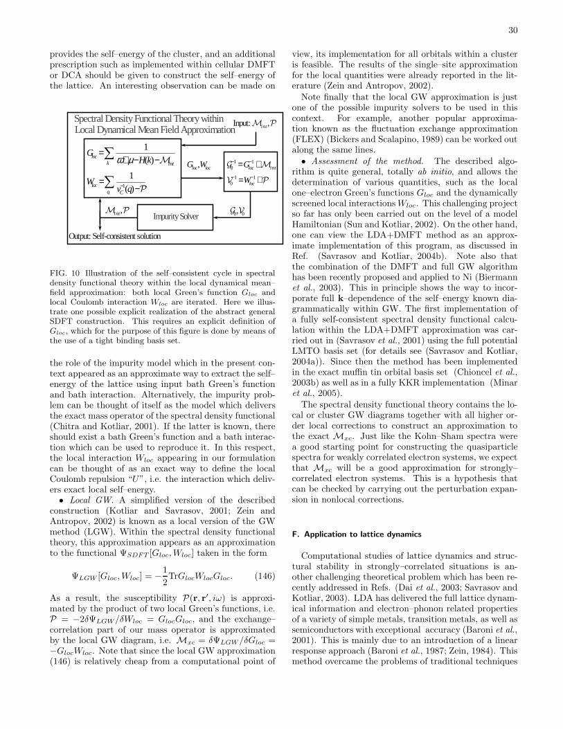
30

provides the self–energy of the cluster, and an additionalprescription such as implemented within cellular DMFTor DCA should be given to construct the self–energy ofthe lattice. An interesting observation can be made on

1 10

1 10

loc

loc

G

W

− −

− −

= +

= +

1

1

( )

1

( )

lock

locq C

GH k

Wv q

ω

−

=+ −

=−

∑∑

0 0

,,int

Local Impurity Model

Input: ,

Output: Self-consistent solution

Spectral Density Functional Theory withinLocal Dynamical Mean Field Approximation

,loc locG W 1 10

1 10

loc int

loc

G

W

− −

− −

= +

= +

G MV P

1

1

( )

1

( )

lock int

locq C

GH k

Wv q

ω µ

−

=+ − −

=−

∑∑

M

P

0 0G V,,intM PImpurity Solver

Input: ,intM P

Output: Self-consistent solution

Spectral Density Functional Theory withinLocal Dynamical Mean Field Approximation

FIG. 10 Illustration of the self–consistent cycle in spectraldensity functional theory within the local dynamical mean–field approximation: both local Green’s function Gloc andlocal Coulomb interaction Wloc are iterated. Here we illus-trate one possible explicit realization of the abstract generalSDFT construction. This requires an explicit definition ofGloc, which for the purpose of this figure is done by means ofthe use of a tight binding basis set.

the role of the impurity model which in the present con-text appeared as an approximate way to extract the self–energy of the lattice using input bath Green’s functionand bath interaction. Alternatively, the impurity prob-lem can be thought of itself as the model which deliversthe exact mass operator of the spectral density functional(Chitra and Kotliar, 2001). If the latter is known, thereshould exist a bath Green’s function and a bath interac-tion which can be used to reproduce it. In this respect,the local interaction Wloc appearing in our formulationcan be thought of as an exact way to define the localCoulomb repulsion “U”, i.e. the interaction which deliv-ers exact local self–energy.• Local GW. A simplified version of the described

construction (Kotliar and Savrasov, 2001; Zein andAntropov, 2002) is known as a local version of the GWmethod (LGW). Within the spectral density functionaltheory, this approximation appears as an approximationto the functional ΨSDFT [Gloc,Wloc] taken in the form

ΨLGW [Gloc,Wloc] = −1

2TrGlocWlocGloc. (146)

As a result, the susceptibility P(r, r′, iω) is approxi-mated by the product of two local Green’s functions, i.e.P = −2δΨLGW/δWloc = GlocGloc, and the exchange–correlation part of our mass operator is approximatedby the local GW diagram, i.e. Mxc = δΨLGW/δGloc =−GlocWloc. Note that since the local GW approximation(146) is relatively cheap from a computational point of

view, its implementation for all orbitals within a clusteris feasible. The results of the single–site approximationfor the local quantities were already reported in the lit-erature (Zein and Antropov, 2002).

Note finally that the local GW approximation is justone of the possible impurity solvers to be used in thiscontext. For example, another popular approxima-tion known as the fluctuation exchange approximation(FLEX) (Bickers and Scalapino, 1989) can be worked outalong the same lines.• Assessment of the method. The described algo-

rithm is quite general, totally ab initio, and allows thedetermination of various quantities, such as the localone–electron Green’s functions Gloc and the dynamicallyscreened local interactionsWloc. This challenging projectso far has only been carried out on the level of a modelHamiltonian (Sun and Kotliar, 2002). On the other hand,one can view the LDA+DMFT method as an approx-imate implementation of this program, as discussed inRef. (Savrasov and Kotliar, 2004b). Note also thatthe combination of the DMFT and full GW algorithmhas been recently proposed and applied to Ni (Biermannet al., 2003). This in principle shows the way to incor-porate full k–dependence of the self–energy known dia-grammatically within GW. The first implementation ofa fully self-consistent spectral density functional calcu-lation within the LDA+DMFT approximation was car-ried out in (Savrasov et al., 2001) using the full potentialLMTO basis set (for details see (Savrasov and Kotliar,2004a)). Since then the method has been implementedin the exact muffin tin orbital basis set (Chioncel et al.,2003b) as well as in a fully KKR implementation (Minaret al., 2005).

The spectral density functional theory contains the lo-cal or cluster GW diagrams together with all higher or-der local corrections to construct an approximation tothe exact Mxc. Just like the Kohn–Sham spectra werea good starting point for constructing the quasiparticlespectra for weakly correlated electron systems, we expectthat Mxc will be a good approximation for strongly–correlated electron systems. This is a hypothesis thatcan be checked by carrying out the perturbation expan-sion in nonlocal corrections.

F. Application to lattice dynamics

Computational studies of lattice dynamics and struc-tural stability in strongly–correlated situations is an-other challenging theoretical problem which has been re-cently addressed in Refs. (Dai et al., 2003; Savrasov andKotliar, 2003). LDA has delivered the full lattice dynam-ical information and electron–phonon related propertiesof a variety of simple metals, transition metals, as well assemiconductors with exceptional accuracy (Baroni et al.,2001). This is mainly due to an introduction of a linearresponse approach (Baroni et al., 1987; Zein, 1984). Thismethod overcame the problems of traditional techniques

31

based on static susceptibility calculations which gener-ally fail to reproduce lattice dynamical properties of realmaterials due to difficulties connected with the summa-tions in high–energy states and the inversion of very largedielectric matrix (J. T. Devreese and Camp, 1983).

Despite these impressive successes, there is by nowclear evidence that the present methodology fails whenapplied to strongly–correlated materials. For example,the local density predictions for such properties as bulkmodulus and elastic constants in metallic Plutonium areapproximately one order of magnitude off from exper-iment (Bouchet et al., 2000); the phonon spectrum ofMott insulators such as MnO is not predicted correctlyby LDA (Massidda et al., 1999).

Recently, a linear response method to study the lat-tice dynamics of correlated materials has been developed(Dai et al., 2003; Savrasov and Kotliar, 2003). The dy-namical matrix being the second order derivative of theenergy can be computed using spectral density functionaltheory. As with the ordinary density functional formu-lation of the problem (Savrasov, 1996), we deal with thefirst order corrections to the charge density, δρ, as well asthe first order correction to the Green’s function δG(iω)which should be considered as two independent variablesin the functional of the dynamical matrix. To find theextremum, a set of the linearized Dyson equations has tobe solved self–consistently

[−∇2+Meff (iω)−εkjω]δψRkjω+[δMeff (iω)−δεkjω]ψR

kjω = 0,(147)

which leads us to consider the first order changes in thelocal mass operator Meff (iω). Here and in the follow-ing we will assume that the phonon wave vector of theperturbation q is different from zero, and, therefore, thefirst order changes in the eigenvalues δεkjω drop out. The

quantity δMeff (iω) is a functional of δG(iω) and shouldbe found self–consistently. In particular, the change inthe self–energy δMeff (iω) needs a solution of an AIMlinearized with respect to the atomic displacement, whichin practice requires the computation of a two-particle ver-tex function Γ = δ2ΦSDFT (Gloc)/(δGlocδGloc).

In practice, change in the eigenvector δψkjω has tobe expanded in some basis set. Previous linear responseschemes were based on tight–binding methods (Varmaand Weber, 1977), plane wave pseudopotentials (Ba-roni et al., 1987; Gonze et al., 1992; Quong and Klein,1992; Zein, 1984), linear augmented plane waves(Yu andKrakauer, 1994), mixed orbitals (Heid and Bohnen, 1999)and linear muffin–tin orbitals (Savrasov, 1992). Due toexplicit dependence on the atomic positions of local or-bital basis sets both Hellmann–Feynman contributionsand incomplete basis set corrections appear in the ex-pression for the dynamical matrix (Savrasov, 1996). Thefunctions δψkjω are represented as follows

δψkjω =∑

α

δAkjωα χk+q

α +Akjωα δχk

α, (148)

where we introduced both changes in the frequency–dependent variational coefficients δAkjω

α as well as

changes in the basis functions δχkα. The latter helps us to

reach fast convergence in the entire expression (148) withrespect to the number of the basis functions α since thecontribution with δχk

α takes into account all rigid move-ments of the localized orbitals (Savrasov, 1992).

FIG. 11 Illustration of the self–consistent cycle to calculatelattice dynamics within the spectral density functional theory.

The first–order changes in the Green’s function can befound as follows

δGloc(iω) =∑

kj

δψLkjωψ

Rkjω + ψL

kjωδψRkjω

iω + µ− εkjω, (149)

which should be used to evaluate the first order change inthe charge density and the dynamical matrix itself (seeFig. 11).

A simplified version of the approach, neglecting theimpurity vertex function, was successfully applied to theparamagnetic phases of Mott insulators (Savrasov andKotliar, 2003) as well as to high–temperature phases ofPlutonium (Dai et al., 2003). We will describe these ap-plications in Section IV.

G. Application to optics and transport

Optical spectral functions such as conductivity or re-flectivity are very important characteristics of solids andgive us a direct probe of the electronic structure.

Here we outline an approach which allows to calcu-late the optical properties of a strongly–correlated ma-terial within the spectral density functional framework(Oudovenko et al., 2004b; Perlov et al., 2004). This workextends the methodology in use for weak correlated sys-tems (see (Maksimov et al., 1988)) to correlated materi-als. The optical conductivity can be expressed via equi-librium state current–current correlation function (Ma-

32

han, 1993) and is given by

σµν(ω) = (150)

πe2+∞∫

−∞

dεφµν(ε+ ω/2, ε− ω/2)f(ε− ω/2)−f(ε+ ω/2)

ω,

where f(ε) is the Fermi function, and the transport func-tion φµν(ε, ε′) is

φµν(ε, ε′) =1

Ωc

∑

kjj′

Tr∇µρkj(ε)∇νρkj′(ε

′), (151)

where Ωc is the unit cell volume and

ρkj(ε) = − 1

2πi

(Gkj(ε) − G†

kj(ε)), (152)

is expressed via retarded one–particle Green’s function,Gkj(ε), of the system. Taking limit of zero temperature

and using the solutions εkjω and ψR,Lkjω of the Dyson equa-

tion (139), (140) on the real frequency axis we express theoptical conductivity in the form

σµν(ω) =πe2

ω

∑

ss′=±

ss′∑

kjj′

+ω/2∫

−ω/2

dεMss′,µν

kjj′ (ε−, ε+)

ω + εskjε− − εs

′

kj′ε+

[1

ε− + µ− εskjε−

− 1

ε+ + µ− εs′

kj′ε+

], (153)

where we have denoted ε± = ε ± ω/2, and used the ab-breviated notations ε+kjε ≡ εkjε, ε

−kjε = ε∗kjε.

The matrix elements Mkjj′ are generalizations of thestandard dipole allowed transition probabilities which arenow defined with the right and left solutions ψRand ψL

of the Dyson equation

Mss′,µνkjj′ (ε, ε′) = (154)

∫(ψs

kjε)s∇µ(ψ−s′

kjε′ )s′

dr

∫(ψs′

kj′ε′)s′∇ν(ψ−skjε)

sdr,

where we have denoted ψ+kjε = ψL

kjε , ψ−kjε = ψR

kjε and

assumed that (ψskjε)

+ ≡ ψskjε while (ψs

kjε)− = ψs∗

kjε.

The expressions (153), (155) represent generalizationsof the formulae for optical conductivity for a strongly–correlated system, and involve the extra internal fre-quency integral in Eq. (153).

Let us consider the non–interacting limit whenMxc(ω) → iγ → 0. In this case, the eigenvalues εkjε =εkj + iγ, ψR

kjε ≡ |kj〉, ψLkjε ≡ |kj〉∗ ≡ 〈kj| and the matrix

elements M ss′,µνkjj′ (ε, ε′) are all expressed via the standard

dipole transitions |〈kj|∇|kj ′〉|2. Working out the energydenominators in the expression (153) in the limit iγ → 0and for ω 6= 0 leads us to the usual form for the conduc-tivity which for its interband contribution has the form

σµν(ω) =πe2

ω

∑

k,j′ 6=j

〈kj|∇µ|kj′〉〈kj′|∇ν |kj〉 ×

[f(εkj) − f(εkj′)]δ(εkj − εkj′ + ω). (155)

To evaluate the expression σµν (ω) numerically, oneneeds to pay special attention to the energy denomina-tor 1/(ω + εs

kjε− − εs′

kj′ε+) in (153). Due to its strong

k-dependence the tetrahedron method of Lambin andVigneron (Lambin and Vigneron, 1984) should be used.

On the other hand, the difference in the square brack-ets of Eq. (153) is a smooth function of k and one canevaluate it using linear interpolation. This allows oneto calculate the integral over ε by dividing the inter-val −ω/2 < ε < +ω/2 into discrete set of points εi

and assuming that the eigenvalues εkjε and eigenvec-tors ψkjε can to zeroth order be approximated by theirvalues at the middle between each pair of points i.e.ε±i = εi ±ω/2+ (εi+1− εi)/2. In this way, the integral isreplaced by the discrete sum over internal grid εi definedfor each frequency ω, and the Dyson equation needs tobe solved twice for the energy ε+i and for the energy ε−iThe described procedure produces fast and accurate al-gorithm for evaluating the optical response functions ofa strongly–correlated material.

Similar developments can be applied to calculate thetransport properties such as dc-resistivity. The trans-port parameters of the system are expressed in terms ofso called kinetic coefficient, denoted here by Am. Theequation for the electrical resistivity is given by

ρ =kBT

e21

A0, (156)

and the thermopower and the thermal conductivity aregiven by

S =−kB

|e|A1

A0, κ = kB

(A2 −

A21

A0

). (157)

Within the Kubo formalism (Mahan, 1993) the ki-netic coefficients are given in terms of equilibrium statecurrent–current correlation functions of the particle andthe heat current in the system. To evaluate these correla-tion functions an expression for electric and heat currentsare needed. Once those currents are evaluated, transportwith DMFT reduces to the evaluation of the transport

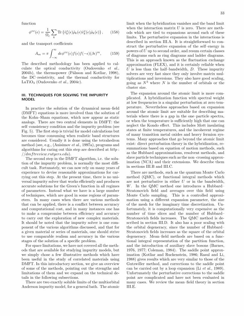
33

function

φxx(ε) =1

Ωc

∑

k

Tr vxk (ε)ρk(ε)vx

k (ε)ρk(ε) , (158)

and the transport coefficients

Am = π

∫ ∞

−∞

dεφxx(ε)f(ε)f(−ε)(βε)m, (159)

The described methodology has been applied to cal-culate the optical conductivity (Oudovenko et al.,2004b), the thermopower (Palsson and Kotliar, 1998),the DC–resistivity, and the thermal conductivity forLaTiO3 (Oudovenko et al., 2004c).

III. TECHNIQUES FOR SOLVING THE IMPURITY

MODEL

In practice the solution of the dynamical mean–field(DMFT) equations is more involved than the solution ofthe Kohn–Sham equations, which now appear as staticanalogs. There are two central elements in DMFT: theself–consistency condition and the impurity problem (seeFig. 5). The first step is trivial for model calculations butbecomes time consuming when realistic band structuresare considered. Usually it is done using the tetrahedronmethod (see, e.g., (Anisimov et al., 1997a), programs andalgorithms for caring out this step are described at http ://dmftreview.rutgers.edu).

The second step in the DMFT algorithm, i.e. the solu-tion of the impurity problem, is normally the most diffi-cult task. Fortunately, we can now rely on many years ofexperience to devise reasonable approximations for car-rying out this step. At the present time, there is no uni-versal impurity solver that works efficiently and producesaccurate solutions for the Green’s function in all regimesof parameters. Instead what we have is a large numberof techniques, which are good in some regions of param-eters. In many cases when there are various methodsthat can be applied, there is a conflict between accuracyand computational cost, and in many instances one hasto make a compromise between efficiency and accuracyto carry out the exploration of new complex materials.It should be noted that the impurity solver is one com-ponent of the various algorithms discussed, and that fora given material or series of materials, one should striveto use comparable realism and accuracy in the variousstages of the solution of a specific problem.

For space limitations, we have not covered all the meth-ods that are available for studying impurity models, butwe simply chose a few illustrative methods which havebeen useful in the study of correlated materials usingDMFT. In this introductory section, we give an overviewof some of the methods, pointing out the strengths andlimitations of them and we expand on the technical de-tails in the following subsections.

There are two exactly soluble limits of the multiorbitalAnderson impurity model, for a general bath. The atomic

limit when the hybridization vanishes and the band limitwhen the interaction matrix U is zero. There are meth-ods which are tied to expansions around each of theselimits. The perturbative expansion in the interactions isdescribed in section III.A. It is straightforward to con-struct the perturbative expansion of the self–energy inpowers of U up to second order, and resum certain classesof diagrams such as ring diagrams and ladder diagrams.This is an approach known as the fluctuation exchangeapproximation (FLEX), and it is certainly reliable whenU is less than the half–bandwidth, D. These impuritysolvers are very fast since they only involve matrix mul-tiplications and inversions. They also have good scaling,going as N3 where N is the number of orbitals or thecluster size.

The expansion around the atomic limit is more com-plicated. A hybridization function with spectral weightat low frequencies is a singular perturbation at zero tem-perature. Nevertheless approaches based on expansionaround the atomic limit are suitable for describing ma-terials where there is a gap in the one–particle spectra,or when the temperature is sufficiently high that one canneglect the Kondo effect. This includes Mott insulatingstates at finite temperatures, and the incoherent regimeof many transition metal oxides and heavy fermion sys-tems. Many approaches that go beyond the atomic limitexist: direct perturbation theory in the hybridization, re-summations based on equation of motion methods, suchas the Hubbard approximations, resolvent methods, andslave particle techniques such as the non–crossing approx-imation (NCA) and their extensions. We describe themin sections III.B and III.C.

There are methods, such as the quantum Monte Carlomethod (QMC), or functional integral methods whichare not perturbative in either U or in the bandwidth,W . In the QMC method one introduces a Hubbard–Stratonovich field and averages over this field usingMonte Carlo sampling. This is a controlled approxi-mation using a different expansion parameter, the sizeof the mesh for the imaginary time discretization. Un-fortunately, it is computationally very expensive as thenumber of time slices and the number of Hubbard–Stratonovich fields increases. The QMC method is de-scribed in section III.D. It also has a poor scaling withthe orbital degeneracy, since the number of Hubbard–Stratonovich fields increases as the square of the orbitaldegeneracy. Mean–field methods are based on a func-tional integral representation of the partition function,and the introduction of auxiliary slave bosons (Barnes,1976, 1977; Coleman, 1984). The saddle point approx-imation (Kotliar and Ruckenstein, 1986; Rasul and Li,1988) gives results which are very similar to those of theGutzwiller method, and corrections to the saddle pointcan be carried out by a loop expansion (Li et al., 1989).Unfortunately the perturbative corrections to the saddlepoint are complicated and have not been evaluated inmany cases. We review the mean–field theory in sectionIII.E.

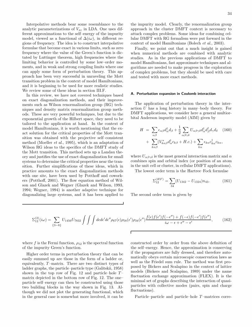
34

Interpolative methods bear some resemblance to theanalytic parameterizations of Vxc in LDA. One uses dif-ferent approximations to the self–energy of the impuritymodel, viewed as a functional of ∆(iω), in different re-gions of frequency. The idea is to construct interpolativeformulae that become exact in various limits, such as zerofrequency where the value of the Green’s function is dic-tated by Luttinger theorem, high frequencies where thelimiting behavior is controlled by some low–order mo-ments, and in weak and strong coupling limits where onecan apply some form of perturbation theory. This ap-proach has been very successful in unraveling the Motttransition problem in the context of model Hamiltonians,and it is beginning to be used for more realistic studies.We review some of these ideas in section III.F.

In this review, we have not covered techniques basedon exact diagonalization methods, and their improve-ments such as Wilson renormalization group (RG) tech-niques and density matrix renormalization group meth-ods. These are very powerful techniques, but due to theexponential growth of the Hilbert space, they need to betailored to the application at hand. In the context ofmodel Hamiltonians, it is worth mentioning that the ex-act solution for the critical properties of the Mott tran-sition was obtained with the projective self–consistentmethod (Moeller et al., 1995), which is an adaptation ofWilson RG ideas to the specifics of the DMFT study ofthe Mott transition. This method sets up a Landau the-ory and justifies the use of exact diagonalization for smallsystems to determine the critical properties near the tran-sition. Further simplifications of these ideas, which inpractice amounts to the exact diagonalization methodswith one site, have been used by Potthoff and cowork-ers (Potthoff, 2001). The flow equation method of Wil-son and Glazek and Wegner (Glazek and Wilson, 1993,1994; Wegner, 1994) is another adaptive technique fordiagonalizing large systems, and it has been applied to

the impurity model. Clearly, the renormalization groupapproach in the cluster DMFT context is necessary toattack complex problems. Some ideas for combining cel-lular DMFT with RG formalism were put forward in thecontext of model Hamiltonians (Bolech et al., 2003).

Finally, we point out that a much insight is gainedwhen numerical methods are combined with analyticstudies. As in the previous applications of DMFT tomodel Hamiltonians, fast approximate techniques and al-gorithms are needed to make progress in the explorationof complex problems, but they should be used with careand tested with more exact methods.

A. Perturbation expansion in Coulomb interaction

The application of perturbation theory in the inter-action U has a long history in many–body theory. ForDMFT applications, we consider here a general multior-bital Anderson impurity model (AIM) given by

H =∑

αβ

εαβd†αdβ +

1

2

∑

αβγδ

Uαβγδd†αd

†βdγdδ (160)

+∑

kαβ

(V ∗kαβd

†αckβ +H.c.) +

∑

kα

εkαc†kαckα,

where Uαβγδ is the most general interaction matrix and αcombines spin and orbital index (or position of an atomin the unit cell or cluster, in cellular DMFT applications).

The lowest order term is the Hartree–Fock formulae

Σ(HF )12 =

∑

34

(U1342 − U1324)n43. (161)

The second order term is given by

Σ(2)12 (iω) =

∑

3−8

U1456U7832

∫ ∫ ∫dεdε′dε′′ρ67(ε)ρ58(ε

′)ρ34(ε′′)f(ε)f(ε′)f(−ε′′) + f(−ε)f(−ε′)f(ε′′)

iω − ε+ ε′′ − ε′, (162)

where f is the Fermi function, ρ12 is the spectral functionof the impurity Green’s function.

Higher order terms in perturbation theory that can beeasily summed up are those in the form of a ladder or,equivalently, T–matrix. There are two distinct types ofladder graphs, the particle–particle type (Galitskii, 1958)shown in the top row of Fig. 12 and particle–hole T–matrix depicted in the bottom row of Fig. 12. The one–particle self–energy can then be constructed using thosetwo building blocks in the way shown in Fig. 13. Al-though we did not plot the generating functional, whichin the general case is somewhat more involved, it can be

constructed order by order from the above definition ofthe self–energy. Hence, the approximation is conservingif the propagators are fully dressed, and therefore auto-matically obeys certain microscopic conservation laws aswell as the Friedel sum rule. The method was first pro-posed by Bickers and Scalapino in the context of latticemodels (Bickers and Scalapino, 1989) under the namefluctuation exchange approximation (FLEX). It is theminimal set of graphs describing the interaction of quasi-particles with collective modes (pairs, spin and chargefluctuations).

Particle–particle and particle–hole T–matrices corre-

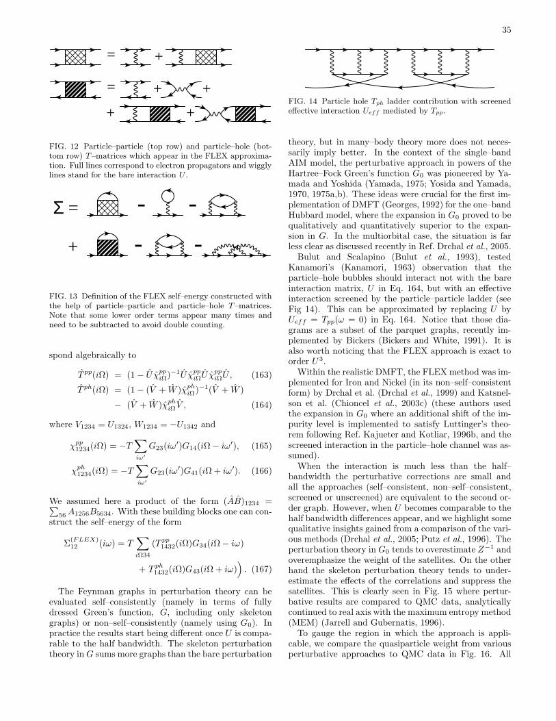
35

= +

= + +

+ +

FIG. 12 Particle–particle (top row) and particle–hole (bot-tom row) T–matrices which appear in the FLEX approxima-tion. Full lines correspond to electron propagators and wigglylines stand for the bare interaction U .

Σ = - -

+ - -

FIG. 13 Definition of the FLEX self–energy constructed withthe help of particle–particle and particle–hole T–matrices.Note that some lower order terms appear many times andneed to be subtracted to avoid double counting.

spond algebraically to

T pp(iΩ) = (1 − U χppiΩ)−1U χpp

iΩU χppiΩU , (163)

T ph(iΩ) = (1 − (V + W )χphiΩ)−1(V + W )

− (V + W )χphiΩ V , (164)

where V1234 = U1324, W1234 = −U1342 and

χpp1234(iΩ) = −T

∑

iω′

G23(iω′)G14(iΩ − iω′), (165)

χph1234(iΩ) = −T

∑

iω′

G23(iω′)G41(iΩ + iω′). (166)

We assumed here a product of the form (AB)1234 =∑56A1256B5634. With these building blocks one can con-

struct the self–energy of the form

Σ(FLEX)12 (iω) = T

∑

iΩ34

(T pp1432(iΩ)G34(iΩ − iω)

+ T ph1432(iΩ)G43(iΩ + iω)

). (167)

The Feynman graphs in perturbation theory can beevaluated self–consistently (namely in terms of fullydressed Green’s function, G, including only skeletongraphs) or non–self–consistently (namely using G0). Inpractice the results start being different once U is compa-rable to the half bandwidth. The skeleton perturbationtheory inG sums more graphs than the bare perturbation

FIG. 14 Particle hole Tph ladder contribution with screenedeffective interaction Ueff mediated by Tpp.

theory, but in many–body theory more does not neces-sarily imply better. In the context of the single–bandAIM model, the perturbative approach in powers of theHartree–Fock Green’s function G0 was pioneered by Ya-mada and Yoshida (Yamada, 1975; Yosida and Yamada,1970, 1975a,b). These ideas were crucial for the first im-plementation of DMFT (Georges, 1992) for the one–bandHubbard model, where the expansion in G0 proved to bequalitatively and quantitatively superior to the expan-sion in G. In the multiorbital case, the situation is farless clear as discussed recently in Ref. Drchal et al., 2005.

Bulut and Scalapino (Bulut et al., 1993), testedKanamori’s (Kanamori, 1963) observation that theparticle–hole bubbles should interact not with the bareinteraction matrix, U in Eq. 164, but with an effectiveinteraction screened by the particle–particle ladder (seeFig 14). This can be approximated by replacing U byUeff = Tpp(ω = 0) in Eq. 164. Notice that those dia-grams are a subset of the parquet graphs, recently im-plemented by Bickers (Bickers and White, 1991). It isalso worth noticing that the FLEX approach is exact toorder U3.

Within the realistic DMFT, the FLEX method was im-plemented for Iron and Nickel (in its non–self–consistentform) by Drchal et al. (Drchal et al., 1999) and Katsnel-son et al. (Chioncel et al., 2003c) (these authors usedthe expansion in G0 where an additional shift of the im-purity level is implemented to satisfy Luttinger’s theo-rem following Ref. Kajueter and Kotliar, 1996b, and thescreened interaction in the particle–hole channel was as-sumed).

When the interaction is much less than the half–bandwidth the perturbative corrections are small andall the approaches (self–consistent, non–self–consistent,screened or unscreened) are equivalent to the second or-der graph. However, when U becomes comparable to thehalf bandwidth differences appear, and we highlight somequalitative insights gained from a comparison of the vari-ous methods (Drchal et al., 2005; Putz et al., 1996). Theperturbation theory in G0 tends to overestimate Z−1 andoveremphasize the weight of the satellites. On the otherhand the skeleton perturbation theory tends to under-estimate the effects of the correlations and suppress thesatellites. This is clearly seen in Fig. 15 where pertur-bative results are compared to QMC data, analyticallycontinued to real axis with the maximum entropy method(MEM) (Jarrell and Gubernatis, 1996).

To gauge the region in which the approach is appli-cable, we compare the quasiparticle weight from variousperturbative approaches to QMC data in Fig. 16. All

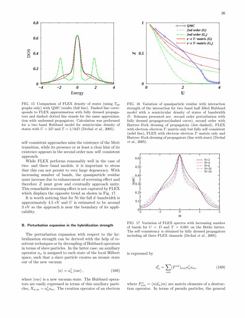
36

−4 −2 0 2 4Energy

0

0.2

0.4

0.6

0.8D

OS

FIG. 15 Comparison of FLEX density of states (using Tpp

graphs only) with QMC results (full line). Dashed line corre-sponds to FLEX approximation with fully dressed propaga-tors and dashed–dotted line stands for the same approxima-tion with undressed propagators. Calculation was performedfor a two–band Hubbard model for semicircular density ofstates with U = 2D and T = 1/16D (Drchal et al., 2005).

self–consistent approaches miss the existence of the Motttransition, while its presence or at least a clear hint of itsexistence appears in the second order non–self–consistentapproach.

While FLEX performs reasonably well in the case oftwo- and three–band models, it is important to stressthat this can not persist to very large degeneracy. Withincreasing number of bands, the quasiparticle residuemust increase due to enhancement of screening effect andtherefore Z must grow and eventually approach unity.This remarkable screening effect is not captured by FLEXwhich displays the opposite trend as shown in Fig. 17.

It is worth noticing that for Ni the full d–bandwidth isapproximately 4.5 eV and U is estimated to be around3 eV so the approach is near the boundary of its appli-cability.

B. Perturbation expansion in the hybridization strength

The perturbation expansion with respect to the hy-bridization strength can be derived with the help of re-solvent techniques or by decoupling of Hubbard operatorsin terms of slave particles. In the latter case, an auxiliaryoperator an is assigned to each state of the local Hilbertspace, such that a slave particle creates an atomic stateout of the new vacuum

|n〉 = a†n |vac〉 , (168)

where |vac〉 is a new vacuum state. The Hubbard opera-tors are easily expressed in terms of this auxiliary parti-cles, Xn,m = a†nam. The creation operator of an electron

0 2 4U

0

0.5

1

Z

QMC2nd order (G)2nd order (G0)e−e T−matrix (G)e−e T−matrix (G0)

FIG. 16 Variation of quasiparticle residue with interactionstrength of the interaction for two–band half–filled Hubbardmodel with a semicircular density of states of bandwidthD. Schemes presented are: second order perturbation withfully dressed propagators(dashed curve), second order withHartree–Fock dressing of propagators (dot–dashed), FLEXwith electron–electron T–matrix only but fully self–consistent(solid line), FLEX with electron–electron T–matrix only andHartree–Fock dressing of propagators (line with stars) (Drchalet al., 2005).

-2 -1 0 1 2ω

0

0.1

0.2

0.3

0.4

0.5

0.6

A(ω

)

N=2N=4N=6N=10N=14

FIG. 17 Variation of FLEX spectra with increasing numberof bands for U = D and T = 0.001 on the Bethe lattice.The self–consistency is obtained by fully dressed propagatorsincluding all three FLEX channels (Drchal et al., 2005).

is expressed by

d†α =∑

nm

(Fα†)nma†nam, (169)

where Fαnm = 〈n|dα|m〉 are matrix elements of a destruc-

tion operator. In terms of pseudo particles, the general

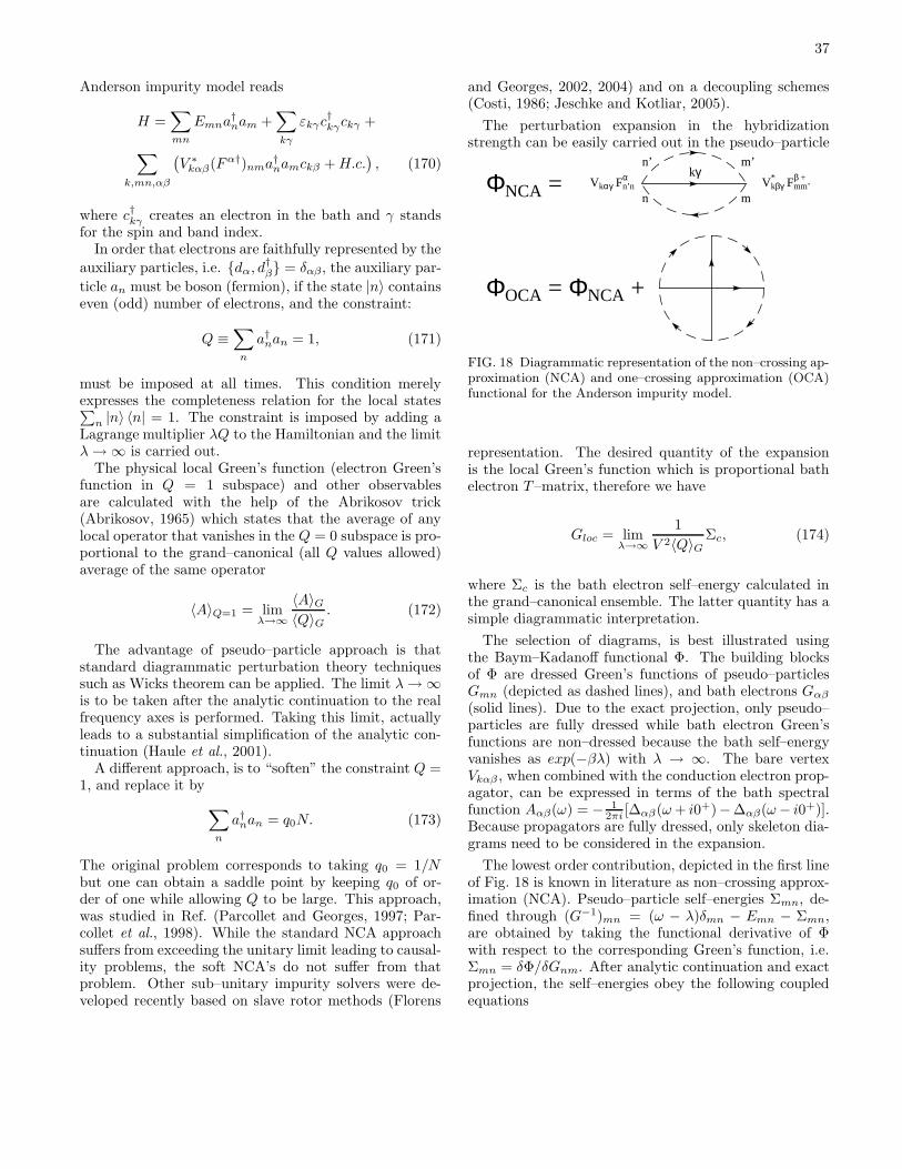
37

Anderson impurity model reads

H =∑

mn

Emna†nam +

∑

kγ

εkγc†kγckγ +

∑

k,mn,αβ

(V ∗

kαβ(Fα†)nma†namckβ +H.c.

), (170)

where c†kγ creates an electron in the bath and γ standsfor the spin and band index.

In order that electrons are faithfully represented by the

auxiliary particles, i.e. dα, d†β = δαβ, the auxiliary par-

ticle an must be boson (fermion), if the state |n〉 containseven (odd) number of electrons, and the constraint:

Q ≡∑

n

a†nan = 1, (171)

must be imposed at all times. This condition merelyexpresses the completeness relation for the local states∑

n |n〉 〈n| = 1. The constraint is imposed by adding aLagrange multiplier λQ to the Hamiltonian and the limitλ→ ∞ is carried out.

The physical local Green’s function (electron Green’sfunction in Q = 1 subspace) and other observablesare calculated with the help of the Abrikosov trick(Abrikosov, 1965) which states that the average of anylocal operator that vanishes in the Q = 0 subspace is pro-portional to the grand–canonical (all Q values allowed)average of the same operator

〈A〉Q=1 = limλ→∞

〈A〉G〈Q〉G

. (172)

The advantage of pseudo–particle approach is thatstandard diagrammatic perturbation theory techniquessuch as Wicks theorem can be applied. The limit λ→ ∞is to be taken after the analytic continuation to the realfrequency axes is performed. Taking this limit, actuallyleads to a substantial simplification of the analytic con-tinuation (Haule et al., 2001).

A different approach, is to “soften” the constraint Q =1, and replace it by

∑

n

a†nan = q0N. (173)

The original problem corresponds to taking q0 = 1/Nbut one can obtain a saddle point by keeping q0 of or-der of one while allowing Q to be large. This approach,was studied in Ref. (Parcollet and Georges, 1997; Par-collet et al., 1998). While the standard NCA approachsuffers from exceeding the unitary limit leading to causal-ity problems, the soft NCA’s do not suffer from thatproblem. Other sub–unitary impurity solvers were de-veloped recently based on slave rotor methods (Florens

and Georges, 2002, 2004) and on a decoupling schemes(Costi, 1986; Jeschke and Kotliar, 2005).

The perturbation expansion in the hybridizationstrength can be easily carried out in the pseudo–particle

ΦNCA = Vkαγ Fαn’n V*

kβγ Fβ +mm’

kγ

n m

n’ m’

ΦOCA = ΦNCA +

FIG. 18 Diagrammatic representation of the non–crossing ap-proximation (NCA) and one–crossing approximation (OCA)functional for the Anderson impurity model.

representation. The desired quantity of the expansionis the local Green’s function which is proportional bathelectron T–matrix, therefore we have

Gloc = limλ→∞

1

V 2〈Q〉GΣc, (174)

where Σc is the bath electron self–energy calculated inthe grand–canonical ensemble. The latter quantity has asimple diagrammatic interpretation.

The selection of diagrams, is best illustrated usingthe Baym–Kadanoff functional Φ. The building blocksof Φ are dressed Green’s functions of pseudo–particlesGmn (depicted as dashed lines), and bath electrons Gαβ

(solid lines). Due to the exact projection, only pseudo–particles are fully dressed while bath electron Green’sfunctions are non–dressed because the bath self–energyvanishes as exp(−βλ) with λ → ∞. The bare vertexVkαβ , when combined with the conduction electron prop-agator, can be expressed in terms of the bath spectralfunction Aαβ(ω) = − 1

2πi [∆αβ(ω+ i0+)−∆αβ(ω− i0+)].Because propagators are fully dressed, only skeleton dia-grams need to be considered in the expansion.

The lowest order contribution, depicted in the first lineof Fig. 18 is known in literature as non–crossing approx-imation (NCA). Pseudo–particle self–energies Σmn, de-fined through (G−1)mn = (ω − λ)δmn − Emn − Σmn,are obtained by taking the functional derivative of Φwith respect to the corresponding Green’s function, i.e.Σmn = δΦ/δGnm. After analytic continuation and exactprojection, the self–energies obey the following coupledequations

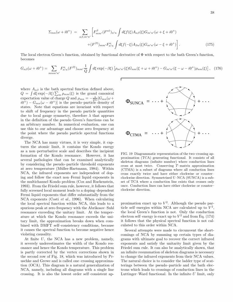
38

Σmn(ω + i0+) =∑

αβ,m′n′

[F β

mm′(Fα†)n′n

∫dξf(ξ)Aαβ(ξ)Gm′n′(ω + ξ + i0+)

+(F β†)mm′Fαn′n

∫dξf(−ξ)Aβα(ξ)Gm′n′(ω − ξ + i0+)

]. (175)

The local electron Green’s function, obtained by functional derivative of Φ with respect to the bath Green’s function,becomes

Gαβ(ω + i0+) =∑

mnm′n′

Fαn′n(F β†)mm′

1

Q

∫dξ exp(−βξ)

[ρm′n′(ξ)Gnm(ξ + ω + i0+) −Gm′n′(ξ − ω − i0+)ρnm(ξ)

], (176)

where Aαβ is the bath spectral function defined above,Q =

∫dξ exp(−βξ)∑m ρmm(ξ) is the grand canonical

expectation value of charge Q and ρmn = − 12πi [Gmn(ω+

i0+) − Gmn(ω − i0+)] is the pseudo–particle density ofstates. Note that equations are invariant with respectto shift of frequency in the pseudo particle quantitiesdue to local gauge symmetry, therefore λ that appearsin the definition of the pseudo Green’s functions can bean arbitrary number. In numerical evaluation, one canuse this to our advantage and choose zero frequency atthe point where the pseudo particle spectral functionsdiverge.

The NCA has many virtues, it is very simple, it cap-tures the atomic limit, it contains the Kondo energyas a non–perturbative scale and describes the incipientformation of the Kondo resonance. However, it hasseveral pathologies that can be examined analyticallyby considering the pseudo–particle threshold exponentsat zero temperature (Muller-Hartmann, 1984). WithinNCA, the infrared exponents are independent of dop-ing and follow the exact non–Fermi liquid exponents inthe multichannel Kondo problem (Cox and Ruckenstein,1993). From the Friedel sum rule, however, it follows thatfully screened local moment leads to a doping–dependentFermi liquid exponents that differ substantially from theNCA exponents (Costi et al., 1996). When calculatingthe local spectral function within NCA, this leads to aspurious peak at zero frequency with the Abrikosov–Suhlresonance exceeding the unitary limit. At the temper-ature at which the Kondo resonance exceeds the uni-tary limit, the approximation breaks down when com-bined with DMFT self–consistency conditions, becauseit causes the spectral function to become negative henceviolating causality.

At finite U , the NCA has a new problem, namely,it severely underestimates the width of the Kondo res-onance and hence the Kondo temperature. This problemis partly corrected by the vertex corrections shown inthe second row of Fig. 18, which was introduced by Pr-uschke and Grewe and is called one–crossing approxima-tion (OCA). This diagram is a natural generalization ofNCA, namely, including all diagrams with a single linecrossing. It is also the lowest order self–consistent ap-

ΦSUNCA = . . . + + . . .

ΦCTMA = . . . + + . . .

FIG. 19 Diagrammatic representation of the two–crossing ap-proximation (TCA) generating functional. It consists of allskeleton diagrams (infinite number) where conduction linescross at most twice. Conserving T–matrix approximation(CTMA) is a subset of diagrams where all conduction linescross exactly twice and have either clockwise or counter–clockwise direction. Symmetrized U–NCA (SUNCA) is a sub-set of TCA where a conduction line exists that crosses onlyonce. Conduction lines can have either clockwise or counter–clockwise direction.

proximation exact up to V 2. Although the pseudo par-ticle self–energies within NCA are calculated up to V 2,the local Green’s function is not. Only the conductionelectron self–energy is exact up to V 2 and from Eq. (174)it follows that the physical spectral function is not cal-culated to this order within NCA.

Several attempts were made to circumvent the short-comings of NCA by summing up certain types of dia-grams with ultimate goal to recover the correct infraredexponents and satisfy the unitarity limit given by theFriedel sum rule. It can also be analytically shown, thatan infinite resummation of skeleton diagrams is necessaryto change the infrared exponents from their NCA values.The natural choice is to consider the ladder type of scat-terings between the pseudo–particle and the bath elec-trons which leads to crossings of conduction lines in theLuttinger–Ward functional. In the infinite U limit, only

39

diagrams where all conduction electrons cross at leasttwice, are possible. Note that due to the projection, anycontribution to the Luttinger–Ward functional consistsof a single ring of pseudo–particles since at any momentin time there must be exactly one pseudo–particle in thesystem. The diagrams where all conduction electronscross exactly twice is called CTMA (Kroha et al., 1997)and has not yet been implemented in the context of theDMFT. A typical contribution to the CTMA LuttingerWard functional is shown in the second line of Fig. 19.In the impurity context, this approximation recovers cor-rect Fermi liquid infrared exponents in the whole dopingrange and it is believed to restore Fermi liquid behaviorat low temperature and low frequency.

At finite U , however, skeleton diagrams with less cross-ings exist. Namely, a ladder ring where conduction linescross exactly twice can be closed such that two conduc-tion lines cross only ones. This approximation, depictedin the first row of Fig. 19, is called SUNCA. It has beenshown in the context of single impurity calculation (Hauleet al., 2001), that this approximation further improvesthe Kondo scale bringing it to the Bethe ansatz valueand also restores Fermi liquid exponents in the strictKondo regime. Unfortunately, this is not enough to re-store Friedel sum rule in the local spectral function at lowtemperatures and to apply the approach to this regime, ithas to be combined with other approaches such as renor-malized perturbation theory or ideas in the spirit of theinterpolative methods discussed in III.F.

The results of the computationally less expensiveSUNCA calculation agree very well with the consider-ably more time consuming QMC calculation. The agree-ment is especially accurate around the most interestingregion of the Mott transition while the half–integer fillingshows some discrepancy due to the restriction to a smallnumber of valences in the SUNCA calculation.

-2 -1 0 1 2ω/D

0

0.2

0.4

QMC+MEMSUNCA

-2 0 2 4 6

ω/D

0

0.2

0.4

FIG. 20 Comparison between SUNCA (full line) and QMC(dashed line) density of states for the three–band Hubbardmodel on the Bethe lattice for nd = 0.8 at U = 5D andT = D/16.

We illustrate the agreement between these methods bymeans of the real axis data of QMC+MEM and SUNCA

where the latter results are obtained on the real axis.As shown in Fig. 20, both calculations produce almostidentical quasiparticle peak, while some discrepancy canbe observed in the shape of Hubbard bands. We believethat this is mostly due to analytic continuation of QMCdata which do not contain much high–frequency informa-tion. Notice that the width of the upper Hubbard bandis correctly obtained within SUNCA while QMC resultsshow redistribution of the weight in much broader re-gion. Namely, in the large U limit, i.e. when a bandis separated from the quasiparticle peak, its width hasto approach the width of the non–interacting density ofstates, in this case 2D.

-0.4

-0.2

0

Re G(iω) QMCIm G(iω) QMCRe G(iω) SUNCAIm G(iω) SUNCA

-0.4

-0.2

0

0 10-2

-1.5

-1

-0.5

0

ImΣ(iω) QMCImΣ(iω) SUNCA

0 10 20-2

-1.5

-1

-0.5

0

n=0.8 β=16n=0.9 β=16

n=0.8 β=16 n=0.9 β=16

FIG. 21 Imaginary axis QMC data (dots) and SUNCA results(full–lines) are compared for three–band Hubbard model onBethe lattice for β = 16 and U = 5D. Left panel shows resultsfor doping levels nd = 0.8 right panel corresponds to dopingnd = 0.9.

Finally, we compare the imaginary axis data in Fig. 21for two doping levels of nd = 0.8 and nd = 0.9. Noticethat the results are practically identical with discrepancysmaller that the error of the QMC data.

The NCA was used in the DMFT context to studyCerium (Zolfl et al., 2001), La1−xSrxTiO3 (Zolfl et al.,2000) and Ca2−xSrxRuO4 (Anisimov et al., 2002). Inthe case of Cerium, it does capture the most essentialdifferences of the alpha and gamma phases, and com-pares very favorably to the quantum Monte Carlo results(Held et al., 2001b) and to experiments. Using NCA inthe context of the SrRuO3, Anisimov et al., 2002 was thefirst to predict the so-called orbitally selective Mott tran-sition, the phase where one–band is in a Mott insultingstate while the rest are metallic. These results are dis-cussed further within (see section IV.A). The SUNCAapproach was first tested in the LaSrTiO3 where it is ina good agreement with QMC results (Oudovenko et al.,2004c).

40

C. Approaching the atomic limit: decoupling scheme,

Hubbard I and lowest order perturbation theory

The AIM Hamiltonian can also be expressed interms of Hubbard operators Xnm by replacing a†nam inEq. (170) with Xnm:

H =∑

m

EmXmm +∑

kγ

εkγc†kγckγ +

∑

k,mn,αβ

(V ∗

kαβ(Fα†)nmXnmckβ +H.c.). (177)

For convenience, we choose here the local base to be theatomic eigenbase, i.e., the atomic Hamiltonian is diago-nal.

The atomic Green’s function can be most simply de-duced from the Lehmann representation of the Green’sfunction

G(at)αβ (iω) =

1

Z

∑

nm

Fαnm(F β†)mn

(e−βEn + e−βEm

)

iω −Em +En,

(178)where F ’s are given by Fα

nm = 〈n|dα|m〉 as in sec-tion III.B and Z =

∑n e

−βEn is the partition function.The atomic Green’s function has a discrete number ofpoles, at energies corresponding to the atomic excita-tions, weighted with the appropriate factors e−βEn/Zthat can be interpreted as probabilities to find an atomin the atomic configuration |n〉.

One can compute corrections to the Green’s functionEq. (178) by expanding around the atomic limit, usingthe technique of cumulants (Metzner, 1991). Howeverthere are many resummations of these expansions, andno extensive test of this problem has been carried out.Various methods start from the equations of motion forthe Green’s functions of the Hubbard operators, for theGreen’s functions of the conduction electrons, and for themixed Green’s functions of the conduction electrons andthe Hubbard operators.

Once the Green’s functions for the Hubbard operators

Gn1n2n3n4(τ) = −〈TτXn1n2(τ)Xn3n4(0)〉, (179)

are determined, the local Green’s function Gαβ can bededuced by the following linear combination of G’s:

Gαβ(iω) =∑

n1n2n3n4

Fαn1n2

Gn1n2n3n4(iω)(F β†)n3n4 .

(180)

In the decoupling method of L. Roth (Roth, 1969), onereplaces commutator [Hhyb, X ] by a linear combinationof the operators c and X , namely

[Hhyb, Xn1n2 ] =∑

n3n4

An1n2n3n4Xn3n4 (181)

+∑

kα

Bkαn1n2

ckα +∑

kα

Ckαn1n2

c†kα,

and the coefficients A B and C are determined by pro-jecting onto the basis set of X and c, by means of a scalarproduct defined by the anticommutator. This leads to aset of closed equations for the coefficients A B and C.The Green’s function for the Hubbard operators can thenbe deduced from the following matrix equation

G−1 = G(at)−1 − ∆ − Y. (182)

where the effective hybridization function ∆ and atomicGreen’s function for the Hubbard operators G(at) are

∆n1n2n3n4 =∑

αβ

(Fα†)n1n2∆αβFβn3n4

, (183)

G(at)n1n2n3n4

(iω) =δn1n4ρn3n2 + δn2n3ρn1n4

(iω +En1 −En2), (184)

and ρ is the “density matrix”. The equations closeonce the density matrix ρ is computed from an equa-

tion such as ρn1n2 = − 1β

∑iω e

−iω0+Gn1n′n′n2(iω) or

ρn1n2 = 1β

∑iω e

iω0+Gn′n1n2n′(iω) or any combination.

The result is not unique.

Finally, the matrix Y , which is proportional to thecoefficient A introduced in Eq. (182), becomes

Yn1n2n3n4 =1

(ρn1n1 + ρn2n2)(ρn3n3 + ρn4n4)

∑

m

(Zmn2mn3δn1n4 − Zn1mn4mδn2n3), (185)

with

Zn1n2n3n4 = −T∑

n5n6

∑

iω

(∆n1n2n5n6(iω)Gn5n5n3n4(iω) + Gn3n4n5n6(iω)∆n5n6n1n2(iω)

). (186)

The equation for the Green’s function (182) is non–linear because of the coefficients X and Y , and has to

be solved iteratively. Neglecting Y results in the famous

41

Hubbard I approximation

G−1 = G(at)−1 − ∆. (187)

Perhaps, the best approximate method for the systemin the Mott–insulating state is the straightforward per-turbation expansion in hybridization strength to the low-est order. By expanding the S matrix

exp

−

∑

αβ

∫ β

0

∫ β

0

dτ1dτ2 dα(τ1)∆αβ(τ1, τ2)dβ(τ2)

,

(188)

to the lowest order, one immediately obtains the follow-ing correction to the Green’s function

Gαβ(iω) −G(at)αβ (iω) = G

(at)αβ (iω)

∑

γ,δ

∑

iω′

G(at)δγ (iω′)∆γδ(iω

′)

+

∫ β

0

dτ

∫ β

0

dτ1

∫ β

0

dτ2eiωτ∑

γ,δ

〈Tτdα(τ)d†β(0)d†γ(τ1)dδ(τ2)〉0∆γδ(τ1 − τ2). (189)

It is straightforward to evaluate the two–particleGreen’s function for the atom in Eq. (189). One can in-sert the identity |m〉〈m| between any pair of creation anddestruction operators and then integrate over time the re-sulting exponential factors. The resulting six terms, dueto six different time orderings of the product, can alsobe drawn by Feynman diagrams and evaluated by thestraightforward non–self–consistent expansion along thelines of section III.B. To make the method exact alsoin the band U = 0 limit, we calculate the lowest ordercorrection to the self–energy rather than to the Green’sfunction. The correction is

Σ = G(at)−1(G−G(at))G(at)−1 − ∆. (190)

This self–energy is exact up to second order in hybridiza-tion V and also in the non–interacting U = 0 case. Italso gives correct width of the Hubbard bands which isunderestimated by a factor of 2 by the Hubbard I approx-imation in the large U limit. This method has recentlybeen tested for the Hubbard model where it performedvery satisfactorily whenever the system has a finite gapin the one electron spectrum (Dai et al., 2005).

Many other approaches were recently used to developimpurity solvers. The local moment method (Logan andVidhyadhiraja, 2005; Vidhyadhiraja and Logan, 2004,2005) has been successfully applied to the periodic An-derson model. It would be interesting to extend it toa full multiorbital case. Also decoupling technique, ormode coupling technique, the factorization technique,the alloy analogy, the modified alloy analogy, and themethods of moments were used. These approaches canbe applied directly to the lattice and simplified usingthe DMFT locality ansatz, or applied directly to the

AIM. For a recent review with a DMFT perspective see(Shvaika, 2000).

D. Quantum Monte Carlo: Hirsch–Fye method

The general idea underlying the Hirsch–Fye deter-minantal QMC method is to discretize the path inte-grals representing the partition function and the Green’sfunction of an interacting problem. These discretizedpath integrals are then converted, using a Hubbard–Stratonovich transformation, into a statistical averageover a set of non–interacting Green’s functions in a time–dependent field, which can be either continuous or dis-crete. The sum over the auxiliary fields is done usingMonte Carlo sampling methods. The QMC algorithm forthe solution of the Anderson impurity model was intro-duced in (Fye and Hirsch, 1989; Hirsch and Fye, 1986),and generalized to the multiorbital case in (Takegahara,1993) and (Bonca and Gubernatis, 1993). Applicationsto the solution of the lattice models via DMFT was intro-duced in (Jarrell, 1992), see also (Georges and Krauth,1992; Jarrell and Akhlaghpour, 1993; Rozenberg et al.,1992) in the single–orbital case. In the multiorbital con-text it was implemented in (Rozenberg, 1997), see also(Held and Vollhardt, 1998). Some DMFT applications,such as the study of the electron–phonon interactionswithin single–site DMFT, require a QMC implementa-tion using continuous Hubbard–Stratonovich fields (Jar-rell and Akhlaghpour, 1993). This is also essentialfor the implementation of Extended Dynamical Mean–Field Theory (EDMFT) (see for example (Motome andKotliar, 2000), (Pankov et al., 2002) and for the combi-

42

nation of EDMFT and GW method (Sun and Kotliar,2002)). An alternative algorithm for EDMFT using dis-crete spins was introduced in (Grempel and Rozenberg,1998). Zero temperature QMC algorithms, which areclosely related to determinantal algorithms, have beenextensively developed for lattice models. DMFT applica-tions have been recently introduced in (Feldbacher et al.,2004). There are alternative methods of evaluating thepartition function and the correlation functions, whichare amenable to Monte Carlo methods (Rombouts et al.,1999). These are free of discretization errors and havebeen introduced in (Rubtsov, 2003; Rubtsov et al., 2004;Savkin et al., 2005) in the DMFT context.

QMC has been used extensively in DMFT calcula-tions. Due to space limitations, only a few illustra-tive examples shall be described. The QMC methodhas been applied to the study of Cerium by McMahanand collaborators (Held et al., 2001b; McMahan et al.,2003) and to Iron and Nickel by Lichtenstein and col-laborators (Katsnelson and Lichtenstein, 2000; Lichten-stein et al., 2001). DMFT with QMC as an impuritysolver, has been applied to many other d–electron sys-tems. These include perovskites with a d1 configura-tion such as LaTiO3 (Nekrasov et al., 2000) SrVO3 andCaVO3 (Pavarini et al., 2004; Sekiyama et al., 2004),ruthenates such as RuSrO4 (Liebsch, 2003a; Liebsch andLichtenstein, 2000b) and vanadates such as V2O3 (Heldet al., 2001a) and VO2 (Biermann et al., 2005b).

Since a detailed review (Georges et al., 1996) for thesingle–orbital case is already available, we focus hereon the generalization of the QMC method for multior-bital or cluster problems (for the impurity solver, “clus-ter DMFT” is a particular case of multiorbital DMFTwhere the cluster index plays the role of an orbital). Theemphasis of this section is on generality; for a more ped-agogical introduction to the method in a simple case, see(Georges et al., 1996). This section is organized as fol-lows. First in III.D.1, we present the general impurityproblem to be solved by QMC. In III.D.2 we presentthe Hirsch–Fye algorithm, where we discuss the timediscretization, derive the discrete Dyson equation, andpresent the algorithm. In III.D.2.e, we present in moredetail the case of density–density interactions, which hasbeen the most widely used. Details of the derivations areprovided in Appendix A for completeness.

1. A generic quantum impurity problem

a. Definitions We will focus on the solution of a genericquantum impurity problem like (85) defined by the fol-

lowing action

Seff = −∫∫ β

0

dτdτ ′∑

1≤µ,ν≤N1≤σ≤Nσ

d†µσ(τ)G−10σµν (τ, τ ′)dνσ(τ ′)

+

∫ β

0

dτHint(τ) (191a)

Hint ≡Uσ1σ2σ3σ4µ1µ2µ3µ4

d†µ1σ1dµ2σ2d

†µ3σ3

dµ4σ4 (191b)

where G−10σµν is the Weiss function, 1 ≤ σ ≤ Nσ are in-

dices in which the Green’s functions are diagonal (con-served quantum numbers), 1 ≤ µ, ν ≤ N are indices inwhich the Green’s functions are not diagonal, and re-peated indices are summed over. The value of N and Nσ

depends on the problem (see III.D.1.c). Hint is the inter-action part of the action. It should be noted that we havedefined a completely general Hint, which is necessary tocapture multiplets which occur in real materials. Thepurpose of the impurity solver is to compute the Green’sfunction

Gσµν (τ) =⟨Tdµσ(τ)d†νσ(0)

⟩Seff

(192)

and higher order correlation functions. In this section, we

will use a different convention for the sign of the Green’s

function than in the rest of this review: in accordancewith (Georges et al., 1996) and the QMC literature, wedefine the Green’s functions without the minus sign.

b. Generalized Hubbard–Stratonovich decoupling Hirsch–Fye QMC can only solve impurity problems where theinteraction have a decoupling formula of the followingform

Hint = H1 + · · · +Hn (193a)

e−∆τHi =∑

Si∈Si

wi(Si) exp

(∑

σµν

d†µσViσµν (Si)dνσ

)

(193b)

where Si is a index (referred to in the following asa “QMC–spin”) in a set Si (discrete or continuous),

wi(Si) > 0 is a positive weight, V = V †, and Hi = H†i .

Approximate decouplings, where (193) holds only up toO(∆τm),m ≥ 3, are discussed below (see also (Gunnars-son and Koch, 1997)). Equation (193a) is a generalizedform of the familiar Hubbard–Stratonovich transforma-tion. Multiple Hubbard–Stratonovich fields per time sliceallow the decoupling of more general interactions, as ex-emplified below.

c. Examples Let us consider first a multiorbital or clus-ter DMFT solution of the Hubbard model in the nor-mal phase (non–superconducting). In this case, N is thenumber of impurity sites or orbitals, and Nσ = 2: σ is

43

the spin index which is conserved. The interaction termHint is given by

Hint =∑

(µ,σ)<(ν,σ′)

Uσσ′

µν nσµn

σ′

ν (194)

where we use the lexicographic order: (µ, σ) < (ν, σ′) ifµ < ν or µ = ν and σ < σ′. In this case, the decouplingformula uses the discrete Hubbard–Stratonovich trans-formation using Ising spins introduced by Hirsch (Hirsch,1983) (see also (Takegahara, 1993) and (Bonca and Gu-bernatis, 1993))

e−∆τHint =1

2

∑

Sσσ′µν =±1

exp

[ ∑

(µ,σ)<(ν,σ′)

(λσσ′

µν Sσσ′

µν (nσµ − nσ′

ν ) − ∆τUσσ′

µν

2(nσ

µ + nσ′

ν )

)]

(195)

λσσ′

µν ≡ arccosh

(exp

(∆τ

2Uσσ′

µν

))(196)

The weight w(S) = 12 is independent of the auxiliary

Ising fields Sσσ′

µν defined for each U term. The matrix Vof Eq. (193) is diagonal and reads

V σµν(S) =δµν

∑

ρ,σ′

(µ,σ)<(ρ,σ′ )

(λσσ′

µρ Sσσ′

µρ − ∆τ

2Uσσ′

µρ )−

δµν

∑

ρ,σ′

(µ,σ)>(ρ,σ′ )

(λσ′σρµ Sσ′σ

ρµ +∆τ

2Uσ′σ

ρµ ) (197)

A general goal of the Hirsch–Fye algorithm is to minimizethe number of decoupling fields, to reduce the size of theconfiguration space where the Monte Carlo is done (seebelow). In this respect, decoupling each U term in theinteraction with a different field is not optimal, especiallywhen there is a symmetry between orbitals. However,there is currently no efficient solution to this problem.

A second example is the study of a superconductingphase. We restrict our discussion to the Hubbard modelfor simplicity, but the generalization to more realisticmodels is straightforward. For the study of supercon-ductivity in a two–band model see (Georges et al., 1993).For the QMC calculation of d–wave superconductivity ina cluster see (Lichtenstein and Katsnelson, 2000; Maieret al., 2000b). We restrict ourselves to a case where apossible antiferromagnetic order and the superconduct-ing order are collinear. In this case, we introduce the

Nambu spinor notation at each site i: ψ† ≡ (d†↑, d↓) sothat the Green’s function is

G(τ) ≡⟨Tτψ(τ)ψ†(0)

⟩=

(G↑(τ) F (τ)

F ∗(τ) G↓(β − τ)

)(198)

where F is the anomalous Green’s function F (τ) =〈Tτd↑(τ)d↓(0)〉. We denote by + and − the Nambu in-dices, and n+ = n↑ and n− = 1−n↓. In this case, we take

Nσ = 1 (spin is not conserved) and N = 2Nnormal case,twice the number of sites. The index µ is a double index(i,±), where i is a site index. For simplicity, we take alocal U interaction, which is then decoupled as (for eachcluster site)

exp

(−∆τUni↑ni↓

)∝

∑

Si=±λ

e−Si

2eSi(ni++ni−)−∆τU

2 (ni+−ni−)

with λ = arccosh(exp(∆τU/2

)(we drop a constant since

it cancels in the algorithm).A third example is a further generalization of the

Hirsch–Fye formula to decouple the square of some op-erator. For example, if M has a spectrum contained in0,±1,±2, one can use

eαM2

=∑

σ=0,±S

wσeσM (199a)

S = cosh−1

(e3α + e2α + eα − 1

2

)(199b)

wS = w−S =eα − 1

e3α + e2α + eα − 3(199c)

w0 = 1 − 2wS (199d)

This can be used to decouple a nearest neighbor density–density interaction in a Hubbard model (as an alterna-tive to the more commonly used method that splits thisinteraction into four terms using n = n↑ + n↓ and theHirsch–Fye formula).

In the case of a quantum impurity problem formu-lated in a general non–orthogonal basis, we can orthog-onalize within the impurity degree of freedom (how-ever, there may still be an overlap between different unitcells), in order to reduce the problem to the case wherethe c basis is orthogonal. The V matrix transforms asV ′ = (P †)−1V P−1, where P is the matrix that trans-form into the orthogonal basis. Note however that ingeneral a diagonal V will transform into a non–diagonalV ′, which will make the QMC more costly.

2. Hirsch–Fye algorithm

a. Time discretization We start by writing a Hamiltonianform H = H0 + Hint of the action using an effectivegeneralized Anderson model with ns bath sites

H0 =

ns∑

p=1

∑

µνσ

ε0pσµνa†pµσapνσ +

∑

pµνσ

V 0pµνσ(a†pνσdµσ + h.c.)

+ εµνσd†µσdνσ

(200)

Kσpµ,p′ν is defined as follows

Hσ0 ≡

∑

pµp′ν

a†pµσKσpµ,p′νap′νσ (201)

44

where H0 ≡∑σ Hσ0 , and apµσ is the annihilation opera-

tor of the electron on the bath site for p > 0 and for p = 0we identify d = ap=0 which corresponds to the impuritysite. In the Hirsch–Fye algorithm, the imaginary time is

discretized with L discrete times τl = (l − 1)β/L, with1 ≤ l ≤ L. Using the Trotter formula, we approximatethe partition function by Z ≈ Z∆τ with

Z∆τ ≡Tr

L∏

l=1

(exp−∆τH0

n∏

i=1

exp−∆τHi

)(202)

Z∆τ =∑

Sli

(L∏

l=1

n∏

i=1

wi(Sli)

)∏

σ

Tr

L∏

l=1

[e−∆τH0

n∏

i=1

exp

(∑

µν

d†µσViσµν (Sl

i)dνσ

)](203)

where Sli are L copies of the decoupling QMC–spins. The

Green’s function defined in (192) at time τl

Gσ;µν(τl1 , τl2) =1

ZTr(UL−l1dµσU

l1−l2d†νσUl2)

(204a)

U ≡ e−∆τH (204b)

for 1 ≤ µ, ν ≤ N and l1 ≥ l2, is replaced by its discretizedversion

G∆τσ;(l1,µ),(l2,ν) ≡

1

Z∆τTr(U

L−l1+1dµσU

l1−l2d†νσU

l2−1)

(205a)

U ≡∏

0≤i≤n

∑

Si∈Si

wi(Si) exp

(d†ρσV

iσρλ (Si)dλσ

)

U =∏

0≤i≤n

e−∆τHi +O(∆τm) (205b)

Since the Trotter formula is an approximation con-trolled by ∆τ , one may use approximate decoupling for-mulas, up to order O(∆τm) (m ≥ 3), that would not in-troduce a priori a bigger error than the Trotter formulaitself. For density–density interactions exact formula areavailable (as described above) but for a more general

interactions this may not be the case. A priori, U =U+O(∆τ2) thus G∆τ = G+O(∆τ) (since L×O(∆τ 2) =O(∆τ)). However, given that H is hermitian, we see that

G is hermitian Gσ;µν(τl1 , τl2) =(Gσ;νµ(τl1 , τl2)

)∗. Using

U = U(1 − (∆τ)2/2

∑i<j [Hi, Hj ] + O(∆τ3)

), the fact

that the commutator is anti–hermitian when all the Hi

are hermitian, and U † = U , we get Z∆τ = Z + O(∆τ2)and the stronger result

Gσ;µν(τl1 , τl2) =G∆τ

σ;(l1,µ),(l2,ν) +(G∆τ

σ;(l1,ν),(l2,µ)

)∗

2+O(∆τ2)

(206)

Eq. (206) shows that i) we gain one order in ∆τ withsymmetrization, ii) various hermitian Hi can be decou-pled separately to the same order, and iii) we only needa decoupling formula that is correct up to order (∆τ 2)included.

b. The Dyson equation Let us introduce a matrix of sizeNns defined by

V iσ(S)|pµ,p′ν ≡ δpp′δp0Viσµν (S) (207)

and the notation S ≡ Sli, 1 ≤ i ≤ n; 1 ≤ l ≤ L for

a configuration of the QMC–spin, we have immediatelyfrom (202)

Z∆τ =∑

S

(L∏

l=1

n∏

i=1

wi(Sli)

)Z[S] (208)

Z[S] ≡∏

σ

[Tr

1∏

l=L

(exp

(−∆τa†pµσKσ

pµ,p′νap′νσ

)×

n∏

i=1

exp

(a†pµσV iσ(Sl

i)|pµ,p′νap′νσ

))](209)

Introducing, Nns ×Nns matrices Bl(S) defined by

Bl(S) ≡ exp

(−∆τKσ

) n∏

i=1

exp

(V iσ(S)

)(210)

we can rewrite the partition function as (see Ap-pendix A):

Z[S] =∏

σ

detOσ(S) (211a)

Oσ(S) ≡

1... 0 Bσ

L(SLi )

−Bσ1 (S1

i )... . . . 0

0... . . . . . .

. . .... 1 0

. . .... −Bσ

L−1(SL−1i ) 1

(211b)

Note that Oσ has size LNns. Moreover, the Green’sfunction for a fixed QMC–spins configuration, defined asin Eq. (205a) can be shown to be (see A)

gσS = O−1

σ (S) (212)

45

The formula for the partition function can be generalizedto the average of any operator M

〈M〉 =

∑S 〈M〉S

(∏i,l wi(S

li))∏

σ detOσ(S)∑

S

(∏i,l wi(Sl

i))∏

σ detOσ(S)(213)

where 〈M〉S is the average of the operator at fixed con-

figuration S. In particular, the Green’s function isgiven by averaging gσ

S. Moreover, for a fixed QMC–

spins configuration, the action is Gaussian, allowing tocompute any correlation functions with Wick theorem.As noted in (Hirsch and Fye, 1986) (see also (Georgeset al., 1996), one can derive a simple Dyson relation be-tween the Green’s functions of two configurations gS andgS′

gσS′ = gσ

S + (gσS − 1)×

( 1∏

i=n

e−eViσ(S)

n∏

i=1

eeViσ(S′) − 1

)gσS′ (214)

with the notation

V iσpµl,p′νl′(S) = δl,l′V iσ

pµ,p′ν(Sli) (215)

(see Appendix A). Since V acts non–trivially only on thep = 0 subspace, we can project (214) on it and get ridof the auxiliary variables. We obtain finally the Dysonequation for the Green’s function G (defined as in (205)and considered here as a matrix of size LN )

GS′σ = GS

σ + (GSσ − 1)×

( 1∏

i=n

e−eV iσ(S)

n∏

i=1

eeV iσ(S′) − 1

)GS′

σ (216)

where

V iσµl,νl′ (S) = δl,l′V

iσµ,ν(Sl

i) (217)

We used the fact that G and V are diagonal in the σindex. Eq. (216) is a equation for matrices of size NL.

We note that (216) also holds for a special caseV (S) = 0, with GS = G0. This gives a simple way tocompute GS from G0, which requires the inversion of aLN × LN matrix Aσ .

GSσ = A−1

σ G0σ (218a)

Aσ ≡ 1 +(1 − G0σ

)( n∏

i=1

eeV iσ(S) − 1

)(218b)

Eq. (218) is often referred to as the “full update for-mula”.

Moreover, there is an important simplified relation be-tween two close configurations S and S ′ which differ

only for one QMC–spin Sli , which allows a faster update

of the Green’s function in the algorithm

GS′σ = A−1

σ GSσ (219)

Aσ ≡ 1 +(1 −GS

σ

)( i∏

j=n

e−eV jσ(S)

n∏

j=i

eeV jσ(S′) − 1

)

can be reduced to

p ≡∏

σ

detOσ(S′)

detOσ(S)=∏

σ

detAσ =∏

σ

detAσll

(220a)

Aσll ≡ 1 +

(1 −G

Sσ;ll

)Cσ

ll (220b)

Cσll ≡

i∏

j=n

e−V jσ(Slj)

n∏

j=i

eV jσ(S′lj ) − 1 (220c)

GS′σ;l1l2

= GSσ;l1l2

+(G

Sσ;l1l − δl1l

)Cσ

ll(Aσll)

−1GSσ;ll2

(220d)

Eq. (220) is often referred to as the “fast update for-mula” (Hirsch, 1983). It is a formula for matrices of sizeN (compared to LN for the full update). It does notinvolve a big matrix inversion, therefore it allows a fastercalculation of G than (218). For density–density inter-actions, the fast update formula can be further simpli-fied (with no matrix inversion, see below). These equa-tions are the generalizations of Eqs. (130)1 and (131) of(Georges et al., 1996).

c. The Hirsch–Fye algorithm In principle, the sum (213)could be done by exact enumeration (Georges andKrauth, 1993), (Georges et al., 1996) but in practice onecan reach much lower temperatures by using statisticalMonte Carlo sampling. It consists of the generation ofa sample of QMC–spins configuration S with proba-bility

∏i,l wi(S

li)∏

σ detOσ(S). If the determinant isnot positive, one needs to take the absolute value of thedeterminant to define the probabilities and sample thesign. After computing GS from G0 with the “full up-date” formula (218), a Markov chain is constructed bymaking local moves, one time slice at a time, selecting anew value for one QMC–spin and using the “fast update”formula (220) to compute the Green’s function for thenew QMC–spin configuration. It may also be convenientto perform global moves that involve the simultaneousflipping of many spins in one move (e.g. simultaneousflipping of all the spins in all the time slices). This canbe accomplished directly using (218) or by generatingthe global move as a sequence of local moves with (220)(one has then to keep and restore the Green’s function to

1 Eq. (130) in (Georges et al., 1996) has a misprint and should be

read as G′

l1l2= Gl1l2 + (G− 1)l1l(e

V ′−V

− 1)ll(All)−1Gll2 .

46

the original configuration in the case that the proposedglobal move is rejected). An interesting generalization ofthis global move was proposed by Grempel and Rozen-berg (Grempel and Rozenberg, 1998), in which one up-dates different Fourier components of the fields. As notedabove, the computation allows, in practice, the compu-tation of any higher order correlation function since thetheory is Gaussian for a fixed QMC–spin configuration.

It should be noted that for some cases of cluster or mul-tiorbital problems, this QMC algorithm suffers severelyfrom the sign problem at low temperature, particularly inthe case of frustrated systems (Parcollet et al., 2004). Inthe single–site DMFT case, this problem is absent: thishad been known empirically for a while and rigorouslyproved recently (Yoo et al., 2004).

d. Remarks on the time discretization There is three diffi-culties coming from the discretization of the time in theHirsch-Fye algorithm:

i) One has to take a large enough number of time slicesL, or in practice to check that the results are unchangedwhen L is increased, which is costly since the computa-tion time increase approximately like L3.

ii) Since the number of time slices is limited, espe-cially for multi–orbital or cluster calculation, the eval-uation of the Fourier transform of the Green’s function(Matsubara frequencies) is delicate. In practice, the timeGreen’s function is constructed from the discrete func-tion resulting from the QMC calculation using splines,whose Fourier transform can be computed analytically(see (Georges et al., 1996)). It turns out however that forthis technique to be precise, one needs to supplement thediscrete Green’s function by the value of its derivatives atτ = 0, β, which can be reduced to a linear combination oftwo–particle correlation functions computed by the QMCcalculation (Oudovenko and Kotliar, 2002). Failure todeal with this problem accurately can lead in some cal-culations to huge errors, which can manifest themselvesby spurious causality violations.

iii) When a computation is made far from the particle-hole symmetric case, the Weiss function G0 can be verysteep close to τ = 0 or τ = β. As a result, it isnot well sampled by the regular mesh time discretiza-tion, leading to potentially large numerical error. A sim-

ple practical solution is to replace G0 by G−10 (iωn) ≡

G−10 (iωn) − α where α is a diagonal matrix chosen asαµµ = limω→∞(G−1

0 )µµ(ω). From Eqs. (191a), we seethat the new impurity problem which is equivalent ifthe α term (which is quadratic in d and diagonal in theindices) is simultaneously added to the interaction (orequivalently to the right hand side of the correspondingdecoupling formula). In the new impurity problem how-ever G0 is less steep than G0 close to τ = 0 or τ = β, sothe numerical error introduced by discretization is lessimportant.

e. Density–density interactions The “fast update” for-mula can be further simplified when the matrix V isdiagonal, particularly in the case of density–density in-teractions, which is used in most of the calculations withthe Hirsch–Fye algorithm. To be specific, we concentratein this paragraph on the first example given above (thenormal state of a Hubbard model). The matrix V of Eq.(193) is diagonal and given by (197). The “fast update”

formula (220) for the flip of the Ising spin Slσσ′

µν at thetime slice τl simplifies. The non–zero elements of thematrix C are given by

C σll;µµ = exp

(2λσσ′

µν S′σσ′

µν

)− 1 (221a)

C σ′

ll;ν ν = exp(−2λσσ′

µν S′σσ′

µν

)− 1 (221b)

Let us first consider the case σ = σ′. p reduces to

p = ξµξν −GSσ;(l,µ);(l,ν)G

Sσ;(l,ν);(l,µ)C

σll;µµC

σll;ν ν (222)

ξρ ≡(

1 +(1 −G

Sσ;(l,ρ);(l,ρ)

)C σ

ll;ρρ

); ρ = µ, ν (223)

Defining M by

M11 = ξνCσll;µµ/p (224a)

M22 = ξµCσll;ν ν/p (224b)

M12 = GSσ;(l,µ),(l,ν)C

σll;µµC

σll;ν ν/p (224c)

M21 = GSσ;(l,ν),(l,µ)C

σll;µµC

σll;ν ν/p (224d)

we have the “fast update” formula

GS′σ;(l1,µ),(l2,ν) = G

Sσ;(l1,µ),(l2,ν) + δσσ

[(G

Sσ;(l1,µ),(l,µ) − δ(l1,µ),(l,µ)

)(M11G

Sσ;(l,µ),(l2,ν) +M12G

Sσ;(l,ν),(l2,ν)

)+

(G

Sσ;(l1,µ),(l,ν) − δ(l1,µ),(l,ν)

)(M21G

Sσ;(l,µ),(l2,ν) +M22G

Sσ;(l,ν),(l2,ν)

)]

This equation can also be obtained by using the fast up-date (Sherman–Morrison) formula twice.

The case where σ 6= σ′ is more straightforward

p =ξξ′ (225a)

ξ ≡(

1 +(1 −G

Sσ;(l,µ);(l,µ)

)C σ

ll;µµ

)(225b)

ξ′ ≡(

1 +(1 −G

Sσ′;(l,ν);(l,ν)

)C σ′

ll;νν

)(225c)

47

GS′σ;(l1,µ),(l2,ν) = G

Sσ;(l1,µ),(l2,ν)+

δσσCσll;µµG

Sσ;(l,µ),(l2,ν)

(G

Sσ;(l1,µ),(l,µ) − δ(l1,µ),(l,µ)

)/ξ+

δσσ′C σ′

ll;ννGSσ;(l,ν),(l2,ν)

(G

Sσ;(l1,µ),(l,ν) − δ(l1,µ),(l,ν)

)/ξ′

(226)

f. Analytic continuation The quantum Monte Carlo sim-ulation yields the Green’s function in imaginary timeG(τ). For the study of the spectral properties, transportor optics, Green’s function on real axis are needed andtherefore the analytic continuation is necessary. This inpractice amounts to solving the following integral equa-tion

G(τ) =

∫dωf(−ω)e−τωA(ω) (227)

where A(ω) is the unknown spectral function, and f(ω)is the Fermi function. This is a numerically ill-posedproblem because G(τ) is insensitive to the spectral den-sity at large frequencies. In other words, the inverse ofthe kernel K(τ, ω) = f(−ω)e−τω is singular and somesort of regularization is necessary to invert the kernel.Most often, this is done by the maximum entropy method(MEM) (Jarrell and Gubernatis, 1996).

A new functional Q[A], which is to be minimized, isconstructed as follows

Q[A] = αS[A] − 1

2χ2[A] (228)

where χ2

χ2[A] =

L∑

ij=1

(Gi −G(τi))[C−1]ij(Gj −G(τj)) (229)

measures the distance between the QMC data, averagedover many QMC runs (Gi) and the Green’s functionG(τi) that corresponds to the given spectral functionA(ω) according to equation Eq. (227). Cij is the co-variant matrix that needs to be extracted from the QMCdata when measurements are not stochastically indepen-dent. The entropy term, S[A], takes the form

S[A] =

∫(A(ω) −m(ω) −A(ω) ln [A(ω)/m(ω)]) ,

(230)where m(ω) is the so-called default model, usually cho-sen to be a constant, or, alternatively, taken to be thesolution of the same model but calculated by one of theavailable approximations.

For each value of the parameter α, numeric minimiza-tion of Q gives as the corresponding spectral functionAα(ω). If α is a large number, the solution will not movefar from the default model, while small α leads to unphys-ical oscillations caused by over-fitting the noisy QMCdata. In the so-called historic MEM, the parameter α is

chosen such that χ2 = N , where N is the total number ofreal frequency points at which A(ω) is being determined.In many cases, this gives already a reasonable spectralfunctions, however, in general the historic method tendsto underfit the data and makes the resulting A(ω) toosmooth.

In the classical MEM, the parameter α is determinedfrom the following algebraic equation

−2αS(α) = TrΛ(α) [αI + Λ(α)]−1

(231)

where S(α) is the value of the entropy in the solution Aα,which minimizes Q and Λ(α) is

Λ(α)ij =√Aα

i

[KTC−1K

]ij

√Aα

j . (232)

Here Kij is the discretized kernel Kij ≡ K(τi, ωj) andAi is the discretized spectral function Ai = A(ωi)dωi

and Cij is the above defined covariant matrix.In applications of DMFT to real materials, the quasi-

particle peak can have a complex structure since at lowtemperature it tries to reproduce the LDA bands aroundthe Fermi-level, i.e., the spectral function approaches theLDA density of states contracted for the quasiparticlerenormalization amplitude Z, A(ω) = ρ(ω/Z + µ0). TheMEM method has a tendency to smear out this complexstructure because of the entropy term. At low tempera-ture, this can lead to the causality violation of the impu-rity self-energy. To avoid this pathology, it is sometimesuseful to directly decompose the singular kernel with theSingular Value Decomposition (SVD). When construct-ing the real frequency data, one needs to take into ac-count only those singular values, which are larger thanprecision of the QMC data.

The discretized imaginary time Green’s function G(τi)can be SVD decomposed in the following way

G(τi) =∑

j

KijAj =∑

jm

VimSmUmjAj (233)

where UU † = 1 and V †V = 1 are orthogonal matricesand S is diagonal matrix of singular values. The inversionis then

Aj =∑

m<M,i

Umj1

SmVimGi (234)

where the sum runs only up to M determined by theprecision of the QMC data, for example SM > 〈ViM δGi〉,where δGi is the error estimate for Gi. The magnitudeof the singular values drop very rapidly and only of order10 can be kept.

The SVD does not guarantee the spectra to be pos-itive at higher frequencies nor does it give a renormal-ized spectral function. This however does not preventus from accurately determining those physical quantitieswhich depend on the low frequency part of spectra as forexample transport or low frequency photoemission.

48

E. Mean–field slave boson approach

In this section we describe a different slave boson rep-resentation, which allows a construction of a mean–fieldtheory closely related to the Gutzwiller approximation.In this method we assign a slave boson ψm to each atomicstate |m〉 and slave fermion fα to each bath channel suchthat the creation operator of an electron is given by

d†α = z†αf†α, (235)

with

z†α =∑

m,n

ψ†n(Fα†)nmψm ≡ ψ†Fα†ψ. (236)

The matrix elements Fαnm are closely related to those in

Eq. (169) with an important difference: here one repre-sents electron operator by a product of pseudo–fermionand two pseudo–bosons. The fermionic presign is com-pletely taken care of by the pseudo fermion, and there-fore the matrix elements that appear in the definition ofpseudo–bosons should be free of the fermionic presign.In other words, when calculating matrix F in the directbase, where matrix elements are either 0, +1 or −1, oneshould take absolute values. In the direct base, the defi-

nition of Fα is then

Fαnm = |〈n|dα|m〉|. (237)

The enlarged Hilbert space contains unphysical statesthat must be eliminated by imposing the set of con-straints

Q ≡ ψ†ψ = 1 (238)

f †αfα = ψ†Fα†Fαψ. (239)

The first constraint merely expresses the completenessrelation of local states, while the second imposes equiv-alence between the charge of electrons on the local leveland charge of pseudo–fermions.

Introduction of these type of Bose fields allows one tolinearize interaction term of type Uαβnαnβ. For moregeneral type of interaction, one needs to introduce addi-tional bosonic degrees of freedom that are tensors in thelocal Hilbert space instead of vectors. Additional con-straints then can diagonalize a more general interactionterm.

Following Ref. (Kotliar and Ruckenstein, 1986) ad-ditional normalization operators Lα and Rα are intro-duced whose eigenvalues would be unity if the constraintsEq. (238) are satisfied exactly but at the same time guar-antee the conservation of probability in the the mean–field type theory

Rα = (1 − ψ†FαFα†ψ)−1/2, (240)

Lα = (1 − ψ†Fα†Fαψ)−1/2. (241)

With this modification, the creation operator of an elec-tron is still expressed by d†α = z†αf

†α with projectors equal

to

z†α = Rα ψ†Fα†ψ Lα. (242)

The action of the AIM may now be written in termsof pseudo particles as

S =∑

α

∫ β

0

dτ

[f †

α(∂

∂τ− µ+ iλα)fα + ψ†(−iλαF

α†Fα)ψ

]+

∫ β

0

dτ ψ†(∂

∂τ+ iΛ +E)ψ (243)

+∑

α,β

∫ β

0

dτ

∫ β

0

dτ ′ z†α(τ)f †α(τ)∆αβ(τ − τ ′)fβ(τ ′)zβ(τ ′) − iΛ, (244)

where iΛ and iλα are introduced for the constraintsEq. (238) and (239), respectively.

After integrating out pseudo fermions, the following

saddle–point equations can be derived by minimizing freeenergy with respect to classical fields ψ

1

β

∑

iω

∑

α,β

[1

2(Ggαβz

†β∆βαzα + z†α∆αβzβGgβα)(L2

αFα†Fα +R2

αFαFα†)

+LαRα(Ggαβz†β∆βαF

α + ∆αβzβGgβαFα†)]ψ + (iΛ +E −

∑

α

iλαFα†Fα)ψ = 0. (245)

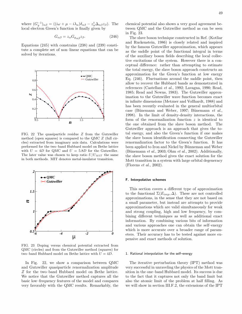
49

where (G−1g )αβ = ((iω + µ − iλα)δαβ − z†α∆αβzβ). The

local electron Green’s function is finally given by

Gαβ = zαGgαβzβ. (246)

Equations (245) with constrains (238) and (239) consti-tute a complete set of non–linear equations that can besolved by iterations.

0.5 1 1.5 2n

0

0.2

0.4

0.6

0.8

1

Z

QMCGutzwiller

FIG. 22 The quasiparticle residue Z from the Gutzwillermethod (open squares) is compared to the QMC Z (full cir-cles) extracted from imaginary axis data. Calculations wereperformed for the two–band Hubbard model on Bethe latticewith U = 4D for QMC and U = 5.8D for the Gutzwiller.The later value was chosen to keep ratio U/UMIT the samein both methods. MIT denotes metal-insulator transition.

-6 -4 -2 0µ

0.5

1

1.5

2

n

QMCGutzwiller

FIG. 23 Doping versus chemical potential extracted fromQMC (circles) and from the Gutzwiller method (squares) fortwo–band Hubbard model on Bethe lattice with U = 4D.

In Fig. 22, we show a comparison between QMCand Gutzwiller quasiparticle renormalization amplitudeZ for the two–band Hubbard model on Bethe lattice.We notice that the Gutzwiller method captures all thebasic low–frequency features of the model and comparesvery favorably with the QMC results. Remarkably, the

chemical potential also shows a very good agreement be-tween QMC and the Gutzwiller method as can be seenin Fig. 23.

The slave boson technique constructed in Ref. (Kotliarand Ruckenstein, 1986) is closely related and inspiredby the famous Gutzwiller approximation, which appearsas the saddle point of the functional integral in termsof the auxiliary boson fields describing the local collec-tive excitations of the system. However there is a con-ceptual difference: rather than attempting to estimatethe total energy, the slave boson approach constructs anapproximation for the Green’s function at low energyEq. (246). Fluctuations around the saddle point, thenallow to recover the Hubbard bands as demonstrated inreferences (Castellani et al., 1992; Lavagna, 1990; Read,1985; Read and Newns, 1983). The Gutzwiller approx-imation to the Gutzwiller wave function becomes exactin infinite dimensions (Metzner and Vollhardt, 1988) andhas been recently evaluated in the general multiorbitalcase (Bunemann and Weber, 1997; Bunemann et al.,1998). In the limit of density-density interactions, theform of the renormalization function z is identical tothe one obtained from the slave boson method. TheGutzwiller approach is an approach that gives the to-tal energy, and also the Green’s function if one makesthe slave boson identification connecting the Gutzwillerrenormalization factor to the Green’s function. It hasbeen applied to Iron and Nickel by Bunneman and Weber(Bunemann et al., 2003; Ohm et al., 2002). Additionally,the slave boson method gives the exact solution for theMott transition in a system with large orbital degeneracy(Florens et al., 2002).

F. Interpolative schemes

This section covers a different type of approximationto the functional Σ(Eimp,∆). These are not controlledapproximations, in the sense that they are not based ona small parameter, but instead are attempts to provideapproximations which are valid simultaneously for weakand strong coupling, high and low frequency, by com-bining different techniques as well as additional exactinformation. By combining various bits of informationand various approaches one can obtain the self–energywhich is more accurate over a broader range of param-eters. Their accuracy has to be tested against more ex-pensive and exact methods of solution.

1. Rational interpolation for the self–energy

The iterative perturbation theory (IPT) method wasvery successful in unraveling the physics of the Mott tran-sition in the one–band Hubbard model. Its success is dueto the fact that it captures not only the band limit butalso the atomic limit of the problem at half filling. Aswe will show in section III.F.2, the extensions of the IPT

50

method are possible, but less reliable in the multiorbitalcase. There have been some attempts to “define” inter-polative methods that are robust enough and give rea-sonable results in the whole space of parameters of anmultiorbital impurity model.

In this section, we will review the ideas from (Savrasovet al., 2004) where a simple rational form for the self–energy was proposed and unknown coefficient from thatrational expression were determined using the slave bo-son mean–field (SBMF) method. This scheme tries toimprove upon SBMF, which gives the low–frequency in-formation of the problem, by adding Hubbard bands tothe solution. For simplicity, only SU(N) symmetry willbe considered.

It is clear that Hubbard bands are damped atomic ex-citations and to the lowest order approximation, appearat the position of the poles of the atomic Green’s func-tion. Therefore, a good starting point to formulate thefunctional form for the self–energy might be the atomicself–energy

Σ(at)(iω) = iω − εf −[G(at)(iω)

]−1

, (247)

where

Gat(iω) =N−1∑

n=0

CN−1n (Pn + Pn+1)

iω + µ−En+1 +En, (248)

and En = εfn + 12Un(n − 1), Pn is the probability to

find an atom in a configuration with n electrons, and

CN−1n = (N−1)!

n!(N−n−1)! arises due to the equivalence of all

states with n electrons in SU(N).The atomic self–energy can also be brought into the

form

Σ(at)(iω) = iω − εf −

N∏i=1

(iω − Zi)

N−1∏i=1

(iω − Pi)

, (249)

where Zi are zeros and Pi are the N −1 poles, which canbe calculated from equations (247) and (248). Using thesame functional form (249) for the self–energy at finite ∆and calculating probabilities Xn self–consistently resultsin the famous Hubbard I approximation.

To add the quasiparticle peak in the metallic state ofthe system, one needs to add one zero and one pole toEq. (249). To see this, let us consider the SU(N) casefor the Hubbard model where the local Green’s func-tion can be written by the following Hilbert transformGloc(ω) = H(ω − εf − Σ(ω)). If self–energy lifetimeeffects are ignored, the local spectral function becomesAloc = D(ω− εf −Σ(ω)) where D is the non–interactingdensity of states. The peaks in spectral function thusappear at zeros Zi of Eq. (249) and to add a quasipar-ticle peak, one needs to add one zero Zi. To make theself–energy finite in infinity, one also needs to add one

pole Pi to Eq. (249). This pole can control the widthof the quasiparticle peak. By adding one zero and onepole to the expression (249), the infinite frequency valueof the self–energy is altered and needs to be fixed to itsHartree–Fock value. The pole which is closest to zero isthe obvious candidate to be changed in order to preservethe right infinite value of the self–energy. The functionalform for the self–energy in the metallic state of the sys-tem can take the following form

Σ(iω) = iω − εf −(iω −X1)

N∏i=1

(iω − Zi)

(iω −X2)(iω −X3)N−2∏i=1

(iω − Pi)

.

(250)To compute the 2N + 1 unknown coefficients in

Eq. (250), the following algorithm was used in (Savrasovet al., 2004)

a) All N zeros Zi are computed from the atomic formof the self–energy Eq. (247) and probabilities Xn

are calculated by the SBMF method.

b) Poles of the atomic self–energy are also computedfrom Eq. (247) with Xn obtained by SBMF. Allbut one are used in constructing self–energy inEq.(250). The one closest to Fermi level needs tobe changed.

c) The self–energy at the Fermi level Σ(0) is given bythe Friedel sum–rule

〈n〉 =1

2+

1

πarctg

(εf + <Σ(i0+) + <∆(i0+)

Im∆(i0+)

)

+

+i∞∫

−i∞

dz

2πiGf (z)

∂∆(z)

∂zez0+

. (251)

This relation is used to determine one of three un-known coefficients Xi.

d) The slope of the self–energy at zero frequency isused to determine one more unknown coefficient.The quasiparticle weight z is calculated by theSBMF method and the following relationship isused

∂<Σ

∂ω|ω=0= 1 − z−1. (252)

e) Finally, the infinite frequency Hartree–Fock valueof Σ is used to determine the last coefficient inEq. (250)

The 2N+1 coefficients can be computed very efficientlyby solving a set of linear equations. The method is thusvery robust and gives a unique solution in the whole spaceof parameters. It’s precision can be improved by addinglifetime effects, replacing ω by second order self–energyin the way it is done in section III.F.2.

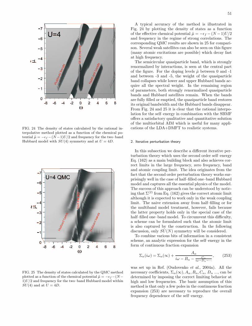
51

FIG. 24 The density of states calculated by the rational in-terpolative method plotted as a function of the chemical po-tential µ = −εf −(N −1)U/2 and frequency for the two–bandHubbard model with SU(4) symmetry and at U = 4D.

FIG. 25 The density of states calculated by the QMC methodplotted as a function of the chemical potential µ = −εf −(N−

1)U/2 and frequency for the two–band Hubbard model withinSU(4) and at U = 4D.

A typical accuracy of the method is illustrated inFig. 24 by plotting the density of states as a functionof the effective chemical potential µ = −εf − (N − 1)U/2and frequency in the regime of strong correlations. Thecorresponding QMC results are shown in 25 for compari-son. Several weak satellites can also be seen on this figure(many atomic excitations are possible) which decay fastat high frequency.

The semicircular quasiparticle band, which is stronglyrenormalized by interactions, is seen at the central partof the figure. For the doping levels µ between 0 and -1and between -3 and -5, the weight of the quasiparticleband collapses while lower and upper Hubbard bands ac-quire all the spectral weight. In the remaining regionof parameters, both strongly renormalized quasiparticlebands and Hubbard satellites remain. When the bandsare fully filled or emptied, the quasiparticle band restoresits original bandwidth and the Hubbard bands disappear.From Fig. 24 and 25 it is clear that the rational interpo-lation for the self–energy in combination with the SBMFoffers a satisfactory qualitative and quantitative solutionof the multiorbital AIM which is useful for many appli-cations of the LDA+DMFT to realistic systems.

2. Iterative perturbation theory

In this subsection we describe a different iterative per-turbation theory which uses the second order self–energyEq. (162) as a main building block and also achieves cor-rect limits in the large frequency, zero frequency, bandand atomic coupling limit. The idea originates from thefact that the second order perturbation theory works sur-prisingly well in the case of half–filled one–band Hubbardmodel and captures all the essential physics of the model.The success of this approach can be understood by notic-ing that Σ(2) from Eq. (162) gives the correct atomic limitalthough it is expected to work only in the weak couplinglimit. The naive extension away from half–filling or forthe multiband model treatment, however, fails becausethe latter property holds only in the special case of thehalf–filled one–band model. To circumvent this difficulty,a scheme can be formulated such that the atomic limitis also captured by the construction. In the followingdiscussion, only SU(N) symmetry will be considered.

To combine various bits of information in a consistentscheme, an analytic expression for the self–energy in theform of continuous fraction expansion

Σα(iω) = Σα(∞) +Aα

iω −Bα − Cα

iω−Dα−···

, (253)

was set up in Ref. (Oudovenko et al., 2004a). All thenecessary coefficients, Σα(∞), Aα, Bα, Cα, Dα ..., can bedetermined by imposing the correct limiting behavior athigh and low frequencies. The basic assumption of thismethod is that only a few poles in the continuous fractionexpansion (253) are necessary to reproduce the overallfrequency dependence of the self–energy.

52

Let us continue by examining the atomic limit of thesecond order self–energy Eq. (162) when evaluated interms of the bare propagator G0

β(iω) = 1/(iω+ µ0 −∆β)

Σ(2)α ∆→0 =

γα

iω + µ0, (254)

where γα =∑

β(Uαβ)2n0β(1 − n0

β) and n0β is a fictitious

particle number

n0β =

1

π

∫f(ω)ImG0

β(ω − i0+)dω, (255)

associated with bare propagator. The choice of µ0 willbe discussed later.

The continuous fraction expansion in Eq. (253) can bemade exact in the restricted atomic limit, i.e., when thethree significant poles are considered in the Green’s func-tion, and coefficients are calculated from the moments of

the self–energy. By replacing iω with γα/Σ(2)α − µ0 in

expansion Eq. (253), it is clear from Eq. (254) that theresulting self–energy functional has the correct atomiclimit and reads

Σα(iω) = Σα(∞)+

Aα

γαΣ

(2)α

1 − eµ0+Bα

γαΣ

(2)α − (Cα/γ2

a)“Σ

(2)α

”2

1−(eµ0+Dα)Σ(2)α /γα−···

.

(256)Coefficients A, B, C and D can be determined from themoment expansion

Aα = Σ(1)α , (257)

Bα =Σ

(2)α

Σ(1)α

, (258)

Cα =Σ

(3)α Σ

(1)α − (Σ

(2)α )2

(Σ(1)α )2

, (259)

where the self–energy moments can be expressed interms of the density–density correlation functions (seeRef. (Oudovenko et al., 2004a)).

Finally, the parameter µ0 can be determined by impos-ing the Friedel sum rule, which is a relation between thetotal density and the real part of the self–energy at zerofrequency, thereby achieving the correct zero frequencylimit. Since the Friedel sum rule is valid only at zero tem-perature, the parameter µ0 is determined at T = 0, andafter having it fixed, equation (256) is used at arbitrarytemperatures.

An alternative scheme for determining thetemperature–dependent µ0 was proposed by Pot-thoff et al. (Potthoff et al., 1997), and consists of therequirement that the fictitious occupancy computedfrom G0 equals the true occupancy computed from G(Martın-Rodero et al., 1982). A careful comparison

of these approaches was carried out by Potthoff et al.(Meyer et al., 1999; Potthoff et al., 1997).

Note that one could continue the expansion in contin-uous fraction to the order in which the expansion givesnot only restricted but the true atomic limit. However, inpractice this is seldom necessary because only few polesclose to the Fermi energy have a large weight.

It is essential that the self–energy Eq. (256) remainsexact to U2, which can be easily verified by noting thatin the U → 0 the fictitious occupancy n0 approaches ntherefore Aα = γα(1 +O(U)), B → −µ0 and C → 0. Atthe same time, the self–energy Eq. (256) has correct firstmoment because expanding Σ(2) in the high–frequency

limit yields Σ(2)α = γα/(iω) + ... and Aα is exact first

moment.Note that in the case of one–band model, the atomic

limit requires only one pole in self–energy therefore thecoefficient C in Eq. (256) can be set to zero and one has

Σα(iω) = Σα(∞) +

Aα

γαΣ

(2)α

1 − eµ0+Bα

γαΣ

(2)α

. (260)

Furthermore, double and triple occupancies do not enterthe expression for the moments in the case of one–bandmodel. If one chooses the functional form for the mo-ments in the atomic limit, the interpolative self–energy(256) has still the same limiting behavior as discussedabove. In this case, no additional external information isnecessary and the system of equations (260), (257), (258)and (162) is closed.

1n

0

0.2

0.4

Z

QMC U=3QMC U=5IPT U=5IPT U=3

FIG. 26 Comparison between QMC and the simplified IPTEq. (260) renormalization amplitude Z for the three–bandHubbard model on Bethe lattice at U = 3D and 5D. QMCZ was extracted at temperature T = 1/16 and IPT at zerotemperature.

For the multiband model, an approximate method isneeded to calculate moments which in turn ensure a lim-iting form consistent with the simplified atomic limit.Many approaches discussed in previous sections can beused for that purpose, for example the Gutzwiller method

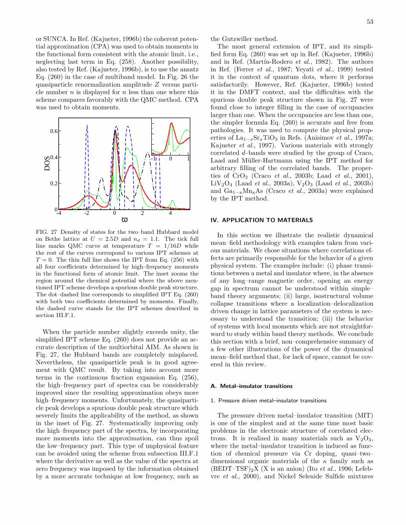
53

or SUNCA. In Ref. (Kajueter, 1996b) the coherent poten-tial approximation (CPA) was used to obtain moments inthe functional form consistent with the atomic limit, i.e.,neglecting last term in Eq. (258). Another possibility,also tested by Ref. (Kajueter, 1996b), is to use the ansatzEq. (260) in the case of multiband model. In Fig. 26 thequasiparticle renormalization amplitude Z versus parti-cle number n is displayed for n less than one where thisscheme compares favorably with the QMC method. CPAwas used to obtain moments.

-4 -2 0 2 4ω

0

0.2

0.4

0.6

DO

S -1 0 1

FIG. 27 Density of states for the two–band Hubbard modelon Bethe lattice at U = 2.5D and nd = 1.1. The tick fullline marks QMC curve at temperature T = 1/16D whilethe rest of the curves correspond to various IPT schemes atT = 0. The thin full line shows the IPT from Eq. (256) withall four coefficients determined by high–frequency momentsin the functional form of atomic limit. The inset zooms theregion around the chemical potential where the above men-tioned IPT scheme develops a spurious double peak structure.The dot–dashed line corresponds to simplified IPT Eq. (260)with both two coefficients determined by moments. Finally,the dashed curve stands for the IPT schemes described insection III.F.1.

When the particle number slightly exceeds unity, thesimplified IPT scheme Eq. (260) does not provide an ac-curate description of the multiorbital AIM. As shown inFig. 27, the Hubbard bands are completely misplaced.Nevertheless, the quasiparticle peak is in good agree-ment with QMC result. By taking into account moreterms in the continuous fraction expansion Eq. (256),the high–frequency part of spectra can be considerablyimproved since the resulting approximation obeys morehigh–frequency moments. Unfortunately, the quasiparti-cle peak develops a spurious double peak structure whichseverely limits the applicability of the method, as shownin the inset of Fig. 27. Systematically improving onlythe high–frequency part of the spectra, by incorporatingmore moments into the approximation, can thus spoilthe low–frequency part. This type of unphysical featurecan be avoided using the scheme from subsection III.F.1where the derivative as well as the value of the spectra atzero frequency was imposed by the information obtainedby a more accurate technique at low frequency, such as

the Gutzwiller method.The most general extension of IPT, and its simpli-

fied form Eq. (260) was set up in Ref. (Kajueter, 1996b)and in Ref. (Martın-Rodero et al., 1982). The authorsin Ref. (Ferrer et al., 1987; Yeyati et al., 1999) testedit in the context of quantum dots, where it performssatisfactorily. However, Ref. (Kajueter, 1996b) testedit in the DMFT context, and the difficulties with thespurious double peak structure shown in Fig. 27 werefound close to integer filling in the case of occupancieslarger than one. When the occupancies are less than one,the simpler formula Eq. (260) is accurate and free frompathologies. It was used to compute the physical prop-erties of La1−xSrxTiO3 in Refs. (Anisimov et al., 1997a;Kajueter et al., 1997). Various materials with stronglycorrelated d–bands were studied by the group of Craco,Laad and Muller-Hartmann using the IPT method forarbitrary filling of the correlated bands. The proper-ties of CrO2 (Craco et al., 2003b; Laad et al., 2001),LiV2O4 (Laad et al., 2003a), V2O3 (Laad et al., 2003b)and Ga1−xMnxAs (Craco et al., 2003a) were explainedby the IPT method.

IV. APPLICATION TO MATERIALS

In this section we illustrate the realistic dynamicalmean–field methodology with examples taken from vari-ous materials. We chose situations where correlations ef-fects are primarily responsible for the behavior of a givenphysical system. The examples include: (i) phase transi-tions between a metal and insulator where, in the absenceof any long–range magnetic order, opening an energygap in spectrum cannot be understood within simple–band theory arguments; (ii) large, isostructural volumecollapse transitions where a localization–delocalizationdriven change in lattice parameters of the system is nec-essary to understand the transition; (iii) the behaviorof systems with local moments which are not straightfor-ward to study within band theory methods. We concludethis section with a brief, non–comprehensive summary ofa few other illustrations of the power of the dynamicalmean–field method that, for lack of space, cannot be cov-ered in this review.

A. Metal–insulator transitions

1. Pressure driven metal–insulator transitions

The pressure driven metal–insulator transition (MIT)is one of the simplest and at the same time most basicproblems in the electronic structure of correlated elec-trons. It is realized in many materials such as V2O3,where the metal–insulator transition is induced as func-tion of chemical pressure via Cr doping, quasi–two–dimensional organic materials of the κ family such as(BEDT–TSF)2X (X is an anion) (Ito et al., 1996; Lefeb-vre et al., 2000), and Nickel Selenide Sulfide mixtures

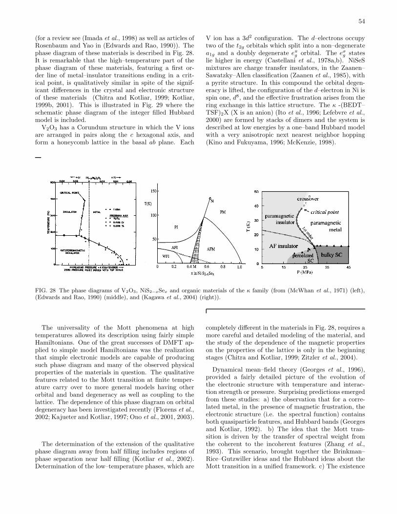
54

(for a review see (Imada et al., 1998) as well as articles ofRosenbaum and Yao in (Edwards and Rao, 1990)). Thephase diagram of these materials is described in Fig. 28.It is remarkable that the high–temperature part of thephase diagram of these materials, featuring a first or-der line of metal–insulator transitions ending in a crit-ical point, is qualitatively similar in spite of the signif-icant differences in the crystal and electronic structureof these materials (Chitra and Kotliar, 1999; Kotliar,1999b, 2001). This is illustrated in Fig. 29 where theschematic phase diagram of the integer filled Hubbardmodel is included.

V2O3 has a Corundum structure in which the V ionsare arranged in pairs along the c hexagonal axis, andform a honeycomb lattice in the basal ab plane. Each

V ion has a 3d2 configuration. The d–electrons occupytwo of the t2g orbitals which split into a non–degeneratea1g and a doubly degenerate eπ

g orbital. The eσg states

lie higher in energy (Castellani et al., 1978a,b). NiSeSmixtures are charge transfer insulators, in the Zaanen–Sawatzky–Allen classification (Zaanen et al., 1985), witha pyrite structure. In this compound the orbital degen-eracy is lifted, the configuration of the d–electron in Ni isspin one, d8, and the effective frustration arises from thering exchange in this lattice structure. The κ -(BEDT–TSF)2X (X is an anion) (Ito et al., 1996; Lefebvre et al.,2000) are formed by stacks of dimers and the system isdescribed at low energies by a one–band Hubbard modelwith a very anisotropic next nearest neighbor hopping(Kino and Fukuyama, 1996; McKenzie, 1998).

FIG. 28 The phase diagrams of V2O3, NiS2−xSex and organic materials of the κ family (from (McWhan et al., 1971) (left),(Edwards and Rao, 1990) (middle), and (Kagawa et al., 2004) (right)).

The universality of the Mott phenomena at hightemperatures allowed its description using fairly simpleHamiltonians. One of the great successes of DMFT ap-plied to simple model Hamiltonians was the realizationthat simple electronic models are capable of producingsuch phase diagram and many of the observed physicalproperties of the materials in question. The qualitativefeatures related to the Mott transition at finite temper-ature carry over to more general models having otherorbital and band degeneracy as well as coupling to thelattice. The dependence of this phase diagram on orbitaldegeneracy has been investigated recently (Florens et al.,2002; Kajueter and Kotliar, 1997; Ono et al., 2001, 2003).

The determination of the extension of the qualitativephase diagram away from half filling includes regions ofphase separation near half filling (Kotliar et al., 2002).Determination of the low–temperature phases, which are

completely different in the materials in Fig. 28, requires amore careful and detailed modeling of the material, andthe study of the dependence of the magnetic propertieson the properties of the lattice is only in the beginningstages (Chitra and Kotliar, 1999; Zitzler et al., 2004).

Dynamical mean–field theory (Georges et al., 1996),provided a fairly detailed picture of the evolution ofthe electronic structure with temperature and interac-tion strength or pressure. Surprising predictions emergedfrom these studies: a) the observation that for a corre-lated metal, in the presence of magnetic frustration, theelectronic structure (i.e. the spectral function) containsboth quasiparticle features, and Hubbard bands (Georgesand Kotliar, 1992). b) The idea that the Mott tran-sition is driven by the transfer of spectral weight fromthe coherent to the incoherent features (Zhang et al.,1993). This scenario, brought together the Brinkman–Rice–Gutzwiller ideas and the Hubbard ideas about theMott transition in a unified framework. c) The existence

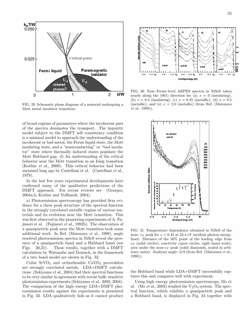
55

FIG. 29 Schematic phase diagram of a material undergoing aMott metal–insulator transition.

of broad regions of parameters where the incoherent partof the spectra dominates the transport. The impuritymodel subject to the DMFT self–consistency conditionis a minimal model to approach the understanding of theincoherent or bad metal, the Fermi liquid state, the Mottinsulating state, and a “semiconducting” or “bad insula-tor” state where thermally induced states populate theMott Hubbard gap. d) An understanding of the criticalbehavior near the Mott transition as an Ising transition(Kotliar et al., 2000). This critical behavior had beensurmised long ago by Castellani et al. (Castellani et al.,1979).

In the last few years experimental developments haveconfirmed many of the qualitative predictions of theDMFT approach. For recent reviews see (Georges,2004a,b; Kotliar and Vollhardt, 2004).

a) Photoemission spectroscopy has provided firm evi-dence for a three peak structure of the spectral functionin the strongly correlated metallic regime of various ma-terials and its evolution near the Mott transition. Thiswas first observed in the pioneering experiments of A. Fu-jimori et al. (Fujimori et al., 1992b). The observation ofa quasiparticle peak near the Mott transition took someadditional work. In Ref. (Matsuura et al., 1998), angleresolved photoemission spectra in NiSeS reveal the pres-ence of a quasiparticle band and a Hubbard band (seeFigs. 30,31). These results, together with a DMFTcalculation by Watanabe and Doniach, in the frameworkof a two–band model are shown in Fig. 32.

Cubic SrVO3 and orthorhombic CaVO3 perovskitesare strongly correlated metals. LDA+DMFT calcula-tions (Sekiyama et al., 2004) find their spectral functionsto be very similar in agreement with recent bulk–sensitivephotoemission experiments (Sekiyama et al., 2002, 2004).The comparison of the high–energy LDA+DMFT pho-toemission results against the experiments is presentedin Fig. 33. LDA qualitatively fails as it cannot produce

FIG. 30 Near–Fermi–level ARPES spectra in NiSeS takennearly along the (001) direction for (a) x = 0 (insulating),(b) x = 0.4 (insulating), (c) x = 0.45 (metallic), (d) x = 0.5(metallic), and (e) x = 2.0 (metallic) (from Ref. (Matsuuraet al., 1998)).

FIG. 31 Temperature–dependence obtained in NiSeS of thenear- εF peak for x = 0.45 at 22.4 eV incident photon energy.Inset: Distance of the 50% point of the leading edge fromεF (solid circles); reactivity (open circles, right–hand scale);area under the near-εF peak (solid diamonds, scaled in arbi-trary units). Analyzer angle: 0/9 (from Ref. (Matsuura et al.,1998)).

the Hubbard band while LDA+DMFT successfully cap-tures this and compares well with experiment.

Using high–energy photoemission spectroscopy, Mo etal. (Mo et al., 2003) studied the V2O3 system. The spec-tral function, which exhibits a quasiparticle peak anda Hubbard band, is displayed in Fig. 34 together with

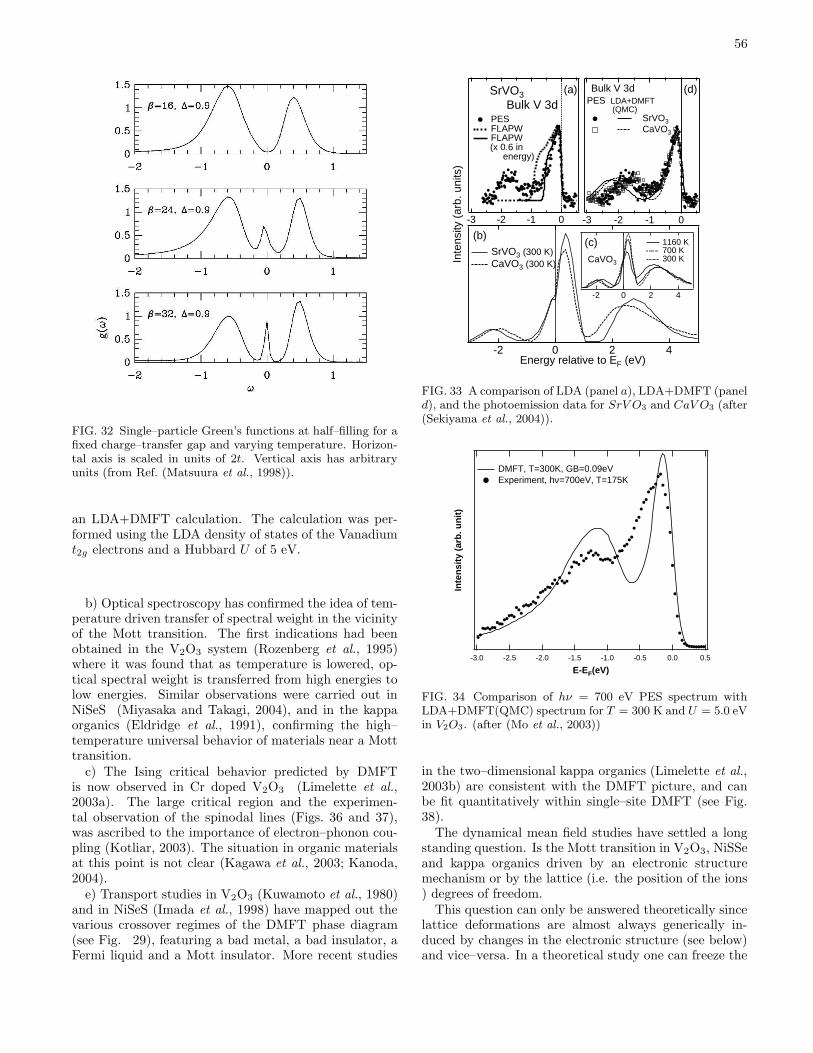
56

FIG. 32 Single–particle Green’s functions at half–filling for afixed charge–transfer gap and varying temperature. Horizon-tal axis is scaled in units of 2t. Vertical axis has arbitraryunits (from Ref. (Matsuura et al., 1998)).

an LDA+DMFT calculation. The calculation was per-formed using the LDA density of states of the Vanadiumt2g electrons and a Hubbard U of 5 eV.

b) Optical spectroscopy has confirmed the idea of tem-perature driven transfer of spectral weight in the vicinityof the Mott transition. The first indications had beenobtained in the V2O3 system (Rozenberg et al., 1995)where it was found that as temperature is lowered, op-tical spectral weight is transferred from high energies tolow energies. Similar observations were carried out inNiSeS (Miyasaka and Takagi, 2004), and in the kappaorganics (Eldridge et al., 1991), confirming the high–temperature universal behavior of materials near a Motttransition.

c) The Ising critical behavior predicted by DMFTis now observed in Cr doped V2O3 (Limelette et al.,2003a). The large critical region and the experimen-tal observation of the spinodal lines (Figs. 36 and 37),was ascribed to the importance of electron–phonon cou-pling (Kotliar, 2003). The situation in organic materialsat this point is not clear (Kagawa et al., 2003; Kanoda,2004).

e) Transport studies in V2O3 (Kuwamoto et al., 1980)and in NiSeS (Imada et al., 1998) have mapped out thevarious crossover regimes of the DMFT phase diagram(see Fig. 29), featuring a bad metal, a bad insulator, aFermi liquid and a Mott insulator. More recent studies

420-2

420-2Energy relative to EF (eV)

1160 K 700 K 300 K

SrVO3 (300 K) CaVO3 (300 K) CaVO3

-3 -2 -1 0 -3 -2 -1 0

Inte

nsity

(ar

b. u

nits

)

(a)

(b)(c)

(d)PES LDA+DMFT (QMC)

SrVO3 CaVO3

SrVO3 Bulk V 3d PES FLAPW FLAPW

(x 0.6 in energy)

Bulk V 3d

FIG. 33 A comparison of LDA (panel a), LDA+DMFT (paneld), and the photoemission data for SrV O3 and CaV O3 (after(Sekiyama et al., 2004)).

Inte

nsi

ty (

arb

. un

it)

-3.0 -2.5 -2.0 -1.5 -1.0 -0.5 0.0 0.5

E-EF(eV)

DMFT, T=300K, GB=0.09eV Experiment, hν=700eV, T=175K

FIG. 34 Comparison of hν = 700 eV PES spectrum withLDA+DMFT(QMC) spectrum for T = 300 K and U = 5.0 eVin V2O3. (after (Mo et al., 2003))

in the two–dimensional kappa organics (Limelette et al.,2003b) are consistent with the DMFT picture, and canbe fit quantitatively within single–site DMFT (see Fig.38).

The dynamical mean field studies have settled a longstanding question. Is the Mott transition in V2O3, NiSSeand kappa organics driven by an electronic structuremechanism or by the lattice (i.e. the position of the ions) degrees of freedom.

This question can only be answered theoretically sincelattice deformations are almost always generically in-duced by changes in the electronic structure (see below)and vice–versa. In a theoretical study one can freeze the

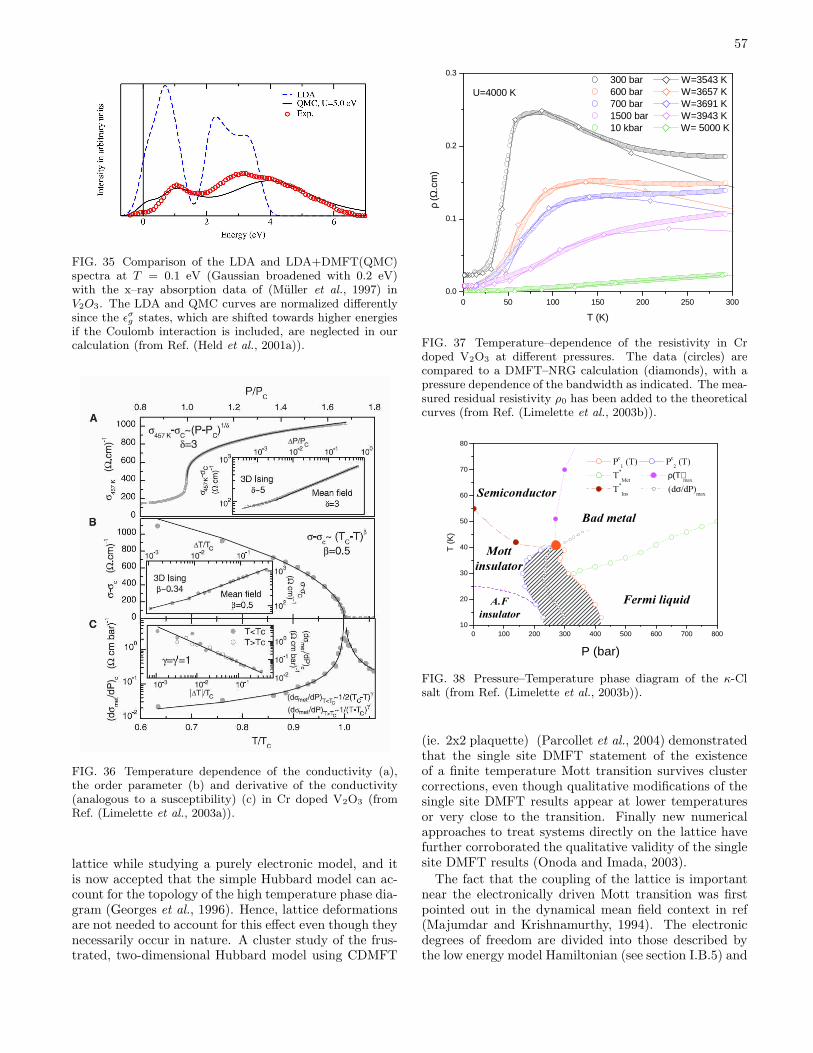
57

FIG. 35 Comparison of the LDA and LDA+DMFT(QMC)spectra at T = 0.1 eV (Gaussian broadened with 0.2 eV)with the x–ray absorption data of (Muller et al., 1997) inV2O3. The LDA and QMC curves are normalized differentlysince the εσ

g states, which are shifted towards higher energiesif the Coulomb interaction is included, are neglected in ourcalculation (from Ref. (Held et al., 2001a)).

FIG. 36 Temperature dependence of the conductivity (a),the order parameter (b) and derivative of the conductivity(analogous to a susceptibility) (c) in Cr doped V2O3 (fromRef. (Limelette et al., 2003a)).

lattice while studying a purely electronic model, and itis now accepted that the simple Hubbard model can ac-count for the topology of the high temperature phase dia-gram (Georges et al., 1996). Hence, lattice deformationsare not needed to account for this effect even though theynecessarily occur in nature. A cluster study of the frus-trated, two-dimensional Hubbard model using CDMFT

0 50 100 150 200 250 3000.0

0.1

0.2

0.3

U=4000 K

ρ (Ω

.cm

)

T (K)

300 bar W=3543 K 600 bar W=3657 K 700 bar W=3691 K 1500 bar W=3943 K 10 kbar W= 5000 K

FIG. 37 Temperature–dependence of the resistivity in Crdoped V2O3 at different pressures. The data (circles) arecompared to a DMFT–NRG calculation (diamonds), with apressure dependence of the bandwidth as indicated. The mea-sured residual resistivity ρ0 has been added to the theoreticalcurves (from Ref. (Limelette et al., 2003b)).

0 100 200 300 400 500 600 700 80010

20

30

40

50

60

70

80

A.Fi n s u l a t o r

SemiconductorB a d meta l

F ermi l iq uid

M ottins ul a tor

P (bar)

T (

K)

Pc1 ( T ) Pc

2 ( T ) T *

M e t ρ(Τ)m a x T *

I n s ( d σ/ d P) m a x

FIG. 38 Pressure–Temperature phase diagram of the κ-Clsalt (from Ref. (Limelette et al., 2003b)).

(ie. 2x2 plaquette) (Parcollet et al., 2004) demonstratedthat the single site DMFT statement of the existenceof a finite temperature Mott transition survives clustercorrections, even though qualitative modifications of thesingle site DMFT results appear at lower temperaturesor very close to the transition. Finally new numericalapproaches to treat systems directly on the lattice havefurther corroborated the qualitative validity of the singlesite DMFT results (Onoda and Imada, 2003).

The fact that the coupling of the lattice is importantnear the electronically driven Mott transition was firstpointed out in the dynamical mean field context in ref(Majumdar and Krishnamurthy, 1994). The electronicdegrees of freedom are divided into those described bythe low energy model Hamiltonian (see section I.B.5) and

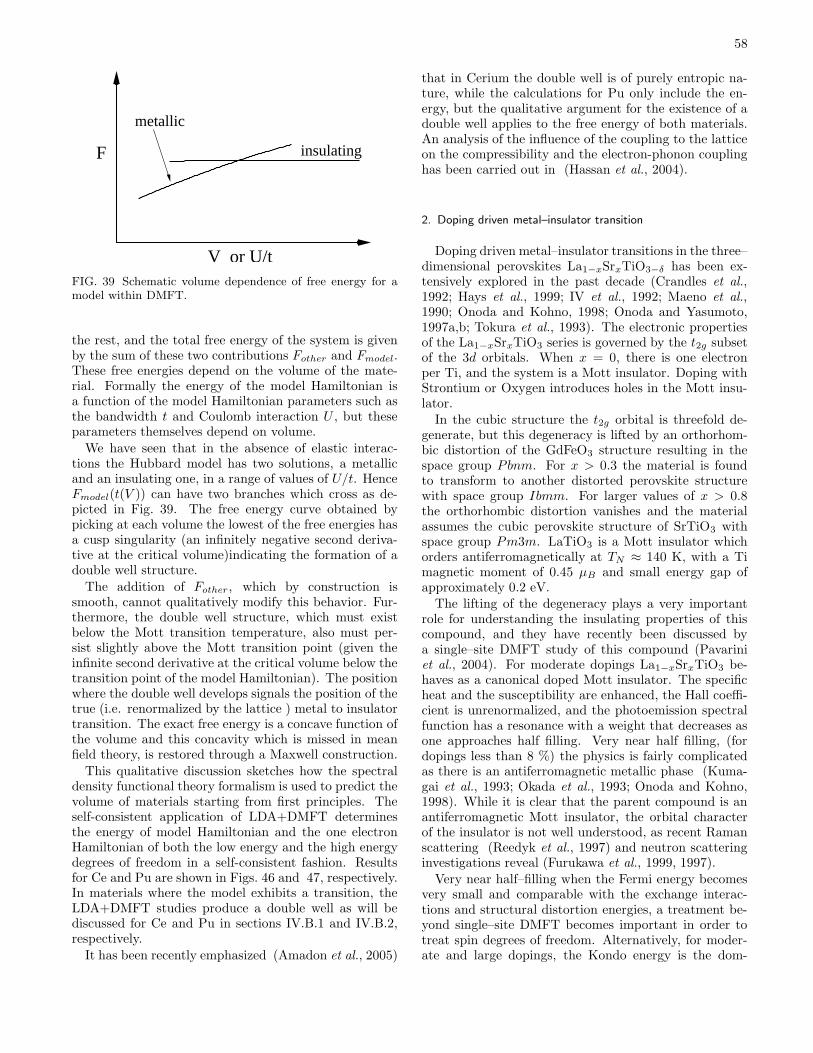
58

metallic

F insulating

V or U/tFIG. 39 Schematic volume dependence of free energy for amodel within DMFT.

the rest, and the total free energy of the system is givenby the sum of these two contributions Fother and Fmodel.These free energies depend on the volume of the mate-rial. Formally the energy of the model Hamiltonian isa function of the model Hamiltonian parameters such asthe bandwidth t and Coulomb interaction U , but theseparameters themselves depend on volume.

We have seen that in the absence of elastic interac-tions the Hubbard model has two solutions, a metallicand an insulating one, in a range of values of U/t. HenceFmodel(t(V )) can have two branches which cross as de-picted in Fig. 39. The free energy curve obtained bypicking at each volume the lowest of the free energies hasa cusp singularity (an infinitely negative second deriva-tive at the critical volume)indicating the formation of adouble well structure.

The addition of Fother, which by construction issmooth, cannot qualitatively modify this behavior. Fur-thermore, the double well structure, which must existbelow the Mott transition temperature, also must per-sist slightly above the Mott transition point (given theinfinite second derivative at the critical volume below thetransition point of the model Hamiltonian). The positionwhere the double well develops signals the position of thetrue (i.e. renormalized by the lattice ) metal to insulatortransition. The exact free energy is a concave function ofthe volume and this concavity which is missed in meanfield theory, is restored through a Maxwell construction.

This qualitative discussion sketches how the spectraldensity functional theory formalism is used to predict thevolume of materials starting from first principles. Theself-consistent application of LDA+DMFT determinesthe energy of model Hamiltonian and the one electronHamiltonian of both the low energy and the high energydegrees of freedom in a self-consistent fashion. Resultsfor Ce and Pu are shown in Figs. 46 and 47, respectively.In materials where the model exhibits a transition, theLDA+DMFT studies produce a double well as will bediscussed for Ce and Pu in sections IV.B.1 and IV.B.2,respectively.

It has been recently emphasized (Amadon et al., 2005)

that in Cerium the double well is of purely entropic na-ture, while the calculations for Pu only include the en-ergy, but the qualitative argument for the existence of adouble well applies to the free energy of both materials.An analysis of the influence of the coupling to the latticeon the compressibility and the electron-phonon couplinghas been carried out in (Hassan et al., 2004).

2. Doping driven metal–insulator transition

Doping driven metal–insulator transitions in the three–dimensional perovskites La1−xSrxTiO3−δ has been ex-tensively explored in the past decade (Crandles et al.,1992; Hays et al., 1999; IV et al., 1992; Maeno et al.,1990; Onoda and Kohno, 1998; Onoda and Yasumoto,1997a,b; Tokura et al., 1993). The electronic propertiesof the La1−xSrxTiO3 series is governed by the t2g subsetof the 3d orbitals. When x = 0, there is one electronper Ti, and the system is a Mott insulator. Doping withStrontium or Oxygen introduces holes in the Mott insu-lator.

In the cubic structure the t2g orbital is threefold de-generate, but this degeneracy is lifted by an orthorhom-bic distortion of the GdFeO3 structure resulting in thespace group Pbnm. For x > 0.3 the material is foundto transform to another distorted perovskite structurewith space group Ibmm. For larger values of x > 0.8the orthorhombic distortion vanishes and the materialassumes the cubic perovskite structure of SrTiO3 withspace group Pm3m. LaTiO3 is a Mott insulator whichorders antiferromagnetically at TN ≈ 140 K, with a Timagnetic moment of 0.45 µB and small energy gap ofapproximately 0.2 eV.

The lifting of the degeneracy plays a very importantrole for understanding the insulating properties of thiscompound, and they have recently been discussed bya single–site DMFT study of this compound (Pavariniet al., 2004). For moderate dopings La1−xSrxTiO3 be-haves as a canonical doped Mott insulator. The specificheat and the susceptibility are enhanced, the Hall coeffi-cient is unrenormalized, and the photoemission spectralfunction has a resonance with a weight that decreases asone approaches half filling. Very near half filling, (fordopings less than 8 %) the physics is fairly complicatedas there is an antiferromagnetic metallic phase (Kuma-gai et al., 1993; Okada et al., 1993; Onoda and Kohno,1998). While it is clear that the parent compound is anantiferromagnetic Mott insulator, the orbital characterof the insulator is not well understood, as recent Ramanscattering (Reedyk et al., 1997) and neutron scatteringinvestigations reveal (Furukawa et al., 1999, 1997).

Very near half–filling when the Fermi energy becomesvery small and comparable with the exchange interac-tions and structural distortion energies, a treatment be-yond single–site DMFT becomes important in order totreat spin degrees of freedom. Alternatively, for moder-ate and large dopings, the Kondo energy is the dom-

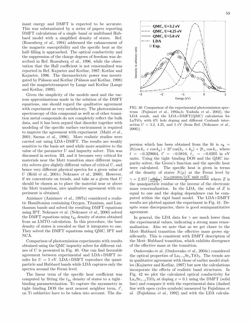
59

inant energy and DMFT is expected to be accurate.This was substantiated by a series of papers reportingDMFT calculations of a single–band or multiband Hub-bard model with a simplified density of states. Ref.(Rozenberg et al., 1994) addressed the enhancement ofthe magnetic susceptibility and the specific heat as thehalf–filling is approached. The optical conductivity andthe suppression of the charge degrees of freedom was de-scribed in Ref. Rozenberg et al., 1996, while the obser-vation that the Hall coefficient is not renormalized wasreported in Ref. Kajueter and Kotliar, 1997; Kotliar andKajueter, 1996. The thermoelectric power was investi-gated by Palsson and Kotliar (Palsson and Kotliar, 1998)and the magnetotransport by Lange and Kotliar (Langeand Kotliar, 1999).

Given the simplicity of the models used and the var-ious approximations made in the solution of the DMFTequations, one should regard the qualitative agreementwith experiment as very satisfactory. The photoemissionspectroscopy of this compound as well as of other transi-tion metal compounds do not completely reflect the bulkdata, and it has been argued that disorder together withmodeling of the specific surface environment is requiredto improve the agreement with experiment (Maiti et al.,2001; Sarma et al., 1996). More realistic studies werecarried out using LDA+DMFT. The results are weaklysensitive to the basis set used while more sensitive to thevalue of the parameter U and impurity solver. This wasdiscussed in section III, and it becomes very critical formaterials near the Mott transition since different impu-rity solvers give slightly different values of critical U , andhence very different physical spectra for a given value ofU (Held et al., 2001c; Nekrasov et al., 2000). However,if we concentrate on trends, and take as a given that Ushould be chosen as to place the material near or abovethe Mott transition, nice qualitative agreement with ex-periment is obtained.

Anisimov (Anisimov et al., 1997a) considered a realis-tic Hamiltonian containing Oxygen, Titanium, and Lan-thanum bands and solved the resulting DMFT equationsusing IPT. Nekrasov et al. (Nekrasov et al., 2000) solvedthe DMFT equations using t2g density of states obtainedfrom an LMTO calculation. In this procedure, the baredensity of states is rescaled so that it integrates to one.They solved the DMFT equations using QMC, IPT andNCA.

Comparison of photoemission experiments with resultsobtained using the QMC impurity solver for different val-ues of U is presented in Fig. 40. One can find favorableagreement between experimental and LDA+DMFT re-sults for U = 5 eV. LDA+DMFT reproduce the quasi-particle and Hubbard bands while LDA captures only thespectra around the Fermi level.

The linear term of the specific heat coefficient wascomputed by fitting the t2g density of states to a tight–binding parameterization. To capture the asymmetry intight–binding DOS the next nearest neighbor term, t′,on Ti sublattice have to be taken into account. The dis-

−3 −2 −1 0 1Energy (eV)

Inte

nsity

in a

rbitr

ary

units

QMC, U=3.2 eVQMC, U=4.25 eVQMC, U=5.0 eVLDAExp.

FIG. 40 Comparison of the experimental photoemission spec-trum (Fujimori et al., 1992a,b; Yoshida et al., 2002), theLDA result, and the LDA+DMFT(QMC) calculation forLaTiO3 with 6% hole doping and different Coulomb inter-action U = 3.2, 4.25, and 5 eV (from Ref. (Nekrasov et al.,2000)).

persion which has been obtained from the fit is εk =2t(cos kx + cos ky) + 2t′ cos(kx + ky) + 2t⊥ cos kz, wheret = −0.329664, t′ = −0.0816, t⊥ = −0.0205 in eVunits. Using the tight–binding DOS and the QMC im-purity solver, the Green’s function and the specific heatwere calculated. The specific heat is given in termsof the density of states N(µ) at the Fermi level by

γ = 2.357[

mJmolK2

] N(µ)[states/(eV unit cell)]Z where Z is

the quasiparticle residue or the inverse of the electronicmass renormalization. In the LDA, the value of Z isequal to one and the doping dependence can be com-puted within the rigid band model. The LDA+DMFTresults are plotted against the experiment in Fig. 41. De-spite some discrepancies, there is good semiquantitativeagreement.

In general, the LDA data for γ are much lower thanthe experimental values, indicating a strong mass renor-malization. Also we note that as we get closer to theMott–Hubbard transition the effective mass grows sig-nificantly. This is consistent with DMFT description ofthe Mott–Hubbard transition, which exhibits divergenceof the effective mass at the transition.

Oudovenko et al. (Oudovenko et al., 2004c) consideredthe optical properties of La1−xSrxTiO3. The trends arein qualitative agreement with those of earlier model stud-ies (Kajueter and Kotliar, 1997) but now the calculationsincorporate the effects of realistic band structures. InFig. 42 we plot the calculated optical conductivity forLaxSr1−xTiO3 at doping x = 0.1 using the DMFT (solidline) and compare it with the experimental data (dashedline with open cycles symbols) measured by Fujishima etal. (Fujishima et al., 1992) and with the LDA calcula-

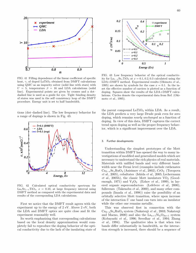
60

0.7 0.8 0.9n

0

10

20γ

experimentQMCLDA

FIG. 41 Filling dependence of the linear coefficient of specificheat, γ, of doped LaTiO3 obtained from DMFT calculationsusing QMC as an impurity solver (solid line with stars) withU = 5, temperature β = 16 and LDA calculations (solidline). Experimental points are given by crosses and a dot–dashed line is used as a guide for eye. Tight–binding densityof states was used in the self–consistency loop of the DMFTprocedure. Energy unit is set to half bandwidth.

tions (dot–dashed line). The low frequency behavior fora range of dopings is shown in Fig. 43.

0 4 8 12Energy, Ev

0

0.2

0.4

0.6

σ, x

106 (m

xΩ)−1

δ=0.1 (DMFT)LDAδ=0.1 (exp)

FIG. 42 Calculated optical conductivity spectrum forLaxSr1−xTiO3, x = 0.10, at large frequency interval usingDMFT method as compared with the experimental data andresults of the corresponding LDA calculations.

First we notice that the DMFT result agrees with theexperiment up to the energy of 2 eV. Above 2 eV, boththe LDA and DMFT optics are quite close and fit theexperiment reasonably well.

Its worth emphasizing that corresponding calculationsbased on the local density approximation would com-pletely fail to reproduce the doping behavior of the opti-cal conductivity due to the lack of the insulating state of

0 0.1 0.2x0

0.2

0.4

Nef

f

experimentDMFT

0 0.5 1Energy (Ev)

0

0.05

0.1

0.15

0.2

σ (1

06 S/m

)

x=0.1x=0.1x=0.2x=0.3

FIG. 43 Low frequency behavior of the optical conductiv-ity for La1−xSrxTiO3 at x = 0.1, 0.2, 0.3 calculated using theLDA+DMFT method. Experimental results (Okimoto et al.,1995) are shown by symbols for the case x = 0.1. In the in-set the effective number of carriers is plotted as a function ofdoping. Squares show the results of the LDA+DMFT calcu-lations. Circles denote the experimental data from Ref. (Oki-moto et al., 1995).

the parent compound LaTiO3 within LDA. As a result,the LDA predicts a very large Drude peak even for zerodoping, which remains nearly unchanged as a function ofdoping. In view of this data, DMFT captures the correcttrend upon doping as well as the proper frequency behav-ior, which is a significant improvement over the LDA.

3. Further developments

Understanding the simplest prototypes of the Motttransition within DMFT has opened the way to many in-vestigations of modified and generalized models which arenecessary to understand the rich physics of real materials.Materials with unfilled bands and very different band-width near the Fermi level (examples include ruthenatesCa2−xSrxRuO4 (Anisimov et al., 2002), CrO2 (Toropovaet al., 2005), cobaltates (Ishida et al., 2005; Lechermannet al., 2005b), the classic Mott insulators VO2 (Good-enough, 1971) and V2O3 (Ezhov et al., 1999), in lay-ered organic superconductors (Lefebvre et al., 2000),fullerenes (Takenobu et al., 2000), and many other com-pounds (Imada et al., 1998)) raise the possibility of anorbitally selective Mott transition, where upon increaseof the interaction U one band can turn into an insulatorwhile the other one remains metallic.

This was observed first in connection with theCa2−xSrxRuO4 system (Nakatsuji et al., 2003; Nakatsujiand Maeno, 2000) and also the Lan+1NinO3n+1 system(Kobayashi et al., 1996; Sreedhar et al., 1994; Zhanget al., 1994). The qualitative idea is that when twobands differ substantially in bandwidth, as the interac-tion strength is increased, there should be a sequence of

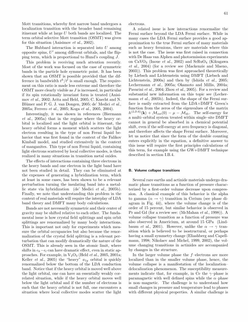
61

Mott transitions, whereby first narrow band undergoes alocalization transition with the broader band remainingitinerant while at large U both bands are localized. Theterm orbital selective Mott transition (OSMT) was givenfor this situation (Anisimov et al., 2002).

The Hubbard interaction is separated into U amongopposite spins, U ′ among different orbitals, and the flip-ping term, which is proportional to Hund’s coupling J .

This problem is receiving much attention recently.Most of the work was focused on the case of symmetricbands in the particle hole symmetric point. It has beenshown that an OSMT is possible provided that the dif-ference in bandwidth th/tl is small enough. The require-ment on this ratio is made less extreme and therefore theOSMT more clearly visible as J is increased, in particularif its spin rotationally invariant form is treated (Anisi-mov et al., 2002; Arita and Held, 2005; C. Knecht and N.Blumer and P. G. J. van Dongen, 2005; de’ Medici et al.,2005a; Ferrero et al., 2005; Koga et al., 2005, 2004).

Interestingly, it was shown in references (Biermannet al., 2005a) that in the regime where the heavy or-bital is localized and the light orbital is itinerant, theheavy orbital forms a moment which scatters the lightelectron resulting in the type of non Fermi liquid be-havior that was first found in the context of the FalikovKimball model, and studied extensively in the contextof manganites. This type of non Fermi liquid, containinglight electrons scattered by local collective modes, is thenrealized in many situations in transition metal oxides.

The effects of interactions containing three electrons inthe heavy bands and one electron in the light band havenot been studied in detail. They can be eliminated atthe expenses of generating a hybridization term, whichat least in some cases, has been shown to be a relevantperturbation turning the insulating band into a metal-lic state via hybridization (de’ Medici et al., 2005b).Finally, we note that understanding this problem in thecontext of real materials will require the interplay of LDAband theory and DMFT many body calculations.

Bands are not necessarily symmetric and their center ofgravity may be shifted relative to each other. The funda-mental issue is how crystal field splittings and spin orbitsplittings are renormalized by many body interactions.This is important not only for experiments which mea-sure the orbital occupancies but also because the renor-malization of the crystal field splitting is a relevant per-turbation that can modify dramatically the nature of theOSMT. This is already seen in the atomic limit, whereshifts in εh−εl can have dramatic effect, even in static ap-proaches. For example, in V2O3 (Held et al., 2005, 2001a;Keller et al., 2005) the “heavy” a1g orbital is quicklyrenormalized below the bottom of the LDA conductionband. Notice that if the heavy orbital is moved well abovethe light orbital, one can have an essentially weakly cor-related situation, while if the heavy orbital moves wellbelow the light orbital and if the number of electrons issuch that the heavy orbital is not full, one encounters asituation where local collective modes scatter the light

electrons.A related issue is how interactions renormalize the

Fermi surface beyond the LDA Fermi surface. While inmany cases the LDA Fermi surface provides a good ap-proximation to the true Fermi surface of many materialssuch as heavy fermions, there are materials where thisis not the case. The issue was first raised in connectionwith De Haas van Alphen and photoemission experimentson CaVO3 (Inoue et al., 2002) and SrRuO4 (Kikugawaet al., 2004) (for a review see (Mackenzie and Maeno,2003)). This problem was first approached theoreticallyby Liebsch and Lichtenstein using DMFT (Liebsch andLichtenstein, 2000a) and then by (Ishida et al., 2005;Lechermann et al., 2005a; Okamoto and Millis, 2004a;Pavarini et al., 2004; Zhou et al., 2005). For a review andsubstantial new information on this topic see (Lecher-mann et al., 2005b). Indeed, the shape of the Fermi sur-face is easily extracted from the LDA+DMFT Green’sfunction from the zeros of the eigenvalues of the matrixh(LDA)(k) + Mint(0) − µ − Mdc. The self-energy fora multi–orbital system treated within single–site DMFTcannot in general be absorbed in a chemical potentialshift, even if the self-energy at zero frequency is diagonal,and therefore affects the shape Fermi surface. Moreover,let us notice that since the form of the double countingenters explicitly in the equation, a definitive answer tothis issue will require the first principles calculations ofthis term, for example using the GW+DMFT techniquedescribed in section I.B.4.

B. Volume collapse transitions

Several rare earths and actinide materials undergo dra-matic phase transitions as a function of pressure charac-terized by a first-order volume decrease upon compres-sion. A classical example of this behavior is the alphato gamma (α → γ) transition in Cerium (see phase di-agram in Fig. 44), where the volume change is of theorder of 15 percent, but similar behavior is observed inPr and Gd (for a review see: (McMahan et al., 1998)). Avolume collapse transition as a function of pressure wasalso observed in Americium, at around 15 GPa (Lind-baum et al., 2001). However, unlike the α → γ tran-sition which is believed to be isostructural, or perhapshaving a small symmetry change (Eliashberg and Capell-mann, 1998; Nikolaev and Michel, 1999, 2002), the vol-ume changing transitions in actinides are accompaniedby changes in the structure.

In the larger volume phase the f–electrons are morelocalized than in the smaller volume phase, hence, thevolume collapse is a manifestation of the localization–delocalization phenomenon. The susceptibility measure-ments indicate that, for example, in Ce the γ–phase isparamagnetic with well defined spins while the α–phaseis non–magnetic. The challenge is to understand howsmall changes in pressure and temperature lead to phaseswith different physical properties. A similar challenge is

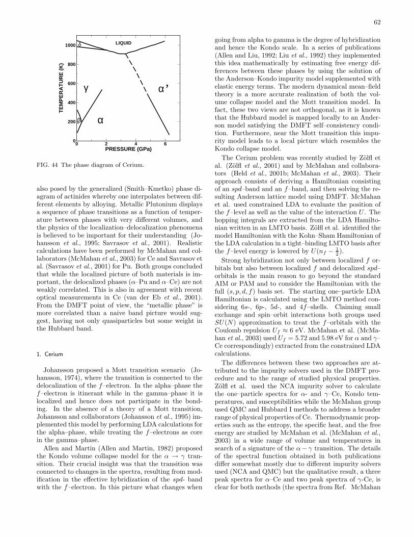
62

0 2 4 6PRESSURE (GPa)

0

200

400

600

800

1000

TE

MP

ER

AT

UR

E (

K)

LIQUID

α

α

β

δ

γ ’

FIG. 44 The phase diagram of Cerium.

also posed by the generalized (Smith–Kmetko) phase di-agram of actinides whereby one interpolates between dif-ferent elements by alloying. Metallic Plutonium displaysa sequence of phase transitions as a function of temper-ature between phases with very different volumes, andthe physics of the localization–delocalization phenomenais believed to be important for their understanding (Jo-hansson et al., 1995; Savrasov et al., 2001). Realisticcalculations have been performed by McMahan and col-laborators (McMahan et al., 2003) for Ce and Savrasov etal. (Savrasov et al., 2001) for Pu. Both groups concludedthat while the localized picture of both materials is im-portant, the delocalized phases (α–Pu and α–Ce) are notweakly correlated. This is also in agreement with recentoptical measurements in Ce (van der Eb et al., 2001).From the DMFT point of view, the “metallic phase” ismore correlated than a naive band picture would sug-gest, having not only quasiparticles but some weight inthe Hubbard band.

1. Cerium

Johansson proposed a Mott transition scenario (Jo-hansson, 1974), where the transition is connected to thedelocalization of the f–electron. In the alpha–phase thef–electron is itinerant while in the gamma–phase it islocalized and hence does not participate in the bond-ing. In the absence of a theory of a Mott transition,Johansson and collaborators (Johansson et al., 1995) im-plemented this model by performing LDA calculations forthe alpha–phase, while treating the f–electrons as corein the gamma–phase.

Allen and Martin (Allen and Martin, 1982) proposedthe Kondo volume collapse model for the α → γ tran-sition. Their crucial insight was that the transition wasconnected to changes in the spectra, resulting from mod-ification in the effective hybridization of the spd- bandwith the f–electron. In this picture what changes when

going from alpha to gamma is the degree of hybridizationand hence the Kondo scale. In a series of publications(Allen and Liu, 1992; Liu et al., 1992) they implementedthis idea mathematically by estimating free energy dif-ferences between these phases by using the solution ofthe Anderson–Kondo impurity model supplemented withelastic energy terms. The modern dynamical mean–fieldtheory is a more accurate realization of both the vol-ume collapse model and the Mott transition model. Infact, these two views are not orthogonal, as it is knownthat the Hubbard model is mapped locally to an Ander-son model satisfying the DMFT self–consistency condi-tion. Furthermore, near the Mott transition this impu-rity model leads to a local picture which resembles theKondo collapse model.

The Cerium problem was recently studied by Zolfl etal. (Zolfl et al., 2001) and by McMahan and collabora-tors (Held et al., 2001b; McMahan et al., 2003). Theirapproach consists of deriving a Hamiltonian consistingof an spd–band and an f–band, and then solving the re-sulting Anderson lattice model using DMFT. McMahanet al. used constrained LDA to evaluate the position ofthe f–level as well as the value of the interaction U . Thehopping integrals are extracted from the LDA Hamilto-nian written in an LMTO basis. Zolfl et al. identified themodel Hamiltonian with the Kohn–Sham Hamiltonian ofthe LDA calculation in a tight–binding LMTO basis afterthe f–level energy is lowered by U(nf − 1

2 ).

Strong hybridization not only between localized f or-bitals but also between localized f and delocalized spd–orbitals is the main reason to go beyond the standardAIM or PAM and to consider the Hamiltonian with thefull (s, p, d, f) basis set. The starting one–particle LDAHamiltonian is calculated using the LMTO method con-sidering 6s-, 6p-, 5d-, and 4f–shells. Claiming smallexchange and spin–orbit interactions both groups usedSU(N) approximation to treat the f–orbitals with theCoulomb repulsion Uf ≈ 6 eV. McMahan et al. (McMa-han et al., 2003) used Uf = 5.72 and 5.98 eV for α and γ–Ce correspondingly) extracted from the constrained LDAcalculations.

The differences between these two approaches are at-tributed to the impurity solvers used in the DMFT pro-cedure and to the range of studied physical properties.Zolfl et al. used the NCA impurity solver to calculatethe one–particle spectra for α- and γ–Ce, Kondo tem-peratures, and susceptibilities while the McMahan groupused QMC and Hubbard I methods to address a broaderrange of physical properties of Ce. Thermodynamic prop-erties such as the entropy, the specific heat, and the freeenergy are studied by McMahan et al. (McMahan et al.,2003) in a wide range of volume and temperatures insearch of a signature of the α− γ transition. The detailsof the spectral function obtained in both publicationsdiffer somewhat mostly due to different impurity solversused (NCA and QMC) but the qualitative result, a threepeak spectra for α–Ce and two peak spectra of γ-Ce, isclear for both methods (the spectra from Ref. McMahan

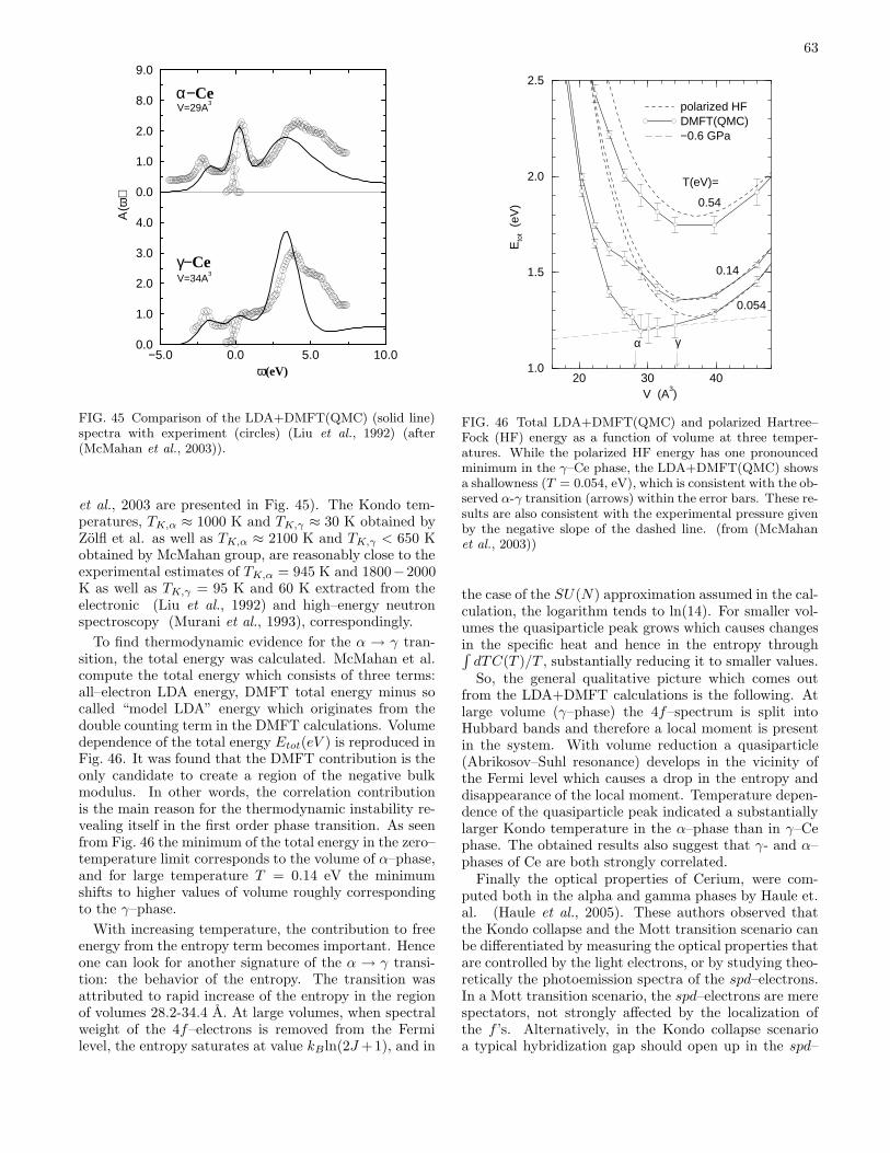
63

−5.0 0.0 5.0 10.0ω(eV)

0.0

1.0

2.0

3.0

4.0

0.0

1.0

2.0

8.0

9.0

Α(ω

)V=29A

3

V=34A3

α−Ce

γ−Ce

FIG. 45 Comparison of the LDA+DMFT(QMC) (solid line)spectra with experiment (circles) (Liu et al., 1992) (after(McMahan et al., 2003)).

et al., 2003 are presented in Fig. 45). The Kondo tem-peratures, TK,α ≈ 1000 K and TK,γ ≈ 30 K obtained byZolfl et al. as well as TK,α ≈ 2100 K and TK,γ < 650 Kobtained by McMahan group, are reasonably close to theexperimental estimates of TK,α = 945 K and 1800−2000K as well as TK,γ = 95 K and 60 K extracted from theelectronic (Liu et al., 1992) and high–energy neutronspectroscopy (Murani et al., 1993), correspondingly.

To find thermodynamic evidence for the α → γ tran-sition, the total energy was calculated. McMahan et al.compute the total energy which consists of three terms:all–electron LDA energy, DMFT total energy minus socalled “model LDA” energy which originates from thedouble counting term in the DMFT calculations. Volumedependence of the total energy Etot(eV ) is reproduced inFig. 46. It was found that the DMFT contribution is theonly candidate to create a region of the negative bulkmodulus. In other words, the correlation contributionis the main reason for the thermodynamic instability re-vealing itself in the first order phase transition. As seenfrom Fig. 46 the minimum of the total energy in the zero–temperature limit corresponds to the volume of α–phase,and for large temperature T = 0.14 eV the minimumshifts to higher values of volume roughly correspondingto the γ–phase.

With increasing temperature, the contribution to freeenergy from the entropy term becomes important. Henceone can look for another signature of the α → γ transi-tion: the behavior of the entropy. The transition wasattributed to rapid increase of the entropy in the regionof volumes 28.2-34.4 A. At large volumes, when spectralweight of the 4f–electrons is removed from the Fermilevel, the entropy saturates at value kB ln(2J+1), and in

20 30 40V (A

3)

1.0

1.5

2.0

2.5

Eto

t (e

V)

polarized HFDMFT(QMC)−0.6 GPa

T(eV)=

0.54

0.14

0.054

α γ

FIG. 46 Total LDA+DMFT(QMC) and polarized Hartree–Fock (HF) energy as a function of volume at three temper-atures. While the polarized HF energy has one pronouncedminimum in the γ–Ce phase, the LDA+DMFT(QMC) showsa shallowness (T = 0.054, eV), which is consistent with the ob-served α-γ transition (arrows) within the error bars. These re-sults are also consistent with the experimental pressure givenby the negative slope of the dashed line. (from (McMahanet al., 2003))

the case of the SU(N) approximation assumed in the cal-culation, the logarithm tends to ln(14). For smaller vol-umes the quasiparticle peak grows which causes changesin the specific heat and hence in the entropy through∫dTC(T )/T , substantially reducing it to smaller values.So, the general qualitative picture which comes out

from the LDA+DMFT calculations is the following. Atlarge volume (γ–phase) the 4f–spectrum is split intoHubbard bands and therefore a local moment is presentin the system. With volume reduction a quasiparticle(Abrikosov–Suhl resonance) develops in the vicinity ofthe Fermi level which causes a drop in the entropy anddisappearance of the local moment. Temperature depen-dence of the quasiparticle peak indicated a substantiallylarger Kondo temperature in the α–phase than in γ–Cephase. The obtained results also suggest that γ- and α–phases of Ce are both strongly correlated.

Finally the optical properties of Cerium, were com-puted both in the alpha and gamma phases by Haule et.al. (Haule et al., 2005). These authors observed thatthe Kondo collapse and the Mott transition scenario canbe differentiated by measuring the optical properties thatare controlled by the light electrons, or by studying theo-retically the photoemission spectra of the spd–electrons.In a Mott transition scenario, the spd–electrons are merespectators, not strongly affected by the localization ofthe f ’s. Alternatively, in the Kondo collapse scenarioa typical hybridization gap should open up in the spd–

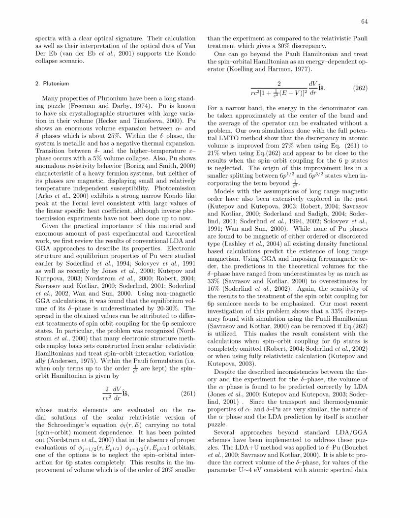
64

spectra with a clear optical signature. Their calculationas well as their interpretation of the optical data of VanDer Eb (van der Eb et al., 2001) supports the Kondocollapse scenario.

2. Plutonium

Many properties of Plutonium have been a long stand-ing puzzle (Freeman and Darby, 1974). Pu is knownto have six crystallographic structures with large varia-tion in their volume (Hecker and Timofeeva, 2000). Pushows an enormous volume expansion between α- andδ–phases which is about 25%. Within the δ–phase, thesystem is metallic and has a negative thermal expansion.Transition between δ- and the higher–temperature ε–phase occurs with a 5% volume collapse. Also, Pu showsanomalous resistivity behavior (Boring and Smith, 2000)characteristic of a heavy fermion systems, but neither ofits phases are magnetic, displaying small and relativelytemperature independent susceptibility. Photoemission(Arko et al., 2000) exhibits a strong narrow Kondo–likepeak at the Fermi level consistent with large values ofthe linear specific heat coefficient, although inverse pho-toemission experiments have not been done up to now.

Given the practical importance of this material andenormous amount of past experimental and theoreticalwork, we first review the results of conventional LDA andGGA approaches to describe its properties. Electronicstructure and equilibrium properties of Pu were studiedearlier by Soderlind et al., 1994; Solovyev et al., 1991as well as recently by Jones et al., 2000; Kutepov andKutepova, 2003; Nordstrom et al., 2000; Robert, 2004;Savrasov and Kotliar, 2000; Soderlind, 2001; Soderlindet al., 2002; Wan and Sun, 2000. Using non–magneticGGA calculations, it was found that the equilibrium vol-ume of its δ–phase is underestimated by 20-30%. Thespread in the obtained values can be attributed to differ-ent treatments of spin orbit coupling for the 6p semicorestates. In particular, the problem was recognized (Nord-strom et al., 2000) that many electronic structure meth-ods employ basis sets constructed from scalar–relativisticHamiltonians and treat spin–orbit interaction variation-ally (Andersen, 1975). Within the Pauli formulation (i.e.when only terms up to the order 1

c2 are kept) the spin–orbit Hamiltonian is given by

2

rc2dV

drls, (261)

whose matrix elements are evaluated on the ra-dial solutions of the scalar relativistic version ofthe Schroedinger’s equation φl(r, E) carrying no total(spin+orbit) moment dependence. It has been pointedout (Nordstrom et al., 2000) that in the absence of properevaluations of φj=1/2(r, Ep1/2) φj=3/2(r, Ep3/2) orbitals,one of the options is to neglect the spin–orbital inter-action for 6p states completely. This results in the im-provement of volume which is of the order of 20% smaller

than the experiment as compared to the relativistic Paulitreatment which gives a 30% discrepancy.

One can go beyond the Pauli Hamiltonian and treatthe spin–orbital Hamiltonian as an energy–dependent op-erator (Koelling and Harmon, 1977).

2

rc2[1 + 1c2 (E − V )]2

dV

drls. (262)

For a narrow band, the energy in the denominator canbe taken approximately at the center of the band andthe average of the operator can be evaluated without aproblem. Our own simulations done with the full poten-tial LMTO method show that the discrepancy in atomicvolume is improved from 27% when using Eq. (261) to21% when using Eq.(262) and appear to be close to theresults when the spin–orbit coupling for the 6 p statesis neglected. The origin of this improvement lies in asmaller splitting between 6p1/2 and 6p3/2 states when in-corporating the term beyond 1

c2 .

Models with the assumptions of long range magneticorder have also been extensively explored in the past(Kutepov and Kutepova, 2003; Robert, 2004; Savrasovand Kotliar, 2000; Soderland and Sadigh, 2004; Soder-lind, 2001; Soderlind et al., 1994, 2002; Solovyev et al.,1991; Wan and Sun, 2000). While none of Pu phasesare found to be magnetic of either ordered or disorderedtype (Lashley et al., 2004) all existing density functionalbased calculations predict the existence of long rangemagnetism. Using GGA and imposing ferromagnetic or-der, the predictions in the theoretical volumes for theδ–phase have ranged from underestimates by as much as33% (Savrasov and Kotliar, 2000) to overestimates by16% (Soderlind et al., 2002). Again, the sensitivity ofthe results to the treatment of the spin orbit coupling for6p semicore needs to be emphasized. Our most recentinvestigation of this problem shows that a 33% discrep-ancy found with simulation using the Pauli Hamiltonian(Savrasov and Kotliar, 2000) can be removed if Eq.(262)is utilized. This makes the result consistent with thecalculations when spin–orbit coupling for 6p states iscompletely omitted (Robert, 2004; Soderlind et al., 2002)or when using fully relativistic calculation (Kutepov andKutepova, 2003).

Despite the described inconsistencies between the the-ory and the experiment for the δ–phase, the volume ofthe α–phase is found to be predicted correctly by LDA(Jones et al., 2000; Kutepov and Kutepova, 2003; Soder-lind, 2001) . Since the transport and thermodynamicproperties of α- and δ–Pu are very similar, the nature ofthe α–phase and the LDA prediction by itself is anotherpuzzle.

Several approaches beyond standard LDA/GGAschemes have been implemented to address these puz-zles. The LDA+U method was applied to δ–Pu (Bouchetet al., 2000; Savrasov and Kotliar, 2000). It is able to pro-duce the correct volume of the δ–phase, for values of theparameter U∼4 eV consistent with atomic spectral data

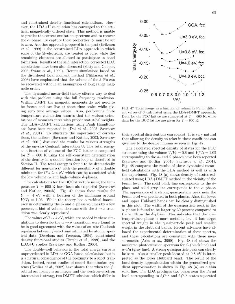
65

and constrained density functional calculations. How-ever, the LDA+U calculation has converged to the arti-ficial magnetically ordered state. This method is unableto predict the correct excitation spectrum and to recoverthe α–phase. To capture these properties, U must be setto zero. Another approach proposed in the past (Erikssonet al., 1999) is the constrained LDA approach in whichsome of the 5f–electrons, are treated as core, while theremaining electrons are allowed to participate in bandformation. Results of the self–interaction–corrected LDAcalculations have been also discussed (Setty and Cooper,2003; Svane et al., 1999). Recent simulations based onthe disordered local moment method (Niklasson et al.,2003) have emphasized that the volume of the δ–Pu canbe recovered without an assumption of long range mag-netic order.

The dynamical mean–field theory offers a way to dealwith the problem using the full frequency resolution.Within DMFT the magnetic moments do not need tobe frozen and can live at short time scales while giv-ing zero time average values. Also, performing finitetemperature calculation ensures that the various orien-tations of moments enter with proper statistical weights.The LDA+DMFT calculations using Pauli Hamiltoni-ans have been reported in (Dai et al., 2003; Savrasovet al., 2001). To illustrate the importance of correla-tions, the authors (Savrasov and Kotliar, 2003; Savrasovet al., 2001) discussed the results for various strengthsof the on–site Coulomb interaction U. The total energyas a function of volume of the FCC lattice is computedfor T = 600 K using the self–consistent determinationof the density in a double iteration loop as described inSection II. The total energy is found to be dramaticallydifferent for non–zero U with the possibility of a doubleminimum for U ′s ∼= 4 eV which can be associated withthe low volume α- and high–volume δ–phases.

The calculations for the BCC structure using the tem-perature T = 900 K have been also reported (Savrasovand Kotliar, 2004b). Fig. 47 shows these results forU = 4 eV with a location of the minimum aroundV/Vδ = 1.03. While the theory has a residual inaccu-racy in determining the δ- and ε–phase volumes by a fewpercent, a hint of volume decrease with the δ → ε tran-sition was clearly reproduced.

The values of U ∼ 4 eV, which are needed in these sim-ulations to describe the α → δ transition, were found tobe in good agreement with the values of on–site Coulombrepulsion between f–electrons estimated by atomic spec-tral data (Desclaux and Freeman, 1984), constraineddensity functional studies (Turchi et al., 1999), and theLDA+U studies (Savrasov and Kotliar, 2000).

The double–well behavior in the total energy curve isunprecedented in LDA or GGA based calculations but itis a natural consequence of the proximity to a Mott tran-sition. Indeed, recent studies of model Hamiltonian sys-tems (Kotliar et al., 2002) have shown that when the f–orbital occupancy is an integer and the electron–electroninteraction is strong, two DMFT solutions which differ in

0.6 0.7 0.8 0.9 1.0 1.1 1.2-0.25

-0.20

-0.15

-0.10

-0.05

0.00

U=4.0 eV, bcc

U=4.0 eV, fcc

GGA, fcc

U=3.0 eV, fcc

U=3.8 eV, fcc

V/Vd

Tota

l E

nerg

y,R

y

FIG. 47 Total energy as a function of volume in Pu for differ-ent values of U calculated using the LDA+DMFT approach.Data for the FCC lattice are computed at T = 600 K, whiledata for the BCC lattice are given for T = 900 K.

their spectral distributions can coexist. It is very naturalthat allowing the density to relax in these conditions cangive rise to the double minima as seen in Fig. 47.

The calculated spectral density of states for the FCCstructure using the volume V/Vδ = 0.8 and V/Vδ = 1.05corresponding to the α- and δ–phases have been reported(Savrasov and Kotliar, 2004b; Savrasov et al., 2001).Fig. 48 compares the results of these dynamical mean–field calculations with the LDA method as well as withthe experiment. Fig. 48 (a) shows density of states cal-culated using LDA+DMFT method in the vicinity of theFermi level. The solid black line corresponds to the δ–phase and solid grey line corresponds to the α–phase.The appearance of a strong quasiparticle peak near theFermi level was predicted in both phases. Also, the lowerand upper Hubbard bands can be clearly distinguishedin this plot. The width of the quasiparticle peak in theα–phase is found to be larger by 30 percent compared tothe width in the δ–phase. This indicates that the low–temperature phase is more metallic, i.e. it has largerspectral weight in the quasiparticle peak and smallerweight in the Hubbard bands. Recent advances have al-lowed the experimental determination of these spectra,and these calculations are consistent with these mea-surements (Arko et al., 2000). Fig. 48 (b) shows themeasured photoemission spectrum for δ- (black line) andα–Pu (gray line). A strong quasiparticle peak can clearlybe seen. Also a smaller peak located at 0.8 eV is inter-preted as the lower Hubbard band. The result of thelocal density approximation within the generalized gra-dient approximation is shown in Fig. 48 (a) as a thinsolid line. The LDA produces two peaks near the Fermilevel corresponding to 5f 5/2 and 5f7/2 states separated

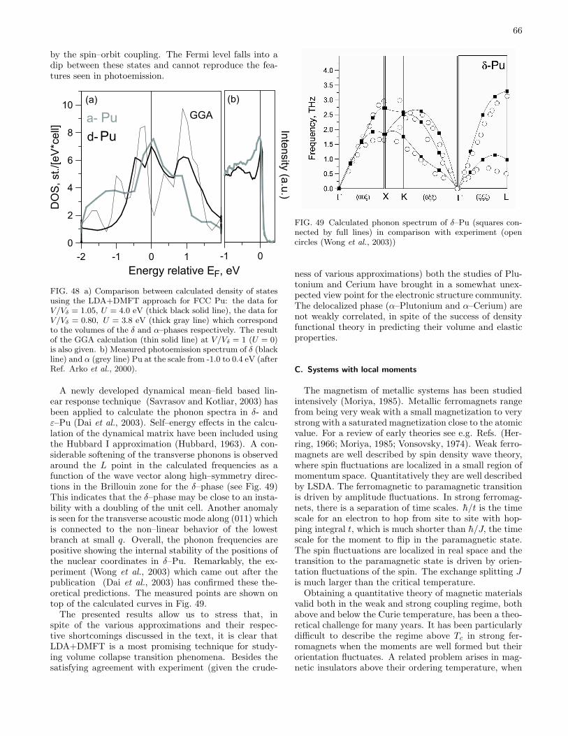
66

by the spin–orbit coupling. The Fermi level falls into adip between these states and cannot reproduce the fea-tures seen in photoemission.

-2 -1 0 1

0

2

4

6

8

10

Energy relative EF, eV

DO

S,

st.

/[e

V*c

ell]

GGA

-1 0

Inte

nsity

(a.u

.)

(a) (b)

a- Pu

d- Pu

FIG. 48 a) Comparison between calculated density of statesusing the LDA+DMFT approach for FCC Pu: the data forV/Vδ = 1.05, U = 4.0 eV (thick black solid line), the data forV/Vδ = 0.80, U = 3.8 eV (thick gray line) which correspondto the volumes of the δ and α–phases respectively. The resultof the GGA calculation (thin solid line) at V/Vδ = 1 (U = 0)is also given. b) Measured photoemission spectrum of δ (blackline) and α (grey line) Pu at the scale from -1.0 to 0.4 eV (afterRef. Arko et al., 2000).

A newly developed dynamical mean–field based lin-ear response technique (Savrasov and Kotliar, 2003) hasbeen applied to calculate the phonon spectra in δ- andε–Pu (Dai et al., 2003). Self–energy effects in the calcu-lation of the dynamical matrix have been included usingthe Hubbard I approximation (Hubbard, 1963). A con-siderable softening of the transverse phonons is observedaround the L point in the calculated frequencies as afunction of the wave vector along high–symmetry direc-tions in the Brillouin zone for the δ–phase (see Fig. 49)This indicates that the δ–phase may be close to an insta-bility with a doubling of the unit cell. Another anomalyis seen for the transverse acoustic mode along (011) whichis connected to the non–linear behavior of the lowestbranch at small q. Overall, the phonon frequencies arepositive showing the internal stability of the positions ofthe nuclear coordinates in δ–Pu. Remarkably, the ex-periment (Wong et al., 2003) which came out after thepublication (Dai et al., 2003) has confirmed these the-oretical predictions. The measured points are shown ontop of the calculated curves in Fig. 49.

The presented results allow us to stress that, inspite of the various approximations and their respec-tive shortcomings discussed in the text, it is clear thatLDA+DMFT is a most promising technique for study-ing volume collapse transition phenomena. Besides thesatisfying agreement with experiment (given the crude-

FIG. 49 Calculated phonon spectrum of δ–Pu (squares con-nected by full lines) in comparison with experiment (opencircles (Wong et al., 2003))

ness of various approximations) both the studies of Plu-tonium and Cerium have brought in a somewhat unex-pected view point for the electronic structure community.The delocalized phase (α–Plutonium and α–Cerium) arenot weakly correlated, in spite of the success of densityfunctional theory in predicting their volume and elasticproperties.

C. Systems with local moments

The magnetism of metallic systems has been studiedintensively (Moriya, 1985). Metallic ferromagnets rangefrom being very weak with a small magnetization to verystrong with a saturated magnetization close to the atomicvalue. For a review of early theories see e.g. Refs. (Her-ring, 1966; Moriya, 1985; Vonsovsky, 1974). Weak ferro-magnets are well described by spin density wave theory,where spin fluctuations are localized in a small region ofmomentum space. Quantitatively they are well describedby LSDA. The ferromagnetic to paramagnetic transitionis driven by amplitude fluctuations. In strong ferromag-nets, there is a separation of time scales. h/t is the timescale for an electron to hop from site to site with hop-ping integral t, which is much shorter than h/J, the timescale for the moment to flip in the paramagnetic state.The spin fluctuations are localized in real space and thetransition to the paramagnetic state is driven by orien-tation fluctuations of the spin. The exchange splitting Jis much larger than the critical temperature.

Obtaining a quantitative theory of magnetic materialsvalid both in the weak and strong coupling regime, bothabove and below the Curie temperature, has been a theo-retical challenge for many years. It has been particularlydifficult to describe the regime above Tc in strong fer-romagnets when the moments are well formed but theirorientation fluctuates. A related problem arises in mag-netic insulators above their ordering temperature, when

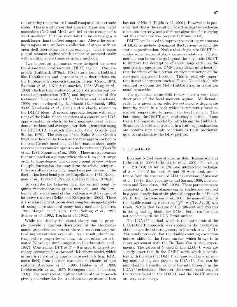
67

this ordering temperature is small compared to electronicscales. This is a situation that arises in transition metalmonoxides (NiO and MnO) and led to the concept of aMott insulator. In these materials the insulating gap ismuch larger than the Neel temperature. Above the order-ing temperature, we have a collection of atoms with anopen shell interacting via superexchange. This is againa local moment regime which cannot be accessed easilywith traditional electronic structure methods.

Two important approaches were designed to accessthe disordered local moment (DLM) regime. One ap-proach (Hubbard, 1979a,b, 1981) starts form a Hubbardlike Hamiltonian and introduces spin fluctuations viathe Hubbard–Stratonovich transformation (Cyrot, 1970;Evenson et al., 1970; Stratonovich, 1958; Wang et al.,1969) which is then evaluated using a static coherent po-tential approximation (CPA) and improvements of thistechnique. A dynamical CPA (Al-Attar and Kakehashi,1999) was developed by Kakehashi (Kakehashi, 1992,2002; Kakehashi et al., 1998) and is closely related tothe DMFT ideas. A second approach begins with solu-tions of the Kohn–Sham equations of a constrained LDAapproximation in which the local moments point in ran-dom directions, and averages over their orientation usingthe KKR–CPA approach (Faulkner, 1982; Gyorffy andStocks, 1979). The average of the Kohn–Sham Green’sfunctions then can be taken as the first approximation tothe true Green’s functions, and information about angleresolved photoemission spectra can be extracted (Gyorffyet al., 1985; Staunton et al., 1985). There are approachesthat are based on a picture where there is no short rangeorder to large degree. The opposite point of view, wherethe spin fluctuations far away form the critical tempera-ture are still relatively long ranged was put forward in thefluctuation local band picture (Capellmann, 1974; Koren-man et al., 1977a,b,c; Prange and Korenman, 1979a,b).

To describe the behavior near the critical point re-quires renormalization group methods, and the low–temperature treatment of this problem is still a subject ofintensive research (Belitz and Kirkpatrick, 2002). Thereis also a large literature on describing ferromagnetic met-als using more standard many–body methods (Liebsch,1981; Manghi et al., 1997, 1999; Nolting et al., 1987;Steiner et al., 1992; Treglia et al., 1982).

While the density functional theory can in princi-ple provide a rigorous description of the thermody-namic properties, at present there is no accurate prac-tical implementation available. As a result, the finite–temperature properties of magnetic materials are esti-mated following a simple suggestion (Liechtenstein et al.,1987). Constrained DFT at T = 0 is used to extract ex-change constants for a classical Heisenberg model, whichin turn is solved using approximate methods (e.g. RPA,mean–field) from classical statistical mechanics of spinsystems (Antropov et al., 1996; Halilov et al., 1998;Liechtenstein et al., 1987; Rosengaard and Johansson,1997). The most recent implementation of this approachgives good values for the transition temperature of Iron

but not of Nickel (Pajda et al., 2001). However it is pos-sible that this is the result of not extracting the exchangeconstants correctly, and a different algorithm for carryingout this procedure was proposed (Bruno, 2003).

DMFT can be used to improve the existing treatmentsof DLM to include dynamical fluctuations beyond thestatic approximation. Notice that single–site DMFT in-cludes some degree of short range correlations. Clustermethods can be used to go beyond the single–site DMFTto improve the description of short range order on thequasiparticle spectrum. DMFT also allows us to incorpo-rate the effects of the electron–electron interaction on theelectronic degrees of freedom. This is relatively impor-tant in metallic systems such as Fe and Ni and absolutelyessential to obtain the Mott–Hubbard gap in transitionmetal monoxides.

The dynamical mean–field theory offers a very cleardescription of the local moment regime. Mathemati-cally, it is given by an effective action of a degenerateimpurity model in a bath which is sufficiently weak ata given temperature to quench the local moment. Thisbath obeys the DMFT self–consistency condition. If onetreats the impurity model by introducing the Hubbard–Stratonovich field and treats it in a static approximation,one obtains very simple equations as those previouslyused to substantiate the DLM picture.

1. Iron and Nickel

Iron and Nickel were studied in Refs. Katsnelson andLichtenstein, 2000; Lichtenstein et al., 2001. The valuesU = 2.3 (3.0) eV for Fe (Ni) and interatomic exchangeof J = 0.9 eV for both Fe and Ni were used, as ob-tained from the constrained LDA calculations (Anisimovet al., 1997a; Bandyopadhyay and Sarma, 1989; Lichten-stein and Katsnelson, 1997, 1998). These parameters areconsistent with those of many earlier studies and resultedin a good description of the physical properties of Fe andNi. In Ref. Lichtenstein et al., 2001 the general form ofthe double counting correction V DC

σ = 12TrσMσ(0) was

taken. Notice that because of the different self–energiesin the eg and t2g blocks the DMFT Fermi surface doesnot coincide with the LDA Fermi surface.

The LDA+U method, which is the static limit of theLDA+DMFT approach, was applied to the calculationof the magnetic anisotropy energies (Imseok et al., 2001).This study revealed that the double counting correctioninduces shifts in the Fermi surface which brings it incloser agreement with the De Haas Van Alphen exper-iments. The values of U used in this LDA+U work areslightly lower than in the DMFT work, which is consis-tent with the idea that DMFT contains additional screen-ing mechanisms, not present in LDA+U. This can bemimicked by a smaller value of the interaction U in theLDA+U calculation. However, the overall consistency ofthe trends found in the LDA+U and the DMFT studiesare very satisfactory.

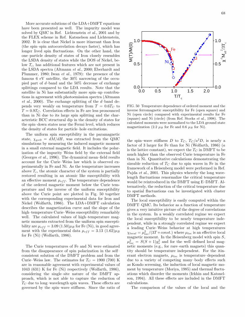
68

More accurate solutions of the LDA+DMFT equationshave been presented as well. The impurity model wassolved by QMC in Ref. Lichtenstein et al., 2001 and bythe FLEX scheme in Ref. Katsnelson and Lichtenstein,2002. It is clear that Nickel is more itinerant than Iron(the spin–spin autocorrelation decays faster), which haslonger lived spin fluctuations. On the other hand, theone–particle density of states of Iron closely resemblesthe LSDA density of states while the DOS of Nickel, be-low Tc, has additional features which are not present inthe LSDA spectra (Altmann et al., 2000; Eberhardt andPlummer, 1980; Iwan et al., 1979): the presence of thefamous 6 eV satellite, the 30% narrowing of the occu-pied part of d–band and the 50% decrease of exchangesplittings compared to the LDA results. Note that thesatellite in Ni has substantially more spin–up contribu-tions in agreement with photoemission spectra (Altmannet al., 2000). The exchange splitting of the d–band de-pends very weakly on temperature from T = 0.6TC toT = 0.9TC. Correlation effects in Fe are less pronouncedthan in Ni due to its large spin splitting and the char-acteristic BCC structural dip in the density of states forthe spin–down states near the Fermi level, which reducesthe density of states for particle–hole excitations.

The uniform spin susceptibility in the paramagneticstate, χq=0 = dM/dH , was extracted from the QMCsimulations by measuring the induced magnetic momentin a small external magnetic field. It includes the polar-ization of the impurity Weiss field by the external field(Georges et al., 1996). The dynamical mean–field resultsaccount for the Curie–Weiss law which is observed ex-perimentally in Fe and Ni. As the temperature increasesabove Tc, the atomic character of the system is partiallyrestored resulting in an atomic like susceptibility withan effective moment µeff . The temperature dependenceof the ordered magnetic moment below the Curie tem-perature and the inverse of the uniform susceptibilityabove the Curie point are plotted in Fig. 50 togetherwith the corresponding experimental data for Iron andNickel (Wolfarth, 1986). The LDA+DMFT calculationdescribes the magnetization curve and the slope of thehigh–temperature Curie–Weiss susceptibility remarkablywell. The calculated values of high–temperature mag-netic moments extracted from the uniform spin suscepti-bility are µeff = 3.09 (1.50)µB for Fe (Ni), in good agree-ment with the experimental data µeff = 3.13 (1.62)µB

for Fe (Ni) (Wolfarth, 1986).

The Curie temperatures of Fe and Ni were estimatedfrom the disappearance of spin polarization in the self–consistent solution of the DMFT problem and from theCurie–Weiss law. The estimates for TC = 1900 (700) Kare in reasonable agreement with experimental values of1043 (631) K for Fe (Ni) respectively (Wolfarth, 1986),considering the single–site nature of the DMFT ap-proach, which is not able to capture the reduction ofTC due to long–wavelength spin waves. These effects aregoverned by the spin–wave stiffness. Since the ratio of

0.0 0.5 1.0 1.5 2.00.0

0.5

1.0

0.0

0.5

1.0

Ni

Fe

χ-1M

eff2 /3

Tc

M(T

)/M

(0)

T/Tc

FIG. 50 Temperature dependence of ordered moment and theinverse ferromagnetic susceptibility for Fe (open square) andNi (open circle) compared with experimental results for Fe(square) and Ni (circle) (from Ref. Stocks et al., 1998). Thecalculated moments were normalized to the LDA ground statemagnetization (2.2 µB for Fe and 0.6 µB for Ni).

the spin–wave stiffness D to TC , TC/a2D, is nearly afactor of 3 larger for Fe than for Ni (Wolfarth, 1986) (ais the lattice constant), we expect the TC in DMFT to bemuch higher than the observed Curie temperature in Fethan in Ni. Quantitative calculations demonstrating thesizeable reduction of TC due to spin waves in Fe in theframework of a Heisenberg model were performed in Ref.Pajda et al., 2001. This physics whereby the long wave-length fluctuations renormalize the critical temperaturewould be reintroduced in the DMFT using E–DMFT. Al-ternatively, the reduction of the critical temperature dueto spatial fluctuations can be investigated with clusterDMFT methods.

The local susceptibility is easily computed within theDMFT–QMC. Its behavior as a function of temperaturegives a very intuitive picture of the degree of correlationsin the system. In a weakly correlated regime we expectthe local susceptibility to be nearly temperature inde-pendent, while in a strongly correlated regime we expecta leading Curie–Weiss behavior at high temperaturesχlocal = µ2

loc/(3T+const.) where µloc is an effective localmagnetic moment. In the Heisenberg model with spin S,µ2

loc = S(S + 1)g2s and for the well–defined local mag-

netic moments (e.g., for rare–earth magnets) this quan-tity should be temperature independent. For the itin-erant electron magnets, µloc is temperature–dependentdue to a variety of competing many–body effects suchas Kondo screening, the induction of local magnetic mo-ment by temperature (Moriya, 1985) and thermal fluctu-ations which disorder the moments (Irkhin and Katsnel-son, 1994). All these effects are included in the DMFTcalculations.

The comparison of the values of the local and the

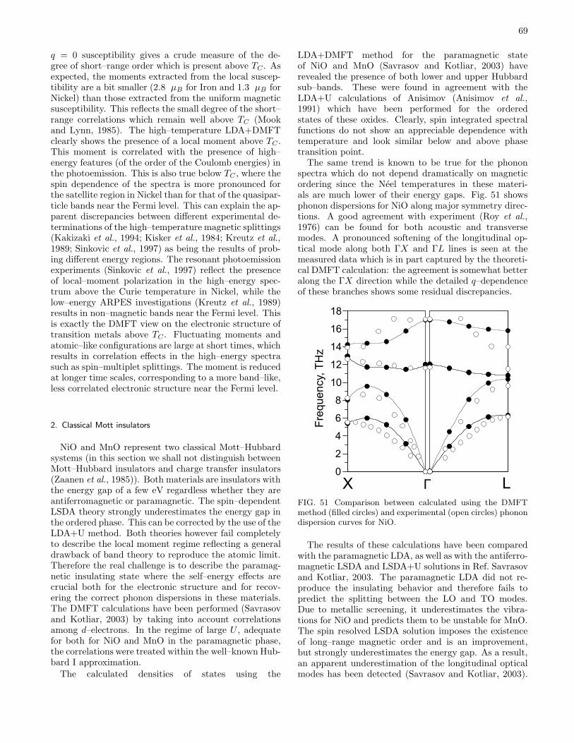
69

q = 0 susceptibility gives a crude measure of the de-gree of short–range order which is present above TC . Asexpected, the moments extracted from the local suscep-tibility are a bit smaller (2.8 µB for Iron and 1.3 µB forNickel) than those extracted from the uniform magneticsusceptibility. This reflects the small degree of the short–range correlations which remain well above TC (Mookand Lynn, 1985). The high–temperature LDA+DMFTclearly shows the presence of a local moment above TC .This moment is correlated with the presence of high–energy features (of the order of the Coulomb energies) inthe photoemission. This is also true below TC , where thespin dependence of the spectra is more pronounced forthe satellite region in Nickel than for that of the quasipar-ticle bands near the Fermi level. This can explain the ap-parent discrepancies between different experimental de-terminations of the high–temperature magnetic splittings(Kakizaki et al., 1994; Kisker et al., 1984; Kreutz et al.,1989; Sinkovic et al., 1997) as being the results of prob-ing different energy regions. The resonant photoemissionexperiments (Sinkovic et al., 1997) reflect the presenceof local–moment polarization in the high–energy spec-trum above the Curie temperature in Nickel, while thelow–energy ARPES investigations (Kreutz et al., 1989)results in non–magnetic bands near the Fermi level. Thisis exactly the DMFT view on the electronic structure oftransition metals above TC . Fluctuating moments andatomic–like configurations are large at short times, whichresults in correlation effects in the high–energy spectrasuch as spin–multiplet splittings. The moment is reducedat longer time scales, corresponding to a more band–like,less correlated electronic structure near the Fermi level.

2. Classical Mott insulators

NiO and MnO represent two classical Mott–Hubbardsystems (in this section we shall not distinguish betweenMott–Hubbard insulators and charge transfer insulators(Zaanen et al., 1985)). Both materials are insulators withthe energy gap of a few eV regardless whether they areantiferromagnetic or paramagnetic. The spin–dependentLSDA theory strongly underestimates the energy gap inthe ordered phase. This can be corrected by the use of theLDA+U method. Both theories however fail completelyto describe the local moment regime reflecting a generaldrawback of band theory to reproduce the atomic limit.Therefore the real challenge is to describe the paramag-netic insulating state where the self–energy effects arecrucial both for the electronic structure and for recov-ering the correct phonon dispersions in these materials.The DMFT calculations have been performed (Savrasovand Kotliar, 2003) by taking into account correlationsamong d–electrons. In the regime of large U , adequatefor both for NiO and MnO in the paramagnetic phase,the correlations were treated within the well–known Hub-bard I approximation.

The calculated densities of states using the

LDA+DMFT method for the paramagnetic stateof NiO and MnO (Savrasov and Kotliar, 2003) haverevealed the presence of both lower and upper Hubbardsub–bands. These were found in agreement with theLDA+U calculations of Anisimov (Anisimov et al.,1991) which have been performed for the orderedstates of these oxides. Clearly, spin integrated spectralfunctions do not show an appreciable dependence withtemperature and look similar below and above phasetransition point.

The same trend is known to be true for the phononspectra which do not depend dramatically on magneticordering since the Neel temperatures in these materi-als are much lower of their energy gaps. Fig. 51 showsphonon dispersions for NiO along major symmetry direc-tions. A good agreement with experiment (Roy et al.,1976) can be found for both acoustic and transversemodes. A pronounced softening of the longitudinal op-tical mode along both ΓX and ΓL lines is seen at themeasured data which is in part captured by the theoreti-cal DMFT calculation: the agreement is somewhat betteralong the ΓX direction while the detailed q–dependenceof these branches shows some residual discrepancies.

0

2

4

6

8

10

12

14

16

18F

req

ue

ncy,

TH

z

ΓX LFIG. 51 Comparison between calculated using the DMFTmethod (filled circles) and experimental (open circles) phonondispersion curves for NiO.

The results of these calculations have been comparedwith the paramagnetic LDA, as well as with the antiferro-magnetic LSDA and LSDA+U solutions in Ref. Savrasovand Kotliar, 2003. The paramagnetic LDA did not re-produce the insulating behavior and therefore fails topredict the splitting between the LO and TO modes.Due to metallic screening, it underestimates the vibra-tions for NiO and predicts them to be unstable for MnO.The spin resolved LSDA solution imposes the existenceof long–range magnetic order and is an improvement,but strongly underestimates the energy gap. As a result,an apparent underestimation of the longitudinal opticalmodes has been detected (Savrasov and Kotliar, 2003).

70

On the other hand, the calculations with correlations pro-duce much better results. This is found both for theLSDA+U and the LDA+Hubbard I calculations whichcan be interpreted as good approximations to the DMFTsolutions for the ordered and disordered magnetic states.Such an agreement can be related with the fact that thedirect d−d gap is fixed by U , and the charge transfer gapcomes out better in the theory. Thus, the local screeningof charge fluctuations are treated more appropriately.

D. Other applications

DMFT concepts and techniques are currently beingapplied to investigate a broad range of materials anda wide variety of strong correlation problems. This isa very active research frontier, comprising topics as di-verse as manganites, ruthenates, vanadates, actinides,lanthanides, Buckminster fullerenes, quantum criticalityin heavy fermion systems, magnetic semiconductors, ac-tinides, lanthanides, Bechgaard salts, high–temperaturesuperconductors, as well as surfaces heterostructures al-loys and many other types of materials. We mentionbelow a small subset of the systems under investiga-tion using the techniques described in this review, justin order to give the reader a glimpse of the breadth ofthis rapidly developing field and the great potential ofDMFT methods to investigate strongly correlated mate-rials. For earlier reviews see Ref. Held et al., 2001c andalso (Held et al., 2003), (Lichtenstein et al., 2002b) and(Georges, 2004a,b; Kotliar, 2005; Kotliar and Savrasov,2001; Kotliar and Vollhardt, 2004; Lichtenstein et al.,2002a).

Transition Metal Oxides• A large body of DMFT studies focused on the Mangan-ites with the perovskite structure, like La1−xCaxMnO3

or La1−xSrxMnO3. These materials attracted attentionbecause of their “colossal” magnetoresistance, which is anextreme sensitivity of resistance to an applied magneticfield (Dagotto, 2002; Tokura, 1990, 2003). The phasediagram of these materials in the temperature composi-tion plane is very rich, displaying ferromagnetism, anti-ferromagnetism, and charge and orbital ordering. Severalphysical mechanism and various interactions are impor-tant in these materials such as the double exchange mech-anism (i.e. the gain in kinetic energy of the eg electronswhen the t2g electrons are ferromagnetically aligned), thecoupling of the eg electrons to Jahn–Teller modes (i.e.distortions of the Oxygen octahedra which lift the cu-bic degeneracy of the eg orbitals) and breathing Oxy-gen phonon modes. These materials, as well as the cop-per oxides, also spurred new studies on strong electron-phonon coupling problems and their interplay with theelectron electron interactions. Semiclassical treatmentsof the core spins and the phonons, help to dramaticallysimplify the solution of the DMFT equations.

For various DMFT studies of the electron phonon cou-pling problem in the manganites see (Benedetti and Zey-

her, 1999; Blawid et al., 2003; Chernyshev and Fishman,2003; Ciuchi and De Pasquale, 1999; Ciuchi et al., 1997;Deppeler and Millis, 2002a,b; Fishman and Jarrell, 2002,2003a,b; Fratini et al., 2000, 2001; Furukawa, 1994; Heldand Vollhardt, 2000; Imai and Kawakami, 2000; Izyu-mov Yu and Letfulov, 2001; Michaelis and Millis, 2003;Millis et al., 1996b; Pankov et al., 2002; Phan and Tran,2003; Ramakrishnan et al., 2003, 2004; Tran, 2003; Ven-keteswara Pai et al., 2003).

• High-temperature superconductivity The discoveryof high-temperature superconductivity in the cupratesposed the great theoretical and computational challengeof uncovering the mechanism of this phenomena, whichis still not sufficiently understood to this day. The clus-ter extensions of DMFT are actively being applied inan effort to further unravel the mystery of the high-temperature superconductivity (Aryanpour et al., 2002;Civelli et al., 2005; Dahnken et al., 2004, 2005; Huscroftet al., 2001; Katsnelson and Lichtenstein, 2000; Macridinet al., 2004, 2005; Maier et al., 2000a, 2005, 2004b, 2002b;Potthoff et al., 2003).

• Other transition-metal oxides have recently beenstudied with DMFT. NaxCoO2 has received much inter-est due to anomalous thermoelectric properties in addi-tion to superconductivity upon hydration. (Ishida et al.,2005; Lechermann et al., 2005b; Saha-Dasgupta et al.,2005b). LiVO2 displays an unusually large effective massfor a d-electron system, which gave rise to the idea thatthis may be an example of a heavy-fermion d-electron ma-terial (Nekrasov et al., 2003). TiOCl displays 1d orbitalordering at low temperatures, and exhibits a spin-Peierlstransition (Hoinkis et al., 2005; Saha-Dasgupta et al.,2005a; Seidel et al., 2003). Ca2−xSrxRuO4 attracted alot of attention as it exhibits unconventional p–wave su-perconductivity at low temperatures, a Mott transition,and a surface-sensitive spectra (Anisimov et al., 2002;Lichtenstein and Liebsch, 2002; Liebsch, 2003a,b; Lieb-sch and Lichtenstein, 2000b).

Organic Materials and Supramolecular Struc-tures• Fullerines KnC 60. The doped Buckminster fullerenesare solids formed from C60 – a molecule shaped like asoccer ball – with the alkali metal sitting in the middle.Their proximity to the Mott transition was pointed outby Gunnarsson, 1997. At low temperatures K3C60 is ans–wave superconductor, where both the strong electron–phonon interaction and the Coulomb repulsion need tobe taken into account. DMFT has been helpful in under-standing the transition to superconductivity (Caponeet al., 2002a, 2000, 2002b; Han et al., 2003). A Mott in-sulating state has also been realized recently in anothernanostructured supercrystal family, that of potassiumloaded zeolites, and realistic DMFT calculations havebeen carried out (Arita et al., 2004).

• Bechgaard salts (Biermann et al., 2001; Vescoli et al.,2000). In addition to the quasi-two dimensional organiccompounds of the kappa and theta families mentionedin section IV, there have been chain-DMFT studies of

71

(TMTTF )2X and (TMTSF )2X . These are stronglyanisotropic materials made of stacks of organic molecules.Their optical properties are very unusual. At high tem-peratures the electrons move mainly along the chains, be-fore undergoing inelastic collisions forming a “Luttingerliquid” – one of the possible states of the one–dimensionalelectron gas. By contrast, at sufficiently low tempera-tures the electronic structure becomes effectively three–dimensional. For example, they exhibit a very narrowDrude peak carrying only one percent of the total opticalweight (Biermann et al., 2001; Vescoli et al., 2000). In-vestigations of the unusual properties of these materials,and in particular of the crossover between the low- andhigh–temperature regimes, using cluster generalizationsof DMFT have been performed in Refs. Biermann et al.,2001; Vescoli et al., 2000. Other aspects have recentlybeen addressed in Refs. Georges et al., 2000; Giamarchiet al., 2004.

Heavy Fermion Systems and Silicides• Heavy fermion materials are compounds containingboth f–electrons and lighter s, p, d–electrons. They canform a “heavy” Fermi liquid state at low temperatureswhere the quasiparticles are composites of f–electronspins and conduction electron charges, or can order anti-ferromagnetically at low temperatures (for recent reviewsee (Stewart, 2001)).

The boundary between the Fermi liquid and the itin-erant antiferromagnet has been a subject of intensivetheoretical and experimental study. Recent neutronscattering experiments are consistent with a local spinself–energy, and have motivated an extended dynami-cal mean–field descriptions of the Kondo lattice model(Si et. al. et al., 1999; Grempel and Si, 2003; Ingersentand Si, 2002; Jian-Xin et al., 2003; Si, 2001; Si et al.,2003, 2001) which reproduces many features of the ex-periment at zero temperature. For a recent discussionsee (Si, 2003). A corresponding study of Anderson lat-tice model (Sun and Kotliar, 2003) suggests that nonlo-cal effects, which require a cluster dynamical mean–fieldstudy, play an important role.

An interesting issue is whether the optical sum rule,integrated up to some cutoff of the order of one eV, canbe a strong function of temperature in heavy fermioninsulators. The f–sum rule states that if the integra-tion is performed up to infinite frequency, the result istemperature independent. In most materials, this sumrule is obeyed even when a finite upper limit of the or-der of an electronic energy is used. This was found inCe3Bi4Pt3 (Bucher et al., 1994) and in FeSi (Schlesingeret al., 1993)) (Smith et al., 2003; Urasaki and Saso, 2000;van der Marel, 2003). In Ref. Damascelli, 1999, ithas been shown that the integrated optical weight up to0.5 eV is a strong function of temperature, and if an insu-lating gap much smaller than the cutoff is open, spectralweight is transferred to very high frequencies. This prob-lem was theoretically addressed using single–site DMFTapplied to the Anderson lattice model, and the theorysupports a gradual filling of the gap without area conser-

vation (Rozenberg et al., 1995). More recent studies ap-plied to a multiband Hubbard model (Smith et al., 2003;Urasaki and Saso, 2000; van der Marel, 2003) and to theAnderson lattice (Vidhyadhiraja et al., 2003) yield excel-lent quantitative agreement with the most recent experi-ments. Of great interest is the behavior of these materialsin an external field, which is easily incorporated into theDMFT equations (de’ Medici et al., 2005b; Meyer andNolting, 2001).One interesting phenomena is the possibil-ity of metamagnetism, namely the anomalous increase ofthe magnetization and the concomitant changes in elec-tronic structure as a function of external field, known asa metamagnetic transition. This is displayed in manyheavy fermion systems such as CeRu2Si2. An importantissue is whether a transition between a state with a largeFermi surface and a small Fermi surface takes place as afunction of magnetic field.

Inhomogeneous Systems• Magnetic semiconductors are materials where the mag-netization is strongly tied to the carrier concentration.They offer the possibility of controlling the charge con-ductivity (as in the usual semiconductors) and the spinconductivity (by controlling the magnetization), by vary-ing the carrier concentration. Great excitement inthis field has been generated by the discovery of high–temperature ferromagnetism in these materials (Kubler,2000; Kuebler, 2002; Vollhardt et al., 1999). A mainchallenge is to understand the strong dependence of themagnetization on the carrier concentration of the mag-netic atoms and on the concentration of the conductionelectrons or holes. This problem is closely related tothe Anderson lattice model and several DMFT studiesof this problem have appeared (Chattopadhyay et al.,2001; Das Sarma et al., 2003). DMFT has been success-fully applied to half magnets such as NiMnSb (Chioncelet al., 2003a, 2005; Irkhin et al., 2004) as well as mag-netic multilayers (Chioncel and Lichtenstein, 2004). Fora recent DMFT study of the dependence of the criticaltemperature on various physical parameters see (Morenoet al., 2005).

• Strongly inhomogeneous systems: systems near anAnderson transition. The dynamical mean–field theoryhas been formulated to accommodate strongly inhomoge-neous situations such as systems near an Anderson tran-sition, by allowing an arbitrary site dependence of theWeiss field (Dobrosavljevic and Kotliar, 1997). Recentprogress in simplifying the analysis and solution of theseequations was achieved using the typical medium ap-proach of Dobrosavljevic et al. (Dobrosavljec et al., 2003).The statistical DMFT approach can also be used to studythe interplay of disorder and the electron–phonon cou-pling (Bronold and Fehske, 2003).

• Heterostructures surfaces and interfaces

Another application of DMFT is to study correlationeffects on surfaces, which likely to be more pronouncedthan in the bulk (Freericks, 2004; Okamoto and Millis,2004b,c,d). For an early discussion of these effects seeRefs. Hesper et al., 2000; Sawatzky, 1995. DMFT equa-

72

tions for the study of correlation effects on surfaces andsurfaces phase transitions were written down by Potthoffand collaborators (Potthoff and Nolting, 1999a,b,c). andsuccessfully applied to study the Mott transition on sur-faces by (Liebsch, 2003c; Perfetti et al., 2003). DMFThas been applied to inhomogeneous situations involvinga much longer periodicity. These studies were motivatedby the discovery of stripes in high–temperature super-conductors.

V. OUTLOOK

Dynamical mean–field methods represent a new ad-vance in many–body physics. They provide an excellentdescription of the strongly correlated regime of manythree–dimensional transition–metal oxides, which hadnot been accessible to other techniques. Additionally,DMFT has given new insights into strongly correlatedelectron systems near a metal–insulator transition, orlocalization–delocalization boundary.

The combination of advanced electronic structuremethods with the dynamical mean–field technique hasalready resulted in new powerful methods for modelingcorrelated materials. Further improvements are currentlybeing pursued, as the implementations of GW methodsand dynamical mean–field ideas (Aryasetiawan and Gun-narsson, 1998; Biermann et al., 2003; Sun and Kotliar,2002, 2004; Zein and Antropov, 2002).

In the field of statistical mechanics, the developmentof mean–field theories was followed up by the develop-ment of renormalization group approaches incorporatingthe physics of long wavelength fluctuations which becomedominant near critical points. The development of effec-tive renormalization techniques for correlated electronsand electronic structure applications is a major challengeahead. It will allow for more accurate derivation of low–energy Hamiltonians, and improve the solution of modelHamiltonians beyond the dynamical mean–field theorybased on small clusters.

The forces acting on the atoms have been recently eval-uated in the realistic DMFT treatment of phonons incorrelated electron systems (Dai et al., 2003; Savrasovand Kotliar, 2003). The indications that DMFT capturescorrectly the forces on the atoms in correlated materialsbodes well for combining this development with molec-ular dynamics to treat the motion of ions and electronssimultaneously. This remains one of the great challengesfor the future.

In conclusion, DMFT is a theory which can accuratelycapture local physics. We emphasize that the notionof local is flexible, and generically refers to some pre-defined region in which correlations are treated directly(e.g. a single–site, or a cluster of sites). Current com-putational limitations restrict the local region to be arelatively small number of sites for lattice models. De-spite this restriction, DMFT and its cluster extensionshave been very successful in describing a wide variety of

materials properties where conventional techniques suchas LDA have failed. Therefore, it seems that there finallyexists a general tool which can accurately treat many ofthe problems posed by strong correlation in realistic ma-terials. With the increasing number of realistic DMFTimplementations and studies of materials, more detailedcomparisons with experiments will emerge. Ultimately,this experience will allow us to understand which aspectsof the strong correlation problem lie within the scope ofthe method, and which aspects require the treatment ofnon–Gaussian, long wavelength fluctuations of collectivemodes not included in the approach.

Acknowledgments

The content of this review has been greatly influencedby numerous colleagues and collaborators, theorists andexperimentalists, that have lead to establish DynamicalMean Field Theory as a practical tool for the study of thephysical properties of strongly correlated materials. Par-ticular thanks go to the KITP, and to my coorganizers ofthe program on realistic studies of correlated materials,O. K Andersen, A. Georges and A. Lichtenstein, that cat-alyzed many efforts in the field including this review. Wethank E. Abrahams, A. Anisimov, V. Antropov, A. Arko,F. Aryasetiawan, S. Biermann, G. Biroli, C. Bolech, MCapone, C. Castellani, R. Chitra, M. Civelli, T.A. Costi,X. Dai, L. de Medici, S. Florens, T. Giamarchi, K. Held,D. Hess, M. Imada, J. Joyce, V. Kancharla, M. Katsnel-son, D. Koelling, A. Liebsch, W. Metzner, A. Migrliori,A. Millis, S. Murthy, G. Palsson, S. Pankov, I. Paul, A.Poteryaev, M. Rozenberg, A. Ruckenstein, S. Sachdev,P. Sun, J. Thompson, D. Vollhardt, J. Wong, N. Zein,and X.Y. Zhang.

The work at Rutgers (K. Haule, G. Kotliar , C.A.Marianetti, and V. Oudovenko ) was supported by anaward of the NSF-ITR program, under grant NSF-ITR-0312478. Gabriel Kotliar is a beneficiary of a ”ChaireInternationale de Recherche Blaise Pascal de l’Etat etde la Region d’Ille de France, geree par la Fondationde l’Ecole Normale Superieure”. O. Parcollet was sup-ported by the ACI of the French ministry of research.S. Savrasov acknowledges NSF DMR grants 0238188,0342290 and DOE Computational Material Science Net-work. The work was supported by the NSF DMR GrantsNo. 0096462, 02382188, 0312478, 0342290, US DOEdivision of Basic Energy Sciences Grant No DE-FG02-99ER45761, and by Los Alamos National Laboratorysubcontract No 44047-001-0237. Kavli Institute for The-oretical Physics is supported by NSF grant No. PHY99-07949.

73

APPENDIX A: Derivations for the QMC section

a. Derivation of Eq. (211) First, we show that

Trd†,d

∏

1≤k≤K

ed†A(k)d

= det

1 +

∏

1≤k≤K

eA(k)

(A1)where di (1 ≤ i ≤ n) are fermionic operators, A(k) (1 ≤k ≤ K) n × n matrices, and the notation d†A(k)d ≡∑

1≤i,j≤n d†iA

(k)ij dj . Indeed using

[d†Ad, d†Bd

]= d† [A,B] d (A2)

and Baker–Campbell–Hausdorff formula eAeB = eM

with

M ≡ A+B +1

2[A,B] + a2[A, [A,B]] + . . . (A3)

we have

exp(d†Ad) exp(d†Bd) = exp(d†Md)

By recursion, this generalizes to K matrices, so we justhave to prove the result for K = 1, A(1) = M . If M is di-agonal, the result is straightforward. For a general matrixM , by directly expanding the exponential of the left hand

side and using Wick theorem, we see that Trd†,ded†Md is

a series in TrMk (k ≥ 0) and is therefore invariant underany change of basis, and therefore det(1 + eM ). Hencethe result follows by diagonalizing M .

Second, we use the determinant formula

∣∣∣∣∣∣∣∣∣∣∣

1 0 . . . 0 BL

−B1 1 . . . . . . 0

0 −B2 1 . . . . . .

. . . . . . . . . 1 0

. . . . . . . . . −BL−1 1

∣∣∣∣∣∣∣∣∣∣∣

= det(1 +BLBL−1 . . . B1)

where B1, . . . , BL are n×nmatrices. This formula resultsby recursion from the general formula for block matrices:

det

(A B

C D

)= det

[(1 B

0 D

)(A−BD−1C 0

D−1C 1

)]

= detD det(A−BD−1C) (A4)

b. Derivation of Eq.(212) The first step is to obtain anexplicit formula for gS (Blankenbecler et al., 1981).

A quick way is to replace apµ and a†pν in the trace by

exp(ψ†Λ†µa) and exp(a†Λνψ), where ψ is an auxiliary

fermion and (Λµ)ij = λδj0δiµ where 0 is the index of ψ.Starting from the explicit trace expression of the Green’sfunction, distinguishing the cases l1 ≥ l2 and l1 < l2, us-ing Eq. (A1) and Eq. (A4), we finally expand to secondorder in λ and obtain (see also (Georges et al., 1996) ):

gσS(l1, l2) =

Bσ

l1−1 . . . Bσl2

(1 +Bσ

l2−1 . . . Bσ1B

σL . . . B

σl2

)−1for l1 ≥ l2

−Bσl1−1 . . . B

σ1B

σL . . . B

σl2

(1 +Bσ

l2−1 . . . Bσ1B

σL . . . B

σl2

)−1for l1 < l2

(A5)

A straightforward calculation then shows thatgσSOσ(S) = 1.

c. Derivation of Eq.(214) Equation (214) follows from the

observation that Oσ(S)∏1i=n e

−eViσ(S) depends onthe configuration S only on its diagonal blocks, whichleads to

Oσ(S)1∏

i=n

e−eViσ(S) −Oσ(S′)

1∏

i=n

e−eViσ(S′) =

1∏

i=n

e−eViσ(S) −

1∏

i=n

e−eViσ(S′) (A6)

which yields Eq. (214).

d. Derivation of the fast update formula (219) We presenthere the steps to go from Eq. (219) to Eq. (220). Sincethe difference between the two V is in the l block, Aσ

has the form

Aσ =

1 0 . . . Aσ1l . . . 0

0 1 . . . Aσ2l . . . 0

......

......

......

0 0 . . . Aσll . . . 0

......

......

......

0 0 . . . AσLl . . . 1

Using (A4), we have detAσ = detAσll. If detAσ

ll 6= 0, weuse the Woodbury formula where M is a N ×N matrixand U and V areN×P matrices (Golub and Loan, 1996):

(M +U tV )−1 = M−1 −M−1U(1 + tVM−1U

)−1tVM−1

74

with N = LN , P = N , M = 1, tU =(Ail

), tV =(

δil), 1 ≤ i ≤ L). to get

A−1σ =

1 0 . . . −Aσ1l(A

σll)

−1 . . . 0

0 1 . . . −Aσ2l(A

σll)

−1 . . . 0...

......

......

...

0 0 . . . (Aσll)

−1 . . . 0...

......

......

...

0 0 . . . −AσLl(A

σll)

−1 . . . 1

(A7)

which leads to Eq. (220).

APPENDIX B: Software for carrying out realistic DMFT

studies.

There is a growing interest to apply DMFT to real-istic models of strongly–correlated materials. In con-junction with this review, we provide a suite of DMFTcodes which implement some of the ideas outlined inthe review (http://dmftreview.rutgers.edu). These codesshould serve as a practical illustration of the method,in addition to lowering the barrier to newcomers in thefield who wish to apply DMFT. A strong effort was madeto isolate the various aspects of the DMFT calculationinto distinct subroutines and programs. This is a neces-sity both for conceptual clarity, and due to the fact thatvarious pieces of the code are under constant develop-ment. Additionally, we hope that this will increase theability of others to borrow different aspects of our codesand apply them in future codes or applications. Each ofthe codes performs some task or set of tasks outlined inthe LDA+DMFT flow chart (see Fig. 9) or the simplerDMFT flow chart (see Fig. 5).

a. Impurity solvers

DMFT is a mapping of a lattice problem onto an impu-rity problem. Therefore, at the heart of every DMFT cal-culation is the solution of the Anderson impurity model(section III). Solving the AIM is the most computation-ally demanding aspect of DMFT. No one solver is opti-mum for all of parameter space when considering both ac-curacy and computational cost. Therefore, we provide avariety of impurity solvers with this review. Additionally,more impurity solvers will be added to the webpage withtime, and existing impurity solvers will be generalized. Itshould be noted that some solvers are more general thanothers, and some of the solvers are already embeddedin codes which will perform DMFT on simple Hubbardmodels. The following solvers are currently available:QMC, FLEX, NCA, Hubbard I, and interpolative solver.(See sections III.D,III.A,III.B, III.C, and III.F, respec-tively.)

b. Density functional theory

Density functional theory (see section I.B.1) is the pri-mary tool used to study realistic materials, and in prac-tice it is usually the starting point for the study of re-alistic materials with strong correlations. Furthermore,current implementations of DMFT require the definitionof local orbitals. Therefore, DFT performed using anLMTO basis set is ideal match for DMFT. However, weshould emphasize that any basis set may be used (i.e.plane waves, etc) as long as local orbitals are defined.

Sergej Savrasov’s full–potential LMTO code (i.e. LM-TART) is provided to perform both DFT and DFT+U(i.e. LDA+U or GGA+U) calculations (see sections I.B.1and II.C, respectively). This code possesses a high degreeof automation, and only requires a few user inputs suchas the unit cell and the atomic species. The code out-puts a variety of quantities such as the total ground stateenergy, bands, density of states, optical properties, andreal–space hopping parameters. The code additionallycalculates forces, but no automatic relaxation scheme iscurrently implemented.

A Microsoft windows based graphical interface for LM-TART, Mindlab, is also provided. This allows an unfa-miliar user an intuitive interface to construct the inputfiles for LMTART, run LMTART, and analyze the resultsin a point–and–click environment. This code is especiallyhelpful for plotting and visualization of various resultsranging from the projected density of states to the Fermisurface.

c. DFT+DMFT

As stressed in this review, the ultimate goal of ourresearch is a fully first–principles electronic structuremethod which can treat strongly–correlated systems (i.e.see section I.B.3 II.E). Because this ambitious method-ology is still under development, we continue to rely onthe simplified approach which is DFT+DMFT (sectionI.B.1). Although simplified, DFT+DMFT is still techni-cally difficult to implement, and currently we only pro-vide codes which work within the atomic–sphere approx-imation (ASA) for the DFT portion of the calculation.One of the great merits of DFT+DMFT is that it is anearly first–principles method. The user only needs toinput the structure, the atomic species, and the inter-actions (i.e. U). The DFT+DMFT code suite is brokeninto three codes.

The first part is the DFT code, which is simply a mod-ified version of LMTART. It has nearly identical inputfiles, with minor differences in how the correlated or-bitals are specified. Therefore, the main inputs of thiscode are the unit cell and the atomic species. The mainrole of this code is to generate and export the convergedDFT Hamiltonian matrix in an orthogonalized local ba-sis for each k–point. Therefore, this code essentially gen-erates the parameters of the unperturbed Hamiltonian

75

automatically. This information is needed to constructthe local Green’s function.

The second part is the code which implements theDMFT self–consistency condition Eq. (121), which re-quires a choice of correlated orbitals. This code takesthe Hamiltonian matrix and the self–energy as input, andprovides the bath function as output.

The third part is the various codes which solve theAnderson impurity model, and these have been describedabove in the first section. These codes take the bathfunction as input and provide the self–energy, which isused in the self–consistency condition in the precedingstep.

These three pieces allow one to perform a non–self–consistent DFT+DMFT calculation as follows. First,the DFT code is used to generate the local, orthogo-nalized Hamiltonian matrix at each k–point. Second,one starts with a guess for the self–energy and usesthe DMFT self–consistency condition code to find thebath function. Third, the bath function is fed into theimpurity solver producing a new self–energy. The sec-ond and third steps are then repeated until DMFT self–consistency is achieved. This is considered a non–self–consistent DFT+DMFT calculation. In order to be fullyself– consistent, one should recompute the total densityafter DMFT self–consistency is achieved and use this asinput for the initial DFT calculation. This process shouldbe continued until both the total density and the localGreen’s function have converged. At the present time,we have not provided a routine to recompute the totaldensity following the self–consistent DMFT calculation,and therefore only non–self–consistent DFT+DMFT cal-culations are currently supported.

One should note that the above pieces which composethe DFT+DMFT suite are three separate codes. There-fore, one must write a simple script to iterate the abovealgorithm until self–consistency is reached (ie. the self-energy converges to within some tolerance). Addition-ally, the DFT portion of this code suite (i.e. the firstpart) can in principle be replaced by any DFT code aslong as a local basis set is generated.

d. Tight–binding cluster DMFT code (LISA)

The LISA (local Impurity Self-Consistent Approxima-tion) project is designed to provide a set of numericaltools to solve the quantum many-body problem of solidstate physics using Dynamical Mean Field Theory meth-ods (single site or clusters). The input to the programcan be either model Hamiltonians, or the output of otherab-initio calculations (in the form of tight binding pa-rameters and interaction matrices). This should greatlyfacilitate the development of realistic implementations ofdynamical mean field theory in electronic structure codesusing arbitrary basis sets.

This tool is provided to allow non-DMFT specialists tomake DMFT calculations with a reasonable investment.

However, DMFT methods are still in development andundergoing constant improvements. In particular, newimpurity solvers need to be developed and new clusterschemes will possibly be explored. Therefore numericaltools have to be flexible to accommodate foreseeable ex-tensions of the methods. In particular, one needs to beable to switch the solver easily while keeping the sameself-consistency condition. This can be achieved most ef-ficiently with modern programming techniques (e.g. ob-ject orientation, generic programming without sacrificingspeed since intensive parts of the program are quite lo-calized and can be easily optimized). These techniquesallow for a standardization of DMFT solvers by using anabstract solver class such that any new solver can be usedimmediately in various DMFT calculations. The use ofan abstract Lattice class allows for programs designed fortight-binding models like the Hubbard model to also beused for realistic calculations. A decomposition of theself-consistency conditions into small classes is beneficialin that various summation techniques on the Brillouinzone can be used or new cluster schemes can be tested.

With LISA, we hope to achieve flexible, reusable, andefficient software that is general enough to solve a varietyof models and to serve as a basis for future developments.Documentation, including examples, is provided with theweb page. At present, a library and a self–containedDMFT program are provided to solve a generalized tight–binding Hamiltonian with single–site or many variants ofcluster DMFT described in section II.B with the Hirsch-Fye QMC method. The tight–binding Hamiltonian maybe very simple, such as the traditional Hubbard modelor the p − d model of the cuprates, or very complex,such as a real material with longer range hoppings. Thisis markedly different than the DFT+DMFT code whichtakes the structure as input and generates the Hamilto-nian. The tight–binding Hamiltonian may be generatedby a variety of different electronic structure methods andcodes, or trivially specified in the case of a model Hamil-tonian.

APPENDIX C: Basics of the Baym–Kadanoff functional

The aim of these online notes is to provide a morepedagogical description of the use of functionals by usingthe Baym–Kadanoff functional as an example, and toderive, step–by–step, a few simple relations and formulaewhich are used in the main text.

In the Baym–Kadanoff theory, the observable of inter-est is the following operator

ψ†(x)ψ(x′), (C1)

and its average is the electron Green’s function G(x′, x) =−〈Tτψ(x′)ψ†(x)〉. As in the main text of the review weuse the notation x = (r, τ). The aim of the theory is toconstruct a functional that expresses the free energy ofthe system when the Green’s function is constrained tohave a given value.

76

First, we modify the action of the system so that itgives rise to the observable of our choice. This is achieved

by adding a source term to the action in the following way

e−F [J] =

∫D[ψ†ψ] exp

(−S −

∫dxdx′ψ†(x)J(x, x′)ψ(x′)

), (C2)

where the action S is given by S = S0 + λS1 where S0

is the free part of the action and S1 the interacting part.In electronic structure calculations

S1 =1

2λ

∫dxdx′ψ†(x)ψ†(x′)vC(x−x′)ψ(x′)ψ(x). (C3)

and vC is the Coulomb interaction.λ is a coupling constant that allows us to ”turn on”

the interaction. When λ = 0 we have a non interactingproblem and we have the interacting problem of interestwhen λ = 1.

The modified free energy Eq. (C2) is a functional ofthe source field J . F = F [J ]. By varying modified freeenergy Eq. (C2), F with respect to J we get

δF [J, λ]

δJ= G, (C4)

The solution of this equation, gives J = J(λ,G).Its meaning is the source that results for a given

Green’s function G when the interaction is λ. Noticethat when λ is set to unity and G is the true Greensfunction of the original problem (i.e. J = 0, λ = 1 ) Jvanishes by definition.

When G is the true Greens function of the originalproblem and λ = 0, J(λ = 0, G) is non–zero and is equalto the interacting self–energy Σint. This is because theinteracting self–energy is the quantity that needs to beadded to the non–interacting action to get the interactingGreen’s function. We will show how this works mathe-matically below.

We now make a Legendre transform from source theJ to Green’s function G, to get a functional of Green’sfunction only

ΓBK [G, λ] = F [J [λ,G], λ] − Tr[JG] (C5)

with the differential

δΓBK = −Tr[J δG]. (C6)

ΓBK [G] is the functional which, as we will show be-low, gives the free–energy and the Greens function of theinteracting system at its saddle point. It is very usefulfor constructing numerous approximations. The Legen-dre transform is used extensively in statistical mechan-ics, and the above procedure parallels transforming fromthe canonical to the grand–canonical ensemble where thechemical potential replaces the density as the indepen-dent variable.

Now we want to connect the solution of the interact-ing system λ = 1 with the corresponding non–interactingλ = 0 problem and split functional ΓBK [G] into the sim-ple non–interacting part and a more complicated inter-acting part.

1. Baym–Kadanoff functional at λ = 0

If λ is set to zero, the functional integral (C2) canreadily be computed

e−F0[J0] =

∫D[ψ†ψ] exp

(−∫dxdx′ψ†(x)(

∂

∂τ− µ+H0 + J0)ψ(x′)

)= Det(

∂

∂τ− µ+H0 + J0), (C7)

and the free energy becomes

F0[J0] = −Tr ln(G−1

0 − J0

), (C8)

where we neglected a constant term Tr ln(−1). Here J0 isJ(λ = 0) and F0 is F (λ = 0), while G0 = (ω+µ−H0)

−1

is the usual non–interacting Green’s function. Taking

into account Eq. (C4), the Green’s function at λ = 0 is

G =δF0[J0]

δJ0=(G−1

0 − J0

)−1. (C9)

Since the Green’s function G is fixed at the interactingGreen’s function, it is clear that the source field J0 isthe interacting self–energy, viewed as a function of the

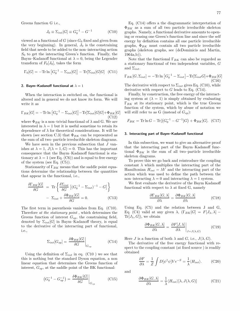
77

Greens function G i.e.,

J0 ≡ Σint[G] ≡ G−10 −G−1 (C10)

viewed as a functional ofG (sinceG0 fixed and given fromthe very beginning). In general, J0 is the constrainingfield that needs to be added to the non–interacting actionS0 to get the interacting Green’s function. Finally, theBaym–Kadanoff functional at λ = 0, being the Legendretransform of F0[J0], takes the form

Γ0[G] = −Tr ln[G−1

0 − Σint[G]]− Tr[Σint[G]G] (C11)

2. Baym–Kadanoff functional at λ = 1

When the interaction is switched on, the functional isaltered and in general we do not know its form. We willwrite it as

ΓBK [G] = −Tr ln[G−1

0 − Σint[G]]−Tr[Σint[G]G]+ΦBK [G]

(C12)where ΦBK is a non–trivial functional of λ and G. We areinterested in λ = 1 but it is useful sometime to retain itsdependence of λ for theoretical considerations. It will beshown (see section C.3) that ΦBK can be represented asthe sum of all two–particle irreducible skeleton diagrams.

We have seen in the previous subsection that J van-ishes at λ = 1, J(λ = 1, G) = 0. This has the importantconsequence that the Baym–Kadanoff functional is sta-tionary at λ = 1 (see Eq. (C6)) and is equal to free energyof the system (see Eq. (C5)).

Stationarity of ΓBK means that the saddle point equa-tions determine the relationship between the quantitiesthat appear in the functional, i.e.,

δΓBK [G]

δG= Tr

δΣint

δG

[(G−1

0 − Σint)−1 −G

]

− Σint +δΦBK [G]

δG= 0. (C13)

The first term in parenthesis vanishes from Eq. (C10).Therefore at the stationary point , which determines theGreens function of interest Gsp, the constraining field,denoted by Σint[G] in Baym–Kadanoff theory, is equalto the derivative of the interacting part of functional,i.e.,

Σint[Gsp] =δΦBK [G]

δG

∣∣∣∣Gsp

(C14)

Using the definition of Σint in eq. (C10 ) we see thatthis is nothing but the standard Dyson equation, a nonlinear equation that determines the Greens function ofinterest, Gsp, at the saddle point of the BK functional:

(G−1

0 −G−1sp

)=δΦBK [G]

δG

∣∣∣∣Gsp

(C15)

Eq. (C14) offers a the diagrammatic interpretation ofΦBK as a sum of all two particle irreducible skeletongraphs. Namely, a functional derivative amounts to open-ing or erasing one Green’s function line and since the selfenergy by definition contains all one particle irreduciblegraphs, ΦBK must contain all two particle irreduciblegraphs (skeleton graphs, see (deDominicis and Martin,1964a,b)).

Note that the functional ΓBK can also be regarded asa stationary functional of two independent variables, Gand Σint.

ΓBK [G,Σint] = −Tr ln[G−1

0 − Σint

]−Tr[ΣintG]+ΦBK [G]

(C16)The derivative with respect to Σint gives Eq. (C10), whilederivative with respect to G leads to Eq. (C14).

Finally, by construction, the free energy of the interact-ing system at (λ = 1) is simply obtained by evaluatingΓBK at its stationary point, which is the true Greensfunction of the system, which by abuse of notation wewill still refer to as G (instead of Gsp):

FBK = Tr lnG− Tr[(G−1

0 −G−1]G)

+ ΦBK [G]. (C17)

3. Interacting part of Baym–Kadanoff functional

In this subsection, we want to give an alternative proofthat the interacting part of the Baym–Kadanoff func-tional ΦBK is the sum of all two–particle irreducibleskeleton diagrams.

To prove this we go back and reintroduce the couplingconstant λ which multiplies the interacting part of theHamiltonian Hint = λV and the interacting part of theaction which was used to define the path between thenon–interacting λ = 0 and interacting λ = 1 system.

We first evaluate the derivative of the Baym Kadanofffunctional with respect to λ at fixed G, namely

∂ΓBK [G, λ]

∂λ=∂ΦBK [G, λ]

∂λ(C18)

Using Eq. (C5) and the relation between J and G,Eq. (C4) valid at any given λ, (ΓBK [G] = F [Jλ, λ] −Tr[Jλ, G]), we obtain

∂ΦBK [G, λ]

∂λ=

∂F [J, λ]

∂λ

∣∣∣∣J=J(λ,G)

(C19)

Here J is a function of both λ and G, i.e., J(λ,G).The derivative of the free energy functional with re-

spect to the coupling constant (at fixed source ) is readilyobtained

∂F

∂λ=

1

Z

∫D[ψ†ψ]V e−S =

1

λ〈Hint〉. (C20)

and

∂ΦBK [G, λ]

∂λ=

1

λ〈Hint〉[λ, J(λ,G)] (C21)

78

Notice that Hint or S1 is independent of of J, but theaverage 〈 〉 is carried out with respect to a weight whichcontains the source explicitly. Integrating equation (C21):

ΦBK [G] =

∫

0

1 1

λ〈Hint〉[λ, J(λ,G)]dλ (C22)

This is another example of the coupling constant in-tegration formula for the interaction energy of the ef-fective actions constructed in our review. Equation(C22) can be expanded in a standard perturbation the-ory. We take as the inverse unperturbed propagatorG0

−1−J(λ = 0) ( namely G ) and as interaction verticesHint and [J(λ) − J(λ = 0)]ψ†ψ as interaction vertices.This means that the perturbation theory contains twokinds of vertices , the first carries 4 legs and the seconddenoted by a cross carries only two legs and represents[J(λ) − J(λ = 0)]ψ†ψ. The role of the second vertex isto eliminate the graphs which are two particle reducible,this cancellation is illustrated in figure 52. which demon-strates that for each reducible graph (i.e. one having aself energy insertion ), there is also a cross, their sum iszero as a result of the equation

J [λ] − J [λ = 0] + Σ[λ] = 0 (C23)

This equation is proved by noticing that at a givenvalue of λ the Greens function of the problem is by defini-

tion G0−1 − J(λ = 0) − Σ[λ]

−1= G and since by defini-

tion G0−1 − J(λ = 0)

−1= G combining these two equa-

tions we obtain Eq. (C23). The role of the coupling

= 0+

FIG. 52 Mechanism of cancellation of reducible graphs. The”X” denotes J(λ) − J(λ = 0) and the circles in blue are theself-energy insertions that make the graph reducible.

constant integration is to provide the standard symme-try factors in the free energy graphs.

4. The total energy

In this subsection, we want to derive the relationshipbetween the total energy of the system and the corre-sponding Green’s function. Let us start by the definition

of the Green’s function

G(x1, x2) = −〈Tτψ(x1)ψ†(x2)〉. (C24)

The non–interacting (quadratic) part of the Hamiltonian

βH0 =

∫dx1dx2ψ

†(x1)H0x1x2δ(τ1 − τ2)ψ(x2), (C25)

can be expressed by the Green’s function in the followingway

β〈H0〉 =

∫dx1dx2H0x1x2δ(τ1 − τ2)〈ψ†(x1)ψ(x2)〉(C26)

=

∫dx1dx2H0x1x2G(x2, x1)δ(τ2 − τ1 + 0+).(C27)

To get the interacting part of the total energy, we aregoing to examine the time derivative of the Green’s func-tion which follows directly from the definition Eq. (C24)and takes the form(∂G(x1, x2)

∂τ1

)

τ1 → τ2 − 0+

r1 → r2

= 〈ψ†(x1) [H − µn, ψ(x1)]〉. (C28)

The resulting commutator can be simplified by notingthat the following two commutators take a very simpleform

∫dxψ†(x) [ψ(x), V ] = 2V (C29)

∫dxψ†(x) [ψ(x), H0] = H0. (C30)

where V is the normal–ordered electron–electron interac-tion. The factor two in the above equation follows fromthe fact that the interaction term is quartic in ψ whileH0 is quadratic.

It is more convenient to express the equations in imagi-nary frequency than the imaginary time. Using the trans-formation

G(x1, x2) = T∑

iω

e−iω(τ1−τ2)Giω(r1, r2), (C31)

one obtains for the non–interacting part

T

∫dr1dr2H0r1r2

∑

iω

Giω(r2, r1)eiω0+

= 〈H0〉, (C32)

while the time derivative from Eq. (C28) gives

T

∫dr1

∑

iω

(iω)eiω0+

Giω(r1, r1) = 〈H0 + 2V − µn〉.

(C33)Combining equations (C32) and (C33) leads to the fol-lowing expression for the interaction energy

79

〈V 〉 =1

2T

∫dr1dr2

∑

iω

eiω0+ [(iω + µ)δ(r1 − r2) −H0r1r2 ]Giω(r2, r1) =1

2Tr[eiω0+ G−1

0 G] =1

2Tr[ΣG]. (C34)

Here we took into account that∑

iω eiω0+ = 0. Finally, the total energy becomes

〈H〉 =1

2T

∫dr1dr2

∑

iω

eiω0+ [(iω + µ)δ(r1 − r2) +H0r1r2 ]Giω(r2, r1) = Tr[H0G+1

2ΣG]. (C35)

References

Abrikosov, A. A., 1965, Physica 2, 21.Si et. al., S., J. L. Smith, and K. Ingersent, 1999, Int. J. Mod.

Phys. B 13, 2331.Al-Attar, H., and Y. Kakehashi, 1999, J. Appl. Phys. 86,

3265.Allen, J. W., and L. Z. Liu, 1992, Phys. Rev. B 46, 5047.Allen, J. W., and R. M. Martin, 1982, Phys. Rev. Lett. 49,

1106.Almbladh, C. O., U. Von Barth, and R. Van Leeuwen, 1999,

Int. J. Mod. Phys. B 13, 535.Altmann, K. N., D. Y. Petrovykh, G. J. Mankey, N. Shan-

non, N. Gilman, M. Hochstrasser, R. F. Willis, and F. J.Himpsel, 2000, Phys. Rev. B 61, 15661.

Amadon, B., S. Biermann, and A. G. andF. Aryasetiawan,2005, Electronic archive, xxx.lanl.gov, cond-mat/0504732 .

Andersen, O. K., 1975, Phys. Rev. B 12, 3060.Andersen, O. K., and O. Jepsen, 1984, Phys. Rev. Lett. 53,

2571.Anderson, P. W., 1961, Phys. Rev. 124, 41.Anisimov, V., A. Poteryaev, M. Korotin, A. Anokhin, and

G. Kotliar, 1997a, J. Phys.: Condens. Matter 9, 7359.Anisimov, V. I., F. Aryasetiawan, and A. I. Lichtenstein,

1997b, J. Phys.: Condens. Matter 9, 767.Anisimov, V. I., and O. Gunnarsson, 1991, Phys. Rev. B 43,

7570.Anisimov, V. I., I. A. Nekrasov, D. E. Kondakov, T. M. Rice,

and M. Sigrist, 2002, Eur. Phys. J. B 25, 191.Anisimov, V. I., J. Zaanen, and O. K. Andersen, 1991, Phys.

Rev. B 44, 943.Antropov, V. P., M. I. Katsnelson, B. N. Harmon, M. van

Schilfgaarde, and D. Kusnezov, 1996, Phys. Rev. B 54,1019.

Argaman, N., and G. Makov, 2000, Am. J. Phys. 68, 69.Arita, R., and K. Held, 2005, Electronic archive, xxx.lanl.gov,

cond-mat/0504040 .Arita, R., T. Miyake, T. Kotani, M. van Schilfgaarde, T. Oka,

K. Kuroki, Y. Nozue, and H. Aoki, 2004, Phys. Rev. B 69,195106.

Arko, A. J., J. J. Joyce, L. Morales, J. Wills, J. Lashley,F. Wastin, and J. Rebizant, 2000, Phys. Rev. B 62, 1773.

Arnaud, B., and M. Alouani, 2000, Phys. Rev. B 62, 4464.Aryanpour, K., M. H. Hettler, and M. Jarrell, 2002, Phys.

Rev. B 65, 153102.Aryanpour, K., T. Maier, and M. Jarrell, 2005, Phys. Rev. B

71, 037101.Aryasetiawan, F., S. Biermann, and A. Georges, 2004a, Elec-

tronic archive, xxx.lanl.gov, cond-mat/0401626 .Aryasetiawan, F., and O. Gunnarsson, 1998, Rep. Prog. Phys.

61, 237.Aryasetiawan, F., M. Imada, A. Georges, G. Kotliar, S. Bier-

mann, and A. I. Lichtenstein, 2004b, Phys. Rev. B 70,195104.

Bandyopadhyay, M. T., and D. D. Sarma, 1989, Phys. Rev.B 39, 3517.

Barnes, S. E., 1976, J. Phys. F 6, 1375.Barnes, S. E., 1977, J. Phys. F 7, 2637.Baroni, S., P. Gainnozzi, and A. Testa, 1987, Phys. Rev. Lett.

58, 1861.Baroni, S., S. de Gironcoli, A. D. Corso, and P. Giannozzi,

2001, Rev. Mod. Phys. 73, 515.von Barth, U., and L. Hedin, 1972, J. Phys. C 5, 1629.Baym, G., 1962, Phys. Rev. 127, 1391.Baym, G., and L. P. Kadanoff, 1961, Phys. Rev. 124, 287.Belitz, D., and T. R. Kirkpatrick, 2002, Phys. Rev. Lett. 89,

247202.Benedetti, P., and R. Zeyher, 1999, Phys. Rev. B 59, 9923.Bickers, N. E., and D. J. Scalapino, 1989, Ann. Phys. (N.Y.)

193, 206.Bickers, N. E., and S. R. White, 1991, Phys. Rev. B 43, 8044.Biermann, S., F. Aryasetiawan, and A. Georges, 2003, Phys.

Rev. Lett. 90, 086402.Biermann, S., F. Aryasetiawan, and A. Georges, 2004, Elec-

tronic archive, xxx.lanl.gov, cond-mat/0401653 .Biermann, S., L. de’ Medici, and A. Georges, 2005a, Elec-

tronic archive, xxx.lanl.gov, cond-mat/0505737 .Biermann, S., A. Georges, A. Lichtenstein, and T. Giamarchi,

2001, Phys. Rev. Lett. 87, 276405.Biermann, S., A. Poteryaev, A. I. Lichtenstein, and

A. Georges, 2005b, Phys. Rev. Lett. 94, 026404.Biroli, G., and G. Kotliar, 2002, Phys. Rev. B 65, 155112.Biroli, G., and G. Kotliar, 2004, Electronic archive,

xxx.lanl.gov, cond-mat/0404537 .Biroli, G., and G. Kotliar, 2005, Phys. Rev. B 71, 037102.Biroli, G., O. Parcollet, and G. Kotliar, 2004, Phys. Rev. B

69, 205108.Blankenbecler, R., D. J. Scalapino, and R. L. Sugar, 1981,

Phys. Rev. D 24, 2278.Blawid, S., A. Deppeler, and A. J. Millis, 2003, Phys. Rev. B

67, 165105.Bloechl, P., 1989, Total Energies, Forces and Metal-

Semiconductor Interfaces, Ph.D. thesis, Max-Planck Instu-ture fur Festkoeperforschung, Stuttgart, Germany.

Bohm, D., and D. Pines, 1951, Phys. Rev. 82, 625.Bohm, D., and D. Pines, 1952, Phys. Rev. 85, 338.Bohm, D., and D. Pines, 1953, Phys. Rev. 92, 609.Bolech, C. J., S. S. Kancharla, and G. Kotliar, 2003, Phys.

Rev. B 67, 75110.Bonca, J., and J. E. Gubernatis, 1993, Phys. Rev. B 47,

80

13137.Boring, A. M., and J. L. Smith, 2000, Los Alamos Science 26,

91.Bouchet, J., B. Siberchicot, F. Jollet, and A. Pasturel, 2000,

J. Phys.: Condens. Matter 12, 1723.Bray, A. J., and M. A. Moore, 1980, J. Phys. C 13(24), L655.Bronold, F. X., and H. Fehske, 2003, Inst. Phys. Jagellonian

Univ. Acta Physica Polonica B 34, 851.Bruno, P., 2003, Phys. Rev. Lett. 90, 087205.Bucher, B., Z. Schlesinger, P. C. Canfield, and Z. Fisk, 1994,

Phys. Rev. Lett. 72, 522.Bulut, N., D. Scalapino, and S. White, 1993, Phys. Rev. B

47, 2742.Bunemann, J., F. Gebhard, T. Ohm, R. Umstatter, S. Weiser,

W. Weber, R. Claessen, D. Ehm, A. Harasawa, A. Kakizak,A. Kimura, G. Nicolay, et al., 2003, Europhys. Lett. 61,667.

Bunemann, J., and W. Weber, 1997, Phys. Rev. B 55, 4011.Bunemann, J., W. Weber, and F. Gebhard, 1998, Phys. Rev.

B 57, 6896.C. Knecht and N. Blumer and P. G. J. van Dongen, 2005,

Electronic archive, xxx.lanl.gov, cond-mat/0505106 .Caffarel, M., and W. Krauth, 1994, Phys. Rev. Lett. 72, 1545.Capellmann, H., 1974, J. Phys. F: Met. Phys. 4, 1466.Capone, M., M. Civelli, S. S. Kancharla, C. Castellani, and

G. Kotliar, 2004, Phys. Rev. B 69, 195105.Capone, M., M. Fabrizio, C. Castellani, and E. Tosatti, 2002a,

Science 296, 2364.Capone, M., M. Fabrizio, P. Giannozzi, and E. Tosatti, 2000,

Phys. Rev. B 62, 7619.Capone, M., M. Fabrizio, and E. Tosatti, 2002b, J. Phys.

Chem. Solids 63, 1555.Castellani, C., C. Di Castro, D. Feinberg, and J. Ranninger,

1979, Phys. Rev. Lett. 43, 1957.Castellani, C., G. Kotliar, R. Raimondi, M. Grilli, Z. Wang,

and M. Rozenberg, 1992, Phys. Rev. Lett. 69, 2009.Castellani, C., C. R. Natoli, and J. Ranninger, 1978a, Phys.

Rev. B 18, 4945.Castellani, C., C. R. Natoli, and J. Ranninger, 1978b, Phys.

Rev. B 18, 5001.Ceperley, D. M., and B. J. Alder, 1980, Phys. Rev. Lett. 45,

566.Chattopadhyay, A., S. Das Sarma, and A. J. Millis, 2001,

Phys. Rev. Lett. 87, 227202.Chernyshev, A. L., and R. S. Fishman, 2003, Phys. Rev. Lett.

90, 177202.Chioncel, L., M. I. Katsnelson, R. A. de Groot, and A. I.

Lichtenstein, 2003a, Phys. Rev. B 68, 144425.Chioncel, L., M. I. Katsnelson, G. A. de Wijs, R. A. de Groot,

and A. I. Lichtenstein, 2005, Phys. Rev. B 71, 85111.Chioncel, L., and A. I. Lichtenstein, 2004, Electronic archive,

xxx.lanl.gov, cond-mat/0403685 .Chioncel, L., L. Vitos, I. A. Abrikosov, J. Kollar, M. I. Kat-

snelson, and A. I. Lichtenstein, 2003b, Phys. Rev. B 67,235106.

Chioncel, L., L. Vitos, I. A. Abrikosov, J. Kollar, M. I. Kat-snelson, and A. I. Lichtenstein, 2003c, Phys. Rev. B 67,235106.

Chitra, R., and G. Kotliar, 1999, Phys. Rev. Lett. 83, 2386.Chitra, R., and G. Kotliar, 2000a, Phys. Rev. B 62, 12715.Chitra, R., and G. Kotliar, 2000b, Phys. Rev. Lett. 84, 3678.Chitra, R., and G. Kotliar, 2001, Phys. Rev. B 63, 115110.Ciuchi, S., and F. De Pasquale, 1999, Phys. Rev. B 59, 5431.Ciuchi, S., F. de Pasquale, S. Fratini, and D. Feinberg, 1997,

Phys. Rev. B 56, 4494.Civelli, M., M. Capone, S. S. Kancharla, O. Parcollet, and

G. Kotliar, 2005, Phys. Rev. Lett. 95, 106402.Coleman, P., 1984, Phys. Rev. B 29, 3035.Cornwall, J. M., R. Jackiw, and E. Tomboulis, 1974, Phys.

Rev. D 10, 2428.Costi, T. A., 1986, J. Phys. C 19, 5665.Costi, T. A., J. Kroha, and P. Wolfle, 1996, Phys. Rev. B 53,

1850.Cox, D. L., and A. E. Ruckenstein, 1993, Phys. Rev. Lett. 71,

1613.Craco, L., M. Laad, and E. Muller-Hartmann, 2003a, Phys.

Rev. B 68, 233310.Craco, L., M. Laad, and E. Muller-Hartmann, 2003b, Phys.

Rev. Lett. 90, 237203.Crandles, D. A., T. Timusk, J. D. Garrett, and J. E. Greedan,

1992, Physica C 201, 407.Cyrot, M., 1970, Phys. Rev. Lett. 25, 871.Dagotto, E., 1994, Rev. Mod. Phys. 66, 763.Dagotto, E., 2002, Nanoscale Phase Separation and Colossal

Magnetoresistance : The Physics of Manganites and Re-

lated Compounds (Springer-Verlag, Berlin, Germany).Dahnken, C., M. Aichhorn, W. Hanke, E. Arrigoni, and

M. Potthoff, 2004, Physical Review B-Condensed Matter70, 245110.

Dahnken, C., E. Arrigoni, and W. Hanke, 2002, J. Low Temp.Phys. 126, 949.

Dahnken, C., M. Potthoff, E. Arrigoni, and W. Hanke, 2005,Electronic archive, xxx.lanl.gov, cond-mat/0504618 .

Dai, X., K. Haule, and G. Kotliar, 2005, Phys. Rev. B 72,045111.

Dai, X., S. Y. Savrasov, G. Kotliar, A. Migliori, H. Ledbetter,and E. Abrahams, 2003, Science 300, 953.

Damascelli, A., 1999,http://www.ub.rug.nl/eldoc/dis/science/a.damascelli/ .

Das Sarma, S., E. H. Hwang, and A. Kaminski, 2003, Phys.Rev. B 67, 155201.

de’ Medici, L., A. Georges, and S. Biermann, 2005a, Elec-tronic archive, xxx.lanl.gov, cond-mat/0503764 .

de’ Medici, L., A. Georges, G. Kotliar, and S. Biermann,2005b, Electronic archive, xxx.lanl.gov, cond-mat/0502563.

Dederichs, P. H., S. Blugel, R. Zeller, and H. Akai, 1984, Phys.Rev. Lett. 53, 2512.

deDominicis, C., and P. Martin, 1964a, J. Math. Phys. 5, 14.deDominicis, C., and P. Martin, 1964b, J. Math. Phys. 5, 31.Deppeler, A., and A. J. Millis, 2002a, Phys. Rev. B 65,

224301.Deppeler, A., and A. J. Millis, 2002b, Phys. Rev. B 65,

100301.Desclaux, J. P., and A. J. Freeman, 1984, in Handbook on the

Physics and Chemistry of the Actinides, edited by A. J.Freeman and G. H. Lander (Elsevier, Amsterdam), vol-ume 1, p. 46.

Dobrosavljec, V., A. A. Pastor, and B. K. Nikolic, 2003, Eu-rophys. Lett. 62, 76.

Dobrosavljevic, V., and G. Kotliar, 1997, Phys. Rev. Lett. 78,3943.

Dobson, J. F., G. Vignale, and M. P. Das (eds.), 1997, Elec-

tronic Density Functional Theory: Recent Progress and

New Directions (Plenum, New York).Drchal, V., V. Janis, and J. Kudrnovsky, 1999, Phys. Rev. B

60, 15664.Drchal, V., V. Janis, J. Kudrnovsky, V. S. Oudovenko, X. Dai,

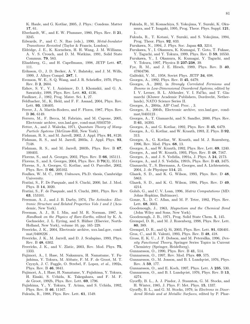
81

K. Haule, and G. Kotliar, 2005, J. Phys.: Condens. Matter17, 61.

Eberhardt, W., and E. W. Plummer, 1980, Phys. Rev. B 21,3245.

Edwards, P., and C. N. Rao (eds.), 1990, Metal-Insulator

Transitions Revisited (Taylor & Francis, London).Eldridge, J. E., K. Kornelsen, H. H. Wang, J. M. Williams,

A. V. S. Crouch, and D. M. Watkins, 1991, Solid StateCommun. 79, 583.

Eliashberg, G., and H. Capellmann, 1998, JETP Lett. 67,111.

Eriksson, O., J. D. Becker, A. V. Balatsky, and J. M. Wills,1999, J. Alloys Compd. 287, 1.

Evenson, W. E., S. Q. Wang, and J. R. Schrieffer, 1970, Phys.Rev. B 2, 2604.

Ezhov, S. Y., V. I. Anisimov, D. I. Khomskii, and G. A.Sawatzky, 1999, Phys. Rev. Lett. 83, 4136.

Faulkner, J., 1982, Prog. Mater. Sci. 1, 27.Feldbacher, M., K. Held, and F. F. Assaad, 2004, Phys. Rev.

Lett. 93, 136405.Ferrer, J., A. Martın-Rodero, and F. Flores, 1987, Phys. Rev.

B 36, 6149.Ferrero, M., F. Becca, M. Fabrizio, and M. Capone, 2005,

Electronic archive, xxx.lanl.gov, cond-mat/0503759 .Fetter, A., and J. Walecka, 1971, Quantum Theory of Many-

Particle Systems (McGraw-Hill, New York).Fishman, R. S., and M. Jarrell, 2002, J. Appl. Phys. 91, 8120.Fishman, R. S., and M. Jarrell, 2003a, J. Appl. Phys. 93,

7148.Fishman, R. S., and M. Jarrell, 2003b, Phys. Rev. B 67,

100403.Florens, S., and A. Georges, 2002, Phys. Rev. B 66, 165111.Florens, S., and A. Georges, 2004, Phys. Rev. B 70(3), 35114.Florens, S., A. Georges, G. Kotliar, and O. Parcollet, 2002,

Phys. Rev. B 66, 205102.Foulkes, W. M. C., 1989, Unknown, Ph.D. thesis, Cambridge

University.Fratini, S., F. De Pasquale, and S. Ciuchi, 2000, Int. J. Mod.

Phys. B 14, 3020.Fratini, S., F. de Pasquale, and S. Ciuchi, 2001, Phys. Rev. B

63, 153101.Freeman, A. J., and J. B. Darby, 1974, The Actinides: Elec-

tronic Structure and Related Properties Vols 1 and 2 (Aca-demic, New York).

Freeman, A. J., B. I. Min, and M. R. Norman, 1987, inHandbook on the Physics of Rare-Earths, edited by K. A.Gschneider, J. L. Eyring, and S. Hufner (Elsevier, North-Holland, New York), volume 10, pp. 165–229.

Freericks, J. K., 2004, Electronic archive, xxx.lanl.gov, cond-mat/0408226 .

Freericks, J. K., M. Jarrell, and D. J. Scalapino, 1993, Phys.Rev. B 48, 6302.

Freericks, J. K., and V. Zlatic, 2003, Rev. Mod. Phys. 75,1333.

Fujimori, A., I. Hase, M. Nakamura, H. Namatame, Y. Fu-jishima, Y. Tokura, M. Abbate, F. M. F. de Groot, M. T.Czyzyk, J. C. Fuggle, O. Strebel, F. Lopez, et al., 1992a,Phys. Rev. B 46, 9841.

Fujimori, A., I. Hase, H. Namatame, Y. Fujishima, Y. Tokura,H. Eisaki, S. Uchida, K. Takegahara, and F. M. F.de Groot, 1992b, Phys. Rev. Lett. 69, 1796.

Fujishima, Y., Y. Tokura, T. Arima, and S. Uchida, 1992,Phys. Rev. B 46, 11167.

Fukuda, R., 1988, Phys. Rev. Lett. 61, 1549.

Fukuda, R., M. Komachiya, S. Yokojima, Y. Suzuki, K. Oku-mura, and T. Inagaki, 1995, Prog. Theor. Phys. Suppl. 121,1.

Fukuda, R., T. Kotani, Y. Suzuki, and S. Yokojima, 1994,Prog. Theor. Phys. 92, 833.

Furukawa, N., 1994, J. Phys. Soc. Japan 63, 3214.Furukawa, Y., I. Okamura, K. Kumagai, T. Goto, T. Fukase,

Y. Taguchi, and Y. Tokura, 1999, Phys. Rev. B 59, 10550.Furukawa, Y., I. Okamura, K. Kumagai, Y. Taguchi, and

Y. Tokura, 1997, Physica B 237-238, 39.Fye, R. M., and J. E. Hirsch, 1989, Phys. Rev. B 40,

47804796.Galitskii, V. M., 1958, Soviet Phys. JETP 34, 698.Georges, A., 1992, Phys. Rev. B 45, 6479.Georges, A., 2002, in Strongly Correlated Fermions and

Bosons in Low-Dimensional Disordered Systems, edited byI. V. Lerner, B. L. Althsuler, V. I. Fal’ko, and T. Gia-marchi (Kluwer Academic Publishers, Dordrecht, Nether-lands), NATO Science Series II.

Georges, A., 2004a, AIP Conf. Proc. , 3.Georges, A., 2004b, Electronic archive, xxx.lanl.gov, cond-

mat/0403123 .Georges, A., T. Giamarchi, and N. Sandler, 2000, Phys. Rev.

B 61, 16393.Georges, A., and G. Kotliar, 1992, Phys. Rev. B 45, 6479.Georges, A., G. Kotliar, and W. Krauth, 1993, Z. Phys. B 92,

313.Georges, A., G. Kotliar, W. Krauth, and M. J. Rozenberg,

1996, Rev. Mod. Phys. 68, 13.Georges, A., and W. Krauth, 1992, Phys. Rev. Lett. 69, 1240.Georges, A., and W. Krauth, 1993, Phys. Rev. B 48, 7167.Georges, A., and J. S. Yedidia, 1991a, J. Phys. A 24, 2173.Georges, A., and J. S. Yedidia, 1991b, Phys. Rev. B 43, 3475.Giamarchi, T., S. Biermann, A. Georges, and A. Lichtenstein,

2004, J. de Physique 114, 23.Glazek, S. D., and K. G. Wilson, 1993, Phys. Rev. D 48,

5863.Glazek, S. D., and K. G. Wilson, 1994, Phys. Rev. D 49,

4214.Golub, G., and C. V. Loan, 1996, Matrix Computations (MD:

Johns Hopkins, Baltimore).Gonze, X., D. C. Allan, and M. P. Teter, 1992, Phys. Rev.

Lett. 68, 3603.Goodenough, J., 1963, Magnetism and the Chemical Bond

(John Wiley and Sons, New York).Goodenough, J. B., 1971, Prog. Solid State Chem. 5, 145.Grempel, D. R., and M. J. Rozenberg, 1998, Phys. Rev. Lett.

80, 389.Grempel, D. R., and Q. Si, 2003, Phys. Rev. Lett. 91, 026401.Gros, C., and R. Valenti, 1993, Phys. Rev. B 48, 418.Gross, E. K. U., J. F. Dobson, and M. Petersilka, 1996, Den-

sity Functional Theory, Springer Series Topics in CurrentChemistry (Springer, Heidelberg).

Gunnarsson, O., 1990, Phys. Rev. B 41, 514.Gunnarsson, O., 1997, Rev. Mod. Phys. 69, 575.Gunnarsson, O., M. Jonson, and B. I. Lundqvist, 1976, Phys.

Rev. A 59, 177.Gunnarsson, O., and E. Koch, 1997, Phys. Lett. A 235, 530.Gunnarsson, O., and B. I. Lundqvist, 1976, Phys. Rev. B 13,

4274.Gyorffy, B. L., A. J. Pindor, J. Staunton, G. M. Stocks, and

H. Winter, 1985, J. Phys. F: Met. Phys. 15, 1337.Gyorffy, B. L., and G. M. Stocks, 1979, in Electrons in Disor-

dered Metals and at Metallic Surfaces, edited by P. Phar-

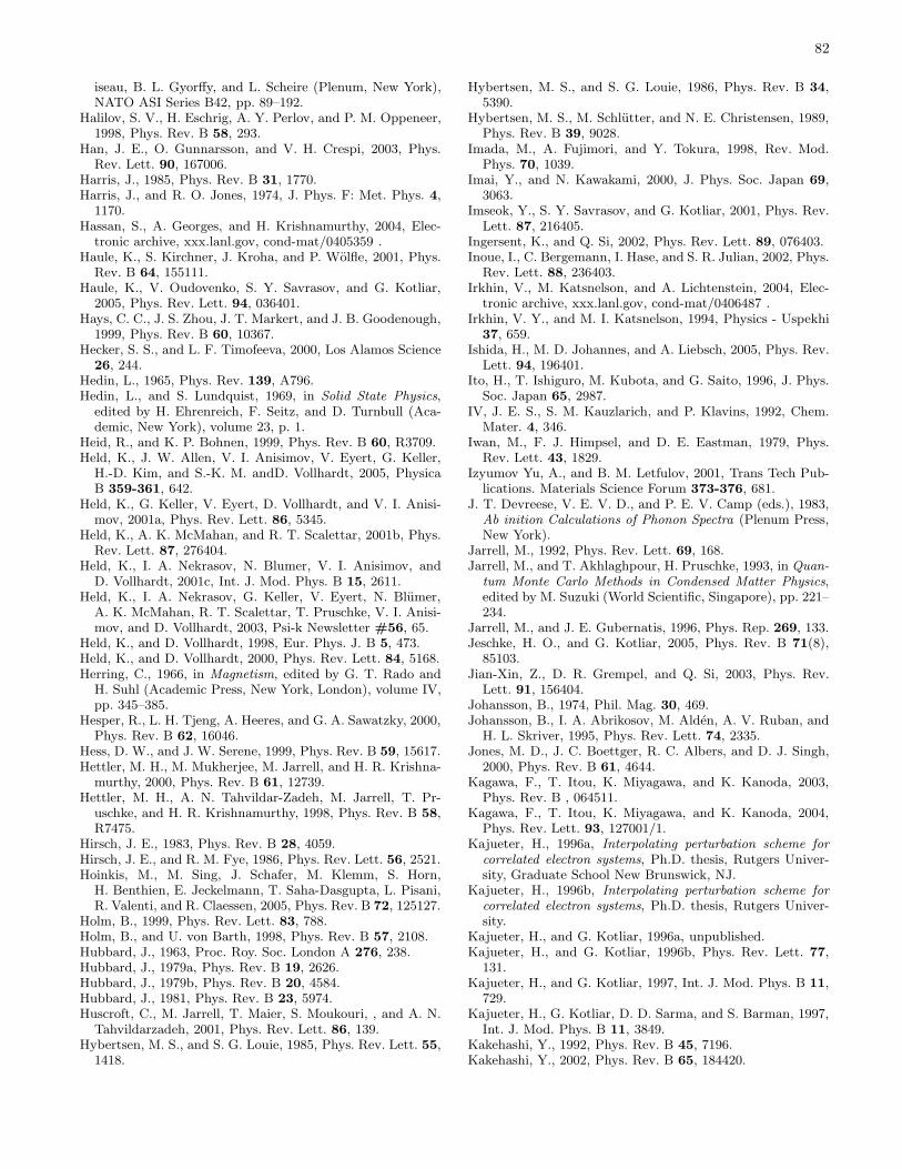
82

iseau, B. L. Gyorffy, and L. Scheire (Plenum, New York),NATO ASI Series B42, pp. 89–192.

Halilov, S. V., H. Eschrig, A. Y. Perlov, and P. M. Oppeneer,1998, Phys. Rev. B 58, 293.

Han, J. E., O. Gunnarsson, and V. H. Crespi, 2003, Phys.Rev. Lett. 90, 167006.

Harris, J., 1985, Phys. Rev. B 31, 1770.Harris, J., and R. O. Jones, 1974, J. Phys. F: Met. Phys. 4,

1170.Hassan, S., A. Georges, and H. Krishnamurthy, 2004, Elec-

tronic archive, xxx.lanl.gov, cond-mat/0405359 .Haule, K., S. Kirchner, J. Kroha, and P. Wolfle, 2001, Phys.

Rev. B 64, 155111.Haule, K., V. Oudovenko, S. Y. Savrasov, and G. Kotliar,

2005, Phys. Rev. Lett. 94, 036401.Hays, C. C., J. S. Zhou, J. T. Markert, and J. B. Goodenough,

1999, Phys. Rev. B 60, 10367.Hecker, S. S., and L. F. Timofeeva, 2000, Los Alamos Science

26, 244.Hedin, L., 1965, Phys. Rev. 139, A796.Hedin, L., and S. Lundquist, 1969, in Solid State Physics,

edited by H. Ehrenreich, F. Seitz, and D. Turnbull (Aca-demic, New York), volume 23, p. 1.

Heid, R., and K. P. Bohnen, 1999, Phys. Rev. B 60, R3709.Held, K., J. W. Allen, V. I. Anisimov, V. Eyert, G. Keller,

H.-D. Kim, and S.-K. M. andD. Vollhardt, 2005, PhysicaB 359-361, 642.

Held, K., G. Keller, V. Eyert, D. Vollhardt, and V. I. Anisi-mov, 2001a, Phys. Rev. Lett. 86, 5345.

Held, K., A. K. McMahan, and R. T. Scalettar, 2001b, Phys.Rev. Lett. 87, 276404.

Held, K., I. A. Nekrasov, N. Blumer, V. I. Anisimov, andD. Vollhardt, 2001c, Int. J. Mod. Phys. B 15, 2611.

Held, K., I. A. Nekrasov, G. Keller, V. Eyert, N. Blumer,A. K. McMahan, R. T. Scalettar, T. Pruschke, V. I. Anisi-mov, and D. Vollhardt, 2003, Psi-k Newsletter #56, 65.

Held, K., and D. Vollhardt, 1998, Eur. Phys. J. B 5, 473.Held, K., and D. Vollhardt, 2000, Phys. Rev. Lett. 84, 5168.Herring, C., 1966, in Magnetism, edited by G. T. Rado and

H. Suhl (Academic Press, New York, London), volume IV,pp. 345–385.

Hesper, R., L. H. Tjeng, A. Heeres, and G. A. Sawatzky, 2000,Phys. Rev. B 62, 16046.

Hess, D. W., and J. W. Serene, 1999, Phys. Rev. B 59, 15617.Hettler, M. H., M. Mukherjee, M. Jarrell, and H. R. Krishna-

murthy, 2000, Phys. Rev. B 61, 12739.Hettler, M. H., A. N. Tahvildar-Zadeh, M. Jarrell, T. Pr-

uschke, and H. R. Krishnamurthy, 1998, Phys. Rev. B 58,R7475.

Hirsch, J. E., 1983, Phys. Rev. B 28, 4059.Hirsch, J. E., and R. M. Fye, 1986, Phys. Rev. Lett. 56, 2521.Hoinkis, M., M. Sing, J. Schafer, M. Klemm, S. Horn,

H. Benthien, E. Jeckelmann, T. Saha-Dasgupta, L. Pisani,R. Valenti, and R. Claessen, 2005, Phys. Rev. B 72, 125127.

Holm, B., 1999, Phys. Rev. Lett. 83, 788.Holm, B., and U. von Barth, 1998, Phys. Rev. B 57, 2108.Hubbard, J., 1963, Proc. Roy. Soc. London A 276, 238.Hubbard, J., 1979a, Phys. Rev. B 19, 2626.Hubbard, J., 1979b, Phys. Rev. B 20, 4584.Hubbard, J., 1981, Phys. Rev. B 23, 5974.Huscroft, C., M. Jarrell, T. Maier, S. Moukouri, , and A. N.

Tahvildarzadeh, 2001, Phys. Rev. Lett. 86, 139.Hybertsen, M. S., and S. G. Louie, 1985, Phys. Rev. Lett. 55,

1418.

Hybertsen, M. S., and S. G. Louie, 1986, Phys. Rev. B 34,5390.

Hybertsen, M. S., M. Schlutter, and N. E. Christensen, 1989,Phys. Rev. B 39, 9028.

Imada, M., A. Fujimori, and Y. Tokura, 1998, Rev. Mod.Phys. 70, 1039.

Imai, Y., and N. Kawakami, 2000, J. Phys. Soc. Japan 69,3063.

Imseok, Y., S. Y. Savrasov, and G. Kotliar, 2001, Phys. Rev.Lett. 87, 216405.

Ingersent, K., and Q. Si, 2002, Phys. Rev. Lett. 89, 076403.Inoue, I., C. Bergemann, I. Hase, and S. R. Julian, 2002, Phys.

Rev. Lett. 88, 236403.Irkhin, V., M. Katsnelson, and A. Lichtenstein, 2004, Elec-

tronic archive, xxx.lanl.gov, cond-mat/0406487 .Irkhin, V. Y., and M. I. Katsnelson, 1994, Physics - Uspekhi

37, 659.Ishida, H., M. D. Johannes, and A. Liebsch, 2005, Phys. Rev.

Lett. 94, 196401.Ito, H., T. Ishiguro, M. Kubota, and G. Saito, 1996, J. Phys.

Soc. Japan 65, 2987.IV, J. E. S., S. M. Kauzlarich, and P. Klavins, 1992, Chem.

Mater. 4, 346.Iwan, M., F. J. Himpsel, and D. E. Eastman, 1979, Phys.

Rev. Lett. 43, 1829.Izyumov Yu, A., and B. M. Letfulov, 2001, Trans Tech Pub-

lications. Materials Science Forum 373-376, 681.J. T. Devreese, V. E. V. D., and P. E. V. Camp (eds.), 1983,

Ab inition Calculations of Phonon Spectra (Plenum Press,New York).

Jarrell, M., 1992, Phys. Rev. Lett. 69, 168.Jarrell, M., and T. Akhlaghpour, H. Pruschke, 1993, in Quan-

tum Monte Carlo Methods in Condensed Matter Physics,edited by M. Suzuki (World Scientific, Singapore), pp. 221–234.

Jarrell, M., and J. E. Gubernatis, 1996, Phys. Rep. 269, 133.Jeschke, H. O., and G. Kotliar, 2005, Phys. Rev. B 71(8),

85103.Jian-Xin, Z., D. R. Grempel, and Q. Si, 2003, Phys. Rev.

Lett. 91, 156404.Johansson, B., 1974, Phil. Mag. 30, 469.Johansson, B., I. A. Abrikosov, M. Alden, A. V. Ruban, and

H. L. Skriver, 1995, Phys. Rev. Lett. 74, 2335.Jones, M. D., J. C. Boettger, R. C. Albers, and D. J. Singh,

2000, Phys. Rev. B 61, 4644.Kagawa, F., T. Itou, K. Miyagawa, and K. Kanoda, 2003,

Phys. Rev. B , 064511.Kagawa, F., T. Itou, K. Miyagawa, and K. Kanoda, 2004,

Phys. Rev. Lett. 93, 127001/1.Kajueter, H., 1996a, Interpolating perturbation scheme for

correlated electron systems, Ph.D. thesis, Rutgers Univer-sity, Graduate School New Brunswick, NJ.

Kajueter, H., 1996b, Interpolating perturbation scheme for

correlated electron systems, Ph.D. thesis, Rutgers Univer-sity.

Kajueter, H., and G. Kotliar, 1996a, unpublished.Kajueter, H., and G. Kotliar, 1996b, Phys. Rev. Lett. 77,

131.Kajueter, H., and G. Kotliar, 1997, Int. J. Mod. Phys. B 11,

729.Kajueter, H., G. Kotliar, D. D. Sarma, and S. Barman, 1997,

Int. J. Mod. Phys. B 11, 3849.Kakehashi, Y., 1992, Phys. Rev. B 45, 7196.Kakehashi, Y., 2002, Phys. Rev. B 65, 184420.

83

Kakehashi, Y., S. Akbar, and N. Kimura, 1998, Phys. Rev. B57, 8354.

Kakizaki, A., J. Fujii, K. Shimada, A. Kamata, K. Ono,K. Park, T. Kinoshita, T. Ishii, and H. Fukutani, 1994,Phys. Rev. Lett. 72, 2781.

Kanamori, J., 1963, Prog. Theor. Phys. 30, 275.Kanoda, K., 2004, private communication.Katsnelson, M. I., and A. I. Lichtenstein, 2000, Phys. Rev. B

61, 8906.Katsnelson, M. I., and A. I. Lichtenstein, 2002, Eur. Phys. J.

B 30, 9.Keller, G., K. H. andV. Eyert, D. Vollhardt, and V. I. Anisi-

mov, 2005, Phys. Rev. B 70, 205116.Kikugawa, N., A. Mackenzie, C. Bergemann, and Y. Maeno,

2004, Phys. Rev. B 70, 174501.Kino, H., and H. Fukuyama, 1996, J. Phys. Soc. Japan 65,

2158.Kisker, E., K. Schroder, M. Campagna, and W. Gudat, 1984,

Phys. Rev. Lett. 52, 2285.Kobayashi, Y., S. Taniguchi, M. Kasai, M. Sato, T. Nishioka,

and M. Kontani, 1996, J. Phys. Soc. Japan 65, 3978.Koelling, D., and B. Harmon, 1977, JPC 10, 3107.Koga, A., N. Kawakami, T. Rice, and M. Sigrist, 2005, Elec-

tronic archive, xxx.lanl.gov, cond-mat/0503651 .Koga, A., N. Kawakami, T. M. Rice, and M. Sigrist, 2004,

Phys. Rev. Lett. 92, 216402.Korenman, V., J. L. Murray, and R. E. Prange, 1977a, Phys.

Rev. B 16, 4032.Korenman, V., J. L. Murray, and R. E. Prange, 1977b, Phys.

Rev. B 16, 4048.Korenman, V., J. L. Murray, and R. E. Prange, 1977c, Phys.

Rev. B 16, 4058.Kotani, T., 2000, J. Phys.: Condens. Matter 12, 2413.Kotliar, G., 1999a, Eur. Phys. J. B 11, 27.Kotliar, G., 1999b, Physica B 261, 711.Kotliar, G., 2001, in Open Problems in Strongly Corre-

lated Electron Systems, edited by J. Bonca, S. Sarkar,P. Prelovsek, and A. Ramsak (Kluwer Academic Publish-ers, Netherlands), NATO Science Series II, pp. 325–336.

Kotliar, G., 2003, Science 302, 67.Kotliar, G., 2005, J. Phys. Soc. Japan 74, 147.Kotliar, G., and H. Kajueter, 1996, Phys. Rev. B 54, R14221.Kotliar, G., E. Lange, and M. J. Rozenberg, 2000, Phys. Rev.

Lett. 84, 5180.Kotliar, G., S. Murthy, and M. J. Rozenberg, 2002, Phys.

Rev. Lett. 89, 046401.Kotliar, G., and A. E. Ruckenstein, 1986, Phys. Rev. Lett.

57, 1362.Kotliar, G., and S. Savrasov, 2001, in New Theoretical ap-

proaches to strongly correlated systems, edited by A. M.Tsvelik (Kluwer Academic Publishers, The Netherlands),pp. 259–301.

Kotliar, G., S. Y. Savrasov, G. Palsson, and G. Biroli, 2001,Phys. Rev. Lett. 87, 186401.

Kotliar, G., and D. Vollhardt, 2004, Physics Today 57, 53.Kreutz, T. J., T. Greber, P. Aebi, and J. Osterwalder, 1989,

Phys. Rev. B 58, 1300.Kroha, J., P. Wolfle, and T. A. Costi, 1997, Phys. Rev. Lett.

79, 261.Kubler, J., 2000, Theory of Itinerant Electron Magnetism

(Oxford University Press).Kuebler, J., 2002, Adv. Solid State Phys. 42, 407.Kumagai, K., T. Suzuki, Y. Taguchi, Y. Okada, Y. Fujishima,

and Y. Tokura, 1993, Phys. Rev. B 48, 7636.

Kutepov, A., and S. Kutepova, 2003, JPCM 15, 2607.Kuwamoto, H., J. M. Honig, and J. Appel, 1980, Phys. Rev.

B 22, 2626.Laad, M., L. Craco, and E. Muller-Hartmann, 2001, Phys.

Rev. B 64, 214421.Laad, M., L. Craco, and E. Muller-Hartmann, 2003a, Phys.

Rev. B 67, 033105.Laad, M., L. Craco, and E. Muller-Hartmann, 2003b, Phys.

Rev. Lett. 91, 156402.Lambin, P., and J. P. Vigneron, 1984, Phys. Rev. B 29, 3430.Lange, E., and G. Kotliar, 1999, Phys. Rev. B 59, 1800.Langreth, D. C., and J. P. Perdew, 1977, Phys. Rev. B 15,

2884.Lashley, J. C., A. C. Lawson, R. J. McQueeney, and

G. H. Lander, 2004, Electronic archive, xxx.lanl.gov, cond-mat/0410634 .

Lavagna, M., 1990, Phys. Rev. B 41, 142.Lechermann, F., S. Biermann, and A. Georges, 2005a, Phys.

Rev. Lett. 94, 166402.Lechermann, F., S. Biermann, and A. Georges, 2005b, Elec-

tronic archive, xxx.lanl.gov, cond-mat/0505241 .Lefebvre, S., P. Wzietek, S. Brown, C. Bourbonnais,

D. Jerome, C. Meziere, M. Fourmigue, and P. Batail, 2000,Phys. Rev. Lett. 85, 5420.

Li, T., P. Wolfle, and P. J. Hirschfeld, 1989, Phys. Rev. B 40,6817.

Lichtenstein, A., and A. Liebsch, 2002, in Ruthenate and

Rutheno-Cuprate Materials: Unconventional Superconduc-

tivity, Magnetism and Quantum Phase Transitions, editedby C. Noce, A. Vecchione, M. Cuoco, and A. Romano(Springer-Verlag, Berlin, Germany), pp. 76–90.

Lichtenstein, A. I., and M. I. Katsnelson, 1997, Bull. Am.Phys. 42, 573.

Lichtenstein, A. I., and M. I. Katsnelson, 1998, Phys. Rev. B57, 6884.

Lichtenstein, A. I., and M. I. Katsnelson, 2000, Phys. Rev. B62, R9283.

Lichtenstein, A. I., M. I. Katsnelson, and G. Kotliar, 2001,Phys. Rev. Lett. 87, 067205.

Lichtenstein, A. I., M. I. Katsnelson, and G. Kotliar, 2002a,in Electron Correlations and Materials Properties 2, editedby A. Gonis, N. Kioussis, and M. Ciftan (Kluwer Academic,Plenum Publishers, New York), p. 428.

Lichtenstein, A. I., M. I. Katsnelson, and G. Kotliar, 2002b,Electronic archive, xxx.lanl.gov, cond-mat/0211076 .

Liebsch, A., 1981, Phys. Rev. B 23, 5203.Liebsch, A., 2003a, Europhys. Lett. 63, 97.Liebsch, A., 2003b, Phys. Rev. Lett. 91, 226401.Liebsch, A., 2003c, Phys. Rev. Lett. 90, 096401.Liebsch, A., and A. Lichtenstein, 2000a, Phys. Rev. Lett. 84,

1591.Liebsch, A., and A. Lichtenstein, 2000b, Phys. Rev. Lett. 84,

1591.Liechtenstein, A. I., M. I. Katsnelson, V. P. Antropov, and

V. A. Gubanov, 1987, J. Magn. Magn. Mater. 67, 65.Lima, N. A., L. N. Oliveira, and K. Capelle, 2002, Europhys.

Lett. 60, 601.Limelette, P., A. Georges, D. Jerome, P. Wzietek, P. Metcalf,

and J. M. Honig, 2003a, Science 302, 89.Limelette, P., P. Wzietek, S. Florens, A. Georges, T. A. Costi,

C. Pasquier, D. Jerome, C. Meziere, and P. Batail, 2003b,Phys. Rev. Lett. 91, 016401.

Lindbaum, A., S. Heathman, K. Litfin, Y. Meresse, R. G.Haire, T. L. Bihan, and H. Libotte, 2001, Phys. Rev. B 63,

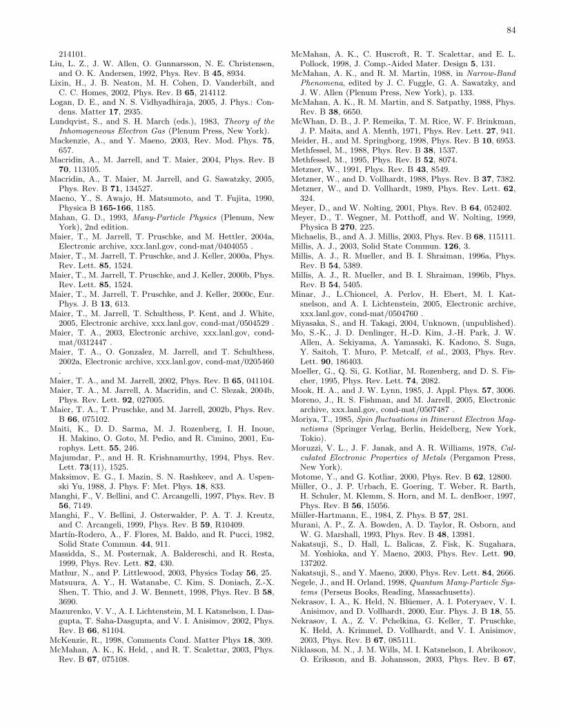
84

214101.Liu, L. Z., J. W. Allen, O. Gunnarsson, N. E. Christensen,

and O. K. Andersen, 1992, Phys. Rev. B 45, 8934.Lixin, H., J. B. Neaton, M. H. Cohen, D. Vanderbilt, and

C. C. Homes, 2002, Phys. Rev. B 65, 214112.Logan, D. E., and N. S. Vidhyadhiraja, 2005, J. Phys.: Con-

dens. Matter 17, 2935.Lundqvist, S., and S. H. March (eds.), 1983, Theory of the

Inhomogeneous Electron Gas (Plenum Press, New York).Mackenzie, A., and Y. Maeno, 2003, Rev. Mod. Phys. 75,

657.Macridin, A., M. Jarrell, and T. Maier, 2004, Phys. Rev. B

70, 113105.Macridin, A., T. Maier, M. Jarrell, and G. Sawatzky, 2005,

Phys. Rev. B 71, 134527.Maeno, Y., S. Awajo, H. Matsumoto, and T. Fujita, 1990,

Physica B 165-166, 1185.Mahan, G. D., 1993, Many-Particle Physics (Plenum, New

York), 2nd edition.Maier, T., M. Jarrell, T. Pruschke, and M. Hettler, 2004a,

Electronic archive, xxx.lanl.gov, cond-mat/0404055 .Maier, T., M. Jarrell, T. Pruschke, and J. Keller, 2000a, Phys.

Rev. Lett. 85, 1524.Maier, T., M. Jarrell, T. Pruschke, and J. Keller, 2000b, Phys.

Rev. Lett. 85, 1524.Maier, T., M. Jarrell, T. Pruschke, and J. Keller, 2000c, Eur.

Phys. J. B 13, 613.Maier, T., M. Jarrell, T. Schulthess, P. Kent, and J. White,

2005, Electronic archive, xxx.lanl.gov, cond-mat/0504529 .Maier, T. A., 2003, Electronic archive, xxx.lanl.gov, cond-

mat/0312447 .Maier, T. A., O. Gonzalez, M. Jarrell, and T. Schulthess,

2002a, Electronic archive, xxx.lanl.gov, cond-mat/0205460.

Maier, T. A., and M. Jarrell, 2002, Phys. Rev. B 65, 041104.Maier, T. A., M. Jarrell, A. Macridin, and C. Slezak, 2004b,

Phys. Rev. Lett. 92, 027005.Maier, T. A., T. Pruschke, and M. Jarrell, 2002b, Phys. Rev.

B 66, 075102.Maiti, K., D. D. Sarma, M. J. Rozenberg, I. H. Inoue,

H. Makino, O. Goto, M. Pedio, and R. Cimino, 2001, Eu-rophys. Lett. 55, 246.

Majumdar, P., and H. R. Krishnamurthy, 1994, Phys. Rev.Lett. 73(11), 1525.

Maksimov, E. G., I. Mazin, S. N. Rashkeev, and A. Uspen-ski Yu, 1988, J. Phys. F: Met. Phys. 18, 833.

Manghi, F., V. Bellini, and C. Arcangelli, 1997, Phys. Rev. B56, 7149.

Manghi, F., V. Bellini, J. Osterwalder, P. A. T. J. Kreutz,and C. Arcangeli, 1999, Phys. Rev. B 59, R10409.

Martın-Rodero, A., F. Flores, M. Baldo, and R. Pucci, 1982,Solid State Commun. 44, 911.

Massidda, S., M. Posternak, A. Baldereschi, and R. Resta,1999, Phys. Rev. Lett. 82, 430.

Mathur, N., and P. Littlewood, 2003, Physics Today 56, 25.Matsuura, A. Y., H. Watanabe, C. Kim, S. Doniach, Z.-X.

Shen, T. Thio, and J. W. Bennett, 1998, Phys. Rev. B 58,3690.

Mazurenko, V. V., A. I. Lichtenstein, M. I. Katsnelson, I. Das-gupta, T. Saha-Dasgupta, and V. I. Anisimov, 2002, Phys.Rev. B 66, 81104.

McKenzie, R., 1998, Comments Cond. Matter Phys 18, 309.McMahan, A. K., K. Held, , and R. T. Scalettar, 2003, Phys.

Rev. B 67, 075108.

McMahan, A. K., C. Huscroft, R. T. Scalettar, and E. L.Pollock, 1998, J. Comp.-Aided Mater. Design 5, 131.

McMahan, A. K., and R. M. Martin, 1988, in Narrow-Band

Phenomena, edited by J. C. Fuggle, G. A. Sawatzky, andJ. W. Allen (Plenum Press, New York), p. 133.

McMahan, A. K., R. M. Martin, and S. Satpathy, 1988, Phys.Rev. B 38, 6650.

McWhan, D. B., J. P. Remeika, T. M. Rice, W. F. Brinkman,J. P. Maita, and A. Menth, 1971, Phys. Rev. Lett. 27, 941.

Meider, H., and M. Springborg, 1998, Phys. Rev. B 10, 6953.Methfessel, M., 1988, Phys. Rev. B 38, 1537.Methfessel, M., 1995, Phys. Rev. B 52, 8074.Metzner, W., 1991, Phys. Rev. B 43, 8549.Metzner, W., and D. Vollhardt, 1988, Phys. Rev. B 37, 7382.Metzner, W., and D. Vollhardt, 1989, Phys. Rev. Lett. 62,

324.Meyer, D., and W. Nolting, 2001, Phys. Rev. B 64, 052402.Meyer, D., T. Wegner, M. Potthoff, and W. Nolting, 1999,

Physica B 270, 225.Michaelis, B., and A. J. Millis, 2003, Phys. Rev. B 68, 115111.Millis, A. J., 2003, Solid State Commun. 126, 3.Millis, A. J., R. Mueller, and B. I. Shraiman, 1996a, Phys.

Rev. B 54, 5389.Millis, A. J., R. Mueller, and B. I. Shraiman, 1996b, Phys.

Rev. B 54, 5405.Minar, J., L.Chioncel, A. Perlov, H. Ebert, M. I. Kat-

snelson, and A. I. Lichtenstein, 2005, Electronic archive,xxx.lanl.gov, cond-mat/0504760 .

Miyasaka, S., and H. Takagi, 2004, Unknown, (unpublished).Mo, S.-K., J. D. Denlinger, H.-D. Kim, J.-H. Park, J. W.

Allen, A. Sekiyama, A. Yamasaki, K. Kadono, S. Suga,Y. Saitoh, T. Muro, P. Metcalf, et al., 2003, Phys. Rev.Lett. 90, 186403.

Moeller, G., Q. Si, G. Kotliar, M. Rozenberg, and D. S. Fis-cher, 1995, Phys. Rev. Lett. 74, 2082.

Mook, H. A., and J. W. Lynn, 1985, J. Appl. Phys. 57, 3006.Moreno, J., R. S. Fishman, and M. Jarrell, 2005, Electronic

archive, xxx.lanl.gov, cond-mat/0507487 .Moriya, T., 1985, Spin fluctuations in Itinerant Electron Mag-

netisms (Springer Verlag, Berlin, Heidelberg, New York,Tokio).

Moruzzi, V. L., J. F. Janak, and A. R. Williams, 1978, Cal-

culated Electronic Properties of Metals (Pergamon Press,New York).

Motome, Y., and G. Kotliar, 2000, Phys. Rev. B 62, 12800.Muller, O., J. P. Urbach, E. Goering, T. Weber, R. Barth,

H. Schuler, M. Klemm, S. Horn, and M. L. denBoer, 1997,Phys. Rev. B 56, 15056.

Muller-Hartmann, E., 1984, Z. Phys. B 57, 281.Murani, A. P., Z. A. Bowden, A. D. Taylor, R. Osborn, and

W. G. Marshall, 1993, Phys. Rev. B 48, 13981.Nakatsuji, S., D. Hall, L. Balicas, Z. Fisk, K. Sugahara,

M. Yoshioka, and Y. Maeno, 2003, Phys. Rev. Lett. 90,137202.

Nakatsuji, S., and Y. Maeno, 2000, Phys. Rev. Lett. 84, 2666.Negele, J., and H. Orland, 1998, Quantum Many-Particle Sys-

tems (Perseus Books, Reading, Massachusetts).Nekrasov, I. A., K. Held, N. Bluemer, A. I. Poteryaev, V. I.

Anisimov, and D. Vollhardt, 2000, Eur. Phys. J. B 18, 55.Nekrasov, I. A., Z. V. Pchelkina, G. Keller, T. Pruschke,

K. Held, A. Krimmel, D. Vollhardt, and V. I. Anisimov,2003, Phys. Rev. B 67, 085111.

Niklasson, M. N., J. M. Wills, M. I. Katsnelson, I. Abrikosov,O. Eriksson, and B. Johansson, 2003, Phys. Rev. B 67,

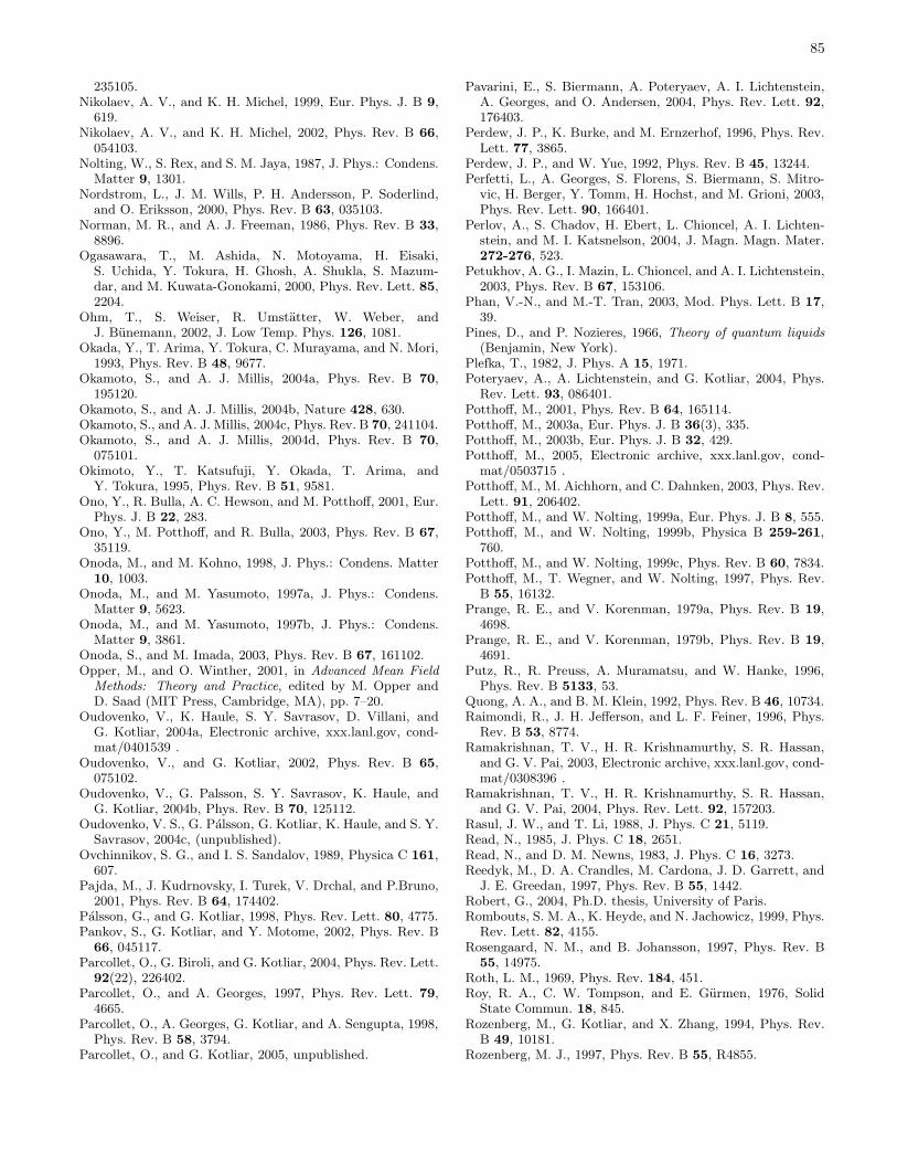
85

235105.Nikolaev, A. V., and K. H. Michel, 1999, Eur. Phys. J. B 9,

619.Nikolaev, A. V., and K. H. Michel, 2002, Phys. Rev. B 66,

054103.Nolting, W., S. Rex, and S. M. Jaya, 1987, J. Phys.: Condens.

Matter 9, 1301.Nordstrom, L., J. M. Wills, P. H. Andersson, P. Soderlind,

and O. Eriksson, 2000, Phys. Rev. B 63, 035103.Norman, M. R., and A. J. Freeman, 1986, Phys. Rev. B 33,

8896.Ogasawara, T., M. Ashida, N. Motoyama, H. Eisaki,

S. Uchida, Y. Tokura, H. Ghosh, A. Shukla, S. Mazum-dar, and M. Kuwata-Gonokami, 2000, Phys. Rev. Lett. 85,2204.

Ohm, T., S. Weiser, R. Umstatter, W. Weber, andJ. Bunemann, 2002, J. Low Temp. Phys. 126, 1081.

Okada, Y., T. Arima, Y. Tokura, C. Murayama, and N. Mori,1993, Phys. Rev. B 48, 9677.

Okamoto, S., and A. J. Millis, 2004a, Phys. Rev. B 70,195120.

Okamoto, S., and A. J. Millis, 2004b, Nature 428, 630.Okamoto, S., and A. J. Millis, 2004c, Phys. Rev. B 70, 241104.Okamoto, S., and A. J. Millis, 2004d, Phys. Rev. B 70,

075101.Okimoto, Y., T. Katsufuji, Y. Okada, T. Arima, and

Y. Tokura, 1995, Phys. Rev. B 51, 9581.Ono, Y., R. Bulla, A. C. Hewson, and M. Potthoff, 2001, Eur.

Phys. J. B 22, 283.Ono, Y., M. Potthoff, and R. Bulla, 2003, Phys. Rev. B 67,

35119.Onoda, M., and M. Kohno, 1998, J. Phys.: Condens. Matter

10, 1003.Onoda, M., and M. Yasumoto, 1997a, J. Phys.: Condens.

Matter 9, 5623.Onoda, M., and M. Yasumoto, 1997b, J. Phys.: Condens.

Matter 9, 3861.Onoda, S., and M. Imada, 2003, Phys. Rev. B 67, 161102.Opper, M., and O. Winther, 2001, in Advanced Mean Field

Methods: Theory and Practice, edited by M. Opper andD. Saad (MIT Press, Cambridge, MA), pp. 7–20.

Oudovenko, V., K. Haule, S. Y. Savrasov, D. Villani, andG. Kotliar, 2004a, Electronic archive, xxx.lanl.gov, cond-mat/0401539 .

Oudovenko, V., and G. Kotliar, 2002, Phys. Rev. B 65,075102.

Oudovenko, V., G. Palsson, S. Y. Savrasov, K. Haule, andG. Kotliar, 2004b, Phys. Rev. B 70, 125112.

Oudovenko, V. S., G. Palsson, G. Kotliar, K. Haule, and S. Y.Savrasov, 2004c, (unpublished).

Ovchinnikov, S. G., and I. S. Sandalov, 1989, Physica C 161,607.

Pajda, M., J. Kudrnovsky, I. Turek, V. Drchal, and P.Bruno,2001, Phys. Rev. B 64, 174402.

Palsson, G., and G. Kotliar, 1998, Phys. Rev. Lett. 80, 4775.Pankov, S., G. Kotliar, and Y. Motome, 2002, Phys. Rev. B

66, 045117.Parcollet, O., G. Biroli, and G. Kotliar, 2004, Phys. Rev. Lett.

92(22), 226402.Parcollet, O., and A. Georges, 1997, Phys. Rev. Lett. 79,

4665.Parcollet, O., A. Georges, G. Kotliar, and A. Sengupta, 1998,

Phys. Rev. B 58, 3794.Parcollet, O., and G. Kotliar, 2005, unpublished.

Pavarini, E., S. Biermann, A. Poteryaev, A. I. Lichtenstein,A. Georges, and O. Andersen, 2004, Phys. Rev. Lett. 92,176403.

Perdew, J. P., K. Burke, and M. Ernzerhof, 1996, Phys. Rev.Lett. 77, 3865.

Perdew, J. P., and W. Yue, 1992, Phys. Rev. B 45, 13244.Perfetti, L., A. Georges, S. Florens, S. Biermann, S. Mitro-

vic, H. Berger, Y. Tomm, H. Hochst, and M. Grioni, 2003,Phys. Rev. Lett. 90, 166401.

Perlov, A., S. Chadov, H. Ebert, L. Chioncel, A. I. Lichten-stein, and M. I. Katsnelson, 2004, J. Magn. Magn. Mater.272-276, 523.

Petukhov, A. G., I. Mazin, L. Chioncel, and A. I. Lichtenstein,2003, Phys. Rev. B 67, 153106.

Phan, V.-N., and M.-T. Tran, 2003, Mod. Phys. Lett. B 17,39.

Pines, D., and P. Nozieres, 1966, Theory of quantum liquids

(Benjamin, New York).Plefka, T., 1982, J. Phys. A 15, 1971.Poteryaev, A., A. Lichtenstein, and G. Kotliar, 2004, Phys.

Rev. Lett. 93, 086401.Potthoff, M., 2001, Phys. Rev. B 64, 165114.Potthoff, M., 2003a, Eur. Phys. J. B 36(3), 335.Potthoff, M., 2003b, Eur. Phys. J. B 32, 429.Potthoff, M., 2005, Electronic archive, xxx.lanl.gov, cond-

mat/0503715 .Potthoff, M., M. Aichhorn, and C. Dahnken, 2003, Phys. Rev.

Lett. 91, 206402.Potthoff, M., and W. Nolting, 1999a, Eur. Phys. J. B 8, 555.Potthoff, M., and W. Nolting, 1999b, Physica B 259-261,

760.Potthoff, M., and W. Nolting, 1999c, Phys. Rev. B 60, 7834.Potthoff, M., T. Wegner, and W. Nolting, 1997, Phys. Rev.

B 55, 16132.Prange, R. E., and V. Korenman, 1979a, Phys. Rev. B 19,

4698.Prange, R. E., and V. Korenman, 1979b, Phys. Rev. B 19,

4691.Putz, R., R. Preuss, A. Muramatsu, and W. Hanke, 1996,

Phys. Rev. B 5133, 53.Quong, A. A., and B. M. Klein, 1992, Phys. Rev. B 46, 10734.Raimondi, R., J. H. Jefferson, and L. F. Feiner, 1996, Phys.

Rev. B 53, 8774.Ramakrishnan, T. V., H. R. Krishnamurthy, S. R. Hassan,

and G. V. Pai, 2003, Electronic archive, xxx.lanl.gov, cond-mat/0308396 .

Ramakrishnan, T. V., H. R. Krishnamurthy, S. R. Hassan,and G. V. Pai, 2004, Phys. Rev. Lett. 92, 157203.

Rasul, J. W., and T. Li, 1988, J. Phys. C 21, 5119.Read, N., 1985, J. Phys. C 18, 2651.Read, N., and D. M. Newns, 1983, J. Phys. C 16, 3273.Reedyk, M., D. A. Crandles, M. Cardona, J. D. Garrett, and

J. E. Greedan, 1997, Phys. Rev. B 55, 1442.Robert, G., 2004, Ph.D. thesis, University of Paris.Rombouts, S. M. A., K. Heyde, and N. Jachowicz, 1999, Phys.

Rev. Lett. 82, 4155.Rosengaard, N. M., and B. Johansson, 1997, Phys. Rev. B

55, 14975.Roth, L. M., 1969, Phys. Rev. 184, 451.Roy, R. A., C. W. Tompson, and E. Gurmen, 1976, Solid

State Commun. 18, 845.Rozenberg, M., G. Kotliar, and X. Zhang, 1994, Phys. Rev.

B 49, 10181.Rozenberg, M. J., 1997, Phys. Rev. B 55, R4855.

86

Rozenberg, M. J., G. K. H. Kajueter, G. A. Thomas, D. H.Rapkine, J. M. Honig, and P. Metcalf, 1995, Phys. Rev.Lett. 75, 105.

Rozenberg, M. J., G. Kotliar, and H. Kajueter, 1996, Phys.Rev. B 54, 8452.

Rozenberg, M. J., X. Y. Zhang, and G. Kotliar, 1992, Phys.Rev. Lett. 69, 1236.

Rubtsov, A., 2003, Electronic archive, xxx.lanl.gov, cond-mat/0302228 .

Rubtsov, A. N., V. V. Savkin, and A. I. Lichtenstein, 2004,Electronic archive, xxx.lanl.gov, cond-mat/0411344 .

Sachdev, S., and J. Ye, 1993, Phys. Rev. Lett. 70, 3339.Saha-Dasgupta, T., A. Lichtenstein, and R. Valenti, 2005a,

Phys. Rev. B 71, 153108.Saha-Dasgupta, T., A. Lichtenstein, and R. Valenti, 2005b,

Phys. Rev. B 71, 153108.Sales, B. C., D. Mandrus, and R. K. Williams, 1996, Science

272, 1325.Sarma, D., S. Barman, H. Kajueter, and G. Kotliar, 1996,

Europhys. Lett. 36, 307.Savkin, V. V., A. N. Rubtsov, M. I. Katsnelson, and A. I.

Lichtenstein, 2005, Phys. Rev. Lett. 94, 026402.Savrasov, S. Y., 1992, Phys. Rev. Lett. 69, 2819.Savrasov, S. Y., 1996, Phys. Rev. B 54, 16470.Savrasov, S. Y., K. Haule, and G. Kotliar, 2005, Electronic

archive, xxx.lanl.gov, cond-mat/0507552 .Savrasov, S. Y., and G. Kotliar, 2000, Phys. Rev. Lett. 84,

3670.Savrasov, S. Y., and G. Kotliar, 2003, Phys. Rev. Lett. 90,

056401.Savrasov, S. Y., and G. Kotliar, 2004a, Phys. Rev. B 69,

245101.Savrasov, S. Y., and G. Kotliar, 2004b, Phys. Rev. B 69,

245101.Savrasov, S. Y., G. Kotliar, and E. Abrahams, 2001, Nature

410, 793.Savrasov, S. Y., V. Oudovenko, K. Haule, D. Villani, and

G. Kotliar, 2004, Electronic archive, xxx.lanl.gov, cond-mat/0410410 .

Sawatzky, G. A., 1995, in Spectroscopy of Mott Insulators

and Correlated Metals, edited by A. Fujimori and Y.Tokura(Springer-Verlag, Berlin), volume 119.

Schlesinger, Z., Z. Fisk, H. T. Zhang, M. B. Maple, J. F.DiTusa, and G. Aeppli, 1993, Phys. Rev. Lett. 71, 1748.

Schonhammer, K., O. Gunnarsson, and R. M. Noack, 1995,Phys. Rev. B 52, 2504.

Seidel, A., C. Marianetti, F. Chou, G. Ceder, and P. Lee,2003, Phys. Rev. B 67, 020405.

Sekiyama, A., H. Fujiwara, S. Imada, H. Eisaki, S. I. Uchida,K. Takegahara, H. Harima, Y. Saitoh, and S. Suga, 2002,Electronic archive, xxx.lanl.gov, cond-mat/0206471 .

Sekiyama, A., H. Fujiwara, S. Imada, S. Suga, H. Eisaki,S. I. Uchida, K. Takegahara, H. Harima, Y. Saitoh, I. A.Nekrasov, G. Keller, D. E. Kondakov, et al., 2004, Phys.Rev. Lett. 93, 156402.

Senechal, D., D. Perez, and M. Pioro-Ladriere, 2000, Phys.Rev. Lett. 84, 522.

Senechal, D., D. Perez, and D. Plouffe, 2002, Phys. Rev. B66, 075129.

Senechal, D., and A. M. Tremblay, 2004, Phys. Rev. Lett. 92,126401.

Sengupta, A. M., and A. Georges, 1995, Phys. Rev. B 52,10295.

Setty, A., and B. R. Cooper, 2003, Bulletin of March Meeting

of American Physical Society Abstract G15.007.Shankar, R., 1994, Rev. Mod. Phys. 66, 129.Shvaika, A. M., 2000, Phys. Rev. B 62, 2358.Si, Q., 2001, J. Magn. Magn. Mater. 226-230, 30.Si, Q., 2003, J. Phys.: Condens. Matter 15, S2207.Si, Q., S. Rabello, K. Ingersent, and J. L. Smith, 2003, Phys.

Rev. B 68, 115103.Si, Q., and J. L. Smith, 1996, Phys. Rev. Lett. 77, 3391.Si, Q. M., S. Rabello, K. Ingersent, and J. L. Smith, 2001,

Nature 413, 804.Sinkovic, B., L. H. Tjeng, N. B. Brookes, J. B. Goedkoop,

R. Hesper, E. Pellegrin, F. M. F. de Groot, S. Altieri, S. L.Hulbert, E. Shekel, and G. A. Sawatzky, 1997, Phys. Rev.B 79, 3510.

Smith, J. L., and Q. Si, 2000, Phys. Rev. B 61, 5184.Smith, V. E., D. E. Logan, and H. R. Krishnamurthy, 2003,

Eur. Phys. J. B 32, 49.Soderland, P., and B. Sadigh, 2004, Phys. Rev. Lett. 92,

185702.Soderlind, P., 2001, Europhys. Lett. 55, 525.Soderlind, P., O. Eriksson, B. Johansson, and J. M. Wills,

1994, Phys. Rev. B 50, 7291.Soderlind, P., A. Landa, and B. Sadigh, 2002, Phys. Rev. B

66, 205109.Solovyev, I. V., A. I. Liechtenstein, V. A. Gubanov, V. P.

Antropov, and O. K. Andersen, 1991, Phys. Rev. B 43,14414.

Springer, M., and F. Aryasetiawan, 1998, Phys. Rev. B 57,4364.

Sreedhar, K., M. McElfresh, D. Perry, D. Kim, P. Metcalf,and J. M. Honig, 1994, J. Solid State Chem. 110, 208.

Stanescu, T., 2005, unpublished.Staunton, J., B. L. Gyorffy, A. J. Pindor, G. M. Stocks, and

H. Winter, 1985, J. Phys. F: Met. Phys. 15, 1387.Steiner, M. M., R. C. Albers, and L. J. Sham, 1992, Phys.

Rev. B 45, 13272.Stewart, G. R., 2001, Rev. Mod. Phys. 73, 797.Stocks, G. M., B. Ujfalussy, X. Wang, Y. Wang, D. M. C.

Nicholson, W. A. Shelton, A. Canning, and B. L. Gyorffy,1998, Phil. Mag. 78, 665.

Stratonovich, R., 1958, Sov. Phys. Dokl. 2, 416.Sun, P., and G. Kotliar, 2002, Phys. Rev. B 66, 85120.Sun, P., and G. Kotliar, 2003, Phys. Rev. Lett. 91, 037209.Sun, P., and G. Kotliar, 2004, Phys. Rev. Lett. 92, 196402.Svane, A., and O. Gunnarsson, 1990, Phys. Rev. Lett. 65,

1148.Svane, A., W. Temmerman, and Z. Szotek, 1999, Phys. Rev.

B 59, 7888.Szotek, Z., W. M. Temmerman, and H. Winter, 1993, Phys.

Rev. B 47, 4029.Takegahara, K., 1993, J. Phys. Soc. Japan 62, 1736.Takenobu, T., T. Muro, Y. Iwasa, and T. Mitani, 2000, Phys.

Rev. Lett. 85, 381.Tiago, M. L., S. Ismail-Beigi, and S. G. Louie, 2003, Elec-

tronic archive, xxx.lanl.gov, cond-mat/0307181 .Tokura, Y. (ed.), 1990, Colossal Magnetoresistive Oxides

(Gordon and Breach, Amsterdam).Tokura, Y., 2003, Physics Today 56, 50.Tokura, Y., Y. Taguchi, Y. Okada, Y. Fujishima, T. Arima,

K. Kumagai, and Y. Iye, 1993, Phys. Rev. Lett. 70, 2126.Tong, N.-H., 2005, Electronic archive, xxx.lanl.gov, cond-

mat/0504778 .Toropova, A., G. Kotliar, S. Y. Savrasov, and V. S.

Oudovenko, 2005, Phys. Rev. B 71, 172403.

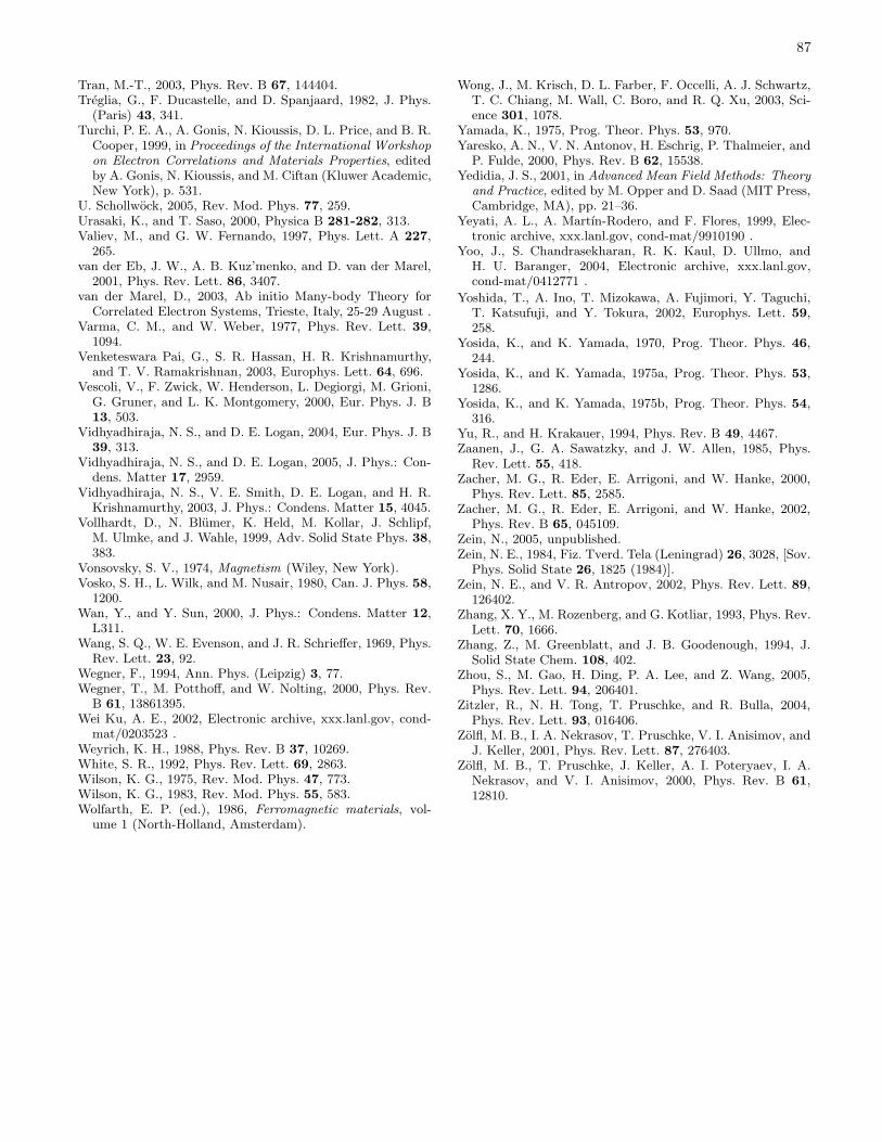
87

Tran, M.-T., 2003, Phys. Rev. B 67, 144404.Treglia, G., F. Ducastelle, and D. Spanjaard, 1982, J. Phys.

(Paris) 43, 341.Turchi, P. E. A., A. Gonis, N. Kioussis, D. L. Price, and B. R.

Cooper, 1999, in Proceedings of the International Workshop

on Electron Correlations and Materials Properties, editedby A. Gonis, N. Kioussis, and M. Ciftan (Kluwer Academic,New York), p. 531.

U. Schollwock, 2005, Rev. Mod. Phys. 77, 259.Urasaki, K., and T. Saso, 2000, Physica B 281-282, 313.Valiev, M., and G. W. Fernando, 1997, Phys. Lett. A 227,

265.van der Eb, J. W., A. B. Kuz’menko, and D. van der Marel,

2001, Phys. Rev. Lett. 86, 3407.van der Marel, D., 2003, Ab initio Many-body Theory for

Correlated Electron Systems, Trieste, Italy, 25-29 August .Varma, C. M., and W. Weber, 1977, Phys. Rev. Lett. 39,

1094.Venketeswara Pai, G., S. R. Hassan, H. R. Krishnamurthy,

and T. V. Ramakrishnan, 2003, Europhys. Lett. 64, 696.Vescoli, V., F. Zwick, W. Henderson, L. Degiorgi, M. Grioni,

G. Gruner, and L. K. Montgomery, 2000, Eur. Phys. J. B13, 503.

Vidhyadhiraja, N. S., and D. E. Logan, 2004, Eur. Phys. J. B39, 313.

Vidhyadhiraja, N. S., and D. E. Logan, 2005, J. Phys.: Con-dens. Matter 17, 2959.

Vidhyadhiraja, N. S., V. E. Smith, D. E. Logan, and H. R.Krishnamurthy, 2003, J. Phys.: Condens. Matter 15, 4045.

Vollhardt, D., N. Blumer, K. Held, M. Kollar, J. Schlipf,M. Ulmke, and J. Wahle, 1999, Adv. Solid State Phys. 38,383.

Vonsovsky, S. V., 1974, Magnetism (Wiley, New York).Vosko, S. H., L. Wilk, and M. Nusair, 1980, Can. J. Phys. 58,

1200.Wan, Y., and Y. Sun, 2000, J. Phys.: Condens. Matter 12,

L311.Wang, S. Q., W. E. Evenson, and J. R. Schrieffer, 1969, Phys.

Rev. Lett. 23, 92.Wegner, F., 1994, Ann. Phys. (Leipzig) 3, 77.Wegner, T., M. Potthoff, and W. Nolting, 2000, Phys. Rev.

B 61, 13861395.Wei Ku, A. E., 2002, Electronic archive, xxx.lanl.gov, cond-

mat/0203523 .Weyrich, K. H., 1988, Phys. Rev. B 37, 10269.White, S. R., 1992, Phys. Rev. Lett. 69, 2863.Wilson, K. G., 1975, Rev. Mod. Phys. 47, 773.Wilson, K. G., 1983, Rev. Mod. Phys. 55, 583.Wolfarth, E. P. (ed.), 1986, Ferromagnetic materials, vol-

ume 1 (North-Holland, Amsterdam).

Wong, J., M. Krisch, D. L. Farber, F. Occelli, A. J. Schwartz,T. C. Chiang, M. Wall, C. Boro, and R. Q. Xu, 2003, Sci-ence 301, 1078.

Yamada, K., 1975, Prog. Theor. Phys. 53, 970.Yaresko, A. N., V. N. Antonov, H. Eschrig, P. Thalmeier, and

P. Fulde, 2000, Phys. Rev. B 62, 15538.Yedidia, J. S., 2001, in Advanced Mean Field Methods: Theory

and Practice, edited by M. Opper and D. Saad (MIT Press,Cambridge, MA), pp. 21–36.

Yeyati, A. L., A. Martın-Rodero, and F. Flores, 1999, Elec-tronic archive, xxx.lanl.gov, cond-mat/9910190 .

Yoo, J., S. Chandrasekharan, R. K. Kaul, D. Ullmo, andH. U. Baranger, 2004, Electronic archive, xxx.lanl.gov,cond-mat/0412771 .

Yoshida, T., A. Ino, T. Mizokawa, A. Fujimori, Y. Taguchi,T. Katsufuji, and Y. Tokura, 2002, Europhys. Lett. 59,258.

Yosida, K., and K. Yamada, 1970, Prog. Theor. Phys. 46,244.

Yosida, K., and K. Yamada, 1975a, Prog. Theor. Phys. 53,1286.

Yosida, K., and K. Yamada, 1975b, Prog. Theor. Phys. 54,316.

Yu, R., and H. Krakauer, 1994, Phys. Rev. B 49, 4467.Zaanen, J., G. A. Sawatzky, and J. W. Allen, 1985, Phys.

Rev. Lett. 55, 418.Zacher, M. G., R. Eder, E. Arrigoni, and W. Hanke, 2000,

Phys. Rev. Lett. 85, 2585.Zacher, M. G., R. Eder, E. Arrigoni, and W. Hanke, 2002,

Phys. Rev. B 65, 045109.Zein, N., 2005, unpublished.Zein, N. E., 1984, Fiz. Tverd. Tela (Leningrad) 26, 3028, [Sov.

Phys. Solid State 26, 1825 (1984)].Zein, N. E., and V. R. Antropov, 2002, Phys. Rev. Lett. 89,

126402.Zhang, X. Y., M. Rozenberg, and G. Kotliar, 1993, Phys. Rev.

Lett. 70, 1666.Zhang, Z., M. Greenblatt, and J. B. Goodenough, 1994, J.

Solid State Chem. 108, 402.Zhou, S., M. Gao, H. Ding, P. A. Lee, and Z. Wang, 2005,

Phys. Rev. Lett. 94, 206401.Zitzler, R., N. H. Tong, T. Pruschke, and R. Bulla, 2004,

Phys. Rev. Lett. 93, 016406.Zolfl, M. B., I. A. Nekrasov, T. Pruschke, V. I. Anisimov, and

J. Keller, 2001, Phys. Rev. Lett. 87, 276403.Zolfl, M. B., T. Pruschke, J. Keller, A. I. Poteryaev, I. A.

Nekrasov, and V. I. Anisimov, 2000, Phys. Rev. B 61,12810.