Electronic Colloquium on ... - logique.jussieu.frnderugy/doc/VPCompletECCC.pdfElectronic Colloquium...

Homomorphism Polynomials complete for VP∗

Arnaud Durand1, Meena Mahajan2, Guillaume Malod1, Nicolas deRugy-Altherre 1, and Nitin Saurabh2

1 Univ Paris Diderot, Sorbonne Paris Cité, IMJ-PRG, UMR 7586 CNRS,Sorbonne Université, UPMC Univ Paris 06, F-75013, Paris, France.{durand,malod,nderugy}@math.univ-paris-diderot.fr

2 The Institute of Mathematical Sciences, CIT Campus, Chennai 600113, India.{meena,nitin}@imsc.res.in

AbstractThe VP versus VNP question, introduced by Valiant, is probably the most important open ques-tion in algebraic complexity theory. Thanks to completeness results, a variant of this question,VBP versus VNP, can be succinctly restated as asking whether the permanent of a generic mat-rix can be written as a determinant of a matrix of polynomially bounded size. Strikingly, thisrestatement does not mention any notion of computational model. To get a similar restatementfor the original and more fundamental question, and also to better understand the class itself, weneed a complete polynomial for VP. Ad hoc constructions yielding complete polynomials wereknown, but not natural examples in the vein of the determinant. We give here several variants ofnatural complete polynomials for VP, based on the notion of graph homomorphism polynomials.

1998 ACM Subject Classification F.1.1 Models of Computation, F.1.3 Complexity Measuresand Classes

Keywords and phrases algebraic complexity, graph homomorphism, polynomials, VP, VNP, com-pleteness

1 Introduction

One of the most important open questions in algebraic complexity theory is to decide whetherthe classes VP and VNP are distinct. These classes, first defined by Valiant in [13, 12], arethe algebraic analogues of the Boolean complexity classes P and NP, and separating themis essential for separating P from NP (at least non-uniformly and assuming the generalisedRiemann Hypothesis, over the field C, [3]). Valiant established that the family of polynomialscomputing the permanent is complete for VNP under a suitable notion of reduction whichcan be thought of as a very strong form of polynomial-size reduction. The leading openquestion of VP versus VNP is often phrased as the permanent versus the determinant, asthe determinant is complete for VP. However, the hardness of the determinant for VP isunder the more powerful quasi-polynomial-size reductions. Under polynomial reductions, thedeterminant is complete for the possibly smaller class VBP. This naturally raises the questionof finding polynomials which are complete for VP under polynomial-size reductions. Ad hocfamilies of generic polynomials can be constructed that are VP-complete, but, surprisingly,there are no known natural polynomial families that are VP-complete. Since completeproblems characterise complexity classes, the existence of natural complete problems lendsadded legitimacy to the study of a class. The determinant and the permanent make theclasses VBP, VNP interesting; analogously, what characterises VP?

∗ This work was supported by IFCPAR/CEFIPRA Project 4702-1(A).

ISSN 1433-8092

Electronic Colloquium on Computational Complexity, Report No. 163 (2014)

2 Homomorphism Polynomials complete for VP

Our results and techniquesIn this paper, we provide the first instance of natural families of polynomials that (1) aredefined independently of the circuit definition of VP, and (2) are VP-complete. The families weconsider are families of homomorphism polynomials. Formal definitions appear in Section 2,but here is a brief description. For graphs G and H, a homomorphism from “source graph”G to “target graph” H is a map from V (G) to V (H) that preserves edges. If G and H aredirected, a directed homomorphism must preserve directed edges. Additionally, if the verticesof G and H are coloured, a coloured homomorphism must also preserve colours. Placingdistinct variables on the vertices (X variables) and edges (Y variables) of the target graph H,we can associate with each homomorphism from G toH a monomial built using these variables.The homomorphism polynomial associated with G and H is the sum of all such monomials.Various variants can be obtained by (1) summing only over homomorphisms of a certain typeH, e.g., directed, coloured, injective,. . . (2) setting non-negative weights α on the vertices of Gand using these weights while defining the monomial associated with a homomorphism. Thusthe general form of a homomorphism polynomial is fG,H,α,H(X,Y ). We show that over fieldsof characteristic zero, with respect to constant-depth oracle reductions, the following naturalsettings, in order of increasing generality, give rise to VP-complete families (Theorem 20):1. G is a balanced alternately-binary-unary tree with n leaves, with a marker gadget added

to the root, and with edge directions chosen in a specific way; H is the complete directedgraph on n6 nodes; α is 1 everywhere; H is the set of directed homomorphisms.

2. G is an undirected balanced alternately-binary-unary tree with n leaves; H is the completeundirected graph on n6 nodes; α is 1 everywhere; the vertices are coloured with 5 coloursin a specific way; H is the set of coloured homomorphisms.

3. G is a balanced binary tree with n leaves; H is a complete graph on n6 nodes; α is 1 forevery right child in G and 0 elsewhere; H is the set of all homomorphisms from G to H.

There seems to be a trade-off between the ease of describing the source and target graphsand the use of weights α. The first family above does not use weights (α is 1 everywhere),but G needs a marker gadget on a naturally defined graph. The second family also doesnot use weights (α is 1 everywhere), but the colouring of H is described with reference topreviously known universal circuits. The third family has very natural source and targetgraphs, but requires non-trivial α. Ideally, we should be able to show VP-completeness withG and H as in the third family and with trivial weights as in the first two families; ourhardness proofs fall short of this. Note however that the weights we use are 0-1 valued. Such0-1 weights are commonly used in the literature, see, e.g., [2].

A crucial ingredient in our hardness proofs is the fact that VP circuits can be depth-reduced[14] and made multiplicatively disjoint [8] so that all parse trees are isomorphic to balancedbinary trees. Another crucial ingredient is that homogeneous components of a polynomialp can be computed in constant depth and polynomial size with oracle gates for p. Thehardness proofs illustrate how the monomials in the generic VP-complete polynomial can beput in correspondence with a carefully chosen homogeneous component of the homomorphismpolynomial (equivalently, with monomials associated with homomorphisms and satisfyingsome degree constraints in certain variables). Extracting the homogeneous component iswhat necessitates an oracle-reduction (constant depth suffices) for hardness. The colouredhomomorphism polynomial is however hard even with respect to projections, the stricterform of polynomial-size reductions which is more common in this setting.

For all the above families, membership in VP is shown in a uniform way by showing that amore general homomorphism polynomial, where we additionally have a set of variables Z foreach pair of nodes V (G)× V (H), is in VP, and that the above variants can be obtained from

A.Durand, M.Mahajan, G.Malod, N. de Rugy-Altherre, and N. Saurabh 3

this general polynomial through projections. The generalisation allows us to partition theterms corresponding to H into groups based on where the root of G is mapped, factorise thesums within each group, and recurse. A crucial ingredient here is the powerful Baur-StrassenLemma 3 ([1]) which says that for a polynomial p computed by a size s circuit, p and all itsfirst-order derivatives can be simultaneously computed in size O(s).

We also show that when G is a cycle or a path (instead of a balanced binary tree), thehomomorphism polynomial family is complete for VBP. Depending on whether G is directedor undirected, we get completeness under projections or c-reductions. On the other hand,using the generalised version with Z variables, and letting G,H be complete graphs, we getcompleteness for VNP.

Previous related results

As mentioned earlier, very little was previously known about VP-completeness. In [3],Bürgisser showed that a generic polynomial family constructed recursively while controllingthe degree is complete for VP. (Bürgisser showed something even more general; completenessfor relativised VP.) The construction directly follows a topological sort of a generic VP circuit.In [10] (see also [11]), Raz used the depth-reduction of [14] to show that a family of “universalcircuits” is VP-complete; any VP computation can be embedded into it by appropriatelysetting the variables. Both these VP-complete families are thus directly obtained using thecircuit definition / characterization of VP. In [9], Mengel described a way of associatingpolynomials with constraint satisfaction programs CSPs, and showed that for CSPs whereall constraints are binary and the underlying constraint graph is a tree, these polynomialsare in VP. Further, for each VP-polynomial, there is such a CSP giving rise to the samepolynomial. This means that for the CSP corresponding to the generic VP polynomial oruniversal circuit, the associated polynomial is VP-complete. The unsatisfactory elementhere is that to describe the complete polynomial, one again has to fall back to the circuitdefinition of VP. Similarly, in [4], it is shown that tensor formulas can be computed in VPand can compute all polynomials in VP. Again, to put our hands on a specific VP-completetensor formula, we need to fall back to the circuit characterisation of VP.

For VBP, on the other hand, there are natural known complete problems, most notablythe determinant and iterated matrix multiplication.

A somewhat different homomorphism polynomial was studied in [5]; for a graph H, themonomials of the polynomial fHn encode the distinct graphs of size n that are homomorphicto H. The dichotomy result established there gives completeness for VNP or membership inValiant’s analogue of AC0; it does not capture VP.

Finally, a considerable number of works have been done during the last years on therelated subject of counting graph homomorphisms (but mostly in the non uniform settings —i.e., when the target graph is fixed — see [7]) or counting models of CSP and conjunctivequeries with connections to VP-completeness (see [6]).

Organization of this paper

In Section 2, basic definitions and notations and previous results used are stated. In Section 3we describe the hardness of various homomorphism polynomials for VP. Membership in VPis established in Section 4. Completeness for VBP and VNP is discussed in Section 5.


2 Preliminaries and Notation

An arithmetic circuit is a directed acyclic graph with leaves labeled by variables or fieldelements, internal nodes (called gates) labeled by one of the field operations + and ×, anddesignated output gates at which specific polynomials are computed in the obvious way. Ifevery node has fan-out at most 1 (only one successor), then the circuit is a formula (theunderlying graph is a tree). If at every node labeled ×, the subcircuits rooted at the childrenof the node are disjoint, then the circuit is said to be multiplicatively disjoint. For moredetails about arithmetic circuits, see for instance [11].

A family of polynomials {fn(x1, . . . , xt(n))} is p-bounded if fn has degree d(n), and botht(n), d(n) are nO(1). A p-bounded family {fn} is in VP if a circuit family {Cn} of sizes(n) ∈ nO(1) computes it.

I Proposition 1 ([14, 8]). If {fn} is in VP, then {fn} can be computed by polynomial-sizecircuits of depth O(logn) where each × gate has fan-in at most 2. Furthermore, the circuitsare multiplicatively disjoint.

We say that {fn} is a p-projection of {gn} if there is an m(n) ∈ nO(1) such that each fncan be obtained from gm(n) by setting each of the variables in gm(n) to a variable of fn or toa field element.

A constant-depth c-reduction from {fn} to {gn}, denoted f ≤c g, is a polynomial-sizeconstant-depth circuit family with + and × gates and oracle gates for g, that computes f .(This is akin to AC0-Turing reductions in the Boolean world.)

A family {Dn} of universal circuits computing a polynomial family {pn} is describedin [10, 11]. These circuits are universal in the sense that that every polynomial f(X1, . . . , Xn)of degree d, computed by a circuit of size s, can be computed by a circuit Ψ such that theunderlying graph of Ψ is the same as the graph of Dm, for m ∈ poly(n, s, d). (In fact, fncan be obtained as a projection of pm.) With minor modifications to {Dn} (simple paddingwith dummy gates, followed by the multiplicative disjointness transformation from [8]), wecan show that there is a universal circuit family {Cn} in the normal form described below:

I Definition 2 (Normal Form Universal Circuits). A universal circuit {Cn} in normal form isa circuit with the following structure:

It is a layered and semi-unbounded circuit, where × gates have fan-in 2, whereas + gatesare unbounded.Gates are alternating, namely every child of a × gate is a + gate and vice versa. Withoutloss of generality, the root is a × gate.All the input gates have fan-out 1 and they are at the same level, i.e., all paths from theroot of the circuit to an input gate have the same length.Cn is a multiplicatively disjoint circuit.Input gates are labeled by distinct variables. In particular, there are no input gateslabeled by a constant.Depth (Cn) = 2k(n) = 2cdlogne; number of variables (x) = vn; and size (Cn) = sn,which is polynomial in n.The degree of the polynomial computed by the universal circuit is n.

We will identify the directed graph of the circuit, where each edge e is labeled by a newvariable Xe, by the circuit itself. Let (fCn(x))n be the polynomial family computed by theuniversal circuit family in normal form.

The Baur-Strassen Lemma says that first-order derivatives can be simultaneously com-puted efficiently:


I Lemma 3 ([1]). Let L(p1, p2, . . . , pk) denote the size of a smallest circuit computing thepolynomials pi at k of its nodes. For any f ∈ F[x],

L

(f,

∂f

∂x1, . . . ,

∂f

∂xn

)≤ 3L (f) .

The coefficient of a particular monomial in a polynomial can be extracted as described bythe following lemma. It appears to be folklore, and was pointed out in [3]; a version appearsin Lemma 2 of [5].

I Lemma 4 (Folklore). Let F be any field of characteristic zero.1. Let p be a polynomial in F (W ), with total degree at most D. Let m be any monomial,

with k distinct variables appearing in it. The coefficient of m in p can be computed by aO(k)-depth circuit of size O(Dk) with oracle gates for p.

2. Let p be a polynomial in F (X, W ), with |W | = n and total degree in W at most D. Letpd denote the component of p of total degree in W exactly d. Then pd can be computedby a constant depth circuit of size O(Dn) with O(D) oracle gates for p.

We use (u, v) to denote an undirected edge between u and v, and 〈u, v〉 to denote adirected edge from u to v.

I Definition 5 (Homomorphisms). Let G = (V (G), E(G)) and H = (V (H), E(H)) be twoundirected graphs. A homomorphism from G to H is a mapping φ : V (G) → V (H) suchthat the image of an edge is an edge; i.e., for all (u, v) ∈ E(G), (φ(u), φ(v)) ∈ E(H).

If G,H are directed graphs, then a homomorphism only needs to satisfy for all 〈u, v〉 ∈E(G), at least one of 〈φ(u), φ(v)〉, 〈φ(v), φ(u)〉 is in E(H). But a directed homomorphismmust satisfy for all 〈u, v〉 ∈ E(G), 〈φ(u), φ(v)〉 ∈ E(H).

If cG, cH are functions assigning colours to V (G) and V (H), then a coloured homomorph-ism must also satisfy, for all u ∈ V (G), cG(u) = cH(φ(u)).

I Definition 6 (Homomorphism polynomials (see, e.g., [2])). Let G and H be undirectedgraphs; the definitions for the directed case are analogous. Consider the set of variablesX ∪ Y where X = {Xu|u ∈ V (H)} and Y = {Yuv|(u, v) ∈ E(H)}. Let α : V (G) 7→ N be alabeling of vertices of G by non-negative integers. For each homomorphism φ from G to Hwe associate the monomial

mon(φ) ,

∏u∈V (G)

Xα(u)φ(u)

∏(u,v)∈E(G)

Yφ(u),φ(v)

Let H be a set of homomorphisms from G to H. The homomorphism polynomial fG,H,α,His defined as follows:

fG,H,α,H(X,Y ) =∑φ∈H

mon(φ) =∑φ∈H

∏u∈V (G)

Xα(u)φ(u)

∏(u,v)∈E(G)

Yφ(u),φ(v)

Some sets of homomorphisms we consider are InjDirHom: injective directed homomorph-

isms, InjHom: injective homomorphisms, DirHom: directed homomorphisms, ColHom:coloured homomorphisms, Hom: all homomorphisms.

I Definition 7 (Parse trees (see, e.g., [8])). The set of parse trees of a circuit C is defined byinduction on its size:

If C is of size 1, it has only one parse tree, itself.


If the output gate of C is a × gate whose children are the gates α and β, the parse treesof C are obtained by taking a parse tree of Cα, a parse tree of a disjoint copy of Cβ andthe edges from α and β to the output gate.If the output of C is a + gate, the parse trees of C are obtained by taking a parse tree ofa subcircuit rooted at one of the children and the edge from the (chosen) child to theoutput gate.

Each parse tree T is associated with a monomial by computing the product of the valuesof the input gates. We denote this value by mon(T).

I Lemma 8 ([8]). If C is a circuit computing a polynomial f , then f(x) =∑

T mon(T),where the sum is over the set of parse trees, T, of C.

I Proposition 9 ([8]). A circuit C is multiplicatively disjoint if and only if any parse treeof C is a subgraph of C. Furthermore, a subgraph T of C is a parse tree if the followingconditions are met:

T contains the output gate of C.If α is a multiplication gate in T having gates β and γ as children in C, then the edges〈β, α〉 and 〈γ, α〉 also appear in T .If α is an addition gate in T , it has only one child in T .Only edges and gates obtained in this way belong to T .

3 Lower Bounds: VP-hardness

Here we study the question of whether all families of polynomials in VP can be computedby homomorphism polynomials. Instantiating G, H and α to our liking we obtain a varietyof homomorphism polynomials that are VP-hard. We describe them in increasing order ofgeneralisation.

I Definition 10. Let ATk be a directed balanced alternately-binary-unary tree with k leaves.Vertices on an odd layer have exactly two incoming edges whereas vertices on an even layerhave exactly one incoming edge. The first layer has only one vertex called root, and theedges are directed from leaves towards the root.

I Lemma 11. The parse trees of Cn, the universal circuit in normal form, are subgraphs ofCn and are isomorphic to ATn.

This observation suggests a way to capture monomial computations of the universalcircuit via homomorphisms from ATk into Cn.

Injective Directed HomomorphismI Proposition 12. Consider the homomorphism polynomial where

G := ATm.H is the directed graph corresponding to the universal circuit in normal form Cm.H := set of injective directed homomorphisms from G to H.α is 1 everywhere.

Then, the family (fATm,H,α,InjDirHom(X, Y ))m, where m ∈ N, is VP-hard for projections.

We want to express the universal polynomial through a projection. The idea is to showthat elements in InjDirHom are in bijection with parse trees of Cm, and compute the samemonomials.


Proof. We claim (fCn(x))n ≤p (fATm,H,α,InjDirHom(X, Y ))m. To prove our claim it sufficesto show that fCm

(x) ≤ fATm,H,α,InjDirHom(X, Y ). Let m = 2k(n).The Y variables are all set to 1. The X variables that correspond to input gates of Cm

are set to corresponding values (in x) of the input gates, otherwise they are set to 1.By Lemma 8 and the definition of fATm,H,α,InjDirHom, it suffices to show that

∑φ∈Hmon(φ) =∑

T mon(T), where T is a parse tree of Cm.Let us consider an injective directed homomorphism φ such that φ(AT2k(n)) is a parse

tree of Cm. It is easy to observe that mon(φ) = mon(φ(AT2k(n))). Therefore, to completethe proof, it suffices to show that the set I of images of injective directed homomorphismsfrom AT2k(n) to Cm is equal to the set of parse trees of Cm.

Since the homomorphisms are injective and respect direction each element of the set I isisomorphic to AT2k(n) . Hence, by Lemma 11, the set of parse trees of Cm are contained in I.

We now show that every element of the set I is a parse tree of Cm. Let φ ∈ InjDirHomand r be the root of AT2k(n) . Let ` be a leaf of Cm in φ(AT2k(n)). As φ respects direction,there is a path in φ(AT2k(n)) of length 2k(n) from ` to φ(r). But the only gate in Cm at adistance 2k(n) from a leaf is the root of Cm. Therefore the root of AT2k(n) must be mappedto the root of Cm. Similarly, we can argue that the i-th layer of AT2k(n) must be mapped tothe i-th layer of Cm. Hence, by Proposition 9, every element of the set I is a parse tree ofCm. J

I Remark. The hardness proof above will work even if H is the complete directed graph onpoly(m) nodes. In the projection, we can set the Y variables to values in {0, 1} such thatthe edges with variables set to 1 together form the underlying graph of Cn.

If we follow the proof of the previous proposition and look at the image of a givenhomomorphism in layers, we notice that “direction”-respecting homomorphisms basicallyensured that we never fold back (in the image). In particular, the mapping respect layers.Furthermore “injectivity” helped ensure that vertices within a layer are mapped distinctly.This raises an intriguing question: can we eliminate either assumption (direction or injectivity)and still prove VP-hardness? We answer this question positively, albeit under a strongernotion of reduction.

Injective HomomorphismsLet ATuk be defined as the alternately-binary-unary tree ATk, but with no directions on edges.

I Proposition 13. Consider the homomorphism polynomial whereG := ATum.H is a complete graph (undirected) on poly(m), say m6, nodes.H := set of injective homomorphisms from G to H.α is 1 everywhere.

Then, the family (fATum,H,α,InjHom(X, Y ))m is VP-hard for constant-depth c-reductions.

Again, we want to express the universal polynomial. To enforce directedness of the injectivehomomorphisms, we assign a special variable on the edges emerging from the root, and aspecial variable on edges reaching the leaves. The proof idea is to show that coefficient ofcertain monomial in f extracts exactly the contribution of injective directed homomorphisms,and this, by Proposition 12, is the universal polynomial. The desired coefficient can beextracted by a constant-depth c-reduction. We now give the proof in detail.


Proof. Let m = 2k. The choice of poly(m), in defining H, is such that sn ≤ poly(m). Yvariables take values in {0, 1, r, `} such that the ones set to non-zero together form theundirected underlying graph of Cn. Y variables corresponding to edges adjacent to the rootof Cn are set to ‘r’. Y variables corresponding to edges adjacent to an input gate in Cn areset to ‘`’. X variables (of H) that correspond to input gates in Cn are set to correspondingvalues (in x) of the input gates, otherwise they are set to 1.

Let I be the set of images of injective homomorphisms from ATum to Cn. By Lemma 11,we know that the set of parse trees of Cn is contained in I. Let φ ∈ H be such that φ(ATum)is a parse tree of Cn. Observe that in this case mon(φ) has degree 2k in ` and 2 in r. Wenow claim that if mon(φ) has degree 2k in ` and 2 in r, then the image of φ is a parse tree.

Since φ is injective, only degree 1 vertices of ATum can be mapped to a leaf in Cn. Thus,due to the degree of ` in mon(φ), the 2k leaves of ATum must be mapped to different inputgates in Cn. Also the degree constraint on r and injectivity together suggest that two edgesadjacent to the root in Cn are in the image of φ. Hence there must be a vertex in ATum that ismapped to the root in Cn. Let us call this vertex v. Note that the shortest distance betweentwo vertices in ATum is at least as large as the shortest distance between their homomorphicimage in Cn. Hence v is a vertex of ATum such that every leaf in ATum is at least a distance of2k from v. But this is true of only one vertex in ATum, and that is the root of ATum. Thereforethe image of an injective homomorphism such that its monomial has degree 2k in ` and 2 inr is a parse tree of Cn.

Now to compute the universal polynomial we do an interpolation over the oracle polynomialto extract the coefficient of `2k

r2, as described in Lemma 4. J

Directed HomomorphismsConsider the directed alternately-binary-unary-tree ATk. For every vertex in an odd layerthere are two incoming edges. Flip the direction of the right edge for every such vertex. Notethat the edges coming into the unary vertices at even layers are unchanged. Also connect apath t1 → t2 → · · · → ts to the root by adding an edge 〈ts, root〉. The vertices t1, . . . , ts arenew vertices. Denote this modified alternately-binary-unary-tree by ATdk,s.

I Theorem 14. Consider the homomorphism polynomial whereG := ATdm,s for sufficiently large s in poly(m), say s = m7.H is a complete directed graph on poly(m), say m6, nodes.H := set of directed homomorphisms from G to H.α is 1 everywhere.

Then, the family (fATdm,s,H,α,DirHom(X, Y ))m is VP-hard for constant-depth c-reductions.

Proof. As before, to compute the universal polynomial we assign special variables on theedges of the graph. The idea is to show that homomorphism monomials with certaindegrees in special variables are in bijection with parse trees of Cm (and compute thesame corresponding monomials). We use the length of the tail, the degree constraints andmultiplicative disjointness of Cm to establish a required bijection. We fill in the details now.

Let us set m := 2k(n) and s := 2sn. The choice of poly(m) is such that 3sn ≤ poly(m).Y variables take values in {0, 1, t, r, `} such that the ones set to non-zero together form theundirected underlying graph of Cn with a path v1 → v2 → · · · → v2sn

→ root, attached tothe root of Cn. Y〈v1,v2〉 is set to t. Y〈v2sn ,root〉 is set to r. Y variables corresponding to edgesadjacent to an input gate in Cn are set to ‘`’. X variables (of H) that correspond to inputgates in Cn are set to corresponding values (in x) of the input gates, otherwise they are setto 1.


Let φ ∈ H be such that φ(ATdm,s) is a parse tree of Cn. Observe that in this case mon(φ)has degree 2k(n) in `, 1 in r and 1 in t. We claim that if mon(φ) has degree 2k(n) in `, 1in r and 1 in t, then the image of φ is a parse tree of Cn. First, note that any directedhomomorphism from ATdm,s to Cn with degree 1 in r and 1 in t is well rooted, that is,root of ATdm,s is mapped to the root of Cn and the path of length 2sn in ATdm,s is mappedisomorphically to a path of length 2sn in Cn. Since it also has degree 2k(n) in `, it must bethe case that 2k(n) leaves of ATdm,s (except t1) are mapped to the leaves of Cn. Hence layersof ATdm,s must be mapped to the corresponding layer in Cn. Now to prove that the image ofφ is a parse tree, it suffices to show that φ is injective on each layer of ATdm,s.

φ is injective on the first layer since it has only one vertex, the root. Inductively supposeφ is injective until the (i− 1)-th layer. Now assume that there are two vertices α and β onthe i-th layer of ATdm,s which are mapped to the same gate on the i-th layer. We argue thatthis violates the multiplicative disjointness of Cn. First notice that two children of a binaryvertex γ of ATdm,s must be mapped to two distinct vertices, since the edges connecting themhave different orientations and there are no 2-cycles in Cn. Let α′ and β′ be parents of αand β respectively. From the aforementioned observation it follows that α′ must be differentfrom β′. Let us consider the smallest common ancestor of φ(α′) and φ(β′) in φ(ATdm,s). Thismust be a × gate, and hence we get a contradiction to the multiplicative disjointness ofCn. Now to compute the universal polynomial, as before, we use Lemma 4 to extract thecoefficient of `2k(n)

rt.J

Coloured HomomorphismsIn all the above hardness proofs we restricted the set of homomorphisms to be direction-respecting, or injective, or both. Here we show another restriction, called colour-respecting,that gives a VP-hard polynomial. Recall that a homomorphism from a coloured graph toanother coloured graph is colour-respecting if it preserves the colour class of vertices.

Consider the following colouring of ATuk with colours brown, left, right, white and green.The root of ATuk is coloured brown, leaves are coloured green. For every gate on an evenlayer, if it is the left (resp. right) child of its parent then colour it left (resp. right). Everygate on an odd layer, except the root, is coloured white. Denote this coloured alternately-binary-unary-tree as ATck.

We define a circuit to be properly coloured if the root is coloured brown, leaves arecoloured green, all multiplication gates but the root are coloured white and all addition gatesare coloured left or right depending on whether they are left or right child respectively.

We obtain a properly coloured circuit from the universal circuit Cn as follows. For alladdition gates in Cn we make two coloured copies, one coloured left and the other colouredright. We add edge connections as follows: for a multiplication gate we add an incomingedge to it from the left (resp. right) coloured copy of the left (resp. right) child, and for anaddition gate the coloured gates are connected as the original gate in the circuit Cn.

We say that an undirected complete graph H on M nodes is properly coloured if, for allsn ≤M/2, there is an embedding of the graph that underlies an sn-sized properly coloureduniversal circuit, into H.

I Theorem 15. Consider the homomorphism polynomial whereG := ATcm.H is a properly coloured complete graph (undirected) on poly(m), say m6, nodes.H := set of coloured homomorphisms from G to H.


α is 1 everywhere.Then, the family (fATc

m,H,α,ColHom(X, Y ))m, where m ∈ N, is VP-hard for projections.

Proof. Let us set m := 2k(n). The choice of poly(m) is such that 2sn ≤ poly(m). The Yvariables are set to {0, 1} such that the ones set to 1 together form the underlying graph ofproperly coloured universal circuit Cn. The X variables that correspond to input gates ofCn are set to corresponding values (in x) of the input gates (irrespective of their colour),otherwise they are set to 1.

Let us consider a coloured homomorphism φ such that φ(ATc2k(n)) is a parse tree of theproperly coloured Cn. It is easy to observe that mon(φ) = mon(φ(ATc2k(n))). Therefore, tocomplete the proof it suffices to show that the set I of images of coloured homomorphismsfrom ATc2k(n) to Cn is equal to the set of parse trees of Cn.

By Lemma 11, we know that the set of parse trees of Cn is contained in I.We now show that every element of the set I is a parse tree of Cn. Since φ is colour-

respecting it maps the root to the root and leaves to leaves. Hence, φ also respects layers,that is, i-th layer of ATcm is mapped to i-th layer of Cn. Therefore, it suffices to show that φis injective on each layer. This follows from a similar argument as in Theorem 14.

J

The generic homomorphism polynomial gives us immense freedom in the choice of G,target graph H, weights α and the set of homomorphisms H. Until now we used severalmodified graphs along with different restrictions onH to capture computations in the universalcircuit. The question here is: can we get rid of restrictions on the set of homomorphisms?We provide a positive answer, using instead weights on the vertices of the source graph.

Homomorphism with weightsFor k a power of 2, let Tk denote a complete (perfect) binary tree with k leaves.

I Theorem 16. Consider the homomorphism polynomial whereG := Tm.H is a complete graph (undirected) on poly(m), say m6, nodes.H := set of all homomorphisms from G to H.Define α such that,

α(u) =

0 u = root1 if u is the right child of it’s parent0 otherwise

Then, the family (fTm,H,α,Hom(X, Y ))m, where m ∈ N, is VP-hard for constant-depth c-reductions.

Since the proof is long with several case analysis, we would like to discuss the proofoutline before presenting the proof.

Note that the source graphs are complete binary trees. Therefore, we first need to compactparse trees and get rid of the unary nodes (corresponding to + gates). We construct fromthe universal circuit Cn a graph Jn that allows us to get rid of the alternating binary-unaryparse tree structure while maintaining the property that the compacted “parse trees” aresubgraphs of Jn. The graph Jn has two copies gL and gR of each × gate and input gate ofCn. It also has two children attached to each leaf node. The edges of Jn essentially shortcutthe + edges of Cn.


g1L g1R g2R g3L g4Lg4Rg3R

g2L

g5L

g5R

g7R

g8L

g9Rg10R

g6L

rootL

0

1

1

z

01

1

1 1

0 0

z

0 0

01 1

1 1

1

1

z

z

0

11

w

w

BA

depth = k+1

c`xi

0 y

c`xj

0 y

crxk

0 y

crxl

0 y

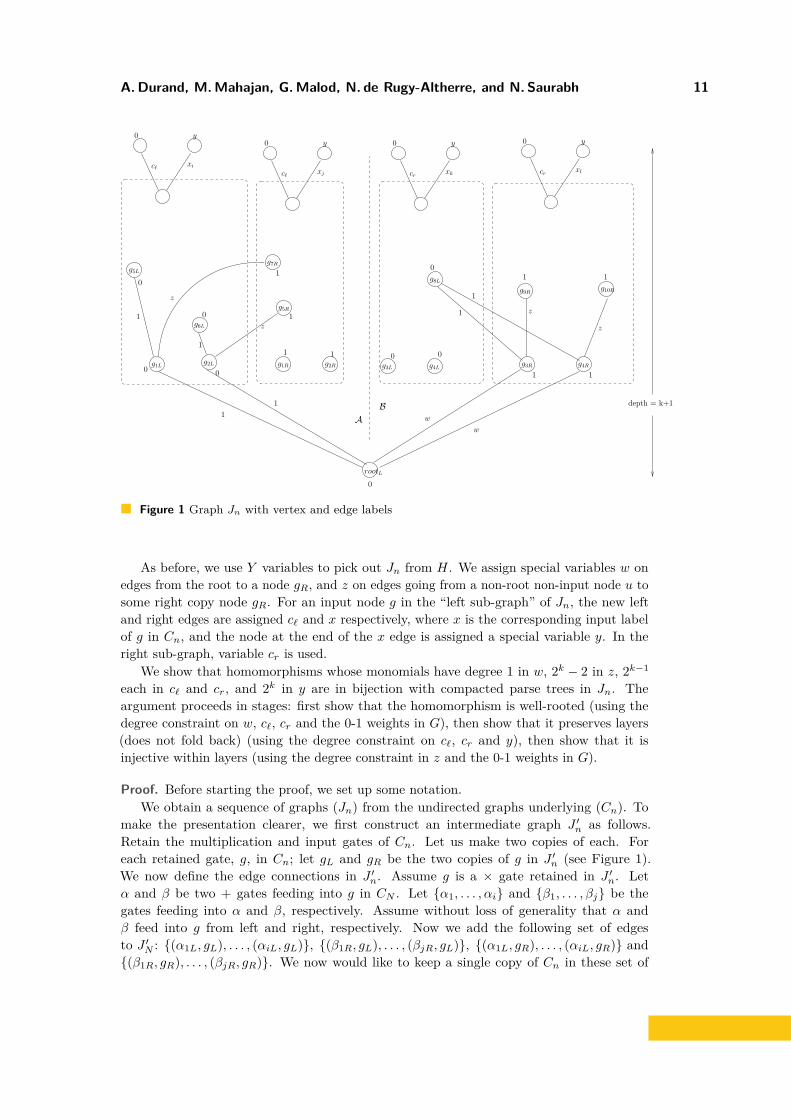
Figure 1 Graph Jn with vertex and edge labels

As before, we use Y variables to pick out Jn from H. We assign special variables w onedges from the root to a node gR, and z on edges going from a non-root non-input node u tosome right copy node gR. For an input node g in the “left sub-graph” of Jn, the new leftand right edges are assigned c` and x respectively, where x is the corresponding input labelof g in Cn, and the node at the end of the x edge is assigned a special variable y. In theright sub-graph, variable cr is used.

We show that homomorphisms whose monomials have degree 1 in w, 2k − 2 in z, 2k−1

each in c` and cr, and 2k in y are in bijection with compacted parse trees in Jn. Theargument proceeds in stages: first show that the homomorphism is well-rooted (using thedegree constraint on w, c`, cr and the 0-1 weights in G), then show that it preserves layers(does not fold back) (using the degree constraint on c`, cr and y), then show that it isinjective within layers (using the degree constraint in z and the 0-1 weights in G).

Proof. Before starting the proof, we set up some notation.We obtain a sequence of graphs (Jn) from the undirected graphs underlying (Cn). To

make the presentation clearer, we first construct an intermediate graph J ′n as follows.Retain the multiplication and input gates of Cn. Let us make two copies of each. Foreach retained gate, g, in Cn; let gL and gR be the two copies of g in J ′n (see Figure 1).We now define the edge connections in J ′n. Assume g is a × gate retained in J ′n. Letα and β be two + gates feeding into g in CN . Let {α1, . . . , αi} and {β1, . . . , βj} be thegates feeding into α and β, respectively. Assume without loss of generality that α andβ feed into g from left and right, respectively. Now we add the following set of edgesto J ′N : {(α1L, gL), . . . , (αiL, gL)}, {(β1R, gL), . . . , (βjR, gL)}, {(α1L, gR), . . . , (αiL, gR)} and{(β1R, gR), . . . , (βjR, gR)}. We now would like to keep a single copy of Cn in these set of


edges. So we remove the vertex rootR and we remove the remaining spurious edges infollowing way. If we assume that all edges are directed from root towards leaves, then wekeep only edges induced by the vertices reachable from rootL in this directed graph.

We now transform J ′n as follows to get Jn (see Figure 1): for each gate g′ in J ′n whichcorresponds to an input gate in Cn, we add two new distinct vertices and connect them tog′. Note that there are two type of vertices in Jn; one that corresponds to a gate in Cn andothers are degree 1 vertices hanging from gates that correspond to input gates in Cn.

I Observation 17. There is a one-to-one correspondence between parse trees of Cn andsubgraph of Jn that are rooted at rootL and isomorphic to T2k(n)+1 .

Let us set m := 2k(n)+1. The choice of poly(m) is such that 4sn ≤ poly(m). The Yvariables are set to {0, 1, w, z, c`, cr, x} such that the ones set to non-zero together form thegraph Jn. The X variables take values in {0, 1, y}. The ones corresponding to the left copiesof gates in Cn are set to 0, whereas to the right copies are set to 1. X variables for degree 1vertices hanging from input gates are set to 0 or ‘y’ depending on whether they are left orright child, respectively.

For every edge (rootL, gR), we set Y(rootL,gR) := w. For all u ∈ V (Jn), except rootL, anddegree of u not equal to 1, if the edge (u, gR) exist then we set Y(u,gR) := z.

Let v be a gate, in Jn, corresponding to an input gate g in Cn and v lies in A part (seeFigure 1). Let v1 and v2 be the left and right leaf attached to v, then we set Yvv1 := c` andYvv2 := the x-label of g in Cn.

For v a gate, in Jn, corresponding to an input gate g in Cn and lying in B part (seeFigure 1), let v1 and v2 be the left and right leaf attached to v. Then we set Yvv1 := cr andYvv2 := the x-label of g in Cn.

All other remaining edge variables that are not set to 0, are set to 1.By Observation 17 we easily deduce that for each parse tree p-T of Cn there ex-

ist a homomorphism φ from T2k(n)+1 to Jn such that mon(φ) is equal to mon(p-T) ×wz(2k−2)c2(k−1)

` c2(k−1)

r y2k , where k = k(n).We claim that for a homomorphism φ, if mon(φ) has degree 1 in w, (2k − 2) in z, 2k−1 in

c`, 2k−1 in cr and 2k in y, then the homomorphic image φ(T2k(n)+1) is isomorphic to T2k(n)+1

rooted at rootL.We will prove the claim in two parts. First we prove that if any node other than the root

of T2k(n)+1 is mapped to rootL then the corresponding monomial do not have right degree inw, c` or cr. We then consider the case where the root of the complete binary tree is the onlynode mapped to rootL under φ, and we argue that if φ has the required degrees then it mustbe a complete binary tree with 2k(n)+1 leaves rooted at rootL.

Case 1: φ−1(rootL) = ∅. Clearly mon(φ) has degree zero in w.Case 2: φ−1(rootL) contains a degree 3 vertex, say v. Let v1 and v2 be the left and

right child of v, respectively. Let v3 be the parent of v in Tm. Note that v must be labeled 0for the monomial to survive. Also, at least one of the vi’s is labeled 1.

Case 2a: Suppose two of the vi’s are labeled 1. Hence for the mon(φ) to survive thesevi’s must be mapped to the right of rootL. But then mon(φ) has degree at least 2 in w.

Case 2b: Exactly one of the vi is labeled 1. It must be the right child v2, for themonomial to survive it should be mapped to the right of rootL. Now if v1 or v3 is alsomapped to the right of rootL, mon(φ) will have degree at least 2 in w. Otherwise, both v1and v3 are mapped to the left of rootL. Since v1 is an internal vertex of Tm, the subtreerooted at v2 and v1 has depth at most k − 1 in Tm. In the first case mon(φ) does not havesufficient degree in c` , whereas in the second case it does not have sufficient degree in cr.


Case 3: φ−1(rootL) contains the root of Tm and at least one degree 1 vertex, say v.Also, no degree 3 vertices are mapped to rootL. As before, the left child of the root of Tm ismapped to the left of rootL and the right child is mapped to the right of rootL, else eitherthe monomial evaluates to zero or has degree at least 2 in w.

Case 3a: For some leaf node v mapped to rootL, its neighbour is mapped to the right ofrootL. In this case if the monomial is not zero, we will have at least degree 2 in w.

Case 3b: For all leaf node v mapped to rootL, their neighbour is mapped to the left ofrootL. But now mon(φ) will not have sufficient degree in c`.

Case 4: φ−1(rootL) contains only degree 1 vertices. But then the homomorphic imageis confined only to the left side or right side of rootL. Hence the monomial will not havesufficient degree in either cr or c`.

Therefore, we have shown that to get the appropriate degrees as claimed, φ−1(rootL)must only contain the root of Tm. Now to complete the proof we will show that if mon(φ)has correct degrees in w, z, c`, cr and y, then φ is injective and preserves left-right labellingof nodes of Tm. Note that for the monomial to survive and have degree 1 in w, it must bethe case that the right child of the root of Tm is mapped to the right of rootL and the leftchild is mapped to the left of rootL.

We claim that the homomorphism φ can not ‘fold back’ layers, that is, map a descendantto the node where its ancestor is mapped. This is because otherwise the monomial will nothave sufficient degree in either c`, cr, or y (if folding happens at depth k+1).

We also claim that the homomorphism φ can not ‘squish’ a layer, that is, map two siblingsto the same node. If the two are mapped to a vertex labeled 0, the monomial evaluates tozero. In the other case, they are mapped to a vertex labeled 1 but then the two siblingstogether, either contribute degree 2 in z or miss out at least degree 1 in c’s which cannot becompensated further if the monomial is non-zero.

Therefore we have shown that homomorphisms that are injective, whose image is iso-morphic to Tm and rooted at rootL, and which preserve left-right labels are in one-to-onecorrespondence with parse trees of Cn.

As before, to compute the universal polynomial we do an interpolation over the oraclepolynomial (Lemma 4) to extract the coefficient of wz(2k−2)c2(k−1)

` c2(k−1)

r y2k .J

4 Upper Bounds: membership in VP

In this section we will show that most of the variants of the homomorphism polynomialconsidered in the previous section are also computable by polynomial size arithmetic circuits.That is, the homomorphism polynomials are VP-Complete. For sake of clarity we describethe membership of a generic homomorphism polynomial in VP in detail. Then we explainhow to obtain various instantiations via projections.

We define a set of new variables Z := {Zu,a | u ∈ V (G) and a ∈ V (H)}. Let us generalisethe homomorphism polynomial fG,H,α,H as follows:

fG,H,H(Z, Y ) =∑φ∈H

∏u∈V (G)

Zu,φ(u)

∏(u,v)∈E(G)

Yφ(u),φ(v)

.

Note that for a 0-1 valued α, we can easily obtain fG,H,α,H from our generic homomorphismpolynomial fG,H,H via substitution of Z variables, setting Zu,a to Xα(u)

a . (If α can take anynon-negative values, then we can still do the above substitution. We will need subcircuits


computing appropriate powers of the X variables. The resulting circuit will still be poly-sizedand hence in VP, provided the powers are not too large.)

I Theorem 18. The family of homomorphism polynomials (fm) = fGm,Hm,Hom(Z, Y ) whereGm is Tm, the complete balanced binary tree with m = 2k leaves,Hm is Kn, complete graph on n = poly(m) nodes,

is in VP.

Proof. The idea is to group the homomorphisms based on where they send the root ofGm and its children, and to recursively compute sub-polynomials within each group. Thesub-polynomials in a specific group will have a specific set of variables in all their monomials.Thus the group can be identified by suitably combining partial derivatives of the recursivelyconstructed sub-polynomials. (Note: this is why we consider the generalised polynomial withZ instead of X and α. If for some u, α(u) = 0, then we cannot use partial derivatives to forcesending u to a specific vertex of H.) The partial derivatives themselves can be computedefficiently using Lemma 3.

We show by induction on m that f = fm can be computed in size S(m,n) = O(m3n3).In the base case when m = 1, f =

∑a∈V (H) Zu,a, and the trivial circuit is of size n.

For m ≥ 2, let r, r1, r2 denote the root of T = Gm and its two children. Then T is thedisjoint union of the node r, the edges (r, r1) and (r, r2), and the two trees T1 and T2 rootedat r1, r2 respectively. Note that a homomorphism can be decomposed on these subtrees andvice versa. i.e.,

{φ ∈ Hom | φ : T → H} ={a ◦ φ1 ◦ φ2 |

a ∈ V (H), φi : Ti → H, φi ∈ Hom, and(φ1 (r1) , a) , (φ2 (r2) , a) ∈ E(H)

}This allows us to construct the polynomial recursively.

f =∑

φ:T→Hmon(φ) =

∑h∈V (H)

φ1:T1→H∈Homφ2:T2→H∈Hom

(φ1(r1),h),(φ2(r2),h)∈E(H)

mon(h ◦ φ1 ◦ φ2)

=∑

h,h1,h2∈V (H)(h,h1),(h,h2)∈E(H)

∑φ1:T1→Hφ1(r1)=h1

∑φ2:T2→Hφ1(r2)=h2

Zr,hYh,h1Yh,h2mon(φ1)mon(φ2)

=∑

h,h1,h2∈V (H)(h,h1),(h,h2)∈E(H)

Zr,hYh,h1Yh,h2

∑φ1:T1→Hφ1(r1)=h1

mon(φ1)

∑φ2:T2→Hφ1(r2)=h2

mon(φ2)

=

∑h,h1,h2∈V (H)

(h,h1),(h,h2)∈E(H)

Zr,hYh,h1Yh,h2

(Zr1,h1

∂fT1,H,Hom∂Zr1,h1

)(Zr2,h2

∂fT2,H,Hom∂Zv2,h2

)

By induction, we have two circuits of size S(m2 , n) each, computing fT1,H,Hom andfT2,H,Hom respectively. Using Lemma 3, we have a circuit of size 6S(m2 , n) computingboth these sub-polynomials and all their derivatives. Thus we can construct f in size6S(m2 , n) +O(n3), giving the result. J

I Remark. In the above theorem and proof, if Gm is ATum instead of Tm, essentially thesame construction works. The grouping of homomorphisms should be based on the imagesof the root and its children and grandchildren as well.


If Gm and Hm have directions, again everything goes through the same way.If we want to consider a restricted set H of homomorphisms DirHom or ColHom

instead of all of Hom, again the same construction works. All we need is that H can bedecomposed into independent parts with a local stitching-together operator. That is, whetherφ belongs to H can be verified locally edge-by-edge and/or vertex-by-vertex, so that this canbe built into the decomposition and the recursive construction.

From Theorem 18, the discussion preceding it and the remark following it, we have:

I Corollary 19. The polynomial families from Proposition 12, Theorems 14, 15, and 16 areall in VP.

I Remark. It is not clear how to get a similar upper bound for InjDirHom when the targetgraph is the complete directed graph (remark following Proposition 12), or for the familyfrom Proposition 13. We need a way of enforcing that the recursive construction aboverespects injectivity. This is not a problem for Proposition 12, though, because there thetarget graph is the graph underlying a multiplicatively disjoint circuit. Injectivity at theroot and its children and grandchildren can be checked locally; the recursion beyond thatdoes not fold back because the homomorphisms are direction-preserving. The constructionmay not work if the target graph is the complete directed graph.

From Corollary 19, Proposition 12, and Theorems 14, 15 and 16, we obtain our mainresult:

I Theorem 20. 1. The polynomial families from Proposition 12 and Theorem 15 are com-plete for VP with respect to p-projections.

2. The polynomial families from Theorems 14 and 16 are complete for VP with respect toconstant-depth c-reductions.

5 Characterizing other complexity classes

We complement our result of VP-completeness by showing that appropriate modification ofG can lead to VBP-complete and VNP-complete polynomial families.

VBP CompletenessVBP is the class of polynomials computed by polynomial-sized algebraic branching programs.These are layered directed graphs, with edges labeled by field constants or variables, and witha designated source node s and target node t. For any path ρ in G, the monomial mon(ρ)is the product of the labels of all edges in ρ. For two nodes u, v, the polynomial puv sumsmon(ρ) for all paths ρ from u to v. The branching program computes the polynomial pst.

A well-known polynomial family complete for VBP is the determinant of a generic matrix.A generic complete polynomial for VBP is the polynomial computed by an ABP with (1) asource node s, m − 1 layers of m nodes each, and a target node t, (2) complete bipartitegraphs between layers, and (3) distinct variables x on all edges. This is also the iteratedmatrix multiplication polynomial IMM. It is easy to see that st paths play the same rolehere as parse trees did in the multiplicatively disjoint circuits.

I Theorem 21. Consider the homomorphism polynomial whereG is a simple path on m+ 1 nodes, (u1, u2, . . . , um+1).H is a complete graph (undirected) on m2 nodes.H := set of all homomorphisms from G to H.


Define α such that,

α(u) ={

1 u = u1 or u = um+10 otherwise

Then, the family (fG,H,α,Hom(X, Y ))m, where m ∈ N, is complete for VBP under c-reductions.

Proof. Hardness: We show how IMM can be computed from this polynomial. Set the Yvariables to 0 or to variables from x so that H looks like the undirected graph underlyingthe generic ABP. Set the X variables to 0, except at the nodes S, T corresponding to s, t.Note that in the resulting graph H ′, the shortest path between S and T has exactly m edges.Though there are no directions, the bijection between {S, T} and {s, t} is established by thesetting of the Y variables.

For every st path ρ in the ABP, there is a homomorphism φ from G to H such thatmon(φ) = Xsmon(ρ)XT . Conversely, for any homomorphism φ from G to H, if mon(φ)contains XSXT , then φ must map G to a proper path between S, T . So mon(φ)/XSXT is infact mon(ρ) for some st path ρ. Hence the homogeneous component of fG,H,α,Hom of degree1 in XS and degree 1 in XT is exactly the generic IMM polynomial.

Membership: We show that more generally, for G,H,H as defined and for any 0-1valued α, the polynomial can be computed in VBP. For any non-negative n,m, let qn,mdenote the generalised homomorphism polynomial fPn,Km,Hom(Z, Y ) as defined in Section 4.(The polynomial in the Theorem statement, fPm,Km2 ,α,Hom, is obtained from qm,m2 bysetting Zu,a to Xα(u)

a .) Let us see the construction of an ABP computing qn,m. We describeit in detail for q2,m; it generalizes in a straightforward way to all n. Let P2 = 〈u, v, w〉 be apath of length 2, with edges (u, v) and (v, w). We will demonstrate the ABP constructionby reducing the polynomial computation to an iterated matrix multiplication instance. Weneed the following easily-verifiable fact.

I Fact 22. Graph homomorphisms from a path of length ‘n’ to any graph H are in one-to-onecorrespondence with walks of length exactly ‘n’ in graph H.

We claim that q2,m equals the following matrix product,

11...1

T

Zu,1Y1,1 Zu,1Y1,2 · · · Zu,1Y1,mZu,2Y2,1 Zu,2Y2,2 · · · Zu,2Y2,m

......

. . ....

Zu,mYm,1 Zu,mYm,2 · · · Zu,mYm,m

Zv,1Y1,1 Zv,1Y1,2 · · · Zv,1Y1,mZv,2Y2,1 Zv,2Y2,2 · · · Zv,2Y2,m

......

. . ....

Zv,mYm,1 Zv,mYm,2 · · · Zv,mYm,m

Zw,1Zw,2...

Zw,m

A typical entry in the final polynomial is Zu,iYi,j×Zv,jYj,k×Zw,k. The initial row vector

is only used for summation over i. So let us focus on the adjacency matrix of Km, whereeach entry is multiplied with a suitable Z variable. Intuitively, the first matrix picks a vertexi in Km to match u, and then also picks an edge (i, j) from i to map the edge (u, v) in thepath. The second matrix then picks the Z variable for v, j, and chooses an edge (j, k) tomap (v, w). The last column vector just picks the Z variable for w, k, as there are no moreedges left. J

We now proceed to provide variants of path homomorphism polynomial that are completefor VBP under projections. Unfortunately, this strong completeness result comes with acaveat. The graphs underlying the homomorphism polynomials are now directed graphs.But we believe that the restriction is not a severe one (compare it with Theorem 14).


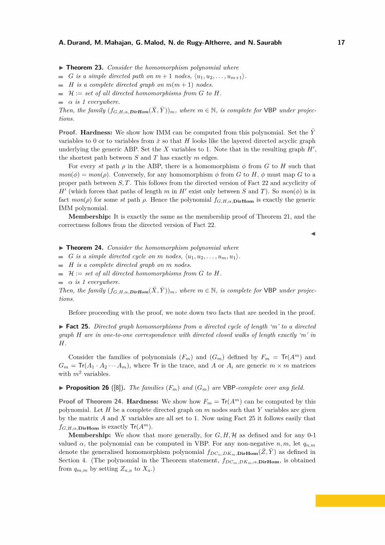
I Theorem 23. Consider the homomorphism polynomial whereG is a simple directed path on m+ 1 nodes, 〈u1, u2, . . . , um+1〉.H is a complete directed graph on m(m+ 1) nodes.H := set of all directed homomorphisms from G to H.α is 1 everywhere.

Then, the family (fG,H,α,DirHom(X, Y ))m, where m ∈ N, is complete for VBP under projec-tions.

Proof. Hardness: We show how IMM can be computed from this polynomial. Set the Yvariables to 0 or to variables from x so that H looks like the layered directed acyclic graphunderlying the generic ABP. Set the X variables to 1. Note that in the resulting graph H ′,the shortest path between S and T has exactly m edges.

For every st path ρ in the ABP, there is a homomorphism φ from G to H such thatmon(φ) = mon(ρ). Conversely, for any homomorphism φ from G to H, φ must map G to aproper path between S, T . This follows from the directed version of Fact 22 and acyclicity ofH ′ (which forces that paths of length m in H ′ exist only between S and T ). So mon(φ) is infact mon(ρ) for some st path ρ. Hence the polynomial fG,H,α,DirHom is exactly the genericIMM polynomial.

Membership: It is exactly the same as the membership proof of Theorem 21, and thecorrectness follows from the directed version of Fact 22.

J

I Theorem 24. Consider the homomorphism polynomial whereG is a simple directed cycle on m nodes, 〈u1, u2, . . . , um, u1〉.H is a complete directed graph on m nodes.H := set of all directed homomorphisms from G to H.α is 1 everywhere.

Then, the family (fG,H,α,DirHom(X, Y ))m, where m ∈ N, is complete for VBP under projec-tions.

Before proceeding with the proof, we note down two facts that are needed in the proof.

I Fact 25. Directed graph homomorphisms from a directed cycle of length ‘m’ to a directedgraph H are in one-to-one correspondence with directed closed walks of length exactly ‘m’ inH.

Consider the families of polynomials (Fm) and (Gm) defined by Fm = Tr(Am) andGm = Tr(A1 · A2 · · ·Am), where Tr is the trace, and A or Ai are generic m ×m matriceswith m2 variables.

I Proposition 26 ([8]). The families (Fm) and (Gm) are VBP-complete over any field.

Proof of Theorem 24. Hardness: We show how Fm = Tr(Am) can be computed by thispolynomial. Let H be a complete directed graph on m nodes such that Y variables are givenby the matrix A and X variables are all set to 1. Now using Fact 25 it follows easily thatfG,H,α,DirHom is exactly Tr(Am).

Membership: We show that more generally, for G,H,H as defined and for any 0-1valued α, the polynomial can be computed in VBP. For any non-negative n,m, let qn,mdenote the generalised homomorphism polynomial fDCn,DKm,DirHom(Z, Y ) as defined inSection 4. (The polynomial in the Theorem statement, fDCm,DKm,α,DirHom, is obtainedfrom qm,m by setting Zu,a to Xa.)


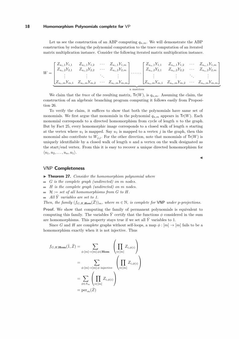
Let us see the construction of an ABP computing qn,m. We will demonstrate the ABPconstruction by reducing the polynomial computation to the trace computation of an iteratedmatrix multiplication instance. Consider the following iterated matrix multiplication instance.

W =

Zu1,1Y1,1 Zu1,1Y1,2 · · · Zu1,1Y1,mZu1,2Y2,1 Zu1,2Y2,2 · · · Zu1,2Y2,m

......

. . ....

Zu1,mYm,1 Zu1,mYm,2 · · · Zu1,mYm,m

· · · · · ·Zun,1Y1,1 Zun,1Y1,2 · · · Zun,1Y1,mZun,2Y2,1 Zun,2Y2,2 · · · Zun,2Y2,m

......

. . ....

Zun,mYm,1 Zun,mYm,2 · · · Zun,mYm,m

︸︷︷︸

n matrices

We claim that the trace of the resulting matrix, Tr(W ), is qn,m. Assuming the claim, theconstruction of an algebraic branching program computing it follows easily from Proposi-tion 26.

To verify the claim, it suffices to show that both the polynomials have same set ofmonomials. We first argue that monomials in the polynomial qn,m appears in Tr(W ). Eachmonomial corresponds to a directed homomorphism from cycle of length n to the graph.But by Fact 25, every homomorphic image corresponds to a closed walk of length n startingat the vertex where u1 is mapped. Say u1 is mapped to a vertex j in the graph, then thismonomial also contribute to Wj,j . For the other direction, note that monomials of Tr(W ) isuniquely identifiable by a closed walk of length n and a vertex on the walk designated asthe start/end vertex. From this it is easy to recover a unique directed homomorphism for〈u1, u2, . . . , un, u1〉.

J

VNP CompletenessI Theorem 27. Consider the homomorphism polynomial where

G is the complete graph (undirected) on m nodes.H is the complete graph (undirected) on m nodes.H := set of all homomorphisms from G to H.All Y variables are set to 1.

Then, the family (fG,H,Hom(Z))m, where m ∈ N, is complete for VNP under p-projections.

Proof. We show that computing the family of permanent polynomials is equivalent tocomputing this family. The variables Y certify that the functions φ considered in the sumare homomorphisms. This property stays true if we set all Y variables to 1.

Since G and H are complete graphs without self-loops, a map φ : [m]→ [m] fails to be ahomomorphism exactly when it is not injective. Thus

fG,H,Hom(1, Z) =∑

φ:[m]→[m];φ∈Hom

∏i∈[m]

Zi,φ(i)

=

∑φ:[m]→[m];φ injective

∏i∈[m]

Zi,φ(i)

=∑φ∈Sm

∏i∈[m]

Zi,φ(i)

= perm(Z)


Thus fG,H,Hom is exactly the perm polynomial, and hence is complete for VNP.J

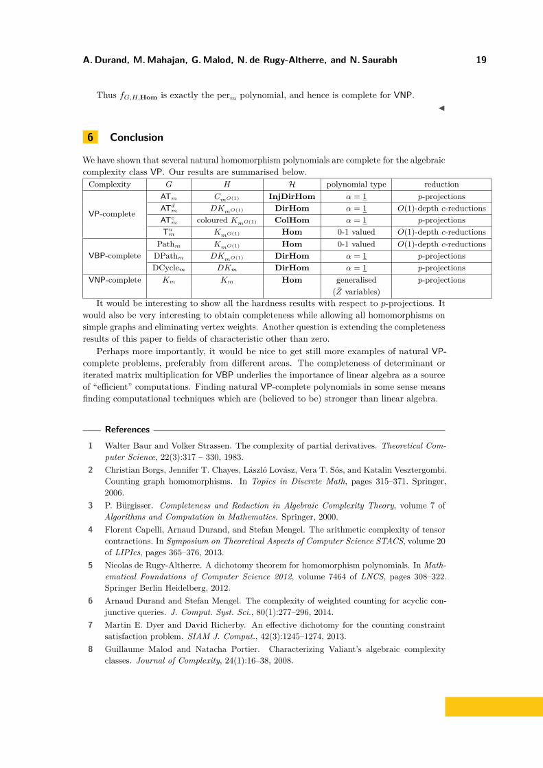
6 Conclusion

We have shown that several natural homomorphism polynomials are complete for the algebraiccomplexity class VP. Our results are summarised below.

Complexity G H H polynomial type reduction

VP-complete

ATm CmO(1) InjDirHom α = 1 p-projectionsATd

m DKmO(1) DirHom α = 1 O(1)-depth c-reductionsATc

m coloured KmO(1) ColHom α = 1 p-projectionsTu

m KmO(1) Hom 0-1 valued O(1)-depth c-reductions

VBP-completePathm KmO(1) Hom 0-1 valued O(1)-depth c-reductions

DPathm DKmO(1) DirHom α = 1 p-projectionsDCyclem DKm DirHom α = 1 p-projections

VNP-complete Km Km Hom generalised p-projections(Z variables)

It would be interesting to show all the hardness results with respect to p-projections. Itwould also be very interesting to obtain completeness while allowing all homomorphisms onsimple graphs and eliminating vertex weights. Another question is extending the completenessresults of this paper to fields of characteristic other than zero.

Perhaps more importantly, it would be nice to get still more examples of natural VP-complete problems, preferably from different areas. The completeness of determinant oriterated matrix multiplication for VBP underlies the importance of linear algebra as a sourceof “efficient” computations. Finding natural VP-complete polynomials in some sense meansfinding computational techniques which are (believed to be) stronger than linear algebra.

References

1 Walter Baur and Volker Strassen. The complexity of partial derivatives. Theoretical Com-puter Science, 22(3):317 – 330, 1983.

2 Christian Borgs, Jennifer T. Chayes, László Lovász, Vera T. Sós, and Katalin Vesztergombi.Counting graph homomorphisms. In Topics in Discrete Math, pages 315–371. Springer,2006.

3 P. Bürgisser. Completeness and Reduction in Algebraic Complexity Theory, volume 7 ofAlgorithms and Computation in Mathematics. Springer, 2000.

4 Florent Capelli, Arnaud Durand, and Stefan Mengel. The arithmetic complexity of tensorcontractions. In Symposium on Theoretical Aspects of Computer Science STACS, volume 20of LIPIcs, pages 365–376, 2013.

5 Nicolas de Rugy-Altherre. A dichotomy theorem for homomorphism polynomials. In Math-ematical Foundations of Computer Science 2012, volume 7464 of LNCS, pages 308–322.Springer Berlin Heidelberg, 2012.

6 Arnaud Durand and Stefan Mengel. The complexity of weighted counting for acyclic con-junctive queries. J. Comput. Syst. Sci., 80(1):277–296, 2014.

7 Martin E. Dyer and David Richerby. An effective dichotomy for the counting constraintsatisfaction problem. SIAM J. Comput., 42(3):1245–1274, 2013.

8 Guillaume Malod and Natacha Portier. Characterizing Valiant’s algebraic complexityclasses. Journal of Complexity, 24(1):16–38, 2008.


9 Stefan Mengel. Characterizing arithmetic circuit classes by constraint satisfaction problems.In Automata, Languages and Programming, volume 6755 of LNCS, pages 700–711. SpringerBerlin Heidelberg, 2011.

10 Ran Raz. Elusive functions and lower bounds for arithmetic circuits. Theory of Computing,6:135–177, 2010.

11 Amir Shpilka and Amir Yehudayoff. Arithmetic circuits: A survey of recent results andopen questions. Foundations and Trends in Theoretical Computer Science, 5(3-4):207–388,2010.

12 L. G. Valiant. Reducibility by algebraic projections. In Logic and Algorithmic: InternationalSymposium in honour of Ernst Specker, volume 30, pages 365–380. Monograph. de l’Enseign.Math., 1982.

13 Leslie G. Valiant. Completeness classes in algebra. In Symposium on Theory of ComputingSTOC, pages 249–261, 1979.

14 Leslie G. Valiant, Sven Skyum, S. Berkowitz, and Charles Rackoff. Fast parallel compu-tation of polynomials using few processors. SIAM Journal on Computing, 12(4):641–644,1983.

ECCC ISSN 1433-8092

http://eccc.hpi-web.de

Electronic Colloquium on ... - logique.jussieu.frnderugy/doc/VPCompletECCC.pdfElectronic Colloquium...

Documents

Transcript of Electronic Colloquium on ... - logique.jussieu.frnderugy/doc/VPCompletECCC.pdfElectronic Colloquium...