ELECTROMAGNETIC THEORY

AND

TRANSMISSION LINES

Prepared By

Mrs. A.Usha Rani

Associate Professor

and

Mr. G. Nagendra Prasad

Associate Professor

1/24/2018

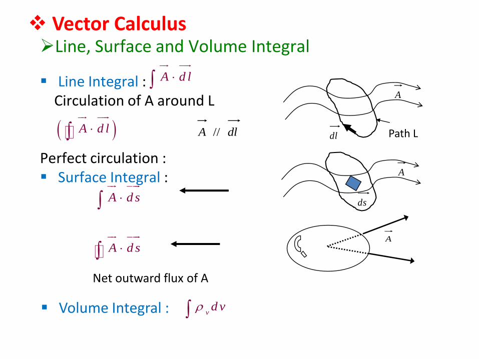
Line, Surface and Volume Integral

Line Integral : Circulation of A around L

Perfect circulation : Surface Integral :

dl

A

Path LdlA //

A d s

ds

A

A

A d s

Net outward flux of A

A d l

A d l

Volume Integral : vd v

Vector Calculus

Del operator:

Gradient :

Divergence :

Curl:

Laplacian of scalar :

a x a y a zx y z

:V V V

V V a x a y a zx y z

: ( )A x A y A z

A Ax y z

: ( ) ( ) ( )A z A y A x A z A y A x

A A a x a y a zy z y x x y

2 2 2

2

2 2 2: ( )

V V VV V

x y z

1/24/2018

Divergence, Gaussian’s law

lim

0

A d s

d iv A Av v

It is a scalar field

sink:0

source:0

A

A

: 'A d s

fro m th e eq u a tio n

G a u s s ia n s th eA yd v o r

Curl, Stoke’s theorem

lim

0

A d l

C u r l A As s

0)(.3

0)(.2

:.1

V

A

sensenomakesV

':A d

fro m th e eq u a tio n

S to ke s th eol A d s ry

ds

Closed path L

A

1/24/2018

UNIT-I

ELECTROSTATICS

1/24/2018

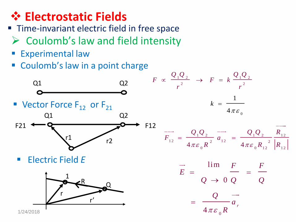
Coulomb’s law and field intensity Experimental law Coulomb’s law in a point charge

Q1 Q21 2

2

0

1 2

2

1

4

Q Q Q

k

QF F k

r r

Vector Force F12 or F21

r1 r2

F21

Q2Q1

F121 2 1 2 1 2

1 2 1 22 2

0 0 1 2 1 24 4

Q Q Q Q RF a

R R R

Electrostatic Fields Time-invariant electric field in free space

rr’

1QR

Electric Field E

0

lim

0

4r

F FE

Q Q Q

Qa

R

1/24/2018

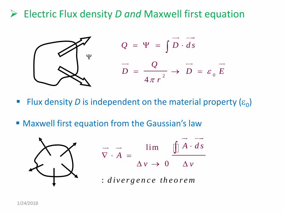
Electric Flux density D and Maxwell first equation

024

Q D d s

QD D E

r

Flux density D is independent on the material property (0)

Maxwell first equation from the Gaussian’s law

l

:

im

0

A d

d iv e rg

s

e n c e

Av

th e o r e m

v

1/24/2018

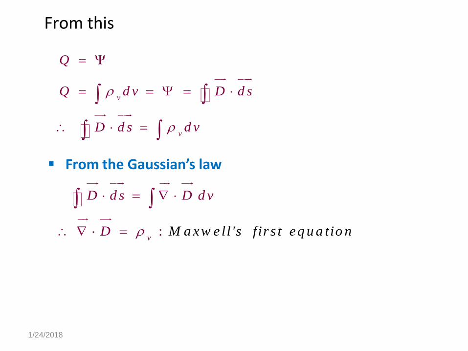
From this

v

v

Q

Q d v D d s

D d s d v

From the Gaussian’s law

:v

M a xw e ll 's fir s t eq u a tio n

D d s D d v

D

1/24/2018

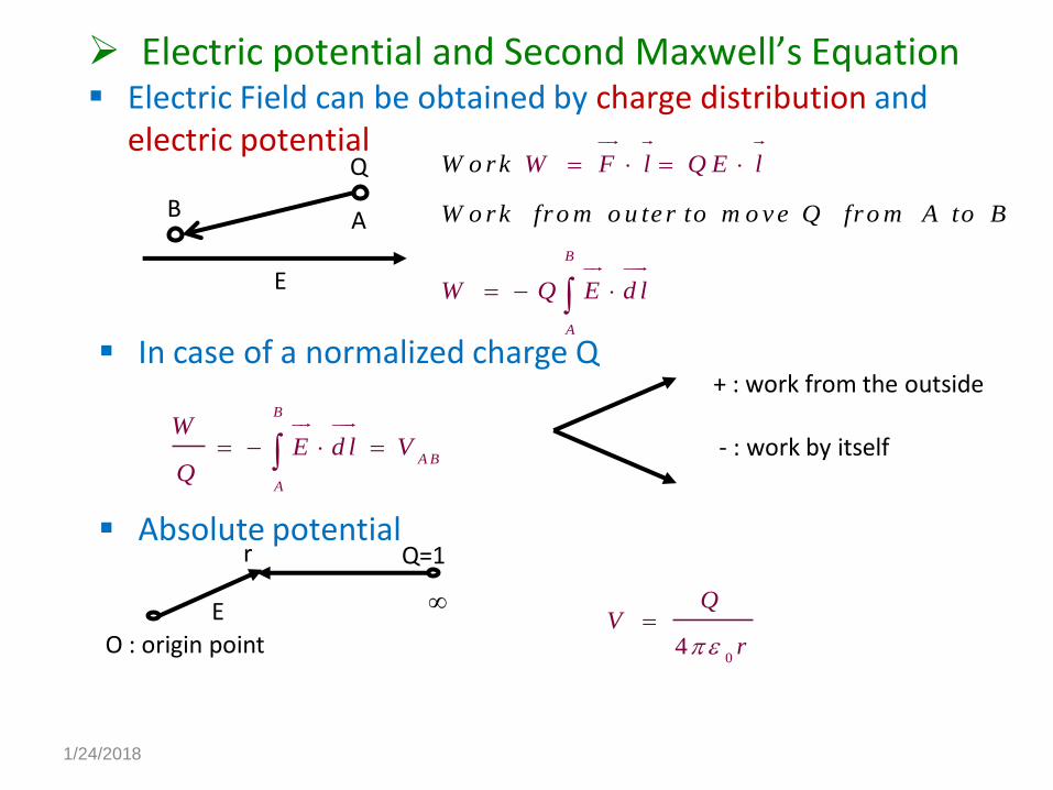
Electric potential and Second Maxwell’s Equation Electric Field can be obtained by charge distribution and

electric potential

E

A

Q

B

B

A

W o rk

W o rk fro m o u te r to m o ve Q fro m

W F l Q E l

W Q E

A to

d

B

l

In case of a normalized charge Q

B

A B

A

WE d l V

Q

+ : work from the outside

- : work by itself

E

r

O : origin point

Q=1

04

QV

r

Absolute potential

1/24/2018

Second Maxwell’s Equ. From E and V

:

)

0

'0 (

A B B A A B B A

B A

A B B A

A B

V V V V

V V E d

C ircu la t io n

S t

l E d l

E d l E o ke s th ed s o rem

Relationship between E and V

0E

( )

, ,

d V E d l E x d x E y d y E zd z

V V Vd x d y d z

x y z

V V VE x E y E z

x y z

E V

E3 4 5

3,4,5 : Equi-potential Line

1/24/2018

Energy density

1

2

1( )

2

1( )

2

1( )

2

vW e V d v

D V d v

D V d v

D E d v

E field in material space ( not free space)

MaterialConductor

Non conductor

Insulator

Dielctric material

Material can be classified by conductivity << 1 : insulator >> 1 : conductor (metal : )Middle range of : dielectric

1/24/2018

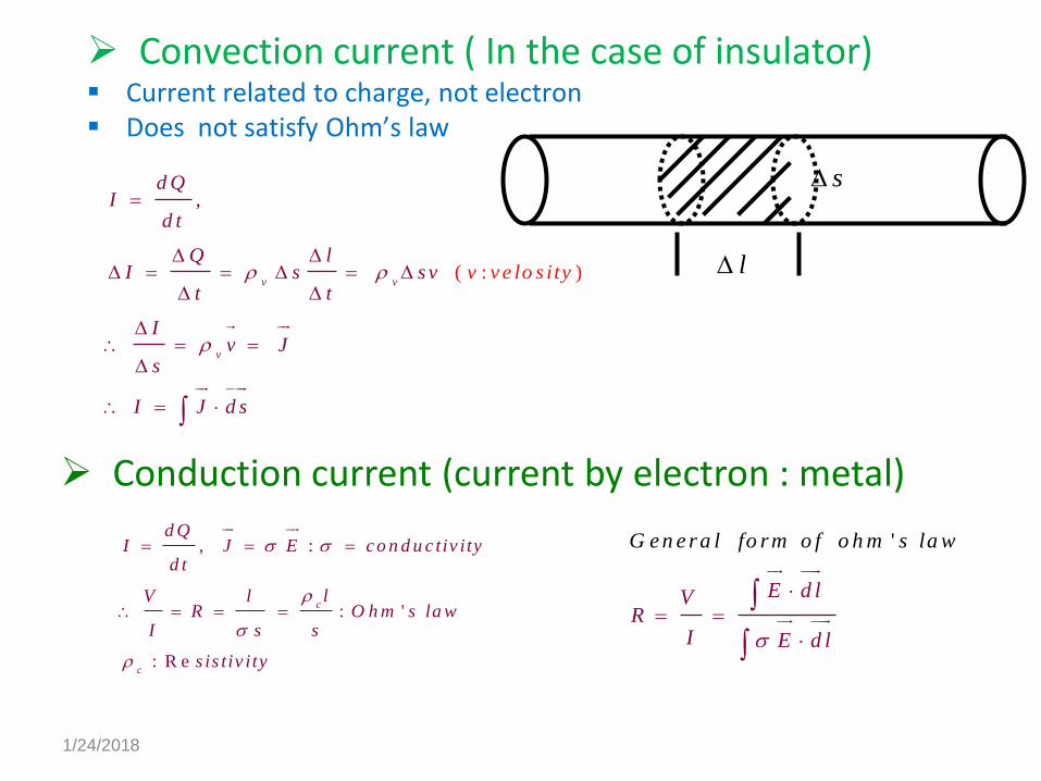
Convection current ( In the case of insulator) Current related to charge, not electron Does not satisfy Ohm’s law

l

s

( : )

,

v v

v

v v e lo s i ty

d QI

d t

Q lI s s v

t t

Iv J

s

I J d s

Conduction current (current by electron : metal)

, :

: '

: R e

c

c

d QI J E co n d u c tiv ity

d t

lV lR O h m s la w

I s s

s is t iv i ty

'

E d lV

G en e ra l fo rm o f o h m s la w

RI E d l

1/24/2018

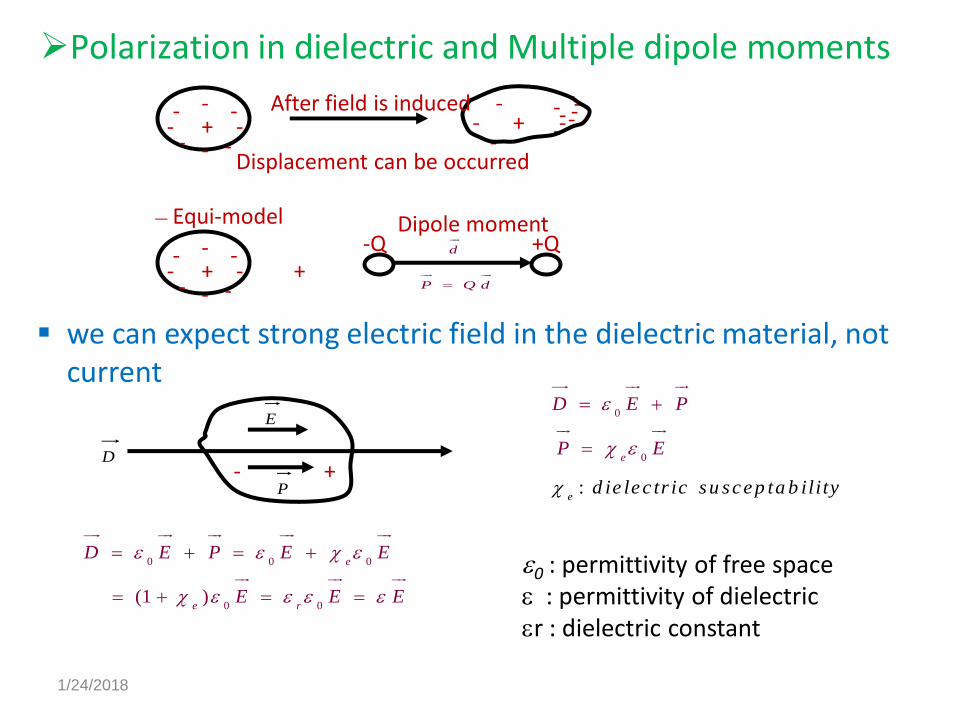
Polarization in dielectric and Multiple dipole moments

we can expect strong electric field in the dielectric material, not current

+-

---

-

-

-

- --

--

---

----

+After field is induced

Displacement can be occurred

– Equi-model

+-

---

-

-

-

-+

-Q +Qd

P Q d

Dipole moment

- +D

P

E0

0

:e

e

d ie

D

lec tr ic su scep t

E P

P E

a b ility

0 0 0

0 0(1 )

e

e r

D E P E E

E E E

0 : permittivity of free space : permittivity of dielectricr : dielectric constant

1/24/2018

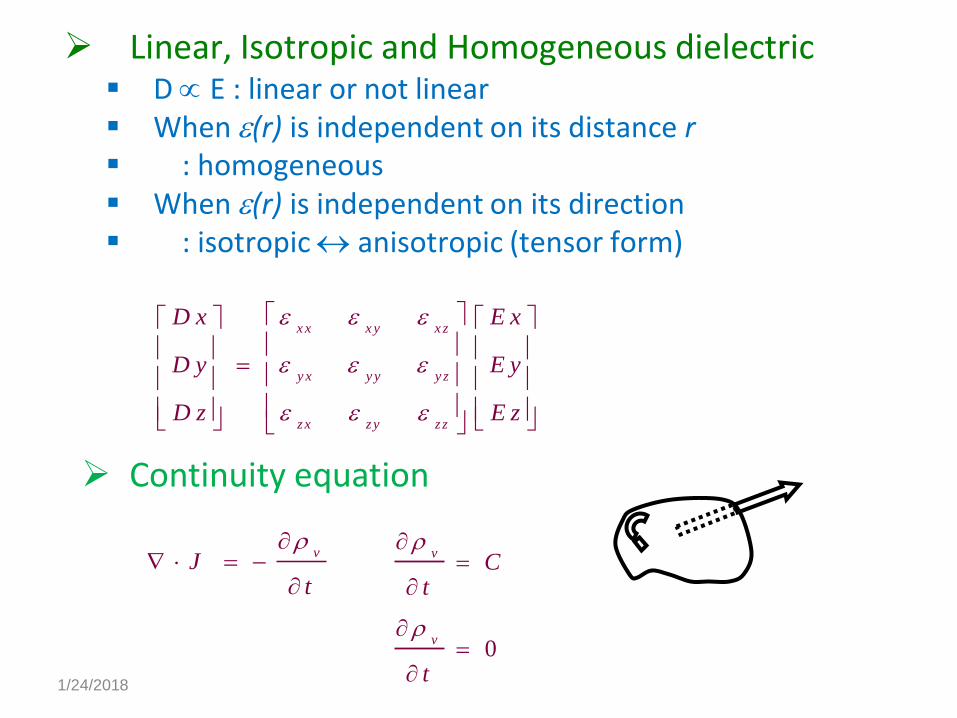
Linear, Isotropic and Homogeneous dielectric D E : linear or not linear When (r) is independent on its distance r : homogeneous When (r) is independent on its direction : isotropic anisotropic (tensor form)

x x x y x z

y x y y y z

zx zy z z

D x E x

D y E y

D z E z

Continuity equation

vJ

t

0

v

v

Ct

t

1/24/2018

Poisson eq. and Laplacian Practical solution for electrostatic field

2

2

( h o m o g e n e o u s )

( .)

,

)

(

0 (

)

0

v

v

v

i f

p o is s o n e q

if L a p la c ia n

h a rm o n ic so lu t io n

D E E V

V

V

V

Boundary condition

Dielectric to dielectric boundary Conductor to dielectric boundary Conductor to free space boundary

1/24/2018

UNIT-II

MAGNETOSTATICS

1/24/2018

Magnetostatics deals with the behaviour of stationaryMagnetic fields.

Oersterd and Ampere proved experimentally that thecurrent carrying conductor produces a magnetic field aroundit.

The origin of Magnetism is linked with current and magneticquantities are measured in terms of current.

Magnetic dipole Any two opposite magnetic poles separated by a

distance d constitute a magnetic dipole.

Magnetostatic Fields

1/24/2018

Bio-Savart’s law

I

dl

H fieldRandIbtwangle

R

lengthntdisplacemedl

currentI

:

distance:

:

:

2 34 4

rI d l a I d l R

d HR R

Experimental eq.

Independent on material property

R

The direction of dH is determined by right-hand rule Independent on material property

Current element is defined by

I

K

Idl (line current) Kds (surface current)Jdv (volume current)

1/24/2018

Ampere’s circuital law

I

H

dl

enc

IdlHI enc : enclosed by path

By applying the Stoke’s theorem

(

: '

)en c

H d l H d s I J d

M a x w e ll s th ird e q u a tio n

s

H J

Magnetic flux density

0

0

0

( )

( )

:

D e le c tro s ta tic fie ld

m a g n e to s ta tic fie ld

p e rm e a b ility

E

B H

2

:

( )

:

( / )

m a g n e tic flu x

w b

B m a g n e tic flu x d e n s ity

B d

m

s

w b

• Magnetic flux line always has same start and end point

1/24/2018

Maxwell’s eq. For static EM field

0

0

vD

B

E

H J

0

0

D

B

BE

t

DH

t

Time varient system

1/24/2018

Magnetic scalar and vector potentials

Efro m V

0

( ) 0

V

A

( ) 0

mH J V

Vm : magnetic scalar potential It is defined in the region that J=0

( ) 0A B

A : magnetic vector potential

Magnetic force

Q E eF Q E

Bu

Q

mF Q u B

Fm : dependent on charge velocitydoes not work (Fm dl = 0) only rotationdoes not make kinetic energy of charges change

1/24/2018

Lorentz force

Magnetic torque and moment

Current loop in the magnetic field H D.C motor, generator Loop//H max rotating power

)( BuEQBuQEQFFFme

an

B

F0

F0

` ( )

n

T r F m B N m

m IS a

1/24/2018

Magnetic dipole

A bar magnet or small current loop

I

m

N

S

m

A bar magnet A small current loop

Material in B field

B 0

0

0

( )

(1 )

:

m

m

r

B

p e rm e a b i

H H

H

li

H H

ty

1/24/2018

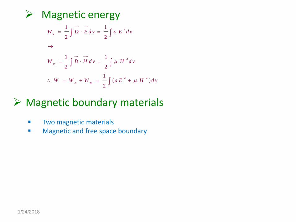
Magnetic energy2

2

2 2

1 1

2 2

1 1

2 2

1( )

2

e

m

e m

W D E d v E d v

W B H d v H d v

W W W E H d v

Magnetic boundary materials

Two magnetic materials Magnetic and free space boundary

1/24/2018

Maxwell equations In the static field, E and H are independent on each other,

but interdependent in the dynamic field Time-varying EM field : E(x,y,z,t), H(x,y,z,t) Time-varying EM field or waves : due to accelated charge

or time varying current

a rg

( . .)

v a r

E le c tro s ta tic fie ld s ta tic c h e

M a g n e to s ta tic fie ld s ta tic c u rre n t D C

E le c tro m a g n e tic fie ld tim e y in g c u rre n ts

1/24/2018

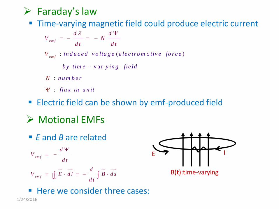
Faraday’s law Time-varying magnetic field could produce electric current

:

:

:

( )

v a r

e m

e f

f

m

in d u c e d v o lta g e e le c tro m o tiv e fo r c e

b y tim e y in g fie ld

n u m

d dV N

d

b e r

flu x in u n

t

V

d

it

N

t

Electric field can be shown by emf-produced field

Motional EMFs

E and B are related

e m f

e m f

dV

d t

dV E d l B d s

d t

B(t):time-varying

IE

Here we consider three cases:1/24/2018

Stationary loop, time-varying B field

( )

v: a r

e m f

d BV E d l B d s d s

d t t

BE d l E d s d s

M a x w e ll e q u a tio n tim e y in g fie ld

t

BE

tfo r

Time-varying loop and static B field

: o n a c h a rg e

: m o tio n a l e le c tr ic f ie ld

B y a p p ly in g s to k e 's th e o r

( ) ( )

(

e m

m

m

e m f m

m

m

m

m

F Q v B

FE m v B

Q

V E d l v B d l

E d l E d s v B

E v

E

d s

: M a x w e ll 's e q u a tio n fo r tim e -v a ry in g o p) l oB

1/24/2018

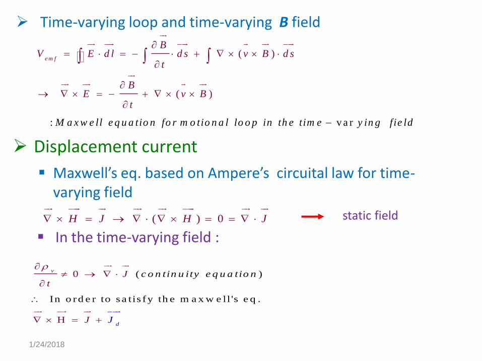
Time-varying loop and time-varying B field

: v a

(

r

)

( )

e m f

BV E d l d s v B d s

t

BE v B

t

M a x w e ll e q u a tio n fo r m o tio n a l lo o p in th e tim e y in g fie ld

Displacement current

Maxwell’s eq. based on Ampere’s circuital law for time-varying field

( ) 0H J H J

static field

( )

In o rd e r to s a tis fy th e m a x w e ll 's e q

0

H

.

d

vc o n tin u ity e q u aJ

t

J

tio n

J

In the time-varying field :

1/24/2018

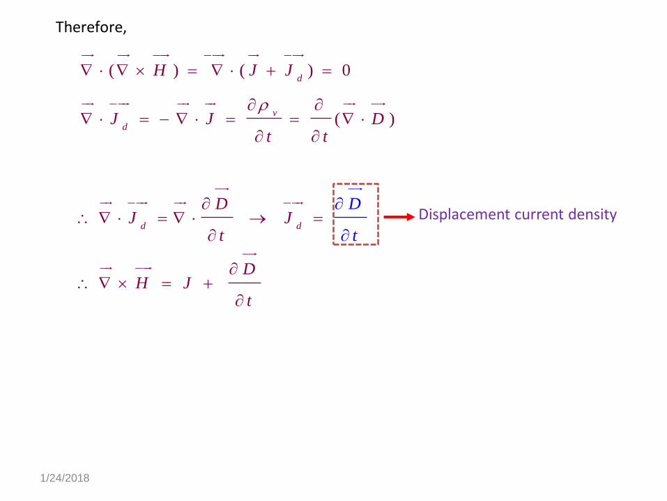
Therefore,

( ) ( ) 0

( )

d

v

d

d d

H J J

J J Dt t

DJ J

t

DH J

t

D

t

Displacement current density

1/24/2018

Maxwell’s Equations in final forms

0

vD

B

BE

t

DH J

t

0

( )

v

v

s

s

D d s d v

B d s

E d l B d st

DH d l J d s

t

Gaussian’s lawNonexistence ofIsolated M charge

Faraday’s law

Ampere’s law

Point form Integral form

1/24/2018

Time-varying potentials

E V

stationary E field

In the tme-varying field ?

( )

(

( )

: (

) ( ) 0

( ) 0 )

V e c to r m a g e n e t

BE A

t t

B A

AE A E

t t

V

A AE

ic p o te n tia l

V S c a la r e le c tr ic p o te n tia

V V

l

Et t

1/24/2018

Poisson’s eqation in time-varying field

2

vV

Poisson’s eq. in stationary field

Poisson’s eq. in time-varying field ?

2

2

( ) ( )

( )

v

v

AE V V A

t t

V At

1/24/2018

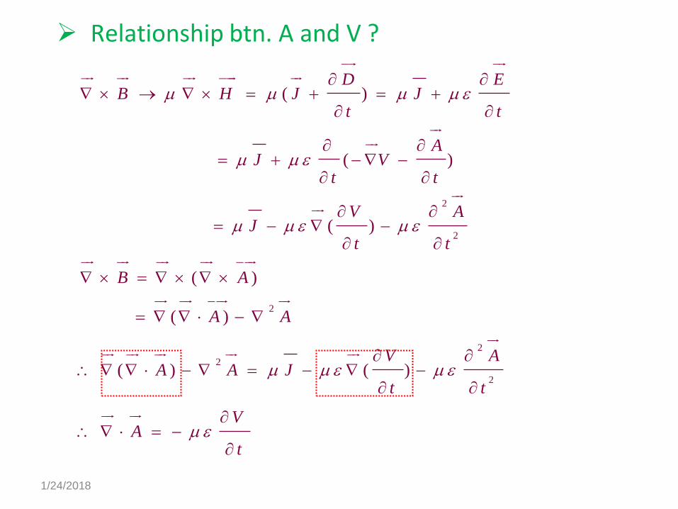
Relationship btn. A and V ?

2

2

2

2

2

2

( )

( )

( )

( )

( )

( ) ( )

D EB H J J

t t

AJ V

t t

V AJ

t t

B A

A A

V AA A J

t t

VA

t

1/24/2018

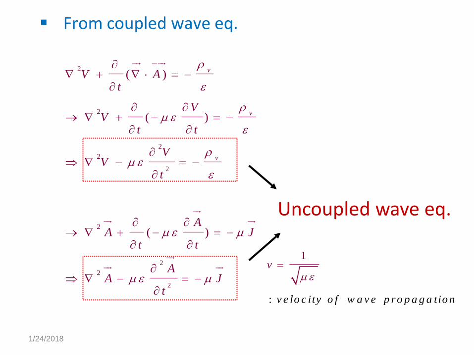
From coupled wave eq.

2

2

2

2

2

2

2

2

2

( )

( )

( )

v

v

v

V At

VV

t t

VV

t

AA J

t t

AA J

t

Uncoupled wave eq.

:

1

v e lo c ity o f w a v e p ro p a g a n

v

tio

1/24/2018

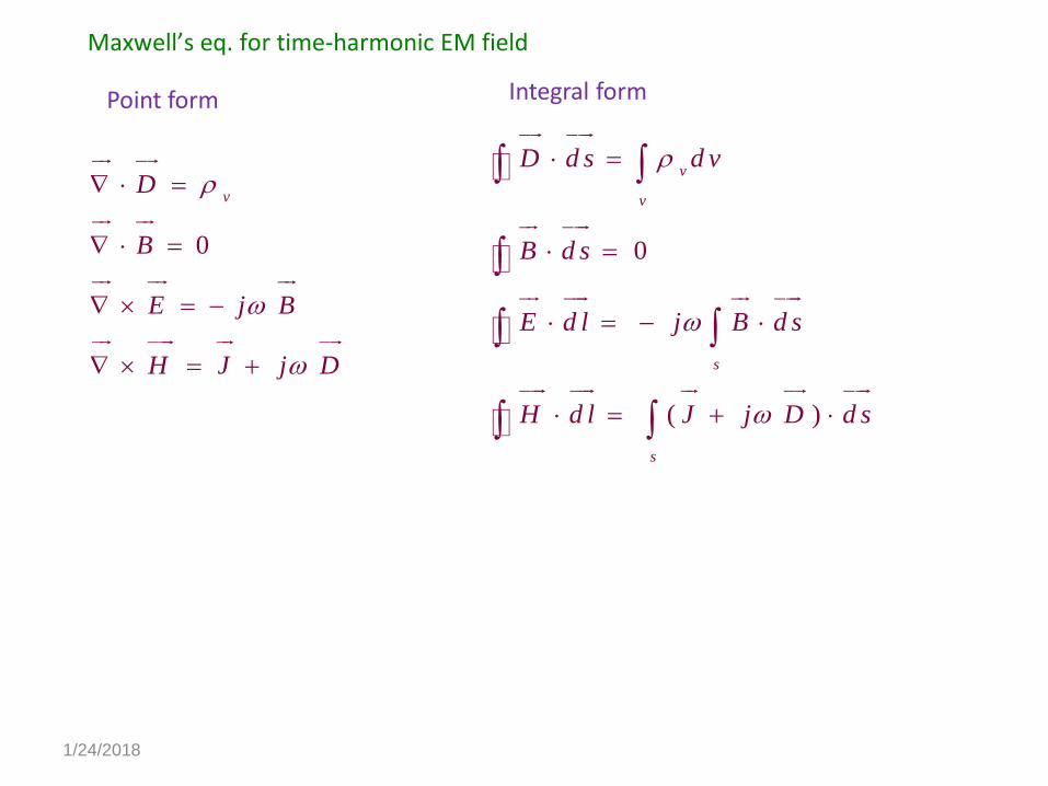
Maxwell’s eq. for time-harmonic EM field

0

vD

B

E j B

H J j D

0

( )

v

v

s

s

D d s d v

B d s

E d l j B d s

H d l J j D d s

Point form Integral form

1/24/2018

UNIT 3

UNIFORM PLANE WAVES

1/24/2018

Waves are means of transporting energy or informationfrom oneplace to another.

An EM wave are a means for transferring electromagnetic energy

Why Uniform plane waves?• defines a plane surface• the field strength is uniform everywhere A plane wave is a constant-frequency wave whose wave fronts

(surfaces of constant phase) are• infinite parallel planes• of constant amplitude normal to the phase velocity vector

Plane Waves in General

1/24/2018

1/24/2018

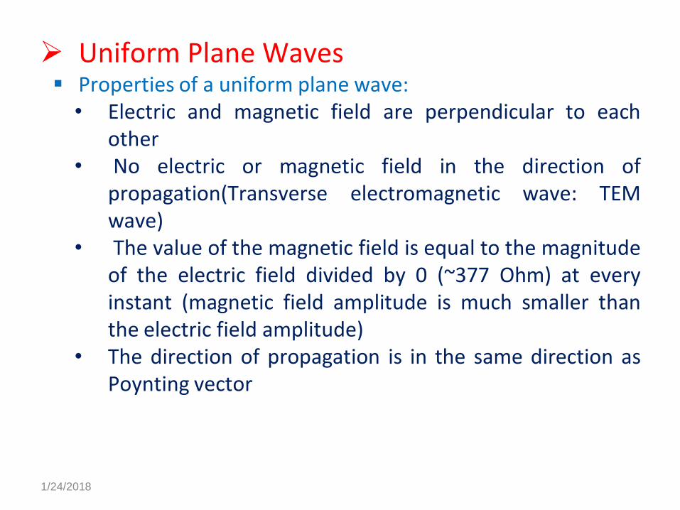
Uniform Plane Waves Properties of a uniform plane wave:

• Electric and magnetic field are perpendicular to eachother

• No electric or magnetic field in the direction ofpropagation(Transverse electromagnetic wave: TEMwave)

• The value of the magnetic field is equal to the magnitudeof the electric field divided by 0 (~377 Ohm) at everyinstant (magnetic field amplitude is much smaller thanthe electric field amplitude)

• The direction of propagation is in the same direction asPoynting vector

1/24/2018

Plane waves in various media

A media in electromagnetic is characterized by three parametersε,μ, and σ

Lossless medium: σ and μ are real, σ =0, so β is real Time-Domain Maxwell’s Equations in Differential Form for a Simple,

Source-Free, and Lossless Medium

0

0

HE E

t

EH H

t

1/24/2018

Wave Equations for Electromagnetic Waves in a Simple,Source-Free, Lossless Medium

The wave equations are not independent. Usually we solve the electric field wave equation and

determine H from E using Faraday’s law.

2

2

20

EE

t

2

2

20

HH

t

1/24/2018

Let us examine a possible plane wave solution given by

The wave equation for this field simplifies to

The general solution to this wave equation is

The functions p1(z-vpt) and p2 (z+vpt) represent uniformwaves propagating in the +z and -z directions respectively.

Once the electric field has been determined from the waveequation, the magnetic field must follow from Maxwell’sCurl equations.

2 2

2 20

x xE E

z t

ˆ ,x x

E a E z t

1 2,

x p pE z t p z v t p z v t

1/24/2018

The electric and magnetic fields are given by

The argument of the cosine function is the called theinstantaneous phase of the field:

The speed with which a constant value of instantaneousphase travels is called the phase velocity. For a losslessmedium, it is equal to and denoted by the same symbol asthe velocity of propagation

1 2

1 2

, c o s c o s

1, c o s c o s

x

y

E z t C t z C t z

H z t C t z C t z

,z t t z

1/24/2018

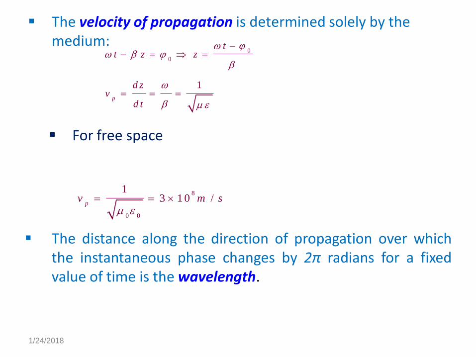
The velocity of propagation is determined solely by the medium:

The distance along the direction of propagation over whichthe instantaneous phase changes by 2π radians for a fixedvalue of time is the wavelength.

For free space

0

0

1

p

tt z z

d zv

d t

8

0 0

13 1 0 /

pv m s

1/24/2018

Lossy medium: Time-Domain Maxwell’s Equations in Differential Form for a

Simple, Source-Free, and Possibly Lossy Medium

0

0

E j H E

H j E H

m

j j

j j

1/24/2018

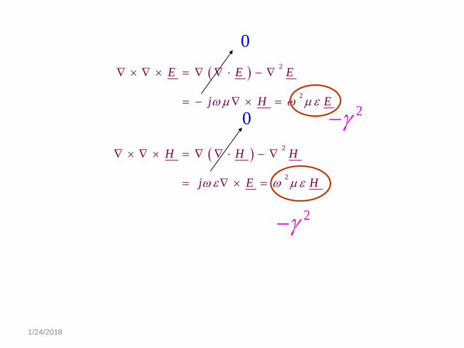
2

2

2

2

E E E

j H E

H H H

j E H

0

02

2

1/24/2018

Helmholtz Equations for Electromagnetic Waves

The Helmholtz equations are not independent. Usually we solve the electric field equation and determine

Hfrom E using Faraday’s law.

Assuming a plane wave solution of the form

The Helmholtz equation simplifies to

2 20E E

2 20H H

ˆx x

E a E z

2

2

20

x

x

d EE

d z

1/24/2018

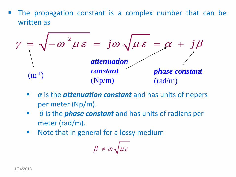
The propagation constant is a complex number that can bewritten as

attenuation

constant

(Np/m)

phase constant

(rad/m)(m-1)

α is the attenuation constant and has units of nepersper meter (Np/m).

β is the phase constant and has units of radians per meter (rad/m).

Note that in general for a lossy medium

2j j

1/24/2018

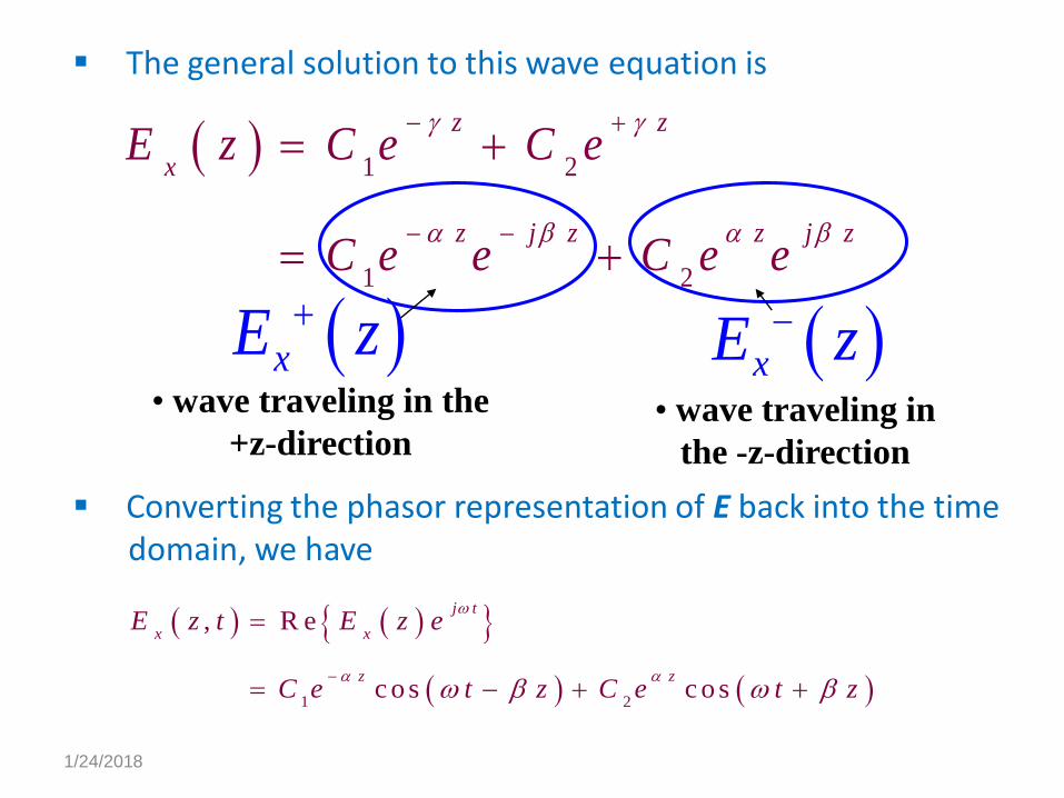
The general solution to this wave equation is

1 2

1 2

z z

x

z j z z j z

E z C e C e

C e e C e e

xE z xE z

• wave traveling in the

+z-direction• wave traveling in

the -z-direction

Converting the phasor representation of E back into the time domain, we have

1 2

, R e

c o s c o s

j t

x x

z z

E z t E z e

C e t z C e t z

1/24/2018

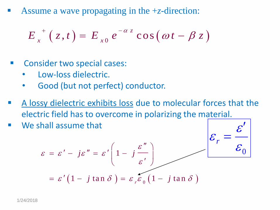
Assume a wave propagating in the +z-direction:

Consider two special cases:• Low-loss dielectric.• Good (but not perfect) conductor.

A lossy dielectric exhibits loss due to molecular forces that theelectric field has to overcome in polarizing the material.

We shall assume that

0

r

0, cos

z

x xE z t E e t z

0

1

1 ta n 1 ta nr

j j

j j

1/24/2018

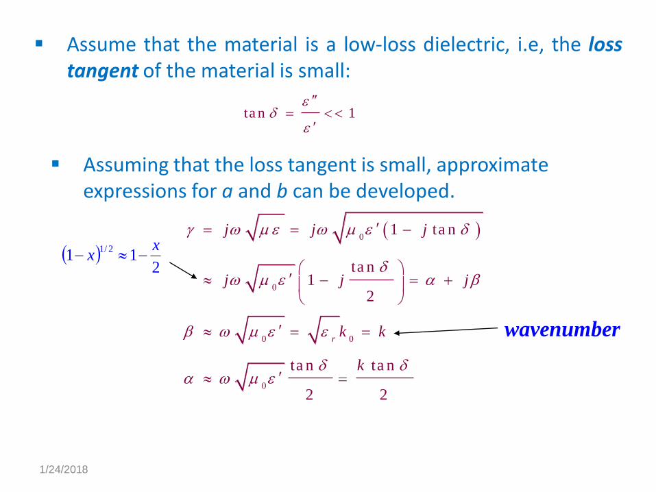
Assume that the material is a low-loss dielectric, i.e, the losstangent of the material is small:

Assuming that the loss tangent is small, approximate expressions for a and b can be developed.

2

112/1 x

x

wavenumber

ta n 1

0

0

0 0

0

1 ta n

ta n1

2

ta n ta n

2 2

r

j j j

j j j

k k

k

1/24/2018

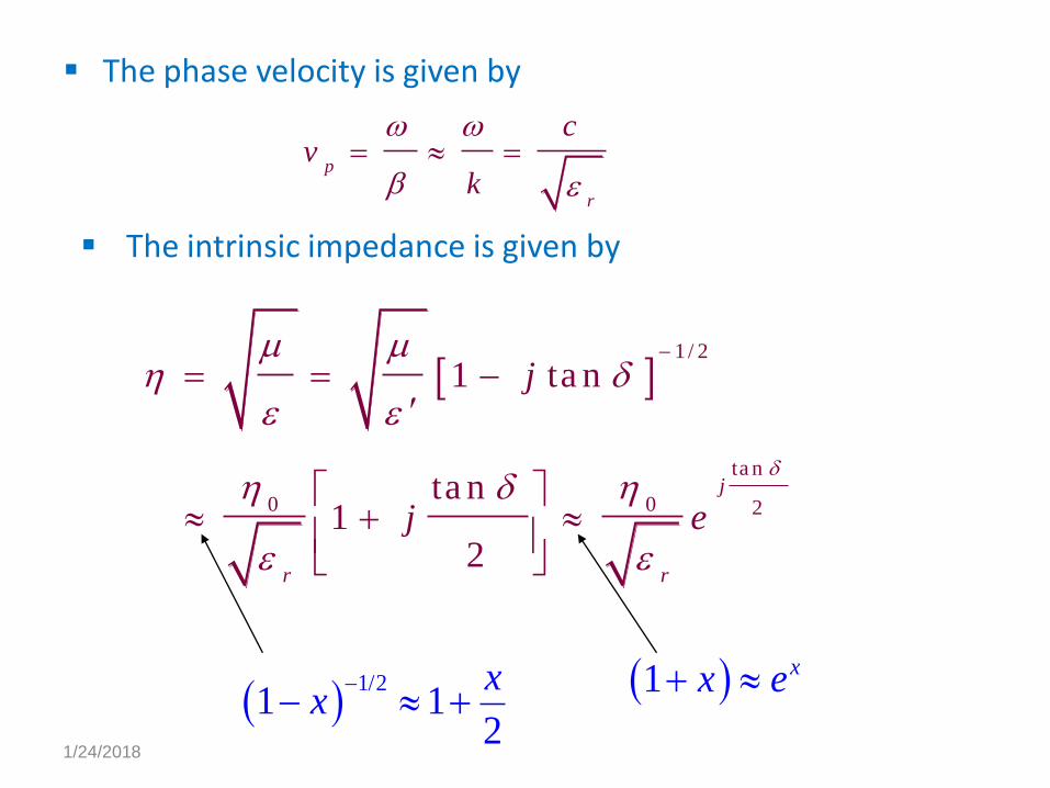
The phase velocity is given by

The intrinsic impedance is given by

1/2

1 12

xx

1 xx e

p

r

cv

k

1 / 2

ta n

0 0 2

1 ta n

ta n1

2

j

r r

j

j e

1/24/2018

In a perfect conductor, the electromagnetic field must vanish. In a good conductor, the electromagnetic field experiences

significant attenuation as it propagates. The properties of a good conductor are determined primarily

by its conductivity. For a good conductor

1

j

12

j j j j

j

2

2

1/24/2018

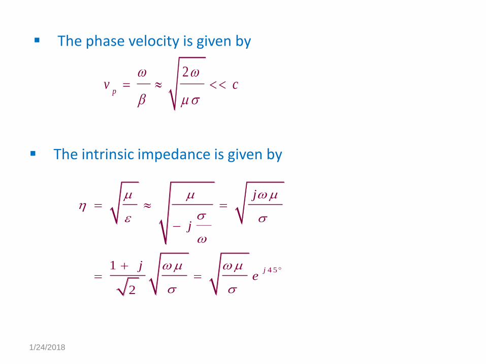
The phase velocity is given by

2

pv c

The intrinsic impedance is given by

4 51

2

j

j

j

je

1/24/2018

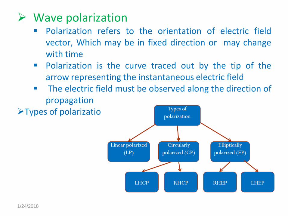
Wave polarization Polarization refers to the orientation of electric field

vector, Which may be in fixed direction or may changewith time

Polarization is the curve traced out by the tip of thearrow representing the instantaneous electric field

The electric field must be observed along the direction ofpropagation

Types of polarization

1/24/2018

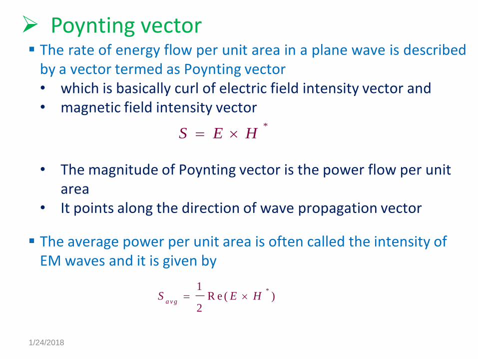
The rate of energy flow per unit area in a plane wave is describedby a vector termed as Poynting vector• which is basically curl of electric field intensity vector and• magnetic field intensity vector

• The magnitude of Poynting vector is the power flow per unit area

• It points along the direction of wave propagation vector

The average power per unit area is often called the intensity of EM waves and it is given by

Poynting vector

*S E H

*1R e ( )

2a v g

S E H

1/24/2018

UNIT 4 TRANSMISSION LINES CHARACTERISTICS

1/24/2018

TRANSMISSION LINES

Any physical structure that will guide an electromagnetic waveplace to place is called a Transmission Line.

Types of Transmission Lines

• Two wire line• Coaxial cable• Waveguide

o Rectangularo Circular

• Planar Transmission Lines

o Strip lineo Micro strip lineo Slot lineo Fin lineo Coplanar Waveguideo Coplanar slot line

1/24/2018

At low frequencies, the circuit elements areLumped voltage and current waves affect the entire circuit atthe same time.

At microwave frequenciesVoltage and current waves donot affect the entire circuit at the same time.

The circuit must be broken down into unit sections within

within which the circuit elements are considered to be lumped.

Low and High Frequency Transmission lines

1/24/2018

TRANSMISSION LINE PARAMETERS It is convenient to describe a transmission line in terms of its

line parameters, which are

• Resistance per unit length R,

• Inductance per unit length L,

• Conductance per unit length G,

• Capacitance per unit length C.

The line parameters R, L, G, and C are not discrete or lumped but distributed as shown in Figure.

For Each Line

LC = με and

1/24/2018

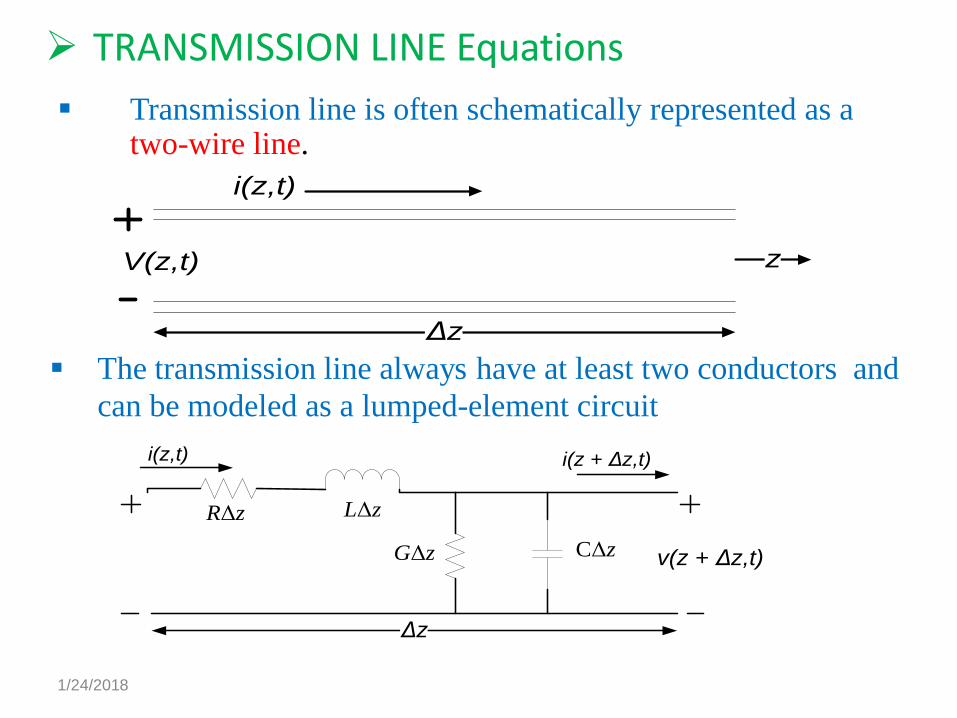
TRANSMISSION LINE Equations

Transmission line is often schematically represented as a two-wire line.

i(z,t)

V(z,t)

Δz

z

The transmission line always have at least two conductors and

can be modeled as a lumped-element circuit

RΔz LΔz

GΔz CΔz

i(z,t) i(z + Δz,t)

Δz

v(z + Δz,t)

1/24/2018

By using the Kirchoff’s voltage law, the wave equation for V(z) and I(z) can be written as:

2

2

20

d V zV z

d z

2

2

20

d I zI z

d z

j R j L G j C

γ is the complex propagation constant, which is function of

frequency.

α is the attenuation constant in nepers per unit length, β is the

phase constant in radians per unit length.

The traveling wave solution to the equation can be found as:

0 0

0 0

z z

z z

V z V e V e

I z I e I e

1/24/2018

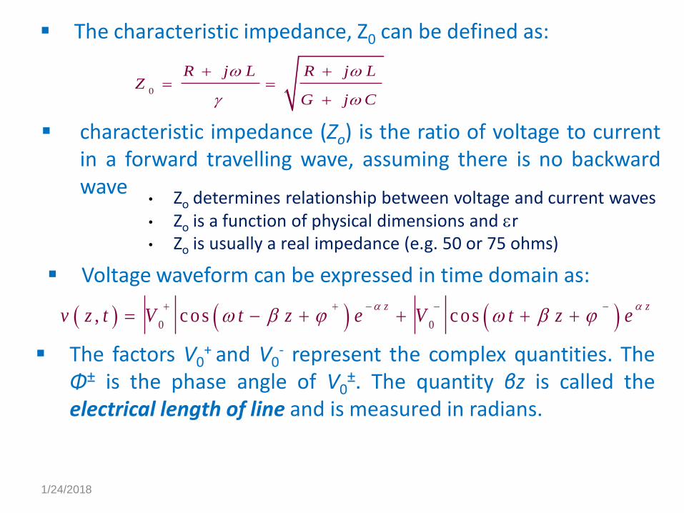
The characteristic impedance, Z0 can be defined as:

0

R j L R j LZ

G j C

characteristic impedance (Zo) is the ratio of voltage to currentin a forward travelling wave, assuming there is no backwardwave

• Zo determines relationship between voltage and current waves• Zo is a function of physical dimensions and r• Zo is usually a real impedance (e.g. 50 or 75 ohms)

Voltage waveform can be expressed in time domain as:

0 0, c os c os

z zv z t V t z e V t z e

The factors V0+ and V0

- represent the complex quantities. TheΦ± is the phase angle of V0

±. The quantity βz is called theelectrical length of line and is measured in radians.

1/24/2018

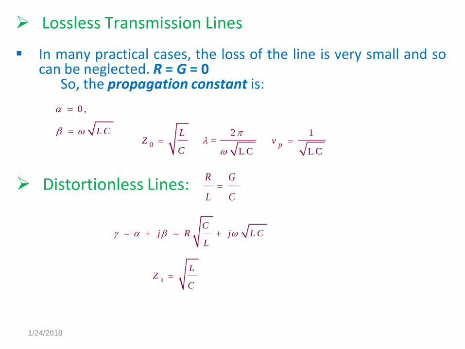
Lossless Transmission Lines

In many practical cases, the loss of the line is very small and socan be neglected. R = G = 0

So, the propagation constant is:

0 ,

L C

0

2 1 =

L C L Cp

LZ v

C

Distortionless Lines:R G

L C

Cj R j L C

L

0

LZ

C

1/24/2018

Low-Loss Transmission Lines

(1 ) (1 )

(1 ) (1 ) ( )2 2 2 2

R Gj j L j C

j L j C

R G R C G Lj L C j L C

j L j C L C

0

[1 ( ) ] 1[1 ( ) ]

[1 ] 2

R j L j L R j L L R G LZ j

G j C j C G j C C L C C

0

02 2

c d

R G Z

Z

L C

Lossy line has a linear phase factor as a function of frequency

1/24/2018

UNIT-VUHF TRANSMISSION LINES AND APPLICATIONS

1/24/2018

The Terminated Lossless TL j

0

0

0

0

is in c id e n

( )

t

[ ]

( )

v

[ ]

w a e

j z z

j z j z

j z

V z V e e

VI z e e

Z

V e

0 0

0 0

m a x

m in

2 0 lo g d B

1 W R

1

L

L

V Z Z

V Z Z

R L

VS

V

20

0

2

0

0 02

0

( ) ( 0 )

1 ta n

1 ta n

j l

j l

j l

j l

L

in j l

L

V el e

V e

e Z jZ lZ Z Z

e Z jZ l

Transmission line impedance equation

Reflection coefficient 0 1

Return loss (RL,dB) 0

Standing wave ratio 1

Match Mismatch(Total Reflection)

Match conditions

Zin

1/24/2018

Terminated in short circuit Terminated in open circuit

ljZZin

tan0

ljZZin

cot0

2

|in L l

Z Z

1/24/2018

2

1

in

L

ZZ

Z

Quarter-Wave Transformer A useful and practical circuit for impedance matching.

Defined as TL with length equals to ℓ=/4(+ n/2).

Perfect matching occurs at one frequency (odd multiple) but mismatch will occur at other frequencies.

Impedance matching is limited to real load impedances (complex load impedance can be transferred to real one, by transformation through an appropriate length of line.)

ℓ=(2/)(/4)= /

1 0 LZ Z R

In order for =0, one must have Zin = Z0, then

Insertion Loss (IL) ; (d B )2 0 lo g

T 1

IL T

1/24/2018

Generator and Load Mismatch

0

0

0

0

1 W R

1

l

l

l

g

g

g

l

l

Z Z

Z Z

Z Z

Z Z

S

Load matched to line Generator matched to line

Conjugate matching

Zl=Z0 ; l=0; Zin=Z0 ; SWR=1 Zin=Zg ; l 0 ; SWR>1

22

0

02

)(2

1

gg

gXRZ

ZVP

2

2

1

2 4 ( )

g

g

g g

RP V

R X

Zin=Zg* ; g 0 ; l 0 ; 0 ; SWR>1

21 1

2 4g

g

P VR

0in g

in g

Z Z

Z Z

Multiple reflections may add inphase to deliver more power P tothe load.

1/24/2018

The Smith Chart

The Smith chart is a plot of

21 1Γ Γ ; ( )

1 1

w h e re , 0 1 8 0

j j lZe e Z

Z

Z r jx

constant-r circles

constant-x circles

2 2 2

1w h e re c irc u le s c e n te r is

1( ) Γ ( ) ;

a t ( ,0 ) , r a d iu s is 1 1

1 1

r i

r

r

r r

r r

2 2 2;

w h e re c ir c u le s c e n te r is a t1 1

(1, , r a d iu s

1 1( 1) ( ) (

s)

)

i

r i

x

x x

x

F or p a ss ive im p e d a n c e 0 ; r x

1/24/2018