Electromagnetic Fields and Energy - ocw.mit.edu · Electromagnetic Fields and Energy. ......
49
MIT OpenCourseWare http://ocw.mit.edu Haus, Hermann A., and James R. Melcher. Electromagnetic Fields and Energy. Englewood Cliffs, NJ: Prentice-Hall, 1989. ISBN: 9780132490207. Please use the following citation format: Haus, Hermann A., and James R. Melcher, Electromagnetic Fields and Energy. (Massachusetts Institute of Technology: MIT OpenCourseWare). http://ocw.mit.edu (accessed [Date]). License: Creative Commons Attribution-NonCommercial-Share Alike. Also available from Prentice-Hall: Englewood Cliffs, NJ, 1989. ISBN: 9780132490207. Note: Please use the actual date you accessed this material in your citation. For more information about citing these materials or our Terms of Use, visit: http://ocw.mit.edu/terms
Transcript of Electromagnetic Fields and Energy - ocw.mit.edu · Electromagnetic Fields and Energy. ......

MIT OpenCourseWare httpocwmitedu
Haus Hermann A and James R Melcher Electromagnetic Fields and Energy Englewood Cliffs NJ Prentice-Hall 1989 ISBN 9780132490207
Please use the following citation format
Haus Hermann A and James R Melcher Electromagnetic Fields and Energy (Massachusetts Institute of Technology MIT OpenCourseWare) httpocwmitedu (accessed [Date]) License Creative Commons Attribution-NonCommercial-Share Alike
Also available from Prentice-Hall Englewood Cliffs NJ 1989 ISBN 9780132490207
Note Please use the actual date you accessed this material in your citation
For more information about citing these materials or our Terms of Use visit httpocwmiteduterms
13
ELECTRODYNAMIC FIELDS THE BOUNDARY VALUE POINT OF VIEW
130 INTRODUCTION
In the treatment of EQS and MQS systems we started in Chaps 4 and 8 reshyspectively by analyzing the fields produced by specified (known) sources Then we recognized that in the presence of materials at least some of these sources were induced by the fields themselves Induced surface charge and surface current denshysities were determined by making the fields satisfy boundary conditions In the volume of a given region fields were composed of particular solutions to the govshyerning quasistatic equations (the scalar and vector Poisson equations for EQS and MQS systems respectively) and those solutions to the homogeneous equations (the scalar and vector Laplace equation respectively) that made the total fields satisfy appropriate boundary conditions
We now embark on a similar approach in the analysis of electrodynamic fields Chapter 12 presented a study of the fields produced by specified sources (dipoles line sources and surface sources) and obeying the inhomogeneous wave equation Just as in the case of EQS and MQS systems in Chap 5 and the last half of Chap 8 we shall now concentrate on solutions to the homogeneous sourceshyfree equations These solutions then serve to obtain the fields produced by sources lying outside (maybe on the boundary) of the region within which the fields are to be found In the region of interest the fields generally satisfy the inhomogeneous wave equation However in this chapter where there are no sources in the volume of interest they satisfy the homogeneous wave equation It should come as no surprise that following this systematic approach we shall reencounter some of the previously obtained solutions
In this chapter fields will be determined in some limited region such as the volume V of Fig 1301 The boundaries might be in part perfectly conducting in the sense that on their surfaces E is perpendicular and the timeshyvarying H is tangential The surface current and charge densities implied by these conditions
1
2 Electrodynamic Fields The Boundary Value Point of View Chapter 13
Fig 1301 Fields in a limited region are in part due to sources induced on boundaries by the fields themselves
are not known until after the fields have been found If there is material within the region of interest it is perfectly insulating and of pieceshywise uniform permittivity and permeability micro 1 Sources J and ρ are specified throughout the volume and apshypear as driving terms in the inhomogeneous wave equations (1268) and (12632) Thus the H and E fields obey the inhomogeneous waveshyequations
part2H 2Hminus micro partt2
= minus times J (1)
2Eminus micropart2E
= ρ + micro
partJ (2)
partt2 partt
As in earlier chapters we might think of the solution to these equations as the sum of a part satisfying the inhomogeneous equations throughout V (particshyular solution) and a part satisfying the homogeneous wave equation throughout that region In principle the particular solution could be obtained using the sushyperposition integral approach taken in Chap 12 For example if an electric dipole were introduced into a region containing a uniform medium the particular solution would be that given in Sec 122 for an electric dipole The boundary conditions are generally not met by these fields They are then satisfied by adding an appropriate solution of the homogeneous wave equation2
In this chapter the source terms on the right in (1) and (2) will be set equal to zero and so we shall be concentrating on solutions to the homogeneous wave equation By combining the solutions of the homogeneous wave equation that satisfy boundary conditions with the sourceshydriven fields of the preceding chapter one can describe situations with given sources and given boundaries
In this chapter we shall consider the propagation of waves in some axial direction along a structure that is uniform in that direction Such waves are used to transport energy along pairs of conductors (transmission lines) and through
1 If the region is one of free space o and micro microorarr rarr2 As pointed out in Sec 127 this is essentially what is being done in satisfying boundary
conditions by the method of images
Sec 131 TEM Waves 3
waveguides (metal tubes at microwave frequencies and dielectric fibers at optical frequencies) We confine ourselves to the sinusoidal steady state
Sections 131shy133 study twoshydimensional modes between plane parallel conshyductors This example introduces the mode expansion of electrodynamic fields that is analogous to the expansion of the EQS field of the capacitive attenuator (in Sec 55) in terms of the solutions to Laplacersquos equation The principal and higher order modes form a complete set for the representation of arbitrary boundary conditions The example is a model for a strip transmission line and hence serves as an introshyduction to the subject of Chap 14 The highershyorder modes manifest properties much like those found in Sec 134 for hollow pipe guides
The dielectric waveguides considered in Sec 135 explain the guiding propshyerties of optical fibers that are of great practical interest Waves are guided by a dielectric core having permittivity larger than that of the surrounding medium but possess fields extending outside this core Such electromagnetic waves are guided because the dielectric core slows the effective velocity of the wave in the guide to the point where it can match the velocity of a wave in the surrounding region that propagates along the guide but decays in a direction perpendicular to the guide
The fields considered in Secs 131ndash133 offer the opportunity to reinforce the notions of quasistatics Connections between the EQS and MQS fields studied in Chaps 5 and 8 respectively and their corresponding electrodynamic fields are made throughout Secs 131ndash134
131 INTRODUCTION TO TEM WAVES
The E and H fields of transverse electromagnetic waves are directed transverse to the direction of propagation It will be shown in Sec 142 that such TEM waves propagate along structures composed of pairs of perfect conductors of arbitrary crossshysection The parallel plates shown in Fig 1311 are a special case of such a pair of conductors The direction of propagation is along the y axis With a source driving the conductors at the left the conductors can be used to deliver electrical energy to a load connected between the right edges of the plates They then function as a parallel plate transmission line
We assume that the plates are wide in the z direction compared to the spacing a and that conditions imposed in the planes y = 0 and y = minusb are independent of z so that the fields are also z independent In this section discussion is limited to either ldquoopenrdquo electrodes at y = 0 or ldquoshortedrdquo electrodes Techniques for dealing with arbitrarily terminated transmission lines will be introduced in Chap 14 The ldquoopenrdquo or ldquoshortedrdquo terminals result in standing waves that serve to illustrate the relationship between simple electrodynamic fields and the EQS and MQS limits These fields will be generalized in the next two sections where we find that the TEM wave is but one of an infinite number of modes of propagation along the y axis between the plates
If the plates are open circuited at the right as shown in Fig 1311 a voltage is applied at the left at y = minusb and the fields are EQS the E that results is x directed (The plates form a parallel plate capacitor) If they are ldquoshortedrdquo at the right and the fields are MQS the H that results from applying a current source at the left is z directed (The plates form a oneshyturn inductor) We are now looking
4 Electrodynamic Fields The Boundary Value Point of View Chapter 13
Fig 1311 Plane parallel plate transmission line
for solutions to Maxwellrsquos equations (1207)ndash(12010) that are similarly transverse to the y axis
E = Exix H = Hziz (1)
Fields of this form automatically satisfy the boundary conditions of zero tanshygential E and normal H (normal B) on the surfaces of the perfect conductors These fields have no divergence so the divergence laws for E and H [(1207) and (12010)] are automatically satisfied Thus the remaining laws Amperersquos law (1208) and Faradayrsquos law (1209) fully describe these TEM fields We pick out the only comshyponents of these laws that are not automatically satisfied by observing that partExpartt drives the x component of Amperersquos law and partHzpartt is the source term of the z component of Faradayrsquos law
partHz partEx = party partt (2)
partEx partHz = microparty partt (3)
The other components of these laws are automatically satisfied if it is assumed that the fields are independent of the transverse coordinates and thus depend only on y
The effect of the plates is to terminate the field lines so that there are no fields in the regions outside With Gaussrsquo continuity condition applied to the respective plates Ex terminates on surface charge densities of opposite sign on the respective electrodes
σs(x = 0) = Ex σs(x = a) = minusEx (4)
These relationships are illustrated in Fig 1312a The magnetic field is terminated on the plates by surface current densities
With Amperersquos continuity condition applied to each of the plates
Ky(x = 0) = minusHz Ky(x = a) = Hz (5)
5 Sec 131 TEM Waves
Fig 1312 (a) Surface charge densities terminating E of TEM field between electrodes of Fig 1311 (b) Surface current densities terminating H
these relationships are represented in Fig 1312b We shall be interested primarily in the sinusoidal steady state Between the
plates the fields are governed by differential equations having constant coefficients We therefore assume that the field response takes the form
Hz = Re H z(y)ejωt Ex = Re E
x(y)ejωt (6)
where ω can be regarded as determined by the source that drives the system at one of the boundaries Substitution of these solutions into (2) and (3) results in a pair of ordinary constant coefficient differential equations describing the y dependence of Ex and Hz Without bothering to write these equations out we know that they too will be satisfied by exponential functions of y Thus we proceed to look for solutions where the functions of y in (6) take the form exp(minusjkyy)
Hz = Re h ze
j(ωtminuskyy) Ex = Re ˆ exej(ωtminuskyy) (7)
Once again we have assumed a solution taking a product form Substitution into (2) then shows that
ex = ky
hz (8)minus ω
and substitution of this expression into (3) gives the dispersion equation
ky = plusmnβ β equiv ωradic
micro = ω
(9) c
For a given frequency there are two values of ky A linear combination of the solutions in the form of (7) is therefore
Hz = Re [A+ eminusjβy + Aminusejβy ]ejωt (10)
The associated electric field follows from (8) evaluated for the plusmn waves respectively using ky = plusmnβ
eminusjβy jβy]ejωt Ex = minusRe
micro[A+ minus Aminuse (11)
The amplitudes of the waves A+ and Aminus are determined by the boundary conditions imposed in planes perpendicular to the y axis The following example
6 Electrodynamic Fields The Boundary Value Point of View Chapter 13
Fig 1313 (a) Shorted transmission line driven by a distributed curshyrent source (b) Standing wave fields with E and H shown at times differing by 90 degrees (c) MQS fields in limit where wavelength is long compared to length of system
illustrates how the imposition of these longitudinal boundary conditions determines the fields It also is the first of several opportunities we now use to place the EQS and MQS approximations in perspective
Example 1311 Standing Waves on a Shorted Parallel Plate Transmission Line
In Fig 1313a the parallel plates are terminated at y = 0 by a perfectly conducting plate They are driven at y = minusb by a current source Id distributed over the width w Thus there is a surface current density Ky = Idw equiv Ko imposed on the lower plate at y = minusb Further in this example we will assume that a distribution of sources is used in the plane y = minusb to make this driving surface current density uniform over that plane In summary the longitudinal boundary conditions are
Ex(0 t) = 0 (12)
Hz(minusb t) = minusRe K oe
jωt (13)
To make Ex as given by (11) satisfy the first of these boundary conditions we must have the amplitudes of the two traveling waves equal
A+ = Aminus (14)
With this relation used to eliminate A+ in (10) it follows from (13) that
A+ K o
= (15)minus 2 cos βb
We have found that the fields between the plates take the form of standing waves
minusRe ˆ cos βy jωt Hz = Ko e (16) cos βb
Cite as Markus Zahn course materials for 6641 Electromagnetic Fields Forces and Motion Spring 2005 MIT OpenCourseWare (httpocwmitedu) Massachusetts Institute of Technology Downloaded on [DD Month YYYY]
7 Sec 131 TEM Waves
Ex = minusRe jK o
micro
sin βy ejωt (17)
cos βb
Note that E and H are 90 out of temporal phase3 When one is at its peak the other is zero The distributions of E and H shown in Fig 1313b are therefore at different instants in time
Every halfshywavelength πβ from the short E is again zero as sketched in Fig 1313b Beginning at a distance of a quartershywavelength from the short the magnetic field also exhibits nulls at halfshywavelength intervals Adjacent peaks in a given field are 180 degrees out of temporal phase
The MQS Limit If the driving frequency is so low that a wavelength is much longer than the length b we have
2πb = βb 1 (18)
λ
In this limit the fields are those of a oneshyturn inductor That is with sin(βy) asymp βy and cos(βy) asymp 1 (16) and (17) become
Hz rarr minusRe K oe
jωt (19)
Ex rarr minusRe K ojωmicroyejωt (20)
The magnetic field intensity is uniform throughout and the surface current density circulates uniformly around the oneshyturn loop The electric field increases in a linear fashion from zero at the short to a maximum at the source where the source voltage is
a jωt dλ
v(t) = Ex(minusb t)dx = Re K ojωmicrobae = (21)
dt0
To make it clear that these are the fields of a oneshyturn solenoid (Example 844) the flux linkage λ has been identified as
λ = L di
dt i = Re Kowejωt L =
abmicro
w (22)
where L is the inductance
The MQS Approximation In Chap 8 we would have been led to these same limiting fields by assuming at the outset that the displacement current the term on the right in (2) is negligible Then this oneshydimensional form of Amperersquos law and (1) requires that
partHz times H asymp 0 rArr party
asymp 0 rArr Hz = Hz(t) = minusRe K oe
jωt (23)
If we now use this finding in Faradayrsquos law (3) integration on y and use of the boundary condition of (12) gives the same result for E as found taking the lowshyfrequency limit (20)
3 In making this and the following deductions it is helpful to take K o as being real
8 Electrodynamic Fields The Boundary Value Point of View Chapter 13
Fig 1314 (a) Open circuit transmission line driven by voltage source (b) E and H at times that differ by 90 degrees (c) EQS fields in limit where wavelength is long compared to b
In the previous example the longitudinal boundary conditions (conditions imposed at planes of constant y) could be satisfied exactly using the TEM mode alone The short at the right and the distributed current source at the left each imposed a condition that was like the TEM fields independent of the transverse coordinates In almost all practical situations longitudinal boundary conditions which are independent of the transverse coordinates (used to describe transmission lines) are approximate The open circuit termination at y = 0 shown in Fig 1314 is a case in point as is the source which in this case is not distributed in the x direction
If a longitudinal boundary condition is independent of z the fields are in principle still two dimensional Between the plates we can therefore think of satshyisfying the longitudinal boundary conditions using a superposition of the modes to be developed in the next section These consist of not only the TEM mode conshysidered here but of modes having an x dependence A detailed evaluation of the coefficients specifying the amplitudes of the highershyorder modes brought in by the transverse dependence of a longitudinal boundary condition is illustrated in Sec 133 There we shall find that at low frequencies where these highershyorder modes are governed by Laplacersquos equation they contribute to the fields only in the vicinity of the longitudinal boundaries As the frequency is raised beyond their respective cutoff frequencies the highershyorder modes begin to propagate along the y axis and so have an influence far from the longitudinal boundaries
Here where we wish to restrict ourselves to situations that are well described by the TEM modes we restrict the frequency range of interest to well below the lowest cutoff frequency of the lowest of the highershyorder modes
Given this condition ldquoend effectsrdquo are restricted to the neighborhood of a longitudinal boundary Approximate boundary conditions then determine the disshytribution of the TEM fields which dominate over most of the length In the open
9 Sec 131 TEM Waves
Fig 1315 The surface current density and hence Hz go to zero in the vicinity of the open end
circuit example of Fig 1314a application of the integral charge conservation law to a volume enclosing the end of one of the plates as illustrated in Fig 1315 shows that Ky must be essentially zero at y = 0 For the TEM fields this implies the boundary condition4
Hz(0 t) = 0 (24)
At the left end the vertical segments of perfect conductor joining the voltage source to the parallel plates require that Ex be zero over these segments We shall show later that the highershyorder modes do not contribute to the line integral of E between the plates Thus in so far as the TEM fields are concerned the requirement is that a Vd
Vd(t) = Ex(minusb t)dx Ex(minusb t) = (25) 0
rArr a
Example 1312 Standing Waves on an OpenshyCircuit Parallel Plate Transmission Line
Consider the parallel plates ldquoopenrdquo at y = 0 and driven by a voltage source at y = minusb Boundary conditions are then
Hz(0 t) = 0 Ex(minusb t) = Re Vd ejωta (26)
Evaluation of the coefficients in (10) and (11) so that the boundary conditions in (26) are satisfied gives
VdA+ = minusAminus = minus
2a cos βb
micro (27)
It follows that the TEM fields between the plates (10) and (11) are
Vd sin βy jωt Hz = Re j
micro e (28) a cos βb
Vd cos βy jωt Ex = Re e (29) a cos βb
These distributions of H and E are shown in Fig 1314 at times that differ by 90 degrees The standing wave is similar to that described in the previous example except that it is now E rather than H that peaks at the open end
4 In the region outside the fields are not confined by the plates As a result there is actually some radiation from the open end of the line and this too is not represented by (24) This effect is small if the plate spacing is small compared to a wavelength
10 Electrodynamic Fields The Boundary Value Point of View Chapter 13
The EQS Limit In the low frequency limit where the wavelength is much longer than the length of the plates so that βb 1 the fields given by (28) and (29) become
Vd jωt Hz Re j ωye (30)rarr a
Vd jωt Ex Re e (31)rarr a
At low frequencies the fields are those of a capacitor The electric field is uniform and simply equal to the applied voltage divided by the spacing The magnetic field varies in a linear fashion from zero at the open end to its peak value at the voltage source Evaluation of minusHz at z = minusb gives the surface current density and hence the current i provided by the voltage source
i = Re jω bw
Vdejωt (32) a
Note that this expression implies that
dq bw i = q = CVd C = (33)
dt a
so that the limiting behavior is indeed that of a plane parallel capacitor
EQS Approximation How would the quasistatic fields be predicted in terms of the TEM fields If quasistatic we expect the system to be EQS Thus the magnetic induction is negligible so that the rightshyhand side of (3) is approximated as being equal to zero
partEx times E asymp 0 rArr party
asymp 0 (34)
It follows from integration of this expression and using the boundary condition of (26b) that the quasistatic E is
VdEx = (35)
a
In turn this result provides the displacement current density in Amperersquos law the rightshyhand side of (2)
partHz d Vd
(36)party
dt a
The rightshyhand side of this expression is independent of y Thus integration with respect to y with the ldquoconstantrdquo of integration evaluated using the boundary condition of (26a) gives
d yHz Vd (37)
dt a
For the sinusoidal voltage drive assumed at the outset in the description of the TEM waves this expression is consistent with that found in taking the quasistatic limit (30)
Sec 132 Parallel Plate Modes 11
Demonstration 1311 Visualization of Standing Waves
A demonstration of the fields described by the two previous examples is shown in Fig 1316 A pair of sheet metal electrodes are driven at the left by an oscillator A fluorescent lamp placed between the electrodes is used to show the distribution of the rms electric field intensity
The gas in the tube is ionized by the oscillating electric field Through the fieldshyinduced acceleration of electrons in this gas a sufficient velocity is reached so that collisions result in ionization and an associated optical radiation What is seen is a time average response to an electric field that is oscillating far more rapidly than can be followed by the eye
Because the light is proportional to the magnitude of the electric field the observed 075 m distance between nulls is a halfshywavelength It can be inferred that the generator frequency is f = cλ = 3times 10815 = 200 MHz Thus the frequency is typical of the lower VHF television channels
With the right end of the line shorted the section of the lamp near that end gives evidence that the electric field there is indeed as would be expected from Fig 1313b where it is zero at the short Similarly with the right end open there is a peak in the light indicating that the electric field near that end is maximum This is consistent with the picture given in Fig 1314b In going from an open to a shorted condition the positions of peak light intensity and hence of peak electric field intensity are shifted by λ4
12 Electrodynamic Fields The Boundary Value Point of View Chapter 13
Fig 1321 (a) Plane parallel perfectly conducting plates (b) Coaxial geshyometry in which zshyindependent fields of (a) might be approximately obtained without edge effects
132 TWOshyDIMENSIONAL MODES BETWEEN PARALLEL PLATES
This section treats the boundary value approach to finding the fields between the perfectly conducting parallel plates shown in Fig 1321a Most of the mathematical ideas and physical insights that come from a study of modes on perfectly conducting structures that are uniform in one direction (for example parallel wire and coaxial transmission lines and waveguides in the form of hollow perfectly conducting tubes) are illustrated by this example In the previous section we have already seen that the plates can be used as a transmission line supporting TEM waves In this and the next section we shall see that they are capable of supporting other electromagnetic waves
Because the structure is uniform in the z direction it can be excited in such a way that fields are independent of z One way to make the structure approximately uniform in the z direction is illustrated in Fig 1321b where the region between the plates becomes the annulus of coaxial conductors having very nearly the same radii Thus the difference of these radii becomes essentially the spacing a and the z coordinate maps into the φ coordinate Another way is to make the plates very wide (in the z direction) compared to their spacing a Then the fringing fields from the edges of the plates are negligible In either case the understanding is that the field excitation is uniformly distributed in the z direction The fields are now assumed to be independent of z
Because the fields are two dimensional the classifications and relations given in Sec 126 and summarized in Table 1283 serve as our starting point Cartesian coordinates are appropriate because the plates lie in coordinate planes Fields either have H transverse to the x minus y plane and E in the x minus y plane (TM) or have E transverse and H in the x minus y plane (TE) In these cases Hz and Ez are taken as the functions from which all other field components can be derived We consider sinusoidal steady state solutions so these fields take the form
jωt Hz = Re Hz(x y)e (1) jωt Ez = Re Ez(x y)e (2)
Sec 132 Parallel Plate Modes 13
These field components respectively satisfy the Helmholtz equation (1269) and (12633) in Table 1283 and the associated fields are given in terms of these components by the remaining relations in that table
Once again we find product solutions to the Helmholtz equation where Hz
and Ez are assumed to take the form X(x)Y (y) This formalism for reducing a partial differential equation to ordinary differential equations was illustrated for Helmholtzrsquos equation in Sec 126 This time we take a more mature approach based on the observation that the coefficients of the governing equation are indeshypendent of y (are constants) As a result Y (y) will turn out to be governed by a constant coefficient differential equation This equation will have exponential solushytions Thus with the understanding that ky is a yet to be determined constant (that will turn out to have two values) we assume that the solutions take the specific product forms
H z = h
z(x)eminusjkyy (3)
E z = ez(x)eminusjkyy (4)
Then the field relations of Table 1283 become
TM Fields d2hz 2ˆ+ p hz = 0 (5)dx2
where p2 equiv ω2micro minus k2 y
ky ˆex = minus ω
hz (6)
1 dhz ey = minus
jω dx (7)
TE Fields d2ez 2+ q ez = 0 (8)dx2
where q2 equiv ω2micro minus k2 y
h x =
ky ez (9)
ωmicro
1 dezh
y = jωmicro dx
(10)
The boundary value problem now takes a classic form familiar from Sec 55 What values of p and q will make the electric field tangential to the plates zero For the TM fields ey = 0 on the plates and it follows from (7) that it is the derivative of Hz that must be zero on the plates For the TE fields Ez must itself be zero at the plates Thus the boundary conditions are
TM Fields dh
z (0) = 0 dh
z (a) = 0 (11)dx dx
14 Electrodynamic Fields The Boundary Value Point of View Chapter 13
Fig 1322 Dependence of fundamental fields on x
TE Fields ez(0) = 0 ez(a) = 0 (12)
To check that all of the conditions are indeed met at the boundaries note that if (11) is satisfied there is neither a tangential E nor a normal H at the boundaries for the TM fields (There is no normal H whether the boundary condition is satisfied or not) For the TE field Ez is the only electric field and making Ez=0 on the boundaries indeed guarantees that Hx = 0 there as can be seen from (9)
Representing the TM modes the solution to (5) is a linear combination of sin(px) and cos(px) To satisfy the boundary condition (11) at x = 0 we must select cos(px) Then to satisfy the condition at x = a it follows that p = pn = nπa n = 0 1 2
ˆ (13)hz prop cos pnx
nπ pn = n = 0 1 2 (14)
a
These functions and the associated values of p are called eigenfunctions and eigenshyvalues respectively The solutions that have been found have the x dependence shown in Fig 1322a
From the definition of p given in (5) it follows that for a given frequency ω (presumably imposed by an excitation) the wave number ky associated with the nshyth mode is
ω2micro minus (nπa)2 ω2micro gt (nπa)2
ky equiv plusmnβn βn equiv minusj
(nπa)2 minus ω2micro ω2micro lt (nπa)2 (15)
Similar reasoning identifies the modes for the TE fields Of the two solutions to (8) the one that satisfies the boundary condition at x = 0 is sin(qx) The second boundary condition then requires that q take on certain eigenvalues qn
ez prop sin qnx (16)
nπ qn = (17)
a
Sec 132 Parallel Plate Modes 15
The x dependence of Ez is then as shown in Fig 1322b Note that the case n = 0 is excluded because it implies a solution of zero amplitude
For the TE fields it follows from (17) and the definition of q given with (8) that5
ω2micro minus (nπa)2 ω2micro gt (nπa)2 ky equiv plusmnβn βn equiv minusj
(nπa)2 minus ω2micro ω2micro lt (nπa)2
(18)
In general the fields between the plates are a linear combination of all of the modes In superimposing these modes we recognize that ky = plusmnβn Thus with coefficients that will be determined by boundary conditions in planes of constant y we have the solutions
TM Modes
eminusjβoy + Aminus jβoyHz =Re A+
o o e infin
eminusjβny + Aminus nπ jωt (19)
+
A+ n n e
jβny cos x
e
a n=1
TE Modes
infin
eminusjβny + Cminusenπ jωt Ez = Re
Cn
+ n
jβny sin x e (20)
a n=1
We shall refer to the nshyth mode represented by these fields as the TMn or TEn
mode respectively We now make an observation about the TM0 mode that is of farshyreaching
significance Its distribution of Hz has no dependence on x [(13) with pn = 0] As a result Ey = 0 according to (7) Thus for the TM0 mode both E and H are transverse to the axial direction y This special mode represented by the n = 0 terms in (19) is therefore the transverse electromagnetic (TEM) mode featured in the previous section One of its most significant features is that the relation between frequency ω and wave number in the y direction ky [(15) with n = 0] is ky = plusmnω
radicmicro = plusmnωc the same as for a uniform electromagnetic plane wave
Indeed as we saw in Sec 131 it is a uniform plane wave The frequency dependence of ky for the TEM mode and for the highershyorder
TMn modes given by (15) are represented graphically by the ω minus ky plot of Fig 1323 For a given frequency ω there are two values of ky which we have called plusmnβn The dashed curves represent imaginary values of ky Imaginary values correspond to exponentially decaying and ldquogrowingrdquo solutions An exponentially ldquogrowingrdquo solution is in fact a solution that decays in the minusy direction Note that the switch from exponentially decaying to propagating fields for the highershyorder modes occurs at the cutoff frequency
1 nπ ωcn = radic
micro a
(21)
5 For the particular geometry considered here it has turned out that the eigenvalues pn and qn are the same (with the exception of n = 0) This coincidence does not occur with boundaries having other geometries
16 Electrodynamic Fields The Boundary Value Point of View Chapter 13
Fig 1323 Dispersion relation for TM modes
Fig 1324 Dispersion relation for TE modes
The velocity of propagation of points of constant phase (for example a point at which a field component is zero) is ωky Figure 1323 emphasizes that for all but the TEM mode the phase velocity is a function of frequency The equation relating ω to ky represented by this figure (15) is often called the dispersion equation
The dispersion equation for the TE modes is shown in Fig 1324 Although the field distributions implied by each branch are very different in the case of the plane parallel electrodes considered here the curves are the same as those for the TMn=0 modes
The next section will provide greater insight into the highershyorder TM and TE modes
Sec 133 TE and TM Standing Waves 17
133 TE AND TM STANDING WAVES BETWEEN PARALLEL PLATES
In this section we delve into the relationship between the twoshydimensional highershyorder modes derived in Sec 132 and their sources The examples are chosen to relate directly to case studies treated in quasistatic terms in Chaps 5 and 8
The matching of a longitudinal boundary condition by a superposition of modes may at first seem to be a purely mathematical process However even qualishytatively it is helpful to think of the influence of an excitation in terms of the resulting modes For quasistatic systems this has already been our experience For the purshypose of estimating the dependence of the output signal on the spacing b between excitation and detection electrodes the EQS response of the capacitive attenuator of Sec 55 could be pictured in terms of the lowestshyorder mode In the electrodyshynamic situations of interest here it is even more common that one mode dominates Above its cutoff frequency a given mode can propagate through a waveguide to reshygions far removed from the excitation
Modes obey orthogonality relations that are mathematically useful for the evaluation of the mode amplitudes Formally the mode orthogonality is implied by the differential equations governing the transverse dependence of the fundamental field components and the associated boundary conditions For the TM modes these are (1325) and (13211)
TM Modes d2hzn + p 2nh
zn = 0 (1)dx2
where dh
zn (a) = 0 dhzn (0) = 0
dx dx
and for the TE modes these are (1328) and (13212)
TE Modes d2ezn + qn
2 ezn = 0 (2)dx2
where ezn(a) = 0 ezn(0) = 0
The word ldquoorthogonalrdquo is used here to mean that
a ˆ ˆhznhzmdx = 0 n = m (3)
0
a
eznezmdx = 0 n = m (4) 0
These properties of the modes can be seen simply by carrying out the integrals using the modes as given by (13213) and (13216) More fundamentally they can be deduced from the differential equations and boundary conditions themselves (1) and (2) This was illustrated in Sec 55 using arguments that are directly applicable here [(5520)ndash(5526)]
18 Electrodynamic Fields The Boundary Value Point of View Chapter 13
Fig 1331 Configuration for excitation of TM waves
The following two examples illustrate how TE and TM modes can be excited in waveguides In the quasistatic limit the configurations respectively become identical to EQS and MQS situations treated in Chaps 5 and 8
Example 1331 Excitation of TM Modes and the EQS Limit
In the configuration shown in Fig 1331 the parallel plates lying in the planes x = 0 and x = a are shorted at y = 0 by a perfectly conducting plate The excitation is provided by distributed voltage sources driving a perfectly conducting plate in the plane y = b These sources constrain the integral of E across narrow insulating gaps of length Δ between the respective edges of the upper plate and the adjacent plates All the conductors are modeled as perfect The distributed voltage sources maintain the twoshydimensional character of the fields even as the width in the z direction becomes long compared to a wavelength Note that the configuration is identical to that treated in Sec 55 Therefore we already know the field behavior in the quasistatic (low frequency) limit
In general the twoshydimensional fields are the sum of the TM and TE fields However here the boundary conditions can be met by the TM fields alone Thus we begin with Hz (13219) expressed as a single sum
(A+ eminusjβny jβny nπ jωt Hz = Re
infin
n + Aminusn e ) cos xe (5)
a n=0
This field and the associated E satisfy the boundary conditions on the parallel plates at x = 0 and x = a Boundary conditions are imposed on the tangential E at the longitudinal boundaries where y = 0
Ex(x 0 t) = 0 (6)
Sec 133 TE and TM Standing Waves 19
and at the driving electrode where y = b We assume here that the gap lengths Δ are small compared to other dimensions of interest Then the electric field within each gap is conservative and the line integral of Ex across the gaps is equal to the gap voltages plusmnv Over the region between x = Δ and x = a minus Δ the perfectly conducting electrode makes Ex = 0
a Δ Ex(x b t)dx = v Ex(x b t)dx = minusv (7)
aminusΔ 0
Because the longitudinal boundary conditions are on Ex we substitute Hz
as given by (5) into the x component of Faradayrsquos law [(1266) of Table 1283] to obtain
infin minusβn (A+ eminusjβny minus Aminuse
nπ jωt Ex = Re
n n jβny
cos x
e (8)
ω a n=0
To satisfy the condition at the short (6) A+ = nn Aminus and (8) becomes
2jβn A+ nπ jωt Ex = Re
infinn sin βny cos x
e (9)
ω a n=0
This set of solutions satisfies the boundary conditions on three of the four boundaries What we now do to satisfy the ldquolastrdquo boundary condition differs little from what was done in Sec 55 The A+rsquos are adjusted so that the summation ofn
product solutions in (9) matches the boundary condition at y = b summarized by (7) Thus we write (9) with y = b on the right and with the function representing (7) on the left This expression is multiplied by the mrsquoth eigenfunction cos(mπxa) and integrated from x = 0 to x = a
a a infin n
E
x(x b) cos mπx
dx = 2jβnA+
sin βnb a ω
middot 0 0 n=0 (10)
nπ mπ cos x cos xdx
a a
Because the intervals where E x(x b) is finite are so small the cosine function can
be approximated by a constant namely plusmn1 as appropriate On the rightshyhand side of (10) we exploit the orthogonality condition so as to pick out only one term in the infinite series
v[minus1 + cos mπ] =2jβm
sin βmb a
A+ (11)ω 2
m
Of the infinite number of terms in the integral on the right in (10) only the term where n = m has contributed The coefficients follow from solving (11) and replacing m nrarr
0 n evenA+ minus2ωv
n = n odd (12) jβna sin βnb
20 Electrodynamic Fields The Boundary Value Point of View Chapter 13
With the coefficients A+ = Aminus now determined we can evaluate all of the n n
fields Substitution into (5) and (8) and into the result using (1267) from Table 1283 gives infin
4jωv cos βny nπ
jωtHz = Re
cos x e (13)βna sin βnb a
n=1 odd
infin minus4ˆ v sin βny nπ
jωt Ex = Re
cos x e (14) a sin βnb a
n=1 odd
infin 4nπ v cos βny nπ
jωt Ey = Re
sin x e (15)
a (βna) sin βnb a n=1 odd
Note the following aspects of these fields (which we can expect to see in Demonshystration 1331) First the magnetic field is directed perpendicular to the xminusy plane Second by making the excitation symmetric we have eliminated the TEM mode As a result the only modes are of order n = 1 and higher Third at frequencies below the cutoff for the TM1 mode βy is imaginary and the fields decay in the y direction6 Indeed in the quasistatic limit where ω2micro (πa)2 the electric field is the same as that given by taking the gradient of (559) In this same quasistatic limit the magnetic field would be obtained by using this quasistatic E to evaluate the displacement current and then solving for the resulting magnetic field subject to the boundary condition that there be no normal flux density on the surfaces of the perfect conductors Fourth above the cutoff frequency for the n = 1 mode but below the cutoff for the n = 2 mode we should find standing waves having a wavelength 2πβ1
Finally note that each of the expressions for the field components has sin(βnb) in its denominator With the frequency adjusted such that βn = nπb this function goes to zero and the fields become infinite This resonance condition results in an infinite response because we have pictured all of the conductors as perfect It occurs when the frequency is adjusted so that a wave reflected from one boundary arrives at the other with just the right phase to reinforce upon a second reflection the wave currently being initiated by the drive
The following experiment gives the opportunity to probe the fields that have been found in the previous example In practical terms the structure considered might be a parallel plate waveguide
Demonstration 1331 Evanescent and Standing TM Waves
The experiment shown in Fig 1332 is designed so that the field distributions can be probed as the excitation is varied from below to above the cutoff frequency of the TM1 mode The excitation structures are designed to give fields approximating those found in Example 1331 For convenience a = 48 cm so that the excitation frequency ranges above and below a cutshyoff frequency of 31 GHz The generator is modulated at an audible frequency so that the amplitude of the detected signal is converted to ldquoloudnessrdquo of the tone from the loudspeaker
In this TM case the driving electrode is broken into segments each insulated from the parallel plates forming the waveguide and each attached at its center to a
6 sin(ju) = j sinh(u) and cos(ju) = cosh(u)
Sec 133 TE and TM Standing Waves 21
Fig 1332 Demonstration of TM evanescent and standing waves
coaxial line from the generator The segments insure that the fields applied to each part of the electrode are essentially in phase (The cables feeding each segment are of the same length so that signals arrive at each segment in phase) The width of the structure in the z direction is of the order of a wavelength or more to make the fields two dimensional (Remember in the vicinity of the lowest cutoff frequency a is about oneshyhalf wavelength) Thus if the feeder were attached to a contiguous electrode at one point there would be a tendency for standing waves to appear on the excitation electrode much as they did on the wire antennae in Sec 124 In the experiment the segments are about a quartershywavelength in the z direction but of course about a halfshywavelength in the x direction
In the experiment H is detected by means of a oneshyturn coil The voltage induced at the terminals of this loop is proportional to the magnetic flux perpendicshyular to the loop Thus for the TM fields the loop detects its greatest signal when it is placed in an x minus y plane To avoid interference with E the coaxial line connected to the probe as well as the loop itself are kept adjacent to the conducting walls (where Hz peaks anyway)
The spatial features of the field implied by the normalized ω versus ky plot of Fig 1332 can be seen by moving the probe about With the frequency below cutoff the field decays in the minusy direction This exponential decay or evanescence decreases to a linear dependence at cutoff and is replaced above cutoff by standing waves The value of ky at a given frequency can be deduced from the experiment by measuring the quartershywave distance from the short to the first null in the magnetic field Note that if there are asymmetries in the excitation that result in excitation of the TEM mode the standing waves produced by this mode will tend to obscure
Cite as Markus Zahn course materials for 6641 Electromagnetic Fields Forces and Motion Spring 2005 MIT OpenCourseWare (httpocwmitedu) Massachusetts Institute of Technology Downloaded on [DD Month YYYY]
22 Electrodynamic Fields The Boundary Value Point of View Chapter 13
the TM1 mode when it is evanescent The TEM waves do not have a cutoff
As we have seen once again the TM fields are the electrodynamic generalizashytion of twoshydimensional EQS fields That is in the quasistatic limit the previous example becomes the capacitive attenuator of Sec 557
We have more than one reason to expect that the twoshydimensional TE fields are the generalization of MQS systems First this was seen to be the case in Sec 126 where the TE fields associated with a given surface current density were found to approach the MQS limit as ω2micro k2 Second from Sec 86 we know ythat for every twoshydimensional EQS configuration involving perfectly conducting boundaries there is an MQS one as well8 In particular the MQS analog of the capacitor attenuator is the configuration shown in Fig 1333 The MQS H field was found in Example 863
In treating MQS fields in the presence of perfect conductors we recognized that the condition of zero tangential E implied that there be no timeshyvarying normal B This made it possible to determine H without regard for E We could then delay taking detailed account of E until Sec 101 Thus in the MQS limit a system involving essentially a twoshydimensional distribution of H can (and usually does) have an E that depends on the third dimension For example in the configuration of Fig 1333 a voltage source might be used to drive the current in the z direction through the upper electrode This current is returned in the perfectly conducting shyshaped walls The electric fields in the vicinities of the gaps must therefore increase in the z direction from zero at the shorts to values consistent with the voltage sources at the near end Over most of the length of the system E is across the gap and therefore in planes perpendicular to the z axis This MQS configuration does not excite pure TE fields In order to produce (approximately) twoshydimensional TE fields provision must be made to make E as well as H two dimensional The following example and demonstration give the opportunity to further develop an appreciation for TE fields
Example 1332 Excitation of TE Modes and the MQS Limit
An idealized configuration for exciting standing TE modes is shown in Fig 1334 As in Example 1331 the perfectly conducting plates are shorted in the plane y = 0 In the plane y = b is a perfectly conducting plate that is segmented in the z direction Each segment is driven by a voltage source that is itself distributed in the x direction In the limit where there are many of these voltage sources and perfectly conducting segments the driving electrode becomes one that both imposes a zshydirected E and has no z component of B That is just below the surface of this electrode wEz is equal to the sum of the source voltages One way of approximately realizing this idealization is used in the next demonstration
Let Λ be defined as the flux per unit length (length taken along the z direction) into and out of the enclosed region through the gaps of width Δ between the driving electrode and the adjacent edges of the plane parallel electrodes The magnetic field
7 The example which was the theme of Sec 55 might equally well have been called the ldquomicrowave attenuatorrdquo for a section of waveguide operated below cutoff is used in microwave circuits to attenuate signals
8 The H satisfying the condition that n B = 0 on the perfectly conducting boundaries was middot obtained by replacing Φ Az in the solution to the analogous EQS problem rarr
Cite as Markus Zahn course materials for 6641 Electromagnetic Fields Forces and Motion Spring 2005 MIT OpenCourseWare (httpocwmitedu) Massachusetts Institute of Technology Downloaded on [DD Month YYYY]
Sec 133 TE and TM Standing Waves 23
Fig 1333 Twoshydimensional MQS configuration that does not have TEfields
Fig 1334 Idealized configuration for excitation of TE standing waves
normal to the driving electrode between the gaps is zero Thus at the upper surface Hy has the distribution shown in Fig 1335a
Faradayrsquos integral law applied to the contour C of Fig 1334 and to a similar contour around the other gap shows that
Ez(x b t) = minus d
dt
Λ rArr E z = minusjωΛ (16)
24 Electrodynamic Fields The Boundary Value Point of View Chapter 13
Fig 1335 Equivalent boundary conditions on normal H and tanshygential E at y = b
Thus either the normal B or the tangential E on the surface at y = b is specified The two must be consistent with each other ie they must obey Faradayrsquos law It is perhaps easiest in this case to deal directly with Ez in finding the coefficients apshypearing in (13220) Once they have been determined (much as in Example 1331) H follows from Faradayrsquos law (12629) and (12630) of Table 1283
infin 4jΛω sin βmy mπx jωtEz = Re sin e (17)
minus
mπ sin βmb a m=1 odd
infin 4βmΛ cos βmy mπx jωt Hx = Re
sin e (18)
micromπ sin βmb a m=1 odd
infin Λ sin βmy mπx jωt Hy = Re
minus4ˆcos e (19)
microa sin βmb a m=1 odd
In the quasistatic limit ω2micro (mπa)2 this magnetic field reduces to that found in Example 863
A few observations may help one to gain some insights from these expressions First if the magnetic field is sensed then the detection loop must have its axis in the xminus y plane For these TE modes there should be no signal sensed with the axis of the detection loop in the z direction This probe can also be used to verify that H normal to the perfectly conducting surfaces is indeed zero while its tangential value peaks at the short Second the same decay of the fields below cutoff and appearance of standing waves above cutoff is predicted here as in the TM case Third because E is perpendicular to planes of constant z the boundary conditions on E and hence H are met even if perfectly conducting plates are placed over the open ends of the guide say in the planes z = 0 and z = w In this case the guide becomes a closed pipe of rectangular crossshysection What we have found are then a subset of the threeshydimensional modes of propagation in a rectangular waveguide
Demonstration 1332 Evanescent and Standing TE Waves
The apparatus of Demonstration 1331 is altered to give TE rather than TM waves by using an array of ldquooneshyturn inductorsrdquo rather than the array of ldquocapacitor platesrdquo These are shown in Fig 1336
Sec 134 Rectangular Waveguide Modes 25
Fig 1336 Demonstration of evanescent and standing TE waves
Each member of the array consists of an electrode of width a minus 2Δ driven at one edge by a common source and shorted to the perfectly conducting backing at its other edge Thus the magnetic flux through the closed loop passes into and out of the guide through the gaps of width Δ between the ends of the oneshyturn coil and the parallel plate (vertical) walls of the guide Effectively the integral of Ez created by the voltage sources in the idealized model of Fig 1334 is produced by the integral of Ez between the left edge of one current loop and the right edge of the next
The current loop can be held in the x minus z plane to sense Hy or in the y minus z plane to sense Hx to verify the field distributions derived in the previous example It can also be observed that placing conducting sheets against the open ends of the parallel plate guide making it a rectangular pipe guide leaves the characteristics of these twoshydimensional TE modes unchanged
134 RECTANGULAR WAVEGUIDE MODES
Metal pipe waveguides are often used to guide electromagnetic waves The most common waveguides have rectangular crossshysections and so are well suited for the exploration of electrodynamic fields that depend on three dimensions Although we confine ourselves to a rectangular crossshysection and hence Cartesian coordinates the classification of waveguide modes and the general approach used here are equally applicable to other geometries for example to waveguides of circular crossshysection
The parallel plate system considered in the previous three sections illustrates
Cite as Markus Zahn course materials for 6641 Electromagnetic Fields Forces and Motion Spring 2005 MIT OpenCourseWare (httpocwmitedu) Massachusetts Institute of Technology Downloaded on [DD Month YYYY]
26 Electrodynamic Fields The Boundary Value Point of View Chapter 13
Fig 1341 Rectangular waveguide
much of what can be expected in pipe waveguides However unlike the parallel plates which can support TEM modes as well as highershyorder TE modes and TM modes the pipe cannot transmit a TEM mode From the parallel plate system we expect that a waveguide will support propagating modes only if the frequency is high enough to make the greater interior crossshysectional dimension of the pipe greater than a free space halfshywavelength Thus we will find that a guide having a larger dimension greater than 5 cm would typically be used to guide energy having a frequency of 3 GHz
We found it convenient to classify twoshydimensional fields as transverse magshynetic (TM) or transverse electric (TE) according to whether E or H was transshyverse to the direction of propagation (or decay) Here where we deal with threeshydimensional fields it will be convenient to classify fields according to whether they have E or H transverse to the axial direction of the guide This classification is used regardless of the crossshysectional geometry of the pipe We choose again the y coordinate as the axis of the guide as shown in Fig 1341 If we focus on solutions to Maxwellrsquos equations taking the form
Hy = Re hy(x z)ej(ωtminuskyy) (1)
Ey = Re ey(x z)ej(ωtminuskyy) (2)
then all of the other complex amplitude field components can be written in terms of the complex amplitudes of these axial fields Hy and Ey This can be seen from substituting fields having the form of (1) and (2) into the transverse components of Amperersquos law (1208)
minusjkyhz minus parth
y = jωex (3)partz
Sec 134 Rectangular Waveguide Modes 27
parth y + jkyh
x = jωez (4)partx
and into the transverse components of Faradayrsquos law (1209)
minusjky ez minus partey = minusjωmicrohx (5)partz
partey + jky ex = minusjωmicrohz (6)partx
If we take h y and ˆ ey as specified (3) and (6) constitute two algebraic equations in
the unknowns ˆ ex and h z Thus they can be solved for these components Similarly
h x and ez follow from (4) and (5)
parth
y partey
h
x = minus jky partx
minus jω (ω2micro minus k2) (7)partz y
h z =
minus jky parth
y + jω partey
(ω2micro minus k2) (8)
partz partx y
ex =
jωmicro parth
y minus jky partey
(ω2micro minus ky
2) (9)partz partx
parthy partˆ ez =
minus jωmicropartx
minus jky ey
(ω2micro minus ky
2) (10)partz
We have found that the threeshydimensional fields are a superposition of those associated with Ey (so that the magnetic field is transverse to the guide axis ) the TM fields and those due to Hy the TE modes The axial field components now play the role of ldquopotentialsrdquo from which the other field components can be derived
We can use the y components of the laws of Ampere and Faraday together with Gaussrsquo law and the divergence law for H to show that the axial complex amplitudes ˆ ey and h
y satisfy the twoshydimensional Helmholtz equations
TM Modes (Hy = 0)
part2ey
partx2 +
part2ey
partz2 + p 2 ey = 0 (11)
where 2 p = ω2micro minus k2
y
and
TE Modes (Ey = 0)
part2hy part2h y+ + q 2h
y = 0 (12)partx2 partz2
28 Electrodynamic Fields The Boundary Value Point of View Chapter 13
where q 2 = ω2micro minus ky
2
These relations also follow from substitution of (1) and (2) into the y components of (1302) and (1301)
The solutions to (11) and (12) must satisfy boundary conditions on the pershyfectly conducting walls Because Ey is parallel to the perfectly conducting walls it must be zero there
TM Modes
ey(0 z) = 0 ey(a z) = 0 ey(x 0) = 0 ey(xw) = 0 (13)
The boundary condition on Hy follows from (9) and (10) which express ex
and ˆ ez in terms of h y On the walls at x = 0 and x = a ez = 0 On the walls at
z = 0 z = w ex = 0 Therefore from (9) and (10) we obtain
TE Modes
parthy (0 z) = 0 parthy (a z) = 0
parthy (x 0) = 0 parthy (x w) = 0 (14)
partx partx partz partz
The derivative of hy with respect to a coordinate perpendicular to the boundary must be zero
The solution to the Helmholtz equation (11) or (12) follows a pattern that is familiar from that used for Laplacersquos equation in Sec 54 Either of the complex amplitudes representing the axial fields is represented by a product solution
ey
ˆ prop X(x)Z(z) (15)hy
Substitution into (11) or (12) and separation of variables then gives
d2X + γ2X = 0 (16)
dx2
d2Z + δ2Z = 0
dz2
where
minusγ2 minus δ2 +
p2
2
= 0 (17)q
Solutions that satisfy the TM boundary conditions (13) are then
TM Modes
mπ X prop sin γmx γm = m = 1 2 (18)
a
29 Sec 134 Rectangular Waveguide Modes
nπ Z prop sin δnz δn = n = 1 2
w
so that pmn 2 =
mπ 2 + nπ 2 m = 1 2 n = 1 2 (19)
a w
When either m or n is zero the field is zero and thus m and n must be equal to an integer equal to or greater than one For a given frequency ω and mode number (mn) the wave number ky is found by using (19) in the definition of p associated with (11)
ky = plusmnβmn
with ⎧ ω2micro minus
mπ
2 minus
nπ 2 2 +
nπ
2⎨ w ω2micro gt
mπ
w (20)βmna a equiv ⎩ minusj
mπ
2 +
nπ 2 minus ω2micro ω2micro lt
mπ
2 +
nπ 2
a w a w
Thus the TM solutions are
infin infin mπ nπ
Ey = Re
(A+ eminusjβmn y + Aminus ejβmn y) sin x sin z ejωt (21)mn mn a w m=1 n=1
For the TE modes (14) provides the boundary conditions and we are led to the solutions
TE Modes
mπ X prop cos γmx γm = m = 0 1 2 (22)
a
nπ Z prop cos δnz δn = n = 0 1 2
a
Substitution of γm and δn into (17) therefore gives
q 2 = mπ 2 +
nπ 2 m = 0 1 2 n = 0 1 2 (23)mn a w
(mn) = (0 0)
The wave number ky is obtained using this eigenvalue in the definition of q assoshyciated with (12) With the understanding that either m or n can now be zero the expression is the same as that for the TM modes (20) However both m and n cannot be zero If they were it follows from (22) that the axial H would be uniform over any given crossshysection of the guide The integral of Faradayrsquos law over the crossshysection of the guide with the enclosing contour C adjacent to the perfectly conducting boundaries as shown in Fig 1342 requires that
E ds = minusmicroA
dHy (24)middot dt
30 Electrodynamic Fields The Boundary Value Point of View Chapter 13
Fig 1342 Crossshysection of guide with contour adjacent to perfectly conshyducting walls
where A is the crossshysectional area of the guide Because the contour on the left is adjacent to the perfectly conducting boundaries the line integral of E must be zero It follows that for the m = 0 n = 0 mode Hy = 0 If there were such a mode it would have both E and H transverse to the guide axis We will show in Sec 142 where TEM modes are considered in general that TEM modes cannot exist within a perfectly conducting pipe
Even though the dispersion equations for the TM and TE modes only differ in the allowed lowest values of (mn) the field distributions of these modes are very different9 The superposition of TE modes gives
infin infin mπ nπ
Re
(C+ eminusjβmn y + Cminus jβmn y) jωt Hy = mn mne cos x cos z e (25) a w
middot m=0 n=0
where m n = 0 The frequency at which a given mode switches from evanescence middot to propagation is an important parameter This cutoff frequency follows from (20) as
1 mπ 2 +
nπ 2 ωc = radic
micro a w (26)
TM Modes m = 0 n = 0
TE Modes m and n not both zero
Rearranging this expression gives the normalized cutoff frequency as functions of the aspect ratio aw of the guide
ωcw ωc equiv
cπ =
(wa)2m2 + n2 (27)
These normalized cutoff frequencies are shown as functions of wa in Fig 1343 The numbering of the modes is standardized The dimension w is chosen as
w le a and the first index m gives the variation of the field along a The TE10
9 In other geometries such as a circular waveguide this coincidence of pmn and qmn is not found
Sec 134 Rectangular Waveguide Modes 31
Fig 1343 Normalized cutoff frequencies for lowest rectangular waveguide modes as a function of aspect ratio
mode then has the lowest cutoff frequency and is called the dominant mode All other modes have higher cutoff frequencies (except of course in the case of the square crossshysection for which TE01 has the same cutoff frequency) Guides are usually designed so that at the frequency of operation only the dominant mode is propagating while all highershyorder modes are ldquocutoffrdquo
In general an excitation of the guide at a crossshysection y = constant excites all waveguide modes The modes with cutoff frequencies higher than the frequency of excitation decay away from the source Only the dominant mode has a sinusoidal dependence upon y and thus possesses fields that are periodic in y and ldquodominaterdquo the field pattern far away from the source at distances larger than the transverse dimensions of the waveguide
Example 1341 TE10 Standing Wave Fields
The section of rectangular guide shown in Fig 1344 is excited somewhere to the right of y = 0 and shorted by a conducting plate in the plane y = 0 We presume that the frequency is above the cutoff frequency for the TE10 mode and that a gt w as shown The frequency of excitation is chosen to be below the cutoff frequency for all higher order modes and the source is far away from y = 0 (ie at y a) The field in the guide is then that of the TE10 mode Thus Hy is given by (25) with m = 1 and n = 0 What is the spaceshytime dependence of the standing waves that result from having shorted the guide
Because of the short Ez(x y = 0 z) = 0 In order to relate the coefficients
C+ and Cminus we must determine ˆ ez from h y as given by (25) using (10) 10 10
a 10e
minusjβ10y jβ10y πx jωt 10eEz = Re jωmicro (C+ + Cminus ) sin e (28)
π a
and because ez = 0 at the short it follows that
C+ = minusCminus (29)10 10
32 Electrodynamic Fields The Boundary Value Point of View Chapter 13
Fig 1344 Fields and surface sources for TE10 mode
so that a π jωt
Ez = 2ωmicro C+ xe (30)Re 10 sin β10y sin
π a
and this is the only component of the electric field in this mode We can now use (29) to evaluate (25)
π jωt
Hy = minusRe 2jC+ cos xe (31)10 sin β10y
a
In using (7) to evaluate the other component of H remember that in the C+ termmn
of (25) ky = βmn while in the Cminus term ky = minusβmnmn
a π jωt
C+Hx = Re 2jβ10 10 cos β10y sin xe (32)
π a
To sketch these fields in the neighborhood of the short and deduce the associshyated surface charge and current densities consider C+ to be real The j in (31) and 10
(32) shows that Hx and Hy are 90 degrees out of phase with the electric field Thus in the field sketches of Fig 1344 E and H are shown at different instants of time say E when ωt = π and H when ωt = π2 The surface charge density is where Ez
terminates and originates on the upper and lower walls The surface current density can be inferred from Amperersquos continuity condition The temporal oscillations of these fields should be pictured with H equal to zero when E peaks and with E equal to zero when H peaks At planes spaced by multiples of a halfshywavelength along the y axis E is always zero
Sec 135 Optical Fibers 33
Fig 1345 Slotted line for measuring axial distribution of TE10 fields
The following demonstration illustrates how a movable probe designed to coushyple to the electric field is introduced into a waveguide with minimal disturbance of the wall currents
Demonstration 1341 Probing the TE10 Mode
A waveguide slotted line is shown in Fig 1345 Here the line is shorted at y = 0 and excited at the right The probe used to excite the guide is of the capacitive type positioned so that charges induced on its tip couple to the lines of electric field shown in Fig 1344 This electrical coupling is an alternative to the magnetic coupling used for the TE mode in Demonstration 1332
The y dependence of the field pattern is detected in the apparatus shown in Fig 1345 by means of a second capacitive electrode introduced through a slot so that it can be moved in the y direction and not perturb the field ie the wall is cut along the lines of the surface current K From the sketch of K given in Fig 1344 it can be seen that K is in the y direction along the center line of the guide
The probe can be used to measure the wavelength 2πky of the standing waves by measuring the distance between nulls in the output signal (between nulls in Ez) With the frequency somewhat below the cutoff of the TE10 mode the spatial decay away from the source of the evanescent wave also can be detected
135 DIELECTRIC WAVEGUIDES OPTICAL FIBERS
Waves can be guided by dielectric rods or slabs and the fields of these waves occupy the space within and around these dielectric structures Especially at optical wavelengths dielectric fibers are commonly used to guide waves In this section we develop the properties of waves guided by a planar sheet of dielectric material The waves that we find are typical of those found in integrated optical systems and in the more commonly used optical fibers of circular crossshysection
A planar version of a dielectric waveguide is pictured in Fig 1351 A dielectric of thickness 2d and permittivity i is surrounded by a dielectric of permittivity lt i The latter might be free space with = o We are interested in how this
34 Electrodynamic Fields The Boundary Value Point of View Chapter 13
Fig 1351 Dielectric slab waveguide
structure might be used to guide waves in the y direction and will confine ourselves to fields that are independent of z
With a source somewhere to the left (for example an antenna imbedded in the dielectric) there is reason to expect that there are fields outside as well as inside the dielectric We shall look for field solutions that propagate in the y direction and possess fields solely inside and near the layer The fields external to the layer decay to zero in the plusmnx directions Like the waves propagating along waveguides those guided by this structure have transverse components that take the form
Ez = Re ˆ ez(x)ej(ωtminuskyy) (1)
both inside and outside the dielectric That is the fields inside and outside the dielectric have the same frequency ω the same phase velocity ωky and hence the same wavelength 2πky in the y direction Of course whether such fields can actually exist will be determined by the following analysis
The classification of twoshydimensional fields introduced in Sec 126 is applicashyble here The TM and TE fields can be made to independently satisfy the boundary conditions so that the resulting modes can be classified as TM or TE10 Here we will confine ourselves to the transverse electric modes In the exterior and interior regions where the permittivities are uniform but different it follows from substishytution of (1) into (12633) (Table 1283) that
d2ez minus α2 xez = 0 αx =
ky
2 minus ω2micro d lt x and x lt minusd (2)dx2
d2ez + k2 ez = 0 kx =
ω2microi minus k2 minusd lt x lt d (3)dx2 x y
A guided wave is one that is composed of a nonuniform plane wave in the exterior regions decaying in the plusmnx directions and propagating with the phase velocity ωky in the y direction In anticipation of this we have written (2) in
10 Circular dielectric rods do not support simple TE or TM waves in that case this classifishycation of modes is not possible
Sec 135 Optical Fibers 35
terms of the parameter αx which must then be real and positive Through the continuity conditions the exterior wave must match up to the interior wave at the dielectric surfaces The solutions to (3) are sines and cosines if kx is real In order to match the interior fields onto the nonuniform plane waves on both sides of the guide it is necessary that kx be real
We now set out to find the wave numbers ky that not only satisfy the wave equations in each of the regions represented by (2) and (3) but the continuity conditions at the interfaces as well The configuration is symmetric about the x = 0 plane so we can further divide the modes into those that have even and odd functions Ez(x) Thus with A an arbitrary factor appropriate even solutions to (2) and (3) are ⎧
⎪⎪⎨
⎪⎪⎩
Aeminusαx(xminusd) d lt x cos kxx
ez = A minusd lt x lt d (4)cos kxd
Aeαx(x+d) x lt minusd
To simplify the algebra we have displaced the origin in the exterior solutions so that just the coefficient A is obtained when ez is evaluated at the respective interfaces With a similar objective the interior solution has been divided by the constant cos(kxd) so that at the boundaries ez also becomes A In this way we have adjusted the interior coefficient so that ez is continuous at the boundaries
Because this transverse field is the only component of E all of the continuity conditions on E are now satisfied The permeabilities of all regions are presumed to be the same so both tangential and normal components of H must be continuous at the boundaries From (12629) the continuity of normal microH is guaranteed by the continuity of Ez in any case The tangential field is obtained using (12630)
h y =
1 dez (5)jωmicro dx
Substitution of (4) into (5) gives
hy = 1
jωmicro
⎧⎨
⎩
minusα Aeminusαx(xminusd) d lt x minusk
x
A sin kxx minusd lt x lt d (6)cos kxdx
αxAeαx(x+d) x lt minusd
The assumption that Ez is even in x has as a consequence the fact that the continushyity condition on tangential H is satisfied by the same relation at both boundaries
αx minusαxA = minuskxA tan kxd rArr kx
= tan kxd (7)
Our goal is to determine the propagation constant ky for a given ω If we were to substitute the definitions of αx and kx into this expression we would have this dispersion equation D(ωky) implicitly relating ky to ω It is more convenient to solve for αx and kx first and then for ky
Elimination of ky between the expressions for αx and kx given with (2) and (3) gives a second expression for αxkx
αx =
ω2microid2
1minus minus 1 (8)
kx (kxd)2 i
36 Electrodynamic Fields The Boundary Value Point of View Chapter 13
Fig 1352 Graphical solution to (7) and (8)
The solutions for the values of the normalized transverse wave numbers (kxd) can be pictured as shown in Fig 1352 Plotted as functions of kxd are the rightshyhand sides of (7) and (8) The points of intersection kxd = γm are the desired solutions For the frequency used to make Fig 1352 there are two solutions These are designated by even integers because the odd modes (Prob 1351) have roots that interleave these even modes
As the frequency is raised an additional even TEshyguided mode is found each time the curve representing (8) reaches a new branch of (7) This happens at freshyquencies ωc such that αxkx = 0 and kxd = mπ2 where m = 0 2 4 From (8)
mπ 1 ωc = (9)
2d
micro(i minus )
The m = 0 mode has no cutoff frequency To finally determine ky from these eigenvalues the definition of kx given with
(3) is used to write kyd =
ω2microid2 minus (kxd)2 (10)
and the dispersion equation takes the graphical form of Fig 1353 To make Fig 1352 we had to specify the ratio of permittivities so that ratio is also implicit in Fig 1353
Features of the dispersion diagram Fig 1353 can be gathered rather simply Where a mode is just cutoff because ω = ωc αx = 0 as can be seen from Fig 1352 From (2) we gather that ky = ωc
radicmicro Thus at cutoff a mode must have a
propagation constant ky that lies on the straight broken line to the left shown in Fig 1353 At cutoff each mode has a phase velocity equal to that of a plane wave in the medium exterior to the layer
In the highshyfrequency limit where ω goes to infinity we see from Fig 1352 that kxd approaches the constant kx (m + 1)π2d That is in (3) kx becomes a rarrconstant even as ω goes to infinity and it follows that in this high frequency limit ky ω
radicmicroi rarr
Sec 135 Optical Fibers 37
Fig 1353 Dispersion equation for even TE modes with i = 66
Fig 1354 Distribution of transverse E for TE0 mode on dielectric wavegshyuide of Fig 1351
The physical reasons for this behavior follow from the nature of the mode pattern as a function of frequency When αx 0 as the frequency approaches rarrcutoff it follows from (4) that the fields extend far into the regions outside of the layer The wave approaches an infinite parallel plane wave having a propagation constant that is hardly affected by the layer In the opposite extreme where ω goes to infinity the decay of the external field is rapid and a given mode is well confined inside the layer Again the wave assumes the character of an infinite parallel plane wave but in this limit one that propagates with the phase velocity of a plane wave in a medium with the dielectric constant of the layer
The distribution of Ez of the m = 0 mode at one frequency is shown in Fig 1354 As the frequency is raised each mode becomes more confined to the layer
38 Electrodynamic Fields The Boundary Value Point of View Chapter 13
Fig 1355 Dielectric waveguide demonstration
Demonstration 1351 Microwave Dielectric Guided Waves
In the experiment shown in Fig 1355 a dielectric slab is demonstrated to guide microwaves To assure the excitation of only an m = 0 TEshyguided wave but one as well confined to the dielectric as possible the frequency is made just under the cutoff frequency ωc2 (For a 2 cm thick slab having io = 66 this is a frequency just under 6 GHz) The m = 0 wave is excited in the dielectric slab by means of a vertical element at its left edge This assures excitation of Ez while having the symmetry necessary to avoid excitation of the odd modes
The antenna is mounted at the center of a metal ground plane Thus without the slab the signal at the receiving antenna (which is oriented to be sensitive to Ez) is essentially the same in all directions perpendicular to the z axis With the slab a sharply increased signal in the vicinity of the right edge of the slab gives qualitative evidence of the wave guidance The receiving antenna can also be used to probe the field decay in the x direction and to see that this decay increases with frequency11
136 SUMMARY
There are two perspectives from which this chapter can be reviewed First it can be viewed as a sequence of specific examples that are useful for dealing with radio frequency microwave and optical systems Secs 131ndash133 are concerned with the propagation of energy along parallel plates first acting as a transmission line and then as a waveguide Practical systems to which the derived properties of the TEM and highershyorder modes are directly applicable are strip lines used at frequencies
11 To make the excitation independent of z a collinear array of inshyphase dipoles could be used for the excitation This is not necessary to demonstrate the qualitative features of the guide
Cite as Markus Zahn course materials for 6641 Electromagnetic Fields Forces and Motion Spring 2005 MIT OpenCourseWare (httpocwmitedu) Massachusetts Institute of Technology Downloaded on [DD Month YYYY]
Sec 136 Summary 39
that extend from dc to the microwave range The rectangular waveguide of Sec 134 might well be a section of ldquoplumbingrdquo from a microwave communication system and the dielectric waveguide of Sec 135 has many of the properties of an optical fiber Second the mathematical analysis of waves exemplified in this chapter is generally applicable to other more complex systems that are uniform in one direction
When the structures described in this chapter are used to transport energy from one location to another they are generally not terminated in ldquoshortsrdquo and ldquoopensrdquo and hence generally do not simply support standing waves The object is usually to carry energy from an antenna to a receiver or from a generator to a load whether that be an antenna or a light bulb Such energy transport is accomplished by the traveling waves featured in the next chapter
40 Electrodynamic Fields The Boundary Value Point of View Chapter 13
P R O B L E M S
131 Introduction to TEM Waves
1311lowast With a short at y = 0 it is possible to find the fields for Example 1311 by recognizing at the outset that standing wave solutions meeting the homogeshyneous boundary condition of (12) are of the form Ex = Re A sin(βy) exp(jωt)
(a) Use (1312) and (1313) to determine the associated Hz and the dispersion equation (relation between β and ω)
(b) Now use the boundary condition at y = minusb to show that the fields are as given by (13116) and (13117)
1312lowast Take the approach outlined in Prob 1311 for finding the fields [(13128) and (13129)] in Example 1312
1313 Assume that K o is real and express the standing wave of (13117) so as
to make it evident that it is the sum of equalshyamplitude waves traveling in the plusmny directions each with a magnitude of phase velocity ωβ = c and wavelength 2πβ
1314lowast Coaxial perfectly conducting circular cylinders having outer and inner radii a and b respectively form the transmission line shown in Fig P1314
(a) If the conductors were ldquoopen circuitrdquo at z = 0 and driven by a voltage source V at z = minusl show that the EQS electric field is radial and given by V[r ln(ab)]
(b) If the conductors were ldquoshortedrdquo at z = 0 and driven by a current source I at z = minusl show that the MQS magnetic field intensity is φ directed and given by I2πr
(c) With the motivation provided by these limiting solutions show that solutions to all of Maxwellrsquos equations (in the region between the conductors) that satisfy the boundary conditions on the surfaces of the coaxial conductors are
V (z t) I(z t)E = ir
ln
ab
r H = iφ 2πr
(a)
provided that V and I are now functions not only of t but of z as well that satisfy equations taking the same form as (1312) and (1313)
partI partV 2π
partz = minusC
partt C equiv
ln
a (b)
b
partV partI ln
ab
micro
partz = minusL
partt L equiv
2π (c)
Sec 132 Problems 41
Fig P1314
1315 For the coaxial configuration of Prob 1314 there is a perfectly conducting ldquoshortrdquo at z = 0 and the conductors are driven by a current source I = Re[Ioe
jωt] at z = minusl
(a) Find I(z t) and V (z t) and hence E and H (b) Take the low frequency limit where ω
radicmicrol 1 and show that E and
H are the same as for a coaxial inductor (c) Find E and H directly from the MQS laws and show that they agree
with the results of part (b)
1316 For the coaxial configuration of Prob 1314 the conductors are ldquoopen circuitedrdquo at z = 0 and driven by a voltage source V = Re [Vo exp(jωt] at x = minusl
(a) Find I(z t) and V (z t) and hence E and H (b) Take the lowshyfrequency limit where ω
radicmicrol 1 and show that E and
H are the same as for a coaxial capacitor (c) Find E and H directly from the EQS laws and show that they agree
with the results of (b)
132 TwoshyDimensional Modes Between Parallel Plates
1321lowast Show that each of the highershyorder modes propagating in the +y direcshytion represented by A+
n and Cn + in (13219) and (13220) respectively
can be regarded as the sum of plane waves propagating in the directions represented by the vector wave number
nπk = + βn (a)plusmn
a ix iy
and interfering in the planes x = 0 and x = a so as to satisfy the boundary conditions
1322 The TM and TE modes can themselves be classified into odd or even modes that respectively have h
z or ˆ ez odd or even functions of x With this in mind the origin of the coordinate system is moved so that it is midway between the perfectly conducting plates as shown in Fig P1322
42 Electrodynamic Fields The Boundary Value Point of View Chapter 13
Fig P1322
(a) Find the odd TM and TE solutions Note that when the boundary condition is met at x = d equiv a2 for these functions it is automatically met at x = minusd
(b) Find the even TM and TE solutions again noting that if the condishytions are met at x = d then they are at x = minusd as well
133 TE and TM Standing Waves between Parallel Plates
1331lowast Starting with (1331) (for TM modes) and (1332) (for TE modes) use steps similar to those illustrated by (5520)ndash(5526) to obtain the orthogshyonality conditions of (1333) and (1334) respectively
1332 In the system of Example 1331 the wall at y = 0 is replaced by that shown in Fig P1332 A strip electrode is embedded in but insulated from the wall at y = 0 The resistance R is low enough so that E tangential to the boundary at y = 0 even at the insulating gaps between the strip electrode and the surrounding wall is negligible
(a) Determine the output voltage vo in terms of v (b) For ba = 2 describe the dependence of vo on frequency over the | |
range ωradic
micro a = 0 π
54 specifying the lowshyfrequency range where the response
rarrhas a linear dependence on frequency and the
resonance frequencies (c) What is the distribution of Hz(x y) at the resonance frequencies
1333lowast In the twoshydimensional system of Fig P1333 each driven electrode has the same nature as the one in Fig 1331 The origin of the y axis has been chosen to be in the plane of symmetry
(a) Use the symmetry to argue that Hz(y = 0) = 0
Sec 133 Problems 43
Fig P1332
Fig P1333
(b) Show that in the interior region
infin minus4jωv sin βny nπx jωt Hz = Re
cos e (a)βna cos βnb a
n=1 odd
1334 The oneshyturn loop of Fig P1334 has dimensions that are small compared to a b or wavelengths of interest and has area A in the x minus y plane
(a) It is used to detect the TM H field at the middle of the bottom electrode in Fig 1331 Assume that the resistance is large enough so that the current induced in this loop gives rise to a magnetic field that is negligible compared to that already found In terms of Hz what is vo
(b) At what locations x = X of the loop is a maximum |vo|(c) If the same loop were in the plate at y = 0 in the configuration of Fig
1313 and used to detect Hz at y = 0 for the TEM fields of Example
44 Electrodynamic Fields The Boundary Value Point of View Chapter 13
Fig P1334
1311 what would be the dependence of vo on the location x = X of the loop
| |
(d) If the loop were located in the plate at y = 0 in the TE configuration of Fig 1334 how should the loop be oriented to detect H
1335 In the system shown in Fig P1335 Δ d and the driving sources v = Re[v exp(jωt)] are uniformly distributed in the z direction so that the fields are two dimensional Thus the driving electrode is like that of Fig 1331 except that it spans the width d rather than the full width a Find H and E in terms of v
1336 In the system shown in Fig P1336 the excitation electrode is like that for Fig 1334 except that it has a width d rather than a Find H and E in terms of Λ
134 Rectangular Waveguide Modes
1341lowast Show that an alternative method of exciting and detecting the TE10 mode in Demonstration 1341 is to introduce oneshyturn loops as shown in Fig P1341 The excitation loop is inserted through a hole in the conducting wall while the detection loop passes through a slot so that it can be moved in the y direction The loops are each in the y minus z plane To minimize disturbance of the field the detection loop is terminated in a high enough impedance so that the field from the current in the loop is negligible Comshypare the y dependence of the detected signal to that measured using the electric probe
1342 A rectangular waveguide has wa = 075 Presuming that all TE and TM modes are excited in the guide in what order do the lowest six modes begin to propagate in the y direction as the frequency is raised
1343lowast The rectangular waveguide shown in Fig P1343 is terminated in a pershyfectly conducting plate at y = 0 that makes contact with the guide walls An electrode at y = b has a gap of width Δ a and Δ w around its
45 Sec 134 Problems
Fig P1335
Fig P1336
Fig P1341
edges Distributed around this gap are sources that constrain the field from the edges of the plate to the guide walls to v(t)Δ = Re(vΔ) exp(jωt)
(a) Argue that the fields should be TM and use the boundary condition
46 Electrodynamic Fields The Boundary Value Point of View Chapter 13
Fig P1343
at y = 0 to show that
infin infin mπ nπˆ
2A+Ey = mn cos βmny sin x sin z (a)
a w m=1 n=1
[Hint If (1349) and (13410) are used remember that ky = +βmn
for the A+ mn mode but ky = minusβmn for the Aminus mode ] mn
(b) Show that for m and n both odd A+ = 8ˆ v(ω2microminusβ2 )nmπ2βmn sin(kmnb)mn mnwhile for either m or n even A+ = 0mn
(c) Show that for these modes the resonance frequencies (normalized to 1radic
microa) are
ωradic
microa = π
m2 + a
n2 +
ap2 (b)
w b
where m n and p are integers m and n odd (d) Show that under quasistatic conditions the field which has been found
is consistent with that implied by the EQS potential given by (51010) and (51015)
1344 The rectangular waveguide shown in Fig P1343 is terminated in a pershyfectly conducting plate at y = 0 that makes contact with the guide walls However instead of the excitation electrode shown at y = b there is the perfectly conducting plate with a square hole cut in its center shown in Fig P1344 In this hole the pole faces of a magnetic circuit are flush with the plate and are used to excite fields within the guide Approximate the normal fields over the surface of the pole faces as
H
o for a lt x lt a+Δ and wminusΔ lt z lt w+Δ
Hy = 2 2 2 2 (a)w+ΔminusH
o for aminus2Δ lt x lt a
2 and wminus2Δ lt z lt 2
Sec 135 Problems 47
Fig P1344
where Ho is a complex constant (Note that if the magnetic circuit is driven by a one turn coil the terminal voltage v = jω(Δ22)microH
o) Determine Hy and hence E and H inside the guide
135 Dielectric Waveguides Optical Fibers
1351lowast For the dielectric slab waveguide of Fig 1351 consider the TE modes that have Ez an odd function of z
(a) Show that the dispersion relation between ω and ky is again found from (13510) but with (kxd) found by simultaneously solving (1358) and
αx = minus cot kxd (a)kx
(b) Sketch the graphical solution for kxd equiv γm (m odd) and show that the cutoff frequency is again given by (1359) but with m odd rather than even
(c) Show that these odd modes also have the asymptote of unity slope shown in Fig 1353
(d) Sketch the odd mode dispersion relation on that for the even modes (Fig 1353)
1352 For the dielectric slab waveguide shown in Fig 1351 i = 25 micro = microo and d = 1 cm In Hz what is the highest frequency that can be used to guide only one TE mode (Note the result of Prob 1351)
1353lowast The dielectric slab waveguide of Fig 1351 is the same as that considered in this problem except that it now has a permeability microi that differs from that outside where it is micro
(a) Show that (1357) and (1358) respectively are replaced by
αx = micro
tan kxd
even (a)
kx microi minus cot kxd odd
48 Electrodynamic Fields The Boundary Value Point of View Chapter 13
αx =
ω2microiid2
1minus micro minus 1
kx (kxd)2 microii (b)
(b) Show that making microi gt micro lowers the cutoff frequency (c) For a given frequency does making microimicro gt 1 increase or decrease the
wavelength λ equiv 2πky
1354 The dielectric slab of Fig 1351 has permittivity i and permeability microi while in the surrounding regions these are and micro respectively Consider the TM modes
(a) Determine expressions analogous to (1357) (1358) and (13510) that can be used to determine the dispersion relation ω = ω(ky) for modes that have Hz even and odd functions of x
(b) What are the cutoff frequencies (c) For microi = micro and i = = 25 draw the dispersion plot for the lowest
three modes that is analogous to that of Fig 1353
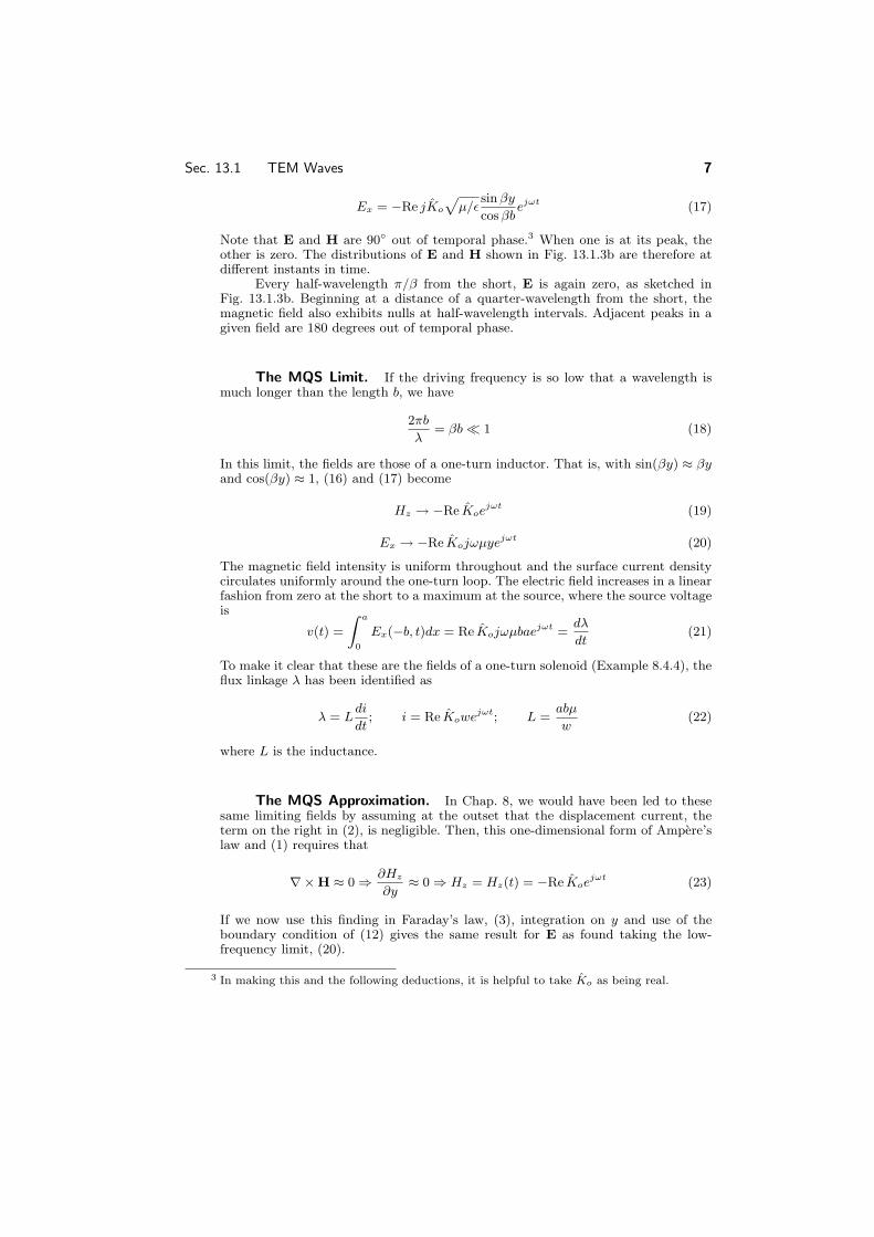
Cite as Markus Zahn course materials for 6641 Electromagnetic Fields Forces and Motion Spring 2005 MIT OpenCourseWare (httpocwmitedu) Massachusetts Institute of Technology Downloaded on [DD Month YYYY]
7 Sec 131 TEM Waves
Ex = minusRe jK o
micro
sin βy ejωt (17)
cos βb
Note that E and H are 90 out of temporal phase3 When one is at its peak the other is zero The distributions of E and H shown in Fig 1313b are therefore at different instants in time
Every halfshywavelength πβ from the short E is again zero as sketched in Fig 1313b Beginning at a distance of a quartershywavelength from the short the magnetic field also exhibits nulls at halfshywavelength intervals Adjacent peaks in a given field are 180 degrees out of temporal phase
The MQS Limit If the driving frequency is so low that a wavelength is much longer than the length b we have
2πb = βb 1 (18)
λ
In this limit the fields are those of a oneshyturn inductor That is with sin(βy) asymp βy and cos(βy) asymp 1 (16) and (17) become
Hz rarr minusRe K oe
jωt (19)
Ex rarr minusRe K ojωmicroyejωt (20)
The magnetic field intensity is uniform throughout and the surface current density circulates uniformly around the oneshyturn loop The electric field increases in a linear fashion from zero at the short to a maximum at the source where the source voltage is
a jωt dλ
v(t) = Ex(minusb t)dx = Re K ojωmicrobae = (21)
dt0
To make it clear that these are the fields of a oneshyturn solenoid (Example 844) the flux linkage λ has been identified as
λ = L di
dt i = Re Kowejωt L =
abmicro
w (22)
where L is the inductance
The MQS Approximation In Chap 8 we would have been led to these same limiting fields by assuming at the outset that the displacement current the term on the right in (2) is negligible Then this oneshydimensional form of Amperersquos law and (1) requires that
partHz times H asymp 0 rArr party
asymp 0 rArr Hz = Hz(t) = minusRe K oe
jωt (23)
If we now use this finding in Faradayrsquos law (3) integration on y and use of the boundary condition of (12) gives the same result for E as found taking the lowshyfrequency limit (20)
3 In making this and the following deductions it is helpful to take K o as being real
8 Electrodynamic Fields The Boundary Value Point of View Chapter 13
Fig 1314 (a) Open circuit transmission line driven by voltage source (b) E and H at times that differ by 90 degrees (c) EQS fields in limit where wavelength is long compared to b
In the previous example the longitudinal boundary conditions (conditions imposed at planes of constant y) could be satisfied exactly using the TEM mode alone The short at the right and the distributed current source at the left each imposed a condition that was like the TEM fields independent of the transverse coordinates In almost all practical situations longitudinal boundary conditions which are independent of the transverse coordinates (used to describe transmission lines) are approximate The open circuit termination at y = 0 shown in Fig 1314 is a case in point as is the source which in this case is not distributed in the x direction
If a longitudinal boundary condition is independent of z the fields are in principle still two dimensional Between the plates we can therefore think of satshyisfying the longitudinal boundary conditions using a superposition of the modes to be developed in the next section These consist of not only the TEM mode conshysidered here but of modes having an x dependence A detailed evaluation of the coefficients specifying the amplitudes of the highershyorder modes brought in by the transverse dependence of a longitudinal boundary condition is illustrated in Sec 133 There we shall find that at low frequencies where these highershyorder modes are governed by Laplacersquos equation they contribute to the fields only in the vicinity of the longitudinal boundaries As the frequency is raised beyond their respective cutoff frequencies the highershyorder modes begin to propagate along the y axis and so have an influence far from the longitudinal boundaries
Here where we wish to restrict ourselves to situations that are well described by the TEM modes we restrict the frequency range of interest to well below the lowest cutoff frequency of the lowest of the highershyorder modes
Given this condition ldquoend effectsrdquo are restricted to the neighborhood of a longitudinal boundary Approximate boundary conditions then determine the disshytribution of the TEM fields which dominate over most of the length In the open
9 Sec 131 TEM Waves
Fig 1315 The surface current density and hence Hz go to zero in the vicinity of the open end
circuit example of Fig 1314a application of the integral charge conservation law to a volume enclosing the end of one of the plates as illustrated in Fig 1315 shows that Ky must be essentially zero at y = 0 For the TEM fields this implies the boundary condition4
Hz(0 t) = 0 (24)
At the left end the vertical segments of perfect conductor joining the voltage source to the parallel plates require that Ex be zero over these segments We shall show later that the highershyorder modes do not contribute to the line integral of E between the plates Thus in so far as the TEM fields are concerned the requirement is that a Vd
Vd(t) = Ex(minusb t)dx Ex(minusb t) = (25) 0
rArr a
Example 1312 Standing Waves on an OpenshyCircuit Parallel Plate Transmission Line
Consider the parallel plates ldquoopenrdquo at y = 0 and driven by a voltage source at y = minusb Boundary conditions are then
Hz(0 t) = 0 Ex(minusb t) = Re Vd ejωta (26)
Evaluation of the coefficients in (10) and (11) so that the boundary conditions in (26) are satisfied gives
VdA+ = minusAminus = minus
2a cos βb
micro (27)
It follows that the TEM fields between the plates (10) and (11) are
Vd sin βy jωt Hz = Re j
micro e (28) a cos βb
Vd cos βy jωt Ex = Re e (29) a cos βb
These distributions of H and E are shown in Fig 1314 at times that differ by 90 degrees The standing wave is similar to that described in the previous example except that it is now E rather than H that peaks at the open end
4 In the region outside the fields are not confined by the plates As a result there is actually some radiation from the open end of the line and this too is not represented by (24) This effect is small if the plate spacing is small compared to a wavelength
10 Electrodynamic Fields The Boundary Value Point of View Chapter 13
The EQS Limit In the low frequency limit where the wavelength is much longer than the length of the plates so that βb 1 the fields given by (28) and (29) become
Vd jωt Hz Re j ωye (30)rarr a
Vd jωt Ex Re e (31)rarr a
At low frequencies the fields are those of a capacitor The electric field is uniform and simply equal to the applied voltage divided by the spacing The magnetic field varies in a linear fashion from zero at the open end to its peak value at the voltage source Evaluation of minusHz at z = minusb gives the surface current density and hence the current i provided by the voltage source
i = Re jω bw
Vdejωt (32) a
Note that this expression implies that
dq bw i = q = CVd C = (33)
dt a
so that the limiting behavior is indeed that of a plane parallel capacitor
EQS Approximation How would the quasistatic fields be predicted in terms of the TEM fields If quasistatic we expect the system to be EQS Thus the magnetic induction is negligible so that the rightshyhand side of (3) is approximated as being equal to zero
partEx times E asymp 0 rArr party
asymp 0 (34)
It follows from integration of this expression and using the boundary condition of (26b) that the quasistatic E is
VdEx = (35)
a
In turn this result provides the displacement current density in Amperersquos law the rightshyhand side of (2)
partHz d Vd
(36)party
dt a
The rightshyhand side of this expression is independent of y Thus integration with respect to y with the ldquoconstantrdquo of integration evaluated using the boundary condition of (26a) gives
d yHz Vd (37)
dt a
For the sinusoidal voltage drive assumed at the outset in the description of the TEM waves this expression is consistent with that found in taking the quasistatic limit (30)
Sec 132 Parallel Plate Modes 11
Demonstration 1311 Visualization of Standing Waves
A demonstration of the fields described by the two previous examples is shown in Fig 1316 A pair of sheet metal electrodes are driven at the left by an oscillator A fluorescent lamp placed between the electrodes is used to show the distribution of the rms electric field intensity
The gas in the tube is ionized by the oscillating electric field Through the fieldshyinduced acceleration of electrons in this gas a sufficient velocity is reached so that collisions result in ionization and an associated optical radiation What is seen is a time average response to an electric field that is oscillating far more rapidly than can be followed by the eye
Because the light is proportional to the magnitude of the electric field the observed 075 m distance between nulls is a halfshywavelength It can be inferred that the generator frequency is f = cλ = 3times 10815 = 200 MHz Thus the frequency is typical of the lower VHF television channels
With the right end of the line shorted the section of the lamp near that end gives evidence that the electric field there is indeed as would be expected from Fig 1313b where it is zero at the short Similarly with the right end open there is a peak in the light indicating that the electric field near that end is maximum This is consistent with the picture given in Fig 1314b In going from an open to a shorted condition the positions of peak light intensity and hence of peak electric field intensity are shifted by λ4
12 Electrodynamic Fields The Boundary Value Point of View Chapter 13
Fig 1321 (a) Plane parallel perfectly conducting plates (b) Coaxial geshyometry in which zshyindependent fields of (a) might be approximately obtained without edge effects
132 TWOshyDIMENSIONAL MODES BETWEEN PARALLEL PLATES
This section treats the boundary value approach to finding the fields between the perfectly conducting parallel plates shown in Fig 1321a Most of the mathematical ideas and physical insights that come from a study of modes on perfectly conducting structures that are uniform in one direction (for example parallel wire and coaxial transmission lines and waveguides in the form of hollow perfectly conducting tubes) are illustrated by this example In the previous section we have already seen that the plates can be used as a transmission line supporting TEM waves In this and the next section we shall see that they are capable of supporting other electromagnetic waves
Because the structure is uniform in the z direction it can be excited in such a way that fields are independent of z One way to make the structure approximately uniform in the z direction is illustrated in Fig 1321b where the region between the plates becomes the annulus of coaxial conductors having very nearly the same radii Thus the difference of these radii becomes essentially the spacing a and the z coordinate maps into the φ coordinate Another way is to make the plates very wide (in the z direction) compared to their spacing a Then the fringing fields from the edges of the plates are negligible In either case the understanding is that the field excitation is uniformly distributed in the z direction The fields are now assumed to be independent of z
Because the fields are two dimensional the classifications and relations given in Sec 126 and summarized in Table 1283 serve as our starting point Cartesian coordinates are appropriate because the plates lie in coordinate planes Fields either have H transverse to the x minus y plane and E in the x minus y plane (TM) or have E transverse and H in the x minus y plane (TE) In these cases Hz and Ez are taken as the functions from which all other field components can be derived We consider sinusoidal steady state solutions so these fields take the form
jωt Hz = Re Hz(x y)e (1) jωt Ez = Re Ez(x y)e (2)
Sec 132 Parallel Plate Modes 13
These field components respectively satisfy the Helmholtz equation (1269) and (12633) in Table 1283 and the associated fields are given in terms of these components by the remaining relations in that table
Once again we find product solutions to the Helmholtz equation where Hz
and Ez are assumed to take the form X(x)Y (y) This formalism for reducing a partial differential equation to ordinary differential equations was illustrated for Helmholtzrsquos equation in Sec 126 This time we take a more mature approach based on the observation that the coefficients of the governing equation are indeshypendent of y (are constants) As a result Y (y) will turn out to be governed by a constant coefficient differential equation This equation will have exponential solushytions Thus with the understanding that ky is a yet to be determined constant (that will turn out to have two values) we assume that the solutions take the specific product forms
H z = h
z(x)eminusjkyy (3)
E z = ez(x)eminusjkyy (4)
Then the field relations of Table 1283 become
TM Fields d2hz 2ˆ+ p hz = 0 (5)dx2
where p2 equiv ω2micro minus k2 y
ky ˆex = minus ω
hz (6)
1 dhz ey = minus
jω dx (7)
TE Fields d2ez 2+ q ez = 0 (8)dx2
where q2 equiv ω2micro minus k2 y
h x =
ky ez (9)
ωmicro
1 dezh
y = jωmicro dx
(10)
The boundary value problem now takes a classic form familiar from Sec 55 What values of p and q will make the electric field tangential to the plates zero For the TM fields ey = 0 on the plates and it follows from (7) that it is the derivative of Hz that must be zero on the plates For the TE fields Ez must itself be zero at the plates Thus the boundary conditions are
TM Fields dh
z (0) = 0 dh
z (a) = 0 (11)dx dx
14 Electrodynamic Fields The Boundary Value Point of View Chapter 13
Fig 1322 Dependence of fundamental fields on x
TE Fields ez(0) = 0 ez(a) = 0 (12)
To check that all of the conditions are indeed met at the boundaries note that if (11) is satisfied there is neither a tangential E nor a normal H at the boundaries for the TM fields (There is no normal H whether the boundary condition is satisfied or not) For the TE field Ez is the only electric field and making Ez=0 on the boundaries indeed guarantees that Hx = 0 there as can be seen from (9)
Representing the TM modes the solution to (5) is a linear combination of sin(px) and cos(px) To satisfy the boundary condition (11) at x = 0 we must select cos(px) Then to satisfy the condition at x = a it follows that p = pn = nπa n = 0 1 2
ˆ (13)hz prop cos pnx
nπ pn = n = 0 1 2 (14)
a
These functions and the associated values of p are called eigenfunctions and eigenshyvalues respectively The solutions that have been found have the x dependence shown in Fig 1322a
From the definition of p given in (5) it follows that for a given frequency ω (presumably imposed by an excitation) the wave number ky associated with the nshyth mode is
ω2micro minus (nπa)2 ω2micro gt (nπa)2
ky equiv plusmnβn βn equiv minusj
(nπa)2 minus ω2micro ω2micro lt (nπa)2 (15)
Similar reasoning identifies the modes for the TE fields Of the two solutions to (8) the one that satisfies the boundary condition at x = 0 is sin(qx) The second boundary condition then requires that q take on certain eigenvalues qn
ez prop sin qnx (16)
nπ qn = (17)
a
Sec 132 Parallel Plate Modes 15
The x dependence of Ez is then as shown in Fig 1322b Note that the case n = 0 is excluded because it implies a solution of zero amplitude
For the TE fields it follows from (17) and the definition of q given with (8) that5
ω2micro minus (nπa)2 ω2micro gt (nπa)2 ky equiv plusmnβn βn equiv minusj
(nπa)2 minus ω2micro ω2micro lt (nπa)2
(18)
In general the fields between the plates are a linear combination of all of the modes In superimposing these modes we recognize that ky = plusmnβn Thus with coefficients that will be determined by boundary conditions in planes of constant y we have the solutions
TM Modes
eminusjβoy + Aminus jβoyHz =Re A+
o o e infin
eminusjβny + Aminus nπ jωt (19)
+
A+ n n e
jβny cos x
e
a n=1
TE Modes
infin
eminusjβny + Cminusenπ jωt Ez = Re
Cn
+ n
jβny sin x e (20)
a n=1
We shall refer to the nshyth mode represented by these fields as the TMn or TEn
mode respectively We now make an observation about the TM0 mode that is of farshyreaching
significance Its distribution of Hz has no dependence on x [(13) with pn = 0] As a result Ey = 0 according to (7) Thus for the TM0 mode both E and H are transverse to the axial direction y This special mode represented by the n = 0 terms in (19) is therefore the transverse electromagnetic (TEM) mode featured in the previous section One of its most significant features is that the relation between frequency ω and wave number in the y direction ky [(15) with n = 0] is ky = plusmnω
radicmicro = plusmnωc the same as for a uniform electromagnetic plane wave
Indeed as we saw in Sec 131 it is a uniform plane wave The frequency dependence of ky for the TEM mode and for the highershyorder
TMn modes given by (15) are represented graphically by the ω minus ky plot of Fig 1323 For a given frequency ω there are two values of ky which we have called plusmnβn The dashed curves represent imaginary values of ky Imaginary values correspond to exponentially decaying and ldquogrowingrdquo solutions An exponentially ldquogrowingrdquo solution is in fact a solution that decays in the minusy direction Note that the switch from exponentially decaying to propagating fields for the highershyorder modes occurs at the cutoff frequency
1 nπ ωcn = radic
micro a
(21)
5 For the particular geometry considered here it has turned out that the eigenvalues pn and qn are the same (with the exception of n = 0) This coincidence does not occur with boundaries having other geometries
16 Electrodynamic Fields The Boundary Value Point of View Chapter 13
Fig 1323 Dispersion relation for TM modes
Fig 1324 Dispersion relation for TE modes
The velocity of propagation of points of constant phase (for example a point at which a field component is zero) is ωky Figure 1323 emphasizes that for all but the TEM mode the phase velocity is a function of frequency The equation relating ω to ky represented by this figure (15) is often called the dispersion equation
The dispersion equation for the TE modes is shown in Fig 1324 Although the field distributions implied by each branch are very different in the case of the plane parallel electrodes considered here the curves are the same as those for the TMn=0 modes
The next section will provide greater insight into the highershyorder TM and TE modes
Sec 133 TE and TM Standing Waves 17
133 TE AND TM STANDING WAVES BETWEEN PARALLEL PLATES
In this section we delve into the relationship between the twoshydimensional highershyorder modes derived in Sec 132 and their sources The examples are chosen to relate directly to case studies treated in quasistatic terms in Chaps 5 and 8
The matching of a longitudinal boundary condition by a superposition of modes may at first seem to be a purely mathematical process However even qualishytatively it is helpful to think of the influence of an excitation in terms of the resulting modes For quasistatic systems this has already been our experience For the purshypose of estimating the dependence of the output signal on the spacing b between excitation and detection electrodes the EQS response of the capacitive attenuator of Sec 55 could be pictured in terms of the lowestshyorder mode In the electrodyshynamic situations of interest here it is even more common that one mode dominates Above its cutoff frequency a given mode can propagate through a waveguide to reshygions far removed from the excitation
Modes obey orthogonality relations that are mathematically useful for the evaluation of the mode amplitudes Formally the mode orthogonality is implied by the differential equations governing the transverse dependence of the fundamental field components and the associated boundary conditions For the TM modes these are (1325) and (13211)
TM Modes d2hzn + p 2nh
zn = 0 (1)dx2
where dh
zn (a) = 0 dhzn (0) = 0
dx dx
and for the TE modes these are (1328) and (13212)
TE Modes d2ezn + qn
2 ezn = 0 (2)dx2
where ezn(a) = 0 ezn(0) = 0
The word ldquoorthogonalrdquo is used here to mean that
a ˆ ˆhznhzmdx = 0 n = m (3)
0
a
eznezmdx = 0 n = m (4) 0
These properties of the modes can be seen simply by carrying out the integrals using the modes as given by (13213) and (13216) More fundamentally they can be deduced from the differential equations and boundary conditions themselves (1) and (2) This was illustrated in Sec 55 using arguments that are directly applicable here [(5520)ndash(5526)]
18 Electrodynamic Fields The Boundary Value Point of View Chapter 13
Fig 1331 Configuration for excitation of TM waves
The following two examples illustrate how TE and TM modes can be excited in waveguides In the quasistatic limit the configurations respectively become identical to EQS and MQS situations treated in Chaps 5 and 8
Example 1331 Excitation of TM Modes and the EQS Limit
In the configuration shown in Fig 1331 the parallel plates lying in the planes x = 0 and x = a are shorted at y = 0 by a perfectly conducting plate The excitation is provided by distributed voltage sources driving a perfectly conducting plate in the plane y = b These sources constrain the integral of E across narrow insulating gaps of length Δ between the respective edges of the upper plate and the adjacent plates All the conductors are modeled as perfect The distributed voltage sources maintain the twoshydimensional character of the fields even as the width in the z direction becomes long compared to a wavelength Note that the configuration is identical to that treated in Sec 55 Therefore we already know the field behavior in the quasistatic (low frequency) limit
In general the twoshydimensional fields are the sum of the TM and TE fields However here the boundary conditions can be met by the TM fields alone Thus we begin with Hz (13219) expressed as a single sum
(A+ eminusjβny jβny nπ jωt Hz = Re
infin
n + Aminusn e ) cos xe (5)
a n=0
This field and the associated E satisfy the boundary conditions on the parallel plates at x = 0 and x = a Boundary conditions are imposed on the tangential E at the longitudinal boundaries where y = 0
Ex(x 0 t) = 0 (6)
Sec 133 TE and TM Standing Waves 19
and at the driving electrode where y = b We assume here that the gap lengths Δ are small compared to other dimensions of interest Then the electric field within each gap is conservative and the line integral of Ex across the gaps is equal to the gap voltages plusmnv Over the region between x = Δ and x = a minus Δ the perfectly conducting electrode makes Ex = 0
a Δ Ex(x b t)dx = v Ex(x b t)dx = minusv (7)
aminusΔ 0
Because the longitudinal boundary conditions are on Ex we substitute Hz
as given by (5) into the x component of Faradayrsquos law [(1266) of Table 1283] to obtain
infin minusβn (A+ eminusjβny minus Aminuse
nπ jωt Ex = Re
n n jβny
cos x
e (8)
ω a n=0
To satisfy the condition at the short (6) A+ = nn Aminus and (8) becomes
2jβn A+ nπ jωt Ex = Re
infinn sin βny cos x
e (9)
ω a n=0
This set of solutions satisfies the boundary conditions on three of the four boundaries What we now do to satisfy the ldquolastrdquo boundary condition differs little from what was done in Sec 55 The A+rsquos are adjusted so that the summation ofn
product solutions in (9) matches the boundary condition at y = b summarized by (7) Thus we write (9) with y = b on the right and with the function representing (7) on the left This expression is multiplied by the mrsquoth eigenfunction cos(mπxa) and integrated from x = 0 to x = a
a a infin n
E
x(x b) cos mπx
dx = 2jβnA+
sin βnb a ω
middot 0 0 n=0 (10)
nπ mπ cos x cos xdx
a a
Because the intervals where E x(x b) is finite are so small the cosine function can
be approximated by a constant namely plusmn1 as appropriate On the rightshyhand side of (10) we exploit the orthogonality condition so as to pick out only one term in the infinite series
v[minus1 + cos mπ] =2jβm
sin βmb a
A+ (11)ω 2
m
Of the infinite number of terms in the integral on the right in (10) only the term where n = m has contributed The coefficients follow from solving (11) and replacing m nrarr
0 n evenA+ minus2ωv
n = n odd (12) jβna sin βnb
20 Electrodynamic Fields The Boundary Value Point of View Chapter 13
With the coefficients A+ = Aminus now determined we can evaluate all of the n n
fields Substitution into (5) and (8) and into the result using (1267) from Table 1283 gives infin
4jωv cos βny nπ
jωtHz = Re
cos x e (13)βna sin βnb a
n=1 odd
infin minus4ˆ v sin βny nπ
jωt Ex = Re
cos x e (14) a sin βnb a
n=1 odd
infin 4nπ v cos βny nπ
jωt Ey = Re
sin x e (15)
a (βna) sin βnb a n=1 odd
Note the following aspects of these fields (which we can expect to see in Demonshystration 1331) First the magnetic field is directed perpendicular to the xminusy plane Second by making the excitation symmetric we have eliminated the TEM mode As a result the only modes are of order n = 1 and higher Third at frequencies below the cutoff for the TM1 mode βy is imaginary and the fields decay in the y direction6 Indeed in the quasistatic limit where ω2micro (πa)2 the electric field is the same as that given by taking the gradient of (559) In this same quasistatic limit the magnetic field would be obtained by using this quasistatic E to evaluate the displacement current and then solving for the resulting magnetic field subject to the boundary condition that there be no normal flux density on the surfaces of the perfect conductors Fourth above the cutoff frequency for the n = 1 mode but below the cutoff for the n = 2 mode we should find standing waves having a wavelength 2πβ1
Finally note that each of the expressions for the field components has sin(βnb) in its denominator With the frequency adjusted such that βn = nπb this function goes to zero and the fields become infinite This resonance condition results in an infinite response because we have pictured all of the conductors as perfect It occurs when the frequency is adjusted so that a wave reflected from one boundary arrives at the other with just the right phase to reinforce upon a second reflection the wave currently being initiated by the drive
The following experiment gives the opportunity to probe the fields that have been found in the previous example In practical terms the structure considered might be a parallel plate waveguide
Demonstration 1331 Evanescent and Standing TM Waves
The experiment shown in Fig 1332 is designed so that the field distributions can be probed as the excitation is varied from below to above the cutoff frequency of the TM1 mode The excitation structures are designed to give fields approximating those found in Example 1331 For convenience a = 48 cm so that the excitation frequency ranges above and below a cutshyoff frequency of 31 GHz The generator is modulated at an audible frequency so that the amplitude of the detected signal is converted to ldquoloudnessrdquo of the tone from the loudspeaker
In this TM case the driving electrode is broken into segments each insulated from the parallel plates forming the waveguide and each attached at its center to a
6 sin(ju) = j sinh(u) and cos(ju) = cosh(u)
Sec 133 TE and TM Standing Waves 21
Fig 1332 Demonstration of TM evanescent and standing waves
coaxial line from the generator The segments insure that the fields applied to each part of the electrode are essentially in phase (The cables feeding each segment are of the same length so that signals arrive at each segment in phase) The width of the structure in the z direction is of the order of a wavelength or more to make the fields two dimensional (Remember in the vicinity of the lowest cutoff frequency a is about oneshyhalf wavelength) Thus if the feeder were attached to a contiguous electrode at one point there would be a tendency for standing waves to appear on the excitation electrode much as they did on the wire antennae in Sec 124 In the experiment the segments are about a quartershywavelength in the z direction but of course about a halfshywavelength in the x direction
In the experiment H is detected by means of a oneshyturn coil The voltage induced at the terminals of this loop is proportional to the magnetic flux perpendicshyular to the loop Thus for the TM fields the loop detects its greatest signal when it is placed in an x minus y plane To avoid interference with E the coaxial line connected to the probe as well as the loop itself are kept adjacent to the conducting walls (where Hz peaks anyway)
The spatial features of the field implied by the normalized ω versus ky plot of Fig 1332 can be seen by moving the probe about With the frequency below cutoff the field decays in the minusy direction This exponential decay or evanescence decreases to a linear dependence at cutoff and is replaced above cutoff by standing waves The value of ky at a given frequency can be deduced from the experiment by measuring the quartershywave distance from the short to the first null in the magnetic field Note that if there are asymmetries in the excitation that result in excitation of the TEM mode the standing waves produced by this mode will tend to obscure
Cite as Markus Zahn course materials for 6641 Electromagnetic Fields Forces and Motion Spring 2005 MIT OpenCourseWare (httpocwmitedu) Massachusetts Institute of Technology Downloaded on [DD Month YYYY]
22 Electrodynamic Fields The Boundary Value Point of View Chapter 13
the TM1 mode when it is evanescent The TEM waves do not have a cutoff
As we have seen once again the TM fields are the electrodynamic generalizashytion of twoshydimensional EQS fields That is in the quasistatic limit the previous example becomes the capacitive attenuator of Sec 557
We have more than one reason to expect that the twoshydimensional TE fields are the generalization of MQS systems First this was seen to be the case in Sec 126 where the TE fields associated with a given surface current density were found to approach the MQS limit as ω2micro k2 Second from Sec 86 we know ythat for every twoshydimensional EQS configuration involving perfectly conducting boundaries there is an MQS one as well8 In particular the MQS analog of the capacitor attenuator is the configuration shown in Fig 1333 The MQS H field was found in Example 863
In treating MQS fields in the presence of perfect conductors we recognized that the condition of zero tangential E implied that there be no timeshyvarying normal B This made it possible to determine H without regard for E We could then delay taking detailed account of E until Sec 101 Thus in the MQS limit a system involving essentially a twoshydimensional distribution of H can (and usually does) have an E that depends on the third dimension For example in the configuration of Fig 1333 a voltage source might be used to drive the current in the z direction through the upper electrode This current is returned in the perfectly conducting shyshaped walls The electric fields in the vicinities of the gaps must therefore increase in the z direction from zero at the shorts to values consistent with the voltage sources at the near end Over most of the length of the system E is across the gap and therefore in planes perpendicular to the z axis This MQS configuration does not excite pure TE fields In order to produce (approximately) twoshydimensional TE fields provision must be made to make E as well as H two dimensional The following example and demonstration give the opportunity to further develop an appreciation for TE fields
Example 1332 Excitation of TE Modes and the MQS Limit
An idealized configuration for exciting standing TE modes is shown in Fig 1334 As in Example 1331 the perfectly conducting plates are shorted in the plane y = 0 In the plane y = b is a perfectly conducting plate that is segmented in the z direction Each segment is driven by a voltage source that is itself distributed in the x direction In the limit where there are many of these voltage sources and perfectly conducting segments the driving electrode becomes one that both imposes a zshydirected E and has no z component of B That is just below the surface of this electrode wEz is equal to the sum of the source voltages One way of approximately realizing this idealization is used in the next demonstration
Let Λ be defined as the flux per unit length (length taken along the z direction) into and out of the enclosed region through the gaps of width Δ between the driving electrode and the adjacent edges of the plane parallel electrodes The magnetic field
7 The example which was the theme of Sec 55 might equally well have been called the ldquomicrowave attenuatorrdquo for a section of waveguide operated below cutoff is used in microwave circuits to attenuate signals
8 The H satisfying the condition that n B = 0 on the perfectly conducting boundaries was middot obtained by replacing Φ Az in the solution to the analogous EQS problem rarr
Cite as Markus Zahn course materials for 6641 Electromagnetic Fields Forces and Motion Spring 2005 MIT OpenCourseWare (httpocwmitedu) Massachusetts Institute of Technology Downloaded on [DD Month YYYY]
Sec 133 TE and TM Standing Waves 23
Fig 1333 Twoshydimensional MQS configuration that does not have TEfields
Fig 1334 Idealized configuration for excitation of TE standing waves
normal to the driving electrode between the gaps is zero Thus at the upper surface Hy has the distribution shown in Fig 1335a
Faradayrsquos integral law applied to the contour C of Fig 1334 and to a similar contour around the other gap shows that
Ez(x b t) = minus d
dt
Λ rArr E z = minusjωΛ (16)
24 Electrodynamic Fields The Boundary Value Point of View Chapter 13
Fig 1335 Equivalent boundary conditions on normal H and tanshygential E at y = b
Thus either the normal B or the tangential E on the surface at y = b is specified The two must be consistent with each other ie they must obey Faradayrsquos law It is perhaps easiest in this case to deal directly with Ez in finding the coefficients apshypearing in (13220) Once they have been determined (much as in Example 1331) H follows from Faradayrsquos law (12629) and (12630) of Table 1283
infin 4jΛω sin βmy mπx jωtEz = Re sin e (17)
minus
mπ sin βmb a m=1 odd
infin 4βmΛ cos βmy mπx jωt Hx = Re
sin e (18)
micromπ sin βmb a m=1 odd
infin Λ sin βmy mπx jωt Hy = Re
minus4ˆcos e (19)
microa sin βmb a m=1 odd
In the quasistatic limit ω2micro (mπa)2 this magnetic field reduces to that found in Example 863
A few observations may help one to gain some insights from these expressions First if the magnetic field is sensed then the detection loop must have its axis in the xminus y plane For these TE modes there should be no signal sensed with the axis of the detection loop in the z direction This probe can also be used to verify that H normal to the perfectly conducting surfaces is indeed zero while its tangential value peaks at the short Second the same decay of the fields below cutoff and appearance of standing waves above cutoff is predicted here as in the TM case Third because E is perpendicular to planes of constant z the boundary conditions on E and hence H are met even if perfectly conducting plates are placed over the open ends of the guide say in the planes z = 0 and z = w In this case the guide becomes a closed pipe of rectangular crossshysection What we have found are then a subset of the threeshydimensional modes of propagation in a rectangular waveguide
Demonstration 1332 Evanescent and Standing TE Waves
The apparatus of Demonstration 1331 is altered to give TE rather than TM waves by using an array of ldquooneshyturn inductorsrdquo rather than the array of ldquocapacitor platesrdquo These are shown in Fig 1336
Sec 134 Rectangular Waveguide Modes 25
Fig 1336 Demonstration of evanescent and standing TE waves
Each member of the array consists of an electrode of width a minus 2Δ driven at one edge by a common source and shorted to the perfectly conducting backing at its other edge Thus the magnetic flux through the closed loop passes into and out of the guide through the gaps of width Δ between the ends of the oneshyturn coil and the parallel plate (vertical) walls of the guide Effectively the integral of Ez created by the voltage sources in the idealized model of Fig 1334 is produced by the integral of Ez between the left edge of one current loop and the right edge of the next
The current loop can be held in the x minus z plane to sense Hy or in the y minus z plane to sense Hx to verify the field distributions derived in the previous example It can also be observed that placing conducting sheets against the open ends of the parallel plate guide making it a rectangular pipe guide leaves the characteristics of these twoshydimensional TE modes unchanged
134 RECTANGULAR WAVEGUIDE MODES
Metal pipe waveguides are often used to guide electromagnetic waves The most common waveguides have rectangular crossshysections and so are well suited for the exploration of electrodynamic fields that depend on three dimensions Although we confine ourselves to a rectangular crossshysection and hence Cartesian coordinates the classification of waveguide modes and the general approach used here are equally applicable to other geometries for example to waveguides of circular crossshysection
The parallel plate system considered in the previous three sections illustrates
Cite as Markus Zahn course materials for 6641 Electromagnetic Fields Forces and Motion Spring 2005 MIT OpenCourseWare (httpocwmitedu) Massachusetts Institute of Technology Downloaded on [DD Month YYYY]
26 Electrodynamic Fields The Boundary Value Point of View Chapter 13
Fig 1341 Rectangular waveguide
much of what can be expected in pipe waveguides However unlike the parallel plates which can support TEM modes as well as highershyorder TE modes and TM modes the pipe cannot transmit a TEM mode From the parallel plate system we expect that a waveguide will support propagating modes only if the frequency is high enough to make the greater interior crossshysectional dimension of the pipe greater than a free space halfshywavelength Thus we will find that a guide having a larger dimension greater than 5 cm would typically be used to guide energy having a frequency of 3 GHz
We found it convenient to classify twoshydimensional fields as transverse magshynetic (TM) or transverse electric (TE) according to whether E or H was transshyverse to the direction of propagation (or decay) Here where we deal with threeshydimensional fields it will be convenient to classify fields according to whether they have E or H transverse to the axial direction of the guide This classification is used regardless of the crossshysectional geometry of the pipe We choose again the y coordinate as the axis of the guide as shown in Fig 1341 If we focus on solutions to Maxwellrsquos equations taking the form
Hy = Re hy(x z)ej(ωtminuskyy) (1)
Ey = Re ey(x z)ej(ωtminuskyy) (2)
then all of the other complex amplitude field components can be written in terms of the complex amplitudes of these axial fields Hy and Ey This can be seen from substituting fields having the form of (1) and (2) into the transverse components of Amperersquos law (1208)
minusjkyhz minus parth
y = jωex (3)partz
Sec 134 Rectangular Waveguide Modes 27
parth y + jkyh
x = jωez (4)partx
and into the transverse components of Faradayrsquos law (1209)
minusjky ez minus partey = minusjωmicrohx (5)partz
partey + jky ex = minusjωmicrohz (6)partx
If we take h y and ˆ ey as specified (3) and (6) constitute two algebraic equations in
the unknowns ˆ ex and h z Thus they can be solved for these components Similarly
h x and ez follow from (4) and (5)
parth
y partey
h
x = minus jky partx
minus jω (ω2micro minus k2) (7)partz y
h z =
minus jky parth
y + jω partey
(ω2micro minus k2) (8)
partz partx y
ex =
jωmicro parth
y minus jky partey
(ω2micro minus ky
2) (9)partz partx
parthy partˆ ez =
minus jωmicropartx
minus jky ey
(ω2micro minus ky
2) (10)partz
We have found that the threeshydimensional fields are a superposition of those associated with Ey (so that the magnetic field is transverse to the guide axis ) the TM fields and those due to Hy the TE modes The axial field components now play the role of ldquopotentialsrdquo from which the other field components can be derived
We can use the y components of the laws of Ampere and Faraday together with Gaussrsquo law and the divergence law for H to show that the axial complex amplitudes ˆ ey and h
y satisfy the twoshydimensional Helmholtz equations
TM Modes (Hy = 0)
part2ey
partx2 +
part2ey
partz2 + p 2 ey = 0 (11)
where 2 p = ω2micro minus k2
y
and
TE Modes (Ey = 0)
part2hy part2h y+ + q 2h
y = 0 (12)partx2 partz2
28 Electrodynamic Fields The Boundary Value Point of View Chapter 13
where q 2 = ω2micro minus ky
2
These relations also follow from substitution of (1) and (2) into the y components of (1302) and (1301)
The solutions to (11) and (12) must satisfy boundary conditions on the pershyfectly conducting walls Because Ey is parallel to the perfectly conducting walls it must be zero there
TM Modes
ey(0 z) = 0 ey(a z) = 0 ey(x 0) = 0 ey(xw) = 0 (13)
The boundary condition on Hy follows from (9) and (10) which express ex
and ˆ ez in terms of h y On the walls at x = 0 and x = a ez = 0 On the walls at
z = 0 z = w ex = 0 Therefore from (9) and (10) we obtain
TE Modes
parthy (0 z) = 0 parthy (a z) = 0
parthy (x 0) = 0 parthy (x w) = 0 (14)
partx partx partz partz
The derivative of hy with respect to a coordinate perpendicular to the boundary must be zero
The solution to the Helmholtz equation (11) or (12) follows a pattern that is familiar from that used for Laplacersquos equation in Sec 54 Either of the complex amplitudes representing the axial fields is represented by a product solution
ey
ˆ prop X(x)Z(z) (15)hy
Substitution into (11) or (12) and separation of variables then gives
d2X + γ2X = 0 (16)
dx2
d2Z + δ2Z = 0
dz2
where
minusγ2 minus δ2 +
p2
2
= 0 (17)q
Solutions that satisfy the TM boundary conditions (13) are then
TM Modes
mπ X prop sin γmx γm = m = 1 2 (18)
a
29 Sec 134 Rectangular Waveguide Modes
nπ Z prop sin δnz δn = n = 1 2
w
so that pmn 2 =
mπ 2 + nπ 2 m = 1 2 n = 1 2 (19)
a w
When either m or n is zero the field is zero and thus m and n must be equal to an integer equal to or greater than one For a given frequency ω and mode number (mn) the wave number ky is found by using (19) in the definition of p associated with (11)
ky = plusmnβmn
with ⎧ ω2micro minus
mπ
2 minus
nπ 2 2 +
nπ
2⎨ w ω2micro gt
mπ
w (20)βmna a equiv ⎩ minusj
mπ
2 +
nπ 2 minus ω2micro ω2micro lt
mπ
2 +
nπ 2
a w a w
Thus the TM solutions are
infin infin mπ nπ
Ey = Re
(A+ eminusjβmn y + Aminus ejβmn y) sin x sin z ejωt (21)mn mn a w m=1 n=1
For the TE modes (14) provides the boundary conditions and we are led to the solutions
TE Modes
mπ X prop cos γmx γm = m = 0 1 2 (22)
a
nπ Z prop cos δnz δn = n = 0 1 2
a
Substitution of γm and δn into (17) therefore gives
q 2 = mπ 2 +
nπ 2 m = 0 1 2 n = 0 1 2 (23)mn a w
(mn) = (0 0)
The wave number ky is obtained using this eigenvalue in the definition of q assoshyciated with (12) With the understanding that either m or n can now be zero the expression is the same as that for the TM modes (20) However both m and n cannot be zero If they were it follows from (22) that the axial H would be uniform over any given crossshysection of the guide The integral of Faradayrsquos law over the crossshysection of the guide with the enclosing contour C adjacent to the perfectly conducting boundaries as shown in Fig 1342 requires that
E ds = minusmicroA
dHy (24)middot dt
30 Electrodynamic Fields The Boundary Value Point of View Chapter 13
Fig 1342 Crossshysection of guide with contour adjacent to perfectly conshyducting walls
where A is the crossshysectional area of the guide Because the contour on the left is adjacent to the perfectly conducting boundaries the line integral of E must be zero It follows that for the m = 0 n = 0 mode Hy = 0 If there were such a mode it would have both E and H transverse to the guide axis We will show in Sec 142 where TEM modes are considered in general that TEM modes cannot exist within a perfectly conducting pipe
Even though the dispersion equations for the TM and TE modes only differ in the allowed lowest values of (mn) the field distributions of these modes are very different9 The superposition of TE modes gives
infin infin mπ nπ
Re
(C+ eminusjβmn y + Cminus jβmn y) jωt Hy = mn mne cos x cos z e (25) a w
middot m=0 n=0
where m n = 0 The frequency at which a given mode switches from evanescence middot to propagation is an important parameter This cutoff frequency follows from (20) as
1 mπ 2 +
nπ 2 ωc = radic
micro a w (26)
TM Modes m = 0 n = 0
TE Modes m and n not both zero
Rearranging this expression gives the normalized cutoff frequency as functions of the aspect ratio aw of the guide
ωcw ωc equiv
cπ =
(wa)2m2 + n2 (27)
These normalized cutoff frequencies are shown as functions of wa in Fig 1343 The numbering of the modes is standardized The dimension w is chosen as
w le a and the first index m gives the variation of the field along a The TE10
9 In other geometries such as a circular waveguide this coincidence of pmn and qmn is not found
Sec 134 Rectangular Waveguide Modes 31
Fig 1343 Normalized cutoff frequencies for lowest rectangular waveguide modes as a function of aspect ratio
mode then has the lowest cutoff frequency and is called the dominant mode All other modes have higher cutoff frequencies (except of course in the case of the square crossshysection for which TE01 has the same cutoff frequency) Guides are usually designed so that at the frequency of operation only the dominant mode is propagating while all highershyorder modes are ldquocutoffrdquo
In general an excitation of the guide at a crossshysection y = constant excites all waveguide modes The modes with cutoff frequencies higher than the frequency of excitation decay away from the source Only the dominant mode has a sinusoidal dependence upon y and thus possesses fields that are periodic in y and ldquodominaterdquo the field pattern far away from the source at distances larger than the transverse dimensions of the waveguide
Example 1341 TE10 Standing Wave Fields
The section of rectangular guide shown in Fig 1344 is excited somewhere to the right of y = 0 and shorted by a conducting plate in the plane y = 0 We presume that the frequency is above the cutoff frequency for the TE10 mode and that a gt w as shown The frequency of excitation is chosen to be below the cutoff frequency for all higher order modes and the source is far away from y = 0 (ie at y a) The field in the guide is then that of the TE10 mode Thus Hy is given by (25) with m = 1 and n = 0 What is the spaceshytime dependence of the standing waves that result from having shorted the guide
Because of the short Ez(x y = 0 z) = 0 In order to relate the coefficients
C+ and Cminus we must determine ˆ ez from h y as given by (25) using (10) 10 10
a 10e
minusjβ10y jβ10y πx jωt 10eEz = Re jωmicro (C+ + Cminus ) sin e (28)
π a
and because ez = 0 at the short it follows that
C+ = minusCminus (29)10 10
32 Electrodynamic Fields The Boundary Value Point of View Chapter 13
Fig 1344 Fields and surface sources for TE10 mode
so that a π jωt
Ez = 2ωmicro C+ xe (30)Re 10 sin β10y sin
π a
and this is the only component of the electric field in this mode We can now use (29) to evaluate (25)
π jωt
Hy = minusRe 2jC+ cos xe (31)10 sin β10y
a
In using (7) to evaluate the other component of H remember that in the C+ termmn
of (25) ky = βmn while in the Cminus term ky = minusβmnmn
a π jωt
C+Hx = Re 2jβ10 10 cos β10y sin xe (32)
π a
To sketch these fields in the neighborhood of the short and deduce the associshyated surface charge and current densities consider C+ to be real The j in (31) and 10
(32) shows that Hx and Hy are 90 degrees out of phase with the electric field Thus in the field sketches of Fig 1344 E and H are shown at different instants of time say E when ωt = π and H when ωt = π2 The surface charge density is where Ez
terminates and originates on the upper and lower walls The surface current density can be inferred from Amperersquos continuity condition The temporal oscillations of these fields should be pictured with H equal to zero when E peaks and with E equal to zero when H peaks At planes spaced by multiples of a halfshywavelength along the y axis E is always zero
Sec 135 Optical Fibers 33
Fig 1345 Slotted line for measuring axial distribution of TE10 fields
The following demonstration illustrates how a movable probe designed to coushyple to the electric field is introduced into a waveguide with minimal disturbance of the wall currents
Demonstration 1341 Probing the TE10 Mode
A waveguide slotted line is shown in Fig 1345 Here the line is shorted at y = 0 and excited at the right The probe used to excite the guide is of the capacitive type positioned so that charges induced on its tip couple to the lines of electric field shown in Fig 1344 This electrical coupling is an alternative to the magnetic coupling used for the TE mode in Demonstration 1332
The y dependence of the field pattern is detected in the apparatus shown in Fig 1345 by means of a second capacitive electrode introduced through a slot so that it can be moved in the y direction and not perturb the field ie the wall is cut along the lines of the surface current K From the sketch of K given in Fig 1344 it can be seen that K is in the y direction along the center line of the guide
The probe can be used to measure the wavelength 2πky of the standing waves by measuring the distance between nulls in the output signal (between nulls in Ez) With the frequency somewhat below the cutoff of the TE10 mode the spatial decay away from the source of the evanescent wave also can be detected
135 DIELECTRIC WAVEGUIDES OPTICAL FIBERS
Waves can be guided by dielectric rods or slabs and the fields of these waves occupy the space within and around these dielectric structures Especially at optical wavelengths dielectric fibers are commonly used to guide waves In this section we develop the properties of waves guided by a planar sheet of dielectric material The waves that we find are typical of those found in integrated optical systems and in the more commonly used optical fibers of circular crossshysection
A planar version of a dielectric waveguide is pictured in Fig 1351 A dielectric of thickness 2d and permittivity i is surrounded by a dielectric of permittivity lt i The latter might be free space with = o We are interested in how this
34 Electrodynamic Fields The Boundary Value Point of View Chapter 13
Fig 1351 Dielectric slab waveguide
structure might be used to guide waves in the y direction and will confine ourselves to fields that are independent of z
With a source somewhere to the left (for example an antenna imbedded in the dielectric) there is reason to expect that there are fields outside as well as inside the dielectric We shall look for field solutions that propagate in the y direction and possess fields solely inside and near the layer The fields external to the layer decay to zero in the plusmnx directions Like the waves propagating along waveguides those guided by this structure have transverse components that take the form
Ez = Re ˆ ez(x)ej(ωtminuskyy) (1)
both inside and outside the dielectric That is the fields inside and outside the dielectric have the same frequency ω the same phase velocity ωky and hence the same wavelength 2πky in the y direction Of course whether such fields can actually exist will be determined by the following analysis
The classification of twoshydimensional fields introduced in Sec 126 is applicashyble here The TM and TE fields can be made to independently satisfy the boundary conditions so that the resulting modes can be classified as TM or TE10 Here we will confine ourselves to the transverse electric modes In the exterior and interior regions where the permittivities are uniform but different it follows from substishytution of (1) into (12633) (Table 1283) that
d2ez minus α2 xez = 0 αx =
ky
2 minus ω2micro d lt x and x lt minusd (2)dx2
d2ez + k2 ez = 0 kx =
ω2microi minus k2 minusd lt x lt d (3)dx2 x y
A guided wave is one that is composed of a nonuniform plane wave in the exterior regions decaying in the plusmnx directions and propagating with the phase velocity ωky in the y direction In anticipation of this we have written (2) in
10 Circular dielectric rods do not support simple TE or TM waves in that case this classifishycation of modes is not possible
Sec 135 Optical Fibers 35
terms of the parameter αx which must then be real and positive Through the continuity conditions the exterior wave must match up to the interior wave at the dielectric surfaces The solutions to (3) are sines and cosines if kx is real In order to match the interior fields onto the nonuniform plane waves on both sides of the guide it is necessary that kx be real
We now set out to find the wave numbers ky that not only satisfy the wave equations in each of the regions represented by (2) and (3) but the continuity conditions at the interfaces as well The configuration is symmetric about the x = 0 plane so we can further divide the modes into those that have even and odd functions Ez(x) Thus with A an arbitrary factor appropriate even solutions to (2) and (3) are ⎧
⎪⎪⎨
⎪⎪⎩
Aeminusαx(xminusd) d lt x cos kxx
ez = A minusd lt x lt d (4)cos kxd
Aeαx(x+d) x lt minusd
To simplify the algebra we have displaced the origin in the exterior solutions so that just the coefficient A is obtained when ez is evaluated at the respective interfaces With a similar objective the interior solution has been divided by the constant cos(kxd) so that at the boundaries ez also becomes A In this way we have adjusted the interior coefficient so that ez is continuous at the boundaries
Because this transverse field is the only component of E all of the continuity conditions on E are now satisfied The permeabilities of all regions are presumed to be the same so both tangential and normal components of H must be continuous at the boundaries From (12629) the continuity of normal microH is guaranteed by the continuity of Ez in any case The tangential field is obtained using (12630)
h y =
1 dez (5)jωmicro dx
Substitution of (4) into (5) gives
hy = 1
jωmicro
⎧⎨
⎩
minusα Aeminusαx(xminusd) d lt x minusk
x
A sin kxx minusd lt x lt d (6)cos kxdx
αxAeαx(x+d) x lt minusd
The assumption that Ez is even in x has as a consequence the fact that the continushyity condition on tangential H is satisfied by the same relation at both boundaries
αx minusαxA = minuskxA tan kxd rArr kx
= tan kxd (7)
Our goal is to determine the propagation constant ky for a given ω If we were to substitute the definitions of αx and kx into this expression we would have this dispersion equation D(ωky) implicitly relating ky to ω It is more convenient to solve for αx and kx first and then for ky
Elimination of ky between the expressions for αx and kx given with (2) and (3) gives a second expression for αxkx
αx =
ω2microid2
1minus minus 1 (8)
kx (kxd)2 i
36 Electrodynamic Fields The Boundary Value Point of View Chapter 13
Fig 1352 Graphical solution to (7) and (8)
The solutions for the values of the normalized transverse wave numbers (kxd) can be pictured as shown in Fig 1352 Plotted as functions of kxd are the rightshyhand sides of (7) and (8) The points of intersection kxd = γm are the desired solutions For the frequency used to make Fig 1352 there are two solutions These are designated by even integers because the odd modes (Prob 1351) have roots that interleave these even modes
As the frequency is raised an additional even TEshyguided mode is found each time the curve representing (8) reaches a new branch of (7) This happens at freshyquencies ωc such that αxkx = 0 and kxd = mπ2 where m = 0 2 4 From (8)
mπ 1 ωc = (9)
2d
micro(i minus )
The m = 0 mode has no cutoff frequency To finally determine ky from these eigenvalues the definition of kx given with
(3) is used to write kyd =
ω2microid2 minus (kxd)2 (10)
and the dispersion equation takes the graphical form of Fig 1353 To make Fig 1352 we had to specify the ratio of permittivities so that ratio is also implicit in Fig 1353
Features of the dispersion diagram Fig 1353 can be gathered rather simply Where a mode is just cutoff because ω = ωc αx = 0 as can be seen from Fig 1352 From (2) we gather that ky = ωc
radicmicro Thus at cutoff a mode must have a
propagation constant ky that lies on the straight broken line to the left shown in Fig 1353 At cutoff each mode has a phase velocity equal to that of a plane wave in the medium exterior to the layer
In the highshyfrequency limit where ω goes to infinity we see from Fig 1352 that kxd approaches the constant kx (m + 1)π2d That is in (3) kx becomes a rarrconstant even as ω goes to infinity and it follows that in this high frequency limit ky ω
radicmicroi rarr
Sec 135 Optical Fibers 37
Fig 1353 Dispersion equation for even TE modes with i = 66
Fig 1354 Distribution of transverse E for TE0 mode on dielectric wavegshyuide of Fig 1351
The physical reasons for this behavior follow from the nature of the mode pattern as a function of frequency When αx 0 as the frequency approaches rarrcutoff it follows from (4) that the fields extend far into the regions outside of the layer The wave approaches an infinite parallel plane wave having a propagation constant that is hardly affected by the layer In the opposite extreme where ω goes to infinity the decay of the external field is rapid and a given mode is well confined inside the layer Again the wave assumes the character of an infinite parallel plane wave but in this limit one that propagates with the phase velocity of a plane wave in a medium with the dielectric constant of the layer
The distribution of Ez of the m = 0 mode at one frequency is shown in Fig 1354 As the frequency is raised each mode becomes more confined to the layer
38 Electrodynamic Fields The Boundary Value Point of View Chapter 13
Fig 1355 Dielectric waveguide demonstration
Demonstration 1351 Microwave Dielectric Guided Waves
In the experiment shown in Fig 1355 a dielectric slab is demonstrated to guide microwaves To assure the excitation of only an m = 0 TEshyguided wave but one as well confined to the dielectric as possible the frequency is made just under the cutoff frequency ωc2 (For a 2 cm thick slab having io = 66 this is a frequency just under 6 GHz) The m = 0 wave is excited in the dielectric slab by means of a vertical element at its left edge This assures excitation of Ez while having the symmetry necessary to avoid excitation of the odd modes
The antenna is mounted at the center of a metal ground plane Thus without the slab the signal at the receiving antenna (which is oriented to be sensitive to Ez) is essentially the same in all directions perpendicular to the z axis With the slab a sharply increased signal in the vicinity of the right edge of the slab gives qualitative evidence of the wave guidance The receiving antenna can also be used to probe the field decay in the x direction and to see that this decay increases with frequency11
136 SUMMARY
There are two perspectives from which this chapter can be reviewed First it can be viewed as a sequence of specific examples that are useful for dealing with radio frequency microwave and optical systems Secs 131ndash133 are concerned with the propagation of energy along parallel plates first acting as a transmission line and then as a waveguide Practical systems to which the derived properties of the TEM and highershyorder modes are directly applicable are strip lines used at frequencies
11 To make the excitation independent of z a collinear array of inshyphase dipoles could be used for the excitation This is not necessary to demonstrate the qualitative features of the guide
Cite as Markus Zahn course materials for 6641 Electromagnetic Fields Forces and Motion Spring 2005 MIT OpenCourseWare (httpocwmitedu) Massachusetts Institute of Technology Downloaded on [DD Month YYYY]
Sec 136 Summary 39
that extend from dc to the microwave range The rectangular waveguide of Sec 134 might well be a section of ldquoplumbingrdquo from a microwave communication system and the dielectric waveguide of Sec 135 has many of the properties of an optical fiber Second the mathematical analysis of waves exemplified in this chapter is generally applicable to other more complex systems that are uniform in one direction
When the structures described in this chapter are used to transport energy from one location to another they are generally not terminated in ldquoshortsrdquo and ldquoopensrdquo and hence generally do not simply support standing waves The object is usually to carry energy from an antenna to a receiver or from a generator to a load whether that be an antenna or a light bulb Such energy transport is accomplished by the traveling waves featured in the next chapter
40 Electrodynamic Fields The Boundary Value Point of View Chapter 13
P R O B L E M S
131 Introduction to TEM Waves
1311lowast With a short at y = 0 it is possible to find the fields for Example 1311 by recognizing at the outset that standing wave solutions meeting the homogeshyneous boundary condition of (12) are of the form Ex = Re A sin(βy) exp(jωt)
(a) Use (1312) and (1313) to determine the associated Hz and the dispersion equation (relation between β and ω)
(b) Now use the boundary condition at y = minusb to show that the fields are as given by (13116) and (13117)
1312lowast Take the approach outlined in Prob 1311 for finding the fields [(13128) and (13129)] in Example 1312
1313 Assume that K o is real and express the standing wave of (13117) so as
to make it evident that it is the sum of equalshyamplitude waves traveling in the plusmny directions each with a magnitude of phase velocity ωβ = c and wavelength 2πβ
1314lowast Coaxial perfectly conducting circular cylinders having outer and inner radii a and b respectively form the transmission line shown in Fig P1314
(a) If the conductors were ldquoopen circuitrdquo at z = 0 and driven by a voltage source V at z = minusl show that the EQS electric field is radial and given by V[r ln(ab)]
(b) If the conductors were ldquoshortedrdquo at z = 0 and driven by a current source I at z = minusl show that the MQS magnetic field intensity is φ directed and given by I2πr
(c) With the motivation provided by these limiting solutions show that solutions to all of Maxwellrsquos equations (in the region between the conductors) that satisfy the boundary conditions on the surfaces of the coaxial conductors are
V (z t) I(z t)E = ir
ln
ab
r H = iφ 2πr
(a)
provided that V and I are now functions not only of t but of z as well that satisfy equations taking the same form as (1312) and (1313)
partI partV 2π
partz = minusC
partt C equiv
ln
a (b)
b
partV partI ln
ab
micro
partz = minusL
partt L equiv
2π (c)
Sec 132 Problems 41
Fig P1314
1315 For the coaxial configuration of Prob 1314 there is a perfectly conducting ldquoshortrdquo at z = 0 and the conductors are driven by a current source I = Re[Ioe
jωt] at z = minusl
(a) Find I(z t) and V (z t) and hence E and H (b) Take the low frequency limit where ω
radicmicrol 1 and show that E and
H are the same as for a coaxial inductor (c) Find E and H directly from the MQS laws and show that they agree
with the results of part (b)
1316 For the coaxial configuration of Prob 1314 the conductors are ldquoopen circuitedrdquo at z = 0 and driven by a voltage source V = Re [Vo exp(jωt] at x = minusl
(a) Find I(z t) and V (z t) and hence E and H (b) Take the lowshyfrequency limit where ω
radicmicrol 1 and show that E and
H are the same as for a coaxial capacitor (c) Find E and H directly from the EQS laws and show that they agree
with the results of (b)
132 TwoshyDimensional Modes Between Parallel Plates
1321lowast Show that each of the highershyorder modes propagating in the +y direcshytion represented by A+
n and Cn + in (13219) and (13220) respectively
can be regarded as the sum of plane waves propagating in the directions represented by the vector wave number
nπk = + βn (a)plusmn
a ix iy
and interfering in the planes x = 0 and x = a so as to satisfy the boundary conditions
1322 The TM and TE modes can themselves be classified into odd or even modes that respectively have h
z or ˆ ez odd or even functions of x With this in mind the origin of the coordinate system is moved so that it is midway between the perfectly conducting plates as shown in Fig P1322
42 Electrodynamic Fields The Boundary Value Point of View Chapter 13
Fig P1322
(a) Find the odd TM and TE solutions Note that when the boundary condition is met at x = d equiv a2 for these functions it is automatically met at x = minusd
(b) Find the even TM and TE solutions again noting that if the condishytions are met at x = d then they are at x = minusd as well
133 TE and TM Standing Waves between Parallel Plates
1331lowast Starting with (1331) (for TM modes) and (1332) (for TE modes) use steps similar to those illustrated by (5520)ndash(5526) to obtain the orthogshyonality conditions of (1333) and (1334) respectively
1332 In the system of Example 1331 the wall at y = 0 is replaced by that shown in Fig P1332 A strip electrode is embedded in but insulated from the wall at y = 0 The resistance R is low enough so that E tangential to the boundary at y = 0 even at the insulating gaps between the strip electrode and the surrounding wall is negligible
(a) Determine the output voltage vo in terms of v (b) For ba = 2 describe the dependence of vo on frequency over the | |
range ωradic
micro a = 0 π
54 specifying the lowshyfrequency range where the response
rarrhas a linear dependence on frequency and the
resonance frequencies (c) What is the distribution of Hz(x y) at the resonance frequencies
1333lowast In the twoshydimensional system of Fig P1333 each driven electrode has the same nature as the one in Fig 1331 The origin of the y axis has been chosen to be in the plane of symmetry
(a) Use the symmetry to argue that Hz(y = 0) = 0
Sec 133 Problems 43
Fig P1332
Fig P1333
(b) Show that in the interior region
infin minus4jωv sin βny nπx jωt Hz = Re
cos e (a)βna cos βnb a
n=1 odd
1334 The oneshyturn loop of Fig P1334 has dimensions that are small compared to a b or wavelengths of interest and has area A in the x minus y plane
(a) It is used to detect the TM H field at the middle of the bottom electrode in Fig 1331 Assume that the resistance is large enough so that the current induced in this loop gives rise to a magnetic field that is negligible compared to that already found In terms of Hz what is vo
(b) At what locations x = X of the loop is a maximum |vo|(c) If the same loop were in the plate at y = 0 in the configuration of Fig
1313 and used to detect Hz at y = 0 for the TEM fields of Example
44 Electrodynamic Fields The Boundary Value Point of View Chapter 13
Fig P1334
1311 what would be the dependence of vo on the location x = X of the loop
| |
(d) If the loop were located in the plate at y = 0 in the TE configuration of Fig 1334 how should the loop be oriented to detect H
1335 In the system shown in Fig P1335 Δ d and the driving sources v = Re[v exp(jωt)] are uniformly distributed in the z direction so that the fields are two dimensional Thus the driving electrode is like that of Fig 1331 except that it spans the width d rather than the full width a Find H and E in terms of v
1336 In the system shown in Fig P1336 the excitation electrode is like that for Fig 1334 except that it has a width d rather than a Find H and E in terms of Λ
134 Rectangular Waveguide Modes
1341lowast Show that an alternative method of exciting and detecting the TE10 mode in Demonstration 1341 is to introduce oneshyturn loops as shown in Fig P1341 The excitation loop is inserted through a hole in the conducting wall while the detection loop passes through a slot so that it can be moved in the y direction The loops are each in the y minus z plane To minimize disturbance of the field the detection loop is terminated in a high enough impedance so that the field from the current in the loop is negligible Comshypare the y dependence of the detected signal to that measured using the electric probe
1342 A rectangular waveguide has wa = 075 Presuming that all TE and TM modes are excited in the guide in what order do the lowest six modes begin to propagate in the y direction as the frequency is raised
1343lowast The rectangular waveguide shown in Fig P1343 is terminated in a pershyfectly conducting plate at y = 0 that makes contact with the guide walls An electrode at y = b has a gap of width Δ a and Δ w around its
45 Sec 134 Problems
Fig P1335
Fig P1336
Fig P1341
edges Distributed around this gap are sources that constrain the field from the edges of the plate to the guide walls to v(t)Δ = Re(vΔ) exp(jωt)
(a) Argue that the fields should be TM and use the boundary condition
46 Electrodynamic Fields The Boundary Value Point of View Chapter 13
Fig P1343
at y = 0 to show that
infin infin mπ nπˆ
2A+Ey = mn cos βmny sin x sin z (a)
a w m=1 n=1
[Hint If (1349) and (13410) are used remember that ky = +βmn
for the A+ mn mode but ky = minusβmn for the Aminus mode ] mn
(b) Show that for m and n both odd A+ = 8ˆ v(ω2microminusβ2 )nmπ2βmn sin(kmnb)mn mnwhile for either m or n even A+ = 0mn
(c) Show that for these modes the resonance frequencies (normalized to 1radic
microa) are
ωradic
microa = π
m2 + a
n2 +
ap2 (b)
w b
where m n and p are integers m and n odd (d) Show that under quasistatic conditions the field which has been found
is consistent with that implied by the EQS potential given by (51010) and (51015)
1344 The rectangular waveguide shown in Fig P1343 is terminated in a pershyfectly conducting plate at y = 0 that makes contact with the guide walls However instead of the excitation electrode shown at y = b there is the perfectly conducting plate with a square hole cut in its center shown in Fig P1344 In this hole the pole faces of a magnetic circuit are flush with the plate and are used to excite fields within the guide Approximate the normal fields over the surface of the pole faces as
H
o for a lt x lt a+Δ and wminusΔ lt z lt w+Δ
Hy = 2 2 2 2 (a)w+ΔminusH
o for aminus2Δ lt x lt a
2 and wminus2Δ lt z lt 2
Sec 135 Problems 47
Fig P1344
where Ho is a complex constant (Note that if the magnetic circuit is driven by a one turn coil the terminal voltage v = jω(Δ22)microH
o) Determine Hy and hence E and H inside the guide
135 Dielectric Waveguides Optical Fibers
1351lowast For the dielectric slab waveguide of Fig 1351 consider the TE modes that have Ez an odd function of z
(a) Show that the dispersion relation between ω and ky is again found from (13510) but with (kxd) found by simultaneously solving (1358) and
αx = minus cot kxd (a)kx
(b) Sketch the graphical solution for kxd equiv γm (m odd) and show that the cutoff frequency is again given by (1359) but with m odd rather than even
(c) Show that these odd modes also have the asymptote of unity slope shown in Fig 1353
(d) Sketch the odd mode dispersion relation on that for the even modes (Fig 1353)
1352 For the dielectric slab waveguide shown in Fig 1351 i = 25 micro = microo and d = 1 cm In Hz what is the highest frequency that can be used to guide only one TE mode (Note the result of Prob 1351)
1353lowast The dielectric slab waveguide of Fig 1351 is the same as that considered in this problem except that it now has a permeability microi that differs from that outside where it is micro
(a) Show that (1357) and (1358) respectively are replaced by
αx = micro
tan kxd
even (a)
kx microi minus cot kxd odd
48 Electrodynamic Fields The Boundary Value Point of View Chapter 13
αx =
ω2microiid2
1minus micro minus 1
kx (kxd)2 microii (b)
(b) Show that making microi gt micro lowers the cutoff frequency (c) For a given frequency does making microimicro gt 1 increase or decrease the
wavelength λ equiv 2πky
1354 The dielectric slab of Fig 1351 has permittivity i and permeability microi while in the surrounding regions these are and micro respectively Consider the TM modes
(a) Determine expressions analogous to (1357) (1358) and (13510) that can be used to determine the dispersion relation ω = ω(ky) for modes that have Hz even and odd functions of x
(b) What are the cutoff frequencies (c) For microi = micro and i = = 25 draw the dispersion plot for the lowest
three modes that is analogous to that of Fig 1353
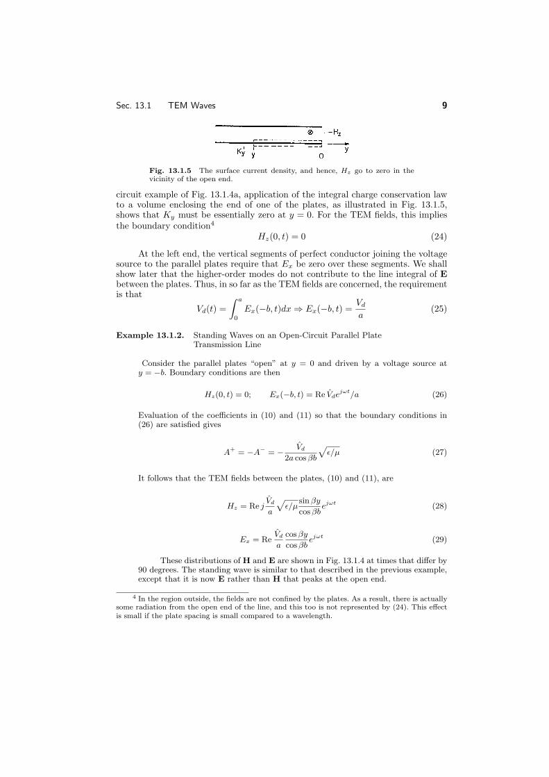
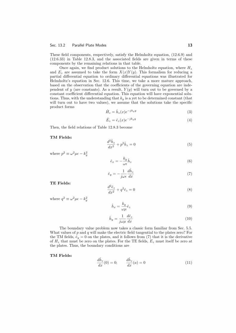
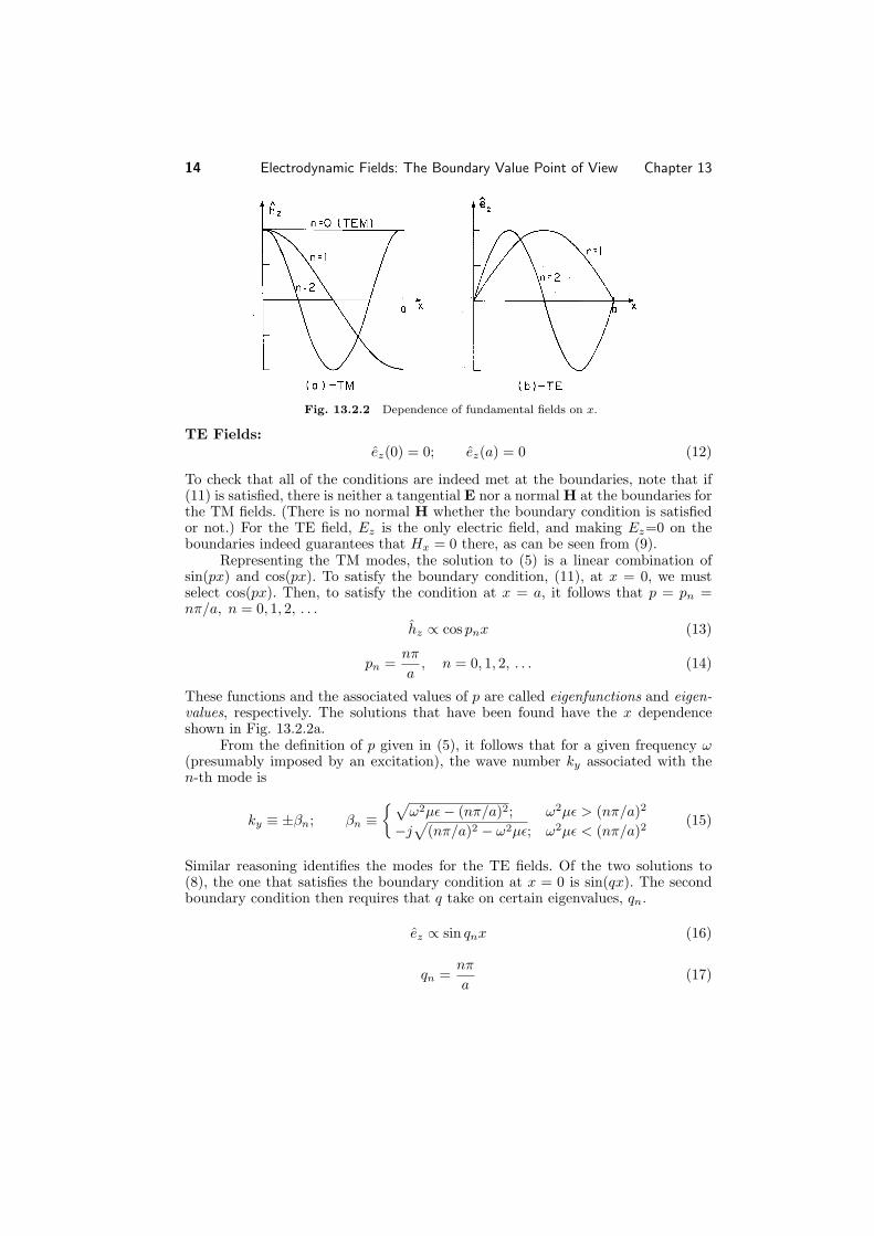
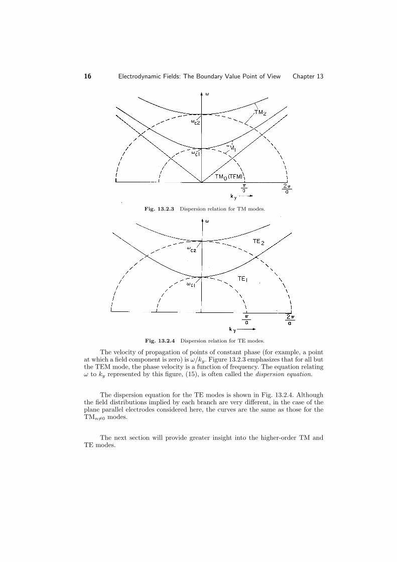
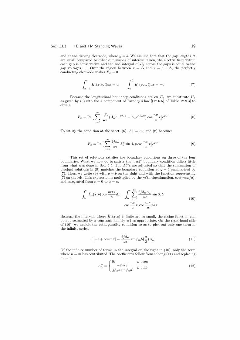
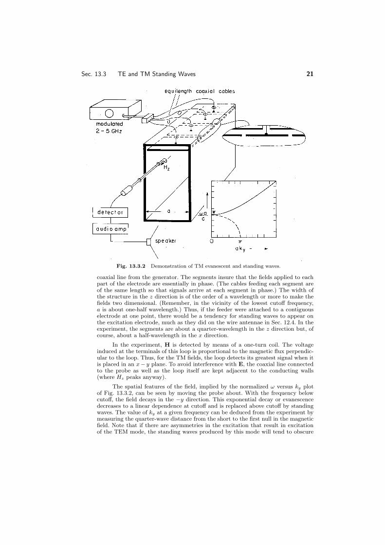

Cite as Markus Zahn course materials for 6641 Electromagnetic Fields Forces and Motion Spring 2005 MIT OpenCourseWare (httpocwmitedu) Massachusetts Institute of Technology Downloaded on [DD Month YYYY]
22 Electrodynamic Fields The Boundary Value Point of View Chapter 13
the TM1 mode when it is evanescent The TEM waves do not have a cutoff
As we have seen once again the TM fields are the electrodynamic generalizashytion of twoshydimensional EQS fields That is in the quasistatic limit the previous example becomes the capacitive attenuator of Sec 557
We have more than one reason to expect that the twoshydimensional TE fields are the generalization of MQS systems First this was seen to be the case in Sec 126 where the TE fields associated with a given surface current density were found to approach the MQS limit as ω2micro k2 Second from Sec 86 we know ythat for every twoshydimensional EQS configuration involving perfectly conducting boundaries there is an MQS one as well8 In particular the MQS analog of the capacitor attenuator is the configuration shown in Fig 1333 The MQS H field was found in Example 863
In treating MQS fields in the presence of perfect conductors we recognized that the condition of zero tangential E implied that there be no timeshyvarying normal B This made it possible to determine H without regard for E We could then delay taking detailed account of E until Sec 101 Thus in the MQS limit a system involving essentially a twoshydimensional distribution of H can (and usually does) have an E that depends on the third dimension For example in the configuration of Fig 1333 a voltage source might be used to drive the current in the z direction through the upper electrode This current is returned in the perfectly conducting shyshaped walls The electric fields in the vicinities of the gaps must therefore increase in the z direction from zero at the shorts to values consistent with the voltage sources at the near end Over most of the length of the system E is across the gap and therefore in planes perpendicular to the z axis This MQS configuration does not excite pure TE fields In order to produce (approximately) twoshydimensional TE fields provision must be made to make E as well as H two dimensional The following example and demonstration give the opportunity to further develop an appreciation for TE fields
Example 1332 Excitation of TE Modes and the MQS Limit
An idealized configuration for exciting standing TE modes is shown in Fig 1334 As in Example 1331 the perfectly conducting plates are shorted in the plane y = 0 In the plane y = b is a perfectly conducting plate that is segmented in the z direction Each segment is driven by a voltage source that is itself distributed in the x direction In the limit where there are many of these voltage sources and perfectly conducting segments the driving electrode becomes one that both imposes a zshydirected E and has no z component of B That is just below the surface of this electrode wEz is equal to the sum of the source voltages One way of approximately realizing this idealization is used in the next demonstration
Let Λ be defined as the flux per unit length (length taken along the z direction) into and out of the enclosed region through the gaps of width Δ between the driving electrode and the adjacent edges of the plane parallel electrodes The magnetic field
7 The example which was the theme of Sec 55 might equally well have been called the ldquomicrowave attenuatorrdquo for a section of waveguide operated below cutoff is used in microwave circuits to attenuate signals
8 The H satisfying the condition that n B = 0 on the perfectly conducting boundaries was middot obtained by replacing Φ Az in the solution to the analogous EQS problem rarr
Cite as Markus Zahn course materials for 6641 Electromagnetic Fields Forces and Motion Spring 2005 MIT OpenCourseWare (httpocwmitedu) Massachusetts Institute of Technology Downloaded on [DD Month YYYY]
Sec 133 TE and TM Standing Waves 23
Fig 1333 Twoshydimensional MQS configuration that does not have TEfields
Fig 1334 Idealized configuration for excitation of TE standing waves
normal to the driving electrode between the gaps is zero Thus at the upper surface Hy has the distribution shown in Fig 1335a
Faradayrsquos integral law applied to the contour C of Fig 1334 and to a similar contour around the other gap shows that
Ez(x b t) = minus d
dt
Λ rArr E z = minusjωΛ (16)
24 Electrodynamic Fields The Boundary Value Point of View Chapter 13
Fig 1335 Equivalent boundary conditions on normal H and tanshygential E at y = b
Thus either the normal B or the tangential E on the surface at y = b is specified The two must be consistent with each other ie they must obey Faradayrsquos law It is perhaps easiest in this case to deal directly with Ez in finding the coefficients apshypearing in (13220) Once they have been determined (much as in Example 1331) H follows from Faradayrsquos law (12629) and (12630) of Table 1283
infin 4jΛω sin βmy mπx jωtEz = Re sin e (17)
minus
mπ sin βmb a m=1 odd
infin 4βmΛ cos βmy mπx jωt Hx = Re
sin e (18)
micromπ sin βmb a m=1 odd
infin Λ sin βmy mπx jωt Hy = Re
minus4ˆcos e (19)
microa sin βmb a m=1 odd
In the quasistatic limit ω2micro (mπa)2 this magnetic field reduces to that found in Example 863
A few observations may help one to gain some insights from these expressions First if the magnetic field is sensed then the detection loop must have its axis in the xminus y plane For these TE modes there should be no signal sensed with the axis of the detection loop in the z direction This probe can also be used to verify that H normal to the perfectly conducting surfaces is indeed zero while its tangential value peaks at the short Second the same decay of the fields below cutoff and appearance of standing waves above cutoff is predicted here as in the TM case Third because E is perpendicular to planes of constant z the boundary conditions on E and hence H are met even if perfectly conducting plates are placed over the open ends of the guide say in the planes z = 0 and z = w In this case the guide becomes a closed pipe of rectangular crossshysection What we have found are then a subset of the threeshydimensional modes of propagation in a rectangular waveguide
Demonstration 1332 Evanescent and Standing TE Waves
The apparatus of Demonstration 1331 is altered to give TE rather than TM waves by using an array of ldquooneshyturn inductorsrdquo rather than the array of ldquocapacitor platesrdquo These are shown in Fig 1336
Sec 134 Rectangular Waveguide Modes 25
Fig 1336 Demonstration of evanescent and standing TE waves
Each member of the array consists of an electrode of width a minus 2Δ driven at one edge by a common source and shorted to the perfectly conducting backing at its other edge Thus the magnetic flux through the closed loop passes into and out of the guide through the gaps of width Δ between the ends of the oneshyturn coil and the parallel plate (vertical) walls of the guide Effectively the integral of Ez created by the voltage sources in the idealized model of Fig 1334 is produced by the integral of Ez between the left edge of one current loop and the right edge of the next
The current loop can be held in the x minus z plane to sense Hy or in the y minus z plane to sense Hx to verify the field distributions derived in the previous example It can also be observed that placing conducting sheets against the open ends of the parallel plate guide making it a rectangular pipe guide leaves the characteristics of these twoshydimensional TE modes unchanged
134 RECTANGULAR WAVEGUIDE MODES
Metal pipe waveguides are often used to guide electromagnetic waves The most common waveguides have rectangular crossshysections and so are well suited for the exploration of electrodynamic fields that depend on three dimensions Although we confine ourselves to a rectangular crossshysection and hence Cartesian coordinates the classification of waveguide modes and the general approach used here are equally applicable to other geometries for example to waveguides of circular crossshysection
The parallel plate system considered in the previous three sections illustrates
Cite as Markus Zahn course materials for 6641 Electromagnetic Fields Forces and Motion Spring 2005 MIT OpenCourseWare (httpocwmitedu) Massachusetts Institute of Technology Downloaded on [DD Month YYYY]
26 Electrodynamic Fields The Boundary Value Point of View Chapter 13
Fig 1341 Rectangular waveguide
much of what can be expected in pipe waveguides However unlike the parallel plates which can support TEM modes as well as highershyorder TE modes and TM modes the pipe cannot transmit a TEM mode From the parallel plate system we expect that a waveguide will support propagating modes only if the frequency is high enough to make the greater interior crossshysectional dimension of the pipe greater than a free space halfshywavelength Thus we will find that a guide having a larger dimension greater than 5 cm would typically be used to guide energy having a frequency of 3 GHz
We found it convenient to classify twoshydimensional fields as transverse magshynetic (TM) or transverse electric (TE) according to whether E or H was transshyverse to the direction of propagation (or decay) Here where we deal with threeshydimensional fields it will be convenient to classify fields according to whether they have E or H transverse to the axial direction of the guide This classification is used regardless of the crossshysectional geometry of the pipe We choose again the y coordinate as the axis of the guide as shown in Fig 1341 If we focus on solutions to Maxwellrsquos equations taking the form
Hy = Re hy(x z)ej(ωtminuskyy) (1)
Ey = Re ey(x z)ej(ωtminuskyy) (2)
then all of the other complex amplitude field components can be written in terms of the complex amplitudes of these axial fields Hy and Ey This can be seen from substituting fields having the form of (1) and (2) into the transverse components of Amperersquos law (1208)
minusjkyhz minus parth
y = jωex (3)partz
Sec 134 Rectangular Waveguide Modes 27
parth y + jkyh
x = jωez (4)partx
and into the transverse components of Faradayrsquos law (1209)
minusjky ez minus partey = minusjωmicrohx (5)partz
partey + jky ex = minusjωmicrohz (6)partx
If we take h y and ˆ ey as specified (3) and (6) constitute two algebraic equations in
the unknowns ˆ ex and h z Thus they can be solved for these components Similarly
h x and ez follow from (4) and (5)
parth
y partey
h
x = minus jky partx
minus jω (ω2micro minus k2) (7)partz y
h z =
minus jky parth
y + jω partey
(ω2micro minus k2) (8)
partz partx y
ex =
jωmicro parth
y minus jky partey
(ω2micro minus ky
2) (9)partz partx
parthy partˆ ez =
minus jωmicropartx
minus jky ey
(ω2micro minus ky
2) (10)partz
We have found that the threeshydimensional fields are a superposition of those associated with Ey (so that the magnetic field is transverse to the guide axis ) the TM fields and those due to Hy the TE modes The axial field components now play the role of ldquopotentialsrdquo from which the other field components can be derived
We can use the y components of the laws of Ampere and Faraday together with Gaussrsquo law and the divergence law for H to show that the axial complex amplitudes ˆ ey and h
y satisfy the twoshydimensional Helmholtz equations
TM Modes (Hy = 0)
part2ey
partx2 +
part2ey
partz2 + p 2 ey = 0 (11)
where 2 p = ω2micro minus k2
y
and
TE Modes (Ey = 0)
part2hy part2h y+ + q 2h
y = 0 (12)partx2 partz2
28 Electrodynamic Fields The Boundary Value Point of View Chapter 13
where q 2 = ω2micro minus ky
2
These relations also follow from substitution of (1) and (2) into the y components of (1302) and (1301)
The solutions to (11) and (12) must satisfy boundary conditions on the pershyfectly conducting walls Because Ey is parallel to the perfectly conducting walls it must be zero there
TM Modes
ey(0 z) = 0 ey(a z) = 0 ey(x 0) = 0 ey(xw) = 0 (13)
The boundary condition on Hy follows from (9) and (10) which express ex
and ˆ ez in terms of h y On the walls at x = 0 and x = a ez = 0 On the walls at
z = 0 z = w ex = 0 Therefore from (9) and (10) we obtain
TE Modes
parthy (0 z) = 0 parthy (a z) = 0
parthy (x 0) = 0 parthy (x w) = 0 (14)
partx partx partz partz
The derivative of hy with respect to a coordinate perpendicular to the boundary must be zero
The solution to the Helmholtz equation (11) or (12) follows a pattern that is familiar from that used for Laplacersquos equation in Sec 54 Either of the complex amplitudes representing the axial fields is represented by a product solution
ey
ˆ prop X(x)Z(z) (15)hy
Substitution into (11) or (12) and separation of variables then gives
d2X + γ2X = 0 (16)
dx2
d2Z + δ2Z = 0
dz2
where
minusγ2 minus δ2 +
p2
2
= 0 (17)q
Solutions that satisfy the TM boundary conditions (13) are then
TM Modes
mπ X prop sin γmx γm = m = 1 2 (18)
a
29 Sec 134 Rectangular Waveguide Modes
nπ Z prop sin δnz δn = n = 1 2
w
so that pmn 2 =
mπ 2 + nπ 2 m = 1 2 n = 1 2 (19)
a w
When either m or n is zero the field is zero and thus m and n must be equal to an integer equal to or greater than one For a given frequency ω and mode number (mn) the wave number ky is found by using (19) in the definition of p associated with (11)
ky = plusmnβmn
with ⎧ ω2micro minus
mπ
2 minus
nπ 2 2 +
nπ
2⎨ w ω2micro gt
mπ
w (20)βmna a equiv ⎩ minusj
mπ
2 +
nπ 2 minus ω2micro ω2micro lt
mπ
2 +
nπ 2
a w a w
Thus the TM solutions are
infin infin mπ nπ
Ey = Re
(A+ eminusjβmn y + Aminus ejβmn y) sin x sin z ejωt (21)mn mn a w m=1 n=1
For the TE modes (14) provides the boundary conditions and we are led to the solutions
TE Modes
mπ X prop cos γmx γm = m = 0 1 2 (22)
a
nπ Z prop cos δnz δn = n = 0 1 2
a
Substitution of γm and δn into (17) therefore gives
q 2 = mπ 2 +
nπ 2 m = 0 1 2 n = 0 1 2 (23)mn a w
(mn) = (0 0)
The wave number ky is obtained using this eigenvalue in the definition of q assoshyciated with (12) With the understanding that either m or n can now be zero the expression is the same as that for the TM modes (20) However both m and n cannot be zero If they were it follows from (22) that the axial H would be uniform over any given crossshysection of the guide The integral of Faradayrsquos law over the crossshysection of the guide with the enclosing contour C adjacent to the perfectly conducting boundaries as shown in Fig 1342 requires that
E ds = minusmicroA
dHy (24)middot dt
30 Electrodynamic Fields The Boundary Value Point of View Chapter 13
Fig 1342 Crossshysection of guide with contour adjacent to perfectly conshyducting walls
where A is the crossshysectional area of the guide Because the contour on the left is adjacent to the perfectly conducting boundaries the line integral of E must be zero It follows that for the m = 0 n = 0 mode Hy = 0 If there were such a mode it would have both E and H transverse to the guide axis We will show in Sec 142 where TEM modes are considered in general that TEM modes cannot exist within a perfectly conducting pipe
Even though the dispersion equations for the TM and TE modes only differ in the allowed lowest values of (mn) the field distributions of these modes are very different9 The superposition of TE modes gives
infin infin mπ nπ
Re
(C+ eminusjβmn y + Cminus jβmn y) jωt Hy = mn mne cos x cos z e (25) a w
middot m=0 n=0
where m n = 0 The frequency at which a given mode switches from evanescence middot to propagation is an important parameter This cutoff frequency follows from (20) as
1 mπ 2 +
nπ 2 ωc = radic
micro a w (26)
TM Modes m = 0 n = 0
TE Modes m and n not both zero
Rearranging this expression gives the normalized cutoff frequency as functions of the aspect ratio aw of the guide
ωcw ωc equiv
cπ =
(wa)2m2 + n2 (27)
These normalized cutoff frequencies are shown as functions of wa in Fig 1343 The numbering of the modes is standardized The dimension w is chosen as
w le a and the first index m gives the variation of the field along a The TE10
9 In other geometries such as a circular waveguide this coincidence of pmn and qmn is not found
Sec 134 Rectangular Waveguide Modes 31
Fig 1343 Normalized cutoff frequencies for lowest rectangular waveguide modes as a function of aspect ratio
mode then has the lowest cutoff frequency and is called the dominant mode All other modes have higher cutoff frequencies (except of course in the case of the square crossshysection for which TE01 has the same cutoff frequency) Guides are usually designed so that at the frequency of operation only the dominant mode is propagating while all highershyorder modes are ldquocutoffrdquo
In general an excitation of the guide at a crossshysection y = constant excites all waveguide modes The modes with cutoff frequencies higher than the frequency of excitation decay away from the source Only the dominant mode has a sinusoidal dependence upon y and thus possesses fields that are periodic in y and ldquodominaterdquo the field pattern far away from the source at distances larger than the transverse dimensions of the waveguide
Example 1341 TE10 Standing Wave Fields
The section of rectangular guide shown in Fig 1344 is excited somewhere to the right of y = 0 and shorted by a conducting plate in the plane y = 0 We presume that the frequency is above the cutoff frequency for the TE10 mode and that a gt w as shown The frequency of excitation is chosen to be below the cutoff frequency for all higher order modes and the source is far away from y = 0 (ie at y a) The field in the guide is then that of the TE10 mode Thus Hy is given by (25) with m = 1 and n = 0 What is the spaceshytime dependence of the standing waves that result from having shorted the guide
Because of the short Ez(x y = 0 z) = 0 In order to relate the coefficients
C+ and Cminus we must determine ˆ ez from h y as given by (25) using (10) 10 10
a 10e
minusjβ10y jβ10y πx jωt 10eEz = Re jωmicro (C+ + Cminus ) sin e (28)
π a
and because ez = 0 at the short it follows that
C+ = minusCminus (29)10 10
32 Electrodynamic Fields The Boundary Value Point of View Chapter 13
Fig 1344 Fields and surface sources for TE10 mode
so that a π jωt
Ez = 2ωmicro C+ xe (30)Re 10 sin β10y sin
π a
and this is the only component of the electric field in this mode We can now use (29) to evaluate (25)
π jωt
Hy = minusRe 2jC+ cos xe (31)10 sin β10y
a
In using (7) to evaluate the other component of H remember that in the C+ termmn
of (25) ky = βmn while in the Cminus term ky = minusβmnmn
a π jωt
C+Hx = Re 2jβ10 10 cos β10y sin xe (32)
π a
To sketch these fields in the neighborhood of the short and deduce the associshyated surface charge and current densities consider C+ to be real The j in (31) and 10
(32) shows that Hx and Hy are 90 degrees out of phase with the electric field Thus in the field sketches of Fig 1344 E and H are shown at different instants of time say E when ωt = π and H when ωt = π2 The surface charge density is where Ez
terminates and originates on the upper and lower walls The surface current density can be inferred from Amperersquos continuity condition The temporal oscillations of these fields should be pictured with H equal to zero when E peaks and with E equal to zero when H peaks At planes spaced by multiples of a halfshywavelength along the y axis E is always zero
Sec 135 Optical Fibers 33
Fig 1345 Slotted line for measuring axial distribution of TE10 fields
The following demonstration illustrates how a movable probe designed to coushyple to the electric field is introduced into a waveguide with minimal disturbance of the wall currents
Demonstration 1341 Probing the TE10 Mode
A waveguide slotted line is shown in Fig 1345 Here the line is shorted at y = 0 and excited at the right The probe used to excite the guide is of the capacitive type positioned so that charges induced on its tip couple to the lines of electric field shown in Fig 1344 This electrical coupling is an alternative to the magnetic coupling used for the TE mode in Demonstration 1332
The y dependence of the field pattern is detected in the apparatus shown in Fig 1345 by means of a second capacitive electrode introduced through a slot so that it can be moved in the y direction and not perturb the field ie the wall is cut along the lines of the surface current K From the sketch of K given in Fig 1344 it can be seen that K is in the y direction along the center line of the guide
The probe can be used to measure the wavelength 2πky of the standing waves by measuring the distance between nulls in the output signal (between nulls in Ez) With the frequency somewhat below the cutoff of the TE10 mode the spatial decay away from the source of the evanescent wave also can be detected
135 DIELECTRIC WAVEGUIDES OPTICAL FIBERS
Waves can be guided by dielectric rods or slabs and the fields of these waves occupy the space within and around these dielectric structures Especially at optical wavelengths dielectric fibers are commonly used to guide waves In this section we develop the properties of waves guided by a planar sheet of dielectric material The waves that we find are typical of those found in integrated optical systems and in the more commonly used optical fibers of circular crossshysection
A planar version of a dielectric waveguide is pictured in Fig 1351 A dielectric of thickness 2d and permittivity i is surrounded by a dielectric of permittivity lt i The latter might be free space with = o We are interested in how this
34 Electrodynamic Fields The Boundary Value Point of View Chapter 13
Fig 1351 Dielectric slab waveguide
structure might be used to guide waves in the y direction and will confine ourselves to fields that are independent of z
With a source somewhere to the left (for example an antenna imbedded in the dielectric) there is reason to expect that there are fields outside as well as inside the dielectric We shall look for field solutions that propagate in the y direction and possess fields solely inside and near the layer The fields external to the layer decay to zero in the plusmnx directions Like the waves propagating along waveguides those guided by this structure have transverse components that take the form
Ez = Re ˆ ez(x)ej(ωtminuskyy) (1)
both inside and outside the dielectric That is the fields inside and outside the dielectric have the same frequency ω the same phase velocity ωky and hence the same wavelength 2πky in the y direction Of course whether such fields can actually exist will be determined by the following analysis
The classification of twoshydimensional fields introduced in Sec 126 is applicashyble here The TM and TE fields can be made to independently satisfy the boundary conditions so that the resulting modes can be classified as TM or TE10 Here we will confine ourselves to the transverse electric modes In the exterior and interior regions where the permittivities are uniform but different it follows from substishytution of (1) into (12633) (Table 1283) that
d2ez minus α2 xez = 0 αx =
ky
2 minus ω2micro d lt x and x lt minusd (2)dx2
d2ez + k2 ez = 0 kx =
ω2microi minus k2 minusd lt x lt d (3)dx2 x y
A guided wave is one that is composed of a nonuniform plane wave in the exterior regions decaying in the plusmnx directions and propagating with the phase velocity ωky in the y direction In anticipation of this we have written (2) in
10 Circular dielectric rods do not support simple TE or TM waves in that case this classifishycation of modes is not possible
Sec 135 Optical Fibers 35
terms of the parameter αx which must then be real and positive Through the continuity conditions the exterior wave must match up to the interior wave at the dielectric surfaces The solutions to (3) are sines and cosines if kx is real In order to match the interior fields onto the nonuniform plane waves on both sides of the guide it is necessary that kx be real
We now set out to find the wave numbers ky that not only satisfy the wave equations in each of the regions represented by (2) and (3) but the continuity conditions at the interfaces as well The configuration is symmetric about the x = 0 plane so we can further divide the modes into those that have even and odd functions Ez(x) Thus with A an arbitrary factor appropriate even solutions to (2) and (3) are ⎧
⎪⎪⎨
⎪⎪⎩
Aeminusαx(xminusd) d lt x cos kxx
ez = A minusd lt x lt d (4)cos kxd
Aeαx(x+d) x lt minusd
To simplify the algebra we have displaced the origin in the exterior solutions so that just the coefficient A is obtained when ez is evaluated at the respective interfaces With a similar objective the interior solution has been divided by the constant cos(kxd) so that at the boundaries ez also becomes A In this way we have adjusted the interior coefficient so that ez is continuous at the boundaries
Because this transverse field is the only component of E all of the continuity conditions on E are now satisfied The permeabilities of all regions are presumed to be the same so both tangential and normal components of H must be continuous at the boundaries From (12629) the continuity of normal microH is guaranteed by the continuity of Ez in any case The tangential field is obtained using (12630)
h y =
1 dez (5)jωmicro dx
Substitution of (4) into (5) gives
hy = 1
jωmicro
⎧⎨
⎩
minusα Aeminusαx(xminusd) d lt x minusk
x
A sin kxx minusd lt x lt d (6)cos kxdx
αxAeαx(x+d) x lt minusd
The assumption that Ez is even in x has as a consequence the fact that the continushyity condition on tangential H is satisfied by the same relation at both boundaries
αx minusαxA = minuskxA tan kxd rArr kx
= tan kxd (7)
Our goal is to determine the propagation constant ky for a given ω If we were to substitute the definitions of αx and kx into this expression we would have this dispersion equation D(ωky) implicitly relating ky to ω It is more convenient to solve for αx and kx first and then for ky
Elimination of ky between the expressions for αx and kx given with (2) and (3) gives a second expression for αxkx
αx =
ω2microid2
1minus minus 1 (8)
kx (kxd)2 i
36 Electrodynamic Fields The Boundary Value Point of View Chapter 13
Fig 1352 Graphical solution to (7) and (8)
The solutions for the values of the normalized transverse wave numbers (kxd) can be pictured as shown in Fig 1352 Plotted as functions of kxd are the rightshyhand sides of (7) and (8) The points of intersection kxd = γm are the desired solutions For the frequency used to make Fig 1352 there are two solutions These are designated by even integers because the odd modes (Prob 1351) have roots that interleave these even modes
As the frequency is raised an additional even TEshyguided mode is found each time the curve representing (8) reaches a new branch of (7) This happens at freshyquencies ωc such that αxkx = 0 and kxd = mπ2 where m = 0 2 4 From (8)
mπ 1 ωc = (9)
2d
micro(i minus )
The m = 0 mode has no cutoff frequency To finally determine ky from these eigenvalues the definition of kx given with
(3) is used to write kyd =
ω2microid2 minus (kxd)2 (10)
and the dispersion equation takes the graphical form of Fig 1353 To make Fig 1352 we had to specify the ratio of permittivities so that ratio is also implicit in Fig 1353
Features of the dispersion diagram Fig 1353 can be gathered rather simply Where a mode is just cutoff because ω = ωc αx = 0 as can be seen from Fig 1352 From (2) we gather that ky = ωc
radicmicro Thus at cutoff a mode must have a
propagation constant ky that lies on the straight broken line to the left shown in Fig 1353 At cutoff each mode has a phase velocity equal to that of a plane wave in the medium exterior to the layer
In the highshyfrequency limit where ω goes to infinity we see from Fig 1352 that kxd approaches the constant kx (m + 1)π2d That is in (3) kx becomes a rarrconstant even as ω goes to infinity and it follows that in this high frequency limit ky ω
radicmicroi rarr
Sec 135 Optical Fibers 37
Fig 1353 Dispersion equation for even TE modes with i = 66
Fig 1354 Distribution of transverse E for TE0 mode on dielectric wavegshyuide of Fig 1351
The physical reasons for this behavior follow from the nature of the mode pattern as a function of frequency When αx 0 as the frequency approaches rarrcutoff it follows from (4) that the fields extend far into the regions outside of the layer The wave approaches an infinite parallel plane wave having a propagation constant that is hardly affected by the layer In the opposite extreme where ω goes to infinity the decay of the external field is rapid and a given mode is well confined inside the layer Again the wave assumes the character of an infinite parallel plane wave but in this limit one that propagates with the phase velocity of a plane wave in a medium with the dielectric constant of the layer
The distribution of Ez of the m = 0 mode at one frequency is shown in Fig 1354 As the frequency is raised each mode becomes more confined to the layer
38 Electrodynamic Fields The Boundary Value Point of View Chapter 13
Fig 1355 Dielectric waveguide demonstration
Demonstration 1351 Microwave Dielectric Guided Waves
In the experiment shown in Fig 1355 a dielectric slab is demonstrated to guide microwaves To assure the excitation of only an m = 0 TEshyguided wave but one as well confined to the dielectric as possible the frequency is made just under the cutoff frequency ωc2 (For a 2 cm thick slab having io = 66 this is a frequency just under 6 GHz) The m = 0 wave is excited in the dielectric slab by means of a vertical element at its left edge This assures excitation of Ez while having the symmetry necessary to avoid excitation of the odd modes
The antenna is mounted at the center of a metal ground plane Thus without the slab the signal at the receiving antenna (which is oriented to be sensitive to Ez) is essentially the same in all directions perpendicular to the z axis With the slab a sharply increased signal in the vicinity of the right edge of the slab gives qualitative evidence of the wave guidance The receiving antenna can also be used to probe the field decay in the x direction and to see that this decay increases with frequency11
136 SUMMARY
There are two perspectives from which this chapter can be reviewed First it can be viewed as a sequence of specific examples that are useful for dealing with radio frequency microwave and optical systems Secs 131ndash133 are concerned with the propagation of energy along parallel plates first acting as a transmission line and then as a waveguide Practical systems to which the derived properties of the TEM and highershyorder modes are directly applicable are strip lines used at frequencies
11 To make the excitation independent of z a collinear array of inshyphase dipoles could be used for the excitation This is not necessary to demonstrate the qualitative features of the guide
Cite as Markus Zahn course materials for 6641 Electromagnetic Fields Forces and Motion Spring 2005 MIT OpenCourseWare (httpocwmitedu) Massachusetts Institute of Technology Downloaded on [DD Month YYYY]
Sec 136 Summary 39
that extend from dc to the microwave range The rectangular waveguide of Sec 134 might well be a section of ldquoplumbingrdquo from a microwave communication system and the dielectric waveguide of Sec 135 has many of the properties of an optical fiber Second the mathematical analysis of waves exemplified in this chapter is generally applicable to other more complex systems that are uniform in one direction
When the structures described in this chapter are used to transport energy from one location to another they are generally not terminated in ldquoshortsrdquo and ldquoopensrdquo and hence generally do not simply support standing waves The object is usually to carry energy from an antenna to a receiver or from a generator to a load whether that be an antenna or a light bulb Such energy transport is accomplished by the traveling waves featured in the next chapter
40 Electrodynamic Fields The Boundary Value Point of View Chapter 13
P R O B L E M S
131 Introduction to TEM Waves
1311lowast With a short at y = 0 it is possible to find the fields for Example 1311 by recognizing at the outset that standing wave solutions meeting the homogeshyneous boundary condition of (12) are of the form Ex = Re A sin(βy) exp(jωt)
(a) Use (1312) and (1313) to determine the associated Hz and the dispersion equation (relation between β and ω)
(b) Now use the boundary condition at y = minusb to show that the fields are as given by (13116) and (13117)
1312lowast Take the approach outlined in Prob 1311 for finding the fields [(13128) and (13129)] in Example 1312
1313 Assume that K o is real and express the standing wave of (13117) so as
to make it evident that it is the sum of equalshyamplitude waves traveling in the plusmny directions each with a magnitude of phase velocity ωβ = c and wavelength 2πβ
1314lowast Coaxial perfectly conducting circular cylinders having outer and inner radii a and b respectively form the transmission line shown in Fig P1314
(a) If the conductors were ldquoopen circuitrdquo at z = 0 and driven by a voltage source V at z = minusl show that the EQS electric field is radial and given by V[r ln(ab)]
(b) If the conductors were ldquoshortedrdquo at z = 0 and driven by a current source I at z = minusl show that the MQS magnetic field intensity is φ directed and given by I2πr
(c) With the motivation provided by these limiting solutions show that solutions to all of Maxwellrsquos equations (in the region between the conductors) that satisfy the boundary conditions on the surfaces of the coaxial conductors are
V (z t) I(z t)E = ir
ln
ab
r H = iφ 2πr
(a)
provided that V and I are now functions not only of t but of z as well that satisfy equations taking the same form as (1312) and (1313)
partI partV 2π
partz = minusC
partt C equiv
ln
a (b)
b
partV partI ln
ab
micro
partz = minusL
partt L equiv
2π (c)
Sec 132 Problems 41
Fig P1314
1315 For the coaxial configuration of Prob 1314 there is a perfectly conducting ldquoshortrdquo at z = 0 and the conductors are driven by a current source I = Re[Ioe
jωt] at z = minusl
(a) Find I(z t) and V (z t) and hence E and H (b) Take the low frequency limit where ω
radicmicrol 1 and show that E and
H are the same as for a coaxial inductor (c) Find E and H directly from the MQS laws and show that they agree
with the results of part (b)
1316 For the coaxial configuration of Prob 1314 the conductors are ldquoopen circuitedrdquo at z = 0 and driven by a voltage source V = Re [Vo exp(jωt] at x = minusl
(a) Find I(z t) and V (z t) and hence E and H (b) Take the lowshyfrequency limit where ω
radicmicrol 1 and show that E and
H are the same as for a coaxial capacitor (c) Find E and H directly from the EQS laws and show that they agree
with the results of (b)
132 TwoshyDimensional Modes Between Parallel Plates
1321lowast Show that each of the highershyorder modes propagating in the +y direcshytion represented by A+
n and Cn + in (13219) and (13220) respectively
can be regarded as the sum of plane waves propagating in the directions represented by the vector wave number
nπk = + βn (a)plusmn
a ix iy
and interfering in the planes x = 0 and x = a so as to satisfy the boundary conditions
1322 The TM and TE modes can themselves be classified into odd or even modes that respectively have h
z or ˆ ez odd or even functions of x With this in mind the origin of the coordinate system is moved so that it is midway between the perfectly conducting plates as shown in Fig P1322
42 Electrodynamic Fields The Boundary Value Point of View Chapter 13
Fig P1322
(a) Find the odd TM and TE solutions Note that when the boundary condition is met at x = d equiv a2 for these functions it is automatically met at x = minusd
(b) Find the even TM and TE solutions again noting that if the condishytions are met at x = d then they are at x = minusd as well
133 TE and TM Standing Waves between Parallel Plates
1331lowast Starting with (1331) (for TM modes) and (1332) (for TE modes) use steps similar to those illustrated by (5520)ndash(5526) to obtain the orthogshyonality conditions of (1333) and (1334) respectively
1332 In the system of Example 1331 the wall at y = 0 is replaced by that shown in Fig P1332 A strip electrode is embedded in but insulated from the wall at y = 0 The resistance R is low enough so that E tangential to the boundary at y = 0 even at the insulating gaps between the strip electrode and the surrounding wall is negligible
(a) Determine the output voltage vo in terms of v (b) For ba = 2 describe the dependence of vo on frequency over the | |
range ωradic
micro a = 0 π
54 specifying the lowshyfrequency range where the response
rarrhas a linear dependence on frequency and the
resonance frequencies (c) What is the distribution of Hz(x y) at the resonance frequencies
1333lowast In the twoshydimensional system of Fig P1333 each driven electrode has the same nature as the one in Fig 1331 The origin of the y axis has been chosen to be in the plane of symmetry
(a) Use the symmetry to argue that Hz(y = 0) = 0
Sec 133 Problems 43
Fig P1332
Fig P1333
(b) Show that in the interior region
infin minus4jωv sin βny nπx jωt Hz = Re
cos e (a)βna cos βnb a
n=1 odd
1334 The oneshyturn loop of Fig P1334 has dimensions that are small compared to a b or wavelengths of interest and has area A in the x minus y plane
(a) It is used to detect the TM H field at the middle of the bottom electrode in Fig 1331 Assume that the resistance is large enough so that the current induced in this loop gives rise to a magnetic field that is negligible compared to that already found In terms of Hz what is vo
(b) At what locations x = X of the loop is a maximum |vo|(c) If the same loop were in the plate at y = 0 in the configuration of Fig
1313 and used to detect Hz at y = 0 for the TEM fields of Example
44 Electrodynamic Fields The Boundary Value Point of View Chapter 13
Fig P1334
1311 what would be the dependence of vo on the location x = X of the loop
| |
(d) If the loop were located in the plate at y = 0 in the TE configuration of Fig 1334 how should the loop be oriented to detect H
1335 In the system shown in Fig P1335 Δ d and the driving sources v = Re[v exp(jωt)] are uniformly distributed in the z direction so that the fields are two dimensional Thus the driving electrode is like that of Fig 1331 except that it spans the width d rather than the full width a Find H and E in terms of v
1336 In the system shown in Fig P1336 the excitation electrode is like that for Fig 1334 except that it has a width d rather than a Find H and E in terms of Λ
134 Rectangular Waveguide Modes
1341lowast Show that an alternative method of exciting and detecting the TE10 mode in Demonstration 1341 is to introduce oneshyturn loops as shown in Fig P1341 The excitation loop is inserted through a hole in the conducting wall while the detection loop passes through a slot so that it can be moved in the y direction The loops are each in the y minus z plane To minimize disturbance of the field the detection loop is terminated in a high enough impedance so that the field from the current in the loop is negligible Comshypare the y dependence of the detected signal to that measured using the electric probe
1342 A rectangular waveguide has wa = 075 Presuming that all TE and TM modes are excited in the guide in what order do the lowest six modes begin to propagate in the y direction as the frequency is raised
1343lowast The rectangular waveguide shown in Fig P1343 is terminated in a pershyfectly conducting plate at y = 0 that makes contact with the guide walls An electrode at y = b has a gap of width Δ a and Δ w around its
45 Sec 134 Problems
Fig P1335
Fig P1336
Fig P1341
edges Distributed around this gap are sources that constrain the field from the edges of the plate to the guide walls to v(t)Δ = Re(vΔ) exp(jωt)
(a) Argue that the fields should be TM and use the boundary condition
46 Electrodynamic Fields The Boundary Value Point of View Chapter 13
Fig P1343
at y = 0 to show that
infin infin mπ nπˆ
2A+Ey = mn cos βmny sin x sin z (a)
a w m=1 n=1
[Hint If (1349) and (13410) are used remember that ky = +βmn
for the A+ mn mode but ky = minusβmn for the Aminus mode ] mn
(b) Show that for m and n both odd A+ = 8ˆ v(ω2microminusβ2 )nmπ2βmn sin(kmnb)mn mnwhile for either m or n even A+ = 0mn
(c) Show that for these modes the resonance frequencies (normalized to 1radic
microa) are
ωradic
microa = π
m2 + a
n2 +
ap2 (b)
w b
where m n and p are integers m and n odd (d) Show that under quasistatic conditions the field which has been found
is consistent with that implied by the EQS potential given by (51010) and (51015)
1344 The rectangular waveguide shown in Fig P1343 is terminated in a pershyfectly conducting plate at y = 0 that makes contact with the guide walls However instead of the excitation electrode shown at y = b there is the perfectly conducting plate with a square hole cut in its center shown in Fig P1344 In this hole the pole faces of a magnetic circuit are flush with the plate and are used to excite fields within the guide Approximate the normal fields over the surface of the pole faces as
H
o for a lt x lt a+Δ and wminusΔ lt z lt w+Δ
Hy = 2 2 2 2 (a)w+ΔminusH
o for aminus2Δ lt x lt a
2 and wminus2Δ lt z lt 2
Sec 135 Problems 47
Fig P1344
where Ho is a complex constant (Note that if the magnetic circuit is driven by a one turn coil the terminal voltage v = jω(Δ22)microH
o) Determine Hy and hence E and H inside the guide
135 Dielectric Waveguides Optical Fibers
1351lowast For the dielectric slab waveguide of Fig 1351 consider the TE modes that have Ez an odd function of z
(a) Show that the dispersion relation between ω and ky is again found from (13510) but with (kxd) found by simultaneously solving (1358) and
αx = minus cot kxd (a)kx
(b) Sketch the graphical solution for kxd equiv γm (m odd) and show that the cutoff frequency is again given by (1359) but with m odd rather than even
(c) Show that these odd modes also have the asymptote of unity slope shown in Fig 1353
(d) Sketch the odd mode dispersion relation on that for the even modes (Fig 1353)
1352 For the dielectric slab waveguide shown in Fig 1351 i = 25 micro = microo and d = 1 cm In Hz what is the highest frequency that can be used to guide only one TE mode (Note the result of Prob 1351)
1353lowast The dielectric slab waveguide of Fig 1351 is the same as that considered in this problem except that it now has a permeability microi that differs from that outside where it is micro
(a) Show that (1357) and (1358) respectively are replaced by
αx = micro
tan kxd
even (a)
kx microi minus cot kxd odd
48 Electrodynamic Fields The Boundary Value Point of View Chapter 13
αx =
ω2microiid2
1minus micro minus 1
kx (kxd)2 microii (b)
(b) Show that making microi gt micro lowers the cutoff frequency (c) For a given frequency does making microimicro gt 1 increase or decrease the
wavelength λ equiv 2πky
1354 The dielectric slab of Fig 1351 has permittivity i and permeability microi while in the surrounding regions these are and micro respectively Consider the TM modes
(a) Determine expressions analogous to (1357) (1358) and (13510) that can be used to determine the dispersion relation ω = ω(ky) for modes that have Hz even and odd functions of x
(b) What are the cutoff frequencies (c) For microi = micro and i = = 25 draw the dispersion plot for the lowest
three modes that is analogous to that of Fig 1353
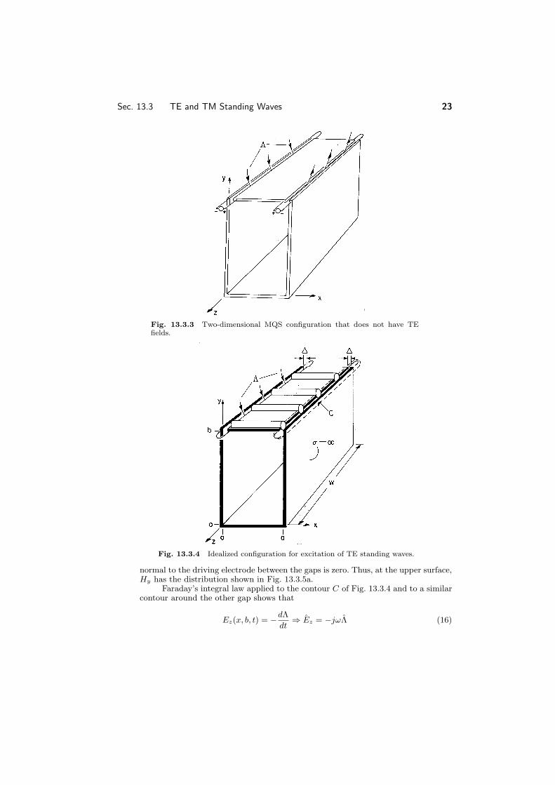
Cite as Markus Zahn course materials for 6641 Electromagnetic Fields Forces and Motion Spring 2005 MIT OpenCourseWare (httpocwmitedu) Massachusetts Institute of Technology Downloaded on [DD Month YYYY]
Sec 133 TE and TM Standing Waves 23
Fig 1333 Twoshydimensional MQS configuration that does not have TEfields
Fig 1334 Idealized configuration for excitation of TE standing waves
normal to the driving electrode between the gaps is zero Thus at the upper surface Hy has the distribution shown in Fig 1335a
Faradayrsquos integral law applied to the contour C of Fig 1334 and to a similar contour around the other gap shows that
Ez(x b t) = minus d
dt
Λ rArr E z = minusjωΛ (16)
24 Electrodynamic Fields The Boundary Value Point of View Chapter 13
Fig 1335 Equivalent boundary conditions on normal H and tanshygential E at y = b
Thus either the normal B or the tangential E on the surface at y = b is specified The two must be consistent with each other ie they must obey Faradayrsquos law It is perhaps easiest in this case to deal directly with Ez in finding the coefficients apshypearing in (13220) Once they have been determined (much as in Example 1331) H follows from Faradayrsquos law (12629) and (12630) of Table 1283
infin 4jΛω sin βmy mπx jωtEz = Re sin e (17)
minus
mπ sin βmb a m=1 odd
infin 4βmΛ cos βmy mπx jωt Hx = Re
sin e (18)
micromπ sin βmb a m=1 odd
infin Λ sin βmy mπx jωt Hy = Re
minus4ˆcos e (19)
microa sin βmb a m=1 odd
In the quasistatic limit ω2micro (mπa)2 this magnetic field reduces to that found in Example 863
A few observations may help one to gain some insights from these expressions First if the magnetic field is sensed then the detection loop must have its axis in the xminus y plane For these TE modes there should be no signal sensed with the axis of the detection loop in the z direction This probe can also be used to verify that H normal to the perfectly conducting surfaces is indeed zero while its tangential value peaks at the short Second the same decay of the fields below cutoff and appearance of standing waves above cutoff is predicted here as in the TM case Third because E is perpendicular to planes of constant z the boundary conditions on E and hence H are met even if perfectly conducting plates are placed over the open ends of the guide say in the planes z = 0 and z = w In this case the guide becomes a closed pipe of rectangular crossshysection What we have found are then a subset of the threeshydimensional modes of propagation in a rectangular waveguide
Demonstration 1332 Evanescent and Standing TE Waves
The apparatus of Demonstration 1331 is altered to give TE rather than TM waves by using an array of ldquooneshyturn inductorsrdquo rather than the array of ldquocapacitor platesrdquo These are shown in Fig 1336
Sec 134 Rectangular Waveguide Modes 25
Fig 1336 Demonstration of evanescent and standing TE waves
Each member of the array consists of an electrode of width a minus 2Δ driven at one edge by a common source and shorted to the perfectly conducting backing at its other edge Thus the magnetic flux through the closed loop passes into and out of the guide through the gaps of width Δ between the ends of the oneshyturn coil and the parallel plate (vertical) walls of the guide Effectively the integral of Ez created by the voltage sources in the idealized model of Fig 1334 is produced by the integral of Ez between the left edge of one current loop and the right edge of the next
The current loop can be held in the x minus z plane to sense Hy or in the y minus z plane to sense Hx to verify the field distributions derived in the previous example It can also be observed that placing conducting sheets against the open ends of the parallel plate guide making it a rectangular pipe guide leaves the characteristics of these twoshydimensional TE modes unchanged
134 RECTANGULAR WAVEGUIDE MODES
Metal pipe waveguides are often used to guide electromagnetic waves The most common waveguides have rectangular crossshysections and so are well suited for the exploration of electrodynamic fields that depend on three dimensions Although we confine ourselves to a rectangular crossshysection and hence Cartesian coordinates the classification of waveguide modes and the general approach used here are equally applicable to other geometries for example to waveguides of circular crossshysection
The parallel plate system considered in the previous three sections illustrates
Cite as Markus Zahn course materials for 6641 Electromagnetic Fields Forces and Motion Spring 2005 MIT OpenCourseWare (httpocwmitedu) Massachusetts Institute of Technology Downloaded on [DD Month YYYY]
26 Electrodynamic Fields The Boundary Value Point of View Chapter 13
Fig 1341 Rectangular waveguide
much of what can be expected in pipe waveguides However unlike the parallel plates which can support TEM modes as well as highershyorder TE modes and TM modes the pipe cannot transmit a TEM mode From the parallel plate system we expect that a waveguide will support propagating modes only if the frequency is high enough to make the greater interior crossshysectional dimension of the pipe greater than a free space halfshywavelength Thus we will find that a guide having a larger dimension greater than 5 cm would typically be used to guide energy having a frequency of 3 GHz
We found it convenient to classify twoshydimensional fields as transverse magshynetic (TM) or transverse electric (TE) according to whether E or H was transshyverse to the direction of propagation (or decay) Here where we deal with threeshydimensional fields it will be convenient to classify fields according to whether they have E or H transverse to the axial direction of the guide This classification is used regardless of the crossshysectional geometry of the pipe We choose again the y coordinate as the axis of the guide as shown in Fig 1341 If we focus on solutions to Maxwellrsquos equations taking the form
Hy = Re hy(x z)ej(ωtminuskyy) (1)
Ey = Re ey(x z)ej(ωtminuskyy) (2)
then all of the other complex amplitude field components can be written in terms of the complex amplitudes of these axial fields Hy and Ey This can be seen from substituting fields having the form of (1) and (2) into the transverse components of Amperersquos law (1208)
minusjkyhz minus parth
y = jωex (3)partz
Sec 134 Rectangular Waveguide Modes 27
parth y + jkyh
x = jωez (4)partx
and into the transverse components of Faradayrsquos law (1209)
minusjky ez minus partey = minusjωmicrohx (5)partz
partey + jky ex = minusjωmicrohz (6)partx
If we take h y and ˆ ey as specified (3) and (6) constitute two algebraic equations in
the unknowns ˆ ex and h z Thus they can be solved for these components Similarly
h x and ez follow from (4) and (5)
parth
y partey
h
x = minus jky partx
minus jω (ω2micro minus k2) (7)partz y
h z =
minus jky parth
y + jω partey
(ω2micro minus k2) (8)
partz partx y
ex =
jωmicro parth
y minus jky partey
(ω2micro minus ky
2) (9)partz partx
parthy partˆ ez =
minus jωmicropartx
minus jky ey
(ω2micro minus ky
2) (10)partz
We have found that the threeshydimensional fields are a superposition of those associated with Ey (so that the magnetic field is transverse to the guide axis ) the TM fields and those due to Hy the TE modes The axial field components now play the role of ldquopotentialsrdquo from which the other field components can be derived
We can use the y components of the laws of Ampere and Faraday together with Gaussrsquo law and the divergence law for H to show that the axial complex amplitudes ˆ ey and h
y satisfy the twoshydimensional Helmholtz equations
TM Modes (Hy = 0)
part2ey
partx2 +
part2ey
partz2 + p 2 ey = 0 (11)
where 2 p = ω2micro minus k2
y
and
TE Modes (Ey = 0)
part2hy part2h y+ + q 2h
y = 0 (12)partx2 partz2
28 Electrodynamic Fields The Boundary Value Point of View Chapter 13
where q 2 = ω2micro minus ky
2
These relations also follow from substitution of (1) and (2) into the y components of (1302) and (1301)
The solutions to (11) and (12) must satisfy boundary conditions on the pershyfectly conducting walls Because Ey is parallel to the perfectly conducting walls it must be zero there
TM Modes
ey(0 z) = 0 ey(a z) = 0 ey(x 0) = 0 ey(xw) = 0 (13)
The boundary condition on Hy follows from (9) and (10) which express ex
and ˆ ez in terms of h y On the walls at x = 0 and x = a ez = 0 On the walls at
z = 0 z = w ex = 0 Therefore from (9) and (10) we obtain
TE Modes
parthy (0 z) = 0 parthy (a z) = 0
parthy (x 0) = 0 parthy (x w) = 0 (14)
partx partx partz partz
The derivative of hy with respect to a coordinate perpendicular to the boundary must be zero
The solution to the Helmholtz equation (11) or (12) follows a pattern that is familiar from that used for Laplacersquos equation in Sec 54 Either of the complex amplitudes representing the axial fields is represented by a product solution
ey
ˆ prop X(x)Z(z) (15)hy
Substitution into (11) or (12) and separation of variables then gives
d2X + γ2X = 0 (16)
dx2
d2Z + δ2Z = 0
dz2
where
minusγ2 minus δ2 +
p2
2
= 0 (17)q
Solutions that satisfy the TM boundary conditions (13) are then
TM Modes
mπ X prop sin γmx γm = m = 1 2 (18)
a
29 Sec 134 Rectangular Waveguide Modes
nπ Z prop sin δnz δn = n = 1 2
w
so that pmn 2 =
mπ 2 + nπ 2 m = 1 2 n = 1 2 (19)
a w
When either m or n is zero the field is zero and thus m and n must be equal to an integer equal to or greater than one For a given frequency ω and mode number (mn) the wave number ky is found by using (19) in the definition of p associated with (11)
ky = plusmnβmn
with ⎧ ω2micro minus
mπ
2 minus
nπ 2 2 +
nπ
2⎨ w ω2micro gt
mπ
w (20)βmna a equiv ⎩ minusj
mπ
2 +
nπ 2 minus ω2micro ω2micro lt
mπ
2 +
nπ 2
a w a w
Thus the TM solutions are
infin infin mπ nπ
Ey = Re
(A+ eminusjβmn y + Aminus ejβmn y) sin x sin z ejωt (21)mn mn a w m=1 n=1
For the TE modes (14) provides the boundary conditions and we are led to the solutions
TE Modes
mπ X prop cos γmx γm = m = 0 1 2 (22)
a
nπ Z prop cos δnz δn = n = 0 1 2
a
Substitution of γm and δn into (17) therefore gives
q 2 = mπ 2 +
nπ 2 m = 0 1 2 n = 0 1 2 (23)mn a w
(mn) = (0 0)
The wave number ky is obtained using this eigenvalue in the definition of q assoshyciated with (12) With the understanding that either m or n can now be zero the expression is the same as that for the TM modes (20) However both m and n cannot be zero If they were it follows from (22) that the axial H would be uniform over any given crossshysection of the guide The integral of Faradayrsquos law over the crossshysection of the guide with the enclosing contour C adjacent to the perfectly conducting boundaries as shown in Fig 1342 requires that
E ds = minusmicroA
dHy (24)middot dt
30 Electrodynamic Fields The Boundary Value Point of View Chapter 13
Fig 1342 Crossshysection of guide with contour adjacent to perfectly conshyducting walls
where A is the crossshysectional area of the guide Because the contour on the left is adjacent to the perfectly conducting boundaries the line integral of E must be zero It follows that for the m = 0 n = 0 mode Hy = 0 If there were such a mode it would have both E and H transverse to the guide axis We will show in Sec 142 where TEM modes are considered in general that TEM modes cannot exist within a perfectly conducting pipe
Even though the dispersion equations for the TM and TE modes only differ in the allowed lowest values of (mn) the field distributions of these modes are very different9 The superposition of TE modes gives
infin infin mπ nπ
Re
(C+ eminusjβmn y + Cminus jβmn y) jωt Hy = mn mne cos x cos z e (25) a w
middot m=0 n=0
where m n = 0 The frequency at which a given mode switches from evanescence middot to propagation is an important parameter This cutoff frequency follows from (20) as
1 mπ 2 +
nπ 2 ωc = radic
micro a w (26)
TM Modes m = 0 n = 0
TE Modes m and n not both zero
Rearranging this expression gives the normalized cutoff frequency as functions of the aspect ratio aw of the guide
ωcw ωc equiv
cπ =
(wa)2m2 + n2 (27)
These normalized cutoff frequencies are shown as functions of wa in Fig 1343 The numbering of the modes is standardized The dimension w is chosen as
w le a and the first index m gives the variation of the field along a The TE10
9 In other geometries such as a circular waveguide this coincidence of pmn and qmn is not found
Sec 134 Rectangular Waveguide Modes 31
Fig 1343 Normalized cutoff frequencies for lowest rectangular waveguide modes as a function of aspect ratio
mode then has the lowest cutoff frequency and is called the dominant mode All other modes have higher cutoff frequencies (except of course in the case of the square crossshysection for which TE01 has the same cutoff frequency) Guides are usually designed so that at the frequency of operation only the dominant mode is propagating while all highershyorder modes are ldquocutoffrdquo
In general an excitation of the guide at a crossshysection y = constant excites all waveguide modes The modes with cutoff frequencies higher than the frequency of excitation decay away from the source Only the dominant mode has a sinusoidal dependence upon y and thus possesses fields that are periodic in y and ldquodominaterdquo the field pattern far away from the source at distances larger than the transverse dimensions of the waveguide
Example 1341 TE10 Standing Wave Fields
The section of rectangular guide shown in Fig 1344 is excited somewhere to the right of y = 0 and shorted by a conducting plate in the plane y = 0 We presume that the frequency is above the cutoff frequency for the TE10 mode and that a gt w as shown The frequency of excitation is chosen to be below the cutoff frequency for all higher order modes and the source is far away from y = 0 (ie at y a) The field in the guide is then that of the TE10 mode Thus Hy is given by (25) with m = 1 and n = 0 What is the spaceshytime dependence of the standing waves that result from having shorted the guide
Because of the short Ez(x y = 0 z) = 0 In order to relate the coefficients
C+ and Cminus we must determine ˆ ez from h y as given by (25) using (10) 10 10
a 10e
minusjβ10y jβ10y πx jωt 10eEz = Re jωmicro (C+ + Cminus ) sin e (28)
π a
and because ez = 0 at the short it follows that
C+ = minusCminus (29)10 10
32 Electrodynamic Fields The Boundary Value Point of View Chapter 13
Fig 1344 Fields and surface sources for TE10 mode
so that a π jωt
Ez = 2ωmicro C+ xe (30)Re 10 sin β10y sin
π a
and this is the only component of the electric field in this mode We can now use (29) to evaluate (25)
π jωt
Hy = minusRe 2jC+ cos xe (31)10 sin β10y
a
In using (7) to evaluate the other component of H remember that in the C+ termmn
of (25) ky = βmn while in the Cminus term ky = minusβmnmn
a π jωt
C+Hx = Re 2jβ10 10 cos β10y sin xe (32)
π a
To sketch these fields in the neighborhood of the short and deduce the associshyated surface charge and current densities consider C+ to be real The j in (31) and 10
(32) shows that Hx and Hy are 90 degrees out of phase with the electric field Thus in the field sketches of Fig 1344 E and H are shown at different instants of time say E when ωt = π and H when ωt = π2 The surface charge density is where Ez
terminates and originates on the upper and lower walls The surface current density can be inferred from Amperersquos continuity condition The temporal oscillations of these fields should be pictured with H equal to zero when E peaks and with E equal to zero when H peaks At planes spaced by multiples of a halfshywavelength along the y axis E is always zero
Sec 135 Optical Fibers 33
Fig 1345 Slotted line for measuring axial distribution of TE10 fields
The following demonstration illustrates how a movable probe designed to coushyple to the electric field is introduced into a waveguide with minimal disturbance of the wall currents
Demonstration 1341 Probing the TE10 Mode
A waveguide slotted line is shown in Fig 1345 Here the line is shorted at y = 0 and excited at the right The probe used to excite the guide is of the capacitive type positioned so that charges induced on its tip couple to the lines of electric field shown in Fig 1344 This electrical coupling is an alternative to the magnetic coupling used for the TE mode in Demonstration 1332
The y dependence of the field pattern is detected in the apparatus shown in Fig 1345 by means of a second capacitive electrode introduced through a slot so that it can be moved in the y direction and not perturb the field ie the wall is cut along the lines of the surface current K From the sketch of K given in Fig 1344 it can be seen that K is in the y direction along the center line of the guide
The probe can be used to measure the wavelength 2πky of the standing waves by measuring the distance between nulls in the output signal (between nulls in Ez) With the frequency somewhat below the cutoff of the TE10 mode the spatial decay away from the source of the evanescent wave also can be detected
135 DIELECTRIC WAVEGUIDES OPTICAL FIBERS
Waves can be guided by dielectric rods or slabs and the fields of these waves occupy the space within and around these dielectric structures Especially at optical wavelengths dielectric fibers are commonly used to guide waves In this section we develop the properties of waves guided by a planar sheet of dielectric material The waves that we find are typical of those found in integrated optical systems and in the more commonly used optical fibers of circular crossshysection
A planar version of a dielectric waveguide is pictured in Fig 1351 A dielectric of thickness 2d and permittivity i is surrounded by a dielectric of permittivity lt i The latter might be free space with = o We are interested in how this
34 Electrodynamic Fields The Boundary Value Point of View Chapter 13
Fig 1351 Dielectric slab waveguide
structure might be used to guide waves in the y direction and will confine ourselves to fields that are independent of z
With a source somewhere to the left (for example an antenna imbedded in the dielectric) there is reason to expect that there are fields outside as well as inside the dielectric We shall look for field solutions that propagate in the y direction and possess fields solely inside and near the layer The fields external to the layer decay to zero in the plusmnx directions Like the waves propagating along waveguides those guided by this structure have transverse components that take the form
Ez = Re ˆ ez(x)ej(ωtminuskyy) (1)
both inside and outside the dielectric That is the fields inside and outside the dielectric have the same frequency ω the same phase velocity ωky and hence the same wavelength 2πky in the y direction Of course whether such fields can actually exist will be determined by the following analysis
The classification of twoshydimensional fields introduced in Sec 126 is applicashyble here The TM and TE fields can be made to independently satisfy the boundary conditions so that the resulting modes can be classified as TM or TE10 Here we will confine ourselves to the transverse electric modes In the exterior and interior regions where the permittivities are uniform but different it follows from substishytution of (1) into (12633) (Table 1283) that
d2ez minus α2 xez = 0 αx =
ky
2 minus ω2micro d lt x and x lt minusd (2)dx2
d2ez + k2 ez = 0 kx =
ω2microi minus k2 minusd lt x lt d (3)dx2 x y
A guided wave is one that is composed of a nonuniform plane wave in the exterior regions decaying in the plusmnx directions and propagating with the phase velocity ωky in the y direction In anticipation of this we have written (2) in
10 Circular dielectric rods do not support simple TE or TM waves in that case this classifishycation of modes is not possible
Sec 135 Optical Fibers 35
terms of the parameter αx which must then be real and positive Through the continuity conditions the exterior wave must match up to the interior wave at the dielectric surfaces The solutions to (3) are sines and cosines if kx is real In order to match the interior fields onto the nonuniform plane waves on both sides of the guide it is necessary that kx be real
We now set out to find the wave numbers ky that not only satisfy the wave equations in each of the regions represented by (2) and (3) but the continuity conditions at the interfaces as well The configuration is symmetric about the x = 0 plane so we can further divide the modes into those that have even and odd functions Ez(x) Thus with A an arbitrary factor appropriate even solutions to (2) and (3) are ⎧
⎪⎪⎨
⎪⎪⎩
Aeminusαx(xminusd) d lt x cos kxx
ez = A minusd lt x lt d (4)cos kxd
Aeαx(x+d) x lt minusd
To simplify the algebra we have displaced the origin in the exterior solutions so that just the coefficient A is obtained when ez is evaluated at the respective interfaces With a similar objective the interior solution has been divided by the constant cos(kxd) so that at the boundaries ez also becomes A In this way we have adjusted the interior coefficient so that ez is continuous at the boundaries
Because this transverse field is the only component of E all of the continuity conditions on E are now satisfied The permeabilities of all regions are presumed to be the same so both tangential and normal components of H must be continuous at the boundaries From (12629) the continuity of normal microH is guaranteed by the continuity of Ez in any case The tangential field is obtained using (12630)
h y =
1 dez (5)jωmicro dx
Substitution of (4) into (5) gives
hy = 1
jωmicro
⎧⎨
⎩
minusα Aeminusαx(xminusd) d lt x minusk
x
A sin kxx minusd lt x lt d (6)cos kxdx
αxAeαx(x+d) x lt minusd
The assumption that Ez is even in x has as a consequence the fact that the continushyity condition on tangential H is satisfied by the same relation at both boundaries
αx minusαxA = minuskxA tan kxd rArr kx
= tan kxd (7)
Our goal is to determine the propagation constant ky for a given ω If we were to substitute the definitions of αx and kx into this expression we would have this dispersion equation D(ωky) implicitly relating ky to ω It is more convenient to solve for αx and kx first and then for ky
Elimination of ky between the expressions for αx and kx given with (2) and (3) gives a second expression for αxkx
αx =
ω2microid2
1minus minus 1 (8)
kx (kxd)2 i
36 Electrodynamic Fields The Boundary Value Point of View Chapter 13
Fig 1352 Graphical solution to (7) and (8)
The solutions for the values of the normalized transverse wave numbers (kxd) can be pictured as shown in Fig 1352 Plotted as functions of kxd are the rightshyhand sides of (7) and (8) The points of intersection kxd = γm are the desired solutions For the frequency used to make Fig 1352 there are two solutions These are designated by even integers because the odd modes (Prob 1351) have roots that interleave these even modes
As the frequency is raised an additional even TEshyguided mode is found each time the curve representing (8) reaches a new branch of (7) This happens at freshyquencies ωc such that αxkx = 0 and kxd = mπ2 where m = 0 2 4 From (8)
mπ 1 ωc = (9)
2d
micro(i minus )
The m = 0 mode has no cutoff frequency To finally determine ky from these eigenvalues the definition of kx given with
(3) is used to write kyd =
ω2microid2 minus (kxd)2 (10)
and the dispersion equation takes the graphical form of Fig 1353 To make Fig 1352 we had to specify the ratio of permittivities so that ratio is also implicit in Fig 1353
Features of the dispersion diagram Fig 1353 can be gathered rather simply Where a mode is just cutoff because ω = ωc αx = 0 as can be seen from Fig 1352 From (2) we gather that ky = ωc
radicmicro Thus at cutoff a mode must have a
propagation constant ky that lies on the straight broken line to the left shown in Fig 1353 At cutoff each mode has a phase velocity equal to that of a plane wave in the medium exterior to the layer
In the highshyfrequency limit where ω goes to infinity we see from Fig 1352 that kxd approaches the constant kx (m + 1)π2d That is in (3) kx becomes a rarrconstant even as ω goes to infinity and it follows that in this high frequency limit ky ω
radicmicroi rarr
Sec 135 Optical Fibers 37
Fig 1353 Dispersion equation for even TE modes with i = 66
Fig 1354 Distribution of transverse E for TE0 mode on dielectric wavegshyuide of Fig 1351
The physical reasons for this behavior follow from the nature of the mode pattern as a function of frequency When αx 0 as the frequency approaches rarrcutoff it follows from (4) that the fields extend far into the regions outside of the layer The wave approaches an infinite parallel plane wave having a propagation constant that is hardly affected by the layer In the opposite extreme where ω goes to infinity the decay of the external field is rapid and a given mode is well confined inside the layer Again the wave assumes the character of an infinite parallel plane wave but in this limit one that propagates with the phase velocity of a plane wave in a medium with the dielectric constant of the layer
The distribution of Ez of the m = 0 mode at one frequency is shown in Fig 1354 As the frequency is raised each mode becomes more confined to the layer
38 Electrodynamic Fields The Boundary Value Point of View Chapter 13
Fig 1355 Dielectric waveguide demonstration
Demonstration 1351 Microwave Dielectric Guided Waves
In the experiment shown in Fig 1355 a dielectric slab is demonstrated to guide microwaves To assure the excitation of only an m = 0 TEshyguided wave but one as well confined to the dielectric as possible the frequency is made just under the cutoff frequency ωc2 (For a 2 cm thick slab having io = 66 this is a frequency just under 6 GHz) The m = 0 wave is excited in the dielectric slab by means of a vertical element at its left edge This assures excitation of Ez while having the symmetry necessary to avoid excitation of the odd modes
The antenna is mounted at the center of a metal ground plane Thus without the slab the signal at the receiving antenna (which is oriented to be sensitive to Ez) is essentially the same in all directions perpendicular to the z axis With the slab a sharply increased signal in the vicinity of the right edge of the slab gives qualitative evidence of the wave guidance The receiving antenna can also be used to probe the field decay in the x direction and to see that this decay increases with frequency11
136 SUMMARY
There are two perspectives from which this chapter can be reviewed First it can be viewed as a sequence of specific examples that are useful for dealing with radio frequency microwave and optical systems Secs 131ndash133 are concerned with the propagation of energy along parallel plates first acting as a transmission line and then as a waveguide Practical systems to which the derived properties of the TEM and highershyorder modes are directly applicable are strip lines used at frequencies
11 To make the excitation independent of z a collinear array of inshyphase dipoles could be used for the excitation This is not necessary to demonstrate the qualitative features of the guide
Cite as Markus Zahn course materials for 6641 Electromagnetic Fields Forces and Motion Spring 2005 MIT OpenCourseWare (httpocwmitedu) Massachusetts Institute of Technology Downloaded on [DD Month YYYY]
Sec 136 Summary 39
that extend from dc to the microwave range The rectangular waveguide of Sec 134 might well be a section of ldquoplumbingrdquo from a microwave communication system and the dielectric waveguide of Sec 135 has many of the properties of an optical fiber Second the mathematical analysis of waves exemplified in this chapter is generally applicable to other more complex systems that are uniform in one direction
When the structures described in this chapter are used to transport energy from one location to another they are generally not terminated in ldquoshortsrdquo and ldquoopensrdquo and hence generally do not simply support standing waves The object is usually to carry energy from an antenna to a receiver or from a generator to a load whether that be an antenna or a light bulb Such energy transport is accomplished by the traveling waves featured in the next chapter
40 Electrodynamic Fields The Boundary Value Point of View Chapter 13
P R O B L E M S
131 Introduction to TEM Waves
1311lowast With a short at y = 0 it is possible to find the fields for Example 1311 by recognizing at the outset that standing wave solutions meeting the homogeshyneous boundary condition of (12) are of the form Ex = Re A sin(βy) exp(jωt)
(a) Use (1312) and (1313) to determine the associated Hz and the dispersion equation (relation between β and ω)
(b) Now use the boundary condition at y = minusb to show that the fields are as given by (13116) and (13117)
1312lowast Take the approach outlined in Prob 1311 for finding the fields [(13128) and (13129)] in Example 1312
1313 Assume that K o is real and express the standing wave of (13117) so as
to make it evident that it is the sum of equalshyamplitude waves traveling in the plusmny directions each with a magnitude of phase velocity ωβ = c and wavelength 2πβ
1314lowast Coaxial perfectly conducting circular cylinders having outer and inner radii a and b respectively form the transmission line shown in Fig P1314
(a) If the conductors were ldquoopen circuitrdquo at z = 0 and driven by a voltage source V at z = minusl show that the EQS electric field is radial and given by V[r ln(ab)]
(b) If the conductors were ldquoshortedrdquo at z = 0 and driven by a current source I at z = minusl show that the MQS magnetic field intensity is φ directed and given by I2πr
(c) With the motivation provided by these limiting solutions show that solutions to all of Maxwellrsquos equations (in the region between the conductors) that satisfy the boundary conditions on the surfaces of the coaxial conductors are
V (z t) I(z t)E = ir
ln
ab
r H = iφ 2πr
(a)
provided that V and I are now functions not only of t but of z as well that satisfy equations taking the same form as (1312) and (1313)
partI partV 2π
partz = minusC
partt C equiv
ln
a (b)
b
partV partI ln
ab
micro
partz = minusL
partt L equiv
2π (c)
Sec 132 Problems 41
Fig P1314
1315 For the coaxial configuration of Prob 1314 there is a perfectly conducting ldquoshortrdquo at z = 0 and the conductors are driven by a current source I = Re[Ioe
jωt] at z = minusl
(a) Find I(z t) and V (z t) and hence E and H (b) Take the low frequency limit where ω
radicmicrol 1 and show that E and
H are the same as for a coaxial inductor (c) Find E and H directly from the MQS laws and show that they agree
with the results of part (b)
1316 For the coaxial configuration of Prob 1314 the conductors are ldquoopen circuitedrdquo at z = 0 and driven by a voltage source V = Re [Vo exp(jωt] at x = minusl
(a) Find I(z t) and V (z t) and hence E and H (b) Take the lowshyfrequency limit where ω
radicmicrol 1 and show that E and
H are the same as for a coaxial capacitor (c) Find E and H directly from the EQS laws and show that they agree
with the results of (b)
132 TwoshyDimensional Modes Between Parallel Plates
1321lowast Show that each of the highershyorder modes propagating in the +y direcshytion represented by A+
n and Cn + in (13219) and (13220) respectively
can be regarded as the sum of plane waves propagating in the directions represented by the vector wave number
nπk = + βn (a)plusmn
a ix iy
and interfering in the planes x = 0 and x = a so as to satisfy the boundary conditions
1322 The TM and TE modes can themselves be classified into odd or even modes that respectively have h
z or ˆ ez odd or even functions of x With this in mind the origin of the coordinate system is moved so that it is midway between the perfectly conducting plates as shown in Fig P1322
42 Electrodynamic Fields The Boundary Value Point of View Chapter 13
Fig P1322
(a) Find the odd TM and TE solutions Note that when the boundary condition is met at x = d equiv a2 for these functions it is automatically met at x = minusd
(b) Find the even TM and TE solutions again noting that if the condishytions are met at x = d then they are at x = minusd as well
133 TE and TM Standing Waves between Parallel Plates
1331lowast Starting with (1331) (for TM modes) and (1332) (for TE modes) use steps similar to those illustrated by (5520)ndash(5526) to obtain the orthogshyonality conditions of (1333) and (1334) respectively
1332 In the system of Example 1331 the wall at y = 0 is replaced by that shown in Fig P1332 A strip electrode is embedded in but insulated from the wall at y = 0 The resistance R is low enough so that E tangential to the boundary at y = 0 even at the insulating gaps between the strip electrode and the surrounding wall is negligible
(a) Determine the output voltage vo in terms of v (b) For ba = 2 describe the dependence of vo on frequency over the | |
range ωradic
micro a = 0 π
54 specifying the lowshyfrequency range where the response
rarrhas a linear dependence on frequency and the
resonance frequencies (c) What is the distribution of Hz(x y) at the resonance frequencies
1333lowast In the twoshydimensional system of Fig P1333 each driven electrode has the same nature as the one in Fig 1331 The origin of the y axis has been chosen to be in the plane of symmetry
(a) Use the symmetry to argue that Hz(y = 0) = 0
Sec 133 Problems 43
Fig P1332
Fig P1333
(b) Show that in the interior region
infin minus4jωv sin βny nπx jωt Hz = Re
cos e (a)βna cos βnb a
n=1 odd
1334 The oneshyturn loop of Fig P1334 has dimensions that are small compared to a b or wavelengths of interest and has area A in the x minus y plane
(a) It is used to detect the TM H field at the middle of the bottom electrode in Fig 1331 Assume that the resistance is large enough so that the current induced in this loop gives rise to a magnetic field that is negligible compared to that already found In terms of Hz what is vo
(b) At what locations x = X of the loop is a maximum |vo|(c) If the same loop were in the plate at y = 0 in the configuration of Fig
1313 and used to detect Hz at y = 0 for the TEM fields of Example
44 Electrodynamic Fields The Boundary Value Point of View Chapter 13
Fig P1334
1311 what would be the dependence of vo on the location x = X of the loop
| |
(d) If the loop were located in the plate at y = 0 in the TE configuration of Fig 1334 how should the loop be oriented to detect H
1335 In the system shown in Fig P1335 Δ d and the driving sources v = Re[v exp(jωt)] are uniformly distributed in the z direction so that the fields are two dimensional Thus the driving electrode is like that of Fig 1331 except that it spans the width d rather than the full width a Find H and E in terms of v
1336 In the system shown in Fig P1336 the excitation electrode is like that for Fig 1334 except that it has a width d rather than a Find H and E in terms of Λ
134 Rectangular Waveguide Modes
1341lowast Show that an alternative method of exciting and detecting the TE10 mode in Demonstration 1341 is to introduce oneshyturn loops as shown in Fig P1341 The excitation loop is inserted through a hole in the conducting wall while the detection loop passes through a slot so that it can be moved in the y direction The loops are each in the y minus z plane To minimize disturbance of the field the detection loop is terminated in a high enough impedance so that the field from the current in the loop is negligible Comshypare the y dependence of the detected signal to that measured using the electric probe
1342 A rectangular waveguide has wa = 075 Presuming that all TE and TM modes are excited in the guide in what order do the lowest six modes begin to propagate in the y direction as the frequency is raised
1343lowast The rectangular waveguide shown in Fig P1343 is terminated in a pershyfectly conducting plate at y = 0 that makes contact with the guide walls An electrode at y = b has a gap of width Δ a and Δ w around its
45 Sec 134 Problems
Fig P1335
Fig P1336
Fig P1341
edges Distributed around this gap are sources that constrain the field from the edges of the plate to the guide walls to v(t)Δ = Re(vΔ) exp(jωt)
(a) Argue that the fields should be TM and use the boundary condition
46 Electrodynamic Fields The Boundary Value Point of View Chapter 13
Fig P1343
at y = 0 to show that
infin infin mπ nπˆ
2A+Ey = mn cos βmny sin x sin z (a)
a w m=1 n=1
[Hint If (1349) and (13410) are used remember that ky = +βmn
for the A+ mn mode but ky = minusβmn for the Aminus mode ] mn
(b) Show that for m and n both odd A+ = 8ˆ v(ω2microminusβ2 )nmπ2βmn sin(kmnb)mn mnwhile for either m or n even A+ = 0mn
(c) Show that for these modes the resonance frequencies (normalized to 1radic
microa) are
ωradic
microa = π
m2 + a
n2 +
ap2 (b)
w b
where m n and p are integers m and n odd (d) Show that under quasistatic conditions the field which has been found
is consistent with that implied by the EQS potential given by (51010) and (51015)
1344 The rectangular waveguide shown in Fig P1343 is terminated in a pershyfectly conducting plate at y = 0 that makes contact with the guide walls However instead of the excitation electrode shown at y = b there is the perfectly conducting plate with a square hole cut in its center shown in Fig P1344 In this hole the pole faces of a magnetic circuit are flush with the plate and are used to excite fields within the guide Approximate the normal fields over the surface of the pole faces as
H
o for a lt x lt a+Δ and wminusΔ lt z lt w+Δ
Hy = 2 2 2 2 (a)w+ΔminusH
o for aminus2Δ lt x lt a
2 and wminus2Δ lt z lt 2
Sec 135 Problems 47
Fig P1344
where Ho is a complex constant (Note that if the magnetic circuit is driven by a one turn coil the terminal voltage v = jω(Δ22)microH
o) Determine Hy and hence E and H inside the guide
135 Dielectric Waveguides Optical Fibers
1351lowast For the dielectric slab waveguide of Fig 1351 consider the TE modes that have Ez an odd function of z
(a) Show that the dispersion relation between ω and ky is again found from (13510) but with (kxd) found by simultaneously solving (1358) and
αx = minus cot kxd (a)kx
(b) Sketch the graphical solution for kxd equiv γm (m odd) and show that the cutoff frequency is again given by (1359) but with m odd rather than even
(c) Show that these odd modes also have the asymptote of unity slope shown in Fig 1353
(d) Sketch the odd mode dispersion relation on that for the even modes (Fig 1353)
1352 For the dielectric slab waveguide shown in Fig 1351 i = 25 micro = microo and d = 1 cm In Hz what is the highest frequency that can be used to guide only one TE mode (Note the result of Prob 1351)
1353lowast The dielectric slab waveguide of Fig 1351 is the same as that considered in this problem except that it now has a permeability microi that differs from that outside where it is micro
(a) Show that (1357) and (1358) respectively are replaced by
αx = micro
tan kxd
even (a)
kx microi minus cot kxd odd
48 Electrodynamic Fields The Boundary Value Point of View Chapter 13
αx =
ω2microiid2
1minus micro minus 1
kx (kxd)2 microii (b)
(b) Show that making microi gt micro lowers the cutoff frequency (c) For a given frequency does making microimicro gt 1 increase or decrease the
wavelength λ equiv 2πky
1354 The dielectric slab of Fig 1351 has permittivity i and permeability microi while in the surrounding regions these are and micro respectively Consider the TM modes
(a) Determine expressions analogous to (1357) (1358) and (13510) that can be used to determine the dispersion relation ω = ω(ky) for modes that have Hz even and odd functions of x
(b) What are the cutoff frequencies (c) For microi = micro and i = = 25 draw the dispersion plot for the lowest
three modes that is analogous to that of Fig 1353
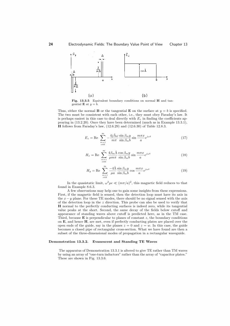

Cite as Markus Zahn course materials for 6641 Electromagnetic Fields Forces and Motion Spring 2005 MIT OpenCourseWare (httpocwmitedu) Massachusetts Institute of Technology Downloaded on [DD Month YYYY]
26 Electrodynamic Fields The Boundary Value Point of View Chapter 13
Fig 1341 Rectangular waveguide
much of what can be expected in pipe waveguides However unlike the parallel plates which can support TEM modes as well as highershyorder TE modes and TM modes the pipe cannot transmit a TEM mode From the parallel plate system we expect that a waveguide will support propagating modes only if the frequency is high enough to make the greater interior crossshysectional dimension of the pipe greater than a free space halfshywavelength Thus we will find that a guide having a larger dimension greater than 5 cm would typically be used to guide energy having a frequency of 3 GHz
We found it convenient to classify twoshydimensional fields as transverse magshynetic (TM) or transverse electric (TE) according to whether E or H was transshyverse to the direction of propagation (or decay) Here where we deal with threeshydimensional fields it will be convenient to classify fields according to whether they have E or H transverse to the axial direction of the guide This classification is used regardless of the crossshysectional geometry of the pipe We choose again the y coordinate as the axis of the guide as shown in Fig 1341 If we focus on solutions to Maxwellrsquos equations taking the form
Hy = Re hy(x z)ej(ωtminuskyy) (1)
Ey = Re ey(x z)ej(ωtminuskyy) (2)
then all of the other complex amplitude field components can be written in terms of the complex amplitudes of these axial fields Hy and Ey This can be seen from substituting fields having the form of (1) and (2) into the transverse components of Amperersquos law (1208)
minusjkyhz minus parth
y = jωex (3)partz
Sec 134 Rectangular Waveguide Modes 27
parth y + jkyh
x = jωez (4)partx
and into the transverse components of Faradayrsquos law (1209)
minusjky ez minus partey = minusjωmicrohx (5)partz
partey + jky ex = minusjωmicrohz (6)partx
If we take h y and ˆ ey as specified (3) and (6) constitute two algebraic equations in
the unknowns ˆ ex and h z Thus they can be solved for these components Similarly
h x and ez follow from (4) and (5)
parth
y partey
h
x = minus jky partx
minus jω (ω2micro minus k2) (7)partz y
h z =
minus jky parth
y + jω partey
(ω2micro minus k2) (8)
partz partx y
ex =
jωmicro parth
y minus jky partey
(ω2micro minus ky
2) (9)partz partx
parthy partˆ ez =
minus jωmicropartx
minus jky ey
(ω2micro minus ky
2) (10)partz
We have found that the threeshydimensional fields are a superposition of those associated with Ey (so that the magnetic field is transverse to the guide axis ) the TM fields and those due to Hy the TE modes The axial field components now play the role of ldquopotentialsrdquo from which the other field components can be derived
We can use the y components of the laws of Ampere and Faraday together with Gaussrsquo law and the divergence law for H to show that the axial complex amplitudes ˆ ey and h
y satisfy the twoshydimensional Helmholtz equations
TM Modes (Hy = 0)
part2ey
partx2 +
part2ey
partz2 + p 2 ey = 0 (11)
where 2 p = ω2micro minus k2
y
and
TE Modes (Ey = 0)
part2hy part2h y+ + q 2h
y = 0 (12)partx2 partz2
28 Electrodynamic Fields The Boundary Value Point of View Chapter 13
where q 2 = ω2micro minus ky
2
These relations also follow from substitution of (1) and (2) into the y components of (1302) and (1301)
The solutions to (11) and (12) must satisfy boundary conditions on the pershyfectly conducting walls Because Ey is parallel to the perfectly conducting walls it must be zero there
TM Modes
ey(0 z) = 0 ey(a z) = 0 ey(x 0) = 0 ey(xw) = 0 (13)
The boundary condition on Hy follows from (9) and (10) which express ex
and ˆ ez in terms of h y On the walls at x = 0 and x = a ez = 0 On the walls at
z = 0 z = w ex = 0 Therefore from (9) and (10) we obtain
TE Modes
parthy (0 z) = 0 parthy (a z) = 0
parthy (x 0) = 0 parthy (x w) = 0 (14)
partx partx partz partz
The derivative of hy with respect to a coordinate perpendicular to the boundary must be zero
The solution to the Helmholtz equation (11) or (12) follows a pattern that is familiar from that used for Laplacersquos equation in Sec 54 Either of the complex amplitudes representing the axial fields is represented by a product solution
ey
ˆ prop X(x)Z(z) (15)hy
Substitution into (11) or (12) and separation of variables then gives
d2X + γ2X = 0 (16)
dx2
d2Z + δ2Z = 0
dz2
where
minusγ2 minus δ2 +
p2
2
= 0 (17)q
Solutions that satisfy the TM boundary conditions (13) are then
TM Modes
mπ X prop sin γmx γm = m = 1 2 (18)
a
29 Sec 134 Rectangular Waveguide Modes
nπ Z prop sin δnz δn = n = 1 2
w
so that pmn 2 =
mπ 2 + nπ 2 m = 1 2 n = 1 2 (19)
a w
When either m or n is zero the field is zero and thus m and n must be equal to an integer equal to or greater than one For a given frequency ω and mode number (mn) the wave number ky is found by using (19) in the definition of p associated with (11)
ky = plusmnβmn
with ⎧ ω2micro minus
mπ
2 minus
nπ 2 2 +
nπ
2⎨ w ω2micro gt
mπ
w (20)βmna a equiv ⎩ minusj
mπ
2 +
nπ 2 minus ω2micro ω2micro lt
mπ
2 +
nπ 2
a w a w
Thus the TM solutions are
infin infin mπ nπ
Ey = Re
(A+ eminusjβmn y + Aminus ejβmn y) sin x sin z ejωt (21)mn mn a w m=1 n=1
For the TE modes (14) provides the boundary conditions and we are led to the solutions
TE Modes
mπ X prop cos γmx γm = m = 0 1 2 (22)
a
nπ Z prop cos δnz δn = n = 0 1 2
a
Substitution of γm and δn into (17) therefore gives
q 2 = mπ 2 +
nπ 2 m = 0 1 2 n = 0 1 2 (23)mn a w
(mn) = (0 0)
The wave number ky is obtained using this eigenvalue in the definition of q assoshyciated with (12) With the understanding that either m or n can now be zero the expression is the same as that for the TM modes (20) However both m and n cannot be zero If they were it follows from (22) that the axial H would be uniform over any given crossshysection of the guide The integral of Faradayrsquos law over the crossshysection of the guide with the enclosing contour C adjacent to the perfectly conducting boundaries as shown in Fig 1342 requires that
E ds = minusmicroA
dHy (24)middot dt
30 Electrodynamic Fields The Boundary Value Point of View Chapter 13
Fig 1342 Crossshysection of guide with contour adjacent to perfectly conshyducting walls
where A is the crossshysectional area of the guide Because the contour on the left is adjacent to the perfectly conducting boundaries the line integral of E must be zero It follows that for the m = 0 n = 0 mode Hy = 0 If there were such a mode it would have both E and H transverse to the guide axis We will show in Sec 142 where TEM modes are considered in general that TEM modes cannot exist within a perfectly conducting pipe
Even though the dispersion equations for the TM and TE modes only differ in the allowed lowest values of (mn) the field distributions of these modes are very different9 The superposition of TE modes gives
infin infin mπ nπ
Re
(C+ eminusjβmn y + Cminus jβmn y) jωt Hy = mn mne cos x cos z e (25) a w
middot m=0 n=0
where m n = 0 The frequency at which a given mode switches from evanescence middot to propagation is an important parameter This cutoff frequency follows from (20) as
1 mπ 2 +
nπ 2 ωc = radic
micro a w (26)
TM Modes m = 0 n = 0
TE Modes m and n not both zero
Rearranging this expression gives the normalized cutoff frequency as functions of the aspect ratio aw of the guide
ωcw ωc equiv
cπ =
(wa)2m2 + n2 (27)
These normalized cutoff frequencies are shown as functions of wa in Fig 1343 The numbering of the modes is standardized The dimension w is chosen as
w le a and the first index m gives the variation of the field along a The TE10
9 In other geometries such as a circular waveguide this coincidence of pmn and qmn is not found
Sec 134 Rectangular Waveguide Modes 31
Fig 1343 Normalized cutoff frequencies for lowest rectangular waveguide modes as a function of aspect ratio
mode then has the lowest cutoff frequency and is called the dominant mode All other modes have higher cutoff frequencies (except of course in the case of the square crossshysection for which TE01 has the same cutoff frequency) Guides are usually designed so that at the frequency of operation only the dominant mode is propagating while all highershyorder modes are ldquocutoffrdquo
In general an excitation of the guide at a crossshysection y = constant excites all waveguide modes The modes with cutoff frequencies higher than the frequency of excitation decay away from the source Only the dominant mode has a sinusoidal dependence upon y and thus possesses fields that are periodic in y and ldquodominaterdquo the field pattern far away from the source at distances larger than the transverse dimensions of the waveguide
Example 1341 TE10 Standing Wave Fields
The section of rectangular guide shown in Fig 1344 is excited somewhere to the right of y = 0 and shorted by a conducting plate in the plane y = 0 We presume that the frequency is above the cutoff frequency for the TE10 mode and that a gt w as shown The frequency of excitation is chosen to be below the cutoff frequency for all higher order modes and the source is far away from y = 0 (ie at y a) The field in the guide is then that of the TE10 mode Thus Hy is given by (25) with m = 1 and n = 0 What is the spaceshytime dependence of the standing waves that result from having shorted the guide
Because of the short Ez(x y = 0 z) = 0 In order to relate the coefficients
C+ and Cminus we must determine ˆ ez from h y as given by (25) using (10) 10 10
a 10e
minusjβ10y jβ10y πx jωt 10eEz = Re jωmicro (C+ + Cminus ) sin e (28)
π a
and because ez = 0 at the short it follows that
C+ = minusCminus (29)10 10
32 Electrodynamic Fields The Boundary Value Point of View Chapter 13
Fig 1344 Fields and surface sources for TE10 mode
so that a π jωt
Ez = 2ωmicro C+ xe (30)Re 10 sin β10y sin
π a
and this is the only component of the electric field in this mode We can now use (29) to evaluate (25)
π jωt
Hy = minusRe 2jC+ cos xe (31)10 sin β10y
a
In using (7) to evaluate the other component of H remember that in the C+ termmn
of (25) ky = βmn while in the Cminus term ky = minusβmnmn
a π jωt
C+Hx = Re 2jβ10 10 cos β10y sin xe (32)
π a
To sketch these fields in the neighborhood of the short and deduce the associshyated surface charge and current densities consider C+ to be real The j in (31) and 10
(32) shows that Hx and Hy are 90 degrees out of phase with the electric field Thus in the field sketches of Fig 1344 E and H are shown at different instants of time say E when ωt = π and H when ωt = π2 The surface charge density is where Ez
terminates and originates on the upper and lower walls The surface current density can be inferred from Amperersquos continuity condition The temporal oscillations of these fields should be pictured with H equal to zero when E peaks and with E equal to zero when H peaks At planes spaced by multiples of a halfshywavelength along the y axis E is always zero
Sec 135 Optical Fibers 33
Fig 1345 Slotted line for measuring axial distribution of TE10 fields
The following demonstration illustrates how a movable probe designed to coushyple to the electric field is introduced into a waveguide with minimal disturbance of the wall currents
Demonstration 1341 Probing the TE10 Mode
A waveguide slotted line is shown in Fig 1345 Here the line is shorted at y = 0 and excited at the right The probe used to excite the guide is of the capacitive type positioned so that charges induced on its tip couple to the lines of electric field shown in Fig 1344 This electrical coupling is an alternative to the magnetic coupling used for the TE mode in Demonstration 1332
The y dependence of the field pattern is detected in the apparatus shown in Fig 1345 by means of a second capacitive electrode introduced through a slot so that it can be moved in the y direction and not perturb the field ie the wall is cut along the lines of the surface current K From the sketch of K given in Fig 1344 it can be seen that K is in the y direction along the center line of the guide
The probe can be used to measure the wavelength 2πky of the standing waves by measuring the distance between nulls in the output signal (between nulls in Ez) With the frequency somewhat below the cutoff of the TE10 mode the spatial decay away from the source of the evanescent wave also can be detected
135 DIELECTRIC WAVEGUIDES OPTICAL FIBERS
Waves can be guided by dielectric rods or slabs and the fields of these waves occupy the space within and around these dielectric structures Especially at optical wavelengths dielectric fibers are commonly used to guide waves In this section we develop the properties of waves guided by a planar sheet of dielectric material The waves that we find are typical of those found in integrated optical systems and in the more commonly used optical fibers of circular crossshysection
A planar version of a dielectric waveguide is pictured in Fig 1351 A dielectric of thickness 2d and permittivity i is surrounded by a dielectric of permittivity lt i The latter might be free space with = o We are interested in how this
34 Electrodynamic Fields The Boundary Value Point of View Chapter 13
Fig 1351 Dielectric slab waveguide
structure might be used to guide waves in the y direction and will confine ourselves to fields that are independent of z
With a source somewhere to the left (for example an antenna imbedded in the dielectric) there is reason to expect that there are fields outside as well as inside the dielectric We shall look for field solutions that propagate in the y direction and possess fields solely inside and near the layer The fields external to the layer decay to zero in the plusmnx directions Like the waves propagating along waveguides those guided by this structure have transverse components that take the form
Ez = Re ˆ ez(x)ej(ωtminuskyy) (1)
both inside and outside the dielectric That is the fields inside and outside the dielectric have the same frequency ω the same phase velocity ωky and hence the same wavelength 2πky in the y direction Of course whether such fields can actually exist will be determined by the following analysis
The classification of twoshydimensional fields introduced in Sec 126 is applicashyble here The TM and TE fields can be made to independently satisfy the boundary conditions so that the resulting modes can be classified as TM or TE10 Here we will confine ourselves to the transverse electric modes In the exterior and interior regions where the permittivities are uniform but different it follows from substishytution of (1) into (12633) (Table 1283) that
d2ez minus α2 xez = 0 αx =
ky
2 minus ω2micro d lt x and x lt minusd (2)dx2
d2ez + k2 ez = 0 kx =
ω2microi minus k2 minusd lt x lt d (3)dx2 x y
A guided wave is one that is composed of a nonuniform plane wave in the exterior regions decaying in the plusmnx directions and propagating with the phase velocity ωky in the y direction In anticipation of this we have written (2) in
10 Circular dielectric rods do not support simple TE or TM waves in that case this classifishycation of modes is not possible
Sec 135 Optical Fibers 35
terms of the parameter αx which must then be real and positive Through the continuity conditions the exterior wave must match up to the interior wave at the dielectric surfaces The solutions to (3) are sines and cosines if kx is real In order to match the interior fields onto the nonuniform plane waves on both sides of the guide it is necessary that kx be real
We now set out to find the wave numbers ky that not only satisfy the wave equations in each of the regions represented by (2) and (3) but the continuity conditions at the interfaces as well The configuration is symmetric about the x = 0 plane so we can further divide the modes into those that have even and odd functions Ez(x) Thus with A an arbitrary factor appropriate even solutions to (2) and (3) are ⎧
⎪⎪⎨
⎪⎪⎩
Aeminusαx(xminusd) d lt x cos kxx
ez = A minusd lt x lt d (4)cos kxd
Aeαx(x+d) x lt minusd
To simplify the algebra we have displaced the origin in the exterior solutions so that just the coefficient A is obtained when ez is evaluated at the respective interfaces With a similar objective the interior solution has been divided by the constant cos(kxd) so that at the boundaries ez also becomes A In this way we have adjusted the interior coefficient so that ez is continuous at the boundaries
Because this transverse field is the only component of E all of the continuity conditions on E are now satisfied The permeabilities of all regions are presumed to be the same so both tangential and normal components of H must be continuous at the boundaries From (12629) the continuity of normal microH is guaranteed by the continuity of Ez in any case The tangential field is obtained using (12630)
h y =
1 dez (5)jωmicro dx
Substitution of (4) into (5) gives
hy = 1
jωmicro
⎧⎨
⎩
minusα Aeminusαx(xminusd) d lt x minusk
x
A sin kxx minusd lt x lt d (6)cos kxdx
αxAeαx(x+d) x lt minusd
The assumption that Ez is even in x has as a consequence the fact that the continushyity condition on tangential H is satisfied by the same relation at both boundaries
αx minusαxA = minuskxA tan kxd rArr kx
= tan kxd (7)
Our goal is to determine the propagation constant ky for a given ω If we were to substitute the definitions of αx and kx into this expression we would have this dispersion equation D(ωky) implicitly relating ky to ω It is more convenient to solve for αx and kx first and then for ky
Elimination of ky between the expressions for αx and kx given with (2) and (3) gives a second expression for αxkx
αx =
ω2microid2
1minus minus 1 (8)
kx (kxd)2 i
36 Electrodynamic Fields The Boundary Value Point of View Chapter 13
Fig 1352 Graphical solution to (7) and (8)
The solutions for the values of the normalized transverse wave numbers (kxd) can be pictured as shown in Fig 1352 Plotted as functions of kxd are the rightshyhand sides of (7) and (8) The points of intersection kxd = γm are the desired solutions For the frequency used to make Fig 1352 there are two solutions These are designated by even integers because the odd modes (Prob 1351) have roots that interleave these even modes
As the frequency is raised an additional even TEshyguided mode is found each time the curve representing (8) reaches a new branch of (7) This happens at freshyquencies ωc such that αxkx = 0 and kxd = mπ2 where m = 0 2 4 From (8)
mπ 1 ωc = (9)
2d
micro(i minus )
The m = 0 mode has no cutoff frequency To finally determine ky from these eigenvalues the definition of kx given with
(3) is used to write kyd =
ω2microid2 minus (kxd)2 (10)
and the dispersion equation takes the graphical form of Fig 1353 To make Fig 1352 we had to specify the ratio of permittivities so that ratio is also implicit in Fig 1353
Features of the dispersion diagram Fig 1353 can be gathered rather simply Where a mode is just cutoff because ω = ωc αx = 0 as can be seen from Fig 1352 From (2) we gather that ky = ωc
radicmicro Thus at cutoff a mode must have a
propagation constant ky that lies on the straight broken line to the left shown in Fig 1353 At cutoff each mode has a phase velocity equal to that of a plane wave in the medium exterior to the layer
In the highshyfrequency limit where ω goes to infinity we see from Fig 1352 that kxd approaches the constant kx (m + 1)π2d That is in (3) kx becomes a rarrconstant even as ω goes to infinity and it follows that in this high frequency limit ky ω
radicmicroi rarr
Sec 135 Optical Fibers 37
Fig 1353 Dispersion equation for even TE modes with i = 66
Fig 1354 Distribution of transverse E for TE0 mode on dielectric wavegshyuide of Fig 1351
The physical reasons for this behavior follow from the nature of the mode pattern as a function of frequency When αx 0 as the frequency approaches rarrcutoff it follows from (4) that the fields extend far into the regions outside of the layer The wave approaches an infinite parallel plane wave having a propagation constant that is hardly affected by the layer In the opposite extreme where ω goes to infinity the decay of the external field is rapid and a given mode is well confined inside the layer Again the wave assumes the character of an infinite parallel plane wave but in this limit one that propagates with the phase velocity of a plane wave in a medium with the dielectric constant of the layer
The distribution of Ez of the m = 0 mode at one frequency is shown in Fig 1354 As the frequency is raised each mode becomes more confined to the layer
38 Electrodynamic Fields The Boundary Value Point of View Chapter 13
Fig 1355 Dielectric waveguide demonstration
Demonstration 1351 Microwave Dielectric Guided Waves
In the experiment shown in Fig 1355 a dielectric slab is demonstrated to guide microwaves To assure the excitation of only an m = 0 TEshyguided wave but one as well confined to the dielectric as possible the frequency is made just under the cutoff frequency ωc2 (For a 2 cm thick slab having io = 66 this is a frequency just under 6 GHz) The m = 0 wave is excited in the dielectric slab by means of a vertical element at its left edge This assures excitation of Ez while having the symmetry necessary to avoid excitation of the odd modes
The antenna is mounted at the center of a metal ground plane Thus without the slab the signal at the receiving antenna (which is oriented to be sensitive to Ez) is essentially the same in all directions perpendicular to the z axis With the slab a sharply increased signal in the vicinity of the right edge of the slab gives qualitative evidence of the wave guidance The receiving antenna can also be used to probe the field decay in the x direction and to see that this decay increases with frequency11
136 SUMMARY
There are two perspectives from which this chapter can be reviewed First it can be viewed as a sequence of specific examples that are useful for dealing with radio frequency microwave and optical systems Secs 131ndash133 are concerned with the propagation of energy along parallel plates first acting as a transmission line and then as a waveguide Practical systems to which the derived properties of the TEM and highershyorder modes are directly applicable are strip lines used at frequencies
11 To make the excitation independent of z a collinear array of inshyphase dipoles could be used for the excitation This is not necessary to demonstrate the qualitative features of the guide
Cite as Markus Zahn course materials for 6641 Electromagnetic Fields Forces and Motion Spring 2005 MIT OpenCourseWare (httpocwmitedu) Massachusetts Institute of Technology Downloaded on [DD Month YYYY]
Sec 136 Summary 39
that extend from dc to the microwave range The rectangular waveguide of Sec 134 might well be a section of ldquoplumbingrdquo from a microwave communication system and the dielectric waveguide of Sec 135 has many of the properties of an optical fiber Second the mathematical analysis of waves exemplified in this chapter is generally applicable to other more complex systems that are uniform in one direction
When the structures described in this chapter are used to transport energy from one location to another they are generally not terminated in ldquoshortsrdquo and ldquoopensrdquo and hence generally do not simply support standing waves The object is usually to carry energy from an antenna to a receiver or from a generator to a load whether that be an antenna or a light bulb Such energy transport is accomplished by the traveling waves featured in the next chapter
40 Electrodynamic Fields The Boundary Value Point of View Chapter 13
P R O B L E M S
131 Introduction to TEM Waves
1311lowast With a short at y = 0 it is possible to find the fields for Example 1311 by recognizing at the outset that standing wave solutions meeting the homogeshyneous boundary condition of (12) are of the form Ex = Re A sin(βy) exp(jωt)
(a) Use (1312) and (1313) to determine the associated Hz and the dispersion equation (relation between β and ω)
(b) Now use the boundary condition at y = minusb to show that the fields are as given by (13116) and (13117)
1312lowast Take the approach outlined in Prob 1311 for finding the fields [(13128) and (13129)] in Example 1312
1313 Assume that K o is real and express the standing wave of (13117) so as
to make it evident that it is the sum of equalshyamplitude waves traveling in the plusmny directions each with a magnitude of phase velocity ωβ = c and wavelength 2πβ
1314lowast Coaxial perfectly conducting circular cylinders having outer and inner radii a and b respectively form the transmission line shown in Fig P1314
(a) If the conductors were ldquoopen circuitrdquo at z = 0 and driven by a voltage source V at z = minusl show that the EQS electric field is radial and given by V[r ln(ab)]
(b) If the conductors were ldquoshortedrdquo at z = 0 and driven by a current source I at z = minusl show that the MQS magnetic field intensity is φ directed and given by I2πr
(c) With the motivation provided by these limiting solutions show that solutions to all of Maxwellrsquos equations (in the region between the conductors) that satisfy the boundary conditions on the surfaces of the coaxial conductors are
V (z t) I(z t)E = ir
ln
ab
r H = iφ 2πr
(a)
provided that V and I are now functions not only of t but of z as well that satisfy equations taking the same form as (1312) and (1313)
partI partV 2π
partz = minusC
partt C equiv
ln
a (b)
b
partV partI ln
ab
micro
partz = minusL
partt L equiv
2π (c)
Sec 132 Problems 41
Fig P1314
1315 For the coaxial configuration of Prob 1314 there is a perfectly conducting ldquoshortrdquo at z = 0 and the conductors are driven by a current source I = Re[Ioe
jωt] at z = minusl
(a) Find I(z t) and V (z t) and hence E and H (b) Take the low frequency limit where ω
radicmicrol 1 and show that E and
H are the same as for a coaxial inductor (c) Find E and H directly from the MQS laws and show that they agree
with the results of part (b)
1316 For the coaxial configuration of Prob 1314 the conductors are ldquoopen circuitedrdquo at z = 0 and driven by a voltage source V = Re [Vo exp(jωt] at x = minusl
(a) Find I(z t) and V (z t) and hence E and H (b) Take the lowshyfrequency limit where ω
radicmicrol 1 and show that E and
H are the same as for a coaxial capacitor (c) Find E and H directly from the EQS laws and show that they agree
with the results of (b)
132 TwoshyDimensional Modes Between Parallel Plates
1321lowast Show that each of the highershyorder modes propagating in the +y direcshytion represented by A+
n and Cn + in (13219) and (13220) respectively
can be regarded as the sum of plane waves propagating in the directions represented by the vector wave number
nπk = + βn (a)plusmn
a ix iy
and interfering in the planes x = 0 and x = a so as to satisfy the boundary conditions
1322 The TM and TE modes can themselves be classified into odd or even modes that respectively have h
z or ˆ ez odd or even functions of x With this in mind the origin of the coordinate system is moved so that it is midway between the perfectly conducting plates as shown in Fig P1322
42 Electrodynamic Fields The Boundary Value Point of View Chapter 13
Fig P1322
(a) Find the odd TM and TE solutions Note that when the boundary condition is met at x = d equiv a2 for these functions it is automatically met at x = minusd
(b) Find the even TM and TE solutions again noting that if the condishytions are met at x = d then they are at x = minusd as well
133 TE and TM Standing Waves between Parallel Plates
1331lowast Starting with (1331) (for TM modes) and (1332) (for TE modes) use steps similar to those illustrated by (5520)ndash(5526) to obtain the orthogshyonality conditions of (1333) and (1334) respectively
1332 In the system of Example 1331 the wall at y = 0 is replaced by that shown in Fig P1332 A strip electrode is embedded in but insulated from the wall at y = 0 The resistance R is low enough so that E tangential to the boundary at y = 0 even at the insulating gaps between the strip electrode and the surrounding wall is negligible
(a) Determine the output voltage vo in terms of v (b) For ba = 2 describe the dependence of vo on frequency over the | |
range ωradic
micro a = 0 π
54 specifying the lowshyfrequency range where the response
rarrhas a linear dependence on frequency and the
resonance frequencies (c) What is the distribution of Hz(x y) at the resonance frequencies
1333lowast In the twoshydimensional system of Fig P1333 each driven electrode has the same nature as the one in Fig 1331 The origin of the y axis has been chosen to be in the plane of symmetry
(a) Use the symmetry to argue that Hz(y = 0) = 0
Sec 133 Problems 43
Fig P1332
Fig P1333
(b) Show that in the interior region
infin minus4jωv sin βny nπx jωt Hz = Re
cos e (a)βna cos βnb a
n=1 odd
1334 The oneshyturn loop of Fig P1334 has dimensions that are small compared to a b or wavelengths of interest and has area A in the x minus y plane
(a) It is used to detect the TM H field at the middle of the bottom electrode in Fig 1331 Assume that the resistance is large enough so that the current induced in this loop gives rise to a magnetic field that is negligible compared to that already found In terms of Hz what is vo
(b) At what locations x = X of the loop is a maximum |vo|(c) If the same loop were in the plate at y = 0 in the configuration of Fig
1313 and used to detect Hz at y = 0 for the TEM fields of Example
44 Electrodynamic Fields The Boundary Value Point of View Chapter 13
Fig P1334
1311 what would be the dependence of vo on the location x = X of the loop
| |
(d) If the loop were located in the plate at y = 0 in the TE configuration of Fig 1334 how should the loop be oriented to detect H
1335 In the system shown in Fig P1335 Δ d and the driving sources v = Re[v exp(jωt)] are uniformly distributed in the z direction so that the fields are two dimensional Thus the driving electrode is like that of Fig 1331 except that it spans the width d rather than the full width a Find H and E in terms of v
1336 In the system shown in Fig P1336 the excitation electrode is like that for Fig 1334 except that it has a width d rather than a Find H and E in terms of Λ
134 Rectangular Waveguide Modes
1341lowast Show that an alternative method of exciting and detecting the TE10 mode in Demonstration 1341 is to introduce oneshyturn loops as shown in Fig P1341 The excitation loop is inserted through a hole in the conducting wall while the detection loop passes through a slot so that it can be moved in the y direction The loops are each in the y minus z plane To minimize disturbance of the field the detection loop is terminated in a high enough impedance so that the field from the current in the loop is negligible Comshypare the y dependence of the detected signal to that measured using the electric probe
1342 A rectangular waveguide has wa = 075 Presuming that all TE and TM modes are excited in the guide in what order do the lowest six modes begin to propagate in the y direction as the frequency is raised
1343lowast The rectangular waveguide shown in Fig P1343 is terminated in a pershyfectly conducting plate at y = 0 that makes contact with the guide walls An electrode at y = b has a gap of width Δ a and Δ w around its
45 Sec 134 Problems
Fig P1335
Fig P1336
Fig P1341
edges Distributed around this gap are sources that constrain the field from the edges of the plate to the guide walls to v(t)Δ = Re(vΔ) exp(jωt)
(a) Argue that the fields should be TM and use the boundary condition
46 Electrodynamic Fields The Boundary Value Point of View Chapter 13
Fig P1343
at y = 0 to show that
infin infin mπ nπˆ
2A+Ey = mn cos βmny sin x sin z (a)
a w m=1 n=1
[Hint If (1349) and (13410) are used remember that ky = +βmn
for the A+ mn mode but ky = minusβmn for the Aminus mode ] mn
(b) Show that for m and n both odd A+ = 8ˆ v(ω2microminusβ2 )nmπ2βmn sin(kmnb)mn mnwhile for either m or n even A+ = 0mn
(c) Show that for these modes the resonance frequencies (normalized to 1radic
microa) are
ωradic
microa = π
m2 + a
n2 +
ap2 (b)
w b
where m n and p are integers m and n odd (d) Show that under quasistatic conditions the field which has been found
is consistent with that implied by the EQS potential given by (51010) and (51015)
1344 The rectangular waveguide shown in Fig P1343 is terminated in a pershyfectly conducting plate at y = 0 that makes contact with the guide walls However instead of the excitation electrode shown at y = b there is the perfectly conducting plate with a square hole cut in its center shown in Fig P1344 In this hole the pole faces of a magnetic circuit are flush with the plate and are used to excite fields within the guide Approximate the normal fields over the surface of the pole faces as
H
o for a lt x lt a+Δ and wminusΔ lt z lt w+Δ
Hy = 2 2 2 2 (a)w+ΔminusH
o for aminus2Δ lt x lt a
2 and wminus2Δ lt z lt 2
Sec 135 Problems 47
Fig P1344
where Ho is a complex constant (Note that if the magnetic circuit is driven by a one turn coil the terminal voltage v = jω(Δ22)microH
o) Determine Hy and hence E and H inside the guide
135 Dielectric Waveguides Optical Fibers
1351lowast For the dielectric slab waveguide of Fig 1351 consider the TE modes that have Ez an odd function of z
(a) Show that the dispersion relation between ω and ky is again found from (13510) but with (kxd) found by simultaneously solving (1358) and
αx = minus cot kxd (a)kx
(b) Sketch the graphical solution for kxd equiv γm (m odd) and show that the cutoff frequency is again given by (1359) but with m odd rather than even
(c) Show that these odd modes also have the asymptote of unity slope shown in Fig 1353
(d) Sketch the odd mode dispersion relation on that for the even modes (Fig 1353)
1352 For the dielectric slab waveguide shown in Fig 1351 i = 25 micro = microo and d = 1 cm In Hz what is the highest frequency that can be used to guide only one TE mode (Note the result of Prob 1351)
1353lowast The dielectric slab waveguide of Fig 1351 is the same as that considered in this problem except that it now has a permeability microi that differs from that outside where it is micro
(a) Show that (1357) and (1358) respectively are replaced by
αx = micro
tan kxd
even (a)
kx microi minus cot kxd odd
48 Electrodynamic Fields The Boundary Value Point of View Chapter 13
αx =
ω2microiid2
1minus micro minus 1
kx (kxd)2 microii (b)
(b) Show that making microi gt micro lowers the cutoff frequency (c) For a given frequency does making microimicro gt 1 increase or decrease the
wavelength λ equiv 2πky
1354 The dielectric slab of Fig 1351 has permittivity i and permeability microi while in the surrounding regions these are and micro respectively Consider the TM modes
(a) Determine expressions analogous to (1357) (1358) and (13510) that can be used to determine the dispersion relation ω = ω(ky) for modes that have Hz even and odd functions of x
(b) What are the cutoff frequencies (c) For microi = micro and i = = 25 draw the dispersion plot for the lowest
three modes that is analogous to that of Fig 1353
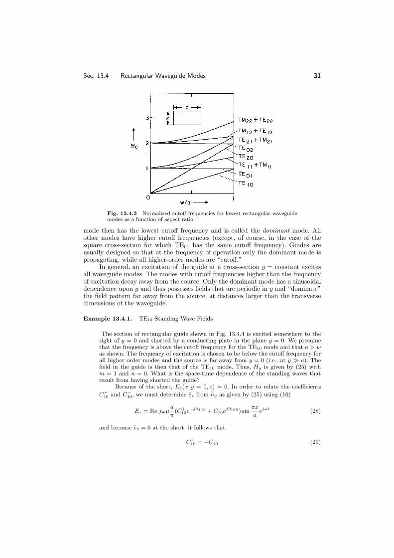
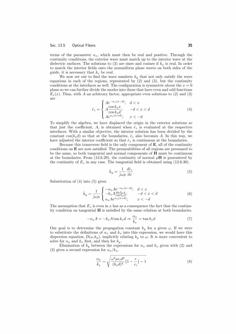
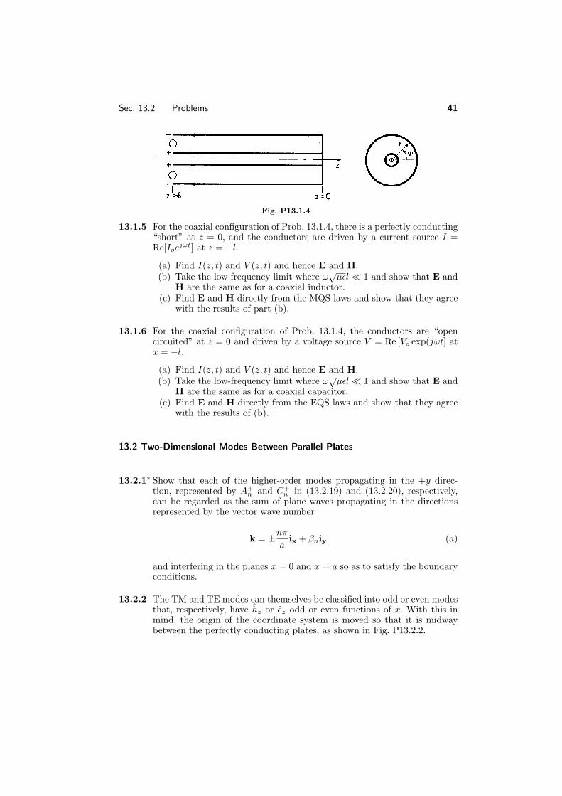
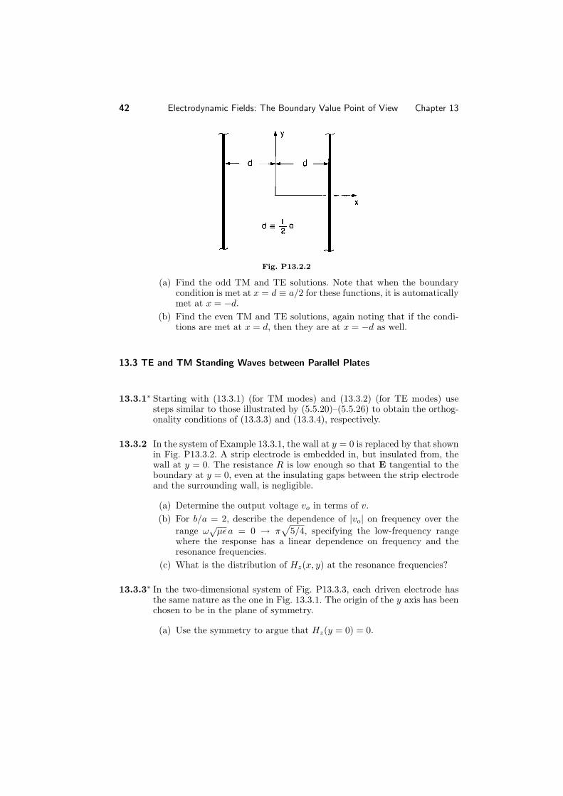
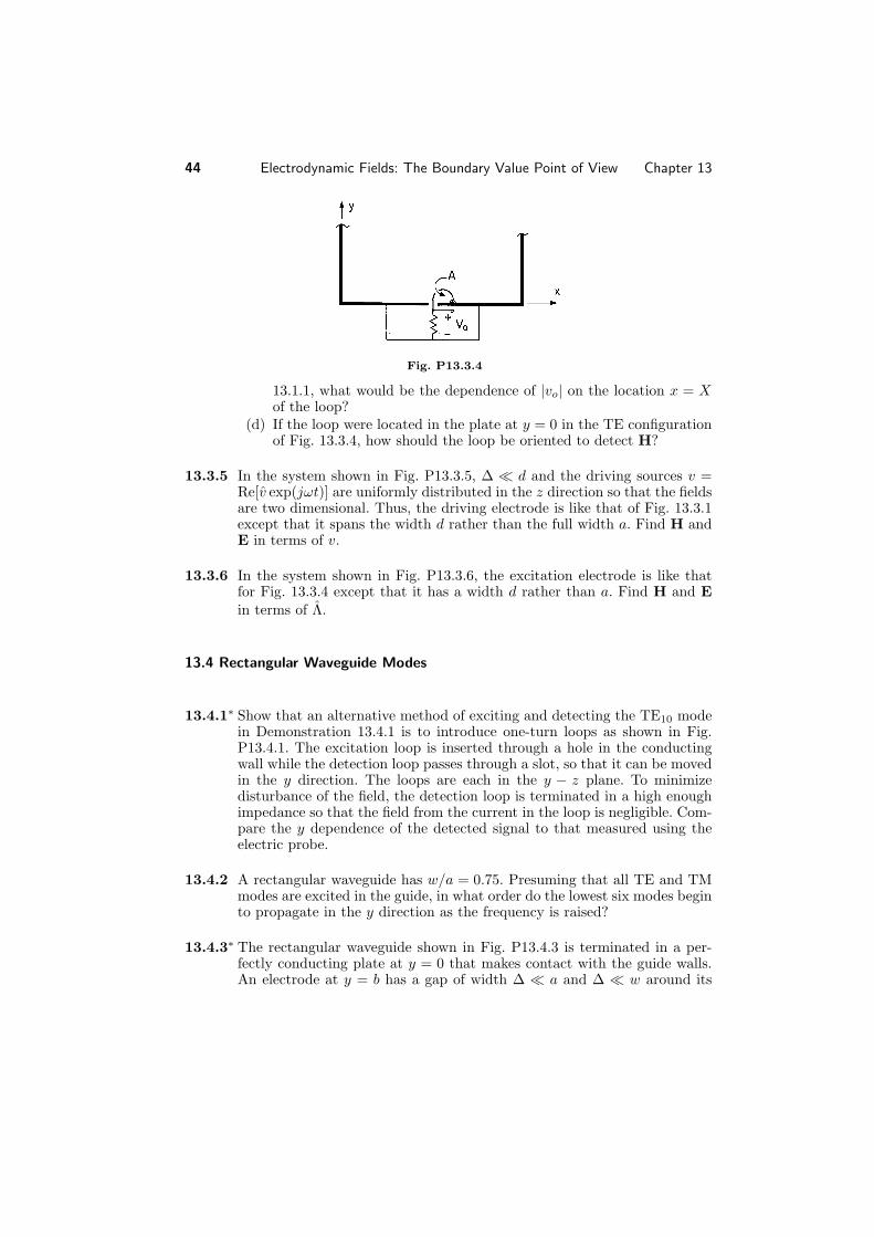
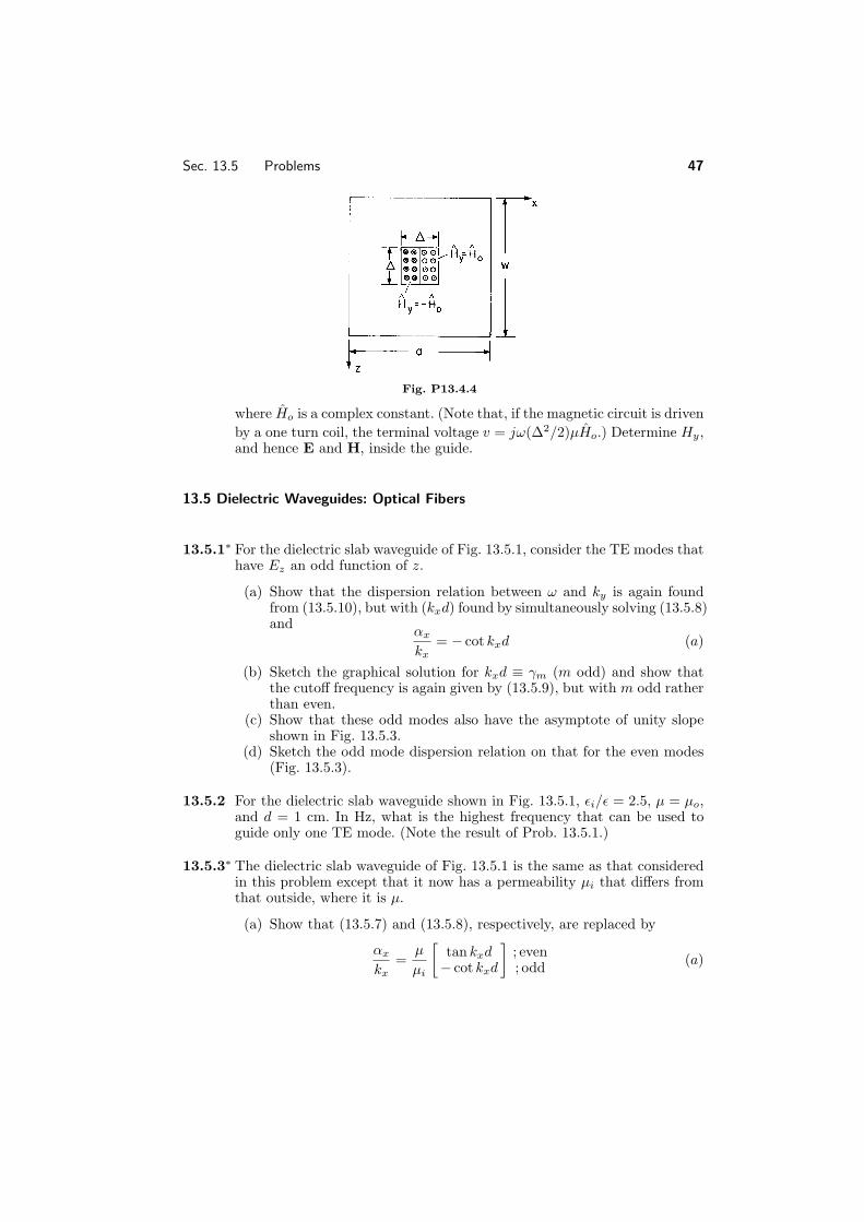