Electromagnetic Field Coupling to Transmission Lines...

1

Interaction Notes Note 623 30 June 2011

Electromagnetic Field Coupling to Transmission Lines Inside Rectangular Resonators

S. Tkachenko*, J. Nitsch*, and R. Rambousky** *Otto-von-Guericke-University-Magdeburg

**Bundeswehr Research Institute for Protective Technologies and NBC Protection Abstract In this paper the current inside a cavity, which is induced by lumped and distributed sources, is calculated. The current is obtained analytically (Green’s function method) and numerically (MoM – and MLFMM – method). A long, parallel wire is chosen that connects two opposite walls of a rectangular resonator. Since the conductor conserves the translational symmetry of the resonator in one direction (z-direction), the current and the total exciting electrical field can be derived from Fourier series formulations. The obtained results clearly show the influence of the resonator on the induced current. Resonance peaks of the resonator, which do not arise in usual EMC laboratory tests, occur in the current spectra. The numerical results agree very well with the analytical ones, however, the results are obtained much faster using the analytical formulae - by a factor of one thousand. _________________________________________________________________________ This work was sponsored by the German Research Foundation (DFG) under the contract number:NI 633/5-1

2

Contents Page

1. Introduction 3 2. Electromagnetic field coupling to a short-circuited thin wire maintaining the symmetry of the rectangular resonator 4 2.1 Resonator Green’s functions 5

2.2 Calculation of the current 7

2.3 Determination of the function ),( �� S 8

3. Lumped and distributed sources (loads) 10 4. Transmission line approximation 13 5. Comparison of analytical and numerical results 15 6. Conclusion 18 References 19 Appendix I 21 Appendix II 25 Appendix III 26

3

1. Introduction The performance of immunity tests according to current EMC standards on devices under laboratory conditions guarantees a certain basic protection for them. However, ultimately, these devices are used/installed in environments which do not correspond to the test environment in the laboratory. For example, they may be housed in shielded rooms and/or be connected in larger overall systems with other electrical and electronic components. In such cases, compliance of EMC standards for single devices/components does not mean EMC robustness of the total system, because in this system electromagnetic coupling may occur that was not present in the individual tests. In this paper this fact will be demonstrated analytically and numerically in a manageable, but not simple example. Coupling of electromagnetic fields to different transmission-lines and antenna-like wiring structures is one of the main paths of interaction of intentional and natural electromagnetic interferences with electronic and electrical equipment. Usually such problems are considered for objects in free space [1], however, often such structures are inside resonator-like structures of a different kind (racks, cases, housings, fuselage of aircraft, etc.). Then, due to the presence of the resonator, the interaction can change greatly. Existing numerical methods (Method of Moments (MoM), Transmission-Line Matrix Method (TLM), etc.) allow considering specific cases only, but do not describe the general physical picture of the interaction. Thus, the analytical description of the interaction of high-frequency fields with wire structures in cavities has become a topic of interest (see, for example, [2]). To solve this problem several methods can be offered. The approximate methods are based, as is usual in theoretical physics, on the use of small parameters. One group of such methods uses the smallness of the dimension of the wiring structure in comparison to the wavelength. This leads to the description of common modes of the scattered current with the aid of the model of small electrical dipole antennas [3, 4, 5] and to the differential modes of the scattered current using the method of small magnetic loop antennas [6]. The mutual influence of antenna and cavity modes increases with the length of the antenna. This influence can be quantitatively characterized by a shift of the resonance frequency of the system “antenna in cavity” in comparison with the resonance frequency of the empty cavity. It is proportional to the cube of the ratio of linear dimensions of the antenna and the cavity. Therefore, it follows that the maximal electromagnetic coupling occurs when the size of the antenna or transmission line is about the same size as the cavity. Of course, for such a large extension of the scatterers, the “Method of Small Antenna” is not applicable. Another small parameter that can be used to solve the coupling problem for electrically long antennas and transmission lines inside a resonator is the thickness of the wire compared to other geometric parameters of the problem (wavelength, height of the wire above ground, etc.) [7]. The relevant mathematical technique is the method of analytical regularization [8] where the approximate resolution operator for the singular part of the Green’s function is given by the transmission line approximation, and the regular part of the Green’s function is defined by one or more eigenmodes of the cavity. This approach allows considering the coupling of electromagnetic fields with electrically long transmission lines and antennas of arbitrary geometric configuration inside the resonator, when the frequency is close to one of the resonance frequencies and all the other modes of the resonator contribute to form the singular part of the cavity’s Green’s function. This method was verified by comparison with results of the TLM method and yielded an acceptable agreement [7].

4

Further, in the publications [9,10,11] the method of analytical regularization is applied in implicit form. The authors of Ref. [9] only take the singular part of the cavity’s Green’s function in transmission-line approximation into account. This is also done in Ref. [10], but a finite sum of modes in the waveguide representation is chosen for the regular part of the Green’s function. It is interesting to check the method of Ref. [7] by comparing the results with the exact solution and to investigate the structure of the exact solution, even for special cases. Moreover, the problem can be used to investigate the change of the quality factor of the resonator caused by the presence of loaded transmission lines [12]. In this paper, for the exact solution of this problem a technique of theoretical physics is used for the investigation of a “wire in resonator” system that has high symmetry. This system consists of a rectangular resonator and an internal wire parallel to a resonator axis connecting opposite walls of the resonator. The wire can be loaded in an appropriate way (including two lumped loads near the terminals). Moreover, the method allows considering a finite number of such parallel (or perpendicular) wires. The electric field integral equation or mixed potential integral equation (using only the thin-wire approximation), which describes the induced current in such wires, can be solved by a Fourier transformation. The advantage of this geometry of the system leads to the similarity of the Fourier series expansion functions for the induced current and of the Fourier series expansion functions for the resonator Green’s function in the direction of the wire. Moreover, during the investigation of the exact equation for the induced current one can separate terms corresponding to the transmission line approximation from those corresponding to cavity modes and evaluate the effect of different resonances. The results of the analytical investigations were compared to numerical ones (MoM and Multi-Level Fast Multi-Pole Method (MLFMM) calculations) and a good agreement was found. In conclusion, possible directions of future research are described. As is typical in theoretical physics, after using symmetry properties for some specific system one can generalize the results using a topological approach [13]. Note that from a topological point of view, the investigated transmission line with symmetric geometry is equivalent to a usual transmission line inside the resonator. 2. Electromagnetic field coupling to a short-circuited thin wire maintaining the symmetry of the rectangular resonator Consider a rectangular resonator with dimensions hba ,, (see Fig.1). In the resonator there is a wire that is parallel to four resonator walls and is perpendicular to the other two walls. The length of the wire L is equal to the distance h between the latter walls. Thus, the wire has the same geometric symmetry as the rectangular cavity. The wire can be loaded or (and) may have lumped sources localized near the walls. It is assumed that the radius of the wire, 0r , is small in comparison with all other dimensions of the problem (characteristic wavelength � , dimensions of the resonator and distance between the wire and parallel walls).

5

Fig. 1: Loaded symmetrical wire in the rectangular resonator with the parameters:

a=1.5 m, b=1.2 m, h=0.9 m. Length of the line L=h=0.9 m, position of the line x0=0.09 m, y0=0.37 m, and r0=1mm It is also assumed that in the empty resonator (when the wire is absent) an electromagnetic field )(0 rE ��

is created in some way, e.g., by radiation of an additional antenna, the penetration of an external field through the slots and apertures of the cavity, etc. If the sources (current in the radiating antenna, dipole moments of the aperture, which can be treated as a current distribution) are known, the field in the resonator can be calculated by the Green’s function formulation. A central point in this paper is the calculation of the induced current I(z) along the conductor in the resonator. In order to achieve this, some intermediate steps are necessary. 2.1 Resonator Green’s functions Due to the assumed symmetrical wire configuration in the resonator, only the zz components of the dyadic Green’s functions are relevant for the calculations here. This applies to the Green’s function of the vector potential A

� and for the scattered electric field ),( rrE sc

zz �� in the

ray – representation [14, 15]

��

��

��

��321

21

,, 321

3210

|),,(||)),,(|exp()1(

4),(

nnn

nnAzz nnnRr

nnnRrjkRrG ��

��

�

(1)

with � )(),(),(),,( 321321 nZnYnXnnnR �

�

anxnXn

n��

��

�

�� 111 2

)1(1)1()(1

1

bnynYn

n��

��

�

�� 212 2

)1(1)1()(2

2 (2)

hnznZn

n��

��

�

�� 313 2

)1(1)1()(3

3

The coordinates 1x , 1y , 1z denote a point inside the resonator which is reflected

1n , 2n , 3n times at the resonator’s walls in x , y , and z directions, respectively.

6

It can be shown that after some calculations – similar to those which have been performed in Ref. [16] - A

zzG can be expressed as:

3

1 23

,0 1 1 101 2 2

, 10

sin( )sin( )sin( )sin( ) cos( ) cos( )4( , ) n vx vx vy vy vz vzAzz

n n vn

k x k x k y k y k z k zG r r

V k k j��

�

�

��

�� (3)

with the abbreviations V abh� ,

),,( vzvyvxv kkkk ��

, 1na

kvx

� , 2nb

kvy

� , 3vzk nh

� (4)

321 ,,: nnnv � , 0�� , ��

��

�nmnm

mn ,2,1

,�

The index � denotes an eigenstate (mode), e.g. 011TE , of the resonator. The bracket is adopted from quantum mechanics. The quantity � in the denominator is introduced in order to avoid singularities at the eigenfrequencies. It is mathematically necessary if eq. (7) would be transformed into time domain. Then, for the integration, the appropriate contour goes around the singularity, and � is the distance of the contour to the pole. In a physical sense � can be assigned to small losses in the resonator, like, e.g. losses in the walls. In any case it has the same dimension as 2k . It can further be shown that the above summation over three indices can be reduced and simplified to a sum over two. The vector potential Green’s function AG of the resonator is connected with the dyadic Green’s function of the electric field [17] via the equation

� ),(ˆ1),(ˆ 2

0

rrGdivgradkj

rrG Arr

E ��

�� (5)

Therefore, for the zz – component E

zzG it follows

),(),( 2

220 rrG

zk

jkcrrG A

zzEzz ��

�

��

��

�� (6)

Here c denotes the speed of light and 000 �� . Inserting eq. (3) into eq. (6) and performing the differentiation leads to

��

��

��

01,

22111

220,0

1

321

3)cos()cos()sin()sin()sin()sin()(4),(

nnn v

vzvzvyvyvxvxvznEzz jkk

zkzkykykxkxkkkjkV

rrG�

��

(7)

By virtue of the chosen symmetry of the conductor relative to the resonator walls the zz – component of the Green’s function EG is sufficient to calculate the (scattered) current along

7

the line. If the exciting field )(0 rE �� inside the resonator is known, then the induced (scattered)

current )(zI is related to scattered electric field by

zdzIrrGrEh

Ezz

scz �� )(),()(

0

�� (8)

And, in addition to the boundary conditions on the surface of the conductor for the total electric field, the current can be calculated. 2.2 Calculation of the current It is assumed that both ends of the conductor are directly connected with the corresponding walls, i.e. the conductor is short circuited at both ends. Furthermore, only the component of the exciting field parallel to the conductor 0

zE couples to the line, and it also has to fulfill the boundary conditions on the resonator walls. For this reason, it factorizes with respect to its coordinates as follows:

��

�

�0

300

3

3)/cos(),()(

nnzz hznyxErE �

(9)

If one additionally uses the fact that the conductor is short – circuited, the current can be written as

��

�

�0

33

3)/cos()(

nn hznIzI (10)

and one immediately obtains 0|/|/ 0 �� hzz dzdIdzdI . On the basis of equations (9) and (10) together with the boundary condition for the total electrical field on the surface of the conductor1

� � 0,,,, 000

0000 � zyrxEzyrxE z

scz , (here 0r is the radius of the wire) (11)

one can derive the unknown expansion components

3nI for the current. This is carried out in

the next step. Remember � zyrxE scz ,, 000 is given by

zdzIzyxyrxGzyrxEh

Ezz

scz �� )(),,,,(),,( 00000

0000 (12)

1 For the derivation the thin – wire approximation is used. Then, the radius of the wire is much smaller than all other characteristic lengths of the problem: wavelength, length of the wire, distances from the wire to the walls of the resonator. In this approximation it is assumed: 1.The current has only an axial component (the azimuthal component is zero); 2. The current is concentrated in the filament coinciding with the wire axis (see eq. (12)); 3.The zero-boundary condition for the tangential component of the total electric field has to be satisfied for each z at least in the immediate vicinity of the boundary of the wire (see eq. (11)). In reality the current also has an azimuthal component. The current density for both components is distributed along the boundary of the perfectly conducting wire, and the zero - boundary condition for the tangential as well as for the azimuthal component of the total field has to be satisfied at any point of the boundary of the wire.

8

Calculating this integral with the aid of (7) and (10) and using eq. (11), one can resolve the resulting (longer) equation with respect to the components

3nI

��

� ��

��

1,22

02

00022

0

0000

21

3

3 )(sin)sin())(sin()(4

),(

nn v

vyvxvxvz

nzn

jkkykxkrxkkk

jkab

yrxEI

��

(13)

Inserting the expansion components

3nI in the series of eq.(10) one obtains the current )(zI along the line. Note that eqs. (13) and (10) yield an exact solution of the Electrical Field Integral Equation (EFIE) (11) for arbitrary exciting fields (they can be distributed, lumped, or may contain both components, distributed as well as lumped, see below). Next, it is of interest to simplify the double sum in the denominator (13) in order to speed up necessary numerical calculations and to derive a connection with a corresponding transmission-line approximation. To do this, the function S must be defined as

��

� �

��

1,222

21

)sin()sin()sin()sin(4:),,(nn vzv

vyvyvxvx

jkkkykykxkxk

abkSS

��

�

�� (14)

with ),( yx�� , ),( vyvxv kkk ��

�.

Then eq. (13) reads

),,,()(

),(

0000022

0

000

3

3 yyxxyyrxxSkkyxjkE

Ivz

nzn ��

��

(15)

In the following step the function ),( �� S shall be estimated. 2.3 Determination of the function ),( �� S . The sine products in eq. (14) are rewritten in differences of cosine functions and subsequently completed to exponential functions. Then, this results in a product of two sinuses:

� ��

��

��

��

��

��

��

21

)()(22

)()(

41),(

n

yyjkyyjk

n v

xxjkxxjkvyvy

vxvx

eejkk

eeab

S�

��

(16)

This expression, in turn, can be artificially enlarged by two integration processes

� ��

��

�

��

�

��

�

�� 1 2

)~()~(~~),(n n

vyyvxxyx kkkkkdkdS ��

� � �� jkkk

eeee

vz

yykjyykjxxkjxxkj yyxx

��

��

222

)(~)(~)(~)(~

~

(17)

9

with the advantage that the sums over the � - functions can be replaced by a sum of exponential functions, like, e.g.,

� ��

��

�

��

�

��

��1 1

1

1

~21 )2/2~()~(

n n

ankjx

nvxx

xeaankkk

�� (18)

and, likewise, the other sum. One then has to collect all exponential functions in a proper way to end up with an integral, like

��

�

�� jkkk

kjkd

vz �

� 2222 ~

)~exp(~)2(

1��

� (19)

as the essential part behind the double sum. Integration over the angle k! (in the k -space) yields [18]

�� kk

vz

dkjjkkk

kdk!!�

� �

�

�� )cos~exp(~~~

)2(1 2

02222

��

��

��

I

jkkkkdkJk

vz

:~~)~(~

)2(1

2220

2 ��

� � (20)

Here )~(0 ��kJ denotes the Bessel function of zeroth order. This integral has an exact solution and results in [19]

""�

""�

�

#��

$��

�

�

�

0),(2

0),(

21

22

~:

22)2(0

22

:

220

kkkkHj

kkkkK

Ivz

k

vz

vzvz

vz

vz

��

��

�

�

%

� (21)

The functions 0K and )2(

0H in (21) are a cylindrical function of imaginary argument and a Hankel function of second kind, respectively. Now the final result for S can be written very compactly:

��

��

"�

"��

#��

$��

21

21

,22

21)2(

0

22210

0|),),(|~(2

0|),),(|()1(

21

nn vzvz

vzvznn

kknnkHjkknnK

S��

��%

��

��

(22)

with the definition � )(),(),( 2121 nYnXnn ��

(23) The quantities )( 1nX and )( 2nY are taken from eq. (2). Insertion of the above function S into eq. (15) leads to the final result for the expansion coefficients of the current and thus, via eq. (10), to the current along the conductor2.

2 The representation (22) of the function S has a clear physical meaning. This is a two-dimensional scalar Green’s function for a filament source with frequency vzck inside a two dimensional rectangular cavity which is obtained by the reflection method. It also can be

10

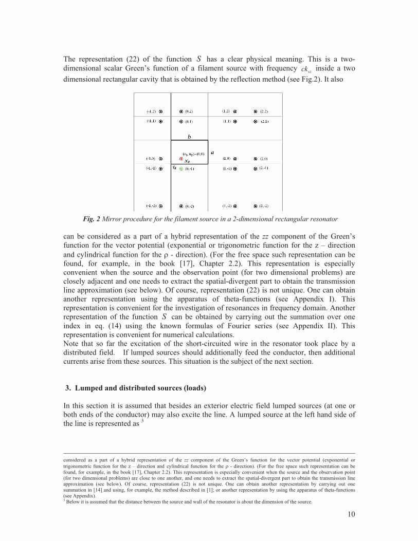
The representation (22) of the function S has a clear physical meaning. This is a two-dimensional scalar Green’s function of a filament source with frequency vzck inside a two dimensional rectangular cavity that is obtained by the reflection method (see Fig.2). It also

Fig. 2 Mirror procedure for the filament source in a 2-dimensional rectangular resonator

can be considered as a part of a hybrid representation of the zz component of the Green’s function for the vector potential (exponential or trigonometric function for the z – direction and cylindrical function for the � - direction). (For the free space such representation can be found, for example, in the book [17], Chapter 2.2). This representation is especially convenient when the source and the observation point (for two dimensional problems) are closely adjacent and one needs to extract the spatial-divergent part to obtain the transmission line approximation (see below). Of course, representation (22) is not unique. One can obtain another representation using the apparatus of theta-functions (see Appendix I). This representation is convenient for the investigation of resonances in frequency domain. Another representation of the function S can be obtained by carrying out the summation over one index in eq. (14) using the known formulas of Fourier series (see Appendix II). This representation is convenient for numerical calculations. Note that so far the excitation of the short-circuited wire in the resonator took place by a distributed field. If lumped sources should additionally feed the conductor, then additional currents arise from these sources. This situation is the subject of the next section. 3. Lumped and distributed sources (loads) In this section it is assumed that besides an exterior electric field lumped sources (at one or both ends of the conductor) may also excite the line. A lumped source at the left hand side of the line is represented as 3

considered as a part of a hybrid representation of the zz component of the Green’s function for the vector potential (exponential or trigonometric function for the z – direction and cylindrical function for the � - direction). (For the free space such representation can be found, for example, in the book [17], Chapter 2.2). This representation is especially convenient when the source and the observation point (for two dimensional problems) are close to one another, and one needs to extract the spatial-divergent part to obtain the transmission line approximation (see below). Of course, representation (22) is not unique. One can obtain another representation by carrying out one summation in [14] and using, for example, the method described in [1]; or another representation by using the apparatus of theta-functions (see Appendix). 3 Below it is assumed that the distance between the source and wall of the resonator is about the dimension of the source.

11

)(),,( 000. &�� zUzyxE llz � , 0�& (24)

with some voltage amplitude lU ( left�l ). Then one can write

��

�

�&�0

30

,,3

3)/cos()(

nnlzl hznEzU � (25)

Multiplying both sides of eq. (25) with )/~cos( 3 hzn and performing an integration over the

coordinate z from 0 to h , one finally finds for the expansion coefficients of the field 0.lzE :

)/cos( 30,0

,, 33hn

hUE l

nnlz � &� (26)

Insertion of eq. (26) into eq. (15) yields for the current )(zIl that emerges from the left � - source (for 0�& )

� �

� � 3,0

3

3

2 200

cos /:nl

l l ln z

n z hjkUI z U Y zh k k S�

�

�

�

�

� ��

� (27a)

The summation is carried out up to some maximal index 3N which is of the order &/~3 hN (this restriction corresponds to the fact that wavelengths are assumed to be larger than the dimension of the source) If the lumped source is positioned at the right hand side of the wire one similarly obtains for the current )(zIr created on the wire:

3

3

3

,0 32 2

00

( 1) cos( / )( ) : ( )

( )

nnr

r r rn vz

n z hjkUI z U Y zh k k S

� �

�

�

��

�� (27b)

If the investigated line contains lumped impedances they also can be treated as lumped sources that cause a jump in the potential (which is considered to be static for small distances) in a region ~&. In other words, they can be considered as lumped sources with unknown amplitudes (that have to be determined by the solution of a system of linear equations, see below) [20]:

)0()()0()()(),,( 111000. IZUzIZzIZzyxE llz ��'&��(&�&�� (28a)

)()()()()(),,( 22200

0. hIZUhzhIZhzhIZzyxE rrz ��'&��(&�&�� (28b)

Due to the validity of the superposition principle of electrodynamics one can represent the total exciting field 0

,tzE of the wire and the total current )(zI , respectively:

)()()()()0()( 021

0, zEhzhIZzIZzE ztz &��&�� (29)

12

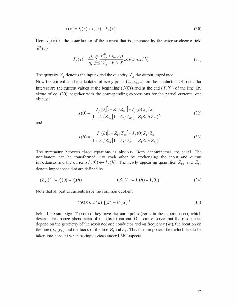
)()()()( zIzIzIzI frl � (30) Here )(zI f is the contribution of the current that is generated by the exterior electric field

)(0 zEz

)/cos()(

),()( 3

022

000,

0 3

3 hznSkk

yxEjkzIn vz

nzf

� ��

� �� (31)

The quantity 1Z denotes the input - and the quantity 2Z the output impedance. Now the current can be calculated at every point ),,( 00 zyx on the conductor. Of particular interest are the current values at the beginning ( )0(I ) and at the end ( )(hI ) of the line. By virtue of eq. (30), together with the corresponding expressions for the partial currents, one obtains:

) *) *) * 2

0121002001

012002

)/(11)(1)0(

)0(ZZZZZZZZZhIZZI

I ff

�

�� (32)

and

) *) *) * 2

0121002001

011001

)/(11)0(1)(

)(ZZZZZZZ

ZZIZZhIhI ff

�

�� (33)

The symmetry between these equations is obvious. Both denominators are equal. The nominators can be transformed into each other by exchanging the input and output impedances and the currents )()0( hII ff + . The newly appearing quantities 00Z and 01Z denote impedances that are defined by

)()0(:)( 100 hYYZ rl �� )0()(:)( 1

01 rl YhYZ �� (34) Note that all partial currents have the common quotient 122

3 ])[()/cos( �� Skkhzn vz (35) behind the sum sign. Therefore they have the same poles (zeros in the denominator), which describe resonance phenomena of the (total) current. One can observe that the resonances depend on the geometry of the resonator and conductor and on frequency ( k ), the location on the line ( 00 , yx ) and the loads of the line 1Z and 2Z . This is an important fact which has to be taken into account when testing devices under EMC aspects.

13

4. Transmission line approximation In this section it shall be shown that the lowest order approximation of the essential factor S is based on the well-known (classical) transmission line equations4. In order to derive this limit the subsequent assumptions for the validity of transmission line approximation are made: 1|||||| 00 ##�� rvzvz %��%

��, 1|| 0 ##xvz% (36)

Furthermore, it is assumed that the wire is located far enough from the other walls of resonator: 00 ,, ybax ## . Then the leading two terms ( 021 �� nn ; 0,1 21 �� nn , see red “source” and green “main mirror” in Fig.2) of the sum for S in eq. (22) are pulled out of the sum sign:

) *

��

��

"�

"��

#��

$��

"�

"��

��

��

1,0,0,

2221

)2(0

22210

)2(0

)2(0

00

1221

21

0|),),(|~(2

0|),),(|()1(

21

|))0,1(|~(|)|~(2

|))0,1(|(|)|(21),,,(

nnnn vzvz

vzvznn

vzvz

vvvz

kknnkHjkknnK

kHkHj

KKkkS

��%

��

��%��%

��

��

��

��

��

(37)

and the function ),,,( 00000 yyxxyyrxxS �� in (15) is are approximated by the natural logarithm function )/2ln( 00 rx� . Thus one obtains the known logarithmic divergence of the TL theory:

� 002ln21 rxSTL

� (38)

Using this function in all expressions for the fields, currents, admittances, etc. leads to corresponding equations for the TL theory in the resonator. This is shown in the following for all partial currents. First )(zY TL

l is considered (see eq. 27 a)

��

��

�

� � �

� �

33

3

233

3

023

3

30,

000 )/()/exp(

)/()/cos(

)/2ln(2)(

nCn

nTLl khn

hznZhjk

khnhzn

rxhjkzY

�

� (39)

Here the characteristic impedance is introduced

� 000 2ln

2rxZC

�� (40)

The function )(zY TL fulfills a differential equation of second order 4 The limiting case ��0,,, yhba (but for finite value of 0x ) leads to the well-known result for the coupling of an electromagnetic field to an infinite horizontal wire above perfectly conducting ground (see Appendix III).

14

� ��

��

��3

)/exp()( 3222

nC

TL hzjnhZ

jkzYkzdd (41)

The fact that the sum in eq. (41) can be represented as � - function yields

� )()(222 zZjkzYkzdd

C

TL �� (42)

with C

TLl

TLl Z

jkYY 200

��

This was expected since the current )()( zYUzI TL

llTLl � is generated by a � - source. Solving

the above differential equation or summing up directly eq. (39) for )(zY TLl results in [18]

)sin(

))(cos()/()/cos(21)(

122

3

32

2

3kh

zhkZj

khnhzn

kh

hZjkzY

CnC

TLl

��,

-

./0

1

��

��

��

�

�

( hz 220 )

(43) Note that the zeros in the denominator now only depend on the conductor length and frequency. In this limit the wire does not interact with the resonator. Analogously, one derives for the current that is generated by the right hand side � - source the result:

)sin()cos()(

khzk

ZjzYC

TLr �� ( hz 220 ) (44)

An interesting case of these intermediate results is the application on a line which is fed by a source at the left and terminated at the end by impedance 2Z . Then the (total) current reads

)()()()( 2 zYhIZzYUzI rll �� (45) From this it is easy to obtain the current at the beginning and at the end of the conductor

) *

)0(1)()0()0()0(

)(1)()0()0(

2

222

22

l

llllr

r

lll YZ

hYYZYUYhYZ

hYZYUI

��,

-

./0

1

�� (46a)

)0(1)()(

2 l

ll

YZhYUhI

� (46b)

for the exact result and

2

2

cos( ) sin( )(0)sin( ) cos( )

TL l c

C c

U Z j kh Z khIjZ Z j kh Z kh

��

;

)cos()sin()(

2 khZkhjZUhI

c

lTL

� (47a,b)

for the result in TL - approximation.

15

It remains to calculate the field generated current )(zI f in the TL – limit. One starts with

��

� ��

022

3

30,

3

3

)/()/cos(

)(n

nz

C

TLf khn

hznEhZ

jkzI

(48)

Inserting

zdhznzEh

Eh

zn

nz �� 0

300,0

, )/cos()(3

3

� (49)

into eq. (48) one gets

�� ),,(

022

3

330,

0

0

3

3

)/()/cos()/cos(

)()(

hzzg

n

n

C

h

zTLf

TL

khnhznhzn

hZjkzdzEzI

�

�

��

��

�

(50)

Note that the term with the sum in the integral represents the Green’s function ),,( hzzgTL � in TL approximation (for the short-circuited horizontal line). Based on known formulas (see, e.g., [18]) one can perform the summations and finally obtains

��

3��2��

��zzkzzhkzzzkzhk

khZjhzzg

C

TL

),cos())(cos(),cos())(cos(

)sin(),,( (51)

As expected, this Green’s function and current fulfill the following differential equations

��

��"�

"��

��

��

�

)()(

)(),,(

02

2

2

zEzz

Zjk

zIhzzg

kzd

dzC

TLf

TL � (52)

This concludes the investigations in the transmission line – limit. It should be emphasized that in the TL approximation there is no interference between chamber and conductor (except the boundary conditions). If, however, the frequency is in the neighborhood of an eigenfrequency of the resonator or the conditions (36) are violated, strong interaction between resonator and wire will occur. This situation is investigated in the next section. 5. Comparison of analytical and numerical results This section serves for the comparison of analytical and numerical results which are obtained by both application of the above formalism to calculate the induced current on the line as well as by numerical calculations using the program packages CONCEPT II (MoM - method) [21] and PROTHEUS (MLFMM – procedure) [22]. A lumped source at the beginning of the line was chosen as the exciting (ideal) source with U0=1 V. At the far end the line was terminated with 1, 50, 311 (see eq.(40)), and 105 Ohm (short-circuit, 50 Ohm, “matched” 2 cZ Z� , and open-circuit), respectively. For all these configurations the input impedance of the line was determined in the frequency range between 50 and 500 MHz. It is worth noting that each of these calculations took about 20 hours on a powerful parallel computer (IBM X3850 M2, calculation with 30 processors), whereas the computation time for the analytical calculation

16

was about 2 minutes. Note that the maxima of the input impedance correspond to the minima of the input current and vice versa. In addition to the exact analytical and numerical results, results were also obtained in the transmission – line limit (see eqs. in Section 4). For the numerical calculation in this limit the conductor above ground plane was chosen to connect two walls in an otherwise free space. In order to not overload this work with too many figures, only results with 4� 502Z are displayed. In Fig. 2 and Fig. 3 all occurring resonances can be identified. For example, the resonances at 160 MHz, 231 MHz, 236 MHz, 269 MHz, and 289 MHz successively correlate with the modes 321 ,,: nnnv � = 0,1,1 , 1,1,1 , 0,1,2 , 0,2,1 , and 1,1,2 of the cavity. At these frequencies the input current has maxima which arise due to the strong coupling between cavity walls and conductor.

50 100 150 200 250 300 350 400 450 5000

1000

2000

3000

4000

5000

Z 2 = 50 4

A nalytica l, w ire in resonator, exact so lution A nalytica l, w ire in resonator, T L approxim ation P R O T H EU S, w ire in resonator P R O T H EU S, w ire w ith tw o p la tes in free space

|Zin(i�

)|, 4

f, M H z

Fig. 3 Frequency dependency of the input impedance It can be recognized that the results obtained with the aid of the program package PROTHEUS agree quite well with the analytical results, whereas those calculated with CONCEPT II show amplitudes that are too high, in particular with increasing frequencies. In some cases one can also observe shifts of the resonance positions from their correct positions. Of course, in the presented spectra one also can identify the eigenresonances of the conductor itself. In Fig. 3 below they appear at 167 and 335 MHz. The positions of the resonance maxima/minima depend on the value 2Z of the impedance at the end of the conductor. Changing 2Z from very low (short – circuited) to very high (open circuit) values causes a shift of the resonance positions of 4/� . Furthermore, a reduction of

17

2 0 0 4 0 00

1 0 0 0

2 0 0 0

3 0 0 0

4 0 0 0

5 0 0 0

Z 2= 5 0 4 A n a ly tic a l P ro th e u s C o n c e p t II (N e w )

|Zin(j�

)|, 4

f , M H z

Fig. 4 Exact calculation of Zin

Fig. 5 Frequency dependencies of impedance curves for different heights the height of the line above ground (decrease of 0x ) changes the input – impedance curve in such a way that with decreasing 0x the amplitudes and the widths of the resonator peaks get smaller and, likewise, the impact (energy transfer) of the cavity on the conductor also decreases (see Fig. 5).

18

150 200 250 300 350 400 450

3

2

1

x0= 9 cmZ2=ZC=311 4

Analytical result PROTHEUS code TL approximation

|U2(j�

)/U0|

f, MHz

Fig. 6 Frequency dependence of the transfer function In addition to the input impedance also the voltage transfer function is of interest. It can be defined as a ratio of the voltage U2 across the load Z2 to the exciting voltage U1. This function defines the transfer of a signal through the wire system. For the matched load Z2=ZC in the classical transmission line theory this transfer function just reduces to a phase shift, but for the line in the resonator the results can be quite different (see Fig. 6). In Fig.6 one can see again a good agreement between analytical theory and the result of PROTHEUS code). This result can be useful, for example, for the investigation of transmission lines inside cars and aircrafts. Of course, a confirmation of the above calculations by an experiment would be desirable. First experiments have been conducted in which the input impedance ( � 0I ) was measured. A copper wire was soldered with both ends to the inner pin of male N connectors, and a network analyzer was used to measure the scattering parameters. To obtain the input impedance a one-port experiment was sufficient in which the scattering parameter 11S was measured. In a two-port measurement the current transfer ratio along the line was measured. Again a male N measurement cable was used for the connection of the network analyzer. For the connection of the end of the wire another cable had to be used. Both feedthroughs and the cables were calibrated before the experiment. The analysis of these experiments showed a good agreement with the analytical and numerical results. The measurement of the current along the line becomes more complicated since the connection to the current probe inside the resonator is complicated. The results of these experiments will be published in a separate paper (IN).

6. Conclusion. The focus of the above consideration was placed on the interaction between a current carrying conductor inside a resonator (shielded room) and the resonator itself. In order to describe this interaction the Green’s function of the resonator was used, which was derived by the mirror principle. The layout of the conductor was chosen such that it runs parallel to four of the

19

resonator walls and connects the other two. Therefore, the translation symmetry in one direction (z – direction) was retained. This fact simplified the representation of the electric field component that excited the conductor and the current distribution along the line. In both cases Fourier series for the spatial coordinate z were used. The unknown Fourier expansion coefficients ( 0

, 3nzE ,3nI ) were determined by the boundary condition for the total z-component

of the electric field on the surface of the conductor. If the wire would not be conducted parallely to four of the walls then the theory can be extended to that described in Refs. [23,24,28]. There, however, the Green’s function of the cavity had to be used. Both kinds of excitations of the conductor were permitted: with distributed sources (field – excitation) and/or with lumped sources. This is the usual case when devices in a shielded room are connected by cables. The obtained analytical and comparative numerical results demonstrate a very good agreement and a strong coupling between resonator and cable. In the calculated input impedance representations of the wire, typical resonance frequencies of the resonator show up. The energy absorption of the cable from the resonator field is particularly evident in the area of its natural frequencies. Cable conduction close to a wall will reduce this effect. Overall, it is clear that, as expected, the electromagnetic interactions strongly depend on the final operative environment of an electrical and/or electronic device. As distributed sources that excite the cable inside the resonator one may imagine electromagnetic fields which penetrate from outside through apertures into the shielded room or those which are generated from the equipment inside the resonator, like, e.g., adjacent conductors. Future research inside enclosures will include experiments and different geometries of shielded rooms. Of special interest is the cylindrical cavity which represents a basic model for a missile. Further filling of housing with equipment (like many cables and electronic components) will reduce its quality factor, and, therefore, part of the interior electromagnetic field energy is absorbed by the entire environment. As a consequence, the coupling of the exterior field to a chosen cable is also diminished. Acknowledgement The authors would like to thank Dr. D. Giri for his carefully reading of the manuscript and his fruitful comments. References [1] F.M. Tesche, M. Ianoz and T. Karlsson, EMC Analysis Method and Computational Models, Wiley, 1997. [2] “Analysis and design of ultra wideband and high-power microwave pulse interactions with electronic circuits and systems”, MURI AWARD F49620-01-1-0436, CD and http://www.ece.uic.edu/MURI-RF/. [3] S.V.Tkatchenko, G.V.Vodopianov, L.M. Martynov, "Electromagnetic field coupling to an electrically small antenna in a rectangular cavity", 13th International Zurich Symposium and Technical Exhibition on Electromagnetic Compatibility, February 16-18 1999, pp.379-384. [4] L.K. Warne, K.S.H. Lee, H.G. Hudson, W.A. Johnson, R.E. Jorgenson, and S.L. Stomach, “Statistical Properties of Linear Antenna Impedance in an Electrically Large Cavity”, IEEE Trans. Ant. Prop., vol. 51, no 5, pp.978-991, May 2003. [5] S.Tkachenko, F.Gronwald, H.-G.Krauthäuser, J. Nitsch, “High Frequency Electromagnetic Field Coupling to Small Antennas in Rectangular Resonator”, V International Congress on Electromagnetism in Advanced Applications (ICEAA), 15-19 September, 2009, pp. 74-78.

20

[6] S. Tkachenko, J. Nitsch, M. Al-Hamid, „Hochfrequente Feldeinkopplung in kleine Streuer innerhalb eines rechtwinkligen Resonators“, „Internationale Fachmesse and Kongress für Elektromagnetische Verträglichkeit“, 09.-11. März 2010, Messe Düsseldorf“, ISBN 978-3-8007-3206-7, pp.121-128. [7] S. Tkachenko, J. Nitsch, R. Vick, “HF Coupling to a Transmission Line inside a Rectangular Cavity”, in Transactions of URSI International Symposium on Electromagnetic Theory, Berlin, Germany, August 16-19, 2010. [8] N.I. Nosich, “The method of analytical regularization in wave scattering and eigenvalue problems: Foundations and review of solutions”, IEEE AP Mag. vol. 41, pp. 34–39, June 1999. [9] G. Spadacini, S. A. Pignari, and F. Marliani, “Closed-Form Transmission Line Model for Radiated Susceptibility in Metallic Enclosures”, IEEE Trans. Electromag. Compat., vol. EMC - 47, no. 4, pp. 701-708, Nov. 2005. [10] T. Konefal, J. F. Dawson, A. C. Denton, T. M. Benson, C. Christopoulos, A. C. Marvin, S. J. Porter, and D. W. P. Thomas, “Electromagnetic coupling between wires inside a rectangular cavity using multiple-mode analogous - transmission-line circuit theory,” IEEE Trans. Electromagn. Compat., vol. EMC-43, no. 3, pp. 273–281, Aug. 2001. [11] T. Konefal, J. F. Dawson, A. C. Marvin, M. P. Robinson, S.J. Porter, “A Fast Multiple Mode Intermediate Level Circuit Model for the Prediction of Shielding Effectiveness of a Rectangular Box Containing a Rectangular Aperture”, IEEE Trans. Electromagnetic Compatibility, Vol. 47, No. 4, Nov. 2005, pp. 678-691. [12] C.E. Baum, “Damping Electromagnetic Resonances in Equipment Cavities”, Interaction Notes, Note 613, 10 June 2010. [13] I. S. Shapiro, M.A. Olshanetzki, Topological Lectures for Physicists, Moscow, 1999 (in Russian) [14] D.I. Wu and D.C. Chang, “A hybrid representation of the Green’s function in an overmoded rectangular cavity,” IEEE Trans. Microw. Theory Tech., vol. MTT-36, no. 9, pp. 1334–1442, Sep. 1988. [15] S.V.Tkatchenko, G.V.Vodopianov, L.M. Martynov, "On the theory of the short - rise pulse penetration into rectangular cavities," 11th International Zurich Symposium and Technical Exhibition on Electromagnetic Compatibility, March 7 - 9, 1995, pp.513 - 518. [16] J. Nitsch, S. Tkachenko, and S. Potthast, „Pulsed Excitations of Resonators”, Interaction Notes, Note 619, 30 September 2010. [17] 5.G.T. Markov, A.F. Chaplin, Excitation of Electromagnetic Waves, Moscow, “Radio I Svjaz’ ”, 1983 (Russian) (“Vozbujshdenie Elektromagnitnuh Voln”). [18] A.P. Prudnikov, Yu.A. Brychkov, O.I. Marichev, Integrals and series. Vol.- 1: Elementary functions, Gordon & Breach, 1986. [19] A.P. Prudnikov, Yu.A. Brychkov, O.I. Marichev, Integrals and series. Vol.- 2: Special functions, Gordon & Breach, 1986. [20] M.Leontovich, M. Levin, “The theory of the excitation of oscillations in dipole antennas”, Journal Technical Physics, vol. XIV, No 9, pp. 481-506, 1944 (in Russian). [21] H.-D. Brüns, A. Freiberg and H. Singer, CONCEPT-II Manual of the Program System, TU Hamburg-Harburg, Feb. 2011 [22] D. Wulf, R. Bunger, J. Ritter and R. Beyer, Accelerated simulation of low frequency applications using PROTHEUS/MLFMA, 2nd International ITG Conference on Antennas, München, Mar. 2007, p. 240. [23] J. Nitsch, F. Gronwald, and W. Wollenberg, Radiating Nonuniform Transmission-Line Systems and the Partial Element Equivalent Circuit Method, Wiley, 2009. [24] J. Nitsch, S. Tkachenko, High-Frequency Multiconductor Transmission-Line Theory, Found. Phys. (2010) 40, 1231-1252. [25] M. Abramowitz, I.A. Stegun, Handbook of mathematical functions, Dover, 1974.

21

[26] R. Courant, D. Hilbert, Methoden der Mathematschen Physik, Springer, 1993. [27] V. Katrich, F. Novokhatskiy, “Integral Representations of the Green’s Function for the Helmholtz Equation in Parallel Plate, Rectangular Waveguide and Resonator”, Proceedings of the 11th International Conference on Mathematical Methods in Electromagnetic Theory, 11 September 2006, Kharkov, Ukraine. [28] J.B.Nitsch, S.V.Tkachenko, “Global and Modal Parameters in the Generalized Transmission Line Theory and Their Physical Meaning”, Radio Science Bulletin, 312, March 2005, pp.21-31. [29] Y. Leviatan, A.T. Adams, “The response of two-wire transmission line to incident field and voltage excitation including the effects of higher order modes”, IEEE Trans. Ant. Prop., Vol. Ap- 30, No. 5, Sept. 1982, pp.998-1003. Appendix I Representation of the function S through the Jacobi Theta – Function In this Appendix a different representation for the function S is derived demonstrating the near resonance frequency dependence in explicit form. This helps to analyze frequency shifts of the resonances caused by interaction with a transmission line. Using a simple identity for the denominator of (14)

�� jkk

kkkjkk

kjkjkjkk vvvvvvv �

(�

�� 22

2

2222

2

2222

11111

(AI.1) one can re-write equation (14) for ),,( �� kS as5

),,(),(),,( 21 �� kSSkS (AI.2)

where ��

�

��

1,21

21

)sin()sin()sin()sin(4:),(nn v

vyvyvxvx

kykykxkxk

abS ��

(AI.3a)

and

��

� �

��

1,222

2

221

)()sin()sin()sin()sin(4:),,(

nn vv

vyvyvxvx

jkkkykykxkxk

abkkS

��

(AI.3b)

The spatial dependence of the sum 2S is smooth for near coordinate values of the source point and the observation point; however, it contains all singularities in the frequency domain in explicit form. Instead of that, the sum 1S is frequency – independent, but it is singular in the space domain. Below it is demonstrated how one can extract the singularity. To do that the

5 Note that such splitting procedure is equivalent (if one multiplies the summands by the trigonometric functions

)cos()cos( zkzk vz

vz � and carries out the summation over the index n3) to a splitting of the Green’s function for the

vector potential in Lorenz gauge into the Green’s function in the Coulomb gauge and the difference between the two gauges (see, for example, [4]).

22

trigonometric functions in (AI.2) are presented as a sum of exponential functions, and an integral representation (AI.4) of the denominator in (AI.3a) is used.

� ) *��

��0

23

22

21

0

22 )/()/()/(exp)exp(1 dthnbnantdttk

k vv

, 2][][ Lt � (AI.4)

Then the summation under the integration decouples, and after rearranging the sum one obtains for S1

,,-

.

//0

1�

,,-

.

//0

1� ��

��

��

�

��

��

��

��

��

��

�

��

��

��

��

��

��

�

2

2

2

2

2

2

2

2

1

1

2

1

1

1

2

123

)()(

)()(

0

)/(1 4

1),(

n

yyna

jna

t

n

yynb

jnb

t

n

xxna

jna

t

n

xxna

jna

thnt

ee

eeeab

S

��

(AI.5)

Note that the single sums in (AI.5) can be evaluated from the Jacobi theta-function of the third kind [25] (AI.6), and one can write for S1

6:

)2cos(21),(22 2

3 kxqeqqxn

kjkx

n

k ��

��

�

��

��5 , 1#q (AI.6)

� � ) *� � ) *dtebyyebyy

eaxxeaxxeab

S

btbt

atathnt

22

2223

/3

/3

/3

/3

0

)/(1

,2/)(,2/)(

,2/)(,2/)(4

1),(

55

55��

��

��

�

��

��

(AI.7) As it was mentioned before, the sum 1S contains the spatial-divergent part. To extract this part, it is necessary to investigate the theta-functions in (AI7) for small values 0|| ��

. In this case one can show that the main contribution comes from small t values, and it is possible to change the summation by integration, for example, for the first term in the brackets (AI.7):

txx

xxjkktvx

xxna

jna

t

n

xxna

jna

te

taedkaedne

vx

vx 4

)()()(

)(

1

)(2

21

2

1

1

1

2

1��

��

��

��

��

��

�

��

��

��

��( ��

(AI.8)

After that one writes for eq. (AI.7)

6 Here the Green’s function of the two – dimensional Helmholtz equation with imaginary propagation constant (or Laplace equation for n3=0) was obtained with zero-boundary conditions for a rectangular region. For the three – dimensional Laplace equation for a rectangular region such consideration was carried out in the classical book [26]. For the three – dimensional Helmholtz equation (but with real propagation constant and without splitting (AI.2) in resonance and singular parts) for the rectangular region the Green’s function was found in [27] as integral with the product of combined theta – functions 53. The method in [27], however, requires a careful carrying out of the integration in the complex plane.

23

�,,-

.

//0

1�

,,-

.

//0

1�

�(�

��

��

��

��

� ��

��

��

� dteet

beet

aeab

SS

tyy

tyy

txx

txxn

ht

4)(

4)(

4)(

4)(

0

10||1

22222

3

41

:)',(~),(

��

��

��

�,,-

.

//0

1��

��

��

��

��

�� t

yyxxt

yyxxt

yyxxt

yyxxkt eeeee

tdt v

z 4)()(

4)()(

4)()(

4)()(

0

)(

22222222

2

41

� � )� � *

"""

�

"""

�

�

�,,-

.

//0

1

��

��

��

��

�

0,)()()()(

)()()()(ln

0,)()()()(

)()()()(

21

2222

2222

220

220

220

220

vz

vz

vz

vz

vz

vz

kyyxxyyxxyyxxyyxx

kyyxxkKyyxxkK

yyxxkKyyxxkK

(AI.9)

Here )(0 zK is a modified Bessel function of the second kind of zeroth order. To obtain the first part of eq. (AI.9), eq. (AI.10) was used (see [18]). To derive the second part of the formula it is necessary to take the limit 0�v

zk for the sum of Bessel functions.

)(2 04

0

22

arKetdt t

rta�

��

� , (AI.10)

From the integral form of eq. (AI.9) one can observe, that for coinciding values of xx �, and

yy �, this integral has a logarithmical divergence for small t which is suppressed by exponent terms when xx �, and yy �, do not coincide. Now, to regularize the exact function

),(1 �� S in (AI7) one can add and subtract 1~S from eq. (AI.7) and gets:

� � ) *6

� � ) *

)',(~

,2/)(,2/)(

,2/)(,2/)(4

1),(

14

)()(4

)()(4

)()(

4)()(

/3

/3

/3

/3

0

)/(1

222222

22

22

2223

��

55

55��

��

��

Seee

et

abebyyebyy

eaxxeaxxdteab

S

tyyxx

tyyxx

tyyxx

tyyxx

btbt

atathnt

"7

"89

,,-

.��

//0

1� ��

��

��

��

��

��

��

��

(AI.11) Note that function 1

~S of the right side in eq. (AI.11) contains a spatial logarithmical singularity (compare with eq. (22)), however, the integral part of 1S in (AI.11) is a regular function for 0|| ��

��. Now one can calculate the function

),,,( 00000 yyxxyyrxxS �� which defines the current in eq. (15). Choosing values

1xx � only in singular term, one has:

24

),,,( 00000 yyxxyyrxxS �� ),,(),,( 0020001 yxkSryxS � (AI.12)

��

� ��

1,222

02

022

00221

)()(sin)(sin4),,(

nn vv

vyvx

jkkkykxk

abkyxkS

� (AI.13)

� � ) *6

� � ) * ),,(~1,,0

,,04

1),,(

00014/

03/

3

/03

/3

0

)/(0001

20

20

20

20

22

2223

ryxSeeet

abeye

exedteab

ryxS

tyx

tx

ty

btbt

atathnt

"7

"89

//0

1

,,-

.��

� �

��

��

��

55

55

(AI.14)

� � � �

"""

�

"""

�

�

�,,-

.

//0

1

��

�

0,2ln

0,222

21),,(~

20

200

00

20

200000000

0001

vz

vz

vz

vz

vz

vz

kyxr

yx

kyxkKykKxkKrkKryxS

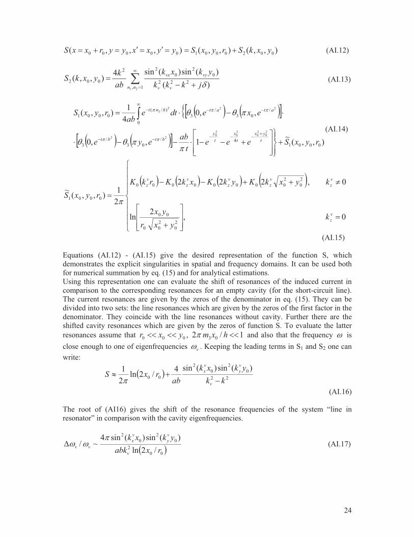
(AI.15) Equations (AI.12) - (AI.15) give the desired representation of the function S, which demonstrates the explicit singularities in spatial and frequency domains. It can be used both for numerical summation by eq. (15) and for analytical estimations. Using this representation one can evaluate the shift of resonances of the induced current in comparison to the corresponding resonances for an empty cavity (for the short-circuit line). The current resonances are given by the zeros of the denominator in eq. (15). They can be divided into two sets: the line resonances which are given by the zeros of the first factor in the denominator. They coincide with the line resonances without cavity. Further there are the shifted cavity resonances which are given by the zeros of function S. To evaluate the latter resonances assume that 000 yxr #### , 1/2 03 ##hxm and also that the frequency � is close enough to one of eigenfrequencies v� . Keeping the leading terms in S1 and S2 one can write:

� 220

20

2

00

)(sin)(sin4/2ln21

kkykxk

abrxS

v

vy

vx

�(

(AI.16) The root of (AI16) gives the shift of the resonance frequencies of the system “line in resonator” in comparison with the cavity eigenfrequencies.

� 002

02

02

/2ln)(sin)(sin4

~/rxabk

ykxk

v

vy

vx

vv

��& (AI.17)

25

Appendix II A one-dimensional sum representation of the function S In this Appendix the function S is represented as a regularized one – dimensional sum with an extracted logarithmical singularity. This representation is convenient for the numerical calculations. To do that eq.(14) is re-written as

��

�

� ��1

.2

),,,,()sin()sin(),,,(n

vyvzauxvyvyvz xxkkkSykykkkS ��

(AII.1)

Where the auxiliary function .auxS is defined by the sum

��

�

�

��

��1

~:

2222..1

2

)sin()sin(4:),,,,(n vzvyvx

vxvxvyvzauxaux

v

jkkkkxkxk

abxxkkkSS

�� %

�

��

� ��

�1

221

112

1)/~(

)/)(cos()/)/(cos(2n van

axxnaxxnb

a%

(AII.2)

Using a formula for the cosine trigonometric sum (AII.3) [18]

21

22 21

)csc())(cos()(csch))(cosh(

2)cos(

aaxaaxa

aannx

n�

789

��

� �

:�:�

�

�

(AII.3)

one can write (keep in mind an imaginary value of v%~ )

)~sinh(~)~sinh())(~sinh(2

. axxa

bS

vv

vvaux %%

%% #$�� (AII.4)

where ),max( xxx ��$ , ),min( xxx ��# . Then the equation (14) for function S becomes:

)~sinh(~)~sinh())(~sinh()sin()sin(2),,,(

12a

xxaykykb

kkSvv

vv

nvyvyvz %%

%%�� #$�

�

� � ��

(AII.5)

The series (AII.5) converges for different values of arguments �

� and �� . It diverges when

they coincide. The divergence appears during the summation for large 2n .To extract the divergent term in an explicit form the sum .auxS for large 2n is considered:

�vy

xxk

kkkvyvzaux k

eb

xxkkkSvy

vzvy

||

||.

1:),,,,(222

��

�$$

(� (AII.6)

This gives

26

��

�

�

��

1

/||22

2

)/)/(cos()/)/(cos(21~),,,(

n

bxxn

yvz

yen

byynbyynkkS

��

,-

./0

1��

� ��

��

bxxbxx

bxxbxx

eyyeeyye

/||2/||

/||2/||

))(cos(21))(cos(21ln

41

(AII.7)

During the calculation of (AII.7) a simple summation formula with complex ; ( )0Re $; is used which can be obtained by summation of geometric series and integration over parameter ; :

��

��

��

��

�

� )exp(11ln)exp(

1 ;;

n nn

(AII.8)

Adding and subtracting the infinite series (AII.7) to eq. (14) one gets

,,-

.

//0

1�

� � ��

��#$

�

��

vy

xxk

vv

vv

nvyvyvz k

eba

xxaykykb

kkSvy ||

1

1)~sinh(~

)~sinh())(~sinh(2)sin()sin(1),,,(2

%%%%��

��

,-

./0

1��

��

��

bxxbxx

bxxbxx

eyyeeyye

/||2/||

/||2/||

))(cos(21))(cos(21ln

41

(AII.9)

In this representation the logarithmic singularity is separated for closely adjacent values of the arguments. Then for the function S in the denominator of eq. (15) one can write:

�� ),,,,,( 00000 yyyyxxrxxkkS vz

,,-

.

//0

1�

� �

�

� vyvv

vv

nvy ka

xxaykb

1)~sinh(~

)~sinh())(~sinh(2)(sin1 00

10

2

2%%

%%,-

./0

1

0

0 |)sin(|ln21

ryb

(AII.10)

Equation (AII.10) gives the desired “one- dimensional sum” representation of the function S which explicitly shows the singularity in spatial coordinates. However, it contains singularities in frequency domain. Appendix III Free space limit: a,b,h � � It is of some interest to consider the limiting case a,b,h � � for the solution of the induced current (see eqs. (10),(15)) . It is expected that the result is reduced to the well-known solution for the transmission line above perfectly conducting ground excited by an arbitrary (under some restriction) electrical field. In order to approach this limit it is convenient to consider the two-dimensional filament representation of the function S (37) which - for the function in the denominator (15) - can be written as

27

�� ),,,,,( 00000 yyyyxxrxxkkS vz

��

��

"�

"��

#��

$��

1,0,0,

2221

)2(0

22210

1221

21

0|),),(|~(2

0|),),(|()1(

21),(

41

nnnn vzvz

vzvznn

vz kknnkHjkknnK

kkG��

��%

��

��

(AIII.1)

with ) *

) *"�

"��

#��

$��

0,)~2()~(

0,)2()(2),(

220

)2(00

)2(0

220000

kkxkHrkHj

kkxKrKkkG

vzvzvz

vzvvvz

%% (AIII.2)

It is assumed that the transversal dimensions of the resonator a and b , as well as the value

by ~0 tend to infinity, however, the height of the line above “ground” 0x remains finite. In the first step of calculations the length of the resonator h also remains finite. Then the term ),( vzkkG , which doesn’t depend on 0,, yba remains constant, but any term in the sum (AIII.1) containing 0,, yba in its argument tends to zero according to the asymptotic properties of cylindrical functions [25]:

)4/()2(0

2)(

��

��( zj

ze

zzH , z

ze

zzK �

��(

2)(0

(AIII.3 a,b)

Then one obtains the following equation for the term (eq.(15)) and for current � I z (eq.(10)):

��

�

�0

33

3)/cos()(

nn hznIzI ,

),()(),(4

220

000

3

3vzvz

nzn kkGkk

yxjkEI

��

�

(AIII.4 a,b)

where the terms in the Fourier series for the electrical field are given by

��h

zn

zn dzhznzyxEh

yxE0

30000,

000 )/cos(),,(),( 3

3

� (AIII.5)

If the function ),,( 00

0 zyxEz is continued for negative z, it becomes obvious that for the considered problem this function is even. As a consequence of this the summation over the index 3n of the Fourier terms ),( 00

03

yxEzn and 3nI can also be extended to negative

indices. Then it is possible to re-write the results for the cosine Fourier series as:

��

��

��3

3)/exp(~)( 3

nn hzjnIzI ,

),()(),(~4~

220

000

3

3vzvz

nzn kkGkk

yxEjkI

��

�

(AIII.4 a,b)

��

�h

hzzn dzhzjnzyxE

hyxE )/exp(),,(

21),(~

3000

000

3 (AIII.5)

28

Now assume that the length of the system tends to infinity, ��h . Then one can replace the summation by integration:

��

��

�

��

�

��

��

��

� ��z

z

kz

zjknhn

hzjnn

n

hzjnn dkeIh

heIheIzI

3

3

3

3

3

3

3

~~~)( //

(AIII.6)

hznkz /: 3� Finally one gets:

��

��

�

��

z

z

kz

zjk

zz

zz dkekkGkk

kyxjkEzI),()(

),,(2)( 220

000

�, (AIII.7)

with

��

��

� dzezyxEkyxE zjkzzz

z),,(),,( 000

000 (AIII.8)

This equation formally coincides with the well known expression for the current induced by the arbitrary exciting (incident plus reflected) field ),,( 00

0 zyxEz (see, for example [29], eq. (10), differential mode) field in the horizontal wire above perfectly conducting ground (x0 is the height of the wire). The difference is that one obtains (AIII.8) for the even field

),,(),,( 000

000 zyxEzyxE zz �� which is connected with the symmetry of our initial system.

As usual for practical calculations one has to assume small losses in the wire (a small complex part of k ) for the proper path-tracing of specific points of denominator.

Electromagnetic Field Coupling to Transmission Lines...

Documents

Transcript of Electromagnetic Field Coupling to Transmission Lines...