Electrokinetic Techniques for the Determination of ...

1. Introduction

In a porous medium the fluid flux and the electric current density are coupled, so that thestreaming potentials are generated by fluids moving through porous media and fractures.These electrokinetic phenomena are induced by the relative motion between the fluid andthe rock because of the presence of ions within water. Both steady-state and transient fluidflow can induce electrokinetics phenomena. It has been proposed to use this electrokineticcoupling to detect preferential flow paths, to detect faults and contrast in permeabilities withinthe crust, and to deduce hydraulic conductivity. This chapter proposes a comprehensivereview of the electrokinetic coupling in rocks and sediments and a comprehensive reviewof the different approaches to deduce hydraulic properties in various contexts.Electrical methods are sensitive to the fluid content because of the relative high conductivityof water compared to the one of the rock matrix. The electrical resistivity can be related tothe permeability and to the deformation, in full-saturated or in partially-saturated conditions(Doussan & Ruy, 2009; Henry et al., 2003; Jouniaux et al., 1994; 2006). The electrokineticphenomena are induced by the relative motion between the fluid and the rock matrix.In a porous medium the electric current density, linked to the ions within the fluid, iscoupled to the fluid flow (Overbeek, 1952) so that the streaming potentials are generatedby fluids moving through porous media (Jouniaux et al., 2009). The classical interpretationof the self-potential (SP) observations is that they originate from electrokinetic effect aswater flows through aquifer or fractures. Therefore some formula have been proposed topredict the permeability of porous medium or fault using the electrokinetic properties. TheSP method consists in measuring the natural electric field on the Earth’s surface. Usuallythe electric field is measured by a high-input impedance multimeter, using impolarizableelectrodes (Petiau, 2000; Petiau & Dupis, 1980) and its interpretation needs filtering techniques(Moreau et al., 1996). Moreover, for long-term observations the monitoring of the magneticfield is also needed for a good interpretation (Perrier et al., 1997). Some studies have proposedto use SP observations to infer water-table variations, to estimate hydraulic properties(Glover & Walker, 2009), and to deduce where to make a borehole for water-catchment.These studies involve surface or borehole measurements (Aubert & Atangana, 1996;Fagerlund & Heison, 2003; Finizola et al., 2003; Perrier et al., 1998; Pinettes et al., 2002), someof them have monitored self-potentials during hydraulic tests in boreholes (Darnet et al.,2006; Darnet & Marquis, 2004; Ishido et al., 1983; Maineult et al., 2008). Direct models

Electrokinetic Techniques for the Determination of Hydraulic Conductivity

Laurence Jouniaux Institut de Physique du Globe de Strasbourg,

Université de Strasbourg, Strasbourg France

16

2 Will-be-set-by-IN-TECH

(Ishido & Pritchett, 1999; Jouniaux et al., 1999; Sheffer & Oldenburg, 2007) and inverseproblems (El-kaliouby & Al-Garni, 2009; Fernandez-Martinez et al., 2010; Gibert & Pessel,2001; Gibert & Sailhac, 2008; Minsley et al., 2007; Naudet et al., 2008; Sailhac et al., 2004;Saracco et al., 2004) have been developed to locate the source of self-potential. Because ofsimilarity between the electrical potential with pressure behavior, it has been proposed alsoto use SP measurements as an electrical flow-meter (Pezard et al., 2009). However, inferringa firm link between SP intensity and water flux is still difficult. Recent modeling has shownthat SP observations could detect at distance the propagation of a water front in a reservoir(Saunders et al., 2008).We distinguish 1) The steady-state and passive observations which consist in measuringthe electrical self-potential (SP). 2) The transient and active observations which consist inmeasuring the electrical potential induced by the propagation of a seismic wave. Theseobservations are called seismo-electric conversion. The reverse can also be observed:the detection of a seismic wave induced by injection of electrical current and is calledelectro-seismic conversion.

2. Streaming potential coefficient in rocks and sediments

2.1 Theoretical backgroundThe fluid flow in porous media or in fractures can induce electrokinetic effect because of thepresence of ions within the fluid which can induce electric currents when water flows. Thegeneral equation coupling the different flows is,

Ji =N

∑j=1LijXj (1)

which links the forces Xj to the macroscopic fluxes Ji, through transport coupling coefficientsLij (Onsager, 1931).When dealing with the coupling between the hydraulic flow and the electric flow, assuming aconstant temperature, and no concentration gradients, the electric current density Je [A.m−2]and the flow of fluid Jf [m.s−1] can be written as the following coupled equation:

Je = −σ0∇V −Lek∇P. (2)

Jf = −Lek∇V − k0

η f∇P. (3)

where P is the pressure that drives the flow [Pa], V is the electrical potential [V], σ0 is the bulkelectrical conductivity [S.m−1], k0 the bulk permeability [m2], η f the dynamic viscosity of thefluid [Pa.s], Lek the electrokinetic coupling [A Pa−1 m−1]. Thus the first term in equation 2 isthe Ohm’s law and the second term in equation 3 is the Darcy’s law. The coupling coefficientsmust satisfy the Onsager’s reciprocal relation in the steady state: the coupling coefficient istherefore the same in equation 2 and equation 3. This reciprocity has been verified on porousmaterials (Auriault & Strzelecki, 1981; Miller, 1960) and on natural materials (Beddiar et al.,2002).The streaming potential coefficient Cs0 [V.Pa−1] is defined when the electric current density Jeis zero, leading to

308 Hydraulic Conductivity – Issues, Determination and Applications

Electrokinetic Techniques for the Determination of Hydraulic Conductivity 3

ΔVΔP

= −Lekσ0

= Cs0 (4)

This coefficient can be measured by applying a driving pore pressure ΔP to a porous mediumand by detecting the induced electric potential difference ΔV. The driving pore pressureinduces a streaming current (second term in eq. 2) which is balanced by the conduction current(first term in eq.2) which leads to the electric potential difference ΔV that can be measured.We detail here what we know about this streaming potential coefficient (SPC) on sands androcks because we will see that it can be used with the electro-osmosis coefficient to deducethe permeability. In the case of a unidirectional flow through a cylindrical saturated porouscapillary, this coefficient can be expressed as (Jouniaux et al., 2000; Jouniaux & Pozzi, 1995b):

Cs0 =ε f ζ

η f σe f f(5)

with the fluid electrical permittivity ε f [F.m−1], the effective electrical conductivity σe f f

[S.m−1] defined as σe f f = Fσ0 with F the formation factor and σ0 the rock conductivity whichcan include a surface conductivity. The potential ζ [V] is the zeta potential described as theelectrical potential inside the EDL at the slipping plane or shear plane (i.e., the potential withinthe double-layer at the zero-velocity surface). Minerals forming the rock develop an electricdouble-layer when in contact with an electrolyte, usually resulting from a negatively chargedmineral surface. An electric field is created perpendicular to the surface of the mineral whichattracts counterions (usually cations) and repulses anions in the vicinity of the pore matrixinterface. The electric double layer (Fig. 1) is made up of the Stern layer, where cations areadsorbed on the surface, and the Gouy diffuse layer, where the number of counterions exceedsthe number of anions (Adamson, 1976; Davis et al., 1978; Hunter, 1981). The streaming currentis due to the motion of the diffuse layer induced by a fluid pressure difference along theinterface. This streaming current is then balanced by the conduction current, leading tothe streaming potential. When the surface conductivity can be neglected compared to thefluid conductivity Fσ0 = σf and the streaming coefficient is described by the well-knownHelmholtz-Smoluchowski equation (Dukhin & Derjaguin, 1974):

Cs0 =ε f ζ

η f σf(6)

The assumptions are a laminar fluid flow and identical hydraulic and electric tortuosity.The influencing parameters on this streaming potential coefficient are therefore the dielectricconstant of the fluid, the viscosity of the fluid, the fluid conductivity and the zeta potential,itself depending on rock, fluid composition, and pH (Guichet et al., 2006; Ishido & Mizutani,1981; Jaafar et al., 2009; Jouniaux et al., 2000; Jouniaux & Pozzi, 1995a; Lorne et al., 1999a;Vinogradov et al., 2010). There exists a pH for which the zeta potential is zero: this is theisoelectric point and pH is called pHIEP (Davis & Kent, 1990; Sposito, 1989). At a given pHthe most influencing parameter is the fluid conductivity (Fig.2). When collecting data fromliterature on sands and sandstones we can propose that Cs0 = −1.2 x 10−8σ−1

f which leadsto a zeta potential equal to −17 mV assuming eq. 6 and that zeta potential and dielectricconstant do not depend on fluid conductivity. These assumptions are not exact, but the valueof zeta is needed for numerous modellings which usually assume the dielectric constantnot dependent on the fluid conductivity. Therefore an average value of −17 mV for such

309Electrokinetic Techniques for the Determination of Hydraulic Conductivity


modellings is rather exact, at least for medium with no clay nor calcite. Another formulais often used (Pride & Morgan, 1991) based on quartz minerals rather than on sands andsandstones, which may be less appropriate for field applications. When the medium is notfully saturated Perrier & Morat (2000) suggested a model in which the streaming potentialcoefficient is dependent on a relative permeability model kr.

C(Sw) = Cs0kr

Swn (7)

assuming that the relative electrical conductivity is equal to Snw. The parameter n is the

Archie saturation exponent (Archie, 1942). This exponent has been observed to be about 2for consolidated rocks and in the range 1.3 < n < 2 for coarse-texture sand (Guichet et al.,2003; Lesmes & Friedman, 2005; Schön, 1996). Note that the use of Archie’s law is valid inthe absence of surface electrical conductivity. Recently Allègre et al. (2010) (and Allègre et al.(2011)) proposed original streaming potential measurements performed during a drainageexperiment and measured the first continuous recordings of the streaming potential coefficientas a function of water saturation. These authors observed that the streaming potentialcoefficient exhibits two different behaviours as the water saturation decreases. Values ofCs0 first increase for decreasing saturation in the range 0.55 − 0.8 < Sw < 1, and thendecrease from Sw = 0.55 − 0.8 to residual water saturation. This behaviour was neverreported before and still needs further interpretation. Jackson (2010) used a bundle capillarymodel to compute the streaming potential coefficent as a function of water-saturation. Heshowed that the behaviour of the SPC depends on the capillary size distribution, the wettingbehaviour of the capillaries, and whether we invoke the thin or thick electrical double layerassumption. Depending upon the chosen value of the saturation exponent and the irreductiblewater-saturation, the relative SPC may increase at partial saturation, before decreasing tozero at the irreductible saturation. Up to now permeability predictions using electrokinetictechniques use theoretical developments in full saturated conditions.Similarly the electro-osmosis coefficient is defined when the flow of fluid Jf is zero, leading to

ΔPΔV

= −Lekη

k0= Ce0 (8)

This coefficient can be measured by applying an electric potential difference ΔV and bydetecting the induced electro-osmotic flow [m.s−1] corresponding to the first term of equation3, by controlling the hydraulic gradient, usually maintaining identical water heads. Assumingthe Helmholtz-Smoluchowski equation (eq. 6) the electro-osmosis coefficient can be writtenas:

Ce0 =εζ

k0F(9)

and then depends also on pH (Beddiar et al., 2005) through the zeta potential.Since the permeability and the formation factor are not independent, but can be related byk0 = CR2/F (Paterson, 1983) with C a geometrical constant usually in the range 0.3-0.5 and Rthe hydraulic radius, the electro-osmosis coefficient can be written as:

Ce0 =εζ

CR2 (10)



As we can see from this section, the streaming potential coefficient and the electro-osmosiscoefficient are directly proportional to the zeta potential, which can not be directly measuredand which is difficult to model at a rock-water interface. Therfore the zeta potential isusually deduced from streaming potential measurements. Moreover the streaming potentialcoefficient is inversely proportional to the fluid conductivity, whereas the electro-osmosiscoefficient is inversely proportional to the hydraulic radius.

2.2 Permeability predictionThese electrokinetic properties have been used to predict the permeability. Li et al. (1995)defined an electrokinetic permeability ke by the following relation:

ke = ησrCs0

Ce0(11)

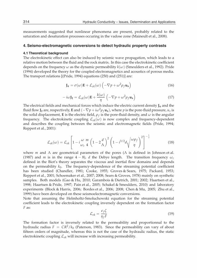
with σr the rock conductivity (measured when Jf is zero).These authors verified on 12 samples of sandstones, limestones and fused glass beads that theelectrokinetic permeability ke successfully predicts the rock permeability kr (measured whenJe is zero) over a range of about four decades from 10−15 to 10−11 m2. Pengra et al. (1999)verified also this relation on eight samples of sandstone and limestone, and four fused glassbeads, in the permeability range 10−15 to 10−11 m2 (Fig. 3). This approach has been used topropose the permeability measurement (Wong, 1995) within boreholes (Fig. 4). The advantagewas that we only needed to apply or to measure the pressure and the electric field.A simplest way to measure the permeability in borehole, was performed using only thestreaming potential coefficient (eq. 4). Although this coefficient does not depend directlyon permeability, Hunt & Worthington (2000) showed that the borehole streaming potentialresponse could detect fractures and cracks. A pressure pulse is generated by a nylonblock which displaces water as it moves upwards (Fig. 5). This mechanical system avoidsspurious electrical noise induced by electro-mechanical systems. The electrode response isnormalized to the peak pressure recorded by the hydrophone. The authors showed that themaximum electrical signal was clearly associated with the highest fracture density and thewidest aperture (few cm). The recorded amplitudes were in the range 4x10−7 to 1.5x10−6

V/Pa. It was proposed that the fluid flow in the cracks causing the streaming potential waspredominantly caused by the seismic wave within the rock that distorts crack aperture as itpasses, rather than by the source directly forcing fluid into cracks. In this case the permeabilitydependence of the streaming potential coefficient may be linked to the indirect effect of surfaceconductivity which may not be negligeable: the effective conductivity can decrease withincreasing permeability, leading to an increase in the streaming potential coefficient (eq. 5)(Jouniaux & Pozzi, 1995a).Recently, Glover et al. (2006) proposed a new prediction for the permeability by comparing anelectrical model derived from the effective medium theory to an electrical model for granularmedium. These authors derived the RGPZ model defined as:

kRGPZ =d2φ3m

4am2 (12)

where φ is the porosity, m the cementation exponent from the Archie’s law, a is a parameterthought to be equal to 8/3 for samples composed of quasi-spherical grains, and d is therelevant grain size. They showed that the relevant grain size is the geometric mean, whichcan be deduced from Mercury Injection Capillary Pressure (MICP). The relevant grain size



can also be inferred from borehole NMR data, and then must be deduced from an empiricalprocedure relating grain size to the T2 relaxation time. This new model was shown to matchdata over 348 samples over a 500 m thick sand-shale succession in the North Sea. Since theporosity can also be derived from NMR data, the advantage of this approach is to provide alog of permeability along the studied borehole, at the scale which is investigated by the NMRtool.

3. Fault and hydraulic fracturing

3.1 Permeability prediction within faultIt has also been proposed to deduce the permeability of the Nojima fault (Japan) using theself-potential observations in surface when water is injected into a well of 1800 m depth(Murakami et al., 2001). Water flow is induced at about 1600 m depth when crossing thefracture zone, and the change in voltage in the aquifer is conducted to the whole part ofthe well through the iron casing pipe (Fig. 6). Therefore the electrokinetic source occuring atdepth can be detected at the surface. Self-potential variations of 10-35 mV in response to waterpressure of 35-38x105 Pa were observed. The magnitude of self-potential variations decreaseswith increasing distance from the injection well. An amplitude of −20 mV was detectednear the well, about −10 mV at 40 m, and within the noise at one hundred meters. Theelectrokinetic source is the dragging current expressed by the second term in eq. 2. Assumingthe Helmholtz-Smoluchowski equation (eq. 6) and the Darcy’s law (second term in eq. 3), andusing the definition of the formation factor F, we can write the dragging current:

Jedragg = − ε f ζ

FkJf (13)

This dragging current is balanced by the conduction current (the first term in eq. 2).Assuming a line source model with L the length of the casing pipe, the potential difference ΔVbetween two electrodes at the surface is related to the total conduction current Icond−tot [A] by(Murakami et al., 2001):

ΔV =Icond−tot2πσr L

log(a/b) (14)

where a and b are the distances from the borehole to the electrodes. Then the permeability ofthe fault is deduced by:

k f ault = −ε f ζ

F

Q f−tot

Icond−tot(15)

The total conduction current Icond−tot is deduced from surface potential measurements ΔV(eq. 14). The total water injection (usually several liters/min) provides the value of Q f−tot

[m3s−1]. The formation factor F of the fault can be deduced from resistivity well-loggingassuming Archie’s law and knowing the fluid conductivity. The value of zeta potential hasto be deduced from laboratory experiments published in the literature, possibly using figure2. Murakami et al. (2001) deduced that the permeability of the fault was higher at the endof the water injection than at the beginning. Assumming different hypotheses for the zetapotential to −1 to −10 mV they deduced a permeability in the range 10−16 to 10−15 m2. Thechemical properties of the injected water is important since it can decrease dramatically thezeta potential if species such as Ca2+ or Al3+ are present in high quantity. The advantage ofthis method is to be able to deduce the permeability at depth of the fault.



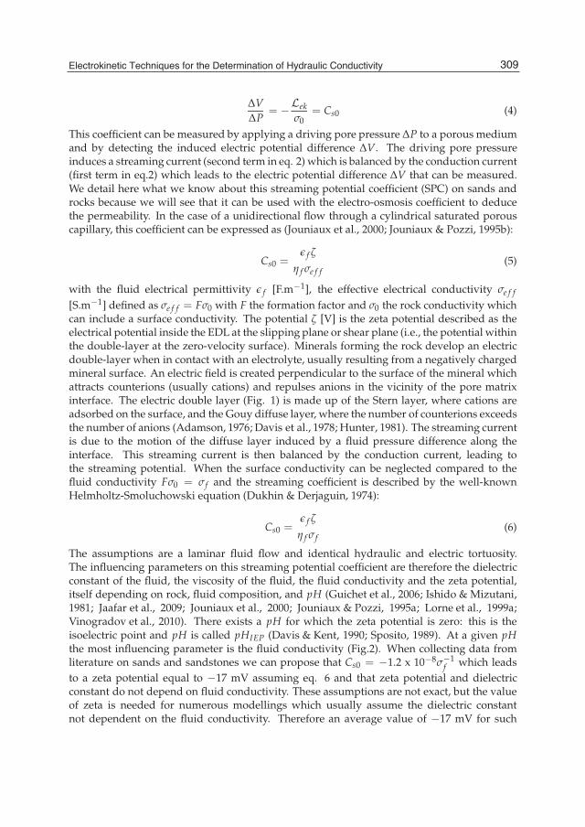
3.2 Self-potentiels related to hydraulic fracturingSince fluid flow can create streaming potentials, the hydraulic fracturing can induce streamingpotentials as the fracture propagates, if the fracture remains fullfilled with water.Laboratory experiments on hydraulic fracturing on granite samples showed that thestreaming potential varies linearly with the injection pressure (Moore & Glaser, 2007).However the SPC increases in an exponential trend when approaching the breakdownpressure. Since the permeability also shows an exponential increase with injection pressure,the authors concluded that the SPC is varying as k1.5. The explanation was not an effect due tothe surface conductivity, but a difference in the hydraulic tortuosity (David, 1993) and electrictortuosity (as suggested by Lorne et al. (1999b)) induced by dilatancy of microcracks.The streaming potential induced by an advancing crack has been modeled by Cuevas et al.(2009). The authors modeled the streaming electric current density by defining a source-timefunction from the pressure profile in the propagating direction of the opening crack. Thestreaming electric current is maximum at the tip of the fracture and decays exponentiallyin front of the tip. The decay constant linearly increases with the propagation speed of thefracture. As the fractures progresses, the streaming potential observed at a distant pointresults from a superposition of delayed sources arising at the position of the advancing fluidfront. The results show that the energy is focused in the vicinity of the advancing fracture’stip, however a tail can also be distinguished as the source behind the tip does not vanishinstantaneously. Cuevas et al. (2009) could model the streaming electrical spike recorded byMoore & Glaser (2007) during hydraulic fracturing by modeling the propagation of two cracksand adjusting the propagation velocity, the direction of propagation and the initial fracturevolume. The authors concluded that direct information of the hydraulic fracture propagationcan be provided by measuring the electrical field at distant.Hydraulic stimulation is often used to stimulate fluid flow in geothermal reservoirs. Surfaceelectrical potentials were measured when water was injected (during about 7 days) ingranite at 5 km depth at the Soultz Hot Dry Rock site (France) (Marquis et al., 2002). Ananomalous potential of about 5 mV was interpreted as an electrokinetic effect a depthand measured at the surface because of the conductive well casing. The question of theexact origin between electrokinetic and electrochemical (Maineult, Bernabé & Ackerer, 2006;Maineult, Jouniaux & Bernabé, 2006) effects was raised by Darnet et al. (2004). Finally ithas been shown that whatever the injection rate was, the electrochemical contribution wasalmost negligeable (Maineult, Darnet & Marquis, 2006): the SP anomaly was mainly relatedto the temperature contrast between the in-situ brine and the injected fresh water only atthe earliest stage of injection, and was essentially related to water-flows afterwards. Furtherinvestigations showed that a slow SP decay is observed after shut-in : its was interpretedas related to large fluid-flow persisting after the end of stimulation and correlated to themicroseismic activity (Darnet et al., 2006). The fluid flow was not detected on hydraulicdata because it took place in a zone hydraulically disconnected from the openhole. Theauthors concluded that the SP observations could monitor the fluid flow at the reservoirscale and revealed that the fluid flow plays a major role in the mechanical response ofthe reservoir to hydraulic stimulation. Another field experiment was performed withperiodic pumping tests (injection/production) in a borehole penetrating a sandy aquifer(Maineult et al., 2008). The attenuation of SP amplitude with distance was roughly similarto the pressure attenuation. Therefore the authors proposed that hydraulic diffusivity couldbe inferred from SP observations. Moreover the comparaison between surface and borehole



measurements suggested that nonlinear phenomena are present, probably related to thesaturation and desaturation processes occuring in the vadose zone (Maineult et al., 2008).

4. Seismo-electromagnetic conversions to detect hydraulic property contrasts

4.1 Theoretical backgroundThe electrokinetic effect can also be induced by seismic wave propagation, which leads to arelative motion between the fluid and the rock matrix. In this case the electrokinetic coefficientdepends on the frequency ω as the dynamic permeability k(ω) (Smeulders et al., 1992). Pride(1994) developed the theory for the coupled electromagnetics and acoustics of porous media.The transport relations [(Pride, 1994) equations (250) and (251)] are:

Je = σ(ω)E + Lek(ω)(−∇p + ω2ρ f us

)(16)

− iωJf = Lek(ω)E +k(ω)

η

(−∇p + ω2ρ f us

)(17)

The electrical fields and mechanical forces which induce the electric current density Je and thefluid flow Jf are, respectively, E and (−∇p+ iω2ρ f us), where p is the pore-fluid pressure, us isthe solid displacement, E is the electric field, ρ f is the pore-fluid density, and ω is the angularfrequency. The electrokinetic coupling Lek(ω) is now complex and frequency-dependentand describes the coupling between the seismic and electromagnetic fields (Pride, 1994;Reppert et al., 2001):

Lek(ω) = Lek

⎡⎣1− i

ω

ωc

m4

(1− 2

dΛ

)2(

1− i3/2d

√ωρ f

η

)2⎤⎦− 1

2

(18)

where m and Λ are geometrical parameters of the pores (Λ is defined in Johnson et al.(1987) and m is in the range 4 − 8), d the Debye length. The transition frequency ωcdefined in the Biot’s theory separates the viscous and inertial flow domains and dependson the permeability k0. The frequency-dependence of the streaming potential coefficienthas been studied (Chandler, 1981; Cooke, 1955; Groves & Sears, 1975; Packard, 1953;Reppert et al., 2001; Schoemaker et al., 2007; 2008; Sears & Groves, 1978) mainly on syntheticsamples. Both models (Gao & Hu, 2010; Garambois & Dietrich, 2001; 2002; Haartsen et al.,1998; Haartsen & Pride, 1997; Pain et al., 2005; Schakel & Smeulders, 2010) and laboratoryexperiments (Block & Harris, 2006; Bordes et al., 2006; 2008; Chen & Mu, 2005; Zhu et al.,1999) have been developed on these seismoelectromagnetic conversions.Note that assuming the Helmholtz-Smoluchowski equation for the streaming potentialcoefficient leads to the electrokinetic coupling inversely dependent on the formation factorF as:

Lek =ε f ζ

η f F(19)

The formation factor is inversely related to the permeability and proportionnal to thehydraulic radius F = CR2/k0 (Paterson, 1983). Since the permeability can vary of aboutfifteen orders of magnitude, whereas this is not the case of the hydraulic radius, the staticelectrokinetic coupling Lek will increase with increasing permeability.



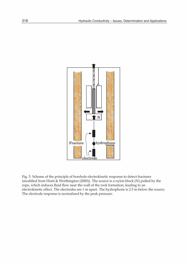
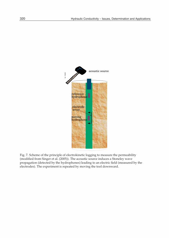
4.2 Detection of permeability contrastsTwo kinds of mechanical to electromagnetic conversions exist: 1) The electrokinetic signalwhich travels with the acoustic wave; 2) The interfacial conversion occuring at contrasts ofphysical properties such as permeability.The first kind of conversion has been used to show that a reliable permeability log canbe derived from electrokinetic measurements (Singer et al., 2005), using an acoustic sourcewithin a borehole (Fig. 7). Singer et al. (2005) showed by a finite element model and bylaboratory experiments that the normalized coefficient defined by the electric field dividedby the pressure depends [V Pa−1 m−1] on the permeability. This coefficient is coherent withthe electrokinetic coefficient Lek (eq. 19) per unit of conductance [S] and then should increasewith increasing permeability. At low permeability the oscillating source will induce a largersolid displacement because the fluid is not easily displaced. However the relative movementbetween solid and fluid is limited, leading to a decrease of the electric field even if pressureincreases, so that this normalized coefficient is decreased. The investigated depth of such apermeability is of the order of centimeters. The source was a short steel tube near the top ofthe borehole and hit on top with a hammer. The main wave propagation is a Stoneley wavewhich induces the electric field. The logging tool is moved step-by-step within the borehole(Fig. 7). This model showed that the normalized coefficient could detect a 0.5 m-thick bed ofpermeability 10−13m2 within a formation of permeability 10−15 m2. The measured amplitudeof the normalized coefficient on sandstones is in the range 1.6x10−7 to 2.5x10−6 [V Pa−1 m−1]increasing with increasing permeabilities from 6.2 10−15 m2 to 2.2x10−12 m2.The second kind of conversion can be used to detect contrasts in permeability in the crust.The seismic source induces a seismic wave propagation downward up to the interface (Fig.8). Because of the difference in the physical properties there is a charge inbalance that causesa charge separation on both sides of the interface. This acts as en electric dipole which emitsan electromagnetic wave that travels with the speed of the light in the medium and that canbe detected at the surface (Fig. 9). The velocity of the seismic wave propagation is deduced bysurface measurements of the soil velocity. Then the depth of the interface can be deduced bypicking the time arrival of the electromagnetic wave. Usually the seismoelectric signals showlow amplitude from 100 μV to mV. Then signal processing needs filtering techniques such asButler & Russell (1993). The advantage of this method is to detect the contrasts of permeabilityat depth from few meters to few hundreds of meters (Dupuis & Butler, 2006; Dupuis et al.,2007; Dupuis et al., 2009; Haines, Guitton & Biondi, 2007; Haines, Pride, Klemperer & Biondi,2007; Strahser et al., 2007; 2011; Thompson et al., 2005).

5. Limitations of this technique

The limitations of this technique arise from the low amplitude of the electrical signal. It needsgood pre-amplifiers to be able to detect the signals. Then it needs an adapted signal processingto remove the anthropic noise, and further filtering techniques to extract the expected signalfrom the remaining records. The interpretation of self-potential observations may not be easyif the signals are induced not only by the electrokinetic effect, but also by a thermoelectriceffect, and by an electrochemical effect. The interpretation of the seismo-electric conversionmay not be easy if the contrast in the permeability is not high enough.



Fig. 1. Electric double layer, courtesy of P.W.J. Glover (Glover & Jackson, 2010). The solidmineral presented is the case of silica. At pH above the isoelectric point the cations areadsorbed within the Stern layer; there is an excess of cations in the diffuse layer. The zetapotential is defined at the shear plane. The fluid flow creates a streaming current which isbalanced by the conduction current, leading to the streaming potential.

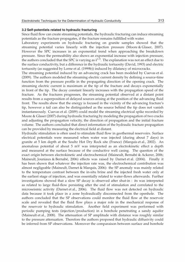
Fig. 2. Streaming potential coefficient from data collected (in absolute value) on sands andsandstones at pH 7-8 (when available) from Ahmad (1964); Guichet et al. (2006; 2003);Ishido & Mizutani (1981); Jaafar et al. (2009); Jouniaux & Pozzi (1997); Li et al. (1995);Lorne et al. (1999a); Pengra et al. (1999); Perrier & Froidefond (2003). The regression (blackline) leads to Cs0 = −1.2 x 10−8σ−1

f . A zeta potential of −17 mV can be inferred from thesecollected data (from Allègre et al. (2010)).



Fig. 3. Comparison between the permeability k and the electrokinetic permeability ke. Thesolid line is ke=k (modified from Pengra et al. (1999)).

Fig. 4. In-situ permeability measurement (from Wong (1995)) from streaming potential andelectro-osmosis measurements using eq. 11. For the streaming potential measurement: anoscillating presure is applied by electromechanical transducer (22) to the rock formation (20)through fluid chamber (21) with valve (42) open. The pressure differential in the rockbetween fluid chamber (21) and (21’) is measured by a pressure sensor (25) and the inducedvoltage difference is measured by the voltage electrodes (32) and (32’). For theelectro-osmosis measurements the valve (42) is closed, the pressure difference induced whena current is passed through the rock (by current electrodes 29 and 29’) is measured bypressure sensor (25).



Fig. 5. Scheme of the principle of borehole electrokinetic response to detect fractures(modified from Hunt & Worthington (2000)). The source is a nylon block (N) pulled by therope, which induces fluid flow near the wall of the rock formation, leading to anelectrokinetic effect. The electrodes are 1 m apart. The hydrophone is 2.5 m below the source.The electrode response is normalized by the peak pressure.



Fig. 6. Measurement of the permeability of the Nojima fault (modified from Murakami et al.(2001)). The water injection inside the borehole of 1800 m depth crosses the fault inducing anelectrokinetic source at depth within the fault. The conduction current is conducted by theiron pipe up to the surface. The difference of potential V is measured by electrodes on thesurface. The permeability is deduced from eq. 15



Fig. 7. Scheme of the principle of electrokinetic logging to measure the permeability(modified from Singer et al. (2005)). The acoustic source induces a Stoneley wavepropagation (detected by the hydrophones) leading to an electric field (measured by theelectrodes). The experiment is repeated by moving the tool downward.



Fig. 8. The seismic waves propagates up to the interface where an electric dipole is generatedbecause of the contrast in permeability. This electromagnetic wave can be detected at thesurface by measuring the difference of the electrical potential V between electrodes. Pickingthe time arrival allows to know the depth of the interface.



Fig. 9. Model of the seimoelectric response to a hammer strike on the surface at position zero(from Haines (2004)). The seismoelectric signal is shown as measured at the surface along aline centered on the seismic source. The interfacial signal is related to a contrast betweenproperties of the media, such as the permeability.

6. Conclusion

The electrokinetic properties can be used to deduce permeability in the crust, possibly atdepth, within fault, and along boreholes. Some conditions are needed to be able to useelectrokinetic coupling to infer hydraulic properties. The electrical noise can prevent beingable to detect small electric potentials, even using appropriate filtering techniques. Whenpossible, the joint inversion with other observations can improve parameters such as electricalconductivity. The seismoelectric method could provide deeper investigations when usingstronger seismic sources.

7. Acknowledgements

This work was supported by the French National Scientific Center (CNRS), byANR-TRANSEK, and by REALISE the "Alsace Region Research Network in EnvironmentalSciences in Engineering" and the Alsace Region.

8. References

Adamson, A. W. (1976). Physical chemistry of surfaces, John Wiley and sons, New York.Ahmad, M. (1964). A laboratory study of streaming potentials, Geophys. Prospect. XII: 49–64.Allègre, V., Jouniaux, L., Lehmann, F. & Sailhac, P. (2010). Streaming Potential dependence on

water-content in fontainebleau sand, Geophys. J. Int. 182: 1248–1266.Allègre, V., Jouniaux, L., Lehmann, F. & Sailhac, P. (2011). Reply to the comment by A. Revil

and N. Linde on: "Streaming potential dependence on water-content in fontainebleausand" by Allègre et al., Geophys. J. Int. 186: 115–117.

Archie, G. E. (1942). The electrical resistivity log as an aid in determining some reservoircharacteristics, Trans. Am. Inst. Min. Metall. Pet. Eng. (146): 54–62.



Aubert, M. & Atangana, Q. Y. (1996). Self-potential method in hydrogeological exploration ofvolcanic areas, Ground Water 34: 1010–1016.

Auriault, J. & Strzelecki, T. (1981). On the electro-osmotic flow in saturated porous media, Int.J. Engrg. Sci. 19: 915–928.

Beddiar, K., Berthaud, Y. & Dupas, A. (2002). Experimental verification of the onsager’sreciprocal relations for electro-osmosis and electro-filtration phenomena on asaturated clay, C. R. Mécanique 330: 893–898.

Beddiar, K., Fen-Chong, T., Dupas, A., Berthaud, Y. & Dangla, P. (2005). Role of ph inelectro-osmosis: Experimental study on nacl-water saturated kaolinite, Transport inPorous media 61: 93–107.

Block, G. I. & Harris, J. G. (2006). Conductivity dependence of seismoelectric wave phenomenain fluid-saturated sediments, J. Geophys. Res. 111: B01304.

Bordes, C., Jouniaux, L., Dietrich, M., Pozzi, J.-P. & Garambois, S. (2006). First laboratorymeasurements of seismo-magnetic conversions in fluid-filled Fontainebleau sand,Geophys. Res. Lett. 33: L01302.

Bordes, C., Jouniaux, L., Garambois, S., Dietrich, M., Pozzi, J.-P. & Gaffet, S. (2008). Evidence ofthe theoretically predicted seismo-magnetic conversion, Geophys. J. Int. 174: 489–504.

Butler, K. E. & Russell, R. D. (1993). Substraction of powerline harmonics from geophysicalrecords, Geophysics 58: 898–903.

Chandler, R. (1981). Transient streaming potential measurements on fluid-saturated porousstructures: An experimental verification of Biot’s slow wave in the quasi-static limit,J. Acoust. Soc. Am. 70: 116–121.

Chen, B. & Mu, Y. (2005). Experimental studies of seismoelectric effects in fluid-saturatedporous media, J. Geophys. Eng. 2: 222–230.

Cooke, C. E. (1955). Study of electrokinetic effects using sinusoidal pressure and voltage, J.Chem. Phys. (23): 2299–2303.

Cuevas, N., Moore, J. & Glaser, S. (2009). Electrokinetic coupling in hydraulic fracturepropagation, SEG Technical Program Expanded Abstracts 28: 1721–1725.

Darnet, M., G.Marquis & Sailhac, P. (2006). Hydraulic stimulation of geothermalreservoirs:fluid flow, electric potential and microseismicity relationships, Geophys. J.Int. 166: 438–444.

Darnet, M., Maineult, A. & Marquis, G. (2004). On the origins of self-potential (sp) anomaliesinduced by water injections into geothermal reservoirs, Geophys. Res. Lett. 31: L19609.

Darnet, M. & Marquis, G. (2004). Modelling streaming potential (sp) signals induced by watermovement in the vadose zone, J. Hydrol. 285: 114–124.

David, C. (1993). Geometry of flow paths for fluid transport in rocks, J. Geophys. Res.98: 12267–12278.

Davis, J. A., James, R. O. & Leckie, J. (1978). Surface ionization and complexation at theoxide/water interface, J. Colloid Interface Sci. 63: 480–499.

Davis, J. & Kent, D. (1990). Surface complexation modeling in aqueous geochemistry, in MineralWater Interface Geochemistry, M.F. Hochella and A.F. White, Mineralogical Society ofAmerica.

Doussan, C. & Ruy, S. (2009). Prediction of unsaturated soil hydraulic conductivity withelectrical conductivity, Water Resources Res. 45: W10408.

Dukhin, S. S. & Derjaguin, B. V. (1974). Surface and Colloid Science, edited by E. Matijevic, JohnWiley and sons, New York.



Dupuis, J. C. & Butler, K. E. (2006). Vertical seismoelectric profiling in a borehole penetratingglaciofluvial sediments, Geophys. Res. Lett. 33.

Dupuis, J. C., Butler, K. E. & Kepic, A. W. (2007). Seismoelectric imaging of the vadose zoneof a sand aquifer, Geophysics 72: A81–A85.

Dupuis, J. C., Butler, K. E., Kepic, A. W. & Harris, B. D. (2009). Anatomy of a seismoelectricconversion: Measurements and conceptual modeling in boreholes penetrating asandy aquifer, J. Geophys. Res. Solid Earth 114(B13): B10306.

El-kaliouby, H. & Al-Garni, M. (2009). Inversion of self-potential anomalies caused by 2dinclined sheets using neural networks, J. Geophys. Eng. 6: 29–34.

Fagerlund, F. & Heison, G. (2003). Detecting subsurface grounwater flow in fractured rockusing self-potential (sp) methods, Environmental Geology 43: 782–794.

Fernandez-Martinez, J., Garcia-Gonzalo, E. & Naudet, V. (2010). Particle swarm optimizationapplied to solving and appraising the streaming potential inverse problem,Geophysics 75: WA3–WA15.

Finizola, A., Sortino, F., L/’enat, J.-F. & Aubert, M. (2003). The summit hydrothermal systemof stromboli, new insights from self-potential temperature, c02 and fumarolic fluidmeasurements, with structural and monitoring implications, Bulletin of Volcanology(65): 486–504.

Gao, Y. & Hu, H. (2010). Seismoelectromagnetic waves radiated by a double couple source ina saturated porous medium, Geophys. J. Int. 181: 873–896.

Garambois, S. & Dietrich, M. (2001). Seismoelectric wave conversions in porous media: Fieldmeasurements and transfer function analysis, Geophysics 66: 1417–1430.

Garambois, S. & Dietrich, M. (2002). Full waveform numerical simulations ofseismoelectromagnetic wave conversions in fluid-saturated stratified porous media,J. Geophys. Res. 107(B7): ESE 5–1.

Gibert, D. & Pessel, M. (2001). Identification of sources of potential fields with thecontinuous wavelet transform: Application to self-potential profiles, Geophys. Res.Lett. 28: 1863–1866.

Gibert, D. & Sailhac, P. (2008). Comment on: Self-potential signals associated with preferentialgrounwater flow pathways in sinkholes, by A. Jardani J.P dupont A. Revil, J. Geophys.Res. 113: B03210.

Glover, P. & Jackson, M. (2010). Borehole electrokinetics, The Leading Edge pp. 724–728.Glover, P. W. J. & Walker, E. (2009). Grain-size to effective pore-size transformation derived

from electrokinetic theory, Geophysics 74: E17–E29.Glover, P. W. J., Zadjali, I. I. & Frew, K. A. (2006). Permeability prediction from MICP and

NMR data using an electrokinetic approach, Geophysics 71: F49–F60.Groves, J. & Sears, A. (1975). Alternating streaming current measurements, J. Colloid Interface

Sci. 53: 83–89.Guichet, X., Jouniaux, L. & Catel, N. (2006). Modification of streaming potential by

precipitation of calcite in a sand-water system: laboratory measurements in the pHrange from 4 to 12, Geophys. J. Int. 166: 445–460.

Guichet, X., Jouniaux, L. & Pozzi, J.-P. (2003). Streaming potential of a sand column in partialsaturation conditions, J. Geophys. Res. 108(B3): 2141.

Haartsen, M. W., Dong, W. & Toksöz, M. N. (1998). Dynamic streaming currents from seismicpoint sources in homogeneous poroelastic media, Geophys. J. Int. 132: 256–274.

Haartsen, M. W. & Pride, S. (1997). Electroseismic waves from point sources in layered media,J. Geophys. Res. 102: 24,745–24,769.



Haines, S. (2004). Seismoelectric imaging of shallow targets, PhD dissertation (StanfordUniversity).

Haines, S. S., Guitton, A. & Biondi, B. (2007). Seismoelectric data processing for surfacesurveys of shallow targets, Geophysics 72: G1–G8.

Haines, S. S., Pride, S. R., Klemperer, S. L. & Biondi, B. (2007). Seismoelectric imaging ofshallow targets, Geophysics 72: G9–G20.

Henry, P., Jouniaux, L., Screaton, E. J., S.Hunze & Saffer, D. M. (2003). Anisotropy of electricalconductivity record of initial strain at the toe of the Nankai accretionary wedge, J.Geophys. Res. 108: 2407.

Hunt, C. W. & Worthington, M. H. (2000). Borehole elektrokinetic responses in fracturedominated hydraulically conductive zones, Geophys. Res. Lett. 27(9): 1315–1318.

Hunter, R. (1981). Zeta Potential in Colloid Science: Principles and Applications, Academic., NewYork.

Ishido, T. & Mizutani, H. (1981). Experimental and theoretical basis of electrokineticphenomena in rock water systems and its applications to geophysics, J. Geophys. Res.86: 1763–1775.

Ishido, T., Mizutani, H. & Baba, K. (1983). Streaming potential observations, using geothermalwells and in situ electrokinetic coupling coefficients under high temperature,Tectonophysics 91: 89–104.

Ishido, T. & Pritchett, J. (1999). Numerical simulation of electrokinetic potentials associatedwith subsurface fluid flow, J. Geophys. Res. 104(B7): 15247–15259.

Jaafar, M. Z., Vinogradov, J. & Jackson, M. D. (2009). Measurement of streaming potentialcoupling coefficient in sandstones saturated with high salinity nacl brine, Geophys.Res. Lett. 36.

Jackson, M. D. (2010). Multiphase electrokinetic coupling: Insights into the impact of fluidand charge distribution at the pore scale from a bundle of capillary tubes model, J.Geophys. Res. 115: B07206.

Johnson, D. L., Koplik, J. & Dashen, R. (1987). Theory of dynamic permeability in fluidsaturated porous media, J. Fluid. Mech. 176: 379–402.

Jouniaux, L., Bernard, M.-L., Zamora, M. & Pozzi, J.-P. (2000). Streaming potential in volcanicrocks from Mount Peleé, J. Geophys. Res. 105: 8391–8401.

Jouniaux, L., Lallemant, S. & Pozzi, J. (1994). Changes in the permeability, streaming potentialand resistivity of a claystone from the Nankai prism under stress, Geophys. Res. Lett.21: 149–152.

Jouniaux, L., Maineult, A., Naudet, V., Pessel, M. & Sailhac, P. (2009). Review of self-potentialmethods in hydrogeophysics, C.R. Geosci. 341: 928–936.

Jouniaux, L. & Pozzi, J.-P. (1995a). Permeability dependence of streaming potential in rocksfor various fluid conductivity, Geophys. Res. Lett. 22: 485–488.

Jouniaux, L. & Pozzi, J.-P. (1995b). Streaming potential and permeability of saturatedsandstones under triaxial stress: consequences for electrotelluric anomalies prior toearthquakes, J. Geophys. Res. 100: 10,197–10,209.

Jouniaux, L. & Pozzi, J.-P. (1997). Laboratory measurements anomalous 0.1-0.5 Hz streamingpotential under geochemical changes: Implications for electrotelluric precursors toearthquakes, J. Geophys. Res. 102: 15,335–15,343.

Jouniaux, L., Pozzi, J.-P., Berthier, J. & Massé, P. (1999). Detection of fluid flow variations at theNankai trough by electric and magnetic measurements in boreholes or at the seafloor,J. Geophys. Res. 104: 29293–29309.



Jouniaux, L., Zamora, M. & Reuschlé, T. (2006). Electrical conductivity evolution ofnon-saturated carbonate rocks during deformation up to failure, Geophys. J. Int.167: 1017–1026.

Lesmes, D. P. & Friedman, S. P. (2005). Relationships between the electricaland hydrogeological properties of rocks and soils, Hydrogeophysics, Springer,Dordrecht, The Netherlands, chapter 4, pp. 87–128.

Li, S., Pengra, D. & Wong, P. (1995). Onsager’s reciprocal relation and the hydraulicpermeability of porous media, Physical Review E 51(6): 5748–5751.

Lorne, B., Perrier, F. & Avouac, J.-P. (1999a). Streaming potential measurements. 1.properties of the electrical double layer from crushed rock samples, J. Geophys. Res.104(B8): 17,857–17,877.

Lorne, B., Perrier, F. & Avouac, J.-P. (1999b). Streaming potential measurements. 2.relationship between electrical and hydraulic flow patterns from rocks samplesduring deformations, J. Geophys. Res. 104(B8): 17,879–17,896.

Maineult, A., Bernabé, Y. & Ackerer, P. (2006). Detection of advected, recating redox frontsfrom self-potential measurements, J. Contaminant Hydrology (86): 32–52.

Maineult, A., Darnet, M. & Marquis, G. (2006). Correction to on the origins of self-potential(sp) anomalies induced by water injections into geothermal reservoirs, Geophys. Res.Lett. (33): L20319.

Maineult, A., Jouniaux, L. & Bernabé, Y. (2006). Influence of the mineralogical compositionon the self-potential response to advection of kcl concentration fronts through sand,Geophys. Res. Lett. (33): L24311.

Maineult, A., Strobach, E. & Renner, J. (2008). Self-potential signals induced by periodicpumping, J. Geophys. Res. 113: B01203.

Marquis, G., Darnet, M., Sailhac, P., Singh, A. K. & Gérard, A. (2002). Surface electric variationsinduced by deep hydraulic stimulation: an example from the soultz hdr site, Geophys.Res. Lett. 29.

Miller, D. (1960). Thermodynamics of irreversible processes, the experimental verification ofonsager reciprocal relations, Chem. Rev. 60(1): 15–37.

Minsley, B., Sogade, J. & Morgan, F. (2007). Three-dimensional modelling source inversion ofself-potential data, J. Geophys. Res. 112: B02202.

Moore, J. & Glaser, S. (2007). Self-potential observations during hydraulic fracturing, J.Geophys. Res. 112: B02204.

Moreau, F., Gibert, D. & Saracco, G. (1996). Filtering non-stationnary geophysical data withorthogonal wavelets, Geophys. Res. Lett. 23(4): 407–410.

Murakami, H., Hashimoto, T., N.Oshiman, Yamaguchi, S., Honkuba, Y. & Sumitomo, N.(2001). Electrokinetic phenomena associated with a water injection experiment atthe nojima fault on awaji island, japan, The Island Arc 10: 244–251.

Naudet, V., Fernandez-Martinez, J., Garcia-Gonzalo, E. & Fernandez-Alvarez, J. (2008).Estimation of water table from self-potential data using particle swarm optimization(pso), SEG Expanded Abstracts 27: 1203.

Onsager, L. (1931). Reciprocal relations in irreversible processes:i, Phys. Rev. 37: 405–426.Overbeek, J. T. G. (1952). Electrochemistry of the double layer, Colloid Science, Irreversible

Systems, edited by H. R. Kruyt, Elsevier 1: 115–193.Packard, R. G. (1953). Streaming potentials across capillaries for sinusoidal pressure, J. Chem.

Phys 1(21): 303–307.



Pain, C., Saunders, J. H., Worthington, M. H., Singer, J. M., Stuart-Bruges, C. W., Mason, G. &Goddard., A. (2005). A mixed finite-element method for solving the poroelastic Biotequations with electrokinetic coupling, Geophys. J. Int. 160: 592–608.

Paterson, M. (1983). The equivalent channel model for permeability and resistivity influid-saturated rock- a re-appraisal, Mechanics of Materials 2: 345–352.

Pengra, D. B., Li, S. X. & Wong, P.-Z. (1999). Determination of rock properties by low frequencyac electrokinetics, J. Geophys. Res. 104(B12): 29.485–29.508.

Perrier, F. E., Petiau, G., Clerc, G., Bogorodsky, V., Erkul, E., Jouniaux, L., Lesmes, D.,Magnae, J., Meunier, J.-M., Morgan, D., Nascimento, D., Oettinger, G., Schwartz, G.,Toh, H., Valiant, M.-J., Vozoff, K. & Yazici-Cakin, O. (1997). A one-year systematicstudy of electrodes for long period measurements of the electric field in geophysicalenvironments, J. Geomag. Geoelectr 49: 1677–1696.

Perrier, F. & Froidefond, T. (2003). Electrical conductivity and streaming potential coefficientin a moderately alkaline lava series, Earth and Planetary Science Letters 210: 351–363.

Perrier, F. & Morat, P. (2000). Characterization of electrical daily variations induced bycapillary flow in the non-saturated zone, Pure Appl. Geophys. 157: 785–810.

Perrier, F., Trique, M., Lorne, B., Avouac, J.-P., Hautot, S. & Tarits, P. (1998). Electric potentialvariations associated with lake variations, Geophys. Res. Lett. 25: 1955–1958.

Petiau, G. (2000). Second generation of lead-lead chloride electrodes for geophysicalapplications, Pure Appl. Geophys. 3: 357–382.

Petiau, G. & Dupis, A. (1980). Noise, temperature coefficient and long time stability ofelectrodes for telluric observations, Geophys. Prospect. 28(5): 792–804.

Pezard, P., Gautier, S., Borgne, T. L., Legros, B. & Deltombe, J.-L. (2009). Muset: Amultiparameter and high precision sensor for downhole spontaneous electricalpotential measurements, Comptes Rendus - Geoscience 341: 957–964.

Pinettes, P., Bernard, P., Cornet, F., Hovhannissian, G., Jouniaux, L., Pozzi, J.-P. & Barthés, V.(2002). On the difficulty of detecting streaming potentials generated at depth, PureAppl. Geophys. 159: 2629–2657.

Pride, S. (1994). Governing equations for the coupled electromagnetics and acoustics of porousmedia, Phys. Rev. B: Condens. Matter 50: 15678–15695.

Pride, S. & Morgan, F. D. (1991). Electrokinetic dissipation induced by seismic waves,Geophysics 56(7): 914–925.

Reppert, P. M., Morgan, F. D., Lesmes, D. P. & Jouniaux, L. (2001). Frequency-dependentstreaming potentials, J. Colloid Interface Sci. (234): 194–203.

Sailhac, P., Darnet, M. & Marquis, G. (2004). Electrical streaming potential measured at theground surface: forward modeling and inversion issues for monitoring infiltrationand characterizing the vadose zone, Vadose Zone J. (3): 1200–1206.

Saracco, G., Labazuy, P. & Moreau, F. (2004). Localization of self-potential sources involcano-electric effect with complex continuous wavelet transform and electricaltomography methods for an active volcano, Geophys. Res. Lett. (31): L12610.

Saunders, J. H., Jackson, M. D. & Pain, C. C. (2008). Fluid flow monitoring in oilfields usingdownhole measurements of electrokinetic potential, Geophysics 73: E165–E180.

Schakel, M. & Smeulders, D. (2010). Seismoelectric reflection and transmission at afluid/porous-medium interface, J. Acoust. Soc. Am. 127: 13–21.

Schoemaker, F., Smeulders, D. & Slob, E. (2007). Simultaneous determination of dynamicpermeability and streaming potential, SEG expanded abstracts 26: 1555–1559.



Schoemaker, F., Smeulders, D. & Slob, E. (2008). Electrokinetic effect: Theory andmeasurement, SEG Technical Program Expanded Abstracts pp. 1645–1649.

Schön, J. (1996). Physical properties of rocks - fundamentals and principles of petrophysics, Vol. 18,Elsevier Science Ltd., Handbook of Geophysical Exploration, Seismic exploration.

Sears, A. & Groves, J. (1978). The use of oscillating laminar flow streaming potentialmeasurements to determine the zeta potential of a capillary surface, J. Colloid InterfaceSci. 65: 479–482.

Sheffer, M. & Oldenburg, D. (2007). Three-dimensional modelling of streaming potential,Geophys. J. Int. 169: 839–848.

Singer, J., J.Saunders, Holloway, L., Stoll, J., C.Pain, Stuart-Bruges, W. & Mason, G. (2005).Electrokinetic logging has the potential to measure the permeability, Society ofPetrophysicists and Well Log Analysts, 46th Annual Logging Symposium .

Smeulders, D., Eggels, R. & van Dongen, M. (1992). Dynamic permeability: reformulation oftheory and new experimental and numerical data, J. Flui. Mech. 245: 211–227.

Sposito, G. (1989). The chemistry of soils, Oxford University, Oxford.Strahser, M. H. P., Rabbel, W. & Schildknecht, F. (2007). Polarisation and slowness of

seismoelectric signals: a case study, Near Surface Geophysics 5: 97–114.Strahser, M., Jouniaux, L., Sailhac, P., Matthey, P.-D. & Zillmer, M. (2011). Dependence of

seismoelectric amplitudes on water-content, Geophys. J. Int. in press.Thompson, A., Hornbostel, S., Burns, J., Murray, T., Raschke, R., Wride, J., McCammon, P.,

Sumner, J., Haake, G., Bixby, M., Ross, W., White, B., Zhou, M. & Peczak, P. (2005).Field tests of electroseismic hydrocarbon detection, SEG Technical Program ExpandedAbstracts .

Vinogradov, J., Jaafar, M. & Jackson, M. D. (2010). Measurement of streaming potentialcoupling coefficient in sandstones saturated with natural and artificial brines at highsalinity, J. Geophys. Res. 115: B12204.

Wong, P. (1995). Determination of permeability of porous media by streaming potential andelectro-osmotic coefficients, United States Patent Number 5,417,104.

Zhu, Z., Haartsen, M. W. & Toksöz, M. N. (1999). Experimental studies of electrokineticconversions in fluid-saturated borehole models, Geophysics 64: 1349–1356.


Electrokinetic Techniques for the Determination of ...

Documents

Transcript of Electrokinetic Techniques for the Determination of ...