Electricity Lab NV6000 - Specjalizowane przyrządy i ... · Electricity Lab NV6000 ... Conversion...

Electricity Lab NV6000

Operating Manual Ver 1.1

141-B, Electronic Complex, Pardeshipura, Indore- 452 010 India Tel.: 91-731- 4211500 email: [email protected] Toll free : 1800-103-5050

www.hik-consulting.pl

mailto:[email protected]

NV6000

NVIS Technologies 2

Electricity Lab NV6000

Table of Contents 1. Introduction 4

2. Features 5 3. Training Kit-Includes 6

4. Technical Specifications 7 5. Experiments

• Experiment 1 8 Study of the Resistances individually, as well as in series and in parallel connections.

• Experiment 2 11 Study of the ohm’s law mathematical relation ship between three variables voltage (V), current (I) and resistance (R).

• Experiment 3 13 Study of the voltage and current flowing into the circuit.

• Experiment 4 16 Study of the behavior of current when light bulbs are connected in series/parallel circuit.

• Experiment 5 17 Study of the Kirchhoff’s Law for electrical circuits

• Experiment 6 20 Study of the R-C circuit and find out the behavior of capacitor in a R-C network and study the phase shift due to capacitor.

• Experiment 7 23 Study of the L-C circuit and its oscillations.

• Experiment 8 25 Study of the characteristics of a semiconductor diode.

• Experiment 9 28 Study of the characteristics of a transistor.

• Experiment 10 33 Understanding the Faraday’s Law of electromagnetic induction.

• Experiment 11 35 Study of the behavior of current when inductance is introduced in the circuit.

• Experiment 12 36 Study of the Lenz’s Law and effect of eddy current.


NV6000

NVIS Technologies 3

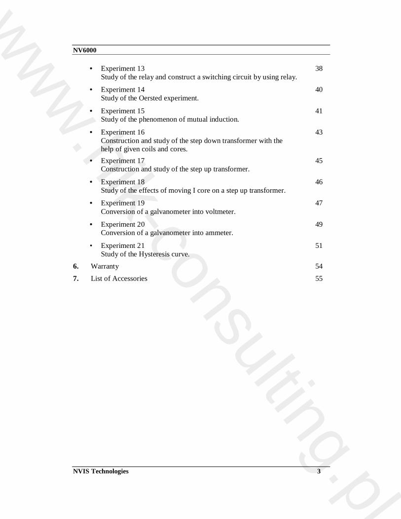
• Experiment 13 38 Study of the relay and construct a switching circuit by using relay.

• Experiment 14 40 Study of the Oersted experiment.

• Experiment 15 41 Study of the phenomenon of mutual induction.

• Experiment 16 43 Construction and study of the step down transformer with the help of given coils and cores.

• Experiment 17 45 Construction and study of the step up transformer.

• Experiment 18 46 Study of the effects of moving I core on a step up transformer.

• Experiment 19 47 Conversion of a galvanometer into voltmeter.

• Experiment 20 49 Conversion of a galvanometer into ammeter.

• Experiment 21 51 Study of the Hysteresis curve.

6. Warranty 54

7. List of Accessories 55


NV6000

NVIS Technologies 4

Introduction The NV6000 Electricity Lab is a versatile Training kit, for a laboratory. It is designed such that all the basic electrical circuits can be tested with the help of this trainer kit. The experiments given with training system develop mental starting from an introduction to the circuit, basic fundamentals and complete circuits like series and parallel circuits, electromagnetic induction, coil behaviors with AC and DC circuits diode and transistor characteristics etc. This simple training kit provides a strong foundation for future studies in electrical or electronics. This takes students from the basic of ohm’s law, through simple series and parallel circuit analysis and into same elementary aspects of electronics where they will build circuits using capacitors, transistor and diodes. Student can study how the resistance of a light bulb filament changes as it heats up.

With this system a set of coils and cores are provided. These high quality coils and laminated iron cores provides an effective introduction to electromagnetic theory. Each coil is labeled with number of turns. These can be used in study of 1. Electromagnetism : It shows how the magnetic field can be increased by

increasing the current, by adding an iron core or by using coil with more turns. 2. Induction : We can pass a magnet through a coil and detect the resulting

electromotive force with galvanometer. So it shows how the EMF depends on number of turns in the coil and on the relative velocity of the magnet and coil.

3. Transformers : We can mount coils on the U or E- shaped iron cores to demonstrate mutual induction. Then connect a load to investigate power transfer and basic transformers theory with an AC power supply. These are not ideal transformers. As is true for any transformer using separate coils, the flux linkage between coils is very less. The voltage transformation ratio are therefore proportionately below the ideal values based on the number of turns per coil within this limitation, effective quantitative investigations can be conducted using these coils and cores set.


NV6000

NVIS Technologies 5

Features

• Stand alone operation

• Durable, Easy to use kit

• Includes all the basic electrical fundamentals

• Solder less connection

• Complete set of coils and cores to understand the basics of electromagnetic induction and transformers

• Provided with a component box to perform all the experiments


NV6000

NVIS Technologies 6

Training Kit-Includes 1. Components box with

a. Resistors b. Capacitors

c. Transistors

d. Diode

e. Potentiometer 2. E, I, U cores

3. Set of coils 4. Magnetic compass

5. Bar magnets 6. Screw Driver

7. Multimeter 8. Connection patch cords


NV6000

NVIS Technologies 7

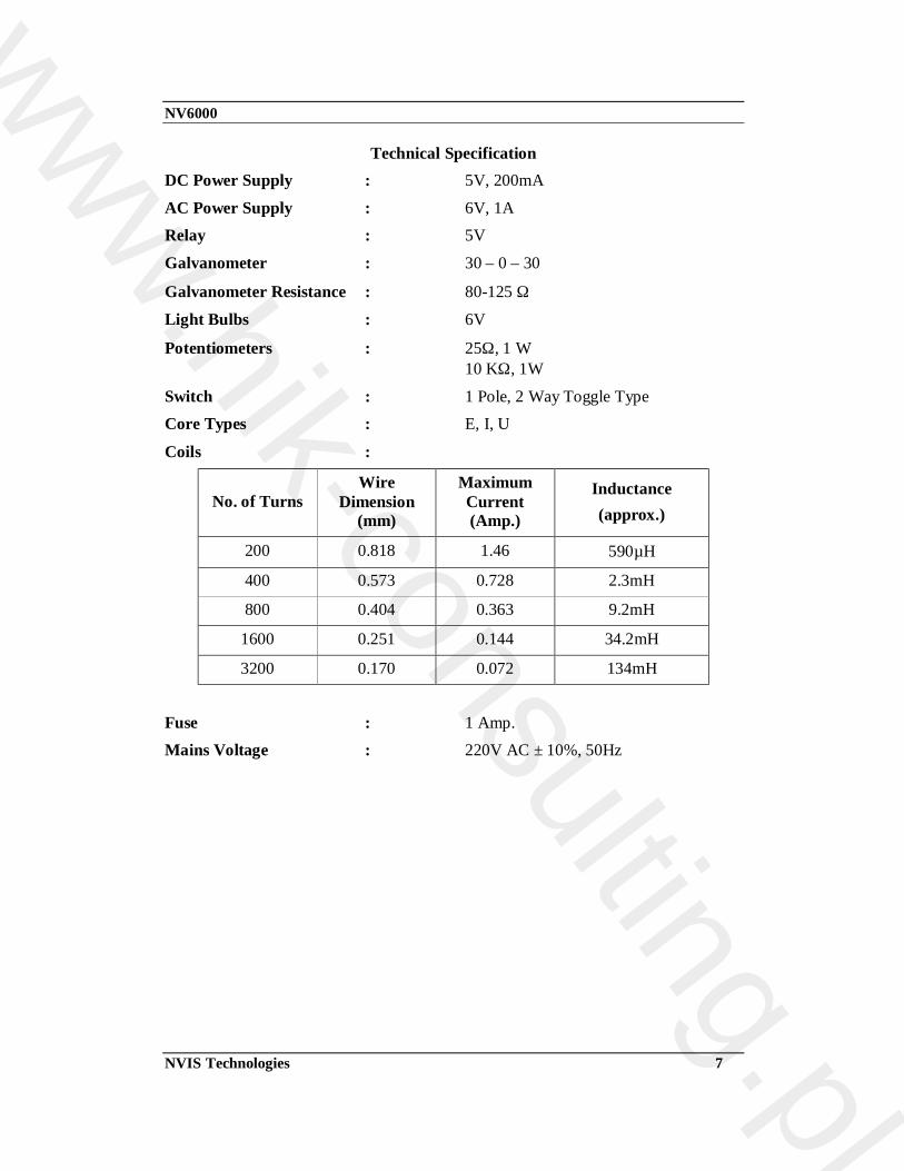
Technical Specification DC Power Supply : 5V, 200mA

AC Power Supply : 6V, 1A Relay : 5V Galvanometer : 30 – 0 – 30

Galvanometer Resistance : 80-125 Ω

Light Bulbs : 6V

Potentiometers : 25Ω, 1 W 10 KΩ, 1W

Switch : 1 Pole, 2 Way Toggle Type Core Types : E, I, U

Coils :

No. of Turns Wire

Dimension (mm)

Maximum Current (Amp.)

Inductance (approx.)

200 0.818 1.46 590µH

400 0.573 0.728 2.3mH

800 0.404 0.363 9.2mH

1600 0.251 0.144 34.2mH

3200 0.170 0.072 134mH

Fuse : 1 Amp. Mains Voltage : 220V AC ± 10%, 50Hz


NV6000

NVIS Technologies 8

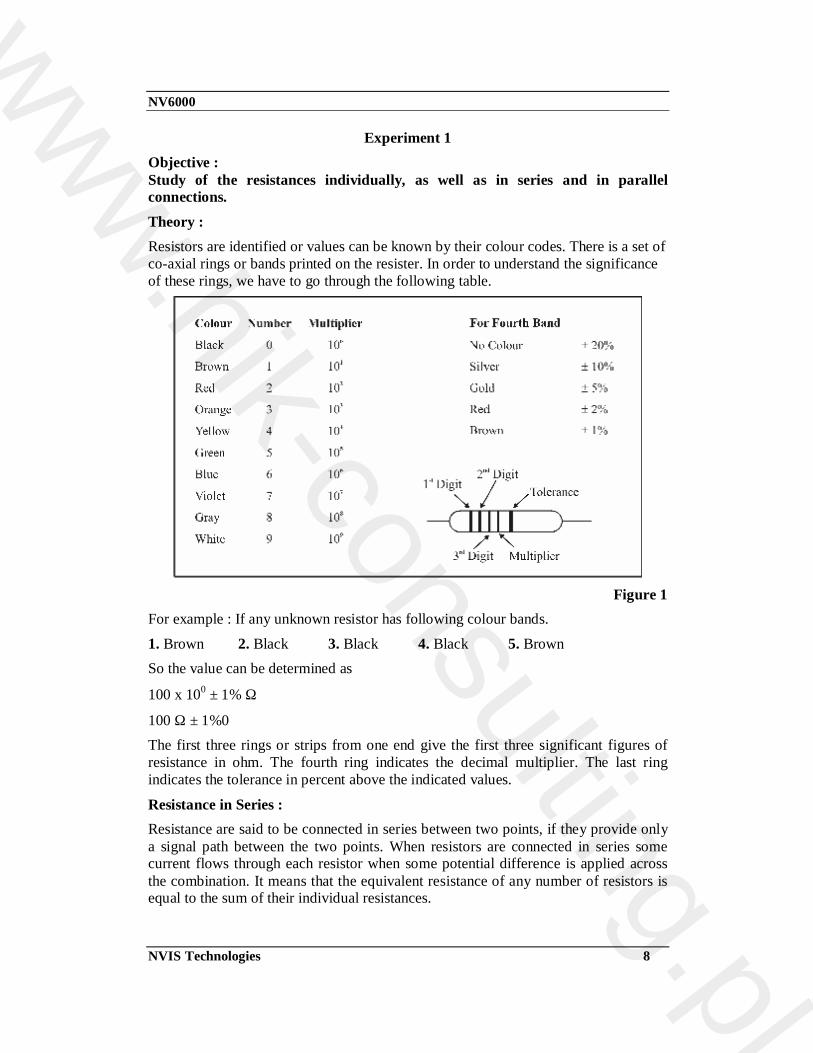
Experiment 1 Objective : Study of the resistances individually, as well as in series and in parallel connections. Theory : Resistors are identified or values can be known by their colour codes. There is a set of co-axial rings or bands printed on the resister. In order to understand the significance of these rings, we have to go through the following table.

Figure 1

For example : If any unknown resistor has following colour bands.

1. Brown 2. Black 3. Black 4. Black 5. Brown So the value can be determined as

100 x 100 ± 1% Ω

100 Ω ± 1%0 The first three rings or strips from one end give the first three significant figures of resistance in ohm. The fourth ring indicates the decimal multiplier. The last ring indicates the tolerance in percent above the indicated values.

Resistance in Series : Resistance are said to be connected in series between two points, if they provide only a signal path between the two points. When resistors are connected in series some current flows through each resistor when some potential difference is applied across the combination. It means that the equivalent resistance of any number of resistors is equal to the sum of their individual resistances.


NV6000

NVIS Technologies 9

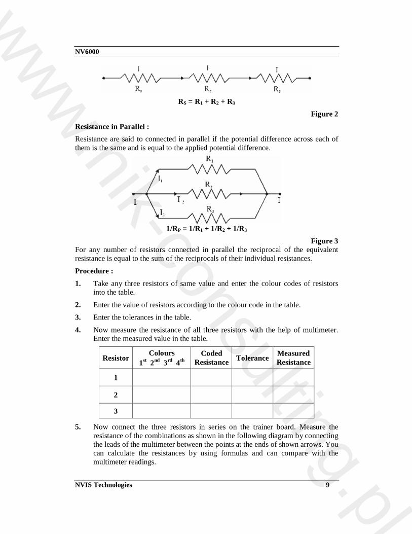
RS = R1 + R2 + R3

Figure 2 Resistance in Parallel : Resistance are said to connected in parallel if the potential difference across each of them is the same and is equal to the applied potential difference.

1/RP = 1/R1 + 1/R2 + 1/R3

Figure 3 For any number of resistors connected in parallel the reciprocal of the equivalent resistance is equal to the sum of the reciprocals of their individual resistances.

Procedure : 1. Take any three resistors of same value and enter the colour codes of resistors

into the table.

2. Enter the value of resistors according to the colour code in the table. 3. Enter the tolerances in the table.

4. Now measure the resistance of all three resistors with the help of multimeter. Enter the measured value in the table.

Resistor Colours 1st 2nd 3rd 4th

Coded Resistance Tolerance Measured

Resistance

1

2

3

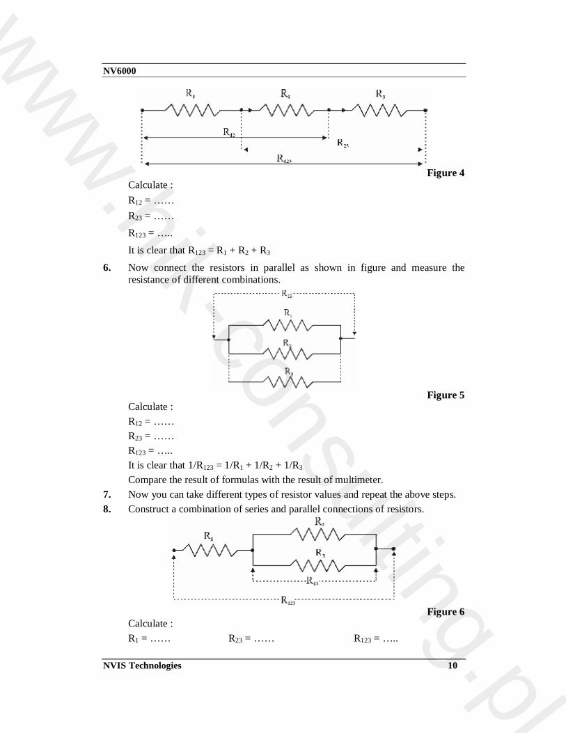
5. Now connect the three resistors in series on the trainer board. Measure the resistance of the combinations as shown in the following diagram by connecting the leads of the multimeter between the points at the ends of shown arrows. You can calculate the resistances by using formulas and can compare with the multimeter readings.


NV6000

NVIS Technologies 10

Figure 4

Calculate : R12 = …… R23 = …… R123 = …..

It is clear that R123 = R1 + R2 + R3

6. Now connect the resistors in parallel as shown in figure and measure the resistance of different combinations.

Figure 5

Calculate : R12 = …… R23 = …… R123 = ….. It is clear that 1/R123 = 1/R1 + 1/R2 + 1/R3 Compare the result of formulas with the result of multimeter.

7. Now you can take different types of resistor values and repeat the above steps. 8. Construct a combination of series and parallel connections of resistors.

Figure 6

Calculate : R1 = …… R23 = …… R123 = …..


NV6000


Experiment 2 Objective : Study of the ohm’s law mathematical relationship between three variables voltage (V), current (I) and resistance (R). Theory : We know that electric current is proportional to drift velocity which is turn in proportional to electric field strength. The electric field strength is proportional to potential difference. So the electric current is proportional to potential difference, which is ohm’s law. If V is the potential difference and I is the current, then V = IR where R = resistance

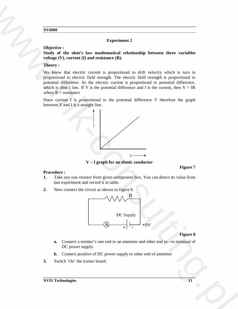
Since current I is proportional to the potential difference V therefore the graph between V and I is a straight line.

V – I graph for an ohmic conductor

Figure 7 Procedure : 1. Take any one resistor from given component box. You can detect its value from

last experiment and record it in table. 2. Now connect the circuit as shown in figure 8.

Figure 8

a. Connect a resister’s one end to an ammeter and other end to –ve terminal of DC power supply.

b. Connect positive of DC power supply to other end of ammeter. 3. Switch ‘On’ the trainer board.


NV6000


4. Set the multimeter to the appropriate range and measure the current flowing through the resistance. Record this value of current in the table.

Note : when current is to be measure we have to connect ammeter (multimeter) in series.

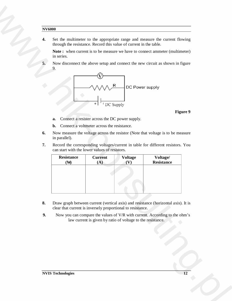
5. Now disconnect the above setup and connect the new circuit as shown in figure 9.

Figure 9

a. Connect a resister across the DC power supply. b. Connect a voltmeter across the resistance.

6. Now measure the voltage across the resistor (Note that voltage is to be measure in parallel).

7. Record the corresponding voltages/current in table for different resistors. You can start with the lower values of resistors.

Resistance (Ω)

Current (A)

Voltage (V)

Voltage/ Resistance

8. Draw graph between current (vertical axis) and resistance (horizontal axis). It is

clear that current is inversely proportional to resistance. 9. Now you can compare the values of V/R with current. According to the ohm’s

law current is given by ratio of voltage to the resistance.


NV6000


Experiment 3 Objective : Study of the voltage and current flowing into the circuit. Theory : In any series circuit the voltage is distributed according to the size of the resistor. It means that for high value of resistance a high voltage drop will be there and for a low value resistance low voltage drop will be there. In any parallel circuit the voltage is the same across all the elements of parallel combination. It means parallel resistances represent a single resistance and that’s why the same voltage drop is there. In combination of series and parallel circuits the parallel resistors were actually one resistor, which is then in series with the first then the rules are same as above.

In series circuit the current is same for all values of resistance. But in parallel circuit current is not same in all the branches it will be different for different resistances. In any resistance circuit series or parallel or both the voltage, current and resistance are related by ohm’s law. i.e. V = IR This can be observed in results.

Procedure : 1. Connect the three resistors of same value in the series circuit as shown in figure

10, connect the DC power supply across it.

Figure 10

2. Measure the voltage drop across the resistance and series combinations with the help of multimeter.

R1 = V1 = R2 = V2 =

R3 = V3 =

R12 = V12 =

R23 = V23 = R123 = V123 =

Repeat the steps with different values of resistors.


NV6000


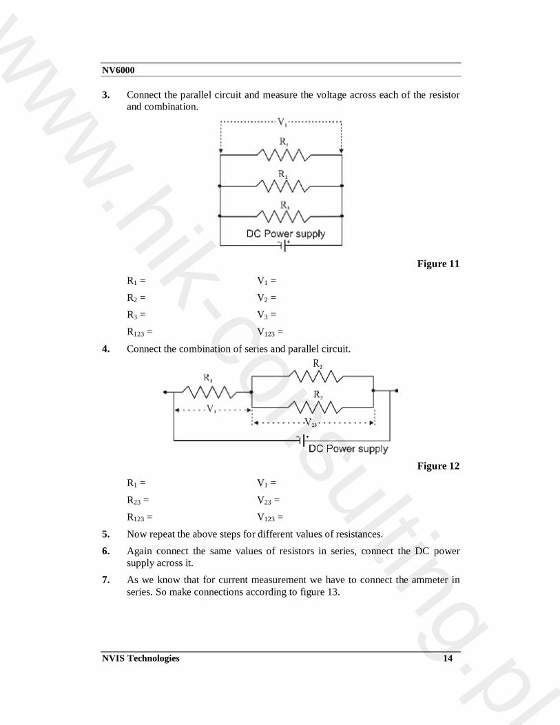
3. Connect the parallel circuit and measure the voltage across each of the resistor and combination.

Figure 11

R1 = V1 =

R2 = V2 = R3 = V3 =

R123 = V123 =

4. Connect the combination of series and parallel circuit.

Figure 12

R1 = V1 =

R23 = V23 = R123 = V123 =

5. Now repeat the above steps for different values of resistances. 6. Again connect the same values of resistors in series, connect the DC power

supply across it. 7. As we know that for current measurement we have to connect the ammeter in

series. So make connections according to figure 13. www.hik-consulting.pl

NV6000


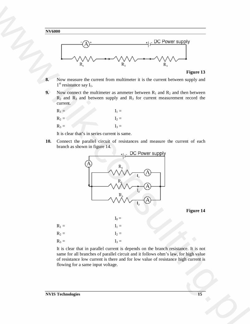
Figure 13

8. Now measure the current from multimeter it is the current between supply and 1st resistance say I1.

9. Now connect the multimeter as ammeter between R1 and R2 and then between R2 and R3 and between supply and R3 for current measurement record the current.

R1 = I1 = R2 = I2 =

R3 = I3 = It is clear that’s in series current is same.

10. Connect the parallel circuit of resistances and measure the current of each branch as shown in figure 14.

Figure 14

I0 =

R1 = I1 = R2 = I2 =

R3 = I3 = It is clear that in parallel current is depends on the branch resistance. It is not same for all branches of parallel circuit and it follows ohm’s law, for high value of resistance low current is there and for low value of resistance high current is flowing for a same input voltage.


NV6000


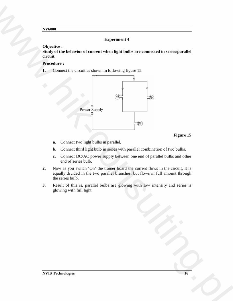
Experiment 4 Objective : Study of the behavior of current when light bulbs are connected in series/parallel circuit. Procedure : 1. Connect the circuit as shown in following figure 15.

Figure 15

a. Connect two light bulbs in parallel. b. Connect third light bulb in series with parallel combination of two bulbs.

c. Connect DC/AC power supply between one end of parallel bulbs and other end of series bulb.

2. Now as you switch ‘On’ the trainer board the current flows in the circuit. It is equally divided in the two parallel branches, but flows in full amount through the series bulb.

3. Result of this is, parallel bulbs are glowing with low intensity and series is glowing with full light.


NV6000


Experiment 5 Objective : Study of the Kirchhoff’s Law for electrical circuits. Theory : Kirchhoff’s laws are simply the expression of conservation of electric charge and of energy. There are two famous rules developed by Gustav Robert Kirchhoff in the year 1842. After him these rules are known as Kirchhoff’s rules.

Kirchhoff First Law or Kirchhoff’s current law or junction rule : In any electrical network the algebraic sum of currents meeting at a junction is always zero.

Σ I = 0 The currents directed towards the junction are taken as positive while those directed towards away from the junction are taken as negative.

I1 + I2 – I3 – I4 – I5 = 0

I1 + I2 = I3 – I4 – I5

Figure 16 From above expression we can say that the sum of current flowing towards the junction is equal to the sum of currents leaving the junction.

Kirchhoff’s Second Law or Kirchhoff’s voltage law or loop rule : The algebraic sum of all the potential drops around a closed loop is equal to the sum of the voltage sources of that loop. This voltage law gives the relationship between the ‘voltage drops’ around any closed loop in a circuit and the voltage sources in that loop. The total of these two quantities is always equal. Equation can be given by

E source = E1 + E2 + E3 = I1R1 + I2 R2 + I3 R3

Σ E = Σ IR

i.e. Kirchhoff’s voltage law can be applied only to closed loop. A closed loop must meet two conditions.

1. It must have one or more voltage sources.


NV6000


2. It must have a complete path for current flow from any point, around the loop and back to that point.

Procedure : 1. Connect the following circuit.

Figure 17

a. Connect R1 (330Ω) to +ve end of supply and its other end to one ends of R2 (220Ω) and R5 (100Ω).

b. Connect other end of R2 to one ends of R3 (200Ω) and R6 (100Ω)

c. Now connect other end of R3 to one ends of R4 (100Ω) and R7 (100Ω)

d. Connect other end of R4 to one end of R8 (100Ω)

e. Connect other end of R8 to one end of R9 (100Ω) f. Connect other end of R9 to other ends of R7, R6, R5 and to one end of R10

(100Ω) g. Connect other end of R10 to –ve end of power supply.

2. Now for testing the KCL at node ‘B’ we have to measure the following. 3. First remove supply connection to R1, now measure incoming current Iin

between +ve end of source and first end of resistor R1 i.e., connect the multimeter as ammeter between these two points.

Note : whenever we have to measure the current in the branch, we have to connect the ammeter in series and after measuring the current disconnect the ammeter and make the connection as previous.

4. Measure outgoing current I1 between second end of R5 (when this terminal is not connected to trainer) and common end of R10 and R9.

5. Measure outgoing current I2 between second end of R2 (when this terminal is not connected to trainer) and junction of R3 and R6.

6. Check whether the incoming current Iin is equal to the sum of outgoing current (I1 & I2).


NV6000


7. Repeat the procedure for junction point C, D, G, H, I.

To test the KVL in the loop ABIJ measure the following :

1. Measure current Iin following through resistor of 330Ω with the help of ammeter as step (3).

2. Measure current I1 as step 4.

3. Measure current Iout between point J and one end of resistor R10. 4. Calculate the different IR drops in the ABIJ loop (sign of IR drops should be

given after considering direction of current.)

5. Measure the sum of IR drop with their sign. 6. Equate the sum of all IR drops (with their sign) and sum of the source voltage of

that particular loop it should be equal. 7. In case of no voltage source in loop take the sum of all voltage source equal to

zero. 8. Repeat above procedure for loop BCHI, CDGH, DEFG.


NV6000


Experiment 6 Objective : Study of the R-C circuit and find out the behavior of capacitor in a R-C network and study the phase shift due to capacitor. Theory : The Capacitor : A capacitor is a device that can store electrical charge. The simplest kind is a "parallel plate" capacitor that consists of two metal plates that are separated by an insulating material such as dry air, plastic or ceramic. Such a device is shown schematically below figure 18.

A simple capacitor circuit

Figure 18 It is straightforward to see how it could store electrical energy. If we connect the two plates to each other with a battery in the circuit, as shown in the figure above, the battery will drive charge around the circuit as an electric current. But when the charges reach the plates they can't go any further because of the insulating gap; they collect on the plates, one plate becoming positively charged and the other negatively charged. The voltage across the plates due to the electric charges is opposite in sign to the voltage of the battery. As the charge on the plates builds up, this back-voltage increases, opposing the action of the battery. As a consequence, the current flowing in the circuit decays, falling to zero when the back-voltage is exactly equal and opposite to the battery voltage. If we quickly remove the wires without touching the plates, the charge remains on the plates. Because the two plates have different charge, there is a net electric field between the two plates. Hence, there is a voltage difference between the plates. If, sometime later, we connect the plates again, this time with a light bulb in place of the battery, the plates will discharge: the electrons on the negatively charged plate will move around the circuit to the positive plate until all the charges are equalized. During this short discharge period a current is flowing and the bulb will light. The capacitor stored electrical energy from its original charge up by the battery until it could discharge through the light bulb. The speed with which the discharge (and conversely the charging process) can take place is limited by the resistance of the circuit connecting the plates and by the capacitance of the capacitor (a measure of its ability to hold charge). An RC circuit is simply a circuit with a voltage source (battery) connected in series with a resistor and a capacitor.


NV6000


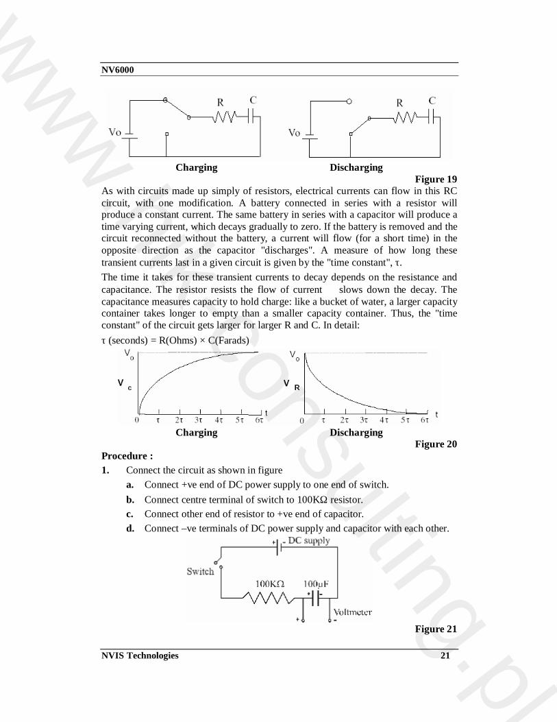
Charging Discharging

Figure 19 As with circuits made up simply of resistors, electrical currents can flow in this RC circuit, with one modification. A battery connected in series with a resistor will produce a constant current. The same battery in series with a capacitor will produce a time varying current, which decays gradually to zero. If the battery is removed and the circuit reconnected without the battery, a current will flow (for a short time) in the opposite direction as the capacitor "discharges". A measure of how long these transient currents last in a given circuit is given by the "time constant", τ. The time it takes for these transient currents to decay depends on the resistance and capacitance. The resistor resists the flow of current ⇒ slows down the decay. The capacitance measures capacity to hold charge: like a bucket of water, a larger capacity container takes longer to empty than a smaller capacity container. Thus, the "time constant" of the circuit gets larger for larger R and C. In detail: τ (seconds) = R(Ohms) × C(Farads)

Charging Discharging

Figure 20 Procedure : 1. Connect the circuit as shown in figure

a. Connect +ve end of DC power supply to one end of switch. b. Connect centre terminal of switch to 100KΩ resistor. c. Connect other end of resistor to +ve end of capacitor. d. Connect –ve terminals of DC power supply and capacitor with each other.

Figure 21


NV6000


2. Switch ‘On’ the trainer board. 3. Put the toggle switch in ‘Off’ condition, if there is some remaining voltage on

the capacitor, use a piece of wire to short the two leads together draining any remaining charge, i.e. discharge the capacitor.

4. Now if you put the toggle switch in ON condition you can observe voltmeter that the capacitor is charging very fast but after few second the rate of charging is slow.

5. Now put the toggle switch in ‘Off’ condition and connect a wire from 1st end of resistor to 2nd end of capacitor. Here we can observe the charge is flowing back. In start it discharges very fast but after few seconds discharging is slow.

6. You can record the time of charging tc and time of discharging td for a given value of resistor and capacitor. Now you can change the value of resistors and capacitors and record the values of tc and td in the table.

No. Resistance Capacitance tc td 1 2 3 4

Phase Shift : 1. Replace the electrolytic capacitor of previous circuit with metallic polyester

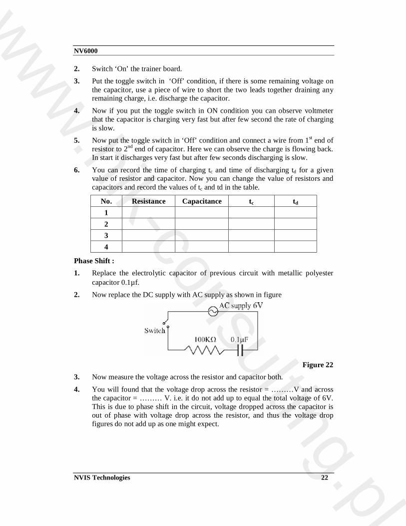
capacitor 0.1µf. 2. Now replace the DC supply with AC supply as shown in figure

Figure 22

3. Now measure the voltage across the resistor and capacitor both.

4. You will found that the voltage drop across the resistor = ………V and across the capacitor = ……… V. i.e. it do not add up to equal the total voltage of 6V. This is due to phase shift in the circuit, voltage dropped across the capacitor is out of phase with voltage drop across the resistor, and thus the voltage drop figures do not add up as one might expect.


NV6000


Experiment 7

Objective : Study of the L-C circuit and its oscillations. Theory : Let us assume that initially the capacitor C of the LC circuit carries a charge Q and the current I in the inductor is zero.

At this instant, the energy stored in the electric field of the capacitor is

UE =

C

Q2

2

. The energy stored in the inductor is zero.

The capacitor now begins to discharge through the inductor. The current begins to flow counter-clockwise. As the charge on the capacitor decreases, UE decreases. But

the energy UB =

2

21 LI in the magnetic field of the inductor increases. The energy

is transferred from the capacitor to the inductor.

The energy stored in the capacitor is transferred entirely to the magnetic field of the inductor. At this stage, there is maximum value of current in the inductor. This current continues to transport positive charge from the top plate of the capacitor to the bottom plate of the capacitor. Energy now flows from the inductor back to the capacitor as the electric field builds up again. The capacitor will begin to discharge again. The current will now flow clockwise. Proceeding as before, we find that the circuit eventually returns to the situation depicted. The process continues at a definite frequency. The energy is continuously shuttled back and forth between the electric field in the capacitor and the magnetic field in the inductor.

In an actual LC circuit, some resistance is always present. This resistance will drain energy from the electric and magnetic fields and dissipate it as thermal energy will not continue indefinite

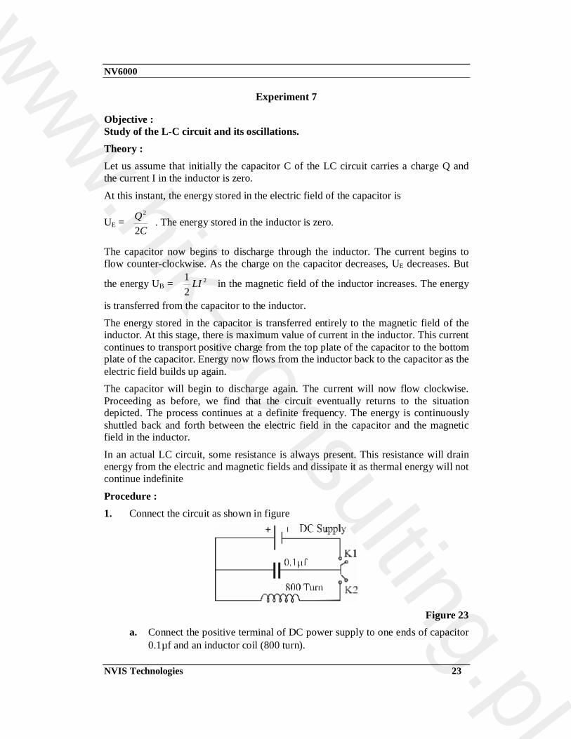
Procedure : 1. Connect the circuit as shown in figure

Figure 23

a. Connect the positive terminal of DC power supply to one ends of capacitor 0.1µf and an inductor coil (800 turn).


NV6000


b. Connect other end of capacitor to negative of DC power supply through a switch (1st and common end of switch)

c. Connect other end of coil to third end of switch (which acts as a second switch).

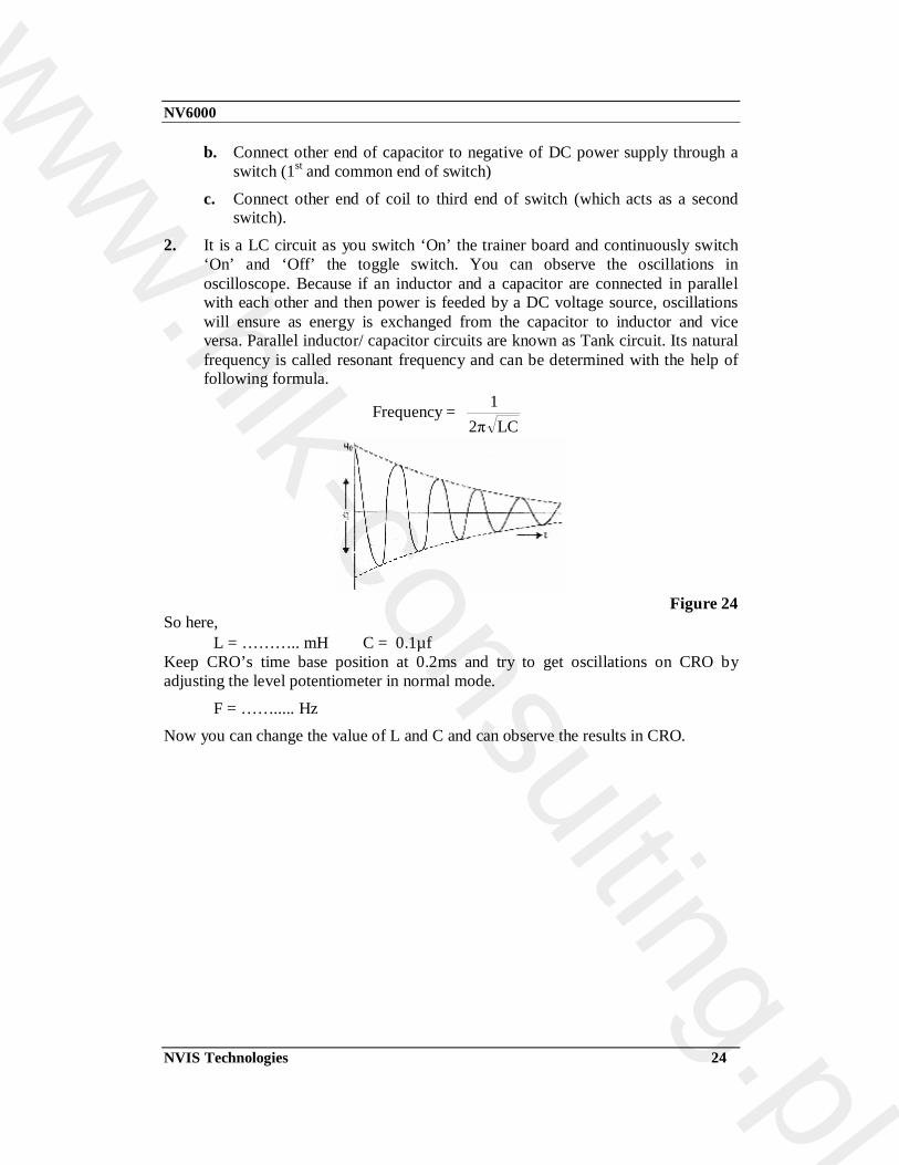
2. It is a LC circuit as you switch ‘On’ the trainer board and continuously switch ‘On’ and ‘Off’ the toggle switch. You can observe the oscillations in oscilloscope. Because if an inductor and a capacitor are connected in parallel with each other and then power is feeded by a DC voltage source, oscillations will ensure as energy is exchanged from the capacitor to inductor and vice versa. Parallel inductor/ capacitor circuits are known as Tank circuit. Its natural frequency is called resonant frequency and can be determined with the help of following formula.

=

LC2π1Frequency

Figure 24

So here, L = ……….. mH C = 0.1µf

Keep CRO’s time base position at 0.2ms and try to get oscillations on CRO by adjusting the level potentiometer in normal mode.

F = ……..... Hz Now you can change the value of L and C and can observe the results in CRO.


NV6000


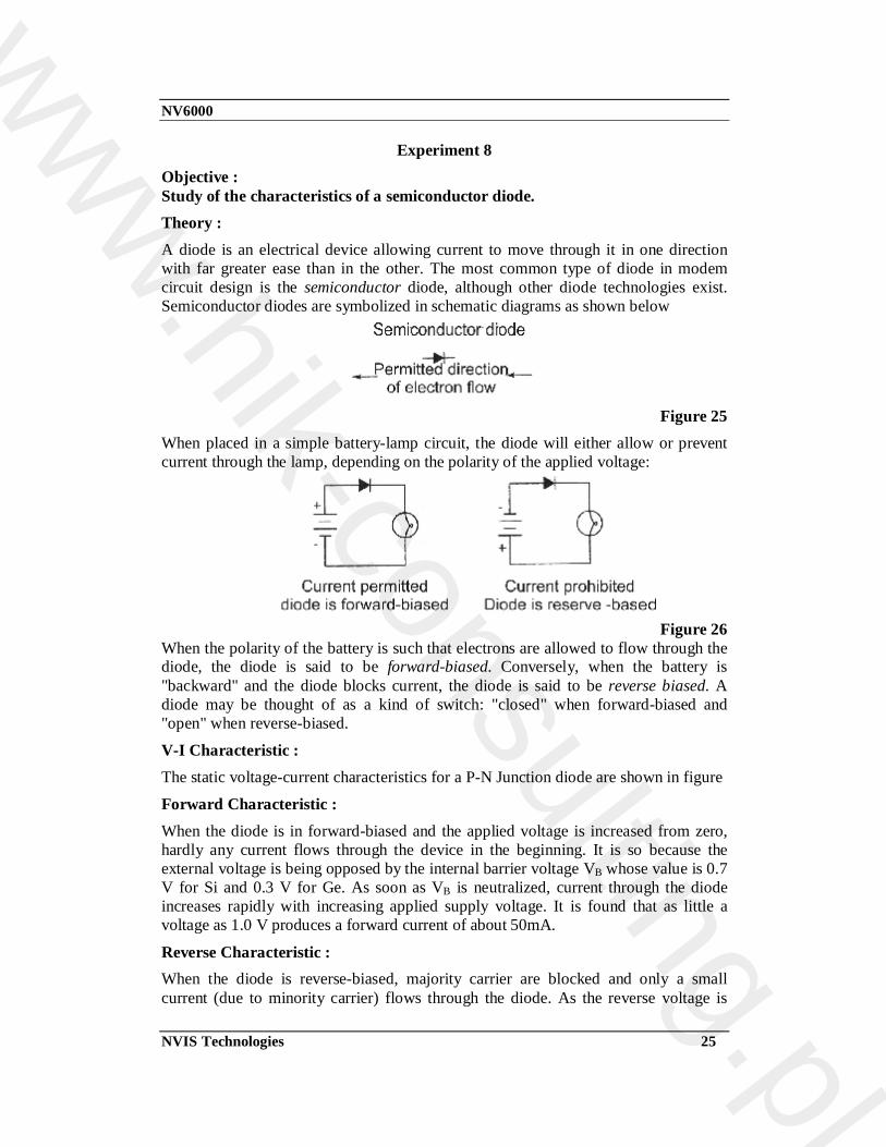
Experiment 8 Objective : Study of the characteristics of a semiconductor diode. Theory : A diode is an electrical device allowing current to move through it in one direction with far greater ease than in the other. The most common type of diode in modem circuit design is the semiconductor diode, although other diode technologies exist. Semiconductor diodes are symbolized in schematic diagrams as shown below

Figure 25

When placed in a simple battery-lamp circuit, the diode will either allow or prevent current through the lamp, depending on the polarity of the applied voltage:

Figure 26

When the polarity of the battery is such that electrons are allowed to flow through the diode, the diode is said to be forward-biased. Conversely, when the battery is "backward" and the diode blocks current, the diode is said to be reverse biased. A diode may be thought of as a kind of switch: "closed" when forward-biased and "open" when reverse-biased.

V-I Characteristic : The static voltage-current characteristics for a P-N Junction diode are shown in figure

Forward Characteristic : When the diode is in forward-biased and the applied voltage is increased from zero, hardly any current flows through the device in the beginning. It is so because the external voltage is being opposed by the internal barrier voltage VB whose value is 0.7 V for Si and 0.3 V for Ge. As soon as VB is neutralized, current through the diode increases rapidly with increasing applied supply voltage. It is found that as little a voltage as 1.0 V produces a forward current of about 50mA.

Reverse Characteristic : When the diode is reverse-biased, majority carrier are blocked and only a small current (due to minority carrier) flows through the diode. As the reverse voltage is


NV6000


increased from zero, the reverse current very quickly reaches its maximum or saturation value Io which is also known as leakage current. It is of the order of nanoamperes (nA) and microamperes (µA) for Ge.

Procedure : 1. Connect the circuit as shown in figure 27.

Figure 27

a. Connect +ve terminal of DC power supply to one end of potentiometer. b. Connect middle terminal of potentiometer to one end of resistor 1K.

c. Connect other terminal of resister to +ve end (Black end) of diode IN4007. d. Connect –ve terminal of DC power supply to other end of potentiometer.

2. Now rotate the potentiometer fully clockwise position. 3. Connect one multimeter (at voltmeter range) point A and B it means across the

diode. 4. Now connect the multimeter (as ammeter) between –ve terminal of diode and

ground, it means we have to connect it in series with diode.

Figure 28

5. Switch ‘On’ the power supply. 6. Vary the potentiometer so as to increase the value of diode voltage VD in the

steps of 100mV. 7. Now record the diode current ID (mA) with corresponding diode voltage VD in

table.

S. No. Diode Voltage VD

Diode Current ID (mA)


NV6000


8. Plot a curve between diode voltage VD and current ID as shown in figure (1st quadrant) using suitable scale with the help of observation table. This curve is required forward characteristics of Si diode.

Figure 29

For Reverse Characteristics : For this experiment only the polarity of diode will be reversed. 1. Measure the diode voltage VD in steps of 1 Volt, and corresponding diode

current same as the previous given procedure. 2. Plot a curve between diode voltage VD and diode current ID as shown in figure

29 (3rd quadrant). This curve is required characteristics of Si diode.


NV6000


Experiment 9 Objective : Study of the characteristics of a transistor. Theory : Transistor characteristics are the curves, which represent relationship between different dc currents and voltages of a transistor. These are helpful in studying the operation of a transistor when connected in a circuit. The three important characteristics of a transistor are: 1. Input characteristic.

2. Output characteristic. 3. Constant current transfer characteristic.

Input Characteristic : In common emitter configuration, it is the curve plotted between the input current (IB) verses input voltage (VBE) for various constant values of output voltage (VCE). The approximated plot for input characteristic is shown in figure 30. This characteristic reveal that for fixed value of output voltage VCE, as the base to emitter voltage increases, the emitter current increases in a manner that closely resembles the diode characteristics.

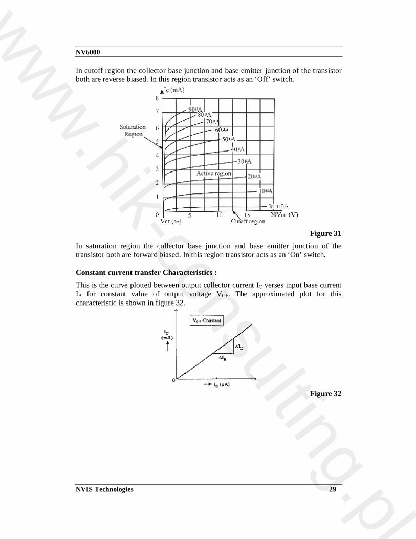
Figure 30 Output Characteristic : This is the curve plotted between the output current IC verses output voltage VCE for various constant values of input current IB.

The output characteristic has three basic region of interest as indicated in figure 31. The active region, cutoff region and saturation region.

In active region the collector base junction is reverse biased while the base emitter junction if forward biased. This region is normally employed for linear (undistorted) amplifier.


NV6000


In cutoff region the collector base junction and base emitter junction of the transistor both are reverse biased. In this region transistor acts as an ‘Off’ switch.

Figure 31

In saturation region the collector base junction and base emitter junction of the transistor both are forward biased. In this region transistor acts as an ‘On’ switch. Constant current transfer Characteristics : This is the curve plotted between output collector current IC verses input base current IB for constant value of output voltage VCE. The approximated plot for this characteristic is shown in figure 32.

Figure 32


NV6000


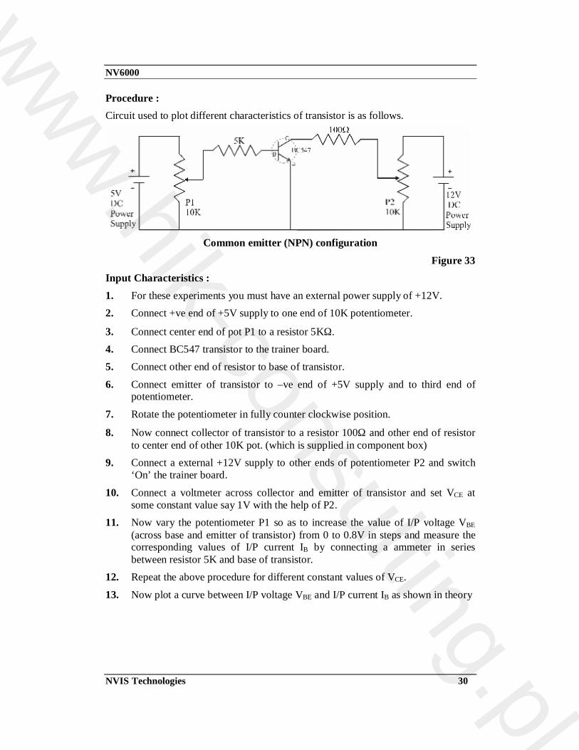
Procedure : Circuit used to plot different characteristics of transistor is as follows.

Common emitter (NPN) configuration

Figure 33 Input Characteristics : 1. For these experiments you must have an external power supply of +12V. 2. Connect +ve end of +5V supply to one end of 10K potentiometer.

3. Connect center end of pot P1 to a resistor 5KΩ. 4. Connect BC547 transistor to the trainer board. 5. Connect other end of resistor to base of transistor.

6. Connect emitter of transistor to –ve end of +5V supply and to third end of potentiometer.

7. Rotate the potentiometer in fully counter clockwise position.

8. Now connect collector of transistor to a resistor 100Ω and other end of resistor to center end of other 10K pot. (which is supplied in component box)

9. Connect a external +12V supply to other ends of potentiometer P2 and switch ‘On’ the trainer board.

10. Connect a voltmeter across collector and emitter of transistor and set VCE at some constant value say 1V with the help of P2.

11. Now vary the potentiometer P1 so as to increase the value of I/P voltage VBE (across base and emitter of transistor) from 0 to 0.8V in steps and measure the corresponding values of I/P current IB by connecting a ammeter in series between resistor 5K and base of transistor.

12. Repeat the above procedure for different constant values of VCE.

13. Now plot a curve between I/P voltage VBE and I/P current IB as shown in theory www.hik-consulting.pl

NV6000


Observation Table :

Input current IB (uA) at constant value of output voltage S. No.

Input voltage VBE

VCE = 1V VCE = 3V VCE =5V

1. 0.0V

2. 0.1V

3. 0.2V

4. 0.3V

5. 0.4V

6. 0.5V

7. 0.6V

8. 0.7V

9. 0.8V

Output Characteristics : 1. Switch ‘Off’ the supply. 2. Rotate both the potentiometer P1 and P2 in fully counter clockwise position.

3. Switch ‘On’ the power supply. 4. Vary the potentiometer and set a value of I/P current IB at some constant value

say (0µA, 10µA, ….. 100µA) by connecting a meter between resistor 5K and base of transistor.

5. Vary the potentiometer P2 so as to increase the value of O/P voltage VCE from 0 to maximum value in steps and measure the output current IC by connecting ammeter between collector of transistor and 100Ω resistor.

6. Repeat the procedure for different values of I/P current IB. 7. Plot a curve between O/P voltage VCE and O/p current IC as shown in theory.


NV6000


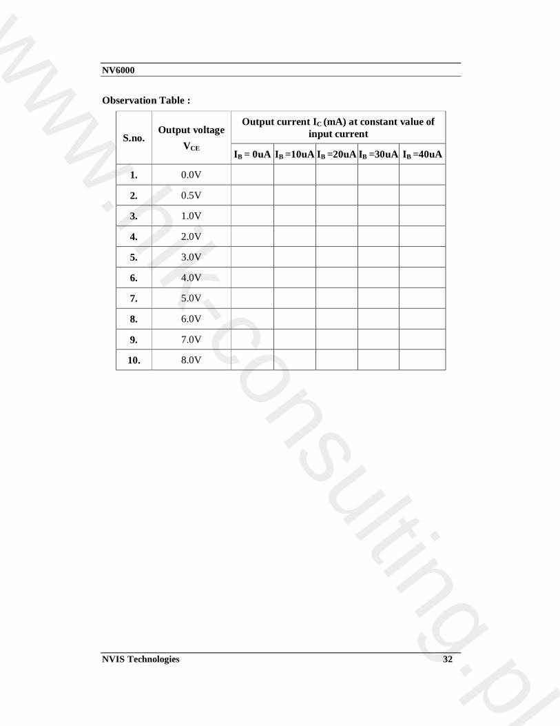
Observation Table :

Output current IC (mA) at constant value of input current S.no.

Output voltage VCE

IB = 0uA IB =10uA IB =20uA IB =30uA IB =40uA

1. 0.0V

2. 0.5V

3. 1.0V

4. 2.0V

5. 3.0V

6. 4.0V

7. 5.0V

8. 6.0V

9. 7.0V

10. 8.0V


NV6000


Experiment 10 Objective : Understanding the Faraday’s Law of electromagnetic induction. Whenever there is a change in the magnetic flux linked with a circuit an emf and consequently a current is induced in the circuit. However, it lasts only so long as the magnetic flux is changing.

Procedure : 1. Take any coil from the given coil set and let the two ends of the coil be

connected to the two terminal of galvanometer.

Figure 34

2. Now take a bar magnet and keep its north pole stationary near one end of coil as shown in figure 34. The galvanometer shall not show any deflection. When magnet is stationary.

3. When the magnet is moved toward the coil, the galvanometer shows deflection as shown in figure 35.

Figure 35

4. When the magnet is moved away from the coil, the galvanometer again shows deflection but in opposite direction.

5. Similar results are obtained when the magnet is kept stationary and the coil is moved.


NV6000


6. When the magnet is moved slowly the deflection in meter is small, but when the magnet is moved fast the deflection is large.

7. It is clear from above experiment that when magnetic flux. Changes through a coil, a current are induced in the coil.

8. Observe the results for different coils.


NV6000


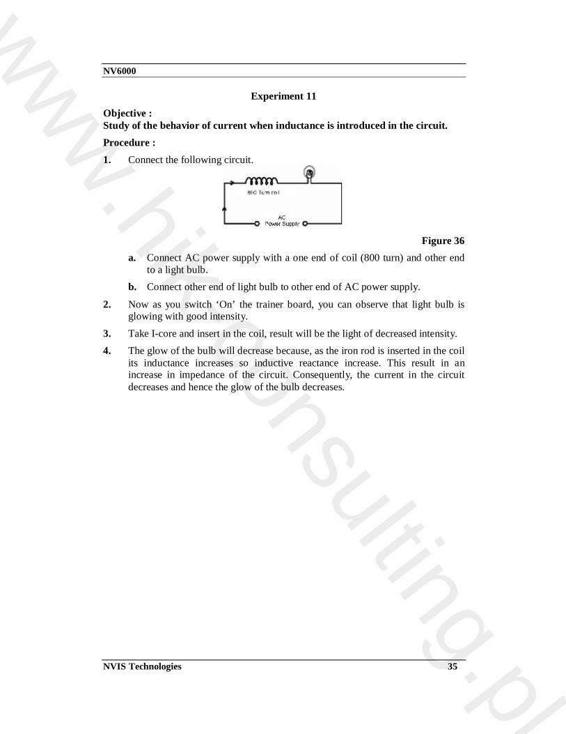
Experiment 11 Objective : Study of the behavior of current when inductance is introduced in the circuit. Procedure : 1. Connect the following circuit.

Figure 36

a. Connect AC power supply with a one end of coil (800 turn) and other end to a light bulb.

b. Connect other end of light bulb to other end of AC power supply.

2. Now as you switch ‘On’ the trainer board, you can observe that light bulb is glowing with good intensity.

3. Take I-core and insert in the coil, result will be the light of decreased intensity. 4. The glow of the bulb will decrease because, as the iron rod is inserted in the coil

its inductance increases so inductive reactance increase. This result in an increase in impedance of the circuit. Consequently, the current in the circuit decreases and hence the glow of the bulb decreases.


NV6000


Experiment 12 Objective : Study of the Lenz’s Law and effect of eddy current. The induced current produced in the conductor always flows in such a direction that the magnetic field it produces will oppose the change that is producing it.

Lenz’s law states that in a given circuit with an induced emf caused by a change in a magnetic flux, the induced emf causes a current to flow in the direction that oppose the change in flux. That is if a decreasing magnetic flux induces an emf, the resulting current will oppose a further decrease in magnetic flux. Likewise for an emf induced by an increasing magnetic flux, the resulting current flows in a direction that opposes a further increase in magnetic flux. ‘when the north pole of the magnet is moved towards the coil, the direction of the induced current in the coil will be such that the upper face of the coil acquired north polarity. So the coil repels the magnet. In other words, the coil oppose the motion of the magnet towards itself which is really the cause of the induced current in the coil. Similarly, if the south pole of a magnet is moved towards the coil, the upper face of the coil will acquire south polarity there by opposing the motion of the magnet.

Eddy Current : Eddy current may be defined as current induced in a thick conductor when the conductor is placed in a changing magnetic field. Consider a metal block placed in a continuously varying magnetic field. The magnetic field can be changed either by having a permanent magnetic field and moving the block in and out of it or by keeping the block fixed and changing the magnetic field with the help of an alternating current. Due to the continuous change of magnetic flux linked with the metal block, induced current will be setup in the body of the metal block itself.

These current assume a circular path and their direction is given by Lenz’s law. These current look like eddies in a fluid and hence called eddy current. Since the resistance of this conductor is quite low therefore the eddy current are generally quite large in magnitude and produces heating effect. In following experiment, we will see its effect.

Procedure : 1. Take a 400 turn coil.

2. Fix a U-core into the bracket given on the trainer board. 3. Insert the coil in any end of U core.

4. Connect one end of coil to positive terminal of DC power supply and other to the one terminal of switch.


NV6000


Figure 37

5. Connect –ve terminal of power supply to other end of switch.

6. Let the toggle switch in ‘Off’ (upward direction if first two terminals are used) condition.

7. Take a soft iron square piece from the accessories and put it on the upper base of U-core where coil is connected.

8. Switch ‘On’ the trainer board. As you switch ‘On’ the toggle switch the metallic piece is thrown up. Because when the current begins to grow through the coil, the magnetic flux through the core and hence metallic piece begins to increase. This sets up eddy currents in the metallic piece. If the upper face of the core acquires N polarity in it then the lower face of the metallic piece also acquires N polarity according to the Lenz’s law. Due to force of repulsion between same poles, the metallic piece is thrown up.


NV6000


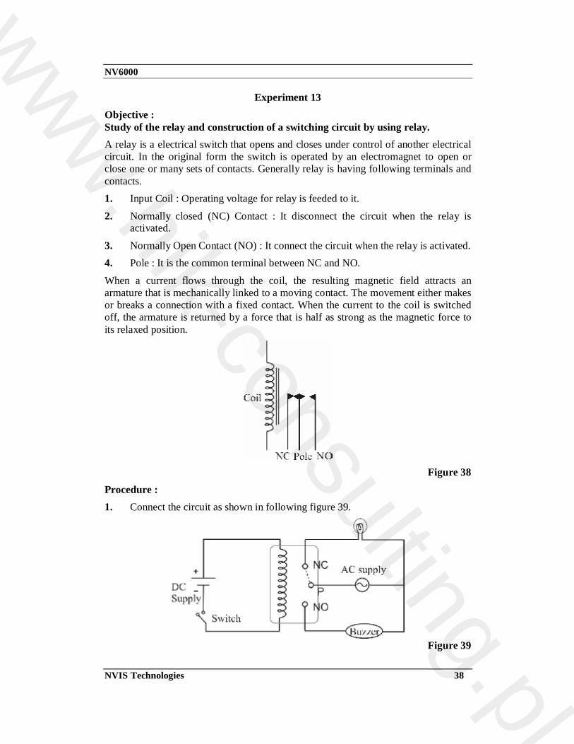
Experiment 13 Objective : Study of the relay and construction of a switching circuit by using relay. A relay is a electrical switch that opens and closes under control of another electrical circuit. In the original form the switch is operated by an electromagnet to open or close one or many sets of contacts. Generally relay is having following terminals and contacts. 1. Input Coil : Operating voltage for relay is feeded to it.

2. Normally closed (NC) Contact : It disconnect the circuit when the relay is activated.

3. Normally Open Contact (NO) : It connect the circuit when the relay is activated. 4. Pole : It is the common terminal between NC and NO.

When a current flows through the coil, the resulting magnetic field attracts an armature that is mechanically linked to a moving contact. The movement either makes or breaks a connection with a fixed contact. When the current to the coil is switched off, the armature is returned by a force that is half as strong as the magnetic force to its relaxed position.

Figure 38

Procedure : 1. Connect the circuit as shown in following figure 39.

Figure 39


NV6000


a. Connect positive terminal of DC power supply to one end of coil and negative terminal to other end of coil through a toggle switch.

b. Connect pole to any one terminal of AC power supply. c. Connect NO terminal to one end of Buzzer and NC terminal of relay to one

end of a light bulb.

d. Connect other end of AC power supply with other ends of Buzzer and light bulb.

2. Keep the toggle switch in off condition.

3. Now switch ‘On’ the power supply. In this condition relay coil is not getting supply voltage so the pole and NC terminals are shorted with each other and since we have connected a light bulb with this terminals in series with a AC power supply so it gets lightened.

4. Now as you turn ‘On’ the toggle switch, coil of relay will get supply voltage =5V and hence the NC point of relay is separated from pole and NO point of relay attracted towards pole and make contact with pole. Since we have connected a buzzer with these terminals in series with an AC power supply so buzzer gives the sound of frequency 50 Hz.


NV6000


Experiment 14 Objective : Study of the Oersted experiment. The connection between electricity and magnetism was rediscovered by a Danish physicist Hans Christian Oersted in 1820. During a lecture demonstration, Oersted observed that a magnetic compass needle aligned itself perpendicular to a current-carrying wire. Oersted also noticed that when the direction of current in the wire was reversed, the direction in which the needle was pointed was also reversed. These observations led Oersted to conclude that a magnetic field is associated with an electric current.

The quantitative consequences of a steady current flow were established by four French physicists. Francois Arago demonstrated that a current-carrying wire behaves like an ordinary magnet in its ability to attract iron filings. Andre Marie Ampere discovered that current-carrying wires exert forces of attraction or repulsion on each other. He also determined the laws governing, these interactions. Jean-Baptise Biot and Felix Savart determined experimentally the magnitude and direction of the magnetic field due to small current element.

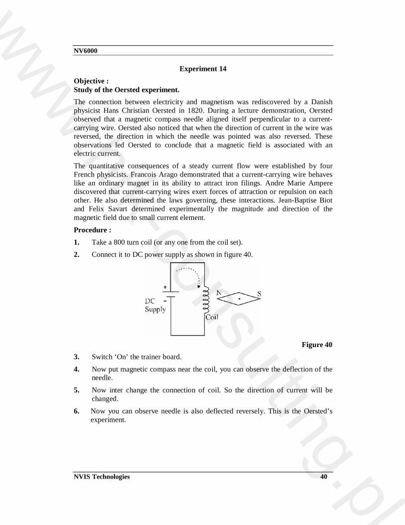
Procedure : 1. Take a 800 turn coil (or any one from the coil set). 2. Connect it to DC power supply as shown in figure 40.

Figure 40

3. Switch ‘On’ the trainer board.

4. Now put magnetic compass near the coil, you can observe the deflection of the needle.

5. Now inter change the connection of coil. So the direction of current will be changed.

6. Now you can observe needle is also deflected reversely. This is the Oersted’s experiment.


NV6000


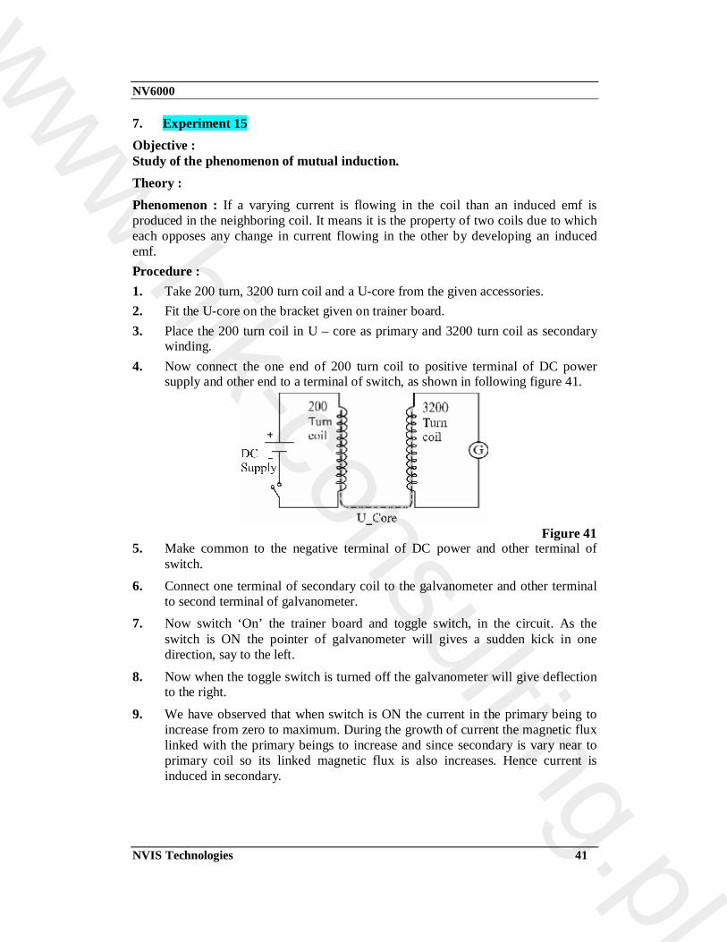
7. Experiment 15 Objective : Study of the phenomenon of mutual induction. Theory : Phenomenon : If a varying current is flowing in the coil than an induced emf is produced in the neighboring coil. It means it is the property of two coils due to which each opposes any change in current flowing in the other by developing an induced emf. Procedure : 1. Take 200 turn, 3200 turn coil and a U-core from the given accessories. 2. Fit the U-core on the bracket given on trainer board. 3. Place the 200 turn coil in U – core as primary and 3200 turn coil as secondary

winding. 4. Now connect the one end of 200 turn coil to positive terminal of DC power

supply and other end to a terminal of switch, as shown in following figure 41.

Figure 41

5. Make common to the negative terminal of DC power and other terminal of switch.

6. Connect one terminal of secondary coil to the galvanometer and other terminal to second terminal of galvanometer.

7. Now switch ‘On’ the trainer board and toggle switch, in the circuit. As the switch is ON the pointer of galvanometer will gives a sudden kick in one direction, say to the left.

8. Now when the toggle switch is turned off the galvanometer will give deflection to the right.

9. We have observed that when switch is ON the current in the primary being to increase from zero to maximum. During the growth of current the magnetic flux linked with the primary beings to increase and since secondary is vary near to primary coil so its linked magnetic flux is also increases. Hence current is induced in secondary.


NV6000


10. Now according to Lenz’s law the direction of current in secondary is such as to oppose the growth of power supply current in the primary, so the deflection of galvanometer is because of secondary induced current. When the switch is turned ‘Off’ the current in the primary coil beings to decrease towards zero. So the magnetic flux linked with primary and as well as secondary also decrease. Because of that an induced current flows in secondary. According to Lenz’s law the direction of current should be such as to oppose the decrease of current in the primary and this is possible only if the induced current flows in same direction as the power supply current in the primary. That is why the galvanometer gives deflection to the right direction at the time of break of circuit.


NV6000


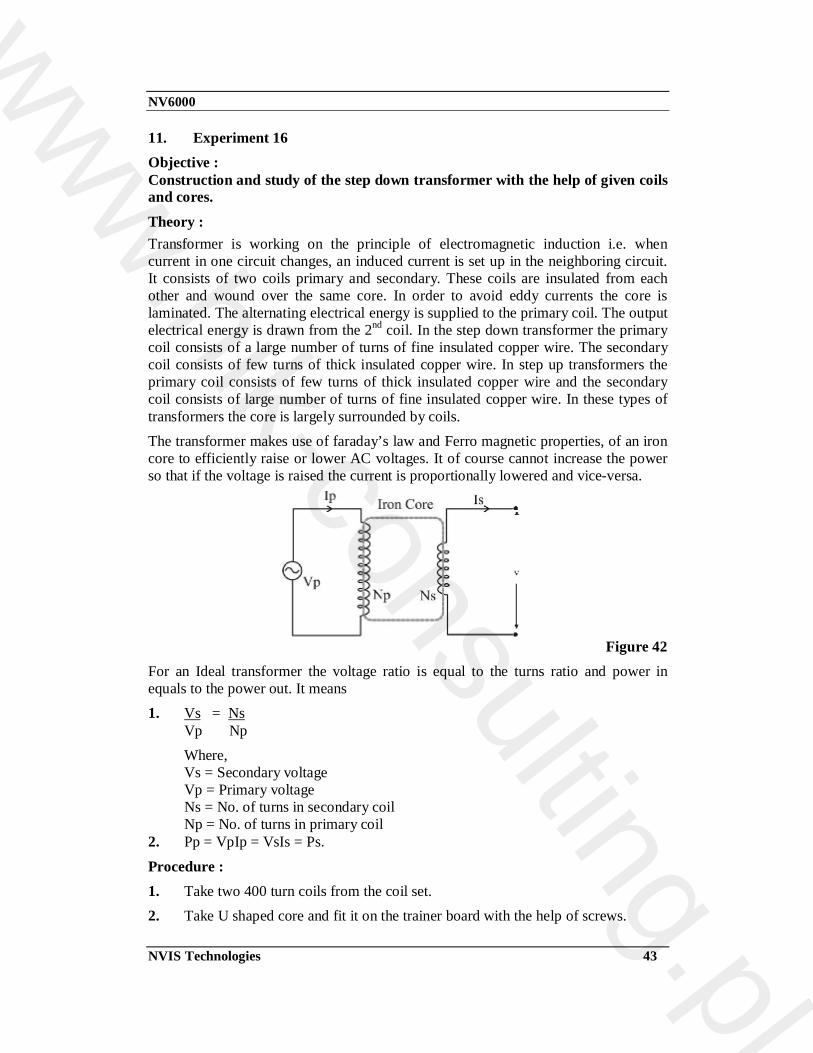
11. Experiment 16 Objective : Construction and study of the step down transformer with the help of given coils and cores. Theory : Transformer is working on the principle of electromagnetic induction i.e. when current in one circuit changes, an induced current is set up in the neighboring circuit. It consists of two coils primary and secondary. These coils are insulated from each other and wound over the same core. In order to avoid eddy currents the core is laminated. The alternating electrical energy is supplied to the primary coil. The output electrical energy is drawn from the 2nd coil. In the step down transformer the primary coil consists of a large number of turns of fine insulated copper wire. The secondary coil consists of few turns of thick insulated copper wire. In step up transformers the primary coil consists of few turns of thick insulated copper wire and the secondary coil consists of large number of turns of fine insulated copper wire. In these types of transformers the core is largely surrounded by coils. The transformer makes use of faraday’s law and Ferro magnetic properties, of an iron core to efficiently raise or lower AC voltages. It of course cannot increase the power so that if the voltage is raised the current is proportionally lowered and vice-versa.

Figure 42

For an Ideal transformer the voltage ratio is equal to the turns ratio and power in equals to the power out. It means 1. Vs = Ns

Vp Np Where, Vs = Secondary voltage Vp = Primary voltage Ns = No. of turns in secondary coil Np = No. of turns in primary coil

2. Pp = VpIp = VsIs = Ps.

Procedure : 1. Take two 400 turn coils from the coil set. 2. Take U shaped core and fit it on the trainer board with the help of screws.


NV6000


3. Now insert one 400 turn coil in U core as a primary coil and other as a secondary coil. Also put I shaped core on the U core to complete the flux linkages.

4. Connect primary coil to the DC power supply.

5. Measure the secondary voltage with the help of multimeter.

6. Observe the result there will be no output voltage.

7. Now change the power supply from DC to AC. 8. Now measure the secondary voltage in multimeter there will be some reading.

Note : These are not ideal transformers. Since coils are not coaxially wound on the same core the losses are more or the voltage transformation ratio is proportionately below the ideal values based on number of turns per coil. But effective quantitative investigation can be done with the help of this set upto 20% loss may be obtained from desire voltage.

9. Note the reading (ideally it should be same as input voltage because number of turns are same). Also note the percentage of losses. It will be helpful for further pairs of coils and for their calculations.

10. Now connect 200 turn coil in secondary and measure the voltage. You can observe the voltage is lowered.

11. In the same way you can connect any large number of coil as a primary and can record the results for different lower turns secondary coils in the table.

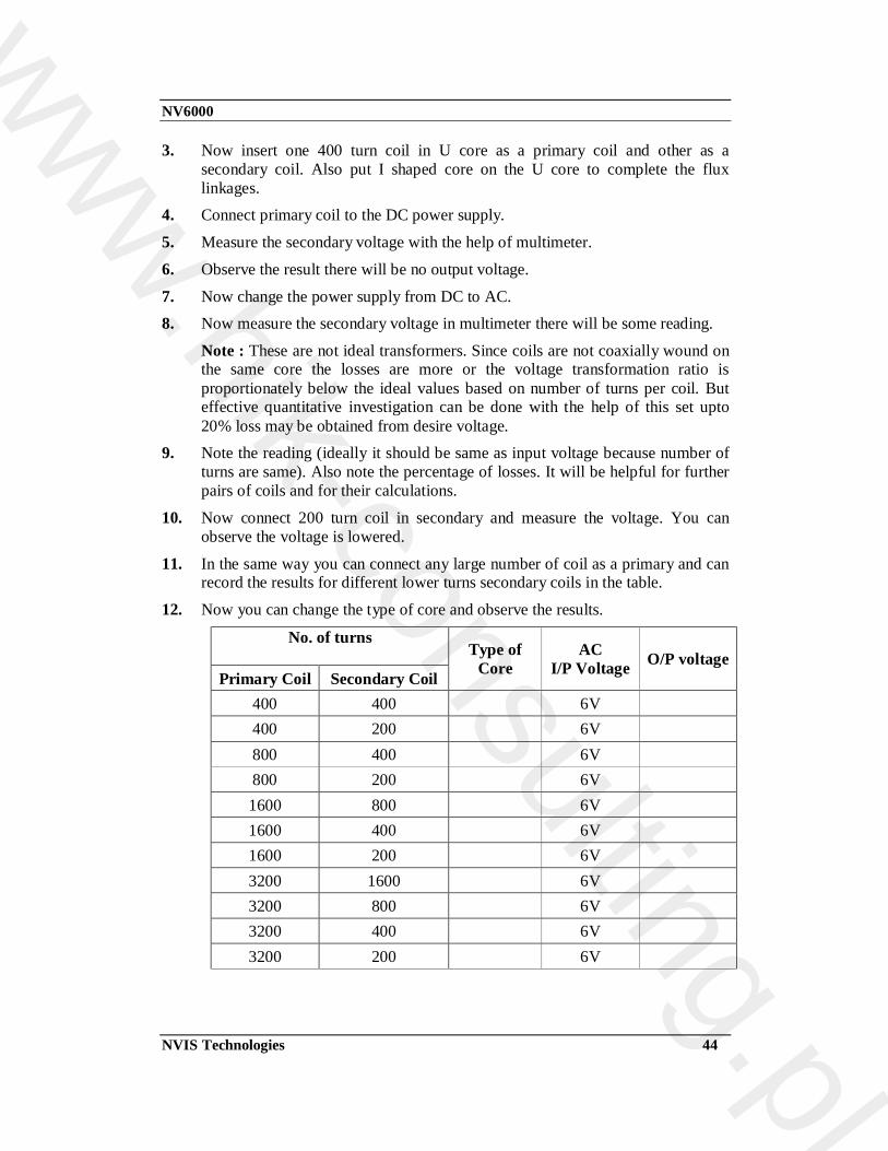
12. Now you can change the type of core and observe the results.

No. of turns

Primary Coil Secondary Coil

Type of Core

AC I/P Voltage O/P voltage

400 400 6V 400 200 6V 800 400 6V 800 200 6V 1600 800 6V 1600 400 6V 1600 200 6V 3200 1600 6V 3200 800 6V 3200 400 6V 3200 200 6V


NV6000


Experiment 17 Objective : Construction and study of the step up transformer. Procedure : 1. Repeat step 1 to 9 from the previous experiment of step down transformer. 2. Now connect 800 turn coil in the circuit as secondary coil. Observe the result,

the voltage is higher than that of input voltage 6V. 3. Now you can connect any combination of a lower turn primary coil and large

turns secondary coil. 4. Record the result in the given table.

5. Now observe the result by changing the core.

No. of turns

Type of Core

AC I/P Voltage O/P voltage

Primary Coil Secondary Coil 400 400 6V 400 800 6V 400 1600 6V 400 3200 6V 800 1600 6V 800 3200 6V

1600 3200 6V 200 400 6V 200 800 6V 200 1600 6V 200 3200 6V


NV6000


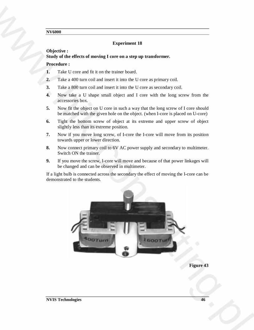
Experiment 18 Objective : Study of the effects of moving I core on a step up transformer. Procedure : 1. Take U core and fit it on the trainer board. 2. Take a 400 turn coil and insert it into the U core as primary coil.

3. Take a 800 turn coil and insert it into the U core as secondary coil. 4. Now take a U shape small object and I core with the long screw from the

accessories box. 5. Now fit the object on U core in such a way that the long screw of I core should

be matched with the given hole on the object. (when I-core is placed on U-core) 6. Tight the bottom screw of object at its extreme and upper screw of object

slightly less than its extreme position. 7. Now if you move long screw, of I-core the I-core will move from its position

towards upper or lower direction.

8. Now connect primary coil to 6V AC power supply and secondary to multimeter. Switch ON the trainer.

9. If you move the screw, I-core will move and because of that power linkages will be changed and can be observed in multimeter.

If a light bulb is connected across the secondary the effect of moving the I-core can be demonstrated to the students.

Figure 43


NV6000


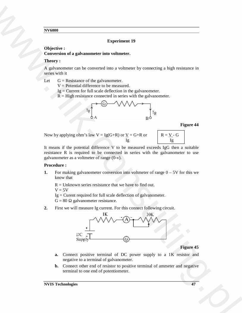
Experiment 19 Objective : Conversion of a galvanometer into voltmeter. Theory : A galvanometer can be converted into a voltmeter by connecting a high resistance in series with it

Let G = Resistance of the galvanometer. V = Potential difference to be measured. Ig = Current for full scale deflection in the galvanometer. R = High resistance connected in series with the galvanometer.

Figure 44

Now by applying ohm’s law V = Ig(G+R) or V = G+R or Ig It means if the potential difference V to be measured exceeds IgG then a suitable resistance R is required to be connected in series with the galvanometer to use galvanometer as a voltmeter of range (0-v).

Procedure : 1. For making galvanometer conversion into voltmeter of range 0 – 5V for this we

know that R = Unknown series resistance that we have to find out. V = 5V Ig = Curent required for full scale deflection of galvanometer. G = 80 Ω galvanometer resistance.

2. First we will measure Ig current. For this connect following circuit.

Figure 45

a. Connect positive terminal of DC power supply to a 1K resistor and negative to a terminal of galvanometer.

b. Connect other end of resistor to positive terminal of ammeter and negative terminal to one end of potentiometer.

R = V - G Ig


NV6000


c. Set the potentiometer fully clockwise direction. d. Connect other end of galvanometer and potentionmeter with each other.

3. Now as you switch ‘On’ the trainer board you can observe some deflection in galvanometer, now adjust the potentiometer such that to get full scale deflection of needle.

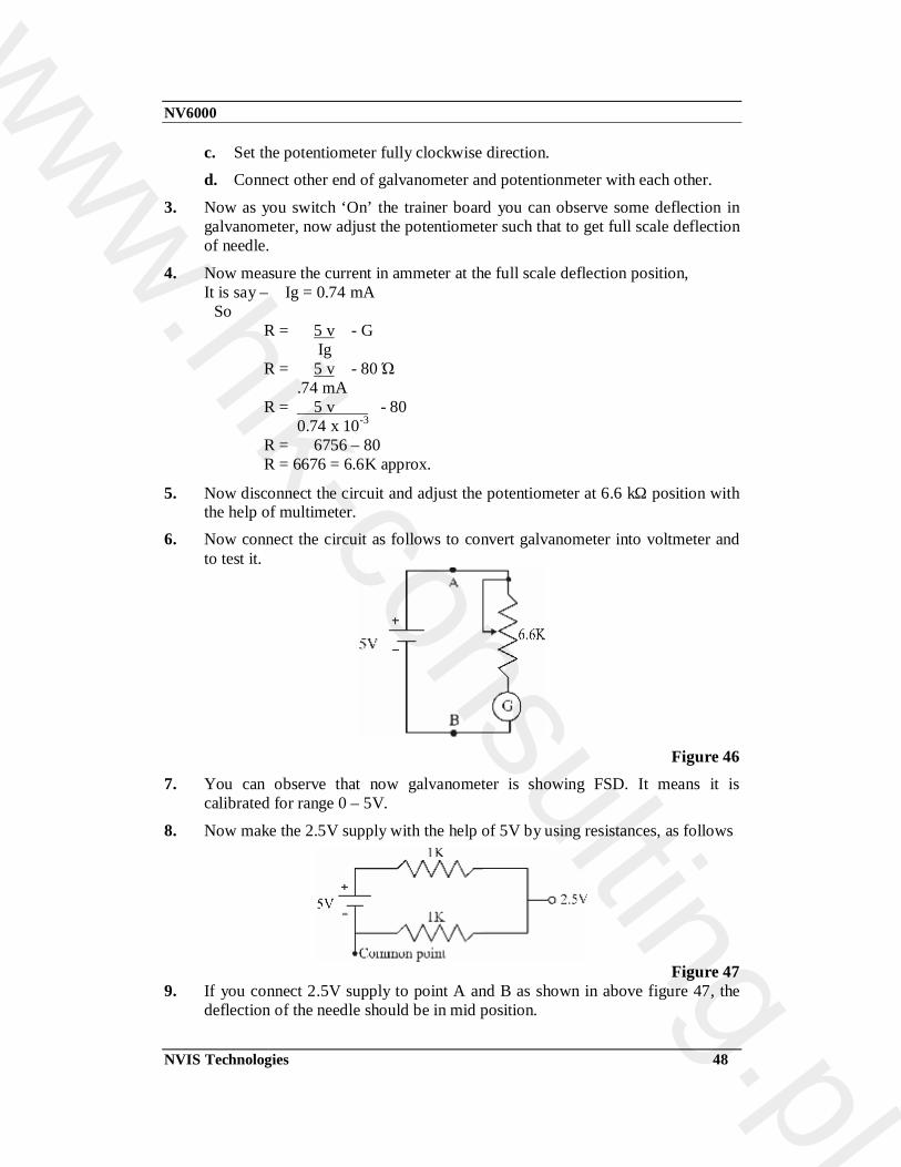
4. Now measure the current in ammeter at the full scale deflection position, It is say – Ig = 0.74 mA

So R = 5 v - G Ig R = 5 v - 80 Ώ .74 mA R = 5 v - 80 0.74 x 10-3

R = 6756 – 80 R = 6676 = 6.6K approx.

5. Now disconnect the circuit and adjust the potentiometer at 6.6 kΩ position with the help of multimeter.

6. Now connect the circuit as follows to convert galvanometer into voltmeter and to test it.

Figure 46

7. You can observe that now galvanometer is showing FSD. It means it is calibrated for range 0 – 5V.

8. Now make the 2.5V supply with the help of 5V by using resistances, as follows

Figure 47

9. If you connect 2.5V supply to point A and B as shown in above figure 47, the deflection of the needle should be in mid position.


NV6000


Experiment 20 Objective : Conversion of a galvanometer into ammeter. Theory : A galvanometer can be converted into ammeter by connecting parallel resistances of low value called shunt.

Figure 48

Potential difference across the galvanometer = IgG Potential difference across the shunt = (I-Ig) S Since both are connected in parallel so both should be equal (I-Ig)S = IgG S = Ig G

I – Ig Where

I = Unknown current that we have to measure Ig = Current required to galvanometer for FSD G = Galvanometer resistance S = Shunt resistance that we have connect in parallel to galvanometer

Procedure : For making galvanometer conversion into ammeter of range 0 – 50 mA 1. For this we know that

S = IgG I-Ig S = Unknown resistance that we have to find out. Ig = We have already calculated it, in previous experiment = 0.74mA (approx.) I = Unknown current to be measured. G = 80 Ω Now S = 0.74mA x 80 50mA – 0.74mA S = 0.74 x 10-3 x 80 (50 – 0.74) x 10-3

S = 59.2 /49.26 S = 1.2 Ω


NV6000


2. Now adjust the potentiometer 25E given on trainer board to the vale of 1.2 Ω with the help of multimeter and connect it to the parallel of galvanometer as shown in following figure 49.

3. Now if you want to have 50 mA current in the circuit of supply 5V than you have to connect 100 Ω resistance accesses it from ohm’s law.

4. Adjust the potentiometer (10K) for value = 100Ω. 5. Now as you switch ‘On’ the trainer board you can observe the needle is having

full scale deflection. It means now the galvanometer is calibrated for range 0-50 mA.

Figure 49

Now if you increase the resistance from 100 Ώ to 200 Ώ (Pot 10 K) then the current will be just half of the previous case i.e., 25mA and you can observe the pointer of the galvanometer is deflected upto the mid position.


NV6000


Experiment 21 Objective : Study of the Hysteresis curve. Equipments Needed : 1. Function Generator 2. CRO

3. 100K ohm and 10 ohm resistance 4. E, I core

5. 400 and 3200 Turn coils 6. Patch cords etc.

Theory : A great deal of information can be learned about the magnetic properties of a material by studying its hysteresis loop. A hysteresis loop shows the relationship between the induced magnetic flux density (B) and the magnetizing force (H). It is often referred to as the B-H loop. An example hysteresis loop is shown below.

Figure 50

The loop is generated by measuring the magnetic flux of a ferromagnetic material while the magnetizing force is changed. A ferromagnetic material that has never been previously magnetized or has been thoroughly demagnetized will follow the dashed line as H is increased. As the line demonstrates, the greater the amount of current applied (H+), the stronger the magnetic field in the component (B+). At point "a" almost all of the magnetic domains are aligned and an additional increase in the magnetizing force will produce very little increase in magnetic flux. The material has reached the point of magnetic saturation. When H is reduced to zero, the curve will move from point "a" to point "b." At this point, it can be seen that some magnetic flux remains in the material


NV6000


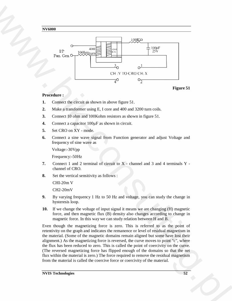
Figure 51

Procedure : 1. Connect the circuit as shown in above figure 51. 2. Make a transformer using E, I core and 400 and 3200 turn coils.

3. Connect 10 ohm and 100Kohm resistors as shown in figure 51.

4. Connect a capacitor 100μF as shown in circuit.

5. Set CRO on XY - mode. 6. Connect a sine wave signal from Function generator and adjust Voltage and

frequency of sine wave as Voltage:-30Vpp

Frequency:-50Hz 7. Connect 1 and 2 terminal of circuit to X - channel and 3 and 4 terminals Y -

channel of CRO. 8. Set the vertical sensitivity as follows :

CHI-20m V CH2-20mV

9. By varying frequency 1 Hz to 50 Hz and voltage, you can study the change in hysteresis loop.

10. If we change the voltage of input signal it means we are changing (H) magnetic force, and then magnetic flux (B) density also changes according to change in magnetic force. In this way we can study relation between H and B.

Even though the magnetizing force is zero. This is referred to as the point of retentivity on the graph and indicates the remanence or level of residual magnetism in the material. (Some of the magnetic domains remain aligned but some have lost their alignment.) As the magnetizing force is reversed, the curve moves to point "c", where the flux has been reduced to zero. This is called the point of coercivity on the curve. (The reversed magnetizing force has flipped enough of the domains so that the net flux within the material is zero.) The force required to remove the residual magnetism from the material is called the coercive force or coercivity of the material.


NV6000


As the magnetizing force is increased in the negative direction, the material will again become magnetically saturated but in the opposite direction (point "d"). Reducing H to zero brings the curve to point "e." It will have a level of residual magnetism equal to that achieved in the other direction. Increasing H back in the positive direction will return B to zero. Notice that the curve did not return to the origin of the graph because some force is required to remove the residual magnetism. The curve will take a different path from point “F” back to the saturation point where it with complete the loop.

From the hysteresis loop, a number of primary magnetic properties of a material can be determined.

1. Retentivity : A measure of the residual flux density corresponding to the saturation induction of a magnetic material. In other words, it is a material's ability to retain a certain amount of residual magnetic field when the magnetizing force is removed after achieving saturation. (The value of B at point b on the hysteresis curve.)

2. Residual Magnetism or Residual Flux : the magnetic flux density that remains in a material when the magnetizing force is zero. Note that residual magnetism and retentivity are the same when the material has been magnetized to the saturation point. However, the level of residual magnetism may be lower than the retentivity value when the magnetizing force did not reach the saturation level.

3. Coercive Force : The amount of reverse magnetic field which must be applied to a magnetic material to make the magnetic flux return to zero. (The value of H at point c on the hysteresis curve.)

4. Permeability, µ : A property of a material that describes the ease with which a magnetic flux is established in the component.

5. Reluctance - Is the opposition that a ferromagnetic material shows to the establishment of a magnetic field. Reluctance is analogous to the resistance in an electrical circuit.


NV6000


Warranty 1) We guarantee the product against all manufacturing defects for 24 months from

the date of sale by us or through our dealers. Consumables like dry cell etc. are not covered under warranty.

2) The guarantee will become void, if

a) The product is not operated as per the instruction given in the operating manual.

b) The agreed payment terms and other conditions of sale are not followed.

c) The customer resells the instrument to another party. d) Any attempt is made to service and modify the instrument.

3) The non-working of the product is to be communicated to us immediately giving full details of the complaints and defects noticed specifically mentioning the type, serial number of the product and date of purchase etc.

4) The repair work will be carried out, provided the product is dispatched securely packed and insured. The transportation charges shall be borne by the customer.


NV6000


List of Accessories 1. Mains cord.................................................................................................1 No.

2. Parch cord 2mm to 2mm (10”) .............................................................. 10 Nos. 3. Coils 200, 800, 1600, 3200 turns.............................................................. 1 each

4. 400 turn coil............................................................................................. 2 Nos. 5. Bar magnet ................................................................................................1 No.

6. Magnetic compass......................................................................................1 No. 7. U, E, I core .............................................................................................. 1 each

8. I core with long screw................................................................................1 No. 9. Pieces of soft iron .................................................................................... 5 Nos. 10. Component box

Resistances : 100 Ω .............................................................................................. 15 Nos. 200 Ω .............................................................................................. 10 Nos. 220 Ω ............................................................................................... 10 Nos. 332 Ω .............................................................................................. 10 Nos. 1KΩ ................................................................................................. 10 Nos. 100 KΩ............................................................................................. 10 Nos. 220 KΩ............................................................................................. 10 Nos. 5 KΩ .................................................................................................. 2 Nos.

11. Potentiometer 10 K ....................................................................................1 No.

12. Electrolytic capacitor 100µf .................................................................... 2 Nos.

13. Metalized poly. Capacitor 0.1µf ............................................................... 2 Nos. 14. Diode (1N4007)....................................................................................... 5 Nos.

15. Transistor (BC547) .................................................................................. 5 Nos.

16. Multimeter ................................................................................................1 No.


Electricity Lab NV6000 - Specjalizowane przyrządy i ... · Electricity Lab NV6000 ... Conversion...

Documents

Transcript of Electricity Lab NV6000 - Specjalizowane przyrządy i ... · Electricity Lab NV6000 ... Conversion...