Electricity Diversity Profiles for Energy Simulation of Office Buildings (1093-RP) David E. Claridge, Ph.D., P.E. Bass Abushakra, Ph.D. Jeff S. Haberl, Ph.D., P.E. Member ASHRAE Member ASHRAE Member ASHRAE Atch Sreshthaputra Student Member ASHRAE

ABSTRACT This paper presents diversity factors recommended for use in energy simulation programs that require

the input of hourly usage of electricity for lighting, and receptacle loads relative to the installed lighting/equipment capacity. Typical weekday and weekend profiles are presented for small, medium and large office buildings. The diversity profiles were developed from year-long records from 46 channels of hourly or 15-minute data recorded in 32 buildings. This data was acquired and analyzed under ASHRAE Research Project 1093-RP. In addition to the typical profiles developed, weekday and weekend profiles are presented for each of the 46 channels of data analyzed.

INTRODUCTION In most office buildings, internal heat gains from people, plug loads and lighting are significant

contributors to the cooling load and hence are very important for energy calculations. Hourly energy simulation programs typically require the input of representative hourly values of the electrical consumption of lights and plug loads. The heat gains from these sources deviate from their peak values due to people entering and leaving the building who switch lights and equipment on and off. Some equipment such as computers and copiers automatically switches to "standby" or "energy saving"' modes when unused for a period of time during the day. This variability in operation of office equipment and lighting is typically treated by inputting the peak consumption of lighting and plug loads and then using different sets of 24-hour “diversity factors” for week-days, week-ends, and any other set(s) of important daily variations. The diversity factors are numbers between zero and one that are used to multiply the peak consumption that has been input. Sets of diversity factors given in the users manuals of individual simulation programs or estimated from engineering experience are normally used in simulation.

The goal of ASHRAE 1093-RP was to compile a library of schedules and diversity factors based on

measured electricity consumption data for use in energy simulations and peak cooling load calculations in office buildings. This research project derived multiple sets of diversity factors from measured data in 32 office buildings. As part of the research, the methods reported in the literature for generating load profiles were carefully reviewed, and a methodology suitable for use with one year of hourly profiles was developed and implemented in a spreadsheet. The project also developed a procedure for estimating diversity profiles for loads due to occupants that is based on the diversity profiles for lights and plug loads (Abushakra and Claridge 2001).

This paper presents typical weekday and weekend diversity profiles for weather-independent

electricity use suitable for use in energy simulations of different categories of office buildings. Typical profiles are presented for lighting, plug loads, combined lighting and plug loads, and for whole-building electricity use including fans and pumps. A review of the literature on diversity profiles and methods for determining day types is given in Abushakra et al. (2004). A detailed description of the methodology employed in the project is presented in the project’s final report (Abushakra et al. (2002), which also includes:

• the description of a spreadsheet that can be used to generate similar profiles from measured hourly data for any building.

• a library of the schedules and diversity factors for all 32 buildings analyzed in this project, presented in tabular form, for cases where specialized diversity factors may be more suitable.

• input files for DOE-2, BLAST, and EnergyPlus simulation programs. The data used to develop the diversity profiles presented in this paper is described first, followed by a

brief description of the method used to derive the profiles from the data. The paper concludes with presentation and discussion of the diversity profiles.

DATA USED TO DEVELOP THE PROFILES An extensive search was conducted to locate and identify databases of monitored data in the U.S. and

Europe that contained suitable data for this project. Major databases reviewed included ASHRAE FIND (ASHRAE 1995), EPRI-CEED (CEED 1995, EPRI 1999), ELCAP (Gilman et al. 1990), Lawrence Berkeley National Laboratory and the Energy Systems Laboratory (Turner et al., 2000). The literature was reviewed to see if it revealed additional potential sources of data. In addition, 10 leading scholars, researchers, and energy consultants in the U.S. and 20 in Europe were contacted through e-mail, fax, or phone calls in an attempt to identify additional sources of data.

This search revealed the existence of data for several hundred buildings. However, much of this data

included heating and/or cooling consumption which made it unsuitable for use in this study. Other data which would have been suitable could not be obtained at a cost within the resources of this study. The project investigators with the concurrence of the project monitoring committee eventually selected the data available from the Lawrence Berkeley National Laboratory (LBNL) for the Energy-Edge program, and that available at the Energy Systems Laboratory. This Energy Systems Laboratory (ESL) data base contains data from the buildings in the Texas LoanSTAR program and other buildings around the country monitored by the laboratory. This provided an initial group of over 200 buildings that was eventually reduced to the 46 data sets from 32 office buildings that are summarized in Table 1.

The data consisted of hourly monitored lighting and receptacles loads and other weather-independent

electricity consumption from various office buildings around the country. The LBNL data included lighting and receptacles loads separately, whereas most of the ESL data consisted of separate channels for Whole-Building Electric (WBE) and Motor Control Center (MCC) loads. Cooling loads in most of the buildings monitored by the ESL were separately monitored as Btu loads, and therefore were not included in the Whole-Building Electric data. The motor control centers included in the MCC data typically provide electricity to most of the air handlers and pumps in the building. Hence the “Lighting and Receptacles” loads - as a sum - were obtained as the difference between the WBE and MCC loads for these buildings.

The buildings shown have been separated into three categories based on the classification scheme used

by the Commercial Buildings Energy Consumption Survey (CBECS 1997a and b) conducted by the Energy Information Administration of the U.S. Department of Energy. This survey groups buildings based on floor area as: (1) Small (1,001 - 10,000 ft2), (2) Medium (10,001 - 100,000 ft2), and (3) Large (>100,000 ft2). The first column of Table 1 indicates this size category by S, M or L.

The second column of the table is a site identification number used in the study that combines the

location (state), size category, and an arbitrary number assigned to that site. This number is also used to identify the profiles from this building in figures that appear later in the paper. Sites with the same ID number except for the last letter correspond to different channels of data from the same building with "a" corresponding to lighting data, "b" to receptacle data and "c" to the sum of the lighting and receptacle data. The next column gives the city and state where the building is located and the fourth column gives the building conditioned area in square feet.

The fifth column indicates the type of data collected as follows: • WBE: whole-building electricity use including fans and pumps, but not including heating or

cooling consumption;

• WBE-MCC: data representative of weather-independent consumption calculated by subtracting motor control center consumption from whole-building electricity consumption;

• WBE-MCC-AHU: data representative of weather-independent consumption calculated by subtracting motor control center and air handler consumption from whole-building electricity consumption;

• WBE-MCC-Chill: data representative of weather-independent consumption calculated by subtracting motor control center and chiller consumption from whole-building electricity consumption;

• LIGHT: sub-metered lighting consumption; • RECEPT: sub-metered 120 VAC receptacle consumption; and • LIGHT+RECEPT: the sum of the previous two data streams for an individual building. It should be noted that the categories WBE-MCC, WBE-MCC-AHU, and WBE-MCC-Chill were

applied only to buildings after determining that any known weather-dependent consumption in the building was metered in the categories that were subtracted.

The sixth column shows the maximum hourly load present in each one-year data set expressed in W/

ft2. and the seventh column indicates the data source. The eighth column gives the annual energy use index (EUI) for the data set based on 52 weeks of weekday-weekend energy use profiles as presented in this paper and expressed in kWh/(ft2-yr.). The next two columns provide “weekday” daily totals of two diversity factors which are summarized in Table 2 and discussed in the next section. The final column gives the start date for the one-year data set.

Each dataset was inspected for obvious outliers that were removed prior to processing. In several of

the ESL sites, data removals included periods that exhibited slight weather dependency. Holidays that appeared on weekdays were also removed. Several of the LBNL sites contained synthetic or imputed data that were also removed. In each site all data removals are clearly indicated in the project final report (Abushakra et al. 2002). All data used in this project represents measured data. Gaps were left as-is in the data sets (i.e., no data-filling nor inputing of data was performed).

METHODOLOGY USED TO DERIVE DIVERSITY FACTORS After performing the data quality checks, the maximum consumption value was determined for each

data channel and expressed in W/ft2. This maximum value is used to normalize all the hourly data from each site so that the data can be expressed in terms of a diversity factor with a value in the range 0 – 1 that is compatible with the DOE-2, BLAST and EnergyPlus input files. In each program, the hourly demand is calculated by multiplying the diversity factor for each hour by the maximum consumption.

The data were then sorted into weekday and weekend data. Then, for each hour of the day, the 10th,

25th, 50th, 75th, 90th percentile values, the mean and the mean + one standard deviation were calculated and tabulated. This was separately performed for the weekday data and for the weekend data. All values were then normalized to values between 0 to 1, by dividing by the absolute maximum value in the dataset to obtain the weekday and weekend diversity factors in tabular and graphical formats. A visual inspection of the load shapes was then used to determine if any of the profiles were inconsistent and/or contained data that needed to be eliminated (i.e., known holidays, shutdowns, etc.). For example, an unusually low minimum profile in the weekday group (which looks very much like a weekend profile) usually indicated a holiday, or a weekday profile in the weekend group usually indicated a special event. In most cases the data associated with these low or high values were removed from the dataset and the diversity factors recalculated. The dates of the removed data were recorded for each site.

The median or 50th percentile values are presented in this paper for use as the diversity factors in

simulation input files. The percentile analysis was adopted instead of the more widely used mean and standard deviation approach (e.g. Noren and Pyrko 1997, and 1998a and b), because the lighting and receptacle loads present in the office buildings studied for this project often exhibited a multi-modal distribution (where the frequency curve exhibits more than one maximum) rather than a normal distribution

as required for mean and standard deviation analysis. Furthermore, many of the office buildings had significant outliers that also influenced the standard deviation and the mean.

Therefore the median was chosen for the diversity factors because it is less affected by outliers. The 10th, 25th, 75th, and 90th percentiles are also more robust than the standard deviation when outliers are present in a dataset. Percentile analysis is also more robust with datasets that tend to have a multimodal distribution (where the frequency curve exhibits few maxima).

The primary purpose of a diversity profile for energy simulation is to represent the hourly distribution

of the energy use. However, the degree to which the use of the peak measured consumption for a building multiplied by the diversity profile represents typical daily consumption was investigated by determining typical daily consumption in two ways. The first was by simply computing typical daily weekday consumption; when the typical daily weekday consumption is normalized to the maximum hourly consumption in the dataset, the resulting value is called "Daily Sum". The second was by multiplying the hourly diversity profile values by the peak consumption; the summation of the 24 values of the hourly diversity profile is called Daily from Hourly or “DFH”. In both cases, these are dimensionless 24-hour totals of diversity factors. These values were calculated for the profiles determined for all 46 datasets and are summarized in Table 2. The three columns contain the average, maximum and minimum of the quantity shown in each row when all 46 datasets are considered. In general, the averages are most important for the current comparison, but the maximum and minimum values are given as well to show the range of values encountered. The average value of the DFH sum of diversity factors for weekdays is 0.24% smaller than the same sum based on daily totals. This leads us to conclude that the profiles accurately represent typical days of operation.

To further test the procedure, one year of hourly predicted lighting and receptacle loads (kWh/h) was

calculated for building TXL004, which had no missing or bad data, using the 1093-RP typical load shapes procedure. The predicted year was constructed by creating 52 weeks of 5 weekday load shapes and 2 weekend load shapes, filling in the known holidays with weekend load shapes, and then multiplying the sum of these diversity factors by the peak measured consumption. The total yearly predicted consumption was 888,739 kWh while the total yearly measured consumption was 885,224 kWh -- a bias error of 0.397% which suggests that the procedure developed represents the measured data with accuracy at least as great as that of other simulation inputs.

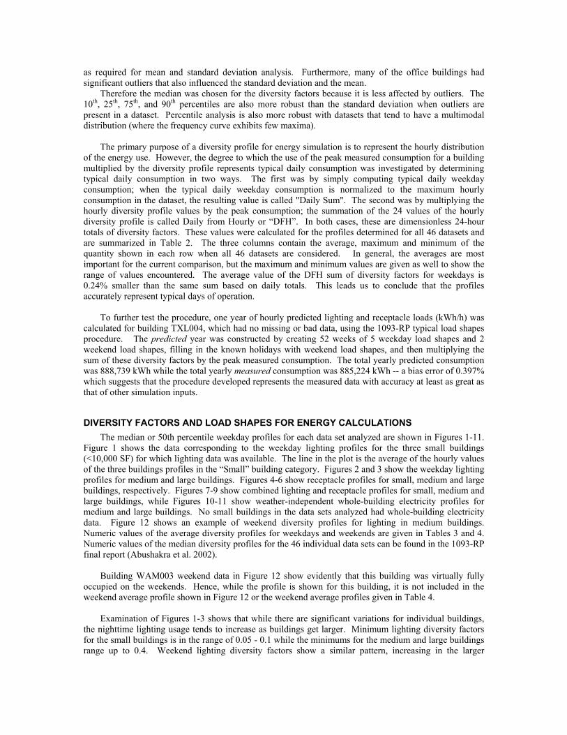
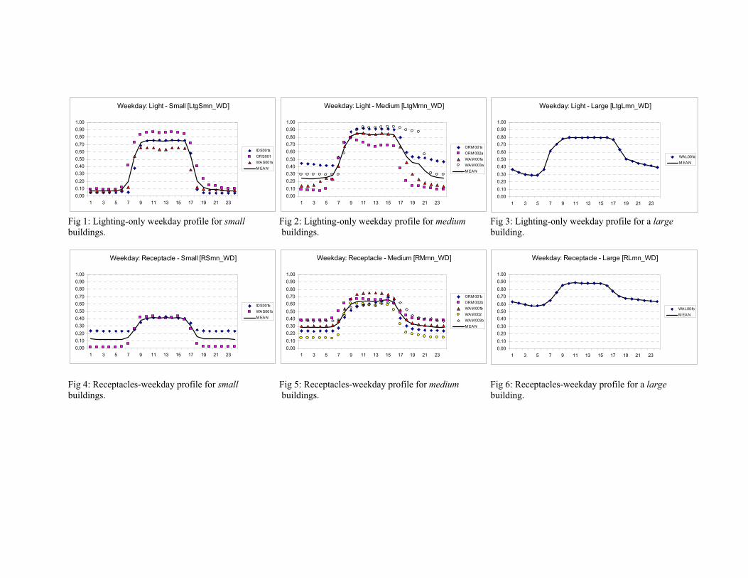
DIVERSITY FACTORS AND LOAD SHAPES FOR ENERGY CALCULATIONS The median or 50th percentile weekday profiles for each data set analyzed are shown in Figures 1-11.

Figure 1 shows the data corresponding to the weekday lighting profiles for the three small buildings (<10,000 SF) for which lighting data was available. The line in the plot is the average of the hourly values of the three buildings profiles in the “Small” building category. Figures 2 and 3 show the weekday lighting profiles for medium and large buildings. Figures 4-6 show receptacle profiles for small, medium and large buildings, respectively. Figures 7-9 show combined lighting and receptacle profiles for small, medium and large buildings, while Figures 10-11 show weather-independent whole-building electricity profiles for medium and large buildings. No small buildings in the data sets analyzed had whole-building electricity data. Figure 12 shows an example of weekend diversity profiles for lighting in medium buildings. Numeric values of the average diversity profiles for weekdays and weekends are given in Tables 3 and 4. Numeric values of the median diversity profiles for the 46 individual data sets can be found in the 1093-RP final report (Abushakra et al. 2002).

Building WAM003 weekend data in Figure 12 show evidently that this building was virtually fully

occupied on the weekends. Hence, while the profile is shown for this building, it is not included in the weekend average profile shown in Figure 12 or the weekend average profiles given in Table 4.

Examination of Figures 1-3 shows that while there are significant variations for individual buildings,

the nighttime lighting usage tends to increase as buildings get larger. Minimum lighting diversity factors for the small buildings is in the range of 0.05 - 0.1 while the minimums for the medium and large buildings range up to 0.4. Weekend lighting diversity factors show a similar pattern, increasing in the larger

buildings. Building WAM003 seems to be almost fully occupied on weekends, as noted, with its weekend peak diversity factor only a few percentage points lower than its weekday peak.

Receptacle diversity factors differ substantially from the lighting diversity factors as shown in Figures

4-6. They do show the same tendency to increase with building size, but they are much more "compressed" with the range between the minimum and maximum weekday receptacle diversity factors being about half the range for the lighting diversity factors.

The combined lights and receptacle diversity factors of Figures 7-9 and the weather-independent WBE

diversity factors of Figures 10-11 are quite similar, as might be expected. The buildings shown offer considerable variation, but the average profiles for these two groups are remarkably similar, suggesting that the averages are quite typical.

CONCLUSIONS Diversity factors were developed for year-long hourly record of 46 channels in 32 office buildings.

These diversity factors are composed of the hourly median or 50th percentile from the buildings in each category (i.e., small, medium, and large). The median or 50th percentile profiles shown in Figures 1-12 and Tables 3 and 4 are recommended as appropriate for use in energy simulations. If the users have specific knowledge of schedules for the building they wish to simulate that differ from those shown, they can modify the 1093-RP profiles accordingly. This would be particularly true for weekend schedules. Some buildings show no weekend use, while others such as WAM003 appear to be almost fully occupied on weekends. The user may also choose to use the schedule for a particular building whose usage pattern resembles that anticipated for the building being simulated.

ACKNOWLEDGEMENTS The authors gratefully acknowledge the financial support of ASHRAE under Research Project 1093 in

the performance of this work. The authors are also grateful to the Project Monitoring Subcommittee members who have helped to guide the project and have provided useful comments and reviews of the work performed, including: Prof. Agami Reddy (PMSC Chair), Mr. Joe Huang, Prof. Bill Bahnfleth, and Ms. Suzanne Leviseur. This project would not have been possible without the support that was provided by the following persons and/or the agencies or companies for which they work: Ms. Theresa Sifuentes, Mr. Felix Lopez, and Mr. Dub Taylor at the Texas State Energy Conservation Office (SECO) who authorized the use of the LoanSTAR database; Ms. Mary Ann Piette at Lawrence Berkeley National Laboratory who authorized the use of Energy Edge Database and Ms. Satkartar Khalsa and Mr. Bruce Nordman who so speedily provided the data.

REFERENCES Abushakra, B., and D.E. Claridge. 2001. Accounting for the Occupancy Variable in Inverse Building

Energy Baselining Models. Proceedings of the International Conference for Enhanced Building Operations (ICEBO), Austin, Texas, July.

Abushakra, B., Sreshthaputra, A., Haberl, J.S., and D.E. Claridge. 2002. Compilation of Diversity Factors and Schedules for Energy and Cooling Load Calculations (ASHRAE Research Project 1093-RP Final Report). Energy Systems Laboratory Technical Report, ESL-TR-01/04-01, Department of Mechanical Engineering, Texas A&M University, February.

Abushakra, Bass, Haberl, Jeff and Claridge, David E., 2004. Overview of Existing Literature on Diversity Factors and Schedules for Energy and Cooling Load Calculations (1093-RP). ASHRAE Transactions.

ASHRAE 1995. ASHRAE FIND, An inventory of Measured Energy-use databases (a diskette and a user manual). American Society of Heating, Refrigeration and Air-Conditioning Engineers, Atlanta, Georgia.

CBECS 1997-a. Commercial buildings characteristics 1995. Commercial Buildings Energy Consumption Survey (CBECS), Energy Information Administration (EIA), Office of Energy Markets and End Use, USDOE, August 1997.

CBECS 1997-b. Commercial Buildings Energy Consumption and Expenditures 1995. Commercial Buildings Energy Consumption Survey (CBECS), Energy Information Administration (EIA), Office of Energy Markets and End Use, USDOE, 1997.

CEED 1995. Leveraging limited data resources: Developing commercial end-use information: BC Hydro case study. Technical Report. EPRI's Center for Electric End-Use Data (CEED). Portland, Oregon.

EPRI 1999. EPRI's Southeast Data Exchange. Information obtained from EPRI-CEED website. Center for Electric End-Use Data (CEED). Portland, Oregon.

Gillman, R., R.D. Sands, and G.L. Robert. 1990. Observations on residential and commercial load shapes during a cold snap. Proceedings of the 1990 ACEEE Summer Study on Energy Efficiency in Buildings, pp. 10.81-10.89.

Noren, C. 1997. Typical load shapes for six categories of Swedish commercial buildings. Technical Report, Lund Institute of Technology, Department of Heat and Power Engineering, Division of Energy Economics and Planning, Lund, Sweden.

Noren, C., and Pyrko, J. 1998a. Using multiple Regression analysis to develop electricity consumption indicators for public schools. Proceedings of the 1998 ACEEE Summer Study on Energy Efficiency in Buildings, pp. 3.255-3.266.

Noren, C., and Pyrko, J. 1998b. Typical load shapes for Swedish schools and hotels. Energy and Buildings. Volume 28, Number 3, 1998, pp.145-157.

Turner, W.D., Claridge, D.E., O'Neal, D.L., Haberl, J., Heffington, W., Taylor, D., and Sifuentes, T., 2000. "Program Overview: The Texas LoanSTAR Program: 1989-1999, a 10-Year Experience," Proc. of the 12th Symposium on Improving Building Systems in Hot and Humid Climates, San Antonio, TX, May 15-17, pp. 216-225.

TABLE 1 Summary Listing of the Data Sets Used to Develop the Diversity Profiles for 1093-RP

Category Site ID. Location Building Area (ft2) Data Type Max Load (W/ ft2)

Source EUI (kWh/ft2yr)

Weekday Daily Sum

Weekday DFH

Start Date

L DCL001 Washington D.C 1,200,000 WBE 3.93 ESL 19.99 16.09 16.26 1/1/94 S IDS001a Idaho Falls, ID 5,300 LIGHT 1.46 LBNL 3.19 7.92 7.63 1/1/89 S IDS001b Idaho Falls, ID 5,300 RECEPT 0.45 LBNL 1.00 7.22 7.16 1/1/89 S IDS001c Idaho Falls, ID 5,300 LIGHT+RECEPT 1.72 LBNL 4.20 8.67 8.43 1/1/89 L MNL001 Minneapolis, MN 200,829 WBE 0.83 ESL 4.27 15.69 15.39 1/1/98 L MNL002 Minneapolis, MN 281,850 WBE 0.59 ESL 2.87 14.47 14.47 1/1/98 L MNL003 Minneapolis, MN 366,805 WBE 0.58 ESL 2.96 15.21 15.18 1/1/98 L MNL004 Minneapolis, MN 317,286 WBE 1.09 ESL 7.40 19.38 19.41 1/1/98 M MNM002 Minneapolis, MN 87,664 WBE 0.52 ESL 2.69 15.76 15.83 3/1/96 L MTL001 Butte, MT 100,000 WBE 1.13 ESL 4.19 12.65 12.54 7/1/98 M ORM001a Portland, OR 79,700 LIGHT 1.15 LBNL 5.58 15.33 15.51 1/1/91 M ORM001b Portland, OR 79,700 RECEPT 0.6 LBNL 1.79 9.38 9.23 1/1/91 M ORM001b Portland, OR 79,700 LIGHT+RECEPT 1.69 LBNL 7.36 13.67 13.84 1/1/91 M ORM002a Eugene, OR 24,800 LIGHT 1.16 LBNL 3.07 9.26 8.81 1/1/91 M ORM002b Eugene, OR 24,800 RECEPT 0.66 LBNL 2.68 12.00 11.91 1/1/91 M ORM002c Eugene, OR 24,800 LIGHT+RECEPT 1.65 LBNL 5.75 11.35 11.00 1/1/91 S ORS001 Portland, OR 8,500 LIGHT 1.34 LBNL 4.28 10.62 10.49 1/1/88 L TXL001 Dallas, TX 473,800 WBE-MCC 2.51 ESL 10.61 12.93 12.92 1/1/95 L TXL002 Austin, TX 169,746 WBE-MCC 4.36 ESL 24.73 16.17 16.33 1/1/97 L TXL003 Austin, TX 102,000 WBE-MCC 3.54 ESL 20.05 17.14 17.11 1/1/96 L TXL004 Austin, TX 120,000 WBE-MCC 1.83 ESL 7.59 13.36 13.38 1/1/97 L TXL005 Austin, TX 491,000 WBE-MCC 3.13 ESL 16.46 15.73 15.80 1/1/97 L TXL006 Austin, TX 308,080 WBE-MCC-AHU 5.17 ESL 33.79 19.06 19.06 1/1/97 L TXL007 Austin, TX 151,620 WBE 2.76 ESL 15.95 17.40 17.35 1/1/98 L TXL008 Austin, TX 121,654 WBE 1.75 ESL 12.32 20.03 20.08 1/1/98 L TXL010 Bryan, TX 100,000 WBE-MCC 3.59 ESL 19.70 15.21 15.17 7/1/98 L TXL011 Austin, TX 282,499 WBE 3.39 ESL 21.17 17.94 17.99 7/1/97 L TXL012 Austin, TX 182,961 WBE 5.39 ESL 30.18 16.12 16.14 1/1/93 M TXM001 Austin, TX 80,000 WBE-MCC 5.22 ESL 34.42 19.15 19.15 1/1/94 M TXM002 Austin, TX 62,000 WBE-MCC-Chill 2.21 ESL 11.63 15.99 15.99 1/1/93 M TXM003 Austin, TX 97,030 WBE - Chill 3.76 ESL 13.49 11.68 11.91 1/1/96 M TXM004 Austin, TX 72,737 WBE 2.22 ESL 11.64 15.23 15.16 1/1/98 M TXM005 Dallas, TX 42,385 WBE 3.50 ESL 14.94 13.40 13.35 1/1/98 L WAL001a Bellevue, WA 389,000 LIGHT 1.34 LBNL 6.05 13.82 13.72 1/1/91 L WAL001b Bellevue, WA 389,000 RECEPT 0.40 LBNL 2.41 17.41 17.44 1/1/91 L WAL001c Bellevue, WA 389,000 LIGHT+RECEPT 1.71 LBNL 8.44 14.80 14.76 1/1/91 L WAM001a Bellevue, WA 25,100 LIGHT 0.77 LBNL 2.58 11.26 11.18 1/1/91 L WAM001b Bellevue, WA 25,100 RECEPT 0.65 LBNL 2.36 11.46 11.37 1/1/91 L WAM001c Bellevue, WA 25,100 LIGHT+RECEPT 1.35 LBNL 4.94 11.86 11.79 1/1/91 L WAM002 Yakima, WA 16,200 RECEPT 0.47 LBNL 1.10 7.55 7.69 1/1/89 L WAM003a Tacoma, WA 21,100 LIGHT 2.31 LBNL 12.00 15.14 14.93 1/1/90 L WAM003b Tacoma, WA 21,100 RECEPT 0.18 LBNL 0.72 11.51 11.35 1/1/90 L WAM003c Tacoma, WA 21,100 LIGHT+RECEPT 2.43 LBNL 12.72 15.22 15.03 1/1/90 S WAS001 Ellensburg, WA 4,000 LIGHT 2.45 LBNL 4.77 6.96 7.29 1/1/90 S WAS001 Ellensburg, WA 4,000 RECEPT 0.79 LBNL 0.95 4.26 4.13 1/1/90 S WAS001 Ellensburg, WA 4,000 LIGHT+RECEPT 3.01 LBNL 6.11 7.32 7.61 1/1/90

TABLE 2 Summary of Comparisons Between Daily Consumption Determined From the Typical Daily

Consumption Profiles and Directly From 24-Hour Sums of Diversity Factors Average Maximum Minimum Daily Sum 13.47 20.03 4.26 DFH 13.44 20.08 4.13

( )%

100

Difference

DFH Sum Daily SumDaily Sum

=

−×

-0.24 0.25 -3.05

TABLE 3 Hourly Values of Average Weekday Diversity Profiles for Lighting, Receptacle, Combined Lighting and Receptacle, and for Whole-

Building Electricity Use for Small, Medium and Large Office Buildings Hour Lighting

Small Lighting Medium

Lighting Large

Receptacle Small

Receptacle Medium

Receptacle Large

Lighting +

Receptacle Small

Lighting +

Receptacle Medium

Lighting +

Receptacle Large

WBE Medium

WBE Large

1 0.07 0.24 0.37 0.13 0.29 0.63 0.09 0.38 0.48 0.39 0.512 0.07 0.24 0.33 0.12 0.29 0.61 0.09 0.37 0.45 0.38 0.503 0.07 0.24 0.30 0.12 0.29 0.60 0.09 0.37 0.44 0.37 0.504 0.07 0.25 0.29 0.12 0.29 0.58 0.09 0.37 0.44 0.39 0.515 0.07 0.26 0.29 0.12 0.29 0.58 0.09 0.38 0.44 0.41 0.556 0.09 0.29 0.37 0.12 0.29 0.59 0.10 0.40 0.46 0.42 0.587 0.20 0.43 0.61 0.14 0.34 0.65 0.12 0.49 0.54 0.53 0.658 0.55 0.68 0.70 0.26 0.49 0.76 0.47 0.68 0.66 0.70 0.749 0.73 0.81 0.78 0.38 0.60 0.86 0.69 0.81 0.81 0.78 0.8310 0.76 0.86 0.80 0.41 0.63 0.88 0.72 0.86 0.85 0.81 0.8711 0.76 0.86 0.79 0.42 0.64 0.89 0.73 0.87 0.86 0.81 0.8812 0.75 0.84 0.79 0.41 0.64 0.88 0.72 0.87 0.86 0.81 0.8813 0.75 0.84 0.80 0.42 0.64 0.89 0.72 0.86 0.85 0.81 0.8814 0.76 0.85 0.80 0.42 0.65 0.88 0.72 0.86 0.85 0.81 0.8715 0.76 0.85 0.80 0.42 0.66 0.88 0.72 0.87 0.85 0.80 0.8716 0.75 0.83 0.80 0.40 0.62 0.85 0.72 0.85 0.84 0.77 0.8417 0.55 0.69 0.77 0.30 0.47 0.78 0.48 0.74 0.80 0.72 0.7918 0.20 0.54 0.63 0.16 0.38 0.71 0.13 0.61 0.68 0.62 0.7019 0.12 0.46 0.51 0.13 0.33 0.68 0.09 0.56 0.63 0.57 0.6620 0.09 0.44 0.48 0.13 0.31 0.67 0.09 0.54 0.60 0.49 0.6221 0.09 0.35 0.45 0.13 0.30 0.66 0.09 0.48 0.59 0.46 0.6122 0.08 0.27 0.43 0.13 0.30 0.65 0.09 0.43 0.55 0.42 0.5923 0.07 0.25 0.42 0.13 0.29 0.65 0.09 0.41 0.53 0.40 0.5224 0.07 0.25 0.40 0.12 0.29 0.64 0.09 0.40 0.51 0.39 0.52

TABLE 4 Hourly Values of Average Weekend Diversity Profiles for Lighting, Receptacle, Combined Lighting and Receptacle, and for Whole-

Building Electricity Use for Small, Medium and Large Office Buildings Hour Lighting

Small Lighting Medium

Lighting Large

Receptacle Small

Receptacle Medium

Receptacle Large

Lighting +

Receptacle Small

Lighting +

Receptacle Medium

Lighting +

Receptacle Large

WBE Medium

WBE Large

1 0.07 0.18 0.33 0.06 0.25 0.59 0.07 0.37 0.45 0.35 0.472 0.07 0.18 0.33 0.06 0.25 0.59 0.07 0.36 0.44 0.35 0.473 0.06 0.17 0.33 0.06 0.25 0.58 0.07 0.36 0.44 0.35 0.474 0.06 0.17 0.32 0.06 0.25 0.57 0.07 0.35 0.44 0.35 0.475 0.07 0.17 0.32 0.06 0.24 0.57 0.07 0.36 0.43 0.34 0.476 0.06 0.17 0.33 0.06 0.25 0.57 0.07 0.36 0.44 0.35 0.507 0.07 0.18 0.33 0.06 0.25 0.58 0.07 0.36 0.45 0.35 0.518 0.08 0.20 0.34 0.06 0.25 0.58 0.07 0.37 0.46 0.37 0.509 0.09 0.22 0.38 0.06 0.26 0.58 0.07 0.38 0.48 0.38 0.5010 0.10 0.24 0.43 0.06 0.26 0.59 0.07 0.39 0.50 0.39 0.5111 0.12 0.25 0.43 0.06 0.26 0.59 0.07 0.40 0.50 0.40 0.5212 0.12 0.25 0.48 0.06 0.26 0.60 0.07 0.40 0.50 0.41 0.5213 0.12 0.25 0.54 0.06 0.26 0.59 0.07 0.40 0.51 0.41 0.5214 0.10 0.25 0.55 0.06 0.26 0.59 0.07 0.40 0.51 0.41 0.5215 0.10 0.25 0.54 0.06 0.27 0.59 0.07 0.40 0.51 0.40 0.5216 0.09 0.24 0.53 0.06 0.26 0.59 0.07 0.39 0.51 0.40 0.5117 0.08 0.23 0.52 0.06 0.26 0.59 0.07 0.38 0.50 0.38 0.5018 0.08 0.20 0.37 0.06 0.25 0.59 0.07 0.37 0.47 0.36 0.4819 0.07 0.19 0.36 0.06 0.25 0.60 0.07 0.36 0.47 0.35 0.4820 0.07 0.18 0.36 0.06 0.25 0.60 0.07 0.36 0.46 0.34 0.4921 0.07 0.18 0.36 0.06 0.25 0.61 0.06 0.36 0.46 0.35 0.4922 0.06 0.17 0.36 0.06 0.25 0.61 0.06 0.36 0.45 0.36 0.4923 0.06 0.17 0.36 0.06 0.24 0.60 0.06 0.36 0.45 0.36 0.4824 0.06 0.17 0.34 0.06 0.24 0.59 0.06 0.35 0.44 0.36 0.47

Weekday: Light - Small [LtgSmn_WD]

0.000.100.200.300.400.500.600.700.800.901.00

1 3 5 7 9 11 13 15 17 19 21 23

IDS001aORS001WAS001aM EAN

Weekday: Light - Medium [LtgMmn_WD]

0.000.100.200.300.400.500.600.700.800.901.00

1 3 5 7 9 11 13 15 17 19 21 23

ORM 001aORM 002aWAM 001aWAM 003aM EAN

Weekday: Light - Large [LtgLmn_WD]

0.000.100.200.300.400.500.600.700.800.901.00

1 3 5 7 9 11 13 15 17 19 21 23

WAL001aM EAN

Fig 1: Lighting-only weekday profile for small Fig 2: Lighting-only weekday profile for medium Fig 3: Lighting-only weekday profile for a large buildings. buildings. building.

Weekday: Receptacle - Small [RSmn_WD]

0.000.100.200.300.400.500.600.700.800.901.00

1 3 5 7 9 11 13 15 17 19 21 23

IDS001bWAS001bM EAN

Weekday: Receptacle - Medium [RMmn_WD]

0.000.100.200.300.400.500.600.700.800.901.00

1 3 5 7 9 11 13 15 17 19 21 23

ORM 001bORM 002bWAM 001bWAM 002WAM 003bM EAN

Weekday: Receptacle - Large [RLmn_WD]

0.000.100.200.300.400.500.600.700.800.901.00

1 3 5 7 9 11 13 15 17 19 21 23

WAL001bM EAN

Fig 4: Receptacles-weekday profile for small Fig 5: Receptacles-weekday profile for medium Fig 6: Receptacles-weekday profile for a large buildings. buildings. building.

Weekday: Light Recept - Large [L+RLmn_WD]

0.000.100.200.300.400.500.600.700.800.901.00

1 3 5 7 9 11 13 15 17 19 21 23

TXL001TXL002TXL003TXL004TXL005TXL006TXL010WAL001cM EAN

Weekend: Light - Medium [LtgMmn_WE]

0.000.100.200.300.400.500.600.700.800.901.00

1 3 5 7 9 11 13 15 17 19 21 23

ORM 001aORM 002aWAM 001aWAM 003aM EAN

Fig 7: Combined lights and receptacles weekday Fig 8: Combined lights and receptacles weekday Fig 9: Combined lights and receptacles weekday profile for small buildings. profile for medium buildings. profile for large buildings. Fig 10: Whole-building electricity weekday profile Fig 11: Whole-building electricity weekday profile Fig 12: Lighting-only weekend profile formedium for medium buildings. for large buildings. buildings.

Weekday: Light Recept - Medium [L+RMmn_WD]

0.000.100.200.300.400.500.600.700.800.901.00

1 3 5 7 9 11 13 15 17 19 21 23

ORM 001cORM 002cTXM 001TXM 002WAM 001cWAM 003cM EAN

Weekday: WBE - Large [WBELmn_WD]

0.000.100.200.300.400.500.600.700.800.901.00

1 3 5 7 9 11 13 15 17 19 21 23

DCL001M NL001M NL002M NL003M NL004M TL001TXL007TXL008TXL011TXL012M EAN

Weekday: Light Recept - Small [L+RSmn_WD]

0.000.100.200.300.400.500.600.700.800.901.00

1 3 5 7 9 11 13 15 17 19 21 23

IDS001cWAS001cM EAN

Weekday: WBE - Medium [WBEMmn_WD]

0.000.100.200.300.400.500.600.700.800.901.00

1 3 5 7 9 11 13 15 17 19 21 23

M NM 002TXM 004TXM 005TXM 003M EAN