Intellectual Capital and Firm Performance: Evidence from ...
Electricity Cost and Firm Performance: Evidence from
India
Ama Baafra Abeberese∗
Abstract
Despite the widely acknowledged importance of infrastructure for economic growth,
there has been relatively little research on how infrastructure affects the decisions
of firms. Using data on Indian manufacturing firms, this paper provides evidence
on how electricity prices affect a firm’s industry choice and productivity growth.
I construct an instrument for electricity price as the interaction between the price
of coal paid by power utilities, which is arguably exogenous to firm characteristics,
and the initial share of thermal generation in a state’s total electricity generation
capacity. I find that, in response to an exogenous increase in electricity price, firms
reduce their electricity consumption and switch to industries with less electricity-
intensive production processes. I also find that firm output, machine intensity and
labor productivity decline with an increase in electricity price. In addition to these
level effects, I show that firm output and productivity growth rates are negatively
affected by high electricity prices. These results suggest that electricity constraints
faced by firms may limit a country’s growth by leading firms to operate in industries
with fewer productivity-enhancing opportunities.
∗ Department of Economics, Wellesley College. Email: [email protected]. I am grateful to EricVerhoogen, Supreet Kaur, Amit Khandelwal, Suresh Naidu and Cristian Pop-Eleches for their guidanceand support. This paper has also benefitted from helpful comments from Patrick Asuming, PrabhatBarnwal, Ritam Chaurey, Taryn Dinkelman, Miguel Morin, Juan Pablo Rud, Nicholas Ryan, AnukritiSharma, Johannes Urpelainen and participants at the 2012 NEUDC conference at Dartmouth Collegeand 2013 CSAE Conference at the University of Oxford, and many seminar participants. All errors aremy own.
1

1 Introduction
Infrastructure is widely perceived to be important for development. The World Bank’s
single largest business line is spending on infrastructure, which more than quadrupled from
$5.2 billion in 2000 to $25.1 billion in 2011 (World Bank, 2012). While there is an active
literature on the effects of infrastructure on various facets of economic development,1 there
has been relatively little research on how infrastructure affects the behavior of firms. Since
firms are an important engine of growth in the economy and infrastructure is an essential
input in firms’ production processes, identifying how firms respond to infrastructure is
crucial for understanding the micro-foundations of growth in developing economies.
This paper examines the responses of firms to electricity costs in India. Using panel
data on manufacturing firms, I study how electricity costs influence firms’ decisions on
which industries to operate in and firm growth. In most developed countries, industrial
users pay lower prices for electricity compared to other users because the cost of supplying
electricity to industrial users is typically lower (IEA, 2012). However, in India, politicians’
desire to curry favor with households and farmers who form crucial voting blocs, and to
a lesser extent the social objective of making electricity affordable for the poor, have led
to a system of cross-subsidization where agricultural and domestic users pay low prices
for electricity at the expense of industrial users. For instance, in 2000, industrial users in
India paid about 15 times the price paid by agricultural users for electricity (Government
of India, 2002). In a 2006 World Bank survey, Indian manufacturing firms were asked to
indicate which element posed the biggest constraint to their operations out of a list of 15
elements including electricity, access to finance, and corruption. Electricity was the most
common major obstacle indicated, with more than 36 percent of firms listing electricity
as their biggest constraint (World Bank, 2006).2 Although the Indian government has
1Recent papers include Reinikka and Svensson (2002), Duflo and Pande (2007), Donaldson (2010),Dinkelman (2011), Banerjee, Duflo and Quian (2012), Fisher-Vanden, Mansur and Wang (2012), Rud(2012a), Rud (2012b) and Alby, Dethier and Straub (2013).
2In contrast, the proportion of firms listing the next most common major constraints, tax ratesand corruption, were 16.8 and 10.8 percent, respectively. The complete list of constraints from whichfirms chose included access to finance, access to land, business licensing and permits, corruption, courts,crime, theft and disorder, customs and trade regulations, electricity, inadequately educated workforce,
2
undertaken steps to reduce the extent of cross-subsidization, industrial users still pay
high prices for electricity relative to domestic and agricultural users, and to industrial
users in other countries.3
The potential for other variables to move in tandem with electricity prices presents
a challenge in establishing a causal link between electricity cost and firm outcomes. To
address this challenge, I construct an instrumental variable (IV) for electricity price based
on the characteristics of electricity provision in India. Much of the electricity generated
in India comes from thermal power plants which use coal as the source of fuel. Thus the
price of coal affects the cost of generating electricity and, hence, its price. I therefore
use the price of coal paid by power utilities interacted with each Indian state’s initial
share of installed electricity generation capacity from coal-fired thermal power plants as
an instrument for the electricity price faced by firms in that state. Using this instrument
in an IV estimation, I find that firm behavior and performance respond to electricity
prices. First, firms reduce their consumption of electricity and switch to less electricity-
intensive industries in response to an increase in electricity price. Second, firm output,
machine intensity and labor productivity fall with an increase in electricity price. Third,
in addition to these level effects, I find that high electricity prices negatively affect the
growth of firm output and productivity. These results taken together suggest that firms
switch to less electricity-intensive industries as a means of coping with high electricity
costs and that this has negative implications for firm growth.
Although there is a small development literature on the effects of electricity provision
on firms, there has not yet been research on the potential effect of electricity constraints
on firms’ industry choices. Recent studies include Reinikka and Svensson (2002) who show
that electricity shortages cause firms to reduce investment, and Fisher-Vanden, Mansur
and Wang (2012) who show that firms reduce energy expenditures and increase material
expenditures when there are electricity shortages, possibly as a result of the outsourcing
labor regulations, political instability, practices of the informal sector, tax administration, tax rates, andtransportation.
3As of 2011, the average electricity price paid by industrial users in India was about 4 times the pricepaid by agricultural users (Government of India, 2011a).
3

of the production of intermediate goods. Electrification has also been shown to raise
female employment potentially via an increase in micro-enterprises (Dinkelman, 2011).
Two recent papers, Rud (2012a, 2012b), investigate the effects of electricity provision
on firms in India. Rud (2012a) finds that an increase in rural electrification in Indian
states starting in the mid 1960s led to an increase in aggregate manufacturing output
in the affected states, while Rud (2012b) shows that more productive firms are able to
adopt captive power generators to cope with unreliable electricity provision. Similarly,
Alby, Dethier and Straub (2013) find that in developing countries with a high frequency
of power outages, electricity-intensive sectors have a low proportion of small firms since
only large firms are able to invest in generators to mitigate the effects of outages. In
the context of developed countries, some recent papers have investigated the pricing of
electricity for manufacturing firms. Davis et al. (2008) find that, within a given industry,
U.S. manufacturing firms that pay higher electricity prices are more energy efficient, while
Davis et al. (forthcoming) examine the factors that determine the pricing of electricity
for U.S. manufacturing firms.4
The contribution of this paper to the existing literature is twofold. First, to my
knowledge, this is the first paper that studies how access to electricity can affect the types
of industries in which firms choose to operate. Understanding the impact of electricity on
firms’ industry and hence technology choices is important as this may have implications
for firms’ growth. Second, the existing firm-level studies in the development literature
have largely focused on the provision of electricity without emphasis on how the price
of electricity may play a crucial role in firms’ decisions and performance. In contrast, I
analyze the extent to which, even with the availability of electricity, its cost may cause
firms to change their production patterns in favor of less electricity-reliant technologies,
which may have consequences for firm productivity growth.
The findings of this paper also add to a recent strand of literature on the interac-
4There is also a large literature, mostly focused on developed countries, on the structure of electricitypricing. See, for example, Borenstein, Bushnell and Wolak (2002), Borenstein (2002, 2005), Borensteinand Holland (2005), Joskow and Tirole (2007), Puller (2007), and Joskow and Wolfram (2012). Thesepapers are mainly concerned with the determination of prices in the electricity market while my paper’smain focus is on how electricity prices affect firms rather than on how these prices are determined.
4

tions among firm-level distortions, resource misallocation and productivity differences
(see, for example, Restuccia and Rogerson (2008) and Hsieh and Klenow (2009)). For
India in particular, Hsieh and Klenow (2009) show that distortions cause significant re-
source misallocation across firms and that a reallocation of resources could raise aggregate
productivity by as much as 40 to 60 percent. While this strand of research has identified
misallocation of resources as a cause of the productivity variation across firms, the exact
sources of these distortions remains an open question in the literature. The results of this
paper suggest that high electricity prices are a possible source of the distortions that result
in resource misallocation in developing countries, and making electricity more affordable
could lead to aggregate productivity gains. In a related paper, Hsieh and Klenow (2012)
argue that a particular type of resource misallocation, namely barriers facing large firms,
can discourage firms from making productivity-enhancing investments and may be the
reason firms in India exhibit little growth as they age. An important question raised in
their paper is what exactly are the barriers faced by large plants in India. My findings
suggest that high electricity cost is a potential barrier faced by large firms. Indian firms
could choose to operate in industries with high levels of technological sophistication and
electricity reliance and boost their productivity. However, firms may have no incentive
to move to these productivity-enhancing industries and grow larger since doing so comes
with the cost of having to rely on exorbitantly priced electricity.
My results provide a potential explanation for the low and stagnant share of manu-
facturing in India’s gross domestic product. The share of manufacturing has remained
between 15 and 16 percent for the past three decades. This share is low in comparison
to other fast-growing Asian economies, including China and Indonesia, whose manufac-
turing shares range from 25 to 34 percent, and has prompted the recent formulation of
a national manufacturing policy by the government with the aim of increasing the share
of manufacturing in the country’s gross domestic product (Government of India, 2011b).
Although this low share is arguably the result of numerous policies and characteristics of
the Indian economy, my findings suggest that high electricity prices faced by industrial
users have played a part in suppressing growth in the manufacturing sector.
5

The rest of the paper is organized as follows. Section 2 provides a brief overview of the
electricity sector in India. Section 3 describes the data. Section 4 outlines the empirical
strategy and presents the results. Section 5 concludes.
2 Electricity Sector in India
Each state in India is responsible for the generation, distribution and pricing of electricity
for its residents. Electricity generation in India is mostly from thermal plants, which
account for about 84 percent of the electricity generated in the country. Hydroelectric
plants account for about 14 percent of electricity generation, while plants using nuclear
energy, wind and other renewable resources account for the rest. The dominant fuel
for the thermal power plants is coal which accounts for about 83 percent of installed
thermal generation capacity (Government of India, 2012). The cost of coal can account
for about 66 percent of the total cost of power production in coal-fired thermal power
plants (Government of India, 2006). The share of a state’s installed generation capacity
that comes from coal-fired thermal power plants is determined in large part by the state’s
proximity to India’s coal mines. As shown in the map in Figure 1, states that are located
near coal mines are more likely to have a higher share of their installed generation capacity
coming from coal-fired thermal power plants.
Almost all of the coal used in India is produced by two central government-owned
companies, Coal India Limited, which produces about 80 percent of the coal consumed in
the country, and Singareni Collieries Company Limited, which produces about 8 percent
(Government of India, 2008a).5 These two companies set the price of coal and revise
prices from time to time. Price revisions are driven mainly by cost pressures rather
than changes in coal demand. The companies’ reasons for revising prices have included
offsetting inflationary pressures on their costs, offsetting increases in their wage bill and
5Of the remaining 12 percent, 5 percent is produced by captive coal mines and other private coalmining companies and 7 percent is imported (Government of India, 2008a). For power utilities, 94percent of their total coal consumption comes from the two central government-owned companies, CoalIndia Limited and Singareni Collieries Company Limited, 3 percent comes from captive coal mines andthe remainder comes from coal imports (Government of India, 2008b and 2008c).
6

achieving parity between domestic and international coal prices, which are much higher
than Indian domestic coal prices. The coal companies set separate prices for power utilities
and for other categories of consumers. Figure 2 shows how the coal price paid by power
utilities has changed over time. The large increase in 2005 coincided with a sharp spike in
global coal prices. Although India engages in very little international trade of coal (India
exports only about one percent of its coal and coal imports account for only 7 percent of
total coal consumption in the country), the coal companies took advantage of the spike
in global coal prices to increase the Indian coal prices. Figure 3 shows the consumption
of coal by thermal power plants over time. Comparing this chart to the chart of coal
prices paid by power utilities in Figure 2, the price setting of the coal companies does not
appear to be in response to coal demand by the power utilities. For instance, as shown in
Figure 3, although coal consumption increased substantially between 2006 and 2008, coal
prices remained fairly stable over this period, as shown in Figure 2. Also, in Table B1 in
Appendix B, I check if changes in coal prices were correlated with political factors or the
performance of the manufacturing sector. I find no evidence of any strong correlations.
The electricity used by residents of a state comes from one or more of four sources.
Power plants owned by the state’s government provide the bulk of electricity used, with
other states’ power plants, the central government’s power plants, and independent power
producers providing the remainder. States’ power plants produce about 60 percent of total
electricity generated in the country. Each state determines the price paid for electricity by
its residents irrespective of the electricity source. Electricity pricing in India is generally
based on an incremental block tariff structure in which the marginal price of electricity
increases with the amount consumed. As an example, Table 1 shows the electricity price
list for the state of Karnataka. For example, the first 100,000 kilowatt-hours of electricity
consumed by industrial users cost 3.5 rupees per kilowatt-hour, while consumption above
100,000 kilowatt-hours costs a higher price of 3.75 rupees per kilowatt-hours.
The electricity sector in India is characterized by a system of cross-subsidization be-
tween agricultural and domestic users on one hand and industrial users on the other. The
former group pays low prices for electricity at the expense of the latter group which faces
7
high electricity prices, although the cost of supplying electricity to the latter group is
lower. For instance, in India, electricity consumption by agricultural users for extracting
groundwater with electric pumpsets for irrigation is largely unmetered. These users are
charged a low flat rate for electricity based on the capacity of their pumpsets. This prac-
tice makes the marginal cost of using electricity essentially zero for farmers and has been
criticized for leading to the excessive use of electricity and the depletion of groundwater.
The catering of politicians to farmers who form dominant voting blocs, and to a lesser
extent the social objective of providing affordable services for the poor, have contributed
to the system of cross-subsidization. Figure 4 shows the average electricity prices paid
by various categories of users in India and the power utilities’ average cost of electricity
supply between 1997 and 2010. The price paid by industrial users for electricity has con-
sistently been much higher than that paid by agricultural and domestic users. In addition,
the industrial user electricity prices have remained significantly above the average cost
of electricity supply. On the other hand, the agricultural and domestic user prices have
remained substantially below the average cost even though, as previously noted, the cost
of supplying power to industrial users is generally lower than the cost of supplying power
to other users.
In an effort to correct this price distortion, the government passed a law in 2003 that
required states to set up electricity regulatory commissions whose main responsibility was
to ensure fair pricing of electricity and to rid the price setting process of any political
interference. Although most states have set up these commissions, a high level of cross-
subsidization still exists. As recently as 2011, the average prices (in rupees per kilowatt-
hour) paid by agricultural and domestic users were 1.23 and 3, respectively, compared
to 4.78 for industrial users (Government of India, 2011a). Despite being poorer than the
average OECD country, India’s average electricity price for industrial users, at about 11
cents per kilowatt-hour, is about the same as the OECD average industrial electricity
price. On the other hand, at about 7 cents per kilowatt-hour, India’s average electricity
price for domestic users is less than half of the OECD average domestic price (IEA, 2012).
8

3 Data
My analysis is based on manufacturing firm-level panel data from the Indian Annual
Survey of Industries (ASI) for the years 2001 to 2008.6 The ASI is an annual survey of
registered factories in India and covers about 30,000 firms each year. All factories are
required to register if they have 10 or more workers and use electricity, or if they do
not use electricity but have at least 20 workers. This population of factories is divided
into two categories: a census sector and a sample sector. The census sector consists of
all large factories and all factories in states classified as industrially backward by the
government.7 For the 2001 to 2005 surveys, large factories were defined as those with
200 or more workers. From the 2006 survey onwards, the definition was changed to those
with 100 or more workers. All the factories in the census sector are surveyed each year.
The remaining factories make up the sample sector, of which a third is randomly selected
each year for the survey.8 In the survey, firms report the quantity, in kilowatt-hours, of
electricity purchased and consumed, its value in rupees, and the average price paid per
kilowatt-hour of electricity. Firms also report the quantity, in kilowatt-hours, of electricity
generated by the firm itself for its use. The survey also includes firm-level data on output,
employment, capital, material inputs and industry.
In the ASI, a firm’s 5-digit industry9 in a given year corresponds to the product that
accounts for the highest share of the firm’s total output in that year. There are 530 5-digit
industries in the dataset corresponding to 127 4-digit industries and 61 3-digit industries.
As an example of the level of detail in the industry classification, Table B2 in Appendix
B lists the 4- and 5-digit industries within the 3-digit industry code 151 “Production,
processing and preservation of meat, fish, fruits, vegetables, oils and fats”.
For constructing the instrument for electricity price, I obtain data on coal prices from
6A year in the dataset corresponds to the Indian fiscal year which runs from April 1 to March 31. Forinstance, the year 2001 refers to the fiscal year beginning on April 1, 2000 and ending on March 31, 2001.
7The states classified as industrially backward are listed in Appendix A.8The ASI provides sampling weights for each firm. I have also performed the analysis using these
sampling weights to weight the observations and the conclusions remain unchanged.9The 5-digit industry codes are from India’s National Industrial Classification (NIC) 1998. The NIC
1998 is identical to the ISIC Rev. 3 system up to the 4-digit level.
9

the Indian Ministry of Coal’s 2011 Coal Directory of India and data on installed electricity
generation capacity from the Indian Ministry of Power’s annual reports for 1997-1998 and
2002-2003. To reduce the influence of outliers, I “winsorize” the firm-level variables within
each year by setting values below the 1st percentile to the value at the 1st percentile and
values above the 99th percentile to the value at the 99th percentile. I deflate all monetary
values using wholesale price indices from the Indian Ministry of Commerce and Industry.
To control for state-level characteristics in my regressions, I use data on state gross
domestic product and population.10
Table 2 presents some summary statistics of the firm-level data disaggregated by firm
size. Firms rely on both purchased electricity and self-generated electricity. About 44
percent of firms generate some electricity which, on average, accounts for about 9 percent
of their total electricity consumption. Firms primarily use self-generation of electricity as
a means of coping with electricity outages rather than with electricity prices since the cost
per kilowatt-hour incurred by a firm in generating its own electricity in India is generally
much higher than the price of electricity purchased from power utilities. For instance,
based on a firm-level survey, it is estimated that for Indian manufacturing firms the cost of
generating their own electricity is 24 percent higher than the price paid for the electricity
provided by power utilities (Bhattacharya and Patel, 2007).
4 Econometric Analysis
4.1 Empirical Strategy
A simple regression of a firm outcome on electricity price may yield inconsistent and bi-
ased estimates of the effect of electricity price due to the potential endogeneity of prices.
This endogeneity may come from several sources. For instance, some firms may have
managers who have the foresight to locate in states with low electricity prices and these
may also be the firms that perform well along other dimensions. To the extent that the
unobserved firm characteristics that affect both the electricity price firms pay and other
10Details on the sources of the state-level variables are provided in Appendix A.
10

outcomes are time-invariant, controlling for firm fixed effects in the regressions would al-
leviate any endogeneity from this source. However, these unobserved firm characteristics
may not be time-invariant, making the solution described above insufficient for dealing
with the endogeneity of electricity prices. For instance, firms may develop relationships
with state governments over time that allow them to obtain favorable pricing of electricity
through corruption. Additionally, changes in the electricity price in a state may be cor-
related with changes in other unobserved state variables which also affect firm outcomes.
Another concern is the direction of causality. States may be changing electricity prices
in response to changes in firms’ patterns of electricity consumption. For instance, firms
may switch to electricity-intensive industries and increase their demand of electricity for
reasons unrelated to electricity prices. States may respond to this increased demand by
increasing electricity prices, leading to a positive bias in OLS estimates. Alternatively, if
firms reduce their purchases of electricity, states may increase electricity prices in order
to generate enough revenue to sustain the cross-subsidization of farmers and households,
leading to a negative bias in OLS estimates.
To address this concern about the potential endogeneity of electricity prices, I rely
on an identification strategy that exploits the nature of electricity generation and the
organization of the electricity sector in India. Since most of the electricity used in a state
is generated by the state’s own power plants, changes in the price paid by electricity users
in the state will largely reflect changes in the cost of producing electricity in the state’s
power plants. As the primary mode of electricity generation in India is thermal generation
using coal-fired power plants, the price of coal plays a critical role in the cost of electricity
generation, and, hence, electricity prices. As described in Section 2, coal prices are set
independently by the two coal companies responsible for the production of coal in India.
The coal companies set prices for power utilities and other users separately. Given the
reliance on coal for electricity generation, I construct a variable equal to the interaction
between the price of coal paid by power plants in a given year and the initial11 coal-fired
11I use the initial thermal share to avoid confounding effects from endogenous changes in the thermalshare over time. Figure B1 in Appendix B shows that states’ thermal shares have remained largely stableover time. With the exception of two states, Jharkhand and Chhattisgarh, the initial thermal share is as
11
thermal share of a state’s installed electricity generation capacity. The initial coal-fired
thermal share of electricity generation capacity is the ratio of the installed generation
capacity, in kilowatts, of a state’s coal-fired thermal power plants to the total installed
capacity of all of the state’s power plants. For a given state, the thermal share is defined
as follows:
thermal share =generation capacity of power plants using coal
generation capacity of all power plants(1)
I then use the interaction variable as an instrument for the electricity price paid by a firm
in IV regressions of firm outcomes on electricity prices. The instrument makes use of two
sources of variation: the variation over time in coal prices and the variation across states
in initial thermal shares.
The validity of using this IV approach to establish a causal relationship between
electricity prices and firm outcomes hinges on the instrumental variable satisfying two
conditions. The first is that the instrument, the interaction between coal price and thermal
generation share, should be correlated with electricity price, which I show in the first stage
regressions in Section 4.2. The second condition is that the instrument should affect the
firm outcome of interest only via its effect on electricity price. Although there is no way of
formally testing this second condition, I present some evidence below that suggests that
it holds.
The instrument consists of two parts: the price of coal paid by power utilities and
the initial thermal share of a state’s installed generation capacity. The price used in
constructing the instrument is the price of coal paid by power utilities. Although some
firms use coal as an input in their production, as discussed in Section 2, the coal prices
set for power utilities by the coal companies is different from the coal prices paid by firms.
Therefore, arguably, other than through its effect on electricity prices, the coal price paid
by power utilities should not influence firm outcomes. Figure B2 in Appendix B shows the
of 1998, which precedes the first year of the data used in the analysis. There are no data on Jharkhandand Chhattisgarh prior to 2000 since these states were created in late 2000. Therefore, I use data from2003 which is the earliest year for which data on installed generation capacity is available for these states.
12
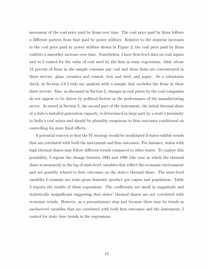
movement of the coal price paid by firms over time. The coal price paid by firms follows
a different pattern from that paid by power utilities. Relative to the stepwise increases
in the coal price paid by power utilities shown in Figure 2, the coal price paid by firms
exhibits a smoother increase over time. Nonetheless, I have firm-level data on coal inputs
and so I control for the value of coal used by the firm in some regressions. Only about
12 percent of firms in the sample consume any coal and these firms are concentrated in
three sectors: glass, ceramics and cement, iron and steel, and paper. As a robustness
check, in Section 4.8 I redo my analysis with a sample that excludes the firms in these
three sectors. Also, as discussed in Section 2, changes in coal prices by the coal companies
do not appear to be driven by political factors or the performance of the manufacturing
sector. As noted in Section 2, the second part of the instrument, the initial thermal share
of a state’s installed generation capacity, is determined in large part by a state’s proximity
to India’s coal mines and should be plausibly exogenous to firm outcomes conditional on
controlling for state fixed effects.
A potential concern is that the IV strategy would be invalidated if states exhibit trends
that are correlated with both the instrument and firm outcomes. For instance, states with
high thermal shares may follow different trends compared to other states. To explore this
possibility, I regress the change between 1994 and 1998 (the year in which the thermal
share is measured) in the log of state-level variables that reflect the economic environment
and are possibly related to firm outcomes on the state’s thermal share. The state-level
variables I examine are state gross domestic product per capita and population. Table
3 reports the results of these regressions. The coefficients are small in magnitude and
statistically insignificant suggesting that states’ thermal shares are not correlated with
economic trends. However, as a precautionary step and because there may be trends in
unobserved variables that are correlated with both firm outcomes and the instrument, I
control for state time trends in the regressions.
13
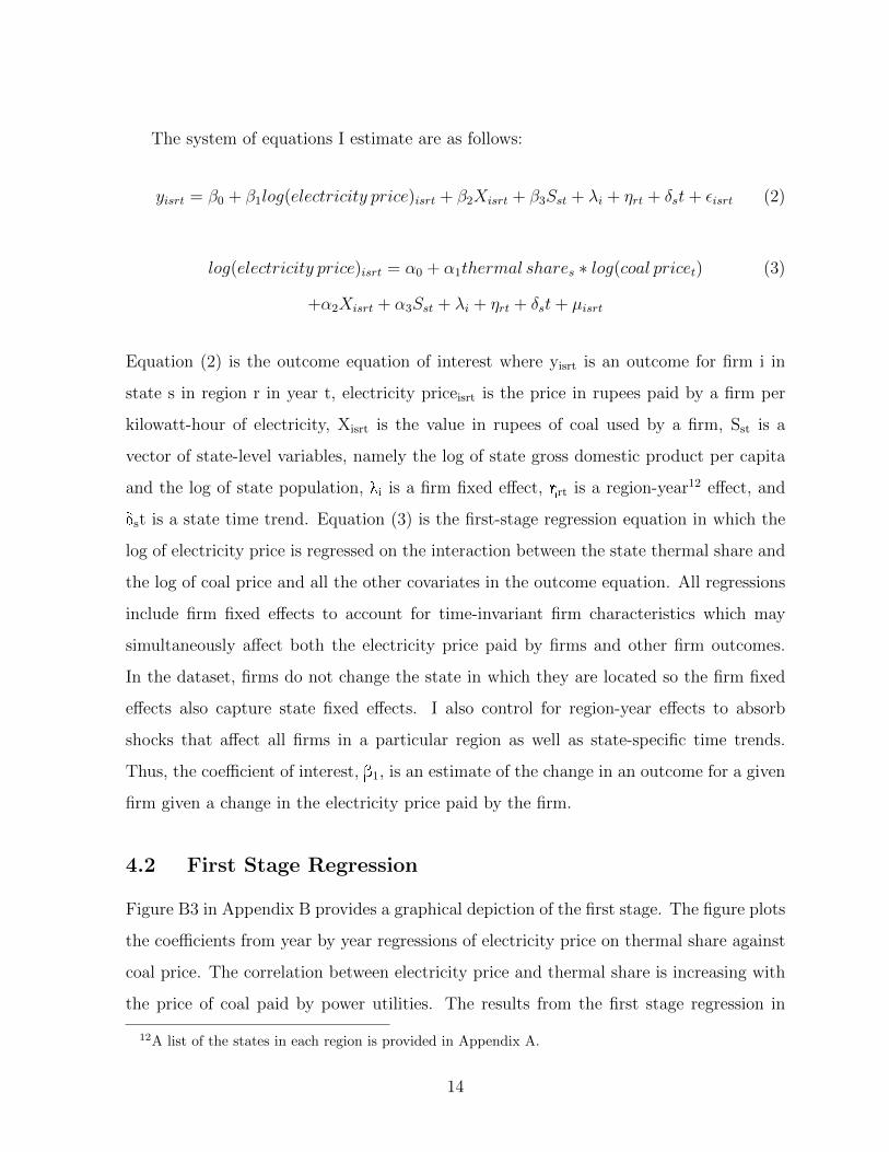
The system of equations I estimate are as follows:
yisrt = β0 + β1log(electricity price)isrt + β2Xisrt + β3Sst + λi + ηrt + δst+ εisrt (2)
log(electricity price)isrt = α0 + α1thermal shares ∗ log(coal pricet) (3)
+α2Xisrt + α3Sst + λi + ηrt + δst+ µisrt
Equation (2) is the outcome equation of interest where yisrt is an outcome for firm i in
state s in region r in year t, electricity priceisrt is the price in rupees paid by a firm per
kilowatt-hour of electricity, Xisrt is the value in rupees of coal used by a firm, Sst is a
vector of state-level variables, namely the log of state gross domestic product per capita
and the log of state population, li is a firm fixed effect, hrt is a region-year12 effect, and
dst is a state time trend. Equation (3) is the first-stage regression equation in which the
log of electricity price is regressed on the interaction between the state thermal share and
the log of coal price and all the other covariates in the outcome equation. All regressions
include firm fixed effects to account for time-invariant firm characteristics which may
simultaneously affect both the electricity price paid by firms and other firm outcomes.
In the dataset, firms do not change the state in which they are located so the firm fixed
effects also capture state fixed effects. I also control for region-year effects to absorb
shocks that affect all firms in a particular region as well as state-specific time trends.
Thus, the coefficient of interest, b1, is an estimate of the change in an outcome for a given
firm given a change in the electricity price paid by the firm.
4.2 First Stage Regression
Figure B3 in Appendix B provides a graphical depiction of the first stage. The figure plots
the coefficients from year by year regressions of electricity price on thermal share against
coal price. The correlation between electricity price and thermal share is increasing with
the price of coal paid by power utilities. The results from the first stage regression in
12A list of the states in each region is provided in Appendix A.
14

equation (3) are presented in Table 4. Since the instrument varies at the state level,
all the standard errors in the IV regressions are clustered at the state level to allow for
correlations across firms in the same state. Column 1 shows the results from the first stage
regression without controlling for state time trends. The estimate of the coefficient on
the instrument is positive and statistically different from zero at the one percent level. In
Column 2, I control for state time trends. The coefficient remains positive and statistically
significant but is smaller than the estimate in Column 1. This suggests that the coal price
trend is correlated with state-specific trends in other variables that vary with electricity
prices. I, therefore, control for state time trends in the following regressions. In Column
3, I include state-level variables, namely the log of state gross domestic product per capita
and the log of state population, as well as the value of coal consumed by the firm. The
coefficient on the instrument changes little with the inclusion of these control variables.
The results of the first-stage regressions indicate that as coal price rises, firms in states
that rely on thermal electricity generation experience an increase in electricity price. In
terms of magnitudes, the coefficient of 0.51 on the instrument in Column 3 implies that,
for instance, firms in Delhi, which has a thermal share of 57 percent, would experience a
0.3 percent increase in electricity price given a one percent increase in coal price, while
firms in West Bengal, which has a thermal share of 94 percent, would experience a 0.5
percent increase in electricity price. This magnitude is plausible given that, as noted in
Section 2, the cost of coal can account for about 66 percent of the total cost of power
production in thermal power plants (Government of India, 2006).
4.3 Effect on Electricity Consumption
Table 5 reports results on the effects of electricity prices on electricity consumption,
in kilowatt-hours, by firms. Columns 1 and 2 present estimates from OLS regressions
of equation (2). All standard errors in the OLS regressions are clustered at the firm
level to allow for correlations across years within firms. All regressions control for firm
fixed effects, state time trends and region-year effects. In addition to these controls, the
regression in Column 2 controls for the log of state gross domestic product per capita,
15

the log of state population and the value of coal consumed by the firm. The statistically
significant negative coefficients on the log of electricity price suggest that firms reduce the
quantity, in kilowatt-hours, of electricity purchased as electricity price increases. Because
of the potential endogeneity of electricity prices discussed in Section 3, caution should
be exercised in interpreting the result from the OLS regression as evidence of a causal
relationship between electricity price and firm outcomes.
Columns 3 and 4 present the reduced form results while Columns 5 and 6 present
the IV results correcting for the potential endogeneity of electricity prices. The results
from the IV regressions are similar to and permit a causal interpretation of the findings
from the OLS regression. In response to high electricity prices, firms reduce the quantity
of electricity they purchase. As indicated by the coefficients in Columns 5 and 6, a one
percent increase in electricity price leads to between a 1.19 and a 1.29 percent fall in
the quantity of electricity purchased by firms. These estimates of the price elasticity of
electricity demand are closely in line with the range (-1.25 to -1.94) found for industrial
consumers in the existing literature (Iimi, 2010).
If firms are able to generate enough electricity to offset the reduction in the quantity of
electricity purchased, then there may not be a reduction in the quantity of electricity they
use. However, as discussed in Section 3, firms primarily use self-generation to mitigate
the effects of outages rather than prices since it is much costlier for firms to generate their
own electricity than it is to purchase electricity from the power utilities. It is therefore
unlikely that firms would increase self-generation of electricity in response to an increase
in electricity price.
In Panel B of Table 5, the coefficient on the log of electricity price from regressing the
log of the total quantity of electricity used by the firm, both purchased and self-generated,
on the log of electricity price is negative and statistically significant. This result confirms
the hypothesis that firms are not able to use self-generation to offset the reduction in
the quantity of electricity purchased and therefore experience a reduction in their total
electricity consumption. To further explore the effect, if any, of electricity price on the
self-generation of electricity, Panels C and D of Table 5 report estimates from regressions
16

of an indicator variable for self-generation and the generated share of electricity on the log
of electricity price. The coefficients on the log of electricity price from the IV regressions
are negative and statistically significant implying a negative correlation between electric-
ity price and self-generation of electricity by firms. This finding is consistent with firms
switching to less electricity-intensive industries in response to an increase in electricity
price, as is shown below, and, hence, reducing their total consumption of electricity. This
reduction in total consumption would come from a reduction not only in electricity pur-
chased but also from a reduction in self-generated electricity as self-generation is costlier
than purchasing electricity from the power utilities.
4.4 Effect on Industry Choice
The reduction in the consumption of electricity as electricity price rises suggests that
firms may be altering their production to rely less on electricity in order to mitigate the
effects of high electricity prices. To become less dependent on expensive electricity, firms
may change their production to focus on goods that are less electricity-intensive. At the
5-digit level, industries within the same 4-digit industry exhibit similarities in terms of
their main inputs and final products. For instance, within the 4-digit industry code 1512
(processing and preserving of fish and fish products), the 5-digit industry code 15121 refers
to the sun-drying of fish, while code 15122 refers to the artificial dehydration of fish, which
requires the use of electrically powered drying machines. Both industries use the same
primary input, fish, and have the same end product, dried fish, but differ in terms of the
processes used, with industry 15121 using a less electricity-intensive process. Given the
similarities between 5-digit industries within the same 4-digit industry, we might expect
that firms can switch between 5-digit industries in response to changes in electricity price.
To explore this, I define the electricity intensity of a 5-digit industry as the average
kilowatt-hours of electricity consumed per rupee of output by firms in that industry.13
This corresponds to the standard measure of electricity intensity used by the International
13I define the 5-digit electricity intensities using data from 1999, which precedes the first year of thedata used in the analysis, to avoid confounding effects from endogenous changes in industries’ electricityintensities over time.
17
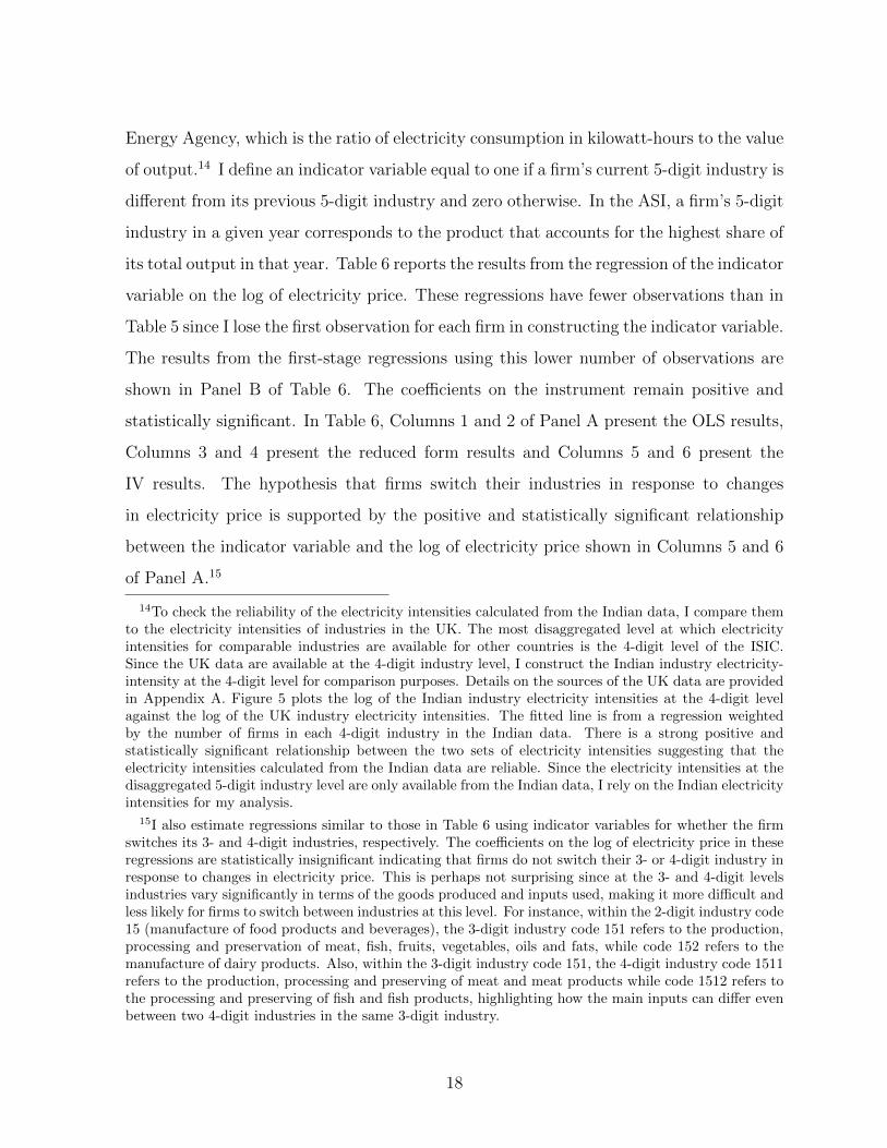
Energy Agency, which is the ratio of electricity consumption in kilowatt-hours to the value
of output.14 I define an indicator variable equal to one if a firm’s current 5-digit industry is
different from its previous 5-digit industry and zero otherwise. In the ASI, a firm’s 5-digit
industry in a given year corresponds to the product that accounts for the highest share of
its total output in that year. Table 6 reports the results from the regression of the indicator
variable on the log of electricity price. These regressions have fewer observations than in
Table 5 since I lose the first observation for each firm in constructing the indicator variable.
The results from the first-stage regressions using this lower number of observations are
shown in Panel B of Table 6. The coefficients on the instrument remain positive and
statistically significant. In Table 6, Columns 1 and 2 of Panel A present the OLS results,
Columns 3 and 4 present the reduced form results and Columns 5 and 6 present the
IV results. The hypothesis that firms switch their industries in response to changes
in electricity price is supported by the positive and statistically significant relationship
between the indicator variable and the log of electricity price shown in Columns 5 and 6
of Panel A.15
14To check the reliability of the electricity intensities calculated from the Indian data, I compare themto the electricity intensities of industries in the UK. The most disaggregated level at which electricityintensities for comparable industries are available for other countries is the 4-digit level of the ISIC.Since the UK data are available at the 4-digit industry level, I construct the Indian industry electricity-intensity at the 4-digit level for comparison purposes. Details on the sources of the UK data are providedin Appendix A. Figure 5 plots the log of the Indian industry electricity intensities at the 4-digit levelagainst the log of the UK industry electricity intensities. The fitted line is from a regression weightedby the number of firms in each 4-digit industry in the Indian data. There is a strong positive andstatistically significant relationship between the two sets of electricity intensities suggesting that theelectricity intensities calculated from the Indian data are reliable. Since the electricity intensities at thedisaggregated 5-digit industry level are only available from the Indian data, I rely on the Indian electricityintensities for my analysis.
15I also estimate regressions similar to those in Table 6 using indicator variables for whether the firmswitches its 3- and 4-digit industries, respectively. The coefficients on the log of electricity price in theseregressions are statistically insignificant indicating that firms do not switch their 3- or 4-digit industry inresponse to changes in electricity price. This is perhaps not surprising since at the 3- and 4-digit levelsindustries vary significantly in terms of the goods produced and inputs used, making it more difficult andless likely for firms to switch between industries at this level. For instance, within the 2-digit industry code15 (manufacture of food products and beverages), the 3-digit industry code 151 refers to the production,processing and preservation of meat, fish, fruits, vegetables, oils and fats, while code 152 refers to themanufacture of dairy products. Also, within the 3-digit industry code 151, the 4-digit industry code 1511refers to the production, processing and preserving of meat and meat products while code 1512 refers tothe processing and preserving of fish and fish products, highlighting how the main inputs can differ evenbetween two 4-digit industries in the same 3-digit industry.
18

To check if the industries firms switch to are less electricity-intensive, I run regres-
sions of the electricity intensity of a firm’s 5- digit industry on electricity price. Table
7 reports the estimates from these regressions. The coefficient on the log of electricity
price is negative and statistically significant supporting the idea that firms switch to less
electricity-intensive industries as electricity price rises.
Is the electricity intensity of an industry related to its productivity? This question
is an important one in understanding whether switching to less electricity-intensive in-
dustries in response to increases in electricity price has any dire consequences for firms.
If electricity-intensive industries are indeed those that rely on productivity-enhancing
technologies, then operating in a less electricity-intensive industry may affect firms’ pro-
ductivity growth. As most innovations in production processes are reliant on electricity,
we might expect it to be the case that the electricity intensity of an industry is positively
associated with both its technology intensity and productivity.
As a way of checking if a positive relationship exists between an industry’s electricity
intensity and its technology intensity, I look at the correlation between an industry’s elec-
tricity intensity and its machine intensity since, arguably, industries using more advanced
technologies are more machine-intensive. I plot the log of the electricity intensity for each
5-digit industry against the log of its machine-labor ratio in Figure 6. The fitted regression
line is weighted by the number of firms in each 5-digit industry. This plot supports the
idea that an industry’s electricity intensity is positively correlated with its machine inten-
sity, and this correlation is statistically significant. In Figure 7, I plot a similar graph to
check the correlation between an industry’s electricity intensity and its labor productivity.
Similar to the finding for machine intensity, there is a positive and statistically significant
relationship between an industry’s electricity intensity and its labor productivity.
To corroborate this finding, I examine the correlation between electricity intensity and
a variable that has been used as a proxy for product sophistication or the productivity level
of a good and has been linked to growth in the literature. This proxy is an index called
PRODY which was developed in Hausmann, Hwang, and Rodrik (2007) and has been used
in several papers including Mattoo and Subramanian (2009) and Wang, Wei, and Wong
19

(2010). PRODY is defined as the weighted average of the per capita GDPs of countries
exporting a given product, where the weights are the ratios of the share of the product
in a country’s exports to the sum of the shares for all countries exporting the product.
The motivation for this measure is the assumption that richer countries produce more
sophisticated goods. Figure 8 plots the log of electricity intensity for India against the log
of PRODY, both at the 4-digit industry level.16 The fitted line in the Figure 8 is weighted
by the number of firms in each 4-digit industry. A positive relationship is discernible
between the log of electricity intensity and the log of PRODY in the graph, lending
support to the idea that electricity-intensive industries tend to have higher productivity
levels.
4.5 Effect on Product Mix
In the previous section, I showed that firms switch to less electricity-intensive 5-digit
industries in response to an increase in electricity price. As noted above, a firm’s 5-digit
industry in a given year in the ASI corresponds to the product that accounts for the highest
share of the firm’s total output in that year. Therefore, the result that firms are switching
to a less electricity-intensive 5-digit industry indicates that firms are changing their main
product but does not provide information about the firms’ other products in the case of
multiple-product firms. About 47 percent of the firms in the dataset are multiple-product
firms and the average number of products per firm is 2.14.17 To get a sense of how a firm’s
product mix responds to changes in electricity prices, I calculate the average electricity
intensity of a firm’s product mix. I first define the electricity intensity of each product as
the average kilowatt-hours of electricity consumed per rupee of output by single-product
firms producing that product.18 A caveat here is that since single-product firms may
16I use the electricity intensity at the 4-digit instead of the 5-digit level because I am able to obtainthe PRODY values at the 4-digit industry level but not at the 5-digit industry level. Details on theconstruction of the PRODY values at the 4-digit industry level are provided in Appendix A.
17In the ASI surveys, firms are asked to list their top 10 products in terms of their contribution to thefirm’s total output. Therefore, the number of products per firm is top-coded at 10. However, almost allthe firms (98.6 percent) list fewer than 10 products. Each product is identified by a unique code fromIndia’s Annual Survey of Industries Commodity Classification (ASICC). There are 4,452 product codesin the dataset.
20
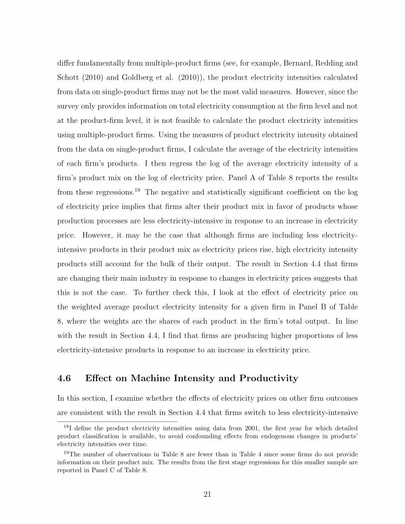
differ fundamentally from multiple-product firms (see, for example, Bernard, Redding and
Schott (2010) and Goldberg et al. (2010)), the product electricity intensities calculated
from data on single-product firms may not be the most valid measures. However, since the
survey only provides information on total electricity consumption at the firm level and not
at the product-firm level, it is not feasible to calculate the product electricity intensities
using multiple-product firms. Using the measures of product electricity intensity obtained
from the data on single-product firms, I calculate the average of the electricity intensities
of each firm’s products. I then regress the log of the average electricity intensity of a
firm’s product mix on the log of electricity price. Panel A of Table 8 reports the results
from these regressions.19 The negative and statistically significant coefficient on the log
of electricity price implies that firms alter their product mix in favor of products whose
production processes are less electricity-intensive in response to an increase in electricity
price. However, it may be the case that although firms are including less electricity-
intensive products in their product mix as electricity prices rise, high electricity intensity
products still account for the bulk of their output. The result in Section 4.4 that firms
are changing their main industry in response to changes in electricity prices suggests that
this is not the case. To further check this, I look at the effect of electricity price on
the weighted average product electricity intensity for a given firm in Panel B of Table
8, where the weights are the shares of each product in the firm’s total output. In line
with the result in Section 4.4, I find that firms are producing higher proportions of less
electricity-intensive products in response to an increase in electricity price.
4.6 Effect on Machine Intensity and Productivity
In this section, I examine whether the effects of electricity prices on other firm outcomes
are consistent with the result in Section 4.4 that firms switch to less electricity-intensive
18I define the product electricity intensities using data from 2001, the first year for which detailedproduct classification is available, to avoid confounding effects from endogenous changes in products’electricity intensities over time.
19The number of observations in Table 8 are fewer than in Table 4 since some firms do not provideinformation on their product mix. The results from the first stage regressions for this smaller sample arereported in Panel C of Table 8.
21
industries in response to high electricity prices. As shown in Section 4.4, the electricity
intensity of an industry is positively correlated with its machine intensity. Thus, if firms
are switching to less electricity-intensive industries in response to an increase in electricity
price, then we might expect their machine intensity to also fall with electricity price. The
estimates from a regression of the log of machine-labor ratio on the log of electricity price
are reported in Panel A of Table 9. The negative and statistically significant coefficients
on the log of electricity price in the IV regressions suggest that firms become less machine-
intensive as electricity prices increase in line with the finding that an industry’s electricity
intensity is positively related to its machine intensity. Next, I analyze the relationship
between labor productivity and electricity prices. Before turning to the effect of electricity
prices on firm labor productivity, I look at the effect on firm output and employment
separately. The IV results in Panels B and C of Table 9 imply that an increase in
electricity price results in a reduction in output and employment, with a much greater
reduction in output than in employment.
I present the results for the effect of electricity prices on labor productivity in Panel A
of Table 10. As implied by the results for output and labor in Table 9, labor productivity
falls with an increase in electricity price. This result is in accordance with the positive
correlation found between an industry’s electricity intensity and its labor productivity and
the previous result that firms switch to less electricity-intensive industries as electricity
prices rise. In addition to labor productivity, I also investigate the effect of electricity
prices on a firm’s total factor productivity (TFP). The results of this analysis are reported
in Panels B and C of Table 10. I construct TFP using two methods. The first measure of
TFP, which I refer to as TFP(OLS), is the residual from industry-specific OLS regressions
of the log of output on the logs of labor, capital and firm inputs. The second measure of
TFP, which I refer to as TFP (Olley-Pakes), is constructed following the method proposed
in Olley and Pakes (1996).20 Although negative, the coefficients on the log of electricity
price for the TFP regressions are not statistically significant. However, these conventional
measures of TFP may be biased since they do not take into account firm heterogeneity
20Details on the construction of the TFP measures are provided in Appendix A.
22
in input and output quality and mark-ups and so the results for the TFP measures may
not be reliable.
To summarize the results so far, an increase in electricity price causes firms to reduce
their electricity consumption and switch to less electricity-intensive industries. Consistent
with this switch and the positive correlations between an industry’s electricity intensity on
one hand and its machine intensity and productivity on the other, I find that as electricity
prices rise, firms experience a reduction in their machine intensity and labor productivity.
4.7 Effect on Firm Productivity Growth
In addition to the level effects on productivity found in the previous section, changes
in electricity prices may have growth effects on firms. In Section 4.4, I showed that
a negative relationship exists between electricity prices and the electricity intensity of
the industry in which firms choose to operate. If these electricity-intensive industries are
arguably more technologically advanced, as suggested by the positive correlations between
industry electricity intensity and machine intensity and productivity, then switching to
such industries may give firms the opportunity to use more advanced technologies. If
these technologically advanced industries generate more opportunities for learning and
further innovation than the less technologically advanced industries, then switching to
such industries may subsequently have a positive effect on firm productivity growth. To
explore this possibility, I run regressions of a firm’s productivity growth rate between
time t-1 and time t on electricity price at time t-1. I calculate the growth rate of a firm
outcome as the log difference between the firm outcome this year and the previous year.
The results from the first stage regression for the growth rate regressions are presented
in Table 11. The relationship between electricity price and the instrument remains positive
and statistically significant. Before looking at the effect of electricity price on labor
productivity growth, I present results on the effects of electricity price on the growth
rates of firm output and employment separately in Table 12. The coefficients on the log
of electricity price in the IV regressions provide some evidence that firm output growth
falls as electricity price increases. However, there is no evidence of a correlation between
23

electricity price and employment growth. The lack of an effect could be the result of two
opposing effects on employment. On one hand, firms are contracting, as suggested by the
negative effect on output, which would imply a reduction in employment growth. On the
other hand, firms are becoming more labor intensive, which would imply an increase in
employment growth. The estimates for the effect of electricity price on labor productivity
growth are reported in Table 13. The IV coefficients on the log of electricity price are
negative and statistically significant. This result is consistent with the conjecture that
an increase in electricity price, by causing firms to switch to less electricity-intensive
industries, results in fewer learning and innovation opportunities for firms and, therefore,
negatively affects their productivity growth
In addition to labor productivity growth, I also analyze the relationship between elec-
tricity price and TFP growth. The results of this analysis are presented in Panels B and
C of Table 13. Similar to the result for labor productivity, an increase in electricity price
results in a decline in the growth rate of TFP. In sum, aside from the level effects on labor
productivity and output observed in the previous section, an increase in electricity price
has persistent effects on firms by negatively affecting the growth rates of firm output,
labor productivity and TFP.
4.8 Robustness Checks
In this section, I test the robustness of my results to different specifications. In Column
2 of Table 14, I test the robustness of the results to the exclusion of the value of coal
used by the firm as a control variable. For comparison purposes, Column 1 of Table 14
presents the previous results which included this control variable. The results in Columns
1 and 2 are essentially the same implying that the results are robust to the exclusion of
the value of coal used by the firm.
A potential concern is that coal prices may be correlated directly with power outages,
independently of electricity prices, and hence the IV regressions may be picking up the
effects of power outages and not the effects of electricity prices, per se. However, as shown
in Table B3 in Appendix B, coal-related issues are not a common cause of outages in In-
24

dia. Coal-related issues accounted for between 0.8 and 4.1 percent of kilowatt-hours of
generation lost in thermal power plants due to outages over the period 2001 to 2008. I do
not have state-level data on outages. However, I have state-level data on the plant load
factor of thermal power plants.21 The plant load factor is the ratio of actual electricity
generation to the maximum possible generation of power plants and is negatively corre-
lated with outages. I therefore control for the log of the state-level plant load factor in
the regressions in Column 3 of Table 14 to proxy for the extent of outages in the state.
The results are very similar to the original results reported in Column 1. In Column 4 of
Table 14, I include both the value of coal used by the firm and the log of the state-level
plant load factor as control variables. The results are again very similar to the original
results.
An argument made in Section 4.1 to support the validity of the identification strategy
was that the coal price used in the instrument is set specifically for power utilities and
is different from the coal price paid by firms. Therefore, this coal price should not affect
firm outcomes other than through its effect on electricity price. To further alleviate any
concern that the coal price used in the instrument may affect firm outcomes directly since
some firms use coal as an input, I controlled for the value of coal used by the firm in some
regressions. As another check that my results are not being driven by a violation of the
exclusion restriction, I redo my analysis with a sample that excludes firms in sectors that
are heavily dependent on coal. The manufacturing sectors that are the largest consumers
of coal are the glass, ceramics and cement industry, the iron and steel industry, and the
paper industry.22 These three sectors have the highest proportions of coal as a share of
inputs in the dataset. Table 15 presents the main results for the sample that excludes
firms in these three sectors. Reassuringly, the conclusions from above still hold. Firms
switch to less electricity-intensive industries and experience declines in machine-intensity,
output and labor productivity as electricity prices rise.
21Details on the source of the state-level plant load factor data are provided in Appendix A.22These sectors correspond to the ISIC Rev. 3 2-digit industry codes 26, 27 and 21, respectively.
25

5 Conclusion
Drawing on Indian firm-level data, this paper analyzes the effect of electricity price on
the type of industry firms choose to operate in and the implications for their productivity
growth. Addressing the potential endogeneity of electricity prices by exploiting the nature
of electricity generation in India, I show that firms respond to increases in electricity prices
by shifting to products with less electricity-intensive production processes. I provide
evidence that an increase in electricity price has negative consequences for firm output,
labor productivity, and machine intensity. In addition to these level effects, I find that
firm output and productivity growth are negatively affected by increases in electricity
prices. Taken together, these results suggest that high electricity prices cause firms to
operate in low electricity intensity industries and hence forego the productivity-enhancing
opportunities available in more electricity-intensive and, arguably, more technologically
advanced industries.
An observed pattern in India’s manufacturing sector is that firms grow very little as
they age (Hsieh and Klenow, 2012). Explanations put forth for the poor performance
of the manufacturing sector have included, among others, the country’s restrictive labor
market regulations. The findings of this paper suggest that electricity constraints may
also contribute to the observed growth pattern. I find that high electricity prices have
negative consequences for firm output and growth and these high prices may therefore
be suppressing the expansion of India’s manufacturing sector. My analysis suggests that
even a small step towards achieving fairer pricing of electricity for industrial users could
result in significant gains in manufacturing output. As an example, industrial users were
charged about an extra 89 billion rupees to cover electricity subsidies to agricultural and
domestic users in 2008. Electricity consumption by industrial users in that year was 157
giga kilowatt-hours at a price of 4.16 rupees per kilowatt hour equivalent to total sales
of 653 billion rupees (Government of India, 2011a). Therefore, about 14 percent of the
total electricity revenue from industrial users was for the purpose of covering subsidies
to agricultural and domestic users. If these subsidies had been reduced by as little as 10
percent (that is, by 8.9 billion rupees), electricity prices for industrial users could have
26

been reduced by 1.4 percent. My results imply that a one percent fall in electricity price
leads to about a two percent 23 increase in firm output. Hence, the 1.4 percent reduction
in electricity price could have resulted in about a 2.8 percent increase in output. India’s
aggregate manufacturing output in 2008 was 7.3 trillion rupees (Government of India,
2011c). The estimated 2.8 percent increase in output would have, therefore, meant an
additional 200 billion rupees of output, which could easily have covered the 8.9 billion
rupee reduction in subsidies.
The results of this paper shed light more broadly on the literature on productivity
growth in developing countries. The findings highlight a channel through which infras-
tructure constraints may affect firm productivity. Faced with infrastructure constraints,
in this case high electricity prices, firms may use less efficient production processes in
an attempt to become less reliant on that infrastructure. Although this paper addresses
electricity specifically, one can imagine ways in which firms may change their processes in
potentially undesirable ways to cope with other infrastructure constraints.
Additionally, while most of the literature on infrastructure constraints in develop-
ing countries has focused on the availability of infrastructure, this paper emphasizes the
importance of considering the affordability of infrastructure as well. Even with the pro-
vision of infrastructure, high prices may instigate coping strategies that have negative
consequences.
A limitation of my analysis is that I do not directly observe data on the technologies
used by firms, which are generally absent from most firm-level datasets. Future data
collection efforts could elicit such information from firms. Given the important role of
technology in growth, such data would allow more in-depth analyses of the factors in-
fluencing firms’ technology choices and how these choices shape productivity growth in
developing countries.
23This estimate is from the coefficient from the IV regression of the log of output on the log of electricityprice in Table 9.
27

References
Alby, Philippe, Jean-Jacques Dethier, and Stephane Straub. 2013. “Firms Op-
erating under Electricity Constraints in Developing Countries.” World Bank Economic
Review, 27(1): 109-132.
Banerjee, Abhijit, Esther Duflo, and Nancy Qian. 2012. “On the Road: Access
to Transportation Infrastructure and Economic Growth in China.” NBER Working
Paper No. 17897.
Bernard, Andrew B., Stephen J. Redding, and Peter K. Schott. 2010. “Multiple-
Product Firms and Product Switching.” American Economic Review, 100(1): 70-97.
Bhattacharya, Saugata, and Urjit R. Patel. 2007. “The Power Sector in India: An
Inquiry into the Efficacy of the Reform Process.” India Policy Forum, 4(1): 211-283.
Borenstein, Severin. 2002. “The Trouble with Electricity Markets: Understanding
California’s Restructuring Disaster.” The Journal of Economic Perspectives, 16 (1):
191-211.
. 2005. “The Long-Run Efficiency of Real-Time Electricity Pricing.” The Energy
Journal, 26(3): 93-116.
Borenstein, Severin, James Bushnell, and Frank Wolak. 2002. “Measuring Mar-
ket Inefficiencies in California’s Restructured Wholesale Electricity Market.” American
Economic Review, 92(5): 1376-1405.
Borenstein, Severin, and Stephen Holland. 2005. “On the Efficiency of Competitive
Electricity Markets with Time-Invariant Retail Prices.” RAND Journal of Economics,
36(3): 469-493.
Davis, Steven, Cheryl Grim, and John Haltiwanger. 2008. “Productivity Disper-
sion and Input Prices: The Case of Electricity.” Center for Economic Studies Working
Paper 08-33.
Davis, Steven, Cheryl Grim, John Haltiwanger, and Mary Streitwieser. “Elec-
tricity Unit Value Prices and Purchase Quantities : U.S. Manufacturing Plants, 1963-
2000.” The Review of Economics and Statistics, forthcoming.
Department of Energy and Climate Change. 2011. “Energy Consumption in the
28

UK: Industrial Data Tables - 2011.” Department of Energy and Climate Change.
http://www.decc.gov.uk/publications/ (accessed June 11, 2012).
Dinkelman, Taryn. 2011. “The Effects of Rural Electrification on Employment: New
Evidence from South Africa.” American Economic Review, 101(7): 3078-3108.
Donaldson, Dave. 2010. “Railroads of the Raj: Estimating the Impact of Transporta-
tion Infrastructure.” NBER Working Paper No. 16487.
Duflo, Esther, and Rohini Pande. 2007. “Dams.” Quarterly Journal of Economics,
122 (2): 601-646.
Fisher-Vanden, Karen, Erin T. Mansur, and Qiong (Juliana) Wang. 2012.
“Costly Blackouts? Measuring Productivity and Environmental Effects of Electricity
Shortages.” NBER Working Paper No. 17741.
Goldberg, Pinelopi K., Amit K. Khandelwal, Nina Pavcnik, and Petia Topalova.
2010. “Multi-product Firms and Product Turnover in the Developing World: Evidence
from India.” Review of Economics and Statistics, 92(4): 1042-1049.
Government of India. 1999. Annual Report on the Working of State Electricity Boards
and Electricity Departments 1999. New Delhi: Government of India, Planning Com-
mission.
. 2002. Annual Report on the Working of State Electricity Boards and Electricity
Departments 2001-2002. New Delhi: Government of India, Planning Commission.
. 2006. “Rajya Sabha. Unstarred Question Number 1856. September 3, 2006.”
Government of India, Ministry of Power, Two Hundred and Seventh Session of the
Rajya Sabha. http://rajyasabha.nic.in/ (accessed August 12, 2012).
. 2008a. Annual Report 2007-2008. New Delhi: Government of India, Ministry of
Coal.
. 2008b. Performance Review of Thermal Power Stations 2007-08. New Delhi:
Government of India, Central Electricity Authority, Ministry of Power.
. 2008c. Provisional Coal Statistics 2007-08. New Delhi: Government of India, Coal
Controller’s Organization, Ministry of Coal.
. 2011a. Annual Report on the Working of State Power Utilities and Electricity
29
Departments 2011-2012. New Delhi: Government of India, Planning Commission.
. 2011b. National Manufacturing Policy: Press Note No. 2 (2011 Series). New
Delhi: Government of India, Ministry of Commerce and Industry.
. 2011c. “National Accounts Statistics.” Government of India, Ministry of Statistics
and Programme Implementation. http://mospi.nic.in (accessed September 28, 2012).
. 2012. Energy Statistics 2012. New Delhi: Government of India, Ministry of
Statistics and Programme Implementation.
Hausmann, Ricardo, Jason Hwang, and Dani Rodrik. 2007. “What You Export
Matters.” Journal of Economic Growth, 12(1): 1-25.
. 2006. “What You Export Matters: Dataset.”
http://www.hks.harvard.edu/fs/drodrik/research.html (accessed May 1, 2012).
Hsieh, Chang-Tai, and Peter J. Klenow. 2009. “Misallocation and Manufacturing
TFP in China and India.” Quarterly Journal of Economics, 124(4): 1403-1448.
. 2012. “The Life Cycle of Plants in India and Mexico.” NBER Working Paper No.
18133.
IEA. 2012. Energy Prices and Taxes, Quarterly Statistics, Second Quarter 2012. Paris:
IEA.
Iimi, Atsushi. 2010. “Price Elasticity of Nonresidential Demand for Energy in South
Eastern Europe.” World Bank Working Paper No. 5167.
Joskow, Paul, and Jean Tirole. 2007. “Reliability and Competitive Electricity Mar-
kets.” RAND Journal of Economics, 38(1): 60-84.
Joskow, Paul, and Catherine Wolfram. 2012. “Dynamic Pricing of Electricity.”
American Economic Review, 102(3): 381-385.
Karnataka Electricity Regulatory Commission. 2002. Tariff Order - 2002. Kar-
nataka: Karnataka Electricity Regulatory Commission.
Mattoo, Aaditya, and Arvind Subramanian. 2009. “Criss-Crossing Globaliza-
tion: Uphill Flows of Skill-Intensive Goods and Foreign Direct Investment.” Center for
Global Development Working Paper 176.
Office for National Statistics. 2010. “Annual Business Inquiry 1995-2007 - Section D:
30

Manufacturing.” Office for National Statistics. http://www.ons.gov.uk/ons/publications/re-
reference-tables.html?edition=tcm%3A77-235505 (accessed June 11, 2012).
Olley, G. Steven, and Ariel Pakes. 1996. “The Dynamics of Productivity in the
Telecommunications Equipment Industry.” Econometrica, 64(6): 1263–97.
Puller, Steven. 2007. “Pricing and Firm Conduct in California’s Deregulated Electricity
Market.” Review of Economics and Statistics, 89(1): 75-87.
Reinikka, Ritva, and Svensson, Jakob. 2002. “Coping with Poor Public Capital.”
Journal of Development Economics, 69(1): 51-69.
Restuccia, Diego, and Richard Rogerson. 2008. “Policy Distortions and Aggregate
Productivity with Heterogeneous Establishments.” Review of Economic Dynamics,
11(4): 707-720.
Rud, Juan Pablo. 2012a. “Electricity Provision and Industrial Development: Evidence
from India.” Journal of Development Economics, 97(2): 352-367.
. 2012b. “Infrastructure Regulation and Reallocations within Industry: Theory and
Evidence from Indian Firms.” Journal of Development Economics, 99(1): 116-127.
Wang, Zhi, Shang-Jin Wei, and Anna Wong. 2010. “Does a Leapfrogging Growth
Strategy Raise Growth Rate? Some International Evidence.” NBER Working Paper
No. 16390.
World Bank. 2006. “Enterprise Surveys.” World Bank. http://www.enterprisesurveys.org
(accessed July 12, 2012).
. 2012. “World Bank Group Infrastructure Commitment.” World Bank.
http://go.worldbank.org/Z2USXGBEM0 (accessed November 9, 2012).
31

Figure 1: States’ Thermal Share of Generation Capacity and Indian Coal Reserves
(87,100](79,87](54,79](37,54](6,37][0,6]
�������������� � ���������� ����� �������������
Notes: Data on installed generation capacity are from India’s Ministry of Power’s annual reports for 1997-1998 and 2002-
2003. Map of coal reserves is from MapsofIndia.com (http://www.mapsofindia.com).
32

Figure 2: Price of Coal for Power Utilities
750
800
850
900
950
pric
e of
coa
l for
pow
er u
tiliti
es (
Rs.
per
ton
ne)
2001 2002 2003 2004 2005 2006 2007 2008
Notes: Data are from the 2010-2011 issue of the Coal Directory of India published by India’s Ministry of Coal.
33
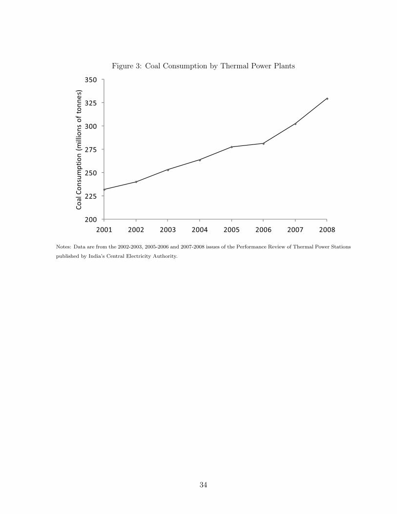
Figure 3: Coal Consumption by Thermal Power Plants
���
���
���
���
���
���
���
���� ���� ���� ���� ���� ���� ���� ���
��������������� ������������������
Notes: Data are from the 2002-2003, 2005-2006 and 2007-2008 issues of the Performance Review of Thermal Power Stations
published by India’s Central Electricity Authority.
34

Figure 4: Average Electricity Price for Different Categories of Users and Average Cost ofElectricity Supply
���
���
���
���
���
���
���
���
���
���
���
���
���
���
���
���
���
���
���
���
��� ��� ���� ��� ���� ����
������������� ����������������������
�������� ����������� ���������
�� ������ ���� ��� ���������� ��� ������ ����� ��� ��� ���������� �!���� ����"�#�$$�"
Notes: Data on electricity prices are from Government of India (1999, 2002, 2011a). Data on average cost of electricity
supply are from the Indiastat database (http://www.indiastat.com).
35

Figure 5: Indian and UK Electricity Intensities
-7-6
-5-4
-3-2
log
Indi
a el
ectr
icity
inte
nsity
-4 -3 -2 -1 0 1log UK electricity intensity
Notes: Log India electricity intensity (in rupees per kilowatt-hour) is calculated for 4-digit industries using the 1999 ASI
data. Log UK electricity intensity (in pounds sterling per kilowatt-hour) is calculated for 4-digit industries using data from
Department of Energy and Climate Change (2011) and Office for National Statistics (2010). The fitted regression line is
weighted by the number of Indian firms in each 4-digit industry. The slope of the line is 0.44 and is statistically significant
at the one percent level.
36
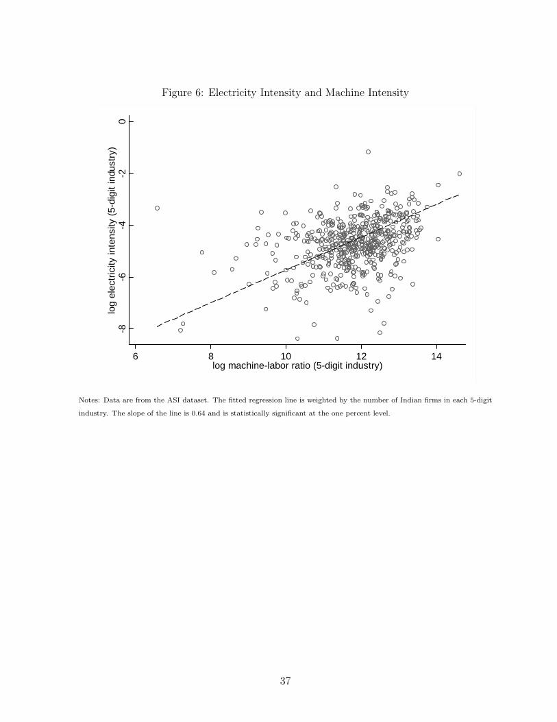
Figure 6: Electricity Intensity and Machine Intensity
-8-6
-4-2
0lo
g el
ectr
icity
inte
nsity
(5-
digi
t in
dust
ry)
6 8 10 12 14log machine-labor ratio (5-digit industry)
Notes: Data are from the ASI dataset. The fitted regression line is weighted by the number of Indian firms in each 5-digit
industry. The slope of the line is 0.64 and is statistically significant at the one percent level.
37
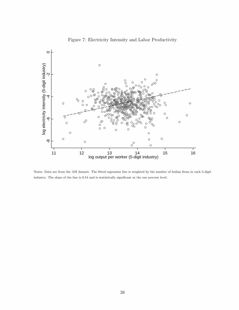
Figure 7: Electricity Intensity and Labor Productivity
-8-6
-4-2
0lo
g el
ectr
icity
inte
nsity
(5-
digi
t in
dust
ry)
11 12 13 14 15 16log output per worker (5-digit industry)
Notes: Data are from the ASI dataset. The fitted regression line is weighted by the number of Indian firms in each 5-digit
industry. The slope of the line is 0.54 and is statistically significant at the one percent level.
38
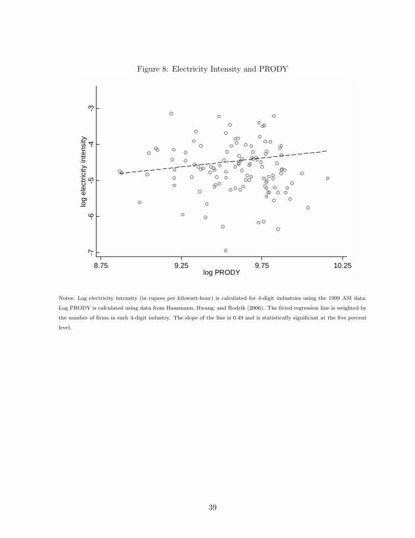
Figure 8: Electricity Intensity and PRODY
-7-6
-5-4
-3lo
g el
ectr
icity
inte
nsity
8.75 9.25 9.75 10.25log PRODY
Notes: Log electricity intensity (in rupees per kilowatt-hour) is calculated for 4-digit industries using the 1999 ASI data.
Log PRODY is calculated using data from Hausmann, Hwang, and Rodrik (2006). The fitted regression line is weighted by
the number of firms in each 4-digit industry. The slope of the line is 0.49 and is statistically significant at the five percent
level.
39
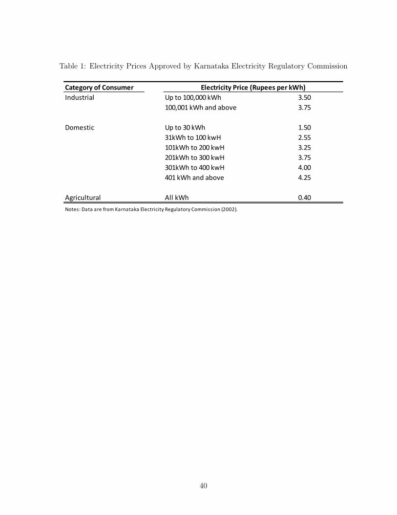
Table 1: Electricity Prices Approved by Karnataka Electricity Regulatory Commission
������������� ��� ������������������ �����������
�������� �� �� ������� ��� ����
������� ��� �� ���� ����
�������� �� �� �� ��� ����
����� �� ��� �� !���
������ �� !�� �� ��!�
!����� �� ��� �� ����
������ �� "�� �� "���
"�� ��� �� ���� "�!�
#$������� # ��� ��"�
���������������� ������������������������������������������
40

Table 2: Summary Statistics
�����������
�� ������
�������������
���� ������
����������
�� ������ ���
�������������� ���� ���� ���� ���� ����
������ ������ ������ ������
���������������� ���� ���� ���� ���� ����
������ ������ ������ ������
������������� ��!��� ���� ���� ���� ���� ����
������ ������ ������ ������
������������� ��!��� �""� ���� ���� ���� ����
������ ������ ������ ������
������������� ��!�����!�� ���� ���� ���� ����
������ ������ ������ ������
�����������#���� $��%��&��� ���� ���� ���� ����
������ ������ ������ ������
'�#� "����� ��($��� ���� ���� ����� �����
���� ���� ���� ����
)"����(*��&��� �� �� ��� ���
���� ���� ���� ����
'�#�#��*��&�� "����� ��($��#��*��&��� ���� ���� ���� ����
����� ����� ����� �����
+!��� ��� "����� ��($��� ���� ����� ����� �����
����� ����� ����� �����
+!��� �,�!����!��� "����� ��($��#��*��&��� ���� ���� ���� ����
������ ������ ������ ������
-!#��!�,�!����!��� "����� ��($��#��*��&��� ���� ���� ���� ����
������ ������ ������ ������
)���(�����.!��� � ��/��� ��/��� ��/��� ���/���
)���((��"� ��/��� �/��� ��/��� ��/���
��������������������� ���������������������������� �������������������������������
41

Table 3: Pre-Trends and Initial Thermal Share
���������������� � ������
������� �������������
���������������� � ��
������ ��������������
��� ���
���������� ������ �����
����!" �����"
#������$%��&� ��� �! �!
������������� ������������������������������������������ ����������������������������������������
����� ���������������������������������������������������������������������������������� ����� ���
�������� ����������������������������������� !������������������ ����"����������������������� ���
����������������"����#� �� �������������������$���%��&����"����'������������(���������
$�� �������������#�����������������������)*(������������������+ ���������������������������������
� ���������������#���� ������ +������������������������,�������������� ������������)*(������������
�������������#���� ������ +������������������������,�������������� ���������������+ ������---�
���������������� ������������������.� �#� ��--�������/.� �#� ������-�������� .� �#� ���0��+������������
������������������������
42

Table 4: First Stage Regression
������������� ��� ���� ��������������
��� ��� ���
����� ���� � �������� ����� �������� �������� ��������
������� ������� �������
��������� � ! �� ������� "������
�������
��������� ���#�����$� �����
�������
%��#� �& &� ���� ��$�#����$ ������
��������
'"��������� ���� (���� )$��#�$�� ���*� ����� �����
+�� �& ,-��%����$� ���.*�� ���.*�� ���.*��
+�� �& '�� ��.��� ��.��� ��.���
'� /&&���� � � �
0����$"1�� /&&���� � � �
(���� 2�� 2�$3 � �
������������� ������������������������������������������������������������ ������� ������������������
���������������� �������������������� ��� �������������� ��� ������������������ ��� ������ ���
������������������������������������ ������������������� ��� ������� ������������ ����� ��������
���� ������� �������� �����
43

Table 5: Effect of Electricity Price on Electricity Consumption
��� ��� ��������� ��������� �� ��
��� ��� ��� ��� ��� ���
���������������� ������������������������
���� ��� ������� �� ��������� ��������� ��������� ��������
������� ������� ������� �������
������� �����!��� ����� �� �������� ��������
������� �������
���������������� �����������������������������������������������
���� ��� ������� �� ��������� ��������� ��������� ���������
������� ������� ������� �������
������� �����!��� ����� �� ��������� ���������
������� �������
���������������� �������������� �
���� ��� ������� �� ���� ����� ��������� ���������
������� ������� ������� �������
������� �����!��� ����� �� ��������� ���������
������� �������
��������������� ������������������������������������
���� ��� ������� �� �������� �������� ������� ��������
������� ������� ������� �������
������� �����!��� ����� �� �������� ��������
������� �������
"��#�$% ��&���' ���(��� ���(��� ���(��� ���(��� ���(��� ���(���
"��#�)��� ��(��� ��(��� ��(��� ��(��� ��(��� ��(���
)����*##� � ! ! ! ! ! !
+���'�,����*##� � ! ! ! ! ! !
-�����.����.��'/ ! ! ! ! ! !
0'�� ! ! !
������������� ����������������������������������������������������������������������������������������� ��������� ������� ��������������� �
���������������� �����������������!"� ��� �� �������#"� ��� ������ �������!$"� ��� ���%������������������������������������������ ��������������
������ ��� ��&���������������������������'��� ��������������������������������� ��� ����� ������� ���������������������������'���������������
���'�����������(������� ������������� ��������� �������������� ������������������������������������������������� ��)��*����� ������ ����� �������
�� ��������� �������������������� ������������+,-������������������ ���������������� �����
44

Table 6: Effect of Electricity Price on Industry Switching
��� ��� ��������� ��������� �� ��
��� ��� ��� ��� ��� ���
���� ��� ������� �� ������ ������ �������� ��������
������� ������� ������� �������
������������� ��� ����� �� ������� ������������!� �������
������������� ��� ����� �� �������� ��������
������� �������
"��������� ������#�����$%���&��%�� ����� �����
'��(�)*���+���%� ���,��! ���,��! ���,��! ���,��! ���,��! ���,��!
'��(�"���� �!,��� �!,��� �!,��� �!,��� �!,��� �!,���
"����-((� ��
.���%�/����-((� ��
#�����0����0��%1
2%���
������������� ��������������������������������������������������������������������������������������� ������������������
����������� ����������!������� ������� ������!�����"��###����������������� �����������������$%� ��� ��##��������%� ��� ������#�
������$&%� ��� "��'������������������������������������������ �������������������� ��� ��(������������������������������� ������
��������������������������� ��� "���� ������� ������!���������������������������������������������������)������� ����������
��� ��������� �����"�������� ����������������������������������������������*��� �+"�,����� ������ ����� ��������� ��������� ������
�!������������ ������������-.*������������������ ���������������� ����"
���������������� ������������������������������
����������������������������� ���������������������
45

Table 7: Effect of Electricity Price on Industry Choice
������������� ��� �������������������� �������������������
��� ��� ��������� ��������� �� ��
��� ��� ��� ��� ��� ���
���� ��� ������� �� ������ ������ �������� ��������
������� ������� ������� �������
������������� ��� ����� �� ������� �������
����!�� �������
"��#�$%���&���'� ���(!�� ���(!�� ���(!�� ���(!�� ���(!�� ���(!��
"��#�)���� ��(��� ��(��� ��(��� ��(��� ��(��� ��(���
)����*##� ��
+���'�,����*##� ��
-�����.����.��'/
0'���
������������� �������������������������������������������������������������������������� ���������� ���������������������
������� ������������������ ������� ������������!��"""����������������� �����������������#$� �%� ��""��������$� �%� ������"�
������#&$� �%� !��'������������������������������������������ �������������������� �%� ��(���������������������������)��
� ��������������������������������� �%� !���� ������� ���������������������������)������������������)������������������� �
������������ ��������� �����!�������� ������������������������������������������������� ��*!�+����� �%���� ����� �������
%� ��������� �������������������� ������������,-.������������������ ���������������� ����!
46
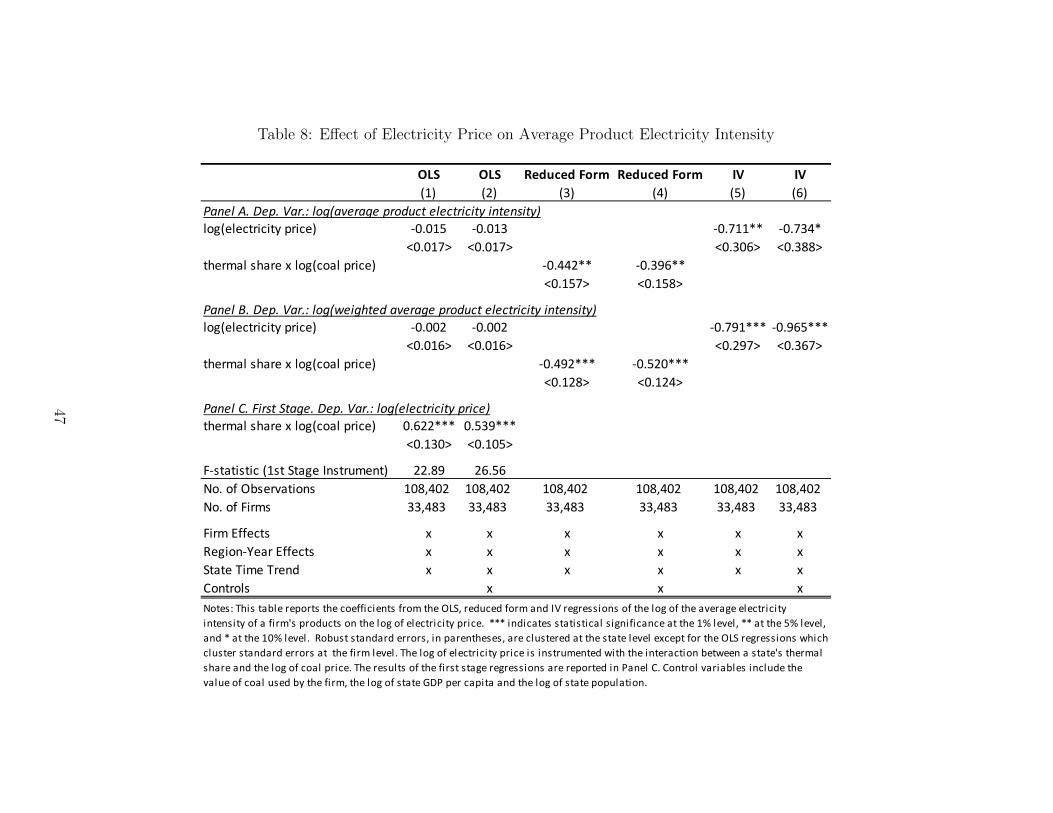
Table 8: Effect of Electricity Price on Average Product Electricity Intensity
��� ��� ��������� ��������� �� ��
��� ��� ��� ��� ��� ���
���� ��� ������� �� ������ ������ �������� �������
������� ������� ������� �������
������������� ��� ����� �� �������� ����!���
������� �������
���� ��� ������� �� ������ ������ ����!���� ���!�����
������� ������� ����!�� �������
������������� ��� ����� �� ����!���� ���������
������� �������
������������� ��� ����� �� �������� ����!���
������� �������
"��������� ������#�����$%���&��%�� ����! �����
'��(�)*���+���%� ���,��� ���,��� ���,��� ���,��� ���,��� ���,���
'��(�"���� ��,��� ��,��� ��,��� ��,��� ��,��� ��,���
"����-((� ��
.���%�/����-((� ��
#�����0����0��%1
2%���
������������� �������������������������������������������������������������������������� ������������������ ��������
���������������������������������� ������� ������������ ��!!!����������������� �����������������"#� ��� ��!!�������$#� ��� ��
����!�������"%#� ��� ��&������������������������������������������ �������������������� ��� ��'���������������������������(��
� ��������������������������������� ��� ���� ������� ���������������������������(������������������(������������������� �
������������ ��������� ����� �������� ����������������������������������������������)��� �* �*����� ������ ����� �������
�� ��������� �������������������� ������������+,)������������������ ���������������� ����
���������������� ������������������������������������������
���������������� ���������������������������������������������������
����������������������������� ����������������������47

Table 9: Effect of Electricity Price on Machine Intensity, Output and Employment
��� ��� ��������� ��������� �� ��
��� ��� ��� ��� ��� ���
���������������� �������������������������
���� ��� ������� �� ������ ����� �������� �������
������� ������� ������� �������
������������� ��� ����� �� �������� �������
�����!� �������
���������������� �����������
���� ��� ������� �� ������ ������ ���!����� ���������
������� ������� ������� �����!�
������������� ��� ����� �� ��������� ���������
������� �������
���������������� ���������������
���� ��� ������� �� ����� ����� �������� �������
������� ������� ������� �������
������������� ��� ����� �� ������ ������
������� �����!�
"��#�$%���&���'� ���(��� ���(��� ���(��� ���(��� ���(��� ���(���
"��#�)���� ��(��� ��(��� ��(��� ��(��� ��(��� ��(���
)����*##� ��
+���'�,����*##� ��
-�����.����.��'/
0'���
������������� ����������������������������������������������������������������������������������������� ��������� ������
� ��������������� ����������������� �����������������!"� ��� �� �������#"� ��� ������ �������!$"� ��� ���%���������������
��������������������������� �������������������� ��� ��&���������������������������'��� ���������������������������������
��� ����� ������� ���������������������������'������������������'�����������(������� ������������� ��������� ����������
���� ������������������������������������������������� ��)��*����� ������ ����� ��������� ��������� �������������������� ������
������+,-������������������ ���������������� �����
48
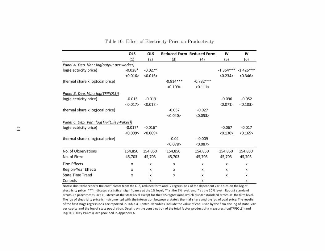
Table 10: Effect of Electricity Price on Productivity
��� ��� ��������� ��������� �� ��
��� ��� ��� ��� ��� ���
���������������� ���������������������
���� ��� ������� �� ������� ������� ��������� ���������
������� ������� ������� �������
������������� ��� ����� �� ��������� ���������
�����!� �������
���������������� ��������������
���� ��� ������� �� ������ ������ ����!� ������
������� ������� ������� �������
������������� ��� ����� �� ������ ������
������� �������
���������������� ����������������������
���� ��� ������� �� ������� ������� ������ ������
�����!� �����!� ������� �������
������������� ��� ����� �� ����� �����!
������� �������
"��#�$%���&���'� ���(��� ���(��� ���(��� ���(��� ���(��� ���(���
"��#�)���� ��(��� ��(��� ��(��� ��(��� ��(��� ��(���
)����*##� ��
+���'�,����*##� ��
-�����.����.��'/
0'���
������������� ����������������������������������������������������������������������������������������� ��������� ������
� ��������������� ����������������� �����������������!"� ��� �� �������#"� ��� ������ �������!$"� ��� ���%���������������
��������������������������� �������������������� ��� ��&���������������������������'��� ��������������������������������� ��� ��
��� ������� ���������������������������'������������������'�����������(������� ������������� ��������� �������������� ���
���������������������������������������������� ��)��*����� ������ ����� ��������� ��������� �������������������� ������������+,-�
����������������� ���������������� ������,��� ������������������������������ ����������������������������� ��.�/-.���00�����
��.�/-.� ��1-�2��00����������������3�����&�3�
49
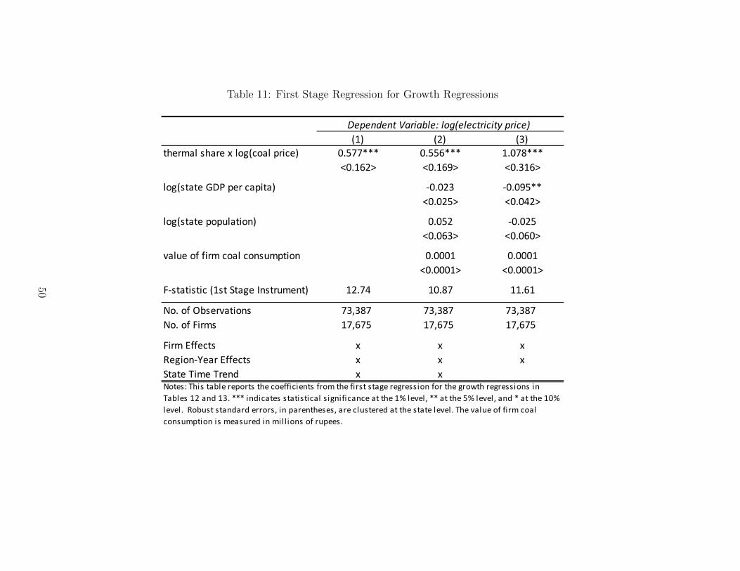
Table 11: First Stage Regression for Growth Regressions
������������� ��� ���� ��������������
��� ��� ���
����� ���� � �������� ����� �������� �������� ��������
������� ������� �������
��������� � ! �� ������� "����� "�������
������� ����#��
��������� ���$�����%� ����� "�����
������� �������
&��$� �' '� ���� ��%�$����% ������ ������
�������� ��������
("��������� ���� )���� *%��$�%�� ����# ����� �����
+�� �' ,-��&����%� ��.��� ��.��� ��.���
+�� �' (�� ��.��� ��.��� ��.���
(� /''���� � � �
0����%"1�� /''���� � � �
)���� 2�� 2�%3 � �������������� �������������������������������������������������������������������������������
��� ���������������������������������� �������������������� ��� �������������� ��� ��������������� ��
��� ���!��"��������������������������������������� "������������������� ��� ������� "������������ �
����"������������"������� ��������"�����
50
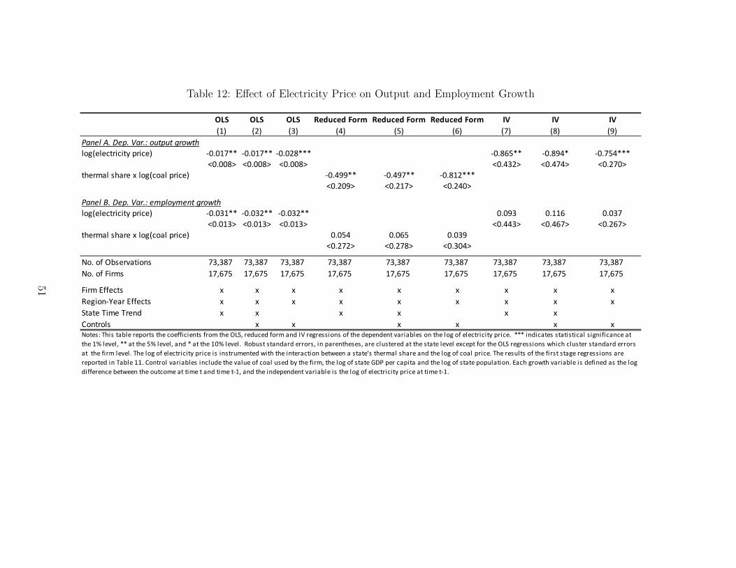
Table 12: Effect of Electricity Price on Output and Employment Growth
��� ��� ��� ��������� ��������� ��������� �� �� ��
��� ��� ��� ��� ��� ��� �� �� ���
���������������� �������������
� �������������������� ������� ������� �������� ������� ������ ��������
������ ������ ������ ������� ������ ������
�������� �����!�� ��� ��������� �������� ������� ��������
������� ������ �������
���������������� �����������������
� �������������������� �������� �������� �������� ����� ����� ����
������� ������� ������� ������� ������ ������
�������� �����!�� ��� ��������� ����� ����� �����
������ ����� �������
" �� #�$% ��&��� ' �(� �(� �(� �(� �(� �(� �(� �(� �(�
" �� #�)��� �(�� �(�� �(�� �(�� �(�� �(�� �(�� �(�� �(��
)����*##��� ! ! ! ! ! ! ! ! !
+��� '�,����*##��� ! ! ! ! ! ! ! ! !
-�����.����.��'/ ! ! ! ! ! !
0 '�� � ! ! ! ! ! !
������������� ����������������������������������������������������������������������������������������� ��������� ������� ��������������� ����������������� ��������������
���!"� ��� �� �������#"� ��� ������ �������!$"� ��� ���%������������������������������������������ �������������������� ��� ��&���������������������������'��� ����������������������
����������� ��� ����� ������� ���������������������������'������������������'�����������(������� ������������� ��������� �������������� �����������������������������������
�������������� ��!!��)����� ������ ����� ��������� ��������� �������������������� ������������*+,������������������ ���������������� ������-������'������� ����������������� ���
�������������'���������������������������������.!������������������������� ������� ������� ���������������������.!�
51
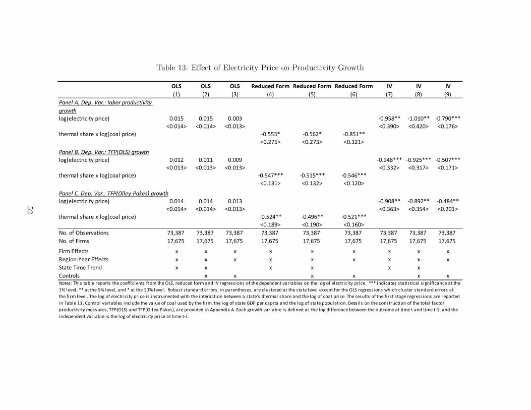
Table 13: Effect of Electricity Price on Productivity Growth
��� ��� ��� ��������� ��������� ��������� �� �� ��
��� ��� ��� ��� ��� ��� �� �� ���
���������������� �������������������
������
� �������������������� ����� ����� ����� ������� �������� ��������
������� ������� ������� ������� ������� ������
�������� �����!�� ��� ��������� ������� ������� �������
������ ������ �������
���������������� ������� !�������
� �������������������� ����� ����� ����� �������� ��������� ��������
������� ������� ������� ������� ������ ������
�������� �����!�� ��� ��������� �������� ��������� ���������
������� ������� �������
������"��������� ����������#��$�%!�������
� �������������������� ����� ����� ����� ������� ������� �������
������� ������� ������� ������� ������� �������
�������� �����!�� ��� ��������� �������� �������� ���������
������ ������� �������
" �� #�$% ��&��� ' �(� �(� �(� �(� �(� �(� �(� �(� �(�
" �� #�)��� �(�� �(�� �(�� �(�� �(�� �(�� �(�� �(�� �(��
)����*##��� ! ! ! ! ! ! ! ! !
+��� '�,����*##��� ! ! ! ! ! ! ! ! !
-�����.����.��'/ ! ! ! ! ! !
0 '�� � ! ! ! ! ! !
������������� ����������������������������������������������������������������������������������������� ��������� ������� ��������������� ����������������� �����������������
!"� ��� �� �������#"� ��� ������ �������!$"� ��� ���%������������������������������������������ �������������������� ��� ��&���������������������������'��� ��������������������������
������� ��� ����� ������� ���������������������������'������������������'�����������(������� ������������� ��������� �������������� ��������������������������������������������
����� ��!!��)����� ������ ����� ��������� ��������� �������������������� ������������*+,������������������ ���������������� ������+��� ������������������������������ ��������
����������������������-,.���/������-,.� ��0,�1��/����������������2�����&�2��3������'������� ����������������� ����������������'���������������������������������0!���������
���������������� ������� ������� ���������������������0!�
52
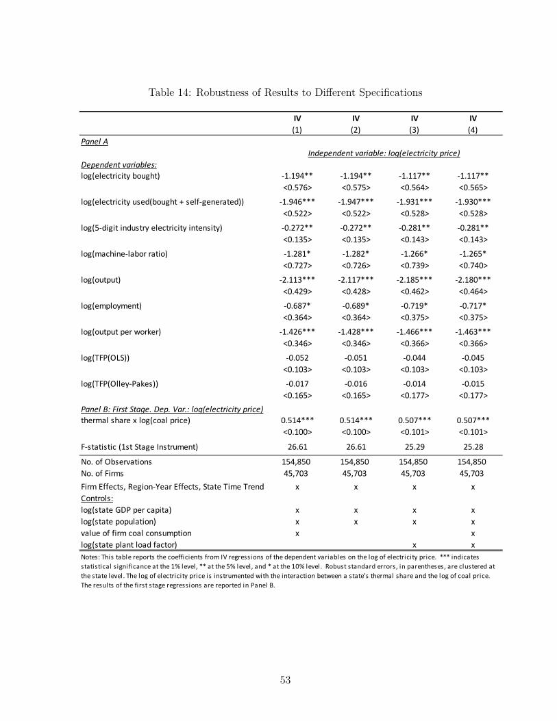
Table 14: Robustness of Results to Different Specifications
�� �� �� ��
��� ��� ��� ���
�������
����������� ���������������� ������ ����
���������� �������
������ ������������ �������� �������� �������� ��������
������� ������� ������� �������
������ ���������������� ���!�" #���� ��������� ��������� ��������� ���������
������� ������� �����$� �����$�
�����������"���� ����� �������"�"����� �������� �������� ����$��� ����$���
������� ������� ������� �������
���%#���"��#�� � #���� ����$�� ����$�� ������� �������
������� ������� ������� �������
������&��� ��������� ��������� ����$���� ����$����
������� �����$� ������� �������
���%&���%"�� ����$�� ����$�� ������� �������
������� ������� ������� �������
������&���& �'� ( � ��������� �����$��� ��������� ���������
������� ������� ������� �������
���)*+�,-.�� ������ ������ ������ ������
������� ������� ������� �������
���)*+�,����+#(��� ������ ������ ������ ������
������� ������� ������� �������
����������� ���������������� ������������ ������ ����
�� %#����# �/������#��& ��� �������� �������� �������� ��������
������� ������� ������� �������
*���#������������.�#�0"�� �%"�� ����� ����� ����� ����$
1����!�,�� 2#���"� ���3$�� ���3$�� ���3$�� ���3$��
1����!�*� %� ��3��� ��3��� ��3��� ��3���
*� %�4!!���3�5��"�6# �4!!���3�.�#��)�%�) "� / / / /
7�"� ���8
�����#��9:+�& ��#&��#� / / / /
�����#��&�&��#���"� / / / /
2#����!�!� %���#����"��%&���" / /
�����#��&�#"����#��!#��� � / /
������������� ���������������������������������������������������������������� ��������� ������� ���������������������������
�������� �������������������� ��� �������������� ��� ��������������� �� ��� ���!��"��������������������������������������� "����������
��������� ��� ����� ������� �������������������"�������#������������������#�����������$������� ������������� ��������� �������
������" ����������������������������������������������%��� �&�
53

Table 15: Effect of Electricity Price for Sample Excluding Coal-Reliant Sectors
�� ��
��� ���
�������
����������� ���������������� ������ ����
���������� �������
���������� ������� ��������� ���������
������� �������
���������� ������������ ����!���"��#���� ����$$��� �����$���
������� �������
������������"���� ������� ��"�"�� � ���$���� ����$��
������� ����$$�
����%#��"���#�����#��� �������� �������
������� �����$�
������&�� �����$��� ���$�����
���$��� �������
�����%&�� %�"� ������ ������
������� ���$���
������&��&���'��(��� ��������� ���������
����$�� ���$�$�
����)*+�,-.�� �������� ��������
������� �������
����)*+�,��� �+#(���� ������ ������
������� �������
����������� ���������������� ������������ ������ ����
���%#����#���/������#��&���� �������� ��������
������� �������
*��#��������.#���0"���%�"� $���� �����
1����!�,����2#��"� ���3��� ���3���
1����!�*��%� $�3��� $�3���
*��%�4!!�� / /
5����"�6�#��4!!�� / /
.#��)�%��)��"� / /
7�"���� /
������������� ���������������������������������������������������������������� ��������� ������� ��������
�������������� ����� ��������������� ��� ����������������� ������ ����������������������������������������
�������� ���������������������������������������������������� ����������������� !� ��� �����������"!� ��� ��
������������ #!� ��� ���$������������������������������������������ �������������������� ��� ����� ������
� ���������������������������%������������������%�����������&������� ������������� ��������� ����������
���� ����������������������������������������������'��� �(��)����� ������ ����� ��������� ��������� ���������
����������� ������������*+'������������������ ���������������� �����
54

A Appendix: Data
A.1 States Classified as Industrially Backward in the ASI
The population of factories covered by the ASI is divided into two categories: a census
sector and a sample sector. The census sector consists of all large factories and all facto-
ries in states classified as industrially backward by the government. All the factories in
the census sector are surveyed each year. A third of the remaining factories which make
up the sample sector are randomly selected each year for the survey. For the 2001 to 2005
surveys, large factories were defined as those with 200 or more workers. From the 2006
survey onwards, the definition was changed to those with 100 or more workers. For the
2001 to 2004 surveys, twelve states were classified as industrially backward. These states
are Himachal Pradesh, Jammu and Kashmir, Manipur, Meghalaya, Nagaland, Tripura,
Puducherry, Andaman and Nicobar Islands, Chandigarh, Goa, Daman and Diu, Dadra
and Nagar Haveli. From the 2005 survey onwards, only 5 states were classified as industri-
ally backward. These states are Manipur, Meghalaya, Nagaland, Tripura, and Andaman
and Nicobar Islands.
A.2 State-Level Variables
The state-level variables used in my analysis are the state gross domestic product, state
population and the plant load factor of thermal power plants in the state. The gross
domestic product and population data are from the Central Statistics Office, National
Account section of the Ministry of Statistics and Programme Implementation’s website
(http://mospi.nic.in). The data on the plant load factor of thermal power plants are
from the the 2001-2002 issue of the Annual Report on the Working of State Electricity
Boards and Electricity Departments and the 2011-2012 issue of the Annual Report on
the Working of State Power Utilities and Electricity Departments published by India’s
Planning Commission, and the Indiastat database (http://www.indiastat.com).
55
A.3 Regions
The country is divided into the following regions which are used for the region-year effects
in the regressions: Northern comprising the states of Haryana, Himachal Pradesh, Jammu
and Kashmir, Punjab, Rajasthan, Delhi and Chandigarh, Central comprising the states of
Chhattisgarh, Uttarakhand, Uttar Pradesh and Madhya Pradesh, Eastern comprising the
states of Bihar, Jharkhand, Orissa, and West Bengal, Western comprising the states of
Goa, Gujarat, Maharashtra, Daman and Diu, and Dadra and Nagar Haveli, Southern com-
prising the states of Andhra Pradesh, Karnataka, Kerala, Tamil Nadu and Puducherry,
and Northeastern comprising the states of Assam, Arunachal Pradesh, Manipur, Tripura,
Mizoram, Meghalaya and Nagaland.
A.4 UK Electricity Intensity
The electricity intensities of the UK industries are calculated using data on industry-
level electricity consumption from the UK Department of Energy and Climate Change
(Department of Energy and Climate Change, 2011) and data on industry-level output
from the UK Annual Business Inquiry (Office for National Statistics, 2010). The UK
data are available at the 4-digit level of the SIC 2003 which is identical to the 4-digit level
of the NACE Rev 1.1. I converted the SIC 2003 codes to the ISIC Rev. 3 codes (which
are identical to India’s NIC 1998 codes at the 4-digit level) using a concordance between
the NACE Rev 1.1 and the ISIC Rev. 3 codes from the website of the United Nations
Statistics Division (http://unstats.un.org).
A.5 Industry-Level PRODY
The PRODY data are obtained from Hausmann, Hwang, and Rodrik (2006). The data
are available for products at the 6-digit level of the Harmonized System (HS). Using a
concordance between the HS codes and the ISIC Rev. 3 4-digit industry codes from the
World Bank’s World Integrated Trade Solution (WITS) system, I calculate the PRODY
for each 4-digit industry as the average of the PRODY values for the HS products within
56
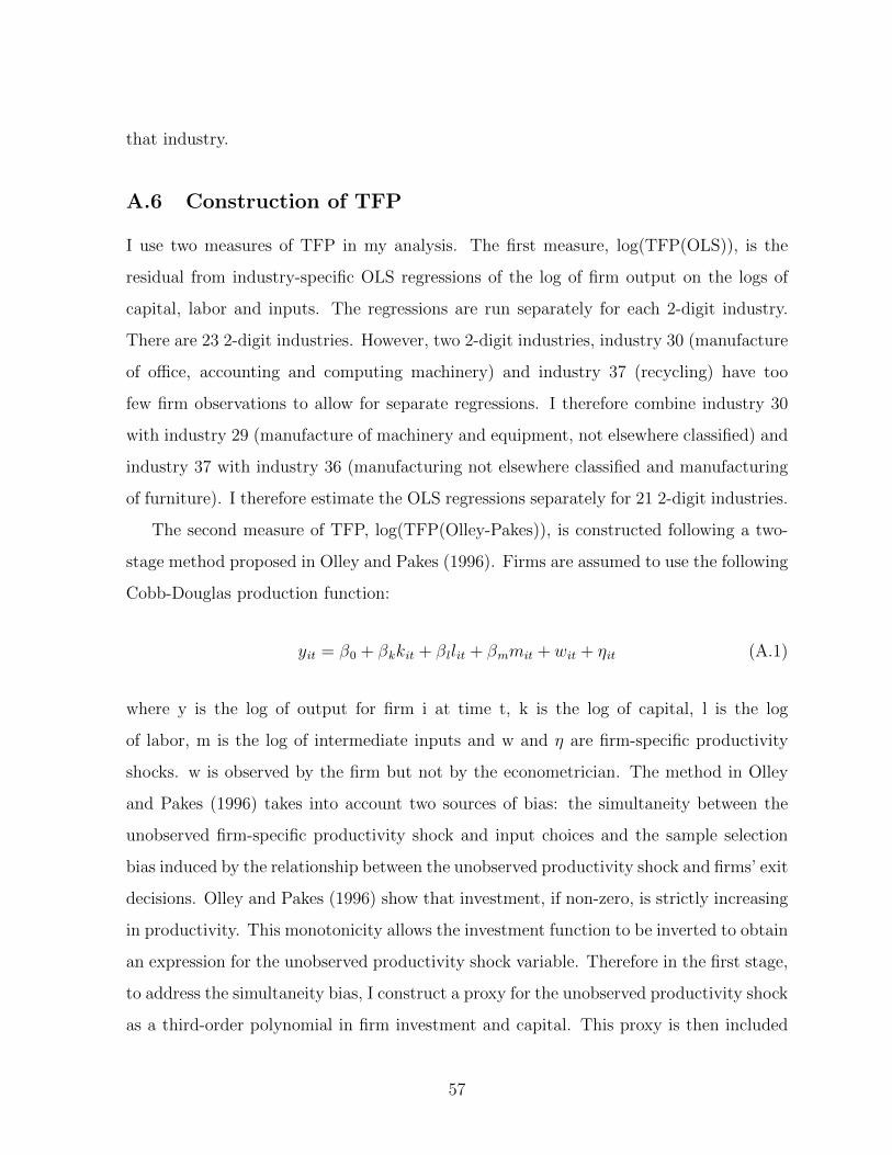
that industry.
A.6 Construction of TFP
I use two measures of TFP in my analysis. The first measure, log(TFP(OLS)), is the
residual from industry-specific OLS regressions of the log of firm output on the logs of
capital, labor and inputs. The regressions are run separately for each 2-digit industry.
There are 23 2-digit industries. However, two 2-digit industries, industry 30 (manufacture
of office, accounting and computing machinery) and industry 37 (recycling) have too
few firm observations to allow for separate regressions. I therefore combine industry 30
with industry 29 (manufacture of machinery and equipment, not elsewhere classified) and
industry 37 with industry 36 (manufacturing not elsewhere classified and manufacturing
of furniture). I therefore estimate the OLS regressions separately for 21 2-digit industries.
The second measure of TFP, log(TFP(Olley-Pakes)), is constructed following a two-
stage method proposed in Olley and Pakes (1996). Firms are assumed to use the following
Cobb-Douglas production function:
yit = β0 + βkkit + βllit + βmmit + wit + ηit (A.1)
where y is the log of output for firm i at time t, k is the log of capital, l is the log
of labor, m is the log of intermediate inputs and w and η are firm-specific productivity
shocks. w is observed by the firm but not by the econometrician. The method in Olley
and Pakes (1996) takes into account two sources of bias: the simultaneity between the
unobserved firm-specific productivity shock and input choices and the sample selection
bias induced by the relationship between the unobserved productivity shock and firms’ exit
decisions. Olley and Pakes (1996) show that investment, if non-zero, is strictly increasing
in productivity. This monotonicity allows the investment function to be inverted to obtain
an expression for the unobserved productivity shock variable. Therefore in the first stage,
to address the simultaneity bias, I construct a proxy for the unobserved productivity shock
as a third-order polynomial in firm investment and capital. This proxy is then included
57
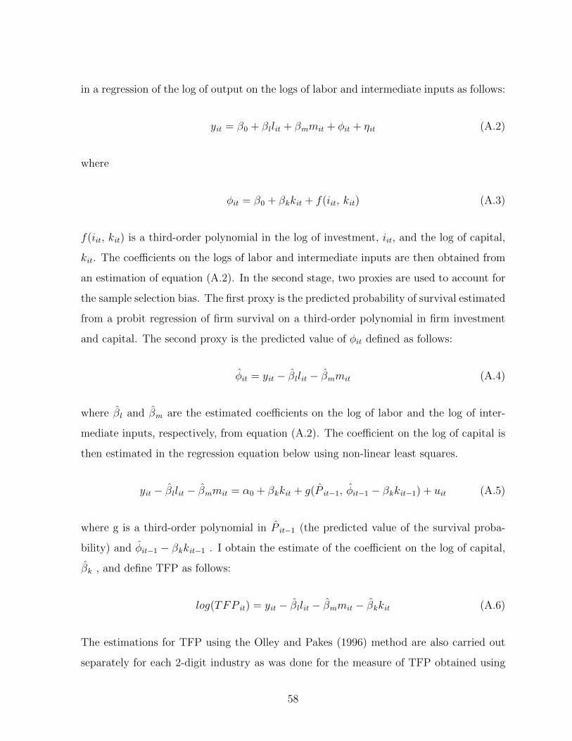
in a regression of the log of output on the logs of labor and intermediate inputs as follows:
yit = β0 + βllit + βmmit + φit + ηit (A.2)
where
φit = β0 + βkkit + f(iit, kit) (A.3)
f(iit, kit) is a third-order polynomial in the log of investment, iit, and the log of capital,
kit. The coefficients on the logs of labor and intermediate inputs are then obtained from
an estimation of equation (A.2). In the second stage, two proxies are used to account for
the sample selection bias. The first proxy is the predicted probability of survival estimated
from a probit regression of firm survival on a third-order polynomial in firm investment
and capital. The second proxy is the predicted value of φit defined as follows:
φ̂it = yit − β̂llit − β̂mmit (A.4)
where β̂l and β̂m are the estimated coefficients on the log of labor and the log of inter-
mediate inputs, respectively, from equation (A.2). The coefficient on the log of capital is
then estimated in the regression equation below using non-linear least squares.
yit − β̂llit − β̂mmit = α0 + βkkit + g(P̂ it−1, φ̂it−1 − βkkit−1) + uit (A.5)
where g is a third-order polynomial in P̂ it−1 (the predicted value of the survival proba-
bility) and φ̂it−1 − βkkit−1 . I obtain the estimate of the coefficient on the log of capital,
β̂k , and define TFP as follows:
log(TFP it) = yit − β̂llit − β̂mmit − β̂kkit (A.6)
The estimations for TFP using the Olley and Pakes (1996) method are also carried out
separately for each 2-digit industry as was done for the measure of TFP obtained using
58

OLS regressions described above.
59

B Appendix: Figures and Tables
Figure B.1: States’ Thermal Share of Generation Capacity
050
100
050
100
050
100
050
100
050
100
1998 2003 2007 1998 2003 2007 1998 2003 2007 1998 2003 2007
1998 2003 2007 1998 2003 2007 1998 2003 2007 1998 2003 2007
1998 2003 2007 1998 2003 2007 1998 2003 2007 1998 2003 2007
1998 2003 2007 1998 2003 2007 1998 2003 2007 1998 2003 2007
1998 2003 2007
ANDHRA PRADESH ASSAM BIHAR CHHATTISGARH
DELHI GUJARAT HARYANA JHARKHAND
KARNATAKA MADHYA PRADESH MAHARASHTRA ORISSA
PUNJAB RAJASTHAN TAMIL NADU UTTAR PRADESH
WEST BENGAL
ther
mal
sha
re o
f gen
erat
ion
capa
city
(%
)
Notes: Data on installed generation capacity are from India’s Ministry of Power’s annual reports for 1997-1998, 2002-2003 and 2006-2007. For Jharkhand and Chhattisgarh,
the earliest year for which data on installed generation capacity is available is 2003 since these states were created in late 2000.
60

Figure B.2: Price of Coal for Firms
2000
2500
3000
3500
pric
e of
coa
l for
firm
s (R
s. p
er to
nne)
2001 2002 2003 2004 2005 2006 2007 2008
Notes: Data are from the ASI dataset.
61

Figure B.3: Electricity Price-Thermal Share Correlations vs. Coal Price
Notes: This figure plots the coefficients from year by year regressions of the log of electricity price on thermal share against
the log of the price of coal paid by power utilities. The dashed line is a fitted regression line.
62
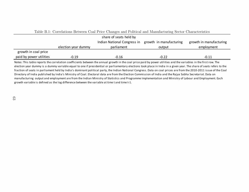
Table B.1: Correlations Between Coal Price Changes and Political and Manufacturing Sector Characteristics
������������� ��
��������������������
�������������������������
��������
������������� ��� ����
� �� �
������������ ��� �����
���������
��������������������
������������ �������� ����� ����� ����� �����
������������� ������������������ �������������������������������� ��������������� ��������������������� ���������������� ���������������������
� �������������������������������� ������ ������������������� ������� ���������� ������������� ��������������������������������������������������������
���������������������� ������� ���������������������� ��� ����������������������� � ���������!���������� �������������������"#$#%"#$$������������ �� �
!������������������� ��������������&��������� �� ��' ������ ������������������' ������ �����������������������(�)���*����*�����������!�������
���������������������������� �������������������������&���������*������������+������������ ��������������&���������,����������'�� ��������'���
����������� ����������������� ����������������������������� ��������������������%$�
63
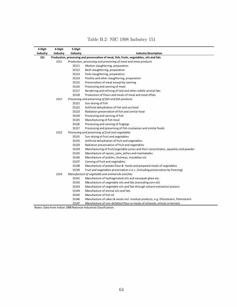
Table B.2: NIC 1998 Industry 151
��������
���� �
��������
���� �
��������
���� � ���� ������ �����
���
����
����� ���������� �������������������
����� �������� �������������������
����� �������� �������������������
����� ������������� ������ �������������������
����� ���������������������� ����!�� ������
����" ��� ��������� ��������������
����# $����������������������������������� ������!�����������
����% ����� ������������������������������������������
����
����� &���������������
����� '����� ����� �������������� ������������
����� $�������������������������� ���������������
����� ��� ��������� ������������
����� ������ ������������ ����
����" ��� ��������� ����������������
����# ��� ������������������������ � ���� ������������������
����
����� &�����������������������������!�
����� '����� ����� ����������������������������!�
����� $����������������������������������������!�
����� ������ ���������������(������!��)�� ������� ���� �� ���������*�� ��������+���
����� ������ ���������� ���)����)����������������
����" ������ ���������� ���� �����������!!���� ,
����# -��������������������������!�
����%
����.
����
�����
�����
�����
�����
����� ������ ���������� ���
����" ������ �������� ����/������� ,������������� ����,�,�0�������������������
����# ������ ���������������������������������������������������������
1���2�3���������4�������..%�1�������4��������-���� �����,
������ ������������������������
������ ��������������������/��������������������������������!�
5���������������!���������������,�, ,�6�� ������������������!������7���8
������ �������� ����������������������������� ����� ,
������ ��������������!�������������6�� ������ ������8
������ ��������������!�������������� ���� ������������ �������� �
� ��������� ����������� ��� ���������������������� �����������������������������
����� ����������� ������������� �������������������������
������� ������������� ������� ������� ���������
������� ������������� �������� ���������������
���������������������������� ����� ����������
64

Table B.3: Causes of Outages in Thermal Power Plants in India
������������� �� ������������������������� ��������� ��������
���� ���� ���� ���� ���� ���� ��� ���!
"����#$��%&�� ��'� ��'! � '� ��'� ��'� � ' �('� ��'�
)�*���� +�#$��%&�� �'� �'� �'� �'� �' �'� �'� �'�
,��� -��./�0��� �'� �'� �'! �'� �'� �'� �' �'!
/� �1� ��0������ ��'� '( ��'( ��'� ��' ��'( ��'� ��'�
���/��/������������2
./� ����������� �'� �'� �'� �'� �'� �'� �'� �'�
�����1��0����3����� �'� �'� �'� �'� �'� �'� �'� �'�
4������ �'� �'� �'� �'� �'� �'� �'� �'�
��� �5����+����� �'� �'� �'� �'� �'� �'� �'� �'�
"������������������3����� �'� �'� �'� �'� �'� �'� �'� �'�
����������3����� �'( �'� �'! �'� �'� �'� �'( �'�
������0�"��������� �('� � '� ��' � '� ��'� ��'� ��'( �!'�
���� ��� ��� ��� ��� ��� ��� ��� ���
�������������� ����������������� ��������������������������������������������������������������������������� ������
����� �������!����� ���� ������"�# ���$��%� ��� �& ��������"�'������"(
65