Electricity and Magnetism Electric Fieldsnebula2.deanza.edu/~lanasheridan/4B/Phys4B-Lecture5.pdf ·...
29
Electricity and Magnetism Electric Fields Lana Sheridan De Anza College Jan 12, 2018
Transcript of Electricity and Magnetism Electric Fieldsnebula2.deanza.edu/~lanasheridan/4B/Phys4B-Lecture5.pdf ·...
Electricity and MagnetismElectric Fields
Lana Sheridan
De Anza College
Jan 12, 2018
Last time
• Forces at a fundamental level
• Electric field
• net electric field
• electric field lines
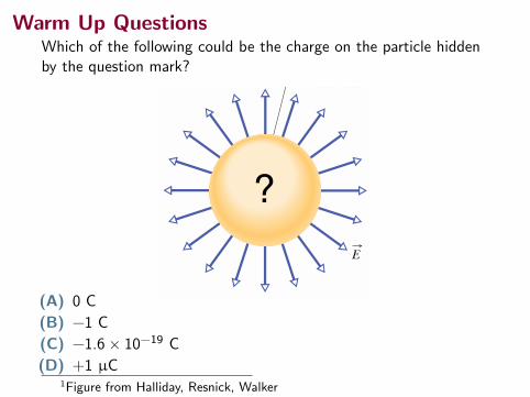
Warm Up QuestionsWhich of the following could be the charge on the particle hiddenby the question mark?
HALLIDAY REVISED
23-1 One of the primary goals of physics is to find simple ways of solvingseemingly complex problems. One of the main tools of physics in attaining thisgoal is the use of symmetry. For example, in finding the electric field of thecharged ring of Fig. 22-10 and the charged rod of Fig. 22-11, we considered thefields of charge elements in the ring and rod. Then we simplifiedthe calculation of by using symmetry to discard the perpendicular componentsof the vectors.That saved us some work.
For certain charge distributions involving symmetry, we can save far more workby using a law called Gauss’ law, developed by German mathematician and physi-cist Carl Friedrich Gauss (1777–1855). Instead of considering the fields ofcharge elements in a given charge distribution, Gauss’ law considers a hypothetical(imaginary) closed surface enclosing the charge distribution.This Gaussian surface,as it is called, can have any shape, but the shape that minimizes our calculations ofthe electric field is one that mimics the symmetry of the charge distribution. For ex-ample, if the charge is spread uniformly over a sphere, we enclose the sphere with aspherical Gaussian surface, such as the one in Fig. 23-1, and then, as we discuss inthis chapter, find the electric field on the surface by using the fact that
dE:
dE:
E:
(!k dq/r 2)dE:
E:
G A U S S ’ L A W 23C H A P T E R
605
W H AT I S P H YS I C S ?
Gauss’ law relates the electric fields at points on a (closed) Gaussian surface to thenet charge enclosed by that surface.
We can also use Gauss’ law in reverse: If we know the electric field on a Gaussiansurface, we can find the net charge enclosed by the surface. As a limited example,suppose that the electric field vectors in Fig. 23-1 all point radially outward from thecenter of the sphere and have equal magnitude. Gauss’ law immediately tells us thatthe spherical surface must enclose a net positive charge that is either a particle ordistributed spherically. However, to calculate how much charge is enclosed, we needa way of calculating how much electric field is intercepted by the Gaussian surface inFig. 23-1.This measure of intercepted field is called flux, which we discuss next.
23-2 FluxSuppose that, as in Fig. 23-2a, you aim a wide airstream of uniform velocity ata small square loop of area A. Let " represent the volume flow rate (volume per unittime) at which air flows through the loop.This rate depends on the angle between and the plane of the loop. If is perpendicular to the plane, the rate " is equal to vA.
If is parallel to the plane of the loop, no air moves through the loop, so" is zero. For an intermediate angle u, the rate " depends on the component of
normal to the plane (Fig.23-2b).Since that component is v cos u, the rate of volumeflow through the loop is
" ! (v cos u)A. (23-1)
This rate of flow through an area is an example of a flux—a volume flux in thissituation.
v:
v:v:
v:
v:
Fig. 23-1 A spherical Gaussian surface. If the electric field vectorsare of uniform magnitude and pointradially outward at all surface points,you can conclude that a net positivedistribution of charge must lie withinthe surface and have spherical symmetry.
SphericalGaussiansurface
?E
halliday_c23_605-627v2.qxd 18-11-2009 15:34 Page 605
(A) 0 C
(B) −1 C
(C) −1.6× 10⁻¹⁹ C
(D) +1 µC1Figure from Halliday, Resnick, Walker

Warm Up QuestionsWhich of the following could be the charge on the particle hiddenby the question mark?
HALLIDAY REVISED
23-1 One of the primary goals of physics is to find simple ways of solvingseemingly complex problems. One of the main tools of physics in attaining thisgoal is the use of symmetry. For example, in finding the electric field of thecharged ring of Fig. 22-10 and the charged rod of Fig. 22-11, we considered thefields of charge elements in the ring and rod. Then we simplifiedthe calculation of by using symmetry to discard the perpendicular componentsof the vectors.That saved us some work.
For certain charge distributions involving symmetry, we can save far more workby using a law called Gauss’ law, developed by German mathematician and physi-cist Carl Friedrich Gauss (1777–1855). Instead of considering the fields ofcharge elements in a given charge distribution, Gauss’ law considers a hypothetical(imaginary) closed surface enclosing the charge distribution.This Gaussian surface,as it is called, can have any shape, but the shape that minimizes our calculations ofthe electric field is one that mimics the symmetry of the charge distribution. For ex-ample, if the charge is spread uniformly over a sphere, we enclose the sphere with aspherical Gaussian surface, such as the one in Fig. 23-1, and then, as we discuss inthis chapter, find the electric field on the surface by using the fact that
dE:
dE:
E:
(!k dq/r 2)dE:
E:
G A U S S ’ L A W 23C H A P T E R
605
W H AT I S P H YS I C S ?
Gauss’ law relates the electric fields at points on a (closed) Gaussian surface to thenet charge enclosed by that surface.
We can also use Gauss’ law in reverse: If we know the electric field on a Gaussiansurface, we can find the net charge enclosed by the surface. As a limited example,suppose that the electric field vectors in Fig. 23-1 all point radially outward from thecenter of the sphere and have equal magnitude. Gauss’ law immediately tells us thatthe spherical surface must enclose a net positive charge that is either a particle ordistributed spherically. However, to calculate how much charge is enclosed, we needa way of calculating how much electric field is intercepted by the Gaussian surface inFig. 23-1.This measure of intercepted field is called flux, which we discuss next.
23-2 FluxSuppose that, as in Fig. 23-2a, you aim a wide airstream of uniform velocity ata small square loop of area A. Let " represent the volume flow rate (volume per unittime) at which air flows through the loop.This rate depends on the angle between and the plane of the loop. If is perpendicular to the plane, the rate " is equal to vA.
If is parallel to the plane of the loop, no air moves through the loop, so" is zero. For an intermediate angle u, the rate " depends on the component of
normal to the plane (Fig.23-2b).Since that component is v cos u, the rate of volumeflow through the loop is
" ! (v cos u)A. (23-1)
This rate of flow through an area is an example of a flux—a volume flux in thissituation.
v:
v:v:
v:
v:
Fig. 23-1 A spherical Gaussian surface. If the electric field vectorsare of uniform magnitude and pointradially outward at all surface points,you can conclude that a net positivedistribution of charge must lie withinthe surface and have spherical symmetry.
SphericalGaussiansurface
?E
halliday_c23_605-627v2.qxd 18-11-2009 15:34 Page 605
(A) 0 C
(B) −1 C
(C) −1.6× 10⁻¹⁹ C
(D) +1 µC←1Figure from Halliday, Resnick, Walker
Overview
• Electric field lines
• Net electric field
• the effect of fields on charges
• the electric dipole

Field Lines
The electrostatic field caused by an electric dipole system lookssomething like:
25.4 Obtaining the Value of the Electric Field from the Electric Potential 755
25.4 Obtaining the Value of the Electric Field from the Electric Potential
The electric field ES
and the electric potential V are related as shown in Equation 25.3, which tells us how to find DV if the electric field E
S is known. What if the situ-
ation is reversed? How do we calculate the value of the electric field if the electric potential is known in a certain region? From Equation 25.3, the potential difference dV between two points a distance ds apart can be expressed as
dV 5 2 ES
? d sS (25.15)
If the electric field has only one component Ex, then ES
? d sS 5 Ex dx . Therefore, Equation 25.15 becomes dV 5 2Ex dx, or
Ex 5 2dVdx
(25.16)
That is, the x component of the electric field is equal to the negative of the deriv-ative of the electric potential with respect to x. Similar statements can be made about the y and z components. Equation 25.16 is the mathematical statement of the electric field being a measure of the rate of change with position of the electric potential as mentioned in Section 25.1. Experimentally, electric potential and position can be measured easily with a voltmeter (a device for measuring potential difference) and a meterstick. Conse-quently, an electric field can be determined by measuring the electric potential at several positions in the field and making a graph of the results. According to Equa-tion 25.16, the slope of a graph of V versus x at a given point provides the magnitude of the electric field at that point. Imagine starting at a point and then moving through a displacement d sS along an equipotential surface. For this motion, dV 5 0 because the potential is constant along an equipotential surface. From Equation 25.15, we see that dV 5 2 E
S? d sS 5 0;
therefore, because the dot product is zero, ES
must be perpendicular to the displace-ment along the equipotential surface. This result shows that the equipotential sur-faces must always be perpendicular to the electric field lines passing through them. As mentioned at the end of Section 25.2, the equipotential surfaces associated with a uniform electric field consist of a family of planes perpendicular to the field lines. Figure 25.11a shows some representative equipotential surfaces for this situation.
Figure 25.11 Equipotential surfaces (the dashed blue lines are intersections of these surfaces with the page) and elec-tric field lines. In all cases, the equipotential surfaces are perpendicular to the electric field lines at every point.
q
!
A uniform electric field produced by an infinite sheet of charge
A spherically symmetric electric field produced by a point charge
An electric field produced by an electric dipole
a b c
ES
Notice that the lines point outward from a positive charge andinward toward a negative charge.
1Figure from Serway & Jewett

Field Lines
710 Chapter 23 Electric Fields
The number of lines drawn leaving a positive charge or approaching a nega-tive charge is proportional to the magnitude of the charge.No two field lines can cross.
We choose the number of field lines starting from any object with a positive charge q1 to be Cq1 and the number of lines ending on any object with a nega-tive charge q2 to be C uq2u, where C is an arbitrary proportionality constant. Once C is chosen, the number of lines is fixed. For example, in a two-charge system, if object 1 has charge Q 1 and object 2 has charge Q 2, the ratio of number of lines in contact with the charges is N2/N1 5 uQ 2/Q 1u. The electric field lines for two point charges of equal magnitude but opposite signs (an electric dipole) are shown in Figure 23.20. Because the charges are of equal magnitude, the number of lines that begin at the positive charge must equal the number that terminate at the negative charge. At points very near the charges, the lines are nearly radial, as for a single isolated charge. The high density of lines between the charges indicates a region of strong electric field. Figure 23.21 shows the electric field lines in the vicinity of two equal positive point charges. Again, the lines are nearly radial at points close to either charge, and the same number of lines emerges from each charge because the charges are equal in magnitude. Because there are no negative charges available, the electric field lines end infinitely far away. At great distances from the charges, the field is approximately equal to that of a single point charge of magnitude 2q. Finally, in Figure 23.22, we sketch the electric field lines associated with a posi-tive charge 12q and a negative charge 2q. In this case, the number of lines leaving 12q is twice the number terminating at 2q. Hence, only half the lines that leave the positive charge reach the negative charge. The remaining half terminate on a nega-tive charge we assume to be at infinity. At distances much greater than the charge separation, the electric field lines are equivalent to those of a single charge 1q.
Q uick Quiz 23.5 Rank the magnitudes of the electric field at points A, B, and C shown in Figure 23.21 (greatest magnitude first).
Pitfall Prevention 23.3Electric Field Lines Are Not Real Electric field lines are not mate-rial objects. They are used only as a pictorial representation to provide a qualitative description of the electric field. Only a finite number of lines from each charge can be drawn, which makes it appear as if the field were quan-tized and exists only in certain parts of space. The field, in fact, is continuous, existing at every point. You should avoid obtain-ing the wrong impression from a two-dimensional drawing of field lines used to describe a three-dimensional situation.
The number of field lines leaving the positive charge equals the number terminating at the negative charge.
! "
Figure 23.20 The electric field lines for two point charges of equal magnitude and opposite sign (an electric dipole).
CA
B
! !
Figure 23.21 The electric field lines for two positive point charges. (The locations A, B, and C are dis-cussed in Quick Quiz 23.5.)
Figure 23.22 The electric field lines for a point charge +2q and a second point charge 2q.
!2q "q
Two field lines leave !2q for every one that terminates on "q.
! "
23.7 Motion of a Charged Particle in a Uniform Electric Field
When a particle of charge q and mass m is placed in an electric field ES
, the electric force exerted on the charge is q E
S according to Equation 23.8 in the particle in a
1Figure from Serway & Jewett

Field Lines
Compare the electrostatic fields for two like charges and twoopposite charges:
+
Fig. 22-6 The electric field vectors atvarious points around a positive pointcharge.
582 CHAPTE R 22 E LECTR IC F I E LDS
Fig. 22-4 Field lines for two equal positivepoint charges.The charges repel each other.(The lines terminate on distant negativecharges.) To “see”the actual three-dimen-sional pattern of field lines,mentally rotatethe pattern shown here about an axis passingthrough both charges in the plane of the page.The three-dimensional pattern and the elec-tric field it represents are said to have rota-tional symmetry about that axis.The electricfield vector at one point is shown;note that itis tangent to the field line through that point.
Fig. 22-5 Field lines for a positive pointcharge and a nearby negative point chargethat are equal in magnitude.The charges at-tract each other.The pattern of field lines andthe electric field it represents have rotationalsymmetry about an axis passing through bothcharges in the plane of the page.The electricfield vector at one point is shown; the vectoris tangent to the field line through the point.
positive test charge at any point near the sheetof Fig. 22-3a, the net electrostatic force acting onthe test charge would be perpendicular to thesheet, because forces acting in all other direc-tions would cancel one another as a result ofthe symmetry. Moreover, the net force on thetest charge would point away from the sheet asshown.Thus, the electric field vector at any pointin the space on either side of the sheet is alsoperpendicular to the sheet and directed awayfrom it (Figs. 22-3b and c). Because the charge isuniformly distributed along the sheet, all the
field vectors have the same magnitude. Such an electric field, with the same mag-nitude and direction at every point, is a uniform electric field.
Of course, no real nonconducting sheet (such as a flat expanse of plastic) is infi-nitely large, but if we consider a region that is near the middle of a real sheet and notnear its edges, the field lines through that region are arranged as in Figs. 22-3b and c.
Figure 22-4 shows the field lines for two equal positive charges. Figure 22-5shows the pattern for two charges that are equal in magnitude but of oppositesign, a configuration that we call an electric dipole. Although we do not often usefield lines quantitatively, they are very useful to visualize what is going on.
22-4 The Electric Field Due to a Point ChargeTo find the electric field due to a point charge q (or charged particle) at any pointa distance r from the point charge, we put a positive test charge q0 at that point.From Coulomb’s law (Eq. 21-1), the electrostatic force acting on q0 is
(22-2)
The direction of is directly away from the point charge if q is positive, and directlytoward the point charge if q is negative.The electric field vector is, from Eq.22-1,
(point charge). (22-3)
The direction of is the same as that of the force on the positive test charge:directly away from the point charge if q is positive, and toward it if q is negative.
Because there is nothing special about the point we chose for q0, Eq. 22-3gives the field at every point around the point charge q. The field for a positivepoint charge is shown in Fig. 22-6 in vector form (not as field lines).
We can quickly find the net,or resultant,electric field due to more than one pointcharge. If we place a positive test charge q0 near n point charges q1, q2, . . . , qn, then,from Eq.21-7, the net force from the n point charges acting on the test charge is
Therefore, from Eq. 22-1, the net electric field at the position of the test charge is
(22-4)
Here is the electric field that would be set up by point charge i acting alone.Equation 22-4 shows us that the principle of superposition applies to electricfields as well as to electrostatic forces.
E:
i
! E:
1 " E:
2 " # # # " E:
n.
E:
!F:
0
q0!
F:
01
q0"
F:
02
q0" # # # "
F:
0n
q0
F:
0 ! F:
01 " F:
02 " # # # " F:
0n.
F:
0
E:
E:
!F:
q0!
14$%0
qr2 r
F:
F:
!1
4$%0 qq0
r2 r .
+
–E
E
+
+
halliday_c22_580-604hr.qxd 7-12-2009 14:16 Page 582
+
Fig. 22-6 The electric field vectors atvarious points around a positive pointcharge.
582 CHAPTE R 22 E LECTR IC F I E LDS
Fig. 22-4 Field lines for two equal positivepoint charges.The charges repel each other.(The lines terminate on distant negativecharges.) To “see”the actual three-dimen-sional pattern of field lines,mentally rotatethe pattern shown here about an axis passingthrough both charges in the plane of the page.The three-dimensional pattern and the elec-tric field it represents are said to have rota-tional symmetry about that axis.The electricfield vector at one point is shown;note that itis tangent to the field line through that point.
Fig. 22-5 Field lines for a positive pointcharge and a nearby negative point chargethat are equal in magnitude.The charges at-tract each other.The pattern of field lines andthe electric field it represents have rotationalsymmetry about an axis passing through bothcharges in the plane of the page.The electricfield vector at one point is shown; the vectoris tangent to the field line through the point.
positive test charge at any point near the sheetof Fig. 22-3a, the net electrostatic force acting onthe test charge would be perpendicular to thesheet, because forces acting in all other direc-tions would cancel one another as a result ofthe symmetry. Moreover, the net force on thetest charge would point away from the sheet asshown.Thus, the electric field vector at any pointin the space on either side of the sheet is alsoperpendicular to the sheet and directed awayfrom it (Figs. 22-3b and c). Because the charge isuniformly distributed along the sheet, all the
field vectors have the same magnitude. Such an electric field, with the same mag-nitude and direction at every point, is a uniform electric field.
Of course, no real nonconducting sheet (such as a flat expanse of plastic) is infi-nitely large, but if we consider a region that is near the middle of a real sheet and notnear its edges, the field lines through that region are arranged as in Figs. 22-3b and c.
Figure 22-4 shows the field lines for two equal positive charges. Figure 22-5shows the pattern for two charges that are equal in magnitude but of oppositesign, a configuration that we call an electric dipole. Although we do not often usefield lines quantitatively, they are very useful to visualize what is going on.
22-4 The Electric Field Due to a Point ChargeTo find the electric field due to a point charge q (or charged particle) at any pointa distance r from the point charge, we put a positive test charge q0 at that point.From Coulomb’s law (Eq. 21-1), the electrostatic force acting on q0 is
(22-2)
The direction of is directly away from the point charge if q is positive, and directlytoward the point charge if q is negative.The electric field vector is, from Eq.22-1,
(point charge). (22-3)
The direction of is the same as that of the force on the positive test charge:directly away from the point charge if q is positive, and toward it if q is negative.
Because there is nothing special about the point we chose for q0, Eq. 22-3gives the field at every point around the point charge q. The field for a positivepoint charge is shown in Fig. 22-6 in vector form (not as field lines).
We can quickly find the net,or resultant,electric field due to more than one pointcharge. If we place a positive test charge q0 near n point charges q1, q2, . . . , qn, then,from Eq.21-7, the net force from the n point charges acting on the test charge is
Therefore, from Eq. 22-1, the net electric field at the position of the test charge is
(22-4)
Here is the electric field that would be set up by point charge i acting alone.Equation 22-4 shows us that the principle of superposition applies to electricfields as well as to electrostatic forces.
E:
i
! E:
1 " E:
2 " # # # " E:
n.
E:
!F:
0
q0!
F:
01
q0"
F:
02
q0" # # # "
F:
0n
q0
F:
0 ! F:
01 " F:
02 " # # # " F:
0n.
F:
0
E:
E:
!F:
q0!
14$%0
qr2 r
F:
F:
!1
4$%0
qq0
r2 r .
+
–E
E
+
+
halliday_c22_580-604hr.qxd 7-12-2009 14:16 Page 582

Field Lines
Compare the fields for gravity in an Earth-Sun system andelectrostatic repulsion of two charges:
+
Fig
. 22
-6T
he e
lect
ric
field
vec
tors
at
vari
ous p
oint
s aro
und
a po
sitiv
e po
int
char
ge.
582
CHAP
TER
22EL
ECTR
IC F
IELD
S
Fig
. 22
-4Fi
eld
lines
for t
wo
equa
l pos
itive
poin
t cha
rges
.The
char
ges r
epel
eac
h ot
her.
(The
line
s ter
min
ate
on d
istan
t neg
ativ
ech
arge
s.) T
o “s
ee”t
he a
ctua
l thr
ee-d
imen
-sio
nal p
atte
rn o
f fiel
d lin
es,m
enta
lly ro
tate
the
patte
rn sh
own
here
abo
ut a
n ax
is pa
ssin
gth
roug
h bo
th ch
arge
s in
the
plan
e of
the
page
.Th
e th
ree-
dim
ensio
nal p
atte
rn a
nd th
e el
ec-
tric
fiel
d it
repr
esen
ts a
re sa
id to
hav
e ro
ta-
tiona
l sym
met
ryab
out t
hat a
xis.T
he e
lect
ricfie
ld v
ecto
r at o
ne p
oint
is sh
own;
note
that
itis
tang
ent t
o th
e fie
ld li
ne th
roug
h th
at p
oint
.
Fig
. 22-5
Fiel
d lin
es fo
r a p
ositi
ve p
oint
char
ge a
nd a
nea
rby
nega
tive
poin
t cha
rge
that
are
equ
al in
mag
nitu
de.T
he ch
arge
s at-
trac
t eac
h ot
her.
The
patt
ern
of fi
eld
lines
and
the
elec
tric
fiel
d it
repr
esen
ts h
ave
rota
tiona
lsy
mm
etry
abo
ut a
n ax
is p
assi
ng th
roug
h bo
thch
arge
s in
the
plan
e of
the
page
.The
ele
ctri
cfie
ld v
ecto
r at o
ne p
oint
is sh
own;
the
vect
oris
tang
ent t
o th
e fie
ld li
ne th
roug
h th
e po
int.
posi
tive
test
cha
rge
at a
ny p
oint
nea
r th
e sh
eet
of F
ig.2
2-3a
,the
net
ele
ctro
stat
ic fo
rce
actin
g on
the
test
cha
rge
wou
ld b
e pe
rpen
dicu
lar
to t
hesh
eet,
beca
use
forc
es a
ctin
g in
all
othe
r di
rec-
tions
wou
ld c
ance
l on
e an
othe
r as
a r
esul
t of
the
sym
met
ry.
Mor
eove
r,th
e ne
t fo
rce
on t
hete
st c
harg
e w
ould
poi
nt a
way
fro
m t
he s
heet
as
show
n.T
hus,
the
elec
tric
fiel
d ve
ctor
at a
ny p
oint
in t
he s
pace
on
eith
er s
ide
of t
he s
heet
is
also
perp
endi
cula
r to
the
she
et a
nd d
irec
ted
away
from
it (
Figs
.22-
3ban
d c)
.Bec
ause
the
char
ge is
unifo
rmly
dis
trib
uted
alo
ng t
he s
heet
,al
l th
efie
ld v
ecto
rs h
ave
the
sam
e m
agni
tude
.Suc
h an
ele
ctri
c fie
ld,w
ith th
e sa
me
mag
-ni
tude
and
dir
ectio
n at
eve
ry p
oint
,is a
uni
form
ele
ctri
c fie
ld.
Of c
ours
e,no
real
non
cond
uctin
g sh
eet (
such
as a
flat
exp
anse
of p
last
ic) i
s infi
-ni
tely
larg
e,bu
t if w
e co
nsid
er a
regi
on th
at is
nea
r the
mid
dle
of a
real
shee
t and
not
near
its e
dges
,the
fiel
d lin
es th
roug
h th
at re
gion
are
arr
ange
d as
in F
igs.
22-3
ban
d c.
Figu
re 2
2-4
show
s th
e fie
ld li
nes
for
two
equa
l pos
itive
cha
rges
.Fig
ure
22-5
show
s th
e pa
tter
n fo
r tw
o ch
arge
s th
at a
re e
qual
in
mag
nitu
de b
ut o
f op
posi
tesi
gn,a
con
figur
atio
n th
at w
e ca
ll an
ele
ctri
c di
pole
.Alth
ough
we
do n
ot o
ften
use
field
line
s qua
ntita
tivel
y,th
ey a
re v
ery
usef
ul to
vis
ualiz
e w
hat i
s goi
ng o
n.
22-4
The E
lectri
c Fiel
d Due
to a
Poin
t Cha
rge
To fi
nd th
e el
ectr
ic fi
eld
due
to a
poi
nt c
harg
e q
(or
char
ged
part
icle
) at
any
poi
nta
dist
ance
rfr
om t
he p
oint
cha
rge,
we
put
a po
sitiv
e te
st c
harg
e q 0
at t
hat
poin
t.Fr
om C
oulo
mb’
s law
(Eq.
21-1
),th
e el
ectr
osta
tic fo
rce
actin
g on
q0
is
(22-
2)
The
dire
ctio
n of
is
dire
ctly
aw
ay fr
om th
e po
int c
harg
e if
qis
posit
ive,
and
dire
ctly
tow
ard
the
poin
t cha
rge
if q
is ne
gativ
e.Th
e el
ectr
ic fi
eld
vect
or is
,fro
m E
q.22
-1,
(poi
nt c
harg
e).
(22-
3)
The
dir
ectio
n of
is
the
sam
e as
tha
t of
the
for
ce o
n th
e po
sitiv
e te
st c
harg
e:di
rect
ly a
way
from
the
poin
t cha
rge
if q
is p
ositi
ve,a
nd to
war
d it
if q
is n
egat
ive.
Bec
ause
the
re i
s no
thin
g sp
ecia
l ab
out
the
poin
t w
e ch
ose
for
q 0,E
q.22
-3gi
ves
the
field
at
ever
y po
int
arou
nd t
he p
oint
cha
rge
q.T
he fi
eld
for
a po
sitiv
epo
int c
harg
e is
show
n in
Fig
.22-
6 in
vec
tor f
orm
(not
as fi
eld
lines
).W
e ca
n qu
ickl
y fin
d th
e ne
t,or
resu
ltant
,ele
ctri
c fie
ld d
ue to
mor
e th
an o
ne p
oint
char
ge.I
f we
plac
e a
posi
tive
test
cha
rge
q 0ne
ar n
poin
t cha
rges
q1,
q 2,.
..,q
n,th
en,
from
Eq.
21-7
,the
net
forc
e fr
om th
e n
poin
t cha
rges
act
ing
on th
e te
st ch
arge
is
The
refo
re,f
rom
Eq.
22-1
,the
net
ele
ctri
c fie
ld a
t the
pos
ition
of t
he te
st c
harg
e is
(22-
4)
Her
e is
the
ele
ctri
c fie
ld t
hat
wou
ld b
e se
t up
by
poin
t ch
arge
iac
ting
alon
e.E
quat
ion
22-4
sho
ws
us t
hat
the
prin
cipl
e of
sup
erpo
sitio
n ap
plie
s to
ele
ctri
cfie
lds a
s wel
l as t
o el
ectr
osta
tic fo
rces
.
E:i
!E:
1"
E:2
"#
##
"E:
n.
E:!
F:0 q 0
!F:
01 q 0"
F:02 q 0
"#
##
"F:
0n q 0
F:0
!F:
01"
F:02
"#
##
"F:
0n.
F:0
E:
E:!
F: q 0!
14$
% 0 q r2
r
F:
F:!
14$
% 0 qq
0
r2r.
+ –E
E+ +
halliday_c22_580-604hr.qxd 7-12-2009 14:16 Page 582
1Gravity figure from http://www.launc.tased.edu.au ; Charge from Halliday,Resnick, Walker

Field Lines: Uniform Field
Imagine an infinite sheet of charge. The lines point outward fromthe positively charged sheet.
F
E + + + +
+ + + +
+ + + +
+ + + +
Positive test charge
(a) (b)
+ + +
+ + + +
+ + +
+ + + +
+ + + + + + + + +
(c)
+ +
+
58122-3 E LECTR IC F I E LD LI N E SPART 3
Although we use a positive test charge to define the electric field of a chargedobject, that field exists independently of the test charge. The field at point P inFigure 22-1b existed both before and after the test charge of Fig. 22-1a was putthere. (We assume that in our defining procedure, the presence of the test chargedoes not affect the charge distribution on the charged object, and thus does notalter the electric field we are defining.)
To examine the role of an electric field in the interaction between chargedobjects, we have two tasks: (1) calculating the electric field produced by a givendistribution of charge and (2) calculating the force that a given field exerts on acharge placed in it. We perform the first task in Sections 22-4 through 22-7 forseveral charge distributions. We perform the second task in Sections 22-8 and22-9 by considering a point charge and a pair of point charges in an electric field.First, however, we discuss a way to visualize electric fields.
22-3 Electric Field LinesMichael Faraday, who introduced the idea of electric fields in the 19th century,thought of the space around a charged body as filled with lines of force. Althoughwe no longer attach much reality to these lines, now usually called electric fieldlines, they still provide a nice way to visualize patterns in electric fields.
The relation between the field lines and electric field vectors is this: (1) Atany point, the direction of a straight field line or the direction of the tangent to acurved field line gives the direction of at that point, and (2) the field lines aredrawn so that the number of lines per unit area, measured in a plane that isperpendicular to the lines, is proportional to the magnitude of . Thus, E is largewhere field lines are close together and small where they are far apart.
Figure 22-2a shows a sphere of uniform negative charge. If we place a positivetest charge anywhere near the sphere, an electrostatic force pointing toward thecenter of the sphere will act on the test charge as shown. In other words, the elec-tric field vectors at all points near the sphere are directed radially toward thesphere. This pattern of vectors is neatly displayed by the field lines in Fig. 22-2b,which point in the same directions as the force and field vectors. Moreover, thespreading of the field lines with distance from the sphere tells us that the magni-tude of the electric field decreases with distance from the sphere.
If the sphere of Fig. 22-2 were of uniform positive charge, the electric fieldvectors at all points near the sphere would be directed radially away fromthe sphere. Thus, the electric field lines would also extend radially away from thesphere.We then have the following rule:
E:
E:
Fig. 22-2 (a) The electrostatic forceacting on a positive test charge near a
sphere of uniform negative charge. (b)The electric field vector at the loca-tion of the test charge, and the electricfield lines in the space near the sphere.The field lines extend toward the nega-tively charged sphere. (They originateon distant positive charges.)
E:
F:
Electric field lines extend away from positive charge (where they originate) andtoward negative charge (where they terminate).
––
–––
––
–
(a)
(b)
Positivetest charge
––
–––
––
–
Electricfield lines
+
E
F
Figure 22-3a shows part of an infinitely large, nonconducting sheet (or plane)with a uniform distribution of positive charge on one side. If we were to place a
Fig. 22-3 (a) The electrostatic forceon a positive test charge near a very
large, nonconducting sheet with uni-formly distributed positive charge onone side. (b) The electric field vector at the location of the test charge, andthe electric field lines in the spacenear the sheet.The field lines extendaway from the positively chargedsheet. (c) Side view of (b).
E:
F:
halliday_c22_580-604hr.qxd 7-12-2009 14:16 Page 581
1Figure from Halliday, Resnick, Walker.

Electric field due to an Infinite Sheet of ChargeSuppose the sheet is in air (or vacuum) and the charge density onthe sheet is σ (charge per unit area):
E =σ
2ε0
It is uniform! It does not matter how far a point P is from thesheet, the field is the same.
F
E + + + +
+ + + +
+ + + +
+ + + +
Positive test charge
(a) (b)
+ + +
+ + + +
+ + +
+ + + +
+ + + + + + + + +
(c)
+ +
+
58122-3 E LECTR IC F I E LD LI N E SPART 3
Although we use a positive test charge to define the electric field of a chargedobject, that field exists independently of the test charge. The field at point P inFigure 22-1b existed both before and after the test charge of Fig. 22-1a was putthere. (We assume that in our defining procedure, the presence of the test chargedoes not affect the charge distribution on the charged object, and thus does notalter the electric field we are defining.)
To examine the role of an electric field in the interaction between chargedobjects, we have two tasks: (1) calculating the electric field produced by a givendistribution of charge and (2) calculating the force that a given field exerts on acharge placed in it. We perform the first task in Sections 22-4 through 22-7 forseveral charge distributions. We perform the second task in Sections 22-8 and22-9 by considering a point charge and a pair of point charges in an electric field.First, however, we discuss a way to visualize electric fields.
22-3 Electric Field LinesMichael Faraday, who introduced the idea of electric fields in the 19th century,thought of the space around a charged body as filled with lines of force. Althoughwe no longer attach much reality to these lines, now usually called electric fieldlines, they still provide a nice way to visualize patterns in electric fields.
The relation between the field lines and electric field vectors is this: (1) Atany point, the direction of a straight field line or the direction of the tangent to acurved field line gives the direction of at that point, and (2) the field lines aredrawn so that the number of lines per unit area, measured in a plane that isperpendicular to the lines, is proportional to the magnitude of . Thus, E is largewhere field lines are close together and small where they are far apart.
Figure 22-2a shows a sphere of uniform negative charge. If we place a positivetest charge anywhere near the sphere, an electrostatic force pointing toward thecenter of the sphere will act on the test charge as shown. In other words, the elec-tric field vectors at all points near the sphere are directed radially toward thesphere. This pattern of vectors is neatly displayed by the field lines in Fig. 22-2b,which point in the same directions as the force and field vectors. Moreover, thespreading of the field lines with distance from the sphere tells us that the magni-tude of the electric field decreases with distance from the sphere.
If the sphere of Fig. 22-2 were of uniform positive charge, the electric fieldvectors at all points near the sphere would be directed radially away fromthe sphere. Thus, the electric field lines would also extend radially away from thesphere.We then have the following rule:
E:
E:
Fig. 22-2 (a) The electrostatic forceacting on a positive test charge near a
sphere of uniform negative charge. (b)The electric field vector at the loca-tion of the test charge, and the electricfield lines in the space near the sphere.The field lines extend toward the nega-tively charged sphere. (They originateon distant positive charges.)
E:
F:
Electric field lines extend away from positive charge (where they originate) andtoward negative charge (where they terminate).
––
–––
––
–
(a)
(b)
Positivetest charge
––
–––
––
–
Electricfield lines
+
E
F
Figure 22-3a shows part of an infinitely large, nonconducting sheet (or plane)with a uniform distribution of positive charge on one side. If we were to place a
Fig. 22-3 (a) The electrostatic forceon a positive test charge near a very
large, nonconducting sheet with uni-formly distributed positive charge onone side. (b) The electric field vector at the location of the test charge, andthe electric field lines in the spacenear the sheet.The field lines extendaway from the positively chargedsheet. (c) Side view of (b).
E:
F:
halliday_c22_580-604hr.qxd 7-12-2009 14:16 Page 581

Field Lines: Uniform FieldThe field from two infinite charged plates is the sum of each field.
734 Chapter 24 Gauss’s Law
Example 24.5 A Plane of Charge
Find the electric field due to an infinite plane of positive charge with uniform surface charge density s.
Conceptualize Notice that the plane of charge is infinitely large. Therefore, the electric field should be the same at all points equidistant from the plane. How would you expect the electric field to depend on the distance from the plane?
Categorize Because the charge is distributed uniformly on the plane, the charge distribution is symmetric; hence, we can use Gauss’s law to find the electric field.
Analyze By symmetry, ES
must be perpendicular to the plane at all points. The direction of E
S is away from positive charges, indicating that the direction of E
S
on one side of the plane must be opposite its direction on the other side as shown in Figure 24.13. A gaussian surface that reflects the symmetry is a small cylinder whose axis is perpendicular to the plane and whose ends each have an area A and are equidistant from the plane. Because E
S is parallel to the curved surface of
the cylinder—and therefore perpendicular to d AS
at all points on this surface— condition (3) is satisfied and there is no contribution to the surface integral from this surface. For the flat ends of the cylinder, conditions (1) and (2) are satisfied. The flux through each end of the cylinder is EA; hence, the total flux through the entire gaussian surface is just that through the ends, FE 5 2EA.
S O L U T I O N A
Gaussiansurface
!!
!!
!!
!
!!
!
!!
!!
!
!!
!!
!!
!
!!
!!
!!
!!
!!
!!
!!
ES
ES
Figure 24.13 (Example 24.5) A cylindrical gaussian surface pen-etrating an infinite plane of charge. The flux is EA through each end of the gaussian surface and zero through its curved surface.
Write Gauss’s law for this surface, noting that the enclosed charge is q in 5 sA:
FE 5 2EA 5q in
P05
sAP0
Solve for E : E 5 s
2P0 (24.8)
Finalize Because the distance from each flat end of the cylinder to the plane does not appear in Equation 24.8, we conclude that E 5 s/2P0 at any distance from the plane. That is, the field is uniform everywhere. Fig-ure 24.14 shows this uniform field due to an infinite plane of charge, seen edge-on.
Suppose two infinite planes of charge are parallel to each other, one positively charged and the other negatively charged. The surface charge densities of both planes are of the same magnitude. What does the electric field look like in this situation?
Answer We first addressed this configuration in the What If? section of Example 23.9. The electric fields due to the two planes add in the region between the planes, resulting in a uniform field of magnitude s/P0, and cancel elsewhere to give a field of zero. Figure 24.15 shows the field lines for such a configuration. This method is a practical way to achieve uniform electric fields with finite-sized planes placed close to each other.
WHAT IF ?
!
!
!
!
!!!!!!!!
Figure 24.14 (Example 24.5) The electric field lines due to an infinite plane of positive charge.
!
!
!
!
!!!!!!!!
"
"
"
"
""""""""
Figure 24.15 (Example 24.5) The electric field lines between two infinite planes of charge, one positive and one negative. In practice, the field lines near the edges of finite-sized sheets of charge will curve outward.
Conceptual Example 24.6 Don’t Use Gauss’s Law Here!
Explain why Gauss’s law cannot be used to calculate the electric field near an electric dipole, a charged disk, or a tri-angle with a point charge at each corner.
The field in the center of a parallel plate capacitor is nearlyuniform.
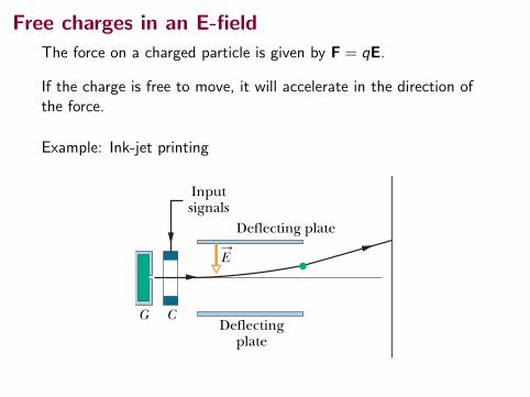
Free charges in an E-field
The force on a charged particle is given by F = qE.
If the charge is free to move, it will accelerate in the direction ofthe force.
Example: Ink-jet printing
Inputsignals
Deflecting plate
G CDeflecting
plate
E
592 CHAPTE R 22 E LECTR IC F I E LDS
The electrostatic force acting on a charged particle located in an external electricfield has the direction of if the charge q of the particle is positive and has theopposite direction if q is negative.
E:
E:
F:
CHECKPOINT 3
(a) In the figure, what is the direction ofthe electrostatic force on the electrondue to the external electric field shown?(b) In which direction will the electronaccelerate if it is moving parallel to the yaxis before it encounters the externalfield? (c) If, instead, the electron is ini-tially moving rightward, will its speedincrease, decrease, or remain constant?
xe
y
E
Fig. 22-14 The Millikan oil-drop appa-ratus for measuring the elementary chargee.When a charged oil drop drifted intochamber C through the hole in plate P1, itsmotion could be controlled by closing andopening switch S and thereby setting up oreliminating an electric field in chamber C.The microscope was used to view the drop,to permit timing of its motion.
Fig. 22-15 Ink-jet printer. Drops shotfrom generator G receive a charge incharging unit C.An input signal from acomputer controls the charge and thus theeffect of field on where the drop lands onthe paper.
E:
22-8 A Point Charge in an Electric FieldIn the preceding four sections we worked at the first of our two tasks: given acharge distribution, to find the electric field it produces in the surrounding space.Here we begin the second task: to determine what happens to a charged particlewhen it is in an electric field set up by other stationary or slowly moving charges.
What happens is that an electrostatic force acts on the particle, as given by
(22-28)
in which q is the charge of the particle (including its sign) and is the electricfield that other charges have produced at the location of the particle. (The field isnot the field set up by the particle itself; to distinguish the two fields, the fieldacting on the particle in Eq. 22-28 is often called the external field. A chargedparticle or object is not affected by its own electric field.) Equation 22-28 tells us
E:
F:
! qE:
,
Measuring the Elementary ChargeEquation 22-28 played a role in the measurement of the elementary charge e byAmerican physicist Robert A. Millikan in 1910–1913. Figure 22-14 is a represen-tation of his apparatus. When tiny oil drops are sprayed into chamber A, some ofthem become charged, either positively or negatively, in the process. Consider adrop that drifts downward through the small hole in plate P1 and into chamber C.Let us assume that this drop has a negative charge q.
If switch S in Fig. 22-14 is open as shown, battery B has no electrical effect onchamber C. If the switch is closed (the connection between chamber C and thepositive terminal of the battery is then complete), the battery causes an excesspositive charge on conducting plate P1 and an excess negative charge on conduct-ing plate P2. The charged plates set up a downward-directed electric field inchamber C. According to Eq. 22-28, this field exerts an electrostatic force on anycharged drop that happens to be in the chamber and affects its motion. In partic-ular, our negatively charged drop will tend to drift upward.
By timing the motion of oil drops with the switch opened and with it closedand thus determining the effect of the charge q, Millikan discovered that thevalues of q were always given by
q ! ne, for n ! 0, "1, "2, "3, . . . , (22-29)
in which e turned out to be the fundamental constant we call the elementarycharge, 1.60 # 10$19 C. Millikan’s experiment is convincing proof that charge isquantized, and he earned the 1923 Nobel Prize in physics in part for this work.Modern measurements of the elementary charge rely on a variety of interlockingexperiments, all more precise than the pioneering experiment of Millikan.
Ink-Jet PrintingThe need for high-quality, high-speed printing has caused a search for analternative to impact printing, such as occurs in a standard typewriter. Buildingup letters by squirting tiny drops of ink at the paper is one such alternative.
Figure 22-15 shows a negatively charged drop moving between two conduct-ing deflecting plates, between which a uniform, downward-directed electric field
has been set up. The drop is deflected upward according to Eq. 22-28 and thenE:
E:
Insulatingchamberwall
+ –B
S
P2
COildrop
P1
A
Microscope
Oilspray
halliday_c22_580-604hr.qxd 7-12-2009 14:16 Page 592

Motion of a Charged Particle in an E-field
712 Chapter 23 Electric Fields
Example 23.11 An Accelerated Electron
An electron enters the region of a uniform electric field as shown in Figure 23.24, with vi 5 3.00 3 106 m/s and E 5 200 N/C. The horizontal length of the plates is , 5 0.100 m.
(A) Find the acceleration of the electron while it is in the elec-tric field.
Conceptualize This example differs from the preceding one because the velocity of the charged particle is initially perpen-dicular to the electric field lines. (In Example 23.10, the veloc-ity of the charged particle is always parallel to the electric field lines.) As a result, the electron in this example follows a curved path as shown in Figure 23.24. The motion of the electron is the same as that of a massive particle projected horizontally in a gravitational field near the surface of the Earth.
Categorize The electron is a particle in a field (electric). Because the electric field is uniform, a constant electric force is exerted on the electron. To find the acceleration of the electron, we can model it as a particle under a net force.
Analyze From the particle in a field model, we know that the direction of the electric force on the electron is down-ward in Figure 23.24, opposite the direction of the electric field lines. From the particle under a net force model, therefore, the acceleration of the electron is downward.
AM
S O L U T I O N
Replace the work and kinetic energies with values appro-priate for this situation:
Fe Dx 5 K ! 2 K " 5 12mvf
2 2 0 S vf 5 Å2Fe Dxm
Analyze Write the appropriate reduction of the conser-vation of energy equation, Equation 8.2, for the system of the charged particle:
W 5 DK
Substitute for the magnitude of the electric force Fe from the particle in a field model and the displacement Dx:
vf 5 Å2 1qE 2 1d 2m
5 Å2qEdm
Finalize The answer to part (B) is the same as that for part (A), as we expect. This problem can be solved with different approaches. We saw the same possibilities with mechanical problems.
(0, 0)
!
(x, y)
vi i!
!vS
x
y
The electron undergoes a downward acceleration (opposite E), and its motion is parabolic while it is between the plates.
S
ES
" " " " " " " " " " " "
! ! ! ! ! ! ! ! ! ! ! !
Figure 23.24 (Example 23.11) An electron is pro-jected horizontally into a uniform electric field pro-duced by two charged plates.
Substitute numerical values: ay 5 211.60 3 10219 C 2 1200 N/C 2
9.11 3 10231 kg5 23.51 3 1013 m/s2
The particle under a net force model was used to develop Equation 23.12 in the case in which the electric force on a particle is the only force. Use this equation to evaluate the y component of the acceleration of the electron:
ay 5 2eEme
(B) Assuming the electron enters the field at time t 5 0, find the time at which it leaves the field.
Categorize Because the electric force acts only in the vertical direction in Figure 23.24, the motion of the particle in the horizontal direction can be analyzed by modeling it as a particle under constant velocity.
S O L U T I O N
▸ 23.10 c o n t i n u e d
Trajectory is a parabola: similar to projectile motion.

Motion of a Charged Particle in an E-field(a) What is the acceleration of an electron in the field of strengthE?
712 Chapter 23 Electric Fields
Example 23.11 An Accelerated Electron
An electron enters the region of a uniform electric field as shown in Figure 23.24, with vi 5 3.00 3 106 m/s and E 5 200 N/C. The horizontal length of the plates is , 5 0.100 m.
(A) Find the acceleration of the electron while it is in the elec-tric field.
Conceptualize This example differs from the preceding one because the velocity of the charged particle is initially perpen-dicular to the electric field lines. (In Example 23.10, the veloc-ity of the charged particle is always parallel to the electric field lines.) As a result, the electron in this example follows a curved path as shown in Figure 23.24. The motion of the electron is the same as that of a massive particle projected horizontally in a gravitational field near the surface of the Earth.
Categorize The electron is a particle in a field (electric). Because the electric field is uniform, a constant electric force is exerted on the electron. To find the acceleration of the electron, we can model it as a particle under a net force.
Analyze From the particle in a field model, we know that the direction of the electric force on the electron is down-ward in Figure 23.24, opposite the direction of the electric field lines. From the particle under a net force model, therefore, the acceleration of the electron is downward.
AM
S O L U T I O N
Replace the work and kinetic energies with values appro-priate for this situation:
Fe Dx 5 K ! 2 K " 5 12mvf
2 2 0 S vf 5 Å2Fe Dxm
Analyze Write the appropriate reduction of the conser-vation of energy equation, Equation 8.2, for the system of the charged particle:
W 5 DK
Substitute for the magnitude of the electric force Fe from the particle in a field model and the displacement Dx:
vf 5 Å2 1qE 2 1d 2m
5 Å2qEdm
Finalize The answer to part (B) is the same as that for part (A), as we expect. This problem can be solved with different approaches. We saw the same possibilities with mechanical problems.
(0, 0)
!
(x, y)
vi i!
!vS
x
y
The electron undergoes a downward acceleration (opposite E), and its motion is parabolic while it is between the plates.
S
ES
" " " " " " " " " " " "
! ! ! ! ! ! ! ! ! ! ! !
Figure 23.24 (Example 23.11) An electron is pro-jected horizontally into a uniform electric field pro-duced by two charged plates.
Substitute numerical values: ay 5 211.60 3 10219 C 2 1200 N/C 2
9.11 3 10231 kg5 23.51 3 1013 m/s2
The particle under a net force model was used to develop Equation 23.12 in the case in which the electric force on a particle is the only force. Use this equation to evaluate the y component of the acceleration of the electron:
ay 5 2eEme
(B) Assuming the electron enters the field at time t 5 0, find the time at which it leaves the field.
Categorize Because the electric force acts only in the vertical direction in Figure 23.24, the motion of the particle in the horizontal direction can be analyzed by modeling it as a particle under constant velocity.
S O L U T I O N
▸ 23.10 c o n t i n u e d
(b) The charge leaves the field at the point (`, yf ). What is yf interms of `, vi ,E , e, and me?
yf = −eE `2
2mev2i

Trick for working out Net field
Look for symmetry in the problem.
To find the E-field, usually several components (Ex , Ey , Ex) mustbe found independently.
If the effects of charges will cancel out, you can neglect thosecharges.
If the effects of charges cancel out in one component, just worryabout the other component(s).

Question about net field
597QU E STION SPART 3
1 Figure 22-20 shows three arrangements of electric field lines. Ineach arrangement, a proton is released from rest at point A and isthen accelerated through point B by the electric field. Points A andB have equal separations in the three arrangements. Rank thearrangements according to the linear momentum of the proton atpoint B, greatest first.
ducing it? (c) Is the magnitude ofthe net electric field at P equal tothe sum of the magnitudes E of thetwo field vectors (is it equal to2E)? (d) Do the x components ofthose two field vectors add or can-cel? (e) Do their y componentsadd or cancel? (f) Is the directionof the net field at P that of the can-celing components or the adding components? (g) What is the di-rection of the net field?
4 Figure 22-23 shows four situations in which four charged parti-cles are evenly spaced to the left and right of a central point. Thecharge values are indicated. Rank the situations according to themagnitude of the net electric field at the central point, greatest first.
A B A B A B
(a) (b) (c)
Fig. 22-20 Question 1.
2 Figure 22-21 shows two square arrays of charged particles. Thesquares, which are centered on point P, are misaligned. The parti-cles are separated by either d or d/2 along the perimeters of thesquares. What are the magnitude and direction of the net electricfield at P?
+6q
–2q
+3q–2q
+3q
–q
+6q
–2q
–3q
–q
+2q –3q
+2q
–qP
Fig. 22-21 Question 2.
where z is the distance between the point and the center of thedipole.
Field Due to a Continuous Charge Distribution Theelectric field due to a continuous charge distribution is found bytreating charge elements as point charges and then summing, viaintegration, the electric field vectors produced by all the charge el-ements to find the net vector.
Force on a Point Charge in an Electric Field When apoint charge q is placed in an external electric field , the electro-static force that acts on the point charge is
. (22-28)F:
! qE:
F:
E:
Force has the same direction as if q is positive and theopposite direction if q is negative.
Dipole in an Electric Field When an electric dipole of dipolemoment is placed in an electric field , the field exerts a torque
on the dipole:(22-34)
The dipole has a potential energy U associated with its orientationin the field:
(22-38)
This potential energy is defined to be zero when is perpendicularto ; it is least ( ) when is aligned with and greatest( ) when is directed opposite .E
:p:U ! pE
E:
p:U ! "pEE:
p:U ! "p: ! E
:.
#: ! p: " E:
.#:
E:
p:
E:
F:
3 In Fig. 22-22, two particles of charge "q are arranged symmet-rically about the y axis; each produces an electric field at point P onthat axis. (a) Are the magnitudes of the fields at P equal? (b) Iseach electric field directed toward or away from the charge pro-
x
y
P
–q –q
d d
Fig. 22-22 Question 3.
(1)+e +e–e –e
(2)+e –e+e –e
(3)–e +e+e +e
(4)–e –e –e+e
d d d d
Fig. 22-23 Question 4.
5 Figure 22-24 shows two charged particles fixed in place on anaxis. (a) Where on the axis (otherthan at an infinite distance) is therea point at which their net electricfield is zero: between the charges, totheir left, or to their right? (b) Isthere a point of zero net electric fieldanywhere off the axis (other than atan infinite distance)?
6 In Fig. 22-25, two identical cir-cular nonconducting rings are cen-
+q –3q
Fig. 22-24 Question 5.
P1 P2 P3
Ring A Ring B
Fig. 22-25 Question 6.
halliday_c22_580-604hr.qxd 7-12-2009 14:16 Page 597
** View All Solutions Here **
** View All Solutions Here **
1Figure from Halliday, Resnick, Walker, page 597, problem 2.

Electric Dipole
electric dipole
A pair of charges of equal magnitude q but opposite sign,separated by a distance, d .
dipole moment:
p = qd r
where r is a unit vector pointing from the negative charge to thepositive charge.
584 CHAPTE R 22 E LECTR IC F I E LDS
Fig. 22-8 (a) An electric dipole.Theelectric field vectors and at pointP on the dipole axis result from the dipole’stwo charges. Point P is at distances r(!) andr(") from the individual charges that makeup the dipole. (b) The dipole moment ofthe dipole points from the negative chargeto the positive charge.
p:
E:
(")E:
(!)
z
r(–)
r(+)
E(+)
d
z
–q
+q
P
(a) (b)
+ +
– –
p
E(–)
Dipole center
Up here the +qfield dominates.
Down here the –qfield dominates.
22-5 The Electric Field Due to an Electric DipoleFigure 22-8a shows two charged particles of magnitude q but of opposite sign,separated by a distance d. As was noted in connection with Fig. 22-5, we call thisconfiguration an electric dipole. Let us find the electric field due to the dipole ofFig. 22-8a at a point P, a distance z from the midpoint of the dipole and on theaxis through the particles, which is called the dipole axis.
From symmetry, the electric field at point P—and also the fields andE:
(") due to the separate charges that make up the dipole—must lie along thedipole axis, which we have taken to be a z axis.Applying the superposition princi-ple for electric fields, we find that the magnitude E of the electric field at P is
(22-5)
After a little algebra, we can rewrite this equation as
(22-6)
After forming a common denominator and multiplying its terms, we come to
(22-7)
We are usually interested in the electrical effect of a dipole only at distancesthat are large compared with the dimensions of the dipole—that is, at distances suchthat z # d. At such large distances, we have d/2z $ 1 in Eq. 22-7. Thus, in our ap-proximation, we can neglect the d/2z term in the denominator, which leaves us with
(22-8)
The product qd, which involves the two intrinsic properties q and d of thedipole, is the magnitude p of a vector quantity known as the electric dipole moment
of the dipole. (The unit of is the coulomb-meter.) Thus, we can write Eq. 22-8 as
(electric dipole). (22-9)
The direction of is taken to be from the negative to the positive end of thedipole, as indicated in Fig. 22-8b. We can use the direction of to specify theorientation of a dipole.
Equation 22-9 shows that, if we measure the electric field of a dipole only atdistant points, we can never find q and d separately; instead, we can find only theirproduct. The field at distant points would be unchanged if, for example, q weredoubled and d simultaneously halved. Although Eq. 22-9 holds only for distantpoints along the dipole axis, it turns out that E for a dipole varies as 1/r 3 for alldistant points, regardless of whether they lie on the dipole axis; here r is the dis-tance between the point in question and the dipole center.
Inspection of Fig. 22-8 and of the field lines in Fig. 22-5 shows that the direc-tion of for distant points on the dipole axis is always the direction of the dipoleE
:
p:p:
E %1
2&'0
pz3
p:p:
E %1
2&'0 qdz3 .
%q
2&'0z3 d
!1 " ! d2z "
2"2 .E %q
4&'0z2 2d/z
!1 " ! d2z "
2"2
E %q
4&'0z2 ! 1
!1 "d2z "
2 "1
!1 ! d2z "
2 ".
%q
4&'0(z " 12d)2 "
q4&'0(z ! 1
2d)2 .
%1
4&'0
qr2
(!)"
14&'0
q
r2(")
E % E(!) " E(")
E:
(!)E:
halliday_c22_580-604hr.qxd 7-12-2009 14:16 Page 584

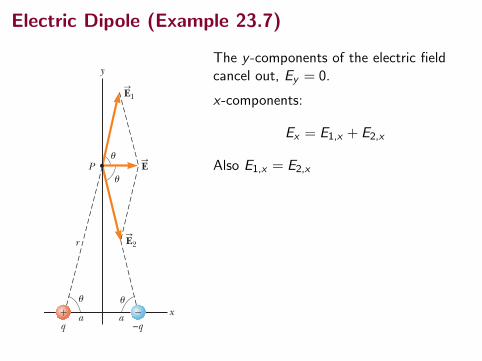
Electric Dipole (Example 23.6, B)Evaluate the electric field from the dipole at point P, which is atposition (0, y).
23.4 Analysis Model: Particle in a Field (Electric) 703
(B) Evaluate the electric field at point P in the special case that uq1u 5 uq2u and a 5 b.
Conceptualize Figure 23.13 shows the situation in this special case. Notice the symmetry in the situa-tion and that the charge distribution is now an elec-tric dipole.
Categorize Because Figure 23.13 is a special case of the general case shown in Figure 23.12, we can cat-egorize this example as one in which we can take the result of part (A) and substitute the appropriate val-ues of the variables.
S O L U T I O N
P
y
r
aq
a–q
x
u
u
u u
! "
ES
E2S
E1S
Figure 23.13 (Example 23.6) When the charges in Figure 23.12 are of equal magnitude and equidistant from the origin, the situation becomes symmet-ric as shown here.
Analyze Based on the symmetry in Figure 23.13, evaluate Equations (1) and (2) from part (A) with a 5 b, uq1u 5 uq2u 5 q, and f 5 u:
(3) Ex 5 ke q
a 2 1 y 2 cos u 1 ke q
a 2 1 y 2 cos u 5 2ke q
a 2 1 y2 cos u
Ey 5 ke q
a 2 1 y 2 sin u 2 ke q
a 2 1 y 2 sin u 5 0
From the geometry in Figure 23.13, evaluate cos u:
(4) cos u 5ar
5a1a 2 1 y 2 21/2
Substitute Equation (4) into Equation (3): Ex 5 2ke q
a 2 1 y 2 c a1a 2 1 y 2 21/2 d 5 ke 2aq1a 2 1 y 2 23/2
(C) Find the electric field due to the electric dipole when point P is a distance y .. a from the origin.
S O L U T I O N
In the solution to part (B), because y .. a, neglect a2 com-pared with y 2 and write the expression for E in this case:
(5) E < ke 2aq
y 3
Write the components of the net electric field vector:
(1) Ex 5 E1x 1 E 2x 5 ke 0 q1 0
a 2 1 y 2 cos f 1 ke 0 q 2 0
b 2 1 y 2 cos u
(2) Ey 5 E 1y 1 E 2y 5 ke 0 q1 0
a 2 1 y 2 sin f 2 ke 0 q2 0
b 2 1 y 2 sin u
▸ 23.6 c o n t i n u e d
Finalize From Equation (5), we see that at points far from a dipole but along the perpendicular bisector of the line joining the two charges, the magnitude of the electric field created by the dipole varies as 1/r 3, whereas the more slowly varying field of a point charge varies as 1/r 2 (see Eq. 23.9). That is because at distant points, the fields of the two charges of equal magnitude and opposite sign almost cancel each other. The 1/r 3 variation in E for the dipole also is obtained for a distant point along the x axis and for any general distant point.
Electric Dipole (Example 23.7)
23.4 Analysis Model: Particle in a Field (Electric) 703
(B) Evaluate the electric field at point P in the special case that uq1u 5 uq2u and a 5 b.
Conceptualize Figure 23.13 shows the situation in this special case. Notice the symmetry in the situa-tion and that the charge distribution is now an elec-tric dipole.
Categorize Because Figure 23.13 is a special case of the general case shown in Figure 23.12, we can cat-egorize this example as one in which we can take the result of part (A) and substitute the appropriate val-ues of the variables.
S O L U T I O N
P
y
r
aq
a–q
x
u
u
u u
! "
ES
E2S
E1S
Figure 23.13 (Example 23.6) When the charges in Figure 23.12 are of equal magnitude and equidistant from the origin, the situation becomes symmet-ric as shown here.
Analyze Based on the symmetry in Figure 23.13, evaluate Equations (1) and (2) from part (A) with a 5 b, uq1u 5 uq2u 5 q, and f 5 u:
(3) Ex 5 ke q
a 2 1 y 2 cos u 1 ke q
a 2 1 y 2 cos u 5 2ke q
a 2 1 y2 cos u
Ey 5 ke q
a 2 1 y 2 sin u 2 ke q
a 2 1 y 2 sin u 5 0
From the geometry in Figure 23.13, evaluate cos u:
(4) cos u 5ar
5a1a 2 1 y 2 21/2
Substitute Equation (4) into Equation (3): Ex 5 2ke q
a 2 1 y 2 c a1a 2 1 y 2 21/2 d 5 ke 2aq1a 2 1 y 2 23/2
(C) Find the electric field due to the electric dipole when point P is a distance y .. a from the origin.
S O L U T I O N
In the solution to part (B), because y .. a, neglect a2 com-pared with y 2 and write the expression for E in this case:
(5) E < ke 2aq
y 3
Write the components of the net electric field vector:
(1) Ex 5 E1x 1 E 2x 5 ke 0 q1 0
a 2 1 y 2 cos f 1 ke 0 q 2 0
b 2 1 y 2 cos u
(2) Ey 5 E 1y 1 E 2y 5 ke 0 q1 0
a 2 1 y 2 sin f 2 ke 0 q2 0
b 2 1 y 2 sin u
▸ 23.6 c o n t i n u e d
Finalize From Equation (5), we see that at points far from a dipole but along the perpendicular bisector of the line joining the two charges, the magnitude of the electric field created by the dipole varies as 1/r 3, whereas the more slowly varying field of a point charge varies as 1/r 2 (see Eq. 23.9). That is because at distant points, the fields of the two charges of equal magnitude and opposite sign almost cancel each other. The 1/r 3 variation in E for the dipole also is obtained for a distant point along the x axis and for any general distant point.
The y -components of the electric fieldcancel out, Ey = 0.
x-components:
Ex = E1,x + E2,x
Also E1,x = E2,x
Ex = 2
(ke q
r2cos θ
)
=2ke q
(a2 + y2)
(a√
a2 + y2
)
=2ke a q
(a2 + y2)3/2
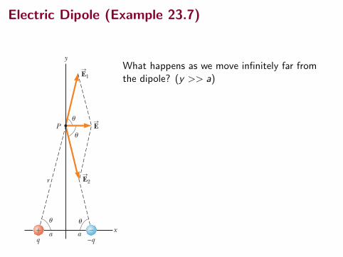
Electric Dipole (Example 23.7)
23.4 Analysis Model: Particle in a Field (Electric) 703
(B) Evaluate the electric field at point P in the special case that uq1u 5 uq2u and a 5 b.
Conceptualize Figure 23.13 shows the situation in this special case. Notice the symmetry in the situa-tion and that the charge distribution is now an elec-tric dipole.
Categorize Because Figure 23.13 is a special case of the general case shown in Figure 23.12, we can cat-egorize this example as one in which we can take the result of part (A) and substitute the appropriate val-ues of the variables.
S O L U T I O N
P
y
r
aq
a–q
x
u
u
u u
! "
ES
E2S
E1S
Figure 23.13 (Example 23.6) When the charges in Figure 23.12 are of equal magnitude and equidistant from the origin, the situation becomes symmet-ric as shown here.
Analyze Based on the symmetry in Figure 23.13, evaluate Equations (1) and (2) from part (A) with a 5 b, uq1u 5 uq2u 5 q, and f 5 u:
(3) Ex 5 ke q
a 2 1 y 2 cos u 1 ke q
a 2 1 y 2 cos u 5 2ke q
a 2 1 y2 cos u
Ey 5 ke q
a 2 1 y 2 sin u 2 ke q
a 2 1 y 2 sin u 5 0
From the geometry in Figure 23.13, evaluate cos u:
(4) cos u 5ar
5a1a 2 1 y 2 21/2
Substitute Equation (4) into Equation (3): Ex 5 2ke q
a 2 1 y 2 c a1a 2 1 y 2 21/2 d 5 ke 2aq1a 2 1 y 2 23/2
(C) Find the electric field due to the electric dipole when point P is a distance y .. a from the origin.
S O L U T I O N
In the solution to part (B), because y .. a, neglect a2 com-pared with y 2 and write the expression for E in this case:
(5) E < ke 2aq
y 3
Write the components of the net electric field vector:
(1) Ex 5 E1x 1 E 2x 5 ke 0 q1 0
a 2 1 y 2 cos f 1 ke 0 q 2 0
b 2 1 y 2 cos u
(2) Ey 5 E 1y 1 E 2y 5 ke 0 q1 0
a 2 1 y 2 sin f 2 ke 0 q2 0
b 2 1 y 2 sin u
▸ 23.6 c o n t i n u e d
Finalize From Equation (5), we see that at points far from a dipole but along the perpendicular bisector of the line joining the two charges, the magnitude of the electric field created by the dipole varies as 1/r 3, whereas the more slowly varying field of a point charge varies as 1/r 2 (see Eq. 23.9). That is because at distant points, the fields of the two charges of equal magnitude and opposite sign almost cancel each other. The 1/r 3 variation in E for the dipole also is obtained for a distant point along the x axis and for any general distant point.
What happens as we move infinitely far fromthe dipole? (y >> a)
The constant a in the denominator has lessand less affect on the function. We can seethat the field function approaches Efar =
2ke a qy3
limy→∞
[E
Efar
]= lim
y→∞ 2ke a q
(a2+y2)3/2
2ke a qy3
=
= 1

Electric Dipole (Example 23.7)
23.4 Analysis Model: Particle in a Field (Electric) 703
(B) Evaluate the electric field at point P in the special case that uq1u 5 uq2u and a 5 b.
Conceptualize Figure 23.13 shows the situation in this special case. Notice the symmetry in the situa-tion and that the charge distribution is now an elec-tric dipole.
Categorize Because Figure 23.13 is a special case of the general case shown in Figure 23.12, we can cat-egorize this example as one in which we can take the result of part (A) and substitute the appropriate val-ues of the variables.
S O L U T I O N
P
y
r
aq
a–q
x
u
u
u u
! "
ES
E2S
E1S
Figure 23.13 (Example 23.6) When the charges in Figure 23.12 are of equal magnitude and equidistant from the origin, the situation becomes symmet-ric as shown here.
Analyze Based on the symmetry in Figure 23.13, evaluate Equations (1) and (2) from part (A) with a 5 b, uq1u 5 uq2u 5 q, and f 5 u:
(3) Ex 5 ke q
a 2 1 y 2 cos u 1 ke q
a 2 1 y 2 cos u 5 2ke q
a 2 1 y2 cos u
Ey 5 ke q
a 2 1 y 2 sin u 2 ke q
a 2 1 y 2 sin u 5 0
From the geometry in Figure 23.13, evaluate cos u:
(4) cos u 5ar
5a1a 2 1 y 2 21/2
Substitute Equation (4) into Equation (3): Ex 5 2ke q
a 2 1 y 2 c a1a 2 1 y 2 21/2 d 5 ke 2aq1a 2 1 y 2 23/2
(C) Find the electric field due to the electric dipole when point P is a distance y .. a from the origin.
S O L U T I O N
In the solution to part (B), because y .. a, neglect a2 com-pared with y 2 and write the expression for E in this case:
(5) E < ke 2aq
y 3
Write the components of the net electric field vector:
(1) Ex 5 E1x 1 E 2x 5 ke 0 q1 0
a 2 1 y 2 cos f 1 ke 0 q 2 0
b 2 1 y 2 cos u
(2) Ey 5 E 1y 1 E 2y 5 ke 0 q1 0
a 2 1 y 2 sin f 2 ke 0 q2 0
b 2 1 y 2 sin u
▸ 23.6 c o n t i n u e d
Finalize From Equation (5), we see that at points far from a dipole but along the perpendicular bisector of the line joining the two charges, the magnitude of the electric field created by the dipole varies as 1/r 3, whereas the more slowly varying field of a point charge varies as 1/r 2 (see Eq. 23.9). That is because at distant points, the fields of the two charges of equal magnitude and opposite sign almost cancel each other. The 1/r 3 variation in E for the dipole also is obtained for a distant point along the x axis and for any general distant point.
What happens as we move infinitely far fromthe dipole? (y >> a)
The constant a in the denominator has lessand less affect on the function. We can seethat the field function approaches Efar =
2ke a qy3
limy→∞
[E
Efar
]= lim
y→∞ 2ke a q
(a2+y2)3/2
2ke a qy3
= limy→∞
2ke a q
y3(( ay )
2+1)3/2
2ke a qy3
= 1
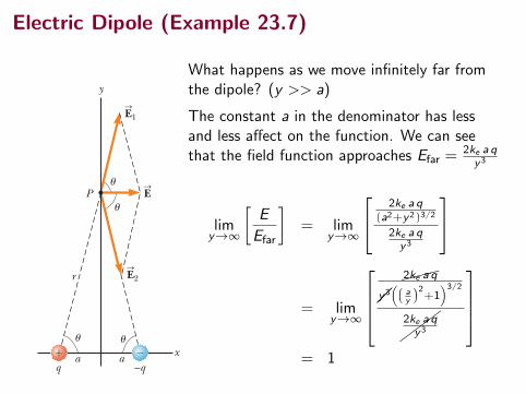
Electric Dipole (Example 23.7)
23.4 Analysis Model: Particle in a Field (Electric) 703
(B) Evaluate the electric field at point P in the special case that uq1u 5 uq2u and a 5 b.
Conceptualize Figure 23.13 shows the situation in this special case. Notice the symmetry in the situa-tion and that the charge distribution is now an elec-tric dipole.
Categorize Because Figure 23.13 is a special case of the general case shown in Figure 23.12, we can cat-egorize this example as one in which we can take the result of part (A) and substitute the appropriate val-ues of the variables.
S O L U T I O N
P
y
r
aq
a–q
x
u
u
u u
! "
ES
E2S
E1S
Figure 23.13 (Example 23.6) When the charges in Figure 23.12 are of equal magnitude and equidistant from the origin, the situation becomes symmet-ric as shown here.
Analyze Based on the symmetry in Figure 23.13, evaluate Equations (1) and (2) from part (A) with a 5 b, uq1u 5 uq2u 5 q, and f 5 u:
(3) Ex 5 ke q
a 2 1 y 2 cos u 1 ke q
a 2 1 y 2 cos u 5 2ke q
a 2 1 y2 cos u
Ey 5 ke q
a 2 1 y 2 sin u 2 ke q
a 2 1 y 2 sin u 5 0
From the geometry in Figure 23.13, evaluate cos u:
(4) cos u 5ar
5a1a 2 1 y 2 21/2
Substitute Equation (4) into Equation (3): Ex 5 2ke q
a 2 1 y 2 c a1a 2 1 y 2 21/2 d 5 ke 2aq1a 2 1 y 2 23/2
(C) Find the electric field due to the electric dipole when point P is a distance y .. a from the origin.
S O L U T I O N
In the solution to part (B), because y .. a, neglect a2 com-pared with y 2 and write the expression for E in this case:
(5) E < ke 2aq
y 3
Write the components of the net electric field vector:
(1) Ex 5 E1x 1 E 2x 5 ke 0 q1 0
a 2 1 y 2 cos f 1 ke 0 q 2 0
b 2 1 y 2 cos u
(2) Ey 5 E 1y 1 E 2y 5 ke 0 q1 0
a 2 1 y 2 sin f 2 ke 0 q2 0
b 2 1 y 2 sin u
▸ 23.6 c o n t i n u e d
Finalize From Equation (5), we see that at points far from a dipole but along the perpendicular bisector of the line joining the two charges, the magnitude of the electric field created by the dipole varies as 1/r 3, whereas the more slowly varying field of a point charge varies as 1/r 2 (see Eq. 23.9). That is because at distant points, the fields of the two charges of equal magnitude and opposite sign almost cancel each other. The 1/r 3 variation in E for the dipole also is obtained for a distant point along the x axis and for any general distant point.
What happens as we move infinitely far fromthe dipole? (y >> a)
The constant a in the denominator has lessand less affect on the function. We can seethat the field function approaches Efar =
2ke a qy3
limy→∞
[E
Efar
]= lim
y→∞ 2ke a q
(a2+y2)3/2
2ke a qy3
= limy→∞
���2ke a q
��y3(( ay )
2+1)3/2
���2ke a q
y3
= 1

Big-O Notation (Example 23.7)
23.4 Analysis Model: Particle in a Field (Electric) 703
(B) Evaluate the electric field at point P in the special case that uq1u 5 uq2u and a 5 b.
Conceptualize Figure 23.13 shows the situation in this special case. Notice the symmetry in the situa-tion and that the charge distribution is now an elec-tric dipole.
Categorize Because Figure 23.13 is a special case of the general case shown in Figure 23.12, we can cat-egorize this example as one in which we can take the result of part (A) and substitute the appropriate val-ues of the variables.
S O L U T I O N
P
y
r
aq
a–q
x
u
u
u u
! "
ES
E2S
E1S
Figure 23.13 (Example 23.6) When the charges in Figure 23.12 are of equal magnitude and equidistant from the origin, the situation becomes symmet-ric as shown here.
Analyze Based on the symmetry in Figure 23.13, evaluate Equations (1) and (2) from part (A) with a 5 b, uq1u 5 uq2u 5 q, and f 5 u:
(3) Ex 5 ke q
a 2 1 y 2 cos u 1 ke q
a 2 1 y 2 cos u 5 2ke q
a 2 1 y2 cos u
Ey 5 ke q
a 2 1 y 2 sin u 2 ke q
a 2 1 y 2 sin u 5 0
From the geometry in Figure 23.13, evaluate cos u:
(4) cos u 5ar
5a1a 2 1 y 2 21/2
Substitute Equation (4) into Equation (3): Ex 5 2ke q
a 2 1 y 2 c a1a 2 1 y 2 21/2 d 5 ke 2aq1a 2 1 y 2 23/2
(C) Find the electric field due to the electric dipole when point P is a distance y .. a from the origin.
S O L U T I O N
In the solution to part (B), because y .. a, neglect a2 com-pared with y 2 and write the expression for E in this case:
(5) E < ke 2aq
y 3
Write the components of the net electric field vector:
(1) Ex 5 E1x 1 E 2x 5 ke 0 q1 0
a 2 1 y 2 cos f 1 ke 0 q 2 0
b 2 1 y 2 cos u
(2) Ey 5 E 1y 1 E 2y 5 ke 0 q1 0
a 2 1 y 2 sin f 2 ke 0 q2 0
b 2 1 y 2 sin u
▸ 23.6 c o n t i n u e d
Finalize From Equation (5), we see that at points far from a dipole but along the perpendicular bisector of the line joining the two charges, the magnitude of the electric field created by the dipole varies as 1/r 3, whereas the more slowly varying field of a point charge varies as 1/r 2 (see Eq. 23.9). That is because at distant points, the fields of the two charges of equal magnitude and opposite sign almost cancel each other. The 1/r 3 variation in E for the dipole also is obtained for a distant point along the x axis and for any general distant point.
y >> a
Recall that f (x) = O(g(x)) if∣∣∣ f (x)g(x)
∣∣∣ 6 C
∀ x > k .
∣∣∣∣ E
Efar
∣∣∣∣ =
∣∣∣∣∣∣2ke a q
(a2+y2)3/2
2ke a qy3
∣∣∣∣∣∣=
∣∣∣∣∣∣((
a
y
)2
+ 1
)−3/2∣∣∣∣∣∣
Choosing k = a we can see:∣∣∣∣ E
Efar
∣∣∣∣ 61
2√
2∀ y > a
Therefore, E = O(2ke a qy3
)or simply O(y−3).

Big-O Notation (Example 23.7)
23.4 Analysis Model: Particle in a Field (Electric) 703
(B) Evaluate the electric field at point P in the special case that uq1u 5 uq2u and a 5 b.
Conceptualize Figure 23.13 shows the situation in this special case. Notice the symmetry in the situa-tion and that the charge distribution is now an elec-tric dipole.
Categorize Because Figure 23.13 is a special case of the general case shown in Figure 23.12, we can cat-egorize this example as one in which we can take the result of part (A) and substitute the appropriate val-ues of the variables.
S O L U T I O N
P
y
r
aq
a–q
x
u
u
u u
! "
ES
E2S
E1S
Figure 23.13 (Example 23.6) When the charges in Figure 23.12 are of equal magnitude and equidistant from the origin, the situation becomes symmet-ric as shown here.
Analyze Based on the symmetry in Figure 23.13, evaluate Equations (1) and (2) from part (A) with a 5 b, uq1u 5 uq2u 5 q, and f 5 u:
(3) Ex 5 ke q
a 2 1 y 2 cos u 1 ke q
a 2 1 y 2 cos u 5 2ke q
a 2 1 y2 cos u
Ey 5 ke q
a 2 1 y 2 sin u 2 ke q
a 2 1 y 2 sin u 5 0
From the geometry in Figure 23.13, evaluate cos u:
(4) cos u 5ar
5a1a 2 1 y 2 21/2
Substitute Equation (4) into Equation (3): Ex 5 2ke q
a 2 1 y 2 c a1a 2 1 y 2 21/2 d 5 ke 2aq1a 2 1 y 2 23/2
(C) Find the electric field due to the electric dipole when point P is a distance y .. a from the origin.
S O L U T I O N
In the solution to part (B), because y .. a, neglect a2 com-pared with y 2 and write the expression for E in this case:
(5) E < ke 2aq
y 3
Write the components of the net electric field vector:
(1) Ex 5 E1x 1 E 2x 5 ke 0 q1 0
a 2 1 y 2 cos f 1 ke 0 q 2 0
b 2 1 y 2 cos u
(2) Ey 5 E 1y 1 E 2y 5 ke 0 q1 0
a 2 1 y 2 sin f 2 ke 0 q2 0
b 2 1 y 2 sin u
▸ 23.6 c o n t i n u e d
Finalize From Equation (5), we see that at points far from a dipole but along the perpendicular bisector of the line joining the two charges, the magnitude of the electric field created by the dipole varies as 1/r 3, whereas the more slowly varying field of a point charge varies as 1/r 2 (see Eq. 23.9). That is because at distant points, the fields of the two charges of equal magnitude and opposite sign almost cancel each other. The 1/r 3 variation in E for the dipole also is obtained for a distant point along the x axis and for any general distant point.
y >> a
Recall that f (x) = O(g(x)) if∣∣∣ f (x)g(x)
∣∣∣ 6 C
∀ x > k .∣∣∣∣ E
Efar
∣∣∣∣ =
∣∣∣∣∣∣2ke a q
(a2+y2)3/2
2ke a qy3
∣∣∣∣∣∣=
∣∣∣∣∣∣((
a
y
)2
+ 1
)−3/2∣∣∣∣∣∣
Choosing k = a we can see:∣∣∣∣ E
Efar
∣∣∣∣ 61
2√
2∀ y > a
Therefore, E = O(2ke a qy3
)or simply O(y−3).

Electric Dipole (Example 23.7)
As we move away from the dipole (red line, r−3) the E-field fallsoff faster than it does for a point charge (blue line, r−2).
The negative charge partially shields the effect of the positivecharge and vice versa.

Summary
• electric field lines
• the effect of fields on charges
• the electric dipole
Homework• Collected homework 1, posted online, due on Monday, Jan 22.
Serway & Jewett:
• NEW: Ch 23, onward from page 716. Probs: 36, 51, 61, 79
• Understand examples 23.8 and 23.9.