ii

DOE Award No.: DE-FC26-06NT42959

Final Report

“Electrical Resistivity Investigation of Gas Hydrate Distribution in Mississippi Canyon

Block 118, Gulf of Mexico”

Submitted by: Baylor University

One Bear Place 97354 Waco, Texas 76798

Prepared for:

Office of Fossil Energy

iii

U.S. Department of Energy Title Page Form Maker v1.0 Report Title:

Electrical Resistivity Investigation of Gas Hydrate Distribution in

Mississippi Canyon Block 118, Gulf of Mexico

Report Type: FINAL Report Period Start Date: 9/1/2006 End Date: 12/31/2012

Principal Author(s): John Dunbar

Report Issue Date: 3/31/2013 DOE Award No.: DE- FC26 - 06NT42959

Submitting Organizations(s) Name & address

Baylor University One Bear Place 7354 Waco, TX 76798

i

iv

Project Summary Page ELECTRICAL RESISTIVITY INVESTIGATION OF GAS HYDRATE DISTRIBUTION IN MISSISSIPPI CANYON BLOCK 118, GULF OF MEXICO DOE Award No.: DE-FC26-06NT42959 Recipient Name: Baylor University, One bear Place 97354, Waco, TX 76798 Award Date: October 1, 2006 Completion Date: December 31, 2012 DOE Award: $253,563 (Cum Actual Budget Period 1 from 10/1/06 to 12/31/12) $253,448 (Cum Actual Funds expended 10/1/06-12/31/12) $115 (Remaining funds in BP 2) Principal Investigator: John Dunbar, Baylor University Type of Report: Final Technical Report Date of Report: March 31, 2013 Reporting Period: October 1, 2006 to December 31, 2012

Disclaimer This report was prepared as an account of work sponsored by an agency of the United States

Government. Neither the United States Government nor any agency thereof, nor any of their employees, makes any warranty, express or implied, or assumes any legal liability or responsibility for the accuracy, completeness, or usefulness of any information, apparatus, product, or process disclosed, or represents that its use would not infringe privately owned rights. Reference herein to any specific commercial product, process, or service by trade name, trademark, manufacturer, or otherwise does not necessarily constitute or imply its endorsement, recommendation, or favoring by the United States Government or any agency thereof. The views and opinions of authors expressed herein do not necessarily state or reflect those of the United States Government or any agency thereof.

ii

v

Abstract Electrical methods offer a geophysical approach for determining the sub-bottom distribution of hydrate in deep marine environments. Methane hydrate is essentially non-conductive. Hence, sediments containing hydrate are more resistive than sediments without hydrates. To date, the controlled source electromagnetic (CSEM) method has been used in marine hydrates studies. This project evaluated an alternative electrical method, direct current resistivity (DCR), for detecting marine hydrates. DCR involves the injection of direct current between two source electrodes and the simultaneous measurement of the electric potential (voltage) between multiple receiver electrodes. The DCR method provides subsurface information comparable to that produced by the CSEM method, but with less sophisticated instrumentation. Because the receivers are simple electrodes, large numbers can be deployed to achieve higher spatial resolution. In this project a prototype seafloor DCR system was developed and used to conduct a reconnaissance survey at a site of known hydrate occurrence in Mississippi Canyon Block 118. The resulting images of sub-bottom resistivities indicate that high-concentration hydrates at the site occur only in the upper 50 m, where deep-seated faults intersect the seafloor. Overall, there was evidence for much less hydrate at the site than previously thought based on available seismic and CSEM data alone.

vi

Table of contents Project Summary Page ................................................................................................................................. iv Abstract ......................................................................................................................................................... v Table of contents ......................................................................................................................................... vi List of Figures .............................................................................................................................................. vii List of Acronyms, Symbols and Abbreviations ........................................................................................... viii Executive summary ...................................................................................................................................... ix 1 Introduction ............................................................................................................................................... 1

1.1 Report Overview ................................................................................................................................. 1 1.2 Project Background ............................................................................................................................. 1 1.3 Collaboration with GOM-HRC ............................................................................................................. 3 1.4 Commercial Collaborators .................................................................................................................. 4 1.5 Project Objectives ............................................................................................................................... 6 1.6 Project Phases ..................................................................................................................................... 6

2 Phase 1: Development and Application of the DCR System ...................................................................... 6 2.1 Development of the seafloor DCR system (Task 1.3) ......................................................................... 6

2.1.1 DCR instrument ............................................................................................................................ 6 2.1.2 Instrument pressure housing ....................................................................................................... 7 2.1.3 Electrode arrays ........................................................................................................................... 8 2.1.4 Tow body ...................................................................................................................................... 9

2.2 Reconnaissance survey of MC 118 (Task 1.5) .................................................................................. 11 2.2.1 Initial attempt in June 2008 ....................................................................................................... 11 2.2.2 Field acquisition June 2009 ........................................................................................................ 11 2.2.3 CRP data processing ................................................................................................................... 12 2.2.3 Interpretations of DCR profiles. ................................................................................................. 17 2.2.4 Evaluation of the validity of DCR inversions. ............................................................................. 18 2.2.5 Discussion of Results of Phase 1 ................................................................................................ 20

3 Phase 2: Reconfiguring the DCR System and 3D Survey (Task 2.1) ......................................................... 21 3.1 Reconfiguration of the DCR system for 3D acquisition ..................................................................... 21 3.2 Attempted 3D DCR survey of MC118 ................................................................................................ 23 3.3 Discussion of Phase 2 failure ............................................................................................................. 23

References .................................................................................................................................................. 24

vii

List of Figures Figure 1.1 Study Site.. ................................................................................................................................... 4 Figure 1.2 Seafloor at MC118.. ..................................................................................................................... 5 Figure 2.1 Deep-tow CRP configuration.. ...................................................................................................... 7 Figure 2.2 DCR system remote control. ........................................................................................................ 8 Figure 2.3 Seafloor electrode arrays ............................................................................................................. 9 Figure 2.4 DCR system mounted to SSD ROV ............................................................................................. 10 Figure 2.5. Resistivity track lines at MC118 ................................................................................................ 13 Figure 2.6. Example inverted resistivity sections ....................................................................................... 17 Figure 2.7. Inversion of forward model data .............................................................................................. 19 Figure 2.8. Superposition of resistivity and seismic data. .......................................................................... 20 Figure 3.1. Titanium receiver electrode.. ................................................................................................... 22

viii

List of Acronyms, Symbols and Abbreviations Ωm Ohm-m µV Micro Volt 2D Two-dimensional 3D Three-dimensional 4D Four-dimension BSR Bottom simulating reflection CSEM Controlled source electromagnetic CRP Continuous resistivity profiling DC Direct current DCR Direct current resistivity EM Electromagnetic GOM-HRC Gulf of Mexico-Hydrate Research Consortium GPS Global positioning system mA Milliamp MC 118 Mississippi Canyon Block 118 mV Millivolt PC Personal computer RS232 Electronics Industries Association common computer interface standard SSD Station Service Device ROV Remotely operated vehicle UTM Universal Transverse Mercator

ix

Executive summary General description of project Electrical methods offer a geophysical approach for determining the sub-bottom distribution of hydrate in deep marine environments. Methane hydrate is essentially non-conductive. Hence, sediments containing hydrate are more resistive than sediments without hydrates. To date, the controlled source electromagnetic (CSEM) method has been used in marine hydrates studies. This project was a pilot study to evaluate the direct current resistivity (DCR) method for use in deep marine methane hydrate investigations as a high-resolution alternative to the CSEM method. Benefits Both CSEM and DCR methods work by driving a pair of source electrodes with an alternating square wave of electric current. The two methods differ in that CSEM receivers consist of both magnetometers and electrodes, whereas DCR uses just electrodes. This means that more sources and receivers can be deployed to achieve higher spatial resolution with the DCR method than is practical using the CSEM method. Furthermore, for some applications, the DCR electrodes can be used interchangeably as receivers or sources. This makes it possible to collect DCR data along a profile by reading different electrode configurations along a fixed electrode array, which makes continuous monitoring feasible. Project Phases The project was conducted in two phases. Phase 1 involved the development of a prototype, seafloor DCR system and the initial application of that system in a reconnaissance survey of Mississippi Canyon, Blocks 118 (MC118), Gulf of Mexico. The resulting survey showed that high-concentration hydrates appear to occur only in the first 50 m beneath the seafloor, where deep-seated faults intersect the seafloor. Phase 2 was originally planned to involve deploying the DCR system for long-term monitoring of the hydrate system at MC118. However, the results from Phase 1, suggested a more detailed 3D DCR survey of MC118 was warranted before such a monitoring study. Hence, the objectives of Phase 2 were changed to involve adaptation of the DCR system for 3D acquisition and a 3D DCR survey of MC118. However, due to a failure of a seal on the main instrument pressure housing, no data were collected in Phase 2 of the project. Technology Transfer Preliminary results from Phase 1 and preparation for Phase 2 where presented at three national conferences and appear in related conference proceedings documents. Three articles to peer-reviewed journals are in preparation. In addition, the two industrial partners involved in the project, Advanced Geosciences, Inc. of Austin, TX and Specialty Devices, Inc. of Wylie, TX are preparing to jointly produce a commercialized version of the prototype DCR system developed in this project.

1

1 Introduction

1.1 Report Overview This final technical report describes project activities and results from October 1, 2006 to December 31, 2012. The project involved the development and application of a seafloor, direct current electrical resistivity (DRC) system for methane hydrate investigations in Mississippi Canyon, Block 118, Gulf of Mexico. As originally planned, the project period was to be from October 1, 2006 to September 30, 2009. However, problems due to equipment damage and cruise schedules led to two no-cost extensions of the project period, which ultimately ended on December 31, 2012.

This report is organized around the project plan, which consisted of two main project phases that were in turn subdivided into tasks and subtask. Phase 1 involved the development of a prototype seafloor resistivity system and its initial application in a reconnaissance survey of Woolsey Mound, Mississippi Canyon Block 118. The goal of this survey was to establish the overall distribution of hydrate beneath Woolsey Mound. Phase 2 was originally planned to involve leaving the instrument in a fixed position on the seafloor for time-lapse monitoring of the hydrate system evolution. However, the results of Phase 1 suggested that a more complete picture of the hydrate distribution was needed prior to selection of monitoring targets. Hence, the objectives of Phase 2 were changed to involve the collection and analysis of a 3D resistivity data set over Woolsey Mound. The remainder of this section describes the impetus for the project, its overall structure, and the main participants.

1.2 Project Background Remote detection of hydrate in marine sediments depends on differences in the mechanical and electrical properties of the sediment associated with the presence of hydrate. Like water ice, hydrate by itself is nearly a perfect isolator, with electrical resistivity on the order of 20,000 Ωm. The resistivity of seafloor sediments with brine-filled pores typically ranges from 0.5 to 1.0 Ωm, whereas as sediments containing hydrate within the pores can have resistivities of several 10s of Ωm. Massive blocks of hydrate can have resistivities of 100 Ωm or more. Hence, areas of hydrate-bearing sediment standout in electrical geophysical surveys as areas of anomalously high electrical resistivity. The large variety of modern electrical methods in geophysics can be divided roughly into electromagnetic (EM) methods and direct current (DC) methods. EM methods make use of time-varying electromagnetic signals, use changing magnetic or electrical fields as sources, and measure Earth’s time-varying magnetic and/or electric field response. DC methods involve injecting DC currents into the ground and measuring electric potentials at offset locations. In both methods, the depth of investigation increases with increasing separation between the source and receivers. Also, both methods provide information about electrical resistivity variations in the subsurface by numerical inversion of the governing differential equation(s) to match the measured Earth response. In the case of EM methods, the full complement of Maxwell’s equations must be inverted to image the subsurface, whereas for DC methods the controlling equation is just Poisson’s equation. Due to the increased numerical complexity involved, only 1D inversions of EM data are commonly computed. However, full 2D and 3D inversions of DC data are common. For land-based surveys, the important distinction between EM and DC methods is that direct electrical contact with the ground is required for DC methods and not for EM methods. Hence, EM methods are

2

favored in cases in which the near surface is highly resistive, such as dry, sandy soils. Also, EM methods are favored for covering large areas. EM sensors can be mounted on ground or airborne vehicles and moved continuously at high speeds. DC methods require good electrical contact with the ground, which is achieved on land with metal stakes that are driven into the ground and moved after each measurement. DC resistivity methods work well in cases in which the near surface has low resistivity, such as wet clayey or salt contaminated soils, which rapidly attenuate EM signals. Also, because both sources and receivers are simple electrodes, more sources and receivers can be deployed and they can be physically small. Hence, higher resolution surveys are more easily achieved using DC methods. For these reasons, the DC resistivity (DCR) method is the method of choice for many land-based engineering and environmental applications. The DCR method is also commonly referred to as electrical resistivity tomography (ERT) in near-surface geophysical literature. The term DCR is used here to distinguish it from EM methods. DCR systems consist of an instrument, which is essentially a powerful, computer-controlled voltmeter, and a cable with embedded electrodes spaced along its length. During DCR acquisition, DC current is injected into the environment between two source electrodes for a period of 1 to 2 seconds, while electrical potential (volts) is simultaneously measured between multiple pairs of receiver electrodes at rates 1000 to 2000 samples per second. The process is then repeated with the opposite polarity. The average voltages observed between the receiver electrodes during the reversed polarity readings are subtracted from averages on the positive legs. This has the effect of doubling the signal strength, while canceling the effect of low-frequency telluric currents that interfere with the signal. Individual DCR measures are the ratio of the average potential differences between receiver electrodes divided by the average current injected between the source electrodes. Two modes of DCR acquisition are common in marine environments. The most common mode is analogous to land DCR acquisition. The electrode array is extended on the bottom and left in fixed position, while all possible combinations of source and receiver electrodes are automatically read. Unlike in the land case, in the marine case no metal stakes are needed to make electrical contact with the environment. This mode is also used for long-term monitoring, as the array is left in place and the instrument repeats the same set of readings at a preset time interval. The second mode of DCR acquisition can only be used in the marine environment. In this mode, called continuous resistivity profiling (CRP), the electrode array is towed continuously through the water, while readings are made. Spatial coverage is achieved by moving the electrodes rather than changing source and receiver electrode assignments. Typically, the source receiver electrode assignments are either fixed, or cycled through a small number of different configurations used to achieve better depth sampling. In both methods, the resulting data are inverted to produce the sub-surface resistivity distribution that best-fits the data in some statistical sense. The inversion codes forward model the Earth-response to injected current using Poisson’s equation in either 1D, 2D or 3D, as needed.

In marine environments, the logistical distinctions between EM and DC methods are not as great. Electrical contact with the environment is guaranteed. Hence, sources and/or receivers can be moved continuously during surveys with both methods and in neither method is it necessary to make direct contact with the seafloor. The main logistical distinction is that due to the nature of the sources and receivers employed in the two methods, it is easier to scale up EM methods to achieve greater depths of investigation, whereas DC methods are more easily scaled down to achieve higher resolution in shallow surveys. Also, because of the inherent stability of the measurements involved and lower power requirements, DC methods are more easily adapted for long-term monitoring at fixed locations. However, because academic effort in marine electrical methods over the last 30 years has mostly focused on crustal-scale studies, EM methods have been greatly favored (Cox et al., 1986). The method

3

of choice for these studies was controlled source EM (CSEM), in which the source consists of an electrode dipole driven by square-wave current to produce an alternating electrical field (Constable and Cox, 1996). Receivers consist of three-component fluxgate magnetometers and two component electrode dipoles. Because of the extensive experience with CSEM in the marine environment, it was the natural choice for marine hydrate studies (Weitemeyer et al., 2006). In the largest-scale implementations, the source dipole is towed through the water near the bottom, while the receiver stations are left at fixed positions on the seafloor. For smaller-scale implementations, a small number of receivers are towed behind the source dipole. As in the case for DCR method, the resulting data are inverted to produce the sub-surface resistivity distribution that best-fits the data in some statistical sense. However, codes used in EM inversion must forward model the Earth-response using the full set of Maxwell’s equations. Because of the computational intensity of this operation, most academic studies employ 1D inversion methods only. However, full 2D and 3D inversions are routinely performed in the petroleum industry, where large computational resources are more readily available. The concept for this project was that, while the CSEM method is the natural choice for investigation to depths of 500 m to 1 km or more, there was an unmet need for a high-resolution electrical method for investigating hydrate distributions in the first 100 m below the seafloor. In comparison to CSEM, a seafloor DCR system would fill a niche analogous to sub-bottom acoustic profiling or high-frequency, single-channel seismology, compared to industry-scale, multichannel reflection seismology. There was a particular need for a method that could be easily adapted to long-term monitoring. Rather than developing new instrumentation from the ground up, the strategy was to modify commercially-available instrumentation designed for land-based engineering applications. This approach kept the initial costs of the project low and at the same time made future commercialization of a deep-seafloor DCR system more straightforward.

1.3 Collaboration with GOM-HRC In order to evaluate a new method for remote detection of hydrates, it was necessary to identify a test site which was known with certainty to contain hydrates. One of several ongoing projects investigating marine hydrate deposits is being conducted by the Gulf of Mexico-Hydrate Research Consortium (GOM-HRC). This is a group of 15 academic institutions and various State and Federal agencies formed to conduct multi-disciplinary studies of hydrate systems in the northern Gulf of Mexico. The group has had funding from DOE (Project numbers DE-FC26-00NT40920, DE-FC26-02NT41628), NOAA, and the MMS since 2001 to establish a multi-sensor seafloor monitoring site at a gas vent. The recent work of the group had focused on gas vents in Mississippi Canyon Block 118 (MC118, Figure 1.1). The group has conducted site reconnaissance by bottom photography from towed platforms, direct sampling from a deep submersible, pore-fluid sampling, gravity coring, multi-beam bathymetric mapping, deep-towed sub-bottom acoustic profiling, and shallow source-deep receiver seismic profiling. This work has established that there are both active and dormant gas vents at the site. Massive blocks of methane hydrate are, at times, exposed at the seafloor in the active vents (Figure 1.2 a). The mound is capped by methane-derived, authigenic carbonate, which extends to an unknown depth and in places has been broken into jumbled blocks (Figure 1.2 b.). Deep piston cores from areas adjacent to the carbonate cap found a mixture of churned fine-grained sediment and hydrate clasts (Figure 1.2 c. and d.). These findings establish that hydrate is present at the site and that the system that produced the hydrate appears to be currently active. Hence, MC118 made an ideal site to test the new seafloor DCR

4

instrument. Prior to the beginning of the project, an agreement was reached with GOM-HRC to collaborate on resistivity surveys at the site. Funds for the development of the instrument would be covered from this project, whereas funds for ship time would be covered by GOM-HRC, to the extent possible.

Figure 1.0.1 Study Site. Schematic diagram of the Gulf of Mexico-Hydrate Research Consortium (GOM-HRC) working model of the methane hydrate distribution at Mississippi Canyon Block 118, circa 2005. The map inset shows the location of the study area. Sub-bottom accumulations of gas hydrate were thought to potentially occur (1) within the fault zones that serve as the migration paths of thermal gas from depth, (2) within porous strata intersected by the faults, and/or (3) as an irregular layer beneath the overlying carbonate mound.

1.4 Commercial Collaborators Two commercial collaborators were part of the proposed project from the onset. The commercial collaborators served two functions. First, they provided mechanical and electrical fabrication facilities and technical support need to develop and field the seafloor DCR system, which were not available at

5

Baylor University. Second, they provided a natural pathway for commercialization of the seafloor DCR system after the project was completed. That way other groups, both academic and commercial, could put what was learned in the project to use, after the fact. Paul Higley and personnel at Specialty Devices, Inc. of Wylie, Texas (SDI) was the subcontractor that interfaced the DCR instrument with an existing remotely-operated underwater vehicle (ROV). SDI also took the lead in deploying and retrieving the system in offshore operations. SDI is an industrial member of GOM-HRC and has been the prime subcontractor for the development and deployment of much of their seafloor instrumentation. In this report, the work done for the project by Paul Higley and his employees is referred to collectively as work done by SDI. Mats Lagmanson and personnel of Advanced Geosciences, Inc. of Austin, Texas (AGI) were the subcontractor in charge of fabricating the experimental DCR electronics and two of the electrode arrays. AGI is a leading manufacturer of commercial DCR systems used in near-surface geophysics in land and shallow marine applications. In this report, the work done by Mats Lagmanson and his employees is referred to collectivity as work done by AGI.

Figure 1.2 Seafloor at MC118. Observed materials on the seafloor and shallow sub-bottom at Woolsey Mound, MC118. a. Block of massive hydrate, approximately 1.5 m thick and 5 m long, exposed on the seafloor. b. Jumble of authigenic carbonate blocks that cap most of the mound. c. and d. Piston core samples from areas adjacent to the carbonate cap.

6

1.5 Project Objectives The project was a pilot study, to evaluate the DCR method for marine hydrate exploration. To this end, a prototype seafloor DCR system was developed and used to collect resistivity data at the MC 118 site. The intent was not to develop a system that was optimized for collecting data in a production mode, but rather to develop an inexpensive, yet flexible system that could be used to conduct multiple experiments. The objectives of these experiments were to test the DCR method to determine its applicability to future gas hydrate investigations, to collect baseline seafloor electrical data useful in the design of future commercial seafloor DCR systems, and to contribute to the fundamental understanding of the gas hydrate system at the MC 118 site.

1.6 Project Phases The project was planned to be conducted in two phases. Phase1 involved the development of a prototype seafloor DCR system, configured for CRP acquisition. Once complete, the experimental system was used to conduct an initial reconnaissance survey of the methane vent area in MC 118. The goals of the reconnaissance survey were to characterize the overall hydrate distribution at the site and to locate specific sites that could be monitored for temporal change in Phase 2 of the project. Depending on the results of Phase 1, Phase 2 was to involve reconfiguring and deploying the DCR system for long-term, static operation on the seafloor. In this mode, the system would be programmed to periodically re-profile a selected cross-section across the site for an initial period of one year. The resulting data would be used to quantify changes in subsurface gas hydrate distribution over time.

2 Phase 1: Development and Application of the DCR System

2.1 Development of the seafloor DCR system (Task 1.3)

2.1.1 DCR instrument The seafloor DCR system makes use of the electronic components of a commercially available 8-channel, 56-switch, AGI R8 SuperSting™ resistivity instrument. This instrument is designed for near-surface engineering and environmental applications, with a typical maximum depth of investigation of 100 to 200 m, depending on local conditions. It has peak source strength of 2 Amp and a peak output voltage of 400 Volts. The instrument has 8 recording channels, meaning that it can record received voltages between up to 8 receiver electrode pairs simultaneously. The instrument used in the project can address a maximum of 56 electrodes. However, this number can be expanded indefinitely by adding more electrode switch cards. The spatial resolution of the DCR method, like all potential field geophysics methods, decreases rapidly with increasing distance between the anomalous regions being investigated and the points of observation. Hence, from the onset it was clear that the electrode array needed to be towed on or near the seafloor. One of the first design decisions to be made was whether to drive the electrode array from an instrument on the survey vessel, using a long leader down to the active segment on the seafloor, or to place the electronics in a pressure housing mounted on a tow body at the front of the array near the seafloor. In this case instrument package would be towed from a standard ship-board cable. There were several considerations. Clearly, it would be much simpler to have the instrument on

7

the ship. However, there would considerable loss in the DC source current down the 1.5 to 2.0 km leader, reading small voltage signals through slip rings on the winch would be a problem, and a 60-conductor, high-strength tow cable of the required length would be expensive by itself. An additional problem was that the autonomous monitoring mode of acquisition planned for Phase 2 of the project would require that the instrument be housed on the seafloor anyway. Hence, the decision was made to house the electronics in a pressure housing mounted on a deep-tow body (Figure 2.1).

Figure 2.1. Deep-tow CRP configuration. For maximum flexibility for future applications, the DCR instrument electronics were installed in a pressure housing, which was mounted on a tow body. During CPR data acquisition, the instrument was towed near the seafloor, with the electrode array trailing behind.

2.1.2 Instrument pressure housing The next design consideration was the pressure housing. Normally, electronics designed for use in pressure housings are laid out on long, narrow circuit cards, which allows them to fit into small-diameter pressure housings. However, the AGI SuperSting cards were designed to fit into a boxy field instrument case. The basic instrument consists of three cards, the largest of which measures 36.3 x 23 cm (14.3 x 9 inches). This required a custom pressure housing to hold the cards. A steel housing could have been purchased that would allow abyssal operating depths, but it would have been extremely heavy. Instead, we choose to have an aluminum housing made with 25.4 cm diameter and 50.8 cm long inside dimensions (10 x 20 inches, Figure 2.2). The housing is rated to 1800 PSI, which gives the instrument an operational depth of 1 km, with safety factor of approximately 200 m. It is penetrated by three high-pressure connectors. Two 30-pin connectors are used to bring in the 56 conductors from the electrode array. Two connectors were used rather than one large connector to reduce the size of the hull penetration and to provide the flexibility of using one 56-electrode array, or either one or two

8

independent 28-electrode arrays. A third 24-pin connector provides external power and control to the instrument.

Figure 2.1 DCR system remote control. Testing the DCR system circuitry prior to placing it into its pressure housing. In the upper left, AGI SuperSting circuit cards are mounted on the electronics trays of the housing. In the foreground-right, the AGI remote control interface allows an operator to control the resistivity instrument through an application running on a laptop with a RS232 link to the instrument. During actual field operations, the RS232 link to the seafloor instrument is multiplexed down a fiber-optic element in the instrument tow cable.

2.1.3 Electrode arrays Three electrode arrays were built during the project. The first was a 540-m-long array with 28 graphite electrodes spaced 20 m apart. The plan was to use this array in the initial reconnaissance survey of Woolsey Mound in MC118, in the CRP acquisition mode. Then, if that was successful, a matching array would be built so that the two could be stretched out in opposite directions in a fixed-array, monitoring deployment in Phase 2 of the project. Graphite electrodes were used for all electrodes in this array to avoid corrosion in the seawater during long deployments in the monitoring application. Unfortunately, this first array was destroyed by apparent shark bites in the first survey attempt in a June, 2008 cruise to MC118 (Figure 2.3). In the meantime, experience with seafloor seismic arrays, suggested that deploying the instrument in the middle of the array would be difficult. Hence, a single, long second array was built that could serve for both CRP and the full static monitoring array. The second array is 1100 m long, with 56 graphite electrodes space 20 m apart. A 3 m length of 3/8 inch chain was used to weight the tail of the array, so that it would sink more vertically through the water column during deployment (to avoid sharks) and drag on the bottom during the survey. After the Phase 1 survey was completed, a third, 12-electrode array was built that was specifically designed for CRP acquisition. Because the source and receiver electrode assignments are fixed during CRP acquisition, the source electrodes were made of materials most suitable for each application. The source electrodes were made of thick copper, which

9

provides efficient current injection and were designed to be easily replaced between surveys. The receiver electrodes were made of titanium, which is known to produce lower levels of electrode noise for low-voltage signal detection.

Figure 2.2 Seafloor electrode arrays. a. The first array was 540-m long, with 28-electrode array spaced 20 m apart. During the first deployment the array was apparently bitten by sharks, leaving only 8 of the original 28 electrodes attached to the ROV. b. Section of missing cable jacket of the 540-m array after the system was retrieved in June 2008. c. Retrieved array segment 540-m array showing triangular bite marks in the cable jacket. d. Replacement, 1100-m, 56-electrode array spooled on a winch and ready for deployment in June 2009. A length of heavy chain in a clear plastic tube is connected to the tail-end of the array in the foreground, to insure the array sinks rapidly to the bottom to avoid shark damage.

2.1.4 Tow body In the design phase, it was recognized that it would be impractical to place a battery large enough to power the instrument for multiple days of continuous operation inside the pressure housing. It would also be useful to have the ability to control the instrument remotely from the surface ship during acquisition. It was more practical to provide these functions with some form of tow body on which the instrument housing could be mounted. The tow body would need to have sufficient weight such that it would remain near the bottom as it was pulled through the water at speeds up to 1 km/hour. It would need to have a battery with sufficient storage to power the instrument for multiple days and some form of digital communication to the surface ship. Ideally, the tow body would also have a hydrodynamic cowling and remotely adjustable fins that would allow it to be steered vertically and horizontally from the surface ship. However, to keep the cost of the project low, the decision was made to use the vessel-of-opportunity approach, rather than build a custom tow body. In the original proposal, a then existing remote camera platform owned by the University of Mississippi, called Deep-Sea, was identified as a possible tow body for the instrument. However, the Deep-Sea platform was broken up for parts before the project began. The parts were used in a custom ROV, called the Station Service Device (SSD). The drag characteristics of the SSD made it less desirable as a tow body than the original Deep-Sea, however it was serviceable.

10

For deployment during the reconnaissance survey, the instrument housing was strapped to the front railing of the cage of the SSD ROV and the array was attached to back post of the SSD cage (Figure 2.4). Power and control for the DCR system were provided by attaching the DCR power/control cable to the power/control connector for the SSD’s main mechanical arm. Within the DCR instrument, the 240 Volt power supplied from the SSD battery to the arm was stepped down to the 12 Volt input required by the SuperSting components using s DC-to-DC converter. The instrument draws a maximum of 200 watts, while it is injecting current. Starting from a full charge, the SSD main battery provided power for continuous data acquisition for at least 48 hours.

Figure 2.3 DCR system mounted to SSD ROV. a. The DCR instrument is housed in the black high-pressure cylinder in the lower foreground. One connector to the housing is attached to the power and control feed for the mechanical arm. The second is connected to the electrode array. b. The front-end of the electrode array is attached to the back in of the SSD. The spool of cable inside the SSD cage is an umbilical power and control cable used during normal SSD operations as an ROV and is not part of the DCR system.

The two-way link between the instrument and surface ship, which is normally used to control the SSD’s mechanical arm, is established by electronics in the SSD and shipboard control instrumentation. The various up- and down-going communication channels are multiplexed, transmitted the through a fiber optic element in the SSD tow cable, and then demultiplexed into the various separate data channels at either end. Using software provided by AGI that emulates the instrument’s key pad, the operator of the DCR instrument can remotely control the instrument on the seafloor from a PC on the survey ship in the same way the instrument is used in the field on land (Figure 2.2). These functions include powering the instrument on and off, rebooting the instrument’s onboard computer, uploading command files that

11

control the acquisition process, starting and stopping recording, running instrument and array diagnostics, and downloading recorded data. Direct access to the internal workings of the instrument is only needed for two operations, uploading new versions of the instruments control firmware and changing the communication baud rate. Navigation information for the DCR instrument was provided by an acoustic transponder mounted to the SSD and a short baseline receiver array mount to the ship. This navigation system is owned and operated by University of Mississippi. In normal shallow-water data collection with the SuperSting instrument, GPS records of the survey vessel track are used to reconstruct the electrode locations. This is done using AGI’s Marine Log Manager processing software. The software assumes that the electrode array follows the track of survey vessel. This approach was used to process the reconnaissance data, with the acoustic location data for the SSD reformatted to look like normal GPS track data.

2.2 Reconnaissance survey of MC 118 (Task 1.5) 2.2.1 Initial attempt in June 2008 In June 2008 the DRC was taken to MC118 on a regularly scheduled GOM-HRC cruise for the purpose of conducting a DCR reconnaissance survey of Woolsey Mound. When the time came to deploy the DCR system, the electrode array was lowered manually into the water, tail-end first, while the ship moved ahead slowly. When the array was fully in the water the front end was connected to the aft post of the SSD cage. The SSD was then lifted by crane, placed in the water. At this point it was noticed that the SSD winch cable had been rigged incorrectly, so SSD was lifted back onboard while the correction was made. During the 30 minutes that it took to correct the rigging, the electrode array was left in the water trailing behind the ship as the ship continued ahead slowly. After the rigging had been fixed, the SSD was lifted back into the water and lowered the 1 km to the seafloor. Once the SSD was within 10 m of the seafloor, the instrument was instructed to begin data collection. However, the readings reported on the shipboard monitor were all invalid. At this point the instrument was shut down and the SSD was winched back up onto the ship. On retrieval it was found that the trailing two-thirds of the electrode array were missing and the torn trailing end of what was left showed multiple areas of what appeared to be bite marks. We concluded that during the 30 minute interval in which the SSD rigging was being corrected and the array was being towed through the water near the surface, sharks had repeatedly bitten the array and managed to bite it in two (Figure 2.3). While shark bites on geophysical arrays are not unheard of in the Gulf of Mexico, they are not common. To avoid a repeat of this experience in subsequent attempts, a length of heavy chain was added to the tail of the array to make it sink faster and care was taken to get the array to depth as quickly as possible. 2.2.2 Field acquisition June 2009 In the year after the 2008 failed attempt at a reconnaissance survey of Woolsey Mound, a second, 1100 m long array was fabricated that could be used both for the reconnaissance survey and the Phase 2 monitoring deployment, as described in section 2.1.3. Then, in June 2009, the DCR system was taken back to MC118 for a second attempt at the reconnaissance survey. In this cruise the reconnaissance survey of Woolsey Mound was successfully conducted using the CRP mode of acquisition. In the CRP survey mode, data are recorded while the instrument is towed continuously 10 to 20 m above the seafloor. A small set of commands that read different sections of the array is repeated as the array is pulled over the bottom. Different electrode offsets probe the subsurface to different depths. For the June 2009 survey, five offsets were used, with source electrode separations of 220, 380, 600, 800, and 1,100 m, with 8 pairs of receiver electrodes distributed evenly between the source electrodes. This

12

electrode pattern, with the source electrodes on the extreme ends of the array and the receiver electrodes between, is called the gradient array. It is a generalization of the simple Wenner array pattern, which has been used for over 100 years. At expected depths of penetration of 20% of the source electrode separations, these readings would produce maximum penetrations of 44, 76, 120, 160, and 220 m, respectively. For each array, eight potential measurements were made between nine electrodes spread evenly between the two source electrodes. The five-command cycle was repeated every 40 s. During the June 2009 cruise, seven CRP profiles totaling 26.4 km in length were collected over Wooley Mound and adjacent areas in MC 118 (Figure 2.5). Statistics on the raw measurements averaged over entire lines by electrode offset and channel number were used to gauge data quality (Table 2.1). The sample standard deviations indicate that measurements made with electrode offsets greater than 600 m were all unreliable, and were therefore not used. Some of the readings at the 600 m offset were valid, but most were not. This limited the penetration to a maximum of 120 m. These results were not surprising. Estimates of likely signal levels based on the DCR system characteristics suggested that 600 m offsets would be about the limit of useful data. That was why the first electrode array was 540 m long. However, since the longer offsets were available with the second array, the long-offset readings were made to test the actual offset limits achievable with the prototype DCR system. We know from these measurements that the limit of penetration of the current system is about 120 m. If greater penetration is needed, a more powerful source will be required. A second mode of recording was used for tests that could not be run with a moving electrode array. For these tests, the instrument is set on the bottom, with the array stretched out behind in fixed position. With the array fixed, repeat measurements were made of the same electrode configurations to determine the repeat measurement error. Over the course of this test, repeat measurements differed by an average of 2.4% with a sample standard deviation of 2.9%. Hence, an upper bound of 8.2% was established (the average error, plus two sample standard deviations). This is a factor 10 higher than error levels seen in shallow, brackish water surveys using the standard Marine SuperSting system. A possible cause of the higher noise level are the low signal levels that occur in the marine environment, which range from tens to hundreds of µV (microvolts), compared with tens to hundreds of mV (millivolts) in higher resistive environments. 2.2.3 CRP data processing A significant amount of data processing is required to turn raw DCR measurements into resistivity images of the subsurface. The processing for the 2009 reconnaissance survey of MC118 was performed in the following steps: Statistics on the average and standard deviations of the raw measurements were computed for each

channel in each array pattern, for each line. All readings from channels that produced systematically invalid or noisy readings were removed from the data set. A second pass was then made to remove sporadic outlier readings, from otherwise good channels.

Geographic coordinates of the ROV through time were merged with the resistivity readings through

synchronized time stamps in both data sets. The assumption was made that during acquisition, with relatively straight ship tracks, the electrode array followed the path of the ROV along the bottom. Hence, the ROV track line was used to estimate the geographic coordinates of each electrode during each DCR measurement. No record of the seafloor topography was made during acquisition. Instead, the assumption was made that the negatively buoyant cable was on the bottom. The bottom Z

13

coordinate for each x, y position along the lines was extracted from a high-resolution, AUV-based, multibeam bathymetric survey that had previously been collected over the site. For 2D processing, the x-y coordinates were then projected onto straight lines that pass through the profile track line and exported in terms of the 2D distance along the profiles and seafloor topography.

In the DCR method, estimates of subsurface resistivity are computed from surface measurements

using inversion algorithms. AGI’s finite element inversion program used in the project iteratively compares forward modeled apparent resistivity values based on a simple starting model with measured values. The Jacobian matrix between modeled resistivity and resistivity measurements is then used to adjust subsurface resistivities to produce a better fit. Because the problem is significantly under constrained, a smoothness condition is applied, such that in 8 to 12 iterations, the algorithm seeks the smoothest possible distribution of subsurface resistivities that explains the data to within a specified RMS error. Using the estimated upper bound on the measurement noise (8.2% in this case) as an iteration cutoff insures that the resulting inversion is the simplest resistivity distribution that explains the good data, without trying to fit the noise. Examples of inversions of individual line segments are shown in Figure 2.6.

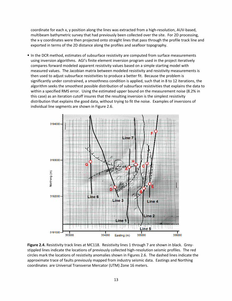
Figure 2.4. Resistivity track lines at MC118. Resistivity lines 1 through 7 are shown in black. Grey-stippled lines indicate the locations of previously collected high-resolution seismic profiles. The red circles mark the locations of resistivity anomalies shown in Figures 2.6. The dashed lines indicate the approximate trace of faults previously mapped from industry seismic data. Eastings and Northing coordinates are Universal Transverse Mercator (UTM) Zone 16 meters.

14

Table 2.1. Measurement statics for DCR Line 1. In each case, the reported values are the average values for the stated channel and electrode configuration defined by the offset between the source electrodes in the gradient array. In each case the nine receiving electrodes used for eight potential measurements were evenly spaced between the source electrodes in the gradient array configuration. SD is the sample standard deviation for the corresponding measurement. The measurements were made while the array was moving through the water in CRP acquisition mode. Hence, the standard deviations reflect the sum of variation to location and noise.

Channel Potential (µV) Potential SD (µV)

Current (mA)

Current SD (mA) Ra (Ωm) Ra SD (Ωm)

220 m source offset 1 334.2 19.4 1008.3 16.5 0.16 0.01 2 564.1 17.3 1008.3 16.5 0.78 0.02 3 176.3 11.0 1008.3 16.5 0.43 0.03 4 128.4 10.4 1008.3 16.5 0.43 0.04 5 119.2 35.9 1008.3 16.5 0.45 0.14 6 128.6 39.1 1008.3 16.5 0.43 0.14 7 181.8 24.4 1008.3 16.5 0.45 0.06 8 322.1 44.3 1008.3 16.5 0.44 0.06 380 m source offset 1 69.2 18.9 1004.4 8.0 0.07 0.02 2 459.9 33.4 1004.4 8.0 1.23 0.09 3 100.3 73.8 1004.4 8.0 0.45 0.33 4 81.9 107.6 1004.4 69.6 0.46 0.60 5 79.4 91.9 999.0 69.4 0.41 0.49 6 123.1 60.6 999.0 69.3 0.44 0.23 7 254.5 56.9 993.6 97.5 0.46 0.11 8 123.0 14.9 998.9 69.2 0.46 0.05

600 m source offset 1 172.8 46.0 997.5 3.2 0.25 0.07 2 221.5 54.4 997.5 3.2 0.91 0.22 3 65.5 41.1 991.9 71.4 0.46 0.30 4 33.3 217.0 991.9 71.4 0.30 1.97 5 72.7 224.6 997.5 3.2 0.66 2.04 6 54.4 100.8 992.0 69.8 0.38 0.71 7 110.0 46.2 986.3 99.5 0.42 0.55 8 303.4 79.1 997.5 3.2 0.45 0.12 800 m source offset 1 253.6 36.0 931.4 67.1 0.53 0.07 2 49.0 76.7 926.0 94.5 0.1 2.85 3 53.1 68.9 926.0 94.4 0.89 4.95 4 38.4 46.8 936.6 2.7 0.49 0.60 5 38.7 60.4 936.6 2.7 0.50 0.78 6 75.3 343.5 936.6 2.7 0.75 3.45 7 4257.1 4405.3 936.6 2.7 24.72 25.56 8 -3800.6 4324.5 936.6 2.7 -7.92 9.01

15

Channel Potential (µV)

Potential SD (µV)

Current (mA)

Current SD (mA) Ra (Ωm) Ra SD (Ωm) Potential (µV) Potential SD

(µV) Current

(mA) Current SD

(mA) Ra (Ωm) Ra SD (Ωm)

1,100 m source offset 1 328.9 79.6 830.7 4.4 1.15 0.28 2 98.2 126.9 830.7 4.4 1.08 1.39 3 -164.7 117.0 826.0 59.3 -2.92 2.09 4 47.0 153.0 816.6 102.1 087 3.75 5 7792.0 1435.4 830.7 4.4 174.08 32.65 6 -1200.7 736.1 826.0 59.4 -22.50 13.65 7 -4927.2 1139.9 826.0 59.4 -47.46 10.59 8 239001.3 18998.1 830.7 4.4 839.06 66.33

16

17

Figure 2.5. Example inverted resistivity sections. a. Segment from Line 1. b. Segment from Line 2. c. Segment from Line 3. d. Segment from Line 4. e. Segment from Line 6. f. Segment from Line 7. Note that the spatial and resistivity scales are different for each section. Red arrows mark resistivity anomalies of note. The locations of the anomalies within the MC 118 study area are shown in Figure 2.5.

2.2.3 Interpretations of DCR profiles. The most surprising result from the reconnaissance DCR survey of MC118 is how little of Woolsey Mound is underlain by high-resistivity material (>100 Ωm), indicative of high-saturation to massive hydrate. Although the line spacing achieved in the survey is sparse (~200 m), it is sufficient to rule out large areas underlain by massive hydrate. This contradicts the pre-survey working model of hydrate distribution at the site (Figure 1.1). Instead, only two small areas were found, both on the scale of a few tens of meters wide and deep, which have resistivities high enough to indicate massive hydrate. These anomalies are labeled “A” and “B” in Figure 2.6 a. and 2.6 b. Both anomalies occur in small pockets, near the seafloor, where previously mapped, deep-seated normal faults intersect the seafloor (Figure 2.5). Furthermore, at places were the same fault scarps where crossed by other resistivity lines, the anomalies are present, but at much lower amplitude. For example, the 10 Ωm anomaly labeled “H”

18

occurs near the south end of Line 7 (Figure 2.6 f.), where it crosses the fault scarp along which the 100 Ωm anomaly “A” occurs, just 200 m to the West (Figure 2.6 a.). Similarly, the 3.2 Ωm anomaly labeled “E” on Line 4 (Figure 2.6 d.) occurs along the same fault scarp on which the 100 Ωm anomaly “B” occurs, just 300 m to the southwest (Figure 2.6 b.). This indicates that the high-resistivity anomalies indicative of massive hydrate are localized not only to the fault traces, but to points along the fault traces as well. In addition to the two high-resistivity anomalies (>100 Ωm ) found in the reconnaissance survey, there are regions of intermediate elevated resistivity in the 3 to 12 Ωm range. Some of these regions of elevated resistivity occur in recognized faults zones such as “E” and “H”, mentioned above, plus “C” on Line 2 (Figure 2.6 b.) and “D” on Line 3 (Figure 2.6 c.). There are also anomalies in this resistivity range that are not associated with previously mapped faults, such as “F” on Line 4 (Figure 2.6 d.) and “G” on Line 6 (Figure 2.6 g.). Resistivities in the 3 to 12 Ωm range have high resistivities relative to an average resistivity of 0.66 Ωm for line segments in the sediments adjacent to the mound, but well below those >100 Ωm that are likely associated with massive hydrate. These intermediate anomalies are likely in part due to the limestone cap (Figure 1.2 b.), in part due to free gas in the sediment and in part due sediment containing lower concentrations of hydrate, such as that found in core samples (Figure 1.2 c. and d.) Like the >100 Ωm anomalies, most of these regions of intermediate resistivity occur within 50 m of the seafloor, but some extend to the limits of penetration of the DCR system near 100 m below bottom. 2.2.4 Evaluation of the validity of DCR inversions. Resistivity data inversion, like all potential-field methods in geophysics suffers from the problem on non-uniqueness, meaning that multiple sub-surface models can explain the same data set. The question is, how does one know that the sub-surface distributions of resistivity shown in Figure 2.6 are not just an artifact of the inversion process and do not reflect actual subsurface conditions? Without direct sampling of the sub-surface, it is not possible to answer this question with 100% certainty. However, there are ways to test for obvious problems. One test is to use a forward resistivity model that predicts the voltages one would measure using the same array patterns and offsets of the actual survey, but computed for a synthetic model that captures the main features of the sub-surface interpretation from the survey data. This was done using the finite element forward modeling feature of AGI’s EarthImager2D (Figure 2.7). The synthetic model consisted of a seawater column with a resistivity of 0.36 Ωm, a background, non-hydrate-bearing sediment resistivity of 2 Ωm, a 200 m thick block of material with a resistivity of 12 Ωm to represent a sediment/hydrate mixture, and a 50 m wide, 100 m thick block of 100 Ωm material to represent massive hydrate within a narrow fault zone. The forward modeled apparent resistivities from the synthetic model were then inverted using the same inversion routine with the same parameters used to produce the inversions shown in Figure 2.6. The resulting inversion of the synthetic model is shown in Figure 2.7 b. The general agreement between the starting synthetic model (Figure 2.7 a.) and the inversion of the forward modeled data does not prove that the inversions shown in Figure 2.6 are the actual sub-surface resistivity distributions. However, it does show that if such distributions do exist, they would produce inversion images from the measurements made similar to those shown in Figure 2.6. Another approach to testing the validity of a potential-field interpretation, short of direct sampling, is to compare the results produced by other, complimentary geophysical methods. Results that show anomalous bodies in the same locations and predicted physical properties that correlate in reasonable ways, lend support to the potential-field interpretation. Prior to the DCR survey conducted in this study, an extensive grid of high-frequency, single channel seismic data was collected over Woolsey Mound . The grid consisted of a set of N-S profiles, spaced 50 m apart and a second set of E-W profiles

19

space approximately 100 m apart (Figure 2.5). The limitation of these data has been that, although stratigraphy and faults in the areas adjacent to the mound are well imaged, the area directly beneath Woolsey Mound is a no record zone. That is, there are no coherent reflections from beneath the mound, only incoherent scatter (Figure 2.8). Prior to the collection of the DCR data, no particular significance was placed on the patterns of seismic scatter. However, when DCR Line 1 was superimposed on the seismic line that most closely followed its path, a distinct pattern emerged. The high-resistivity anomaly, with resistivity greater than 100 Ωm, corresponds to a zone of low scatter surrounded by a zone of high scatter on the seismic profile. The area surrounding the high-resistivity anomaly, with intermediate resistivities in the 3 to 12 Ωm range, corresponds to the surrounding zone of high-scatter. Piston core samples containing churned sediments and angular clasts of massive hydrate were collected from the high-scatter, intermediate resistivity zone, north of the high-resistivity anomaly. This suggests that the churned sediment containing angular hydrate clasts efficiently scatters the high-frequency seismic signal, whereas the high-saturation to massive hydrate does not.

Figure 2.6. Inversion of forward model data. a. Synthetic finite element model of sub-bottom resistivity distribution similar to that indicated by the inversion of data collected along DCR Line 1 (Figure 2.6 a). b. Inverted resistivity section produced from forward modeled apparent resistivity values computed from synthetic model shown in part a.

20

Figure 2.7. Superposition of resistivity and seismic data. Superposition of DCR Line 1 onto a parallel Shallow-Source-Deep-Receiver (SSDR) single channel seismic profile across Woolsey Mound. The seismic profile was one of 83 profiles collected by Tom McGee of University of Mississippi in a N-S, E-W grid over Woolsey Mound (Figure 2.5). The line shown happened to follow the path of DCR Line 1. a. The total energy seismic attribute, shows coherent reflections in areas adjacent to the mound and incoherent scatter from beneath the mound. b. Superposition of DCR Line 1 (Figure 2.6 a.) onto the co-located seismic profile. The horizontal scales where changed to match those of the seismic data. The vertical axis of the resistivity data was converted from depth to two-way travel time, assuming a seismic velocity of 1600 m/s. c. DCR Line 1 scaled to match the SSDR seismic profile.

2.2.5 Discussion of Results of Phase 1 Phase 1 accomplished several of the overall goals of the project. First, it demonstrated that valid DCR data could be collected in nearly 1 km of water. There were reviewers at various stages of the project that expressed doubt that a long electrode array could be towed over the bottom and that even if it could, it would quickly be destroyed by abrasion. There were also reviewers that suggested that even if DCR data could be collected, it would not detect hydrate, because its high resistivity would be masked by an envelope of increased pore-water salinity as a result of the hydrate formation process. However, in the reconnaissance survey the 1.1 km long array was towed for 30 hours over the bottom, while 26 km of data were collected, and the recovered array showed no sign of wear or damage. This proves that seafloor DCR data can be collected in deep water. The data contains two anomalies with resistivities greater than 100 Ωm, which from their location and amplitude strongly suggest the causative bodies are high-saturation to massive hydrate. There were also extensive areas of elevated resistivity in the 3 to 12 Ωm range. Piston core samples from one of these areas shows low concentrations (5 to 10%) of hydrate present in the form of clasts of massive hydrate (Figure 1.2 c and d.). A presentation of these results was made at the 2010 Symposium on the Application of Geophysics to Engineering and Environmental Problems, held in Keystone, Co., April 11-15, 2010 (Dunbar et al., 2010).

The second objective of Phase 1 was to determine the overall distribution of hydrate beneath Woolsey Mound, MC118. The results of the reconnaissance survey clearly show that the working model of hydrate distribution circa 2005 is incorrect (Figure 1.1). There appear to be only small zones of high-saturation hydrate, rather than large areas underlain by massive hydrate as proposed. It shows that the high-saturation hydrate occurs within fault zones, but not pervasively within fault zones. There also

21

appears to be more extensive zones surrounding the faults that contain low concentrations of massive hydrate. Based on these results, a new model for the formation and movement of hydrate at MC118 was formulated. The concept is that the massive hydrate blocks seen on the seafloor initially form in the sub-surface within fault zones, as free methane seeps up from deep reservoirs and into the HSZ. Once a sufficient accumulation of hydrate occurs locally on the fault, it moves upward along the fault, driven by buoyancy forces associated with the relative low density of hydrate compared to the surrounding sediment. As the hydrate blocks move, they break apart, and some of the hydrate becomes mixed with the deformed sediment within the fault zone. Finally, the carbonate cap is broken and blocks of carbonate are shoved aside, as the hydrate is extruded out onto the seafloor. The mechanical feasibility of this mode of hydrate emplacement was tested using a finite element geodynamics model and reported in a conference proceedings (Dunbar, 2011).

In one aspect, the original goals for Phase 1 were not completely met by the reconnaissance survey. The main limitation of the survey was that the lines were spaced too far apart, given the small size of the high-saturation hydrate bodies. The survey was designed based on the working model of hydrate distribution, which suggested that the mound was underlain by significant areas of high-saturation hydrate. The primary question was at what depth these bodies occur. In that case, a coarse spacing of a few 2D lines would have been sufficient to characterize the distribution of hydrate at the site. However, given that the high-saturation hydrate bodies appear to be only a few tens of meters across, it was likely a matter of luck that we found any at all. Imaging these small anomalous bodies clearly would require a high resolution 3D resistivity survey with much smaller line spacing (~50 m) and full 3D processing. For this reason, at the completion of Phase 1, it was proposed that too little was known about the distribution of hydrate at the site to justify reconfigure the DCR system for long term monitoring of one of the two anomalies found. Instead, the proposal was made and accepted, to reconfigure the DRC system for 3D acquisition and to devote Phase 2 to making a more complete assessment of the distribution of hydrate beneath Woolsey Mound.

3 Phase 2: Reconfiguring the DCR System and 3D Survey (Task 2.1)

3.1 Reconfiguration of the DCR system for 3D acquisition The main limitations of the reconnaissance survey conducted in Phase 1 of the project were that the array used was designed for fixed recording in which the source and receiver electrodes were interchangeable and made of graphite to prevent corrosion over long deployments. The signal to noise level in the CRP survey using this array was relatively poor. The results of the Phase 1 survey indicated that the most interesting resistivity anomalies, suggestive of high concentration hydrate deposits, occur within 50 m of the seafloor. Hence, the goals of the DCR system reconfiguration for Phase 2 were to improve near-bottom resolution and to increase the signal to noise ratio of the DCR measurements. The three main changes were made to the DCR system from the reconnaissance 2D survey configuration. First, a new shorter electrode array was built, with dedicated source and receiver electrodes. That is, unlike in the general-purpose reconnaissance survey array, the source and receiver assignments were fixed throughout the survey. This made it possible to use larger and more efficient copper electrodes connected by heaver-gauge wire for the sources and low-noise titanium electrodes for the receivers (Figure 3.1). The completed array has electrical connections for two replaceable, copper source electrodes spaced 50 m apart at the lead end and one at the trailing end of the array. There are ten titanium receiver electrodes spaced 50 m apart along the array, starting at the second source electrode

22

and ending at the trailing source electrode. This configuration makes two array configurations possible. Using the first and last source electrodes and receiver electrodes 1 through 9, produces a 500 m long gradient array, with A and B source electrodes at the ends and receiver electrodes spaced 50 m apart between. The gradient array is a generalized form of the Wenner array, which provides maximum depth of penetration and signal level for a given array length. This was the configuration that was used in the reconnaissance survey for Phase 1 of the project. Using the first two source electrodes and receiver electrodes 2 through 10, produces a 500 m long dipole-dipole array, with the source dipole at the front of the array and 8 receiver dipoles spaced along the array. This configuration offers higher depth resolution at the expense of depth of penetration and signal level.

Figure 3.1. Titanium receiver electrode. The new resistivity array for Phase 2 has 10 dedicated receiver electrodes made of titanium and three dedicated source electrodes made of copper. The electrodes were molded into the array at fixed positions, 50 m apart. The electrode shown is a 20 cm-long, titanium receiver electrode, molded into place on the cable.

The second change to the DCR system was an external, low-noise preamplifier that was added to the front end of the cable to boost the signal level by a factor of 100. Electrical noise in the deep marine environment is low at frequencies higher than 1 Hertz, because high-frequency electromagnetic noise in the atmosphere is attenuated by the thick seawater layer. The idea was to boost the signal level in an external preamplifier before the signal enters the main housing, where the onboard computer generates radio-frequency noise. Together, the improved electrodes and the preamplifier should dramatically increase the signal-to-noise ratio and shallow resolution over that achieved in the reconnaissance survey.

The third change to the DCR system, was to add four three-component digital-recording fluxgate magnetometers to the electrode array. The magnetometers, each in its own miniature pressure housing, have brackets that allow them to be attached to the electrode array at intervals to record the bearing and tilt of the array during acquisition. From these measurements it is possible to work backwards from

23

the tow body to estimate the geographic location of the electrodes. This would eliminate reliance on the assumption that the array follows the path of the tow body.

3.2 Attempted 3D DCR survey of MC118 With these changes, the reconfigured system was completed in March, 2011 and tested in a water reservoir at full scale. The system was then crated, ready for deployment in the second leg of a June 2011 to MC118. However, during the first leg of the cruise, the SSD ROV was damaged to the point it was inoperable. Hence, the second leg, which included the planned 3D DCR survey, was canceled. A second no-cost extension to the project was applied for and received and the DCR system was mothballed for a year, while the SSD ROV was repaired. During the summer of 2012 preparations were made to process the DCR 3D data that was to be acquired in a July, 2012 cruise of MC118. Graduate student Tian Xu, tested 3D binning algorithms for converting irregularly spaced CRP profiling data into binned readings on regular grids, in preparation for 3D inversion. Xu reported the results of this binning procedure at the 2013 Symposium on the Application of Geophysics to Engineering and Environmental Problems, held in Denver CO., March 17-21, 2013 (Xu and Dunbar, 2013). The SSD ROV was repaired and ready to go just prior to a July, 2012 cruise to MC118. The DCR system was deployed in the evening of the last day of the cruise. However, no resistivity data were collected. The resistivity system was operational while on deck, but communication with the instrument was lost on the way to the bottom. Upon retrieval, it was found that the main instrument housing had flooded. The failure was due to a slipped O-ring. Subsequent efforts to recover the system components were not successful, meaning that a new set of system cards will be required to make the instrument operational. It appears that during the sealing of the instrument house, one of the two O-rings on the housing end cap slipped out of place and was caught in the part of the end cap that fits into the housing. The displaced O-ring thereby interfered with the seal of the second O-ring. Insufficient funds remained in the project budget to replace the DCR system cards. Hence, the project was terminated without completion of Phase 2.

3.3 Discussion of Phase 2 failure In the section assessing risk factors to the success of the project in the original proposal, the main risks recognized were the normal risks faced by all projects that involve putting instrumentation on the deep seafloor. These included damage to instrumentation due to the harsh environment of the deep seafloor. This project was originally planned as a three year, but ended up spanning six years. Three major setbacks occurred during the project. The first electrode array was destroyed by sharks, minutes after it was placed in the water for the first time. This cost the project one year of lost time and 16% of the total budget. The SSD ROV needed to support the DCR system was heavily damaged in unrelated activities, resulting in a second year of lost time. Then after a year of work modifying the system for 3D acquisition, the instrument was lost because of a slipped O-ring. In spite of this setback, the two main goals of the project had been achieved. A prototype DCR system was developed and successfully used to locate resistivity anomalies likely associated with high-saturation to massive hydrate at MC118. This project demonstrated that the DCR method works in the deep marine environment and can be used to image resistivity variations in the upper 100 m on the scale of 10 m or less, in settings that are no-record areas for high-frequency reflection seismic data. This is approximately a factor of 10 better spatial resolution than has been achieved with existing CSEM systems. Furthermore, much of the development work need to conduct 3D DCR surveys was completed, even though it was not implemented.

24

References Constable, S. and C. S. Cox, 1996, Marine controlled source electromagnetic sounding: 2. The PEGASUS

experiment, Journal of Geophysical Research, v. 101, 5519-5530. Cox, C. S., S. C. Constable, A. D. Chave, and S. C. Webb, 1986, Controlled source electromagnetic

sounding of the oceanic lithosphere, Nature, v. 320, p. 52-54. Dunbar, J. A., 2012, Extrusion model for the distribution of hydrate at Woolsey Mound, Mississippi

Canyon, Block 118, Gulf of Mexico, 2012 Ocean Sciences Conference, Book of Abstracts, page 119, Salt Lake City, Utah, February 20-24, 2012.

Dunbar, J., A. Gunnell, P. Higley, M. Lagmanson, 2010, Seafloor resistivity investigation of methane hydrate distribution in Mississippi Canyon, Block 118, Gulf of Mexico, (expanded abstract) Symposium on the Application of Geophysics to Engineering and Environmental Problems, v. 23, p. 835-844.

Weitemeyer, K.A., Constable, S.C., Key, K.W., Behrens, J.P. [2006] First results from a marine controlled – source electromagnetic survey to detect gas hydrates offshore Oregon. Geophysical Research Letters 33, L03304.

Xu, T. and J. Dunbar, 2013, Binning method for mapping irregularly distributed continuous resistivity profiling data onto a regular grid for 3D inversion, (expanded abstract) Symposium on the Application of Geophysics to Engineering and Environmental Problems, Denver CO., March 17-21, 2013.