Electric Powertrains: Opportunities and Challenges in the U.S. Light-Duty Vehicle Fleet

Matthew A. Kromer and John B. Heywood

May 2007 LFEE 2007-03 RP

Sloan Automotive Laboratory

Laboratory for Energy and the Environment Massachusetts Institute of Technology

77 Massachusetts Avenue, Cambridge, MA 02139

Publication No. LFEE 2007-03 RP

- 2 -

- 3 -

Abstract Managing impending environmental and energy challenges in the transport sector requires a dramatic reduction in both the petroleum consumption and greenhouse gas (GHG) emissions of in-use vehicles. This study quantifies the potential of electric and hybrid-electric powertrains, such as gasoline hybrid-electric vehicles (HEVs), plug-in hybrid vehicles (PHEVs), fuel-cell vehicles (FCVs), and battery-electric vehicles (BEVs), to offer such reductions. The evolution of key enabling technologies was evaluated over a 30 year time horizon. These results were integrated with software simulations to model vehicle performance and tank-to-wheel energy consumption; the technology evaluation was also used to estimate costs. Well-to-wheel energy and GHG emissions of future vehicle technologies were estimated by integrating the vehicle technology evaluation with assessments of different fuel pathways. While electric powertrains can reduce or eliminate the transport sector’s reliance on petroleum, their GHG and energy reduction potential are constrained by continued reliance on fossil-fuels for producing electricity and hydrogen. In addition, constraints on growth of new vehicle technologies and slow rates of fleet turnover imply that these technologies take decades to effect meaningful change. As such, they do not offer a silver bullet: new technologies must be deployed in combination with other aggressive measures such as improved conventional technology, development of low-carbon fuels and fuel production pathways, and demand-side reductions. The results do not suggest a clear winner amongst the technologies evaluated, although the hybrid vehicle is most likely to offer a dominant path through the first half of the century, based on its position as an established technology, a projection that shows continued improvement and narrowing cost relative to conventional technologies, and similar GHG reduction benefits to other technologies as long as they rely on traditional fuel pathways. The plug-in hybrid, while more costly than hybrid vehicles, offers greater opportunity to reduce GHG emissions and petroleum use, and faces lower technical risk and fewer infrastructure hurdles than fuel-cell or battery-electric vehicles. Fuel-cell vehicle technology has shown significant improvement in the last several years, but questions remain as to its technical feasibility and the relative benefit of hydrogen as a transportation fuel.

This research was funded by Ford Motor Company through the Alliance for Global Sustainability (AGS), CONCAWE, ENI, Shell, and Environmental Defense.

- 4 -

- 5 -

Table of Contents Table of Contents............................................................................................................................ 5 List of Figures ................................................................................................................................. 7 List of Tables ................................................................................................................................ 10 Abbreviations................................................................................................................................ 13 1 Introduction........................................................................................................................... 15

1.1 Greenhouse Gas Emissions and Petroleum Use in Transportation............................... 15 1.2 Research Overview and Motivation.............................................................................. 16 1.3 Context.......................................................................................................................... 18 1.4 Overview of the Study .................................................................................................. 23

2 Methodology......................................................................................................................... 24 2.1 Overview....................................................................................................................... 24 2.2 Simulation Methodology .............................................................................................. 24 2.3 Previous Work .............................................................................................................. 25 2.4 Assumed Vehicle Characteristics ................................................................................. 26 2.5 Cost Methodology......................................................................................................... 27 2.6 Well-to-Tank Energy Use and GHG Emissions ........................................................... 28 2.7 Embodied Vehicle Energy: Cradle-to-Grave Energy Use ............................................ 28

3 Battery Technology: Current Status & Future Outlook........................................................ 30 3.1 Introduction................................................................................................................... 30 3.2 Energy Storage Requirements....................................................................................... 30 3.3 Battery Technology: Current Status.............................................................................. 34 3.4 Battery Technology: Future Trends .............................................................................. 37 3.5 Summary: Battery Assumptions ................................................................................... 46

4 Spark-Ignition Engines, Diesels, and Hybrids ...................................................................... 48 4.1 Key Assumptions about the Hybrid Vehicle ................................................................ 48 4.2 Adjustments to the Hybrid Vehicle Model ................................................................... 49 4.3 Special Considerations.................................................................................................. 50 4.4 Cost Projections for NA-SI, Turbo, Diesel, and Hybrid Vehicles................................ 56 4.5 Summary....................................................................................................................... 57

5 Plug-In Hybrid-Electric Vehicles ......................................................................................... 58 5.1 Overview....................................................................................................................... 58 5.2 Plug-in Hybrid Defined................................................................................................. 58 5.3 Methodology................................................................................................................. 59 5.4 Vehicle Design Constraints........................................................................................... 59 5.5 Plug-In Hybrid Vehicle Configurations........................................................................ 62 5.6 Incremental Cost of the Plug-In Hybrid........................................................................ 72 5.7 Electricity Fuel Cycle ................................................................................................... 74 5.8 GHG Emissions ............................................................................................................ 81 5.9 Implementation Questions ............................................................................................ 82 5.10 Conclusion .................................................................................................................... 85

6 Electric Vehicles ................................................................................................................... 87 6.1 Introduction................................................................................................................... 87 6.2 Vehicle Configuration................................................................................................... 87 6.3 Sizing the Battery Pack................................................................................................. 87 6.4 Sensitivity to Assumptions ........................................................................................... 89

- 6 -

6.5 Conclusion .................................................................................................................... 90 7 Fuel-Cell Vehicles ................................................................................................................ 91

7.1 Vehicle .......................................................................................................................... 92 7.2 Hydrogen Storage ....................................................................................................... 106 7.3 Vehicle Simulation...................................................................................................... 107 7.4 Fuel Cycle ................................................................................................................... 110 7.5 WTW Results.............................................................................................................. 112 7.6 Conclusion .................................................................................................................. 112

8 Results................................................................................................................................. 114 8.1 Well-to-Wheel Energy, Petroleum, and GHG Emissions........................................... 116 8.2 Costs & Cost-Effectiveness ........................................................................................ 117 8.3 Discussion ................................................................................................................... 119

9 Conclusions......................................................................................................................... 134 10 Recommendations........................................................................................................... 136 References................................................................................................................................... 137 Appendix 1: Base Case Vehicle Configurations......................................................................... 144 Appendix 2: Fuel Consumption & Energy Use .......................................................................... 145 Appendix 3: Battery Assumptions .............................................................................................. 146 Appendix 4: Fuel-Cell System Model Assumptions .................................................................. 148

Base Case Fuel Cell System Operating Map .......................................................................... 149 Conservative Fuel Cell System Operating Map...................................................................... 150

Appendix 5: Plug-In Hybrid Configuration, Calculations, and Results ..................................... 151 Appendix 6: Hybrid Vehicle Configurations & Results of Accessory-Load Tests .................... 152 Appendix 7: Definition of Vehicle Technologies ....................................................................... 153

- 7 -

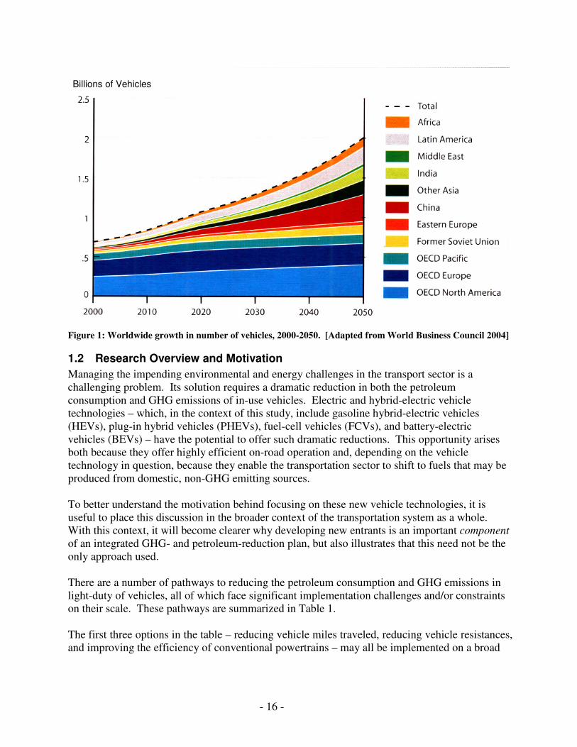
List of Figures Figure 1: Worldwide growth in number of vehicles, 2000-2050. [Adapted from World Business

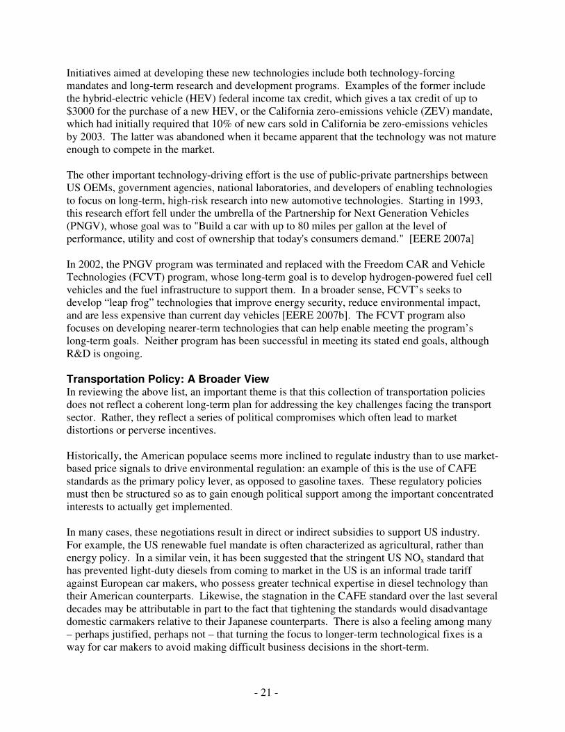
Council 2004]........................................................................................................................ 16 Figure 2: Trends in the US Auto-Market, 1975-2005. Source: EPA 2006a ................................ 19 Figure 3: Improvements in lithium-ion battery technology, 1991-2001 [Adapted from Brodd

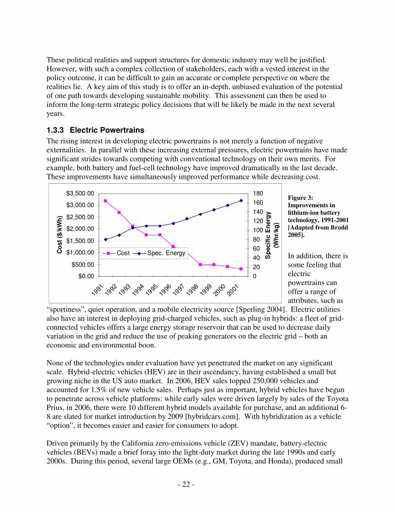
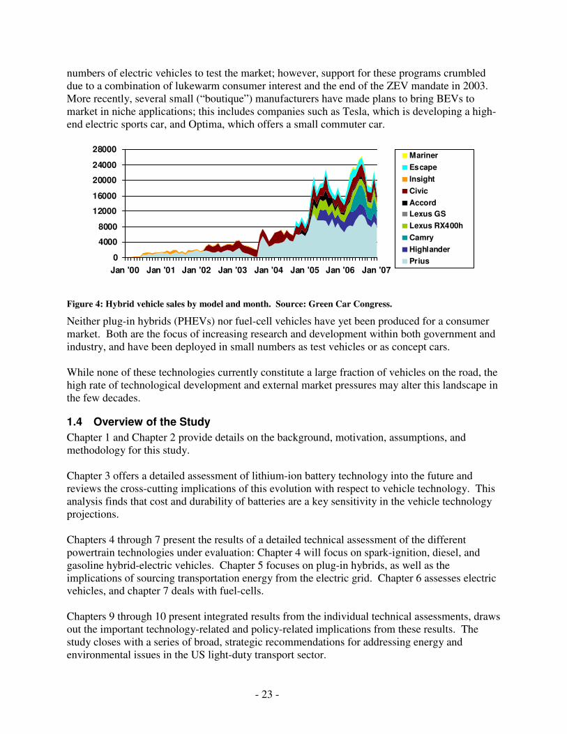
2005]. .................................................................................................................................... 22 Figure 4: Hybrid vehicle sales by model and month. Source: Green Car Congress.................... 23 Figure 5: ADVISOR Simulink block diagram.............................................................................. 25 Figure 6: Change in total lifecycle GHG emissions/energy use relative to the NA-SI due to the

embodied energy. .................................................................................................................. 29 Figure 7: Illustration of a typical Plug-In Hybrid duty cycle........................................................ 31 Figure 8: Histogram of the C-Rate for charge-sustaining operation in the hybrid and plug-in

hybrid vehicle (30-mile range) over the US06 drive cycle. Note that the plug-in hybrid power requirement rarely goes above 2.5C (the histogram clusters around 0), while the HEV requirements dictate operation well in excess of 5C. Operation over the US06 cycle corresponds to a high-end ESS requirement. ........................................................................ 33

Figure 9: Ragone plot of different energy storage options. Source: [Srinivasan 2004]....... 34 Figure 10: Historical change in lithium-ion battery specific-energy since its introduction in 1991.

(~7%/year). It should be noted that improving specific energy for consumer electronic applications formed the primary focus of development over this timeframe. Source: Brodd 2005....................................................................................................................................... 35

Figure 11: Comparative economies of scale for Lithium-ion (Li-Ion) and Nickel-Metal Hydride (NiMH) batteries. Based on internal studies at Ford. Source: Miller, 2006 ...................... 36

Figure 12: Effect of calendar life and temperature on storage capacity (LiFePO4 cathode) [Adapted from Chu 2006]..................................................................................................... 39

Figure 13: Specific power and energy of present-day and projected future lithium-ion battery modules. (Present day data: The high-energy li-ion battery is the Saft VLE Li[Co.2Ni.8]O2 chemistry; low-energy battery is A123 ANR26650, using a LiFePO4 chemistry). Module is estimated to weigh 25% more than the cell. Source: A123, Saft......................................... 42

Figure 14: Projected cost breakdown for high-energy lithium-ion battery modules at high volume production and with incremental material cost reduction..................................................... 43

Figure 15: Current and future battery cost as a function of battery rate capability. Current data is based on a review of industry data and private correspondence [Miller 2007, Anderman 2000, Anderman 2005]. ........................................................................................................ 45

Figure 16: Energy flows over the different drive cycles (Left: HEV; Right: 2030 NA-SI) ......... 51 Figure 17: Fuel consumption benefit as a function of drive cycle for different vehicle

technologies. ......................................................................................................................... 52 Figure 18: Air-conditioning energy use in conventional and hybrid vehicles. The “Extra Fuel”

bar (far left) is the amount of extra energy (in terms of gasoline use) that is required to run the air conditioning over different drive cycles. The two right-most bars (“Engine Braking” and “Improved [Engine] Efficiency”) represent the portion of air conditioning energy that is met by improving vehicle efficiency. The z-axis is normalized to a distance of 11 miles (the length of the FTP drive cycle). ............................................................................................. 53

Figure 19: Estimated thermal loads for a present-day passenger car under different environmental conditions as a function of recirculated air. Adapted from [Farrington 2000]. ................... 54

Figure 20: Impact of air conditioning loads on hybrid vehicle fuel consumption........................ 55

- 8 -

Figure 21: PHEV operating modes. .............................................................................................. 58 Figure 22: Sample utility curve for the data set in Table 18......................................................... 60 Figure 23: Estimated utility curves as a function of vehicle range: estimates from a number of

different sources. Data derived from SAE J1711, EPRI 2001, Markel 2006, and ORNL 2004....................................................................................................................................... 61

Figure 24: Qualitative representation of the PHEV design space................................................. 62 Figure 25: Fuel flow rates for the ICE during the US06 drive cycle: the top figure shows an

engine that does not need to warm up; the bottom requires that the engine reach 96 F. The vehicle with no engine warm-up (upper plot) shows engine operation as a series of 12 discrete spikes – in addition to drivability questions, this represents many additional cold starts. When this is compared against lower plot, which does require a warm-up period, there are several instances in which the engine is forced to remain on for an extended period (see, e.g., from ~50-200 seconds). ........................................................................................ 64

Figure 26: Tank-to-wheels petroleum consumption as a function of drive cycle and hybridization ratio. The data is aggregated over charge-depleting and charge-sustaining mode. FTP, HWFET, and Combined data are adjusted (0.9/0.78) numbers. The 55% vehicle runs all-electric; the other vehicles run in blended mode. ................................................................. 66

Figure 27: Petroleum consumption, relative to the all-electric (55%) hybridized configuration for the three vehicles using blended mode (hybridization ratios of 44%, 36%, and 26%). ....... 66

Figure 28: Petroleum consumption as a function of distance between recharge and hybridization ratio. ...................................................................................................................................... 68

Figure 29: Tank-to-wheels energy use as a function of drive cycle and hybridization ratio. The data is aggregated over charge-depleting and charge-sustaining mode. FTP, HWFET, and combined data are adjusted (0.9/0.78) numbers. The 55% vehicle runs all-electric; the other vehicles run in blended mode. .............................................................................................. 69

Figure 30: Breakdown of Tank-to-Wheel (TTW) Energy Use in the US06 Cycle ...................... 69 Figure 31: Aggregate energy and petroleum use as a function of electric range over the combined

adjusted FTP/HWFET drive cycle. The conventional (“0-mile”) hybrid vehicle is included for reference. ......................................................................................................................... 71

Figure 32: Evolution of US Average Grid Mix, 2005-2030. Source: EIA 2006......................... 76 Figure 33: Projected US electricity generation by source, 2005-2030. Source: EIA 2006 ......... 76 Figure 34: Illustrative example of electric grid dispatch. Source: Keith 2004 ............................ 78 Figure 35: Typical load-shape and generation sources. Adapted from [Kintner-Meyer 2006]... 78 Figure 36: Predicted share of natural gas vs coal on the margin using the capacity factor method.

Intermediate generation defined as 30%<capacity factor<60%. Source: EPA 2002........... 79 Figure 37: Emissions rate from the electric grid for different generation sources. The first

number represents the emissions from generating 1 MWh of electricity; the second number represents the emissions from delivering 1 MWh of electricity to the vehicle. The “clean grid” corresponds to a grid composed of 50% non-GHG emitting sources, 15% combined-cycle natural gas generation, and 35% coal. ......................................................................... 81

Figure 38: Breakdown of GHG emissions for the hybrid vehicle and plug-in hybrids with varying range. The low-end of the uncertainty bar corresponds to natural gas generation; the high-end corresponds to coal; and the base case corresponds to the average grid. The arrows indicate the emissions rate of the clean grid mix identified in section 5.7.4. ....................... 82

Figure 39: Sensitivity of range to energy used. ............................................................................ 88 Figure 40: Cost of increasing electric range ................................................................................. 89

- 9 -

Figure 41: A series-hybrid fuel-cell vehicle architecture. Arrows show possible power flows: The fuel-cell converts hydrogen to electricity, which is used to either deliver traction power to the motor or to charge the battery; a portion of the vehicle’s kinetic energy may be recovered through regenerative braking. .............................................................................. 92

Figure 42: Historical evolution of fuel-cell stack power density. Source: Carlson 2005 ............. 94 Figure 43: Illustration of fuel-cell stack losses [Frost 2006] ........................................................ 94 Figure 44: Evolution of fuel-cell polarization curves. Historical data from [Guzy 2006]. ......... 95 Figure 45: Fuel-cell System, from [Ahluwalia 2005]................................................................... 96 Figure 46: Fuel-cell stack and system efficiency for the baseline case. Assumes the balance-of-

plant includes an integrated compressor-expander module, and that the system rated power occurs at 0.65 V and 1500 mA/cm2. ..................................................................................... 98

Figure 47: Fuel-cell stack and system efficiency for the conservative case. Assumes the balance-of-plant does not include an expander module, and that the system rated power occurs at 0.60 V and 1500 mA/cm2...................................................................................................... 99

Figure 48: Historical progression of high-volume fuel-cell stack cost projections from different sources. The short-term 2010 DOE target ($30/kW) is shown for reference. Data from: [Ballard 2007, NRC 2005, and Carlson 2005].................................................................... 100

Figure 49: Breakdown of fuel-cell system costs at high-volume production using 2005 technology. Assumes a stack power density of 600 mW/cm2 and a platinum loading of 0.75 mg/cm2 [Carlson 2005]. ...................................................................................................... 101

Figure 50: Stack cost as a function of platinum loading and power density. Platinum is assumed to cost $900/Oz. .................................................................................................................. 102

Figure 51: Breakdown of balance-of-plant costs. Source: Carlson 2005 .................................. 103 Figure 52: Energy use for the fuel-cell vehicle for different drive cycles. The baseline vehicle

uses a 40% hybridization ratio; the error bar shows the sensitivity to hybridization. The high-end energy use represents 25% hybridization ratio; low-end is 60% hybridization ratio.............................................................................................................................................. 108

Figure 53: Well-to-wheel GHG emissions for different vehicle technologies. .......................... 116 Figure 54: Well-to-wheel energy use for different vehicle technologies. .................................. 116 Figure 55: Relative Energy, Petroleum (in Gasoline Equivalent), and GHG Emissions of vehicle

options, compared to a 2030 NA-SI ................................................................................... 119 Figure 56: Petroleum consumption and GHG emissions for different vehicle technologies and

electricity sources................................................................................................................ 120 Figure 57: Projected domestic and imported petroleum consumption, 2005-2050 [EIA 2006]. 127 Figure 58: Several different vehicle technology penetration scenarios, as well as the business-as-

usual reference case and the targeted reductions. ............................................................... 129 Figure 59: Petroleum reduction scenarios using advanced technology vehicles. ....................... 129 Figure 60: Market penetration rates of different vehicle technologies. Source: Automatic

transmission penetration data from EPA [2006a]; Diesel penetration data from ACEA [2007].................................................................................................................................. 131

Figure 61: Illustrative Integrated GHG-reduction scenarios ...................................................... 133 Figure 62: Illustrative integrated petroleum reduction scenarios ............................................... 133 Figure 63: Saft VLE Discharge curve. Source: [Barsacq 2005] ................................................ 146 Figure 64: Battery equivalent circuit .......................................................................................... 146

- 10 -

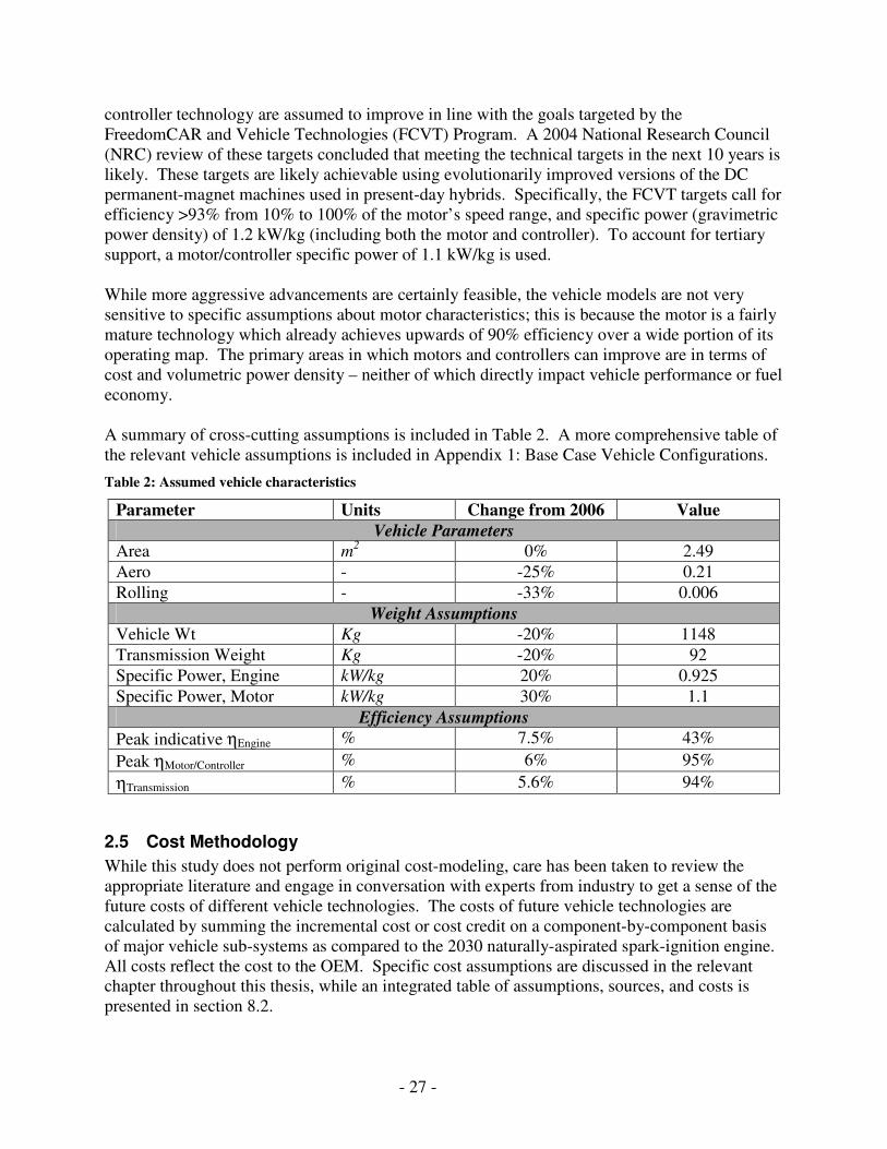
List of Tables Table 1: Pathways to sustainable mobility.................................................................................... 17 Table 2: Assumed vehicle characteristics ..................................................................................... 27 Table 3: Assumed energy and carbon content of different fuel sources. Data is expressed in

terms of the amount of energy or CO2 equivalent released to deliver 1 MJ of fuel to the tank................................................................................................................................................ 28

Table 4: USABC Targets for hybrid-electric and battery-electric vehicle energy storage. [Source: NRC 2005] ............................................................................................................. 30

Table 5: Drivers for ESS requirements for different electric powertrains.................................... 31 Table 6: PHEV cycle-life requirements for charge-sustaining (CS) and charge-depleting (CD)

operation ............................................................................................................................... 32 Table 7: Estimated plug-in hybrid requirements .......................................................................... 33 Table 8: Near-term alternatives to LiCoO2 cathodes. [Buchmann 2006, Ritchie 2004, Ritchie

2006] ..................................................................................................................................... 37 Table 9: Long-Term Lithium-ion Challenges and Mitigation Strategies ..................................... 38 Table 10: Approximate weight battery pack for different electric ranges. Assumes that one

additional kg of battery mass requires 0.5 kg of tertiary vehicle support. The baseline NA-SI weighs approximately 1260 kg......................................................................................... 41

Table 11: Lithium-Ion BEV cost projections (“Cost” = OEM cost from battery manufacturer). 43 Table 12: Assumed ESS characteristics for electric powertrains ................................................. 46 Table 13: Assessment of risk in meeting automotive battery requirements ................................. 47 Table 14: Fuel Consumption Results from [Kasseris 2006] for the 2.5L Camry ......................... 48 Table 15: Changes to the hybrid vehicle since the last study. ...................................................... 49 Table 16: Estimated current and future hybrid vehicle incremental costs. For assumptions about

the future hybrid vehicle cost, see Table 51 and Table 52.................................................... 56 Table 17: Incremental costs, compared to the 2030 NA-SI vehicle, of mainstream technologies.

............................................................................................................................................... 57 Table 18: Sample breakdown of mileage for a PHEV with a 30 mile range................................ 60 Table 19: Vehicle Configurations for Parametric Study; battery energy is 8.2 kWh. .................. 64 Table 20: Acceleration performance as a function of hybridization ratio. ................................... 65 Table 21: Petroleum use, in L/100 km, in the US06 cycle, in charge-depeleting (CD) and charge-

sustaining (CS) mode. The third column shows the vehicle’s range in charge-depleting mode...................................................................................................................................... 67

Table 22: Summary Results for different vehicle options. Energy and fuel consumption are both recorded in terms of L/100 km gasoline equivalent. Combined drive cycle is calculated using adjusted values (0.9/0.78)............................................................................................ 70

Table 23: Comparative petroleum reduction benefits of different PHEV configurations over the combined adjusted FTP/HWFET drive cycle. Reduction is defined (in the case of the NA-SI comparison) as “(FCPHEV – FCNA-SI)/FCNA-SI. .................................................................. 70

Table 24: PHEV battery cycle life requirements. See Chapter 3 for further discussion. ........... 71 Table 25: Battery characteristics for vehicles with different electric ranges................................ 72 Table 26: Estimated OEM battery cost for varying electrical range. ........................................... 72 Table 27: Estimated incremental costs for plug-in hybrid configurations. Data in parentheses

indicates the results for an optimistic cost projection based on a $200/kWh electric-vehicle battery. A comprehensive list of assumptions is detailed in Table 51................................. 72

- 11 -

Table 28: Comparative cost-effectiveness of different PHEV configurations, as compared to the HEV and NA-SI. Results are based on a vehicle lifetime of 150,000 miles. Parentheses indicate the incremental cost for the optimistic cost projection. A comprehensive list of assumptions is detailed in Table 51. ..................................................................................... 73

Table 29: Critical assumptions about characteristics of the electric grid ..................................... 74 Table 30: Current and future US average grid mix. (Source: EIA 2006) .................................... 75 Table 31: Trends in the utility sector and their impact on the base-case projections ................... 77 Table 32: Fuel cycle energy and GHG-emissions for different electricity generation sources. ... 80 Table 33: National PHEV grid charging capacity. Adapted from [Kintner-Meyer 2006]. ......... 83 Table 34: Annual fuel costs for different vehicle options. Assumes: 1.) 15,000 miles/Yr; 2.) Gas

@ $3.00/gal; 3.) Electricity @ $0.05/kWh ........................................................................... 85 Table 35: Vehicle characteristics of electric vehicles with varying electric range. The

calculations assume a 150 Wh/kg battery that costs $250/kWh. .......................................... 88 Table 36: Sensitivity of the 200-mile electric vehicle to the assumed battery characteristics ..... 90 Table 37: 2004 fuel cell status and DOE targets. Source: [NRC 2005] ...................................... 93 Table 38: Fuel-cell Assumptions .................................................................................................. 97 Table 39: Projected high-volume cost and associated projections for several different scenarios.

The assumptions used to meet the DOE target represent a plausible path that could allow industry to meet the cost targets. All four scenarios assume that the cost of platinum is $900/tr oz. ........................................................................................................................... 104

Table 40: Characteristics of different 2004 hydrogen storage technologies. Source: NRC 2005............................................................................................................................................. 106

Table 41: Characteristics of different 2004 hydrogen storage technologies. Source:NRC ....... 107 Table 42: Fuel-Cell Vehicle ADVISOR Model Configuration. DOH = Degree-of-Hybridization

............................................................................................................................................. 107 Table 43: Vehicle Control Parameters ........................................................................................ 108 Table 44: Results for the baseline FCV with 40% degree-of-hybridization. FTP, Hwy, and

Combined energy use is adjusted........................................................................................ 108 Table 45: Vehicle range for varying size and pressure hydrogen storage tanks. The low-end of

the range represents the conservative, 25% DOH vehicle; the high-end corresponds to the baseline 60% DOH. ............................................................................................................ 109

Table 46: Estimated FCV OEM incremental costs compared to the 2030 baseline NA-SI vehicle; assumes 40% hybridization ratio. ....................................................................................... 110

Table 47: Well-to-tank energy use and GHG emissions for different hydrogen production pathways. Source: GREET; an additional 5% energy and CO2 was added to the GREET data to account for the extra energy required to compress from 350 Bar to 700 Bar. (SMR = Steam Methane Reforming)................................................................................................ 111

Table 48: Well-To-Wheel Energy use, Petroleum use, and GHG emissions for the future 2030 FCV. Based on the baseline projections using a 40% hybridization ratio for a vehicle following the combined, adjusted HWFET/FTP drive cycle. Assumes hydrogen is derived from SMR at distributed locations...................................................................................... 112

Table 49: Development path for commercializing fuel-cell vehicles ......................................... 112 Table 50: Energy use, petroleum use, and GHG emissions for all vehicle technologies over the

combined, adjusted HWFET/FTP drive cycle. ................................................................... 115

- 12 -

Table 51: Vehicle component cost assumptions. All costs reflect OEM costs, not retail prices. In general, cost data reflects an overall “sense of the industry”, rather than the results from a single source........................................................................................................................ 117

Table 52: Battery specific cost assumptions; optimistic projection is shown in parentheses..... 117 Table 53: Estimated Incremental OEM Costs for vehicle technologies compared to the 2030 NA-

SI. The impact of optimistic battery projections (based on $150/kWh for a high-energy battery) and conservative fuel-cell projections (based on $75/kW) are reflected in parentheses. Underlying assumptions are summarized in Table 51 and Table 52. ........... 118

Table 54: Costs-Effectiveness and fuel savings, relative to the 2030 NA-SI vehicle. Italics indicate optimistic battery projection/conservative fuel-cell projection. ........................... 118

Table 55: Fuel-cycle GHG-reduction opportunities beyond the base-case projections ............. 121 Table 56: Summary of the outlook for reducing GHG emissions through additional use of low

carbon fuels. The two right-most columns offer a qualitative judgment of 1.) How difficult it is to implement change at large scale; and 2.) The technical risk involved in developing clean production pathways. Lighter shading implies a lesser challenge........................... 123

Table 57: Technological challenges to deployment at scale for advanced electric powertrains. Lighter colored boxes indicate lower technical risk. .......................................................... 123

Table 58: Relative GHG emissions and petroleum consumption of 2030 vehicles compared to the 2006 baseline. ..................................................................................................................... 128

Table 59: Market introduction and early-stage market penetration assumptions ....................... 130 Table 60: Annual rate of sales growth required to go from 5% of new vehicle sales in the

“Starting Year” to the “Target Market Penetration” in the year 2040 (which allows us to meet the target fleet penetration in 2050). For example: Achieving 25% market penetration in the year 2040 requires that, starting in the year 2010, vehicle sales grow by 9% per year. Lighter boxes are considered more plausible. .............................................. 132

Table 61: Cross-cutting assumptions .......................................................................................... 144 Table 62: Vehicle-specific specifications ................................................................................... 144 Table 63: Energy use, petroleum use, and GHG emissions for all vehicle technologies over all of

the drive cycles tested. ........................................................................................................ 145 Table 64: Baseline battery characteristics................................................................................... 146 Table 65: Fuel Cell Assumptions................................................................................................ 148 Table 66: Fuel-Cell Vehicle ADVISOR Model Configuration. DOH = Degree-of-Hybridization

............................................................................................................................................. 148 Table 67: ADVISOR Fuel-Cell Vehicle Control Parameters ..................................................... 148 Table 68: Fuel Cell Stack, auxiliary, and system operating maps using the base case assumptions

............................................................................................................................................. 149 Table 69: Fuel Cell Stack, auxiliary, and system operating maps using the conservative

assumptions......................................................................................................................... 150 Table 70: Plug-In Hybrid Simulation results .............................................................................. 151 Table 71: ADVISOR Simulation Plug-In Hybrid Vehicle Control Parameters ......................... 152 Table 72: ADVISOR Simulation Hybrid Vehicle Control Parameters ...................................... 152 Table 73: Impact of accessory base load on hybrid and conventional vehicle fuel consumption.

............................................................................................................................................. 152

- 13 -

Abbreviations

ANL Argonne National Labs BEV Battery Electric Vehicle CAFE Corporate Average Fuel Efficiency CCS Carbon Capture and Sequestration Comb The EPA combined, adjusted drive cycle. A weighted average of the FTP (55%) and

HWFET (45%) drive cycles. “Adjusted” indicates that the FTP fuel consumption has been de-rated by a factor of 0.9, and the HWFET fuel consumption has been de-rated by 0.78

CD Charge-depleting operation. C-Rate Defined as the inverse of the charge or discharge time of a battery, in hours (so a C-

Rate of 5 indicates that a battery will discharge in 12 minutes). It relates the power input or output to the battery capacity.

CS Charge-sustaining operation. DoD Battery Depth of Discharge DOE US Department of Energy DOH Degree-of-Hybridization ESS Energy Storage System EIA Energy Information Administration, the research arm of the US Dept of Energy EPA US Environmental Protection Agency EPRI Electric Power Research Institute FC Fuel Consumption FCV Fuel-Cell Vehicle FCVT FreedomCAR and Vehicle Technologies program FTP The EPA urban drive cycle (“Federal Test Procedure”)

GE Gasoline-equivalent

GHG Greenhouse Gas HEV Gasoline Hybrid-Electric Vehicle HWFET The EPA highway test drive cycle (“Highway Fuel Economy Test”) ICE Internal Combustion Engine Ind Industry Drive Cycle - The average of the HWY (unadjusted), FTP (unadjusted), and

US06 drive cycles. IPCC International Panel on Climate Change LHV Lower-Heating Value MPG Miles per gallon NA-SI Naturally Aspirated spark-ignition NRC National Research Council OEM Original Equipment Manufacturer – Used to refer to auto makers PHEV Plug-In Hybrid-Electric Vehicle PNGV Partnership for Next Generation Vehicles SI Spark Ignition SOC Battery State-of-Charge TTW Tank-to-Wheel UF Utility Factor US06 An EPA high-speed, aggressive drive cycle USABC US Advanced Battery Consortium – a public/private partnership of US auto

- 14 -

manufacturers and government research labs VMT Vehicle-Miles Traveled WTT Well-to-Tank WTW Well-to-Wheel ZEV Zeros Emissions Vehicle

- 15 -

1 Introduction

1.1 Greenhouse Gas Emissions and Petroleum Use in Transportation

Over the next half century, the United States light-duty vehicle fleet faces two broad-based challenges:

1.) It must transition from its near-total reliance on petroleum to a more diverse array of fuels that can be generated from different primary energy feedstocks.

2.) It must dramatically reduce transport-related CO2 emissions, on a full fuel cycle (“Well-to-Wheel”) and vehicle lifecycle (“Cradle-to-Grave”) basis.

In year 2005, the United States used 570 billion liters of petroleum for transportation; if current trends persist this will rise to 745 billion liters per year in 2025, and nearly 1 trillion liters in 2050 [EIA 2006]. Of this petroleum, 60% is imported, and this fraction is increasing each year. In all, petroleum supplies 97% of the energy required for light-duty transportation. Such a heavy reliance on petroleum is problematic from both an energy security and environmental point of view. From the perspective of energy security, because there is no readily available substitute for petroleum, the United States economy is extremely vulnerable to both supply and price volatility in the oil market. Total reliance on petroleum is also untenable from a GHG perspective. Both the National Research Council (NRC) and International Panel on Climate Change (IPCC) have concluded that global warming is occurring, and that, in all likelihood, humans are responsible. The US is the world’s single largest emitter of anthropogenic greenhouse gas (GHG) emissions, contributing about 25% of the world total while accounting for only 5% of its population. Of the US GHG emissions, roughly one-third comes from the transportation sector, of which 40% come from light-duty vehicles [EIA 2006]. Both these environmental and economic tensions will only tighten in the future, largely due to the rapid rate of motorization and industrialization in China and India (Figure 2). These newly industrialized powers will nearly triple the number of vehicles that are currently on the road by the year 2050. In light of both the United States’ hand in the problem and its position as a global leader, the US is in a unique position to take a leadership role in developing sustainable transportation solutions. Any coherent national or global GHG-reduction plan must include a strong focus on reducing emissions from the light-duty vehicle fleet. Similarly, given the United States’ reliance on a single, non-indigenous resource for such a large fraction of transportation energy, any comprehensive plan to improve energy security must emphasize a reduction in petroleum use. Viable long-term targets to reduce both petroleum and GHG emissions require roughly a factor-3 reduction by 2050. In the case of petroleum use, this reduction would allow the US to meet its petroleum demand from domestic resources; in the case of GHG emissions, it would place the United States along a pathway that stabilizes the atmosphere at a concentration of 550 ppm of CO2-equivalent.

- 16 -

Figure 1: Worldwide growth in number of vehicles, 2000-2050. [Adapted from World Business Council 2004]

1.2 Research Overview and Motivation

Managing the impending environmental and energy challenges in the transport sector is a challenging problem. Its solution requires a dramatic reduction in both the petroleum consumption and GHG emissions of in-use vehicles. Electric and hybrid-electric vehicle technologies – which, in the context of this study, include gasoline hybrid-electric vehicles (HEVs), plug-in hybrid vehicles (PHEVs), fuel-cell vehicles (FCVs), and battery-electric vehicles (BEVs) – have the potential to offer such dramatic reductions. This opportunity arises both because they offer highly efficient on-road operation and, depending on the vehicle technology in question, because they enable the transportation sector to shift to fuels that may be produced from domestic, non-GHG emitting sources. To better understand the motivation behind focusing on these new vehicle technologies, it is useful to place this discussion in the broader context of the transportation system as a whole. With this context, it will become clearer why developing new entrants is an important component of an integrated GHG- and petroleum-reduction plan, but also illustrates that this need not be the only approach used. There are a number of pathways to reducing the petroleum consumption and GHG emissions in light-duty of vehicles, all of which face significant implementation challenges and/or constraints on their scale. These pathways are summarized in Table 1. The first three options in the table – reducing vehicle miles traveled, reducing vehicle resistances, and improving the efficiency of conventional powertrains – may all be implemented on a broad

Billions of Vehicles

- 17 -

scale in the near-term1. However, they are constrained to one extent or another in terms of the magnitude change they can effect, or in terms of the political will required to implement. Near-term options for reducing vehicle miles traveled (VMT) typically rely on a market mechanism such as a gasoline tax or other per-mile charge; these types of measures have historically been politically unpopular. In addition, it is not clear what the demand elasticity is for personal transportation – if it is inelastic, experience may show that it gets progressively harder to moderate demand. Reducing vehicle resistances typically entails decreasing vehicle size (which impacts both aerodynamics and weight); however, there is a clear market preference for bigger, roomier vehicles with more features. The third option – improving the efficiency of conventional powertrains – is most cheaply accomplished by reducing vehicle performance. Alternatively, different vehicle technologies, such as turbocharged spark-ignition engines or diesel engines, can improve efficiency at higher cost. None of these approaches has gained traction in the US market, presumably because they sacrifice low cost and high performance (important market drivers) for improved fuel efficiency, which is not highly valued.

Table 1: Pathways to sustainable mobility

Sample Options Barriers/Constraints

Reduce vehicle miles traveled

- Gas taxes, urban planning - Requires behavioral change - Unpopular - Incremental?

Reduce vehicle resistances

- Reduce vehicle size and weight - Improve aerodynamics - Reduce rolling resistances

- Unpopular - Safety tradeoffs? - Incremental change

Improve the efficiency of conventional powertrains

- Deploy technology improvements to improve vehicle efficiency

- Turbo-charged SI engines - Diesels - Improved transmissions

- Performance/efficiency tradeoff - Incremental change

Transition to low-carbon, domestic fuels

- Hydrogen - Electricity - Bio-fuels

- Development of renewable feedstocks and production processes

- Implementing at scale

Transition to new powertrains

- Hybrids, Plug-in hybrids, electric vehicles, fuel-cells

- Cost, technological, and infrastructure barriers

New vehicle technologies and fuel pathways offer the opportunity to achieve reductions in GHG emissions and petroleum beyond those offered by conventional technologies. They have the potential to offer these improvements without sacrificing the attributes that we seek in an all-purpose vehicle, such as low operating costs, safety, comfort, and performance. At the same time, these two pathways face daunting barriers to entry: they require systemic change to a transportation system that has been optimized around cheap, easily transported liquid fuels and

1 Reducing VMT through different approaches to urban planning, such as increased mass-transit or “smart growth” schemes, could have a very important impact, but are outside the scope of this paper.

- 18 -

cheap, reliable internal combustion engines. Due to these challenges, these pathways have not yet penetrated the market on a broad scale. This study aims to quantify the contribution that these vehicle technologies – which are collectively referred to as “electric powertrains” – can make towards reducing petroleum consumption, energy use, and GHG emissions in the US light-duty vehicle fleet. In particular, the research focuses on the following questions:

1.) Projecting to 2030, how do the fuel consumption and GHG emissions of electric powertrains compare to conventional technologies and to each other?

2.) Can these new vehicles offer the performance, utility, and cost that are expected by

consumers?

3.) What contribution can electric powertrains make towards meeting mid-term (30-50 year) GHG and petroleum reduction targets?

These results will be used to develop broad strategic goals which can facilitate the deployment of a sustainable transportation system. To answer the research questions, the long-term potential of four different types of advanced electric powertrains is characterized (see Appendix 7: Definition of Vehicle Technologies for definitions of vehicle technologies):

Gasoline Hybrid-Electric Vehicle (HEV) Plug-In Hybrid Electric Vehicle (PHEV) Battery-Electric Vehicle (BEV) Fuel-Cell Vehicle (FCV)

Technology is evaluated over a 30 year time horizon, although the implications of these results are extended to place them in the context of mid-century targets. The primary focus of the assessment is on petroleum, GHG emissions, and energy use, although cost, performance, and marketability are given important consideration. The different vehicle technologies will be compared against each other as well as present-day and future versions of conventional technologies (naturally-aspirated spark-ignition engines, turbocharged spark-ignition engines, and diesels).

1.3 Context

1.3.1 US Auto Market

The US light-duty fleet is dominated by spark-ignited (SI) internal combustion engines (ICE) running on gasoline, which account for about 98% of new vehicle sales; hybrid-electric vehicles (HEVs) and diesels together combine to account for the remaining 2%. Vehicles sold today are fueled almost entirely by petroleum, which accounts for 98% of the on-road transport fuel. A typical US passenger car accelerates from 0-60 in under 10 seconds, can travel about 350 miles between refueling, and gets about 21 miles per gallon (MPG) in terms of on-road fuel economy. It is highly reliable, expected to last more than 15 years and 150,000 miles, and is supported by a widely accessible nationwide fueling infrastructure [Wards 2005].

- 19 -

Changes in the US light-duty fleet must occur within the context of this highly competitive auto market. Historically, gas prices have been too low to create a significant market pull for fuel efficient vehicles. Rather, vehicles have been marketed primarily on factors such as size, comfort, and perceived safety (each of which correlate with increasing weight), and power. These factors – increasing power and increasing weight – both tend to reduce fuel efficiency. To the extent that fuel efficient vehicles have come to market, this has been due primarily to mandates imposed by federal legislation on car manufacturers by the corporate average fuel economy (CAFE) standards. The CAFE standards require that the sales-weighted average fuel economy of new car and light-truck sales meet a minimum threshold; a separate standard is used for cars than for light-trucks.

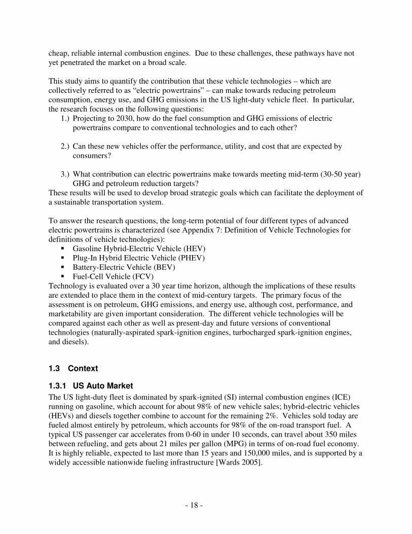
Figure 2: Trends in the US Auto-Market, 1975-2005. Source: EPA 2006a

These market drivers have given rise to the trends shown in Figure 2: Beginning with the enactment of the CAFE standards in 1975, and continuing until the mandated targets reached a plateau in 1987, fuel economy rose dramatically while average vehicle weight and performance both decreased or leveled off. Since that time, 0-60 acceleration has improved by 31% (from 14.5 seconds to 10 seconds), and weight has increased by 28% (from 3200 lbs to 4100 lbs). Over this same period, the light-duty fleet’s fuel economy has actually decreased: although the light-truck and car standards have remained constant, there has been a significant increase in the share of light trucks in the market – rising from a ~20% market share in the 1970’s and early ‘80s to over 50% of the market today. This historical record indicates that, over the last 25 years, while engine technology has gotten steadily more efficient, these efficiency gains have been used to maintain a constant level of fuel economy (within vehicle classes), while simultaneously boosting vehicle power and weight. The nature of this historic performance, size, and fuel economy tradeoff has been quantified by An [2007] and the EPA [2006a]. Because there is little market pull for high efficiency vehicles, each year, as a general rule, OEMs fix sales to meet (rather than exceed) the mandated CAFE standards, and direct technical improvements towards the power and comfort on which passenger vehicles have been more successfully marketed.

1.3.2 Energy and Transportation Policy

With heightened tensions on the petroleum supply and increasing concerns over global warming, the past several years have seen increasing pressure to adopt more stringent regulations to reduce

- 20 -

light-duty transport emissions and petroleum use. However, there have been few substantive changes to create either demand-side pull or supply-side push from OEMs to address these problems. Below is a list which categorizes current or proposed US policy initiatives in the context of the pathways delineated in Table 1. Transportation Policy: Current Status Reduce vehicle-miles traveled: There is little serious effort to undertake an integrated demand-side reduction initiative (using, for example, aggressive gasoline taxes, mileage-based insurance premiums, or urban planning). The primary policy lever in place today is a limited use of gasoline taxes at both the federal and state level to moderate vehicle miles traveled. However, these taxes are primarily justified as a means of funding transportation infrastructure, and are not currently high enough to significantly affect consumer behavior. In fact, even with the gasoline taxes in place, vehicle miles traveled have increased at over 2% per year since 1993 [Davis & Diegel]. Reduce vehicle resistances: There is little serious discussion of reducing vehicle size and weight in the policy context, although there has been a move to tighten the light-truck CAFE standard, which could lead to smaller trucks, or a shift in sales back towards cars. Lightweight vehicles face two big hurdles from the car-buying public: there is a perception that lighter vehicles are less safe, and consumers tend to want larger, roomier cars, which typically increase vehicle weight. Improvements to conventional engine technology: To the extent that the CAFE standards impact fleet fuel economy, they have done so primarily in the context of driving incremental improvements in mainstream technology. However, as discussed above, because the fuel economy standard has remained constant, improvements to mainstream technology have been used to develop larger, more powerful engines which propel larger, faster vehicles. While the 2007 State of the Union called for incrementally increasing CAFE standards by 4% per year, starting in 2010 for cars and 2012 for trucks, until 2017, this has not yet been passed into law [Bush 2007]. Transition to alternative low-carbon, non-petroleum based fuels: Currently, there is a renewable fuels standard that calls for 7.5 billion barrels of bio-fuel to be blended into the gasoline supply by 2012; in his 2007 State of the Union address, President Bush called for a fivefold increase in this mandate to 35 billion barrels by 2017. To the extent that these targets are achieved, they will be met primarily by ethanol derived from corn-based feedstocks. These renewable fuel mandates are problematic both in that there may not be enough cropland to support the mandated ethanol supply without effecting food production, and in that corn-based ethanol delivers only marginal GHG-reduction benefits over petroleum. Longer-term, ethanol derived from cellulosic feedstocks may contribute to the type of integrated solution that is needed, but a viable cellulosic conversion technology may be a decade or more from producing fuel at scale. Transition to new, high-efficiency powertrain concepts: It is hoped that technological advances will enable new incumbents, such as fuel-cell or battery-electric vehicles, to deliver better performance, higher efficiency, zero driving emissions, and comparable cost to present-day mainstream technology – allowing for a compromise-free path to sustainable mobility.

- 21 -

Initiatives aimed at developing these new technologies include both technology-forcing mandates and long-term research and development programs. Examples of the former include the hybrid-electric vehicle (HEV) federal income tax credit, which gives a tax credit of up to $3000 for the purchase of a new HEV, or the California zero-emissions vehicle (ZEV) mandate, which had initially required that 10% of new cars sold in California be zero-emissions vehicles by 2003. The latter was abandoned when it became apparent that the technology was not mature enough to compete in the market. The other important technology-driving effort is the use of public-private partnerships between US OEMs, government agencies, national laboratories, and developers of enabling technologies to focus on long-term, high-risk research into new automotive technologies. Starting in 1993, this research effort fell under the umbrella of the Partnership for Next Generation Vehicles (PNGV), whose goal was to "Build a car with up to 80 miles per gallon at the level of performance, utility and cost of ownership that today's consumers demand." [EERE 2007a] In 2002, the PNGV program was terminated and replaced with the Freedom CAR and Vehicle Technologies (FCVT) program, whose long-term goal is to develop hydrogen-powered fuel cell vehicles and the fuel infrastructure to support them. In a broader sense, FCVT’s seeks to develop “leap frog” technologies that improve energy security, reduce environmental impact, and are less expensive than current day vehicles [EERE 2007b]. The FCVT program also focuses on developing nearer-term technologies that can help enable meeting the program’s long-term goals. Neither program has been successful in meeting its stated end goals, although R&D is ongoing. Transportation Policy: A Broader View In reviewing the above list, an important theme is that this collection of transportation policies does not reflect a coherent long-term plan for addressing the key challenges facing the transport sector. Rather, they reflect a series of political compromises which often lead to market distortions or perverse incentives. Historically, the American populace seems more inclined to regulate industry than to use market-based price signals to drive environmental regulation: an example of this is the use of CAFE standards as the primary policy lever, as opposed to gasoline taxes. These regulatory policies must then be structured so as to gain enough political support among the important concentrated interests to actually get implemented. In many cases, these negotiations result in direct or indirect subsidies to support US industry. For example, the US renewable fuel mandate is often characterized as agricultural, rather than energy policy. In a similar vein, it has been suggested that the stringent US NOx standard that has prevented light-duty diesels from coming to market in the US is an informal trade tariff against European car makers, who possess greater technical expertise in diesel technology than their American counterparts. Likewise, the stagnation in the CAFE standard over the last several decades may be attributable in part to the fact that tightening the standards would disadvantage domestic carmakers relative to their Japanese counterparts. There is also a feeling among many – perhaps justified, perhaps not – that turning the focus to longer-term technological fixes is a way for car makers to avoid making difficult business decisions in the short-term.

- 22 -

$0.00

$500.00

$1,000.00

$1,500.00

$2,000.00

$2,500.00

$3,000.00

$3,500.00

1991

1992

1993

1994

1995

1996

1997

1998

1999

2000

2001

Co

st

($/k

Wh

)

0

20

40

60

80

100

120

140

160

180

Sp

ecif

ic E

nerg

y

(Wh

r/kg

)

Cost Spec. Energy

These political realities and support structures for domestic industry may well be justified. However, with such a complex collection of stakeholders, each with a vested interest in the policy outcome, it can be difficult to gain an accurate or complete perspective on where the realities lie. A key aim of this study is to offer an in-depth, unbiased evaluation of the potential of one path towards developing sustainable mobility. This assessment can then be used to inform the long-term strategic policy decisions that will be likely be made in the next several years.

1.3.3 Electric Powertrains

The rising interest in developing electric powertrains is not merely a function of negative externalities. In parallel with these increasing external pressures, electric powertrains have made significant strides towards competing with conventional technology on their own merits. For example, both battery and fuel-cell technology have improved dramatically in the last decade. These improvements have simultaneously improved performance while decreasing cost.

Figure 3: Improvements in lithium-ion battery technology, 1991-2001 [Adapted from Brodd 2005].

In addition, there is some feeling that electric powertrains can offer a range of attributes, such as

“sportiness”, quiet operation, and a mobile electricity source [Sperling 2004]. Electric utilities also have an interest in deploying grid-charged vehicles, such as plug-in hybrids: a fleet of grid-connected vehicles offers a large energy storage reservoir that can be used to decrease daily variation in the grid and reduce the use of peaking generators on the electric grid – both an economic and environmental boon. None of the technologies under evaluation have yet penetrated the market on any significant scale. Hybrid-electric vehicles (HEV) are in their ascendancy, having established a small but growing niche in the US auto market. In 2006, HEV sales topped 250,000 vehicles and accounted for 1.5% of new vehicle sales. Perhaps just as important, hybrid vehicles have begun to penetrate across vehicle platforms: while early sales were driven largely by sales of the Toyota Prius, in 2006, there were 10 different hybrid models available for purchase, and an additional 6-8 are slated for market introduction by 2009 [hybridcars.com]. With hybridization as a vehicle “option”, it becomes easier and easier for consumers to adopt. Driven primarily by the California zero-emissions vehicle (ZEV) mandate, battery-electric vehicles (BEVs) made a brief foray into the light-duty market during the late 1990s and early 2000s. During this period, several large OEMs (e.g., GM, Toyota, and Honda), produced small

- 23 -

numbers of electric vehicles to test the market; however, support for these programs crumbled due to a combination of lukewarm consumer interest and the end of the ZEV mandate in 2003. More recently, several small (“boutique”) manufacturers have made plans to bring BEVs to market in niche applications; this includes companies such as Tesla, which is developing a high-end electric sports car, and Optima, which offers a small commuter car.

0

4000

8000

12000

16000

20000

24000

28000

Jan '00 Jan '01 Jan '02 Jan '03 Jan '04 Jan '05 Jan '06 Jan '07

Mariner

Escape

Insight

Civic

Accord

Lexus GS

Lexus RX400h

Camry

Highlander

Prius

Figure 4: Hybrid vehicle sales by model and month. Source: Green Car Congress.

Neither plug-in hybrids (PHEVs) nor fuel-cell vehicles have yet been produced for a consumer market. Both are the focus of increasing research and development within both government and industry, and have been deployed in small numbers as test vehicles or as concept cars. While none of these technologies currently constitute a large fraction of vehicles on the road, the high rate of technological development and external market pressures may alter this landscape in the few decades.

1.4 Overview of the Study

Chapter 1 and Chapter 2 provide details on the background, motivation, assumptions, and methodology for this study. Chapter 3 offers a detailed assessment of lithium-ion battery technology into the future and reviews the cross-cutting implications of this evolution with respect to vehicle technology. This analysis finds that cost and durability of batteries are a key sensitivity in the vehicle technology projections. Chapters 4 through 7 present the results of a detailed technical assessment of the different powertrain technologies under evaluation: Chapter 4 will focus on spark-ignition, diesel, and gasoline hybrid-electric vehicles. Chapter 5 focuses on plug-in hybrids, as well as the implications of sourcing transportation energy from the electric grid. Chapter 6 assesses electric vehicles, and chapter 7 deals with fuel-cells. Chapters 9 through 10 present integrated results from the individual technical assessments, draws out the important technology-related and policy-related implications from these results. The study closes with a series of broad, strategic recommendations for addressing energy and environmental issues in the US light-duty transport sector.

- 24 -

2 Methodology

2.1 Overview

It is important to calculate the energy and environmental impacts of the different vehicles on the basis of the full materials lifecycle (“cradle-to-grave”) and fuel-cycle (“well-to-wheel”) of the vehicle. This study focuses primarily on “well-to-wheel” greenhouse gas (GHG) emissions and energy use, which characterizes the energy and emissions associated with fuel use over the vehicle lifetime. This data is calculated in two stages: The “well-to-tank” energy, which accounts for the energy used in refining and transporting fuel from primary sources to the vehicle tank, is determined by reviewing literature from previous studies and applying assumptions appropriate to the context of the 2030 US fleet. The “tank-to-wheel” (or in-use) energy and petroleum use, as well as vehicle performance, are determined from software simulations of vehicle models based on illustrative projections of a year-2030 passenger vehicle. A 2006 2.5L Toyota Camry is used as the basis for the future projections; this vehicle was chosen as a “typical” passenger car because it represented the best-selling vehicle during the model year in question. In addition, its performance and weight are close to the US fleet averages. For completeness, materials lifecycle data is characterized by reviewing previous studies.

2.2 Simulation Methodology

To compare vehicles on an equal footing, vehicle size and performance are held constant at present-day (2006) levels. Specifically, vehicles are equalized in the following dimensions:

“Performance”: This is characterized loosely in terms of 0-60 time, which is set at 9.3 seconds. In addition, vehicles are required to be capable of climbing a 6% grade at 55 MPH, and meeting the US06 (aggressive) drive cycle.

Frontal Area: 2.49 m2 The area and 0-60 time are both fixed to the level of the 2006 2.5L Toyota Camry. The grade climbing criteria was selected as a typical industry grade-climbing requirement. Other vehicle characteristics, such as weight (at constant size), are assumed to improve over time consistent with moderate levels of technological development. Vehicle performance and fuel use were simulated using ADVISOR (ADvanced Vehicle SimulatOR), a Simulink-based software package developed by AVL. ADVISOR is a “backwards facing” vehicle simulator: Given a user-defined vehicle model and schedule of on-road speed requests (a “drive cycle”), it backwards calculates the on-road torque required to meet these requests at each point in time, starting with the wheels, and working backwards through individual drivetrain components to the fuel converter. An illustrative schematic of the Simulink block diagram is shown in Figure 5.

- 25 -

Figure 5: ADVISOR Simulink block diagram.

The vehicle models were developed by integrating individual user-defined component maps into a vehicle that reflects meets the desired performance targets. The methodology and properties used to define component characteristics varies on a case-by-case basis: for some components, such as the vehicle chassis and wheels, evolutionary advances consistent with historical trends were assumed; in other cases, such as for battery or engine technology, a more detailed technical analysis was performed. In general, the logic behind individual design decisions is justified where relevant. These software vehicle models may then be tested against different drive cycles to measure the vehicle’s ability to meet power requests, its fuel use, and its acceleration performance; it also allows the user to track energy flows in the vehicle. For each vehicle under consideration, several different tests were executed: 0-60 Acceleration tests were conducted to equalize performance between vehicles, while three different United States EPA drive cycles were used for testing fuel consumption of vehicles: the FTP (Urban), the HWFET (Highway) drive cycles, and the US06 drive cycle, a more aggressive highway drive cycle. Because the FTP and the HWFET drive cycles understate actual fuel consumption, the EPA specifies that correction factors of 0.9 and 0.78, respectively, be used to adjust the fuel consumption results. In addition to these standard drive cycle tests, limited testing was done using a base accessory load. Two composite cycles were also used in the evaluation: the standard EPA combined cycle, which calculates composite fuel consumption by taking the weighted average of the adjusted FTP (55%) and the adjusted HWFET (45%); and an “industry cycle”, which equally weights the unadjusted HWFET, unadjusted FTP, and US06 cycle. While not actually used by industry, this equal weighting of the three cycles has been shown in previous work to match with somewhat closely with actual proprietary industry test cycles [Natarajan 2002].

2.3 Previous Work

This paper builds closely on several previous studies: “On the Road in 2020” [Weiss 2000], “A Comparative Assessment of Fuel Cell Vehicles” [Weiss 2003], and “Comparative Analysis of Automotive Powertrain Choices for the Near to Mid-Term Future” [Kasseris 2006]. This first two (Weiss 2000 and Weiss 2003) undertook broad-based assessments of vehicle and fuel technologies, projecting vehicle characteristics of both conventional and advanced technology vehicles to the year 2020. This study updates and revises these previous assessments.

- 26 -

More specifically, the ADVISOR software modeling capability is used to undertake a more in depth analysis of vehicle tank-to-wheel performance than these previous studies and update the technology assessment based on recent developments. It also includes an analysis of the plug-in hybrid vehicle, which was not previously modeled. Finally, this study is framed more explicitly as an evaluation of the policy focus in the US on the search for a technological silver bullet to solve the impending transportation challenges. Kasseris [2006] undertook a study of the future evolution of “conventional” automotive technologies – the naturally-aspirated spark-ignition engine, turbocharged spark-ignition engine, diesels, and hybrid-electric vehicles. This previous study develops the methodology and specific underlying vehicles assumptions that are used for modeling vehicles in the current study. These assumptions are discussed in greater depth below. In addition, the results from Kasseris [2006] are used for comparative purposes with the more forward-looking technologies under evaluation, and the hybrid vehicle evaluation is revisited and updated for consistency with the new technologies.

2.4 Assumed Vehicle Characteristics

A number of assumptions developed in previous work [Kasseris 2006] are used as a foundation for this study. These assumptions are summarized below: Vehicle Characteristics: The vehicle chassis is based on an evolved version of the 2006 Toyota Camry. As discussed previously, it is assumed that vehicle size and performance remain constant at 2006 levels. While reducing vehicle resistances – which include aerodynamic drag, tire rolling resistance, and vehicle weight – is not a focus of this study, these parameters, in keeping with historical trends, are likely to improve over time. Accordingly, the aerodynamic drag coefficient is assumed to decrease from 0.28 to 0.21, and tire rolling resistance is assumed to decrease from 0.009 to 0.006. Vehicle weight is also assumed to decrease by ~17% due to incremental materials substitution at constant vehicle size. The specific logic behind these assumptions is detailed in [Kasseris 2006]. Secondary weight assumptions: Additional vehicle weight (from additional components, such as batteries) is assumed to require an additional 50% weight in secondary vehicle support structure, extra engine power, etc. Engine and Transmission: The engine and automatic transmission used in the hybrid and plug-in hybrid vehicles are scaled versions of those used in Kasseris 2006. The transmission used for these vehicles is a 6-speed automatic transmission with manual-transmission like efficiency. The engine is an improved future 4-cylinder spark ignition engine; specific information on the evolution of the engine map and gearbox design are detailed in [Kasseris 2006]. The battery-electric vehicle and fuel-cell vehicles both use a single-speed transmission with incrementally reduced weight from today. Motor/Controller: Each of the vehicles under evaluation requires an electric motor to provide tractive power, either as the prime-mover (as in the fuel-cell or electric vehicle), or to aid with transient power requests (as in the hybrid vehicle). They also require a solid-state power controller to modulate power requests from the battery pack to the motor. Both motor and

- 27 -

controller technology are assumed to improve in line with the goals targeted by the FreedomCAR and Vehicle Technologies (FCVT) Program. A 2004 National Research Council (NRC) review of these targets concluded that meeting the technical targets in the next 10 years is likely. These targets are likely achievable using evolutionarily improved versions of the DC permanent-magnet machines used in present-day hybrids. Specifically, the FCVT targets call for efficiency >93% from 10% to 100% of the motor’s speed range, and specific power (gravimetric power density) of 1.2 kW/kg (including both the motor and controller). To account for tertiary support, a motor/controller specific power of 1.1 kW/kg is used. While more aggressive advancements are certainly feasible, the vehicle models are not very sensitive to specific assumptions about motor characteristics; this is because the motor is a fairly mature technology which already achieves upwards of 90% efficiency over a wide portion of its operating map. The primary areas in which motors and controllers can improve are in terms of cost and volumetric power density – neither of which directly impact vehicle performance or fuel economy. A summary of cross-cutting assumptions is included in Table 2. A more comprehensive table of the relevant vehicle assumptions is included in Appendix 1: Base Case Vehicle Configurations.

Table 2: Assumed vehicle characteristics

Parameter Units Change from 2006 Value Vehicle Parameters

Area m2 0% 2.49

Aero - -25% 0.21

Rolling - -33% 0.006

Weight Assumptions

Vehicle Wt Kg -20% 1148

Transmission Weight Kg -20% 92

Specific Power, Engine kW/kg 20% 0.925

Specific Power, Motor kW/kg 30% 1.1

Efficiency Assumptions

Peak indicative ηEngine % 7.5% 43%

Peak ηMotor/Controller % 6% 95%

ηTransmission % 5.6% 94%

2.5 Cost Methodology

While this study does not perform original cost-modeling, care has been taken to review the appropriate literature and engage in conversation with experts from industry to get a sense of the future costs of different vehicle technologies. The costs of future vehicle technologies are calculated by summing the incremental cost or cost credit on a component-by-component basis of major vehicle sub-systems as compared to the 2030 naturally-aspirated spark-ignition engine. All costs reflect the cost to the OEM. Specific cost assumptions are discussed in the relevant chapter throughout this thesis, while an integrated table of assumptions, sources, and costs is presented in section 8.2.

- 28 -

2.6 Well-to-Tank Energy Use and GHG Emissions

Table 3: Assumed energy and carbon content of different fuel sources. Data is expressed in terms of the amount of energy or CO2 equivalent released to deliver 1 MJ of fuel to the tank.

Fuel Energy (MJ/MJ, LHV)

GHG Emissions Rate (g CO2/MJ)

Well-to-Tank Tank-to-Wheel Gasoline 0.24 21.2 71.9

Diesel 0.14 12.0 76.3

Hydrogen 0.84 115.2 0.0

Electricity (2030 Avg Grid)

2.30 213.6 0.0

Table 3 shows the energy use and GHG emissions associated with producing and using different transportation fuels. The data in this table is interpreted as follows:

Energy: The amount of energy it takes to deliver 1 MJ of energy to the fuel tank of the car, based on the lower heating value (LHV) of the fuel in question.

Well-to-Tank GHG Emissions Rate: The amount of greenhouse gases (GHGs), in CO2-

equivalent, emitted per MJ of energy used in producing the fuel. Hence, to calculate the GHG emissions per MJ in the tank, one would multiply the first column by the second column.

Tank-to-Wheel GHG Emissions Rate: The amount of GHGs, in CO2-equivalent,

released from using 1 MJ of fuel in the tank. The well-to-tank energy and emissions associated with refining and transporting gasoline are taken from the GM/ANL GREET study [GM/ANL 2005]; the diesel data is from Weiss [2000]2. These assumptions are also used for calculating upstream energy and emissions associated with producing Hydrogen. The hydrogen fuel cycle data assumes that hydrogen is produced by steam-reforming gaseous North American natural gas at distributed locations, and is compressed to 10K PSI; these assumptions are discussed in greater detail in Section 7.4. The electricity assumptions are based on the more in-depth assessment of the emissions impact of plug-in vehicles on the electric grid from Chapter 5.7, although the analysis concludes that the average grid mix projected by the 2030 EIA Annual Energy Outlook is an appropriate estimate.

2.7 Embodied Vehicle Energy: Cradle-to-Grave Energy Use

Although not a focus of this study, the energy used to manufacture and recycled a vehicle – the embodied energy – is an important consideration when characterizing the total vehicle lifecycle energy use. It is particularly relevant when comparing vehicle technologies which require

2 The GREET diesel data differs by a wide margin (1.5X) from other similar studies of diesel tank-to-wheel data. These differences arise from different assumptions about refining energy which go beyond increases due to desulfurization. Because other studies seem to converge at the lower value, they are used. For reference, the relevant diesel WTT data from GREET is .21 MJ/MJ in the tank and 19 g CO2/MJ.

- 29 -

fundamentally different materials and manufacturing processes – in particular, batteries and fuel-cells. A recent study out of Argonne National Labs (ANL) [Moon et al 2006] modeled the embodied energy and GHG emissions for a range of vehicle technologies. Their results estimate that vehicle embodied energy accounts for about 21% of total lifecycle GHG emissions and 18% of total energy use in a conventional spark-ignition vehicle – a sizeable piece of the total. However, the difference between different powertrain technologies is only a fraction of this amount. Figure 6 shows the change in lifecycle energy, relative to the NA-SI engine, for different technologies. In the case of the hybrid and plug-in hybrid vehicle, there is little change. While there are non-trivial differences in the manufacturing energy used for these vehicles, the differences are masked by the fact that this embodied energy is only 20% of the total – hence, it is a fraction of a fraction. In the case of the fuel-cell vehicle, the difference is much more pronounced. Although the battery-electric vehicle was not modeled, it would presumably fall somewhere between the FCV and the PHEV (probably closer to the FCV, due to its large battery pack). It is likely that advances in fuel-cell technology, such as higher power density, can reduce this extra manufacturing energy in the future.

Change in GHG/Energy relative to ICE due to Embodied Eenergy

0.0%

1.0%

2.0%

3.0%

4.0%

5.0%

6.0%

7.0%

8.0%

9.0%

HEV PHEV FCV

GHG

Energy

Figure 6: Change in total lifecycle GHG emissions/energy use relative to the NA-SI due to the embodied energy.

This analysis suggests that differences in lifecycle energy are relatively negligible in the context of the hybrid and plug-in hybrid, but may be an important consideration for the fuel-cell and battery-electric vehicles. This data is presented for reference, but is not considered within the overall context of the paper. Rather, it is treated as an important additional consideration when evaluating between different powertrains.

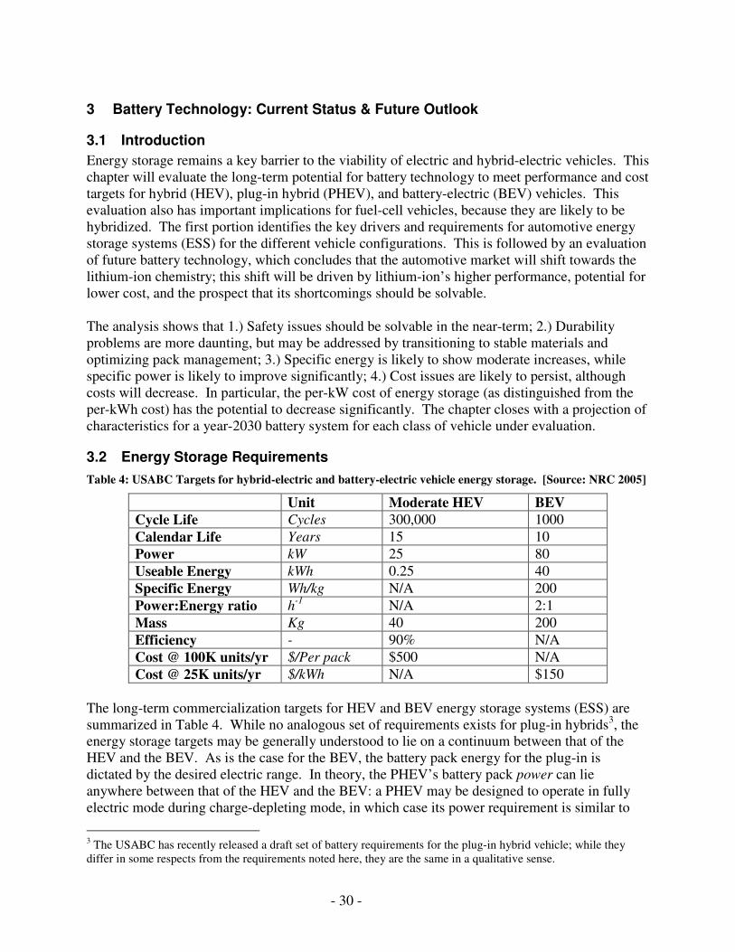
- 30 -

3 Battery Technology: Current Status & Future Outlook

3.1 Introduction

Energy storage remains a key barrier to the viability of electric and hybrid-electric vehicles. This chapter will evaluate the long-term potential for battery technology to meet performance and cost targets for hybrid (HEV), plug-in hybrid (PHEV), and battery-electric (BEV) vehicles. This evaluation also has important implications for fuel-cell vehicles, because they are likely to be hybridized. The first portion identifies the key drivers and requirements for automotive energy storage systems (ESS) for the different vehicle configurations. This is followed by an evaluation of future battery technology, which concludes that the automotive market will shift towards the lithium-ion chemistry; this shift will be driven by lithium-ion’s higher performance, potential for lower cost, and the prospect that its shortcomings should be solvable. The analysis shows that 1.) Safety issues should be solvable in the near-term; 2.) Durability problems are more daunting, but may be addressed by transitioning to stable materials and optimizing pack management; 3.) Specific energy is likely to show moderate increases, while specific power is likely to improve significantly; 4.) Cost issues are likely to persist, although costs will decrease. In particular, the per-kW cost of energy storage (as distinguished from the per-kWh cost) has the potential to decrease significantly. The chapter closes with a projection of characteristics for a year-2030 battery system for each class of vehicle under evaluation.

3.2 Energy Storage Requirements

Table 4: USABC Targets for hybrid-electric and battery-electric vehicle energy storage. [Source: NRC 2005]

Unit Moderate HEV BEV Cycle Life Cycles 300,000 1000

Calendar Life Years 15 10

Power kW 25 80

Useable Energy kWh 0.25 40

Specific Energy Wh/kg N/A 200

Power:Energy ratio h-1 N/A 2:1

Mass Kg 40 200

Efficiency - 90% N/A

Cost @ 100K units/yr $/Per pack $500 N/A

Cost @ 25K units/yr $/kWh N/A $150

The long-term commercialization targets for HEV and BEV energy storage systems (ESS) are summarized in Table 4. While no analogous set of requirements exists for plug-in hybrids3, the energy storage targets may be generally understood to lie on a continuum between that of the HEV and the BEV. As is the case for the BEV, the battery pack energy for the plug-in is dictated by the desired electric range. In theory, the PHEV’s battery pack power can lie anywhere between that of the HEV and the BEV: a PHEV may be designed to operate in fully electric mode during charge-depleting mode, in which case its power requirement is similar to

3 The USABC has recently released a draft set of battery requirements for the plug-in hybrid vehicle; while they differ in some respects from the requirements noted here, they are the same in a qualitative sense.

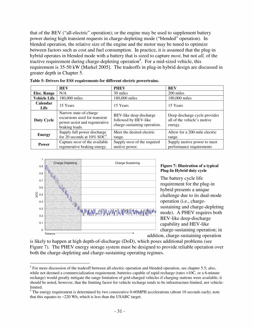
- 31 -

0

0.1

0.2

0.3

0.4

0.5

0.6

0.7

0.8

0.9

1

Distance

SO

C

Charge-Depleting Charge-Sustaining

that of the BEV (“all-electric” operation); or the engine may be used to supplement battery power during high transient requests in charge-depleting mode (“blended” operation). In blended operation, the relative size of the engine and the motor may be tuned to optimize between factors such as cost and fuel consumption. In practice, it is assumed that the plug-in hybrid operates in blended mode with a battery that is sized to capture most, but not all, of the tractive requirement during charge-depleting operation4. For a mid-sized vehicle, this requirement is 35-50 kW [Markel 2005]. The tradeoffs in plug-in hybrid design are discussed in greater depth in Chapter 5.

Table 5: Drivers for ESS requirements for different electric powertrains.

HEV PHEV BEV

Elec. Range N/A 30 miles 200 miles

Vehicle Life 180,000 miles 180,000 miles 180,000 miles

Calendar Life

15 Years 15 Years 15 Years

Duty Cycle

Narrow state-of-charge excursions used for transient power-assist and regenerative braking loads.

BEV-like deep discharge followed by HEV-like charge-sustaining operation.

Deep discharge cycle provides all of the vehicle’s motive energy.

Energy Supply full power discharge for 20 seconds at 10% SOC5.

Meet the desired electric range.

Allow for a 200-mile electric range.

Power Capture most of the available regenerative braking energy.

Supply most of the required motive power.

Supply motive power to meet performance requirements

Figure 7: Illustration of a typical Plug-In Hybrid duty cycle

The battery cycle life requirement for the plug-in hybrid presents a unique challenge due to its dual-mode operation (i.e., charge-sustaining and charge-depleting mode). A PHEV requires both BEV-like deep-discharge capability and HEV-like charge-sustaining operation; in

addition, charge-sustaining operation is likely to happen at high depth-of-discharge (DoD), which poses additional problems (see Figure 7). The PHEV energy storage system must be designed to provide reliable operation over both the charge-depleting and charge-sustaining operating regimes.

4 For more discussion of the tradeoff between all-electric operation and blended operation, see chapter 5.5; also, while not deemed a commercialization requirement, batteries capable of rapid recharge (rates >10C, or a 6-minute recharge) would greatly mitigate the range limitation of grid-charged vehicles if charging stations were available; it should be noted, however, that the limiting factor for vehicle recharge tends to be infrastructure-limited, not vehicle-limited. 5 The energy requirement is determined by two consecutive 0-60MPH accelerations (about 10 seconds each); note that this equates to ~220 Wh, which is less than the USABC target.

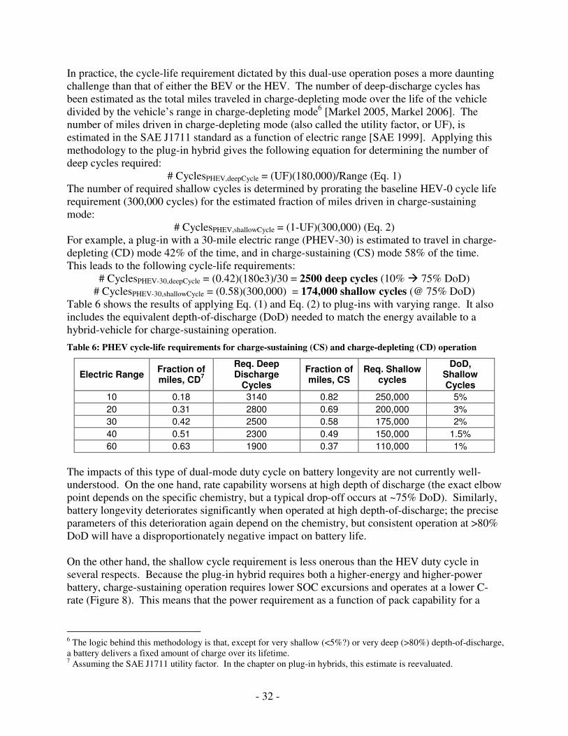
- 32 -

In practice, the cycle-life requirement dictated by this dual-use operation poses a more daunting challenge than that of either the BEV or the HEV. The number of deep-discharge cycles has been estimated as the total miles traveled in charge-depleting mode over the life of the vehicle divided by the vehicle’s range in charge-depleting mode6 [Markel 2005, Markel 2006]. The number of miles driven in charge-depleting mode (also called the utility factor, or UF), is estimated in the SAE J1711 standard as a function of electric range [SAE 1999]. Applying this methodology to the plug-in hybrid gives the following equation for determining the number of deep cycles required:

# CyclesPHEV,deepCycle = (UF)(180,000)/Range (Eq. 1) The number of required shallow cycles is determined by prorating the baseline HEV-0 cycle life requirement (300,000 cycles) for the estimated fraction of miles driven in charge-sustaining mode:

# CyclesPHEV,shallowCycle = (1-UF)(300,000) (Eq. 2) For example, a plug-in with a 30-mile electric range (PHEV-30) is estimated to travel in charge-depleting (CD) mode 42% of the time, and in charge-sustaining (CS) mode 58% of the time. This leads to the following cycle-life requirements:

# CyclesPHEV-30,deepCycle = (0.42)(180e3)/30 = 2500 deep cycles (10% 75% DoD) # CyclesPHEV-30,shallowCycle = (0.58)(300,000) = 174,000 shallow cycles (@ 75% DoD)

Table 6 shows the results of applying Eq. (1) and Eq. (2) to plug-ins with varying range. It also includes the equivalent depth-of-discharge (DoD) needed to match the energy available to a hybrid-vehicle for charge-sustaining operation.

Table 6: PHEV cycle-life requirements for charge-sustaining (CS) and charge-depleting (CD) operation

Electric Range Fraction of miles, CD

7

Req. Deep Discharge

Cycles

Fraction of miles, CS

Req. Shallow cycles

DoD, Shallow Cycles

10 0.18 3140 0.82 250,000 5%

20 0.31 2800 0.69 200,000 3%

30 0.42 2500 0.58 175,000 2%

40 0.51 2300 0.49 150,000 1.5%

60 0.63 1900 0.37 110,000 1%

The impacts of this type of dual-mode duty cycle on battery longevity are not currently well-understood. On the one hand, rate capability worsens at high depth of discharge (the exact elbow point depends on the specific chemistry, but a typical drop-off occurs at ~75% DoD). Similarly, battery longevity deteriorates significantly when operated at high depth-of-discharge; the precise parameters of this deterioration again depend on the chemistry, but consistent operation at >80% DoD will have a disproportionately negative impact on battery life. On the other hand, the shallow cycle requirement is less onerous than the HEV duty cycle in several respects. Because the plug-in hybrid requires both a higher-energy and higher-power battery, charge-sustaining operation requires lower SOC excursions and operates at a lower C-rate (Figure 8). This means that the power requirement as a function of pack capability for a

6 The logic behind this methodology is that, except for very shallow (<5%?) or very deep (>80%) depth-of-discharge, a battery delivers a fixed amount of charge over its lifetime. 7 Assuming the SAE J1711 utility factor. In the chapter on plug-in hybrids, this estimate is reevaluated.

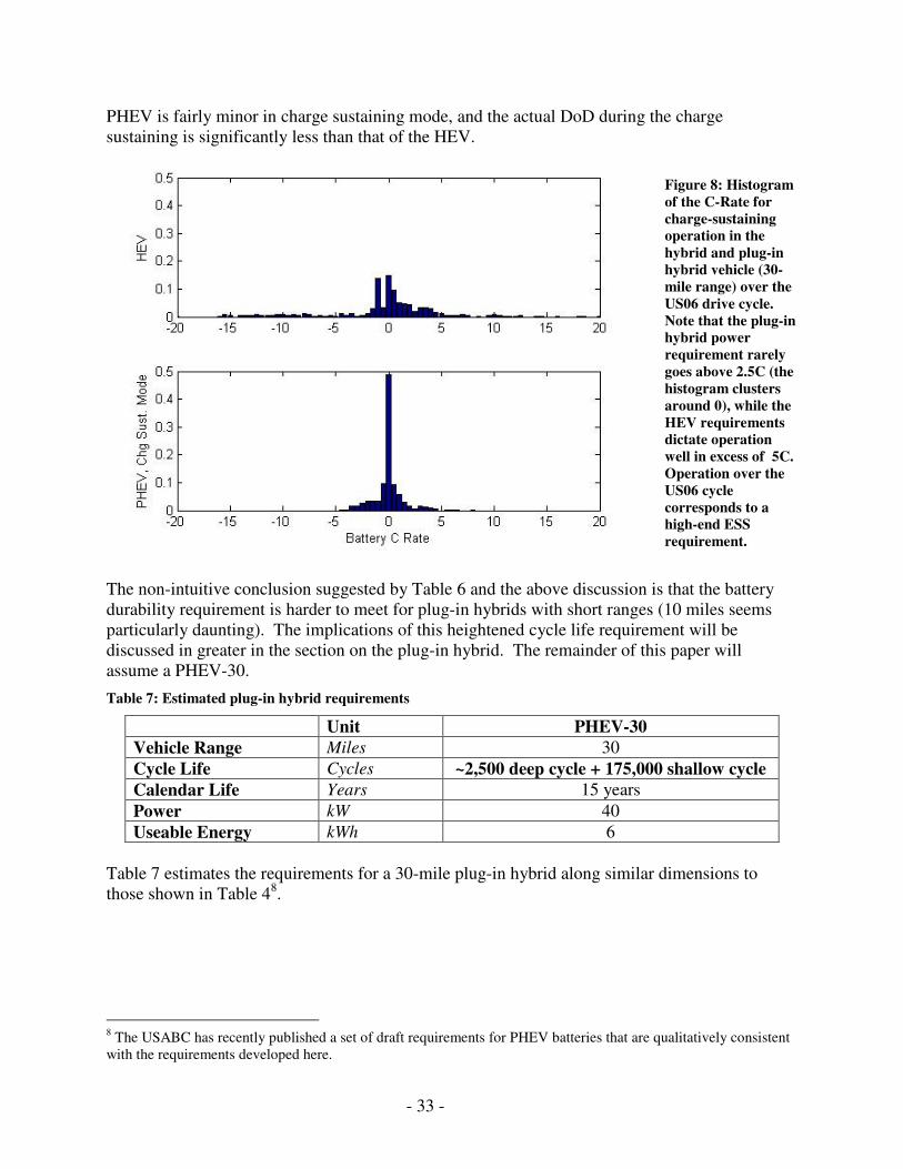
- 33 -

PHEV is fairly minor in charge sustaining mode, and the actual DoD during the charge sustaining is significantly less than that of the HEV.

Figure 8: Histogram of the C-Rate for charge-sustaining operation in the hybrid and plug-in hybrid vehicle (30-mile range) over the US06 drive cycle. Note that the plug-in hybrid power requirement rarely goes above 2.5C (the histogram clusters around 0), while the HEV requirements dictate operation well in excess of 5C. Operation over the US06 cycle corresponds to a high-end ESS requirement.

The non-intuitive conclusion suggested by Table 6 and the above discussion is that the battery durability requirement is harder to meet for plug-in hybrids with short ranges (10 miles seems particularly daunting). The implications of this heightened cycle life requirement will be discussed in greater in the section on the plug-in hybrid. The remainder of this paper will assume a PHEV-30.

Table 7: Estimated plug-in hybrid requirements

Unit PHEV-30 Vehicle Range Miles 30

Cycle Life Cycles ~2,500 deep cycle + 175,000 shallow cycle Calendar Life Years 15 years

Power kW 40

Useable Energy kWh 6

Table 7 estimates the requirements for a 30-mile plug-in hybrid along similar dimensions to those shown in Table 48.

8 The USABC has recently published a set of draft requirements for PHEV batteries that are qualitatively consistent with the requirements developed here.

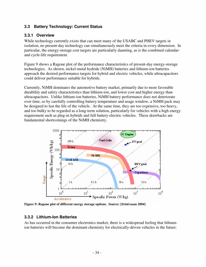
- 34 -

3.3 Battery Technology: Current Status

3.3.1 Overview

While technology currently exists that can meet many of the USABC and PHEV targets in isolation, no present-day technology can simultaneously meet the criteria in every dimension. In particular, the energy-storage cost targets are particularly daunting, as is the combined calendar- and cycle-life requirement. Figure 9 shows a Ragone plot of the performance characteristics of present-day energy-storage technologies. As shown, nickel-metal hydride (NiMH) batteries and lithium-ion batteries approach the desired performance targets for hybrid and electric vehicles, while ultracapacitors could deliver performance suitable for hybrids. Currently, NiMH dominates the automotive battery market, primarily due to more favorable durability and safety characteristics than lithium-ion, and lower cost and higher energy than ultracapacitors. Unlike lithium-ion batteries, NiMH battery performance does not deteriorate over time, so by carefully controlling battery temperature and usage window, a NiMH pack may be designed to last the life of the vehicle. At the same time, they are too expensive, too heavy, and too bulky to be regarded as a long-term solution, particularly for vehicles with a high energy requirement such as plug-in hybrids and full battery-electric vehicles. These drawbacks are fundamental shortcomings of the NiMH chemistry.

Figure 9: Ragone plot of different energy storage options. Source: [Srinivasan 2004]

3.3.2 Lithium-Ion Batteries

As has occurred in the consumer electronics market, there is a widespread feeling that lithium-ion batteries will become the dominant chemistry for electrically-driven vehicles in the future:

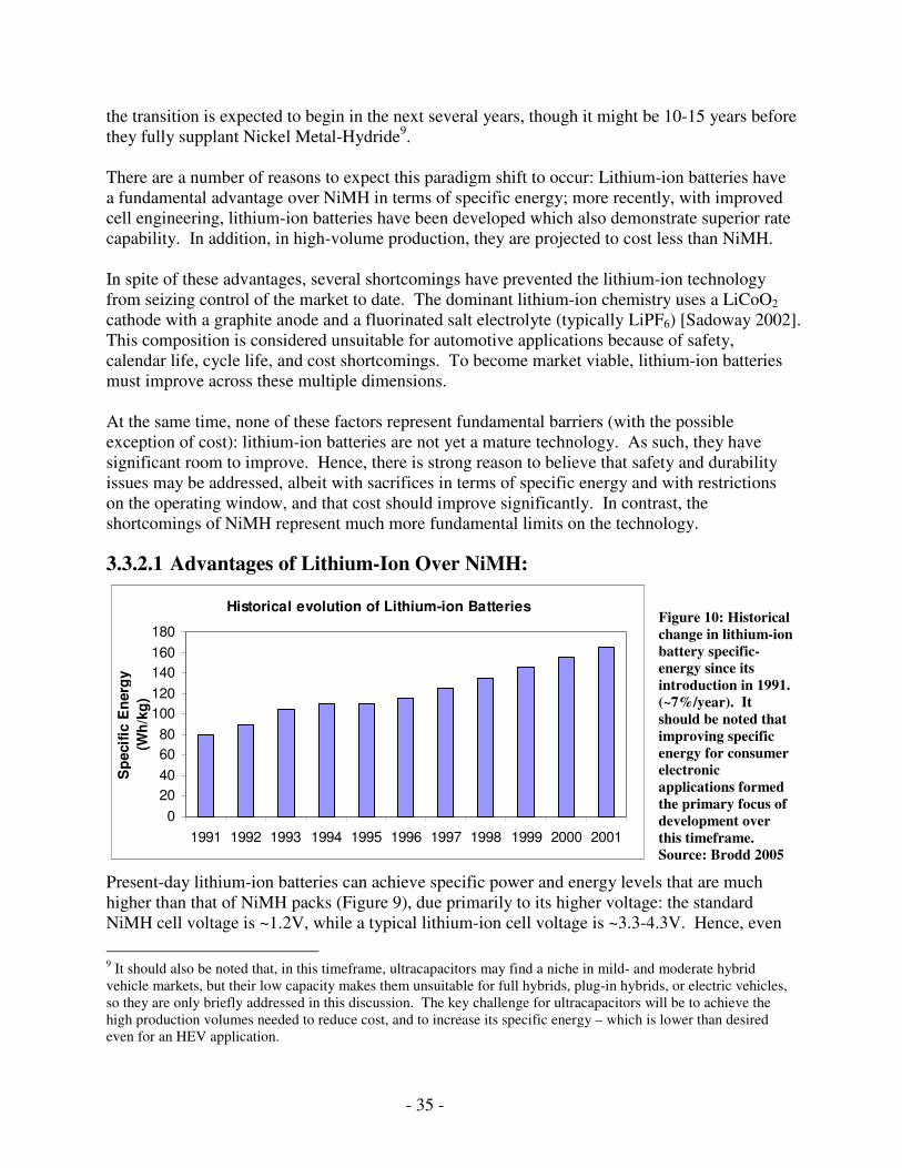
- 35 -

Historical evolution of Lithium-ion Batteries

0

20

40

60

80

100

120

140

160

180

1991 1992 1993 1994 1995 1996 1997 1998 1999 2000 2001

Sp

ecif

ic E

nerg

y

(Wh

/kg

)

the transition is expected to begin in the next several years, though it might be 10-15 years before they fully supplant Nickel Metal-Hydride9. There are a number of reasons to expect this paradigm shift to occur: Lithium-ion batteries have a fundamental advantage over NiMH in terms of specific energy; more recently, with improved cell engineering, lithium-ion batteries have been developed which also demonstrate superior rate capability. In addition, in high-volume production, they are projected to cost less than NiMH. In spite of these advantages, several shortcomings have prevented the lithium-ion technology from seizing control of the market to date. The dominant lithium-ion chemistry uses a LiCoO2 cathode with a graphite anode and a fluorinated salt electrolyte (typically LiPF6) [Sadoway 2002]. This composition is considered unsuitable for automotive applications because of safety, calendar life, cycle life, and cost shortcomings. To become market viable, lithium-ion batteries must improve across these multiple dimensions. At the same time, none of these factors represent fundamental barriers (with the possible exception of cost): lithium-ion batteries are not yet a mature technology. As such, they have significant room to improve. Hence, there is strong reason to believe that safety and durability issues may be addressed, albeit with sacrifices in terms of specific energy and with restrictions on the operating window, and that cost should improve significantly. In contrast, the shortcomings of NiMH represent much more fundamental limits on the technology.

3.3.2.1 Advantages of Lithium-Ion Over NiMH:

Figure 10: Historical change in lithium-ion battery specific-energy since its introduction in 1991. (~7%/year). It should be noted that improving specific energy for consumer electronic applications formed the primary focus of development over this timeframe. Source: Brodd 2005

Present-day lithium-ion batteries can achieve specific power and energy levels that are much higher than that of NiMH packs (Figure 9), due primarily to its higher voltage: the standard NiMH cell voltage is ~1.2V, while a typical lithium-ion cell voltage is ~3.3-4.3V. Hence, even

9 It should also be noted that, in this timeframe, ultracapacitors may find a niche in mild- and moderate hybrid vehicle markets, but their low capacity makes them unsuitable for full hybrids, plug-in hybrids, or electric vehicles, so they are only briefly addressed in this discussion. The key challenge for ultracapacitors will be to achieve the high production volumes needed to reduce cost, and to increase its specific energy – which is lower than desired even for an HEV application.

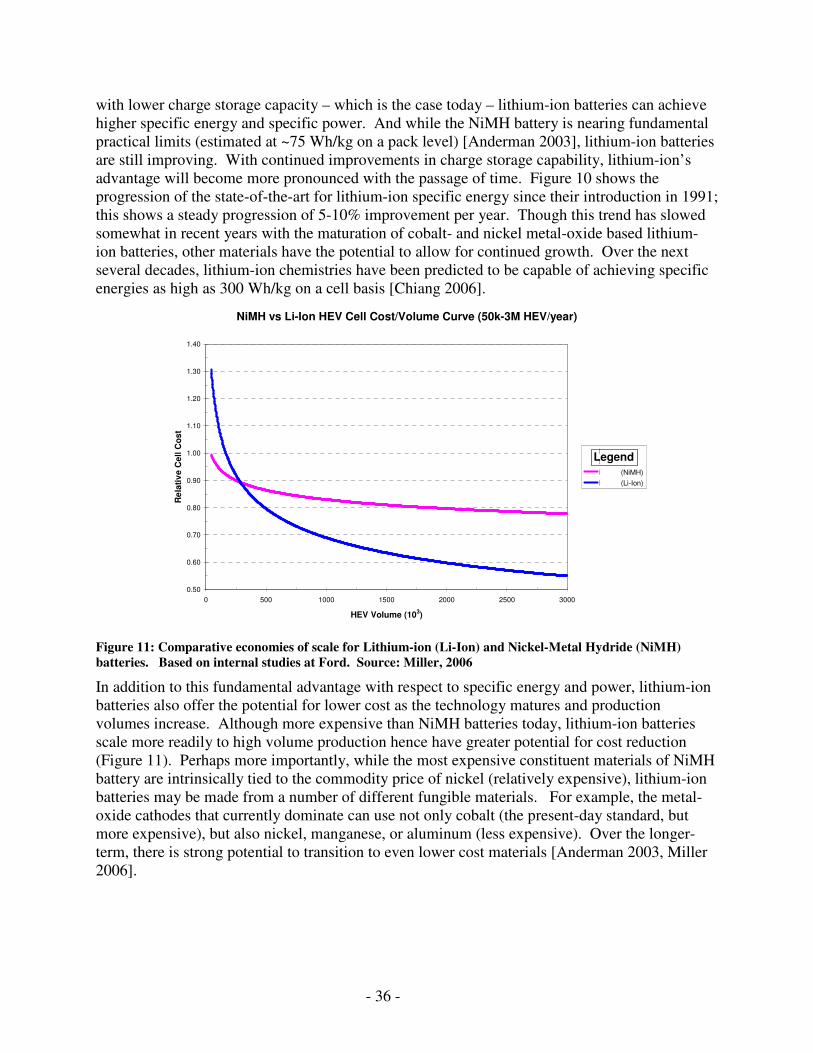
- 36 -

with lower charge storage capacity – which is the case today – lithium-ion batteries can achieve higher specific energy and specific power. And while the NiMH battery is nearing fundamental practical limits (estimated at ~75 Wh/kg on a pack level) [Anderman 2003], lithium-ion batteries are still improving. With continued improvements in charge storage capability, lithium-ion’s advantage will become more pronounced with the passage of time. Figure 10 shows the progression of the state-of-the-art for lithium-ion specific energy since their introduction in 1991; this shows a steady progression of 5-10% improvement per year. Though this trend has slowed somewhat in recent years with the maturation of cobalt- and nickel metal-oxide based lithium-ion batteries, other materials have the potential to allow for continued growth. Over the next several decades, lithium-ion chemistries have been predicted to be capable of achieving specific energies as high as 300 Wh/kg on a cell basis [Chiang 2006].

Figure 11: Comparative economies of scale for Lithium-ion (Li-Ion) and Nickel-Metal Hydride (NiMH) batteries. Based on internal studies at Ford. Source: Miller, 2006

In addition to this fundamental advantage with respect to specific energy and power, lithium-ion batteries also offer the potential for lower cost as the technology matures and production volumes increase. Although more expensive than NiMH batteries today, lithium-ion batteries scale more readily to high volume production hence have greater potential for cost reduction (Figure 11). Perhaps more importantly, while the most expensive constituent materials of NiMH battery are intrinsically tied to the commodity price of nickel (relatively expensive), lithium-ion batteries may be made from a number of different fungible materials. For example, the metal-oxide cathodes that currently dominate can use not only cobalt (the present-day standard, but more expensive), but also nickel, manganese, or aluminum (less expensive). Over the longer-term, there is strong potential to transition to even lower cost materials [Anderman 2003, Miller 2006].

NiMH vs Li-Ion HEV Cell Cost/Volume Curve (50k-3M HEV/year)

0.50

0.60

0.70

0.80

0.90

1.00

1.10

1.20

1.30

1.40

0 500 1000 1500 2000 2500 3000

HEV Volume (103)

Re

lati

ve

Ce

ll C

os

t

Li-Ion

NiMH

Power (NiMH)

Power (Li-Ion)

Legend

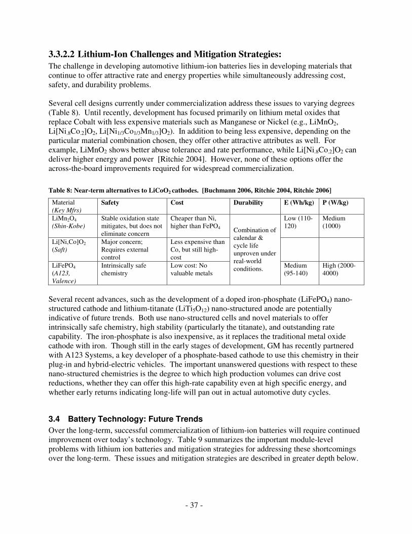
- 37 -

3.3.2.2 Lithium-Ion Challenges and Mitigation Strategies:

The challenge in developing automotive lithium-ion batteries lies in developing materials that continue to offer attractive rate and energy properties while simultaneously addressing cost, safety, and durability problems. Several cell designs currently under commercialization address these issues to varying degrees (Table 8). Until recently, development has focused primarily on lithium metal oxides that replace Cobalt with less expensive materials such as Manganese or Nickel (e.g., LiMnO2, Li[Ni.8Co.2]O2, Li[Ni1/3Co1/3Mn1/3]O2). In addition to being less expensive, depending on the particular material combination chosen, they offer other attractive attributes as well. For example, LiMnO2 shows better abuse tolerance and rate performance, while Li[Ni.8Co.2]O2 can deliver higher energy and power [Ritchie 2004]. However, none of these options offer the across-the-board improvements required for widespread commercialization.

Table 8: Near-term alternatives to LiCoO2 cathodes. [Buchmann 2006, Ritchie 2004, Ritchie 2006]

Material (Key Mfrs)

Safety Cost Durability E (Wh/kg) P (W/kg)

LiMn2O4

(Shin-Kobe) Stable oxidation state mitigates, but does not eliminate concern

Cheaper than Ni, higher than FePO4

Low (110-120)

Medium (1000)

Li[Ni,Co]O2 (Saft)

Major concern; Requires external control

Less expensive than Co, but still high-cost

LiFePO4 (A123, Valence)

Intrinsically safe chemistry

Low cost: No valuable metals

Combination of calendar & cycle life unproven under real-world conditions.

Medium (95-140)

High (2000-4000)

Several recent advances, such as the development of a doped iron-phosphate (LiFePO4) nano-structured cathode and lithium-titanate (LiTi5O12) nano-structured anode are potentially indicative of future trends. Both use nano-structured cells and novel materials to offer intrinsically safe chemistry, high stability (particularly the titanate), and outstanding rate capability. The iron-phosphate is also inexpensive, as it replaces the traditional metal oxide cathode with iron. Though still in the early stages of development, GM has recently partnered with A123 Systems, a key developer of a phosphate-based cathode to use this chemistry in their plug-in and hybrid-electric vehicles. The important unanswered questions with respect to these nano-structured chemistries is the degree to which high production volumes can drive cost reductions, whether they can offer this high-rate capability even at high specific energy, and whether early returns indicating long-life will pan out in actual automotive duty cycles.

3.4 Battery Technology: Future Trends

Over the long-term, successful commercialization of lithium-ion batteries will require continued improvement over today’s technology. Table 9 summarizes the important module-level problems with lithium ion batteries and mitigation strategies for addressing these shortcomings over the long-term. These issues and mitigation strategies are described in greater depth below.

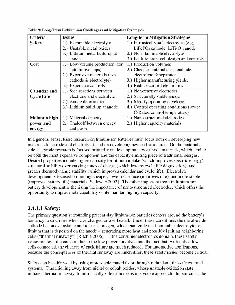
- 38 -

Table 9: Long-Term Lithium-ion Challenges and Mitigation Strategies

Criteria Issues Long-term Mitigation Strategies Safety 1.) Flammable electrolyte

2.) Unstable metal oxides 3.) Lithium metal build-up at

anode.

1.) Intrinsically safe electrodes (e.g, LiFePO4 cathode; LiTi5O12 anode)

2.) Non-flammable electrolyte 3.) Fault-tolerant cell design and controls.

Cost 1.) Low-volume production (for automotive apps)

2.) Expensive materials (esp cathode & electrolyte)

3.) Expensive controls

1.) Production volumes 2.) Cheaper materials, esp cathode,

electrolyte & separator 3.) Higher manufacturing yields. 4.) Reduce control electronics

Calendar and Cycle Life

1.) Side reactions between electrode and electrolyte

2.) Anode deformation 3.) Lithium build-up at anode

1.) Non-reactive electrodes 2.) Structurally stable anode 3.) Modify operating envelope 4.) Control operating conditions (lower

C-Rates, control temperature)

Maintain high power and energy

1.) Material capacity 2.) Tradeoff between energy

and power

1.) Nano-structured electrodes 2.) Higher capacity materials

In a general sense, basic research on lithium-ion batteries must focus both on developing new materials (electrode and electrolyte), and on developing new cell structures. On the materials side, electrode research is focused primarily on developing new cathode materials, which tend to be both the most expensive component and the capacity-limiting piece of traditional designs. Desired properties include higher capacity for lithium uptake (which improves specific energy); structural stability over varying states of charge (which lessens cycle life degradation); and greater thermodynamic stability (which improves calendar and cycle life). Electrolyte development is focused on finding cheaper, lower resistance (improves rate), and more stable (improves battery life) materials [Sadoway 2002]. The other important trend in lithium-ion battery development is the rising the importance of nano-structured electrodes, which offers the opportunity to improve rate capability while maintaining high capacity.

3.4.1.1 Safety:

The primary question surrounding present-day lithium-ion batteries centers around the battery’s tendency to catch fire when overcharged or overheated. Under these conditions, the metal-oxide cathode becomes unstable and releases oxygen, which can ignite the flammable electrolyte or lithium that is deposited on the anode – generating more heat and possibly igniting neighboring cells (“thermal runaway”) [Ritchie 2006]. In the consumer electronics domain, these safety issues are less of a concern due to the low powers involved and the fact that, with only a few cells connected, the chances of pack failure are much reduced. For automotive applications, because the consequences of thermal runaway are much direr, these safety issues become critical. Safety can be addressed by using more stable materials or through redundant, fail-safe external systems. Transitioning away from nickel or cobalt oxides, whose unstable oxidation state initiates thermal runaway, to intrinsically safe cathodes is one viable approach. In particular, the

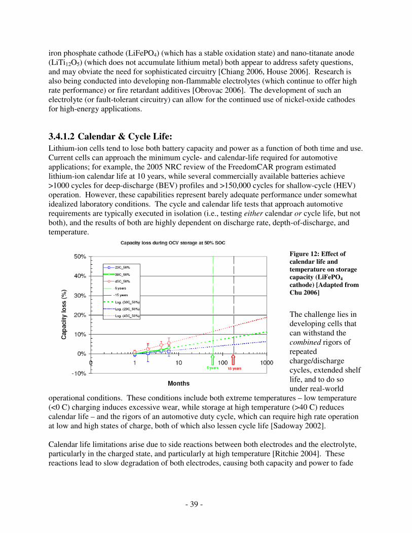
- 39 -

iron phosphate cathode (LiFePO4) (which has a stable oxidation state) and nano-titanate anode (LiTi12O5) (which does not accumulate lithium metal) both appear to address safety questions, and may obviate the need for sophisticated circuitry [Chiang 2006, House 2006]. Research is also being conducted into developing non-flammable electrolytes (which continue to offer high rate performance) or fire retardant additives [Obrovac 2006]. The development of such an electrolyte (or fault-tolerant circuitry) can allow for the continued use of nickel-oxide cathodes for high-energy applications.

3.4.1.2 Calendar & Cycle Life:

Lithium-ion cells tend to lose both battery capacity and power as a function of both time and use. Current cells can approach the minimum cycle- and calendar-life required for automotive applications; for example, the 2005 NRC review of the FreedomCAR program estimated lithium-ion calendar life at 10 years, while several commercially available batteries achieve >1000 cycles for deep-discharge (BEV) profiles and >150,000 cycles for shallow-cycle (HEV) operation. However, these capabilities represent barely adequate performance under somewhat idealized laboratory conditions. The cycle and calendar life tests that approach automotive requirements are typically executed in isolation (i.e., testing either calendar or cycle life, but not both), and the results of both are highly dependent on discharge rate, depth-of-discharge, and temperature.

Figure 12: Effect of calendar life and temperature on storage capacity (LiFePO4 cathode) [Adapted from Chu 2006]

The challenge lies in developing cells that can withstand the combined rigors of repeated charge/discharge cycles, extended shelf life, and to do so under real-world

operational conditions. These conditions include both extreme temperatures – low temperature (<0 C) charging induces excessive wear, while storage at high temperature (>40 C) reduces calendar life – and the rigors of an automotive duty cycle, which can require high rate operation at low and high states of charge, both of which also lessen cycle life [Sadoway 2002]. Calendar life limitations arise due to side reactions between both electrodes and the electrolyte, particularly in the charged state, and particularly at high temperature [Ritchie 2004]. These reactions lead to slow degradation of both electrodes, causing both capacity and power to fade

- 40 -

with time. Hence, calendar life degradation is largely a function of the reactivity of the electrodes with the electrolyte. Cycle life degradation arises from deposition of lithium metal on the anode, which causes both impedance growth (due to reduced surface area of the electrode) and reduced capacity (due to reduction in the quantity of active material) [Broussley 2005]. In addition, problems arise from deformation of the anode’s crystalline structure during repeated cycling [House 2006]. These problems are particularly pronounced at high rate and low state of charge (SOC): high rates can overrun the material’s lithium uptake capability, causing plating, while low SOC incurs particularly pronounced crystalline deformation. These durability issues can be addressed either by modifying usage to reduce strain on the battery, or by transitioning to new materials with more favorable properties. In practice, both of these approaches are likely to be employed. Problems with cycle life may be effectively mitigated by over-sizing the battery pack in either the energy dimension (and operating in a restricted state-of-charge envelope) or the power dimension (allowing for lower C-rates). The drawback to this approach is that it is expensive, so the optimum strategy entails tuning the battery operating window to the required usage pattern and lifetime. (For example, a hybrid vehicle, which requires several hundred thousand cycles, is designed to operate within a narrow SOC band, while a BEV would operate to a high depth-of-discharge). In theory, calendar life may be extended by storing the battery at low temperature and at less than full charge. In practice, these calendar-life mitigation strategies are problematic, as there is no way to rigorously control for these parameters in the automotive sector. The issue may be partially mitigated by recharging the battery to just below the maximum capacity. On the materials side, durability may be improved by finding combinations of electrodes and electrolytes that do not react with each other, and anodes that are, in addition to being non-reactive, show minimal deformation. The lithium-titanate anode shows excellent performance in this respect (virtually eliminating cycle-life degradation); similarly, the iron-phosphate cathode appears to approach the required levels. There is also ongoing development focused on developing non-reactive electrolytes.

3.4.1.3 Specific Energy & Specific Power:

Cell capacity and power are dependent both on material properties and on cell design. The material properties impose fundamental limits on the battery’s capacity; within this constraint, the cell design may be optimized to deliver either higher energy or higher power. Traditional cell designs incur a tradeoff in this respect: high rates are achieved by using thin film electrodes which can rapidly release or take up ions and electrons; high capacity is achieved using thicker electrodes which can hold more active material [Srinivasan 2004]. Hence, for a given chemistry, a higher capacity has traditionally implied lower rate. The development of nano-structured electrodes can change this picture dramatically. By depositing thin films of active material on a nano-rod substrate, nano-structured electrodes offer the potential to simultaneously optimize for power and energy. The thin film allows for high rates, while the high surface area allows for high capacity [Bullis 2006].

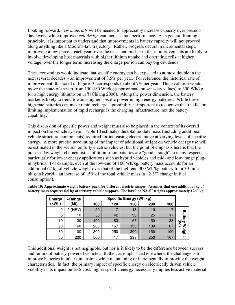
- 41 -

Looking forward, new materials will be needed to appreciably increase capacity over present-day levels, while improved cell design can increase rate performance. As a general framing principle, it is important to understand that improvements in battery capacity will not proceed along anything like a Moore’s-law trajectory. Rather, progress occurs in incremental steps, improving a few percent each year: over the near- and mid-term these improvements are likely to involve developing host materials with higher lithium uptake and operating cells at higher voltage; over the longer term, increasing the charge per ion can pay big dividends. These constraints would indicate that specific energy can be expected to at most double in the next several decades – an improvement of 3.5% per year. For reference, the historical rate of improvement illustrated in Figure 10 corresponds to about 7% per year. This evolution would move the state-of-the-art from 150-180 Wh/kg (approximate present-day values) to 300 Wh/kg for a high energy lithium-ion cell [Chiang 2006]. Along the power dimension, the battery market is likely to trend towards higher specific power in high energy batteries. While these high-rate batteries can make rapid recharge a possibility, it important to recognize that the factor limiting implementation of rapid recharge is the charging infrastructure, not the battery capability. This discussion of specific power and weight must also be placed in the context of its overall impact on the vehicle system. Table 10 estimates the total module mass (including additional vehicle structural components) required for increasing electric range at varying levels of specific energy. A more precise accounting of the impact of additional weight on vehicle energy use will be estimated in the section on fully electric-vehicles, but the point of emphasis here is that the present-day weight characteristics of lithium-ion batteries are “good enough” in many respects, particularly for lower energy applications such as hybrid vehicles and mid- and low- range plug-in hybrids. For example, even at the low-end of 100 Wh/kg, battery mass accounts for an additional 67 kg of vehicle weight over that of the high-end 300 Wh/kg battery for a 30-mile plug-in hybrid – an increase of ~5% of the total vehicle mass (a ~2-3% change in fuel consumption).

Table 10: Approximate weight battery pack for different electric ranges. Assumes that one additional kg of battery mass requires 0.5 kg of tertiary vehicle support. The baseline NA-SI weighs approximately 1260 kg.

Specific Energy (Wh/kg) Energy (kWh)

~Range (Mi) 100 120 150 200 300

2 0 (HEV) 20 17 13 10 7

5 10 50 42 33 25 17

10 30 100 83 67 50 33

20 60 200 167 133 100 67

30 100 300 250 200 150 100

50 200 500 417 333 250 167

Batte

ry W

eig

ht

(kg

)

This additional weight is not negligible, but nor is it likely to be the difference between success and failure of battery-powered vehicles. Rather, as emphasized elsewhere, the challenge is to improve batteries in other dimensions while maintaining or incrementally improving the weight characteristics. In fact, the primary impact of specific energy on electrically driven vehicle viability is its impact on ESS cost: higher specific energy necessarily implies less active material

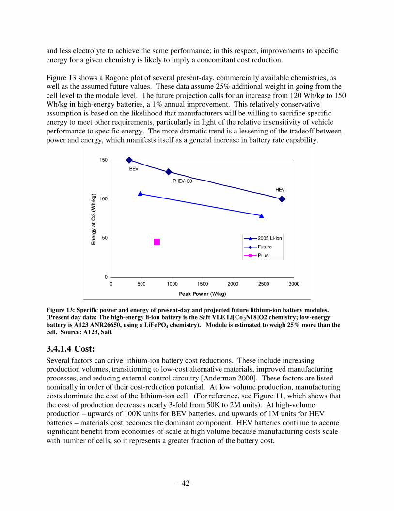
- 42 -

and less electrolyte to achieve the same performance; in this respect, improvements to specific energy for a given chemistry is likely to imply a concomitant cost reduction. Figure 13 shows a Ragone plot of several present-day, commercially available chemistries, as well as the assumed future values. These data assume 25% additional weight in going from the cell level to the module level. The future projection calls for an increase from 120 Wh/kg to 150 Wh/kg in high-energy batteries, a 1% annual improvement. This relatively conservative assumption is based on the likelihood that manufacturers will be willing to sacrifice specific energy to meet other requirements, particularly in light of the relative insensitivity of vehicle performance to specific energy. The more dramatic trend is a lessening of the tradeoff between power and energy, which manifests itself as a general increase in battery rate capability.

0

50

100

150

0 500 1000 1500 2000 2500 3000

Peak Power (W/kg)

En

erg

y a

t C

/3 (

Wh

/kg

)

2005 Li-Ion

Future

Prius

HEV

PHEV-30

BEV

Figure 13: Specific power and energy of present-day and projected future lithium-ion battery modules. (Present day data: The high-energy li-ion battery is the Saft VLE Li[Co.2Ni.8]O2 chemistry; low-energy battery is A123 ANR26650, using a LiFePO4 chemistry). Module is estimated to weigh 25% more than the cell. Source: A123, Saft

3.4.1.4 Cost:

Several factors can drive lithium-ion battery cost reductions. These include increasing production volumes, transitioning to low-cost alternative materials, improved manufacturing processes, and reducing external control circuitry [Anderman 2000]. These factors are listed nominally in order of their cost-reduction potential. At low volume production, manufacturing costs dominate the cost of the lithium-ion cell. (For reference, see Figure 11, which shows that the cost of production decreases nearly 3-fold from 50K to 2M units). At high-volume production – upwards of 100K units for BEV batteries, and upwards of 1M units for HEV batteries – materials cost becomes the dominant component. HEV batteries continue to accrue significant benefit from economies-of-scale at high volume because manufacturing costs scale with number of cells, so it represents a greater fraction of the battery cost.

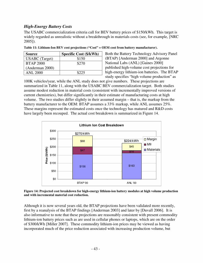
- 43 -

High-Energy Battery Costs

The USABC commercialization criteria call for BEV battery prices of $150/kWh. This target is widely regarded as unrealistic without a breakthrough in materials costs (see, for example, [NRC 2005]).

Table 11: Lithium-Ion BEV cost projections (“Cost” = OEM cost from battery manufacturer).

Both the Battery Technology Advisory Panel (BTAP) [Anderman 2000] and Argonne National Labs (ANL) [Gaines 2000] published high-volume cost projections for high-energy lithium-ion batteries. The BTAP study specifies “high volume production” as

100K vehicles/year, while the ANL study does not give numbers. These projections are summarized in Table 11, along with the USABC BEV commercialization target. Both studies assume modest reduction in material costs (consistent with incrementally improved versions of current chemistries), but differ significantly in their estimate of manufacturing costs at high volume. The two studies differ slightly in their assumed margin – that is, the markup from the battery manufacturer to the OEM: BTAP assumes a 33% markup, while ANL assumes 25%. These margins represent the estimated costs once the technology has matured and R&D costs have largely been recouped. The actual cost breakdown is summarized in Figure 14.

Lithium Ion Cost Breakdown

$156 $163

$47 $16

$68

$45

$0

$50

$100

$150

$200

$250

$300

BTAP '00 ANL '00

Pri

ce (

$/k

Wh

)

Margin

Mfr

Materials

$270/kWh

$224/kWh

Figure 14: Projected cost breakdown for high-energy lithium-ion battery modules at high volume production and with incremental material cost reduction.

Although it is now several years old, the BTAP projections have been validated more recently, first by a reanalysis of the BTAP findings [Anderman 2003] and later by [Duvall 2006]. It is also informative to note that these projections are reasonably consistent with present commodity lithium-ion battery prices such as are used in cellular phones or laptops, which are on the order of $300/kWh [Miller 2007]. These commodity lithium-ion prices may be viewed as having incorporated much of the price reduction associated with increasing production volume, but

Source Specific Cost ($/kWh) USABC (Target) $150

BTAP 2000 (Anderman 2000)

$270

ANL 2000 $225

- 44 -

without accounting for any transition to cheaper materials or additional costs associated with the safety and thermal control that automotive systems could require. This analysis indicates that the BTAP projection of $270/kWh continues to be a valid estimate for traditional high-energy lithium-ion chemistries in high-volume production. These estimates are generally based on lithium-ion cells using metal-oxide cathodes (nickel and manganese) and traditional high-cost electrolyte and separator materials for high-volume production in the 2010-2015 timeframe. Lower cost materials could drive further cost reductions. For example, one review showed that moving to iron-phosphate can reduce cathode costs from 50% to 10% of the total material cost [Ritchie 2006]. (At the same time, it is still an open question as to how well this particular chemistry will scale to high volume production). It should also be noted that the chemistry’s sensitivity to commodity metal prices could conceivably drive costs up. At the same time, because lithium-ion batteries can utilize a number of different materials, they should be well-positioned to adapt to long-term market trends. Over a 20 to 30 year timescale, a transition to lower cost materials that maintain favorable scale economies and low-cost manufacturing is well within the realm of possibility. Using the framework established by BTAP for estimating cost and applying the following assumptions yields a specific cost of ~$250/kWh.

Material costs from the BTAP baseline10 decrease by 40% over the next 20 years, a rate of 2.5% per year. This assumption is justified by the fact that improving specific energy should loosely translate into improved specific cost, as it implies that less active material is required to achieve a performance target. In section 3.4.1.3, it was assumed that specific energy improves at a rate of 3.5%/year over a 20 year period; however, because the battery must improve in other dimensions as well, a less aggressive 2.5% rate of improvement was chosen11.

Manufacturing costs and margins are unchanged from the BTAP projection In addition, an optimistic value of $200/kWh is used for sensitivity analysis in subsequent chapters. This cost is achievable with additional materials cost reduction and improvements to cell specific power.

High-Power Battery Costs

As discussed previously, traditional cell designs incur a tradeoff between energy and power; as such, higher power batteries such as those used in HEVs will tend to cost more on a per-kWh basis than the lower power batteries used in BEVs. However, as discussed above, the advent of low-cost nano-manufacturing processes could allow for high power batteries at high energy. Should this trend bear fruit, the cost per-kWh for HEV and plug-in hybrid batteries would likely drop. The total cost of the HEV packs could also be reduced with improved cycle life, which could allow more aggressive use of the available battery energy. A future HEV battery could meet the vehicle cycle life requirement while utilizing a wider state-of-charge envelope. This would enable a vehicle to be designed with a lower energy battery pack.

10 The BTAP projection shown in Figure 14 already includes a 30% reduction in cost of materials from their baseline. 11 Applying the 3.5% rate of improvement yields a specific cost of $210/kWh.

- 45 -

Over the long-term, the cost of these high-power batteries relative to high-energy batteries should drop dramatically. Mid-volume (100,000 packs/yr) year-2010 estimates project HEV lithium-ion batteries at $1000-$1500/kWh for a LiMn2O4 chemistry. A significant portion of this cost is related to pack integration/control and manufacturing costs [Anderman 2005]. Both of these factors could decrease significantly over time: the former due to more robust materials, and the latter due to high production volumes. The cost of a high-power lithium-ion pack (defined as a pack with a power-to-energy ratio of 35:1) is assumed to decrease to $750/kWh. As was the case for the energy battery, the projected cost falls short of the USABC target (in this case, $500/pack). At the same time, this shortfall is less daunting than in the case of the energy battery, first because the total dollar value is significantly lower, and second because, if energy storage is developed which can meet the cycle life requirements while operating over a wider charge envelope, the overall pack energy may be reduced. The optimistic case for the high-power battery assumes the same factor-3 difference between high-power and high-energy batteries; hence, with $200/kWh as the optimistic high-energy cost, the high-power battery would cost $600/kWh.

Cost as a Function of Rate Capability

To account for the varying power requirement along the continuum from the hybrid vehicle to various plug-in hybrid configurations to the battery-electric vehicle, the cost of increasing rate capability is treated as a linear function of the ratio of specific power to specific energy. Figure 15 shows this relationship for the different vehicles under consideration. This decreasing cost of high-power batteries is considered the key trend in lithium-ion battery performance.

Specific Cost ($/kWh)

0

200

400

600

800

1000

1200

1400

1600

0 5 10 15 20 25 30 35 40Power-to-Energy Ratio (W/Wh)

Current

Future Base Case

Future Optimistic

BEV

HEV

PHEV 30 PHEV 10

Figure 15: Current and future battery cost as a function of battery rate capability. Current data is based on a review of industry data and private correspondence [Miller 2007, Anderman 2000, Anderman 2005].

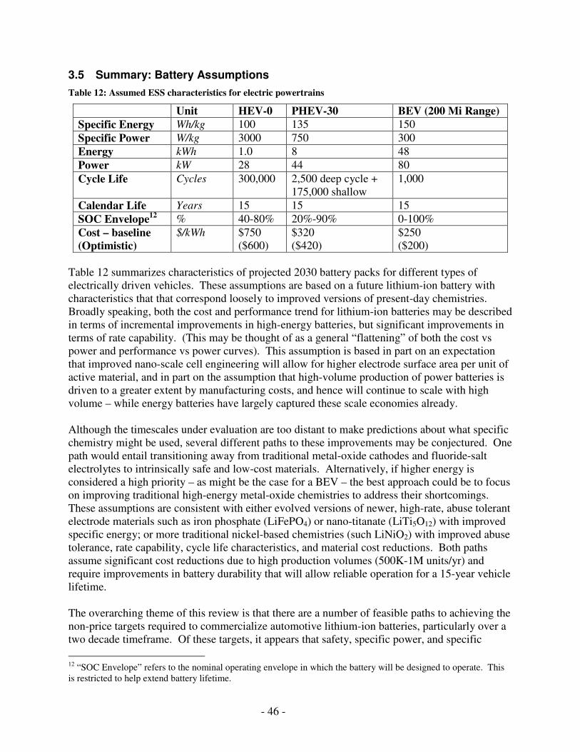
- 46 -

3.5 Summary: Battery Assumptions

Table 12: Assumed ESS characteristics for electric powertrains

Unit HEV-0 PHEV-30 BEV (200 Mi Range) Specific Energy Wh/kg 100 135 150

Specific Power W/kg 3000 750 300

Energy kWh 1.0 8 48

Power kW 28 44 80

Cycle Life Cycles 300,000 2,500 deep cycle + 175,000 shallow

1,000

Calendar Life Years 15 15 15

SOC Envelope12 % 40-80% 20%-90% 0-100%

Cost – baseline (Optimistic)

$/kWh $750 ($600)

$320 ($420)

$250 ($200)

Table 12 summarizes characteristics of projected 2030 battery packs for different types of electrically driven vehicles. These assumptions are based on a future lithium-ion battery with characteristics that that correspond loosely to improved versions of present-day chemistries. Broadly speaking, both the cost and performance trend for lithium-ion batteries may be described in terms of incremental improvements in high-energy batteries, but significant improvements in terms of rate capability. (This may be thought of as a general “flattening” of both the cost vs power and performance vs power curves). This assumption is based in part on an expectation that improved nano-scale cell engineering will allow for higher electrode surface area per unit of active material, and in part on the assumption that high-volume production of power batteries is driven to a greater extent by manufacturing costs, and hence will continue to scale with high volume – while energy batteries have largely captured these scale economies already. Although the timescales under evaluation are too distant to make predictions about what specific chemistry might be used, several different paths to these improvements may be conjectured. One path would entail transitioning away from traditional metal-oxide cathodes and fluoride-salt electrolytes to intrinsically safe and low-cost materials. Alternatively, if higher energy is considered a high priority – as might be the case for a BEV – the best approach could be to focus on improving traditional high-energy metal-oxide chemistries to address their shortcomings. These assumptions are consistent with either evolved versions of newer, high-rate, abuse tolerant electrode materials such as iron phosphate (LiFePO4) or nano-titanate (LiTi5O12) with improved specific energy; or more traditional nickel-based chemistries (such LiNiO2) with improved abuse tolerance, rate capability, cycle life characteristics, and material cost reductions. Both paths assume significant cost reductions due to high production volumes (500K-1M units/yr) and require improvements in battery durability that will allow reliable operation for a 15-year vehicle lifetime. The overarching theme of this review is that there are a number of feasible paths to achieving the non-price targets required to commercialize automotive lithium-ion batteries, particularly over a two decade timeframe. Of these targets, it appears that safety, specific power, and specific

12 “SOC Envelope” refers to the nominal operating envelope in which the battery will be designed to operate. This is restricted to help extend battery lifetime.

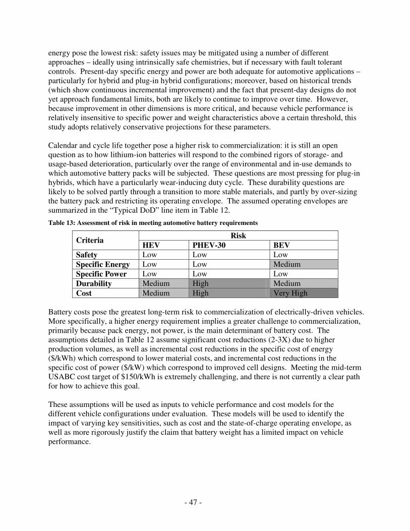
- 47 -

energy pose the lowest risk: safety issues may be mitigated using a number of different approaches – ideally using intrinsically safe chemistries, but if necessary with fault tolerant controls. Present-day specific energy and power are both adequate for automotive applications – particularly for hybrid and plug-in hybrid configurations; moreover, based on historical trends (which show continuous incremental improvement) and the fact that present-day designs do not yet approach fundamental limits, both are likely to continue to improve over time. However, because improvement in other dimensions is more critical, and because vehicle performance is relatively insensitive to specific power and weight characteristics above a certain threshold, this study adopts relatively conservative projections for these parameters. Calendar and cycle life together pose a higher risk to commercialization: it is still an open question as to how lithium-ion batteries will respond to the combined rigors of storage- and usage-based deterioration, particularly over the range of environmental and in-use demands to which automotive battery packs will be subjected. These questions are most pressing for plug-in hybrids, which have a particularly wear-inducing duty cycle. These durability questions are likely to be solved partly through a transition to more stable materials, and partly by over-sizing the battery pack and restricting its operating envelope. The assumed operating envelopes are summarized in the “Typical DoD” line item in Table 12.

Table 13: Assessment of risk in meeting automotive battery requirements

Risk Criteria

HEV PHEV-30 BEV Safety Low Low Low

Specific Energy Low Low Medium

Specific Power Low Low Low

Durability Medium High Medium

Cost Medium High Very High

Battery costs pose the greatest long-term risk to commercialization of electrically-driven vehicles. More specifically, a higher energy requirement implies a greater challenge to commercialization, primarily because pack energy, not power, is the main determinant of battery cost. The assumptions detailed in Table 12 assume significant cost reductions (2-3X) due to higher production volumes, as well as incremental cost reductions in the specific cost of energy ($/kWh) which correspond to lower material costs, and incremental cost reductions in the specific cost of power ($/kW) which correspond to improved cell designs. Meeting the mid-term USABC cost target of $150/kWh is extremely challenging, and there is not currently a clear path for how to achieve this goal. These assumptions will be used as inputs to vehicle performance and cost models for the different vehicle configurations under evaluation. These models will be used to identify the impact of varying key sensitivities, such as cost and the state-of-charge operating envelope, as well as more rigorously justify the claim that battery weight has a limited impact on vehicle performance.

- 48 -

4 Spark-Ignition Engines, Diesels, and Hybrids

Kasseris 2006 undertook a detailed analysis of the naturally-aspirated spark ignition (NA-SI) engine, a turbo-charged spark ignition (turbo SI) engine, a diesel, and a hybrid-electric vehicle (HEV). This previous study uses the same methodology and assumptions that are used for modeling vehicles in the current study. The fuel consumption results of the Kasseris work for the 2.5L Toyota Camry are shown in Table 14; these are presented for comparison purposes with the new technologies that are evaluated in this study (see Appendix 2: Fuel Consumption & Energy Use for complete results for all vehicle technologies).

Table 14: Fuel Consumption Results from [Kasseris 2006] for the 2.5L Camry

Units

2006 NA-SI

NA-SI Turbo Diesel HEV

FTP, Unadjusted L/100 km 8.9 5.7 5.0 4.9 2.5

HWFET, Unadjusted L/100 km 5.9 3.5 3.1 3.0 2.7

US06 L/100 km 8.3 5.4 5.0 4.9 4.0

Combined, Adjusted L/100 km 8.84 5.49 4.73 4.73 3.07

Industry L/100 km 7.70 4.87 4.27 4.37 3.07

GHG Emissions (Comb, Adj)

g CO2/km 244 151 134 128 88

The current study builds on the results of the previous assessment, particularly with respect to the hybrid. First, several revisions to the previous hybrid model are presented for consistency with other projections detailed in this study. Then, several special considerations related to deployment of hybrid vehicles are addressed. The chapter closes by developing cost estimates for technologies.

4.1 Key Assumptions about the Hybrid Vehicle

Because the hybrid vehicle is an important piece of the current study, the key assumptions from the previous hybrid projection are reviewed below. A hybrid vehicle can improve vehicle efficiency in a number of different ways:

1.) It can turn the engine off during idle 2.) It can recapture the vehicle’s kinetic energy using regenerative braking 3.) It minimizes the amount of time the engine operates under low-efficiency partial-load

conditions. This engine optimization may be achieved in a number of ways: a. Down-sized engine: Because the hybrid substitutes engine power with motor

power, it enables a down-sized engine. A smaller engine spends more of its time operating in the high-efficiency, high load regime.

b. Active engine optimization: A hybrid vehicle may use its limited energy storage capacity and small motor to turn the engine off during periods of low-efficiency operation (low-speed, low-torque conditions); alternatively, a hybrid can also shunt engine power into the battery, thereby boosting the engine load into the high efficiency regime. A similar benefit may be achieved with a high-efficiency mechanical continuously variable transmission (CVT).

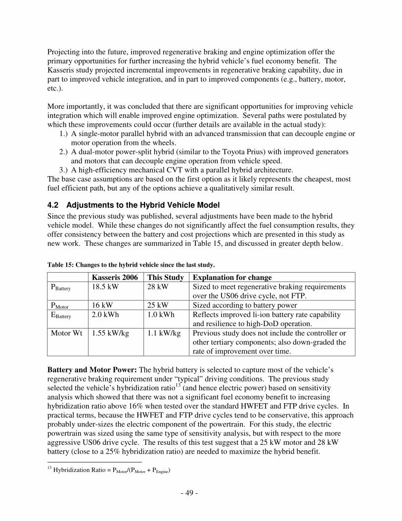
- 49 -

Projecting into the future, improved regenerative braking and engine optimization offer the primary opportunities for further increasing the hybrid vehicle’s fuel economy benefit. The Kasseris study projected incremental improvements in regenerative braking capability, due in part to improved vehicle integration, and in part to improved components (e.g., battery, motor, etc.). More importantly, it was concluded that there are significant opportunities for improving vehicle integration which will enable improved engine optimization. Several paths were postulated by which these improvements could occur (further details are available in the actual study):

1.) A single-motor parallel hybrid with an advanced transmission that can decouple engine or motor operation from the wheels.

2.) A dual-motor power-split hybrid (similar to the Toyota Prius) with improved generators and motors that can decouple engine operation from vehicle speed.

3.) A high-efficiency mechanical CVT with a parallel hybrid architecture. The base case assumptions are based on the first option as it likely represents the cheapest, most fuel efficient path, but any of the options achieve a qualitatively similar result.

4.2 Adjustments to the Hybrid Vehicle Model

Since the previous study was published, several adjustments have been made to the hybrid vehicle model. While these changes do not significantly affect the fuel consumption results, they offer consistency between the battery and cost projections which are presented in this study as new work. These changes are summarized in Table 15, and discussed in greater depth below.

Table 15: Changes to the hybrid vehicle since the last study.

Kasseris 2006 This Study Explanation for change PBattery 18.5 kW 28 kW Sized to meet regenerative braking requirements

over the US06 drive cycle, not FTP.

PMotor 16 kW 25 kW Sized according to battery power

EBattery 2.0 kWh 1.0 kWh Reflects improved li-ion battery rate capability and resilience to high-DoD operation.

Motor Wt 1.55 kW/kg 1.1 kW/kg Previous study does not include the controller or other tertiary components; also down-graded the rate of improvement over time.

Battery and Motor Power: The hybrid battery is selected to capture most of the vehicle’s regenerative braking requirement under “typical” driving conditions. The previous study selected the vehicle’s hybridization ratio13 (and hence electric power) based on sensitivity analysis which showed that there was not a significant fuel economy benefit to increasing hybridization ratio above 16% when tested over the standard HWFET and FTP drive cycles. In practical terms, because the HWFET and FTP drive cycles tend to be conservative, this approach probably under-sizes the electric component of the powertrain. For this study, the electric powertrain was sized using the same type of sensitivity analysis, but with respect to the more aggressive US06 drive cycle. The results of this test suggest that a 25 kW motor and 28 kW battery (close to a 25% hybridization ratio) are needed to maximize the hybrid benefit.

13 Hybridization Ratio = PMotor/(PMotor + PEngine)

- 50 -

Battery Energy: Based on further review of lithium-ion technology and the hybrid battery energy requirements, it was concluded that a future hybrid vehicle is likely to require less battery energy than was assumed previously. This conclusion is based on two important trends in battery development: the first is that lithium-ion chemistries currently coming to market offer a higher power-to-energy ratio than was assumed in the initial assessment. It is assumed that this trend towards higher power and higher reliability will continue. The second factor is that improved cell design will enable hybrid batteries to operate over a wider state-of-charge envelope without degrading the battery performance or life. The Generation 2 Toyota Prius is rated at 1.3 kWh; in practical terms, this battery has a useable energy on the order of 600 Wh [Miller 2007, Muta 2004]. This restriction exists both because battery rate capability (i.e., its power output) degrades at high depth-of-discharge, and because battery cycle-life degradation correlates with depth-of-discharge. These constraints may both become less stringent with continued development. It should also be stressed that, under normal driving conditions, the actual battery operating envelope is significantly narrower than the 600 Wh maximum; as a point of reference, the aggressive US06 drive cycle operates over a 10% state-of-charge window. The extra energy adds robustness for conditions such as hill climbing and low-speed electric operation. To account for continuing technological developments which would allow for higher power, lower energy hybrid batteries, the future lithium-ion battery is assumed to deliver the required 28 kW of power with a battery that is rated at 1 kWh (20% less energy than that of the present-day Prius). As mentioned previously, the adjustments to the hybrid vehicle model do not impact the fuel consumption results; however, these assumptions carry over to other vehicle technologies for which judgments about battery and motor weight are more sensitive. They also impact the hybrid vehicle cost projections.

4.3 Special Considerations

Present-day hybrids are often characterized as having a less robust fuel consumption benefit relative to diesel and spark-ignition powertrains than their EPA-rated fuel efficiency would indicate. Specifically, two important questions that are often raised:

1.) Does the hybrid vehicle continue to offer fuel consumption benefits during aggressive, high-speed drive cycles?

2.) Does the hybrid suffer a disproportionately high fuel-consumption penalty due to high accessory loads (such as air conditioning)?

These questions are important when extrapolating the hybrid vehicle results to the fleet as a whole. If these effects are significant then it would suggest that different test cycles be used to measure hybrid vehicle fuel consumption14. There are several reasons why a hybrid vehicle’s fuel economy benefit under aggressive, high speed driving conditions would decrease: engine operation is already fairly well optimized at

14 Alternatively, different adjustment factors could be applied to the EPA-standard 0.9 FTP/0.78 HWFET.

- 51 -

high speed operation; there is limited time at idle; proportionately less vehicle energy is used for braking, and hence cannot be recaptured via the regenerative path; and braking at high speeds can overwhelm the regenerative capture capability of the battery – meaning that some power is dissipated through conventional friction braking. In addition to these factors, a present day hybrid vehicle weighs more than a non-hybrid equivalent (~40 kg for a Honda Civic, up to ~150 kg for an SUV like the Ford Escape [autos.com]).

2030 Hybrid Energy Flows 2030 NA-SI Energy Flows

Figure 16: Energy flows over the different drive cycles (Left: HEV; Right: 2030 NA-SI)

US06 Cycle

FTP Cycle

HWFET Cycle

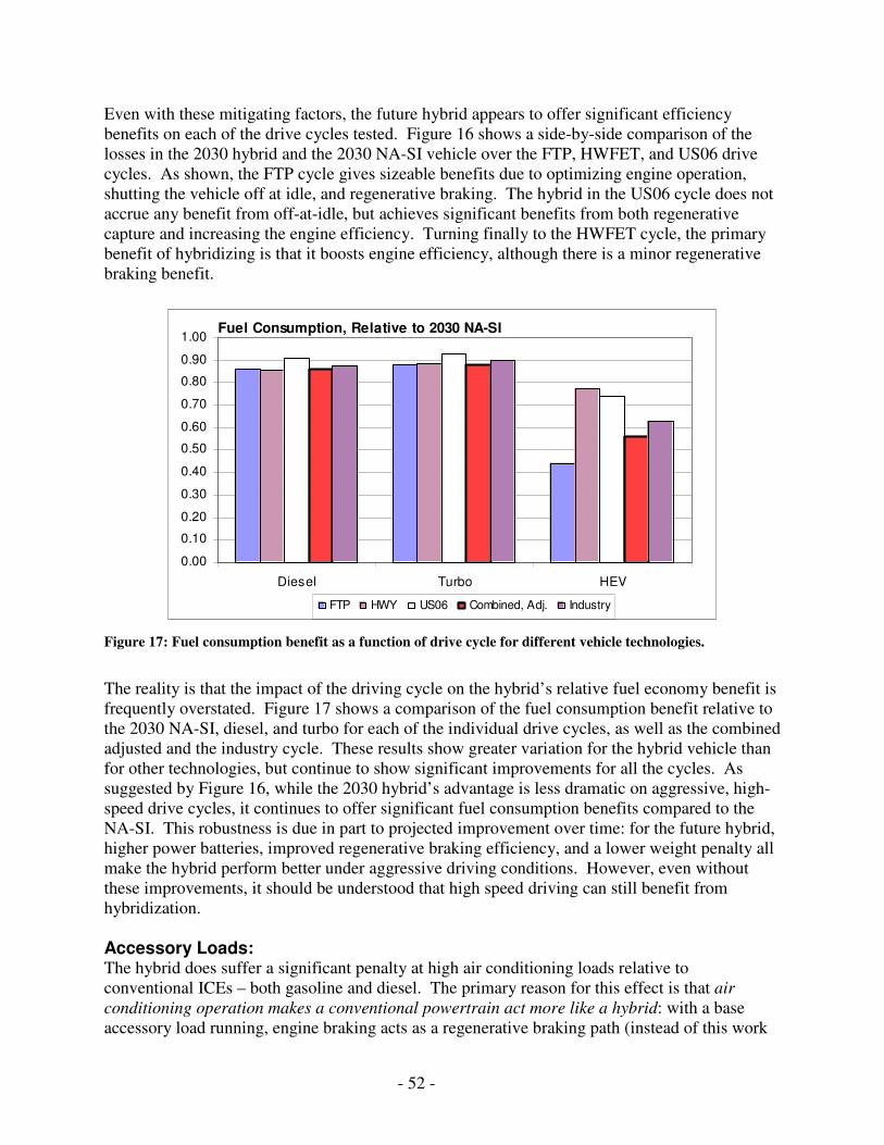
- 52 -

Even with these mitigating factors, the future hybrid appears to offer significant efficiency benefits on each of the drive cycles tested. Figure 16 shows a side-by-side comparison of the losses in the 2030 hybrid and the 2030 NA-SI vehicle over the FTP, HWFET, and US06 drive cycles. As shown, the FTP cycle gives sizeable benefits due to optimizing engine operation, shutting the vehicle off at idle, and regenerative braking. The hybrid in the US06 cycle does not accrue any benefit from off-at-idle, but achieves significant benefits from both regenerative capture and increasing the engine efficiency. Turning finally to the HWFET cycle, the primary benefit of hybridizing is that it boosts engine efficiency, although there is a minor regenerative braking benefit.

Fuel Consumption, Relative to 2030 NA-SI

0.00

0.10

0.20

0.30

0.40

0.50

0.60

0.70

0.80

0.90

1.00

Diesel Turbo HEV

FTP HWY US06 Combined, Adj. Industry

Figure 17: Fuel consumption benefit as a function of drive cycle for different vehicle technologies.

The reality is that the impact of the driving cycle on the hybrid’s relative fuel economy benefit is frequently overstated. Figure 17 shows a comparison of the fuel consumption benefit relative to the 2030 NA-SI, diesel, and turbo for each of the individual drive cycles, as well as the combined adjusted and the industry cycle. These results show greater variation for the hybrid vehicle than for other technologies, but continue to show significant improvements for all the cycles. As suggested by Figure 16, while the 2030 hybrid’s advantage is less dramatic on aggressive, high-speed drive cycles, it continues to offer significant fuel consumption benefits compared to the NA-SI. This robustness is due in part to projected improvement over time: for the future hybrid, higher power batteries, improved regenerative braking efficiency, and a lower weight penalty all make the hybrid perform better under aggressive driving conditions. However, even without these improvements, it should be understood that high speed driving can still benefit from hybridization. Accessory Loads: The hybrid does suffer a significant penalty at high air conditioning loads relative to conventional ICEs – both gasoline and diesel. The primary reason for this effect is that air conditioning operation makes a conventional powertrain act more like a hybrid: with a base accessory load running, engine braking acts as a regenerative braking path (instead of this work

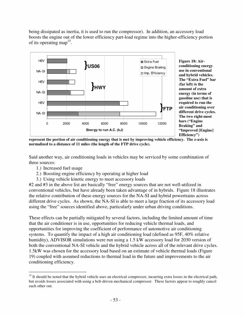
- 53 -

0 2000 4000 6000 8000 10000 12000

NA-SI

HEV

NA-SI

HEV

NA-SI

HEV

Energy to run A.C. (kJ)

Extra Fuel

Engine Braking

Imp. Eff iciency

US06

HWY

FTP

being dissipated as inertia, it is used to run the compressor). In addition, an accessory load boosts the engine out of the lower efficiency part-load regime into the higher-efficiency portion of its operating map15.

Figure 18: Air-conditioning energy use in conventional and hybrid vehicles. The “Extra Fuel” bar (far left) is the amount of extra energy (in terms of gasoline use) that is required to run the air conditioning over different drive cycles. The two right-most bars (“Engine Braking” and “Improved [Engine] Efficiency”)

represent the portion of air conditioning energy that is met by improving vehicle efficiency. The z-axis is normalized to a distance of 11 miles (the length of the FTP drive cycle).

Said another way, air conditioning loads in vehicles may be serviced by some combination of three sources:

1.) Increased fuel usage 2.) Boosting engine efficiency by operating at higher load 3.) Using vehicle kinetic energy to meet accessory loads

#2 and #3 in the above list are basically “free” energy sources that are not well-utilized in conventional vehicles, but have already been taken advantage of in hybrids. Figure 18 illustrates the relative contribution of these energy sources for the NA-SI and hybrid powertrains across different drive cycles. As shown, the NA-SI is able to meet a large fraction of its accessory load using the “free” sources identified above, particularly under urban driving conditions. These effects can be partially mitigated by several factors, including the limited amount of time that the air conditioner is in use, opportunities for reducing vehicle thermal loads, and opportunities for improving the coefficient of performance of automotive air conditioning systems. To quantify the impact of a high air conditioning load (defined as 95F, 40% relative humidity), ADVISOR simulations were run using a 1.5 kW accessory load for 2030 version of both the conventional NA-SI vehicle and the hybrid vehicle across all of the relevant drive cycles. 1.5kW was chosen for the accessory load based on an estimate of vehicle thermal loads (Figure 19) coupled with assumed reductions to thermal load in the future and improvements to the air conditioning efficiency.

15 It should be noted that the hybrid vehicle uses an electrical compressor, incurring extra losses in the electrical path, but avoids losses associated with using a belt-driven mechanical compressor. These factors appear to roughly cancel each other out.

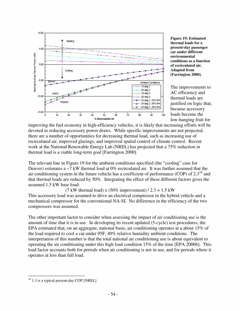
- 54 -

Figure 19: Estimated thermal loads for a present-day passenger car under different environmental conditions as a function of recirculated air. Adapted from [Farrington 2000].

The improvements to AC efficiency and thermal loads are justified on logic that, because accessory loads become the low-hanging fruit for

improving the fuel economy in high-efficiency vehicles, it is likely that increasing efforts will be devoted to reducing accessory power draws. While specific improvements are not projected, there are a number of opportunities for decreasing thermal load, such as increasing use of recirculated air, improved glazings, and improved spatial control of climate control. Recent work at the National Renewable Energy Lab (NREL) has projected that a 75% reduction in thermal load is a viable long-term goal [Farrington 2000]. The relevant line in Figure 19 for the ambient conditions specified (the “cooling” case for Denver) estimates a ~7 kW thermal load at 0% recirculated air. It was further assumed that the air conditioning system in the future vehicle has a coefficient of performance (COP) of 2.316 and that thermal loads are reduced by 50%. Integrating the effect of these different factors gives the assumed 1.5 kW base load:

(7 kW thermal load) x (50% improvement) / 2.3 = 1.5 kW This accessory load was assumed to drive an electrical compressor in the hybrid vehicle and a mechanical compressor for the conventional NA-SI. No difference in the efficiency of the two compressors was assumed. The other important factor to consider when assessing the impact of air conditioning use is the amount of time that it is in use. In developing its recent updated (5-cycle) test procedures, the EPA estimated that, on an aggregate, national basis, air conditioning operates at a about 15% of the load required to cool a car under 95F, 40% relative humidity ambient conditions. The interpretation of this number is that the total national air conditioning use is about equivalent to operating the air conditioning under this high load condition 15% of the time [EPA 2006b]. This load factor accounts both for periods when air conditioning is not in use, and for periods where it operates at less than full load.

16 1.3 is a typical present-day COP [NREL]

- 55 -

Figure 20 shows the impact of air conditioning use on the hybrid vehicle relative to the NA-SI. The first bar shows the relative fuel consumption with no accessory load; the middle bar shows the impact of running the air conditioning at full load all the time; and the third bar shows the weighted impact (using the EPA estimate of 15% AC / 85% No AC). The results show a significant impact over the FTP drive cycle, where the NA-SI benefits the most from engine braking and raising the efficiency, but a relatively minor effect on the US06 and HWFET drive cycles. Over the combined and industry cycles, the impact of the FTP cycle is damped considerably.

HEV Fuel Consumption, Relative to the 2030 NA-SI

0.00

0.20

0.40

0.60

0.80

1.00

FTP HWY US06 Comb Ind

No Air Conditioning

1.5 kW AC Load

Weighted Impact of AC

Figure 20: Impact of air conditioning loads on hybrid vehicle fuel consumption

Perhaps more importantly, the aggregate impact of air conditioning load is relatively small due to the limited time-in-use. The results for both the combined cycle and the industry cycle show a fuel consumption impact on the order of 3%. However, the impact of air conditioning use during hot weather, particularly in urban driving conditions is significant. While in the aggregate this may be a small fraction of vehicle-miles, it suggests that the benefits of the hybrid vehicle are reduced for parts of the country for which these conditions are the norm (such as Miami, New Orleans, or Phoenix). Summary: The results of the sensitivity analysis suggest that the future hybrid will be more robust to varying driving patterns than current hybrids are given credit for. While the fuel consumption benefit of the hybrid is lower over the highway and US06 drive cycle, it is still significant. In a similar vein, under environmental extremes, the hybrid will suffer a disproportionate penalty due to high accessory loads. However, in the aggregate, accounting for different drive cycles and climatic variation, this effect is relatively minor. The other important implication of this analysis is that the hybrid vehicle is not equally appropriate for all consumers: an individual living in a humid climate or who drives a disproportionate amount of the time on the highway might do better in an advanced diesel. On the other side, the hybrid can deliver an increased advantage to an individual living in a moderate climate with a predominantly urban driving pattern.

- 56 -

4.4 Cost Projections for NA-SI, Turbo, Diesel, and Hybrid Vehicles

Costs for the mainstream, mature technologies under evaluation – the spark-ignition engine, the turbo, and the diesel – are drawn primarily from the 2006 Concawe well-to-wheel study [Concawe 2006], conversations within industry, and [Weiss 2000]. For reference, a comprehensive list of all the cost assumptions for all the vehicle technologies, as well as relevant sources, is included in Section 8.2. The costs of the mainstream technologies are projected to increase from present-day values due to improving technology and evolving emissions constraints. While no specific assumptions were made about which specific improvements to the 2030 NA-SI vehicle would offer the projected efficiency gains, for cost purposes, it is assumed that the vehicle uses a gasoline direct-inject (GDI) with variable valve timing and lift (VVLT) and other built-in improvements (such as weight reduction) at a projected incremental cost of $700 more than the present day NA-SI. The turbo-charged gasoline engine is assumed to require these improvements, plus a turbocharger, at a projected incremental cost of $500 relative to the 2030 baseline. In addition, all of the spark-ignition engines (including the hybrid and the plug-in hybrid) are assumed to require exhaust after-treatment costing $300. The incremental cost of the diesel compared to the spark-ignition vehicle includes additional costs for the engine and for exhaust after-treatments. The cost of a diesel engine compared to a present-day spark-ignition engine is widely quoted as $1,400; however. This means that the gap in engine price narrows to $700 once the cost of new spark-ignition technology is incorporated. The exhaust after-treatment includes a diesel particulate filter and a to-be-determined NOx catalyst – estimated to cost $800 in the long-term ($500 more than the 2030 NA-SI). Summing the engine and after-treatment costs gives an incremental cost for the diesel of $1,200.

Table 16: Estimated current and future hybrid vehicle incremental costs. For assumptions about the future hybrid vehicle cost, see Table 51 and Table 52.

Incremental Current HEV Cost, compared to 2006 NA-SI

Incremental Future HEV cost, compared to 2030 NA-SI

Architecture: Single-Motor17 (e.g., Honda)

Power Split18 (e.g., Toyota)

Single-motor w/advanced transmission

Motor $800 (25 kW) $1,300 (50 kW) $600 (25 kW)

Generator - $600 (15 kW) --

Battery $1,600 (1.3 kWh) $1,600 (1.3 kWh) $900 (1 kWh)

Wiring $200 $200 $200

Transmission -- -$200 (Planetary Gear) $300

Engine Credit -$100 -$100 -$100

Total $2,500 $3,400 $1,900

The hybrid vehicle has a significant opportunity to decrease costs over those of present-day hybrids. The incremental cost of a hybrid vehicle is primarily a function of the battery and motor/controller costs, although additional smaller adjustments are made for factors such as differences in transmission, wiring, and the downsized engine. Table 16 shows a breakdown of n estimated hybrid vehicle costs for two different present-day hybrid architectures, and the

17 Current single-motor HEV cost assumptions: Battery: 1.25 kWh @ $1,200/kWh; Motor: $20/kW + $300 18 Same assumptions as for single-motor.

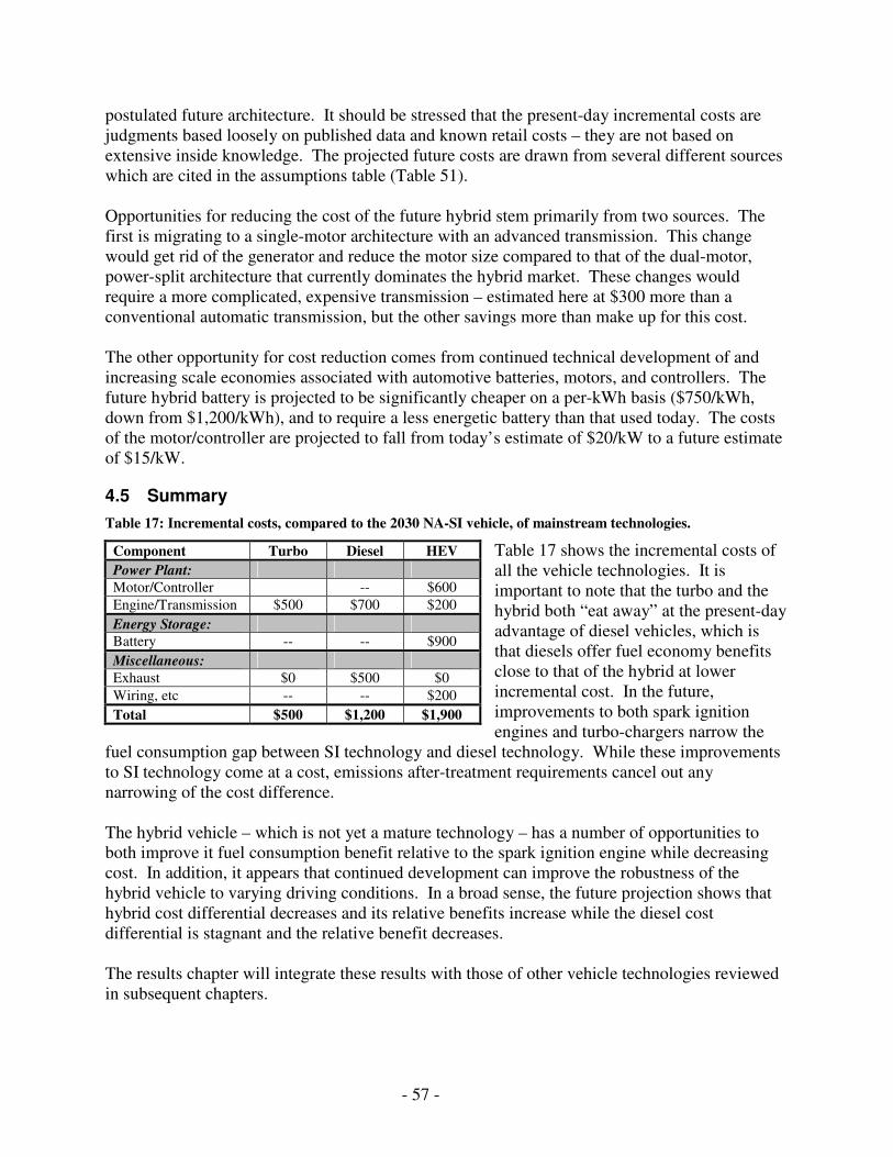
- 57 -

postulated future architecture. It should be stressed that the present-day incremental costs are judgments based loosely on published data and known retail costs – they are not based on extensive inside knowledge. The projected future costs are drawn from several different sources which are cited in the assumptions table (Table 51). Opportunities for reducing the cost of the future hybrid stem primarily from two sources. The first is migrating to a single-motor architecture with an advanced transmission. This change would get rid of the generator and reduce the motor size compared to that of the dual-motor, power-split architecture that currently dominates the hybrid market. These changes would require a more complicated, expensive transmission – estimated here at $300 more than a conventional automatic transmission, but the other savings more than make up for this cost. The other opportunity for cost reduction comes from continued technical development of and increasing scale economies associated with automotive batteries, motors, and controllers. The future hybrid battery is projected to be significantly cheaper on a per-kWh basis ($750/kWh, down from $1,200/kWh), and to require a less energetic battery than that used today. The costs of the motor/controller are projected to fall from today’s estimate of $20/kW to a future estimate of $15/kW.

4.5 Summary

Table 17: Incremental costs, compared to the 2030 NA-SI vehicle, of mainstream technologies.

Table 17 shows the incremental costs of all the vehicle technologies. It is important to note that the turbo and the hybrid both “eat away” at the present-day advantage of diesel vehicles, which is that diesels offer fuel economy benefits close to that of the hybrid at lower incremental cost. In the future, improvements to both spark ignition engines and turbo-chargers narrow the

fuel consumption gap between SI technology and diesel technology. While these improvements to SI technology come at a cost, emissions after-treatment requirements cancel out any narrowing of the cost difference. The hybrid vehicle – which is not yet a mature technology – has a number of opportunities to both improve it fuel consumption benefit relative to the spark ignition engine while decreasing cost. In addition, it appears that continued development can improve the robustness of the hybrid vehicle to varying driving conditions. In a broad sense, the future projection shows that hybrid cost differential decreases and its relative benefits increase while the diesel cost differential is stagnant and the relative benefit decreases. The results chapter will integrate these results with those of other vehicle technologies reviewed in subsequent chapters.

Component Turbo Diesel HEV

Power Plant:

Motor/Controller -- $600

Engine/Transmission $500 $700 $200

Energy Storage:

Battery -- -- $900

Miscellaneous:

Exhaust $0 $500 $0

Wiring, etc -- -- $200

Total $500 $1,200 $1,900

- 58 -

5 Plug-In Hybrid-Electric Vehicles

5.1 Overview

This chapter will assess the tank-to-wheels energy and petroleum consumption of the plug-in hybrid; cost, technological, and infrastructure-related implementation challenges will also be discussed. Finally, the results of the tank-to-wheel vehicle assessment will be integrated with the well-to-tank estimate of electric grid emissions and energy use. Several developments in the last several years have heightened interest in the plug-in hybrid. These drivers include the apparent success of hybrids in the marketplace, which may indicate that there is a market premium for “green” advanced vehicles; advances in lithium-ion battery technology, which might enable vehicles with limited electric range to come to a mass-market; high fuel prices and environmental concerns, which may provide a greater market pull; and daunting obstacles presented by transitioning to “ultimate” sustainability solutions, such as BEVs or fuel-cells, which may indicate that their time-to-market lies on too great of a time horizon to provide meaningful contributions in the next several decades. Because the plug-in hybrid has only recently warranted serious discussion and presents such a radical departure from vehicles available today, data is sparse as to how vehicles should be configured, how energy should be accounted between dual-operating modes, and what design points make sense. It is also not clear how to determine upstream energy use from electricity; nor is it clear what implementation issues may manifest themselves. To resolve these issues, this chapter will proceed as follows:

1.) Define a methodology for assessing vehicle energy use; 2.) Identify reasonable design points with respect to vehicle range, platform, and control

strategy. 3.) Identify implementation challenges presented by a mass-market plug-in hybrid and

mitigation strategies for addressing these issues. 4.) Present data on energy use and cost for future plug-ins.

It should be noted that the key technological challenge to deploying plug-in hybrids relates to battery performance. These issues are discussed in detail in Chapter 3. In addition, vehicle-to-grid technology is a promising possibility, but is not included in the scope of this study.

5.2 Plug-in Hybrid Defined

Figure 21: PHEV operating modes.

A plug-in hybrid-electric vehicle (PHEV) is a hybrid-vehicle with the ability to recharge from the grid. It is endowed with a modest electric driving range (on the order of tens of miles), and a small gasoline-powered ICE. The

PHEV offers a compromise between the drivability and affordability of the hybrid-electric vehicle (HEV), and the potential environmental and energy security benefits of the battery-

- 59 -

electric vehicle (BEV). Like the BEV, the PHEV possesses the capability to displace petroleum-sourced energy with grid-sourced energy; and, like the HEV, the PHEV is not range limited in any meaningful sense. Above a threshold minimum battery state-of-charge, the PHEV operates in “charge depleting” mode, in which it freely draws down the onboard battery to meet vehicle power demands. Once it reaches this minimum SOC threshold, the vehicle switches to “charge sustaining” mode (Figure 21). Charge-sustaining mode is functionally equivalent to vehicle operation in a conventional HEV. During this mode of operation, the vehicle maintains the SOC within a limited operating envelope (the overall SOC excursion during this mode of operation might be on the order of +/- 200 W-hr), using stored battery energy to optimize ICE operation, and recharging via either regenerative braking or an accessory-like loading on the engine.

5.3 Methodology

5.4 Vehicle Design Constraints

To maintain consistency with other vehicles comparisons, the following vehicle performance characteristics are used to constrain the PHEV design:

1.) In keeping with our notion of ‘equivalent performance’ between different powertrains, the vehicle should be capable of accelerating from 0-60 in about 9.3 seconds.

2.) The vehicle must provide adequate motive power to meet the US06 drive cycle in both charge-sustaining and charge-depleting modes.

3.) The vehicle must meet a minimum grade requirement of 55 MPH on a 6% grade19. For the grade climbing evaluation, vehicles are assumed to operate only under engine power, as a sustained hill climb will quickly deplete battery power and offer no opportunity for recharging the battery via regenerative braking.

4.) The electrical powertrain must be powerful enough to optimize engine operation during charge-sustaining operation, and recapture a majority of vehicle kinetic energy through regenerative braking during the US06 drive cycle.

In practice, the US06 requirement presents the most stringent constraint on vehicle configuration. Within these constraints, the design should optimize between vehicle cost and utility. Hence, designs will converge on the smallest electrical powertrain that can meet these requirements without significantly impacting the incremental energy/fuel savings.

5.4.1 Electric Range

For a variety of reasons, the “electric range” of a plug-in hybrid vehicle is a loosely defined concept: first, electric range depends greatly on assumptions about the drive cycle and how much battery energy is actually useable. In addition, depending on the design strategy adopted, the vehicle may use a smaller electric powertrain supplemented by the engine during charge-depleting mode – thereby extending the charge-depleting range. For this evaluation, the electric range is defined as the distance the vehicle travels using electric power over the industry cycle (an average of the HWFET, FTP, and US06 drive cycles), which is close to that of the combined-adjusted cycle – about 190-200 Wh/mi, depending on the vehicle

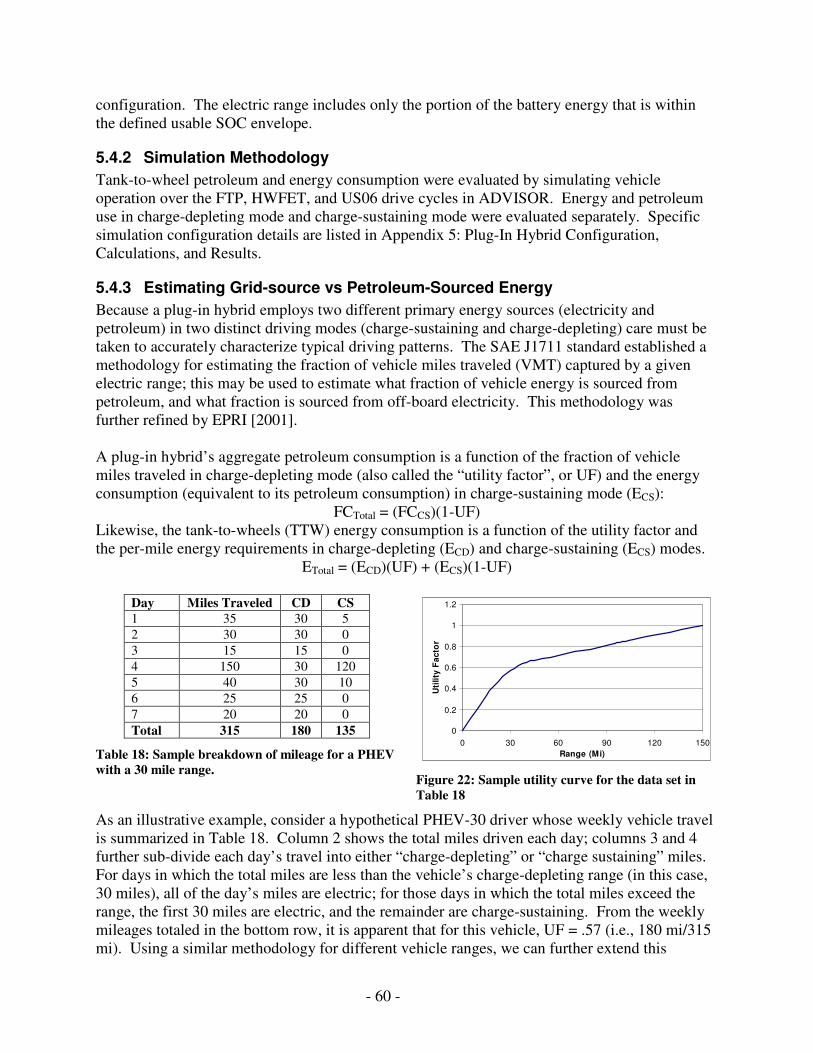
- 60 -

configuration. The electric range includes only the portion of the battery energy that is within the defined usable SOC envelope.

5.4.2 Simulation Methodology

Tank-to-wheel petroleum and energy consumption were evaluated by simulating vehicle operation over the FTP, HWFET, and US06 drive cycles in ADVISOR. Energy and petroleum use in charge-depleting mode and charge-sustaining mode were evaluated separately. Specific simulation configuration details are listed in Appendix 5: Plug-In Hybrid Configuration, Calculations, and Results.

5.4.3 Estimating Grid-source vs Petroleum-Sourced Energy

Because a plug-in hybrid employs two different primary energy sources (electricity and petroleum) in two distinct driving modes (charge-sustaining and charge-depleting) care must be taken to accurately characterize typical driving patterns. The SAE J1711 standard established a methodology for estimating the fraction of vehicle miles traveled (VMT) captured by a given electric range; this may be used to estimate what fraction of vehicle energy is sourced from petroleum, and what fraction is sourced from off-board electricity. This methodology was further refined by EPRI [2001]. A plug-in hybrid’s aggregate petroleum consumption is a function of the fraction of vehicle miles traveled in charge-depleting mode (also called the “utility factor”, or UF) and the energy consumption (equivalent to its petroleum consumption) in charge-sustaining mode (ECS):

FCTotal = (FCCS)(1-UF) Likewise, the tank-to-wheels (TTW) energy consumption is a function of the utility factor and the per-mile energy requirements in charge-depleting (ECD) and charge-sustaining (ECS) modes.

ETotal = (ECD)(UF) + (ECS)(1-UF)

Day Miles Traveled CD CS 1 35 30 5

2 30 30 0

3 15 15 0

4 150 30 120

5 40 30 10

6 25 25 0

7 20 20 0

Total 315 180 135

Table 18: Sample breakdown of mileage for a PHEV with a 30 mile range.

0

0.2

0.4

0.6

0.8

1

1.2

0 30 60 90 120 150

Range (Mi)

Uti

lity

Fa

cto

r

Figure 22: Sample utility curve for the data set in Table 18

As an illustrative example, consider a hypothetical PHEV-30 driver whose weekly vehicle travel is summarized in Table 18. Column 2 shows the total miles driven each day; columns 3 and 4 further sub-divide each day’s travel into either “charge-depleting” or “charge sustaining” miles. For days in which the total miles are less than the vehicle’s charge-depleting range (in this case, 30 miles), all of the day’s miles are electric; for those days in which the total miles exceed the range, the first 30 miles are electric, and the remainder are charge-sustaining. From the weekly mileages totaled in the bottom row, it is apparent that for this vehicle, UF = .57 (i.e., 180 mi/315 mi). Using a similar methodology for different vehicle ranges, we can further extend this

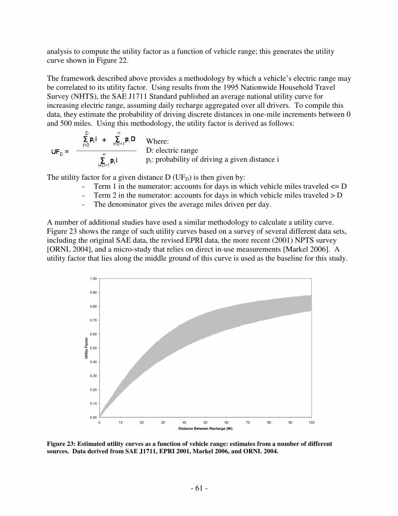
- 61 -

analysis to compute the utility factor as a function of vehicle range; this generates the utility curve shown in Figure 22. The framework described above provides a methodology by which a vehicle’s electric range may be correlated to its utility factor. Using results from the 1995 Nationwide Household Travel Survey (NHTS), the SAE J1711 Standard published an average national utility curve for increasing electric range, assuming daily recharge aggregated over all drivers. To compile this data, they estimate the probability of driving discrete distances in one-mile increments between 0 and 500 miles. Using this methodology, the utility factor is derived as follows:

Where: D: electric range pi: probability of driving a given distance i

The utility factor for a given distance D (UFD) is then given by: - Term 1 in the numerator: accounts for days in which vehicle miles traveled <= D - Term 2 in the numerator: accounts for days in which vehicle miles traveled > D - The denominator gives the average miles driven per day.

A number of additional studies have used a similar methodology to calculate a utility curve. Figure 23 shows the range of such utility curves based on a survey of several different data sets, including the original SAE data, the revised EPRI data, the more recent (2001) NPTS survey [ORNL 2004], and a micro-study that relies on direct in-use measurements [Markel 2006]. A utility factor that lies along the middle ground of this curve is used as the baseline for this study.

0.00

0.10

0.20

0.30

0.40

0.50

0.60

0.70

0.80

0.90

1.00

0 10 20 30 40 50 60 70 80 90 100

Distance Between Recharge (Mi)

Uti

lity

Fa

cto

r

Figure 23: Estimated utility curves as a function of vehicle range: estimates from a number of different sources. Data derived from SAE J1711, EPRI 2001, Markel 2006, and ORNL 2004.

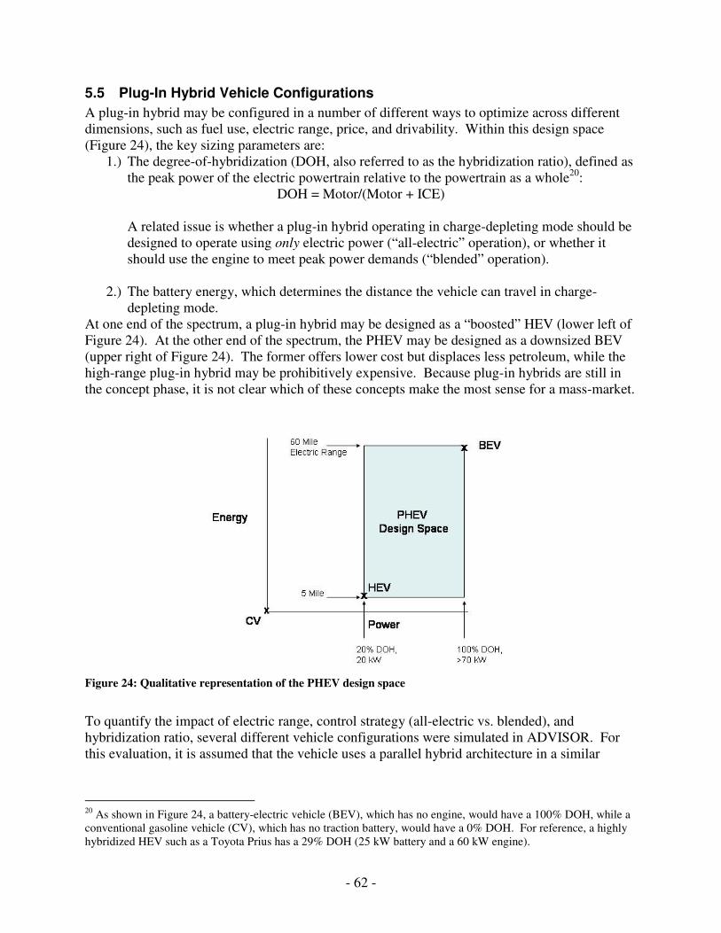
- 62 -

5.5 Plug-In Hybrid Vehicle Configurations

A plug-in hybrid may be configured in a number of different ways to optimize across different dimensions, such as fuel use, electric range, price, and drivability. Within this design space (Figure 24), the key sizing parameters are:

1.) The degree-of-hybridization (DOH, also referred to as the hybridization ratio), defined as the peak power of the electric powertrain relative to the powertrain as a whole20:

DOH = Motor/(Motor + ICE) A related issue is whether a plug-in hybrid operating in charge-depleting mode should be designed to operate using only electric power (“all-electric” operation), or whether it should use the engine to meet peak power demands (“blended” operation).

2.) The battery energy, which determines the distance the vehicle can travel in charge-

depleting mode. At one end of the spectrum, a plug-in hybrid may be designed as a “boosted” HEV (lower left of Figure 24). At the other end of the spectrum, the PHEV may be designed as a downsized BEV (upper right of Figure 24). The former offers lower cost but displaces less petroleum, while the high-range plug-in hybrid may be prohibitively expensive. Because plug-in hybrids are still in the concept phase, it is not clear which of these concepts make the most sense for a mass-market.

Figure 24: Qualitative representation of the PHEV design space

To quantify the impact of electric range, control strategy (all-electric vs. blended), and hybridization ratio, several different vehicle configurations were simulated in ADVISOR. For this evaluation, it is assumed that the vehicle uses a parallel hybrid architecture in a similar

20 As shown in Figure 24, a battery-electric vehicle (BEV), which has no engine, would have a 100% DOH, while a conventional gasoline vehicle (CV), which has no traction battery, would have a 0% DOH. For reference, a highly hybridized HEV such as a Toyota Prius has a 29% DOH (25 kW battery and a 60 kW engine).

- 63 -

configuration to that projected for the hybrid21. Such a configuration makes sense for plug-in hybrids with low- to medium electric range (i.e., “boosted HEVs”) for reasons similar to those assumed for the HEV. That said, there may be integration advantages associated with using a series architecture. While such a platform would incur additional losses in charge-sustaining mode, these losses would be minimized in vehicles with a high electric range.

5.5.1 Hybridization Ratio (All-Electric vs Blended Control Strategy)

It is still an open-question as to whether plug-in hybrids should be configured to operate in blended or all-electric mode. Because blended mode implies that the motor need not meet peak power requirements, it allows for a smaller electric powertrain. Downsizing the electric powertrain is desirable for both cost and performance reasons. On a per-kW basis, a conventional powertrain is less expensive than an electric powertrain: while energy is the primary battery cost driver, power remains a significant multiplier to the total battery cost (see Chapter 3 for more details). All-electric operation is also problematic insofar as that a vehicle would ideally offer consistent performance in both charge-depleting and charge-sustaining mode while meeting the performance constraints identified in Section 5.3 in both charge-sustaining and charge-depleting mode. In practice, these constraints limit the amount that the motor and the ICE may be downsized: This limit is fixed both by the grade-climbing requirement and by the requirement that the vehicle meet the US06 drive cycle in both driving modes. At the same time, there are compelling arguments to be made for all-electric operation. All-electric operation minimizes the number of cold-starts for the engine; this is because the engine restarts at most once per vehicle trip; in blended mode, the engine may restart a number of times to meet peak power requests. This cold-start effect may have both a fuel-consumption and pollutant emissions impact. The other important advantage of all-electric operation is that it maximizes petroleum reduction by front-loading the off-board electricity use to the initial portion of the drive cycle. For a vehicle with a large electric range, this front-loading effect can be an important consideration. To shed further light on this question of hybridization and control strategy, sensitivity analysis was performed on several different vehicle configurations. In these simulations, the vehicle’s hybridization ratio is varied from 55% (the minimum required for all-electric operation in the US06 drive cycle) down to 26% (the minimum hybrid vehicle power requirement, fixed by regenerative braking needs). The tests are based on a vehicle with a 30-mile electric range. The vehicle operating in all-electric mode is restricted from using its engine during charge depleting operation, while those operating in blended mode use electric power to the extent that it is available and covers any shortfall in transient requests using engine power. For this analysis, the powertrain power (motor + engine) is held constant at 90 kW, except for the vehicle using all-electric mode, which requires an oversized powertrain to meet performance requirements. The all-electric configuration represents a compromise between the performance requirements and the practical realities of increasing vehicle power. Minor weight differences exist between different vehicles, due in part to varying battery specific power to reflect the

21 This assumption assumes either that a closely coupled engine, motor, and transmission enables active optimization of engine operation, or that a Prius-like power-split architecture is used. See Chapter 4 or Kasseris [2006] for further details.

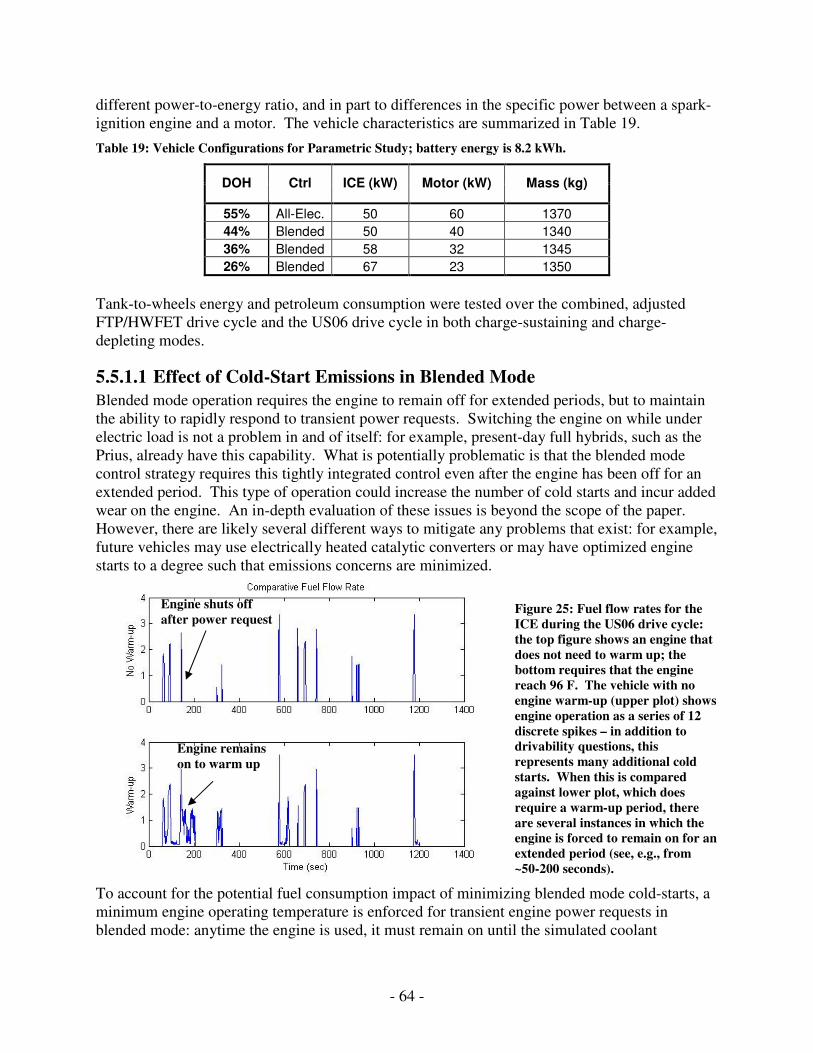
- 64 -

different power-to-energy ratio, and in part to differences in the specific power between a spark-ignition engine and a motor. The vehicle characteristics are summarized in Table 19.

Table 19: Vehicle Configurations for Parametric Study; battery energy is 8.2 kWh.

DOH Ctrl ICE (kW) Motor (kW) Mass (kg)

55% All-Elec. 50 60 1370

44% Blended 50 40 1340

36% Blended 58 32 1345

26% Blended 67 23 1350

Tank-to-wheels energy and petroleum consumption were tested over the combined, adjusted FTP/HWFET drive cycle and the US06 drive cycle in both charge-sustaining and charge-depleting modes.

5.5.1.1 Effect of Cold-Start Emissions in Blended Mode

Blended mode operation requires the engine to remain off for extended periods, but to maintain the ability to rapidly respond to transient power requests. Switching the engine on while under electric load is not a problem in and of itself: for example, present-day full hybrids, such as the Prius, already have this capability. What is potentially problematic is that the blended mode control strategy requires this tightly integrated control even after the engine has been off for an extended period. This type of operation could increase the number of cold starts and incur added wear on the engine. An in-depth evaluation of these issues is beyond the scope of the paper. However, there are likely several different ways to mitigate any problems that exist: for example, future vehicles may use electrically heated catalytic converters or may have optimized engine starts to a degree such that emissions concerns are minimized.

Figure 25: Fuel flow rates for the ICE during the US06 drive cycle: the top figure shows an engine that does not need to warm up; the bottom requires that the engine reach 96 F. The vehicle with no engine warm-up (upper plot) shows engine operation as a series of 12 discrete spikes – in addition to drivability questions, this represents many additional cold starts. When this is compared against lower plot, which does require a warm-up period, there are several instances in which the engine is forced to remain on for an extended period (see, e.g., from ~50-200 seconds).

To account for the potential fuel consumption impact of minimizing blended mode cold-starts, a minimum engine operating temperature is enforced for transient engine power requests in blended mode: anytime the engine is used, it must remain on until the simulated coolant

Engine remains on to warm up

Engine shuts off after power request

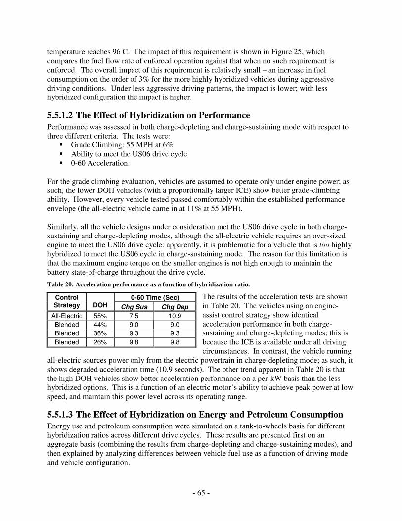
- 65 -

temperature reaches 96 C. The impact of this requirement is shown in Figure 25, which compares the fuel flow rate of enforced operation against that when no such requirement is enforced. The overall impact of this requirement is relatively small – an increase in fuel consumption on the order of 3% for the more highly hybridized vehicles during aggressive driving conditions. Under less aggressive driving patterns, the impact is lower; with less hybridized configuration the impact is higher.

5.5.1.2 The Effect of Hybridization on Performance

Performance was assessed in both charge-depleting and charge-sustaining mode with respect to three different criteria. The tests were:

Grade Climbing: 55 MPH at 6% Ability to meet the US06 drive cycle 0-60 Acceleration.

For the grade climbing evaluation, vehicles are assumed to operate only under engine power; as such, the lower DOH vehicles (with a proportionally larger ICE) show better grade-climbing ability. However, every vehicle tested passed comfortably within the established performance envelope (the all-electric vehicle came in at 11% at 55 MPH). Similarly, all the vehicle designs under consideration met the US06 drive cycle in both charge-sustaining and charge-depleting modes, although the all-electric vehicle requires an over-sized engine to meet the US06 drive cycle: apparently, it is problematic for a vehicle that is too highly hybridized to meet the US06 cycle in charge-sustaining mode. The reason for this limitation is that the maximum engine torque on the smaller engines is not high enough to maintain the battery state-of-charge throughout the drive cycle.

Table 20: Acceleration performance as a function of hybridization ratio.

The results of the acceleration tests are shown in Table 20. The vehicles using an engine-assist control strategy show identical acceleration performance in both charge-sustaining and charge-depleting modes; this is because the ICE is available under all driving circumstances. In contrast, the vehicle running

all-electric sources power only from the electric powertrain in charge-depleting mode; as such, it shows degraded acceleration time (10.9 seconds). The other trend apparent in Table 20 is that the high DOH vehicles show better acceleration performance on a per-kW basis than the less hybridized options. This is a function of an electric motor’s ability to achieve peak power at low speed, and maintain this power level across its operating range.

5.5.1.3 The Effect of Hybridization on Energy and Petroleum Consumption

Energy use and petroleum consumption were simulated on a tank-to-wheels basis for different hybridization ratios across different drive cycles. These results are presented first on an aggregate basis (combining the results from charge-depleting and charge-sustaining modes), and then explained by analyzing differences between vehicle fuel use as a function of driving mode and vehicle configuration.

0-60 Time (Sec) Control Strategy

DOH Chg Sus Chg Dep

All-Electric 55% 7.5 10.9

Blended 44% 9.0 9.0

Blended 36% 9.3 9.3

Blended 26% 9.8 9.8

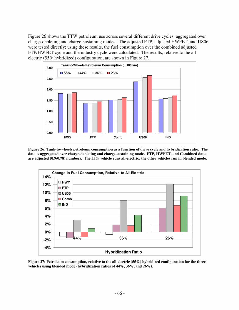
- 66 -

Figure 26 shows the TTW petroleum use across several different drive cycles, aggregated over charge-depleting and charge-sustaining modes. The adjusted FTP, adjusted HWFET, and US06 were tested directly; using these results, the fuel consumption over the combined adjusted FTP/HWFET cycle and the industry cycle were calculated. The results, relative to the all-electric (55% hybridized) configuration, are shown in Figure 27.

Tank-to-Wheels Petroleum Consumption (L/100 km)

0.00

0.50

1.00

1.50

2.00

2.50

3.00

HWY FTP Comb US06 IND

55% 44% 36% 26%

Figure 26: Tank-to-wheels petroleum consumption as a function of drive cycle and hybridization ratio. The data is aggregated over charge-depleting and charge-sustaining mode. FTP, HWFET, and Combined data are adjusted (0.9/0.78) numbers. The 55% vehicle runs all-electric; the other vehicles run in blended mode.

Change in Fuel Consumption, Relative to All-Electric

-4%

-2%

0%

2%

4%

6%

8%

10%

12%

14%

44% 36% 26%

Hybridization Ratio

HWY

FTP

US06

Comb

IND

Figure 27: Petroleum consumption, relative to the all-electric (55%) hybridized configuration for the three vehicles using blended mode (hybridization ratios of 44%, 36%, and 26%).

- 67 -

As shown in Figure 27, there is little difference between the petroleum consumption of the highly hybridized (44%) vehicle in blended mode and the all-electric baseline22. For the less hybridized vehicles, there are small differences relative to the all-electric configuration over the FTP, HWFET, and combined drive cycles. Over the US06 drive cycle, this difference is more significant. The differences between drive cycles and between vehicles configurations arise primarily due to the fact that the more highly hybridized vehicles rarely use their engine for short trips (or in the case of the all-electric vehicle, not at all). Over the FTP and HWFET drive cycles, the three more-hybridized vehicles (the 36%-blended, 44%-blended, and 55%-all-electric configurations) do not use the engine at all: the electric motor is powerful enough to meet the vehicle’s road load. As such, there is little difference between the fuel consumption. In contrast, all of the blended configurations (26%, 36%, and 44%) require engine-assist to one extent or another during the US06 cycle; in addition, the 26%-blended configuration requires engine-assist over the FTP drive cycle. The 55%-all-electric configuration, by definition, does not use the engine under any circumstances. This behavior has two relevant implications: the first is that, during charge-depleting mode, the less hybridized vehicles have much higher fuel consumption. However, because the more hybridized vehicles use stored electric power for a greater fraction of their energy in charge-depleting mode, they have a lower charge-depleting range (Table 21).

Table 21: Petroleum use, in L/100 km, in the US06 cycle, in charge-depeleting (CD) and charge-sustaining (CS) mode. The third column shows the vehicle’s range in charge-depleting mode.

The impact of these differences in engine use on petroleum consumption is shown in Figure 28. Both Figure 28 and Table 21 focus on the US06 drive cycle, in part because it emphasizes the

point, and in part because this may be a more appropriate metric for characterizing the difference between hybridization levels23. The interpretation of Figure 28 is as follows:

1.) While all vehicles are in charge-depleting mode (distances <~20 miles), fuel consumption is constant for each vehicle, but increases with decreasing hybridization ratio. This reflects the increasing reliance on the engine during charge-depleting operation.

2.) For distances between roughly 20-30 miles, the aggregate fuel consumption of the high-hybridization vehicles rises sharply (reflecting the switch from charge-depleting to charge-sustaining operation) while the less hybridized vehicles continue along the

22 The reason that the 44% vehicle performs better is due to a minor weight difference. 23 The reason that US06 is deemed more appropriate is that the standard FTP and HWFET adjustments (0.9 and 0.78), which are used to reflect “real-world” conditions, do not reflect the fact that marginal power in a blended mode plug-in hybrid come from the engine. The fixed multipliers correct for real-world driving conditions by scaling the average fuel consumption, which includes both highly efficient electric operation and peaking engine power. The aggressiveness of the US06 avoids this problem.

Configuration DOH CS CD Range

All-Electric 55% 3.90 0.00 21.8

Blended 44% 3.89 0.59 25.3

Blended 36% 3.94 0.80 25.7

Blended 26% 3.97 1.13 27.0

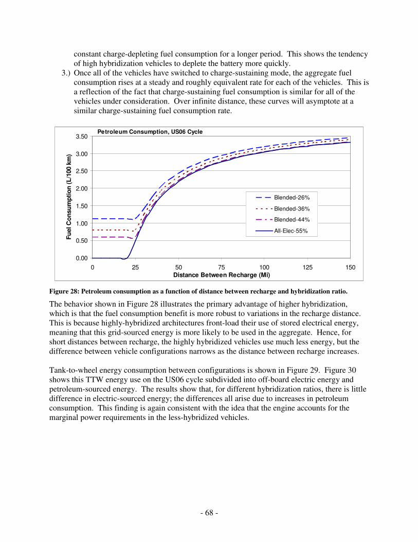
- 68 -

constant charge-depleting fuel consumption for a longer period. This shows the tendency of high hybridization vehicles to deplete the battery more quickly.

3.) Once all of the vehicles have switched to charge-sustaining mode, the aggregate fuel consumption rises at a steady and roughly equivalent rate for each of the vehicles. This is a reflection of the fact that charge-sustaining fuel consumption is similar for all of the vehicles under consideration. Over infinite distance, these curves will asymptote at a similar charge-sustaining fuel consumption rate.

Petroleum Consumption, US06 Cycle

0.00

0.50

1.00

1.50

2.00

2.50

3.00

3.50

0 25 50 75 100 125 150Distance Between Recharge (Mi)

Fu

el C

on

su

mp

tio

n (

L/1

00 k

m)

Blended-26%

Blended-36%

Blended-44%

All-Elec-55%

Figure 28: Petroleum consumption as a function of distance between recharge and hybridization ratio.

The behavior shown in Figure 28 illustrates the primary advantage of higher hybridization, which is that the fuel consumption benefit is more robust to variations in the recharge distance. This is because highly-hybridized architectures front-load their use of stored electrical energy, meaning that this grid-sourced energy is more likely to be used in the aggregate. Hence, for short distances between recharge, the highly hybridized vehicles use much less energy, but the difference between vehicle configurations narrows as the distance between recharge increases. Tank-to-wheel energy consumption between configurations is shown in Figure 29. Figure 30 shows this TTW energy use on the US06 cycle subdivided into off-board electric energy and petroleum-sourced energy. The results show that, for different hybridization ratios, there is little difference in electric-sourced energy; the differences all arise due to increases in petroleum consumption. This finding is again consistent with the idea that the engine accounts for the marginal power requirements in the less-hybridized vehicles.

- 69 -

Tank-to-Wheels Energy Use (L/100 km GE)

0.00

0.50

1.00

1.50

2.00

2.50

3.00

3.50

4.00

HWY FTP Comb US06 IND

55% 44% 36% 26%

Figure 29: Tank-to-wheels energy use as a function of drive cycle and hybridization ratio. The data is aggregated over charge-depleting and charge-sustaining mode. FTP, HWFET, and combined data are adjusted (0.9/0.78) numbers. The 55% vehicle runs all-electric; the other vehicles run in blended mode.

0.73 2.36

0.71 2.43

0.70 2.55

0.70 2.65

0.00 0.50 1.00 1.50 2.00 2.50 3.00 3.50

TTW Energy Use (L/100 km, GE)

All-Electric-55%

Blended-44%

Blended-36%

Blended-26%

Electricity Petroleum

Figure 30: Breakdown of Tank-to-Wheel (TTW) Energy Use in the US06 Cycle

5.5.1.4 Results of Hybridization Ratio Sensitivity Analysis

Table 22 summarizes the fuel consumption and performance results for the different vehicle configurations. The results of the sensitivity analysis lead to a conclusion that the vehicle’s powertrain should be sized to handle most, but not all of the road load under aggressive driving conditions. As such, the vehicle with a 44% hybridization ratio operating in blended mode is selected as a sensible configuration for subsequent tests. This conclusion is based on the

3.35

3.25

3.09

3.14

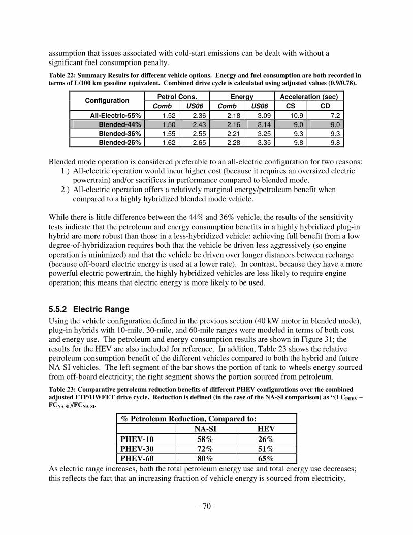
- 70 -

assumption that issues associated with cold-start emissions can be dealt with without a significant fuel consumption penalty.

Table 22: Summary Results for different vehicle options. Energy and fuel consumption are both recorded in terms of L/100 km gasoline equivalent. Combined drive cycle is calculated using adjusted values (0.9/0.78).

Petrol Cons. Energy Acceleration (sec) Configuration

Comb US06 Comb US06 CS CD

All-Electric-55% 1.52 2.36 2.18 3.09 10.9 7.2

Blended-44% 1.50 2.43 2.16 3.14 9.0 9.0

Blended-36% 1.55 2.55 2.21 3.25 9.3 9.3

Blended-26% 1.62 2.65 2.28 3.35 9.8 9.8

Blended mode operation is considered preferable to an all-electric configuration for two reasons:

1.) All-electric operation would incur higher cost (because it requires an oversized electric powertrain) and/or sacrifices in performance compared to blended mode.

2.) All-electric operation offers a relatively marginal energy/petroleum benefit when compared to a highly hybridized blended mode vehicle.

While there is little difference between the 44% and 36% vehicle, the results of the sensitivity tests indicate that the petroleum and energy consumption benefits in a highly hybridized plug-in hybrid are more robust than those in a less-hybridized vehicle: achieving full benefit from a low degree-of-hybridization requires both that the vehicle be driven less aggressively (so engine operation is minimized) and that the vehicle be driven over longer distances between recharge (because off-board electric energy is used at a lower rate). In contrast, because they have a more powerful electric powertrain, the highly hybridized vehicles are less likely to require engine operation; this means that electric energy is more likely to be used.

5.5.2 Electric Range

Using the vehicle configuration defined in the previous section (40 kW motor in blended mode), plug-in hybrids with 10-mile, 30-mile, and 60-mile ranges were modeled in terms of both cost and energy use. The petroleum and energy consumption results are shown in Figure 31; the results for the HEV are also included for reference. In addition, Table 23 shows the relative petroleum consumption benefit of the different vehicles compared to both the hybrid and future NA-SI vehicles. The left segment of the bar shows the portion of tank-to-wheels energy sourced from off-board electricity; the right segment shows the portion sourced from petroleum.

Table 23: Comparative petroleum reduction benefits of different PHEV configurations over the combined adjusted FTP/HWFET drive cycle. Reduction is defined (in the case of the NA-SI comparison) as “(FCPHEV – FCNA-SI)/FCNA-SI.

% Petroleum Reduction, Compared to:

NA-SI HEV

PHEV-10 58% 26% PHEV-30 72% 51% PHEV-60 80% 65%

As electric range increases, both the total petroleum energy use and total energy use decreases; this reflects the fact that an increasing fraction of vehicle energy is sourced from electricity,

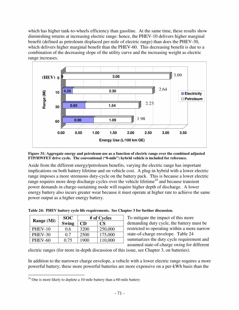
- 71 -

which has higher tank-to-wheels efficiency than gasoline. At the same time, these results show diminishing returns at increasing electric range: hence, the PHEV-10 delivers higher marginal benefit (defined as petroleum displaced per-mile of electric range) than does the PHEV-30, which delivers higher marginal benefit than the PHEV-60. This decreasing benefit is due to a combination of the decreasing slope of the utility curve and the increasing weight as electric range increases.

0.90 1.09

0.65 1.54

0.29 2.30

0 3.08

0.00 0.50 1.00 1.50 2.00 2.50 3.00 3.50

Energy Use (L/100 km GE)

60

30

10

0

Ra

ng

e (

Mi)

Electricity

Petroleum

Figure 31: Aggregate energy and petroleum use as a function of electric range over the combined adjusted FTP/HWFET drive cycle. The conventional (“0-mile”) hybrid vehicle is included for reference.

Aside from the different energy/petroleum benefits, varying the electric range has important implications on both battery lifetime and on vehicle cost. A plug-in hybrid with a lower electric range imposes a more strenuous duty-cycle on the battery pack. This is because a lower electric range requires more deep discharge cycles over the vehicle lifetime24 and because transient power demands in charge-sustaining mode will require higher depth of discharge. A lower energy battery also incurs greater wear because it must operate at higher rate to achieve the same power output as a higher energy battery.

Table 24: PHEV battery cycle life requirements. See Chapter 3 for further discussion.

To mitigate the impact of this more demanding duty cycle, the battery must be restricted to operating within a more narrow state-of-charge envelope. Table 24 summarizes the duty cycle requirement and assumed state-of-charge swing for different

electric ranges (for more in-depth discussion of this issue, see Chapter 3, on batteries). In addition to the narrower charge envelope, a vehicle with a lower electric range requires a more powerful battery; these more powerful batteries are more expensive on a per-kWh basis than the

24 One is more likely to deplete a 10-mile battery than a 60-mile battery

# of Cycles Range (Mi)

SOC Swing CD CS

PHEV-10 0.6 3200 250,000

PHEV-30 0.7 2500 175,000

PHEV-60 0.75 1900 110,000

3.09

2.64

2.23

1.98

(HEV)

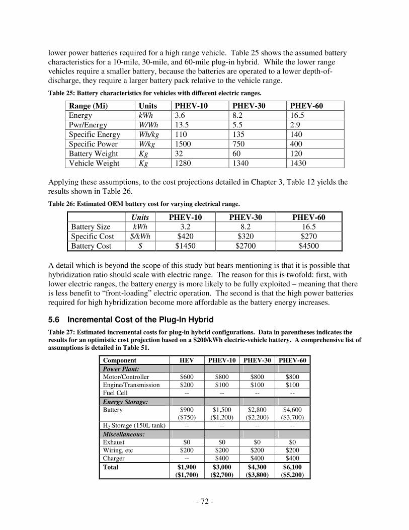
- 72 -

lower power batteries required for a high range vehicle. Table 25 shows the assumed battery characteristics for a 10-mile, 30-mile, and 60-mile plug-in hybrid. While the lower range vehicles require a smaller battery, because the batteries are operated to a lower depth-of-discharge, they require a larger battery pack relative to the vehicle range.

Table 25: Battery characteristics for vehicles with different electric ranges.

Range (Mi) Units PHEV-10 PHEV-30 PHEV-60 Energy kWh 3.6 8.2 16.5

Pwr/Energy W/Wh 13.5 5.5 2.9

Specific Energy Wh/kg 110 135 140

Specific Power W/kg 1500 750 400

Battery Weight Kg 32 60 120

Vehicle Weight Kg 1280 1340 1430

Applying these assumptions, to the cost projections detailed in Chapter 3, Table 12 yields the results shown in Table 26.

Table 26: Estimated OEM battery cost for varying electrical range.

Units PHEV-10 PHEV-30 PHEV-60 Battery Size kWh 3.2 8.2 16.5

Specific Cost $/kWh $420 $320 $270

Battery Cost $ $1450 $2700 $4500

A detail which is beyond the scope of this study but bears mentioning is that it is possible that hybridization ratio should scale with electric range. The reason for this is twofold: first, with lower electric ranges, the battery energy is more likely to be fully exploited – meaning that there is less benefit to “front-loading” electric operation. The second is that the high power batteries required for high hybridization become more affordable as the battery energy increases.

5.6 Incremental Cost of the Plug-In Hybrid

Table 27: Estimated incremental costs for plug-in hybrid configurations. Data in parentheses indicates the results for an optimistic cost projection based on a $200/kWh electric-vehicle battery. A comprehensive list of assumptions is detailed in Table 51.

Component HEV PHEV-10 PHEV-30 PHEV-60

Power Plant:

Motor/Controller $600 $800 $800 $800

Engine/Transmission $200 $100 $100 $100

Fuel Cell -- -- -- --

Energy Storage:

Battery $900 ($750)

$1,500 ($1,200)

$2,800 ($2,200)

$4,600 ($3,700)

H2 Storage (150L tank) -- -- -- --

Miscellaneous:

Exhaust $0 $0 $0 $0

Wiring, etc $200 $200 $200 $200

Charger -- $400 $400 $400

Total $1,900 ($1,700)

$3,000 ($2,700)

$4,300 ($3,800)

$6,100 ($5,200)

- 73 -

The incremental costs of the plug-in hybrid are based on a similar logic and similar assumptions to those used for the conventional hybrid. A component-by-component breakdown for the different vehicle configurations is shown in Table 27. Battery costs are based on the data shown in Table 26. Differences between the plug-in hybrid and hybrid costs arise primarily from the larger battery; in addition, the plug-in hybrids require an onboard charger, but receive an extra $100 credit for further downsizing the engine.

5.6.1 Cost-Effectiveness of Varying Electric Range

One way to quantify the cost-effectiveness of the different vehicle configurations is to calculate the cost per liter of gasoline saved, as compared to the hybrid and conventional vehicle. Applying this metric gives results as shown in Table 28; both the base case and optimistic battery cost projections are shown.

Table 28: Comparative cost-effectiveness of different PHEV configurations, as compared to the HEV and NA-SI. Results are based on a vehicle lifetime of 150,000 miles. Parentheses indicate the incremental cost for the optimistic cost projection. A comprehensive list of assumptions is detailed in Table 51.

$/L Saved, Compared to NA-SI

$/L Saved, Compared to HEV

Incremental

Cost Fuel Used

(L) Base Case Optimistic Base Case Optimistic

NA-SI - 13,200 -- -- -- --

HEV $1,900 ($1,700)

7,500 $0.33 $0.30 -- --

PHEV-10 $3,000 ($2,700)

5,800 $0.39 $0.35 $0.57 $0.52

PHEV-30 $4,300 ($3,800)

3,900 $0.45 $0.40 $0.64 $0.56

PHEV-60 $6,100 ($5,200)

2,600 $0.58 $0.49 $0.87 $0.73

This calculation suggests that the marginal cost-effectiveness of the hybrid vehicle is significantly greater than any of the plug-in hybrid configurations. This is apparent when the $/L saved compared to the NA-SI is compared to that of the $/L saved compared to the hybrid: the former range from $0.39-$.58 per liter, while the latter range from $0.56 to $0.73 per liter. In a purely economic sense, it is not clear that the marginal benefit of going from the HEV to the plug-in hybrid is justified. There is no clear winner when comparing between the different PHEV configurations. The HEV-10 has the lowest marginal cost and is the most cost-effective, although not by a huge amount. In addition, this analysis does not account for the increased battery wear incurred from a smaller battery pack; nor does it account for the greater overall benefit. In light of these results, the PHEV-30 is chosen going forward as a viable middle ground for the vehicle’s electric range. This is not meant to suggest that other range configurations do not make sense (in all likelihood, there would be several different options available), but rather that a 30-mile range represents a reasonable tradeoff between cost and utility.

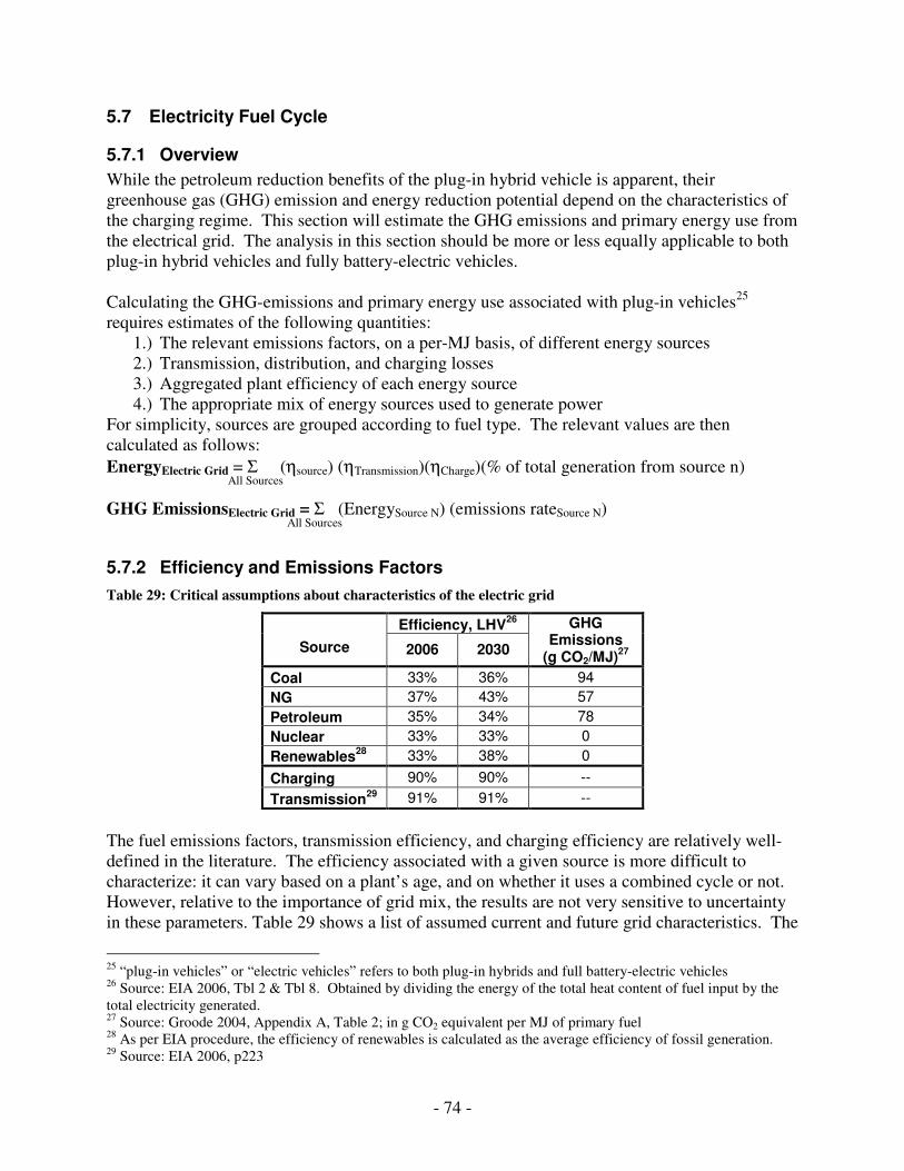
- 74 -

5.7 Electricity Fuel Cycle

5.7.1 Overview

While the petroleum reduction benefits of the plug-in hybrid vehicle is apparent, their greenhouse gas (GHG) emission and energy reduction potential depend on the characteristics of the charging regime. This section will estimate the GHG emissions and primary energy use from the electrical grid. The analysis in this section should be more or less equally applicable to both plug-in hybrid vehicles and fully battery-electric vehicles. Calculating the GHG-emissions and primary energy use associated with plug-in vehicles25 requires estimates of the following quantities:

1.) The relevant emissions factors, on a per-MJ basis, of different energy sources 2.) Transmission, distribution, and charging losses 3.) Aggregated plant efficiency of each energy source 4.) The appropriate mix of energy sources used to generate power

For simplicity, sources are grouped according to fuel type. The relevant values are then calculated as follows:

EnergyElectric Grid = Σ (ηsource) (ηTransmission)(ηCharge)(% of total generation from source n) All Sources

GHG EmissionsElectric Grid = Σ (EnergySource N) (emissions rateSource N) All Sources

5.7.2 Efficiency and Emissions Factors

Table 29: Critical assumptions about characteristics of the electric grid

Efficiency, LHV26

Source 2006 2030

GHG Emissions

(g CO2/MJ)27

Coal 33% 36% 94

NG 37% 43% 57

Petroleum 35% 34% 78

Nuclear 33% 33% 0

Renewables28

33% 38% 0

Charging 90% 90% --

Transmission29

91% 91% --

The fuel emissions factors, transmission efficiency, and charging efficiency are relatively well-defined in the literature. The efficiency associated with a given source is more difficult to characterize: it can vary based on a plant’s age, and on whether it uses a combined cycle or not. However, relative to the importance of grid mix, the results are not very sensitive to uncertainty in these parameters. Table 29 shows a list of assumed current and future grid characteristics. The

25 “plug-in vehicles” or “electric vehicles” refers to both plug-in hybrids and full battery-electric vehicles 26 Source: EIA 2006, Tbl 2 & Tbl 8. Obtained by dividing the energy of the total heat content of fuel input by the total electricity generated. 27 Source: Groode 2004, Appendix A, Table 2; in g CO2 equivalent per MJ of primary fuel 28 As per EIA procedure, the efficiency of renewables is calculated as the average efficiency of fossil generation. 29 Source: EIA 2006, p223

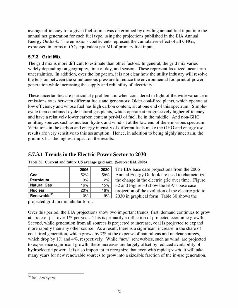
- 75 -

average efficiency for a given fuel source was determined by dividing annual fuel input into the annual net generation for each fuel type, using the projections published in the EIA Annual Energy Outlook. The emissions coefficients represent the cumulative effect of all GHGs, expressed in terms of CO2-equivalent per MJ of primary fuel input.

5.7.3 Grid Mix

The grid mix is more difficult to estimate than other factors. In general, the grid mix varies widely depending on geography, time of day, and season. These represent localized, near-term uncertainties. In addition, over the long-term, it is not clear how the utility industry will resolve the tension between the simultaneous pressure to reduce the environmental footprint of power generation while increasing the supply and reliability of electricity. These uncertainties are particularly problematic when considered in light of the wide variance in emissions rates between different fuels and generators: Older coal-fired plants, which operate at low efficiency and whose fuel has high carbon content, sit at one end of this spectrum. Simple-cycle then combined-cycle natural gas plants, which operate at progressively higher efficiency and have a relatively lower carbon content per-MJ of fuel, lie in the middle. And non-GHG emitting sources such as nuclear, hydro, and wind sit at the low end of the emissions spectrum. Variations in the carbon and energy intensity of different fuels make the GHG and energy use results are very sensitive to this assumption. Hence, in addition to being highly uncertain, the grid mix has the highest impact on the results.

5.7.3.1 Trends in the Electric Power Sector to 2030

Table 30: Current and future US average grid mix. (Source: EIA 2006)

The EIA base case projections from the 2006 Annual Energy Outlook are used to characterize the change in the electric grid over time. Figure 32 and Figure 33 show the EIA’s base case projection of the evolution of the electric grid to 2030 in graphical form; Table 30 shows the

projected grid mix in tabular form. Over this period, the EIA projections show two important trends: first, demand continues to grow at a rate of just over 1% per year. This is primarily a reflection of projected economic growth. Second, while generation from all sources is projected to increase, coal is projected to expand more rapidly than any other source. As a result, there is a significant increase in the share of coal-fired generation, which grows by 7% at the expense of natural gas and nuclear sources, which drop by 1% and 4%, respectively. While “new” renewables, such as wind, are projected to experience significant growth, these increases are largely offset by reduced availability of hydroelectric power. It is also important to recognize that even with rapid growth, it will take many years for new renewable sources to grow into a sizeable fraction of the in-use generation.

30 Includes hydro

2006 2030

Coal 52% 58%

Petroleum 3% 2%

Natural Gas 16% 15%

Nuclear 20% 16%

Renewable30

10% 9%

- 76 -

% of Net Generation

Coal

Nuclear

Gas

Renewables

Oil

0%

10%

20%

30%

40%

50%

60%

70%

80%

90%

100%

2005 2010 2015 2020 2025 2030

Figure 32: Evolution of US Average Grid Mix, 2005-2030. Source: EIA 2006

Net Generation (B kWh)

Coal

Nuclear

Gas

Renewables

Oil

0

1000

2000

3000

4000

5000

6000

2005 2010 2015 2020 2025 2030

Figure 33: Projected US electricity generation by source, 2005-2030. Source: EIA 2006

The net result of these trends – in particular, the changing grid mix shown in Table 30 and the improved efficiency shown in Table 29 – is that the emissions rate of the electric grid does not change substantially over the next several decades according to the EIA estimates. This is because the increasing efficiency of the grid over time (as old units are replaced with newer ones) is offset by the increasing share of coal within the overall grid mix. The base case

- 77 -

assumptions give an average grid emissions rate of 635g CO2/MWh generated for the 2030 grid, as compared to 640g CO2/MWh in the present31. While the business-as-usual projection does not project substantive improvements to the emissions rate of the electric grid, there is a strong likelihood that other factors will come into play over the next several decades. Several such factors are summarized in Table 31; the impact of these trends could act to decrease or increase this emissions rate. In addition, there are potential synergies between plug-in loads and intermittent renewables which could enable greater market penetration of these resources.

Table 31: Trends in the utility sector and their impact on the base-case projections

Key Electric Sector Drivers Qualitative Impact Monetization of CO2 Increases low-carbon generation

Renewable Portfolio Stds (RPS) Increases low-carbon baseload generation

Demand-side reduction May increase or decrease emissions rate, depending on whether coal or low-emitting sources are the first choice to meet demand growth

Utility restructuring Uncertain impact: could lower barriers to entry for new sources or drive market towards lowest cost source (typically coal)

Price volatility of natural gas Drives market away from natural gas towards coal

Difficulty siting nuclear, coal, and wind Varies

While the EIA base case projections are used to calculate baseline estimates of the grid emissions, due to the uncertainty introduced by these pressures, a range of GHG emissions estimates is provided to show the impact of using different assumptions.

5.7.3.2 Grid Dispatch

Characterizing the emissions impact of charging an electric vehicle from the grid requires a more subtle assessment than simply projecting the average grid mix into the future. To illustrate this point, it is important to understand the mechanics of electric grid dispatch. The demand for generation varies widely depending on time of day and season. To meet this varying demand, a variety of generators with different load-following capabilities are needed. These generators are generally dispatched in economic merit order (from lowest variable cost to highest). The low-cost baseload generators are comprised of nuclear, hydro-electric, and some coal plants. In addition, non-dispatchable resources such as intermittent renewables are used whenever they are available. After these baseload resources, higher variable cost units such as natural gas (especially combined-cycle natural gas) and older coal plants are used to respond to intermediate power requests. The highest cost but most responsive resources are typically combustion turbines running on gas or oil; these are used to respond to short-term peaks in demand [Kintner-Meyer 2006].

31 These values do not account for transmission, distribution, or charging losses.

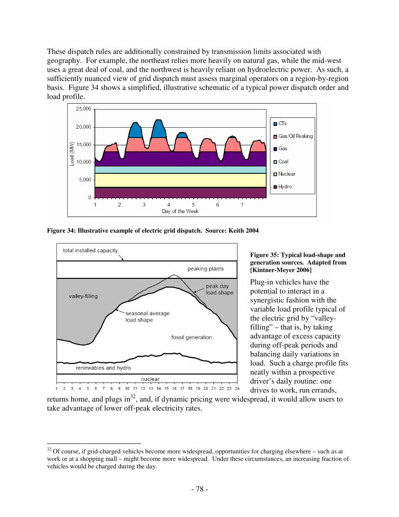
- 78 -

These dispatch rules are additionally constrained by transmission limits associated with geography. For example, the northeast relies more heavily on natural gas, while the mid-west uses a great deal of coal, and the northwest is heavily reliant on hydroelectric power. As such, a sufficiently nuanced view of grid dispatch must assess marginal operators on a region-by-region basis. Figure 34 shows a simplified, illustrative schematic of a typical power dispatch order and load profile.

Figure 34: Illustrative example of electric grid dispatch. Source: Keith 2004

Figure 35: Typical load-shape and generation sources. Adapted from [Kintner-Meyer 2006]

Plug-in vehicles have the potential to interact in a synergistic fashion with the variable load profile typical of the electric grid by “valley-filling” – that is, by taking advantage of excess capacity during off-peak periods and balancing daily variations in load. Such a charge profile fits neatly within a prospective driver’s daily routine: one drives to work, run errands,

returns home, and plugs in32, and, if dynamic pricing were widespread, it would allow users to take advantage of lower off-peak electricity rates.

32 Of course, if grid-charged vehicles become more widespread, opportunities for charging elsewhere – such as at work or at a shopping mall – might become more widespread. Under these circumstances, an increasing fraction of vehicles would be charged during the day.

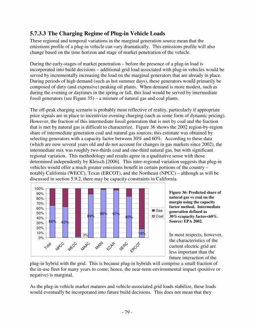
- 79 -

66% 63%

89%98% 97%

85%

18%3%

0%

10%

20%

30%

40%

50%

60%

70%

80%

90%

100%

Total

NPC

C

WECC

MAAC

MAIN

ECAR

SERC

ERCOT

Gas

Coal

5.7.3.3 The Charging Regime of Plug-in Vehicle Loads

These regional and temporal variations in the marginal generation source mean that the emissions profile of a plug-in vehicle can vary dramatically. This emissions profile will also change based on the time horizon and stage of market penetration of the vehicle. During the early-stages of market penetration – before the presence of a plug-in load is incorporated into build decisions – additional grid load associated with plug-in vehicles would be served by incrementally increasing the load on the marginal generators that are already in place. During periods of high demand (such as hot summer days), these generators would primarily be composed of dirty (and expensive) peaking oil plants. When demand is more modest, such as during the evening or daytimes in the spring or fall, this load would be served by intermediate fossil generators (see Figure 35) – a mixture of natural gas and coal plants. The off-peak charging scenario is probably most reflective of reality, particularly if appropriate price signals are in place to incentivize evening charging (such as some form of dynamic pricing). However, the fraction of this intermediate fossil generation that is met by coal and the fraction that is met by natural gas is difficult to characterize. Figure 36 shows the 2002 region-by-region share of intermediate generation coal and natural gas sources; this estimate was obtained by selecting generators with a capacity factor between 30% and 60%. According to these data (which are now several years old and do not account for changes in gas markets since 2002), the intermediate mix was roughly two-thirds coal and one-third natural gas, but with significant regional variation. This methodology and results agree in a qualitative sense with those determined independently by Kleisch [2006]. This inter-regional variation suggests that plug-in vehicles would offer a much greater emissions benefit in certain portions of the country – notably California (WECC), Texas (ERCOT), and the Northeast (NPCC) – although as will be discussed in section 5.9.2, there may be capacity constraints in California.

Figure 36: Predicted share of natural gas vs coal on the margin using the capacity factor method. Intermediate generation defined as 30%<capacity factor<60%. Source: EPA 2002.

In most respects, however, the characteristics of the current electric grid are less important than the future interaction of the

plug-in hybrid with the grid. This is because plug-in hybrids will comprise a small fraction of the in-use fleet for many years to come; hence, the near-term environmental impact (positive or negative) is marginal. As the plug-in vehicle market matures and vehicle-associated grid loads stabilize, these loads would eventually be incorporated into future build decisions. This does not mean that they

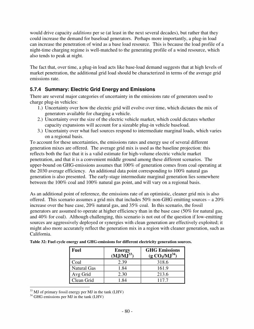
- 80 -

would drive capacity additions per se (at least in the next several decades), but rather that they could increase the demand for baseload generators. Perhaps more importantly, a plug-in load can increase the penetration of wind as a base load resource. This is because the load profile of a night-time charging regime is well-matched to the generating profile of a wind resource, which also tends to peak at night. The fact that, over time, a plug-in load acts like base-load demand suggests that at high levels of market penetration, the additional grid load should be characterized in terms of the average grid emissions rate.

5.7.4 Summary: Electric Grid Energy and Emissions

There are several major categories of uncertainty in the emissions rate of generators used to charge plug-in vehicles:

1.) Uncertainty over how the electric grid will evolve over time, which dictates the mix of generators available for charging a vehicle.

2.) Uncertainty over the size of the electric vehicle market, which could dictates whether capacity expansions will account for a sizeable plug-in vehicle baseload.

3.) Uncertainty over what fuel sources respond to intermediate marginal loads, which varies on a regional basis.

To account for these uncertainties, the emissions rates and energy use of several different generation mixes are offered. The average grid mix is used as the baseline projection: this reflects both the fact that it is a valid estimate for high-volume electric vehicle market penetration, and that it is a convenient middle ground among these different scenarios. The upper-bound on GHG-emissions assumes that 100% of generation comes from coal operating at the 2030 average efficiency. An additional data point corresponding to 100% natural gas generation is also presented. The early-stage intermediate marginal generation lies somewhere between the 100% coal and 100% natural gas point, and will vary on a regional basis. As an additional point of reference, the emissions rate of an optimistic, cleaner grid mix is also offered. This scenario assumes a grid mix that includes 50% non-GHG emitting sources – a 20% increase over the base case, 20% natural gas, and 35% coal. In this scenario, the fossil generators are assumed to operate at higher efficiency than in the base case (50% for natural gas, and 40% for coal). Although challenging, this scenario is not out of the question if low-emitting sources are aggressively deployed or synergies with clean generation are effectively exploited; it might also more accurately reflect the generation mix in a region with cleaner generation, such as California.

Table 32: Fuel cycle energy and GHG-emissions for different electricity generation sources.

Fuel Energy (MJ/MJ33)

GHG Emissions (g CO2/MJ34)

Coal 2.39 318.6

Natural Gas 1.84 161.9

Avg Grid 2.30 213.6

Clean Grid 1.84 117.7

33 MJ of primary fossil energy per MJ in the tank (LHV) 34 GHG emissions per MJ in the tank (LHV)

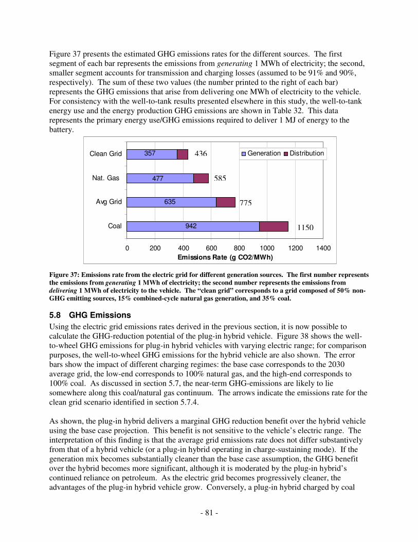
- 81 -

Figure 37 presents the estimated GHG emissions rates for the different sources. The first segment of each bar represents the emissions from generating 1 MWh of electricity; the second, smaller segment accounts for transmission and charging losses (assumed to be 91% and 90%, respectively). The sum of these two values (the number printed to the right of each bar) represents the GHG emissions that arise from delivering one MWh of electricity to the vehicle. For consistency with the well-to-tank results presented elsewhere in this study, the well-to-tank energy use and the energy production GHG emissions are shown in Table 32. This data represents the primary energy use/GHG emissions required to deliver 1 MJ of energy to the battery.

357

477

635

942

0 200 400 600 800 1000 1200 1400

Coal

Avg Grid

Nat. Gas

Clean Grid

Emissions Rate (g CO2/MWh)

Generation Distribution

Figure 37: Emissions rate from the electric grid for different generation sources. The first number represents the emissions from generating 1 MWh of electricity; the second number represents the emissions from delivering 1 MWh of electricity to the vehicle. The “clean grid” corresponds to a grid composed of 50% non-GHG emitting sources, 15% combined-cycle natural gas generation, and 35% coal.

5.8 GHG Emissions

Using the electric grid emissions rates derived in the previous section, it is now possible to calculate the GHG-reduction potential of the plug-in hybrid vehicle. Figure 38 shows the well-to-wheel GHG emissions for plug-in hybrid vehicles with varying electric range; for comparison purposes, the well-to-wheel GHG emissions for the hybrid vehicle are also shown. The error bars show the impact of different charging regimes: the base case corresponds to the 2030 average grid, the low-end corresponds to 100% natural gas, and the high-end corresponds to 100% coal. As discussed in section 5.7, the near-term GHG-emissions are likely to lie somewhere along this coal/natural gas continuum. The arrows indicate the emissions rate for the clean grid scenario identified in section 5.7.4. As shown, the plug-in hybrid delivers a marginal GHG reduction benefit over the hybrid vehicle using the base case projection. This benefit is not sensitive to the vehicle’s electric range. The interpretation of this finding is that the average grid emissions rate does not differ substantively from that of a hybrid vehicle (or a plug-in hybrid operating in charge-sustaining mode). If the generation mix becomes substantially cleaner than the base case assumption, the GHG benefit over the hybrid becomes more significant, although it is moderated by the plug-in hybrid’s continued reliance on petroleum. As the electric grid becomes progressively cleaner, the advantages of the plug-in hybrid vehicle grow. Conversely, a plug-in hybrid charged by coal

1150

775

585

436

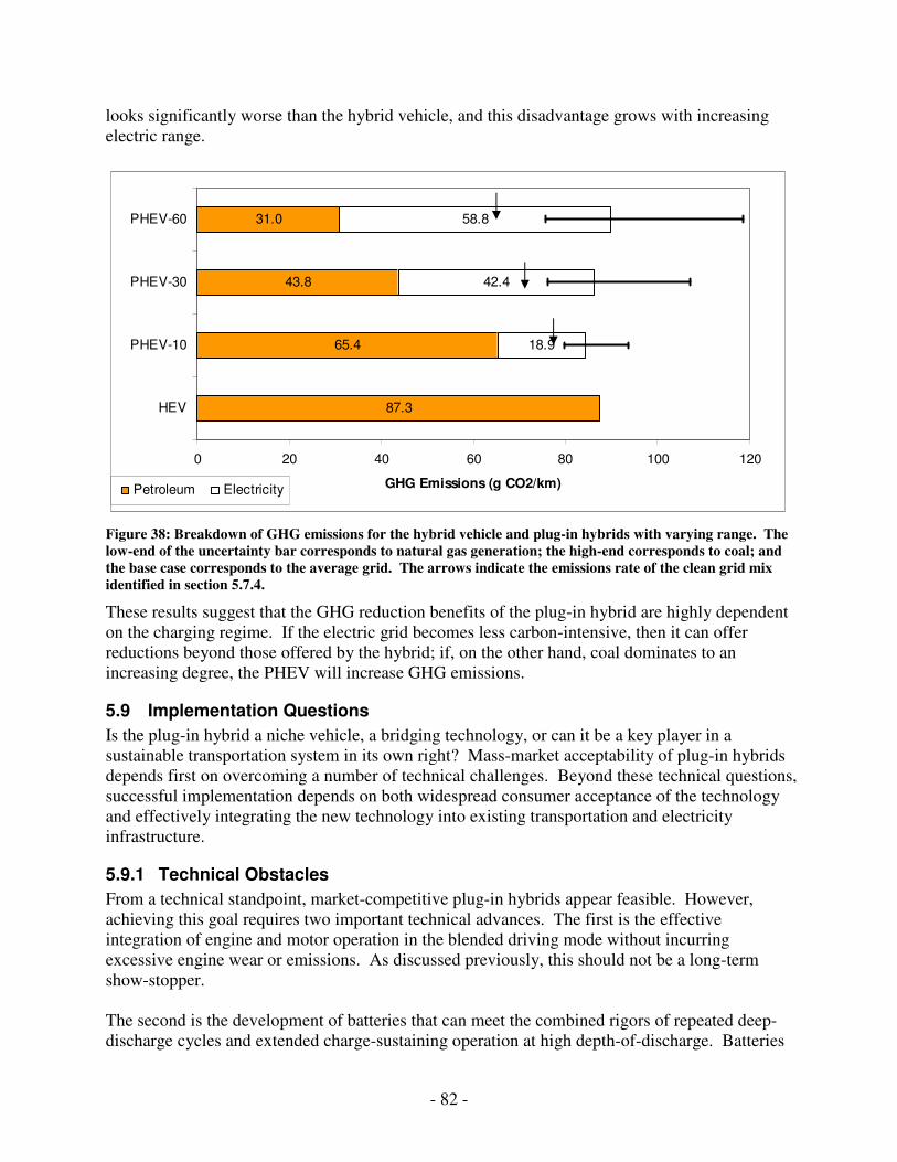
- 82 -

looks significantly worse than the hybrid vehicle, and this disadvantage grows with increasing electric range.

87.3

65.4

43.8

31.0

18.9

42.4

58.8

0 20 40 60 80 100 120

HEV

PHEV-10

PHEV-30

PHEV-60

GHG Emissions (g CO2/km)Petroleum Electricity

Figure 38: Breakdown of GHG emissions for the hybrid vehicle and plug-in hybrids with varying range. The low-end of the uncertainty bar corresponds to natural gas generation; the high-end corresponds to coal; and the base case corresponds to the average grid. The arrows indicate the emissions rate of the clean grid mix identified in section 5.7.4.

These results suggest that the GHG reduction benefits of the plug-in hybrid are highly dependent on the charging regime. If the electric grid becomes less carbon-intensive, then it can offer reductions beyond those offered by the hybrid; if, on the other hand, coal dominates to an increasing degree, the PHEV will increase GHG emissions.

5.9 Implementation Questions

Is the plug-in hybrid a niche vehicle, a bridging technology, or can it be a key player in a sustainable transportation system in its own right? Mass-market acceptability of plug-in hybrids depends first on overcoming a number of technical challenges. Beyond these technical questions, successful implementation depends on both widespread consumer acceptance of the technology and effectively integrating the new technology into existing transportation and electricity infrastructure.

5.9.1 Technical Obstacles

From a technical standpoint, market-competitive plug-in hybrids appear feasible. However, achieving this goal requires two important technical advances. The first is the effective integration of engine and motor operation in the blended driving mode without incurring excessive engine wear or emissions. As discussed previously, this should not be a long-term show-stopper. The second is the development of batteries that can meet the combined rigors of repeated deep-discharge cycles and extended charge-sustaining operation at high depth-of-discharge. Batteries

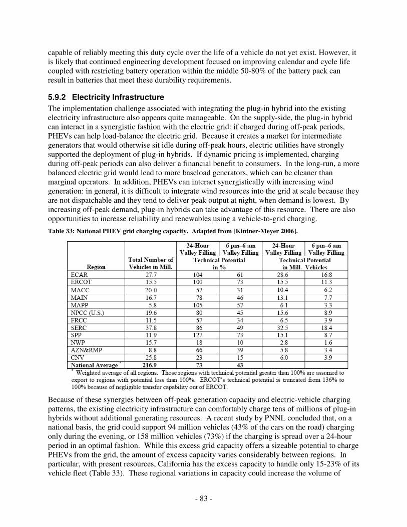
- 83 -

capable of reliably meeting this duty cycle over the life of a vehicle do not yet exist. However, it is likely that continued engineering development focused on improving calendar and cycle life coupled with restricting battery operation within the middle 50-80% of the battery pack can result in batteries that meet these durability requirements.

5.9.2 Electricity Infrastructure

The implementation challenge associated with integrating the plug-in hybrid into the existing electricity infrastructure also appears quite manageable. On the supply-side, the plug-in hybrid can interact in a synergistic fashion with the electric grid: if charged during off-peak periods, PHEVs can help load-balance the electric grid. Because it creates a market for intermediate generators that would otherwise sit idle during off-peak hours, electric utilities have strongly supported the deployment of plug-in hybrids. If dynamic pricing is implemented, charging during off-peak periods can also deliver a financial benefit to consumers. In the long-run, a more balanced electric grid would lead to more baseload generators, which can be cleaner than marginal operators. In addition, PHEVs can interact synergistically with increasing wind generation: in general, it is difficult to integrate wind resources into the grid at scale because they are not dispatchable and they tend to deliver peak output at night, when demand is lowest. By increasing off-peak demand, plug-in hybrids can take advantage of this resource. There are also opportunities to increase reliability and renewables using a vehicle-to-grid charging.

Table 33: National PHEV grid charging capacity. Adapted from [Kintner-Meyer 2006].

Because of these synergies between off-peak generation capacity and electric-vehicle charging patterns, the existing electricity infrastructure can comfortably charge tens of millions of plug-in hybrids without additional generating resources. A recent study by PNNL concluded that, on a national basis, the grid could support 94 million vehicles (43% of the cars on the road) charging only during the evening, or 158 million vehicles (73%) if the charging is spread over a 24-hour period in an optimal fashion. While this excess grid capacity offers a sizeable potential to charge PHEVs from the grid, the amount of excess capacity varies considerably between regions. In particular, with present resources, California has the excess capacity to handle only 15-23% of its vehicle fleet (Table 33). These regional variations in capacity could increase the volume of

- 84 -

electricity imported between regions (and could make California’s clean grid look much worse!) [Kintner-Meyer 2006]. Even so, the over-arching point is that, if appropriately managed, these constraints will not be a burden for decades to come. On the end-user side, the plug-in hybrid can be widely implemented without substantive upgrades to existing infrastructure. The energy of the PHEV battery is such that it can be recharged using standard household sockets overnight. For example, the 30-mile PHEV charging on a standard 120 V, 15A outlet charging at 90% efficiency can fully recharge in less than 4 hours35. According to a recent household survey, 75% of the population parks their vehicle in either a driveway, a garage, or a carport; it is not clear what fraction of these households already have an existing outlet, but upgrades could be made at relatively low cost [Wall 2006]. Some consumers may desire more rapid recharge than that offered by a standard outlet; a 220V, 30A outlet would charge in about 1.5 hours, and cost a couple of hundred dollars to upgrade [Duvall 2003]. From an infrastructure point-of-view, the primary question is how to ensure that consumers take advantage of off-peak charging. This can likely be handled with a combination of time-of-use pricing (which sends a price signal that off-peak charging is desirable), consumer education, and intelligent battery chargers. A transition to time-of-use pricing would entail upgrading consumer electric meters. Such a policy decision has implications that go well beyond the deployment of plug-in vehicles, but has been proposed as a tool to reduce peak-load demand which is justified in its own right. Many utilities already offer time-of-use pricing as an option for residential customers. On balance, these infrastructure issues pale in comparison to those faced by either hydrogen fuel-cell or fully electric vehicles. The fuel-cell would require a mature hydrogen distribution and fueling network to reach a mass-market. And while the electric vehicle can function to some extent within the current infrastructure, its high energy battery and limited range would likely require widespread availability of fast-recharge stations and capacity additions to the grid for mass-market deployment.

5.9.3 Consumer Response and Costs of Ownership

Beyond the challenges associated with technological development and managing the electricity infrastructure – which are largely issues for the auto industry and utility industry, respectively – the success of plug-in hybrids depends on consumer response to a new technology, both in terms of willingness to pay and how the technology gets used. As a prerequisite for widespread adoption, manufacturers will likely have to warranty the plug-in hybrid battery pack for the life of the vehicle. Even with this assurance that the technology meets automotive requirements, it is unlikely that, as a group, consumers will be willing to pay the steep price increment to go from the HEV to the plug-in hybrid without additional incentives. Even with significant decreases in battery costs from today’s levels, PHEVs are likely to cost $1000-$3000 more than a hybrid vehicle, and $3000-$5000 more than a conventional vehicle 5.6). It is unlikely that high gas prices alone can drive this willingness to pay (see Table 34 for a sample calculation). Consumers typically expect rapid payback on energy efficiency

35 (8.2 kWh) x (80% max depth-of-discharge) / (120 V x 15A x 0.9) = 3.3 hours

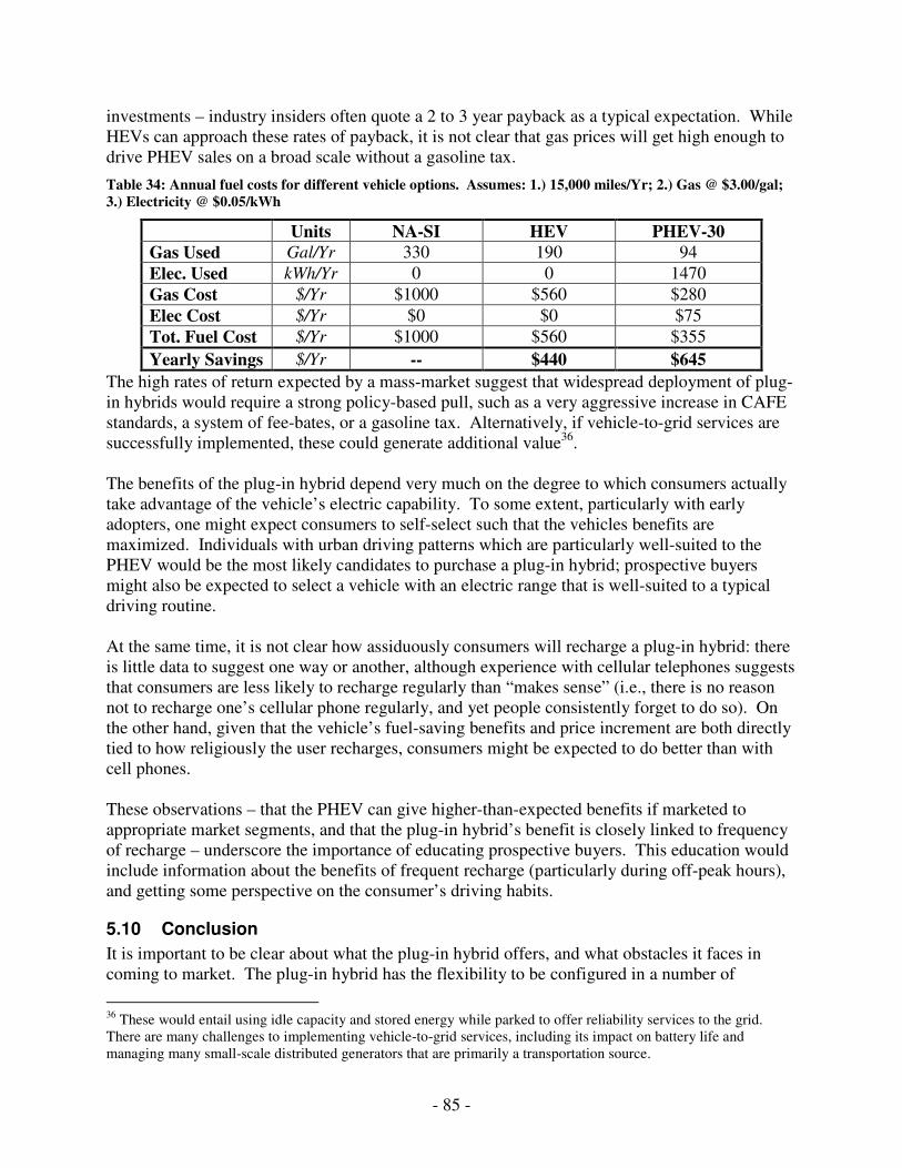
- 85 -

investments – industry insiders often quote a 2 to 3 year payback as a typical expectation. While HEVs can approach these rates of payback, it is not clear that gas prices will get high enough to drive PHEV sales on a broad scale without a gasoline tax.

Table 34: Annual fuel costs for different vehicle options. Assumes: 1.) 15,000 miles/Yr; 2.) Gas @ $3.00/gal; 3.) Electricity @ $0.05/kWh

Units NA-SI HEV PHEV-30 Gas Used Gal/Yr 330 190 94

Elec. Used kWh/Yr 0 0 1470

Gas Cost $/Yr $1000 $560 $280

Elec Cost $/Yr $0 $0 $75

Tot. Fuel Cost $/Yr $1000 $560 $355

Yearly Savings $/Yr -- $440 $645

The high rates of return expected by a mass-market suggest that widespread deployment of plug-in hybrids would require a strong policy-based pull, such as a very aggressive increase in CAFE standards, a system of fee-bates, or a gasoline tax. Alternatively, if vehicle-to-grid services are successfully implemented, these could generate additional value36. The benefits of the plug-in hybrid depend very much on the degree to which consumers actually take advantage of the vehicle’s electric capability. To some extent, particularly with early adopters, one might expect consumers to self-select such that the vehicles benefits are maximized. Individuals with urban driving patterns which are particularly well-suited to the PHEV would be the most likely candidates to purchase a plug-in hybrid; prospective buyers might also be expected to select a vehicle with an electric range that is well-suited to a typical driving routine. At the same time, it is not clear how assiduously consumers will recharge a plug-in hybrid: there is little data to suggest one way or another, although experience with cellular telephones suggests that consumers are less likely to recharge regularly than “makes sense” (i.e., there is no reason not to recharge one’s cellular phone regularly, and yet people consistently forget to do so). On the other hand, given that the vehicle’s fuel-saving benefits and price increment are both directly tied to how religiously the user recharges, consumers might be expected to do better than with cell phones. These observations – that the PHEV can give higher-than-expected benefits if marketed to appropriate market segments, and that the plug-in hybrid’s benefit is closely linked to frequency of recharge – underscore the importance of educating prospective buyers. This education would include information about the benefits of frequent recharge (particularly during off-peak hours), and getting some perspective on the consumer’s driving habits.

5.10 Conclusion

It is important to be clear about what the plug-in hybrid offers, and what obstacles it faces in coming to market. The plug-in hybrid has the flexibility to be configured in a number of

36 These would entail using idle capacity and stored energy while parked to offer reliability services to the grid. There are many challenges to implementing vehicle-to-grid services, including its impact on battery life and managing many small-scale distributed generators that are primarily a transportation source.

- 86 -

different ways to optimize between cost, performance, and petroleum reduction. ADVISOR vehicle simulations indicate that blended-mode operation offers close to the petroleum reduction benefit of all-electric operation, but could be implemented more cheaply and offer performance benefits. There are advantages and disadvantages to both higher and lower electrical range vehicles. While the high cost of batteries and diminishing returns on petroleum savings will push the market towards lower electric range, vehicles with a higher electric range offer greater petroleum reduction benefits at decreasing marginal cost. In addition, vehicles with lower electric range impose a more strenuous duty cycle on the battery. This is because it requires more deep-discharge cycles, higher discharge during charge-sustaining operation, and must operate at higher amperage. Given that there is no optimum electric range, a plug-in hybrid with a 30-mile range (PHEV-30) is used as the base case. Vehicle simulations and a review of typical driving patterns showed that the plug-in hybrid offers significant petroleum-reduction benefits, even at relatively low electric range: for example, the PHEV-30 uses roughly one-third the petroleum of the NA-SI baseline, and one-half that of the HEV. Depending on how the electric grid evolves, the plug-in hybrid can offer CO2 benefits. A plug-in hybrid charging off of the base case electric grid projection offers nearly the same GHG-reduction benefits as the hybrid vehicle. If the grid tends towards an increasing fraction of natural gas or non GHG-emitting generators, the plug-in hybrid becomes a much more attractive GHG reduction opportunity. Conversely, if coal (without CCS) becomes more dominant, grid-charged vehicles will increase GHG emissions. The primary technical challenge in bringing the plug-in hybrid to market is the development of a lithium-ion battery that lasts the life of the vehicle and a willingness on the part of manufacturers to warranty this battery. There are also questions as to how to integrate engine and motor operation during blended mode driving, but this is a secondary challenge. Beyond these vehicle design issues, the plug-in hybrid must overcome several additional hurdles in delivering benefit to a mass-market. The primary challenge is cost-related: it is unlikely that market forces alone can drive widespread adoption. In addition, deployment of plug-in hybrids would be most beneficial from a societal standpoint if accompanied by measures that proactively encourage off-peak charging (for example, through dynamic pricing of electricity) and educating consumers on the benefits of frequently recharging the vehicle. On balance, these non-cost institutional and implementation barriers are relatively benign given the potential petroleum reduction benefits. In fact, this low infrastructure hurdle is a key selling point of the plug-in hybrid. In the near-term, the plug-in hybrid does not compete with the hybrid vehicle unless reducing petroleum consumption becomes an overriding concern. Over the longer-term, it has the potential to go beyond the capability of the hybrid in terms of both petroleum and GHG reductions. Its potential with respect to the fuel-cell and battery-electric vehicle will be discussed in the results portion of this paper.

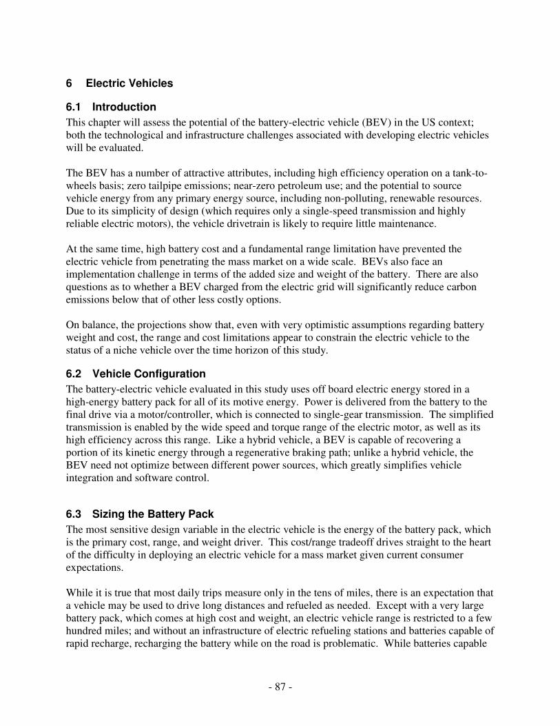
- 87 -

6 Electric Vehicles

6.1 Introduction

This chapter will assess the potential of the battery-electric vehicle (BEV) in the US context; both the technological and infrastructure challenges associated with developing electric vehicles will be evaluated. The BEV has a number of attractive attributes, including high efficiency operation on a tank-to-wheels basis; zero tailpipe emissions; near-zero petroleum use; and the potential to source vehicle energy from any primary energy source, including non-polluting, renewable resources. Due to its simplicity of design (which requires only a single-speed transmission and highly reliable electric motors), the vehicle drivetrain is likely to require little maintenance. At the same time, high battery cost and a fundamental range limitation have prevented the electric vehicle from penetrating the mass market on a wide scale. BEVs also face an implementation challenge in terms of the added size and weight of the battery. There are also questions as to whether a BEV charged from the electric grid will significantly reduce carbon emissions below that of other less costly options. On balance, the projections show that, even with very optimistic assumptions regarding battery weight and cost, the range and cost limitations appear to constrain the electric vehicle to the status of a niche vehicle over the time horizon of this study.

6.2 Vehicle Configuration

The battery-electric vehicle evaluated in this study uses off board electric energy stored in a high-energy battery pack for all of its motive energy. Power is delivered from the battery to the final drive via a motor/controller, which is connected to single-gear transmission. The simplified transmission is enabled by the wide speed and torque range of the electric motor, as well as its high efficiency across this range. Like a hybrid vehicle, a BEV is capable of recovering a portion of its kinetic energy through a regenerative braking path; unlike a hybrid vehicle, the BEV need not optimize between different power sources, which greatly simplifies vehicle integration and software control.

6.3 Sizing the Battery Pack

The most sensitive design variable in the electric vehicle is the energy of the battery pack, which is the primary cost, range, and weight driver. This cost/range tradeoff drives straight to the heart of the difficulty in deploying an electric vehicle for a mass market given current consumer expectations. While it is true that most daily trips measure only in the tens of miles, there is an expectation that a vehicle may be used to drive long distances and refueled as needed. Except with a very large battery pack, which comes at high cost and weight, an electric vehicle range is restricted to a few hundred miles; and without an infrastructure of electric refueling stations and batteries capable of rapid recharge, recharging the battery while on the road is problematic. While batteries capable

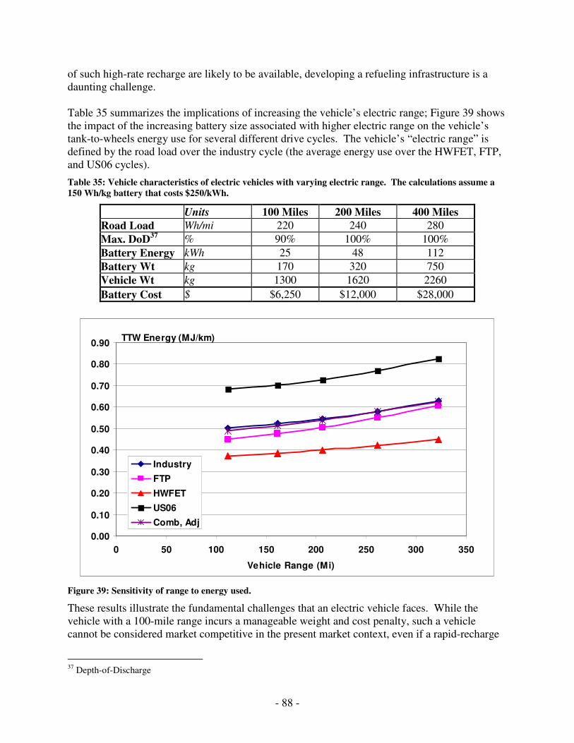
- 88 -

of such high-rate recharge are likely to be available, developing a refueling infrastructure is a daunting challenge. Table 35 summarizes the implications of increasing the vehicle’s electric range; Figure 39 shows the impact of the increasing battery size associated with higher electric range on the vehicle’s tank-to-wheels energy use for several different drive cycles. The vehicle’s “electric range” is defined by the road load over the industry cycle (the average energy use over the HWFET, FTP, and US06 cycles).

Table 35: Vehicle characteristics of electric vehicles with varying electric range. The calculations assume a 150 Wh/kg battery that costs $250/kWh.

Units 100 Miles 200 Miles 400 Miles

Road Load Wh/mi 220 240 280

Max. DoD37 % 90% 100% 100%

Battery Energy kWh 25 48 112

Battery Wt kg 170 320 750

Vehicle Wt kg 1300 1620 2260

Battery Cost $ $6,250 $12,000 $28,000

TTW Energy (MJ/km)

0.00

0.10

0.20

0.30

0.40

0.50

0.60

0.70

0.80

0.90

0 50 100 150 200 250 300 350

Vehicle Range (Mi)

Industry

FTP

HWFET

US06

Comb, Adj

Figure 39: Sensitivity of range to energy used.

These results illustrate the fundamental challenges that an electric vehicle faces. While the vehicle with a 100-mile range incurs a manageable weight and cost penalty, such a vehicle cannot be considered market competitive in the present market context, even if a rapid-recharge

37 Depth-of-Discharge

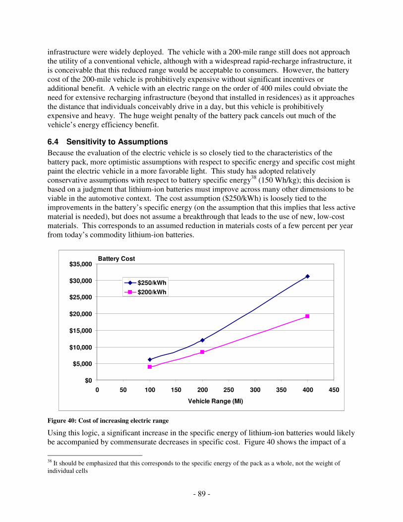
- 89 -

infrastructure were widely deployed. The vehicle with a 200-mile range still does not approach the utility of a conventional vehicle, although with a widespread rapid-recharge infrastructure, it is conceivable that this reduced range would be acceptable to consumers. However, the battery cost of the 200-mile vehicle is prohibitively expensive without significant incentives or additional benefit. A vehicle with an electric range on the order of 400 miles could obviate the need for extensive recharging infrastructure (beyond that installed in residences) as it approaches the distance that individuals conceivably drive in a day, but this vehicle is prohibitively expensive and heavy. The huge weight penalty of the battery pack cancels out much of the vehicle’s energy efficiency benefit.

6.4 Sensitivity to Assumptions

Because the evaluation of the electric vehicle is so closely tied to the characteristics of the battery pack, more optimistic assumptions with respect to specific energy and specific cost might paint the electric vehicle in a more favorable light. This study has adopted relatively conservative assumptions with respect to battery specific energy38 (150 Wh/kg); this decision is based on a judgment that lithium-ion batteries must improve across many other dimensions to be viable in the automotive context. The cost assumption ($250/kWh) is loosely tied to the improvements in the battery’s specific energy (on the assumption that this implies that less active material is needed), but does not assume a breakthrough that leads to the use of new, low-cost materials. This corresponds to an assumed reduction in materials costs of a few percent per year from today’s commodity lithium-ion batteries.

Battery Cost

$0

$5,000

$10,000

$15,000

$20,000

$25,000

$30,000

$35,000

0 50 100 150 200 250 300 350 400 450

Vehicle Range (Mi)

$250/kWh

$200/kWh

Figure 40: Cost of increasing electric range

Using this logic, a significant increase in the specific energy of lithium-ion batteries would likely be accompanied by commensurate decreases in specific cost. Figure 40 shows the impact of a

38 It should be emphasized that this corresponds to the specific energy of the pack as a whole, not the weight of individual cells

- 90 -

more optimistic assumption; in this case, battery costs are assumed to be $200/kWh compared to the $250/kWh baseline. Under these conditions, the vehicle with a 400-mile range continues to remain prohibitively expensive, with battery costs of $19,000. However, the 200-mile vehicle becomes more attractive, with a battery cost of only $8,400. Note that this optimistic case not only lessens the battery cost on a unit basis, but it enables the vehicle to use fewer batteries due to the higher specific energy. Table 36 compares a more optimistic version of the 200-mile electric vehicle with the base case. The optimistic case uses the $200/kWh cost assumption, as well as a very optimistic (but not implausible) battery weight characteristic of 300 Wh/kg. The reduction in battery weight accounts for a 13% decrease in the vehicle load.

Table 36: Sensitivity of the 200-mile electric vehicle to the assumed battery characteristics

Units Baseline: 150 Wh/kg, $250/kWh

Optimistic: 300 Wh/kg, $200/kWh

Range Mi 200 200

Vehicle Load Wh/mi 240 210

Battery Energy kWh 48 42

Battery Wt kg 320 160

Vehicle Wt kg 1620 1360

Battery Cost $ $12,000 $8,400

With these optimistic assumptions, the vehicle with a 200-mile range is a more viable option, though still quite expensive, with an estimated incremental cost of $6,900 more than the baseline NA-SI vehicle (compared to $10,200 for the base case) (see Table 53 for cost projections). However, it must be emphasized that these battery improvements would also show up in decreased cost for the plug-in hybrid and conventional hybrid vehicles.

6.5 Conclusion

Selling an electric vehicle to a mass-market is a particularly difficult challenge because the vehicle will be range limited and will be more expensive than other vehicle options. Even with optimistic assumptions about battery cost and weight, the electric vehicle is quite expensive and continues to be range-limited. In addition, the electric vehicle would require a recharge infrastructure, and may require upgrades to residential outlets. It is worth noting that, over the long run, the shortcomings of the electric vehicle are almost entirely a function of the cost/range tradeoff. In particular, battery recharge rates are not at issue (the speed of recharge is more likely to be constrained by recharge infrastructure than battery rate limitations); nor is battery performance (with respect to efficiency, lifetime, safety, or even weight). The combination of high cost and limited range are likely to persist over the time horizon of this study. As such, unless there is a dramatic shift in consumer expectations, the electric vehicle is likely to remain a niche vehicle.

- 91 -

7 Fuel-Cell Vehicles

Hydrogen-powered fuel cell vehicles (FCVs) have attracted a great deal of attention as a possible replacement for the internal combustion engine. An FCV offers a number of attractive properties over other options. Hydrogen may be produced using a variety of energy sources, enabling diversification of the transportation system away from its near-total reliance on petroleum. Because the only reaction by-product is water, a fuel-cell vehicle produces near-zero tailpipe emissions. If the fuel (hydrogen) is produced from non-GHG emitting sources, an FCV is capable of near-zero well-to-wheel emissions. A fuel cell also offers very high theoretical efficiency. An actual hydrogen-based automotive fuel cell transportation system introduces a number of practical constraints to this ideal model. At the stack level, fuel cell performance and durability is limited by the properties of present-day membrane materials, catalyst properties, and system management, and current systems are very expensive with powerplant costs for high volume production projected to be a factor of 3 more expensive than a spark-ignition engine. At the vehicle level, storing enough hydrogen (which has low volumetric energy density) to allow for adequate vehicle range is problematic. And at the level of the transportation system, it is not clear how to transition to a hydrogen infrastructure; nor will hydrogen deliver the promised near-zero well-to-wheel emissions if produced from natural gas without carbon capture. This chapter will assess the well-to-wheel energy use and greenhouse gas emissions of a 2030 fuel-cell vehicle. Tank-to-wheels characteristics are estimated by projecting the performance characteristics of a future fuel-cell stack and integrating them into a vehicle software model in ADVISOR. Well-to-tank energy and greenhouse-gas emissions are estimated using published data for a gaseous hydrogen fueling infrastructure. Other factors, such as range and durability, are assessed by reviewing the available literature, and in the case of range, feeding the appropriate data into the vehicle model. Cost is assessed using the cost model previously developed by Tiax as part of the ongoing Department of Energy (DOE) fuel-cell review[Carlson 2005]. To maintain consistency with the projected performance, appropriate parameters are adjusted. Key Questions to be addressed include:

1.) Can fuel cells meet automotive durability and reliability requirements? 2.) How much are fuel cell and hydrogen storage costs likely to decrease? What advances

need to happen to approach achieve price-parity with conventional vehicles? 3.) What factors dictate the vehicle’s degree of hybridization? How sensitive is energy use

to this parameter? 4.) What is the CO2 impact of a hydrogen-fueled transportation system? 5.) What is the status of onboard hydrogen storage technology, and what are the implications

with respect to range? 6.) What developments or breakthroughs are needed for fuel-cell vehicles to become market

and cost competitive?

- 92 -

7.1 Vehicle

7.1.1 Overview

Figure 41: A series-hybrid fuel-cell vehicle architecture. Arrows show possible power flows: The fuel-cell converts hydrogen to electricity, which is used to either deliver traction power to the motor or to charge the battery; a portion of the vehicle’s kinetic energy may be recovered through regenerative braking.

The 2030 fuel-cell vehicle (FCV) (Figure 41) is assumed to use a proton-exchange membrane (PEM) fuel-cell system to power a motor in a series hybrid configuration. The motor is a scaled version of the DC permanent-magnet motor used for the gasoline hybrid-electric vehicle, sized to meet vehicle performance requirements. The vehicle is fueled directly by a gaseous hydrogen fuel tank. Hybridizing the vehicle entails down-sizing the fuel-cell while integrating a high-power energy storage system to respond to transient power requests. The vehicle is assumed to use a high-power lithium-ion battery, although either ultracapacitors or nickel-metal hydride batteries might also be suitable for a fuel-cell hybrid. Differences in performance and efficiency between these different energy storage options are negligible; this choice will likely be based on other factors such as cost, durability, and packaging. Hybridizing the vehicle is advantageous for a number of reasons:

1.) Batteries are likely to be cheaper and lighter, on a per-kW basis, than a fuel-cell. 2.) A smaller fuel-cell lessens the heat rejection requirement. Due to membrane

requirements, the fuel-cell operating temperature cannot go much above 80 C; rejecting heat at such a low temperature is non-trivial.

3.) It increases the vehicle’s on-road efficiency, both by enabling regenerative braking and by operating the fuel cell at the high-efficiency points on its operating curve.

4.) From an operations perspective, it simplifies start-up (depending on ambient temperatures, a fuel-cell may take several minutes to achieve full power operation).

5.) It may enable reductions in the size of the balance-of-plant by lessening the fuel-cell’s transient response requirement (i.e., the fuel-cell’s load-following capability) [Ahluwalia 2005].

The vehicle simulations presented in the Results section will test several different levels of hybridization to determine the sensitivity of TTW energy use on degree-of-hybridization.

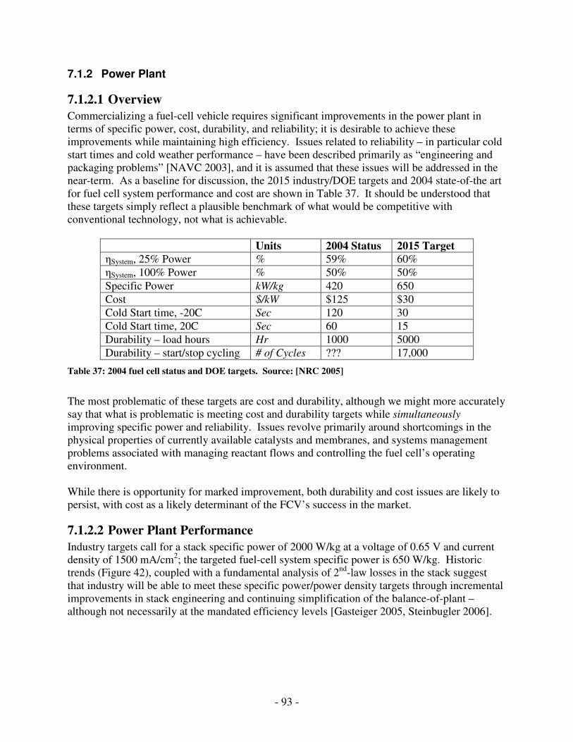
- 93 -

7.1.2 Power Plant

7.1.2.1 Overview

Commercializing a fuel-cell vehicle requires significant improvements in the power plant in terms of specific power, cost, durability, and reliability; it is desirable to achieve these improvements while maintaining high efficiency. Issues related to reliability – in particular cold start times and cold weather performance – have been described primarily as “engineering and packaging problems” [NAVC 2003], and it is assumed that these issues will be addressed in the near-term. As a baseline for discussion, the 2015 industry/DOE targets and 2004 state-of-the art for fuel cell system performance and cost are shown in Table 37. It should be understood that these targets simply reflect a plausible benchmark of what would be competitive with conventional technology, not what is achievable.

Units 2004 Status 2015 Target ηSystem, 25% Power % 59% 60%

ηSystem, 100% Power % 50% 50%

Specific Power kW/kg 420 650

Cost $/kW $125 $30

Cold Start time, -20C Sec 120 30

Cold Start time, 20C Sec 60 15

Durability – load hours Hr 1000 5000

Durability – start/stop cycling # of Cycles ??? 17,000

Table 37: 2004 fuel cell status and DOE targets. Source: [NRC 2005]

The most problematic of these targets are cost and durability, although we might more accurately say that what is problematic is meeting cost and durability targets while simultaneously improving specific power and reliability. Issues revolve primarily around shortcomings in the physical properties of currently available catalysts and membranes, and systems management problems associated with managing reactant flows and controlling the fuel cell’s operating environment. While there is opportunity for marked improvement, both durability and cost issues are likely to persist, with cost as a likely determinant of the FCV’s success in the market.

7.1.2.2 Power Plant Performance

Industry targets call for a stack specific power of 2000 W/kg at a voltage of 0.65 V and current density of 1500 mA/cm2; the targeted fuel-cell system specific power is 650 W/kg. Historic trends (Figure 42), coupled with a fundamental analysis of 2nd-law losses in the stack suggest that industry will be able to meet these specific power/power density targets through incremental improvements in stack engineering and continuing simplification of the balance-of-plant – although not necessarily at the mandated efficiency levels [Gasteiger 2005, Steinbugler 2006].

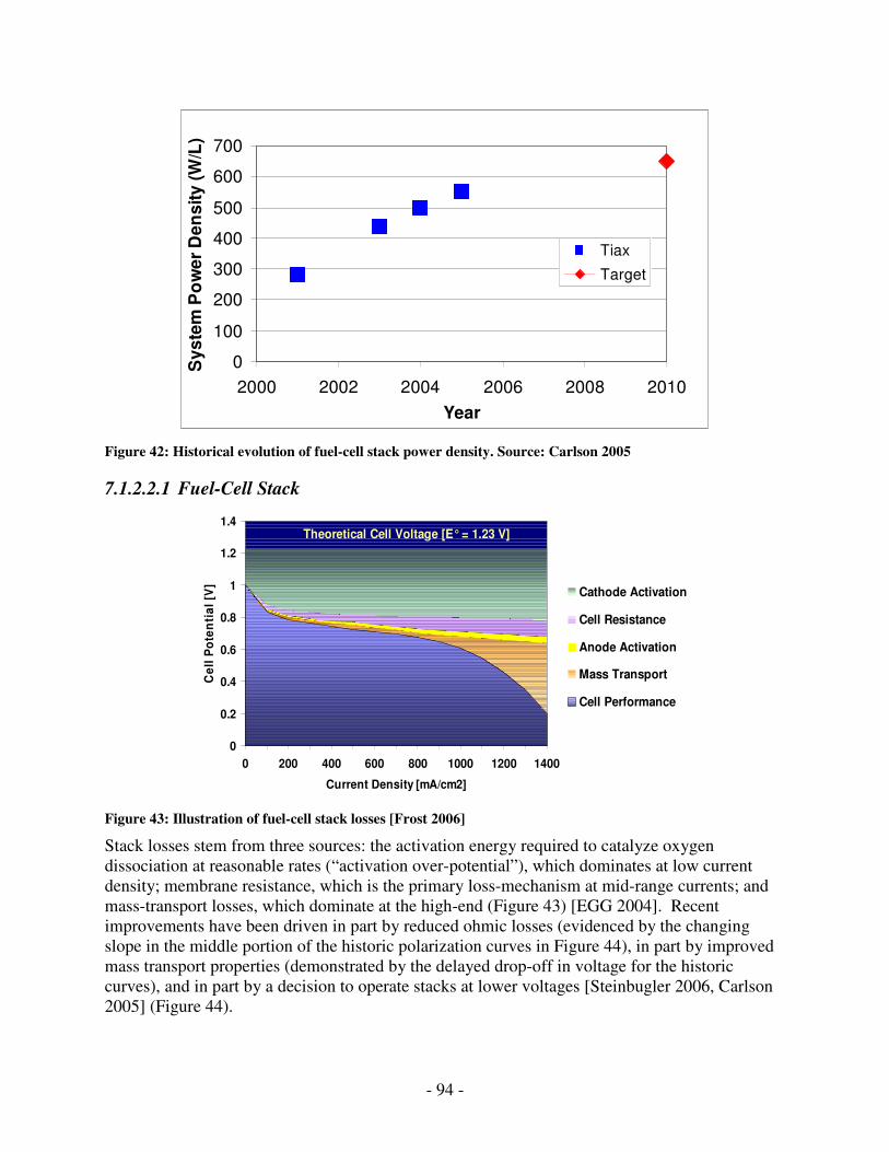
- 94 -

0

100

200

300

400

500

600

700

2000 2002 2004 2006 2008 2010

Year

Sy

ste

m P

ow

er

De

ns

ity

(W

/L)

Tiax

Target

Figure 42: Historical evolution of fuel-cell stack power density. Source: Carlson 2005

7.1.2.2.1 Fuel-Cell Stack

Figure 43: Illustration of fuel-cell stack losses [Frost 2006]

Stack losses stem from three sources: the activation energy required to catalyze oxygen dissociation at reasonable rates (“activation over-potential”), which dominates at low current density; membrane resistance, which is the primary loss-mechanism at mid-range currents; and mass-transport losses, which dominate at the high-end (Figure 43) [EGG 2004]. Recent improvements have been driven in part by reduced ohmic losses (evidenced by the changing slope in the middle portion of the historic polarization curves in Figure 44), in part by improved mass transport properties (demonstrated by the delayed drop-off in voltage for the historic curves), and in part by a decision to operate stacks at lower voltages [Steinbugler 2006, Carlson 2005] (Figure 44).

0

0.2

0.4

0.6

0.8

1

1.2

1.4

0 200 400 600 800 1000 1200 1400

Current Density [mA/cm2]

Ce

ll P

ote

nti

al

[V]

Cathode Activation

Cell Resistance

Anode Activation

Mass Transport

Cell Performance

Theoretical Cell Voltage [E° = 1.23 V]

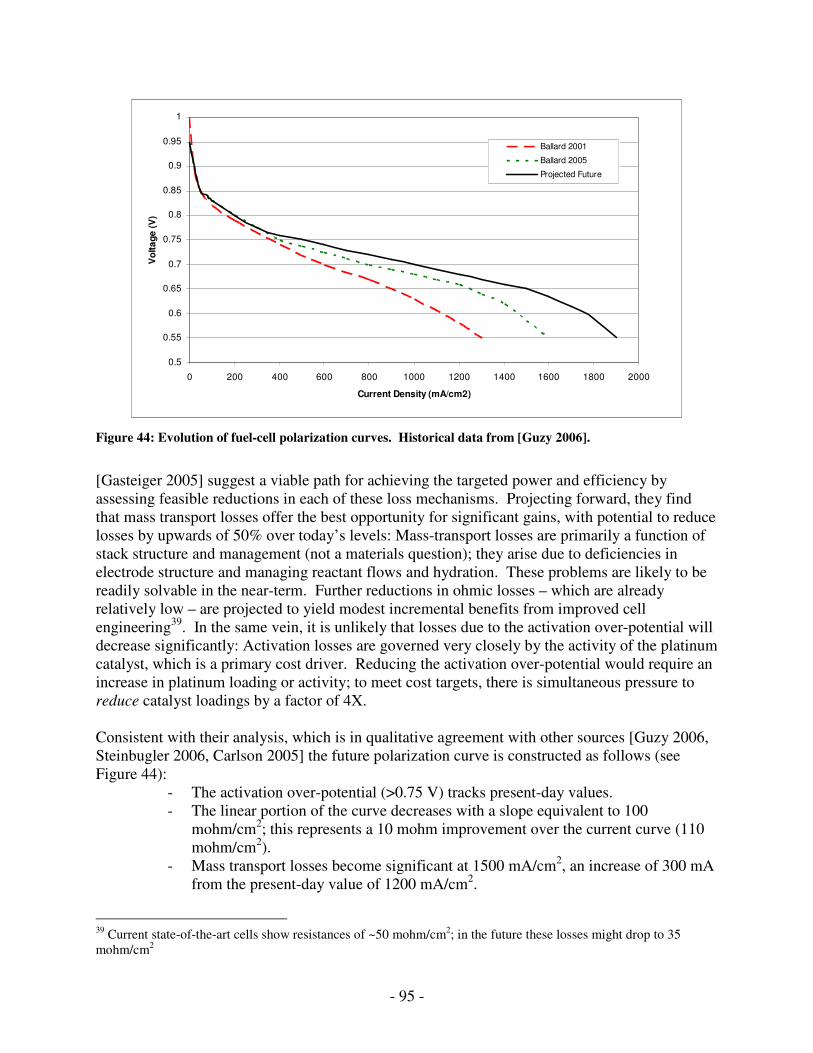
- 95 -

0.5

0.55

0.6

0.65

0.7

0.75

0.8

0.85

0.9

0.95

1

0 200 400 600 800 1000 1200 1400 1600 1800 2000

Current Density (mA/cm2)

Vo

lta

ge

(V

)Ballard 2001

Ballard 2005

Projected Future

Figure 44: Evolution of fuel-cell polarization curves. Historical data from [Guzy 2006].

[Gasteiger 2005] suggest a viable path for achieving the targeted power and efficiency by assessing feasible reductions in each of these loss mechanisms. Projecting forward, they find that mass transport losses offer the best opportunity for significant gains, with potential to reduce losses by upwards of 50% over today’s levels: Mass-transport losses are primarily a function of stack structure and management (not a materials question); they arise due to deficiencies in electrode structure and managing reactant flows and hydration. These problems are likely to be readily solvable in the near-term. Further reductions in ohmic losses – which are already relatively low – are projected to yield modest incremental benefits from improved cell engineering39. In the same vein, it is unlikely that losses due to the activation over-potential will decrease significantly: Activation losses are governed very closely by the activity of the platinum catalyst, which is a primary cost driver. Reducing the activation over-potential would require an increase in platinum loading or activity; to meet cost targets, there is simultaneous pressure to reduce catalyst loadings by a factor of 4X. Consistent with their analysis, which is in qualitative agreement with other sources [Guzy 2006, Steinbugler 2006, Carlson 2005] the future polarization curve is constructed as follows (see Figure 44):

- The activation over-potential (>0.75 V) tracks present-day values. - The linear portion of the curve decreases with a slope equivalent to 100

mohm/cm2; this represents a 10 mohm improvement over the current curve (110 mohm/cm2).

- Mass transport losses become significant at 1500 mA/cm2, an increase of 300 mA from the present-day value of 1200 mA/cm2.

39 Current state-of-the-art cells show resistances of ~50 mohm/cm2; in the future these losses might drop to 35 mohm/cm2

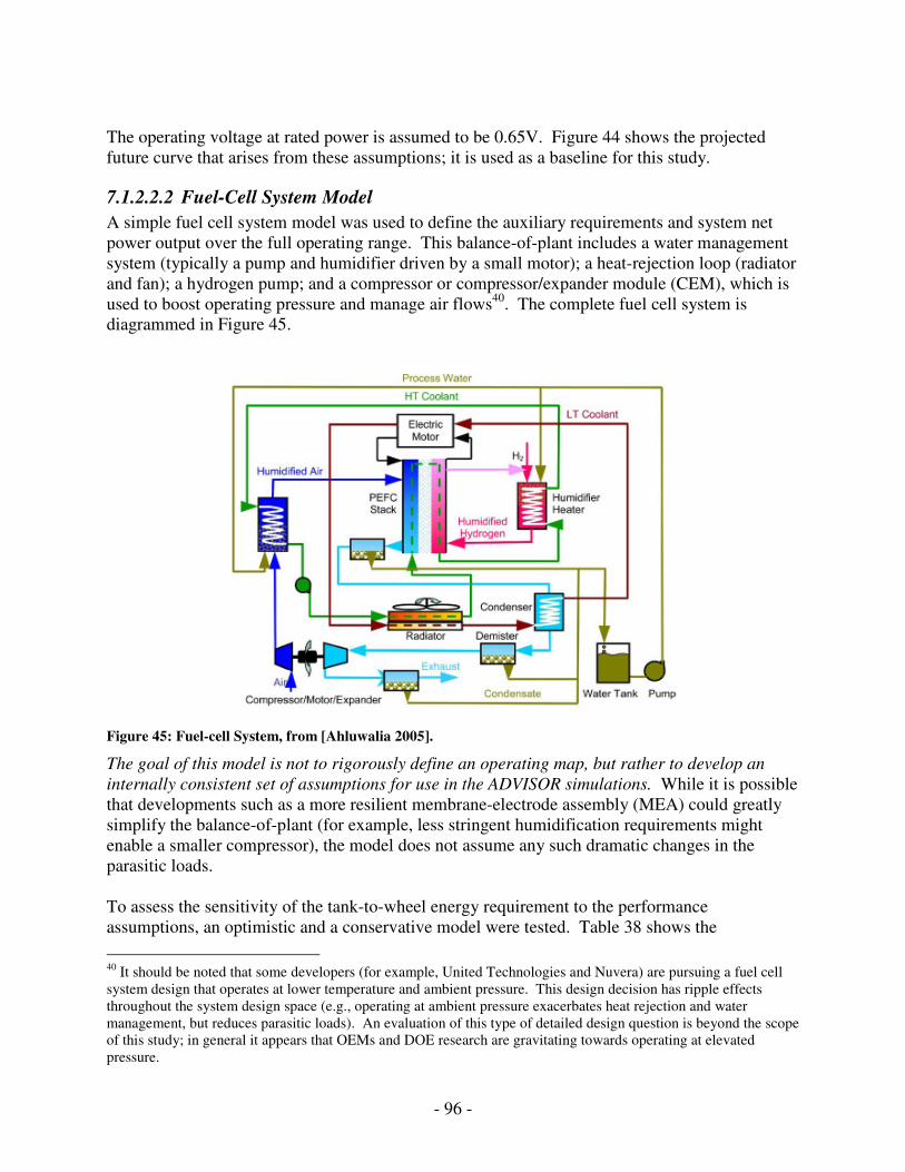
- 96 -

The operating voltage at rated power is assumed to be 0.65V. Figure 44 shows the projected future curve that arises from these assumptions; it is used as a baseline for this study.

7.1.2.2.2 Fuel-Cell System Model

A simple fuel cell system model was used to define the auxiliary requirements and system net power output over the full operating range. This balance-of-plant includes a water management system (typically a pump and humidifier driven by a small motor); a heat-rejection loop (radiator and fan); a hydrogen pump; and a compressor or compressor/expander module (CEM), which is used to boost operating pressure and manage air flows40. The complete fuel cell system is diagrammed in Figure 45.

Figure 45: Fuel-cell System, from [Ahluwalia 2005].

The goal of this model is not to rigorously define an operating map, but rather to develop an internally consistent set of assumptions for use in the ADVISOR simulations. While it is possible that developments such as a more resilient membrane-electrode assembly (MEA) could greatly simplify the balance-of-plant (for example, less stringent humidification requirements might enable a smaller compressor), the model does not assume any such dramatic changes in the parasitic loads. To assess the sensitivity of the tank-to-wheel energy requirement to the performance assumptions, an optimistic and a conservative model were tested. Table 38 shows the

40 It should be noted that some developers (for example, United Technologies and Nuvera) are pursuing a fuel cell system design that operates at lower temperature and ambient pressure. This design decision has ripple effects throughout the system design space (e.g., operating at ambient pressure exacerbates heat rejection and water management, but reduces parasitic loads). An evaluation of this type of detailed design question is beyond the scope of this study; in general it appears that OEMs and DOE research are gravitating towards operating at elevated pressure.

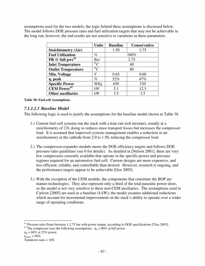
- 97 -

assumptions used for the two models; the logic behind these assumptions is discussed below. The model follows DOE pressure ratio and fuel utilization targets that may not be achievable in the long run; however, the end results are not sensitive to variations in these parameters.

Units Baseline Conservative Stoichiometry (Air) 1.50 1.75

Fuel Utilization % 100%

PR @ full pwr41 Bar 2.75

Inlet Temperature OC 40

Outlet Temperature OC 80

Min. Voltage V 0.65 0.60

η, peak % 52% 47%

Specific Power W/kg 650 520

CEM Power42 kW 5.1 12.3

Other auxiliaries kW 3.5 3.5

Table 38: Fuel-cell Assumptions

7.1.2.2.3 Baseline Model

The following logic is used to justify the assumptions for the baseline model shown in Table 38.

1.) Current fuel-cell systems run the stack with a lean (air-rich mixture), usually at a stoichiometry of 2.0; doing so reduces mass transport losses but increases the compressor load. It is assumed that improved systems management enables a reduction in air stoichiometry at the cathode from 2.0 to 1.50, reducing the compressor load.

2.) The compressor-expander module meets the DOE efficiency targets and follows DOE

pressure-ratio guidelines (see 0 for details). As detailed in [Nelson 2001], there are very few compressors currently available that operate in the specific power and pressure regimes required for an automotive fuel-cell. Current designs are more expensive, and less efficient, reliable, and controllable than desired. However, research is ongoing, and the performance targets appear to be achievable [Gee 2005].

3.) With the exception of the CEM module, the components that constitute the BOP are

mature technologies. They also represent only a third of the total parasitic power draw, so the model is not very sensitive to these non-CEM auxiliaries. The assumptions used in Carlson [2005] are used as a baseline (4 kW); the model assumes additional reductions which account for incremental improvements in the stack’s ability to operate over a wider range of operating conditions.

41 Pressure ratio floats between 1-2.75 bar with power output, according to DOE specifications [Tiax 2003]. 42 The compressor uses the following assumptions: ηIs = 80% at full power ηIs = 60% at 25% power ηmotor = 90% Turndown ratio = 10X

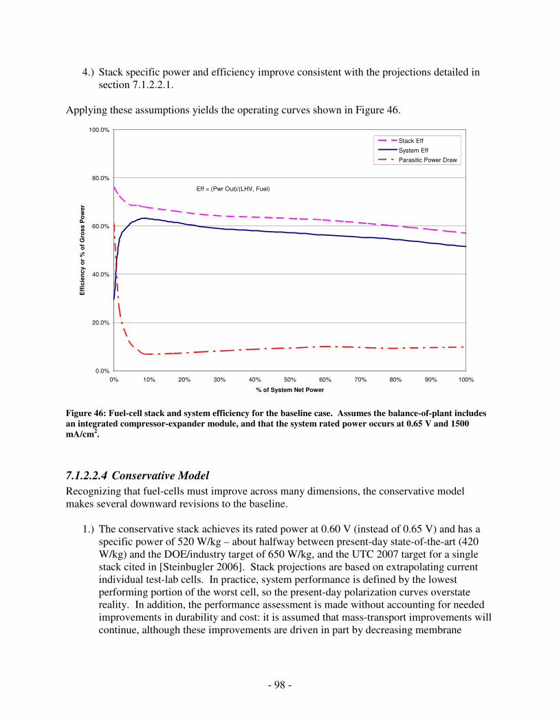
- 98 -

4.) Stack specific power and efficiency improve consistent with the projections detailed in section 7.1.2.2.1.

Applying these assumptions yields the operating curves shown in Figure 46.

0.0%

20.0%

40.0%

60.0%

80.0%

100.0%

0% 10% 20% 30% 40% 50% 60% 70% 80% 90% 100%

% of System Net Power

Eff

icie

nc

y o

r %

of

Gro

ss

Po

wer

Stack Eff

System Eff

Parasitic Power Draw

Eff = (Pwr Out)/(LHV, Fuel)

Figure 46: Fuel-cell stack and system efficiency for the baseline case. Assumes the balance-of-plant includes an integrated compressor-expander module, and that the system rated power occurs at 0.65 V and 1500 mA/cm2.

7.1.2.2.4 Conservative Model

Recognizing that fuel-cells must improve across many dimensions, the conservative model makes several downward revisions to the baseline.

1.) The conservative stack achieves its rated power at 0.60 V (instead of 0.65 V) and has a specific power of 520 W/kg – about halfway between present-day state-of-the-art (420 W/kg) and the DOE/industry target of 650 W/kg, and the UTC 2007 target for a single stack cited in [Steinbugler 2006]. Stack projections are based on extrapolating current individual test-lab cells. In practice, system performance is defined by the lowest performing portion of the worst cell, so the present-day polarization curves overstate reality. In addition, the performance assessment is made without accounting for needed improvements in durability and cost: it is assumed that mass-transport improvements will continue, although these improvements are driven in part by decreasing membrane

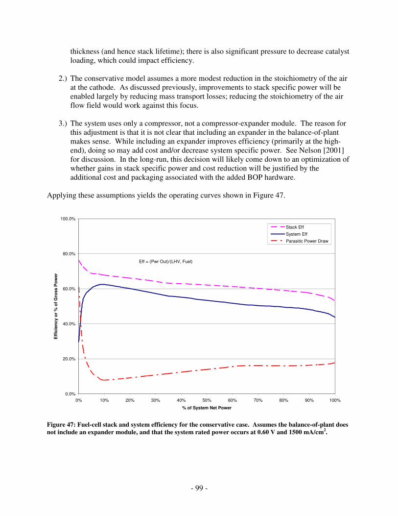
- 99 -

thickness (and hence stack lifetime); there is also significant pressure to decrease catalyst loading, which could impact efficiency.

2.) The conservative model assumes a more modest reduction in the stoichiometry of the air

at the cathode. As discussed previously, improvements to stack specific power will be enabled largely by reducing mass transport losses; reducing the stoichiometry of the air flow field would work against this focus.

3.) The system uses only a compressor, not a compressor-expander module. The reason for

this adjustment is that it is not clear that including an expander in the balance-of-plant makes sense. While including an expander improves efficiency (primarily at the high-end), doing so may add cost and/or decrease system specific power. See Nelson [2001] for discussion. In the long-run, this decision will likely come down to an optimization of whether gains in stack specific power and cost reduction will be justified by the additional cost and packaging associated with the added BOP hardware.

Applying these assumptions yields the operating curves shown in Figure 47.

0.0%

20.0%

40.0%

60.0%

80.0%

100.0%

0% 10% 20% 30% 40% 50% 60% 70% 80% 90% 100%

% of System Net Power

Eff

icie

nc

y o

r %

of

Gro

ss P

ow

er

Stack Eff

System Eff

Parasitic Power Draw

Eff = (Pwr Out)/(LHV, Fuel)

Figure 47: Fuel-cell stack and system efficiency for the conservative case. Assumes the balance-of-plant does not include an expander module, and that the system rated power occurs at 0.60 V and 1500 mA/cm2.

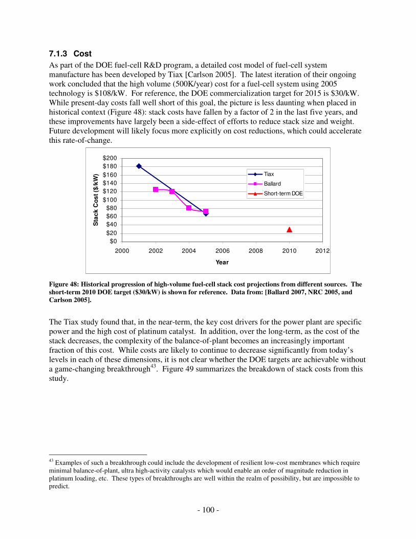
- 100 -

7.1.3 Cost

As part of the DOE fuel-cell R&D program, a detailed cost model of fuel-cell system manufacture has been developed by Tiax [Carlson 2005]. The latest iteration of their ongoing work concluded that the high volume (500K/year) cost for a fuel-cell system using 2005 technology is $108/kW. For reference, the DOE commercialization target for 2015 is $30/kW. While present-day costs fall well short of this goal, the picture is less daunting when placed in historical context (Figure 48): stack costs have fallen by a factor of 2 in the last five years, and these improvements have largely been a side-effect of efforts to reduce stack size and weight. Future development will likely focus more explicitly on cost reductions, which could accelerate this rate-of-change.

$0

$20

$40

$60

$80

$100

$120

$140

$160

$180

$200

2000 2002 2004 2006 2008 2010 2012

Year

Sta

ck

Co

st

($/k

W) Tiax

Ballard

Short-term DOE

Figure 48: Historical progression of high-volume fuel-cell stack cost projections from different sources. The short-term 2010 DOE target ($30/kW) is shown for reference. Data from: [Ballard 2007, NRC 2005, and Carlson 2005].

The Tiax study found that, in the near-term, the key cost drivers for the power plant are specific power and the high cost of platinum catalyst. In addition, over the long-term, as the cost of the stack decreases, the complexity of the balance-of-plant becomes an increasingly important fraction of this cost. While costs are likely to continue to decrease significantly from today’s levels in each of these dimensions, it is not clear whether the DOE targets are achievable without a game-changing breakthrough43. Figure 49 summarizes the breakdown of stack costs from this study.

43 Examples of such a breakthrough could include the development of resilient low-cost membranes which require minimal balance-of-plant, ultra high-activity catalysts which would enable an order of magnitude reduction in platinum loading, etc. These types of breakthroughs are well within the realm of possibility, but are impossible to predict.

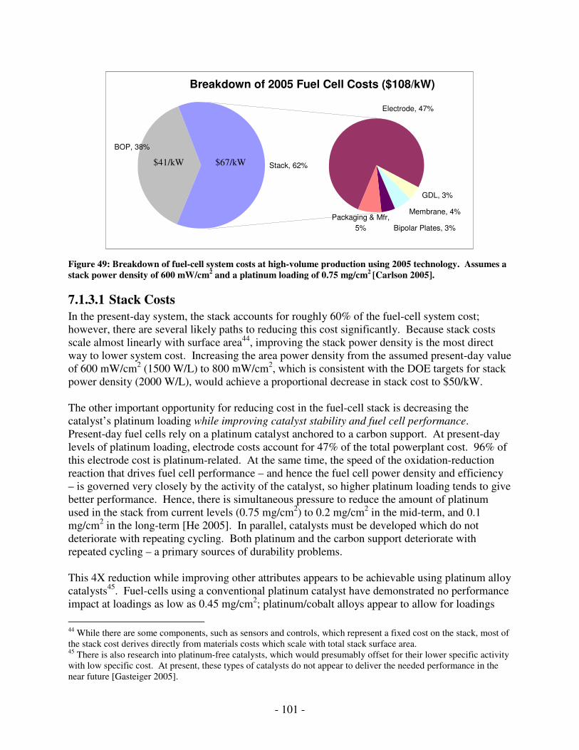
- 101 -

Figure 49: Breakdown of fuel-cell system costs at high-volume production using 2005 technology. Assumes a stack power density of 600 mW/cm2 and a platinum loading of 0.75 mg/cm2 [Carlson 2005].

7.1.3.1 Stack Costs

In the present-day system, the stack accounts for roughly 60% of the fuel-cell system cost; however, there are several likely paths to reducing this cost significantly. Because stack costs scale almost linearly with surface area44, improving the stack power density is the most direct way to lower system cost. Increasing the area power density from the assumed present-day value of 600 mW/cm2 (1500 W/L) to 800 mW/cm2, which is consistent with the DOE targets for stack power density (2000 W/L), would achieve a proportional decrease in stack cost to $50/kW. The other important opportunity for reducing cost in the fuel-cell stack is decreasing the catalyst’s platinum loading while improving catalyst stability and fuel cell performance. Present-day fuel cells rely on a platinum catalyst anchored to a carbon support. At present-day levels of platinum loading, electrode costs account for 47% of the total powerplant cost. 96% of this electrode cost is platinum-related. At the same time, the speed of the oxidation-reduction reaction that drives fuel cell performance – and hence the fuel cell power density and efficiency – is governed very closely by the activity of the catalyst, so higher platinum loading tends to give better performance. Hence, there is simultaneous pressure to reduce the amount of platinum used in the stack from current levels (0.75 mg/cm2) to 0.2 mg/cm2 in the mid-term, and 0.1 mg/cm2 in the long-term [He 2005]. In parallel, catalysts must be developed which do not deteriorate with repeating cycling. Both platinum and the carbon support deteriorate with repeated cycling – a primary sources of durability problems. This 4X reduction while improving other attributes appears to be achievable using platinum alloy catalysts45. Fuel-cells using a conventional platinum catalyst have demonstrated no performance impact at loadings as low as 0.45 mg/cm2; platinum/cobalt alloys appear to allow for loadings

44 While there are some components, such as sensors and controls, which represent a fixed cost on the stack, most of the stack cost derives directly from materials costs which scale with total stack surface area. 45 There is also research into platinum-free catalysts, which would presumably offset for their lower specific activity with low specific cost. At present, these types of catalysts do not appear to deliver the needed performance in the near future [Gasteiger 2005].

Breakdown of 2005 Fuel Cell Costs ($108/kW)

GDL, 3%

Bipolar Plates, 3%

Stack, 62%

Membrane, 4%

Electrode, 47%

BOP, 38%

Packaging & Mfr,

5%

$41/kW $67/kW

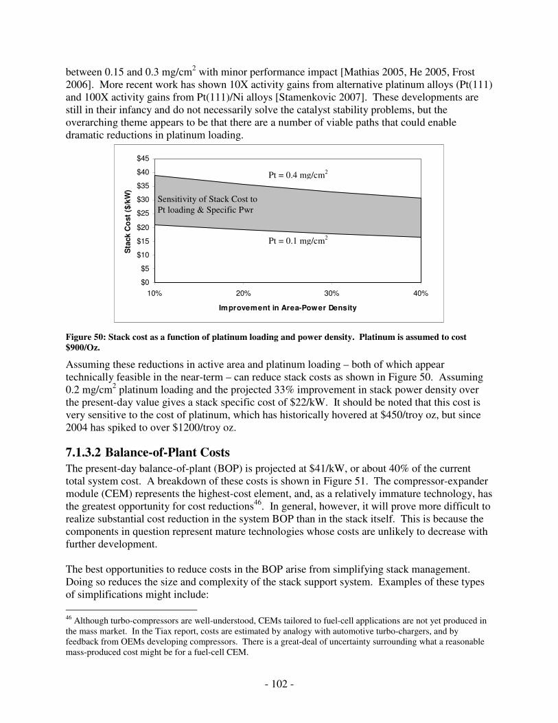
- 102 -

between 0.15 and 0.3 mg/cm2 with minor performance impact [Mathias 2005, He 2005, Frost 2006]. More recent work has shown 10X activity gains from alternative platinum alloys (Pt(111) and 100X activity gains from Pt(111)/Ni alloys [Stamenkovic 2007]. These developments are still in their infancy and do not necessarily solve the catalyst stability problems, but the overarching theme appears to be that there are a number of viable paths that could enable dramatic reductions in platinum loading.

$0

$5

$10

$15

$20

$25

$30

$35

$40

$45

10% 20% 30% 40%

Improvement in Area-Power Density

Sta

ck C

ost

($/k

W)

Figure 50: Stack cost as a function of platinum loading and power density. Platinum is assumed to cost $900/Oz.

Assuming these reductions in active area and platinum loading – both of which appear technically feasible in the near-term – can reduce stack costs as shown in Figure 50. Assuming 0.2 mg/cm2 platinum loading and the projected 33% improvement in stack power density over the present-day value gives a stack specific cost of $22/kW. It should be noted that this cost is very sensitive to the cost of platinum, which has historically hovered at $450/troy oz, but since 2004 has spiked to over $1200/troy oz.

7.1.3.2 Balance-of-Plant Costs

The present-day balance-of-plant (BOP) is projected at $41/kW, or about 40% of the current total system cost. A breakdown of these costs is shown in Figure 51. The compressor-expander module (CEM) represents the highest-cost element, and, as a relatively immature technology, has the greatest opportunity for cost reductions46. In general, however, it will prove more difficult to realize substantial cost reduction in the system BOP than in the stack itself. This is because the components in question represent mature technologies whose costs are unlikely to decrease with further development. The best opportunities to reduce costs in the BOP arise from simplifying stack management. Doing so reduces the size and complexity of the stack support system. Examples of these types of simplifications might include:

46 Although turbo-compressors are well-understood, CEMs tailored to fuel-cell applications are not yet produced in the mass market. In the Tiax report, costs are estimated by analogy with automotive turbo-chargers, and by feedback from OEMs developing compressors. There is a great-deal of uncertainty surrounding what a reasonable mass-produced cost might be for a fuel-cell CEM.

Pt = 0.1 mg/cm2

Sensitivity of Stack Cost to Pt loading & Specific Pwr

Pt = 0.4 mg/cm2

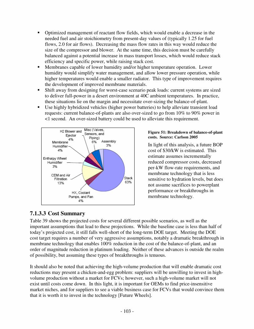
- 103 -

Optimized management of reactant flow fields, which would enable a decrease in the needed fuel and air stoichiometry from present-day values of (typically 1.25 for fuel flows, 2.0 for air flows). Decreasing the mass flow rates in this way would reduce the size of the compressor and blower. At the same time, this decision must be carefully balanced against a potential increase in mass transport losses, which would reduce stack efficiency and specific power, while raising stack cost.

Membranes capable of lower humidity and/or higher temperature operation. Lower humidity would simplify water management, and allow lower pressure operation, while higher temperatures would enable a smaller radiator. This type of improvement requires the development of improved membrane materials.

Shift away from designing for worst-case scenario peak loads: current systems are sized to deliver full-power in a desert environment at 40C ambient temperatures. In practice, these situations lie on the margin and necessitate over-sizing the balance-of-plant.

Use highly hybridized vehicles (higher power batteries) to help alleviate transient load requests: current balance-of-plants are also over-sized to go from 10% to 90% power in <1 second. An over-sized battery could be used to alleviate this requirement.

Figure 51: Breakdown of balance-of-plant costs. Source: Carlson 2005

In light of this analysis, a future BOP cost of $30/kW is estimated. This estimate assumes incrementally reduced compressor costs, decreased per-kW flow-rate requirements, and membrane technology that is less sensitive to hydration levels, but does not assume sacrifices to powerplant performance or breakthroughs in membrane technology.

7.1.3.3 Cost Summary

Table 39 shows the projected costs for several different possible scenarios, as well as the important assumptions that lead to these projections. While the baseline case is less than half of today’s projected cost, it still falls well-short of the long-term DOE target. Meeting the DOE cost target requires a number of very aggressive assumptions, notably a dramatic breakthrough in membrane technology that enables 100% reduction in the cost of the balance-of-plant, and an order of magnitude reduction in platinum loading. Neither of these advances is outside the realm of possibility, but assuming these types of breakthroughs is tenuous. It should also be noted that achieving the high-volume production that will enable dramatic cost reductions may present a chicken-and-egg problem: suppliers will be unwilling to invest in high-volume production without a market for FCVs; however, such a high-volume market will not exist until costs come down. In this light, it is important for OEMs to find price-insensitive market niches, and for suppliers to see a viable business case for FCVs that would convince them that it is worth it to invest in the technology [Future Wheels].

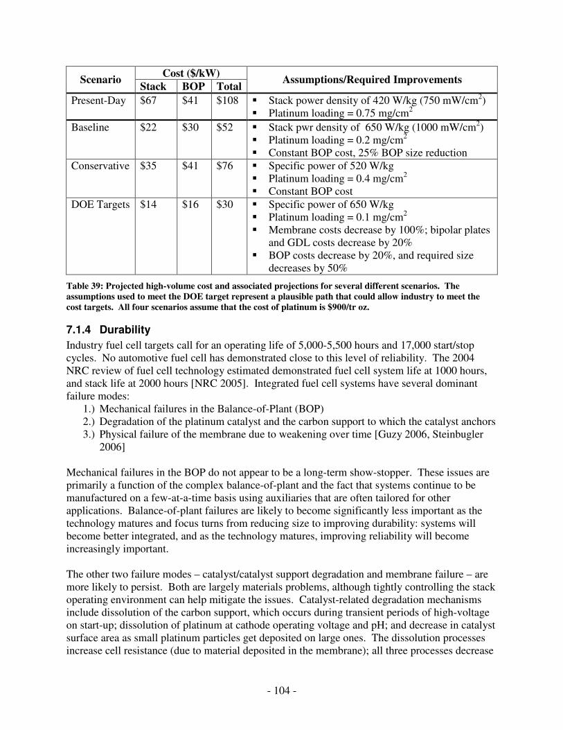
- 104 -

Cost ($/kW) Scenario

Stack BOP Total Assumptions/Required Improvements

Present-Day $67 $41 $108 Stack power density of 420 W/kg (750 mW/cm2) Platinum loading = 0.75 mg/cm2

Baseline $22 $30 $52 Stack pwr density of 650 W/kg (1000 mW/cm2) Platinum loading = 0.2 mg/cm2 Constant BOP cost, 25% BOP size reduction

Conservative

$35 $41 $76 Specific power of 520 W/kg Platinum loading = 0.4 mg/cm2 Constant BOP cost

DOE Targets $14 $16 $30 Specific power of 650 W/kg Platinum loading = 0.1 mg/cm2 Membrane costs decrease by 100%; bipolar plates

and GDL costs decrease by 20% BOP costs decrease by 20%, and required size

decreases by 50%

Table 39: Projected high-volume cost and associated projections for several different scenarios. The assumptions used to meet the DOE target represent a plausible path that could allow industry to meet the cost targets. All four scenarios assume that the cost of platinum is $900/tr oz.

7.1.4 Durability

Industry fuel cell targets call for an operating life of 5,000-5,500 hours and 17,000 start/stop cycles. No automotive fuel cell has demonstrated close to this level of reliability. The 2004 NRC review of fuel cell technology estimated demonstrated fuel cell system life at 1000 hours, and stack life at 2000 hours [NRC 2005]. Integrated fuel cell systems have several dominant failure modes:

1.) Mechanical failures in the Balance-of-Plant (BOP) 2.) Degradation of the platinum catalyst and the carbon support to which the catalyst anchors 3.) Physical failure of the membrane due to weakening over time [Guzy 2006, Steinbugler

2006] Mechanical failures in the BOP do not appear to be a long-term show-stopper. These issues are primarily a function of the complex balance-of-plant and the fact that systems continue to be manufactured on a few-at-a-time basis using auxiliaries that are often tailored for other applications. Balance-of-plant failures are likely to become significantly less important as the technology matures and focus turns from reducing size to improving durability: systems will become better integrated, and as the technology matures, improving reliability will become increasingly important. The other two failure modes – catalyst/catalyst support degradation and membrane failure – are more likely to persist. Both are largely materials problems, although tightly controlling the stack operating environment can help mitigate the issues. Catalyst-related degradation mechanisms include dissolution of the carbon support, which occurs during transient periods of high-voltage on start-up; dissolution of platinum at cathode operating voltage and pH; and decrease in catalyst surface area as small platinum particles get deposited on large ones. The dissolution processes increase cell resistance (due to material deposited in the membrane); all three processes decrease

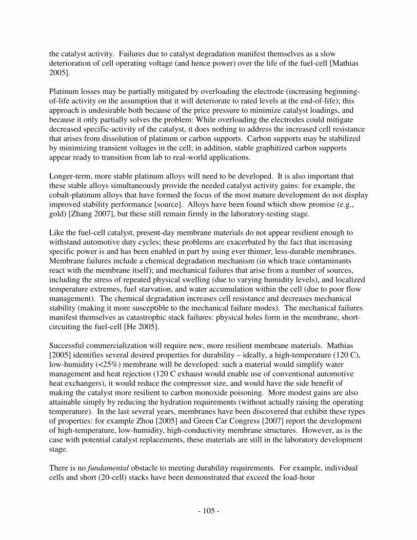
- 105 -

the catalyst activity. Failures due to catalyst degradation manifest themselves as a slow deterioration of cell operating voltage (and hence power) over the life of the fuel-cell [Mathias 2005]. Platinum losses may be partially mitigated by overloading the electrode (increasing beginning-of-life activity on the assumption that it will deteriorate to rated levels at the end-of-life); this approach is undesirable both because of the price pressure to minimize catalyst loadings, and because it only partially solves the problem: While overloading the electrodes could mitigate decreased specific-activity of the catalyst, it does nothing to address the increased cell resistance that arises from dissolution of platinum or carbon supports. Carbon supports may be stabilized by minimizing transient voltages in the cell; in addition, stable graphitized carbon supports appear ready to transition from lab to real-world applications. Longer-term, more stable platinum alloys will need to be developed. It is also important that these stable alloys simultaneously provide the needed catalyst activity gains: for example, the cobalt-platinum alloys that have formed the focus of the most mature development do not display improved stability performance [source]. Alloys have been found which show promise (e.g., gold) [Zhang 2007], but these still remain firmly in the laboratory-testing stage. Like the fuel-cell catalyst, present-day membrane materials do not appear resilient enough to withstand automotive duty cycles; these problems are exacerbated by the fact that increasing specific power is and has been enabled in part by using ever thinner, less-durable membranes. Membrane failures include a chemical degradation mechanism (in which trace contaminants react with the membrane itself); and mechanical failures that arise from a number of sources, including the stress of repeated physical swelling (due to varying humidity levels), and localized temperature extremes, fuel starvation, and water accumulation within the cell (due to poor flow management). The chemical degradation increases cell resistance and decreases mechanical stability (making it more susceptible to the mechanical failure modes). The mechanical failures manifest themselves as catastrophic stack failures: physical holes form in the membrane, short-circuiting the fuel-cell [He 2005]. Successful commercialization will require new, more resilient membrane materials. Mathias [2005] identifies several desired properties for durability – ideally, a high-temperature (120 C), low-humidity (<25%) membrane will be developed: such a material would simplify water management and heat rejection (120 C exhaust would enable use of conventional automotive heat exchangers), it would reduce the compressor size, and would have the side benefit of making the catalyst more resilient to carbon monoxide poisoning. More modest gains are also attainable simply by reducing the hydration requirements (without actually raising the operating temperature). In the last several years, membranes have been discovered that exhibit these types of properties: for example Zhou [2005] and Green Car Congress [2007] report the development of high-temperature, low-humidity, high-conductivity membrane structures. However, as is the case with potential catalyst replacements, these materials are still in the laboratory development stage. There is no fundamental obstacle to meeting durability requirements. For example, individual cells and short (20-cell) stacks have been demonstrated that exceed the load-hour

- 106 -

commercialization requirement and approach the start-stop requirement in a lab environment [Steinbugler 2006]. Similarly, membranes have lasted 20,000 cycles in controlled laboratory environments [Mathias 2005]. While this indicates that present-day membranes could do the job with more effective system management, it is inherently difficult to maintain humidity levels at high power. What is unclear is whether these tightly controlled laboratory tests may be successfully transferred to real-world load profiles and full-scale stacks (200-400 cells). Some industry analysts believe that continued development using the present approach to stack design – which entails driving size reductions by using thinner and thinner membranes – can meet the targets with incremental improvements in system control, membrane properties, and a transition to stable platinum alloys. Improvements to power density will also reduce the number of individual cells, decreasing the number of failure points. Others question whether the current approach can withstand the rigors of an automotive duty cycle without a dramatic breakthrough in membrane durability. The next 5 years should answer many of these questions: To date, industry has focused largely on weight and size reductions; in the next several years, this focus should shift more explicitly to improving durability.

7.2 Hydrogen Storage

A number of strategies for onboard hydrogen storage have been evaluated. These include high-pressure gaseous tanks, liquid-hydrogen tanks, sequestering hydrogen in metal- or chemical-hydrides or nano-tubes, and reforming hydrogen onboard from fossil-fuel primary inputs. The primary issues with the various direct-H2 storage systems are size, weight, and cost. Safety is also a concern with gaseous systems, but presumably could be handled if other pieces of the puzzle fall into place. The storage system would ideally be cost-competitive with a gasoline fuel-tank and fit within a similar form-factor (a typical mid-size sedan fuel-tank is 60-80L). There is a sense that onboard reforming of hydrogen does not make sense. While such an approach obviates the need for a new fueling infrastructure, it adds considerable complexity, cost, and size to the vehicle itself; it degrades the overall system efficiency; and impurities in the reformed fuel have a tendency to poison the fuel cell catalyst. For these reasons, industry has now largely focused efforts on developing direct H2 fuel cell systems. There is little reason to expect this trend to change.

Table 40: Characteristics of different 2004 hydrogen storage technologies. Source: NRC 2005

kWh/L kWh/kg Cost ($/kWh)

2015 Target 2.7 3.0 $2

Chemical Hydride 1.0 1.4 $8

Metal Hydride 0.6 0.8 $16

Liquid H2 1.2 1.7 $6

700 Bar 0.8 1.6 $18

350 Bar 0.5 1.9 $15

Table 40 summarizes the characteristics of present-day hydrogen storage systems, as well as the 2015 DOE targets. Nothing yet approaches these targets, and it is not at all clear that these goals are achievable in the near future: cost and performance must improve by a factor of 3 over the present-day state of the art. In order to meet the DOE targets, a breakthrough is needed. The volumetric efficiency of gaseous storage, the cost and complexity of metral hydrides, and the energy efficiency losses (as

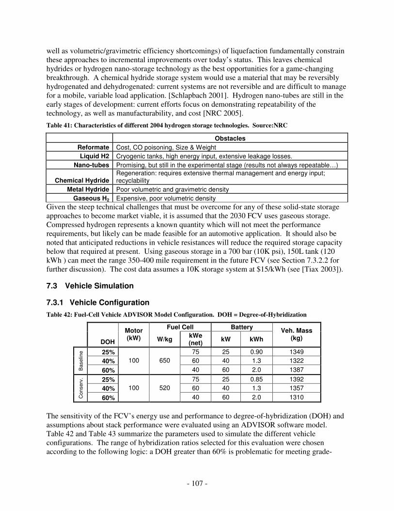
- 107 -

well as volumetric/gravimetric efficiency shortcomings) of liquefaction fundamentally constrain these approaches to incremental improvements over today’s status. This leaves chemical hydrides or hydrogen nano-storage technology as the best opportunities for a game-changing breakthrough. A chemical hydride storage system would use a material that may be reversibly hydrogenated and dehydrogenated: current systems are not reversible and are difficult to manage for a mobile, variable load application. [Schlapbach 2001]. Hydrogen nano-tubes are still in the early stages of development: current efforts focus on demonstrating repeatability of the technology, as well as manufacturability, and cost [NRC 2005].

Table 41: Characteristics of different 2004 hydrogen storage technologies. Source:NRC

Obstacles

Reformate Cost, CO poisoning, Size & Weight

Liquid H2 Cryogenic tanks, high energy input, extensive leakage losses.

Nano-tubes Promising, but still in the experimental stage (results not always repeatable…)

Chemical Hydride Regeneration: requires extensive thermal management and energy input; recyclability

Metal Hydride Poor volumetric and gravimetric density

Gaseous H2 Expensive, poor volumetric density

Given the steep technical challenges that must be overcome for any of these solid-state storage approaches to become market viable, it is assumed that the 2030 FCV uses gaseous storage. Compressed hydrogen represents a known quantity which will not meet the performance requirements, but likely can be made feasible for an automotive application. It should also be noted that anticipated reductions in vehicle resistances will reduce the required storage capacity below that required at present. Using gaseous storage in a 700 bar (10K psi), 150L tank (120 kWh ) can meet the range 350-400 mile requirement in the future FCV (see Section 7.3.2.2 for further discussion). The cost data assumes a 10K storage system at $15/kWh (see [Tiax 2003]).

7.3 Vehicle Simulation

7.3.1 Vehicle Configuration

Table 42: Fuel-Cell Vehicle ADVISOR Model Configuration. DOH = Degree-of-Hybridization

Fuel Cell Battery

DOH

Motor (kW) W/kg

kWe (net)

kW kWh

Veh. Mass (kg)

25% 75 25 0.90 1349

40% 60 40 1.3 1322

Baselin

e

60%

100 650

40 60 2.0 1387

25% 75 25 0.85 1392

40% 60 40 1.3 1357

Conserv

.

60%

100 520

40 60 2.0 1310

The sensitivity of the FCV’s energy use and performance to degree-of-hybridization (DOH) and assumptions about stack performance were evaluated using an ADVISOR software model. Table 42 and Table 43 summarize the parameters used to simulate the different vehicle configurations. The range of hybridization ratios selected for this evaluation were chosen according to the following logic: a DOH greater than 60% is problematic for meeting grade-

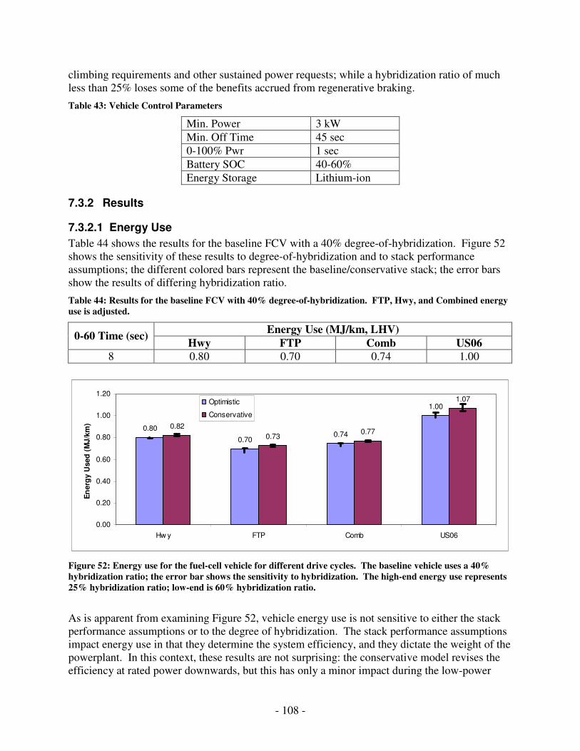
- 108 -

climbing requirements and other sustained power requests; while a hybridization ratio of much less than 25% loses some of the benefits accrued from regenerative braking.

Table 43: Vehicle Control Parameters

Min. Power 3 kW

Min. Off Time 45 sec

0-100% Pwr 1 sec

Battery SOC 40-60%

Energy Storage Lithium-ion

7.3.2 Results

7.3.2.1 Energy Use

Table 44 shows the results for the baseline FCV with a 40% degree-of-hybridization. Figure 52 shows the sensitivity of these results to degree-of-hybridization and to stack performance assumptions; the different colored bars represent the baseline/conservative stack; the error bars show the results of differing hybridization ratio.

Table 44: Results for the baseline FCV with 40% degree-of-hybridization. FTP, Hwy, and Combined energy use is adjusted.

Energy Use (MJ/km, LHV) 0-60 Time (sec)

Hwy FTP Comb US06 8 0.80 0.70 0.74 1.00

0.80

0.700.74

1.00

0.82

0.730.77

1.07

0.00

0.20

0.40

0.60

0.80

1.00

1.20

Hw y FTP Comb US06

En

erg

y U

sed

(M

J/k

m)

Optimistic

Conservative

Figure 52: Energy use for the fuel-cell vehicle for different drive cycles. The baseline vehicle uses a 40% hybridization ratio; the error bar shows the sensitivity to hybridization. The high-end energy use represents 25% hybridization ratio; low-end is 60% hybridization ratio.

As is apparent from examining Figure 52, vehicle energy use is not sensitive to either the stack performance assumptions or to the degree of hybridization. The stack performance assumptions impact energy use in that they determine the system efficiency, and they dictate the weight of the powerplant. In this context, these results are not surprising: the conservative model revises the efficiency at rated power downwards, but this has only a minor impact during the low-power

- 109 -

portions of the polarization curve – the efficiency at low power draw remains high even for the conservative model. While there is a minor weight impact in the conservative model due to the downward revision of the stack specific power, this is a difference of only a few tens of kilograms – not enough to dramatically change the picture. The performance benefits of hybridization accrue even at low hybridization ratios: these benefits primarily derive from regenerative braking (for which 25 kW is adequate under most normal driving) and from not operating the fuel-cell at very low-load, when efficiency is lowest (for which 3-5 kW is adequate). The primary performance benefit of higher hybridization ratios appears to derive from weight savings accrued from trading fuel-cell power for battery power. The real impact of varying hybridization and stack performance assumptions lies in their effect on system cost. The conservative stack assumes a lower specific power; as discussed in section 7.1.3, specific power should directly correlate with cost – so these assumptions have a minor impact on the energy use, but major impact on cost assessment. Similarly, varying the degree-of-hybridization is likely an economic calculus. Hybridizing essentially trades fuel-cell power for battery power, so this decision amounts to a question of whether a fuel-cell or battery are likely to be cheaper on a per-kW basis. In all likelihood, batteries will be cheaper than fuel-cells, which would dictate a shift towards more highly hybridized vehicles. At the same time, more highly hybridized vehicle could require a higher-energy battery, which could shift the economics back towards the fuel-cell. Accordingly, the 40% DOH vehicle is used as the baseline for future calculations.

7.3.2.2 Range

Table 45 shows the vehicle range that result from applying different hydrogen-storage pressure and tank size assumptions. As is apparent from the table, 700 bar storage with a 150L tank is necessary and sufficient to meet a 350-mile range requirement.

Table 45: Vehicle range for varying size and pressure hydrogen storage tanks. The low-end of the range represents the conservative, 25% DOH vehicle; the high-end corresponds to the baseline 60% DOH.

350 Bar 700 Bar

Tank (L) 90 150 90 150

Range (Mi) 156-168 260-280 234-252 390-420

7.3.2.3 Vehicle Price

Table 46 estimates the OEM cost of the fuel-cell vehicle on a component-by-component basis. This data assumes a 40% hybridization ratio. Both the baseline and conservative fuel-cell system cost estimate are included (the conservative calculation is in parentheses). Further details on sourcing and assumptions, as well as comparisons to other vehicles, are included in the results chapter.

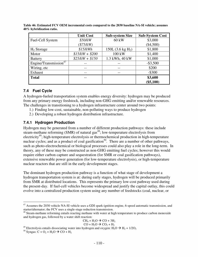
- 110 -

Table 46: Estimated FCV OEM incremental costs compared to the 2030 baseline NA-SI vehicle; assumes 40% hybridization ratio.

Unit Cost Sub-system Size Sub-System Cost Fuel-Cell System $50/kW

($75/kW) 60 kW $3,000

($4,500)

H2 Storage $15/kWh 150L (3.6 kg H2) $1,800

Motor $15/kW + $200 100 kW $1,400

Battery $25/kW + $150 1.3 kWh, 40 kW $1,000

Engine/Transmission47 -- -- -$3,500

Wiring, etc -- -- $200

Exhaust -- -- -$300

Total -- $3,600 ($5,100)

7.4 Fuel Cycle

A hydrogen-fueled transportation system enables energy diversity: hydrogen may be produced from any primary energy feedstock, including non-GHG emitting and/or renewable resources. The challenges in transitioning to a hydrogen infrastructure center around two points:

1.) Finding low-cost, sustainable, non-polluting ways to produce hydrogen 2.) Developing a robust hydrogen distribution infrastructure.

7.4.1 Hydrogen Production

Hydrogen may be generated from a number of different production pathways: these include steam-methane reforming (SMR) of natural gas48; low-temperature electrolysis from electricity49; high-temperature electrolysis or thermochemical production in high-temperature nuclear cycles; and as a product of coal gasification50. There are a number of other pathways, such as photo-electrochemical or biological processes could also play a role in the long-term. In theory, any of these may be constructed as non-GHG emitting fuel cycles; however this would require either carbon capture and sequestration (for SMR or coal gasification pathways), extensive renewable power generation (for low-temperature electrolysis), or high-temperature nuclear reactors that are still in the early development stages. The dominant hydrogen production pathway is a function of what stage of development a hydrogen transportation system is at: during early stages, hydrogen will be produced primarily from SMR at distributed locations. This represents the primary low-cost pathway used during the present-day. If fuel-cell vehicles become widespread and justify the capital outlay, this could evolve into a centralized production system using any number of feedstocks (coal, nuclear, or

47 Assumes the 2030 vehicle NA-SI vehicle uses a GDI spark-ignition engine, 6-speed automatic transmission, and starter/alternator; the FCV uses a single-stage reduction transmission. 48 Steam-methane reforming entails reacting methane with water at high temperature to produce carbon monoxide and hydrogen gas, followed by a water shift reaction:

CH4 + H2O CO + 3H2

CO + H2O CO2 + H2 49 Electrolysis entails dissociating water into hydrogen and oxygen: H2O H2 + 1/2O2 50 Syngas: C + O2 + H2O CO + H2

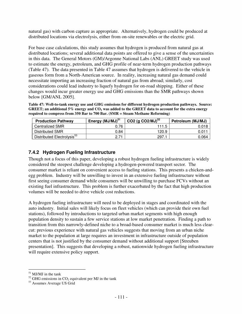
- 111 -

natural gas) with carbon capture as appropriate. Alternatively, hydrogen could be produced at distributed locations via electrolysis, either from on-site renewables or the electric grid. For base case calculations, this study assumes that hydrogen is produced from natural gas at distributed locations; several additional data points are offered to give a sense of the uncertainties in this data. The General Motors (GM)/Argonne National Labs (ANL) GREET study was used to estimate the energy, petroleum, and GHG profile of near-term hydrogen production pathways (Table 47). The data presented in Table 47 assumes that hydrogen is delivered to the vehicle in gaseous form from a North-American source. In reality, increasing natural gas demand could necessitate importing an increasing fraction of natural gas from abroad; similarly, cost considerations could lead industry to liquefy hydrogen for on-road shipping. Either of these changes would incur greater energy use and GHG emissions than the SMR pathways shown below [GM/ANL 2005].

Table 47: Well-to-tank energy use and GHG emissions for different hydrogen production pathways. Source: GREET; an additional 5% energy and CO2 was added to the GREET data to account for the extra energy required to compress from 350 Bar to 700 Bar. (SMR = Steam Methane Reforming)

Production Pathway Energy (MJ/MJ)51

CO2 (g CO2/MJ)52

Petroleum (MJ/MJ)

Centralized SMR 0.76 111.5 0.018

Distributed SMR 0.84 120.9 0.011

Distributed Electrolysis53

2.71 297.1 0.064

7.4.2 Hydrogen Fueling Infrastructure

Though not a focus of this paper, developing a robust hydrogen fueling infrastructure is widely considered the steepest challenge developing a hydrogen-powered transport sector. The consumer market is reliant on convenient access to fueling stations. This presents a chicken-and-egg problem. Industry will be unwilling to invest in an extensive fueling infrastructure without first seeing consumer demand while consumers will be unwilling to purchase FCVs without an existing fuel infrastructure. This problem is further exacerbated by the fact that high production volumes will be needed to drive vehicle cost reductions. A hydrogen fueling infrastructure will need to be deployed in stages and coordinated with the auto industry. Initial sales will likely focus on fleet vehicles (which can provide their own fuel stations), followed by introductions to targeted urban market segments with high enough population density to sustain a few service stations at low market penetration. Finding a path to transition from this narrowly-defined niche to a broad-based consumer market is much less clear-cut: previous experience with natural gas vehicles suggests that moving from an urban niche market to the population at large requires an investment in infrastructure outside of population centers that is not justified by the consumer demand without additional support [Streuben presentation]. This suggests that developing a robust, nationwide hydrogen fueling infrastructure will require extensive policy support.

51 MJ/MJ in the tank 52 GHG emissions in CO2 equivalent per MJ in the tank 53 Assumes Average US Grid

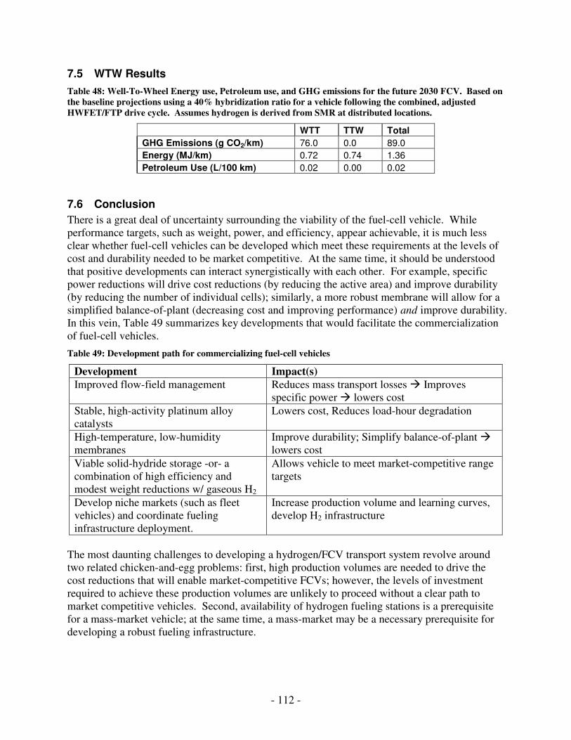
- 112 -

7.5 WTW Results

Table 48: Well-To-Wheel Energy use, Petroleum use, and GHG emissions for the future 2030 FCV. Based on the baseline projections using a 40% hybridization ratio for a vehicle following the combined, adjusted HWFET/FTP drive cycle. Assumes hydrogen is derived from SMR at distributed locations.

WTT TTW Total

GHG Emissions (g CO2/km) 76.0 0.0 89.0

Energy (MJ/km) 0.72 0.74 1.36

Petroleum Use (L/100 km) 0.02 0.00 0.02

7.6 Conclusion

There is a great deal of uncertainty surrounding the viability of the fuel-cell vehicle. While performance targets, such as weight, power, and efficiency, appear achievable, it is much less clear whether fuel-cell vehicles can be developed which meet these requirements at the levels of cost and durability needed to be market competitive. At the same time, it should be understood that positive developments can interact synergistically with each other. For example, specific power reductions will drive cost reductions (by reducing the active area) and improve durability (by reducing the number of individual cells); similarly, a more robust membrane will allow for a simplified balance-of-plant (decreasing cost and improving performance) and improve durability. In this vein, Table 49 summarizes key developments that would facilitate the commercialization of fuel-cell vehicles.

Table 49: Development path for commercializing fuel-cell vehicles

Development Impact(s) Improved flow-field management Reduces mass transport losses Improves

specific power lowers cost

Stable, high-activity platinum alloy catalysts

Lowers cost, Reduces load-hour degradation

High-temperature, low-humidity membranes

Improve durability; Simplify balance-of-plant lowers cost

Viable solid-hydride storage -or- a combination of high efficiency and modest weight reductions w/ gaseous H2

Allows vehicle to meet market-competitive range targets

Develop niche markets (such as fleet vehicles) and coordinate fueling infrastructure deployment.

Increase production volume and learning curves, develop H2 infrastructure

The most daunting challenges to developing a hydrogen/FCV transport system revolve around two related chicken-and-egg problems: first, high production volumes are needed to drive the cost reductions that will enable market-competitive FCVs; however, the levels of investment required to achieve these production volumes are unlikely to proceed without a clear path to market competitive vehicles. Second, availability of hydrogen fueling stations is a prerequisite for a mass-market vehicle; at the same time, a mass-market may be a necessary prerequisite for developing a robust fueling infrastructure.

- 113 -

These issues suggest that a hydrogen-fueled transport system would require significant policy incentives over a period of many years to initiate a transition. The key question then becomes whether the expense of transitioning to a hydrogen-fueled transportation system is justified by the likely marginal CO2 reduction benefits that will be realized from FCVs in the near- and mid-term. This question will be addressed in a more integrated fashion in Chapter 8.

- 114 -

8 Results

This chapter presents the integrated well-to-wheel results of the vehicle technology assessment. These results are first analyzed on a vehicle-by-vehicle basis to draw out the relative advantages and disadvantages of different technologies, then placed in the broader context of their potential to help meet GHG and petroleum reduction targets. Important Sensitivities: Before proceeding into detailed analysis, it is useful to identify several important factors that have a determinative outcome on the results: 1.) Implicit Constraints on Vehicle Configuration:

Vehicle performance and size remain unchanged from today’s levels. Vehicle resistances (weight, aerodynamics, rolling resistance) have decreased due to

evolutionary improvements. These two assumptions have a very strong impact on the results in an absolute sense, but should not have a significant impact on comparisons between vehicles. The implications of these implicit assumptions are briefly addressed in the Recommendations section. It should be noted that, aside from these constraints, the simulated tank-to-wheel energy use is surprisingly robust to variations in the study’s assumptions. In general, the components that constitute an electric powertrain (fuel-cell, lithium-ion battery, motor, etc) are highly efficient even today; varying these performance maps by a few percent does not dramatically impact the results. The most sensitive parameter in the tank-to-wheels results is the extent to which it is assumed that sophisticated vehicle integration can optimize the engine in a hybrid vehicle; a less optimistic assumption would downgrade the hybrid from a 43% improvement over the NA-SI to a 35% improvement. This change would also effect the plug-in hybrid, but to a lesser extent (due to its partial reliance on electricity).

2.) Fuel-Cycle Emissions In general, the fuel pathways which dominate are assumed to continue to do so: electricity is produced from a ‘business-as-usual’ average grid-mix; hydrogen is produced from natural gas using distributed generation; and petroleum is produced and refined using similar processes and sources that are currently used. However, fuel-cycle emissions depend greatly on the size of the market for a particular technology. This dictates whether the production processes are optimized to the technology in question, or whether other factors dictate. Fuel-cycle emissions also depend on the extent to which non-transportation sector energy and GHG emissions reductions are pursued. To address this uncertainty, data is presented which shows the fuel-cycle emissions for several different fuel production pathways (Figure 56); in addition, the prospects of reducing GHG emissions beyond the base case scenarios are discussed in qualitative terms.

3.) Cost Assumptions: In particular, long-term lithium-ion battery and fuel-cell cost projections are particularly speculative given that both have undergone rapid development in the last decade. In light of the uncertainty in these two dimensions, optimistic and conservative assumptions are noted in the individual chapters on electric vehicles and fuel cells (the two cases in which these uncertainties

- 115 -

are most prevalent). It does not appear that varying the cost assumptions within a reasonable envelope changes the qualitative sense of the conclusions.

Table 50: Energy use, petroleum use, and GHG emissions for all vehicle technologies over the combined, adjusted HWFET/FTP drive cycle.

2006

NA-SI 2030

NA-SI Turbo Diesel HEV

PHEV-10

PHEV-30

PHEV-60

BEV FCV

Fuel Cycle54:

Energy 0.24 0.24 0.24 0.21 0.24 0.47 0.85 1.16 2.30 0.84

GHG Emis. 21.2 21.2 21.2 19.0 21.2 40.6 81.3 119.3 213.6 121

Energy (MJ/km):

Well-to-Tank 0.65 0.40 0.36 0.20 0.23 0.37 0.57 0.71 1.24 0.62

Tnk-to-Wheel55 2.70 1.68 1.49 1.44 0.94 0.79 0.67 0.61 0.54 0.74

Well-to-Wheel 3.35 2.08 1.85 1.64 1.16 1.16 1.24 1.32 1.79 1.36

GHG Emis (gCO2/km):

Well-to-Tank 57.3 35.6 31.6 17.3 19.9 33.8 52.4 65.9 115.6 89.5

Tank-to-Wheel 194.4 120.6 107.2 109.8 67.4 50.5 33.8 23.9 -- --

Well-to-Wheel 251.7 156.2 138.8 127.1 87.3 84.3 86.2 89.8 115.6 89.5

Petrol (L/100 km, GE):

Tank-to-Wheel 8.85 5.49 4.88 4.73 3.08 2.30 1.54 1.09 -- --

54 Expressed in terms of g CO2 or MJ per MJ of fuel in the tank. For the plug-in hybrid vehicles, the well-to-tank and well-to-wheels data reflects a weighted average of electricity and gasoline. 55 Combusting gasoline is assumed to release 71.9 g CO2/MJ; combusting diesel is assumed to release 76.3 g CO2/MJ.

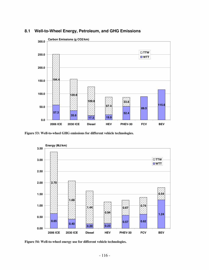
- 116 -

8.1 Well-to-Wheel Energy, Petroleum, and GHG Emissions

Carbon Emissions (g CO2/km)

57.335.6

17.3 19.9

52.4

89.5115.6

194.4

120.6

109.8

67.4

33.8

0.0

50.0

100.0

150.0

200.0

250.0

300.0

2006 ICE 2030 ICE Diesel HEV PHEV-30 FCV BEV

TTW

WTT

Figure 53: Well-to-wheel GHG emissions for different vehicle technologies.

Energy (MJ/km)

0.650.40

0.20 0.23

0.57 0.62

1.24

2.70

1.68

1.44

0.94

0.670.74

0.54

0.00

0.50

1.00

1.50

2.00

2.50

3.00

3.50

2006 ICE 2030 ICE Diesel HEV PHEV-30 FCV BEV

TTW

WTT

Figure 54: Well-to-wheel energy use for different vehicle technologies.

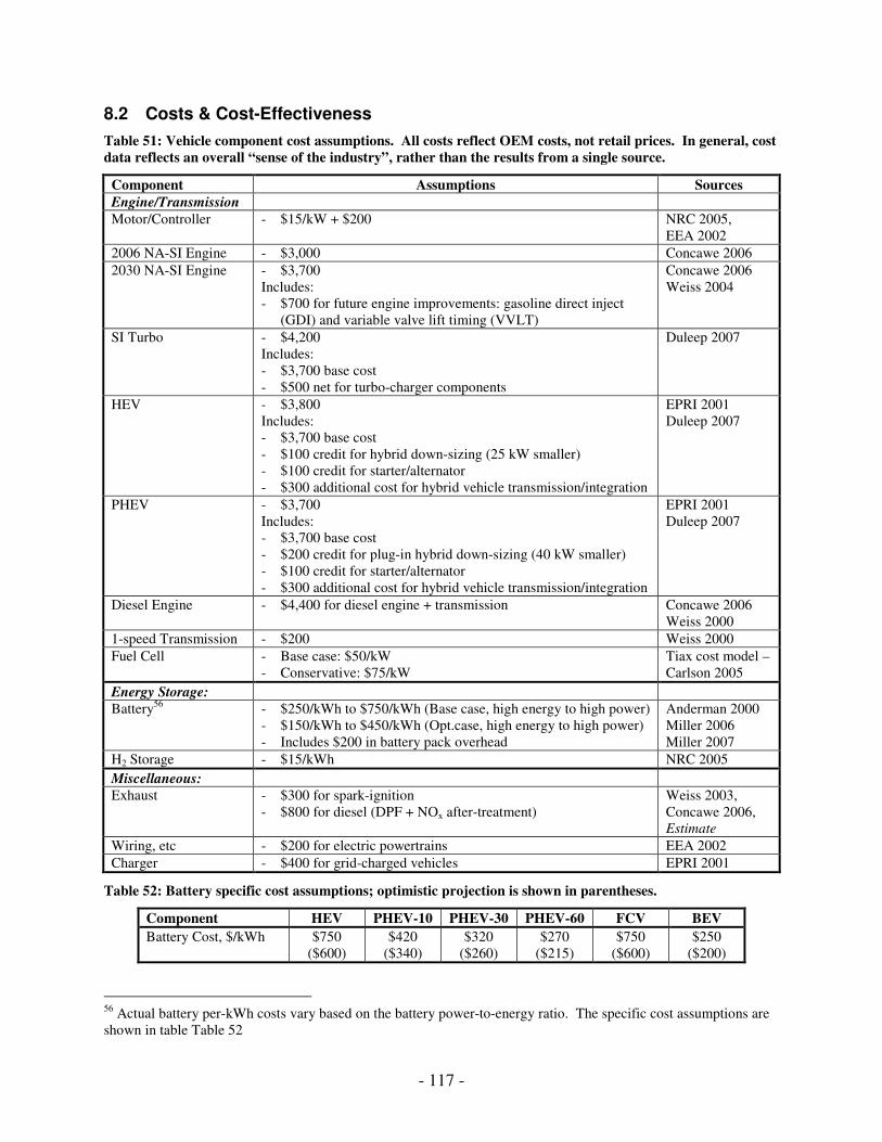
- 117 -

8.2 Costs & Cost-Effectiveness

Table 51: Vehicle component cost assumptions. All costs reflect OEM costs, not retail prices. In general, cost data reflects an overall “sense of the industry”, rather than the results from a single source.

Component Assumptions Sources Engine/Transmission

Motor/Controller - $15/kW + $200 NRC 2005, EEA 2002

2006 NA-SI Engine - $3,000 Concawe 2006

2030 NA-SI Engine - $3,700 Includes: - $700 for future engine improvements: gasoline direct inject

(GDI) and variable valve lift timing (VVLT)

Concawe 2006 Weiss 2004

SI Turbo - $4,200 Includes: - $3,700 base cost - $500 net for turbo-charger components

Duleep 2007

HEV - $3,800 Includes: - $3,700 base cost - $100 credit for hybrid down-sizing (25 kW smaller) - $100 credit for starter/alternator - $300 additional cost for hybrid vehicle transmission/integration

EPRI 2001 Duleep 2007

PHEV - $3,700 Includes: - $3,700 base cost - $200 credit for plug-in hybrid down-sizing (40 kW smaller) - $100 credit for starter/alternator - $300 additional cost for hybrid vehicle transmission/integration

EPRI 2001 Duleep 2007

Diesel Engine - $4,400 for diesel engine + transmission Concawe 2006 Weiss 2000

1-speed Transmission - $200 Weiss 2000

Fuel Cell - Base case: $50/kW - Conservative: $75/kW

Tiax cost model – Carlson 2005

Energy Storage:

Battery56

- $250/kWh to $750/kWh (Base case, high energy to high power) - $150/kWh to $450/kWh (Opt.case, high energy to high power) - Includes $200 in battery pack overhead

Anderman 2000 Miller 2006 Miller 2007

H2 Storage - $15/kWh NRC 2005

Miscellaneous:

Exhaust - $300 for spark-ignition - $800 for diesel (DPF + NOx after-treatment)

Weiss 2003, Concawe 2006, Estimate

Wiring, etc - $200 for electric powertrains EEA 2002

Charger - $400 for grid-charged vehicles EPRI 2001

Table 52: Battery specific cost assumptions; optimistic projection is shown in parentheses.

Component HEV PHEV-10 PHEV-30 PHEV-60 FCV BEV

Battery Cost, $/kWh $750 ($600)

$420 ($340)

$320 ($260)

$270 ($215)

$750 ($600)

$250 ($200)

56 Actual battery per-kWh costs vary based on the battery power-to-energy ratio. The specific cost assumptions are shown in table Table 52

- 118 -

Table 53: Estimated Incremental OEM Costs for vehicle technologies compared to the 2030 NA-SI. The impact of optimistic battery projections (based on $150/kWh for a high-energy battery) and conservative fuel-cell projections (based on $75/kW) are reflected in parentheses. Underlying assumptions are summarized in Table 51 and Table 52.

Component Turbo Diesel57 HEV PHEV-

10 PHEV-

30 PHEV-

60 FCV BEV

Drive Train:

Motor/Controller -- -- $600 $800 $800 $800 $1,400 $1,400

Engine/Transmission $500 $700 $200 $100 $100 $100 -$3,500 -$3,500

Fuel Cell -- -- -- -- -- -- $3,000 ($4,500)

--

Energy Storage:

Battery -- -- $900 ($750)

$1,500 ($1,200)

$2,800 ($2,200)

$4,600 ($3,700)

$1000 $12,000 ($8,600)

H2 Storage (150L) -- -- -- -- -- -- $1,800 --

Miscellaneous:

Exhaust $0 $500 $0 $0 $0 $0 -$300 -$300

Wiring, etc -- -- $200 $200 $200 $200 $200 $200

Charger -- -- -- $400 $400 $400 -- $400

Total $500 $1,200 $1,900 ($1,700)

$3,000 ($2,700)

$4,300 ($3,700)

$6,100 ($5,200)

$3,600 ($5,100)

$10,200 ($6,900)

Table 54: Costs-Effectiveness and fuel savings, relative to the 2030 NA-SI vehicle. Italics indicate optimistic

battery projection/conservative fuel-cell projection.

PHEV

Units NA-SI Turbo Diesel HEV 10 30 60

BEV FCV

Cost Effectiveness:

for Petroleum $/L --

$0.34 $0.66 $0.33 $0.29

$0.39 $0.35

$0.45 $0.40

$0.58 $0.49

$0.77 $0.52

$0.27 $0.39

for GHG $/ton --

$120 $172 $115 $103

$174 $157

$256 $226

$383 $326

$1,047 $708

$225 $319

Electric Range Mi 0 0 0 0 10 30 60 200 390

Fuel Costs58:

Gas Used Gal/Yr 330 300 290 190 150 100 70 -- --

Elec. Used kWh/Yr -- -- -- -- 660 1,470 2,040 4,000 --

H2 Used kg/Yr -- -- -- -- -- -- -- -- 150

Gas Cost $/Yr $1000 $900 $860 $560 $420 $280 $200 $0 $0

Elec Cost $/Yr -- -- -- -- $30 $75 $100 $200 $0

H2 Cost $/Yr -- -- -- -- -- -- -- -- $525

Tot. Fuel Cost $/Yr $1000 $900 $860 $560 $450 $355 $300 $200 $525

Yearly Savings $/Yr -- $100 $140 $440 $550 $645 $700 $800 $475

57 The diesel engine cost increment is relative to a 2030 NA-SI engine, which is expected to be more expensive due to technological improvements. 58 Assumptions: gas costs $3.00/gallon gasoline equivalent; electricity costs $0.05/kWh; hydrogen costs $3.50/kg [NRC 2004]; 15,000 miles per year (for yearly savings), 150,000 mile lifetime (for total cost-effectiveness).

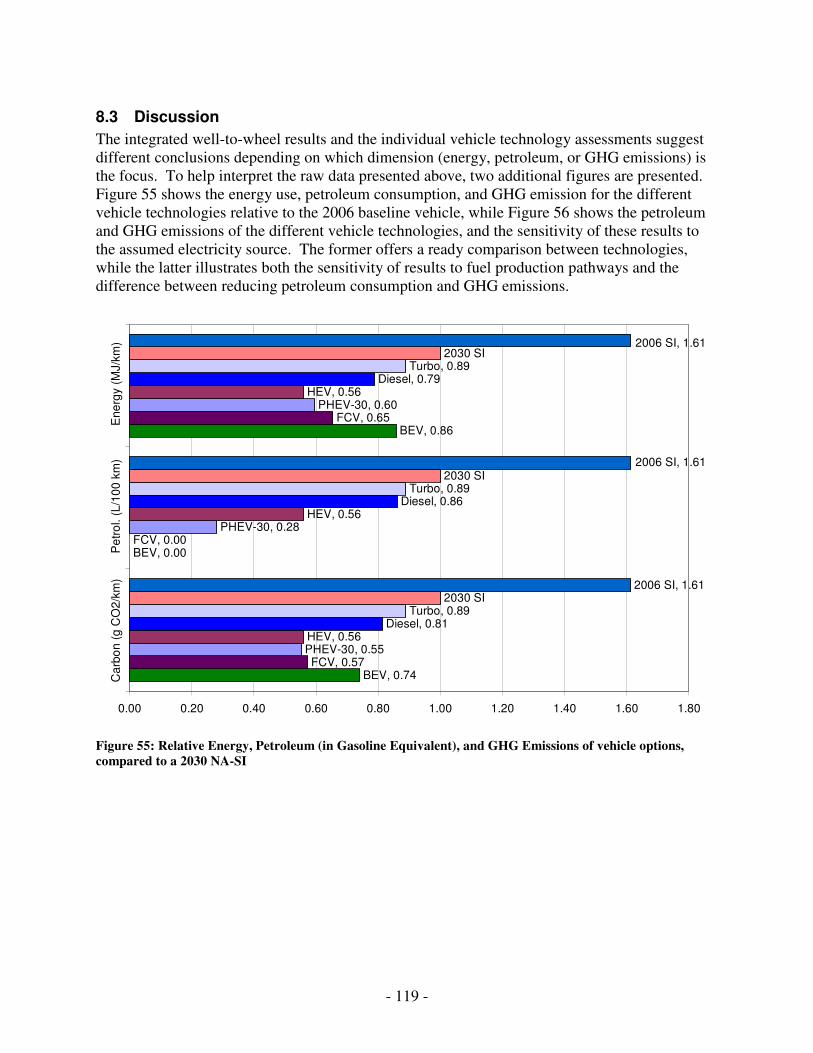
- 119 -

8.3 Discussion

The integrated well-to-wheel results and the individual vehicle technology assessments suggest different conclusions depending on which dimension (energy, petroleum, or GHG emissions) is the focus. To help interpret the raw data presented above, two additional figures are presented. Figure 55 shows the energy use, petroleum consumption, and GHG emission for the different vehicle technologies relative to the 2006 baseline vehicle, while Figure 56 shows the petroleum and GHG emissions of the different vehicle technologies, and the sensitivity of these results to the assumed electricity source. The former offers a ready comparison between technologies, while the latter illustrates both the sensitivity of results to fuel production pathways and the difference between reducing petroleum consumption and GHG emissions.

BEV, 0.74

BEV, 0.00

BEV, 0.86

FCV, 0.57

FCV, 0.00

FCV, 0.65

PHEV-30, 0.55

PHEV-30, 0.28

PHEV-30, 0.60

HEV, 0.56

HEV, 0.56

HEV, 0.56

Diesel, 0.81

Diesel, 0.86

Diesel, 0.79

Turbo, 0.89

Turbo, 0.89

Turbo, 0.89

2030 SI

2030 SI

2030 SI

2006 SI, 1.61

2006 SI, 1.61

2006 SI, 1.61

0.00 0.20 0.40 0.60 0.80 1.00 1.20 1.40 1.60 1.80

Ca

rbo

n (

g C

O2

/km

) P

etr

ol.

(L/1

00

km

) E

ne

rgy (

MJ/k

m)

Figure 55: Relative Energy, Petroleum (in Gasoline Equivalent), and GHG Emissions of vehicle options, compared to a 2030 NA-SI

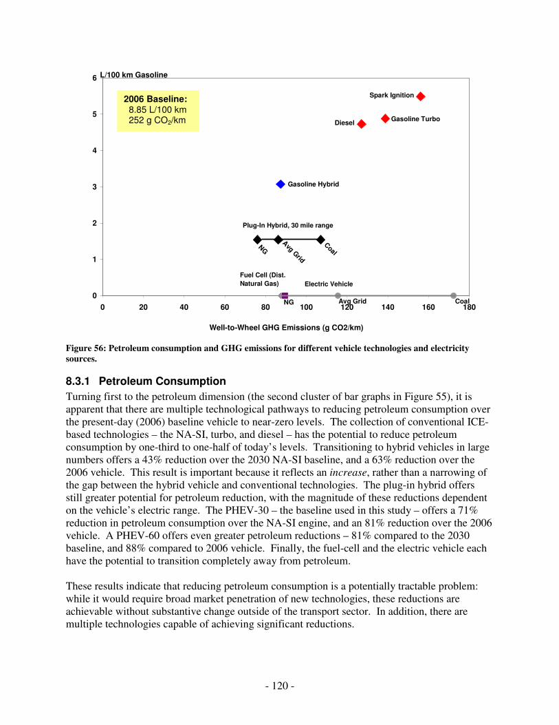
- 120 -

Spark Ignition

DieselGasoline Turbo

Gasoline Hybrid

Coal

NG

Avg G

rid

CoalNG Avg Grid0

1

2

3

4

5

6

0 20 40 60 80 100 120 140 160 180

Well-to-Wheel GHG Emissions (g CO2/km)

L/100 km Gasoline

Plug-In Hybrid, 30 mile range

Fuel Cell (Dist.

Natural Gas) Electric Vehicle

Figure 56: Petroleum consumption and GHG emissions for different vehicle technologies and electricity sources.

8.3.1 Petroleum Consumption

Turning first to the petroleum dimension (the second cluster of bar graphs in Figure 55), it is apparent that there are multiple technological pathways to reducing petroleum consumption over the present-day (2006) baseline vehicle to near-zero levels. The collection of conventional ICE-based technologies – the NA-SI, turbo, and diesel – has the potential to reduce petroleum consumption by one-third to one-half of today’s levels. Transitioning to hybrid vehicles in large numbers offers a 43% reduction over the 2030 NA-SI baseline, and a 63% reduction over the 2006 vehicle. This result is important because it reflects an increase, rather than a narrowing of the gap between the hybrid vehicle and conventional technologies. The plug-in hybrid offers still greater potential for petroleum reduction, with the magnitude of these reductions dependent on the vehicle’s electric range. The PHEV-30 – the baseline used in this study – offers a 71% reduction in petroleum consumption over the NA-SI engine, and an 81% reduction over the 2006 vehicle. A PHEV-60 offers even greater petroleum reductions – 81% compared to the 2030 baseline, and 88% compared to 2006 vehicle. Finally, the fuel-cell and the electric vehicle each have the potential to transition completely away from petroleum. These results indicate that reducing petroleum consumption is a potentially tractable problem: while it would require broad market penetration of new technologies, these reductions are achievable without substantive change outside of the transport sector. In addition, there are multiple technologies capable of achieving significant reductions.

2006 Baseline: 8.85 L/100 km 252 g CO2/km

- 121 -

8.3.2 GHG Emissions and Energy Use

Achieving the same magnitude reduction in the light-duty fleet’s primary energy use and GHG-emissions presents a much greater challenge. While the base case projections for of the advanced technologies show a dramatic improvement over the 2030 baseline (a 40-45% reduction), these projections cluster around similar levels. Going beyond this level of improvement requires changes that go beyond a transition to a new powertrain. In the case of primary energy consumption, improvements (on a per-vehicle basis) are largely restricted to reducing vehicle resistances; this is because the well-to-tank fuel cycle for the alternative fuels under evaluation (hydrogen and electricity production), are quite energy intensive and difficult to change. Additional per-vehicle reductions in greenhouse-gas emissions may be achieved either by additional reductions in vehicle resistances or by reducing GHG emissions in the alternative fuel cycles. The relative difficulty of achieving these additional carbon reductions varies greatly depending on the fuel and vehicle technology.

Table 55: Fuel-cycle GHG-reduction opportunities beyond the base-case projections

NA-SI, Diesel, HEV

- Bio-fuels

Plug-In - Bio-fuels - Reduced GHG emissions from electricity generation - Adjust electric range to maximize the CO2 benefit

FCV - Non-emitting H2 production pathways

BEV - Reduced GHG emissions from electricity generation

Bio-Fuels: For the vehicles that rely exclusively on petroleum – the hybrid, the diesel, and the spark-ignition – the only viable pathway to reduce the carbon content of the fuel is through the increased use of bio-fuels. The widespread use of bio-fuels faces two important challenges: 1.) Producing these fuels via non-GHG emitting pathways; and 2.) Implementing bio-fuel production at scale. Answering these challenges will likely require a transition away from the corn-based ethanol (using a starch conversion process) that currently dominates US ethanol production to a production pathway that uses ligno-cellulosic conversion technology. While the cellulosic technology is currently more expensive, it appears to be economically feasible with continued development. Even with the successful implementation of ligno-cellulosic processes, bio-fuels will likely be constrained by land and water-use restrictions to 100-200 billion liters of gasoline-equivalent (150-300 billion liters of ethanol) production per year in the long run [Groode]. As point of reference, current US light-duty petroleum demand is 570 billion liters, and is expected to grow to 820 billion liters by 2030; current ethanol production is about 15 billion liters per year [EIA]. Electric Grid: The emissions from grid-sourced energy used to power plug-in hybrid or battery-electric vehicles may be reduced by lowering the emissions rate of the electric sector. This emissions rate varies substantially based on the fuel source and prime mover. Neither the plug-in hybrid nor the BEV

- 122 -

offer GHG-reduction benefits when compared to the conventional hybrid under the business-as-usual average grid mix assumption, and the GHG profile is demonstrably worse if the vehicles are charged primarily from coal-fired power plants without carbon capture. On the other hand, as the charging regime moves to less-polluting sources, such as natural gas, renewables, nuclear, or fossil plants with carbon capture and sequestration, and higher efficiency prime-movers, such as combined-cycle plants, the GHG reduction benefits of grid-sourced energy become significantly greater than that obtained from the hybrid vehicle using petroleum from conventional sources. This sensitivity is illustrated in Figure 56, which shows the impact of varying the fraction of generation between 100% coal (the far right data point for both the PHEV and BEV), and the fraction that comes from natural gas (the far left data point). Increasing the fraction of renewable generation or generation efficiency of the grid would shift the GHG emissions still lower. How likely is such a shift toward cleaner power generation? The slow rate of fleet turnover in the power sector (a typical plant may be licensed for 40 years of operation) would suggest a long lead time for this type of systemic change. In addition, the EIA base case projection shows that supply shortfalls due to tightening natural gas supplies and decommissioning of nuclear plants over the next 30 years will be met primarily by new coal generation. At the same time, the electricity sector is well-positioned to deploy GHG emission reductions as part of a continuous, incremental process – particularly if there are appropriate price signals. There are many pathways to reduce GHG emissions in the electric sector, and perhaps more importantly, there is increasing discussion in policy circles at both the state and federal level focused on deploying these options at scale. At present, 15 states are scheduled to implement a CO2 trading system for the electric sector in the next several years, and 23 states have a renewable portfolio standard [Pew 2007]. Time will tell how successful these state-level programs will be, but it seems increasingly likely that the electric sector will be subjected to some type of federal CO2 regulation in the next several years. These factors suggest that additional GHG reductions beyond the EIA base case projection from grid-charged vehicles are comparatively likely. Hydrogen: For the hydrogen fuel-cell, additional GHG reductions may be achieved by developing low-emitting hydrogen production pathways. While there are a number of such options, it will be very difficult to do so economically in the foreseeable future: unlike electric generation, there does not appear to be a clear continuous path for reducing the GHG footprint of hydrogen production. Centralized production of hydrogen requires extensive capital investment in plants and pipelines that are difficult to implement incrementally and difficult to justify without a large market already in place. In addition, the technology to implement such centralized non-emitting pathways – such as high-temperature electrolysis in nuclear reactors, or fossil generation with carbon-capture – does not yet exist. Low-GHG emitting distributed hydrogen production paths include electrolysis powered either by a much cleaner electric grid or by distributed renewables. However, electrolysis from the electric grid is prohibitively energy intensive and expensive: as a point of reference, the electric grid must reduce its emissions rate to 38% of the projected level to achieve lower GHG emissions than steam reforming, requires 3 times more energy, and is estimated to cost about twice as much as a distributed natural gas pathway [NRC]. Using distributed renewables to produce hydrogen presents the most viable path near-term path for reducing the fuel-cycle GHG emissions: while the process remains energy intensive and is likely

- 123 -

to be expensive, using hydrogen production as an energy storage medium offers an opportunity to take advantage of wind and solar resources that are difficult to integrate into the electric grid because they are not dispatchable.

Table 56: Summary of the outlook for reducing GHG emissions through additional use of low carbon fuels. The two right-most columns offer a qualitative judgment of 1.) How difficult it is to implement change at large scale; and 2.) The technical risk involved in developing clean production pathways. Lighter shading

implies a lesser challenge.

Difficulty Fuel Important Considerations

Scale Tech Risk

Bio-fuels - Scale may be constrained by land-area requirements. - Requires development of low-cost cellulosic process

Hydrogen

- Electrolysis from renewable resources is expensive and energy intensive - Centralized generation requires distribution infrastructure, technological development, and/or broad systemic change - Difficult to implement incrementally

Electricity

- Requires systemic change in the electric sector (perhaps monetization of CO2) - CO2 reductions in the electric sector are comparatively cheap - Ability to leverage cap-and-trade policies and renewable mandates in the electric sector to clean up the transport sector

The key finding suggested by this analysis is that broad deployment of low-emissions vehicles does not guarantee low lifecycle emissions. In reality, the GHG benefit of vehicle technologies and alternative fuels is very sensitive to the fuel production process. Table 56 offers a qualitative summary of the key obstacles and assessment of the relative difficulty in pursuing these additional reductions beyond the base case projection: improvements in the electric sector appear comparatively easy to come by, and are likely to happen as part of any comprehensive GHG reduction plan; bio-fuels appear feasible, but may be constrained in scale; and hydrogen appears surprisingly difficult to produce from non-emitting pathways.

8.3.3 Vehicle technology outlook:

Table 57: Technological challenges to deployment at scale for advanced electric powertrains. Lighter colored boxes indicate lower technical risk.

Energy Storage Power Plant Infrastructure HEV - Battery cost

- Demonstrate durability - Engine Optimization N/A

Plug-In - Duty cycle - Battery cost

- Dual Mode Integration - Induce off-peak recharge - Availability of outlets

FCV - >300 mile range - Reduce cost

- Durable membrane - Stable, active Pt alloy - Balance-of-plant cost

- H2 fueling infrastructure - H2 production at scale.

BEV - 2X reduction in Li-ion battery costs - Range/cost tradeoff

- N/A - Rapid recharge stations - Special residential outlets - Grid capacity?

- 124 -

Taken as a group, the electric powertrains all offer significant improvements over the conventional options in terms of both petroleum consumption and GHG emissions. However, these improvements come at different cost, with different barriers to entering the market in large numbers, and with different constraints on their potential for continued improvement. Table 57 summarizes the important technological challenges to deploying the different vehicle technologies. The vehicles options are listed loosely in order of the scope of the challenge needed to implement at scale. HEV: The results of the technical evaluation offer a comparatively optimistic assessment of the hybrid-electric vehicle. As a relatively new technology, there is reason to believe that continued improvement relative to the conventional technologies is likely. These improvements are projected to arise largely from improved vehicle integration, which allows for tightly optimized control of the engine operating points. In addition, due in part to scale economies and in part to significant reductions in the cost of high-power batteries, the incremental costs of the hybrid are expected to decrease relative to conventional technologies. While questions have been raised about the robustness of the hybrid vehicle’s fuel consumption benefits to both high accessory loads and to aggressive drive cycles, are likely to become less important with continued technological development and seem to have been overstated in the first place. As a technology that has already enjoyed market success and has already penetrated the market in small numbers, the hybrid vehicle faces the least technical risk and the greatest leverage for reducing petroleum and GHG emissions in the near-term amongst the technologies under evaluation. The primary drawback of the hybrid is that, because it continues to derive all of its power from gasoline, it is fundamentally constrained in terms of both petroleum and GHG emission reductions by the extent to which low-carbon bio-fuels are deployed. PHEV: The plug-in hybrid offers a striking opportunity to reduce petroleum consumption to a level half of that offered by the hybrid vehicle. In addition, while the plug-in hybrid’s business-as-usual GHG emissions do not project a significant benefit, they offer a continuous path for incremental improvement through decreased carbonization of the power sector – an opportunity that does not exist for the hybrid vehicle. Moreover, because the PHEV can greatly reduce the fleet petroleum requirement, it can mitigate the scale constraint of biofuels. Whereas bio-fuels might be able to meet only 20% of the transportation energy requirement in an NA-SI dominated fleet, it could conceivably meet the entire petroleum requirement in a plug-in hybrid-dominated fleet. In essence, the plug-in hybrid creates a flexible pathway to GHG reductions: transportation-sector CO2 reductions may be pursued by either reducing the emissions rate of the electric grid or by increasing the fraction of biofuels. Varying the vehicle’s electric range offers an additional element of flexibility for increasing the projected GHG benefit: while the base case projection for GHG emissions does not change substantially for PHEVs with different range, the relative contribution from electricity and petroleum varies a great deal. Should the emissions rate of the electric grid improve significantly, a shift to higher range vehicles could be justified.

- 125 -

At the same time, the PHEV is a less cost-effective way to reduce petroleum and greenhouse gas emissions than the hybrid (particularly in the near-term); and, due to its higher upfront cost, it will have a harder time penetrating the market (see Table 54). The plug-in hybrid also faces greater technical and infrastructure risk than the HEV: while the hybrid has already enjoyed market success, the plug-in hybrid still requires significant improvements in battery technology to meet the rigors of an automotive duty cycle. And while the infrastructure for supporting hybrid vehicles is already mature, deploying the plug-in hybrid at scale will require regulation to ensure that off-peak generation capacity is used; depending on geography, it could also require capacity expansion. While the infrastructure issues represent a relatively low barrier to deployment, the technical challenges will delay the time-to-market for the plug-in hybrid. Taken together, the long time to market penetration and the lower cost-effectiveness of the plug-in hybrid suggest that the HEV offers a higher leverage, lower-cost path to reducing petroleum and GHG emissions in the near-term. However, given the upper bound on the HEV’s effectiveness, the plug-in hybrid offers a mid- to long-term path to continued reductions. The plug-in hybrid looks particularly promising over the mid- and long-term scenarios when contrasted with the technical risk, cost, range limitations, and infrastructure challenges associated with the fuel-cell and the electric vehicle – particularly should the technological development of the fuel-cell stall. Due to its lower weight, it also uses less energy and produces fewer GHG emissions on a well-to-wheel basis than the BEV59. And while at first blush it might appear that the PHEV suffers from a ceiling on its GHG reduction benefit due to its continued reliance on petroleum, the magnitude of petroleum reduction offered by even the 30-mile electric range (5X less than the present-day baseline) is such that this demand could conceivably be met by biofuels. Fuel-Cell: The fuel-cell vehicle has the ultimate potential to dramatically decrease GHG emissions and reliance on petroleum, but it requires the deployment of a new fueling infrastructure and must still overcome a number of daunting technological obstacles. These long-term challenges revolve around developing a fuel-cell that can withstand the rigors of an automotive duty-cycle over the life of the vehicle, reducing system cost, and developing low-cost hydrogen storage that allows for more than 300 miles range. While these challenges are significant, it is important to recognize that the fuel-cell is a new technology that has improved by leaps and bounds in the last decade; the key question is how long this rapid development can continue. It is not clear how to develop hydrogen production paths that allow the fuel-cell vehicle to fully realize its potential for near-zero GHG emissions and fossil-fuel consumption. Natural gas feedstocks are likely to offer the cheapest and least-polluting hydrogen production pathway for decades. However, given that North American natural gas supplies are already stretched thin, this begs the question of whether a hydrogen-fueled transportation system will trade reliance on one imported fossil fuel (petroleum) for a different one (natural gas). The other alternative to reformed natural gas is a shift to domestic production pathways; as a whole, these tend to be

59 At first blush, the large difference between the BEV and PHEV energy use is somewhat surprising. This difference is due to the BEV’s higher weight. Because there are fewer other sources of loss, weight differences in an electric drivetrain have a greater impact than similar weight differences in a conventional vehicle.

- 126 -

some combination of more energy intensive, higher emitting, difficult to implement at scale, or expensive. In addition, while not a major focus of this study, the fuel-cell requires significantly more energy to manufacture than the hybrid, plug-in hybrid, or NA-SI vehicles; this margin may decrease in the future as technology matures (see Section 2.7 for further discussion). This is an important consideration, particularly considering how close the base case well-to-wheel GHG projections are between different advanced vehicle technologies. Even with successful and rapid development of the technology, the scope of the challenge associated with deploying a brand-new technology and fueling infrastructure are such that it will take a long time for the fuel-cell to penetrate the market in large numbers. Moreover, it may be very difficult to further reduce the FCV’s GHG emissions below that of the base-case projections. BEV: Over the time horizon in question, the plug-in hybrid vehicle appears to be a more viable technology than the battery-electric vehicle for a mass-market consumer. It is assumed that a BEV with a 200-mile electric range is needed to approach the level of utility expected by the consumer and offered by other technologies. Even with this limited driving range, the electric vehicle is likely to come at an OEM cost increment of over $10,000 – far greater than that projected for any of the other vehicle technologies. Even with optimistic battery cost projections, the incremental cost of the BEV sits at the high end of the projected technology costs ($7,000, and these optimistic cost projections would presumably carry over to the other technologies). In addition, due to the weight of the battery pack, the BEV is projected to offer lower GHG and energy reductions than the FCV, HEV, or PHEV. While the BEV may be recharged from home, this: 1.) Does not address the range limitation on long car trips, and 2.) Would likely require the installation of dedicated high-power (220V, 50A) charging outlets for residential recharge. As such, a transportation system based around the electric vehicle would require the deployment of an electrical refueling infrastructure to address the range limitations – a task that is less daunting than deploying a hydrogen infrastructure, but is still a significant challenge. While there is already an electricity distribution network in place (i.e., the electric grid), there are few electric fueling stations. These barriers lie in particularly stark contrast to the plug-in hybrid. The PHEV offers much of the petroleum reduction benefit of the BEV and greater near-term CO2 and energy benefits, at much lower cost. In addition, the PHEV requires minimal additional infrastructure and is not range-limited. In the future, should battery technology and the emissions from the electric grid progress to the point that the BEV makes sense on a societal level, a transition from a plug-in hybrid-dominated fleet to a BEV-dominated fleet would be comparatively smooth: consumers would have already accepted the idea of grid-charged vehicles and there would likely be some limited recharge infrastructure in place. This analysis is not meant to imply the BEV cannot enter and be successful in the market as a niche vehicle (for example, as a commuter car, or as a “green” sports or luxury car), but rather that the technical challenges are too steep for the BEV to succeed in the mass market in the next several decades. Over a longer time horizon, a combination of improved battery technology and resource constraints may eventually necessitate an all-electric transportation system.

- 127 -

8.3.4 Fleet Implications

To this point, this study has quantified the potential of advanced electric powertrains to reduce petroleum consumption and greenhouse gas emissions on a per-vehicle basis. The challenge now is to place these results in the broader context of the US light-duty fleet. To gain this broader context, the GHG emissions and petroleum consumption of different vehicle technology penetration scenarios are compared to mid-century targets. In the case of GHG emissions, the target is based on a 550 ppm atmospheric CO2 stabilization target such as that identified in Kuuskraa [2006]; for petroleum consumption, the target is based on a goal of zero petroleum imports. Both targets use the year 2050 as a reference date. Stabilizing GHG emissions at 550 ppm requires that the total US CO2 emissions drop to 4400 million Mtons of CO2-equivalent by 2050, a level that is 40% of the business-as-usual projections (about 12,000 mMTons)60. In addition, achieving this stabilization level will require continued GHG reductions into the second half of the century. If it is assumed that the GHG emissions reduction required from the light-duty transport sector is proportional to its contribution to overall GHG emissions, then light-duty transport must also reduce its emissions by a factor of 2.7 by 2050 and be positioned to continue these reductions.

Annual Petroleum Consumption (Billion L)

0

200

400

600

800

1000

1200

2005 2010 2015 2020 2025 2030 2035 2040 2045 2050

Imports

Domestic

660 Billion Liters

Figure 57: Projected domestic and imported petroleum consumption, 2005-2050 [EIA 2006].

60 There is a wide range of numbers quoted in the literature regarding an appropriate value for the reference case (“business as usual”) GHG emissions; for the purposes of this discussion, the important point is that about a 60% reduction is required.

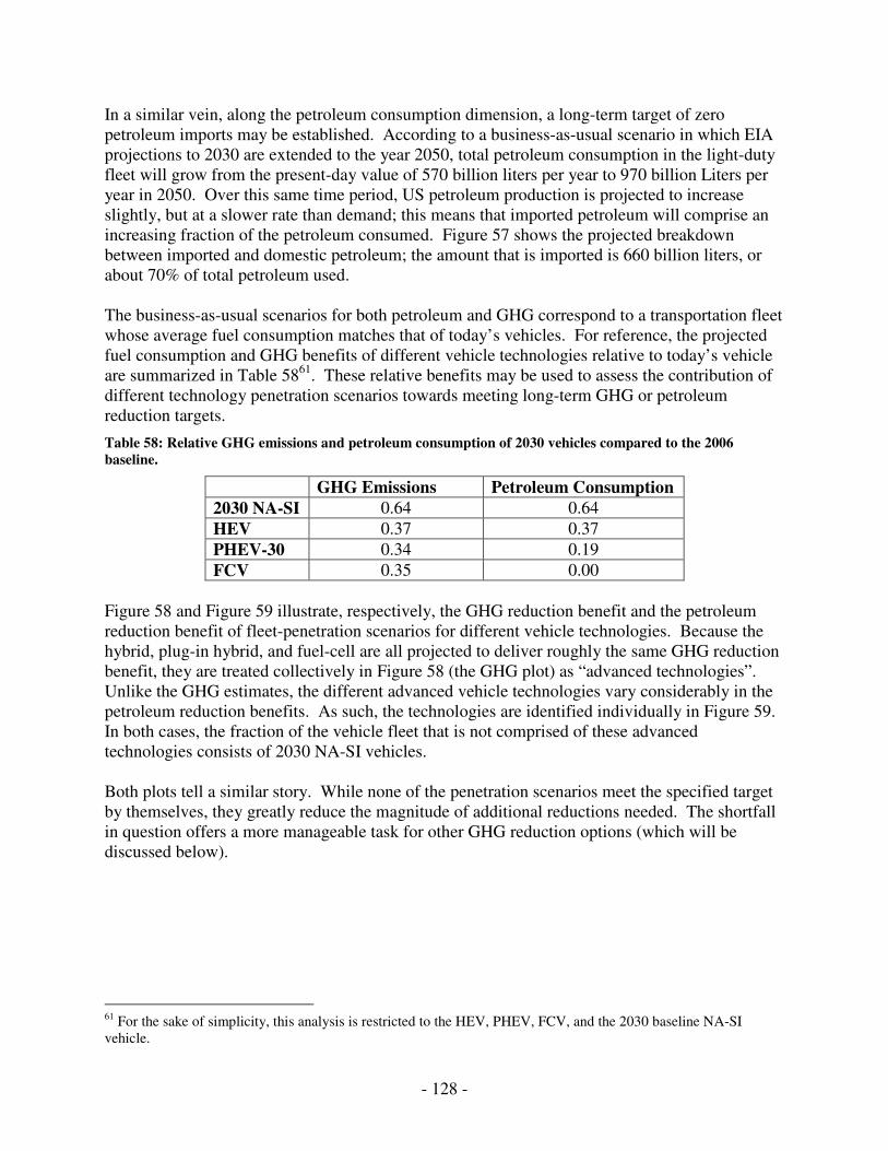
- 128 -

In a similar vein, along the petroleum consumption dimension, a long-term target of zero petroleum imports may be established. According to a business-as-usual scenario in which EIA projections to 2030 are extended to the year 2050, total petroleum consumption in the light-duty fleet will grow from the present-day value of 570 billion liters per year to 970 billion Liters per year in 2050. Over this same time period, US petroleum production is projected to increase slightly, but at a slower rate than demand; this means that imported petroleum will comprise an increasing fraction of the petroleum consumed. Figure 57 shows the projected breakdown between imported and domestic petroleum; the amount that is imported is 660 billion liters, or about 70% of total petroleum used. The business-as-usual scenarios for both petroleum and GHG correspond to a transportation fleet whose average fuel consumption matches that of today’s vehicles. For reference, the projected fuel consumption and GHG benefits of different vehicle technologies relative to today’s vehicle are summarized in Table 5861. These relative benefits may be used to assess the contribution of different technology penetration scenarios towards meeting long-term GHG or petroleum reduction targets.

Table 58: Relative GHG emissions and petroleum consumption of 2030 vehicles compared to the 2006 baseline.

GHG Emissions Petroleum Consumption

2030 NA-SI 0.64 0.64

HEV 0.37 0.37

PHEV-30 0.34 0.19

FCV 0.35 0.00

Figure 58 and Figure 59 illustrate, respectively, the GHG reduction benefit and the petroleum reduction benefit of fleet-penetration scenarios for different vehicle technologies. Because the hybrid, plug-in hybrid, and fuel-cell are all projected to deliver roughly the same GHG reduction benefit, they are treated collectively in Figure 58 (the GHG plot) as “advanced technologies”. Unlike the GHG estimates, the different advanced vehicle technologies vary considerably in the petroleum reduction benefits. As such, the technologies are identified individually in Figure 59. In both cases, the fraction of the vehicle fleet that is not comprised of these advanced technologies consists of 2030 NA-SI vehicles. Both plots tell a similar story. While none of the penetration scenarios meet the specified target by themselves, they greatly reduce the magnitude of additional reductions needed. The shortfall in question offers a more manageable task for other GHG reduction options (which will be discussed below).

61 For the sake of simplicity, this analysis is restricted to the HEV, PHEV, FCV, and the 2030 baseline NA-SI vehicle.

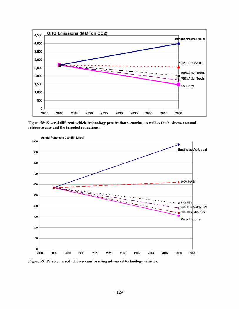
- 129 -

GHG Emissions (MMTon CO2)

0

500

1,000

1,500

2,000

2,500

3,000

3,500

4,000

4,500

2005 2010 2015 2020 2025 2030 2035 2040 2045 2050

Business-as-Usual

100% Future ICE

50% Adv. Tech.

550 PPM

75% Adv. Tech

Figure 58: Several different vehicle technology penetration scenarios, as well as the business-as-usual reference case and the targeted reductions.

Annual Petroleum Use (Bil. Liters)

0

100

200

300

400

500

600

700

800

900

1000

2000 2005 2010 2015 2020 2025 2030 2035 2040 2045 2050 2055

Zero Imports

75% HEV

100% NA-SI

Business-As-Usual

25% PHEV, 50% HEV

50% HEV, 25% FCV

Figure 59: Petroleum reduction scenarios using advanced technology vehicles.

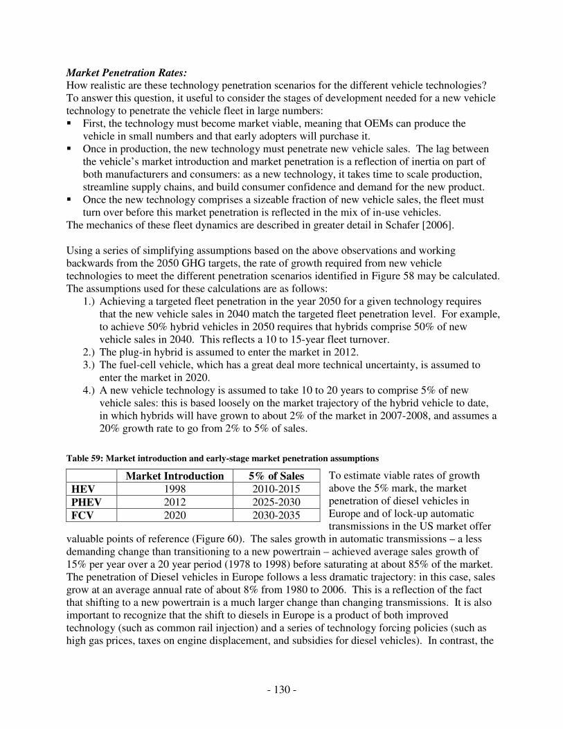
- 130 -

Market Penetration Rates: How realistic are these technology penetration scenarios for the different vehicle technologies? To answer this question, it useful to consider the stages of development needed for a new vehicle technology to penetrate the vehicle fleet in large numbers: First, the technology must become market viable, meaning that OEMs can produce the

vehicle in small numbers and that early adopters will purchase it. Once in production, the new technology must penetrate new vehicle sales. The lag between

the vehicle’s market introduction and market penetration is a reflection of inertia on part of both manufacturers and consumers: as a new technology, it takes time to scale production, streamline supply chains, and build consumer confidence and demand for the new product.

Once the new technology comprises a sizeable fraction of new vehicle sales, the fleet must turn over before this market penetration is reflected in the mix of in-use vehicles.

The mechanics of these fleet dynamics are described in greater detail in Schafer [2006]. Using a series of simplifying assumptions based on the above observations and working backwards from the 2050 GHG targets, the rate of growth required from new vehicle technologies to meet the different penetration scenarios identified in Figure 58 may be calculated. The assumptions used for these calculations are as follows:

1.) Achieving a targeted fleet penetration in the year 2050 for a given technology requires that the new vehicle sales in 2040 match the targeted fleet penetration level. For example, to achieve 50% hybrid vehicles in 2050 requires that hybrids comprise 50% of new vehicle sales in 2040. This reflects a 10 to 15-year fleet turnover.

2.) The plug-in hybrid is assumed to enter the market in 2012. 3.) The fuel-cell vehicle, which has a great deal more technical uncertainty, is assumed to

enter the market in 2020. 4.) A new vehicle technology is assumed to take 10 to 20 years to comprise 5% of new

vehicle sales: this is based loosely on the market trajectory of the hybrid vehicle to date, in which hybrids will have grown to about 2% of the market in 2007-2008, and assumes a 20% growth rate to go from 2% to 5% of sales.

Table 59: Market introduction and early-stage market penetration assumptions

To estimate viable rates of growth above the 5% mark, the market penetration of diesel vehicles in Europe and of lock-up automatic transmissions in the US market offer

valuable points of reference (Figure 60). The sales growth in automatic transmissions – a less demanding change than transitioning to a new powertrain – achieved average sales growth of 15% per year over a 20 year period (1978 to 1998) before saturating at about 85% of the market. The penetration of Diesel vehicles in Europe follows a less dramatic trajectory: in this case, sales grow at an average annual rate of about 8% from 1980 to 2006. This is a reflection of the fact that shifting to a new powertrain is a much larger change than changing transmissions. It is also important to recognize that the shift to diesels in Europe is a product of both improved technology (such as common rail injection) and a series of technology forcing policies (such as high gas prices, taxes on engine displacement, and subsidies for diesel vehicles). In contrast, the

Market Introduction 5% of Sales HEV 1998 2010-2015

PHEV 2012 2025-2030

FCV 2020 2030-2035

- 131 -

shift towards automatic transmissions was been driven purely by technological advances and market forces.

Market Penetration

0%

10%

20%

30%

40%

50%

60%

70%

80%

90%

100%

1975 1980 1985 1990 1995 2000 2005 2010

15% Annual Growth

8% Annual Growth

Diesel

Automatic Transmission

10% Annual Growth

Introduction of

Common-rail Injection

60% Annual Growth

Figure 60: Market penetration rates of different vehicle technologies. Source: Automatic transmission penetration data from EPA [2006a]; Diesel penetration data from ACEA [2007].

These historical examples give a sense of the difficulty in maintaining high growth rates once the technology has achieved a threshold level of market penetration. The 15% growth rate of automatic transmissions is likely unrealistic for a new powertrain technology once it has passed the 5% mark; this might be viewed as an upper-bound. The rapid growth of diesel vehicles in Europe is a reflection of the growth rate for a new powertrain that can be achieved through a combination of competitive technology and strong policy incentives. Of course, it must be recognized that for radically new vehicle technologies – particularly the fuel-cell – the magnitude of change in terms of vehicle technology, supply chain, and infrastructure is far outside the realm of experience. Using these observations, Table 60 shows the required growth rate in new vehicle sales required to meet different market penetration targets; the boxes are shaded according to the plausibility of the targeted market penetration scenarios. According to this analysis, the market penetration scenarios shown in Figure 58 and Figure 59 for the hybrid vehicle are all arguably plausible: assuming that sales reach 5% between 2010 and 2015, an annual sales rate of 6%-11% is needed to achieve market penetrations of 25% to 75% in the 2050 fleet. An aggressive plug-in hybrid penetration scenario is much more difficult: assuming it reaches 5% sales between 2025 and 2030, the plug-in hybrid would require 11% sales growth to achieve a 25% penetration target (plausible, but difficult); higher levels of market penetration are quite a bit more challenging.

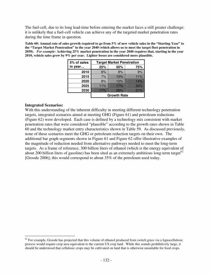
- 132 -

The fuel-cell, due to its long lead-time before entering the market faces a still greater challenge: it is unlikely that a fuel-cell vehicle can achieve any of the targeted market penetration rates during the time frame in question.

Table 60: Annual rate of sales growth required to go from 5% of new vehicle sales in the “Starting Year” to the “Target Market Penetration” in the year 2040 (which allows us to meet the target fleet penetration in 2050). For example: Achieving 25% market penetration in the year 2040 requires that, starting in the year 2010, vehicle sales grow by 9% per year. Lighter boxes are considered more plausible.

Target Market Penetration 5% of sales in year… 25% 50% 75%

2010 6% 8% 9%

2015 7% 10% 11%

2020 8% 12% 14%

2025 11% 17% 20%

2030 17% 26% 31%

Growth Rate

Integrated Scenarios: With this understanding of the inherent difficulty in meeting different technology penetration targets, integrated scenarios aimed at meeting GHG (Figure 61) and petroleum reductions (Figure 62) were developed. Each case is defined by a technology mix consistent with market penetration rates that were considered “plausible” according to the growth rates shown in Table 60 and the technology market entry characteristics shown in Table 59. As discussed previously, none of these scenarios meet the GHG or petroleum reduction targets on their own. The additional bar graph segments shown in Figure 61 and Figure 62 offer illustrative examples of the magnitude of reduction needed from alternative pathways needed to meet the long-term targets. As a frame of reference, 300 billion liters of ethanol (which is the energy equivalent of about 200 billion liters of gasoline) has been sited as an extremely ambitious long-term target62 [Groode 2006]; this would correspond to about 35% of the petroleum used today.

62 For example, Groode has projected that this volume of ethanol produced from switch grass via a lignocellulosic process would require crop area equivalent to the current US crop land. While this sounds prohibitively large, it should be understood that cellulosic crops may be cultivated on land that is otherwise unsuitable for food crops.

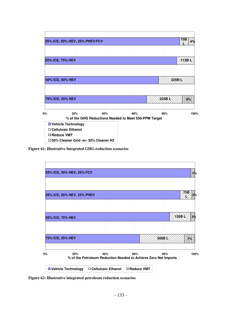
- 133 -

8%

4%

0% 20% 40% 60% 80% 100%

Vehicle Technology

Cellulosic Ethanol

Reduce VMT

50% Cleaner Grid -or- 30% Cleaner H2

25% ICE, 50% HEV, 25% PHEV/FCV

225B L

% of the GHG Reductions Needed to Meet 550-PPM Target

75% ICE, 25% HEV

50% ICE, 50% HEV

25% ICE, 75% HEV

75B

L

113B L

225B L

Figure 61: Illustrative Integrated GHG-reduction scenarios

7%

3%

3%

2%

0% 20% 40% 60% 80% 100%

Vehicle Technology Cellulosic Ethanol Reduce VMT

25% ICE, 50% HEV, 25% FCV

75B

L

% of the Petroleum Reduction Needed to Achieve Zero Net Imports

75% ICE, 25% HEV

25% ICE, 75% HEV

25% ICE, 50% HEV, 25% PHEV

135B L

300B L

Figure 62: Illustrative integrated petroleum reduction scenarios

- 134 -

While an evaluation of the relative difficulty in pursuing these different pathways – aggressive technology penetration, increasing the fraction of low-carbon domestic fuels, or demand-side reductions – is beyond the scope of this study, the key takeaway is that the magnitude of reduction required from other pathways varies considerably based on how successfully the new vehicle technologies penetrate the market. Each pathway becomes progressively more difficult as it is forced to bear a greater fraction of the burden, so an integrated approach will offer the least-cost, most robust path to achieving long-term targets.

9 Conclusions A broad theme of this study is that, while electric powertrains can make a valuable contribution to reducing one or both of petroleum consumption and GHG emissions in the long-run, they do not offer the prospect for solving these problems on their own. The results of the technology evaluation suggest that it is important not to overstate the near-term impact of deploying new vehicle technologies. This conclusion is based on the practical realities imposed both by the pace of technological development and by the time required to build production volume. Over the next several decades, conventional technologies – vehicles using a spark-ignition or diesel engine – are likely to continue to dominate the in-use vehicle fleet. As such, it is vital that technological development focus on improving the fuel efficiency of conventional technologies over this period. This conclusion is based on two factors:

1.) Because these technologies will comprise the bulk of vehicle-miles during this period (through 2030), near-term reductions in petroleum consumption and GHG emissions will need to come from improving conventional technologies, not from deploying new powertrains.

2.) Conventional technologies fix the performance and size characteristics of the in-use fleet. If vehicles continue to compete primarily on the basis of size and power, this will impact both conventional technology and the new entrants. In a related sense, improvements in the hybrid vehicle, and to a lesser extent, the plug-in hybrid, accrue relative to the spark-ignition engine.

Kasseris [2006] demonstrates that these conventional technologies have significant room to decrease fuel consumption, but only if vehicle technology improvements are used to improve on-the-road fuel consumption, rather than to power larger, more powerful cars (as has been the historic precedent). While conventional technology is likely to continue to dominate for the next two decades, continued technical development and increasing sales volume of hybrid vehicles are likely to drive down costs and improve performance. These improvements, in combination with aggressive policy measures to overcome consumer reluctance to pay a premium for high-efficiency vehicles, can bring the hybrid vehicle into the fleet in large numbers in the year 2030 and beyond. In this analysis, the hybrid vehicle plays a critical role as a bridging technology to transition from the near-term reliance on incremental efficiency improvements in conventional technology (and continued use of petroleum) to an eventual goal of non-GHG emitting, domestic transportation energy sources.

- 135 -

The evolution of battery and fuel-cell technology over the next 10-20 years will likely dictate whether the plug-in hybrid or the fuel-cell vehicle succeeds the hybrid vehicle. The plug-in hybrid, which has lower technical risk than the fuel-cell and addresses many of the shortcomings of the electric vehicle, may be deployed in low numbers in the next ten years; depending on consumer response, market drivers, and technical development, it might remain as a niche vehicle or grow into an increasing fraction of vehicle sales. Based on historical rates of change in the auto industry, it could comprise 25% of the cars on the road by mid-century. Over the long-term, the plug-in hybrid may bridge the way to a transportation system based either on battery-electric or on fuel-cell vehicles; alternatively, with successful deployment of bio-fuels at scale, it could form a long-term solution in its own right. In this sense, the plug-in hybrid offers a valuable “plan-B” if the other options do not pan out or develop too slowly. The fuel-cell, which faces significant technical and infrastructure hurdles, is likely to have minimal impact over the 30-year time horizon of this study, even with successful development. The electric powertrains evaluated are likely to cost several thousand dollars more than the conventional ICE-based technologies into the foreseeable future. Historically, consumers have been unwilling to pay a price premium for fuel efficiency; they are motivated instead by performance, comfort, and safety. As such, aggressively penetrating the market with high efficiency vehicles will require strong market drivers to overcome this reluctance: such drivers could include a system of fee-bates63 and fuel taxes64. It is also important to identify the advantages of new entrants and sell these vehicles on their own merits: for example, due to its high low-end torque and high efficiency across its operating range, an electric powertrain can deliver a vehicle that is both fun to drive and high-efficiency. Electric powertrains also offer additional benefits, such as silent operation and a portable electric power source. These are all attributes for which consumers could be willing to pay a price premium. To meet long-term targets, it is vital that, in parallel with aggressively pursuing efficiency improvements in vehicle technologies, domestic, non-GHG emitting fuel feedstocks and production processes be developed. This point is particularly compelling in light of the fact that the more futuristic powertrain options (the plug-in hybrid, the fuel-cell, and the electric vehicle) offer limited GHG reduction benefits over hybrid vehicles according to the base-case projections. In a similar vein, transitioning transportation energy from petroleum to natural gas (which, like petroleum, is subject to high price volatility and much of which is imported) does not necessarily solve energy security issues: hence, producing hydrogen or generating electricity from natural gas must be carefully evaluated in light of the over-arching goals in question. There is a temptation to assume that deploying new powertrains with low in-use emissions will solve the GHG problem on their own, but the reality is that developing clean fuel pathways will require extensive technological and infrastructure development in their own right. Electric powertrains offer the opportunity to achieve a step-change reduction in petroleum use and GHG emissions in the United States light-duty fleet. However, it will be several decades before these technologies can penetrate the in-use fleet and are likely to come at a higher cost

63 A fee-bate provides a purchase-time rebate for high-efficiency vehicles and purchase-time tax on low-efficiency vehicles. 64 CAFE standard increases are not included in this list because these act primarily to improve the fuel economy of the fleet average – they are less effective at driving the extremes of the market.

- 136 -

than conventional technologies. In addition, these technologies cannot meet long-term petroleum or GHG reduction targets by themselves. They must be deployed in combination with other aggressive measures such as improved conventional technology, development of low-carbon fuels and fuel production pathways, and demand-side reductions.

10 Recommendations

This study does not predict what will happen, but rather what could happen with aggressive, but realistic development and deployment of new vehicle technologies. The findings of this study suggest a number of broad-based strategic policy directions that will facilitate meeting long-term greenhouse gas and petroleum reduction targets. Pursue incremental improvements in conventional technologies in parallel with developing

new powertrain technologies. The expectation in both policy circles and the popular ideology is that new powertrain technologies can single-handedly solve the energy issues in the transportation sector. While developing these solutions is vital, it is important to recognize that these new entrants would be long-term solutions. Conventional powertrain technologies will comprise the major fraction of the in-use fleet for decades to come; in addition, the performance characteristics of conventional technologies will influence the characteristics of new technologies which must compete against them in the marketplace. The extent to which these factors are moderated in conventional technology will influence the energy use of new entrants.

Develop clean, domestic fuel pathways. The introduction of new powertrains into the market

will not meet long-term targets by itself; alternative powertrains offer only marginal GHG reduction benefits unless they are deployed in concert with greener fuel production pathways. In a similar vein, it is important to understand that transitioning from petroleum to transportation fuels sourced from natural gas may do little to alleviate energy security concerns.

Implement strong incentives to promote fuel efficiency: The cost of electric powertrains is

likely to be higher than that of conventional technologies. While they may offer some additional attractive attributes and lower operating cost, these factors alone may not motivate mass-market success. As such, it is likely that additional efficiency-forcing policies will be needed to help pull these technologies into the market.

Develop goal-based incentives aimed at deploying new technologies while continuing to

pursue development of critical enabling technologies. This technology assessment does not suggest a clear winner at this point amongst the different vehicle technologies: hybrid vehicles look promising in the near-term, but are constrained by their continued reliance on petroleum; and depending on technical development, either plug-in hybrids or fuel-cells could eventually become dominant players in the market. As such, it is important to work aggressively to develop both battery and fuel-cell technology and to develop goal-based, rather than technology-based incentives to promote efficiency.

- 137 -

References

A123 Website. www.a123.com. Accessed January 2007. ACEA. Diesel: Historical Series: 1990-2006 By Vehicle Category. February 2007. Available at http://www.acea.be/statistics. Accessed April 2007. Ahluwalia, R and X Wang. Direct Hydrogen Fuel Cell Systems for Hybrid Vehicles. Journal of Power Sources 139. 2005. Pp 152-164. An, Feng and DeCicco, John. Trends in Technical Efficiency Trade-Offs for the US Light Vehicle Fleet. SAE Technical Paper Series. SAE 2007-01-1325. April 2007. Anderman M, F Kalhammer, and D MacArthur. Advanced Batteries for Electric Vehicles: An Assessment of Performance, Cost, and Availability. California Air Resources Board, June 2000. Anderman, M. Brief Assessment of Improvements in EV Battery Technology Since the BTAP June 2000 Report. Agreement #02-611. California Air Resources Board (CARB). 2003. Anderman, M. The Ultracapacitor Opportunity Report. Advanced Automotive Batteries, February 2005. autos.com. www.autos.com. Accessed online database for various vehicle specifications. Ballard Power Systems. Ballard Power Systems – technology road map. Online at http://www.ballard.com/be_informed/fuel_cell_technology/roadmap, accessed May 2, 2007. Barsacq, Francois. Lithium-Ion Battery Overview for PHEV Applications. EPRI Workshop, April 3, 2005. Brodd, Ralph. Factors Affecting US Production Decisions: Why are There No Volume Lithium-Ion Battery Manufacturers in the United States? Prepared for National Institute of Standards, Contract SB 1341-02-W-1445. June 2005. Broussley, M et al. Main Aging Mechanisms in Li-Ion Batteries. Journal of Power Sources 146 (2005). Pp 90-96. Buchmann, Isidor. High Power Lithium-Iion, a New Area in Portable Power. March 2006. Viewed on the web at http://www.buchmann.ca/Article27-Page1.asp in 12/2006. Bullis, Kevin. Higher-Capacity Lithium-Ion Batteries. The Technology Review, June 2006. Available at http://www.technologyreview.com/Nanotech/17017/page1/. Bush, G. 2007 State of the Union Policy Initiatives – Twenty in Ten: Strengthening America’s Energy Security. January 2007. Available online at http://www.whitehouse.gov/stateoftheunion/2007/initiatives/energy.html, Accessed May 2, 2007.

- 138 -

Carlson, E, P Kopf, J Sinha, S Sriramulu. Cost Analysis of PEM Fuel Cell Systems for Transportation. National Renewable Energy Laboratory. Subcontract Report NREL/SR-560-39104. September 30, 2005. Chiang, Y. High Performance Batteries to Transform Transportation. Technology Review’s Emerging Technology Conference, 9/28/2006. Chu, A. Design Considerations and the Status and Future Plans for Lithium-ion Batteries Using Iron Phosphate in the Cathode. California Air Resources Board ZEV Symposium. September 27, 2006. CONCAWE, EUCAR, and ECJRC (EUWTW), Well-to-Wheels Analysis of Future Automotive Fuels and Powertrains in the European Context - Well-to Wheels Report, Version 2b. May 2006. Available at:http://ies.jrc.cec.eu.int/wtw.html Davis, Stacy and Diegel, Susan. Transportation Energy Data Book. Center for Transportation Analysis, Oak Ridge National Laboratory. 2004. Duleep, KG. Personal Correspondence. March 9, 2007. Duvall, M. Electricity as an Alternate Fuel: Re-thinking Off-Peak Charging. Plug-in Hybrid Electric Vehicle Workshop. Electric Power Research Institute (EPRI). November 15, 2003. Duvall, M. Plug-In Hybrid Electric Vehicle Intro and Battery Requirements. Presented at South Coast AQMD Plug-in Hybrid Electric Vehicle Forum and Technical Roundtable. July 12, 2006. EG&G Technical Services, Inc. Fuel Cell Handbook, 7th Edition. US Department of Energy, Office of Fossil Energy, National Energy Technology Laboratory. Contract DE-AM26-99FT40575. November 2004. Electric Power Research Institute (EPRI). Comparing the Benefits and Impacts of Hybrid Vehicle Options. EPRI, Palo Alto, CA. July 2001. Report 1000349. Energy Efficiency and Renewable Energy (EERE 2007a), US Department of Energy. The Partnership for a Next Generation of Vehicles. http://www.fueleconomy.gov/feg/pngv.shtml, accessed on 4/1/2007. Energy Efficiency and Renewable Energy (EERE 2007b), US Department of Energy. EERE: Freedom Car and Vehicle Technologies Homepage. http://www1.eere.energy.gov/vehiclesandfuels/, accessed on 4/1/2007. Energy and Environmental Analysis, Inc (EEA). Analysis and Forecast of the Performance and Cost of Conventional and Electric-Hybrid Vehicles. Contract No 500-00-002 (WA 8). March 2002.

- 139 -

Energy Information Administration (EIA), U.S. DOE. Annual Energy Outlook 2006. DOE/IEA-0383(2006). February 2006. Environmental Protection Agency (EPA 2002). eGRID2002 Version 2.01. EPA, 2002. Available online at http://www.epa.gov/solar/egrid/archive2002.htm, accessed 5/2/2007. Environmental Protection Agency (EPA 2006a). Light-Duty Automotive Technology and Fuel Economy Trends: 1975 Through 2005. EPA 420 R/06/011. Washington, D.C., July 2006. Environmental Protection Agency (EPA 2006b). Fuel Economy Labeling of Motor Vehicle Revisions to Imporve Calculation of Fuel Economy Estimates, Final Technical Support Document. EPA 420 R/06/017. December 2006. Farrington, R and J Rugh. Impact of Vehicle Air-Conditioning on Fuel Economy, Tailpipe Emissions, and Electric Vehicle Range. National Renewable Energy Laboratory. Contract No. DE-AC36-99-GO10337. October 2000. Frost, Jack. Hydrogen and Fuel Cells for Automotive Application. Presented at IMechE, London. November 7, 2006. Gaines, L and R Cuenca. Costs of Lithium-Ion Batteries for Vehicles. Center for Transportation Research, Energy Systems Division, Argonne National Laboratory. May 2000. Gasteiger, H, S Kocha, B Sompalli, F Wagner. Activity Benchmarks and Requirements for Pt, Pt-alloy, and non-Pt Oxygen Reduction Catalysts for PEMFCs. Applied Catalysis B: Environmental 56, 2005. Pp 9-35. General Motors, Argonne National Lab (GM/ANL), Well-to-Wheel Energy Use and Greenhouse Gas Emissions of Advanced Fuel/Vehicle Systems – North American Analysis, Vol. 2, http://www.transportation.anl.gov/software/GREET/publications.html. May 2005. Groode, T. A Methodology for Assessing MIT’s Energy Use and Greenhouse Gas Emissions. MSc. Thesis, Department of Mechanical Engineering, Massachusetts Institute of Technology. May 2004. Groode, T. Life Cycle and Impact Assessment of Ethanol from Various Biomass Sources. MIT/PSI Workshop, November 2006. Guzy, Chris. Fuel Cells for Transportation Applications. Presented at the CARB ZEV Symposium. Sept 25, 2006. Ballard Power Systems. Available online at http://www.arb.ca.gov/msprog/zevprog/symposium/presentations/presentations.htm. Gee, M. Cost and Performance Enhancements for a PEM Fuel Cell Turbocompressor. 2005 DOE Hydrogen Program Review Presentation. Project ID #FC27. May 25, 2005.

- 140 -

Green Car Congress. www.greencarcongress.com. Monthly updates on hybrid vehicle sales over the last several years were used. Green Car Congress (GCC). New PEM Membrane Material Retains Conductivity During Low Humidity. September 11, 2006. Available online at http://www.greencarcongress.com/2006/09/new_pem_membran.html. He, C, S Desai, G Brown, and S Bollepalli. “PEM Fuel Cell Catalysts: Cost, Performance, and Durability”. Electrochemical Society Interface, Fall 2005. Pp 41-44. House, Evan. Status of Lithium Batteries Using Lithium Titanate Based Anode. California Air Resources Board Zero-Emissions Vehicle Symposium. September 2006. Available at http://www.arb.ca.gov/msprog/zevprog/symposium/presentations/house.pdf. hybridcars.com. www.hybridcars.com. Accessed 3/1/2007. Intergovernmental Panel on Climate Change (IPCC). Climate Change 2007: The Physical Science Basis, Summary for Policymakers. February 2007. Kasseris, Emmanuel. Comparative Analysis of Automotive Powertrain Choices for the Near to Mid-Term Future. MSc. Thesis, Department of Mechanical Engineering, Massachusetts Institute of Technology, 2006. Keith, G, B Biewald, and D White. Displaced Emissions in Electric Power Systems: What Works and What Doesn’t. Synapse Energy Economics, prepared for the Commission for Environmental Cooperation. November 2004. Kleisch J, and T Langer. Plug-In Hybrids: An Environmental and Economic Performance Outlook. American Council for an Energy-Efficient Economy, Report T061. September 2006. Kintner-Meyer, M, K Schneider, and R Pratt. Impacts Assessment of Plug-in Hybrid Vehicles on Electric Utilities and Regional US Power Grids. Part 1: Technical Analysis. Department of Energy, Pacific Northwest National Laboratory (PNNL). Contract DE-AC05-76RL01830. December 2006. Kuuskraa, V, P DiPietro, and S Forbes. Technology Scenarios for Achieving Stabilization of Atmospheric GHG Concentrations: A US Perspective. 8th International Conference on Greenhouse Gas Control Technologies. June 19-22, 2006. Larminie, J and A Dicks. Fuel Cell Systems Explained, 2nd Edition. Wiley, 2003. Markel, T and A Simpson. Energy Storage Systems Considerations for Grid-Charged Hybrid Electric Vehicles. SAE Future Transportation Technology and IEEE Vehicle Power and Propulsion Joint Conferences. September 2005.

- 141 -

Markel, T. Plug-In HEV Vehicle Design Options and Expectations. California Air Resources Board ZEV Symposium. September 27, 2006. Online at http://www.arb.ca.gov/msprog/zevprog/symposium/presentations. Markel, Tony and Simpson, Andrew. Plug-In Hybrid Electric Vehicle Energy Storage System Design. Advanced Automotive Battery Conference. May 2006. Mathias, M, R Makharia, H Gasteiger, J Conley, T Fuller, C Gittleman, S Kocha, D Miller, C Mittelsteadt, T Xie, S Yan, and P Yu. Two Fuel Cells in Every Garage? Electrochemical Society Interface. Fall 2005. Pp 24-35. Miller, T. Hybrid Battery Technology and Challenges. Technology Review’s Emerging Technology Conference, 9/28/2006. Miller, T. Personal correspondence on 3/14/2007. Moon, P, Burnham, A, and Wang, M. Vehicle-Cycle Energy and Emissions Effects of Conventional and Advanced Vehicles. SAE Technical Paper Series. SAE 2006-01-0375. April 2006. Muta, K, M Yamazaki, and J Tokieda. Development of New-Generation Hybrid System THS II – Drastic Improvement of Power Performance and Fuel Economy. SAE Technical Paper Series. SAE 2004-01-0064. March 2004. Natarajan, Vinod. The Performance of IC Engine and Fuel Cell Hybrid Propulsion Systems in Light Duty Vehicles. MSc. Thesis, Department of Mechanical Engineering, Massachusetts Institute of Technology, 2002. National Research Council (NRC), Division of Earth and Life Sciences. Climate Change Science: An Analysis of Some Key Questions. Washington, D.C., 2001. National Research Council (NRC), Committee on Alternatives and Strategies for Future Hydrogen Production and Use. The Hydrogen Economy: Opportunities, Costs, Barriesr, and R&D Needs. Washington, D.C., 2004. 0-309-09163-2. National Research Council (NRC). Review of the Research Program of the FreedomCAR and Fuel Partnership. Washington, D.C., 2005. 0-309-09730-4. Nelson, D, and G Kulp. A Comparison of Two Fuel Cell Air Compression Systems at Low Load. SAE Technical Papers. SAE 2001-01-2547. August 2001. Northeast Advanced Vehicle Consortium (NAVC). Future Wheels II: A Survey of Expert Opinion on the Future of Transportation Fuel Cells. Northeast Advanced Vehicle Consortium. September 2003.

- 142 -

Obrovac, Mark. Advanced Materials for Lithium Ion Batteries. Presented at the Technology Review’s Emerging Technology Conference, 9/28/2006. Oak Ridge National Laboratory [ORNL]. 2001 National Household Travel Survey. Oak Ridge National Laboratory. January 2004. Online at http://nhts.ornl.gov/publications.shtml. Pew Climate Center. Renewable Map. Available at http://www.pewclimate.org/what_s_being_done/in_the_states/rps.cfm. Accessed 4/15/2007. Ritchie, Andrew. “Recent Developments and Likely Advances in Lithium-Ion Batteries”. Journal of Power Sources 136 (2004). Pp 285-289. Ritchie, Andrew and Howard, Wilmont. “Recent Developments and Likely Advances in Lithium-Ion Batteries”. Journal of Power Sources 162 (2006). Pp 809-812. Sadoway, Donald and Mayes, Anne. “Portable Power: Advanced Rechargeable Lithium Batteries”. MRS Bulleton, August 2002. Pp 590-596. SAE J1711 Technical Standard. Recommended Practice for Measuring the Exhaust Emissions and Fuel Economy of Hybrid-Electric Vehicles. Society of Automotive Engineers. March 1999 Standards. Saft Website. www.saftbatteries.com. Accessed 10/2006. Schafer, A, J Heywood, M Weiss. Future Fuel Cell and Internal Combustion Engine Automobile Technologies: A 25-year Life Cycle and Fleet Impact Assessment. Energy, Vol 31, Issue 12. September 2006. Pp 2064-2087. Schlapbach, L and A Zuttel. Hydrogen Storage Materials for Mobile Applications. Nature 414: 353-358. 2001. Sperling, Daniel. Transportation Energy Sustainability. TRB/NRC Conference on Transport Sustainability, July 2004. http://www.trb.org/conferences/sustainability/Sperling.pdf, accessed 4/27/2007. Srinivasan, Venkat and Newman, John. Design and Optimization of a Natural Graphite/Iron Phosphate Lithium-Ion Cell. Journal of the Electrochemical Society 151, No 10(2004). Pp A1530-A1538. Stamenkovic, V B Fowler, B Mun, G Wang, P Ross, C Lucas. Improvied Oxygen Reduction Activitiy on Pt3Ni(111) via Increased Surface Site Availability. Science, Vol 315, No 5811. January 26, 2007. Pp 493-497. Steinbugler, Margaret. PEM Fuel Cell Technology Readiness for Light Duty Vehicles. Presented at the CARB ZEV Symposium. Sept 25, 2006. UTC Fuel Cells. Available online at http://www.arb.ca.gov/msprog/zevprog/symposium/presentations/presentations.htm.

- 143 -

Thackeray, Michael. An Unexpected Conductor. Nature Materials, October 2002. Pp 81-82. http://libattery.ustc.edu.cn/english/introduction%203.htm, accessed 1/9/2007. Tiax. DOE Compress/Expander Module Development Program Merit Review Meeting. Tiax LLC. Reference DE-FC04-01AL67603. May 22, 2003. Wall, E. Consumer Perspectives Are Changing: Initial Resutls from ORC Survey on PHEVs. FreedomCAR and Vehicle Technologies Program, DOE Energy Efficiency & Renewable Energy. May 4, 2006. Ward’s motor vehicle facts and figures 2005, available at http://www.wardsauto.com/ Weiss M. A., J.B. Heywood, E.M. Drake, A. Schafer, and F. AuYeung, On the Road in 2020: A life-cycle Analysis of New Automobile Technologies, MIT Laboratory for Energy and the Environment Report, MIT EL 00-003, October 2000. Weiss M.A., J.B. Heywood, A. Schafer, and V.K. Natarajan, Comparative Assessment of Fuel Cell Cars, MIT Laboratory For Energy and the Environment Report, MIT LFEE 2003-001 RP. World Business Council for Sustainable Development. Mobility 2030: Meeting the Challenges to Sustainability. The Sustainability Mobility Project, 2004. Zhang, J, K Sasaki, E Sutter, and R Adzic. Stabilization of Platinum Oxygen-Reduction Electrocatalysts Using Gold Clusters. Science Vol 315, No 5809. January 12, 2007. Pp 220-222. Zhou, Z, S Li, Y Zhang, M Li, W Li. Promotion of Proton Conduction in Polymer Electrolyte Membranes by 1H-1,2,3-Triazole. Journal of the American Chemical Society 172(31). 2005. Pp 10824-10825.

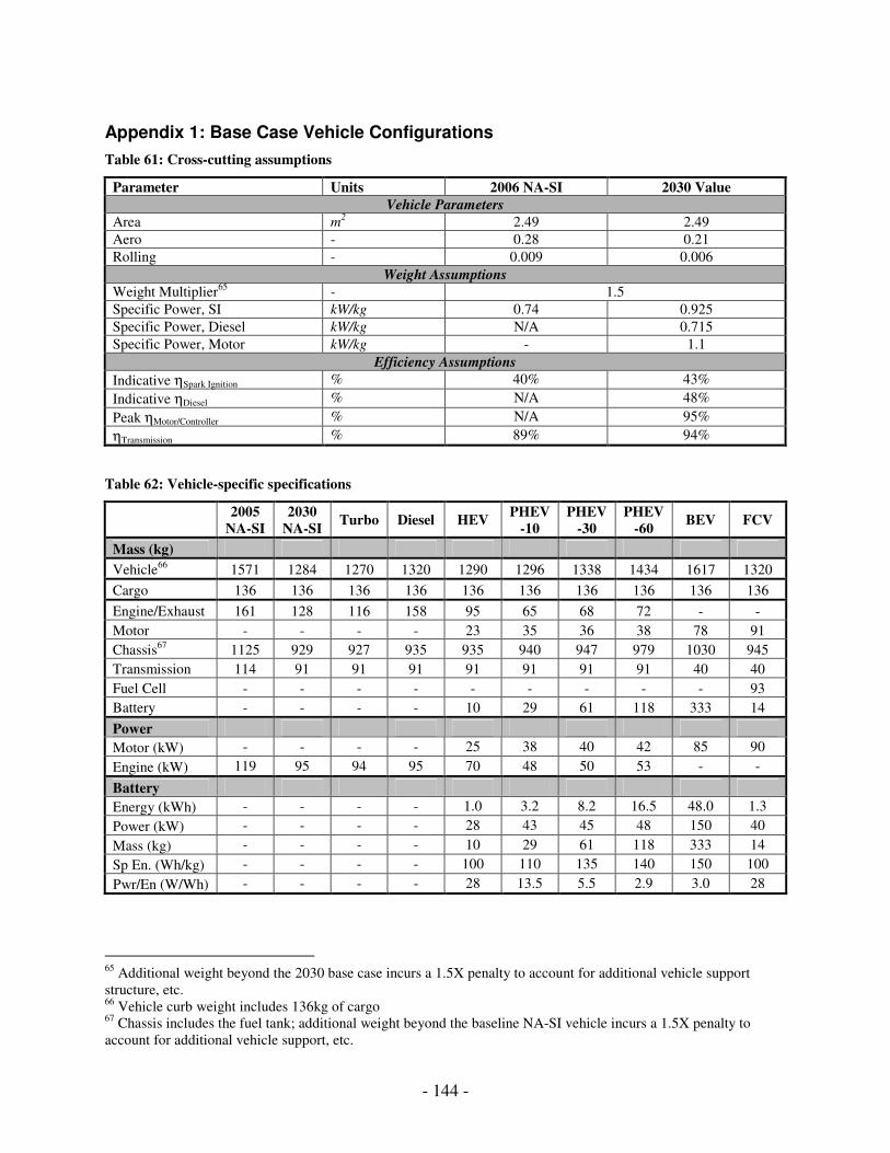
- 144 -

Appendix 1: Base Case Vehicle Configurations

Table 61: Cross-cutting assumptions

Parameter Units 2006 NA-SI 2030 Value Vehicle Parameters

Area m2 2.49 2.49

Aero - 0.28 0.21

Rolling - 0.009 0.006

Weight Assumptions

Weight Multiplier65 - 1.5

Specific Power, SI kW/kg 0.74 0.925

Specific Power, Diesel kW/kg N/A 0.715

Specific Power, Motor kW/kg - 1.1

Efficiency Assumptions

Indicative ηSpark Ignition % 40% 43%

Indicative ηDiesel % N/A 48%

Peak ηMotor/Controller % N/A 95%

ηTransmission % 89% 94%

Table 62: Vehicle-specific specifications

2005

NA-SI 2030

NA-SI Turbo Diesel HEV

PHEV-10

PHEV-30

PHEV-60

BEV FCV

Mass (kg)

Vehicle66 1571 1284 1270 1320 1290 1296 1338 1434 1617 1320

Cargo 136 136 136 136 136 136 136 136 136 136

Engine/Exhaust 161 128 116 158 95 65 68 72 - -

Motor - - - - 23 35 36 38 78 91

Chassis67 1125 929 927 935 935 940 947 979 1030 945

Transmission 114 91 91 91 91 91 91 91 40 40

Fuel Cell - - - - - - - - - 93

Battery - - - - 10 29 61 118 333 14

Power

Motor (kW) - - - - 25 38 40 42 85 90

Engine (kW) 119 95 94 95 70 48 50 53 - -

Battery

Energy (kWh) - - - - 1.0 3.2 8.2 16.5 48.0 1.3

Power (kW) - - - - 28 43 45 48 150 40

Mass (kg) - - - - 10 29 61 118 333 14

Sp En. (Wh/kg) - - - - 100 110 135 140 150 100

Pwr/En (W/Wh) - - - - 28 13.5 5.5 2.9 3.0 28

65 Additional weight beyond the 2030 base case incurs a 1.5X penalty to account for additional vehicle support structure, etc. 66 Vehicle curb weight includes 136kg of cargo 67 Chassis includes the fuel tank; additional weight beyond the baseline NA-SI vehicle incurs a 1.5X penalty to account for additional vehicle support, etc.

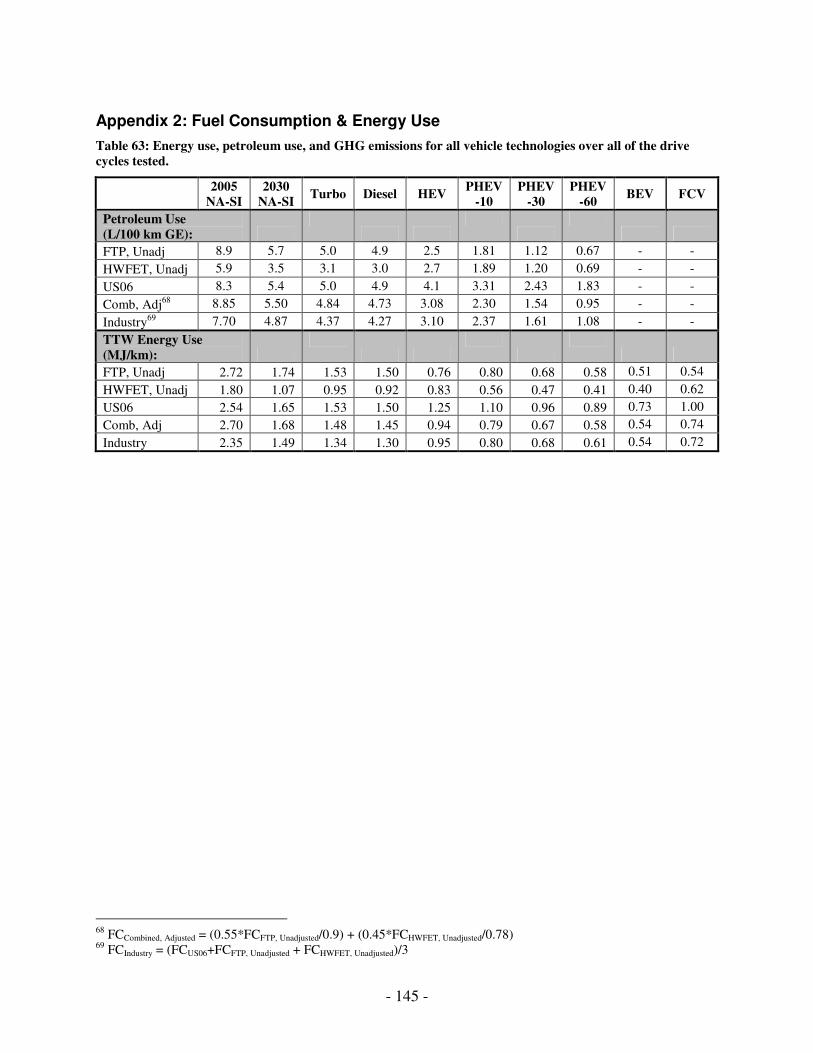
- 145 -

Appendix 2: Fuel Consumption & Energy Use

Table 63: Energy use, petroleum use, and GHG emissions for all vehicle technologies over all of the drive cycles tested.

2005

NA-SI 2030

NA-SI Turbo Diesel HEV

PHEV-10

PHEV-30

PHEV-60

BEV FCV

Petroleum Use (L/100 km GE):

FTP, Unadj 8.9 5.7 5.0 4.9 2.5 1.81 1.12 0.67 - -

HWFET, Unadj 5.9 3.5 3.1 3.0 2.7 1.89 1.20 0.69 - -

US06 8.3 5.4 5.0 4.9 4.1 3.31 2.43 1.83 - -

Comb, Adj68 8.85 5.50 4.84 4.73 3.08 2.30 1.54 0.95 - -

Industry69 7.70 4.87 4.37 4.27 3.10 2.37 1.61 1.08 - -

TTW Energy Use (MJ/km):

FTP, Unadj 2.72 1.74 1.53 1.50 0.76 0.80 0.68 0.58 0.51 0.54

HWFET, Unadj 1.80 1.07 0.95 0.92 0.83 0.56 0.47 0.41 0.40 0.62

US06 2.54 1.65 1.53 1.50 1.25 1.10 0.96 0.89 0.73 1.00

Comb, Adj 2.70 1.68 1.48 1.45 0.94 0.79 0.67 0.58 0.54 0.74

Industry 2.35 1.49 1.34 1.30 0.95 0.80 0.68 0.61 0.54 0.72

68 FCCombined, Adjusted = (0.55*FCFTP, Unadjusted/0.9) + (0.45*FCHWFET, Unadjusted/0.78) 69 FCIndustry = (FCUS06+FCFTP, Unadjusted + FCHWFET, Unadjusted)/3

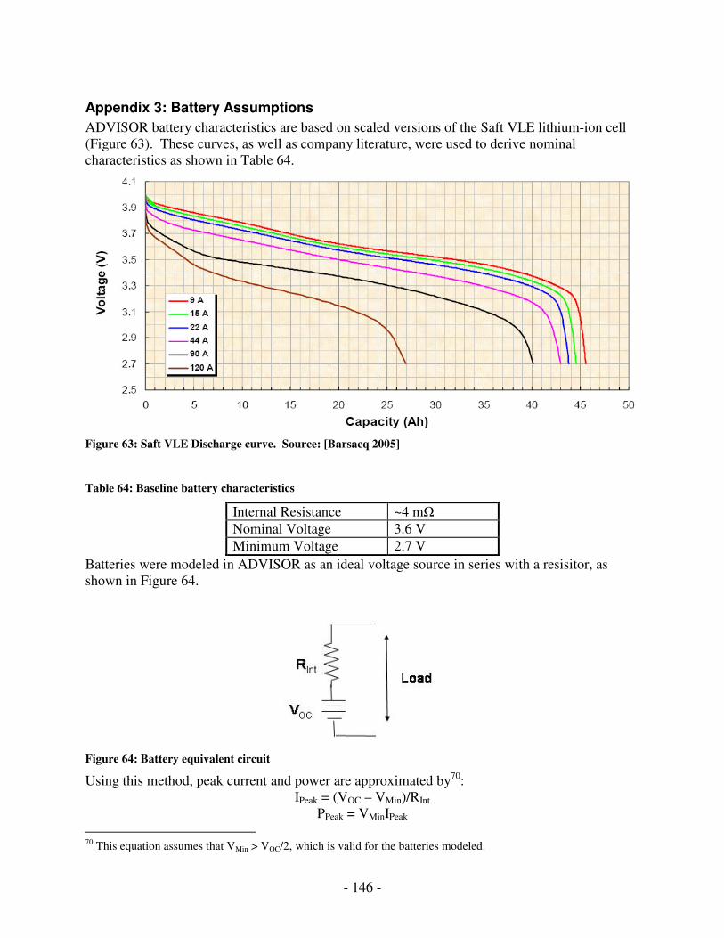
- 146 -

Appendix 3: Battery Assumptions

ADVISOR battery characteristics are based on scaled versions of the Saft VLE lithium-ion cell (Figure 63). These curves, as well as company literature, were used to derive nominal characteristics as shown in Table 64.

Figure 63: Saft VLE Discharge curve. Source: [Barsacq 2005]

Table 64: Baseline battery characteristics

Internal Resistance ~4 mΩ

Nominal Voltage 3.6 V

Minimum Voltage 2.7 V

Batteries were modeled in ADVISOR as an ideal voltage source in series with a resisitor, as shown in Figure 64.

Figure 64: Battery equivalent circuit

Using this method, peak current and power are approximated by70: IPeak = (VOC – VMin)/RInt

PPeak = VMinIPeak

70 This equation assumes that VMin > VOC/2, which is valid for the batteries modeled.

- 147 -

To scale battery energy and power to the appropriate future vehicle-specific energy, power, and weight characteristics, the following procedure was used:

1.) Calculate the number of cells needed to meet the required peak power 2.) Adjust the cell capacity to provide the required battery energy 3.) Adjust the vehicle/battery mass to meet the specified energy & power.

Strictly speaking, this method does not capture all of the differences between high energy and high power batteries, but additional sensitivity analysis using different battery maps derived from different chemistries did not show vary the results by a significant amount.

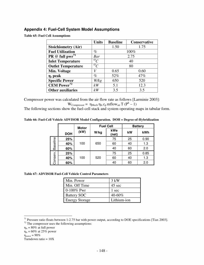
- 148 -

Appendix 4: Fuel-Cell System Model Assumptions

Table 65: Fuel Cell Assumptions

Units Baseline Conservative Stoichiometry (Air) 1.50 1.75

Fuel Utilization % 100%

PR @ full pwr71 Bar 2.75

Inlet Temperature OC 40

Outlet Temperature OC 80

Min. Voltage V 0.65 0.60

η, peak % 52% 47%

Specific Power W/kg 650 520

CEM Power72 kW 5.1 12.3

Other auxiliaries kW 3.5 3.5

Compressor power was calculated from the air flow rate as follows [Larminie 2003]:

WCompressor = ηMech ηIs cp mflowair T (Pk – 1) The following sections show the fuel-cell stack and system operating maps in tabular form.

Table 66: Fuel-Cell Vehicle ADVISOR Model Configuration. DOH = Degree-of-Hybridization

Fuel Cell Battery

DOH

Motor (kW) W/kg

kWe (net)

kW kWh

25% 75 25 0.90

40% 60 40 1.3

Baselin

e

60%

100 650

40 60 2.0

25% 75 25 0.85

40% 60 40 1.3

Conserv

.

60%

100 520

40 60 2.0

Table 67: ADVISOR Fuel-Cell Vehicle Control Parameters

Min. Power 3 kW

Min. Off Time 45 sec

0-100% Pwr 1 sec

Battery SOC 40-60%

Energy Storage Lithium-ion

71 Pressure ratio floats between 1-2.75 bar with power output, according to DOE specifications [Tiax 2003]. 72 The compressor uses the following assumptions: ηIs = 80% at full power ηIs = 60% at 25% power ηmotor = 90% Turndown ratio = 10X

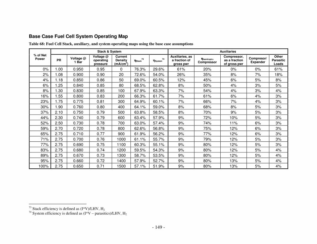
- 149 -

Base Case Fuel Cell System Operating Map

Table 68: Fuel Cell Stack, auxiliary, and system operating maps using the base case assumptions

Stack & System Auxiliaries % of Net Power PR

Voltage @ 1 Bar

Voltage @ operating pressure

Current Density

(mA/cm2)

ηηηηStack73

ηηηηSystem74

Auxiliaries, as a fraction of gross pwr

ηηηηIsentropic, Compressor

Compressor, as a fraction of gross pwr

Compresor/ Expander

Other Parasitic

Loads

0% 1.00 0.950 0.95 0 76.3% 29.6% 61% 20% 0% 0% 61%

2% 1.08 0.900 0.90 20 72.6% 54.0% 26% 35% 8% 7% 18%

4% 1.18 0.850 0.86 50 69.0% 60.5% 12% 45% 6% 5% 8%

6% 1.25 0.840 0.85 80 68.5% 62.8% 8% 50% 4% 3% 5%

8% 1.30 0.830 0.85 100 67.9% 63.3% 7% 54% 4% 3% 4%

16% 1.55 0.800 0.83 200 66.3% 61.7% 7% 61% 6% 4% 3%

23% 1.75 0.775 0.81 300 64.9% 60.1% 7% 66% 7% 4% 3%

30% 1.90 0.760 0.80 400 64.1% 59.0% 8% 68% 8% 5% 3%

37% 2.10 0.750 0.79 500 63.8% 58.5% 8% 70% 9% 5% 3%

44% 2.30 0.740 0.79 600 63.4% 57.9% 9% 72% 10% 5% 3%

52% 2.50 0.730 0.78 700 63.0% 57.4% 9% 74% 11% 6% 3%

59% 2.70 0.720 0.78 800 62.6% 56.8% 9% 75% 12% 6% 3%

65% 2.75 0.710 0.77 900 61.9% 56.2% 9% 77% 12% 6% 3%

71% 2.75 0.700 0.76 1000 61.1% 55.7% 9% 79% 12% 5% 3%

77% 2.75 0.690 0.75 1100 60.3% 55.1% 9% 80% 12% 5% 3%

83% 2.75 0.680 0.74 1200 59.5% 54.3% 9% 80% 12% 5% 4%

89% 2.75 0.670 0.73 1300 58.7% 53.5% 9% 80% 12% 5% 4%

95% 2.75 0.660 0.72 1400 57.9% 52.7% 9% 80% 13% 5% 4%

100% 2.75 0.650 0.71 1500 57.1% 51.9% 9% 80% 13% 5% 4%

73 Stack efficiency is defined as (I*V)/LHV, H2 74 System efficiency is defined as (I*V – parasitics)/LHV, H2

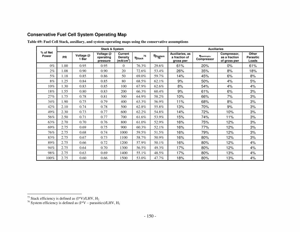
- 150 -

Conservative Fuel Cell System Operating Map

Table 69: Fuel Cell Stack, auxiliary, and system operating maps using the conservative assumptions

Stack & System Auxiliaries % of Net Power PR

Voltage @ 1 Bar

Voltage @ operating pressure

Current Density

(mA/cm2)

ηηηηStack75

ηηηηSystem

76

Auxiliaries, as a fraction of gross pwr

ηηηηIsentropic, Compressor

Compressor, as a fraction of gross pwr

Other Parasitic

Loads

0% 1.00 0.95 0.95 0 76.3% 29.6% 61% 20% 0% 61%

2% 1.08 0.90 0.90 20 72.6% 53.4% 26% 35% 8% 18%

5% 1.18 0.85 0.86 50 69.0% 59.7% 14% 45% 6% 8%

8% 1.25 0.84 0.85 80 68.5% 62.1% 9% 50% 4% 5%

10% 1.30 0.83 0.85 100 67.9% 62.6% 8% 54% 4% 4%

18% 1.55 0.80 0.83 200 66.3% 60.4% 9% 61% 6% 3%

27% 1.75 0.78 0.81 300 64.9% 58.2% 10% 66% 7% 3%

34% 1.90 0.75 0.79 400 63.3% 56.9% 11% 68% 8% 3%

42% 2.10 0.74 0.78 500 62.8% 55.8% 13% 70% 9% 3%

49% 2.30 0.73 0.77 600 62.2% 54.8% 14% 72% 10% 3%

56% 2.50 0.71 0.77 700 61.6% 53.9% 15% 74% 11% 3%

63% 2.70 0.70 0.76 800 61.0% 52.9% 16% 75% 12% 3%

69% 2.75 0.69 0.75 900 60.3% 52.1% 16% 77% 12% 3%

76% 2.75 0.68 0.74 1000 59.5% 51.5% 16% 79% 12% 3%

83% 2.75 0.67 0.73 1100 58.7% 50.9% 16% 80% 12% 3%

89% 2.75 0.66 0.72 1200 57.9% 50.1% 16% 80% 12% 4%

94% 2.75 0.64 0.70 1300 56.5% 49.3% 17% 80% 12% 4%

98% 2.75 0.63 0.69 1400 55.1% 48.5% 17% 80% 13% 4%

100% 2.75 0.60 0.66 1500 53.0% 47.7% 18% 80% 13% 4%

75 Stack efficiency is defined as (I*V)/LHV, H2 76 System efficiency is defined as (I*V – parasitics)/LHV, H2

- 151 -

Appendix 5: Plug-In Hybrid Configuration, Calculations, and Results

Total fuel consumption in the plug-in hybrid vehicle is calculated as follows:

FCtotal = (FCChg Depleting)(UF) + (FCChg Sustaining)(1-UF) Energy use in the plug-in hybrid vehicle is calculated as follows:

Energytotal = (EnergyChg Depleting)(UF) + (EnergyChg Sustaining)(1-UF) Charge depleting range is calculated from:

ElectricityChg Depleting = EnergyChg Depleting- FCChg Depleting

RangeChg Depleting = (Battery Energy) (ElectricityChg Depleting) (SOC Envelope)

Table 70: Plug-In Hybrid Simulation results

FTP,

Unadjusted HWY,

Unadjusted US06

Combined, Adjusted

Industry

Chg Sustaining (L/100 km)

PHEV-10 2.44 2.56 3.93 2.97 2.98

PHEV-30 2.54 2.62 3.89 3.07 3.02

PHEV-60 2.67 2.71 4.05 3.19 3.14

Chg Depleting, Petroleum (L/100 km)

PHEV-10 0.00 0.00 0.65 0.00 0.22

PHEV-30 0.00 0.00 0.59 0.00 0.20

PHEV-60 0.00 0.00 0.71 0.00 0.24

Chg Depleting, Energy (L/100 km, GE)

PHEV-10 1.05 1.11 2.18 1.29 1.45

PHEV-30 1.08 1.13 2.19 1.31 1.47

PHEV-60 1.13 1.16 2.32 1.36 1.54

Electricity Used (W-hr/Mi)

PHEV-10 150 158 217 193 175

PHEV-30 153 161 226 186 180

PHEV-60 161 165 228 183 185

Chg Depleting Range (Mi)77

PHEV-10 12.8 12.1 8.9 10.5 11.0

PHEV-30 37.7 35.9 25.4 31.0 32.0

PHEV-60 76.9 74.9 54.0 63.9 66.9

Utility Factor78

PHEV-10 0.26 0.26 0.66 0.22 0.39

PHEV-30 0.56 0.54 0.44 0.50 0.51

PHEV-60 0.75 0.74 0.19 0.70 0.56

77 Defined as the range that vehicle can travel from its maximum to minimum state-of-charge threshold 78 Utility Factor is the estimated fraction of vehicle miles traveled in charge-depleting mode.

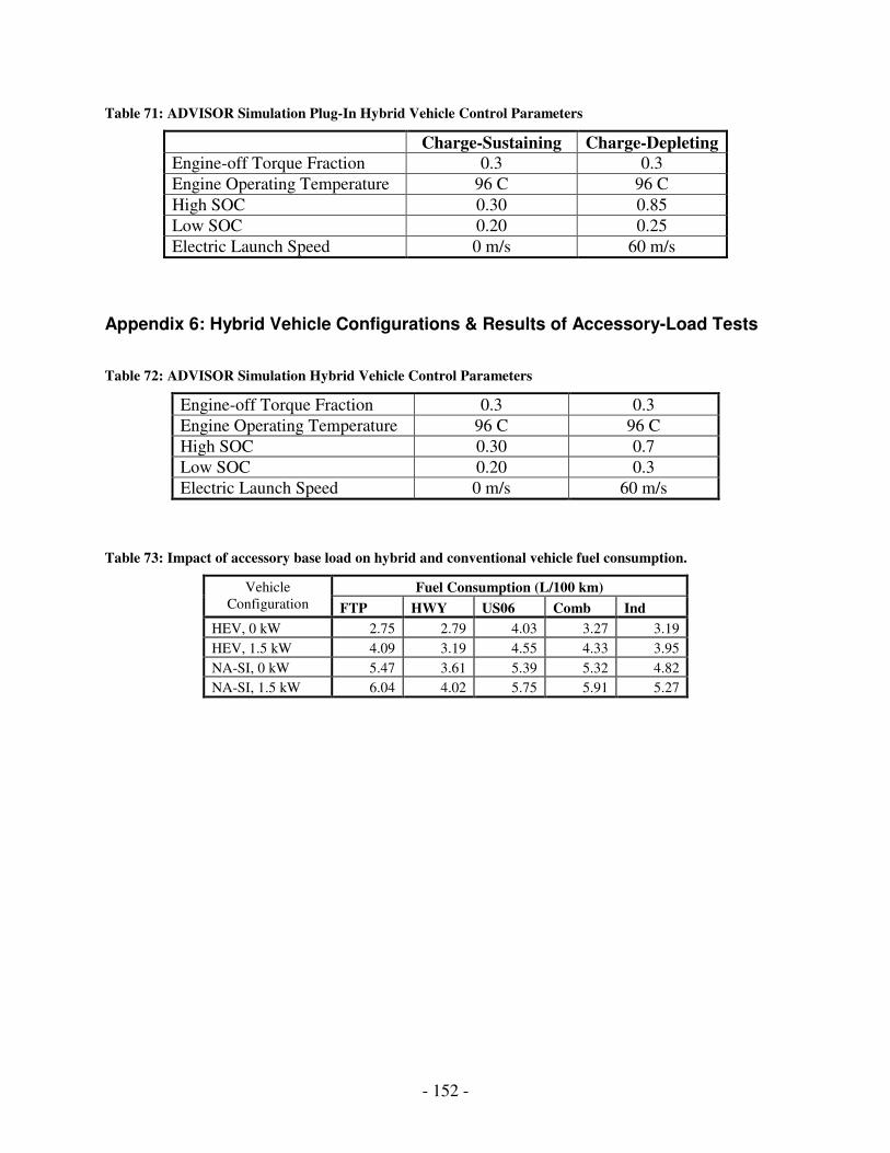
- 152 -

Table 71: ADVISOR Simulation Plug-In Hybrid Vehicle Control Parameters

Charge-Sustaining Charge-Depleting Engine-off Torque Fraction 0.3 0.3

Engine Operating Temperature 96 C 96 C

High SOC 0.30 0.85

Low SOC 0.20 0.25

Electric Launch Speed 0 m/s 60 m/s

Appendix 6: Hybrid Vehicle Configurations & Results of Accessory-Load Tests

Table 72: ADVISOR Simulation Hybrid Vehicle Control Parameters

Engine-off Torque Fraction 0.3 0.3

Engine Operating Temperature 96 C 96 C

High SOC 0.30 0.7

Low SOC 0.20 0.3

Electric Launch Speed 0 m/s 60 m/s

Table 73: Impact of accessory base load on hybrid and conventional vehicle fuel consumption.

Fuel Consumption (L/100 km) Vehicle Configuration FTP HWY US06 Comb Ind

HEV, 0 kW 2.75 2.79 4.03 3.27 3.19

HEV, 1.5 kW 4.09 3.19 4.55 4.33 3.95

NA-SI, 0 kW 5.47 3.61 5.39 5.32 4.82

NA-SI, 1.5 kW 6.04 4.02 5.75 5.91 5.27

- 153 -

Appendix 7: Definition of Vehicle Technologies

Hybrid-Electric Vehicle (HEV): A vehicle that integrates a gasoline-powered engine with an onboard electrical energy storage system to deliver motive power to the wheels. In a hybrid-electric vehicle, the primary energy is sourced from gasoline. Plug-in hybrid-electric vehicle (PHEV): A vehicle that uses both gasoline and off-board electricity to deliver motive power. In charge-depleting mode, the PHEV draws energy primarily from the battery; once the battery state-of-charge is depleted, it switches to charge-sustaining mode, in which primary energy is sourced from gasoline. “PHEV-XX” refers to a plug-in hybrid with a given electric range; for example a “PHEV-30” is estimated to have a 30 mile electric range. Battery-electric vehicle (also “Electric Vehicle”) (BEV): A vehicle that receives all motive power from off-board electricity. Fuel-Cell Vehicle (FCV): A vehicle that uses a proton-exchange membrane (PEM) fuel cell powered by stored onboard hydrogen to generate electricity.