Electric and Magnetic Response Properties of...

Electric and Magnetic Response Properties of Topological Insulatorsin Two and Three Dimensions

by

Andrew Michael Essin

A dissertation submitted in partial satisfaction of the

requirements for the degree of

Doctor of Philosophy

in

Physics

in the

Graduate Division

of the

University of California, Berkeley

Committee in charge:

Professor Joel E. Moore, Chair

Professor Ashvin Vishwanath

Professor Yuri Suzuki

Spring 2010


Copyright 2010

by


1

Abstract1


by


Doctor of Philosophy in Physics

University of California, Berkeley

Professor Joel E. Moore, Chair

This dissertation introduces some basic characteristics of a class of materials known astopological insulators. These materials were introduced theoretically as crystalline bandinsulators, in which electrons do not interact with each other and the atomic cores forma perfectly ordered, fixed background potential for the electrons. It is shown that, in thetwo-dimensional case, this definition can be relaxed to the case of disordered, noninteractinginsulators. It is further shown numerically that the introduction of disorder to these two-dimensional insulators eliminates the direct transition between the topological and ordinaryinsulating phases, consistent with the presence of an intervening metallic phase.

In the three-dimensional case, one formulation of the distinction between the topologicaland ordinary phases involves a quantized response function (the magnetoelectric polarizabil-ity). It is shown here that this characterization holds on quite general grounds, and thereforeallows an extension of the topological class to disordered and interacting systems. Finally,a relatively rigorous derivation of the (fixed-ion, linear, orbital) magnetoelectric response ofcrystalline band insulators is presented.

1 Yes, but some parts are reasonably concrete.— Avron et al., Commun. Math. Phys. 123, 595 (1989)

i

Contents

List of Figures iii

List of Tables iv

Acknowledgments v

1 Background and overview 11.1 Band theory of solids . . . . . . . . . . . . . . . . . . . . . . . . . . . . . . 11.2 Insulators, metals, and quasiparticles . . . . . . . . . . . . . . . . . . . . . . 31.3 Topological properties . . . . . . . . . . . . . . . . . . . . . . . . . . . . . . 41.4 The quantum Hall effect . . . . . . . . . . . . . . . . . . . . . . . . . . . . . 51.5 Topological insulators with time reversal symmetry . . . . . . . . . . . . . . 61.6 Outline . . . . . . . . . . . . . . . . . . . . . . . . . . . . . . . . . . . . . . . 8

2 Technical review and introduction 112.1 Insulators . . . . . . . . . . . . . . . . . . . . . . . . . . . . . . . . . . . . . 112.2 Adiabatic conduction, charge pumping, and geometry . . . . . . . . . . . . . 132.3 Electronic polarization (and magnetization) . . . . . . . . . . . . . . . . . . 172.4 Bloch’s theorem . . . . . . . . . . . . . . . . . . . . . . . . . . . . . . . . . . 172.5 Adiabatic conduction and geometry revisited, with projectors . . . . . . . . 19

3 Topological insulators with disorder and a spin-orbit metal 233.1 Introduction . . . . . . . . . . . . . . . . . . . . . . . . . . . . . . . . . . . . 233.2 Chern parities for disordered noninteracting electron systems . . . . . . . . . 28

3.2.1 The definition of the Z2 invariant in clean systems . . . . . . . . . . . 283.2.2 The topological insulator phase for Slater determinants via Chern parity 303.2.3 Charge pumping cycles in time-reversal-invariant systems . . . . . . . 32

3.3 Graphene Model and Numerics . . . . . . . . . . . . . . . . . . . . . . . . . 353.3.1 The phase diagram of the disordered graphene model . . . . . . . . . 353.3.2 Lattice Implementation . . . . . . . . . . . . . . . . . . . . . . . . . . 353.3.3 Numerical Results . . . . . . . . . . . . . . . . . . . . . . . . . . . . 37

3.4 Summary . . . . . . . . . . . . . . . . . . . . . . . . . . . . . . . . . . . . . 43

ii

4 Magnetoelectric polarizability and axion electrodynamics in crystalline in-sulators 45

Interlude: magnetoelectric response of a finite material 52

5 General orbital magnetoelectric coupling in band insulators 555.1 Introduction . . . . . . . . . . . . . . . . . . . . . . . . . . . . . . . . . . . . 555.2 General features of the orbital magnetoelectric response . . . . . . . . . . . . 58

5.2.1 The OMP expression and the origin of the cross-gap term αG . . . . 585.2.2 The Chern-Simons form, axion electrodynamics, and topological insu-

lators . . . . . . . . . . . . . . . . . . . . . . . . . . . . . . . . . . . . 595.2.3 Conditions causing αG to vanish . . . . . . . . . . . . . . . . . . . . . 625.2.4 Is the Chern-Simons contribution physically distinct? . . . . . . . . . 64

5.3 The OMP as the current in response to a chemical change . . . . . . . . . . 665.3.1 Single-body operators for a uniform magnetic field . . . . . . . . . . . 685.3.2 The ground state density operator . . . . . . . . . . . . . . . . . . . . 695.3.3 Adiabatic current . . . . . . . . . . . . . . . . . . . . . . . . . . . . . 71

5.4 Summary . . . . . . . . . . . . . . . . . . . . . . . . . . . . . . . . . . . . . 75

6 Conclusion 76

Bibliography 80

A Analogies between polarization and orbital magnetoelectric polarizability 88

B Calculating the OMP using static polarization 89

iii

List of Figures

1.1 Bands from atomic limit . . . . . . . . . . . . . . . . . . . . . . . . . . . . . 21.2 Generic metallic dispersion . . . . . . . . . . . . . . . . . . . . . . . . . . . . 31.3 Chiral edge state of quantum Hall effect . . . . . . . . . . . . . . . . . . . . 61.4 Edge states of 2D topological insulator . . . . . . . . . . . . . . . . . . . . . 71.5 Surface states of 3D topological insulator . . . . . . . . . . . . . . . . . . . . 8

2.1 Flux through a ring . . . . . . . . . . . . . . . . . . . . . . . . . . . . . . . . 11

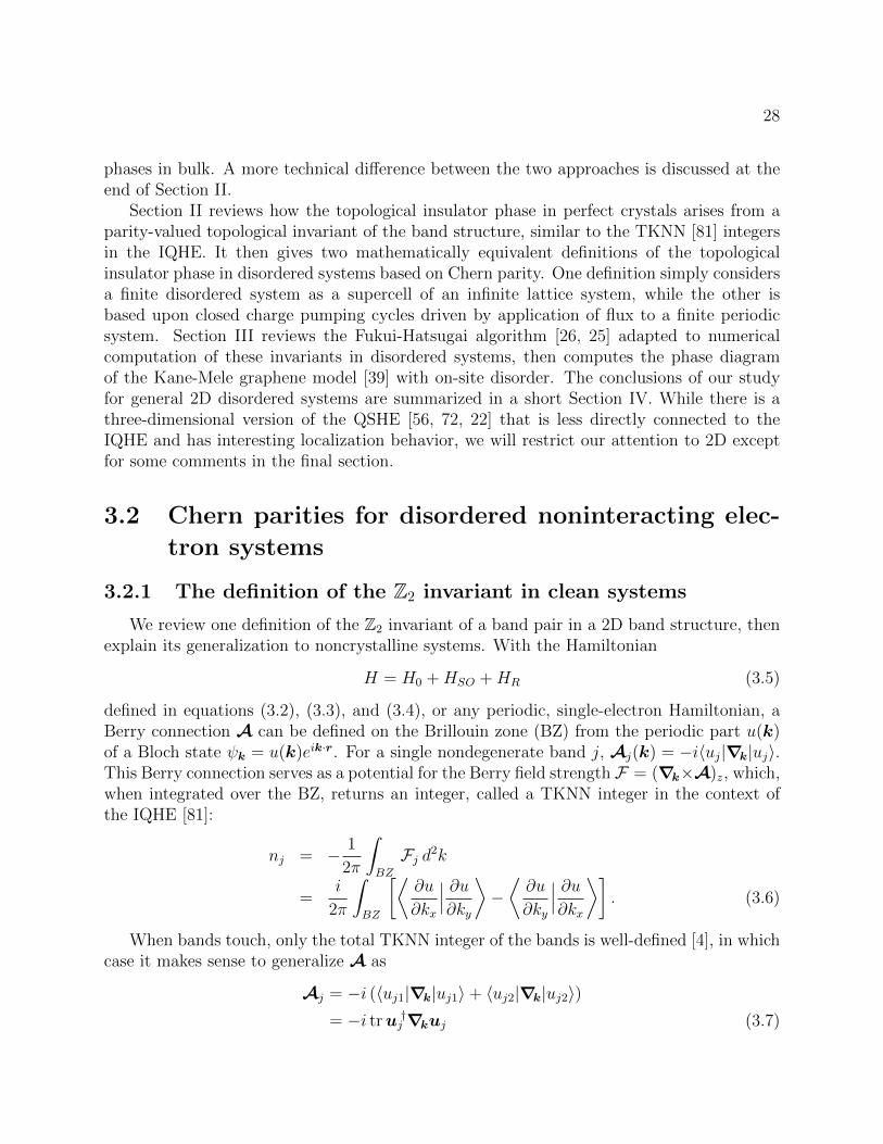
3.1 Graphene model of topological insulator . . . . . . . . . . . . . . . . . . . . 253.2 Effective Brillouin zone . . . . . . . . . . . . . . . . . . . . . . . . . . . . . . 303.3 Charge pumping for Chern parity . . . . . . . . . . . . . . . . . . . . . . . . 333.4 Schematic phase diagram with disorder . . . . . . . . . . . . . . . . . . . . . 343.5 Twist space . . . . . . . . . . . . . . . . . . . . . . . . . . . . . . . . . . . . 363.6 Distribution of Chern parities for band pairs . . . . . . . . . . . . . . . . . . 383.7 Metallic phase . . . . . . . . . . . . . . . . . . . . . . . . . . . . . . . . . . . 403.8 No metallic phase with added symmetry . . . . . . . . . . . . . . . . . . . . 413.9 Finite size scaling of crossover . . . . . . . . . . . . . . . . . . . . . . . . . . 423.10 Numerical phase diagram . . . . . . . . . . . . . . . . . . . . . . . . . . . . . 43

4.1 Magnetoelectric polarizability as a function of model parameter . . . . . . . 504.2 Surface Hall conductivity . . . . . . . . . . . . . . . . . . . . . . . . . . . . . 51

5.1 Geometry of polarization in a magnetic field . . . . . . . . . . . . . . . . . . 615.2 Schematic band structure that leads to vanishing αG . . . . . . . . . . . . . 635.3 Tetrahedral tight-binding model . . . . . . . . . . . . . . . . . . . . . . . . . 655.4 Currents induced by a magnetic field . . . . . . . . . . . . . . . . . . . . . . 67

iv

List of Tables

A.1 Comparison of Berry-phase theories of polarization and magnetoelectric po-larizability. . . . . . . . . . . . . . . . . . . . . . . . . . . . . . . . . . . . . . 88

v

Acknowledgments

This thesis is primarily a record of some of the research I have worked on during my timeas a graduate student at UC Berkeley, and much of the credit for the results presented, andfor whatever success I have had, must rest with others.

Most significantly, Professor Joel Moore has suggested the problems I have studied andgiven me the background I needed as well as the methods, and sometimes even the computercode. Even more importantly, he has helped me to work through my shortcomings as aresearcher when appropriate, and also has tried to show me when to abandon an unproductiveline of work.

Besides Joel, my collaborators David Vanderbilt and Ari Turner deserve much of thecredit for the results presented in this dissertation. Indeed, Ari is largely responsible forpushing me to actually work on the fully quantum treatment of the orbital magnetoelectricresponse, and he was the one to show that a derivation from density-matrix perturbationtheory is possible. In addition to his concrete contributions to this research, David’s alter-native perspective on the interesting and important features of condensed matter systemswas uniformly enlightening.

I also want to thank Andrei Malashevich and especially Ivo Souza for many discussionsabout magnetoelectric effects and the derivation of the response function. Although weeventually wrote two separate papers on the topic rather than one gigantic paper, they werestill instrumental to the progress of the research. Andrei, one of the world’s two expertsin the numerical computation of orbital magnetoelectric responses, was gracious enough tocompute the responses in a model I cooked up that was too challenging for my numericalabilities.

Ivo deserves further thanks, along with Roger Mong and Marcel Franz, for bringing to myattention numerical errors in the published version of the results presented here in Chapter 4.

Thanks to Hal Haggard for fielding my random questions about various topics in physicsand mathematics, and for giving a careful reading to a part of this thesis. Thanks are alsodue to Alex Selem, with whom I had a couple of productive discussions that ultimately ledto the model Hamiltonian presented in Chapter 4.

Finally, I need to thank Joel and Professors Joe Orenstein, Yuri Suzuki, and AshvinVishwanath for their tolerance of my weak performance during my qualifying exam, andtheir belief that I had potential in spite of that. Thanks also to Professor Suzuki for helpfulcomments on the first chapter of this manuscript.

Some of the work presented here has been published by the American Physical Society.The contents of Chapter 3 appeared in Phys. Rev. B 76, 165307 (2007). The contents ofChapter 4 appeared in Phys. Rev. Lett. 102, 146805 (2009). The contents of Chapter 5 havejust appeared in Phys. Rev. B 81, 205104 (2010).

Thanks to the Army Research Office for funding part of my graduate education througha National Defense Science and Engineering Graduate Fellowship, and thanks also to theWestern Institute for Nanoelectronics for my last two years of research support. The com-putations in Chapter 3 were done on the SUR cluster donated by IBM.

1

Chapter 1

Background and overview

One of the major driving motivations in condensed matter physics is the search fornew phases of matter, that is, new materials with novel properties. Sometimes these newproperties lead directly to important technologies. Sometimes they “merely” illuminatepreviously obscure possibilities in the structure of the laws that govern the natural world.Sometimes they even manage to do both.

The work I will present in the following chapters grows out of the recent theoreticaland, increasingly, experimental development of a new class of materials termed “topologicalinsulators”. In some sense the name is misleading, since there have been systems deservingof the name for nearly thirty years, and in principle the new discoveries form only a subsetof all topological insulators. In particular, the new materials are nonmagnetic topologicalband insulators.

In the rest of this chapter, I want to introduce the key features of topological insulators,or at least those that are not covered in greater depth later on. Before doing so, it seemsworthwhile to start at a relatively basic level and review the notion of a band insulator (andthe contrasting notion of a metal) and that of a topological property.

1.1 Band theory of solids

In middle school, I was taught that materials are divided into two classes: conductors(metals) that carry electricity, and insulators that don’t. The work I will be presenting dealswith new kinds of insulators (and a little about metals), so I want to review a simple pictureof how insulating or conducting behavior comes about, to serve as a reference point thathighlights why the new materials are interesting.

The electronic spectrum of an atom is divided into two pieces, the bound states andthe “scattering” (unbound) states. The bound state spectrum of an atom consists of levelslabeled by n, the “principal quantum number”, which are separated by energy gaps. Thisdiscrete energy spectrum is a consequence of, or is at least related to, the localized nature ofthe electron wave functions. An atom also has a “scattering” spectrum, consisting of those

2

states that are not bound to the atom. Qualitatively, these are extended free-particle statesthat get modified slightly by the presence of the nucleus.

Is the spectrum of a solid more like the bound-state state spectrum of an atom or thecontinuum? Are the states localized or extended? On the one hand, a solid is frequentlyconceived as being built of atoms, which suggests the former; on the other hand, thinkingabout nuclei and electrons rather than atoms, the (relatively) tightly packed nuclei mightjust provide an environment in which the electrons can run around.

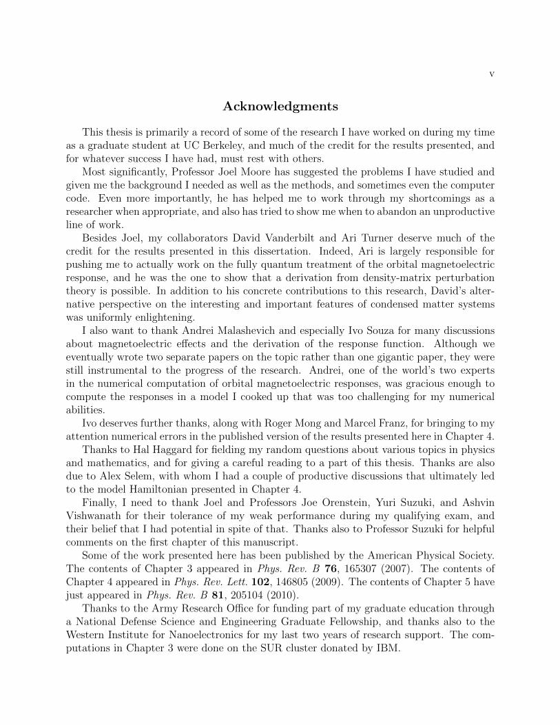
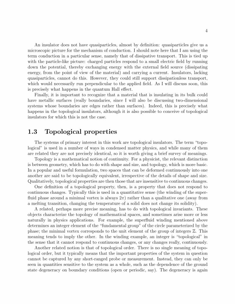
The simplest picture starts from atoms. Consider a bunch of isolated atoms, all of thesame species for true simplicity. Because electrons are fermions and therefore obey the Pauliexclusion principle (each state can only accommodate one electron at a time), they fill up thelowest few states of the discrete atomic spectrum (at zero temperature, which is the situationfor all the work I will present here). In this situation, the electrons are localized, that is, notfree to run around in the system. In some sense this is like the vacuum itself, which also hasno particles. If we imagine bringing the atoms closer together, the small overlap in the wavefunctions of two atoms will allow the electrons to tunnel back and forth. This also producesan energy splitting, but the splitting is much smaller than the atomic energy spacing. Inthis picture, each atomic level broadens into an energy “band”, see Figure 1.1.

E

a

Figure 1.1: Energy bands connect continuously to the limit of separated atoms, where theatomic spacing a tends to ∞. At finite separation the hybrid orbitals develop a spread inenergy (“bandwidth”). The dashed line indicates the physical spacing in a material.

Now we can try to answer the question, Does the material conduct or not?; Are the elec-trons free or bound? Each band n (generalizing the principal quantum number) is essentiallya continuum of states, in which a traveling wave packet can exist. However, if a band isfilled, there are no states available from which to assemble such a packet. An unfilled bandshould be conducting, while a filled band will be insulating. In this way, the band theory ofsolids gives a simple way to understand metals and insulators; metals have partially filled

3

bands, while insulators have filled bands.Of course, this simple picture cannot account for all metallic and insulating materials.

Most importantly, it assumes that the electrons do not interact with each other. Sinceelectrons repel, a situation can arise in which electrons localize (stop conducting) so as tominimize the repulsive energy, even though the band theory would predict metallic behavior.

The topological insulators that are the primary subject of the work I will present areband insulators, but with a difference. In particular, assuming that no magnetism develops(technically, that time reversal symmetry is unbroken), the band gap will have to close upontrying to take the (isolated) atomic limit of a topological insulator. When the band gapcloses, the system becomes a metal, and therefore fundamentally different from an insulator(at least in its transport properties). In this sense, the topological insulator is a distinctphase of matter from the “ordinary” or “trivial” insulator. It should be noted, however,that time-reversal breaking allows the possibility of an atomic (or at least molecular) limit.In this sense, the phase transition is more real than the phases themselves, rather like thetransition between liquid water and water vapor.

1.2 Insulators, metals, and quasiparticles

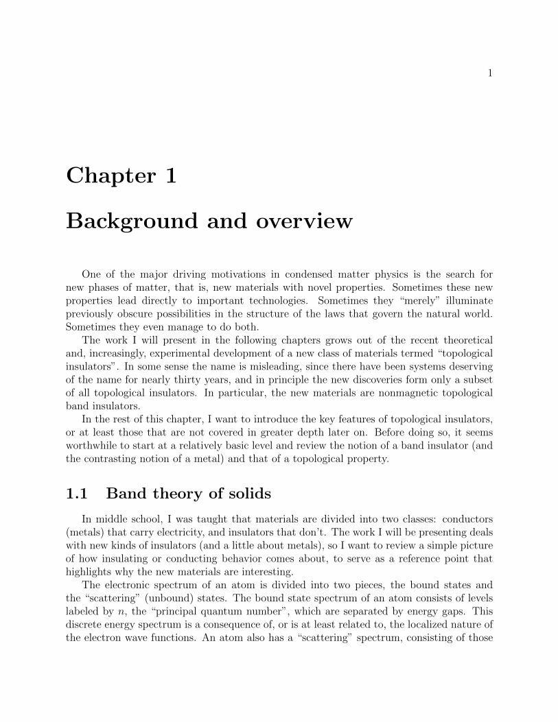
In the case of metals, I said above that partially filled bands can support traveling wavepackets. In such a situation, the dispersion relation between energy and momentum is crucialfor understanding the wave packet motion. Indeed, it is typically more intuitive to thinkof particles of definite momentum and energy when possible, even though the associatedwave functions will not be normalizable in an infinite system. Now, the atomic cores in asolid exert electrostatic forces on the electrons and break conservation of momentum, but ametal will still have sharply defined excitations with good energy and momentum quantumnumbers; this is Landau’s notion of the “quasiparticle”, essentially an electron but with adifferent dispersion relation (and also a finite lifetime).

k

Figure 1.2: A generic quasiparticle dispersion in a metal. The dashed line indicates thechemical potential, below which all states are filled at zero temperature.

4

An insulator does not have quasiparticles, almost by definition: quasiparticles give us amicroscopic picture for the mechanism of conduction. I should note here that I am using theterm conduction in a particular sense, namely that of dissipative transport. This is tied upwith the particle-like picture: charged particles respond to a small electric field by runningdown the potential, thereby exchanging energy with the external field source (dissipatingenergy, from the point of view of the material) and carrying a current. Insulators, lackingquasiparticles, cannot do this. However, they could still support dissipationless transport,which would necessarily run perpendicular to the applied field. As I will discuss soon, thisis precisely what happens in the quantum Hall effect.

Finally, it is important to recognize that a material that is insulating in its bulk couldhave metallic surfaces (really boundaries, since I will also be discussing two-dimensionalsystems whose boundaries are edges rather than surfaces). Indeed, this is precisely whathappens in the topological insulators, although it is also possible to conceive of topologicalinsulators for which this is not the case.

1.3 Topological properties

The systems of primary interest in this work are topological insulators. The term “topo-logical” is used in a number of ways in condensed matter physics, and while many of themare related they are not precisely identical, so it is worth giving a brief survey of meanings.

Topology is a mathematical notion of continuity. For a physicist, the relevant distinctionis between geometry, which has to do with shape and size, and topology, which is more basic.In a popular and useful formulation, two spaces that can be deformed continuously into oneanother are said to be topologically equivalent, irrespective of the details of shape and size.Qualitatively, topological properties are then those that are insensitive to continuous changes.

One definition of a topological property, then, is a property that does not respond tocontinuous changes. Typically this is used in a quantitative sense (the winding of the super-fluid phase around a minimal vortex is always 2π) rather than a qualitative one (away froma melting transition, changing the temperature of a solid does not change its solidity).

A related, perhaps more precise meaning, has to do with topological invariants. Theseobjects characterize the topology of mathematical spaces, and sometimes arise more or lessnaturally in physics applications. For example, the superfluid winding mentioned abovedetermines an integer element of the “fundamental group” of the circle parameterized by thephase; the minimal vortex corresponds to the unit element of the group of integers Z. Thismeaning tends to imply the other. In the winding example, an integer is “topological” inthe sense that it cannot respond to continuous changes, or any changes really, continuously.

Another related notion is that of topological order. There is no single meaning of topo-logical order, but it typically means that the important properties of the system in questioncannot be captured by any short-ranged probe or measurement. Instead, they can only beseen in quantities sensitive to the system as a whole, such as the dependence of the groundstate degeneracy on boundary conditions (open or periodic, say). The degeneracy is again

5

an integer, which makes this topological in the above sense. This example also illustratesthe sort of drastic change, like cutting open a boundary, needed to change a topologicalproperty.

The topological insulators that are the subject of this dissertation fit most naturally intothe definition in terms of topological invariants, but all the characterizations above work togreater or lesser degree.

I will review some of the known properties of topological insulators in this introductionand in the subsequent chapters. For more complete coverage, I refer the reader to a fewgood, general reviews of the subject that have appeared recently. Moore [58] and Qi andZhang [68] have written reasonably qualitative introductions for a general audience, whileHasan and Kane [31] have written a detailed review of the theoretical and experimental stateof the art.

1.4 The quantum Hall effect

The prototypical topological systems are those that exhibit the quantum Hall effect.The effect was originally seen in the two dimensional gas of electrons that forms at theboundary between GaAs and AlGaAs, and has now also been seen in graphene, the trulytwo dimensional crystalline form of carbon. In sufficiently clean samples, at low enoughtemperatures,1 and in a strong enough magnetic field perpendicular to the plane of theelectrons, it is found that the (longitudinal) conductance σxx vanishes, while the (transverse)Hall conductance σH = σxy takes values that are integer multiples, or simple fractions, of thenatural unit of conductivity e2/h, where e is the electron charge and h is Planck’s constant.2

Since the Hall conductance takes its values in a discrete set under these conditions, it qualifiesas a topological property by the above definitions.

The crucial prerequisites for quantum Hall physics are the dimensionality (two dimen-sions, specifically) and the breaking of time reversal symmetry T supplied by the strongmagnetic field. To show this explicitly, Haldane constructed a theoretical band insulatorthat provides a minimal model of the integer effect [29]; he considered spinless electronshopping on a honeycomb lattice, with broken time reversal symmetry but with vanishingaverage magnetic field, and showed that the Hall conductance could be 0 or ±1 (in unitsof e2/h), depending on parameters.3 It is quite straightforward to see that such an effectmust break T : in the equation Jx = σHE

y, the current J breaks T (run time backward andthe current will flow backward, not stay the same) but the electric field E does not, so thematerial property σH must capture a symmetry breaking in the material.

Note that something quite mysterious must be going on here. These systems are bandinsulators (the integer states, anyway), whose spectrum includes only “inert” filled bands.

1Room temperature in graphene.2In two dimensions, conductance has the units of conductivity.3This sort of thing could also occur in three dimensions, but essentially only as a collection of two

dimensional layers.

6

Apparently these bands are not so inert after all. I noted earlier that this sort of thing couldarise in principle: since the Hall current is perpendicular to the applied field, no momentumis transferred to the electrons and no energy dissipated. It may be hard to visualize themechanism of conduction, since there are no states from which to build wave packets, butat least this phenomenon is consistent with energy conservation.

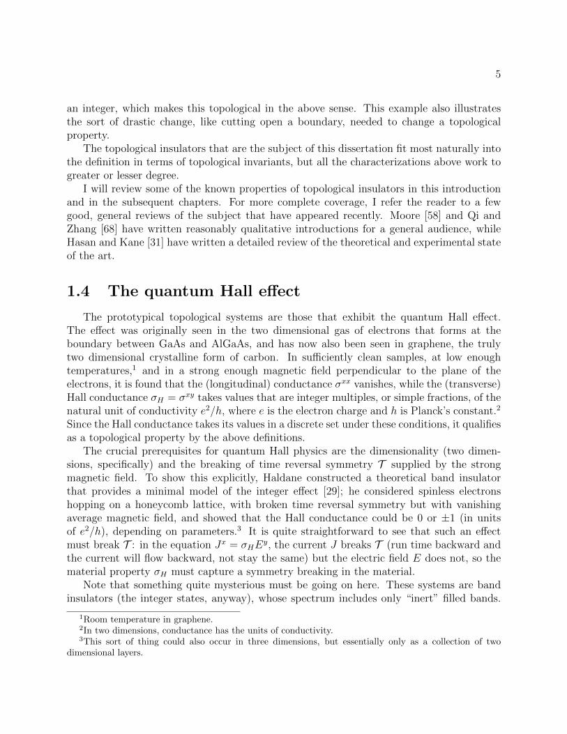
It turns out to be enlightening to consider the difference between open and periodicboundary conditions. The statement that the Haldane model is a bulk insulator only refersto the bulk of the system and not its boundaries. The standard theoretical device foreliminating the effect of boundaries involves using periodic boundary conditions, but thiscan mask effects that become apparent with open boundaries, as in cases of topologicalorder. In the present case, it turns out that the edges must be metallic; each edge carriesan integer number of “edge modes” (the same integer as the conductance) that are “chiral”(propagate in one direction only) and so capture the broken time reversal symmetry [46, 30].In a sample with one edge (disk topology), one can then take the view that all the physicsoccurs at the edge, with the bulk completely inert. This goes by the name “bulk-boundarycorrespondence”.

e

quantumHall fluid

Figure 1.3: The edge of a quantum Hall system carries an electronic mode that is chiral,i.e., that propagates in only one direction.

1.5 Topological insulators with time reversal symme-

try

It was thought that there could be no analogous topologically nontrivial band insulatorsthat preserve T . However, a thought experiment by Kane and Mele [39, 40] shows thatthere should be a two dimensional case. The construction is quite simple. First, supposethere are two kinds of electron (say, in two layers), and the T breaking for one is equal andopposite to that for the other. Then there is no overall T breaking, and no net quantum Hall

7

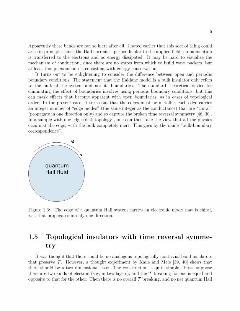
effect, but there are still chiral edge modes, running in opposite directions. Now supposethat the two kinds of electron are the two values for some component of spin. Spin, as anangular momentum, breaks T , but spin up is precisely the time reverse of spin down, sothe two together still preserve T . In particular, the edge mode for one species of spin is thetime reverse of the other. It is not too difficult to show that no T -invariant perturbationto the Hamiltonian can mix these states (i.e., no T -invariant operator has a nonzero matrixelement between these states), and so no T -invariant mixing of the two species in the bulkof the system will affect the existence of the edge states. The crucial fact is that T 2 = −1for half-odd spins (spin-1/2 in the case of electrons).

Figure 1.4: The edge of a topological insulator in two dimensions carries a counterpropa-gating, “helical” pair of electronic modes.

This insensitivity points to the presence of a bulk topological invariant, although it isnot given simply by a conductivity or other response function. In this way, the T -invarianttopological insulator is a more subtle system than the integer quantum Hall insulator, andprobes sensitive to the edge states are needed to verify the presence of the topological state.This state has been reported in HgCdTe/CdTe/HgCdTe wells; the experiment looked forsignatures of one-dimensional metallic conduction, characteristic of edge modes [8, 44].

Another difference from the quantum Hall case is the existence of an intrinsically three-dimensional T -invariant topological insulator, not just layered versions of the two-dimensionalone just discussed [22, 56, 72]. This system, by contrast, does exhibit a topological bulkresponse property, in this case the zero-field magnetoelectric polarizability. A number ofmaterials, including BiSb alloy, Bi2Se3, and Bi2Te3 [37, 85, 14], have been verified to be inthis class, although the probes have again been sensitive to the surface states and not tothe bulk response function. The surface states of the 3d topological insulator should againspan the bulk gap so that the surface is metallic at any chemical potential. In caricature,the surface states look like a cone, which is typically referred to as a “Dirac cone”, because aconical 2d dispersion relation can be described by a massless Dirac equation. In particular,

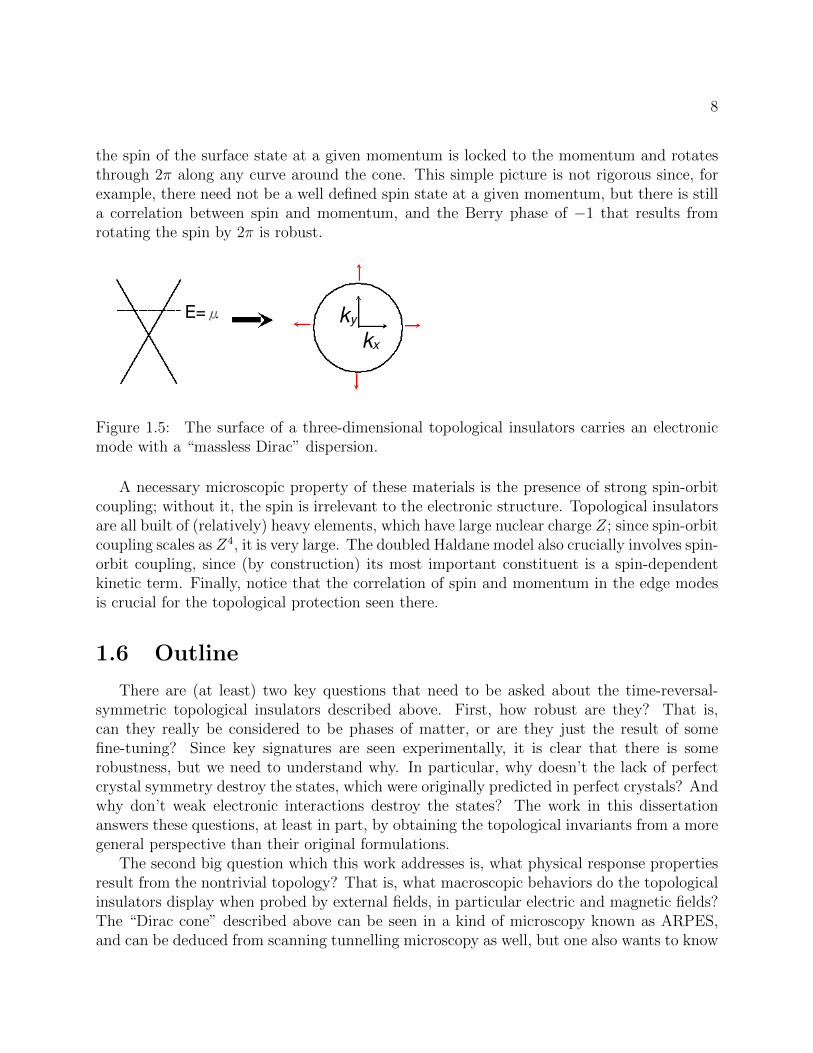
8

the spin of the surface state at a given momentum is locked to the momentum and rotatesthrough 2π along any curve around the cone. This simple picture is not rigorous since, forexample, there need not be a well defined spin state at a given momentum, but there is stilla correlation between spin and momentum, and the Berry phase of −1 that results fromrotating the spin by 2π is robust.

Figure 1.5: The surface of a three-dimensional topological insulators carries an electronicmode with a “massless Dirac” dispersion.

A necessary microscopic property of these materials is the presence of strong spin-orbitcoupling; without it, the spin is irrelevant to the electronic structure. Topological insulatorsare all built of (relatively) heavy elements, which have large nuclear charge Z; since spin-orbitcoupling scales as Z4, it is very large. The doubled Haldane model also crucially involves spin-orbit coupling, since (by construction) its most important constituent is a spin-dependentkinetic term. Finally, notice that the correlation of spin and momentum in the edge modesis crucial for the topological protection seen there.

1.6 Outline

There are (at least) two key questions that need to be asked about the time-reversal-symmetric topological insulators described above. First, how robust are they? That is,can they really be considered to be phases of matter, or are they just the result of somefine-tuning? Since key signatures are seen experimentally, it is clear that there is somerobustness, but we need to understand why. In particular, why doesn’t the lack of perfectcrystal symmetry destroy the states, which were originally predicted in perfect crystals? Andwhy don’t weak electronic interactions destroy the states? The work in this dissertationanswers these questions, at least in part, by obtaining the topological invariants from a moregeneral perspective than their original formulations.

The second big question which this work addresses is, what physical response propertiesresult from the nontrivial topology? That is, what macroscopic behaviors do the topologicalinsulators display when probed by external fields, in particular electric and magnetic fields?The “Dirac cone” described above can be seen in a kind of microscopy known as ARPES,and can be deduced from scanning tunnelling microscopy as well, but one also wants to know

9

the macroscopic characteristics as well; this both connects to well-established experimentalparadigms in condensed matter physics, and is important if these materials are ever to findpractical, technological application. The chapters to follow give partial answers to this crucialquestion as well.

The remainder of this chapter will introduce in more detail the specific topics to becovered in this dissertation. Chapter 2 reviews some important technical tools and results;in particular, I discuss Bloch’s theorem for periodic potentials and the derivation of adiabaticcharge transport (the “Kubo formula”). Both these results are crucial for understanding theHall conductivity as a bulk topological invariant in the integer quantum Hall regime. I havechosen to present the Kubo formula in a many-body formulation, which hopefully providesconceptual clarity, as well as in a relatively idiosyncratic single-particle formulation thatexplicitly allows degenerate energy levels and that relies on Bloch’s theorem (and henceperiodicity) minimally.

The original definitions of the topological invariant characterizing the two-dimensionaltopological insulator rely on the strict periodicity of the material. Chapter 3 reviews oneof the more practically useful formulations of the topological invariant and generalizes it todisordered systems. This generalization is important in its own right, and it provides a wayto make contact with an old result on 2d systems, namely, that a disordered 2d materialwith strong spin-orbit coupling should be metallic. The bulk topological invariant does notdirectly detect this metallic behavior; instead, it reveals the presence of a transition betweendistinct insulating phases. The transition between integer quantum Hall states remains sharpin the presence of disorder, whereas disorder turns out to broaden the transition between thetime-reversal invariant topological insulator and the ordinary insulator. This can be takenas confirmation that a noninsulating, hence metallic, phase intervenes.

Chapters 4 and 5 treat three-dimensional band insulators. In contrast to the two-dimensional case studied in Chapter 3, the three-dimensional topological invariant (or oneformulation of it, anyhow) gives a quantized magnetoelectric response [67], very analogousto the quantized Hall conductivity in integer quantum Hall systems. The magnetoelectricresponse is the response of the electronic polarization P to an applied magnetic field B,or alternatively the response of the magnetization M to an applied electric field E. In theabsence of dissipation, as in an insulator (so long as the field frequency is smaller than thegap to excitations), these two responses are equal.

The most important result in chapter 4 is that, like the quantum Hall case, this quantizedresponse is (at least in principle) robust to disorder and interactions, and therefore servesto define topological insulators absolutely generally. This result follows directly from now-standard results on the electronic contribution to the polarization of bulk systems, togetherwith some simple geometry. I will review the modern theory of polarization in Chapter2 as part of the technical introduction, to serve as background for this result. Chapter4 also uses a nice result from the modern treatment of semiclassical band dynamics [87]to give a simple derivation of the expression for the invariant in the noninteracting case,first derived by evaluating a Feynman diagram in a 4+1 dimensional field theory and thendimensionally reducing down [67]. Finally, in Chapter 4 I show that it is possible to evaluate

10

the topological invariant in a number of ways, both directly from the derived expression andmore physically as the polarization response to an applied magnetic field or as the surfaceHall conductivity of a slab. To make these results more general, I have also extended the firstmodel Hamiltonian of a 3d topological insulator [22], breaking time reversal symmetry byadding a coupling to an antiferromagnetic parameter, which allows a smooth interpolation(or “adiabatic continuation”) between the topological and trivial phases. This interpolationcan almost be seen as an extra dimension in the problem, making contact at some level withthe original derivation of the response.

Chapter 5 revisits the general problem of the magnetoelectric response, without muchspecific reference to topological insulators, and derives the full orbital contribution to theDC linear magnetoelectric response of a crystalline band insulator in the “frozen lattice”limit.4 From the perspective of computing the properties of real materials, this can be seenas a very limited result; however, it proves to be the most technically challenging part of thelinear response problem, and in fact it is already known how to compute all other contribu-tions. Furthermore, the predicted value of this orbital coupling for topological insulators iscomparable to measured values of the full magnetoelectric effect in a benchmark material,Cr2O3 [32], so the formulae presented here may prove useful as the interest in topologicalinsulators and related compounds continues to increase. Notably, the fully quantum me-chanical derivation of Chapter 5 is able to compute explicitly terms that the semiclassicalmethod of Chapter 4 cannot. In particular, Chapter 5 provides a solution to the problem ofcomputing the response to a uniform magnetic field in a crystal, and it is my hope that themethods developed here may prove more generally useful for such problems.

4This work was done concurrently with Ivo Souza and Andrei Malashevich at UC Berkeley, who gave adifferent derivation of the same results and who have published them in a concurrent paper [51].

11

Chapter 2

Technical review and introduction

2.1 Insulators

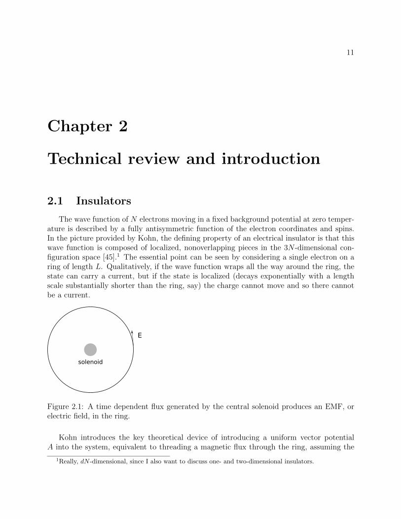
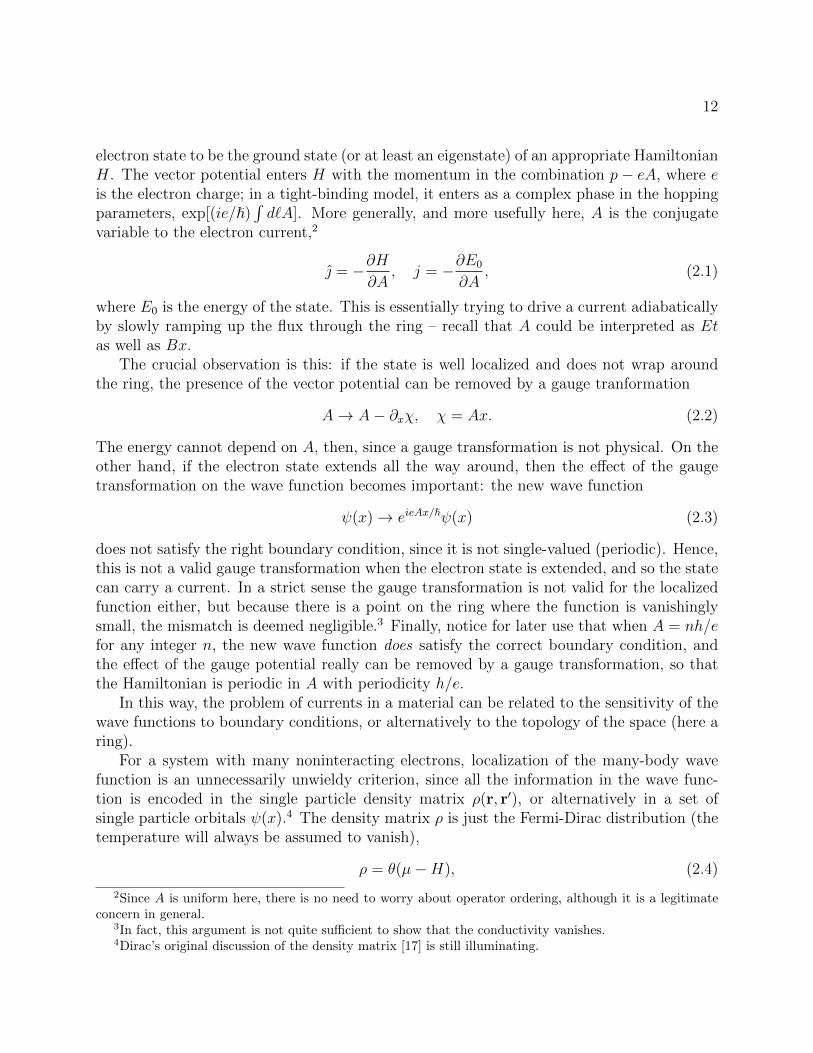
The wave function of N electrons moving in a fixed background potential at zero temper-ature is described by a fully antisymmetric function of the electron coordinates and spins.In the picture provided by Kohn, the defining property of an electrical insulator is that thiswave function is composed of localized, nonoverlapping pieces in the 3N -dimensional con-figuration space [45].1 The essential point can be seen by considering a single electron on aring of length L. Qualitatively, if the wave function wraps all the way around the ring, thestate can carry a current, but if the state is localized (decays exponentially with a lengthscale substantially shorter than the ring, say) the charge cannot move and so there cannotbe a current.

solenoid

E

Figure 2.1: A time dependent flux generated by the central solenoid produces an EMF, orelectric field, in the ring.

Kohn introduces the key theoretical device of introducing a uniform vector potentialA into the system, equivalent to threading a magnetic flux through the ring, assuming the

1Really, dN -dimensional, since I also want to discuss one- and two-dimensional insulators.

12

electron state to be the ground state (or at least an eigenstate) of an appropriate HamiltonianH. The vector potential enters H with the momentum in the combination p− eA, where eis the electron charge; in a tight-binding model, it enters as a complex phase in the hoppingparameters, exp[(ie/)

∫d`A]. More generally, and more usefully here, A is the conjugate

variable to the electron current,2

= −∂H∂A

, j = −∂E0

∂A, (2.1)

where E0 is the energy of the state. This is essentially trying to drive a current adiabaticallyby slowly ramping up the flux through the ring – recall that A could be interpreted as Etas well as Bx.

The crucial observation is this: if the state is well localized and does not wrap aroundthe ring, the presence of the vector potential can be removed by a gauge tranformation

A→ A− ∂xχ, χ = Ax. (2.2)

The energy cannot depend on A, then, since a gauge transformation is not physical. On theother hand, if the electron state extends all the way around, then the effect of the gaugetransformation on the wave function becomes important: the new wave function

ψ(x)→ eieAx/ψ(x) (2.3)

does not satisfy the right boundary condition, since it is not single-valued (periodic). Hence,this is not a valid gauge transformation when the electron state is extended, and so the statecan carry a current. In a strict sense the gauge transformation is not valid for the localizedfunction either, but because there is a point on the ring where the function is vanishinglysmall, the mismatch is deemed negligible.3 Finally, notice for later use that when A = nh/efor any integer n, the new wave function does satisfy the correct boundary condition, andthe effect of the gauge potential really can be removed by a gauge transformation, so thatthe Hamiltonian is periodic in A with periodicity h/e.

In this way, the problem of currents in a material can be related to the sensitivity of thewave functions to boundary conditions, or alternatively to the topology of the space (here aring).

For a system with many noninteracting electrons, localization of the many-body wavefunction is an unnecessarily unwieldy criterion, since all the information in the wave func-tion is encoded in the single particle density matrix ρ(r, r′), or alternatively in a set ofsingle particle orbitals ψ(x).4 The density matrix ρ is just the Fermi-Dirac distribution (thetemperature will always be assumed to vanish),

ρ = θ(µ−H), (2.4)

2Since A is uniform here, there is no need to worry about operator ordering, although it is a legitimateconcern in general.

3In fact, this argument is not quite sufficient to show that the conductivity vanishes.4Dirac’s original discussion of the density matrix [17] is still illuminating.

13

where θ is the Heaviside step function and µ is a chemical potential. The two crucialproperties of this operator for what follows are

• ρ2 = ρ (idempotency): ρ is a projection operator onto the filled single-electron states.

• [H, ρ] = 0: ρ is an eigenoperator of the Hamiltonian.

It is important to realize that all the occupied electronic levels, that is, those with energy lessthan µ, are degenerate when considered as eigenstates of ρ, and similarly for the unoccupiedlevels; the former have eigenvalue 1, the latter 0. Physical quantities should not dependon the eigenstates and energies of H individually, but only as a group. This is effectivelyanother kind of “gauge invariance”, a redundancy introduced by using the (otherwise moreconvenient) description of the many-electron wave function in terms of the single particledensity matrix.

2.2 Adiabatic conduction, charge pumping, and geom-

etry

It will prove useful to have a more quantitative account of an adiabatically driven current.I will provide two derivations, one in terms of the many electron wave function and one interms of the one electron density matrix. The formula generated is called a Kubo formula,5

although zero-temperature derivations of the Kubo formula for conductivity typically assumean electric field that oscillates at a finite frequency. There is another useful formalism,“semiclassical dynamics”, which I will not review here but which is the basis for the mainderivation in Chapter 4. A comprehensive treatment from a modern viewpoint is given byXiao, Chang, and Niu [86]. That review also covers much of the material in this section andthe next, but it seems worthwhile to include it here anyway.

The adiabatic approximation to the ground state of a Hamiltonian H(λ(t)) that variesslowly is just the instantaneous ground state ψ0,

ψ(t) ≈ eiφ(t)ψ0(λ), H(λ)ψ0(λ) = E0(λ)ψ0(λ), H(λ) = H(0) + λOλ. (2.5)

The phase factor takes care of the usual dynamical evolution in a time-independent Hamilto-nian, as well as the arbitrariness inherent in identifying the ground states at different valuesof the parameter. However, this is not a satisfactory approximation here; it predicts thatthe current driven by an adiabatic change is just

〈ψ0(λ)|j|ψ0(λ)〉, (2.6)

which is just the current that would exist if the Hamiltonian were not varying. At the nextorder of approximation,

|ψ(t)〉 ≈ exp iφ(t)

[|ψ0(λ)〉+ iλ

∑m6=0

|ψm(λ)〉〈ψm(λ)|∂λψ0(λ)〉Em(λ)− E0(λ)

], (2.7)

5Or Kubo-Greenwood or even Kubo-Greenwood-Peierls

14

wherein it can be seen explicitly that the accuracy of the approximation is governed by thesize of the excitation gap E1 − E0 in addition to the rate of change λ.6 Then

〈Oλ′〉(t) = iλ∑m 6=0

〈ψ0(λ)|Oλ′|ψm(λ)〉〈ψm(λ)|∂λψ0(λ)〉Em(λ)− E0(λ)

+ c.c., (2.8)

assuming the zeroth order term vanishes. Now, a very useful relation follows directly fromthe definition of the instantaneous eigenstates,

H(λ)ψ0(λ) = E0(λ)ψ0(λ)⇒ 〈ψm(λ)|∂λψ0(λ)〉 =〈ψm(λ)|∂λH(λ)|ψ0(λ)〉

Em(λ)− E0(λ). (m 6= 0) (2.9)

This leads to two alternative formulations:

〈Oλ′〉(t) = iλ∑m6=0

〈ψ0|Oλ′ |ψm〉〈ψm|Oλ|ψ0〉 − c.c.

(Em − E0)2(2.10)

and〈Oλ′〉(t) = iλ [〈∂λ′ψ0|∂λψ0〉 − 〈∂λψ0|∂λ′ψ0〉] . (2.11)

There is really a factor 1− |ψ0〉〈ψ0| in the latter inner products, but it drops out of the realpart. In the case of currents, the conjugate variables λ, λ′ are given by components of thevector potential,

〈ji〉(t) = iEj[〈∂Ai

ψ0|∂Ajψ0〉 − 〈∂Aj

ψ0|∂Aiψ0〉], (2.12)

that is,σij = i

[〈∂Ai

ψ0|∂Ajψ0〉 − 〈∂Aj

ψ0|∂Aiψ0〉]. (2.13)

Notice that the diagonal conductivity, indeed the symmetric part, vanishes automati-cally: the adiabatic approximation applies precisely when energy is not being pumped intothe system (excitations are gapped), and so there cannot be a longitudinal current (whichdissipates energy).

The derived expression for the conductivity has a geometric interpretation. Wave func-tions Ψ live in a complex projective space, which we usually imagine to be embedded in aHilbert space. A natural metric exists to measure distances and angles, acting on tangentvectors to the Hilbert space δΨ. This is called the Fubini-Study metric, and takes the form

g(δΨ1, δΨ1)(Ψ) = 〈δΨ1|(1− |Ψ〉〈Ψ|)|δΨ2〉, (2.14)

where Ψ is again a point in the complex projective space, while the inner product is theHilbert space inner product [94]. The projector 1−|Ψ〉〈Ψ| appears because any component ofδΨ parallel to Ψ does not point to a state physically different from Ψ. Now, if Ψ = ψ0(λ, λ

′),δΨ1 = ∂λψ0δλ, and δΨ2 = ∂λ′ψ0δλ

′, this becomes

gλλ′δλδλ′ = 〈∂λψ0|(1− |ψ0〉〈ψ0|)|∂λ′ψ0〉δλδλ′, (2.15)

6For an immensely detailed derivation of this old result, see [16].

15

and soσij = −2 Im

(gAiAj

). (2.16)

A more popular geometric interpretation is in terms of a curvature instead of a metric.In this case we write

fλλ′ = 〈∂λψ0|∂λ′ψ0〉 − 〈∂λ′ψ0|∂λψ0〉= ∂λ〈ψ0|∂λ′ψ0〉 − ∂λ′〈ψ0|∂λψ0〉= ∂λaλ′ − ∂λ′aλ, aλ ≡ 〈ψ0|∂λψ0〉, (2.17)

where aλ is called the Berry connection and fλλ′ the Berry curvature. This a really isthe connection of the fiber bundle created by projecting the trivial bundle λ × H, with λthe parameter space (λ, λ′) and H the Hilbert space, onto the ground-state subspace with|ψ0〉〈ψ0|, and f is the corresponding curvature. These definitions make a and f imaginary, ormore generally anti-Hermitian; later on, it will sometimes be convenient to use a Hermitiandefinition, A = ia and F = if .

The connection and curvature are named after Berry, who explored the effects of thisadiabatic geometric structure [9]. In particular, he noticed that after an adiabatic variationof parameters that forms a closed loop in λ, the true ground state wave function picks up aphase determined solely by a (or f) and quite independent of the usual factor

∫E0(t)dt/.

Indeed, it is possible to interpret both the Aharonov-Bohm effect and the nontrivial behaviorof a spin-1/2 under a 2π rotation as Berry phases.

Thouless [79] pointed out that such an effect can occur with a one-parameter adiabaticvariation if the Hamiltonian is periodic in the parameter. In particular, consider the insulatorHamiltonian on a ring, as discussed briefly earlier. Then the parameter λ might be theposition of a potential well that could be dragged slowly around the ring, for example. Thecurrent driven by any such variation that brings the Hamiltonian back to its original stateis, from before,

j = iλ[∂λaA − ∂Aaλ]. (2.18)

The total charge that flows will be given by

∆Q = ie

2π

∫ 1

0

dλ

∫ h/e

0

dA [∂λaA − ∂Aaλ], (2.19)

where the periodicity of the Hamiltonian in λ is assumed to be 1 and the periodicity in Ais h/e as noted earlier. The average over A is an admittedly strange thing to do, but sincethe system is assumed to be an insulator, Kohn’s criterion allows it.

The integral can be argued to be quantized in units of 2πi. The essence of the argumentrequires seeing the relation between the connection a and the phase of the instantaneousground state wave function ψ0. In particular, changes in phase are intimately tied to changesin the former,

ψ0 → eiχ(A,λ)ψ0 ⇒ aλ → aλ + i∂λχ, (2.20)

16

for example. Using Stokes’ theorem, the charge can be expressed as the line integral of the“vector potential” a around the boundary of the integration region, which by the last relationis tied to the winding of the phase around that boundary. If ψ0 is to be single-valued as afunction of parameters, this winding must be an integer multiple of 2π.

This argument means that ∆Q = ne for some integer n, that is, that adiabatic chargetransport, or pumping, is quantized in units of the fundamental charge. It is therefore ourfirst example of a topological quantity characterizing a physical process.

From a mathematical point of view, the charge pumped is given by the first Chern classof the ground state fiber bundle over the parameter space. As far as the Hamiltonian isconcerned, the parameter space (A, λ) is a torus T 2, since it is periodic in both parameters;so is the ground state projector |ψ0〉〈ψ0|, which generates the bundle in question. The Chernclass of a one-dimensional bundle over a compact two-dimensional manifold like T 2 is

C1 =i

2π

∫d2λ fλλ′ . (2.21)

The existence of such an integer can be deduced through a related construction. Theabove construction computes the “cohomology class” of the fiber bundle, but it is sometimeshelpful to think about the “homotopy” classes instead. In this approach, the goal is tofind the set of topologically distinct ways that a torus can be embedded into the space ofprojection matrices.

A simple example will serve to illustrate the connection. Consider a Hamiltonian

H(λ, λ′) = n · σ, n(λ, λ′) = (cosφ sin θ, sinφ sin θ, cos θ) (2.22)

where the spherical angles φ and θ are functions of the parameters. Because H2 = 1, it iseasy to see that the ground state projector is

P =1−H

2=

(sin2 θ

2− cos θ

2sin θ

2e−iφ

− cos θ2

sin θ2eiφ cos2 θ

2

)=(sin θ

2− cos θ

2e−iφ

)( sin θ2

− cos θ2eiφ

),

(2.23)and from the ground state spinor it is straightforward to compute7

fλλ′ = − i2

sin θ∂(θ, φ)

∂(λ, λ′). (2.24)

Naıvely this makes

C1 =1

4π

∫sin θdθdφ = 1, (2.25)

but this is not quite right. For example, ∂(θ, φ)/∂(λ, λ′) can take both positive and negativevalues, but the simple result given assumed that it was always positive. More importantly,

7For the computation, the differential forms notation simplifies things. In this notation, a = 〈ψ|d|ψ〉and f = da, where the differential operator is d =

∑i dλ

i∂λi and the differentials anticommute, dλidλj =−dλidλj .

17

the integral over λ, λ′ could cover the unit sphere θ, φ more than once, in which case therewould need to be an integral over the sphere for each covering. This means that C1 is just the“degree” of the map θ(λ, λ′), φ(λ, λ′). This is the idea of homotopy, which counts the waysthat one space can be mapped into another. The simple connection between cohomologyand homotopy indicated here does not hold in all cases, but it is important to recognize.

2.3 Electronic polarization (and magnetization)

Maybe it’s time to return to a more physical question for a while. In the charge pumpingexample, what if the parameter λ is not varied through its full range? In that case, thepumped charge need not be an integer. Suppose further that the ring-like system is composedof a finite sample of the insulating material of interest and a voltmeter that connects the twoends. Then the charge pumped is really the charge that flows through the zero-dimensionalsurface of the material. In the absence of the voltmeter, that charge would build up at theends; in an insulator, it cannot flow back away from the surface. By allowing it to flowthrough the voltmeter (which is really just a very large resistor, that measures the chargepumped through the known resistance) this experimental paradigm prevents a static electricfield due to the charge buildup from developing. In this way, one can compute an intrinsicdifference in the end charges between the initial and final states of the material.

In fact, this is the experimental procedure to determine the polarization of an insulator.This follows from the relation σ = P · n, where σ is the surface charge density (in this one-dimensional example, just the end charge), P is the polarization (dipole moment density),and n the surface normal. Two important points are worth noting: 1. This definition relieson the existence of a reference material with vanishing polarization, to which the substance ofinterest can be adiabatically deformed (at least theoretically); 2. Since the periodic variationcould in principle be run through an arbitrary number of times, there is an arbitrariness tothe polarization, with the discrete unit of arbitrariness e.

As a slight digression, the magnetization can be obtained by linear response methods aswell, and the result comes out more simply than in the case of polarization. The electromag-netic energy current density is given by the Poynting vector, S = E×H = E×B/µ0−E×M.Therefore, a computation of the response of the energy current Tr[ρHv], or at least a properlysymmetrized version thereof, to an applied electric field will yield the zero-field magnetiza-tion. The standard derivation of the orbital magnetization [78] starts from a finite systemand shows that the result can be written solely in terms of bulk quantities; this alternateapproach has the nice feature that it works entirely in the bulk.

2.4 Bloch’s theorem

From this point forward, almost all results will assume that electrons do not interact withanother except through a mean-field potential. Most results will also assume a crystallinesystem, in which case the lattice translation symmetry can be used to simplify the problem

18

of finding the ground state of the system, and thereby its response functions. The classicresult is Bloch’s theorem: the stationary states ψnk of a crystalline Hamiltonian satisfy thefollowing properties:

Hψnk = Enkψnk, ψnk(r + R) = eik·Rψnk(r). (2.26)

The quantum number k, called the wave number or the crystal momentum, takes valuesin any primitive unit cell of the reciprocal lattice, which is the set of vectors G such thatG ·R = 2πm for any integer m and any “direct” lattice vector R. It is also possible to allowk to take any value in the reciprocal lattice, in which case

ψnk+G = ψnk. (2.27)

I will use the name “the Brillouin zone” (BZ) for any useful choice of the primitive cell ofthe reciprocal lattice, even though that term refers to a particular choice of cell. Because ofthe periodicity in k, the BZ can be viewed as a torus, although one sometimes needs to becareful about this.

The second characteristic property of the wave functions means they can be decomposedinto a plane wave part, with wave number inside the BZ, and a periodic part u whose Fouriercomponents have wave numbers in G,

ψnk = eik·runk, unk(r + R) = unk(r). (2.28)

Notice that unk+G = e−iG·runk to be consistent with the periodicity of ψ, which is why itis good to be cautious about considering the BZ a torus. It can be useful to think of therelation between u and ψ as a unitary transformation; applying the same transformation tothe Hamiltonian allows us to define

Hk ≡ e−ik·rHeik·r, (2.29)

which I will call the Bloch Hamiltonian. The Bloch Hamiltonian is periodic in the spatialcoordinate r but, like the functions u it operates on, not in the reciprocal coordinate k.

The crucial object is the ground state density matrix,

ρ =∑n occ,k

|ψnk〉〈ψnk|, ρ(r, r′) =∑n occ,k

ψnk(r)ψ∗nk(r′). (2.30)

For future reference, note that∑

k = Ω∫BZ

d3k(2π)3

= NΩ0

∫BZ

d3k(2π)3

, where Ω is the volume ofthe crystal, with N unit cells of volume Ω0. It may be instructive to look at the differencebetween band metals and insulators in terms of the density matrix. For a metal, consider aone dimensional crystal with a band structure symmetric in k:

ρ(r, r′) =Na

2π

∫ kF

−kFdk eik(r−r

′)unk(r)u∗nk(r

′). (2.31)

19

Ignoring the presence of the us for the moment, the integral gives 2 sin[kF (r − r′)]/(r − r′),where kF is the Fermi wave vector marking the boundary of the filled subspace. Two pointsare noteworthy: 1. The decay of the matrix elements is algebraic,8 so that they are notreally short-ranged; 2. The oscillations become more rapid as kF increases. In the insulatingcase, when there is no Fermi wave vector, the result is most clear on a lattice, in which caseρ(R,R′) = NδR,R′ , and the correlations are short ranged. These qualitative features persistwhen the factors of u are restored; in the continuum case, the decay will be exponential inan insulator.

2.5 Adiabatic conduction and geometry revisited, with

projectors

Now we can derive the charge pumping results using the density matrix to describe theground state instead of the many-body wave function.

J i(t) =e

ΩTrρ(t)vi (2.32)

The lowest adiabatic approximation is J ∼ ρv with the instantaneous ground state ρ; thiscurrent vanishes by assumption, and we need to know the leading adiabatic correction tothe density matrix. Since the leading correction involves

ρ =1

i[H, ρ], (2.33)

it will be useful to have the Hamiltonian appear explicitly, as in

v =1

i[r, H]. (2.34)

Note that, while this looks like Heisenberg’s equation of motion, all equations are actually inthe Schrodinger representation, and this relationship is just the appropriate generalizationof the more familiar [r, .] = i∂p. In any case,

J i(t) =ie

ΩTrρ(t)[H, ri] =

ie

ΩTrH[ri, ρ(t)]. (2.35)

The last equality follows from cyclicity of the trace, but it is important to recognize that notall expressions involving the operator r are admissible. In particular, the form given lookslike ∫

dr1dr2H12(ri2 − ri1)ρ21 (2.36)

in the position basis. The term (ri2−ri1) is potentially problematic because it diverges in somedirections in the six-dimensional configuration space, but this problem is avoided because

8That is, power-law rather than exponential.

20

ρ21 is exponentially suppressed in r2 − r1. On the other hand, the alternate form ri[ρ,H]looks like

∫dr1r

i1[ρ,H]11, which diverges in r1, and so is not really admissible.

To proceed, we need to know an important property of projection operators. Considera projector P and its complement Q, which will be functions of some parameter λ. It isstraightforward to show that

P(∂λP)P = Q(∂λP)Q = 0, (2.37)

that is, that the first order variation or derivative of a projection operator has no “interior”matrix elements. For the density matrix, this means that matrix elements between pairsof occupied states, or pairs of unoccupied states, vanish. In fact, this property extendsbeyond derivatives, to any “derivation”, or operation that satisfies the product rule. Ofmost importance for our current purpose, a commutator is a derivation, and so it followsthat

[ri, ρ(t)] = ρ(t)[ri, ρ(t)] + [ri, ρ(t)]ρ(t), (2.38)

and, with some algebra that makes use of idempotency (ρ2 = ρ), cyclicity, and the aboveconsiderations,

J i(t) =ie

ΩTrρ(t)[ri, ρ(t)][H, ρ(t)]− c.c.

= λe

ΩTrρ(t)[ρ(t), ri]∂λρ(t) + c.c. (2.39)

This expression is first order in the small parameter λ, so this is the right point in thisargument to take the adiabatic approximation and drop the dependence on t,

J i = λe

ΩTrρ[ρ, ri]∂λρ+ c.c. (2.40)

To find the quantum Hall response, we need to choose λ = −Aj again. We also need toknow how to write perturbation theory with density matrices. For the instantaneous groundstate,

[ρ,H] = 0⇒ [∂λρ,H] = [∂λH, ρ] = e[vj, ρ] =e

i[[rj, H], ρ] = − e

i[[ρ, rj], H]. (2.41)

The last step used the Jacobi identity and [ρ,H] = 0. This equation essentially defines ∂λρ,and it is acceptable to take

∂λρ = − e

i[ρ, rj]. (2.42)

Then

σij =i

Ω

e2

Trρ[ρ, ri][ρ, rj]− c.c. (2.43)

That expression is quite general. In fact, it expresses a sort of noncommutative geometrydefined by the fermionic ground state. The coordinate of this geometry is

r = i[ρ, r], (2.44)

21

and

σij =e2

i1

Ωtr[ri, rj], (2.45)

where tr in lower case is taken in the occupied subspace only. This looks just like thesituation of Landau levels (in a magnetic field) in two dimensions, for which the guidingcenter coordinates satisfy [X, Y ] = i/2πnφ and σxy = −(e2/h)(ne/nφ), where ne is theelectronic density and nφ the magnetic flux density. The filling factor ne/nφ is an integerwhen Landau levels are filled. It can be seen that [ri, rj] defines a measure of area intrinsicto the quantum state; in the Landau level problem, this area is just 1/nφ.

When the system has crystal symmetry, the density matrix decomposes into sectors ofdifferent k. We can write

ρ =

∫BZ

ddk

(2π)deik·rPke

−ik·r, Pk =∑n occ

|unk〉〈unk|. (2.46)

Then

ri = i[ρ, ri] =

∫BZ

ddk

(2π)deik·r(∂kiPk)e−ik·r, r

ik = ∂kiPk (2.47)

using the periodicity of ψnk in k. In two dimensions, this gives

σij =e2

h

1

2πi

∫BZ

d2kTrPk[∂iPk, ∂jPk] (2.48)

or

σij =e2

h

1

2π

∫BZ

d2k∑n occ

f ijnn, f ijnn′(k) = 〈∂kiunk|Qk|∂kjun′k〉 − (i↔ j), Qk = 1k − Pk.

(2.49)The tensor f defined here is the nonabelian (i.e., multicomponent) version of the Berrycurvature defined earlier.

The integral of the curvature is known as a Chern invariant, and is quantized in integersteps, as discussed earlier. Analogous invariants appear in all even dimensions. In fourdimensions,

1

2!

1

22

1

(2π)2

∫BZ

d4k εabcdtrfabf cd (2.50)

takes integer values, and the matrix product and trace take place solely in the occupiedsubspace.

The curvature satisfies an equation analogous to the source-free Maxwell equations forelectrodynamics. Locally (in k, in this context), this means it can be written as

f ijnn′ = ∂iajnn′ − ∂jainn′ + [ai, aj]nn′ , (2.51)

and the connection a can be taken to be the nonabelian Berry connection

ainn′ = 〈unk|∂iun′k〉. (2.52)

22

This allows us to define a further object called a Chern-Simons (CS) form, which livesnaturally in odd dimensions. In one dimension, the CS form is just the connection, while inhigher dimensions it takes a more complicated form:

CS1i = εij tr aj,1

2εij trf ij = ∂itr CS1i

CS3i = εijkl tr

[aj∂kal +

2

3ajakal

],

1

22εijkl trf

ijfkl = ∂itr CS3i. (2.53)

The forms written here9 require an even-dimensional space (because of the number of in-dices on the Levi-Civita tensor ε), but each component corresponds to an odd-dimensionalquantity.

9All of these expressions can be cast in the language of the exterior algebra of differential forms, butsince they emerge physically from tensors that are not obviously antisymmetric to begin with, I find it moreconsistent to stick with the tensor notation. However, once an expression is in a form that can be translatedinto differential forms, that translation can make the algebra significantly easier, especially if you’re notworried about factors of 2 and the like.

23

Chapter 3

Topological insulators with disorderand a spin-orbit metal

3.1 Introduction

Considerable theoretical and experimental effort has been devoted to the quest for anintrinsic spin Hall effect [59, 76, 41, 84] that would allow generation of spin currents by anapplied electric field. Interesting mechanisms for such spin current generation make use ofspin-orbit coupling, which breaks the SU(2) spin symmetry of free electrons but not time-reversal symmetry. A dissipationless type of intrinsic spin Hall effect was predicted [39,40] to arise in materials that have an electronic energy gap. This “quantum spin Halleffect” (QSHE) in certain materials with time-reversal symmetry has a subtle relationshipto the integer quantum Hall effect, in which time-reversal symmetry is explicitly broken bya magnetic field.

In a system with unbroken time-reversal symmetry, a dissipationless charge current isforbidden, but a dissipationless transverse spin current is allowed, of the form

J ij = αεijkEk. (3.1)

The current on the left is a spin current and ε is the fully antisymmetric tensor. Notethat a spin current requires two indices, one for the direction of the current and one forthe direction of angular momentum that is transported. The constant of proportionality αdepends on the specific mechanism: for example, the (dissipative) extrinsic D’yakonov-Perelmechanism [18] predicts a small α that depends on impurity concentration. The QSHEbuilds on the construction by Haldane [29] of a lattice “Chern insulator” model, with brokentime-reversal symmetry but without net magnetic flux, that shows a ν = 1 IQHE. Thesimplest example of a QSHE is obtained by taking two copies of Haldane’s model, one forspin-up electrons along some axis and one for spin-down. Time-reversal symmetry can bemaintained if the effective IQHE magnetic fields are opposite for the two spin components.Then an applied electric field generates a transverse current in one direction for spin-up

24

electrons, and in the opposite direction for spin-down electrons. There is no net chargecurrent, consistent with time-reversal symmetry, but there is a net spin current. However,models like this in which one component of spin is perfectly conserved are both unphysical,since realistic spin-orbit coupling does not conserve any component, and not very novel, sincefor each spin component the physics is exactly the same as Haldane’s model and the spincomponents do not mix.

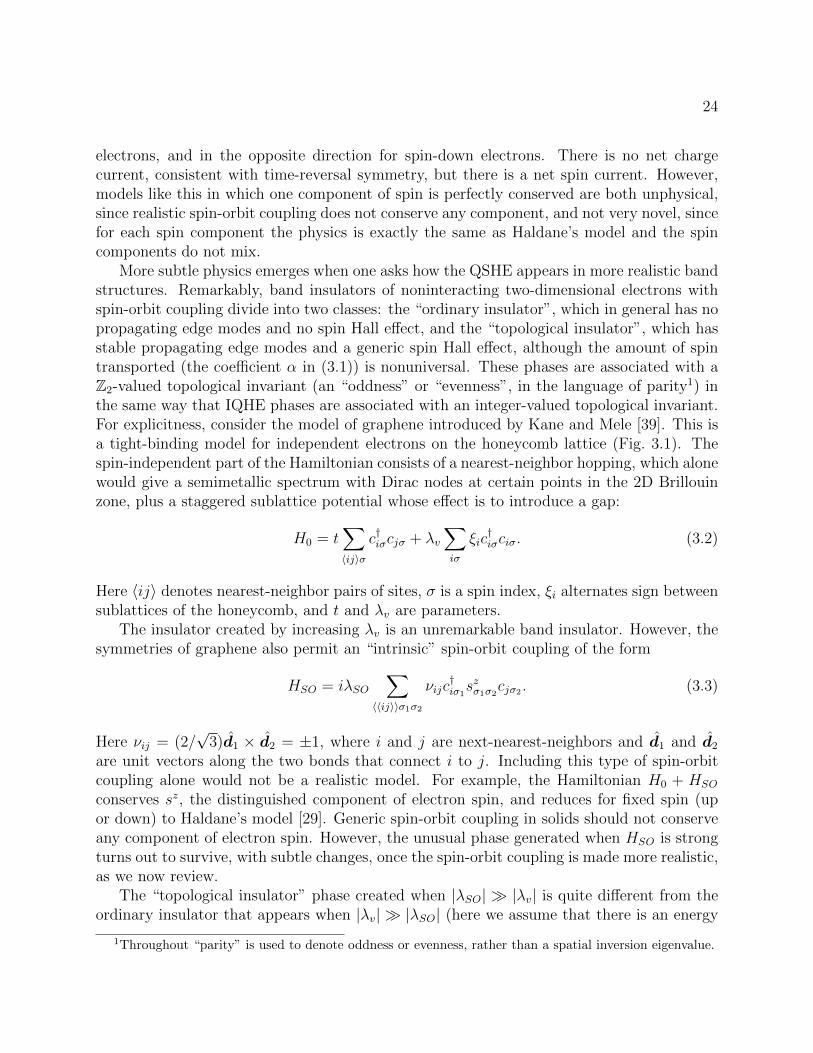
More subtle physics emerges when one asks how the QSHE appears in more realistic bandstructures. Remarkably, band insulators of noninteracting two-dimensional electrons withspin-orbit coupling divide into two classes: the “ordinary insulator”, which in general has nopropagating edge modes and no spin Hall effect, and the “topological insulator”, which hasstable propagating edge modes and a generic spin Hall effect, although the amount of spintransported (the coefficient α in (3.1)) is nonuniversal. These phases are associated with aZ2-valued topological invariant (an “oddness” or “evenness”, in the language of parity1) inthe same way that IQHE phases are associated with an integer-valued topological invariant.For explicitness, consider the model of graphene introduced by Kane and Mele [39]. This isa tight-binding model for independent electrons on the honeycomb lattice (Fig. 3.1). Thespin-independent part of the Hamiltonian consists of a nearest-neighbor hopping, which alonewould give a semimetallic spectrum with Dirac nodes at certain points in the 2D Brillouinzone, plus a staggered sublattice potential whose effect is to introduce a gap:

H0 = t∑〈ij〉σ

c†iσcjσ + λv∑iσ

ξic†iσciσ. (3.2)

Here 〈ij〉 denotes nearest-neighbor pairs of sites, σ is a spin index, ξi alternates sign betweensublattices of the honeycomb, and t and λv are parameters.

The insulator created by increasing λv is an unremarkable band insulator. However, thesymmetries of graphene also permit an “intrinsic” spin-orbit coupling of the form

HSO = iλSO∑

〈〈ij〉〉σ1σ2

νijc†iσ1szσ1σ2cjσ2 . (3.3)

Here νij = (2/√

3)d1 × d2 = ±1, where i and j are next-nearest-neighbors and d1 and d2

are unit vectors along the two bonds that connect i to j. Including this type of spin-orbitcoupling alone would not be a realistic model. For example, the Hamiltonian H0 + HSO

conserves sz, the distinguished component of electron spin, and reduces for fixed spin (upor down) to Haldane’s model [29]. Generic spin-orbit coupling in solids should not conserveany component of electron spin. However, the unusual phase generated when HSO is strongturns out to survive, with subtle changes, once the spin-orbit coupling is made more realistic,as we now review.

The “topological insulator” phase created when |λSO| |λv| is quite different from theordinary insulator that appears when |λv| |λSO| (here we assume that there is an energy

1Throughout “parity” is used to denote oddness or evenness, rather than a spatial inversion eigenvalue.

25

Ly

Lx

d1d2

ψeiφx

ψeiφx+iφyψeiφy

ψ

Figure 3.1: The honeycomb lattice on which the tight-binding Hamiltonian resides. For thetwo sites depicted, the factor νij of equation (3.3) is νij = −1. The phases φx,y describetwisted boundary conditions, introduced in equation (3.10).

gap between the lower and upper band pairs in which the Fermi level lies). The former hascounterpropagating edge modes and shows the QSHE, while the latter does not [39]. Doesthis phase exist for more realistic spin-orbit coupling? The spin component sz is no longera good quantum number when the Rashba spin-orbit coupling is added:

HR = iλR∑〈ij〉σ1σ2

c†iσ1

(sσ1σ2 × dij

)zcjσ2 , (3.4)

with dij the vector from i→ j and dij the corresponding unit vector. Note that Rashba spin-orbit coupling is not intrinsic to graphene but generated by inversion-symmetry breaking inthe out-of-plane direction [11]. The Rashba coupling is a standard form that is believed tobe a reasonable model for the dominant spin-orbit coupling in adsorbed graphene.

The topological insulator survives but is strongly modified in the presence of the Rashbaterm. For a general 2D band structure with sz conserved, there are many phases labeled byan integer n, as in the IQHE: if spin-up electrons are in the ν = n state, then spin-downelectrons must be in the ν = −n state by time-reversal symmetry, where the sign indicatesthat the direction of the effective magnetic field is reversed. Once sz is not conserved, as whenλR 6= 0, there are only two insulating phases, the “ordinary” and “topological” insulators.A heuristic definition of the topological insulator, without reference to any particular spincomponent or the spin Hall effect, is as a band insulator that is required to have gaplesspropagating edge modes at the sample boundaries. The decoupled ν = ±n cases with sz

conserved are adiabatically connected, once sz is not conserved, to the ordinary insulator foreven n and to the topological insulator for odd n. A review of how these two cases emergeas the only possibilities in 2D follows in Section II.

26

It should be clarified that the intrinsic spin-orbit coupling is now believed to be quite weakin graphene [38, 54, 92], so that the topological insulator is unlikely to be realized. However,the same topological insulator phase is now believed to exist for realistic spin-orbit couplingin other materials such as HgTe [8]. We choose to study the graphene model introducedby Kane and Mele because it is the first and simplest model showing a transition betweenordinary and topological insulators. It is the simplest possible model in that it has four spin-split bands, which is the minimum number required for the nontrivial phase to exist [56].For this reason, it has received the most attention in the other studies [75, 64] to which ourresults will be compared. It is straightforward to generalize the approach presented here forthe graphene model to another material with more complicated spin-orbit coupling, and thesame qualitative results are expected to apply.

It is not obvious at first glance how to generalize the topological insulator phase tofinite, noncrystalline systems, rather than band structures, as when the parameters of theHamiltonian H = H0 +HSO+HR are drawn from a random distribution. The first approachwas in terms of a spin Chern number [75] similar to the Chern integer in finite IQHE systems,but there is now agreement that for a clean band structure the only invariants are of Z2

type, rather than integer type [23, 56, 26]. Two equivalent definitions of the appropriateZ2 invariant for a finite disordered system, in the simple case when the disorder splits alldegeneracies other than Kramers degeneracies, are as follows (the full definition is given andcompared to previous work in the following section). The finite system can be consideredas a unit “supercell” of a large 2D lattice. A large, finite supercell gives many bands, buteach pair of bands connected by time reversal (Kramers pair) can be assigned its own Z2

invariant [56]. The phase of the supercell system, if the Fermi level lies in a gap, is thenidentified by adding up all the invariants (mod 2). Alternately, a direct definition of thephase in the finite system can be given that is related to the notion of “Z2 pumping” [23].Real charge is pumped as the flux through the system is taken from 0 to hc/2e (half the usualflux quantum that appears in IQHE pumping); we show that in the topological insulator,any pumping cycle, properly defined, pumps an odd number of electron charges, while forthe ordinary insulator any cycle pumps an even number of charges.

We implement this definition numerically using an explicit algorithm introduced by Fukuiand Hatsugai [26, 25] for computing Z2 topological invariants on a Brillouin zone. Thetopological insulator phase is robust to disorder: while different realizations of disorder assigndifferent “Chern parities” to individual subbands, it is found that the total for occupiedsubbands is always “odd” for a wide range of parameters, which in our definition indicates atopological insulator. In the IQHE, a pair of bands of opposite Chern number can annihilateas the strength of disorder is increased; in the QSHE, two band pairs that both have oddChern parity can annihilate, i.e., become two even-parity band pairs. If the topologicalinsulator can be destroyed by band annihilation, then there are extended (i.e., topologicallynontrivial) states with an arbitrarily small gap; it may be the case that for some range ofparameters, there are extended states at the Fermi level even in the thermodynamic limit,indicating a metallic phase.

In the IQHE, there is only a single energy with extended states rather than a range of

27

energies, and hence no metallic phase. We find the phase diagram of the graphene modelwith on-site disorder, and in the presence of non-zero Rashba coupling find evidence for ametallic phase intervening between ordinary and topological insulators. The existence of themetallic phase can be understood from work on 2D localization in the symplectic universalityclass [34], in which time-reversal symmetry is unbroken but spin-orbit coupling is present.It is found that extended states can be stable against this disorder over a nonzero range inenergy, unlike in the orthogonal class, in which there are no extended states, or the unitary(integer quantum hall) class, in which there are extended states only at isolated energies.The argument for the existence of the symplectic metal is beyond the scope of this work,but there is a simple picture that captures some of the important ideas.

Consider the question, what is the probability that a spinless electron will return to itsstarting point? In a path-integral picture, the amplitude associated with some return path γwill be Aγ. In the presence of disorder, this amplitude will interfere incoherently with thosefrom other paths, but it will interfere coherently with the time reversed path (i.e., the samepath traversed in the opposite direction), no matter how strong the disorder is. This givesan unnormalized probability |A + A|2 = 4|A|2. Hence the probability of return is enhancedrelative to the the probability to travel to the edge of the system and be lost, since there is notime-reversed path which with to interfere in that case. [2, 1] The situation is different withstrong spin-orbit coupling. If the spin is locked to the direction of motion, then there is aspin Berry phase that needs to be included with the amplitudes. In a remarkably simple andcomprehensible paper, Bergmann showed that this factor is −1/2 on average, due essentiallyto the fact that a spin-1/2 electron picks up a sign upon rotation through 2π. [7] That is,the interference is destructive rather than constructive, |A−A/2|2 = |A|2/4, and the spinfulelectron is more likely to pass through the sample than return to its starting point, leadingto a nonzero conductivity.

Our result that there is a metallic phase can be understood as indicating that, althoughthe Z2 topological invariant allows one to distinguish two kinds of insulators when the Fermilevel has no extended states, this invariant does not modify the standard picture of bandsof extended states in the symplectic universality class.

Recent work by Obuse et al. [63] obtains a phase diagram and critical exponents usinga network model for the spin quantum Hall effect that is similar to the Chalker-Coddingtonnetwork model [13] for the IQHE (see also Onoda et al. [64] for a quasi-1D study of local-ization in the Kane-Mele Hamiltonian with disorder). Our results on the phase diagram areconsistent with these works, although our method is unable to generate large enough sys-tem sizes to confirm the exponents found for the phase transitions. To understand how thenetwork and Chern-parity approaches complement each other, consider the integer quantumHall effect (IQHE): while the phenomenological network approach to the IQHE is valuableboth to find the critical indices precisely and to identify the minimal necessary elements of atheory for the transition, Chern-number studies remain important for studies of effects suchas the floating of extended states [47, 42, 90], where knowledge of the topological propertiesof a state is required. The network model gives more accurate information about the phasetransitions but, if only the localization length is probed, does not distinguish the different

28

phases in bulk. A more technical difference between the two approaches is discussed at theend of Section II.

Section II reviews how the topological insulator phase in perfect crystals arises from aparity-valued topological invariant of the band structure, similar to the TKNN [81] integersin the IQHE. It then gives two mathematically equivalent definitions of the topologicalinsulator phase in disordered systems based on Chern parity. One definition simply considersa finite disordered system as a supercell of an infinite lattice system, while the other isbased upon closed charge pumping cycles driven by application of flux to a finite periodicsystem. Section III reviews the Fukui-Hatsugai algorithm [26, 25] adapted to numericalcomputation of these invariants in disordered systems, then computes the phase diagramof the Kane-Mele graphene model [39] with on-site disorder. The conclusions of our studyfor general 2D disordered systems are summarized in a short Section IV. While there is athree-dimensional version of the QSHE [56, 72, 22] that is less directly connected to theIQHE and has interesting localization behavior, we will restrict our attention to 2D exceptfor some comments in the final section.

3.2 Chern parities for disordered noninteracting elec-

tron systems

3.2.1 The definition of the Z2 invariant in clean systems

We review one definition of the Z2 invariant of a band pair in a 2D band structure, thenexplain its generalization to noncrystalline systems. With the Hamiltonian

H = H0 +HSO +HR (3.5)

defined in equations (3.2), (3.3), and (3.4), or any periodic, single-electron Hamiltonian, aBerry connection A can be defined on the Brillouin zone (BZ) from the periodic part u(k)of a Bloch state ψk = u(k)eik·r. For a single nondegenerate band j, Aj(k) = −i〈uj|∇k|uj〉.This Berry connection serves as a potential for the Berry field strength F = (∇k×A)z, which,when integrated over the BZ, returns an integer, called a TKNN integer in the context ofthe IQHE [81]:

nj = − 1

2π

∫BZ

Fj d2k

=i

2π

∫BZ

[⟨∂u

∂kx

∣∣∣ ∂u∂ky

⟩−⟨∂u

∂ky

∣∣∣ ∂u∂kx

⟩]. (3.6)

When bands touch, only the total TKNN integer of the bands is well-defined [4], in whichcase it makes sense to generalize A as

Aj = −i (〈uj1|∇k|uj1〉+ 〈uj2|∇k|uj2〉)= −i truj

†∇kuj (3.7)

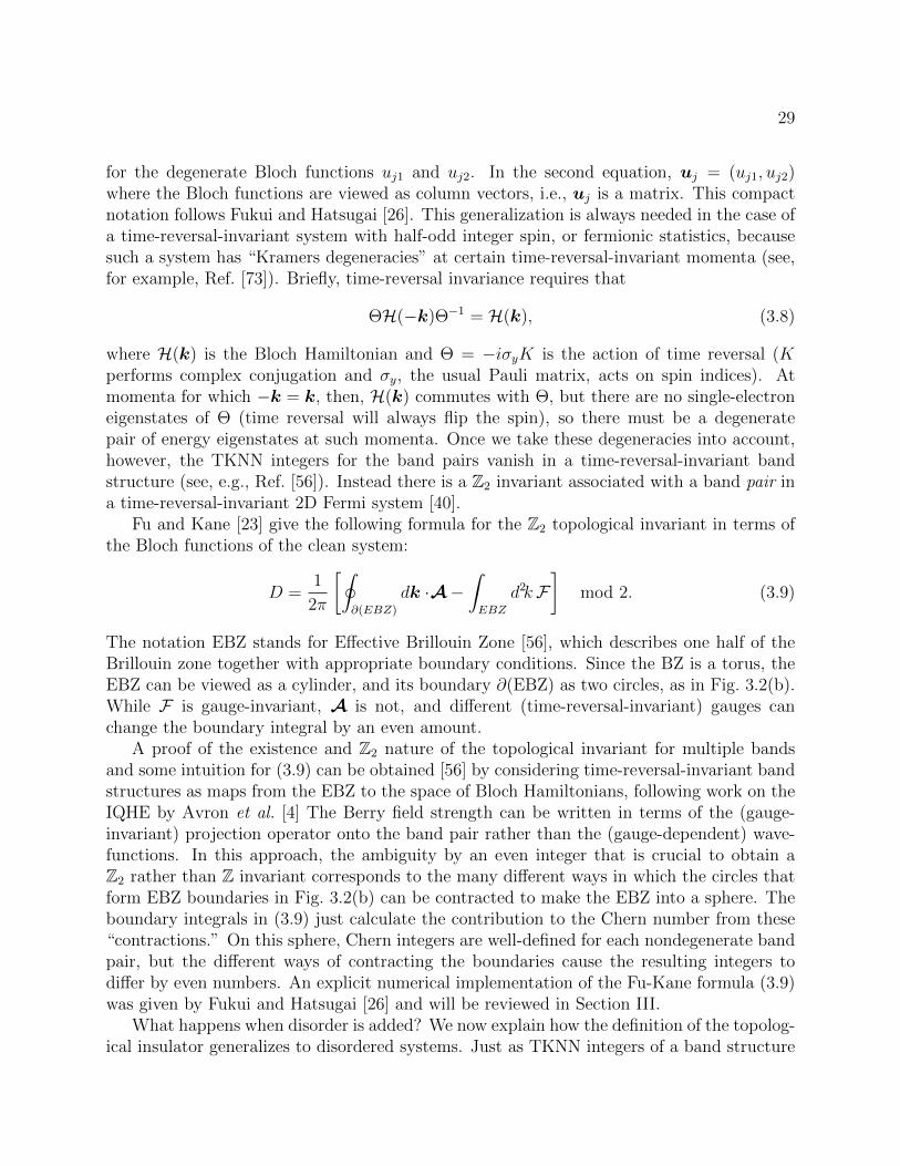
29

for the degenerate Bloch functions uj1 and uj2. In the second equation, uj = (uj1, uj2)where the Bloch functions are viewed as column vectors, i.e., uj is a matrix. This compactnotation follows Fukui and Hatsugai [26]. This generalization is always needed in the case ofa time-reversal-invariant system with half-odd integer spin, or fermionic statistics, becausesuch a system has “Kramers degeneracies” at certain time-reversal-invariant momenta (see,for example, Ref. [73]). Briefly, time-reversal invariance requires that

ΘH(−k)Θ−1 = H(k), (3.8)

where H(k) is the Bloch Hamiltonian and Θ = −iσyK is the action of time reversal (Kperforms complex conjugation and σy, the usual Pauli matrix, acts on spin indices). Atmomenta for which −k = k, then, H(k) commutes with Θ, but there are no single-electroneigenstates of Θ (time reversal will always flip the spin), so there must be a degeneratepair of energy eigenstates at such momenta. Once we take these degeneracies into account,however, the TKNN integers for the band pairs vanish in a time-reversal-invariant bandstructure (see, e.g., Ref. [56]). Instead there is a Z2 invariant associated with a band pair ina time-reversal-invariant 2D Fermi system [40].

Fu and Kane [23] give the following formula for the Z2 topological invariant in terms ofthe Bloch functions of the clean system:

D =1

2π

[∮∂(EBZ)

dk ·A−∫EBZ

d2kF]

mod 2. (3.9)

The notation EBZ stands for Effective Brillouin Zone [56], which describes one half of theBrillouin zone together with appropriate boundary conditions. Since the BZ is a torus, theEBZ can be viewed as a cylinder, and its boundary ∂(EBZ) as two circles, as in Fig. 3.2(b).While F is gauge-invariant, A is not, and different (time-reversal-invariant) gauges canchange the boundary integral by an even amount.

A proof of the existence and Z2 nature of the topological invariant for multiple bandsand some intuition for (3.9) can be obtained [56] by considering time-reversal-invariant bandstructures as maps from the EBZ to the space of Bloch Hamiltonians, following work on theIQHE by Avron et al. [4] The Berry field strength can be written in terms of the (gauge-invariant) projection operator onto the band pair rather than the (gauge-dependent) wave-functions. In this approach, the ambiguity by an even integer that is crucial to obtain aZ2 rather than Z invariant corresponds to the many different ways in which the circles thatform EBZ boundaries in Fig. 3.2(b) can be contracted to make the EBZ into a sphere. Theboundary integrals in (3.9) just calculate the contribution to the Chern number from these“contractions.” On this sphere, Chern integers are well-defined for each nondegenerate bandpair, but the different ways of contracting the boundaries cause the resulting integers todiffer by even numbers. An explicit numerical implementation of the Fu-Kane formula (3.9)was given by Fukui and Hatsugai [26] and will be reviewed in Section III.

What happens when disorder is added? We now explain how the definition of the topolog-ical insulator generalizes to disordered systems. Just as TKNN integers of a band structure

30

C

Γ

B

A

Γ

B

A

C

(a) (b)

-π/a π/a-π/a

π/a

0

0

Figure 3.2: (a) A two-dimensional Brillouin zone; note that any such Brillouin zone, includingthat for graphene, can be smoothly deformed to a torus. The labeled points are time-reversal-invariant momenta. (b) The effective Brillouin zone (EBZ). The horizontal lines onthe boundary circles ∂(EBZ) connect time-reversal-conjugate points, where the Hamiltoniansare related by time reversal and so cannot be specified independently.

give rise to Chern integers in a disordered system of finite size, the Z2 invariants of bandpairs become “Chern parities”.

3.2.2 The topological insulator phase for Slater determinants viaChern parity

The TKNN integers generalize in the presence of disorder and interactions to the Chernnumber of the many-particle wavefunction [62]. A natural question is how disorder andinteractions modify the Z2 invariants of band pairs in spin-orbit-coupled 2D band structures.All derivations of the Z2 invariants of clean systems depend on Fermi statistics in some way:for example, the existence of Kramers degeneracies and the related fact that the time-reversaloperator squares to −1 both depend on Fermi statistics. A many-fermion wavefunctiondescribing an even number of fermions does not behave in the same way as single-fermionwavefunctions under time-reversal. Hence, given only the many-fermion wavefunction, itdoes not seem likely that there is a generalization of the Z2 invariant.

However, for the particular case of many-fermion wavefunctions that are single Slaterdeterminants of single-particle wavefunctions, the invariant can be generalized as we nowshow. While the assumption of a single Slater determinant limits the treatment of interac-tions to the Hartree-Fock level, there is no requirement that the wavefunctions in the Slaterdeterminant be Bloch states. As a result, the topological insulator and QSHE can be definedand studied for any disorder strength.

Niu et al. [62] and Avron and Seiler [5] showed that for disordered quantum Hall systemsthere exists a generalization of the TKNN invariant defined for clean systems [81]. Theyintroduce generalized periodic boundary conditions and find an invariant Chern number,similar in form to the TKNN invariant, on the space of boundary phases. Consider a finitesystem of noninteracting electrons with boundary conditions that are periodic up to phases

31

φx, φy, as shown in Fig. 3.1: this is equivalent to putting magnetic fluxes Φx,y = φx,yΦ0/2πthrough the two noncontractible circles on the torus (Φ0 = hc/e is the magnetic flux quan-tum). As motivation, think of the finite system as a (possibly very large) unit cell of a latticesystem. Then in order to determine the phase of this lattice system, instead of integratingover k to do the integrals in the Fu-Kane formula (3.9), we integrate over the boundaryphases, which introduce offsets to the wave vectors. We now carry out this procedure, showthat it reproduces the band-structure result for clean systems, and then discuss a physicalpicture and its relation to previous definitions.

Consider the single-particle wavefunctions of a lattice Hamiltonian such as the graphenemodel on a finite lattice of size Lx × Ly (see Fig. 3.1). Instead of the physical boundaryconditions ψ(x+Lx,y) = ψ(x) for a single-particle wavefunction ψ, introduce the boundaryphases, or “twists”, φ = (φx, φy) via

ψ(x+Lx) = eiφxψ(x), ψ(x+Ly) = eiφyψ(x). (3.10)

Then a unitary transformation of the form

χ(x) = e−i(φxx/Lx+φyy/Ly)ψ(x) (3.11)

will transfer the twist angles to the Hamiltonian. Under the change of basis (3.11), Kane andMele’s model Hamiltonian [39] H = H0 + HSO + HR (see Section I) becomes (suppressingspinor indices)

H → H(φ) =∑〈ij〉

ci†[t+ iλR(s× dij)z

]cje−i∆·dij + iλSO

∑〈〈ij〉〉

νijci†szcje

−i∆·dij

+∑i

(λvξi + wi)ci†ci, (3.12)

where ∆ = (φx/Lx, φy/Ly), dij is still the vector i→ j, and we have added a random termfor on-site disorder, wi, drawn from the Gaussian distribution of zero mean and standarddeviation σw. It is now clear that under time reversal,

ΘH(−φ)Θ−1 = H(φ), (3.13)

since the extra phase factors in H change sign under complex conjugation.2 Since thisdirectly parallels equation (3.8), the Z2 invariant D of the Brillouin zone passes directly totwist space:

Dφ =1

2π

[∮∂(ETZ)

dφ ·A−∫ETZ

d2φF]

mod 2, (3.14)

2Note that this means H is not generically time-reversal invariant. Indeed, there are only four boundaryconditions that respect time-reversal, namely those for which ψ picks up a real phase upon translationaround each cycle of the honeycomb lattice. These four correspond to the TRIM of the clean system in thecalculation of D.

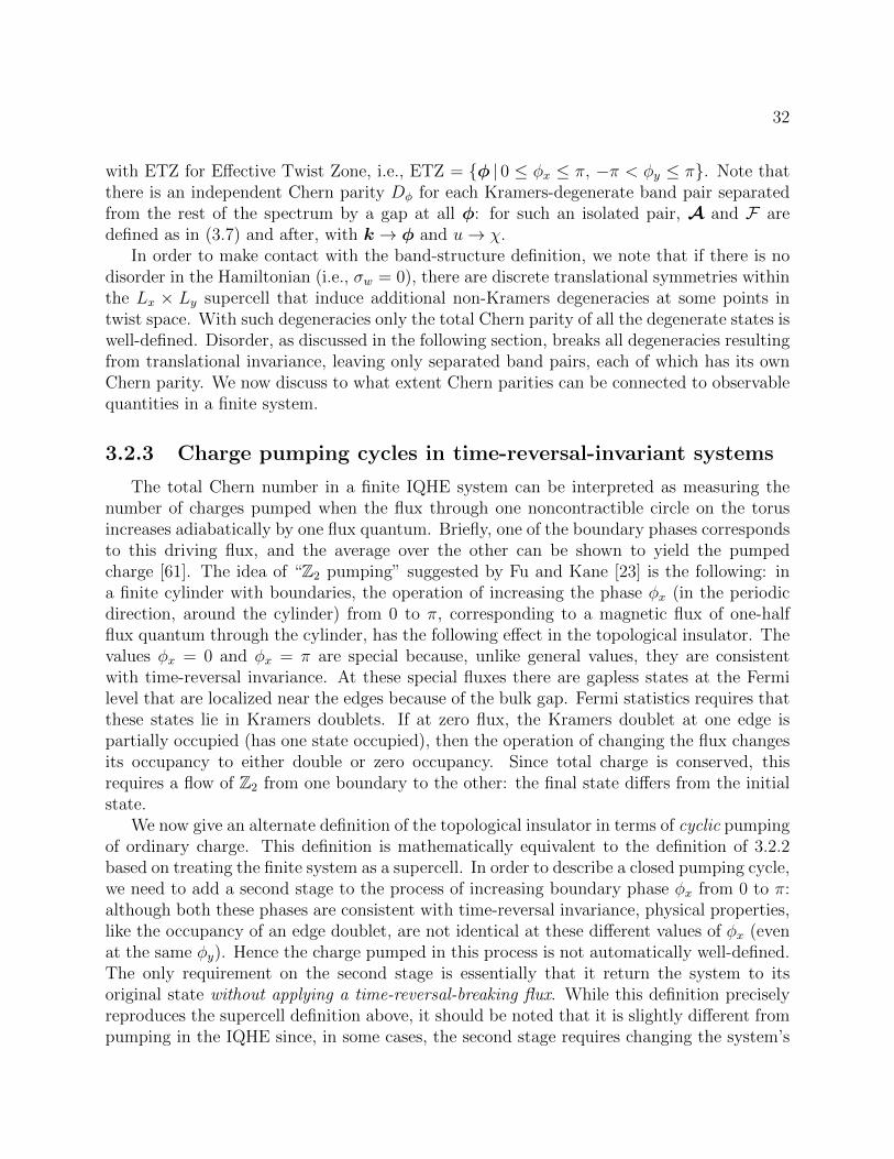
32

with ETZ for Effective Twist Zone, i.e., ETZ = φ | 0 ≤ φx ≤ π, −π < φy ≤ π. Note thatthere is an independent Chern parity Dφ for each Kramers-degenerate band pair separatedfrom the rest of the spectrum by a gap at all φ: for such an isolated pair, A and F aredefined as in (3.7) and after, with k→ φ and u→ χ.

In order to make contact with the band-structure definition, we note that if there is nodisorder in the Hamiltonian (i.e., σw = 0), there are discrete translational symmetries withinthe Lx × Ly supercell that induce additional non-Kramers degeneracies at some points intwist space. With such degeneracies only the total Chern parity of all the degenerate states iswell-defined. Disorder, as discussed in the following section, breaks all degeneracies resultingfrom translational invariance, leaving only separated band pairs, each of which has its ownChern parity. We now discuss to what extent Chern parities can be connected to observablequantities in a finite system.

3.2.3 Charge pumping cycles in time-reversal-invariant systems

The total Chern number in a finite IQHE system can be interpreted as measuring thenumber of charges pumped when the flux through one noncontractible circle on the torusincreases adiabatically by one flux quantum. Briefly, one of the boundary phases correspondsto this driving flux, and the average over the other can be shown to yield the pumpedcharge [61]. The idea of “Z2 pumping” suggested by Fu and Kane [23] is the following: ina finite cylinder with boundaries, the operation of increasing the phase φx (in the periodicdirection, around the cylinder) from 0 to π, corresponding to a magnetic flux of one-halfflux quantum through the cylinder, has the following effect in the topological insulator. Thevalues φx = 0 and φx = π are special because, unlike general values, they are consistentwith time-reversal invariance. At these special fluxes there are gapless states at the Fermilevel that are localized near the edges because of the bulk gap. Fermi statistics requires thatthese states lie in Kramers doublets. If at zero flux, the Kramers doublet at one edge ispartially occupied (has one state occupied), then the operation of changing the flux changesits occupancy to either double or zero occupancy. Since total charge is conserved, thisrequires a flow of Z2 from one boundary to the other: the final state differs from the initialstate.

We now give an alternate definition of the topological insulator in terms of cyclic pumpingof ordinary charge. This definition is mathematically equivalent to the definition of 3.2.2based on treating the finite system as a supercell. In order to describe a closed pumping cycle,we need to add a second stage to the process of increasing boundary phase φx from 0 to π:although both these phases are consistent with time-reversal invariance, physical properties,like the occupancy of an edge doublet, are not identical at these different values of φx (evenat the same φy). Hence the charge pumped in this process is not automatically well-defined.The only requirement on the second stage is essentially that it return the system to itsoriginal state without applying a time-reversal-breaking flux. While this definition preciselyreproduces the supercell definition above, it should be noted that it is slightly different frompumping in the IQHE since, in some cases, the second stage requires changing the system’s

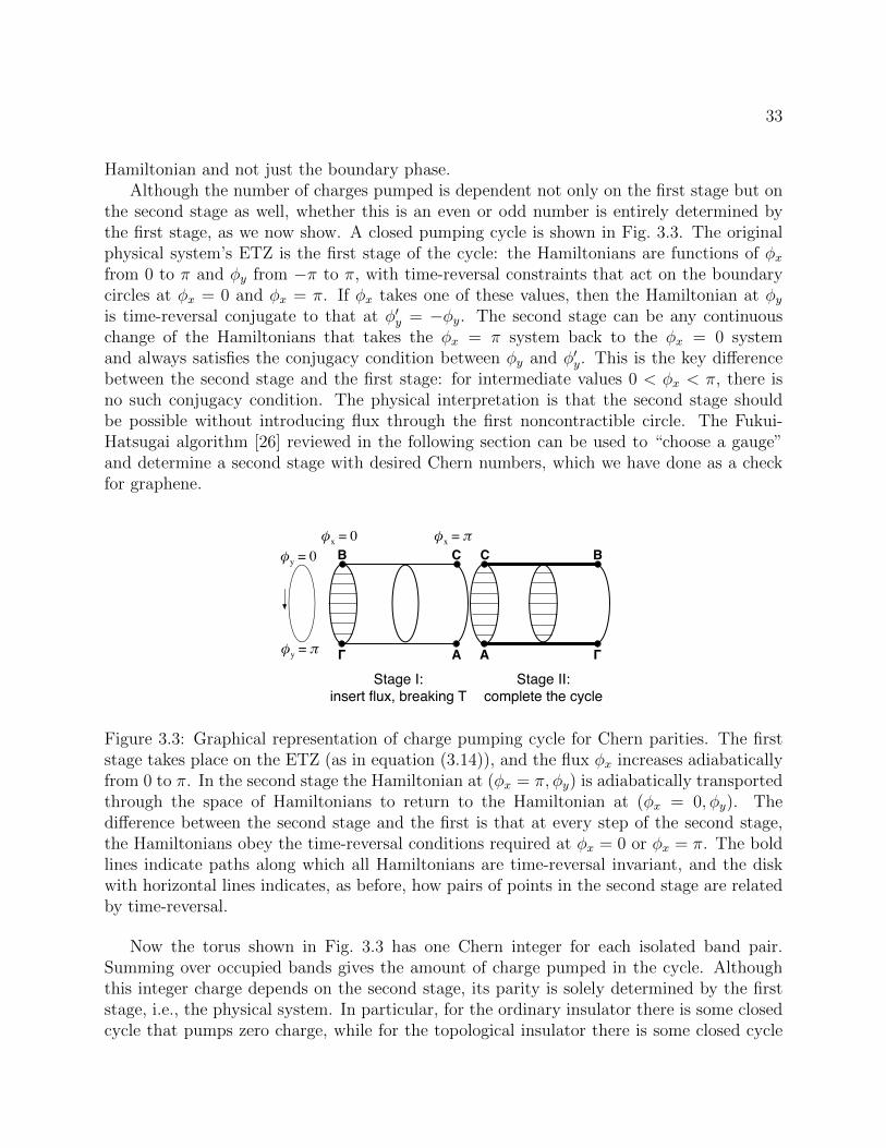
33

Hamiltonian and not just the boundary phase.Although the number of charges pumped is dependent not only on the first stage but on

the second stage as well, whether this is an even or odd number is entirely determined bythe first stage, as we now show. A closed pumping cycle is shown in Fig. 3.3. The originalphysical system’s ETZ is the first stage of the cycle: the Hamiltonians are functions of φxfrom 0 to π and φy from −π to π, with time-reversal constraints that act on the boundarycircles at φx = 0 and φx = π. If φx takes one of these values, then the Hamiltonian at φyis time-reversal conjugate to that at φ′y = −φy. The second stage can be any continuouschange of the Hamiltonians that takes the φx = π system back to the φx = 0 systemand always satisfies the conjugacy condition between φy and φ′y. This is the key differencebetween the second stage and the first stage: for intermediate values 0 < φx < π, there isno such conjugacy condition. The physical interpretation is that the second stage shouldbe possible without introducing flux through the first noncontractible circle. The Fukui-Hatsugai algorithm [26] reviewed in the following section can be used to “choose a gauge”and determine a second stage with desired Chern numbers, which we have done as a checkfor graphene.

Γ

B

A

C

A

C B

Stage I:insert flux, breaking T

Γ

φx = 0 φx = π

Stage II:complete the cycle

φy = 0

φy = π

Figure 3.3: Graphical representation of charge pumping cycle for Chern parities. The firststage takes place on the ETZ (as in equation (3.14)), and the flux φx increases adiabaticallyfrom 0 to π. In the second stage the Hamiltonian at (φx = π, φy) is adiabatically transportedthrough the space of Hamiltonians to return to the Hamiltonian at (φx = 0, φy). Thedifference between the second stage and the first is that at every step of the second stage,the Hamiltonians obey the time-reversal conditions required at φx = 0 or φx = π. The boldlines indicate paths along which all Hamiltonians are time-reversal invariant, and the diskwith horizontal lines indicates, as before, how pairs of points in the second stage are relatedby time-reversal.

Now the torus shown in Fig. 3.3 has one Chern integer for each isolated band pair.Summing over occupied bands gives the amount of charge pumped in the cycle. Althoughthis integer charge depends on the second stage, its parity is solely determined by the firststage, i.e., the physical system. In particular, for the ordinary insulator there is some closedcycle that pumps zero charge, while for the topological insulator there is some closed cycle

34

Topological Insulator

Ordinary Insulator

λSO

λRλR

λv

OrdinaryInsulator

TopologicalInsulator

a. b.

Topological Insulator

Metal

Ordinary Insulator

λSO

λR

c.

IQHEIQHE

Figure 3.4: Schematic phase diagram. (a) Phase diagram for a clean system, with fixed t andλSO 6= 0 (after Kane and Mele [40]). (b) Again a clean system, now with fixed t and λv 6= 0.(c) The expected form of the phase diagram at nonzero disorder (we run all simulations atfixed λv). The phase boundary in (b) opens up into a metallic phase, closing only whenλR = 0, where there should be an IQHE transition.

that pumps unit charge. These results follow from the same proof as for the band structurecase in Ref. [56]: one shows that the differences in resulting Chern integers between anytwo second stages are even. The pumping definition gives a different physical picture forthe “contractions” introduced there; instead of contracting the EBZ to a sphere, here theETZ is contracted to a torus by adding the second stage. The technical reason that thesetwo constructions are equivalent is that, since the appropriate spaces of Hamiltonians arecontractible (i.e., have π1 = 0), the two closed manifolds, the torus and the sphere, bothhave the same topological invariants, namely integer-valued Chern numbers.

The topological insulator in disordered systems has been studied previously by locatingthe transition between topological and ordinary insulators as a point or region where thelocalization length of single-electron eigenstates diverges. The existence of the topologicalinsulator is inferred from the existence of this transition region (or alternately from the edgestates in the topological insulator phase). In principle this approach could give a differentresult from ours, in that our definition probes the existence not just of extended states butspecifically of extended states that contribute to the pumping of charge, or alternately thatcan give rise to edge states. The same distinction arises in the quantum Hall effect, wherelooking for extended states of nonzero Chern number is a more direct probe of quantum Hallphysics than considering the inverse participation ratio, for example, which would detectextended states of zero Chern number in addition to topological states. However, as in thequantum Hall case, we find that the phase boundaries from our Chern-parity definition areconsistent with those obtained from calculations of the localization length [64, 63].

35

3.3 Graphene Model and Numerics

3.3.1 The phase diagram of the disordered graphene model

It is useful to review some general expectations before applying the definitions of theprevious section to study a disordered version of the graphene model. In two-dimensionalsystems with time-reversal invariance and no spin-orbit coupling, even very weak disorderwill localize electron wavefunctions, so that these systems do not ever conduct in the ther-modynamic limit. In the presence of a magnetic field, as in the IQHE, there are isolatedenergies with extended states, but no finite-width range of energies with extended states,and hence no true metallic phase. Hikami et al. showed [34] that disordered two-dimensionalsystems with spin-orbit coupling can nevertheless support a metallic phase, referred to as a“symplectic metal”. They calculated ladder diagrams for the problem of random potentialscattering in 2D in order to obtain a renormalization-group equation for the resistance, andfound that, in the presence of strong spin-orbit scattering without magnetic scattering (sothat the system is time-reversal invariant), the resistance flows to zero, indicating extendedstates and a metallic phase. In the presence of strong magnetic scattering (i.e., the IQHE),by contrast, the resistance does not flow at that order, and at next order grows (see alsoRef. [33]).

In the case studied here, any metallic phase induced by disorder would presumably appearin a region around the parameter set that closes the (clean) gap, as depicted schematically inFig. 3.4. At λR = 0 the z component of spin is a good quantum number (sz commutes withH), so the system reduces to two copies of the Haldane model [29], which has a quantumHall plateau transition with no metallic phase. Hence when λR = 0 there should be a directtransition between insulators even with disorder.

3.3.2 Lattice Implementation

For numerical work we use the algorithm of Fukui and Hatsugai, which we reviewhere [26]. The formula (3.9) for D requires a gauge choice for the Hamiltonian eigenstatesat each φ on the two boundaries of the half-torus 0 ≤ φx ≤ π, −π < φy ≤ π. That is, the“field strength” F is gauge invariant, but the gauge potential A is not. The eigenstates formKramers pairs related by time reversal, and the gauge choice must respect this constraint.

Now, at the time-reversal invariant points φ = (0, 0), (0, π), (π, 0), and (π, π), the solidpoints in Fig. 3.5, the spectrum is degenerate, with two states at each energy. The gaugecondition requires that Θ interchange the two with a phase factor e±iπ/2 (so that Θ2 = −1as required for single-fermion states). Numerical diagonalization will not, in general, returneigenvectors that obey this condition, but we can force them to do so as follows: choosingone of the two members of each Kramers pair at energy ε2n−1 = ε2n and calling that vectorχ2n−1, we discard the other and replace it by

χ2n = Θχ2n−1. (3.15)

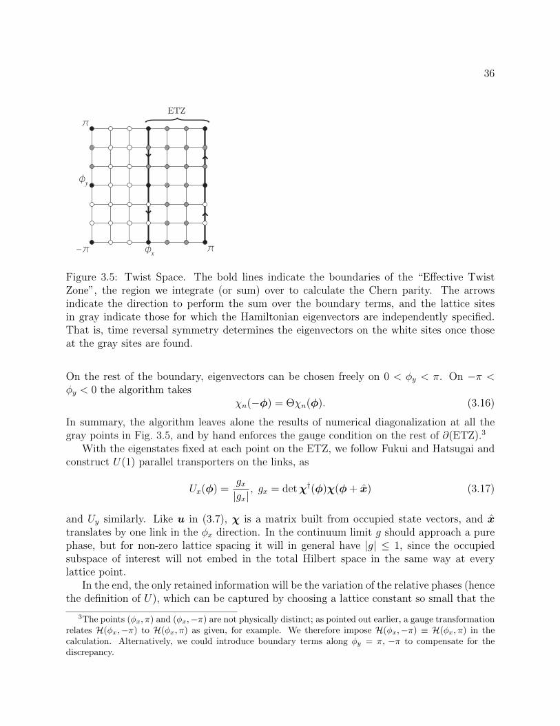
36

π

π

−π φx

φy

ETZFigure 3.5: Twist Space. The bold lines indicate the boundaries of the “Effective TwistZone”, the region we integrate (or sum) over to calculate the Chern parity. The arrowsindicate the direction to perform the sum over the boundary terms, and the lattice sitesin gray indicate those for which the Hamiltonian eigenvectors are independently specified.That is, time reversal symmetry determines the eigenvectors on the white sites once thoseat the gray sites are found.

On the rest of the boundary, eigenvectors can be chosen freely on 0 < φy < π. On −π <φy < 0 the algorithm takes

χn(−φ) = Θχn(φ). (3.16)

In summary, the algorithm leaves alone the results of numerical diagonalization at all thegray points in Fig. 3.5, and by hand enforces the gauge condition on the rest of ∂(ETZ).3

With the eigenstates fixed at each point on the ETZ, we follow Fukui and Hatsugai andconstruct U(1) parallel transporters on the links, as

Ux(φ) =gx|gx|

, gx = detχ†(φ)χ(φ+ x) (3.17)

and Uy similarly. Like u in (3.7), χ is a matrix built from occupied state vectors, and xtranslates by one link in the φx direction. In the continuum limit g should approach a purephase, but for non-zero lattice spacing it will in general have |g| ≤ 1, since the occupiedsubspace of interest will not embed in the total Hilbert space in the same way at everylattice point.

In the end, the only retained information will be the variation of the relative phases (hencethe definition of U), which can be captured by choosing a lattice constant so small that the

3The points (φx, π) and (φx,−π) are not physically distinct; as pointed out earlier, a gauge transformationrelates H(φx,−π) to H(φx, π) as given, for example. We therefore impose H(φx,−π) ≡ H(φx, π) in thecalculation. Alternatively, we could introduce boundary terms along φy = π, −π to compensate for thediscrepancy.

37

phase field varies slowly over one link. However, the scale of variation will presumably differfor different disorder realizations, and we would like a way to diagnose this and throw outthose realizations for which fast variation makes the calculation unreliable. The phase isperiodic, and if it were to wind through 2π over the distance of one link the algorithm wouldmiss this fact, so the relative phase will not provide a good diagnostic. As a proxy, we chooseto cull out disorder realizations that result in small determinants in most simulations, sincea small overlap between adjacent occupied eigenspaces indicates rapid variation. Of course,this filtering could introduce a selection bias into the results; these effects are within thestatistical uncertainty of our analysis (in particular, within the error bars of Fig. 3.9).

Associated with the transporter on each link is a gauge potential Ax,y = logUx,y. ThisA is pure imaginary, and the logarithm is defined to return the branch A/i ∈ (−π, π).Associated with the transport around each plaquette is a flux

F (φ) = logUx(φ)Uy(φ+ x)U−1x (φ+ y)U−1y (φ), (3.18)

again satisfying F/i ∈ (−π, π). With these definitions in hand, the lattice Z2 invariantcorresponding to Dφ (3.14) is

DL =1

2πi

∑|∈∂(ETZ)

Ay −∑

∈ETZ

F

mod 2. (3.19)

Of course, the sum over the boundary should have the same orientation as the correspondingcontour integral in (3.14); in Fig. 3.5, this means the sum on the left boundary should carry aminus sign, following the arrows. As mentioned previously, this formalism has the desirableproperty of guaranteeing that DL = 0or1, but using too coarse a mesh can return the wrongvalue.

3.3.3 Numerical Results

As noted after equation (3.14), the number of nondegenerate Kramers pairs in a disor-dered system will generically be extensive, and we can use equation (3.19) to calculate theChern parity of each pair separately. Fig. 3.6 shows the results of such calculations on a4×6 lattice to present a picture of the three phases: normal insulator, symplectic metal, andtopological insulator. In all phases, there are Kramers pairs with Dφ = 1 in the lower half ofthe energy spectrum, as indicated by the bars. However, in the normal insulator (λSO wellbelow the transition, or gap closure) there are an even number of such pairs in the occupiedhalf of all realizations, so that the overall Chern parity is even. The presence of a very smallnumber of realizations (2 of 215 for a 6× 8 lattice) with odd parity indicates either the tailof the disorder-broadened transition or, more likely, that the weak filter applied for thesesimulations failed to catch all realizations with rapidly varying link variables.

When λSO is large, almost all realizations have an odd number of Z2-odd Kramers pairs(as with the small-λSO case, 2 realizations do not follow the rule), and in the region near the

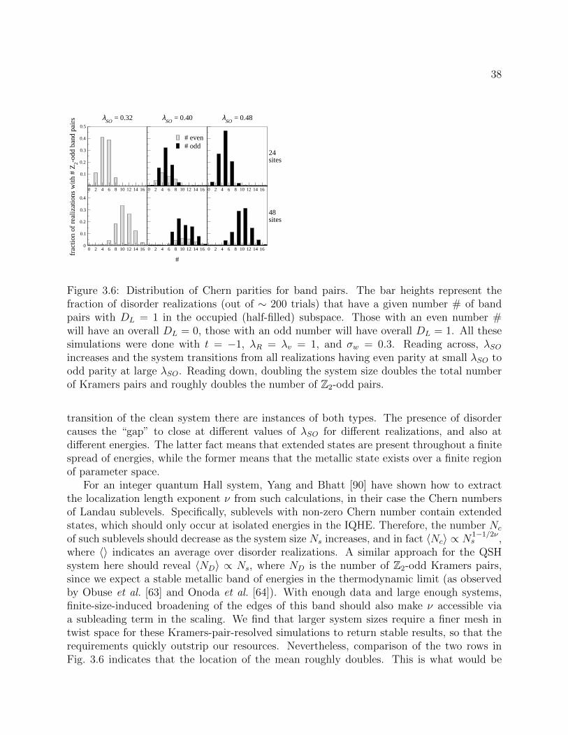
38

0 2 4 6 8 10 12 14 16

0.1

0.2

0.3

0.4

0.5

λSO = 0.32

0 2 4 6 8 10 12 14 16

# even# odd

λSO = 0.40

0 2 4 6 8 10 12 14 16

24sites

λSO = 0.48

0 2 4 6 8 10 12 14 16

48sites

0 2 4 6 8 10 12 14 16

#0 2 4 6 8 10 12 14 16

0

0.1

0.2

0.3

0.4

frac

tion

of re

aliz

atio

ns w

ith #

Z2-o

dd b

and

pairs

Figure 3.6: Distribution of Chern parities for band pairs. The bar heights represent thefraction of disorder realizations (out of ∼ 200 trials) that have a given number # of bandpairs with DL = 1 in the occupied (half-filled) subspace. Those with an even number #will have an overall DL = 0, those with an odd number will have overall DL = 1. All thesesimulations were done with t = −1, λR = λv = 1, and σw = 0.3. Reading across, λSOincreases and the system transitions from all realizations having even parity at small λSO toodd parity at large λSO. Reading down, doubling the system size doubles the total numberof Kramers pairs and roughly doubles the number of Z2-odd pairs.

transition of the clean system there are instances of both types. The presence of disordercauses the “gap” to close at different values of λSO for different realizations, and also atdifferent energies. The latter fact means that extended states are present throughout a finitespread of energies, while the former means that the metallic state exists over a finite regionof parameter space.

For an integer quantum Hall system, Yang and Bhatt [90] have shown how to extractthe localization length exponent ν from such calculations, in their case the Chern numbersof Landau sublevels. Specifically, sublevels with non-zero Chern number contain extendedstates, which should only occur at isolated energies in the IQHE. Therefore, the number Nc

of such sublevels should decrease as the system size Ns increases, and in fact 〈Nc〉 ∝ N1−1/2νs ,

where 〈〉 indicates an average over disorder realizations. A similar approach for the QSHsystem here should reveal 〈ND〉 ∝ Ns, where ND is the number of Z2-odd Kramers pairs,since we expect a stable metallic band of energies in the thermodynamic limit (as observedby Obuse et al. [63] and Onoda et al. [64]). With enough data and large enough systems,finite-size-induced broadening of the edges of this band should also make ν accessible viaa subleading term in the scaling. We find that larger system sizes require a finer mesh intwist space for these Kramers-pair-resolved simulations to return stable results, so that therequirements quickly outstrip our resources. Nevertheless, comparison of the two rows inFig. 3.6 indicates that the location of the mean roughly doubles. This is what would be

39

expected for the middle case given the above considerations; the mean for the topologicalinsulator (the right-hand panels in Fig. 3.6) should grow more slowly, as in the case studiedby Yang and Bhatt.

The total phase of the system, given by the total Chern parity, is more relevant topossible measurements than the Chern parity of each Kramers pair. The former maintainsits meaning if we consider the ground state wave function of the many-electron system,formed as a Slater determinant of the single-electron states we use here. There is also acomputational benefit to calculating Dφ for the whole occupied subspace rather than forindividual pairs, as well — at larger system sizes, and also at stronger disorder, the linkvariables for the half-filled subspace vary much more slowly than those for the individualKramers pairs, making the calculation more robust. For these reasons the remaining plotsin this paper depict only the Chern parity of the half-filled system.

To show that a metallic region of non-zero extent in parameter space exists in the ther-modynamic limit, we need to verify that the mixed-phase region does not shrink to zero aswe increase the system size. Figure 3.7(a) shows that as we make the system larger, thetransition region certainly does not get narrower, and in fact the largest system size seemsto have the broadest transition.

We can quantify the scaling of the metallic region’s width with system size by assuminga simple one-parameter scaling form for the curves in Fig. 3.7(a) and defining the widthof the curve to be proportional to the reciprocal of the maximum slope: width ∼ 1/slope.With sufficient data, one could expand the approximately linear region near the middle ofthe transition in a power series with a few coefficients as fit parameters. Since our simulationdata are limited, we opt instead to assume the form (tanhα(s) + 1)/2, which has roughlythe right shape. If α = m(λSO − λ∗SO), then m is exactly the maximum slope we want.Figure 3.7(b) plots the data versus the best-fit scaling variable α for each system size; thepoints appear to fill out a smooth curve, justifying the scaling hypothesis. The best fitfor m and λ∗SO is determined by minimizing a weighted χ2 statistic [91]. In particular, weassume that the results (DL = ±1) of independent simulations at a fixed parameter set aredistributed binomially, and that for each system size there are the same number of trials ateach value of λSO (which is roughly true). In that case, the variance of the distribution canbe estimated as σ2 ∝ p(1− p) [15], where p is the fraction of disorder realizations returningDL = 1, and then 1/σ2 is an appropriate weight for the statistical test. The error bars inFigs. 3.7 and 3.8 are also assigned based on a binomial model of the data [91].

By contrast, at λR = 0 the Hamiltonian (3.5) reduces to two copies of the Haldane modeland so should exhibit the quantum Hall plateau transition, which looks like a step functionat zero temperature in the thermodynamic limit. In Fig. 3.8(a) the width of the transitionregion shrinks as the system size grows, consistent with the prediction.

More quantitatively, Pruisken [66] has shown in a renormalization group framework thatthe functional form of the crossover for the IQHE looks like

p(L,B) = f(α), α ∝ L1/ν(B −B∗), (3.20)

where L is the linear size of the finite sample, B is the applied magnetic field, and ν is

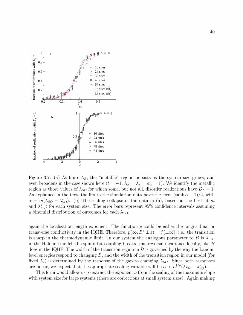
40

0.2 0.3 0.4 0.5λSO

0.2

0.4

0.6

0.8

1

frac

tion

of re

aliz

atio

ns w

ith D

L =

1

16 sites24 sites36 sites48 sites64 sites16 sites (fit)64 sites (fit)

-4 -2 0 2 4α

0.5

1

frac

tion

of re

aliz

atio

ns w

ith D

L =

1

16 sites24 sites36 sites48 sites64 sites

b.

a.

Figure 3.7: (a) At finite λR, the “metallic” region persists as the system size grows, andeven broadens in the case shown here (t = −1, λR = λv = σw = 1). We identify the metallicregion as those values of λSO for which some, but not all, disorder realizations have DL = 1.As explained in the text, the fits to the simulation data have the form (tanhα + 1)/2, withα = m(λSO − λ∗SO). (b) The scaling collapse of the data in (a), based on the best fit mand λ∗SO) for each system size. The error bars represent 95% confidence intervals assuminga binomial distribution of outcomes for each λSO.

again the localization length exponent. The function p could be either the longitudinal ortransverse conductivity in the IQHE. Therefore, p(∞, B∗ ± ε) = f(±∞), i.e., the transitionis sharp in the thermodynamic limit. In our system the analogous parameter to B is λSO:in the Haldane model, the spin-orbit coupling breaks time-reversal invariance locally, like Bdoes in the IQHE. The width of the transition region in B is governed by the way the Landaulevel energies respond to changing B, and the width of the transition region in our model (forfixed λv) is determined by the response of the gap to changing λSO. Since both responsesare linear, we expect that the appropriate scaling variable will be α ∝ L1/ν(λSO − λ∗SO).

This form would allow us to extract the exponent ν from the scaling of the maximum slopewith system size for large systems (there are corrections at small system sizes). Again making

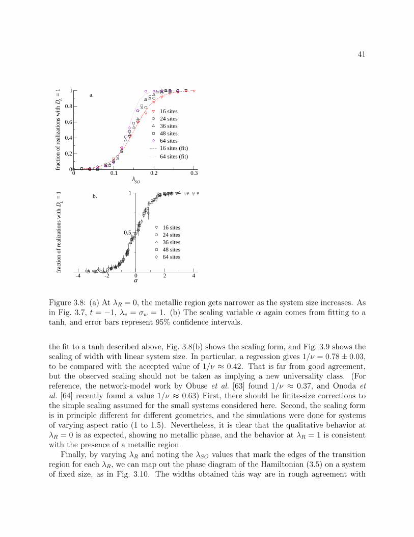
41

-4 -2 0 2 4α

0.5

1

frac

tion

of re

aliz

atio

ns w

ith D

L =

1

16 sites24 sites36 sites48 sites64 sites

0 0.1 0.2 0.3λSO

0

0.2

0.4

0.6

0.8

1

frac

tion

of re

aliz

atio

ns w

ith D

L =

1

16 sites24 sites36 sites48 sites64 sites16 sites (fit)64 sites (fit)

a.

b.

Figure 3.8: (a) At λR = 0, the metallic region gets narrower as the system size increases. Asin Fig. 3.7, t = −1, λv = σw = 1. (b) The scaling variable α again comes from fitting to atanh, and error bars represent 95% confidence intervals.

the fit to a tanh described above, Fig. 3.8(b) shows the scaling form, and Fig. 3.9 shows thescaling of width with linear system size. In particular, a regression gives 1/ν = 0.78± 0.03,to be compared with the accepted value of 1/ν ≈ 0.42. That is far from good agreement,but the observed scaling should not be taken as implying a new universality class. (Forreference, the network-model work by Obuse et al. [63] found 1/ν ≈ 0.37, and Onoda etal. [64] recently found a value 1/ν ≈ 0.63) First, there should be finite-size corrections tothe simple scaling assumed for the small systems considered here. Second, the scaling formis in principle different for different geometries, and the simulations were done for systemsof varying aspect ratio (1 to 1.5). Nevertheless, it is clear that the qualitative behavior atλR = 0 is as expected, showing no metallic phase, and the behavior at λR = 1 is consistentwith the presence of a metallic region.

Finally, by varying λR and noting the λSO values that mark the edges of the transitionregion for each λR, we can map out the phase diagram of the Hamiltonian (3.5) on a systemof fixed size, as in Fig. 3.10. The widths obtained this way are in rough agreement with

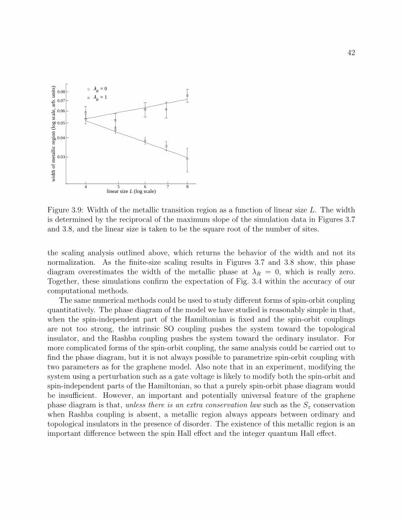
42

4 5 6 7 8linear size L (log scale)

0.03

0.04

0.05

0.06

0.07

0.08

wid

th o

f met

allic

regi

on (l

og sc

ale,

arb

. uni

ts) λR = 0

λR = 1

Figure 3.9: Width of the metallic transition region as a function of linear size L. The widthis determined by the reciprocal of the maximum slope of the simulation data in Figures 3.7and 3.8, and the linear size is taken to be the square root of the number of sites.

the scaling analysis outlined above, which returns the behavior of the width and not itsnormalization. As the finite-size scaling results in Figures 3.7 and 3.8 show, this phasediagram overestimates the width of the metallic phase at λR = 0, which is really zero.Together, these simulations confirm the expectation of Fig. 3.4 within the accuracy of ourcomputational methods.

The same numerical methods could be used to study different forms of spin-orbit couplingquantitatively. The phase diagram of the model we have studied is reasonably simple in that,when the spin-independent part of the Hamiltonian is fixed and the spin-orbit couplingsare not too strong, the intrinsic SO coupling pushes the system toward the topologicalinsulator, and the Rashba coupling pushes the system toward the ordinary insulator. Formore complicated forms of the spin-orbit coupling, the same analysis could be carried out tofind the phase diagram, but it is not always possible to parametrize spin-orbit coupling withtwo parameters as for the graphene model. Also note that in an experiment, modifying thesystem using a perturbation such as a gate voltage is likely to modify both the spin-orbit andspin-independent parts of the Hamiltonian, so that a purely spin-orbit phase diagram wouldbe insufficient. However, an important and potentially universal feature of the graphenephase diagram is that, unless there is an extra conservation law such as the Sz conservationwhen Rashba coupling is absent, a metallic region always appears between ordinary andtopological insulators in the presence of disorder. The existence of this metallic region is animportant difference between the spin Hall effect and the integer quantum Hall effect.

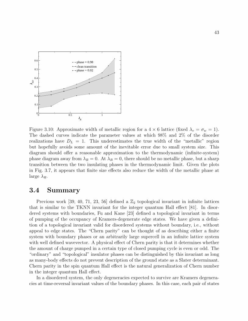
43

0 0.5 1λR

0

0.1

0.2

0.3

0.4

0.5

0.6

λ SO

phase = 0.98clean transitionphase = 0.02

Figure 3.10: Approximate width of metallic region for a 4 × 6 lattice (fixed λv = σw = 1).The dashed curves indicate the parameter values at which 98% and 2% of the disorderrealizations have DL = 1. This underestimates the true width of the “metallic” regionbut hopefully avoids some amount of the inevitable error due to small system size. Thisdiagram should offer a reasonable approximation to the thermodynamic (infinite-system)phase diagram away from λR = 0. At λR = 0, there should be no metallic phase, but a sharptransition between the two insulating phases in the thermodynamic limit. Given the plotsin Fig. 3.7, it appears that finite size effects also reduce the width of the metallic phase atlarge λR.

3.4 Summary

Previous work [39, 40, 71, 23, 56] defined a Z2 topological invariant in infinite latticesthat is similar to the TKNN invariant for the integer quantum Hall effect [81]. In disor-dered systems with boundaries, Fu and Kane [23] defined a topological invariant in termsof pumping of the occupancy of Kramers-degenerate edge states. We have given a defini-tion of a topological invariant valid for disordered systems without boundary, i.e., withoutappeal to edge states. The “Chern parity” can be thought of as describing either a finitesystem with boundary phases or an arbitrarily large supercell in an infinite lattice systemwith well defined wavevector. A physical effect of Chern parity is that it determines whetherthe amount of charge pumped in a certain type of closed pumping cycle is even or odd. The“ordinary” and “topological” insulator phases can be distinguished by this invariant as longas many-body effects do not prevent description of the ground state as a Slater determinant.Chern parity in the spin quantum Hall effect is the natural generalization of Chern numberin the integer quantum Hall effect.

In a disordered system, the only degeneracies expected to survive are Kramers degenera-cies at time-reversal invariant values of the boundary phases. In this case, each pair of states

44

related by Kramers degeneracies can be assigned its own Chern parity, and the overall Chernparity of all occupied state pairs determines the observable phase. The lattice algorithm forZ2 topological invariants laid out by Fukui and Hatsugai [26, 25] allugows numerical iden-tification of the topological insulator phase in disordered QSH systems. Implementing thisalgorithm for the specific graphene model Hamiltonian of Kane and Mele [40] with addedon-site disorder, we observe the ordinary and topological insulator phases in simulations.While the number of “odd” pairs (state pairs with odd Chern parity) varies with the disor-der realization, there is an even number of odd pairs in the ordinary insulator, and an oddnumber of odd pairs in the topological insulator.

We find that a metallic phase opens up between the two insulating phases for genericspin-orbit coupling. This agrees with the prediction of Hikami et al. [34] that spin-orbitcoupling can protect a 2D metallic phase from disorder, and confirms the simulation resultsof Onoda et al. [64] and Obuse et al. [63] The methods in this paper could in principle beused to study the three-dimensional case and confirm the argument in Ref. [24] that only oneof the four invariants of a band structure [56, 72, 22] is stable to disorder. While there is nowstrong evidence [63] that the phase transitions in the 2D QSHE are, except for special points,in the previously studied symplectic metal-insulator class, there is as yet no numerical studyof the phase transitions in three-dimensional topological insulators.

45

Chapter 4

Magnetoelectric polarizability andaxion electrodynamics in crystallineinsulators

The previous chapter dealt with the two-dimensional topological insulator, and showedthat its topological invariant can be generalized to the case of finite samples with disorder.It also verified that the combination of spin-orbit coupling and disorder lead to a metallicphase in two dimensions. There are also three-dimensional topological insulators, whichhave a topological invariant that can be built from the 2d invariant already discussed. This(shorter) chapter uses an alternative formulation, in which the topological invariant is aphysical response function, the magnetoelectric polarizability.

Magnetoelectric couplings in solids have recently been the subject of intense experimentaland theoretical investigations [77, 21, 32]. A quantity of central importance is the linearmagnetoelectric polarizability αij defined via

αij =∂Mj

∂Ei

∣∣∣B=0

=∂Pi∂Bj

∣∣∣E=0

(4.1)

where E and B are electric and magnetic fields, P and M are the polarization and magneti-zation, and the equality can be obtained from commuting derivatives of an appropriate freeenergy. In general the tensor α has nine independent components, and can be decomposedas

αij = αij +θe2

2πhδij (4.2)

where the first term is traceless and the second term, written here in terms of the dimension-less parameter θ, is the pseudoscalar part of the coupling. Here we focus on magnetoelectriccoupling resulting from the orbital (frozen-lattice) magnetization and polarization, which welabel the orbital magnetoelectic polarizability (OMP).

In field theory, the pseudoscalar OMP coupling is said to generate “axion electrodynam-

46

ics” [82], and corresponds to a Lagrangian of the form (c = 1)

∆LEM =θe2

2πhE ·B =

θe2

16πhεαβγδFαβFγδ. (4.3)

An essential feature of the axion theory is that, when the axion field θ(r, t) is constant,it plays no role in electrodynamics; this follows because θ couples to a total derivative,εαβγδFαβFγδ = 2εαβγδ∂α(AβFγδ), and so does not modify the equations of motion. However,the presence of the axion field can have profound consequences at surfaces and interfaces,where gradients in θ(r) appear.

A second essential feature is that electrodynamics is invariant under θ → θ + 2π [82]. Inorder to reconcile this peculiar fact with the phenomenology of the magnetoelectric effect,observe that the axion coupling can alternatively be described in terms of a surface Hallconductivity σH whose value θe2/2πh is determined by bulk properties, but only modulothe quantum e2/h. More generally, at an interface between two samples, σH = (θ1 − θ2 +2πr)e2/2πh, where the integer r depends on the details of the interface. Recall that, ingeneral, a 2D gapped crystal has an integer TKNN invariant C in terms of which the itsHall conductivity is σH = Ce2/h [81]. The “modulo e2/h”, or integer r, discussed abovecorresponds to modifying the surface or interface by adsorbing a surface layer of nonzero C.

When time-reversal (T ) invariance is present, the TKNN invariants vanish, but other in-variants arise that have been the focus of much recent work. In 2D there is a Z2 invariant [40]distinguishing “ordinary” from “Z2-odd” insulators, with “quantum spin Hall” states [39, 8]providing examples of the latter. In 3D there is a similar invariant [56, 72, 22] that canbe computed either from the 2D invariant on certain planes [56] or from an index involvingthe eight T -invariant momenta [22]. If this is odd, the material is a “strong topologicalinsulator” (STI). In the context of the OMP, note that T maps θ → −θ; the ambiguity of θmodulo 2π then implies that T invariance is consistent with either θ = 0 or θ = π, with thelatter corresponding to the STI [67]. Note that if T -invariance extends to the surfaces, thesebecome metallic by virtue of topologically protected edge states, as observed experimentallyfor the Bi0.9Sb0.1 system [37]. If the surface is gapped by a T -breaking perturbation, thenσH = e2/h modulo 2e2/h at the surface of a STI [82, 24, 67].

In the noninteracting case, a Berry-phase expression for θ has been given in terms of thebulk bandstructure by Qi, Hughes, and Zhang [67] by integrating out electrons in one higherdimension. Defining the Berry connection Aµνj = i〈uµ|∂j|uν〉 where |uν〉 is the cell-periodicBloch function of occupied band ν and ∂j = ∂/∂kj, they obtain

θ = − 1

4π

∫BZ

d3k εijk Tr[Ai∂jAk − i2

3AiAjAk] (4.4)

where the trace is over occupied bands.In the present letter, we first provide an alternate derivation of Eq. (4.4) for the OMP.

Our derivation clarifies that θ is a polarizability and in fact describes the entire orbital con-tribution to magnetoelectric polarizability. That is, the orbital α vanishes in Eq. (4.2), and

47

the orbital contribution is a perfect pseudoscalar. The derivation follows from an extension[87] of the Berry-phase theory of polarization [43] to the case of slow spatial variations ofthe Hamiltonian. (Indeed, the OMP angle θ is a bulk property in exactly the same sense aselectric polarization [65, 43].) We find that the OMP can be generalized to the interactingcase and calculated from the many-particle wavefunction, even though Eq. (4.4) is not valid;this reflects a subtle difference between OMP and polarization. Explicit numerical calcu-lations on model crystals are presented to validate the theory, establish the equivalence ofEq. (4.4) to the prior definition, and illustrate how a non-zero θ corresponds to a “fractional”quantum Hall effect at the surface of a magnetoelectric or topological insulator [82, 24, 67].

From Eq. (4.1) it is evident that the OMP can be viewed in several ways. (i) It describesthe electric polarization arising from the application of a small magnetic field. (ii) It describesthe orbital magnetization arising from the application of a small electric field. (iii) It alsogives the (dissipationless) surface Hall conductivity σH at the surface of the crystal, providedthat the surface is insulating. Note that (iii) follows from (ii): for a surface with unit normaln and electric field E, the resulting surface current K = M × n is proportional to E × n.There is an elegant analogy here to the case of electric polarization, where the surface chargeof an insulating surface is determined, modulo the quantum e/S, by the bulk bandstructurealone (S is the surface cell area).

The above discussion suggests two approaches to deriving a bulk formula for the OMP θ.One is to follow (ii) and compute the orbital magnetization [78, 88] in an applied electricalfield. We focus here on (i) instead, working via dP/dB. The modern theory of polariza-tion starts from the polarization current jP = dP/dt under slow deformation of the BlochHamiltonian, and contains, to first order in d/dt, one power of the Berry curvature definedbelow [43]. Using semiclassical wavepacket dynamics, Xiao et al. [87] have shown how tocompute the polarization current to second order and to incorporate slow spatial variationsin the electronic Hamiltonian. For the case of an orthorhombic 3D crystal with M occupiedbands in which the slow spatial variation occurs along the y direction in a supercell of lengthly, they obtain

〈∆P (in)x 〉=

e

8

∫ 1

0

dλ

∫BZ

d3k

(2π)3

∫ ly

0

dy

lyεijklTr[FijFkl] (4.5)

for the change in the supercell-averaged inhomogeneously induced polarization that occurs asa global parameter λ evolves adiabatically from 0 to 1. Here indices ijkl run over (kx, ky, y, λ),Fij = ∂iAj − ∂jAi − i[Ai,Aj] is the Berry curvature tensor (Aµνλ = i〈uµ|∂λ|uν〉), and thetrace and commutator refer to band indices.

Because F is gauge-covariant, the integrand in Eq. (4.5) is explicitly gauge-invariant;it is the non-Abelian second Chern class [60], so that Eq. (4.5) is path-invariant modulo aquantum e/azly, where az is the lattice constant in the z direction. Moreover, the λ integralcan be performed to obtain an expression in terms of the non-Abelian Chern-Simons 3-form[60]. Thus,

〈P (in)x 〉 = −e

2

∫BZ

d3k

(2π)3

∫ ly

0

dy

lyεijkTr[Ai∂jAk −

2i

3AiAjAk] (4.6)

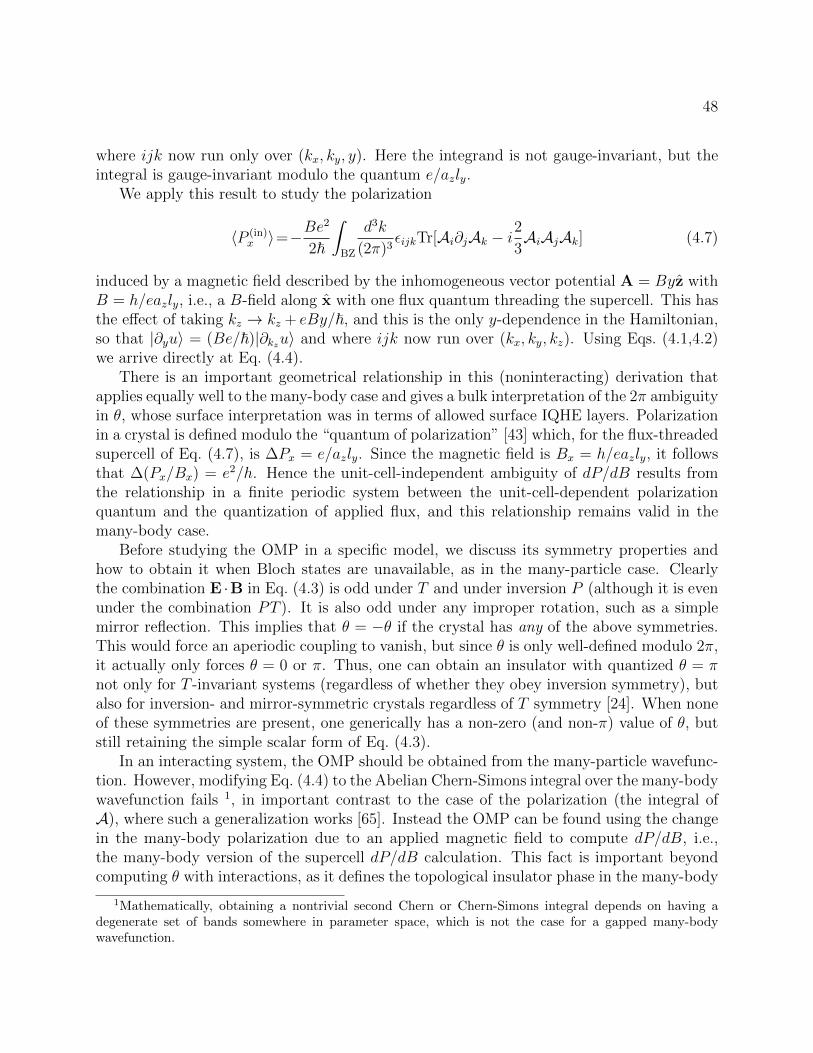
48

where ijk now run only over (kx, ky, y). Here the integrand is not gauge-invariant, but theintegral is gauge-invariant modulo the quantum e/azly.

We apply this result to study the polarization

〈P (in)x 〉=−

Be2

2~

∫BZ

d3k

(2π)3εijkTr[Ai∂jAk − i

2

3AiAjAk] (4.7)

induced by a magnetic field described by the inhomogeneous vector potential A = Byz withB = h/eazly, i.e., a B-field along x with one flux quantum threading the supercell. This hasthe effect of taking kz → kz + eBy/~, and this is the only y-dependence in the Hamiltonian,so that |∂yu〉 = (Be/~)|∂kzu〉 and where ijk now run over (kx, ky, kz). Using Eqs. (4.1,4.2)we arrive directly at Eq. (4.4).

There is an important geometrical relationship in this (noninteracting) derivation thatapplies equally well to the many-body case and gives a bulk interpretation of the 2π ambiguityin θ, whose surface interpretation was in terms of allowed surface IQHE layers. Polarizationin a crystal is defined modulo the “quantum of polarization” [43] which, for the flux-threadedsupercell of Eq. (4.7), is ∆Px = e/azly. Since the magnetic field is Bx = h/eazly, it followsthat ∆(Px/Bx) = e2/h. Hence the unit-cell-independent ambiguity of dP/dB results fromthe relationship in a finite periodic system between the unit-cell-dependent polarizationquantum and the quantization of applied flux, and this relationship remains valid in themany-body case.

Before studying the OMP in a specific model, we discuss its symmetry properties andhow to obtain it when Bloch states are unavailable, as in the many-particle case. Clearlythe combination E ·B in Eq. (4.3) is odd under T and under inversion P (although it is evenunder the combination PT ). It is also odd under any improper rotation, such as a simplemirror reflection. This implies that θ = −θ if the crystal has any of the above symmetries.This would force an aperiodic coupling to vanish, but since θ is only well-defined modulo 2π,it actually only forces θ = 0 or π. Thus, one can obtain an insulator with quantized θ = πnot only for T -invariant systems (regardless of whether they obey inversion symmetry), butalso for inversion- and mirror-symmetric crystals regardless of T symmetry [24]. When noneof these symmetries are present, one generically has a non-zero (and non-π) value of θ, butstill retaining the simple scalar form of Eq. (4.3).

In an interacting system, the OMP should be obtained from the many-particle wavefunc-tion. However, modifying Eq. (4.4) to the Abelian Chern-Simons integral over the many-bodywavefunction fails 1, in important contrast to the case of the polarization (the integral ofA), where such a generalization works [65]. Instead the OMP can be found using the changein the many-body polarization due to an applied magnetic field to compute dP/dB, i.e.,the many-body version of the supercell dP/dB calculation. This fact is important beyondcomputing θ with interactions, as it defines the topological insulator phase in the many-body

1Mathematically, obtaining a nontrivial second Chern or Chern-Simons integral depends on having adegenerate set of bands somewhere in parameter space, which is not the case for a gapped many-bodywavefunction.

49

case more simply than before [48]. Like the IQHE, the topological insulator is defined viaa response function (dP/dB) to a perturbation that, in the limit of a large system withperiodic boundary conditions, is locally weak and hence does not close the insulating gap.In the IQHE, this response function is to a boundary phase (i.e., a flux that does not passthrough the 2D system), while for the topological insulator, the defining response is to amagnetic flux through the 3D system.

In the remainder of this Letter, we demonstrate the above theory via numerical cal-culations on a tight-binding Hamiltonian that generates non-zero values of θ, then discussexperimental measurements of θ. We start with the model of Fu, Kane, and Mele [22] for a3D topological insulator on the diamond lattice,

HFKM =∑〈ij〉

tijc†icj + i

4λSOa2

∑〈〈ij〉〉

c†iσ · (d1ij × d2

ij)cj. (4.8)

In the first term, the nearest-neighbor hopping amplitude depends on the bond direction;we take tij = 3t + δ for direction [111] (in the conventional fcc unit cell of linear size a)and tij = t for the other three bonds. The second term describes spin-dependent hoppingbetween pairs of second neighbors 〈〈ij〉〉, where d1

ij and d2ij are the connecting first-neighbor

legs and σ are the Pauli spin matrices. With |δ| < 2t and λSO sufficiently large, this modelhas a direct band gap of 2|δ|.

To break T we add a staggered Zeeman field with opposite signs on the two fcc sublattices

A and B, h ·(∑

i∈A c†iσci −

∑i∈B c

†iσci

). We take |h| = m sin β and choose h in the [111]

direction; setting δ = m cos β and varying the single parameter β keeps the gap constant andinterpolates smoothly between the ordinary (β = 0) and the topological (β = π) insulator.

We have calculated the OMP angle θ using four different methods with excellent agree-ment (Fig. 4.1). First, we obtain θ from Eq. (4.4); this requires a smooth gauge for A,which can be found using now-standard Wannier-based methods [52]. Results are shown forβ = π/4 and β = π/2 (filled squares).

Next, we have calculated the polarization [43]

Pi = e

∫BZ

d3k

(2π)3TrAi . (4.9)

resulting from a single magnetic flux quantum in a large supercell. Varying the supercellsize (and thereby B) allows us to approximate dP/dB, yielding the open squares in Fig. 4.1.The points in Fig. 4.1 are from the surface Hall response in a slab geometry, describedbelow. Finally, to obtain the curve in Fig. 4.1, we also computed θ(β) from the secondChern expression [87, 67]

θ =1

16π

∫ β

0

dβ′∫d3k εijklTr[Fij(k, β′)Fkl(k, β′)] (4.10)

(derived above as Eq. (4.5)). Clearly, the various approaches are numerically equivalent.

50

è

è

èè

à

à

á

á

á

Π4 Π2 3Π4 ΠΒ

Π4

Π2

3Π4

ΠΘ

Figure 4.1: The magnetoelectric polarizability θ (in units of e2/2πh). The filled squaresare computed by the Chern-Simons form, Eq. (4.4). The open squares are dP/dB fromEq. (4.9). The points are obtained by layer-resolved σH calculations using Eq. (4.12). Thecurve is obtained from Eq. (4.10).

We now discuss the surface Hall conductivity, whose fractional part in units of e2/h isjust θ/2π [82]. Consider a material with coupling θ in a slab geometry that is finite inthe z direction and surrounded by θ = 0 vacuum. The simplest interfaces will then leadto σH = θe2/(2πh) at the top surface and −θe2/(2πh) at the bottom surface, for a totalσxy of zero. More generally, arbitrary surface quantum Hall layers change the total integerquantum Hall state, but not the fractional parts at each surface.

The spatial contributions to the Hall conductance in the slab geometry can be resolvedas follows. The unit cell is a supercell containing some number N of original unit cells in thez direction, with translational invariance remaining in the x and y directions. The TKNNinteger for the entire slab is [81, 4]

C =i

2π

∫d2kTr [Pεij∂iP∂jP ] . (4.11)

Here i and j take the values kx and ky and P =∑

ν |uν〉〈uν | is the projection operatoronto the occupied subspace (ν runs over occupied bands). To find how different z layerscontribute to C, define a projection Pn onto layer n within the supercell, and compute

C(n) =i

2π

∫d2kTr

[Pεij(∂iP)Pn(∂jP)

]. (4.12)

The results, presented in Fig. 4.2, confirm that the surface layers have half-integer Hallconductance when β = π in (4.8) and that the sign on each surface is switched by localT -breaking perturbations (in this example, a uniform Zeeman coupling in the surface layer).

To gain some insight into the microscopic origin of θ in the noninteracting case, usingEq. (4.4) we have calculated θ for a Hamiltonian that breaks PT (as well as P and T ) byadding a weak, uniform (i.e., not staggered) Zeeman coupling. For some values of β thislifts all degeneracies, enabling us to isolate the single-band and interband contributions to θ.

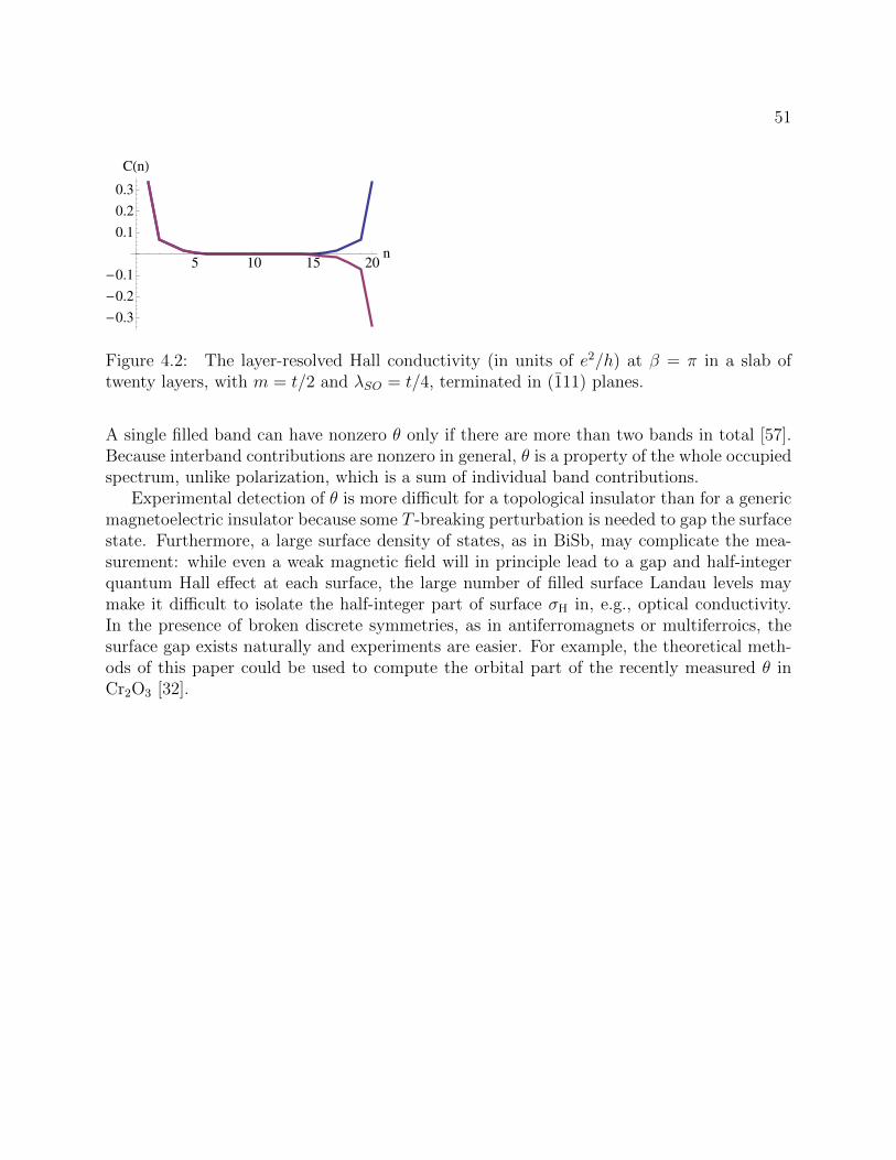
51

5 10 15 20n

-0.3

-0.2

-0.1

0.1

0.2

0.3

CHnL

Figure 4.2: The layer-resolved Hall conductivity (in units of e2/h) at β = π in a slab oftwenty layers, with m = t/2 and λSO = t/4, terminated in (111) planes.

A single filled band can have nonzero θ only if there are more than two bands in total [57].Because interband contributions are nonzero in general, θ is a property of the whole occupiedspectrum, unlike polarization, which is a sum of individual band contributions.

Experimental detection of θ is more difficult for a topological insulator than for a genericmagnetoelectric insulator because some T -breaking perturbation is needed to gap the surfacestate. Furthermore, a large surface density of states, as in BiSb, may complicate the mea-surement: while even a weak magnetic field will in principle lead to a gap and half-integerquantum Hall effect at each surface, the large number of filled surface Landau levels maymake it difficult to isolate the half-integer part of surface σH in, e.g., optical conductivity.In the presence of broken discrete symmetries, as in antiferromagnets or multiferroics, thesurface gap exists naturally and experiments are easier. For example, the theoretical meth-ods of this paper could be used to compute the orbital part of the recently measured θ inCr2O3 [32].

52

Interlude: magnetoelectric responseof a finite material

The previous chapter gave a semiclassical derivation of the Chern-Simons term in themagnetoelectric polarizability in a bulk insulator. Before proceeding to the full, and fullyquantum mechanical, derivation of the orbital magnetoelectric response in the next chapter,it is worth recording the result in a finite (insulating) sample of material. These results canalso be found in Malashevich et al. [51]. To linear order in the magnetic field, the (explicitlyHermitian) Hamiltonian is

Htot = H − 1

2(j ·A + A · j) = H − 1

2ji, Ai. (4.13)

We use curly braces , for the anticommutator. A convenient gauge for the vector potentialA is

Ai =1

2εijkB

jrk, (4.14)

where εijk is the fully antisymmetric Levi-Civita symbol. This gives

∂BjHtot =1

4εjabja, rb (4.15)

The response of the electronic polarization will then be

αij = ∂Bj

〈eri〉Ω

=1

Ω

∑n occ

〈n|eri|∂Bjn〉+ c.c. (4.16)

=eεjab2Ω

Re∑n occ

〈n|riG(En)ja, rb|n〉

=eεjab2Ω

Re∑n occ,l

〈n|ri|l〉〈l|ja, rb|n〉En − El + iε

,

where G(En) = (En − H + iε)−1 is the Schrodinger Green function for the unperturbedHamiltonian. We here take e to be the sign of the charge carrier, so it is negative forelectrons; Ω is the volume of the material in question. Observe that the real part of the sumover occupied states l vanishes automatically, which is to say, there is effectively a factor

53

1− f(El), where f(E) is the Fermi-Dirac distribution at zero temperature. Leaving the sumin this form is not helpful numerically, but it makes plain that α is a band-by-band sum ofa single-band response function, a property we shall call band additivity.

In an infinite system, the position is unbounded, and in a system with periodic (Born-vonKarman) boundary conditions it is either multivalued or discontinuous, implying that theexpression we have used for the electronic polarization, 〈er〉, is of questionable validity insuch cases. On the other hand, the current is perfectly well behaved, making it preferableto work with the current operator when possible. The two are related in the unperturbedsystem by

j =e

i[r, H], (4.17)

or in the basis of energy eigenstates,

〈l′|r|l〉 =ie

〈l′|j|l〉El − El′

. (4.18)

Matrix elements between occupied and unoccupied states are finite, then, because of thegap, while potential problems only appear in those between the (possibly degenerate) occu-pied states, making it worthwhile to separate out those contributions to α that have suchproblematic matrix elements. Using Eq. (4.18) and [ri, rj] = 0 it follows that

αij =eεjab

ΩRe

∑n occ

m unocc

〈n|ri|m〉〈m|ja(1− ρ)rb|n〉+ 〈m|rbρja|n〉

En − Em

+ie2

3Ωδijεabc

∑n,n′,n′′occ

〈n|ra|n′〉〈n′|rb|n′′〉〈n′′|rc|n〉. (4.19)

Here ρ is the projector onto the occupied states, otherwise known as the Fermi-Dirac densitymatrix at zero temperature, and 1− ρ is the complementary projector onto the unoccupiedstates. Note that the first sum looks very like Eq. (4.16) but with a factor of 2 difference.Remarkably, the troublesome (diagonal) matrix elements of r only contribute to the tracepart of the magnetoelectric tensor, that is, to θ.

That is to say, the first term presented has a simple generalization to infinite and/orperiodic systems. The second term does not, and is therefore the piece of most interest here.Let us rewrite it in terms of the density matrix as

(αCS)ij =ie2

3ΩδijεabcTrρraρrbρrc =

ie2

3ΩδijεabcTrρ[ρ, ra][ρ, rb]ρrc (4.20)

Ignoring the prefactors, this looks very much like a measure of volume, Tr(ρr) · (ρr)× (ρr),and evidently gives a measure of the “quantum volume” of the state ρ. Unfortunately, itdoes not seem to be possible to express it solely in terms of the noncommutative positionoperator r = i[ρ, r].

54

An alternative interpretation is as a polarization of Hall conductivities, since these aregiven by εabcρ[ρ, ra][ρ, rb]ρ. This formulation is essentially equivalent to reading off the re-sponse from the surface conductivity as was done in the last chapter. In the chapter tofollow, the derivation of the orbital magnetoelectric response is given in full for an infinite(boundaryless) system. The results look very similar to those derived here, and allow us toconclude that the “quantum volume” introduced here corresponds precisely to the Chern-Simons integral derived earlier from the semiclassical equations of motion.

55

Chapter 5

General orbital magnetoelectriccoupling in band insulators

5.1 Introduction

Understanding the response of a solid to applied magnetic or electric fields is of both fun-damental and applied interest. Two standard examples are that metals can be distinguishedfrom insulators by their screening of an applied electric field, and superconductors from met-als by their exclusion of magnetic field (the Meissner effect). Magnetoelectric response ininsulators has been studied for many years and is currently undergoing a renaissance drivenby the availability of new materials. The linear response of this type is the magnetoelectricpolarizability: in “multiferroic” materials that break parity and time-reversal symmetries,an applied electric field creates a magnetic dipole moment and a magnetic field creates anelectric dipole moment, and several applications have been proposed for such responses. Suchresponses are observed in a variety of materials and from a variety of mechanisms [77, 21].From a theoretical point of view, the most intriguing part of the polarizability is that due tothe orbital motion of electrons, because the orbital motion couples to the vector potentialrather than the more tangible magnetic field.

The orbital magnetoelectric polarizability has also been studied recently in non-magneticmaterials known as “topological insulators.” These insulators have Bloch wavefunctions withunusual topological properties, that lead to a magnetoelectric response described by an E ·Bterm in their effective electromagnetic Lagrangians, [67] with a quantized coefficient. Qi,Hughes, and Zhang [67] (QHZ) gave a formula for the coefficient of this term. For thespecific case of topological band insulators, their result reproduces earlier formulas for therelevant topological invariant, [22, 56, 72] but it is more generally valid: it describes acontribution to the magnetoelectric polarizability non just in topological insulators but inany band insulator. Their formula has a periodicity or ambiguity by e2/h that is related tothe possibility of surface quantum Hall layers on a three-dimensional sample and generalizesthe ambiguity of ordinary polarization.

56

The same E · B coupling, known as “axion electrodynamics” and originally studied inthe 1980s, [82] was obtained in a previous paper by three of the present authors [20] usinga semiclassical approach [87] to compute dP/dB, the polarization response to an appliedmagnetic field. However, in a general material, that semiclassical approach leads to anexplicit formula for only part of the orbital magnetoelectric polarizability, the part found byQHZ. [67] The remainder, which is generically nonvanishing in materials that break inversionand time-reversal symmetries, is expressed only implicitly in terms of the modification of theBloch wavefunctions by the magnetic field.

In this paper, we develop a more microscopic approach that enables us to compute allterms in the orbital response explicitly in terms of the unperturbed wavefunctions, therebyopening the door to realistic calculations using modern band-structure methods (e.g., in thecontext of density-functional theory). Moreover, beyond its importance for computation,this expression clarifies the physical origins of the orbital magnetoelectric polarizability andresolves some issues that arose in previous efforts to describe the “toroidal moment” inperiodic systems.

In the remainder of this introduction, we review some macroscopic features of the magne-toelectric response, while subsequent sections will be devoted mainly to a detailed treatmentof microscopic features. The magnetoelectric tensor can be decomposed into trace and trace-less parts as

∂P i

∂Bj=∂Mj

∂Ei= αij = αij + αθδ

ij, (5.1)

where α is traceless and

αθ =θ

2π

e2

h(5.2)

is the trace part expressed in terms of the dimensionless parameter θ; α has the physicaldimension of conductance. The trace is the most difficult term to determine, as its physicaleffects are elusive. It should be noted that equality between ∂P i/∂Bj and ∂Mj/∂Ei onlyholds in the absence of dissipation and dispersion, which describes the low frequency, lowtemperature responses of an insulator. [32, 35] The placement of the indices in Eq. (5.1) isnot essential for the arguments and calculations in this paper, and the reader can chooseto treat α as a Cartesian tensor αij if desired. 1 As a Cartesian tensor, the traceless partdecomposes further into symmetric and antisymmetric parts

αSij =1

2(αij + αji) , αAij =

1

2(αij − αji) = −εijkTk, (5.3)

1The index structure can be used as a check, somewhat like dimensional analysis. For example, it is areminder that ∂P x/∂By = ∂My/∂Ex, which has matching indices, rather than ∂Mx/∂Ey. One only has toremember that P and B have upper indices, while M and E have lower indices. Vectors with upper indicescorrespond to directions in space. For example P has an upper index because it is given by er, while Ehas a lower index, in order for E · d` = Eid`

i in Faraday’s law to be balanced. The index structure is alsouseful when using “internal coordinates”, especially in the case of nonorthorhombic crystals. One writesP =

∑i P

iai, B =∑iB

iai, M =∑iMig

i/(2π), and E =∑iEig

i/(2π), where ai are the primitive latticevectors and gi are the reciprocal lattice vectors, gi ·aj = 2πδij . This amounts to setting the primitive vectors

to x, y, z.

57

where Ti = −εijkαjk/2 is the toroidal response. (Unless otherwise stated, in our workrepeated indices are implicitly summed.) The terminology reflects that this part of the orbitalmagnetoelectric response is related to the “toroidal moment”, which is an order parameterthat has recently been studied intensively; in a Landau effective free energy, the toroidalmoment and the toroidal part of the magnetoelectric response are directly related [19, 6].

The primary goal of this paper is to compute the contribution to α that arises solelyfrom the motion of electrons due to their couplings to the electromagnetic potentials ρφ and−j·A. We call this contribution the orbital magnetoelectric polarizability, or OMP for short.Other effects, such as those mediated by lattice distortions or the Zeeman coupling to theelectron’s spin, are calculable with known methods [83]. We shall only treat the polarizationresponse to an applied magnetic field here; concurrent work by Malashevich, Souza, Coh,and one of us obtains an equivalent formula by developing methods to compute the orbitalmagnetization induced by an electrical field [51].

The magnetoelectric tensor’s physical consequences arise through the bound current andcharge [67, 32], given by ρb = −div P and Jb = ∂tP + curl M. Besides having a groundstate value, each moment responds (instantaneously and locally, as appropriate for the low-frequency response of an insulator) to applied electric and magnetic fields, e.g., P i = P i

0 +χijEEj+αijB

j; we will concentrate on the magnetoelectric response. (Unless otherwise stated,in this article repeated indices are implicitly summed.) It is useful to allow αij, a materialproperty, to vary in space and time by allowing the electronic Hamiltonian to vary; thisleads to a formula that covers the effects of boundaries and time-dependent shearing of thecrystal, for example. Then the relevant terms are

J ib = (αljεikj − αijεjkl)∂kEl + (∂tα

ij)B

j + εijk(∂jαlk)El

ρb = −αij∂iBj − (∂iαij)B

j, (5.4)

We have used two of Maxwell’s equations to simplify the first term in each line. The mostimportant point to notice here is that αθ does not appear except in derivatives, so that anyuniform and static contribution to θ has no effect on electrodynamics. Hence in a uniform,static crystal, the components of α can be computed or measured from the current or chargeresponse to spatially varying fields, given by the first term in each line. On the other hand,if we wish similarly to obtain αθ from charge or current responses to applied fields, we needto consider a crystal that varies either spatially or temporally, so that E or B will coupleto ∂iαθ or ∂tαθ, as in the second terms of Eqs. (5.4). These considerations, which we willelaborate later, motivate our theoretical approach to the OMP in this paper.

We will proceed as follows. In Section II, we present the results of our calculation ofthe OMP in the independent-electron approximation. This section includes a review ofknown results, followed by a discussion of the new contributions we compute and whenthose contributions can be expected to vanish (so that the OMP reduces to the form foundin the literature previously). We follow these discussions with a detailed presentation ofthe calculation in Section III. This calculation involves a novel method for dealing with auniform magnetic field in a crystal. An alternative derivation is presented in the Appendix.

58

5.2 General features of the orbital magnetoelectric re-

sponse

In this section we discuss properties of the OMP and its explicit expression in the inde-pendent electron approximation. There is a natural decomposition into two parts, which is,however, not equivalent to the standard symmetry decomposition given in Eq. (5.1) of theIntroduction.

The first part is the scalar “Chern-Simons” term αCS obtained by QHZ [67] that con-tributes only to the trace part αθ. It is formally similar to the Berry-phase expression forpolarization [43] in that it depends only on the wavefunctions, not their energies, which ex-plains the terminology “magneto-electric polarization” introduced by QHZ for αCS. [67] Thesecond part of the response is not simply scalar. It has a different mathematical form thatis not built from the Berry connection, looking like a more typical response function in thatit involves cross-gap contributions and is not a “moment” determined by the unperturbedwavefunctions. We label this term αG because of its connection with cross-gap contributions.This term does not seem to have been obtained previously although its physical origin is notcomplicated.

5.2.1 The OMP expression and the origin of the cross-gap termαG

We first give the microscopic expression of the new term in the OMP and discuss itsinterpretation. The later parts of this section explain why the new term vanishes in mostof the models that have been introduced in the literature to study the OMP, and discussto what extent the two terms in the OMP expression are physically separate. The OMPexpression that we discuss here will be derived later in Section III as follows: we compute thebulk current in the presence of a small, uniform magnetic field as the crystal Hamiltonian isvaried adiabatically. The result is a total time derivative which can be integrated to obtainthe magnetically induced bulk polarization.

The most obvious property of the new term αG in the response is that, unlike the Chern-Simons piece, it has off-diagonal components; for instance, ∂P x/∂By 6= 0. To motivate theexpression for αG intuitively, we note that it is very similar to what one would expect basedon simple response theory: An electric dipole moment, er, is induced when a magnetic fieldis applied. This field couples linearly to the magnetic dipole moment (e/4)(r × v − v × r)(this form takes care of the operator ordering when we go to operators on Bloch states).The expression we actually get for the OMP is expressed in terms of the periodic part ofthe Bloch wave functions ulk and the energies Elk describing the electronic structure of a

59

crystal:

αij = (αG)ij + αCSδij (5.5a)

(αG)ij =∑n occ

m unocc

∫BZ

d3k

(2π)3Re

〈unk|e6rik|umk〉〈umk|e(vk×6rk)j−e(6rk×vk)j−2i∂H ′k/∂Bj|unk〉

Enk − Emk

(5.5b)

αCS = − e2

2εabc

∫BZ

d3k

(2π)3tr

[Aa∂bAc − 2i

3AaAbAc

]. (5.5c)

Here the Berry connection Aann′(k) = i〈unk|∂kaun′k〉 is a matrix on the space of occupiedwave functions unk,2 and the derivative with an upper index ∂a = ∂ka is a k-derivative,as opposed to the spatial derivative ∂i in Eq. (5.4). The velocity operator is related tothe Bloch Hamiltonian, vi(k) = ∂iHk, while the operator 6 rik is defined as the derivative∂iPk of the projection P onto the occupied bands at k. This operator is closely relatedto the position operator; its “cross-gap” matrix elements between occupied and unoccupiedbands are 〈umk|6rik|unk〉 = 〈unk|6rik|umk〉∗ = −i〈umk|ri|unk〉, while its “interior” matrix ele-ments between two occupied bands or two unoccupied bands vanish. Finally, the operatorH ′ is introduced for generality, as discussed in Section 5.3.1; it vanishes for the continuumSchrodinger Hamiltonian and for tight-binding Hamiltonians whose hoppings are all recti-linear, and so will be ignored for most of the analysis that follows. Neglecting this subtlety,the form of αG is nearly what would be expected for the response in electric dipole momentto a field coupling linearly to the magnetic dipole moment.

The main difference between the explicit form of αG and the naıve expectation from thedipole moment argument above is that αG excludes terms of the form 〈n|r|m〉〈m|v|n′〉〈n′|r|n〉,for example, that include interior matrix elements of r. In some sense, this omission is com-pensated for by the extra factor of 2 relative to the naıve expectation and by a remainderterm, namely, αCS, the Chern-Simons part. The Chern-Simons term αCS alone has appearedpreviously [67, 20]. The next subsection reviews the properties of αCS and gives a geometri-cal picture for its discrete ambiguity, which is not present in the αG term. We then explainhow the existence of the previously unreported αG can be reconciled with previous studieson model Hamiltonians that found only αCS, and then show that the two terms are moreintimately related than they first appear.

5.2.2 The Chern-Simons form, axion electrodynamics, and topo-logical insulators

The Chern-Simons response αCS has been discussed at some length in the literature [67,20]. It does not emerge as clearly as αG from the intuitive argument above about dipole

2In general there will be k points at which un will not be differentiable. Since A only enters in a matrixtrace, however, any orthornormal basis of occupied functions is acceptable, not just the energy basis, andthere will be a basis at every point such that A is well defined. A prescription for a smooth A can beconstructed from maximally localized Wannier functions [52].

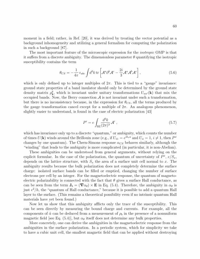
60

moment in a field; rather, in Ref. [20], it was derived by treating the vector potential as abackground inhomogeneity and utilizing a general formalism for computing the polarizationin such a background [87].

The most important feature of the microscopic expression for the isotropic OMP is thatit suffers from a discrete ambiguity. The dimensionless parameter θ quantifying the isotropicsusceptibility contains the term

θCS = − 1

4πεabc

∫d3k tr

[Aa∂bAc − 2i

3AaAbAc

], (5.6)

which is only defined up to integer multiples of 2π. This is tied to a “gauge” invariance:ground state properties of a band insulator should only be determined by the ground statedensity matrix ρgk, which is invariant under unitary transformations Unn′(k) that mix theoccupied bands. Now, the Berry connection A is not invariant under such a transformation,but there is no inconsistency because, in the expression for θCS, all the terms produced bythe gauge transformation cancel except for a multiple of 2π. An analogous phenomenon,slightly easier to understand, is found in the case of electric polarization [43]

P i = e

∫BZ

d3k

(2π)3Ai , (5.7)

which has invariance only up to a discrete “quantum,” or ambiguity, which counts the numberof times U(k) winds around the Brillouin zone (e.g., if U11 = eikxa and Uii = 1, i 6= 1, then P x

changes by one quantum). The Chern-Simons response αCS behaves similarly, although the“winding” that leads to the ambiguity is more complicated (in particular, it is non-Abelian).

These ambiguities can be understood from general arguments, without relying on theexplicit formulae. In the case of the polarization, the quantum of uncertainty of P x, e/Sx,depends on the lattice structure, with Sx the area of a surface unit cell normal to x. Theambiguity results because the bulk polarization does not completely determine the surfacecharge: isolated surface bands can be filled or emptied, changing the number of surfaceelectrons per cell by an integer. For the magnetoelectric response, the quantum of magneto-electric polarizability is connected with the fact that θ gives a surface Hall conductance, ascan be seen from the term Jb = (∇αθ) × E in Eq. (5.4). Therefore, the ambiguity in αθ isjust e2/h, the “quantum of Hall conductance,” because it is possible to add a quantum Halllayer to the surface. (This remains a theoretical possibility even if no intrinsic quantum Hallmaterials have yet been found.)

Now let us show that this ambiguity afflicts only the trace of the susceptibility. Thiscan be seen directly by measuring the bound charge and currents. For example, all thecomponents of α can be deduced from a measurement of ρb in the presence of a nonuniformmagnetic field [see Eq. (5.4)], but αθ itself does not determine any bulk properties.

More concretely, one can derive the ambiguities in the magnetoelectric response from theambiguities in the surface polarization. In a periodic system, which for simplicity we taketo have a cubic unit cell, the smallest magnetic field that can be applied without destroying

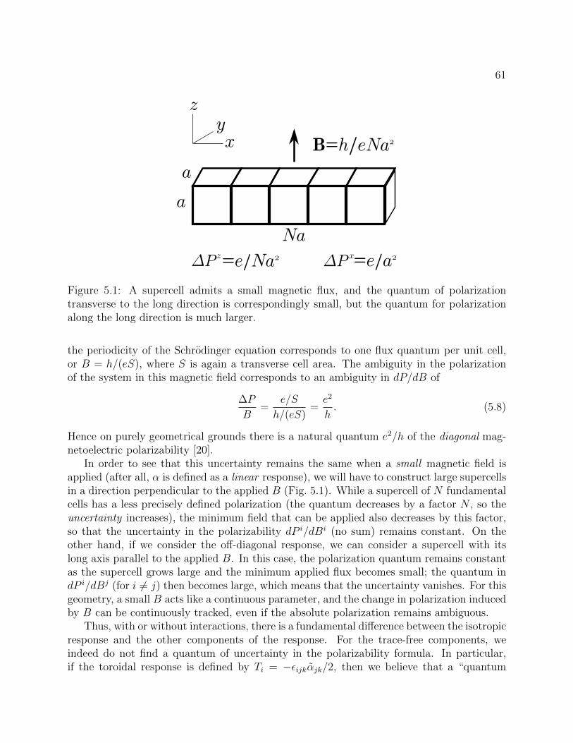
61

Figure 5.1: A supercell admits a small magnetic flux, and the quantum of polarizationtransverse to the long direction is correspondingly small, but the quantum for polarizationalong the long direction is much larger.

the periodicity of the Schrodinger equation corresponds to one flux quantum per unit cell,or B = h/(eS), where S is again a transverse cell area. The ambiguity in the polarizationof the system in this magnetic field corresponds to an ambiguity in dP/dB of

∆P

B=

e/S

h/(eS)=e2

h. (5.8)

Hence on purely geometrical grounds there is a natural quantum e2/h of the diagonal mag-netoelectric polarizability [20].

In order to see that this uncertainty remains the same when a small magnetic field isapplied (after all, α is defined as a linear response), we will have to construct large supercellsin a direction perpendicular to the applied B (Fig. 5.1). While a supercell of N fundamentalcells has a less precisely defined polarization (the quantum decreases by a factor N , so theuncertainty increases), the minimum field that can be applied also decreases by this factor,so that the uncertainty in the polarizability dP i/dBi (no sum) remains constant. On theother hand, if we consider the off-diagonal response, we can consider a supercell with itslong axis parallel to the applied B. In this case, the polarization quantum remains constantas the supercell grows large and the minimum applied flux becomes small; the quantum indP i/dBj (for i 6= j) then becomes large, which means that the uncertainty vanishes. For thisgeometry, a small B acts like a continuous parameter, and the change in polarization inducedby B can be continuously tracked, even if the absolute polarization remains ambiguous.

Thus, with or without interactions, there is a fundamental difference between the isotropicresponse and the other components of the response. For the trace-free components, weindeed do not find a quantum of uncertainty in the polarizability formula. In particular,if the toroidal response is defined by Ti = −εijkαjk/2, then we believe that a “quantum

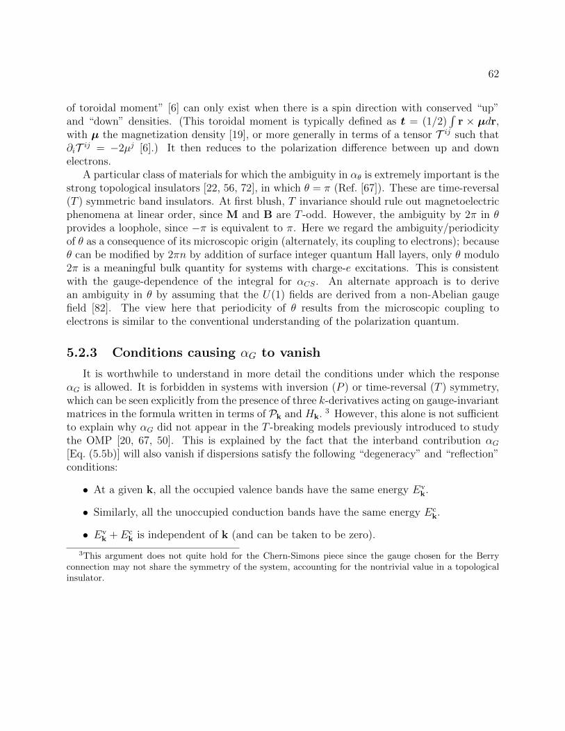
62

of toroidal moment” [6] can only exist when there is a spin direction with conserved “up”and “down” densities. (This toroidal moment is typically defined as t = (1/2)

∫r × µdr,

with µ the magnetization density [19], or more generally in terms of a tensor T ij such that∂iT ij = −2µj [6].) It then reduces to the polarization difference between up and downelectrons.

A particular class of materials for which the ambiguity in αθ is extremely important is thestrong topological insulators [22, 56, 72], in which θ = π (Ref. [67]). These are time-reversal(T ) symmetric band insulators. At first blush, T invariance should rule out magnetoelectricphenomena at linear order, since M and B are T -odd. However, the ambiguity by 2π in θprovides a loophole, since −π is equivalent to π. Here we regard the ambiguity/periodicityof θ as a consequence of its microscopic origin (alternately, its coupling to electrons); becauseθ can be modified by 2πn by addition of surface integer quantum Hall layers, only θ modulo2π is a meaningful bulk quantity for systems with charge-e excitations. This is consistentwith the gauge-dependence of the integral for αCS. An alternate approach is to derivean ambiguity in θ by assuming that the U(1) fields are derived from a non-Abelian gaugefield [82]. The view here that periodicity of θ results from the microscopic coupling toelectrons is similar to the conventional understanding of the polarization quantum.

5.2.3 Conditions causing αG to vanish

It is worthwhile to understand in more detail the conditions under which the responseαG is allowed. It is forbidden in systems with inversion (P ) or time-reversal (T ) symmetry,which can be seen explicitly from the presence of three k-derivatives acting on gauge-invariantmatrices in the formula written in terms of Pk and Hk. 3 However, this alone is not sufficientto explain why αG did not appear in the T -breaking models previously introduced to studythe OMP [20, 67, 50]. This is explained by the fact that the interband contribution αG[Eq. (5.5b)] will also vanish if dispersions satisfy the following “degeneracy” and “reflection”conditions:

• At a given k, all the occupied valence bands have the same energy Evk.

• Similarly, all the unoccupied conduction bands have the same energy Eck.

• Evk + Ec

k is independent of k (and can be taken to be zero).

3This argument does not quite hold for the Chern-Simons piece since the gauge chosen for the Berryconnection may not share the symmetry of the system, accounting for the nontrivial value in a topologicalinsulator.

63

E

k

µ

Figure 5.2: Schematic band structure that leads to vanishing αG. The bands below the chem-ical potential are degenerate with energy Ev

k, while the bands above the chemical potentialhave energy Ec

k = const.− Evk.

This can be seen immediately in an expanded form of the integrand of αG, [see Eqs. (B.11c)and (B.11d)]

−∑

n,n′ occm unocc

(En−En′)〈∂bn|n′〉〈∂an′|m〉〈m|∂in〉

En − Em+

∑n occ

m,m′ unocc

(Em−Em′)〈∂bn|m′〉〈m′|∂am〉〈m|∂in〉

En − Em

−∑n occ

m unocc

∂b(En + Em)〈∂an|m〉〈m|∂in〉

En − Em, (5.9)

where |n〉 = |unk〉 and En = Enk, etc. Such a structure is automatic when only two orbitals(with both spin states) are taken into account and the system has particle-hole and PTsymmetries. PT symmetry guarantees that the bands remain spin-degenerate even if spinis not a good quantum number. To see this, recall that T acts on wave functions as iσyKand maps k → −k. Here, K is complex conjugation and σy takes the form of the usualPauli matrix in the z basis of spin. Then P maps k → −k again, so that PT effectivelyacts as “T at each k” [3] . Then particle-hole symmetry implies that the dispersion isreflection-symmetric, Ev

k = −Eck.

Most model Hamiltonians discussed in the literature that access the topological insulatorphase [22, 67, 20, 36, 50], as well as the Dirac Hamiltonian (in the context of which the axionelectrodynamics was first discussed [82]), can be defined in terms of a Clifford algebra,4

and this ensures that the dispersions are degenerate and reflection symmetric. The onlyexception of which we are aware is the model of Guo and Franz on the pyrochlore lattice,

4Concretely, the generators of a Clifford algebra are a set of Nc matrices Γa that satisfy the relationΓa,Γb = 2δab. Then the Hamiltonians cited take the form H(k) =

∑Nc

a=1 εa(k)Γa. This automatically

satisfies the degeneracy and dispersion-reflection properties, since H(k)’s eigenvalues are ±√∑

a εa(k)2.

64

which has four orbitals per unit cell [28]. The topological insulator phase itself will not havea contribution from αG, since it is T -invariant, and so the Guo and Franz model will notshow such a response; however, the addition of any T -breaking perturbation to their modelshould produce off-diagonal magnetoelectric responses.

Finally, there is a simple mathematical condition that will cause αG to vanish. Namely,αG decreases as the gap becomes large without changing the wave functions, and in the limitof infinite bulk gap the only magnetoelectric response comes from the Chern-Simons part,which is not sensitive to the energies and depends only on the electron wave functions.

5.2.4 Is the Chern-Simons contribution physically distinct?

Apart from the ambiguity in αCS that is not present in αG, there seems to be no realphysical distinction between the two terms of the linear magnetoelectric response. We discusstwo aspects that relate to this observation below.

Localized vs. itinerant contributionsThe ambiguity in θCS can be interpreted as a manifestation of the fact that bulk quantities

cannot determine the surface quantum Hall conductance, since a two-dimensional quantumHall layer could appear on a surface independent of bulk properties. This suggests, perhaps,that the Chern-Simons term appears only in bulk systems with extended wave functions, andis a consequence of the itinerant electrons, while αG is a localized molecule-like contribution.However, this turns out not to be the case.

Consider a periodic array of isolated molecules, which is an extreme limit of the class ofcrystalline insulators. Such a system has flat bands, with energies equal to the energies of themolecular states, since the electrons cannot propagate. It is certainly possible to constructa molecular system where all the unoccupied states have one energy and all the occupiedstates have another, by tuning the potentials. In this case αG will vanish. However, sucha molecule can still display a magnetoelectric response; it will therefore have to be givenby αCS (and so restricted to diagonal responses). For example, consider the “molecule” ofFig. (5.3) with the shape of a regular tetrahedron. If the two low-energy levels are occupied,the magnetoelectric response is

∂P i

∂Bj= ±δij

1√6

e2

,

where P i here is the electric dipole moment divided by the volume of the tetrahedron; thesign of the polarizability reverses when the complex phases are reversed. This shows thatthe Chern-Simons term does not require delocalized orbitals.

AdditivityAnother argument against distinguishing between the Chern-Simons part and the rest of

the susceptibility is based on band additivity. When interactions are not taken into account,each occupied band can be regarded as an independent physical system (at least if there areno band crossings). Applying a magnetic field causes each band n to become polarized by acertain amount Pn, and so the net polarization should be P =

∑n Pn. The Pauli exclusion

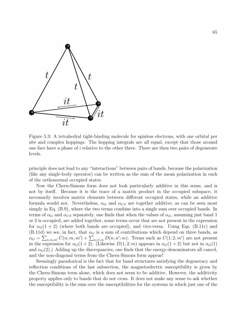
65

it

it

it

tt

t

Figure 5.3: A tetrahedral tight-binding molecule for spinless electrons, with one orbital persite and complex hoppings. The hopping integrals are all equal, except that those aroundone face have a phase of i relative to the other three. There are then two pairs of degeneratelevels.

principle does not lead to any “interactions” between pairs of bands, because the polarization(like any single-body operator) can be written as the sum of the mean polarization in eachof the orthonormal occupied states.

Now the Chern-Simons form does not look particularly additive in this sense, and isnot by itself. Because it is the trace of a matrix product in the occupied subspace, itnecessarily involves matrix elements between different occupied states, while an additiveformula would not. Nevertheless, αG and αCS are together additive, as can be seen mostsimply in Eq. (B.9), where the two terms combine into a single sum over occupied bands. Interms of αG and αCS separately, one finds that when the values of αG, assuming just band 1or 2 is occupied, are added together, some terms occur that are not present in the expressionfor αG(1 + 2) (where both bands are occupied), and vice-versa. Using Eqs. (B.11c) and(B.11d) we see, in fact, that αG is a sum of contributions which depend on three bands, asαG =

∑n,m,m′ C(n;m,m′) +

∑n,n′,mD(n, n′;m). Terms such as C(1; 2,m′) are not present

in the expression for αG(1 + 2). (Likewise D(1, 2;m) appears in αG(1 + 2) but not in αG(1)and αG(2).) Adding up the discrepancies, one finds that the energy-denominators all cancel,and the non-diagonal terms from the Chern-Simons form appear!

Seemingly paradoxical is the fact that for band structures satisfying the degeneracy andreflection conditions of the last subsection, the magnetoelectric susceptibility is given bythe Chern-Simons term alone, which does not seem to be additive. However, the additivityproperty applies only to bands that do not cross. It does not make any sense to ask whetherthe susceptibility is the sum over the susceptibilities for the systems in which just one of the

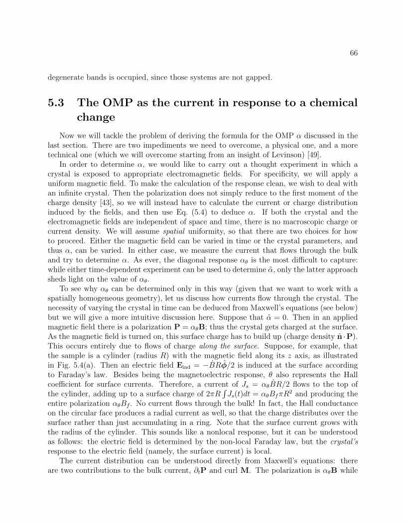
66

degenerate bands is occupied, since those systems are not gapped.

5.3 The OMP as the current in response to a chemical

change

Now we will tackle the problem of deriving the formula for the OMP α discussed in thelast section. There are two impediments we need to overcome, a physical one, and a moretechnical one (which we will overcome starting from an insight of Levinson) [49].

In order to determine α, we would like to carry out a thought experiment in which acrystal is exposed to appropriate electromagnetic fields. For specificity, we will apply auniform magnetic field. To make the calculation of the response clean, we wish to deal withan infinite crystal. Then the polarization does not simply reduce to the first moment of thecharge density [43], so we will instead have to calculate the current or charge distributioninduced by the fields, and then use Eq. (5.4) to deduce α. If both the crystal and theelectromagnetic fields are independent of space and time, there is no macroscopic charge orcurrent density. We will assume spatial uniformity, so that there are two choices for howto proceed. Either the magnetic field can be varied in time or the crystal parameters, andthus α, can be varied. In either case, we measure the current that flows through the bulkand try to determine α. As ever, the diagonal response αθ is the most difficult to capture:while either time-dependent experiment can be used to determine α, only the latter approachsheds light on the value of αθ.

To see why αθ can be determined only in this way (given that we want to work with aspatially homogeneous geometry), let us discuss how currents flow through the crystal. Thenecessity of varying the crystal in time can be deduced from Maxwell’s equations (see below)but we will give a more intuitive discussion here. Suppose that α = 0. Then in an appliedmagnetic field there is a polarization P = αθB; thus the crystal gets charged at the surface.As the magnetic field is turned on, this surface charge has to build up (charge density n ·P).This occurs entirely due to flows of charge along the surface. Suppose, for example, thatthe sample is a cylinder (radius R) with the magnetic field along its z axis, as illustratedin Fig. 5.4(a). Then an electric field Eind = −BRφ/2 is induced at the surface accordingto Faraday’s law. Besides being the magnetoelectric response, θ also represents the Hallcoefficient for surface currents. Therefore, a current of Js = αθBR/2 flows to the top ofthe cylinder, adding up to a surface charge of 2πR

∫Js(t)dt = αθBfπR

2 and producing theentire polarization αθBf . No current flows through the bulk! In fact, the Hall conductanceon the circular face produces a radial current as well, so that the charge distributes over thesurface rather than just accumulating in a ring. Note that the surface current grows withthe radius of the cylinder. This sounds like a nonlocal response, but it can be understoodas follows: the electric field is determined by the non-local Faraday law, but the crystal’sresponse to the electric field (namely, the surface current) is local.

The current distribution can be understood directly from Maxwell’s equations: thereare two contributions to the bulk current, ∂tP and curl M. The polarization is αθB while

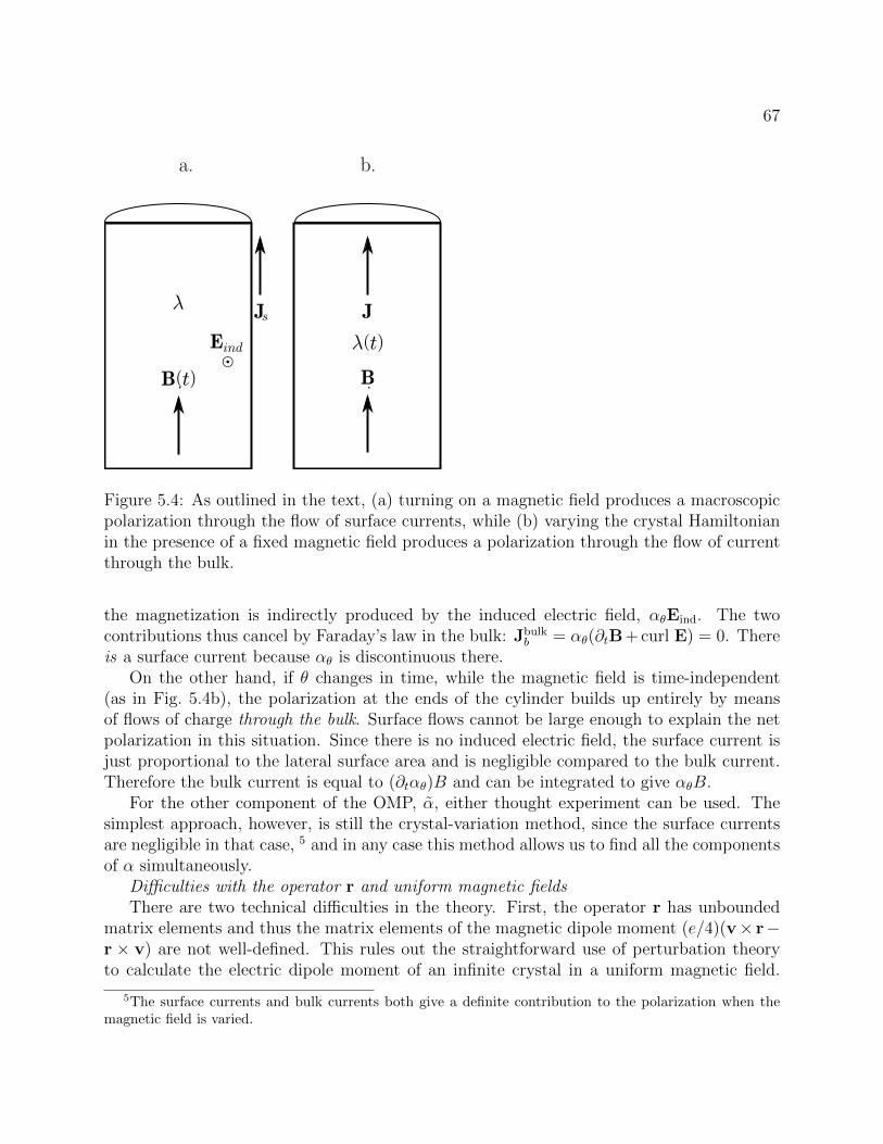
67

Figure 5.4: As outlined in the text, (a) turning on a magnetic field produces a macroscopicpolarization through the flow of surface currents, while (b) varying the crystal Hamiltonianin the presence of a fixed magnetic field produces a polarization through the flow of currentthrough the bulk.

the magnetization is indirectly produced by the induced electric field, αθEind. The twocontributions thus cancel by Faraday’s law in the bulk: Jbulk

b = αθ(∂tB + curl E) = 0. Thereis a surface current because αθ is discontinuous there.

On the other hand, if θ changes in time, while the magnetic field is time-independent(as in Fig. 5.4b), the polarization at the ends of the cylinder builds up entirely by meansof flows of charge through the bulk. Surface flows cannot be large enough to explain the netpolarization in this situation. Since there is no induced electric field, the surface current isjust proportional to the lateral surface area and is negligible compared to the bulk current.Therefore the bulk current is equal to (∂tαθ)B and can be integrated to give αθB.

For the other component of the OMP, α, either thought experiment can be used. Thesimplest approach, however, is still the crystal-variation method, since the surface currentsare negligible in that case, 5 and in any case this method allows us to find all the componentsof α simultaneously.

Difficulties with the operator r and uniform magnetic fieldsThere are two technical difficulties in the theory. First, the operator r has unbounded

matrix elements and thus the matrix elements of the magnetic dipole moment (e/4)(v× r−r × v) are not well-defined. This rules out the straightforward use of perturbation theoryto calculate the electric dipole moment of an infinite crystal in a uniform magnetic field.

5The surface currents and bulk currents both give a definite contribution to the polarization when themagnetic field is varied.

68

Second, if we consider a crystal in a uniform magnetic field, Bloch’s theorem does not hold.Although the magnetic field is uniform, the vector potential that appears in the Hamiltoniandepends on r.

We avoid the problems of r as follows. The key idea is to work with the ground statedensity matrix, rather than wave functions. The individual eigenstates change drasticallywhen a magnetic field, no matter how small, is applied (consider the difference betweena plane wave and a localized Landau level). However, the density matrix of an insulatorsummed over the occupied bands only changes by a small amount when B is applied; overshort distances the magnetic field cannot have a strong effect (even in the example of Lan-dau levels), and the density matrix has only short-range correlations because it describes aninsulating state. More technically, we show (subsection 5.3.1) that the broken translationinvariance of any single-body operator O (such as the density matrix) can be dealt with byfactoring out an Aharonov-Bohm-like phase from its matrix Or1r2 . This solves the problemof the nonuniform gauge field and leads to expressions that depend only on differences be-tween r’s. In addition, since the exponentially decaying ground-state density matrix appearsmultiplying every expression, the factors of r1 − r2 are suppressed.

The calculation then proceeds as follows. First, using the symmetries of the electronHamiltonian in a uniform magnetic field, we find how the density matrix changes in a weakmagnetic field. Next we compute the current response to an adiabatic variation of the crystalHamiltonian. Finally, we show that this current can be expressed as a total time derivative,and therefore can be integrated to give the polarization; at linear order in B we can read offthe coefficients, the magnetoelectric tensor α.

5.3.1 Single-body operators for a uniform magnetic field

Recall the form of the Schrodinger Hamiltonian for a single electron in a crystal andunder the influence of a magnetic field,

HS(p, r) =1

2m[p− eA(r)]2 + V (r), (5.10)

where V (r + R) = V (r) for lattice vectors R. The necessity of using the vector potentialA seems at first to spoil the lattice translation symmetry one would expect in a uniformmagnetic field. However, as noted by Brown [10] and Zak [93], a more subtle form oftranslation symmetry remains. In particular, choosing the gauge

A =1

2B× r, (5.11)

the Hamiltonian has “magnetic translation symmetry”:

HS(p, r + R) = eieB·(R×r)/2HS(p, r)e−ieB·(R×r)/2. (5.12)

This condition defines magnetic translation symmetry for general single-body operators.Any operator O possessing this symmetry can be written in the position basis as

Or1r2 = Or1r2e−ieB·(r1×r2)/2, (5.13a)

69

where O has lattice translation invariance,

Or1+R,r2+R = Or1r2 . (5.13b)

Note that the phase is just (ie/)∫d` ·A calculated along the straight line from r2 to r1,

which agrees with the intuition that comes from writing the second-quantized form of theoperator,

O =

∫d3r1d

3r2 Or1r2c†r1e−ieB·(r1×r2)/2cr2 . (5.14)

This argument shows how to couple general Hamiltonians to uniform fields:

H = exp[(ie/~)

∫ r1

r2

d` ·A][H0r1r2 +H ′r1r2(B)].

The vector potential appears explicitly only in A, while H ′(B) gives the rest of the depen-dence on the magnetic field. The Schrodinger Hamiltonian (5.10) is obtained if we take

H0,r1r2 =

[− 2

2m∇2

r2+ V (r2)

]δ(3)(r2 − r1). (5.15)

and set H ′ = 0. Our results also apply to tight-binding models. We introduce H ′ to capturethe possibility that in a tight-binding model the hoppings will not be rectilinear, and hencethat the phases in Eq. (5.14) do not capture the full field dependence of the Hamiltonian.

5.3.2 The ground state density operator

We find it convenient to work with the one-body density matrix ρg, or equivalently theprojector onto the occupied states, whenever possible, because it is a basis-independentobject. Also, in an insulator, ρgr1r2

is exponentially suppressed in the distance |r2 − r1|,which tempers the divergences that arise from the unboundedness of r [45]. In any case, ifthe ground state is translationally symmetric, the structure described above will apply to ρgand we can be sure that the density matrix has translational symmetry apart from a phase:

ρgr1r2= ρgr1r2

e−ieB·(r1×r2)/2, (5.16)

where ρg possesses the translation symmetry of the crystal lattice and hence should connectsmoothly to the field-free density matrix. Hence we will write

ρg = ρ0 + ρ′, (5.17)

where ρ0 is the density operator of the crystal in the absence of theDensity matrix perturbation theory: Now we have to calculate ρ′, using a kind of pertur-

bation theory that focuses on density matrices rather than wave functions, since the wave-functions suffer from the problems discussed above. This perturbation theory starts from

70

two characteristic properties of the density matrix: it commutes with H, and for fermionsat zero temperature it is a projection operator. The latter means that all states are eitheroccupied or unoccupied, so the eigenvalues of the density operator are 0 and 1, which isformalized as

ρgρg = ρg (5.18)

(idempotency) [17]. Expressed in the position basis,

ρgr1r3=

∫dr2ρ

gr1r2

ρgr2r3

ρgr1r3=

∫dr2ρ

gr1r2

ρgr2r3e−(ie/2)B·(r1×r2+r2×r3+r3×r1). (5.19)

The exponent is just −iφ123/φ0, proportional to the magnetic flux through triangle 123, andthe exponential can be expanded for small B. At first order this gives

ρ′r1r3=

∫dr2[ρ

′r1r2

ρ0r2r3 + ρ0r1r2ρ′r2r3− ρ0r1r2ρ0r2r3 (iφ123/φ0)]. (5.20)

The problem of the unbounded r’s is resolved in this equation because the area A123 of thetriangle is finite and independent of the origin, and also suppressed by the factor of ρ.

Calculation of ρ′: In the last term of Eq. (5.20), we can rewrite 2A123 = r1 × r2 + r2 ×r3 + r3 × r1 = (r2 − r1)× (r3 − r2) and then use (r2 − r1)ρ0r1r2 = [ρ0, r]r1r2 , etc., to obtain

(1− ρ0)ρ′(1− ρ0)− ρ0ρ′ρ0 = −i e2

B · ([ρ0, r]× [ρ0, r]). (5.21)

If we defineH = H0 +H ′, (5.22)

then analogous manipulations (including (r1−r2)Hr1r2 = ivr1r2) on the equation [H, ρg] = 0give

[ρ′, H0] =e

2B · ([ρ0, r]× v − v × [ρ0, r])− [ρ0, H

′]. (5.23)

Eqs. (5.21) and (5.23) have an intuitive meaning. The former equation determines the“interior” matrix elements of ρ′, those between two occupied or two unoccupied states ofthe zero-field Hamiltonian. A perturbation with the full crystal symmetry does not changethe interior matrix elements of the density matrix because of the exclusion principle [53]. Inour case, however, multiplying ρ0 by the phase e(ie/2)B·r1×r2 gives a density matrix with thecorrect magnetic translation symmetry, but also changes the momentum of the states andso results in a small probability for states to be douby occupied. Therefore ρ′ must correctfor this “violation of the exclusion principle.” On the other hand Eq. (5.23) determines the“cross-gap” matrix elements of ρ′ (those between unoccupied and occupied states). Thesematrix elements capture the expected “transitions across the gap” induced by the field. Therest of this section is devoted to calculating all these matrix elements. The results are givenin Eqs. (5.24) and (5.28); the derivations could be skipped on a first reading.

71

Calculation of ρ′. Precisely speaking, Eq. (5.21) gives the matrix elements of ρg betweenpairs of occupied (n and n′) or unoccupied (m and m′) states:

〈ψnk|ρg|ψn′k〉 = δnn′ − e

4BjεjabFabnn′(k)

〈ψmk|(1− ρg)|ψm′k〉 = δmm′ − e

4BjεjabFabmm′(k), (5.24)

where F is the non-Abelian Berry curvature associated with the occupied bands,

Fabnn′ = i〈unk|∂aPk∂bPk − ∂bPk∂

aPk|un′k〉= ∂aAbnn′ − ∂bAann′ − i[Aa,Ab]nn′ , (5.25)

and F is the corresponding quantity for the unoccupied bands. To derive these relations, weuse

ρg =

∫BZ

d3k

(2π)3eik·rPke

−ik·r (5.26)

where P =∑

n occ |unk〉〈unk| is the projector onto filled bands at k. This gives

i[ρg, r] =

∫BZ

d3k

(2π)3eik·r(∇kPk)e−ik·r

=

∫BZ

d3k

(2π)3eik·r 6 rke

−ik·r (5.27)

after discarding a total derivative. The notation 6r = ∇kP was introduced in Eq. (5.5).By contrast, Eq. (5.23) describes to what extent ρg fails to commute with H0, the crystal

Hamiltonian, and gives the matrix elements of ρ′ between occupied and unoccupied states. Inthis sense it is analogous to the more usual results for density-matrix perturbation theory [53].In the basis of unperturbed energy eigenstates,

〈ψnk|ρ′|ψmk〉 = ie

2Bjεjab

〈unk|∂aPk, ∂bHk|umk〉

Enk − Emk

+〈unk|H ′k|umk〉Enk − Emk

. (5.28)

Recall that vb = ∂bHk and that H ′ is introduced only to capture unusual situations such astight-binding models with non-straight hoppings, and vanishes for the continuum problem.Eqs. (5.24) and (5.28) are the key technical results of this formalism, good to linear order inthe magnetic field.

5.3.3 Adiabatic current

Now we need to calculate the current as the Hamiltonian is changed slowly as a function oftime, as in the ordinary theory of polarization [70, 43]. We have to be careful, however, sincethe current vanishes in the zero-order adiabatic ground state described by density matrixρg(t). It is necessary to go to first order in adiabatic perturbation theory, which takes

72

account of the fact that the true dynamical density matrix ρ(t) has an extra contributionproportional to dH/dt = H. However, once the current has been expressed in terms ofρ, which is proportional to H, the distinction is no longer important and the adiabaticapproximation can be made.

Preparing for the adiabatic approximation: We can write the current as

J(t) =e

ΩTrρ(t)v =

e

Ω

i

Trρ[H, r] (5.29)

where Ω is the crystal volume. Here H is the full Hamiltonian including the magneticfield. By unitarity of time evolution, it remains a projector if the initial state describesfilled bands only. The operator r appears here, but in a commutator. Since 〈r1|[O, r]|r2〉 =(r2 − r1)Or1r2 , such expressions do not suffer from the difficulties of an “unprotected” r,namely its unboundedness. We can only use cyclicity of the trace to the extent that thisproperty can be preserved. In particular, the expression Tr r[ρ,H], which seems formallyequivalent to Eq. (5.29), poses problems, but

J(t) =e

Ω

i

Tr[ρ, [ρ, r]][ρ,H] (5.30)

does not. This expression can be derived from Eq. (5.29) using again the idempotency of ρ(ρρ = ρ). Using the equation of motion for the density matrix,

i~ρ(t) = [H(t), ρ(t)], (5.31)

and making the approximation ρ ≈ ρg on the right-hand side at this stage, the currentbecomes

J =e

Ω

∫dr1dr2dr3(r1 − 2r2 + r3)ρ

gr1r2

ρgr2r3ρgr3r1

. (5.32)

Magnetic field dependence of the current : The considerations given in the last subsectionmake the integrand

ρgr1r2ρgr2r3

ρgr3r1= ρgr1r2

ρgr2r3˙ρgr3r1

e−iφ123/φ0 , (5.33)

where, again, φ123 = B ·(r1×r2+r2×r3+r3×r1)/2 is the magnetic flux through the trianglewith vertices r1r2r3 and does not suffer from the pathologies of r itself, which allows us toexpand e−iφ123/φ0 = 1− iφ123/φ0 to lowest order in B (recall again that the matrix elementsof ρ are exponentially suppressed with distances).

Recalling our division ρg = ρ0+ρ′ where ρ′ is of first order in the magnetic field, Eq. (5.32)becomes

J =e

Ω

∫dr1dr2dr3(r1 − 2r2 + r3)

[ρ0r1r2ρ0r2r3 ρ

′r3r1

+ ρ′r1r2ρ0r2r3 ρ0r3r1

+ ρ0r1r2ρ′r2r3

ρ0r3r1 − iφ123

φ0

ρ0r1r2ρ0r2r3 ρ0r3r1

](5.34)

73

at first order. The rest of the calculation involves substituting the expressions for themagnetic-field dependence of ρg obtained earlier, and integrating the result to obtain α.The energy-dependent part of α, namely αG, will come from the mixing of the occupiedand unoccupied bands, Eq. (5.28). The Chern-Simons term will come from the “exclusion-principle–correcting” terms, Eq. (5.24), as well as the φ123 term in the previous equation.

Integrating the results : The four terms in the current can be collected and rearrangedinto the form

J = JG + JCS1 + JCS2 (5.35a)

and integrated with respect to time as follows. The first term can be rewritten with

ρ0r1r2ρ0r2r3 ρ′r3r1

= ∂t(ρ0r1r2ρ0r2r3ρ′r3r1

)− ρ0r1r2ρ0r2r3ρ′r3r1− ρ0r1r2 ρ0r2r3ρ

′r3r1

and combined with the next two terms to give

JG =e

Ω∂tTr[ρ0, r][ρ′, ρ0] (5.35b)

and

JCS1 = −3e

ΩTrρ′[ρ0, [ρ0, r]], (5.35c)

while the final term in Eq. (5.34) (i.e., the term involving φ123) becomes

JCS2 = −i e2

2ΩBjεjabTr[ρ0, r][ρ0, r

a][rb, ρ0] + c.c. (5.35d)

upon rewriting

(r1 − 2r2 + r3)(r1 × r2 + r2 × r3 + r3 × r1)

= (r1 − r2)[(r1 − r3)× (r2 − r3)] + (r3 − r2)[(r1 − r2)× (r1 − r3)].

The total derivative term JG [Eq. (5.35b)] can be written

J iG = ∂t(αG)ijBj (5.36)

with αG as given in Eq. (5.5b),

(αG)ij =e2

Re

∑n occ

m unocc

∫BZ

d3k

(2π)3〈un|∂iP|um〉〈um|εjab∂aH, ∂bP|un〉

En − Em

+ 2e Im∑n occ

m unocc

∫BZ

d3k

(2π)3〈un|∂iP|um〉〈um|∂H ′/∂Bj|un〉

En − Em, (5.37)

where the dependence on k has been suppressed. This result follows immediately upon takingthe trace in the basis of energy eigenstates. Matrix elements of [ρ0, r

i] appear as 6rik = ∂iPk,

74

from Eq. (5.27), and the cross-gap matrix elements of ρ′ in are given in Eq. (5.28). Notethat since JG is a total time derivative, αG is uniquely defined for a given Hamiltonian (thisassumes the existence of a reference Hamiltonian with αG = 0, that is, the existence of atopologically trivial, time-reversal-invariant band insulator).

In JCS2 [Eq. (5.35d)], we can replace r → [[r, ρ0], ρ0] in the third commutator. This hasthe same cross-gap matrix elements as r; the interior matrix elements do not contributeto the trace because the other three factors, ρ0 and two components of [ρ0, r

i], have onlycross-gap matrix elements. Then

JCS2 = ie2

2ΩBjεjabTr[ρ0, r][ρ0, r

a][[[ρ0, rb], ρ0], ρ0] + c.c.

or

JCS2 = − e2

2BjεjabTr∇kPk∂

aPk[[∂bPk,Pk], Pk] + c.c.,

where an integral over k is suppressed for brevity and the trace is taken in the Hilbert spaceat k. Dropping the subscripts k everywhere, this can be expanded and rearranged to give

JCS2 =e2

2BjεjabTrP[∇P , P ]∂aP∂bP + 2[P , ∂bP ][∇P , ∂aP ]

+ 3(P∂bP∂aP∇P + ∂bPP∇P∂aP). (5.35d’)

In manipulating these strings of projection operators and their derivatives, it is very usefulto realize that derivatives of projectors only have cross-gap matrix elements: P∂aPP =Q∂aPQ = 0, where Q = 1 − P is the projector onto unoccupied bands. This means, forexample, that P(∇P)(P) = P(∇P)Q(P)P .

To JCS2 we must add JCS1 [Eq. (5.35c)],

JCS1 =3e2

2BjεjabTr(P −Q)[P ,∇P ]∂aP∂bP

=3e2

2BjεjabTrP[P ,∇P ]∂aP∂bP − (P∂bP∂aP∇P + ∂bPP∇P∂aP), (5.35c’)

to get

JCS = JCS1 + JCS2

=e2

BjεjabTrP[P ,∇P ]∂aP∂bP + [P , ∂bP ][∇P , ∂aP ]. (5.38)

By checking the different components explicitly one can see that this is

JCS = Be2

TrP[P , ∂xP ][∂yP , ∂zP ] + [P , ∂yP ][∂zP , ∂xP ] + [P , ∂zP ][∂xP , ∂yP ], (5.39)

so we get the “topological current”

JCS = −Be2

∫BZ

d3k

(2π)3tr(F txFyz + F tyF zx + F tzFxy), (5.40)

75

where the lower-case trace (tr) is only over the occupied bands, and the Brillouin-zoneintegral has been restored.

It remains only to show that JCS is a total time derivative that integrates to αCSB.Allowing the indices to run over t, x, y, z, in that order (so that εtxyz = +1),

JCS = −Be2

8

∫BZ

d3k

(2π)3εabcdtrFabF cd

= −Be2

2εabcd

∫BZ

d3k

(2π)3∂atr

(Ab∂cAd − i2

3AbAcAd

). (5.41)

The derivatives with respect to kx, ky, kz will vanish when integrated over the Brillouin zoneassuming that A is defined smoothly and periodically over the zone, leaving just

JCS =−Be2

2∂t

∫BZ

d3k

(2π)3εabctr

(Aa∂bAc − i2

3AaAbAc

), (5.42)

where the indices now only run over xyz, as originally. This obviously gives αCS as inEq. (5.5c), completing the proof. It must be reiterated that this integral is not alwaysentirely trivial. In particular, if the adiabatic evolution brings the crystal back to its initialHamiltonian in a nontrivial way, the Brillouin zone integral need not return to its initialvalue because A is not uniquely defined. In other words,

∫dtJCS can be multivalued as a

function of the Hamiltonian deformation parameters. However, the change can only be suchthat θ changes by an integer multiple of 2π, as discussed in subsection 5.2.2.

5.4 Summary

The theoretical calculation of the magnetoelectric polarizability in insulators presents adifficulty similar to that known well from the theory of polarization; both quantities sufferan inherent ambiguity in the bulk. The magnetoelectric polarizability adds another level ofdifficulty because the vector potential is unbounded and breaks lattice translation symme-try. However, we have developed a formalism that allows us to deal directly with a uniformmagnetic field. In the appendix, we further show that a long-wavelength regularization ofthe vector potential together with a suitable generalization of the polarization (to deal withthe broken crystal symmetry) provides a (relatively) simple, though less rigorous, way tocompute the response function. The final expression for the OMP rederives known resultsfor particular model systems and topological insulators and completes the picture with ad-ditional terms that have a relatively straightforward and intuitive interpretation. We hopethat these results and the method of their derivation will be valuable for future work onmagnetoelectric effects and topological electronic phases.

76

Chapter 6

Conclusion

In the introduction it was claimed that the time-reversal-invariant topological insulatorsconsidered here, as well as the quantum Hall phases of matter, are generically characterizedeither by bulk properties (invariants) or edge properties (like the number of zero crossingsof the edge dispersion). The foregoing chapters have focused almost exclusively on the bulkside of this correspondence in the case of topological insulators. Chapter 3 discussed avariant of the original two-dimensional topological invariant that is stable to disorder awayfrom the clean transition, and that therefore serves to classify disordered (noninteracting,time-reversal-invariant) insulators. Chapters 4 and 5 discussed the magnetoelectric responseproperties of three-dimensional bulk insulators, which again give a topological invariant whentime reversal symmetry T is not broken.

Much of the activity in the field of topological insulators to date, by contrast, has focusedon the edge and surface states, not the bulk properties. This is certainly fair, since the edgescarry low-energy excitations, which frequently dominate physical properties of materialsin the experimental regimes of interest. Indeed, discussions of quantum Hall physics oftenmaintain that the really “physical” characteristic is the chiral edge modes, since these modescarry the current in experimental setups.

However, in that case there are bulk measurements as well, like the low-frequency Faradayrotation, that detect the Hall conductance, so that having the bulk characterization is notirrelevant. Furthermore, as pointed out in Chapters 4 and 5, there is great interest inmaterials with bulk magnetoelectric properties, and so the results derived there may proveto be useful in the not-too-distant future. For example, in unpublished work, Sinisa Coh hasalready used them to compute the (small) orbital contributions to the magnetoelectric effectin the benchmark magnetoelectric Cr2O3. Hopefully a deeper understanding of topologicalinsulators will lead to applications in this area.

Still, the fact that the work presented here excludes the boundaries by constructionmeans that there should be more to the story. First, the presence of gapless surface statespose some difficulties for the derivations and numerics presented in the preceding chapters.Fundamentally, when there are gapless excitations none of the derivations in Chapters 3 or5 are valid, since they utilize the adiabatic theorem, and hence its assumption of a spectral

77

gap. Of course, it is still possible to compute transport properties of gapless systems; thecomputation of the current through an insulator, as here, is actually a rather anomalousactivity. The semiclassical formalism used in Chapter 4, for example, assumes that there is agap but not that the chemical potential is in the gap; and there is a way to apply the Kuboformula to metals, although it is apparently a tricky business. So, it should be possible tocompute the transport for a given metallic surface, but it needs to be said that it will bemessier than the what has been explored here; the dissipationless transport considered herehas a nice rigidity to it, which is lost in a metal.

As a specific example of the issues that can arise when the surfaces are taken into account,consider the following situation. As described in Chapter 4, the surface states of the topo-logical insulator can be “gapped out” by applying a magnetic perturbation at the surface,and the sign of the surface Hall conductance then depends on the details of the perturbation.At an edge between two different signs of surface perturbation there is a change in the Hallconductance of ±e2/h, which means on very general grounds that the edge must carry agapless chiral mode. Does this mean that the magnetoelectric polarizability of a topologicalinsulator is generically not measurable, since one should expect to have such edge modes?Or should there be a some stability to a low density of such edges? It may be possible totreat this case by analogy with the integer quantum Hall effect, where disorder can lead tothe presence of such modes in the bulk as well. However, the more general case, in whichthe surface Dirac modes are not gapped everywhere, may require a more novel treatment.

Another open question stems from the very different approaches taken to the topologicalinvariant in Chapters 4 and 5 as compared to that of Chapter 3. The classification oftopological insulators in Chapter 3 depended on the fact that T 2 = −1 for spin-1/2 particles(electrons), and the three-dimensional invariant built from this two-dimensional invarianttherefore seems to require this as well. This requirement is obscured in the formulation of theinvariant as the k-space Chern-Simons integral, or the noncommutative volume introducedin the Interlude, but it can be seen (at least numerically) that the nontrivial value of theintegral requires the sort of band degeneracy implied by T 2 = −1 (i.e., Kramers degeneracy).Even more strikingly, the crucial object in the derivation of Chapter 5 is the density matrixρ =

∑ |ψ〉〈ψ|. If time reversal is represented by Θ, and Θ2ψ = −ψ, then Θ2ρ(Θ−1)2 = ρ andthe information about the spin-1/2 nature of the electron is apparently lost. On the otherhand, the argument in Chapter 4 implying that T -protected topological insulators exist evenin the presence of electron-electron interactions does not depend at all on the spin of theelectron (i.e., Kramers degeneracy).

It may be that the only way to see the effect of strong spin-orbit coupling in generalis to look at the surface modes. For example, this is how the 3D topological insulator ischaracterized in a recent treatment of disordered, noninteracting insulators [74]. Similarly,a bulk OMP of θ = π should be associated with something like gapless Dirac surface modeseven in strongly interacting systems (recall, however, that the precise Dirac structure is notgeneric in the noninteracting, crystalline case, and so cannot be said to be truly fundamental).

It would be more satisfying to be able to trace the connection between the spin of theelectron (i.e., strong spin-orbit coupling) and the topological nature of the phase from bulk

78

considerations, even in the disordered and interacting cases. How does the requirement ofdegeneracy enter? In this regard, it is interesting to note that surface Hall conductances±e2/2h are consistent with the bulk topological insulator, even in the interacting case; thatis, there seems to be a degeneracy lurking in plain sight. Will the bulk degeneracy dependon the topology of the material, as in the case of the fractional quantum Hall effect? Thatwould be one way to reconcile the apparent discrepancy in the descriptions. In any case, thecomputation of the orbital magnetoelectric polarizability in the fully interacting case standsas an interesting and important open problem in this field.

Other questions involve the coupling of the electrons in topological and magnetoelectricmaterials to fields or perturbations other than the electric and magnetic fields, as well asto the electromagnetic field at higher orders. As an example, the old work on axion elec-trodynamics from particle physics points out that there will be higher order responses (F 4

rather than F 2, where F is the field tensor) suppressed by the electron “mass”, i.e., the bandgap. At first glance, a strong magnetic field would seem to simply break the time-reversalinvariance of the topological insulator and remove the interesting physics associated withthat symmetry; these higher-order terms may indicate that a strong field may reveal otherinteresting, although probably not topological, effects.

This nonzero electric or magnetic field, at least when not too strong, can be seen asa perturbation away from the topological insulator, or more general OMP material. It isnot immediately clear what sorts of perturbations will serve to enhance the magnetoelectricresponse of a material. The construction in Chapter 4, in which a coupling to an anti-ferromagnetic order parameter is added to the topological insulator, allows θ to be tunedcontinuously in that model, but in other cases such a coupling may have no effect at allon θ [55]. The non-Chern-Simons response αG derived in Chapter 5 should generically beenhanced by perturbations that reduce the band gap, but since the Chern-Simons responsedepends crucially on the wave functions, it is not enough to look at the energy spectrum tounderstand the effects of varying the Hamiltonian.

On a similar note, it is interesting to ponder how the magnetoelectric response canactually be varied in the laboratory. After all, the derivation proceeds by assuming thepossibility of such variation, at least in principle. Furthermore, it is constructed by analogywith the derivation of the modern theory of polarization [43], which is modeled in turn on theactual experimental protocol for determining changes in polarization. Finding a way to varythe Hamiltonian is like adding an extra dimension to the space in which the material lives,raising the possibility of effectively “looking in the bulk” without having to pass through thesurface.

Finally, an area that has not been much explored to date is the question of the couplingbetween the electrons and other excitations in these materials. For starters, there is atheoretically intriguing, but hardly relevant experimentally, effect know from old work: amaterial with a nonzero value of θ should have a nontrivial coupling to the gravitational field,i.e., the metric of spacetime [12].1 While this sounds at first blush completely removed from

1While the effect due to coupling to the real gravitational field is highly unlikely to be measurable, it

79

the realm of condensed matter physics, it actually raises an interesting point, since the chargethat couples to gravity is energy, and so the associated current is the energy, or heat, currentin the material. It is know that the electronic properties of topological insulator thin filmscan affect the thermal currents in thin-film geometries [27]. What happens as a result of thecoupling between the electrons and other excitations of the material, say, acoustic phononsor magnons? These are linearly dispersing bosons that couple to the electrons, like photons(and gravitons); it is therefore reasonable to expect that the unusual electronic structurethat generates the magnetoelectric effect (and the “gravitational Hall effect”) should alsogenerate an interesting effect due to this coupling. More generally, orbital magnetoelectricsshould be expected to serve as a background for exciting future developments in condensedmatter physics.

should be noted that there are condensed matter models that have emergent gravitational fields [89], andit would be interesting to try to construct such a model that also had nonzero θ, in which case this effectwould appear.

80

Bibliography

[1] B. L. Altshuler, A. G. Aronov, D. E. Khmel’nitskii, and A. I. Larkin. In I. M. Lifshits,editor, Quantum Theory of Solids. 1982.

[2] B. L. Altshuler, A. G. Aronov, A. I. Larkin, and D. E. Khmel’nitskii. Zh. Eskp. Teor.Fiz., 81:768, 1981. [Sov. Phys. JETP 54, 411 (1981)].

[3] J. E. Avron, L. Sadun, J. Segert, and B. Simon. Topological invariants in fermi systemswith time-reversal invariance. Phys. Rev. Lett., 61(12):1329–1332, Sep 1988.

[4] J. E. Avron, R. Seiler, and B. Simon. Homotopy and quantization in condensed matterphysics. Phys. Rev. Lett., 51(1):51–53, 1983.

[5] Joseph E. Avron and R. Seiler. Quantization of the Hall conductance for general,multiparticle Schr’odinger Hamiltonians. Phys. Rev. Lett., 54(4):259–262, 1985.

[6] C. D. Batista, G. Ortiz, and A. A. Aligia. Ferrotoroidic moment as a quantum geometricphase. Physical Review Letters, 101(7):077203, 2008.

[7] G. Bergmann. Weak anti-localization–an experimental proof for the destructive inter-ference of rotated spin 1/2. Solid State Communications, 42(11):815 – 817, 1982.

[8] B. A. Bernevig, T. L. Hughes, and S.-C. Zhang. Quantum Spin Hall Effect and Topo-logical Phase Transition in HgTe Quantum Wells. Science, 314:1757–, December 2006.

[9] M. V. Berry. Quantal phase-factors accompanying adiabatic changes. Proc. Roy. Soc.A, 392:45–57, 1984.

[10] E. Brown. Bloch electrons in a uniform magnetic field. Phys. Rev., 133(4A):A1038–A1044, Feb 1964.

[11] Yu. A. Bychkov and E. I. Rashba. Properties of a 2d electron gas with lifted spectraldegeneracy. JETP Lett., 39(2):78–81, 1984.

[12] C. G. Callan Jr. and J. A. Harvey. Anomalies and fermion zero modes on strings anddomain walls. Nuclear Physics B, 250(1-4):427 – 436, 1985.

81

[13] J. T. Chalker and P. D. Coddington. Percolation, quantum tunnelling and the integerHall effect. J. Phys. C: Solid State Phys., 21:2665–2679, 1988.

[14] Y. L. Chen, J. G. Analytis, J. H. Chu, Z. K. Liu, S. K. Mo, X. L. Qi, H. J. Zhang, D. H.Lu, X. Dai, Z. Fang, S. C. Zhang, I. R. Fisher, Z. Hussain, and Z.-X. Shen. ExperimentalRealization of a Three-Dimensional Topological Insulator, Bi2Te3. 325:178–181, 2009.

[15] Giulio D’Agostini. Bayesian inference in processing experimental data: Principles andbasic applications. Rept. Prog. Phys., 63:1383–1420, 2003.

[16] C. de Grandi and Anatoli Polkovnikov. Adiabatic perturbation theory: from landau-zener problem to quenching through a quantum critical point. in Quantum Quenching,Annealing and Computation, eds. A. Das, A. Chandra and B. K. Chakrabarti, Lect.Notes in Phys., vol. 802 (Springer, Heidelberg 2010).

[17] P. A. M. Dirac. Note on the interpretation of the density matrix in the many-electron problem. Proc. Cam. Phil. Soc., 27:240–243, 1931. in The collected worksof P. A. M. Dirac, 1924-1928, ed. R. H. Dalitz, Cambridge University Press (1995),p 497.

[18] M. I. D’yakonov and V. I. Perel. Possibility of orienting electron spins with current.JETP Lett., 13:467, 1971.

[19] Claude Ederer and Nicola A. Spaldin. Towards a microscopic theory of toroidal momentsin bulk periodic crystals. Physical Review B, 76(21):214404, 2007.

[20] Andrew M. Essin, Joel E. Moore, and David Vanderbilt. Magnetoelectric polariz-ability and axion electrodynamics in crystalline insulators. Physical Review Letters,102(14):146805, 2009.

[21] M. Fiebig. Revival of the magnetoelectric effect. J. Phys. D - Applied Phys., 38:R123–R152, 2005.

[22] L. Fu, C. L. Kane, and E. J. Mele. Topological insulators in three dimensions. Phys.Rev. Lett., 98:106803, 2007.

[23] Liang Fu and C. L. Kane. Time reversal polarization and a Z2 adiabatic spin pump.Phys. Rev. B, 74:195312, 2006.

[24] Liang Fu and C. L. Kane. Topological insulators with inversion symmetry. Phys. Rev.B, 76:045302, 2007.

[25] T. Fukui and Y. Hatsugai. Quantum spin Hall effect in three dimensional materials:Lattice computation of Z2 topological invariants and its application to Bi and Sb. J.Phys. Soc. Jpn., 76:053702, 2007.

82

[26] Takahiro Fukui and Yasuhiro Hatsugai. Quantum spin Hall effect in three dimensionalmaterials: Lattice computation of Z2 topological invariants and its application to Biand Sb. Phys. Rev. B, 75:121403, 2007.

[27] Pouyan Ghaemi, Roger S. K. Mong, and Joel E. Moore. In-plane transport and enhancedthermoelectric performance in thin films of the topological insulators Bi2Te3 and Bi2Se3.arXiv:1002.1341, 2010.

[28] H.-M. Guo and M. Franz. Three-dimensional topological insulators on the pyrochlorelattice. Physical Review Letters, 103(20):206805, 2009.

[29] F. D. M. Haldane. Model for a quantum Hall effect without Landau levels: Condensed-matter realization of the “parity anomaly”. Physical Review Letters, 61:2015–2018,October 1988.

[30] B. I. Halperin. Quantized Hall conductance, current-carrying edge states, and theexistence of extended states in a two-dimensional disordered potential. Phys. Rev. B,25:2185, 1982.

[31] M. Z. Hasan and C. L. Kane. Topological Insulators. unpublished; arXiv:1002.3895,2010.

[32] F. W. Hehl, Y. N. Obukhov, J.-P. Rivera, and H. Schmid. Relativistic analysis ofmagnetoelectric crystals: Extracting a new 4-dimensional P odd and T odd pseudoscalarfrom Cr2O3 data. Physics Letters A, 372:1141–1146, February 2008.

[33] Shinobu Hikami. Localization, nonlinear σ model, and string theory. Prog. Theor. Phys.Suppl., 107:213–227, 1992.

[34] Shinobu Hikami, Anatoly I. Larkin, and Yosuke Nagaoka. Spin-orbit interaction andmagnetoresistance in the two dimensional random system. Prog. Theor. Phys., 63:707–710, 1980.

[35] R. M. Hornreich and S. Shtrikman. Theory of gyrotropic birefringence. Phys. Rev.,171(3):1065–1074, Jul 1968.

[36] Pavan Hosur, Shinsei Ryu, and Ashwin Vishwanath. Chiral topological insulators,superconductors, and other competing orders in three dimensions. Phys. Rev. B,81:045120, 2010.

[37] D. Hsieh, D. Qian, L. Wray, Y. Xia, Y. S. Hor, R. J. Cava, and M. Z. Hasan. Atopological Dirac insulator in a quantum spin Hall phase. Nature, 452:970, 2008.

[38] Daniel Huertas-Hernando, F. Guinea, and Arne Brataas. Spin-orbit coupling in curvedgraphene, fullerenes, nanotubes, and nanotube caps. Phys. Rev. B, 74(15):155426, Oct2006.

83

[39] C. L. Kane and E. J. Mele. Quantum spin Hall effect in graphene. Phys. Rev. Lett.,95:226801, 2005.

[40] C. L. Kane and E. J. Mele. Z2 topological order and the quantum spin Hall effect. Phys.Rev. Lett., 95:146802, 2005.

[41] Y. K. Kato, R. C. Myers, A. C. Gossard, and D. D. Awschalom. Observation of thespin Hall effect in semiconductors. Science, 306:1910, 2004.

[42] D. E. Khmelnitskii. Quantum hall effect and additional oscillations of conductivity inweak magnetic fields. Physics Letters A, 106(4):182 – 183, 1984.

[43] R. D. King-Smith and David Vanderbilt. Theory of polarization of crystalline solids.Phys. Rev. B, 47(3):1651–1654, Jan 1993.

[44] M. Koenig, S. Wiedmann, C. Bruene, A. Roth, H. Buhmann, L. W. Molenkamp, X.-L.Qi, and S.-C. Zhang. Quantum Spin Hall Insulator State in HgTe Quantum Wells.Science, 318:766, October 2007.

[45] Walter Kohn. Theory of the insulating state. Phys. Rev., 133(1A):A171–A181, Jan1964.

[46] R. B. Laughlin. Quantized Hall conductivity in two dimensions. Phys. Rev. B, 23:5632,1981.

[47] R. B. Laughlin. Levitation of extended-state bands in a strong magnetic field. Phys.Rev. Lett., 52(25):2304, Jun 1984.

[48] S.-S. Lee and S. Ryu. Many-Body Generalization of the Z2 Topological Invariant forthe Quantum Spin Hall Effect. Physical Review Letters, 100(18):186807–+, May 2008.

[49] I. B. Levinson. Zh. Eskp. Teor. Fiz., 57:660, 1970. [Sov. Phys. JETP 30, 362 (1970)].

[50] Rundong Li, Jing Wang, Xiaoliang Qi, and Shou-Cheng Zhang. 2009. arXiv:0908.1537.

[51] Andrei Malashevich, Ivo Souza, Sinisa Coh, and David Vanderbilt. Theory of orbitalmagnetoelectric response. unpublished; arXiv:1002.0300, 2010.

[52] Nicola Marzari and David Vanderbilt. Maximally localized generalized wannier functionsfor composite energy bands. Phys. Rev. B, 56(20):12847–12865, Nov 1997.

[53] R. McWeeny. Perturbation theory for the fock-dirac density matrix. Phys. Rev.,126(3):1028–1034, May 1962.

[54] Hongki Min, J. E. Hill, N. A. Sinitsyn, B. R. Sahu, Leonard Kleinman, and A. H.MacDonald. Intrinsic and rashba spin-orbit interactions in graphene sheets. Phys. Rev.B, 74(16):165310, Oct 2006.

84

[55] Roger S. K. Mong, Andrew M. Essin, and Joel E. Moore. Antiferromagnetic topologicalinsulators. arXiv:1004.1403, 2010.

[56] J. E. Moore and L. Balents. Topological invariants of time-reversal-invariant bandstructures. Phys. Rev. B, 75:121306(R), 2007.

[57] J. E. Moore, Y. Ran, and X.-G. Wen. Topological Surface States in Three-DimensionalMagnetic Insulators. Physical Review Letters, 101(18):186805–+, October 2008.

[58] Joel E. Moore. The birth of topological insulators. Nature, (464):194–198, 2010.

[59] S. Murakami, N. Nagaosa, and S.-C. Zhang. Dissipationless spin current at room tem-perature. Science, 301:1348, 2003.

[60] M. Nakahara. Geometry, Topology and Physics. Institute of Physics, 1998.

[61] Qian Niu and D. J. Thouless. Quantum Hall effect with realistic boundary conditions.Phys. Rev. B, 35(5):2188–2197, 1987.

[62] Qian Niu, D. J. Thouless, and Yong-Shi Wu. Quantized Hall conductance as a topolog-ical invariant. Phys. Rev. B, 31(6):3372–3377, 1985.

[63] Hideaki Obuse, Akira Furusaki, Shinsei Ryu, and Christopher Mudry. Two-dimensionalspin-filtered chiral network modelof the Z2 quantum spin-Hall effect. cond-mat/0702199,2007.

[64] Masaru Onoda, Yshai Avishai, and Naoto Nagaosa. Localization in a quantum spinHall system. Phys. Rev. Lett, 98:076802, 2007.

[65] Gerardo Ortiz and Richard M. Martin. Macroscopic polarization as a geometric quan-tum phase: Many-body formulation. Phys. Rev. B, 49(20):14202–14210, May 1994.

[66] A. M. M. Pruisken. Universal singularities in the integral quantum hall effect. Phys.Rev. Lett., 61(11):1297–1300, Sep 1988.

[67] Xiao-Liang Qi, Taylor L. Hughes, and Shou-Cheng Zhang. Topological field theory oftime-reversal invariant insulators. Physical Review B, 78:195424, 2008.

[68] Xiao-Liang Qi and Shou-Cheng Zhang. The quantum spin hall effect and topologicalinsulators. Physics Today, 63(1):33–38, 2010.

[69] E. I. Rashba, L. E. Zhukov, and A. L. Efros. Orthogonal localized wave functions of anelectron in a magnetic field. Phys. Rev. B, 55:5306–5312, 1997.

[70] R. Resta. Theory of the electric polarization in crystals. Ferroelectrics, 136(1):51, 1992.

85

[71] Rahul Roy. Z2 classification of quantum spin hall systems: An approach using time-reversal invariance. Phys. Rev. B, 79(19):195321, May 2009.

[72] Rahul Roy. Topological phases and the quantum spin hall effect in three dimensions.Phys. Rev. B, 79(19):195322, May 2009.

[73] J. J. Sakurai. Modern Quantum Mechanics, chapter 4.4. Addison-Wesley, 1994.

[74] Andreas P. Schnyder, Shinsei Ryu, Akira Furusaki, and Andreas W. W. Ludwig. Classi-fication of topological insulators and superconductors in three spatial dimensions. Phys.Rev. B, 78:195125, 2008.

[75] D. N. Sheng, Z. Y. Weng, L. Sheng, and F. D. M. Haldane. Quantum spin-hall effectand topologically invariant chern numbers. Phys. Rev. Lett., 97(3):036808, Jul 2006.

[76] Jairo Sinova, Dimitrie Culcer, Q. Niu, N. A. Sinitsyn, T. Jungwirth, and A. H. Mac-Donald. Universal intrinsic spin hall effect. Phys. Rev. Lett., 92(12):126603, Mar 2004.

[77] N. A. Spaldin and M. Fiebig. The renaissance of magnetoelectric multiferroics. Science,309:391–392, 2005.

[78] T. Thonhauser, Davide Ceresoli, David Vanderbilt, and R. Resta. Orbital magnetizationin periodic insulators. Phys. Rev. Lett., 95(13):137205, Sep 2005.

[79] D. J. Thouless. Quantization of particle transport. Phys. Rev. B, 27(10):6083–6087,May 1983.

[80] D. J. Thouless. Wannier functions for magnetic sub-bands. Journal of Physics C: SolidState Physics, 17(12):L325, 1984.

[81] D. J. Thouless, M. Kohmoto, M. P. Nightingale, and M. den Nijs. Quantized HallConductance in a Two-Dimensional Periodic Potential. Phys. Rev. Lett., 49:405, 1982.

[82] F. Wilczek. Two applications of axion electrodynamics. Phys. Rev. Lett., 58:1799, 1987.

[83] Jacek C. Wojde l and Jorge Iniguez. Magnetoelectric response of multiferroic bifeo3 andrelated materials from first-principles calculations. Phys. Rev. Lett., 103:267205, 2009.

[84] J. Wunderlich, B. Kaestner, J. Sinova, and T. Jungwirth. Experimental observationof the spin-hall effect in a two-dimensional spin-orbit coupled semiconductor system.Phys. Rev. Lett., 94(4):047204, Feb 2005.

[85] Y. Xia, D. Qian, D. Hsieh, L. Wray, A. Pal, H. Lin, A. Bansil, D. Grauer, Y. S. Hor,R. J. Cava, and M. Z. Hasan. Observation of a large-gap topological-insulator class witha single Dirac cone on the surface. Nature Physics, 5:398–402, May 2009.

86

[86] Di Xiao, Ming-Che Chang, and Qian Niu. Berry phase effects on electronic properties.arXiv:0907.2021, 2009.

[87] Di Xiao, Junren Shi, Dennis P. Clougherty, and Qian Niu. Polarization and adiabaticpumping in inhomogeneous crystals. Phys. Rev. Lett., 102:087602, 2009.

[88] Di Xiao, Junren Shi, and Qian Niu. Berry phase correction to electron density of statesin solids. Phys. Rev. Lett., 95(13):137204, Sep 2005.

[89] Cenke Xu. Gapless bosonic excitation without symmetry breaking: An algebraic spinliquid with soft gravitons. Phys. Rev. B, 74(22):224433, Dec 2006.

[90] Kun Yang and R. N. Bhatt. Floating of extended states and localization transistion ina weak magnetic field. Phys. Rev. Lett., 76(8):1316–1319, 1996.

[91] W.-M. Yao, C. Amsler, D. Asner, R.M. Barnett, J. Beringer, P.R. Burchat, C.D.Carone, C. Caso, O. Dahl, G. D’Ambrosio, A. DeGouvea, M. Doser, S. Eidelman, J.L.Feng, T. Gherghetta, M. Goodman, C. Grab, D.E. Groom, A. Gurtu, K. Hagiwara,K.G. Hayes, J.J. Hernandez-Rey, K. Hikasa, H. Jawahery, C. Kolda, Kwon Y., M.L.Mangano, A.V. Manohar, A. Masoni, R. Miquel, K. Monig, H. Murayama, K. Naka-mura, S. Navas, K.A. Olive, L. Pape, C. Patrignani, A. Piepke, G. Punzi, G. Raf-felt, J.G. Smith, M. Tanabashi, J. Terning, N.A. Tornqvist, T.G. Trippe, P. Vogel,T. Watari, C.G. Wohl, R.L. Workman, P.A. Zyla, B. Armstrong, G. Harper, V.S. Lu-govsky, P. Schaffner, M. Artuso, K.S. Babu, H.R. Band, E. Barberio, M. Battaglia,H. Bichsel, O. Biebel, P. Bloch, E. Blucher, R.N. Cahn, D. Casper, A. Cattai, A. Cec-cucci, D. Chakraborty, R.S. Chivukula, G. Cowan, T. Damour, T. DeGrand, K. Desler,M.A. Dobbs, M. Drees, A. Edwards, D.A. Edwards, V.D. Elvira, J. Erler, V.V. Ezhela,W. Fetscher, B.D. Fields, B. Foster, D. Froidevaux, T.K. Gaisser, L. Garren, H.-J. Ger-ber, G. Gerbier, L. Gibbons, F.J. Gilman, G.F. Giudice, A.V. Gritsan, M. Grunewald,H.E. Haber, C. Hagmann, I. Hinchliffe, A. Hocker, P. Igo-Kemenes, J.D. Jackson, K.F.Johnson, D. Karlen, B. Kayser, D. Kirkby, S.R. Klein, K. Kleinknecht, I.G. Knowles,R.V. Kowalewski, P. Kreitz, B. Krusche, Yu.V. Kuyanov, O. Lahav, P. Langacker,A. Liddle, Z. Ligeti, T.M. Liss, L. Littenberg, L. Liu, K.S. Lugovsky, S.B. Lugovsky,T. Mannel, D.M. Manley, W.J. Marciano, A.D. Martin, D. Milstead, M. Narain, P. Na-son, Y. Nir, J.A. Peacock, S.A. Prell, A. Quadt, S. Raby, B.N. Ratcliff, E.A. Razuvaev,B. Renk, P. Richardson, S. Roesler, G. Rolandi, M.T. Ronan, L.J. Rosenberg, C.T.Sachrajda, S. Sarkar, M. Schmitt, O. Schneider, D. Scott, T. Sjostrand, G.F. Smoot,P. Sokolsky, S. Spanier, H. Spieler, A. Stahl, T. Stanev, R.E. Streitmatter, T. Sumiyoshi,N.P. Tkachenko, G.H. Trilling, G. Valencia, K. van Bibber, M.G. Vincter, D.R. Ward,B.R. Webber, J.D. Wells, M. Whalley, L. Wolfenstein, J. Womersley, C.L. Woody,A. Yamamoto, O.V. Zenin, J. Zhang, and R.-Y. Zhu. Review of Particle Physics. J.Phys. G, 33:1, 2006. §32.

87

[92] Yugui Yao, Fei Ye, Xiao-Liang Qi, Shou-Cheng Zhang, and Zhong Fang. Spin-orbit gapof graphene: First-principles calculations, Jan 2007.

[93] J. Zak. Magnetic translation group. Phys. Rev., 134(6A):A1602–A1606, Jun 1964.

[94] Paolo Zanardi, Paolo Giorda, and Marco Cozzini. Information-theoretic differentialgeometry of quantum phase transitions. Phys. Rev. Lett., 99(10):100603, Sep 2007.

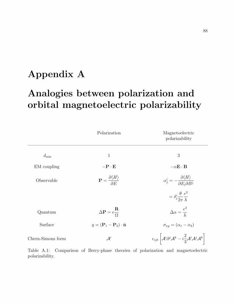
88

Appendix A

Analogies between polarization andorbital magnetoelectric polarizability

Polarization Magnetoelectricpolarizability

dmin 1 3

EM coupling −P · E −αE ·B

Observable P =∂〈H〉∂E

αij = − ∂〈H〉∂Ei∂Bj

= δijθ

2π

e2

h

Quantum ∆P = eR

Ω∆α =

e2

h

Surface q = (P1 −P2) · n σxy = (α1 − α2)

Chern-Simons form Ai εijk

[Ai∂jAk − i2

3AiAjAk

]Table A.1: Comparison of Berry-phase theories of polarization and magnetoelectricpolarizability.

89

Appendix B

Calculating the OMP using staticpolarization

As noted in the text, matrix elements of the operator r are ill-behaved in a basis ofextended, Bloch-like states. That problem was solved by working with the density operatorρ, whose matrix elements are exponentially suppressed with distance. Another approach isto use a Wannier-like basis of localized states. In this appendix, we take this approach topresent an alternative derivation of the OMP.

The Bloch functions ψnk(r) of the unperturbed crystal will evolve, under the applicationof a long-wavelength magnetic field A = A0 sin q · r, into the exact energy eigenfunctionsΨnk(r). These no longer have a sharp crystal momentum k, but may be expanded in aperturbation series in the unperturbed ψnk(r). Then the analogue to the standard Wannierfunction wnR(r) for lattice vector R will be

WnR(r) =Ω√N

∫BZ

d3k

(2π)3Ψnk(r)e−ik·R

= wnR(r) + δwnR(r), (B.1)

where Ω is the volume of the crystal and N is the number of unit cells. The Wannier orbitalscentered at R become polarized when the magnetic field is applied, and this distortion givesa polarization density of

δP(R) =1

Ω

∑n occ

〈wnR|er|δwnR〉+ c.c. (B.2)

Although it is not obvious that the bulk polarization appearing in Maxwell’s equations is thesame as the polarization of a set of Wannier orbitals, this expression leads to Eq. (5.5). To en-sure that the Wannier orbitals are localized, we will have to suppose that each band has a van-ishing Chern number,[80] so that the phase of unk can be chosen so that it is a periodic func-tion of k. In this case the unperturbed Wannier functions are localized, and (though thereare usually subtleties in defining Wannier functions in a magnetic fields),[69] the regulariza-tion used here leads to localized orbitals. Presumably these arguments can be extended to

90

the case where the total Chern number for all occupied bands Cij =∑

n occ

∫BZd3kF ijnn(k)/2π

vanishes.Here we want to take a relatively direct approach to perturbation theory in the field, and

write[88]

Ψnk = ψnk + δψnk (B.3)

δψnk =eB

2iq

∑l

[ψlk+q

〈ulk+q|vx|unk〉Enk − Elk+q + iε

− (q → −q)].

For definiteness we take A = −(B/q) sin(qy)x, and the velocity operator can be alternativelyexpressed as vx = ∂xHk/, with Hk the Bloch Hamiltonian of the unperturbed crystal.

Then the first-order correction to the dipole moment of the generalized Wannier functionswill be

δP i(R) = e∑n occ

∫dr

∫BZ

d3k

(2π)3(rieik·(R−r)u∗nk(r)

) ∫BZ

d3k′

(2π)3δψnk′(r)e−ik

′·R + c.c. (B.4)

The position integral must be taken over the whole crystal at this point. In the integral overk, ri can be converted into a k derivative of the exponential, and then partial integrationleaves a factor −i∂kiu∗ (the boundary term vanishes because the Bloch function ψ is strictlyperiodic in k). Then

δP i = −e2B

2q

∑n occl

[〈∂iunk|ulk〉〈ulk|vx|unk−q〉

Enk−q − Elk + iεeiq·R − (q → −q)

]+ c.c. (B.5)

(From now on, we will omit the integral over k and the associated factor of (2π)3.) Becauseof the variation of the magnetic field the magnetoelectric polarization δP i(R) = αijB

j(R)should vary as cos q ·R. The polarization seems to have both cosine and sine terms, but thecoefficient of the latter is −B sin(qy)Cix/q, and the vanishing of C is a prerequisite for usingWannier functions.

To lowest order in q and B, then, the magnetoelectric response is

αij = −e2

2εjab∂qb

∑l

n occ

〈∂iunk|ulk〉〈ulk|va|unk−q〉Enk−q − Elk + iε

+ c.c., (B.6)

where we have symmetrized over Landau gauges to make the expression nicer.Switching to the shorthand |n〉 = |unk〉,

αij =e2

εjabRe

∑n occl

[〈∂in|l〉〈l|∂aH|∂bn〉En − El + iε

− 〈∂in|l〉〈l|∂aH|n〉∂bEn(En − El + iε)2

]. (B.7)

91

Simplifying the second term of this expression makes use of the “Sternheimer equation”

(∂aH)|n〉 = (En −H)|∂an〉+ (∂aEn)|n〉 (B.8)

and the antisymmetry in the indices a and b to give

αij =e2

2εjab

∑n occl

〈∂in|l〉〈l|∂a(H + En)|∂bn〉En − El + iε

+ c.c. (B.9)

Note the formal similarity to the expression for orbital magnetization,

Mj =1

2Im∑n occ

εjab〈∂an|(H + En)|∂bn〉 = −1

2Im∑n occ

εjab〈n|∂a(H + En)|∂bn〉, (B.10)

in particular the appearance of the combination H + En.[78, 88]To bring our compact expression into the form given in terms of αG and αCS in the

main text, we need to break the sum over l into contributions from occupied and unoccupiedstates. Omitting the factor (e2/2~)εjab for the moment, the sum over the occupied statestakes the form

∑n,locc

〈∂in|l〉〈l|∂a(H + En)|∂bn〉En − El + iε

+ c.c. =∑n,locc

〈∂in|l〉〈l|∂a(H − El)|∂bn〉+ 〈∂bl|∂a(H − En)|n〉

En − El + iε

=∑n,n′occ

〈∂in|n′〉〈∂bn′|∂an〉 (B.11a)

using the antisymmetry in a and b and the Sternheimer equation again. Because the twosums are not symmetric when we take l in the unoccupied space, however, the terms do notcancel as nicely. Inserting a resolution of the identity, broken into two parts, gives:∑

n,n′ occm unocc

〈∂in|m〉〈m|∂aH|n′〉〈n′|∂bn〉En − Em

+ c.c.

=∑

n,n′ occm unocc

〈∂in|m〉〈m|∂an′〉〈n′|∂bn〉+ c.c. (B.11b)

−∑

n,n′ occm unocc

〈∂in|m〉〈m|∂an′〉〈n′|∂bH|n〉En − Em

+ c.c. (B.11c)

+∑n occ

m unocc

〈∂in|m〉〈m|∂an〉∂bEnEn − Em

+ c.c.

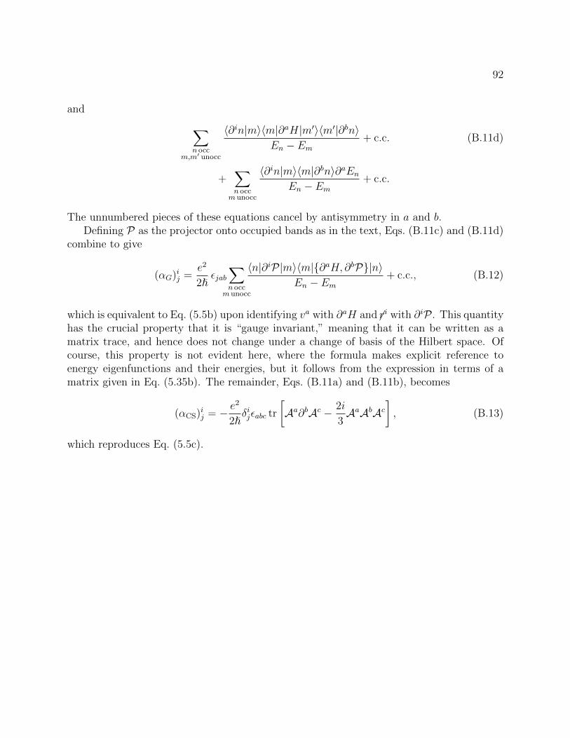
92

and ∑n occ

m,m′ unocc

〈∂in|m〉〈m|∂aH|m′〉〈m′|∂bn〉En − Em

+ c.c. (B.11d)

+∑n occ

munocc

〈∂in|m〉〈m|∂bn〉∂aEnEn − Em

+ c.c.

The unnumbered pieces of these equations cancel by antisymmetry in a and b.Defining P as the projector onto occupied bands as in the text, Eqs. (B.11c) and (B.11d)

combine to give

(αG)ij =e2

2εjab

∑n occ

m unocc

〈n|∂iP|m〉〈m|∂aH, ∂bP|n〉En − Em

+ c.c., (B.12)

which is equivalent to Eq. (5.5b) upon identifying va with ∂aH and 6ri with ∂iP . This quantityhas the crucial property that it is “gauge invariant,” meaning that it can be written as amatrix trace, and hence does not change under a change of basis of the Hilbert space. Ofcourse, this property is not evident here, where the formula makes explicit reference toenergy eigenfunctions and their energies, but it follows from the expression in terms of amatrix given in Eq. (5.35b). The remainder, Eqs. (B.11a) and (B.11b), becomes

(αCS)ij = − e2

2δijεabc tr

[Aa∂bAc − 2i

3AaAbAc

], (B.13)

which reproduces Eq. (5.5c).

Electric and Magnetic Response Properties of...

Documents

Transcript of Electric and Magnetic Response Properties of...