ELECTE S DEC21 C - DTIC
200
"AD-A258 420 AFIT/GSM/LSY/92S-13 DTIc ELECTE S DEC21 1992U C THE THEORY OF CONSTRAINTS APPLIED TO PROJECT SCHEDULING: THE CRITICAL CHAIN CONCEPT DEFINED THESIS Andrew D. Ingram, B.S. Paul E. Scherer, B.S. Capt, USAF Capt, USAF AFIT/GSM/LSY/92S-13 Approved for public release; distribution unlimited 92-32211 IJlilllHhIEIh~lllhI~hiU ~ili• •2I 2- 1, ,9
Transcript of ELECTE S DEC21 C - DTIC

"AD-A258 420
AFIT/GSM/LSY/92S-13
DTIcELECTES DEC21 1992U
C
THE THEORY OF CONSTRAINTS APPLIED TOPROJECT SCHEDULING: THE CRITICAL
CHAIN CONCEPT DEFINED
THESIS
Andrew D. Ingram, B.S. Paul E. Scherer, B.S.Capt, USAF Capt, USAF
AFIT/GSM/LSY/92S-13
Approved for public release; distribution unlimited
92-32211IJlilllHhIEIh~lllhI~hiU ~ili• •2I 2- 1, ,9

The views expressed in this thesis are those o4 the authors
and do not reflect the official policy or'pOsitonf e
Department of Defense or the U.S. Governmenflt.
Un~z1Ujkeod C]
' A -1. 1a I i ty Cede
ý ,nd/or -
Dlt ; Special
Dist_

AFIT/GSM/LSY/92S-13
THE THEORY OF CONSTRAINTS APPLIED TOPROJECT SCHEDULING: THE CRITICAL
CHAIN CONCEPT DEFINED
THESIS
Presented to the Faculty of the School of Logistics and Acquisition
Management of the Air Force Institute of Technology
Air University
In Partial Fulfillment of the
Requirements for the Degree of
Master of Science in Systems Management
Andrew D. Ingram, B.S. Paul E. Scherer, B.S.Captain, USAF Captain, USAF
September 1992
Approved for public release; distribution unlimited

Acknowledgements
The objective of this research was to define and demonstrate an
algorithm, based on the principles and techniques of the Theory of
Constraints (TOC), to address the probabilistic resource constrained project
scheduling problem. The immediate need for this research stems from the
success of Dr. Goldratt's theories in manufacturing management and control
and the hope that these principles can be successfully implemented
throughout the United States Air Force.
In the execution of this research, an extensive review of the
applicable literature laid the foundation for the algorithm development.
Many individuals have been instrumental in the execution of this research.
A word of gratitude is owed to Lieutenant Colonel Richard I. Moore of the
Air Force Institute of Technology for his assistance and cooperation in
enlightening us to the field of the Theory of Constraints. Special thanks is
owed to our committee, Majors Kevin Grant and Wendell Simpson. This
research was truly a four man, team effort. Dr. Dave Bergland is given
special thanks for unselfishly providing his Critical Chain algorithm and for
his willingness to discuss his understanding of the Critical Chain concept.
Finally, we wish to show our deepest appreciation to our wives, Angela
Ingram and Jill Scherer for their enduring patience and understanding.
Andrew D. IngramPaul E. Scherer
ii

Table of Contents
Page
Acknowledgements ........................................ ii
List of Figures ............................................ vii
List of Tables ............................................. viii
Abstract ............................................... . ix
I. Introduction ........................................... 1
General Issue ....................................... 1
Specific Problem Statement ............................. 4
Scope .............................................. 5
O verview ........................................... 5
II. Literature Review ...................................... 8
O verview ........................................... 8
The Theory of Constraints .............................. 9Theory of Constraints Defined ...................... 10The G oal ...................................... 12M easurem ent ................................... 13Local and Global Optima .......................... 14Statistical Fluctuations and Dependent Events ......... 15Balancing Flow ................................. VPBottlenecks, Non-bottlenecks, and CCRs .............. 18Focusing - The Five Step Process ................... 19
Identify .................................. 20Exploit ................................... 25Subordinate ............................... 26Elevate ................................... 27If a Constraint is Broken ..................... 28
The Theory of Constraints and Operations Scheduling .... 28The Drum ................................ 29The Buffers ............................... 34The Rope ................................. 37
iii

Page
The Production-Inventory Management Environment ......... 39Scheduling in The Manufacturing Environment ......... 42
The General Job Shop Scheduling Problem ....... 42Definition of Terms .................... 43Classic Assumptions .................... 44The IP Formulation .................... 45
The General Flow Shop ...................... 47The Line Balancing Problem .................. 48
Definition of Terms .................... 49Classic Assumptions .................... 50The IP Formulation .... ................ 52
Classifying the Manufacturing Scheduling Problems ..... .53
Successful Applications of The Theory of Constraints .......... 55Policy Constraints at the Sacramento Air Logistic Center . 55CCRs and PIGA Remanufacturing ................... 57
The Project Management Environment .................... 60
Resource Constrained Project Scheduling ................... 61Definition of Terms .............................. 61Assumptions ..................... ..................... 63The IP Formulation ............................. 64
Objective Function and Decision Variables ........ 65The Constraint Set .......................... 65
Current Techniques and Limitations ................. 68
A Comparison of the GJSSP and the RCPSP ................ 70Further Classifying the Scheduling Problem ........... 71
The Theory of Constraints, Project Scheduling and the CriticalChain Concept ........................................ 75
The Critical Chain Concept Defined ................. 77Background .................................... 80The Critical Chain Models ......................... 80
Pittman's Model ............................ 80Low's M odel ............................... 81Bergland's Model ........................... 85
III. The Critical Chain Algorithm ............................ 91
O verview .......................................... 91
iv

Page
The Critical Chain Algorithm ........................... 91An Overview of the Critical Chain Algorithm ........... 92
Step 0. Initialize Project Data Set .............. 92Step 1. Identify the Constraint ................ 93Step 2. Exploit the System Constraint ........... 95Step 3. Subordinate ......................... 95Step 4. Immunize the Critical Chain ............ 96Step 5. Elevate ............................ 97
The Critical Chain Algorithm ....................... 99Step 0. Initialize Project Data Set .............. 99Step 1. Identify the Constraint ................ 99Step 2. Exploit the System Constraint ........... 100Step 3. Subordinate ......................... 100Step 4. Immunize the Critical Chain ............ 101Step 5. Elevate ............................ 101
The Critical Chain Algorithm Demonstrated ................ 102Iteration 1 ..................................... 102Iteration 2 ..................................... 111Iteration 3 ..................................... 117
IV. Findings and Analysis .................................. 127
Overview ........................................... 127
The Critical Chain Algorithm in Context ................... 128Step 1. Identify the Constraint ..................... 129Step 2. Exploit the System Constraint ............... 130Step 3. Subordinate ............................. 131Step 4. Iterate .................................. 133Step 5. Immunize the Critical Chain ................. 133
The Critical Chain Paradigm Shift: The Fundamental Issue .... 138
The Critical Chain Paradigm Shift: Other Questions and Issues . 145Issues Fundamental to the Concept .................. 145
The Goal ................................. 145The Fundamental Measures ................... 150Generalizability ............................ 151Statistical Fluctuations and Dependent Events .... 152
V

Page
Issues of Implementation .......................... 156Identifying the Constraint .................... 156Exploiting the Constraint ..................... 158Subordinate the Constraint ................... 159Resource Buffers ........................... 163
V. Conclusions and Recommendations ......................... 166
Sum m ary ........................................... 166
Research Initiatives ................................... 167
Specific Recommendations for Further Research ............. 168
Conclusion .......................................... 172
Appendix: Linear Programming Formulations .................... 174
The Classic General Job Shop Scheduling Problem ........... 174Form ulation .................................... 174Discussion ..................................... 175
Objective Functions ......................... 175Decision Variables .......................... 175The Constraint Set .......................... 175
The Traditional Resource Constrained ProjectScheduling Problem ................................... 178
Form ulation .................................... 178Discussion ..................................... 179
Objectives and Decision Variables .............. 179The Constraint Set .......................... 179
Bibliography ............................................. 182
V ita ............. .. ......... .......................... .. 185
vi

List of Figures
Page
Figure 1. Disruptions Spread Through Products and Resources ...... 17Figure 2. Venn Diagram of Manufacturing Scheduling Problems ..... 54Figure 3. Venn Diagram of Manufacturing and Project Scheduling
Problem s ....................................... 75Figure 4. Sample Network .................................. 79Figure 5. An Example of A Critical Chain ...................... 79Figure 6. Low's Critical Chain Demonstrated .................... 82Figure 7. Low's Critical Chain and Project Duration .............. 82Figure 8. Bergland's Buffering Concept ........................ 89Figure 9. Excess Demand Demonstrated ....................... 95Figure 10. Example Network Problem ......................... 103Figure 11. Resource Utilization Profiles (Iteration 1) .............. 104Figure 12. Sequence Al - A2 (Iteration 1) ....................... 106Figure 13. Sequence A2 - Al (Iteration 1) ....................... 107Figure 14. Project Network (Iteration 1) ........................ 110Figure 15. Resource Utilization Profile (Iteration 1) .............. 110Figure 16. Sequence B2 - B3 (Iteration 2) ....................... 112Figure 17. Sequence B3 - B2 (Iteration 2) ....................... 113Figure 18. Project Network (Iteration 2) ....................... 116Figure 19. Resource Utilization Profiles (Iteration 2) .............. 116Figure 20. Sequence C2 - C3 (Iteration 3) ....................... 118Figure 21. Sequence C3 - C2 (Iteration 3) ....................... 119Figure 22. Project Network (Iteration 3) ........................ 122Figure 23. Resource Utilization Profile (Iteration 3) ............... 123Figure 24. Final Project Network ............................. 124Figure 25. Final Network, Redundant Arcs Removed .............. 125Figure 26. Final Project Resource Utilization Profiles .............. 125Figure 27. Example Project Network .......................... 139Figure 28. Traditional Early Start Schedule ..................... 140Figure 29. Delay Arcs Added to Traditionally Scheduled Project
N etw ork ....................................... 141Figure 30. Traditional ES Resource Feasible Schedule ............. 143Figure 31. Final, Buffered Network, Traditional Schedule .......... 144Figure 32. Final Buffered Resource Utilization Profile, Traditional
Schedule ....................................... 144Figure 33. Efficient Frontier ................................ 148
vii

List of Tables
Page
Table 1. Scheduling Problems - Mutual Relations ................. 71Table 2. A Comparison of the Classic General Job Shop, the TOC
Job Shop, and the Single Project, Resource ConstrainedScheduling Environments ........................... 74
Table 3. The Critical Chain Algorithm ........................ 98Table 4. Example Project Information ......................... 102Table 5. Initial Schedule Data .............................. 104Table 6. Cumulative Excess Demand (Iteration 1) ............... 105Table 7. Calculating Project Duration (Iteration 1) ............... 107Table 8. Project Durations (Iteration 1) ....................... 108Table 9. Project Precedence Requirements (Iteration 1) ........... 108Table 10. Project Schedule Information (Iteration 1) ............... 109Table 11. Cumulative Excess Demand (Iteration 2) ................ 111Table 12. Calculating Project Duration (Iteration 2) ............... 113Table 13. Project Durations (Iteration 2) ........................ 114Table 14. Project Precedence Requirements (Iteration 2) ............ 114Table 15. Project Schedule Information (Iteration 2) ............... 115Table 16. Cumulative Excess Demand (Iteration 3) ................ 117Table 17. Calculating Project Duration (Iteration 3) ............... 119Table 18. Project Durations (Iteration 3) ........................ 120Table 19. Project Precedence Requirements (Iteration 3) ............ 120Table 20. Project Schedule Information (Iteration 3) ............... 121Table 21. Final Project Schedule Information .................... 126Table 22. The Critical Chain Concept: Parallels, Similarities,
Differences ...................................... 137Table 23. Initial Schedule Data .............................. 140Table 24. Project Schedule Determined by Traditional Heuristic
Scheduling Technique .............................. 142
viii

AFIT/GSM/LSY/92S- 13
Abstract
This research applies the Theory of Constraints' principles to a
project management environment. The Constraint Theory developed by Dr.
Eliyahu M. Goldratt has been successfully applied in many manufacturing
settings. Researchers are now beginning to apply Theory of Constraints'
principles and techniques outside the manufacturing environment.
Specific objectives of this research effort include: to develop and
demonstrate a resource constrained project scheduling algorithm based on
the Theory of Constraints principles and techniques; to perform a detailed
comparison of the manufacturing and project scheduling environments
designed to support algorithm development; and to lay the foundation for
additional research in this area by outlining specific issues and questions
that remain subsequent to this research effort.
The Critical Chain scheduling algorithm defined in this research has
been synthesized by the authors. The intent of this thesis is to provide a
procedure that parallels the Theory of Constraints techniques and principles
implemented in the manufacturing scheduling problem, to the degree that
the application of these concepts is both possible and logical.
ix

THE THEORY OF CONSTRAINTS APPLIED TOPROJECT SCHEDULING: THE CRITICAL
CHAIN CONCEPT DEFINED
I. Introduction
General Issue
Since its conception in the early 1980's, the Theory of Constraints
(TOC) has given the manufacturing manager a new philosophy in which
every action, improvement, decision or policy can be measured in terms of
its effect on the overall goal of the organization. Its initial use in this
environment has generated several tools and techniques that have greatly
enhanced productivity throughout a variety of organizations. Dr. Eliyahu
Goldratt's book The Goal outlines these basic concepts and their
implications for any organization.
The Theory of Constraints has evolved over the years since its
conception by Goldratt (25:ix). Although it began as a computerized
scheduling system for the manufacturing environment, it has developed into
much more. The focus of Theory of Constraints now lies on continual
improvement, much like other popular quality movements such as Total
Quality Management. Unlike these movements, however, Theory of
Constraints does not maintain that improvement in every area of an
organization is good. The emphasis of the Theory of Constraints is on
1

achievement of the organization's (or system's) goal. If an action does not
result in a direct movement of the organization closer to the goal, the
resources required for the action should not be committed. Conventional
improvement and quality movements do not take this factor into account
when recommending actions. Therefore, organizations may waste resources
improving a subsystem to achieve local optima without receiving any
movement toward the goal (the global optimum). In fact, the phrase "the
total of local optima is not the optimum of the total," epitomizes the very
essence of the Theory of Constraints (25:x).
This new management philosophy has led to vast improvements in
the job shop environment - in both civilian and DoD industries. It has also
given management the tools and perspective needed to make real
improvements. One such tool that has gained widespread use in the
manufacturing community is Goldratt's five step focusing process. The
focusing tool follows an iterative, five step process designed to identify and
remove constraints from the system, where a constraint is any element
(policy, resource, etc.) that prevents movement toward the goal. This
process is summarized below:
1. Identify the system constraint(s).2. Exploit the system constraint (s).3. Subordinate the system to the constraint(s).4. Elevate the system constraint(s).5. If a constraint has been broken in the last step, repeat the
process (12:5-6).
2

The Drum-Buffer-Rope (DBR) is a job shop scheduling mechanism
that is used to subordinate the system to the constraint. The constraint
sets the tempo of the system in much the same way a drumbeat can be used
to set a pace. The DBR scheduling mechanism is then used to schedule
system elements to support the constraint. The five step focusing process
and the DBR scheduling system are the tools by which the Theory of
Constraints is being applied to the resource constrained project scheduling
environment through the Critical Chain concept.
The Theory of Constraints has implications for every type of
organization, whether it be manufacturing based or service based. Until
recently however, very little work has been done to operationally apply the
concepts of the Theory of Constraints to the project management
environment. The development and acceptance of the Theory of Constraints
within the job shop environment has taken time. It was not until the
concept was more fully developed and the significance and value of its
applications proven, that managers attempted to apply this new concept in
non-manufacturing environments.
The first documented attempt to apply the concepts of the Theory of
Constraints to project scheduling occurred in 1991 with the initial
formulation of the Critical Chain concept. This new concept applies the five
step process used to identify and manage the constraints within the job
shop environment to the resource constrained project scheduling (RCPS)
environment. The similarities between the project management and job
3

shop environments have, in the past, facilitated the sharing of new ideas
and concepts across their respective boundaries. This made the transition
from one area to the other a seemingly logical next step in the development
and growth of the Theory of Constraints. There are, however, major
differences between the environment that generated the five step focusing
process and the RCPS environment that must be examined before the
Theory of Constraints can be fully and successfully integrated.
The goal of the Critical Chain concept is the production of a "feasible
schedule that is immune to disruptions" (17:1). The Critical Chain concept
resolves resource contentions that exist within a late start project schedule
by iteratively sequencing the contentious activities in a manner that
minimizes the growth in project duration. The sequenced set of activities
resulting from the iterative process is called the Critical Chain. The
Critical Chain is protected from disruptions, experienced by most projects,
through the systematic insertion of time buffers.
Specific Problem Statement
This research effort will investigate the following question:
Can the principles of the Theory of Constraints be applied tothe Project Management Environment?
In order to answer this research question, this effort will pursue
several specific research objectives:
1. To compare the Production - Inventory and ProjectScheduling environments to identify the similarities anddifferences between these common scheduling environments.
4
2. To develop and demonstrate an algorithm based on theCritical Chain concept.
3. To lay a foundation for additional research required tofully define, evaluate and validate the Critical Chain conceptas a meaningful application of Theory of Constraints to theProject Scheduling Environment.
Scope
This research will review current literature on the manufacturing and
project scheduling environments as well as the available Theory of
Constraints and Critical Chain literature. The result of this research will
be the development of a Theory of Constraints based resource constrained
project scheduling algorithm, as defined and demonstrated in Chapter III.
This effort will not evaluate, validate, or compare this algorithm to other
techniques. Additionally, there will be no automation, or coding, of the
algorithm. The algorithm is limited to the following case of the resource
constrained project scheduling problem:
1. Single project2. Single resource per activity3. Constant level of resource availability
Overview
Chapter II begins with a review of the Theory of Constraints
literature. The scheduling problems faced in the manufacturing
environment have benefitted the most from the application of the Theory of
Constraints principles. A review of this environment and a classification of
the job shop scheduling problems are presented in the second section. In
5

section three, the intended application of the Theory of Constraints to the
project management environment is validated by reviewing two successful
applications of the Theory of Constraints principles to the manufacturing
environment. The fourth section defines the project management
environment and introduces the project scheduling problem. The resource
constrained project scheduling problem is then defined as a particular case
of the project scheduling problem. A comparison between the job shop and
resource constrained project scheduling problems is made in section five.
The Critical Chain concept applies the Theory of Constraints to the resource
constrained project scheduling problem. The last section of the chapter
reviews the Critical Chain literature. Three Critical Chain models are
included in this review. These models serve as the basis of the Critical
Chain algorithm defined and demonstrated in Chapter III.
Chapter III presents the algorithm developed by the authors based on
the information presented in the previous chapter. This algorithm is the
first formal documentation of the application of the Theory of Constraints to
the resource constrained project scheduling problem; it is also the first
Theory of Constraints based algorithm developed for the resource
constrained project scheduling problem. The algorithm is demonstrated
using a simple eight activity project developed by the authors. Chapter IV
discusses the issues encountered in the development and execution of the
algorithm. Chapter V presents areas of research the authors feel are
required before the concepts and principles of the Theory of Constraints can
6

be fully and successfully applied to the resource constrained project
scheduling problem.
7

II. Literature Review
Overview
The principles and techniques of the Theory of Constraints were
developed for, and have been successfully applied to, the manufacturing
environment. As researchers explore new environments for potential
application of the principles and techniques of the Theory of Constraints, it
is important to understand the characteristics of the environment for which
these principles were developed, as well as the characteristics of the
environment where the principles may be applied. Only through the study
of the similarities and differences of these environments can we gain insight
into the potential for additional applications. When applied to new
environments, proven solutions can be dangerous if they are not fully
understood. Misapplication of concepts and tools can also result if their use
is based on incorrect assumptions. Underlying assumptions, when left
unexplored, can easily lead to the misapplication, and therefore failure, of
proven techniques.
The following sections introduce the Theory of Constraints and the
Drum-Buffer-Rope (DBR) scheduling and control technique advanced by the
Theory of Constraints. Next, some well-established definitions,
assumptions, decisions, constraints, and objectives that characterize
common production-inventory scheduling problems are reviewed. A
mathematical programming approach is used to illustrate the parameters
8

that define each scheduling problem. Detailed formulations are presented
in the appendix for the interested reader. Several successful applications of
the Theory of Constraints are then presented. Following the Theory of
Constraints introduction and a review of some classical manufacturing
scheduling problems, the resource constrained project scheduling problem
(RCPSP) is examined. A general characterization of scheduling probiems is
presented and expanded upon, followed by a detailed comparison of project
and manufacturing scheduling. Finally, the Critical Chain concept is
introduced as an application of the Theory of Constraints to the resource
constrained project scheduling problem.
The Theory of Constraints
The Theory of Constraints is an evolutionary theory. What began as
a production-inventory input/output control "thoughtware" system has
expanded to become a general management philosophy. In fact, the success
of this new management philosophy has provided researchers with the
incentive to find new environments for application of the Theory of
Constraint techniques. A natural first step for this expansion is operations
scheduling's analogue in the project management environment - the
resource constrained project scheduling problem.
Eliyahu Goldratt, an Israeli physicist and the author of The Goal, is
the founding father of the Theory of Constraints. As Goldratt himself
points out in The Haystack Syndrome, powerful solutions can cause drastic
9

change (14:34). Goldratt and the Theory of Constraints are in fact causing
drastic change in the manufacturing environment. Implementation of this
powerful theory, in any environment, must be accompanied by a dramatic
change in the overall management philosophy of the implementing
organization. Goldratt calls such dramatic change a paradigm shift. The
implementation of the Theory of Constraints' concepts and solution
techniques in the project scheduling environment may cause just such a
paradigm shift and raise many new questions.
Readers unfamiliar with Goldratt's work and the Theory of
Constraints are referred to the bibliography and highly encouraged to read
Goldratt's work for a complete understanding of his theory. The following
overview of the Theory of Constraints is not intended to be comprehensive.
The ideas and philosophies presented in the following sections are all
synthesized from The Goal by Goldratt and Fox, The Haystack Syndrome by
Goldratt, and Synchronous Manufacturing by Umble and Srikanth.
Theory of Constraints Defined. The proponents of the Critical Chain
scheduling technique are attempting to apply the Theory of Constraints
manufacturing scheduling solution directly to the resource constrained
project scheduling problem. Before attempting to understand and/or
evaluate the Critical Chain scheduling technique, it is essential to
understand the Theory of Constraints as it applies to the manufacturing
setting.
10

The Theory of Constraints began as computerized operations
scheduling for job shop manufacturing. Established by Goldratt in 1979,
the theory's original name was optimized production timetables (OPT). The
name was later changed to optimized production technology and the theory
became most widely known to the manufacturing world through a software
product named OPT. OPT is essentially a production scheduling software
system based on Goldratt's manufacturing philosophy of constraint
scheduling. Through the years, as the concepts and principles of Goldratt's
theory evolved, the name became the Theory of Constraints (25:ix-x).
The Theory of Constraints now includes philosophies and techniques
that can be applied to many situations. Although it began as a solution to
the manufacturing scheduling problem, Goldratt has since explored and
detailed the systematic process used to generate his manufacturing
solutions. The Avraham Y. Goldratt Institute (AGI) now teaches this
systematic analysis process in addition to the Theory of Constraints'
manufacturing scheduling techniques. This analysis includes techniques to
systematically identify core problems through the listing of undesirable
effects and construction of effect-cause-effect diagrams, or current reality
trees. Current reality trees identify "what to change." Potential solutions
to core problems are studied by injecting proposed changes into the current
reality tree, followed by the construction of a future reality tree that
predicts the effects caused by the changes. Future reality trees help
identify "to what to change." Transition trees can be constructed to study
11

"how to implement the change." Future action plans can be developed from
transition trees and a list of prerequisites to change. Conflict resolution is
explored by the identification of its underlying assumptions and the use of a
technique called the evaporating cloud (18).
A management paradigm shift, as well as the above thought analysis,
have become an integral part of Goldratt's Theory of Constraints. However,
for the purpose of this research, all references to the Theory of Constraints
will imply the theory as applied strictly to the manufacturing environment.
Occasional references to higher order concepts, the systematic analysis
techniques, or management philosophy facets of Goldratt's theory will be
made explicitly.
The Goal. Perhaps the most well known management principle
espoused by the Theory of Constraints is the identification of the goal of the
organization. This principle is a general concept that has broad application
in and out of the manufacturing environment.
The goal of an organization will become the cornerstone for all actions
taken. All decisions, all schedules, all purchases, every action of the
organization, should be conducted in order to move the organization toward
its goal. No longer a plaque on the wall, the goal is used to steer the
organization. Everyone must be aware of their organizations' goal. It
should be simple, straightforward, and intuitively obvious in purpose.
Identification of the organizations' goal is the number one task of top
management and is normally not difficult. As Goldratt explains in The
12

Haystack Syndrome. "If a company has even traded one share on Wall
Street, the goal has been loudly and clearly stated" (11:12). Without
exception, for prrfit organizations have a single goal, "to make more money
now as well as in the future" (11:12). Not-for-profit organizations usually
have purposes equally as clear. In organizations such as the Department of
Defense, the goal is again intuitively obvious - to protect United States'
interests worldwide. Identification, or perhaps realization, of the true goal
of the organization is the first fundamental principle of the Theory of
Constraints.
Measurement. The second fundamental management principle
advocated by the Theory of Constraints is the establishment of effective
measurements. This principle is again a general concept that has broad
application in and out of the manufacturing environment.
Measurements are a direct result of the chosen goal. Measurements
are important because people will behave in accordance with how their
performance is measured (11:43). Measures are also needed to determine
the effect of local decisions on the goal. In order to ensure that local actions
are in fact moving the organization in the direction of the goal, measures
must be developed that can be applied at all decision levels across the
organization and have a direct relationship to the goal. These
measurements cannot be global, "bottom line" measures such as return on
investment or net profit since these measures lack the fidelity needed to
assess the impact of local actions. The measures that ensure movement
13

toward the goal must be capable of evaluating the impact of local decisions
on the "bottom line". Goldratt calls these measures "fundamental
quantities" (11:14).
Goldratt defines the fundamental quantities of throughput, inventory,
and operating expense as the appropriate measures for "a company whose
goal is to make more money now as well as in the future" (11:14). These
three measures can be used to directly evaluate the effect of local decisions
on the productivity of the organization.
Productivity, as defined by Goldratt, is anything that moves the
organization closer to the goal (14:43,60,82). Several formal definitions can
be made at this point.
Throughput: "The rate at which the system generates moneythrough sales" (11:19).
Inventory: "All the money the system invests in purchasing thingsit intends to sell" (11:23).
Operating Expense: "All the money the system spends in turninginventory into throughput" (11:29).
Productivity: "Throughput divided by operating expense"(11:32-33).
Local and Global Optima. Another important principle of the Theory
of Constraints deals with the concept of local and global optimum. The
Theory of Constraints demonstrates repeatedly the fact that "Local optima
do not add up to the optima of the total" (11:51).
Decisions that optimize performance in one subsystem of an
organization may have devastating effects on some other subsystem. This
14

principle is the reason that it is important to have fundamental measures
that reveal the impact of local decisions on the goal of the organization.
The fundamental measures allow consistently good decisions to be made
locally with respect to the goal of the organization.
Statistical Fluctuations and Dependent Events. Statistical
fluctuations occur in almost every process. Most processes have some
degree of variability associated with them. The processing time of a
manufacturing resource and the time required by a project activity are both
subject to some degree of uncertainty. This uncertainty, over the long run,
will have certain statistical characteristics that can be used to describe the
variability inherent in the system. This variability may be negative or
positive. Negative variance occurs when an operation takes longer than
average or an activity duration is longer than expected. Positive variance
occurs when an operation requires less than the average operation time or
an activity duration is shorter than expected. This convention will be
maintained throughout the remainder of this thesis. Variability can be
recognized, controlled, managed, and reduced; but can rarely be eliminated
in its entirety.
Dependent events are also characteristic of the manufacturing and
project scheduling environments. Some activities and operations must occur
before others may take place. The routing of a job through a plant
represents these dependencies in the job shop, while a project network
graphically represents the technical dependence of activities in a project.
15
Many difficulties are inherent in systems that contain both statistical
fluctuations and dependent events. The basic impact of these two coexisting
phenomena, in a manufacturing setting, is the tendency for the negative
variances to accumulate while positive variances do not. In a repetitive
manufacturing environment, successor operations can only produce output
at a rate less than or equal to the slowest preceding operation. The
opportunity for positive variances is limited. Even in a manufacturing
setting utilizing small transfer and process batches, the desire to control
work-in-process inventories (WIP) limits the rate at which machines are
allowed to operate. In the manufacturing environment, the rapid spread of
negative variances disrupts product flow, creates large work in process
inventories, and decreases the throughput of the manufacturing system
(25:59-60). Umble and Srikanth present an excellent discussion of this
phenomena in Synchronous Manufacturing.
It is interesting to study how disruptions caused by the combination
of statistical fluctuations and dependent events spread through
manufacturing systems. Products and resources interact in manufacturing
systems and play a central role in the spread of negative variances. For
example, suppose that product A of Figure 1 requires processing at resource
1 (R1) and then at resource 2 (R2). If the product A processing time at R1
requires longer than average (i.e. has a negative variance), product A will
carry this negative variance with it to R2. If the negative variance in
processing time at R1 was two minutes, R1 and R2 are now both two
16

RawR12bfrjaI A
Raw R1 - R3* B
Figure 1. Disruptions Spread Through Products andResources (23:63)
minutes behind schedule. In addition, if a product B operation follows a
product A operation on either R1 or R2, the effect of the negative variance
spreads to product line B. This simple example illustrates how disruptions
are propagated through both resource and product interactions and spread
rapidly throughout the system (25:61-63).
The effect created by statistical fluctuations and dependent events
has been the fundamental problem leading to the inability of traditional
manufacturing methods to achieve the elusive "balanced plant." Balancing
techniques traditionally attempt to balance the processing capacity of each
manufacturing resource with market demand. Traditionally, the perfectly
balanced plant has no excess capacities. Capacity at each resource perfectly
matches market demand. However, disruptions caused by statistical
17

fluctuations and dependent events makes the balancing of resource
capacities counterproductive and will prevent a plant which lacks excess
capacity from meeting market demand (25:77).
Balancing Flow. If a plant with balanced capacity is
counterproductive, what should manufacturing managers try to "balance"
with market demand? If a capacity balanced plant falls short of market
demand, how do manufacturing managers know when they have enough
protective capacity to meet demand? The answer to these seemingly
difficult questions is rather straightforward. If product flow satisfies
market demand, why not "balance" product flow against market demand?
This is the underlying principle supporting the Theory of Constraint's
Drum-Buffer-Rope operations scheduling system (14:138).
Bottlenecks, Non-bottlenecks, and CCRs. Realizing that balancing
resource capacities is not realistic or productive, it is easy to envision why a
traditionally "unbalanced" plant will have resources with excess capacities.
Managing the manufacturing facility requires recognition of several types of
resources that exist with respect to capacity. The first step in balancing
product flow is the identification of the following resource types in the
facility.
Bottleneck Resource: "Any resource whose capacity is equal to orless than the demand placed upon it" (14:137-138).
Non-bottleneck Resource: "Any resource whose capacity is greaterthan the demand placed on it" (14:138).
18

A third category of resources exists: Capacity Constraint Resources (CCR).
These resources may or may not be bottleneck resources.
Capacity Constraint Resource (CCR): Any resource which, if notproperly scheduled and managed, is likely to cause the actual flow ofproduct through the plant to deviate from the planned product flow.(25:87)
From this definition it should be clear that if improperly scheduled,
non-bottleneck resources can act as CCRs. However, it may be less clear
why bottleneck resources do not always act as CCRs. For example, suppose
a bottleneck resource, BR1, exists in our manufacturing system. BR1 has
less capacity than demanded by the market. If product flow is most
severely constrained at BR2, BR1 will not directly control the product flow.
Resource BR2 is a CCR, resource BR1 is not (25:89-90). CCRs, and
"constraints" in general, are the focus of the Theory of Constraints. Umble
and Srikanth provide an excellent discussion of bottlenecks, non-
bottlenecks, and CCRs in Synchronous Manufacturing.
Focusing - The Five Step Process. Equipped with the ability to
identify those resources that constrain the performance of a manufacturing
system, how does management go about improving the system? Goldratt, in
The Haystack Syndrome, outlines a five step process designed to focus
efforts aimed at improving system performance. The five step process is
shown below. Each step of the focusing process will be examined in greater
detail.
19

1. Identify the system constraint(s).
2. Decide how to exploit the system constraint(s).
3. Subordinate everything else to the above decision.
4. Elevate the system constraint(s).
5. If, in the previous steps, a constraint has been broken, go back tostep one, but do not allow inertia to cause a system's constraint.(11:59-62)
Identify. The first step in the focusing process is to identify the
system's constraint(s). This step identifies what is limiting the ability of the
system to move toward the goal.
It must be clear that systems can have many different types of
constraints. In the manufacturing environment, constraints are typically
thought of as CCRs, and this is often the case. However, having examined
CCRs, it is important to review other elements of manufacturing that can
constrain the flow of product to the market. A system constraint is defined
in terms of the goal of the organization. In the manufacturing environment,
Umble and Srikanth define a constraint as "any element that prevents the
system from achieving the goal of making more money" (25:81).
Categories of constraints in the manufacturing environment include
market, material, capacity, logistical, managerial, and behavioral (25:81).
Managers will often immediately identify with and focus on capacity
constraints. However, the other categories of constraints can just as easily
disrupt progress toward the organization's goal, and are often more difficult
to identify and manage (25:81,83,84).
20

Market constraints exist in all manufacturing settings. Due dates on
product orders are the most common form of market constraint and
typically drive the manufacturing scheduling system. Lead times, quantity
demands, product type, product price, and quality requirements are also
determined external to the producing firm. These types of constraints are
determined by the market. Firms unable to meet market demand under
these constraints will soon be out of business (25:81-82).
Material inputs are a necessary condition for manufacturing and can
lead to material constraints. Material constraints can surface in a variety
of situations. Short term material constraints can develop if a vendor can
not meet delivery schedules. Long term material constraints can develop if
there are input material shortages in the marketplace. Material constraints
can also develop during the production process through inadequate work-in-
process inventories. Shortages can exist due to misallocation of material,
quality problems, machine breakdowns, etc. Whatever the reason, material
constraints often disrupt the flow of product to the market and the
throughput of the manufacturing process (25:82-83).
Capacity constraints have been discussed. Along with material
availability, the manufacturing process must have the available resource
capacity to produce. A capacity constraint resource is an internal constraint
that limits the throughput of production.
Logistical constraints are any constraints that are inherent in the
production planning and control system used by the manufacturing firm.
21
Logistical constraints are often difficult to identify and/or change. Umble
and Srikanth cite two examples of logistical constraints. Consider a product
order system that takes weeks to collect, process, combine, and produce
master production and operations schedules. Since these functions must be
accomplished before work on these orders may begin, the receipt of product
by customers has been unnecessarily delayed by several weeks even before
the product enters production. Consider a material control system that uses
monthly time buckets. With this type of control system, visibility into
actual due dates for orders is lost. If all orders are scheduled to be
completed by the end of month due dates, some customer orders may be
delivered up to four weeks early. Both of these logistical constraints would
undoubtedly be difficult for the typical production management staff to
identify. Clearly both have a negative effect on the lead times that can be
promised to potential customers. It is also clear that both could constrain
the throughput of the system (25:84).
Managerial or policy constraints can also adversely affect the
throughput of a manufacturing organization and are similar to logistical
constraints in that they are difficult to identify and change. Policy and
management constraints can magnify problems created by other system
constraints or they can encourage decisions that lead to global
suboptimization of the system. Umble and Srikanth give excellent examples
of both. Consider the common management policy of economic order
quantities (EOQ). Setting batch sizes based on EOQ can be disastrous to
22

the flow of product. The traditional EOQ approach makes three erroneous
assumptions. First, the EOQ approach assumes that carrying costs of
inventory are the only relevant costs. Second, the EOQ approach does not
recognize the inherent differences in resource types. Third, the EOQ
approach fails to recognize the importance of allowing transfer batch size to
be different than process batch size. These three erroneous assumptions
will eventually lead to loss of market share, late shipments, excess capital
investments, and inferior system performance (25:85,112). A second
example is the policy of allowing supervisors to independently sequence and
schedule jobs at non-constraint resources, with the local objective of
minimizing setups. Both of these managerial policies, due to existing
constraints of the system, will eventually cause the loss of system
throughput. Other managerial policies can lead directly to suboptimization
of the system as well. Consider the common practice of allowing purchasing
departments to negotiate for quantity discounts on input materials. While
"saving" operating expense by purchasing at quantity discounts, inventory
carrying cost increases and production lead times may also increase (25:85).
Behavioral constraints are generated through the habits, attitudes,
and practices of both management and workers. The culture of an
organization can be characterized by these habits and attitudes. The
organizational culture can also adversely affect the productivity of the
organization. While this seems obvious, it is not necessarily "bad attitudes"
that create lost productivity. Consider how the "keep busy" attitude
23

permeates American production facilities. If a worker is not busy, he is not
needed. However, keeping this worker busy by producing components that
are not scheduled to be produced does not add to the throughput of the
organization. In fact, overproduction leads to increases in work-in-process
and finished goods inventories, inventory carrying costs, and lead time; as
well as an eventual reduction in system throughput (25:86). All of these
negative effects are due to a behavioral constraint that equates active with
productive. Srikanth and Umble point out the difference between resource
activation and resource utilization.
Activation: Refers to the employment of a resource or work centerto process materials or products (25:74).
Utilization: Refers to the activation of a resource that contributes
positively to the performance of a company (throughput) (25:74).
As with logistical and managerial constraints, behavioral constraints are
difficult to identify and even more difficult to change. However, as
throughput increases through the elimination of other system constraints,
the presence of behavioral constraints will eventually limit throughput.
Having reviewed the many different types of constraints that can
exist in a system, what should be done about them? Identifying the
constraints of the system is the first step. Most manufacturing systems will
have one internal constraint at any given time (11:195,257-258). A
constraint is the element that is limiting performance. Constraints are not
good or bad, they are simply reality and must be managed. As one
constraint is broken, others will limit performance or new constraints may
24

develop (25:86). The importance of the identifying step is that it is the first
step in focusing on where to concentrate efforts to improve system
performance.
Exploit. "Exploit the constraint means make the most out of it
(in terms of the predetermined goal)" (11:123). Policy changes are relatively
simple for upper management to change, but not so easy for the first level
manager. Policy, logistical, and other types of non-physical constraints are
elevated to a management level where they can be corrected. These
constraints are elevated rather than exploited (11:186). However, when
managing a physical constraint, it is imperative that every bit of
performance is realized. As Goldratt insists in The Haystack Syndrome,
"How should we manage the constraints, the things that we do not have
enough of? At least, let's not waste them. Let's squeeze the maximum out
of them. Every drop counts" (11:59-60).
The entire performance of the company depends on the performance
of the constraint. If the market is the constraint, and there are just not
enough orders, insist on 100% on time delivery. Ninety nine percent is not
good enough, especially not on a constraint; nothing can be wasted, exploit
at all costs (11:60).
While often associated with a CCR and a "never allow the constraint
to be idle" perspective, the exploit step is not always straightforward. The
natural response is to attempt to rid the system of the constraint.
Sometimes this can be done relatively easily, other times it is impractical or
25
impossible. If system performance is limited by a CCR, buying additional
capacity may be a relatively inexpensive alternative, or a major capital
expenditure.
The content of the work to be processed by the CCR is also important
(11:123). In order for a capacity constraint to gain full utilization, the CCR
will normally need to consume raw material or component parts. This leads
to the next step of the focusing process (11:60-61).
Subordina-te. Non-constraint resources must be subordinated
to the constraint resources. Non-constraint resources must provide the CCR
with exactly what is needed, exactly when it is needed. In order to balance
the product flow, non-constraint resources must provide CCRs with the
right components to prevent the CCR from becoming idle, a condition known
as starvation. At the same time, excess work-in-process inventories cannot
be tolerated after the CCR. If the amount of WIP inventory is controlled, it
is possible that the presence of excess WIP inventory, after the CCR, will
block the CCR. Non-constraints must be managed so that they provide
exactly what the CCR requires, at the right time.
In order to balance flow, the system must protect the CCR from the
disruptions that naturally occur in other elements of the system. In order
to provide this protection to the CCR(s), time buffers are inserted into the
production schedule. Two types of time buffers are normally required.
Shipping buffers protect the market due date constraints from disruptions
in the entire production process; resource buffers protect CCR(s) from
26

disruptions in the system prior to the CCR (25:85). Buffering is an integral
part of the subordination process and is discussed in greater detail in
following sections.
Now that the constraint has been exploited and non-constraints have
been subordinated to the constraints, management is in control of the
current situation. This does not mean, however, that further changes
should not be made to further improve the system. Now that management
has done everything possible to improve the current situation, action should
be taken to elevate the constraint (11:61).
Elevate. Only after the first three focusing steps have been
completed should management take action to elevate the constraint.
Goldratt defines elevate as "Lift the restriction" (11:61). If a physical
constraint exits after the exploit and subordinate steps, management must
increase the amount of what it does not have enough of. Elevation of a
constraint then, occurs by increasing the capacity of a constraint through
subcontracting, capital investment, advertising, or any means by which
capacity may be increased. Eventually, after adding enough capacity to the
constraint, the constraint will be broken and will no longer be the limiting
factor (11:61).
The system has improved. However, the improvement process should
continue. The Theory of Constraints management philosophy incorporates
the principle of continuous process improvement and this rationale leads to
the next step in the focusing process.
27

If a Constraint is Broken. The final rule of the five step
focussing process is the key to continuous improvement. "If, in the previous
steps, a constraint has been broken, go back to step one, but do not let
inertia to [sic] cause a system's constraint" (11:62). If a constraint has been
broken, some other element must now be limiting the system's performance.
It is time to go back to step one and identify the constraint. The new
constraint may be a different CCR or any one of the other types of
constraints previously discussed. Identify the new constraint. Often the
new constraint will be a policy or logistical constraint. The entire
organization has derived policies and procedures based on a constraint that
no longer exists! Go back to step one. Do not allow inertia to create policy
constraints (11:62,. Management cannot continue to take action in the
present based on policies that have been effective in the past. Things have
changed, the system has improved, and the system is now different.
Reexamine, repeat the five step procedure, do not allow inertia to create
stagnation.
The Theory of Constraints and Operations Scheduling. Having
reviewed some of the basic philosophies and principles of the Theory of
Constraints, it is time to return to scheduling. What techniques does the
Theory of Constraints advocate for operations scheduling? In the Haystack
Syndrome Goldratt deals explicitly with this issue. Goldratt explains that
any potential schedule must be realistic and immune to a reasonable level of
28
disruption. Candidate realistic schedules should then be judged against the
fundamental measures: throughput, inventory, and operating expense
(11:185).
Realistic schedules are resource feasible schedules. There are no
conflicts between the system's constraints. There is no resource contention.
Resource contention occurs anytime that an activity or operation must be
delayed due to a lack of resources. Immune schedules are not affected by
statistical fluctuations and dependent events.
The Theory of Constraints utilizes the Drum-Buffer-Rope (DBR)
system to schedule and control the flow of product through a manufacturing
system. The DBR philosophy is summarized in Synchronous
Manufacturing:
1. Develop a Master Production Schedule (MPS) that considers and isconsistent with the constraints of the manufacturing system (Drum)(25:138).
2. Protect the throughput of the system from statistical fluctuationsthrough the use of time buffers at critical points in the system (Buffer)(25:138).
3. "Tie the production at each resource to the drum beat" (Rope) (25:138).
The Drum. Operations scheduling in Goldratt's throughput
world begins, naturally, with the system constraints. Specifically, Goldratt
explains that scheduling must begin with market constraints. Policy,
logistical, or other types of non-physical constraints are elevated, not
exploited. For purposes of scheduling, these types of constraints are not
considered. If there are no internal resource constraints and assuming that
29

non-physical constraints have been properly resolved, then the market is
definitely a system constraint. The only time that the market does not
constitute a system constraint is when due dates are not committed to
clients. This is a very rare situation (11:189).
After the identification step comes the exploit step. Exploiting the
market constraint is translated to simply mean obeying the required order
due dates. Subordination should be next, followed by elevate. However,
Goldratt suggests that before subordinating the entire manufacturing
process to the market, management should attempt to identify any system
CCRs. To identify potential CCRs before an operations schedule has been
identified, it is necessary to begin with the market constraint. Firm product
orders plus forecasted orders, for the scheduling period of interest, are
accumulated (11:189-191). These orders will set the drumbeat for the
organization.
A comparison must then be made between the market demand and
available resource capacity. But which orders should be considered in
calculating market demand? In The Haystack Syndrome, Goldratt explains
that, "any order whose due date is earlier than the schedule horizon plus
the shipping buffer should place its load on the company's resources within
the horizon" (11:192).
A shipping buffer is some length of time, (corresponding to an
ass( A-iated amount of finished goods inventory), that protects the system
from uncertainty and statistical fluctuations in market demand.
30
Conversely, the shipping buffer also protects market demand from
disruptions in the production process. By comparing capacity demanded of
each resource to capacity available at each resource, bottlenecks can be
identified. The bottleneck that "lacks capacity the most" (11:195) is the
potential capacity constraint. One or more capacity constraint(s) may exist.
However, normally there will be only one CCR associated with routing of
each product type (11:257-258). Having identified the potential capacity
constraint(s), these critical resources will set the drumbeat for the 'uL0re
system.
Setting the drumbeat is equivalent to fine tuning the master
production schedule. Since the CCRs determine the ultimate throughput of
the production system, scheduling the CCRs is equivalent to establishing
the master production schedule. The issue that still needs to be addressed
is how to sequence the product flow at the drum.
Jobs are sequenced at the drum by early due date (EDD). If the CCR
in question does not require setups between batches, process batches are
simply defined by the quantities required to fill specific orders. In other
words, orders are treated as jobs. Transfer batches should be as small as
possible (25:148).
When the CCR in question requires setups between jobs, sequencing
the drum becomes more complex. There are three key factors to consider
when determining the schedule of a CCR that requires setups. These three
factors are (1) the production sequence (2) the process batch size, and (3)
31

the transfer batch size (25:151). None of these factors can be addressed
independently from the others. Changes in job sequences, perhaps
prompted by a desire to remove setups, will increase the size of process
batches. Transfer batch sizing is somewhat independent but is limited by
the process batch size (25:151). Large process batches at the CCR will raise
production efficiencies at the CCR but will tend to disrupt the flow
downstream. Small transfer batches reduce work in process inventory and
shorten lead times (25:170). The final drumbeat must be established based
on a priority system that balances product due dates and post-CCR lead
times (25:152).
The sequencing of the CCR begins by assigning orders to begin
processing at the CCR according to the order due date. This essentially
produces an earliest due date (EDD) sequence. Once this EDD sequence
has been established, a schedule is generated by scheduling orders to be
released from the CCR one shipping buffer before it is due to be shipped
(11:203). However, this schedule will not necessarily be resource feasible.
There can be contention for critical resources. A resource profile for the
CCR will directly reflect any erratic market demand. A series of leveling
procedures is required in order to resolve contention for the critical
resource(s). The first leveling procedure is used to schedule orders to begin
processing at the drum earlier than required by the order due date (11:204).
While creating excess inventory, this "backward leveling" technique will
protect system throughput. This backward leveling technique may generate
32

a schedule that requires some orders to have begun CCR processing in the
past. Since jobs cannot be processed in the past, a "forward leveling" pass
is made to push the schedule back into the present. The resource conflict
has not been removed, it has simply been relocated (11:205).
It is important to realize that the resource contention has not been
resolved. Orders will now exist that have been "pushed" to the right of
their original position. These orders are scheduled to be "late." "Late" in
this sense simply means that the orders will not be complete one shipping
buffer before they are scheduled to be shipped. If orders slip past half the
shipping buffer, there is a high probability that statistical fluctuations and
dependent events will result in an order that is shipped late (11:205).
This scheduling exercise began with a market constraint - the order
due dates, and a capacity constraint - the CCR. Orders that cannot be
completed are highlighted in some manner and other techniques, such as
process batch sizing, overtime, or renegotiated due dates, can be used to
bring these orders in on time (11:202-207).
The drumbeat, the schedule of the critically constrained resource, has
now been established. This heuristic technique treats orders as jobs,
whenever possible. Multiple orders are combined into single jobs only to
ship scheduled late orders on time. The sequence of jobs is primarily based
on the earliest order due date. A seemingly straightforward bin packing
routine is then used to level the resource profile. Orders are only combined,
eliminating a setup, as required to meet order due dates. Goldratt declares
33

that this heuristic is "not identical to any scheduling technique we have
ever seen" and is a direct result of the five step focusing process and the
choice of throughput as the most critical fundamental measure (11:206-207).
The Buffers. The concept of time buffers has been briefly
introduced in previous sections. Time buffers are inserted into the system
in order to protect the product flow from the effects of system disruptions.
Disruptions may be the result of statistical fluctuations or any number of
system failures that cause the loss of product throughput. Disruptions at
non-CCRs will impact the timing of product flow to other non-CCRs, but
will not directly impact the amount of product produced. On the other
hand, disruptions at a CCR will impact both the quantity and timing of the
product flow (25:139). Performance of the CCR determines the performance
of the entire system.
Disruptions in the manufacturing process spread through resources
and product interactions. This phenomena allows disruptions, anywhere in
the system, to cause disruptions at CCRs. Buffers are used to isolate
constraints from the disruptions of the system. Two types of buffers protect
the flow of product to the market. Both resource buffers and stock buffers
are the result of time being inserted into the system. (25:146). Resource
buffers are located in front of CCRs. Resource buffers result in WIP
inventory in front of the CCRs. "Why is it that two different entities, time
and inventory, appear to be one when judged by the actions that they
imply?" (110:122). Goldratt explains that these two apparent protection
34

mechanisms are actually the same. Inventories are created by a pre-release
of material into the system. These work-in-process inventories ensure
smooth flow of product at the CCR, never allowing the CCR to be idle. If
inventory is used to describe the level of protection, "the specific inventory
composition is not relevant" (11:123). Since inventory composition is often
important, and the real intent of buffering is to protect throughput, Goldratt
chooses to use time to describe the level of protection provided. Goldratt
adds:
This determination (not a choice anymore) is also in line with ourintuition when we regard broader applications than just production.Projects, design engineering, administration, not to mention servicesectors, all belong to the realm of our discussion. They all deal withtasks that have to be fulfilled with resources in order to achieve apredetermined goal. But in those environments, inventory is ofteninvisible, where TIME is always very well understood (11:122).
A buffer is an interval of time - "the interval of time that we release the
task prior to the time that we would have released it" if not for the effect of
statistical fluctuations, dependent events, and other unexpected disruptions
(11:124).
Stock buffers are designed to improve the system's responsiveness to
market demand (25:146). Shipping buffers are stock buffers and are located
at the end of the manufacturing process. Products are scheduled to be
complete and ready for shipment one shipping buffer before they must
actually be shipped to the customer. The exact size and location of the
buffers will vary from system to system. In a system with simple linear
flow, the resource buffer and shipping buffer will provide adequate
35

protection for the product flow. More complex systems will require buffers
at locations other than the two mentioned. For example, assembly buffers
are located in front of assembly operations that use at least one sub-
assembly produced by a constraint resource. Assembly buffers result in
non-constraint sub-assembly WIP inventories (11:131). Exact buffer size
and location are determined so that product quantity and timing is
protected (25:147).
Buffers are directly tied to manufacturing lead time and must be
sized so that total buffer time is as short as possible, but is adequate to
provide system protection. Management should attempt to find the
minimum time buffer required to protect throughput. Srikanth and Umble
recommend that firms attempting to implement a DBR system begin by
setting the total time buffer to half of the firm's current manufacturing lead
time. Since most of this current manufacturing lead time is spent in queues
and not in processing, and in the DBR system the only planned queue time
is at time buffers, lead time will be reduced (25:145). Time buffers can then
be reduced further as confidence is gained in the system. Goldratt stresses
the importance involved with the sizing of buffers. As buffer times are
increased; WIP inventories grow, lead times increase, and future
throughput may be lost. As buffer times are decreased; operating expenses
decrease, inventories decrease, but future throughput is put at risk. Setting
buffer lengths is a key managerial decision because it involves a tradeoff
between the fundamental measures (11:126).
36

The Rope. The rope is the DBR communication and control
system. The rope ties material release to the drumbeat and thereby
ensures that every work station is supporting the master production
schedule. Similar to manufacturing resource planning (MRP II) systems,
the rope converts the master production schedule into detailed or operations
schedules for each work station. The key difference from MRP II systems is
that the rope ties only key work stations to the drum. Unlike traditional
MRP II systems, the DBR system does not require an operations schedule
at every work station (25:161-164).
Once a master production schedule has been established, the control
problem is simply a sequencing problem. The simplest way to ensure that
jobs are processed in the correct order is to ensure that the correct job is the
only available job. The DBR system emphasizes limiting the amount of
material available for processing. The availability of material becomes the
key to controlling the planned product flow. Material release points will
require operational schedules. However, most non-CCR resources will
process jobs as the arrive, first in - first out. (25:164).
While operations schedules are always required at material release
points, more complex manufacturing environments may require additional
control points. In the DBR system, any point in the product flow that will
require an operation schedule in order to control product flow, is called a
schedule release point. Schedule release points are normally required
where there is potential for activation without utilization (25:165). These
37

points are often found at divergent and convergent points in the product
flow. Assembly operations provide opportunity for misallocation of
resources (25:229). Divergent points, work stations that provide the same
product or subassembly for many products, provide opportunity for the
misallocation of material (25:214). Detailed explanation of these potential
misallocation points is beyond the scope of this research. The interested
reader is referred to Srikanth and Umble's discussion of V, A, and T plants
in Synchronous Manufacturing.
Once the schedule release points have been identified, operations
scheduling becomes a function of the timing of material release, the process
batch, and the transfer batch. The timing for release of material to any
work center is simply determined by the length of time required to process
the material. The sequence of jobs and the process batch size has already
been set at the drum. The transfer batch sizes should be kept as small as
possible. Small transfer batches reduced WIP inventory, generate shorter
production lead times and smooth the product flow. The tradeoff associated
with small transfer batches competes the above mentioned benefits with the
cost associated with moving materials more frequently. When evaluating
these tradeoffs, it is important to consider the competitive market
advantage offered by the rapid flow of product and short production lead
times (25:168).
In order to fully understand the success of the Theory of Constraints
and the Drum-Buffer-Rope scheduling system, a closer inspection of the
38

manufacturing environment and its various scheduling problems is
required. Following a characterization of the manufacturing environment
and three of its classic scheduling problems, two examples of the successful
application of Theory of Constraints' principles are presented.
The Production-Inventory Management Environment
Hax and Candea, in Production and Inventory Management.
characterize the production and inventory management environment as the
management of the flow of goods, from the acquisition of raw materials to
the final delivery of finished product (7:1). Production-inventory systems
are often categorized by the type of activities the firm performs and the
difference between these production-inventory systems gives rise to different
types of scheduling problems. Continuous production systems involve the
manufacture of a small number of related products in large quantities.
Fabrication and assembly line manufacturing are examples of continuous
production systems. Production control systems used for continuous
production are called flow control systems. The general flow shop consists
of a number of machines (m) arranged in series, and of jobs that require (m)
operations, each performed on a different machine. While a job may require
less than (m) operations, the flow of work is unidirectional. Each job must
visit each machine in a prescribed order (7:288). Scheduling flow systems
often gives rise to the assembly line balancing problem where, in the
extreme case, a single product is produced (24:491). In the single product,
39

serial line case, the operations scheduling problem becomes an assembly
line design issue.
Intermittent production systems are characterized by batch
production of many products that share limited resources during production.
Production control systems for intermittent production are called order
control systems and are generally more complex than flow control systems
(24:491). Scheduling intermittent systems creates the job shop scheduling
problem.
Hax and Candea include project management as a special case of
intermittent systems where the production function is carried out
infrequently or only once. Scheduling the one time project is referred to as
the project management problem (7:10,258). The project management
scheduling problem, for the purpose of this paper, will be treated separately
from the production-inventory scheduling problems. The fact that Hax and
Candea define project management as a special case of the intermittent
production system indicates the fact that many strong similarities exist
between these scheduling problems. Both systems are made up of activities
that require the use of limited resources, subject to technical and resource
constraints. The scheduling of these resources and activities, in both
systems, is most often aimed at minimizing the scheduled project (job)
duration.
The hierarchical nature of management has led to the development of
hierarchical systems for production planning and control (7:257). Hax and
40

Candea separate the different levels of planning and control into "decision
levels." From a "top down" perspective, these decision levels: include
facilities design, assignment of products to plants and warehouses,
aggregate planning, production scheduling and inventory control, and
operations scheduling (7:257). Decisions made at higher levels become part
of the constraint set imposed on lower levels. Lower levels require greater
detail and typically have a shorter time horizon. It is important at this
point to distinguish operations scheduling from master production
scheduling. Master scheduling determines the kinds of products and the
quantities of those products to be produced in some future period.
Operations scheduling is at the lowest level of the planning hierarchy and
requires a greater amount of detailed data. The Theory of Constraints
scheduling technique combines master production scheduling and operations
scheduling in a way that causes them to be less discernable as separate
entities than traditional methods. In this light, master production
scheduling is not ignored, however, the traditional operations scheduling
problem and the resource constrained project scheduling problem (RCPSP)
will be the focus of the management environment comparisons in this paper.
The objective of operations scheduling is to make the most detailed
scheduling decisions, and involves the assignment of operations to machines
and operators during a specific time interval (7:257). Operations
scheduling, also referred to as detailed scheduling, assigns "starting and/or
41

completion dates to operations or groups of operations to show w;Vhen these
must be done if the manufacturing order is to be completed on time" (1:8).
Scheduling in The Manufacturing Environment. The job shop
scheduling problem, the flow shop scheduling problem, and the line
balancing problem will be reviewed in order to facilitate a detailed
comparison to the RCPSP. While many of the scheduling methods reviewed
recognize and address variability, the operations scheduling problems in the
following section are assumed to have deterministic processing times and a
static arrival process.
The General Job Shop Scheduling Problem. As previously
mentioned, the intermittent production system leads to the job shop
scheduling problem. The job shop scheduling problem is the most general
type of scheduling problem found in the production environment. All other
production scheduling problems are subsets of the general job shop problem.
The general job shop consists of two or more machines and the flow of
product is not unidirectional. Jobs can enter or exit the general job shop
from any given machine (7:298) Most research deals with the static job
arrival and deterministic processing time job shop where processing times
are known with certainty and all jobs are available to begin processing at
time zero. The dynamic arrival, probabilistic processing time job shop
scheduling problem, where jobs arrive dynamically and processing times are
42

not known with certainty, "defies attempts to attack the problem
analytically, leaving heuristics and simulation as the only approaches"
(7:298).
Assuming static arrivals and deterministic processing times, if either
the number of jobs (n) or the number of machines (m) is greater than two,
the general job shop problem becomes combinatorially complex and there
are again no known exact solution procedures for most objectives. The most
common optimization approaches include integer program formulation and
branch and bound algorithms (7:300). Before developing the integer
programming characterization of the general job shop problem, several
terms require definition and the common or "classic" assumptions should be
outlined.
Definition of Terms. The following definitions are from
Production and Inventory Management by Hax and Candea.
Operation: "an elementary task to be performed" (7:258).
Processing time: "time required for an operation" (7:258).
Job: a set of operations related by precedence relations due to technologicalconstraints (7:259).
Routing: "the ordering of operations onto jobs" (7:259).
Machine: "a piece of equipment, device, or facility capable of performingan operation" (7:259).
Ready time, Release time, or Arrival time: "the earliest time at whichthe first operation of the job could begin processing" (7:259).
Due date: time that the last operation of a job should be complete (7:259).
43

Completion time: time that the last operation of a job is complete (7:259).
Processing sequence: "simply the order in which the jobs are processedthrough the machines" (10:26).
Timetabling: "The process whereby we derive a schedule from a sequence"(10:26)
Processing Schedule: "Contains timetabling as well as specificsequencing information" (10:259).
Classic Assumptions. In addition to the previously
stated static arrival, deterministic processing time assumptions; Conway,
Maxwell and Miller, in Theory of Scheduling, outline common assumptions
made by most researchers studying the general job shop scheduling
problem. The "classic" general job shop process is characterized by the
following assumptions:
1. Each machine is continuously available for assignment.
2. Jobs consist of strictly serially ordered operations. This meansthat the job's routing is given and must be adhered to. Also, a givenoperation may have at most one other operation preceding orsucceeding it; thus no nested assembly operations are permitted.
3. There is only one of each type of machine in the shop.
4. Each operation can be performed by only one machine in the jobshop; that is, machines are not interchangeable.
5. Operations preemption is not allowed; that is, once an operation isstarted on a machine, it must be completed before another operationmay begin on that machine.
6. Operation overlapping is not allowed; that is, a given operation ofa job may be started only if the operations that precede it, if any, arecompleted. [i.e. process batch size = transfer batch size]
7. A machine can process at most one operation at a time.
44

8. The machine is the only limiting resource in the shop: themachine; that is, an operation requires only one machine for itsprocessing; labor, tools, materials, and so on are in ample supply.(8:5-6)
It is very easy to imagine scheduling situations where one or more of
these assumptions are not appropriate. As assumptions are relaxed, the
scheduling problem becomes more general and more difficult. Later
reexamination of these assumptions will reveal differences between the
general job shop scheduling problem, the most general "classic" scheduling
problem in the production environment, the Theory of Constraints
assumptions, and the resource constrained project scheduling problem.
The IP Formulation. The job shop scheduling problem
can be formulated using integer programming (IP). Even though the
combinatorial nature of these problems severely limits the size of the
problem that can actually be solved using integer programming, the
formulation of these problems in the IP format, will serve well in
highlighting the similarities and differences that exist between these
various scheduling problems. The integer programming formulation
presented is taken from Introduction to Sequencing and Scheduling by
Baker and the entire formulation can be found in the appendix (2:206-7). A
general characterization of the formulation is presented below.
Where:
tjk = processing time for operation j of job i, on machine k
=tk- processing time for operation q of job p, on machine k
45

Xlk = completion time of job i on machine k
%jk = indicator variable that takes on a value of 1 ifoperation j of job i requires machine k, zero otherwise.
Yipk = indicator variable that takes on value of 1 if job i precedes job p(directly or indirectly) on machine k, zero otherwise.
The typical objective functions used in the general job shop
scheduling problem include the minimization of any nondecreasing function
of the completion time of each job (4:48). Examples include the
minimization of mean flow time, makespan (total elapsed time), mean
tardiness and so forth.
The decision variable of the job shop scheduling problem is simply xk,
the completion time of job i on machine k. Given that each job (i) is
composed of operations (j=1,2,...m; where m=number of machines) and the
job routing is represented in a manner such that operations occur in order
of increasing j (i.e. j=2 immediately follows operation j=1), the set of
completion times for all jobs defines the job shop schedule.
The constraint set for the general job shop scheduling problem
includes routing constraints that prevent, for a given job, the (j+l)th
operation from starting before the jth operation is complete (7:300). The
routing constraints capture the technical-precedence constraint set required
for each job and do not allow two operations of the same job to be processed
simultaneously.
Additionally, to prevent the scheduling of two jobs on the same
machine at the same time, a set of disjunctive constraints is required.
46

These constraints are termed disjunctive constraints because one or the
other must always be binding. For example, suppose job i precedes job p on
machine k. This requires operation (ij,k) to be completed before operation
(p,q,k) can begin. The constraint is:
Xpk- tpqkkXik (1)
However, if job p precedes job i on machine k, the constraint becomes:
Xik- tijk>Xpk (2)
To prevent scheduling two jobs on the same machine at the same time, one
of the two disjunctive constraints must hold.
Even for a small problem of n=4 jobs and m=4 machines, the
formulation will contain 48 constraints and 15 variables (2:207). It should
be easy to see why these problems become complex very rapidly as the
number of jobs or machine exceeds two.
The General Flow Shop. Most of the general job shop
assumptions remain valid in standard flow shop scheduling research. The
decision variables, X~k, remain the same, and the objective function remains
the minimization of some function relating to job completion times.
The fundamental difference between the general job shop scheduling
problem and the general flow shop scheduling problem lies with the routing
constraint set. In the general flow shop, technological constraints demand
that all jobs pass from machine to machine in a specified order (10:66). In
47

other words, in the single product flow shop, one routing constraint will
apply to all jobs. This does not mean that all jobs have the same exact
processing requirements. Jobs may have less than m operations, all jobs
may not begin on the same machine, and sequential operations may not
require processing on adjacent machines (7:268). It is the flow of operations
that must be unidirectional.
The integer programming formulation will not be given in this text as
it would be repetitious of the general job shop formulation with the
exception of the routing constraint set. The interested reader is referred to
Introduction to Sequencing and Scheduling by Baker.
The Line Balancing Problem. Assembly line balancing is a
subset of the general flow shop scheduling problem and, consequently, the
general job shop problem. The fundamental differences between the general
flow shop and the assembly line are: the general flow shop produces many
similar products whereas the assembly line produces few or only one
product. Additionally, while the flow shop typically produces products in
batches, the assembly or fabrication line produces N products
simultaneously, where N is the number of work stations (7:366). The line
balancing problem can be best described through the use of an example.
Imagine an automobile assembly line where cars progress along the
line at a given rate. Cars stop at work stations for a given, fixed amount of
time. Each work station performs a predetermined number of operations
before the car proceeds to the next work station. Simon French, in
48

Sequencing and Schedule: An Introduction to the Mathematics of the Job-
Shot) points out two critical observations. Optimally, each work station is
given the same amount of time to accomplish its operations. Further, a
finished product will roll of the line at equal intervals. This interval is
called the cycle time and is equal to the time spent at a work station plus
the travel time needed to move to the next station (10:204).
In the assembly line balancing problem there is a close relationship
between the design of the line and the scheduling problem. Once the line
has been designed, the production scheduler can treat the line as if it were
just one large machine (7:258). The scheduling problem, similar to the
general flow shop, is to first assign operations to work stations. The
operations scheduling problem becomes the production line design problem
(7:362). It is now important to reexamine some important definitions.
Some key terms have a different meaning than the same terms in the
general job shop. These differences are subtle but important.
Definition of Terms. The following definitions are from
Production and Inventory Management by Hax and Candea, and
Quantitative Models for Production Management by Zimmermann and
Sovereign.
Task, Work element: "the smallest work element that can be separatedand performed relatively independently of other activities in the sameproduction process" In other words, with one resource (7:360).
Operation: "a grouping of tasks" (7:360).
49

Work Station: a location where operations or work elements areaccomplished (26:445).
Station Work Content: quantity of work, measured in units of time,accomplished at an individual work station (26:445).
Cycle time: "amount of time elapsed between two successive units
entering or leaving the line" (7:360).
A balance: "the arrangement of the tasks into work stations" (7:360).
Balance Delay: "the total amount of idle time due to imperfect division ofthe total work content between work stations - the imbalance of the line"(26:446).
Classic Assumptions. Since the line balancing problem
results from continuous production systems, the static arrival process
commonly assumed for the general job shop no longer applies. Processing
times are again assumed to be deterministic.
One distinction should be made about the line balancing problem.
While a subset of both the general job shop and the general flow shop
environment, the line balancing problem is fundamentally different in its
assumptions and purpose. Both previous problems focus on the scheduling
of jobs onto limited resources. The line balancing problem, while
sequencing tasks, does not sequence jobs and the sequence does not allocate
limited resources. The required resources are assumed to be available at
the scheduled/designed work stations.
It now makes sense to reexamine the other common assumptions
made in the general job shop scheduling problem in light of the above
descriptions and definitions of the line balancing problem. In order to
50

facilitate this reexamination, the line balancing assumptions have been
"overlaid" onto like assumptions from the general job shop. The line
balancing assumptions are in bold face type and come from the authors'
interpretation and comparison of the general job shop assumptions. These
assumptions are modified to be applicable to a single product line. Terms
from the general job shop that are no longer applicable are shown in
parentheses.
1. Each work station (machine) is continuously available forassignment.
2. The line (Jobs) consist of strictly serially ordered work stations(operations). The (Each job's) product/line routing, once established,(is given and) must be adhered to. Also, a work element (an operation)may have more than one preceding (at most one preceding) workelement (operation) and more than one successor work element(operation), (no) nested assembly operations are permitted. In otherwords, while work stations have only one preceding and succeedingwork station, work elements may have multiple predecessor andsuccessor tasks.
3. There is only one type of each work station (machine) in the line(shop).
4. Each work element (operation) can be performed by only one workstation (machine) in the line (shop). In other words, work stations(machines) are not interchangeable.
5. Preemption is not allowed. Once a work element (an operation)has begun at a work station (on a machine), it must be completedbefore another work element (operation) may begin.
6. Work element and/or work station (Operation) overlapping is notallowed. A work station (an operation) can only begin processing ifall work station work element(s) (operations) that precede it arecomplete.
51
7. A work station (machine) must (can) process all assigned tasks(only one operation) within the station work content, which must beless than the cycle time (at a time).
8. The work station (machine) is the only limiting resource in the
shop. Labor, tools, materials etc. are in ample supply.
The IP Formulation. The line balancing problem can be
formulated using integer programming. However, the combinatorial nature
of these problems once again limits the size of the problem that can actually
be solved using integer programming. The full integer programming
formulation will not be presented as it would be somewhat repetitious, and
is not required to support the objectives of this research. The interested
reader is referred to Quantitative Models for Production Management by
Zimmermann and Sovereign. The objective functions and decision variables
outlined are extracted from the IP formulation by Zimmermann and
Sovereign (26:446-447).
The typical objective functions utilized in the line balancing problem
include the minimization of some function of the balance delay. These
generally include the minimization of the number of work stations given the
cycle time, or the minimization of the cycle time given the number of work
stations.
The decision variable of the line balancing problem is x~j, where x'-
equals 1 if work element i is assigned to work station j, zero otherwise
(26:446-447). These assignments determine the line layout and therefore,
the line sequence. The line can now be scheduled as a single machine.
52

Classifying the Manufacturing Scheduling Problems. Before leaving
the manufacturing scheduling setting, it is important to understand how the
classic assumptions about the job shop environment create a hierarchy of
scheduling problems. Conway, Maxwell, and Miller in Theory of Scheduling
outline a classification scheme for scheduling problems that is relatively
standard in the literature. This classification scheme will assist in
identification of problem types and facilitate later comparisons.
A specific type of manufacturing scheduling problem is identified by
four critical parameters. This four parameter notation is written as
A/B/C/D where:
A describes the jobs and operations to be processed
B the number of machines that comprise the shop
C disciplines the flow pattern in the shop. F is for the flow shoplimiting case, R for the randomly routed job-shop limiting case, and Gfor the completely general job shop pattern. When flow pattern is nota relevant parameter, such as in the single machine shop, thisparameter is omitted.
D The criteria by which the schedule will be evaluated (8:6).
For example, Johnson's classic two machine flow shop problem would
be described as:
n/2/F/Fm•: schedule n jobs, through a two machine flow shop, inorder to minimize the maximum flow time. Fm. is thefinish time of the last job.
The "classic" general job shop scheduling problem (GJSSP)
described above would be classified as:n/m/G/Fma: schedule n jobs, in an arbitrary shop of m machines, in
order to minimize the finish time of the last job (8:7-8).
53

The general flow shop scheduling problem (GFSSP) described
above would be classified as:
n/m/F/Fma: schedule n jobs, in a flow shop of m machines, in orderto minimize the finish time of the last job (8:7-8).
The single product line balancing problem (LBP) is scheduled as a
single resource flow shop and would be classified as:
n/l/F/Fma: schedule n jobs, in an 1 station flow shop, in order tominimize the finish time of the last job.
Figure 2 is a Venn diagram of the hierarchy of these manufacturing
scheduling problems. As the number of resources and jobs decrease, and as
assumptions further delineate the scheduling problem, the problem becomes
increasingly unique and, in general, less complex.
Figure 2. Venn Diagram of Manufacturing SchedulingProblems
54

Successful Applications of The Theory of Constraints
Brigadier General Patricia A. Hinneburg in her article "Theory of
Constraints: The Quiet Revolution" reviews several successful United States
Air Force (USAF) applications of the Theory of Constraints. General
Hinneburg served as the Deputy Chief of Staff for Logistics, Air Force
Logistics Command (AFLC). Two of the applications are synopsized below.
The first application is an AFMC example where policy constraints were
restricting the throughput of a management process. The second
application is an example where an internal resource constraint was
limiting the throughput of an industrial process.
Policy Constraints at the Sacramento Air Logistic Center. This
example illustrates the fact that the Theory of Constraints can be applied
outside the manufacturing environment. In this illustration, the
Sacramento Air Logistics Center (SA-ALC) was experiencing problems in
the timely review and processing of Engineering Assistance Requests.
Engineering Assistance Requests (EARs) are used at the SA-ALC as a type
of suggestion program to improve safety and industrial processes at the
center. The timely processing of these EARs ensures continued safety and
the improvement of industrial operations . The review/action process of the
EARs consisted of eighteen review and action processes, many of which
would produce iterative loops to earlier processes for "'administrative
rework', and was taking fifty-five working days, on average, to complete"
55

(15:13). This situation is not unlike many organizations that deal with and
attempt to eliminate bureaucratic "layers".
The Theory of Constraints approach implemented at the SA-ALC
used the five step focusing process to determine where to begin the process
of improvement. The system constraint was quickly identified to be the
engineering review activity. While this was not the longest duration
activity in the review/activity process, work-in-process inventory "was piling
up due to low capacity availability and high resource loading" (15:14).
Traditional lead time analysis would likely have recommended that the
improvement process focus on the longest series of activities in the process.
Engineering review may or may not have been on the traditional critical
path. The SA-ALC imprGcement team quickly elevated and exploited the
constraint. The internal resource constraint (engineers) was exploited by
shifting some workload to other agencies. The policy constraints were
elevated through several actions. b'irst, a pre-processing step was added to
determine if an engineering review, for individual EARs, would be required.
Then, unless an EAR explicitly required the engineering review, it was
routed around the constraint. These exploit and elevate steps decreased
EAR processing time from 55 to 15 working days (15:14).
The above application illustrates the effect that inertia can have on a
system and how the five step focusing process can be used to direct process
improvement efforts. It is interesting to note the repetitive nature of the
environment and the chosen measure of productivity in the above system.
56

The goal of the review/action process is to "ensure the continued safety and
efficiency of our industrial operations" (15:13). Increasing the throughput of
EARs was essential in moving towards that goal.
CCRs and PIGA Remanufacturing. The Pendulous Integrated
Gyroscopic Accelerometer (PIGA) for the Minuteman strategic nuclear
missile is overhauled, repaired, and certified for return to service at the
Aerospace Guidance and Metrology Center (AGMC). Demand for the PIGA
units has grown over time and, until recently, overtime and additional
hiring were used by AGMC to meet product demand. The decreasing DoD
budget forced AGMC to seek additional techniques to increase the
throughput of the PIGA remanufacturing system (15:4-5). In October of
1991, AGMC implemented a "pilot program of TOC on the PIGA production
line" (15:5).
A process action team was formed to improve the PIGA
manufacturing process. Following the five step focusing process, "and
without much formal analysis," the team was quickly able to identify a
system CCR (15:5). "The actual rebuild of the gyroscopic unit inside the
overall assembly" was the sub-process (referred to as the PIG sub-assembly)
that was limiting the throughput of the PIGA manufacturing line (15:6).
Several "informal" observations led to this conclusion. First, there was
three times the WIP inventory in the PIG sub-assembly as in the rest of the
PIGA line. Second, flow time in the PIG sub-assembly was twice that of the
rest of the system. Finally, the drive assembly operation was always
57

waiting for PIGs while maintaining an adequate supply of other sub-
assemblies (15:6). The PIG sub-assembly became the focus of the process
action team's improvement effort.
The search for CCRs did not end with the identification of the PIG
sub-assembly. Internal to the PIG sub-assembly, the team was able to
identify workcenter F (PIG prep and final clean) as the CCR of the PIG sub-
assembly. Indicators included: 1) WIP inventory backed up in front of
workstation F, 2) workcenters downstream of F were often starved, 3)
workcenter F has a long processing time in comparison to other
workcenters, and 4) a lack of experienced personnel reduced process
flexibility and the ability to expedite processing at workstation F (15:6).
Under previous conditions, workcenter F was processing adequate
subassemblies to support the production of 10 of the 15 PIGA units
demanded per week. Even this level of workstation F throughput required
"excessive overtime, expediting and crisis management" (15:8).
Exploitation of workcenter F was accomplished in two ways. First,
workcenter F employees were briefed on the findings of the process action
team and the "comnion practice" of workstation F employees "going to help
out other workstations" was discontinued (15:8). Second, quality control
efforts were made to improve quality before and after workstation F.
Subordination was accomplished through a simple application of the DBR
scheduling system. A time buffer was inserted in front of workstation F
and material was pulled into the workstation in quantities required to
58

maintain the proper protective capacity. Attempts were made to reduce
inventories at other workstations in the PIG sub-process (15:8). After the
exploitation and subordination steps, additional employees and two
additional stations were opened at workcenter F, in attempts to elevate the
constraint.
The initial improvements made at workcenter F have increased
capacity to the point that the production of 10 PIGA units per week can be
accomplished without the excessive overtime, expediting, and crisis
management required previously (15:11). Although the PIG sub-process
remains the CCR in the PIGA line, additional efforts are being aimed at
increasing throughput. Quality improvements have decreased the load on
many of the other workcenters and additional employees are being trained
in order to further increase capacity at workcenter F. Further
improvements are being sought through the distribution of CCR workload to
some of the workcenters that now have excess capacities (15:12).
The above USAF examples demonstrate the applicability of the
Theory of Constraints principles and techniques to environments with
specific characteristics. In these environments, the Theory of Constraints
principles have been applied with great success.
Now it is time to more closely examine the resource constrained
project scheduling problem and its environment in order to determine if and
how these same Theory of Constraints principles may apply.
59

The Project Management Environment
While similar challenges face both managers, the project management
environment is genuinely different than that of the manufacturing
management environment. Whether continuous or intermittent, the
production environment is one of repetition. The project management
environment is a one-time undertaking. Projects, by definition, happen
once. Kezsbom, Schilling, and Edward in their book Dynamic Project
Management characterize a project by asserting that "Projects typically are
dynamic, one-of-a-kind undertakings that have a specific beginning and end
with a specific and well defined accomplishment or goal" (16:20). Milton
Rosenau, in his book Successful Project Management contends that "Project
have a three-dimensional objective, are unique, involve resources, and are
accomplished within an organization" (21:1).
Not only are projects unique undertakings, the three dimensional
objective alluded to by Rosenau makes project management distinctive as
well. Standard project objectives are the maximization of project product
performance and the minimization of both cost and schedule duration.
Although manufacturing managers typically seek to maximize product flow
while minimizing inventory and operating expenses, project managers
attempt to balance cost, schedule and performance. Once again, similarities
and differences exist between these objectives. One responsibility is
certainly shared by both managers - scheduling with constrained resources.
60

Resource Constrained Project Schedulinig
There are distinct variations of the resource related project
scheduling problem. Two of the most common are the resource constrained
problem and the resource leveling problem. The resource leveling problem
focuses on how resources are used over a period of time. Given a project
due date and ample resources, the resource leveling problem attempts to
minimize period by period fluctuations in resource utilization. The resource
constrained project scheduling problem (RCPSP), sometimes referred to as
the allocation problem, focuses on the allocation of limited resources to
competing activities in order to best achieve some objective. Objectives
typically include the minimization of either project duration or project cost
or the maximization of project net present value (7:349,351). For the
purpose of this research, the "traditional" RCPSP refers to the resource
allocation problem with the objective of minimizing project duration.
Definition of Terms. The following definitions are extracted from
Project Management Body of Knowledge (PMBOK) of the Project
Management Institute developed by the Project Management Institute
Standards Committee. The definitions have been arranged to facilitate the
comparison of these terms to similar terms from the production
environment.
Activity: A task or series of tasks performed over a period of time.
61

Activity Duration: The best estimate of time (hours, days, weeks,months, etc.) necessary for the accomplishment of work involved in anactivity, considering the nature of the work and the resources neededfor it.
Project: Any undertaking with a defined starting point and definedobjectives by which completion is identified. In practice, mostprojects depend on finite or limited resources by which the objectivesare to be accomplished.
Precedence Diagramming Method: A method of constructing alogic network using nodes to represent the activities and connectingthem by lines that show dependencies.
Path: The continuous, linear series of activities through a network.
Critical Path: The series of interdependent activities of a project,connected end-to-end, which determines the shortest total length ofthe project. The critical path of a project may change from time totime as activities are completed ahead of or behind schedule.
Resource: Any factors, except time, required or consumed toaccomplish an activity.
Early Start Date (ES): The earliest time any activity may begin aslogically constrained by the network.
Early Finish Date (EF): The earliest time an activity may becompleted equal to the early start of the activity plus its remainingduration.
Late Start (LS): The latest time an activity may begin withoutdelaying the project finish date of the network.
Late Finish (LF): The latest time an activity may be completedwithout delaying the project finish date.
Free Float (Slack): The amount of time (in work units) an activitymay be delayed without affecting the early start of the activityimmediately following. Also called free slack.
Total Float (Slack): The amount of time (in work units) that anactivity may be delayed from its early start without affecting theproject finish date.
62

Project Start Date: The earliest calendar start date among allactivities in the network.
Project Finish Date: The latest schedule calendar finish date of allactivities on the project derived from network or resource allocationsprocess calculations.
Project Duration: The elapsed duration from project start datethrough project finish date.
Schedule: A display of project time allocation. (20:4-2 - 4-3,
C-5 - C-11)
A comparison of these definitions to those in the previous operations
scheduling section will accentuate similarities and differences in these
scheduling environments. The terminology and structure of these two
scheduling problems can make them appear to be virtually identical. It is
essential to examine the assumptions underlying the traditional RCPSP to
uncover the important differences that exist.
Assumptions. It again makes sense to reexamine the common
assumptions made in the general job shop scheduling problem in light of the
above descriptions and definitions of the resource constrained project
scheduling environment. In order to facilitate comparison, the project
scheduling assumptions have been "overlaid" onto like assumptions from the
general job shop. The traditional RCPSP assumptions are in bold face type
and come from the authors' interpretation and understanding of both the
general job shop assumptions and the traditional RCPSP. Terms from job
shop, operations scheduling that are no longer applicable are shown in
parentheses.
63

1. Each resource type (machine) is continuously available forassignment.
2. A project (Jobs) consists of (strictly) serially and parallel orderedactivities (operations). Each project (job's) network (routing) is givenand must be adhered to. Also, an activity (operation) may havemultiple (at most one) preceding activities (operation) and multiple (atmost one) successor activities (operation), (no) nested assemblyoperations are permitted.
3. There can be (is) multiple (only one) units of each resource type(type of each machine in the shop).
4. Each activity (operation) (can be performed by only one machine in theshop) may require more than one resource type and/or multipleresources of the same type (In other words, machines are notinterchangeable).
5. Preemption is not allowed. Once an activity (operation) has begun(on a machine), it must be completed (before another operation maybegin).
6. Activity (Operation) overlapping is not allowed. An activity(operation) can only begin if activities (operations) that precede it arecomplete.
7. A unit of a resource type (machine) can process only one activity(operation) at a time.
8. The resources (machine is) are the only limiting elements in theproject (shop).
9. The project (All jobs are) start date is (available for processing) attime zero.
The IP Formulation. The resource constrained project scheduling
problem can also be formulated using integer programming. Again, the
combinatorial nature of these problems severely limits the size of the
problem that can actually be solved using integer programming. The entire
integer programming (IP) formulation is presented in the Appendix and is
64
characterized in the following paragraphs. This particular formulation is
adapted from Introduction to Sequencing and Scheduling by Baker (2:277-
278). While this formulation is of the single project problem, it could be
generalized to the multiproject problem with the addition of a single
subscript.
Objective Function and Decision Variables. As previously
mentioned, the objective function of the traditional resource constrained
project scheduling problem is the minimization of the project duration.
The decision variables of the RCPSP are the same as those associated
with the general job shop scheduling problem, and are simply xýt, the
completion time (t) of activity j. If activity j completes in time period t,
xit =1, else xt =0. These activity completion times define the project
schedule.
The Constraint Set. It is important to consider the additional
assumption listed at this point in the "classic", general job shop formulation.
It reads:
Assume that job i (i=l,...n) must be processed by machine k (k=1,...m)exactly once in the job i operation sequence. Note here that we haveadded an important assumption. Each job can use each machine onlyonce.
This particular assumption is not applicable to the resource
constrained project scheduling problem. A project may have several
activities that require the same resource during different time periods.
Continuing with the formulation of the constraint set,
65

Let:
t - period in scheduling horizon
= duration of activity j
rjk= amount of resources of type k required by activity j
Rk= total resource units of k available
x,, = decision variable that takes on a value of 1 if activity j completesin time period t, 0 otherwise.
H = scheduling horizon chosen so that xt may be defined for 1 !5 j !5 nand 1 < t < H.
The constraint set for the RCPSP includes precedence constraints
that prevent, for a given activity, successor activities from starting before
preceding activities are complete. The precedence constraints capture the
technical-precedence required for each activity and do not allow two
activities that are precedence related to be processed simultaneously. These
constraints are equivalent to the routing constraints in the job shop
formulation. The precedence constraint(s) would take the form:
H H
E txi,+ tj < E txj for all i E P_ (3)t-1 t-1
where xt=O if activity j has no predecessor activities. To prevent scheduling
activities in parallel that would cause the resulting schedule to be resource
infeasible (where resource demand exceeds resource availability in one or
more time period), a set of resource constraints is formulated. In order to
develop the inequalities required for resource constraints, activity j is in
process at time t if and only if:
66
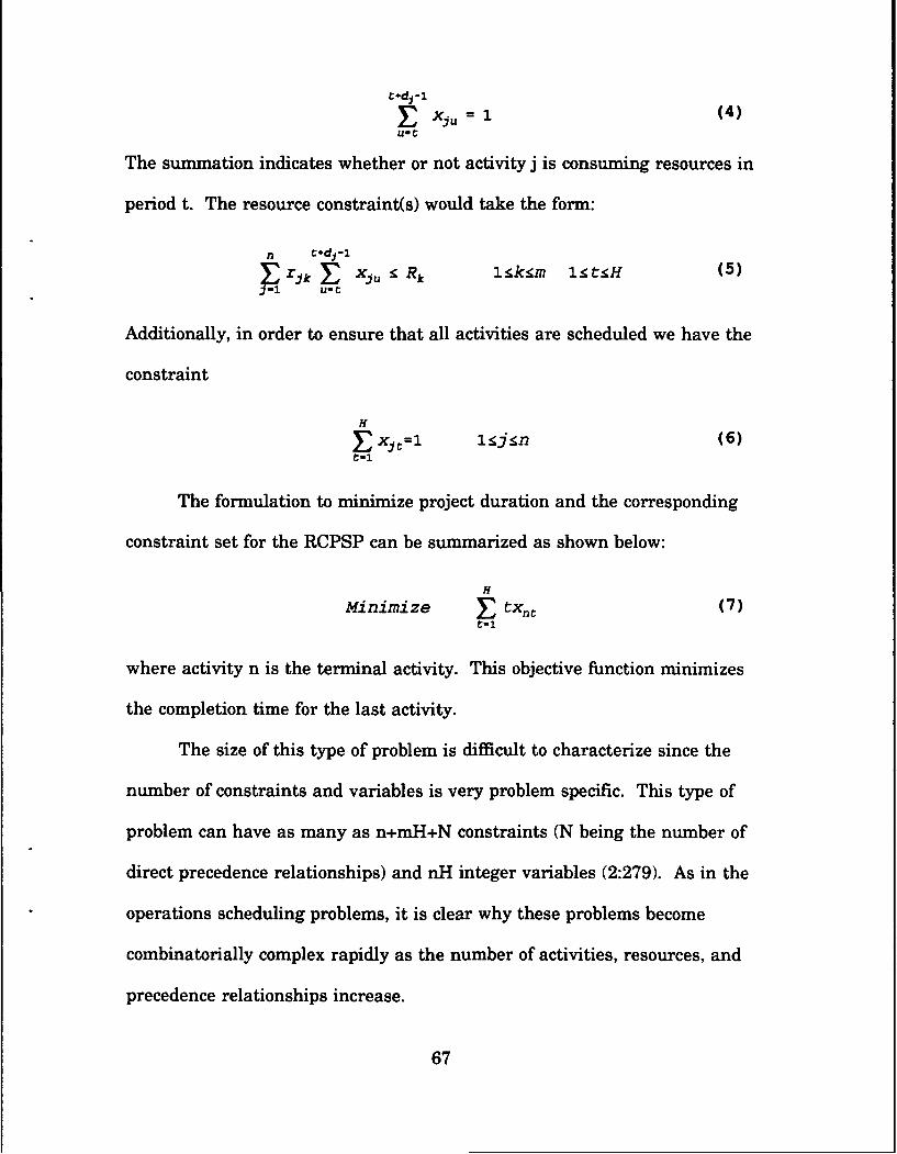
t~dj-l
E j x,,= (4)L1 C
The summation indicates whether or not activity j is consuming resources in
period t. The resource constraint(s) would take the form:
n C+dj-1
E jk xju Rk (5)j-1 u-C
Additionally, in order to ensure that all activities are scheduled we have the
constraint
1Xjljsn (6)
The formulation to minimize project duration and the corresponding
constraint set for the RCPSP can be summarized as shown below:
H
Minimize E tx• (7)C-i
where activity n is the terminal activity. This objective function minimizes
the completion time for the last activity.
The size of this type of problem is difficult to characterize since the
number of constraints and variables is very problem specific. This type of
problem can have as many as n+rmH+N constraints (N being the number of
direct precedence relationships) and nH integer variables (2:279). As in the
operations scheduling problems, it is clear why these problems become
combinatorially complex rapidly as the number of activities, resources, and
precedence relationships increase.
67

Current Techniques and Limitations. The Project Evaluation and
Review Technique (PERT) and the Critical Path Method (CPM) are perhaps
the most well known project scheduling techniques. PERT and CPM
assume that unlimited resources are available for project activities. Hence,
PERT and CPM do not address the resource allocation problem.
The combinatorial nature of the RCPSP makes the search for optimal
solutions unrealistic for most practical problems. Integer programming and
branch and bound techniques have been the focus of most of the research in
this area. However, these techniques are computationally extensive and
remain ineffective for most realistic problems (7:353).
Because of the difficulties associated with analytical techniques,
extensive research has been directed at the development of heuristic
procedures for the RCPSP. While these techniques cannot guarantee
optimal solutions, they can provide "good" solutions for very large problems.
The techniques are normally quick and easy to use. Many can be directly
related to heuristic techniques from job shop scheduling research. A
heuristic procedure is generally a rule, or set of rules, that determines
which activities to schedule, time period by time period, out of a set of
activities that are in contention for limited resources. These resource
contentions are traditionally resolved beginning with an all early start or all
late start schedule. Resource contentions are addressed, one at a time,
working from the first time period (t=1) to the end of the project. A good
68

heuristic procedure is one that minimizes schedule growth, over the critical
path schedule, as the schedule is made resource feasible.
For example, the "total least slack first" heuristic has gained wide
acceptance (7:353). Activities are "ordered" from least available slack to
most available slack, and where resource contention exists, activities with
the least slack are scheduled first (7:353).
Removing the assumptions of a static project initiation, deterministic
activity times, deterministic resource levels, and a deterministic project
network makes the already complex project scheduling problem seemingly
impossible. Simulation has become the main tool used to investigate the
dynamic project initiation, probabilistic activity duration, probabilistic
resource level version of the RCPSP. Simulation, as well as other research
investigating traditional PERT and CPM assumptions, have demonstrated
that current PERT/CPM based scheduling techniques generate critical path
estimates that consistently underestimate project duration (22:68). While
PERT techniques do recognize activity variability, they do not recognize the
fact that path interactions can delay project completion (22:66,68).
Simulation can be used to determine how often probabilistic activities lie on
the project's critical path. These criticality indices give project managers an
indication of how likely it is that any particular activity will delay project
completion. Simulation can also be used to study the effect of alternative
heuristic procedures under probabilistic conditions. Often, results from
predecessor activities will determine which successor activities actually take
69

place. Uncertainty in project network structure can also be simulated
through the use of probabilistic branching (19:145-237).
In short, many of the assumptions required in order to deal with the
RCPSP, can be relaxed through the use of simulation. Many techniques
and software packages use simulation to address the probabilistic project
scheduling problem. The interested reader is referred to Modeling and
Analysis Using Q-GERT Networks by A. Alan B. Pritsker and "A Simulation
Approach to PERT Network Analysis" by Adedeji B. Badiru.
A Comparison of the GJSSP and the RCPSP
In Mathematical Aspects of Scheduling & Applications Bellman,
Esogbue and Nabeshima summarize "mutual relations" between the above
scheduling problems (4:51). According to Bellman, et al. the multiproject
scheduling problem with resource constraints, as a resource allocation
problem, includes the general job shop sequencing problem.
Bellman et al. continue their comparison by asserting that the single
project scheduling problem with a single resource constraint, is related to
the line balancing problem with one exception. This exception is that the
process time for activities expands into many periods and, each work
element is assigned to one work station. The authors state that by dividing
each activity i with activity processing time pi, into pi tasks, each resulting
task will have a unit processing period. The "mutual relations" then
70

correspond completely (4:52) The relationships presented in Table 1 are
extracted from Mathematical Aspects of Scheduling and Applications.
Table 1. Scheduling Problems - Mutual Relations (3:51)
Multiproject Scheduling Problem General Sequencingwith Resource Constraints Problem
Project ........................ JobActivity ....................... Operation (each job on each
machine)Precedence relation .............. OrderingResource ...................... MachineResource availability ............. Number of identical machinesResource Requirements by each
activity ...................... Number of identical machinesthat can process eachoperation
Single Project Scheduling Problem Assembly Line Balancingwith Single Resource Constraint Problem
Unit period .................... Work StationActivity ...................... Work ElementPrecedence relation ............. Precedence RelationResource availability ............ Cycle timeResour-e requirement by eachactivity ..................... Work time of each work
element
Further Classifying the Scheduling Problem. While a comparison of
terminology is useful, it can also be misleading. The assumptions that
characterize the true nature of these scheduling problems must be
examined. While retaining the underlying assumptions of static arrivals
and deterministic processing times, the traditional classification scheme
71
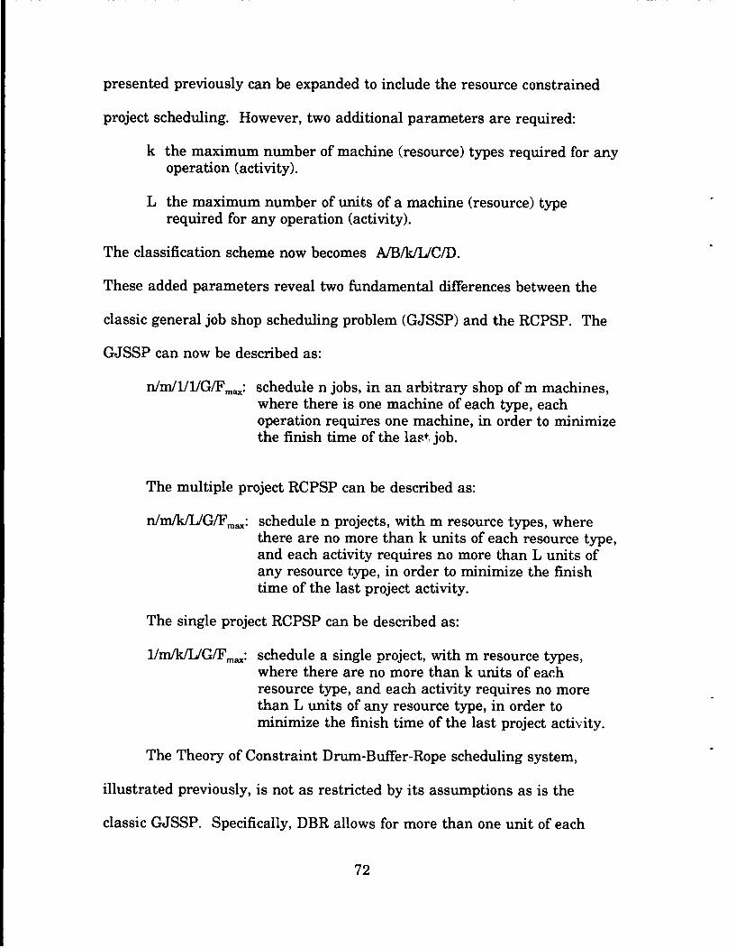
presented previously can be expanded to include the resource constrained
project scheduling. However, two additional parameters are required:
k the maximum number of machine (resource) types required for anyoperation (activity).
L the maximum number of units of a machine (resource) typerequired for any operation (activity).
The classification scheme now becomes A/B/k/L/CID.
These added parameters reveal two fundamental differences between the
classic general job shop scheduling problem (GJSSP) and the RCPSP. The
GJSSP can now be described as:
n/m/1/1/G/F.m.: schedule n jobs, in an arbitrary shop of m machines,where there is one machine of each type, eachoperation requires one machine, in order to minimizethe finish time of the last job.
The multiple project RCPSP can be described as:
n/n~k/fJG/Fm..: schedule n projects, with m resource types, wherethere are no more than k units of each resource type,and each activity requires no more than L units ofany resource type, in order to minimize the finishtime of the last project activity.
The single project RCPSP can be described as:
1/m/k/UG/Fmax: schedule a single project, with m resource types,where there are no more than k units of eachresource type, and each activity requires no morethan L units of any resource type, in order tominimize the finish time of the last project activity.
The Theory of Constraint Drum-Buffer-Rope scheduling system,
illustrated previously, is not as restricted by its assumptions as is the
classic GJSSP. Specifically, DBR allows for more than one unit of each
72

resource type to be available in the shop, and each job can use each
machine as often as required. The fundamental assumption that the Theory
of Constraints and the DBR scheduling system retain from the classic
GJSSP is that each operation can be performed by one unit of one resource.
This important distinction places Theory of Constraints and the DBR
scheduling system in the realm of the GJSSP. Specifically, the Theory Of
Constraints and DBR can be used to address all manufacturing scheduling
problems up to and including the n / m I1I1/ G IF. scheduling problem.
This scheduling problem is clearly more restrictive than the
n I m /k /L I G I F. resource constrained scheduling problem.
In light of the above classification scheme, the RCPSP can be added
to the scheduling problem Venn diagram. The DBR system, while not as
restricted by assumptions to the classic general job shop, remains in the
realm of the GJSSP scheduling problem.
Completing the comparison of the job shop and the project scheduling
problems requires a summary of the characteristics the three scheduling
environments relevant to this research. A summary comparison of these
scheduling problems is presented in Table 2.
73

4)1
7g, 221 Z
r6~- C 4 -- o o> . . ~ ~ 4
os 24 . : .t4 4
Z~o CC aC
U~C C 0 4 CA
C.C
~ 0 0..4L0Cm~ t- I 4-.0
4)3 .. K$.4 0
0b 4)I
0C Ie.-~~~r C .a a a. .
:E -Z a's
0 0 - ca0
E S.
0 0.
as 4-4)
cc tcc0
f~aZ 74

Figure 3. Venn Diagram of Manufacturing and ProjectScheduling Problems
The Theory of Constraints. Project Scheduling and the Critical Chain
Concept
Organizations that have applied the Theory of Constraints' principles
and techniques have realized substantial benefits from doing so. While the
direct benefits are unique to these organizations, the end result is a
significant movement of the organization toward its goal. While a
comprehensive review of the benefits of applying Theory of Constraints to
an organization is beyond the scope of this research effort, the two examples
reviewed in previous sections allude to the benefits that may result from
applying Theory of Constraints to other environments. Manufacturing
based Theory of Constraints principles and tools are being applied to the
project scheduling environment because of the opportunity to achieve
75

similar benefits. The similarities that exist between the RCPSP and the
GJSSP facilitate the application.
The Critical Chain concept is a direct application of the Theory of
Constraints' five step focusing process and the Drum-Buffer-Rope
scheduling system. The Critical Chain concept is a heuristic scheduling
method designed to addresses the RCPSP. The fundamental concept behind
the Critical Chain technique is the identification of critical project
resources. These critical resources are identified as the project constraints.
It is the lack of these resources that delays project completion. Priority is
given to those activities that use these critical resources. Other project
activities are scheduled to "support" those activities using the critical
resources. The principle involved is the same already discussed: make sure
the critical resources are working on the right activities at the right time.
Currently the concept has been applied to the single project scheduling
environment and it is in that light that it will be reviewed.
The development of this heuristic technique appears to have begun
through the Avraham Y. Goldratt Institute during 1990. While the Critical
Chain heuristic is being explored by several researchers, all give conceptual
credit to Dr. Goldratt. Although there is currently no published research on
this technique, unpublished work by Dr. James T. Low and G.D. Bergland
form the fundamental basis for the definition and demonstration of the
method documented in the following chapter. The Critical Chain concept is
76

relatively new, untested, and fairly ill-defined in some areas. The procedure
will undoubtedly evolve further.
The Critical Chain Concept Defined. The Critical Chain algorithm
has as its goal the creation of a "realistic schedule that is immune to a
reasonable level of disruptions" (17:1). The minimization of project cost,
recognizing the net present value concept of cash flow, has also been
mentioned as a possible objective of the Critical Chain scheduling heuristic
(6). The Critical Chain algorithm addresses two fundamental project
scheduling phenomena, resource constraints and the effects of statistical
fluctuation and dependent events, through the application of the five step
focusing process and the Drum-Buffer-Rope scheduling technique. These
techniques have enabled manufacturing firms to effectively reduce the
negative effects these characteristics have on the achievement of the
organization's goal. Their application to the resource constrained project
scheduling problem has been prompted by the similarities in the
characteristics of the two problems.
The purpose of the Critical Chain algorithm is to identify and protect
a project's Critical Chain from various sources of disruption through the
execution of the five step focusing process and the insertion of protective
time buffers. While an exact definition of a project's Critical Chain depends
on the specific application of the Critical Chain concept being considered, it
77

is appropriate to give a general definition at this point'. A project's Critical
Chain can be defined as the set of activities that, due to both technical and
resource precedence constraints, dictate the project's duration (5:1-3). Given
the example project network and the schedule depicted by the Gantt chart
in Figures 4 - 5, the Critical Chain is determined to be S - Al - A2 - D1 - D2
- F (how the Critical Chain has been determined will be addressed in
Chapter III). There are two types of arrows in the network diagram. The
solid arrows represent technical precedence relationships and are the arcs
normally found on PERT network diagrams. The dashed arc is referred to
as a delay arc that has been added to the network to represent a scheduling
decision. The delay arcs are not part of the original network schedule; they
are added to the network as these scheduling decisions are made. In the
schedule in Figure 5, the decision was made to start Al before A2. The
delay arc, in effect, enforces that decision by indicating Al must precede A2.
Figure 5 illustrates how both technical precedence relationships (Dl-D2)
and resource precedence relationships (A1-A2) determine project duration.
The Critical Chain is similar to the project's critical path. The
project's critical path, however, considers only technical relationships and
may contain slack once the schedule has been made resource feasible. The
Critical Chain considers both technical and resource precedence precedences
(represented by delay arcs) and contains no slack.
1 Low's Critical Chain includes protective time buffers. Bergland nor the authors do not include these
protective time buffers.
78

Racmeio Qty AvMWO~iadAB IC1
DAll scdidw rm 1 unit of a .
I (LA aevity Al nquii 1 unof memow A)
DUR
• ~Cd"1C~dn S-AI-A2-D1-2-F
("vity--Nonb Repum=adm)
Figure 4. Sample Network
A CRITICAL CHAIN EXAMPLE
Duration
Critic Al-A2-Di-D2
Figure 5. An Example of A Critical Chain
79

Background. There are, at present, three different applications of
Theory of Constraints to the project scheduling environment that have
adopted the term Critical Chains. The first concept is currently under
development as part of a doctoral dissertation by Mr. Paul Pittman at the
University of Georgia; any specific concepts or algorithms associated with
his development were unavailable for this research. The second application,
advanced by Dr. James T. Low, Associate Professor of Marketing, Wayne
State University, consists of a conceptual framework to address the resource
constrained project scheduling problem (17:1). The third approach is
advanced by Dr. G.D. Bergland of AT&T Bell Laboratories and uses the five
step focusing process of the Theory of Constraints to resolve resource
contentions within a project schedule. The literature that currently exists
on the Critical Chain concept consists of various informal working papers
and a draft dissertation proposal by the above named individuals. As of yet,
there are no publications which document the concepts/techniques
developed. The main focus of this research will be to document the Critical
Chain concept and formally present a Critical Chain algorithm.
The Critical Chain Models.
Pittman's Model. Pittman recognizes the concept of the project
Critical Chain. As part of a unpublished dissertation proposal, Pittman
associates the Critical Chain algorithm with the priority planning function
of project management (18:8). Pittman's research effort is centered on
developing a Theory of Constraints based systems approach to project
80

management that combines the five elements of project planning (18:5).
These elements are project priority, capacity planning, priority control,
capacity control, and master scheduling (18:8). To date, no Critical Chain
algorithm or specific concepts identified with this approach are available.
Once the algorithm is developed, however, Pittman plans to use simulation
to compare the newly developed Theory of Constraints based heuristic with
traditional project management techniques for the RCPSP (18:6).
Low's Model. Low has developed his Critical Chain application
at a conceptual level (no algorithm has been formally documented for
implementing these concepts). According to Low, the Critical Chain:
follow[s] the longest time path backward through the project until a"Critical Chain Buffer" time is encountered, which has been insertedinto the path because of contention for that resource. The [CriticalChain] then 'Jumps" to the path which contains the task that forcedinclusion of the buffer time into the prior path. (17:2)
This definition of the Critical Chain reflects Low's method of
protecting the Critical Chain from disruptions by inserting time buffers
directly into the Critical Chain at every point a non-Critical Chain activity
intersects the Critical Chain. The Critical Chain, therefore, contains both
activities and buffers (Bergland does not include the buffers in the Critical
Chain). The example project network is buffered according to Low's
buffering concepts (discussed later) and is shown in Figures 6 - 7. In Figure
6 below, a Critical Chain buffer is inserted between two previously
contentious Critical Chain activities (Al and A2) where a non-Critical Chain
activity (B1) intersects the Critical Chain. The Critical Chain follows the
81

project path from project completion to activities D2, D1 and A2, at which
point the Critical Chain buffer is encountered. The Critical Chain then
"jumps" to activity Al which, because of the Al - A2 resource contention
Raam Qty Av~iebkVOdA 1BC 1D 1
Low's~f~DUR
Cffm cdlmIin S-Al -A2-D I-D2-F ____ Cc~m
Figure 6. Low's Critical Chain Demonstrated
A CRITICAL CHAIN EXAMPLE
~~C1
JCC -N- bb
DuratonLow. t~
Cica Ch Ail - A2 - D1 -D2 --
Figure 7. Low's Critical Chain and Project Duration
82

and the intersection of activity B1 with the Critical Chain, forced the
insertion of the Critical Chain buffer. The Critical Chain has "jumped" to a
different network path at this point
Low makes a distinction between the primary and secondary Critical
Chains within a project network. The primary Critical Chain is identified
as the
longest time path backward through the project until a 'CriticalChain Buffer' time is encountered. The primary critical chain thenjumps to the path which contains the task that forced inclusion of thebuffer time into the prior path (17:2).
Low defines a secondary Critical Chain as those activities sequenced
as a result of the resolution of resource contentions, that do not define the
longest path through the project schedule. This implies that some activities
sequenced during the Critical Chain procedure will not be included in the
primary Critical Chain. However, a secondary Critical Chain deserves
management attention since disruptions along a secondary Critical Chain
may spread through resource interactions and affect the resource
availability for activities on the primary Critical Chain, delaying project
completion (17:2).
The main focus of Low's application is in the placement and sizing of
time buffers to ensure a "feasible project schedule which is immune to
disruptions" (17:1). The schedule is protected against project disruptions
through the insertion of two types of buffers.
83
A completion buffer is inserted at the end of the resource feasible
schedule to protect the project completion date. The scheduled completion
date of the project, then, is the project duration plus the completion buffer.
The activities on the Critical Chain are protected from the effects of
probabilistic activity durations and other disruptions by a Critical Chain
buffer. Although Low does not discuss buffer sizing mechanisms or
techniques, the Critical Chain buffer must be at least as large as the
completion buffer to ensure adequate protection (17:1).
To ensure the schedule is "immunized," Low inserts buffers as shown
in Figures 5 - 6. Placement of a time buffer between activities Al and A2
ensures the availability of resource A at the scheduled time. There is a
trade off between lengthening the project duration through the use of
buffers and the amount of risk associated with not completing the project on
schedule. According to Low,
any contending task which will wait for a resource to be madeavailable must have a "Critical Chain Buffer" time between itspreceding task's completion time, and the time at which it may beginusing the contended resource. (17:1)
Low also states, "Every path jump requires that a Buffer be inserted into
the new path in front of the task causing the path jump" (17:2).
Implications of the above statements become clearer when viewed in
light of the nature of the Critical Chain. There are a number of paths
available in any given project network that consist of sequential, technically
related activities that can be followed uninterrupted from project beginning
84

to project completion. The Critical Chain will "jump" from path to path and
resource to resource throughout a project network. The fact that the
Critical Chain "jumps" from path to path is a result of the fact that critical
resources are utilized by different activities on different paths. A Critical
Chain "Jump" from one path to another is the result of the utilization of a
critical resource by the activities on both sides of the "jump." As a result, a
Critical Chain buffer is placed within the Critical Chain itself, trading
project duration for protection from project disruptions.
By placing buffers within the Critical Chain, Low implies that the
activities that contribute the most to project completion variance are the
Critical Chain activities. Therefore, the emphasis is placed on protecting
the project completion date from Critical Chain activity duration variances
through the insertion of Critical Chain buffers between Critical Chain
activities.
Bergland's Model. Currently, the most complete application of
the Theory of Constraints concepts to the RCPSP is the Critical Chain
concept proposed by Bergland. Bergland's implementing mechanism is the
five step focusing process and the DBR system. These tools were developed
in the manufacturing environment to minimize the effect of system
constraints and the interactive effects of statistical fluctuations and
dependent events on the organization's goal. Ber-,Iand's application of the
five step focusing process is summarized below.
85

Bergland begins the Critical Chain algorithm with an all late start
project schedule. Bergland recognizes and defines that the constraints in
the RCPSP are the resource contentions that exist within this late start
project schedule. To make a late start schedule resource feasible, each of
these constraints must be exploited or resolved.
While traditional heuristic approaches to the RCPSP use certain
criteria to sequence contentious activities time period by time period,
Bergland's Critical Chain heuristic attempts to minimize the increase in
project duration by enumerating the possible resolutions of the resource
contention, resource by resource. Activities are then buffered to provide
schedules that are immunized against a "reasonable level" of disruptions
and new activity completion dates are scheduled.
Bergland accounts for the fact that there may be more than one
resource contention in any resource constrained project. In order to
determine which contention should be resolved and exploited first,
Bergland's heuristic procedure explicitly enumerates all possible activity
sequences that resolve each contention. The resolved contention that
produces the longest, minimum length Critical Chain is selected as the
system's constraint. The feasible sequence that produces the minimum
length Critical Chain best exploits the identified contention. In effect, the
process of identifying the constraint to be resolved first simultaneously
produces the sequence of activities that best exploits the identified
constraint (5:1).
86

The remaining activities are subordinated to the newly sequenced
activities by scheduling all project activities "around" this sequence.
Critical Chain activities that are technical predecessors of the newly
sequenced activities are scheduled at their late start. Critical Chain
activities that are technical successors of the newly sequenced activities are
scheduled at their late start date. All free paths are scheduled backwards,
or in other words according to the activity late start times (5:1). Buffers are
inserted throughout the network to protect the Critical Chain from activity
duration variances (5:1).
Bergland uses three different types of buffers to protect the Critical
Chain. All activities are initially scheduled to begin on their associated late
start date. This point is critical to the buffering concept, as will be
demonstrated below. The Critical Chain shipping buffer is used to protect
the project's scheduled completion date against all sources of project
duration variance. The shipping buffer is placed at the end of the project
after the last activity is completed (5:1). Bergland's shipping buffer is
identical to Low's completion buffer both in purpose and in location.
Bergland's Critical Chain resource buffer is used to ensure that a
critical resource is available before it is scheduled to be used in the Critical
Chain (4:1). This resource buffer ensures the availability of a resource prior
to its scheduled use in the Critical Chain. In effect, this buffer creates an
early availability date. The resource is made available for use one resource
buffer earlier than required (6). The resource buffer ensures that critical
87

resources are available early in case the preceding activities finish early.
Since this resource is made unavailable for other activities during this
period, and the buffer does not directly appear in the project schedule, care
must be taken when using this implementation to avoid scheduling it on
other activities. Bergland's scheduling heuristic must consider the non-
availability of this resource during the resource buffer period.
A project's Critical Chain may consist of multiple "sets" of sequenced
activities, where each activity in a set requires the same critical resource. A
resource buffer is inserted into the project network at each point where a
change occurs with respect to the critical resource required for the next
Critical Chain activity. This may require the insertion of multiple resource
buffers for the same resource if that resource is used in more than one set
of critical activities.
Figure 8 illustrates the position of shipping and resource buffers in a
sample network. The resource buffers ensure that the associated activities
are able to begin a buffer time earlier than scheduled if all predecessor
activities are completed early.
Assembly Buffers are used to protect the Critical Chain from duration
variances associated with non-Critical Chain activities (5:1). The assembly
buffers are placed at the point at which a "non-Critical Chain path joins a
Critical Chain" (5:1). Bergland's placement of assembly buffers is also
depicted in Figure 8.
88

ROw aze Qty AvI.pmodA 1B 1
CD 1
ScridaiasCuin: S-AI -A2-D I-D2-F L .sus~q•€ti•Nod6 RtetmmkmU) B- a
Figure 8. Bergland's Buffering Concept
It should be noted that there is no equivalent to the elevation step in
Bergland's algorithm. In the manufacturing environment, the elevation
step consists of efforts designed to eliminate a resource as a constraint.
These efforts may include process improvements or changes in the
procedures and/or equipment associated with a particular constraint. In the
RCPSP, the constraint (the resource contention) is exploited by sequencing
the activities in such a way as to make the activities resource feasible.
The objective of the following chapter is to present the Critical Chain
algorithm developed by the authors. The intent is to provide a algorithm
that parallels the Theory of Constraints' techniques and principles
implemented in the manufacturing scheduling problem, to the degree that
the application of these concepts is both possible and logical. The algorithm
89

has not been evaluated or compared to other resource constrained project
scheduling techniques.
90

III. The Critical Chain Algorithm
Overview
This chapter details the Critical Chain algorithm developed as a
result of the authors' review and understanding of the Theory of
Constraints, the RCPSP and the Critical Chain literature. The five step
focusing process developed in the manufacturing environment serves as the
basis for this implementation of the Theory of Constraints concepts to the
RCPSP.
The first section of the chapter will provide a brief overview of the
Critical Chain algorithm. This discussion describes the objectives and the
expected output of each step. The final product of the algorithm is a
resource feasible schedule that is immune to project disruptions. The
second section of the chapter presents the Critical Chain algorithm.
Finally, the last section demonstrates the algorithm using an eight activity
project.
The Critical Chain Algorithm
The Critical Chain concept recognizes the importance of protecting
the longest time path of a resource feasible project schedule from the
disruptions that may delay the project beyond its scheduled completion
date. The Critical Chain procedure, like its parent DBR procedure,
schedules by focusing on the resource (and in particular the constraining
91

resource) first, whereas all previous procedures focus on the
activities/operations first. Only then are resource problems dealt with,
almost as an afterthought. The schedule is made realistic (resource
feasible) by iteratively sequencing the activities that are in contention for
limited resources. The sequence of these activities is chosen based on the
net effect the sequence has on project duration. Buffers are then
strategically placed within the network to protect against disruptions and to
ensure the timely availability of resources involved in the Critical Chain.
While Bergland and Low present similar, fundamental aspects of the
Critical Chain concept, they have not reached a consensus regarding a
specific algorithm or procedure that implement the concept. The algorithm
that follows was derived from Bergland's approach, Low's concept and the
researchers' understanding of the Theory of Constraints and the RCPSP.
An Overview of the Critical Chain Algorithm. The Critical Chain
concept applies the five step focusing process to the RCPSP. While each of
the five steps cannot be directly applied to the RCPSP, the intent and
underlying principles of the focusing process is maintained to the greatest
extent possible. An overview of each of the five steps is provided below.
Chapter IV will provide the rationale supporting each step and will also
illustrate the Theory of Constraints basis for each step.
Step 0. Initialize Project Data Set. The Critical Chain
algorithm requires certain project information. This information includes
mean activity durations, activity precedence relationships, activity resource
92

requirements, and resource types and availabilities. A network
representation of the project, a late start schedule, and the associated
resource utilization profiles are developed based on this information. If the
late start schedule is resource feasible, no further steps are taken. The
following project conventions and assumptions apply to the algorithm2 :
- Activity durations are stochastic- Precedence relationships are known- Resource requirements per activity are known with certainty- Resource limits are known with certainty- Each activity requires the use of only one of the resource types- Early Start times are denoted by ES- Late Start times are denoted by LS- Early Finish times are denoted by EF- Late Finish times are denoted by LF
The following definitions apply to the algorithm. Let:
- J represent the set of all activities in the project,- j denotes the job index j e (J),- Let K represent the number of resource types,- k denotes the resource index, k = 1,..,K- w denotes a window of contention consisting of consecutive time
periods in the scheduling horizon in which a contention for aresource exists between two or more activities.
Step 1. Identify the Constraint. A constraint is defined as a
resource contention. These contentions must be prioritized to determine
which one to resolve first. Assign the highest priority to the activities
associated with that contention which has the greatest excess demand.
Excess demand is calculated for each period in the scheduling horizon of a
2The following timing convention has been adopted. Start and finish times are defined as the end of theperiod. For example, a 3 period activity may have a start time of 1 and a finish time of 4. This means that theactivity starts at the completion of period 1, is in process in periods 2,3 and 4, and finishes at the end of period4.
93

given schedule for each resource type. The excess demand in a period is 0 if
resource availability meets or exceeds the cumulative resource demand of
all activities in process in that period. Otherwise, excess demand for that
period is the difference between the cumulative resource demand and
resource availability in that period. In Figure 9, for example, there is 0
excess demand for resource A in all periods except periods 17 - 20 since
resource availability meets or exceeds resource demanded in all but these
periods. During periods 17 - 20 the demand exceeds availability in each
period by 1 unit of resource A. Therefore, excess demand is equal to 1 in
periods 17-20. The cumulative excess demand for resource A is then 3
units.
The identification of the highest priority contention is accomplished
in a three step process. First, identify the resource (k*) that has the
greatest cumulative excess demand over the entire scheduling horizon.
Second, identify the windows of contention (w) associated with the k"
resource. A window of contention is a period or a combination of
consecutive periods in which the demand for k* exceeds the amount of k*
available. Third, the activities associated with the window (w) having the
greatest excess demand is identified as the set of j activities. The j*
activities in contention for the k* resource during the window of greatest
contention (w) will be sequenced first.
94

ONE UNIT OF RESOURCE A AVAUABLE PER PEROD
S 10 15 20
ME PERIOD
Figure 9. Excess Demand Demonstrated
Step 2. Exploit the System Constraint. Once the set of jf
activities has been identified as the constraint, it must be exploited. In the
RCPSP, this translates to resolving the priority contention identified in Step
1 in such a way as to minimize project duration. In the Critical Chain
algorithm, all technically possible sequences of j" activities that resolve the
contention are explicitly enumerated. The sequence of activities resulting in
the shortest project duration, defined as a lower bound on project duration,
is selected as the sequence of j" activities that best exploits the k* resource.
The network is updated with delay arcs representing the resource
precedence relationships established by this sequence.
Step 3. Subordinate. The remaining project activities are
made subordinate to the sequence of j activities. The new project schedule
resulting from the sequenced j" activities is determined. The f activities are
95

scheduled using their respective early start dates. Predecessors to the
sequenced j* activities are scheduled using their respective late start.
Successors to the sequenced j* activities are scheduled using their respective
early start dates. Free activities are scheduled using their late start dates.
In this way, the activity start times are "packed" around the Critical Chain
in the same manner that the processing order of the constraint is "packed"
in the manufacturing environment to eliminate any periods of time in which
the constraint is not being utilized. The Critical Chain is defined as the
sequence of activities that, due to resource and precedence relationships,
constitute the longest duration through the network. New resource
utilization profiles are developed based on the newly developed project
schedule. If the project remains resource infeasible, another iteration is
accomplished starting with Step 1. If no resource contentions exist, the
Critical Chain must be protected by the insertion of buffers as described in
Step 4.
Step 4. Immunize the Critical Chain. The Critical Chain is
protected from disruptions by inserting three types of buffers. The
implementation of the buffering concept is consistent with Bergland's
approach. A shipping buffer (SB) is inserted at the end of the project to
protect the completion date. An assembly buffer (AB) is inserted at any
point a non-Critical Chain activity intersects the Critical Chain. Resource
buffers (RB) are inserted to ensure the instant availability of the resource
when it is required for the Critical Chain (assuming the buffer size is equal
96

to or larger than the activity variance). Update the project network and
resource utilization profiles to reflect the insertion of these buffers.
Step 5. Elevate. In a manufacturing environment, a CCR
constraint is elevated by any effort focused on increasing the capacity of the
constraint. If the project manager is not satisfied with the scheduled
project duration, some adjustment must be made to the project. Elevation
may include the purchase of additional resources, an adjustment to the
scope of the project, etc. Table 3 summarizes the objectives and required
output of each algorithm step.
97

4) W~ w-~
4.3 *-U)UC
r- ,0.m
a) 6a) . Q .
a) 0 0. 0. V.*cI CD $
-4) 4)-a a
0o , :% 0 Q~
P. 4 4 a) 4)cF Pi nc
o xu U03 c
- rA) 2 Cu5 CISC
U Cu ) a) 098
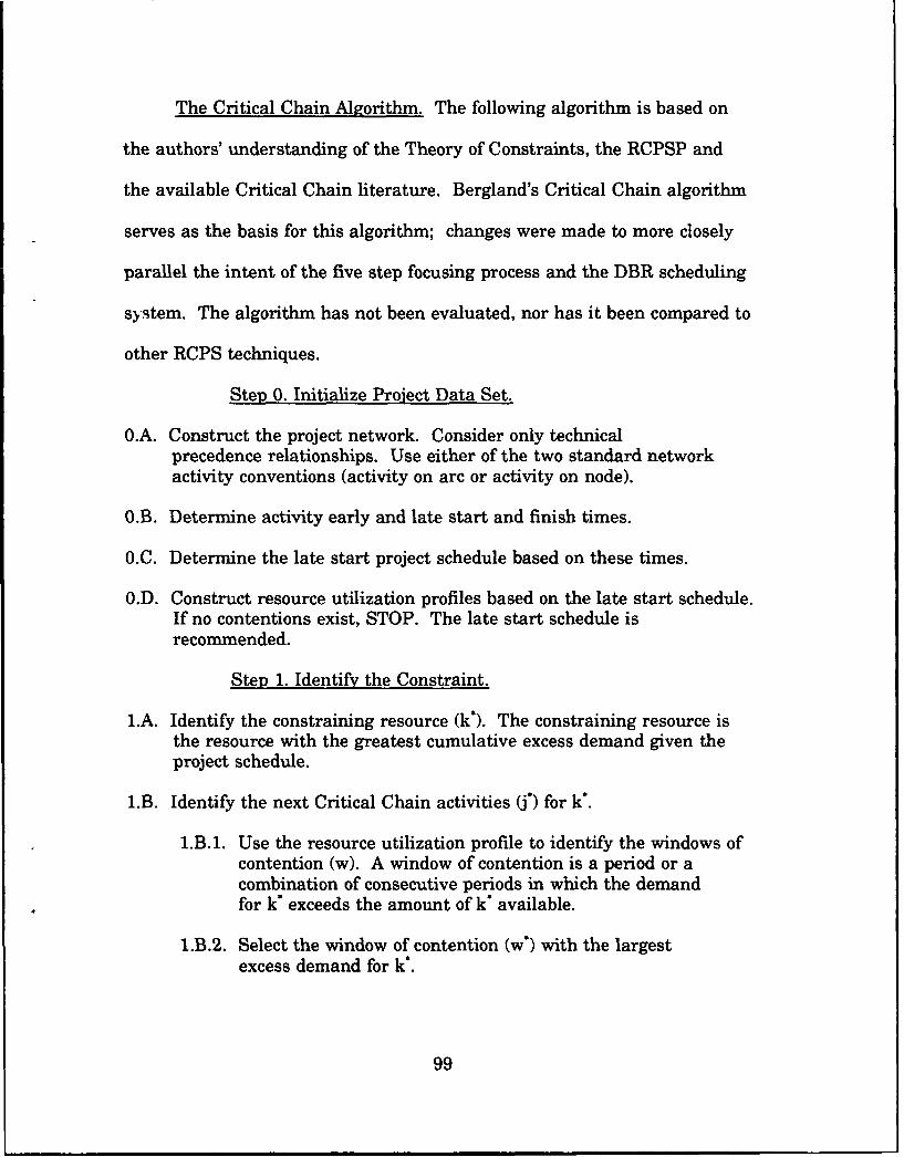
The Critical Chain Algorithm. The following algorithm is based on
the authors' understanding of the Theory of Constraints, the RCPSP and
the available Critical Chain literature. Bergland's Critical Chain algorithm
serves as the basis for this algorithm; changes were made to more closely
parallel the intent of the five step focusing process and the DBR scheduling
system. The algorithm has not been evaluated, nor has it been compared to
other RCPS techniques.
Step 0. Initialize Project Data Set.
0.A. Construct the project network. Consider only technicalprecedence relationships. Use either of the two standard networkactivity conventions (activity on arc or activity on node).
O.B. Determine activity early and late start and finish times.
0.C. Determine the late start project schedule based on these times.
0.D. Construct resource utilization profiles based on the late start schedule.If no contentions exist, STOP. The late start schedule isrecommended.
Step 1. Identify the Constraint.
L.A. Identify the constraining resource (k*). The constraining resource isthe resource with the greatest cumulative excess demand given theproject schedule.
L.B. Identify the next Critical Chain activities (j*) for k*.
1.B. 1. Use the resource utilization profile to identify the windows ofcontention (w). A window of contention is a period or acombination of consecutive periods in which the demandfor k" exceeds the amount of k* available.
1.B.2. Select the window of contention (w°) with the largestexcess demand for k*.
99

1.B.3. Identify as j* the set of activities that are in contention for k"
during the selected window w*.
Step 2. Exploit the System Constraint.
2.A. Enumerate the minimal sequences of j* activities that resolve theresource contention3.
2.B. Evaluate each sequence to determine the project duration. Calculate alower bound on project duration through the following process:
2.B.1. Add delay arcs to the network diagram to implement thesequence.
2.B.2. Calculate the longest path through the modified network.This path length is a lower bound on project duration.
2.C. Select the sequence that yields the minimum lower bound on projectduration to best exploit the constraint.
2.D. Add delay arcs to the network to implement the selected sequence.
Step 3. Subordinate.
3.A. Calculate the early and late start and finish times for all activities.
3.B. Determine the new project schedule.
3.B.1. Assign j* activities to their early start times.
3.B.2. Assign all successors to j* to their ES times.
3.B.3. Assign all predecessors to j" to their LS times.
3.B.4. Assign all free activities to their LS times.
3.B.5. Assign activities that are both a predecessor and a successor tothe set of j" activities to their ES times.
3.C. Determine the longest path through the network. The activities onthis path represents the project's Critical Chain.
3 A minimal sequence is one in which no activity in the sequence can be left-shifted to reduce elapsedduration.
100

3.D. Revise the resource utilization profile to reflect the new schedule.
3.E. Is the schedule resource feasible?
3.E.1. If Yes, go to step 4.
3.E.2. If No, go to step 2.
Step 4. Immunize the Critical Chain.
4.A. Insert a shipping buffer at the end of the project.
4.B. Insert an assembly buffer at every point in the network where a non-Critical Chain activity intersects the Critical Chain. The buffer isinserted between the non-Critical Chain activity and the CriticalChain activity that it feeds. Resource precedent activities, depicted bydelay arcs, must be buffered as well.
4.C. Insert a resource buffer in front of a Critical Chain activity if:
4.C.1. The Critical Chain activity using that resource is the first of asequential series of activities using that resource in theCritical Chain, or
4.C.2. The Critical Chain activity using that resource is not precededor succeeded by an activity using the same resource.
4.D. Update the project network, schedule, and the resource utilizationprofiles to reflect the final schedule. Schedule all non-Critical Chainactivities using their late start dates.
Step 5. Elevate.
5.A. If the schedule is unacceptable,
-- Purchase more resources to reduce project duration,
-- Adjust the project's scope and/or content,
-- etc.
101
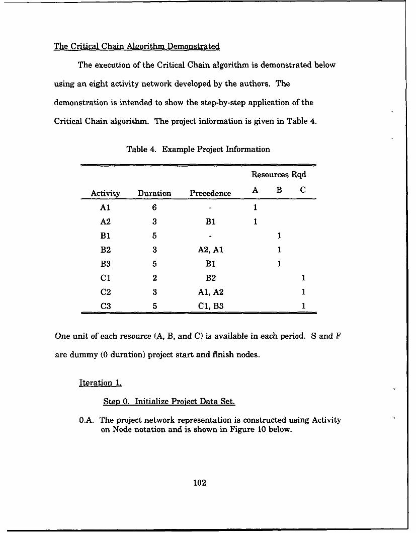
The Critical Chain Algorithm Demonstrated
The execution of the Critical Chain algorithm is demonstrated below
using an eight activity network developed by the authors. The
demonstration is intended to show the step-by-step application of the
Critical Chain algorithm. The project information is given in Table 4.
Table 4. Example Project Information
Resources Rqd
Activity Duration Precedence A B C
Al 6 - 1
A2 3 B1 1
B1 5 1
B2 3 A2, A1 1
B3 5 B1 1
Cl 2 B2 1
C2 3 Al, A2 1
C3 5 C1, B3 1
One unit of each resource (A, B, and C) is available in each period. S and F
are dummy (0 duration) project start and finish nodes.
Iteration 1.
Step 0. Initialize Project Data Set.
0.A. The project network representation is constructed using Activityon Node notation and is shown in Figure 10 below.
102

EXAMPLE NETWORK6 3
Figure 10. Example Network Problem
O.B. The activity early and late start and finish times are determinedwith a standard forward and backward scheduling pass. Notethat the conventional Critical Path for this project is S-B 1-A2-B2-C1-C3-F with a project length of 18 periods. The CriticalChain is the Critical Path at this point.
0.C. The late start schedule consists of the highlighted activity timesshown in Table 5.
0.D. The resource utilization profiles are developed based on the latestart and finish times. The profiles are shown in Figure 11.
Step 1. Identify the Constraint.
l.A. Identify the constraining resource (k'). The constrainingresource is the resource with the greatest cumulativeexcess demand given the schedule. The excessdemand, expressed in resource days, is given below for eachresource.
103

Table 5. Initial Schedule Data
Activity Dur ES EF LS LF
Al 6 0 6 2 8
A2 3 5 8 5 8
B1 5 0 5 0 5
B2 3 8 11 8 11
B3 5 5 10 8 13
C1 2 11 13 11 13
C2 3 8 11 15 18
C3 5 13 18 13 18
A 2 ALZ
Al
1 , I2 3
C2"
I I ' ' ' : ' ' ' I :5 10 15 20
TIM
Figure 11. Resource Utilization Profiles (Iteration 1)
104

Table 6. Cumulative Excess Demand (Iteration 1)
Resource Cum Excess Demand(Resource Days)
A 3
B 3
C 3
Since all three resources are experiencing the same excessdemand, resource A is arbitrarily chosen as the criticalresource, k* = A.
1.B. Identify the next Critical Chain activities (0) for k*:
1.B.1. Use the resource utilization profile (Figure 11) toidentify the windows of contention (w). There is onlyone window of contention for k*. The window occursbetween periods 5-8 and is denoted by w,.
1.B.2. Select the window of contention (w) with the greatestexcess demand. The window of greatest contention, w*,is w, between periods 5-8.
L.B.3. Identify as j the set of activities that are in contentionfor k* during the selected window w*. The j" activitiesare Al and A2.
j {AlM2}
Step 2. Exploit the System Constraint.
2.A. Enumerate the minimal sequences of j activities that resolvethe resource contention. The contention can be resolved bysequencing the j" activities as follows:
Al - A2 or A2 - Al
2.B. Evaluate each sequence to determine the project duration.Calculate a lower bound on project duration through thefollowing process:
105

2.B.1. Add delay arcs to the network diagrams to implementeach of the possible sequences. The delay arcs areshown in Figures 12 - 13.
2.B.2. Calculate the longest path through the modifiednetwork for each enumeration. This path length is alower bound on project duration. Since only projectduration is required at this point, only a forwardscheduling pass will be completed. The early start(ES) and early finish (EF) dates for each enumerationare presented in Table 7. The project duration of eachsequence is provided in Table 8.
EXAMPLE NETWORK(A;d,** on Node)
Figure 12. Sequence Al - A2 (Iteration 1)
106

EXAMPLE NETWORK(AcSvity on No*.
Al 0 C2 A 8 1
3
5 12
Ciur 13.Sqe 2 14- A 1 7(trto 19
C2 9 2 02 1 1
C3 14 19 C3 19 24
107

Table 8. Project Durations (Iteration 1)
Sequence Project DurationA1 - A2 19A2 - A1 24
2.C. Select the sequence that yields the minimum lower bound on projectduration. The sequence yielding the minimum lower bound on projectduration is sequence Al - A2. This is selected as the sequence ofactivities that best exploits the constraint.
2.D. Add delay arcs to the network to implement the selected sequence.The delay arcs that implement this sequence are added to the networkas shown in Figure 12. The additional resource precedencerelationships are shown in Table 9.
Table 9. Project Precedence Requirements (Iteration 1)
Technical ResourceActivity Predecessors Predecessors
Al
A2 B1 Al
B1
B2 Al, A2
B3 B1
C1 B2
C2 Al, A2
C3 C1, B3
Step 3. Subordinate.
3.A. Calculate the early start and finish times for all activities asshown in Table 10.
108

3.B. Determine the new project schedule, as highlighted in Table 10,to include:
3.B. 1. The early start and finish times for all newly sequenced j*activities.
3.B.2. The early start and finish times for all activities that aretechnical or resource successors of the newly sequenced j*activities.
3.B.3. The late start and finish times for all activities that aretechnical or resource predecessors of the newly sequenced j*activities.
3.B.4. The late start and finish times for all free activities.
3.B.5. The ES time if an activity is both a predecessor and asuccessor to the set of j" activities.
Table 10. Project Schedule Information (Iteration 1)
Activity Type ES EF LS LF
Al 0 6 0 6
A2 j 6 9 6 9
B1 Predecessor 0 5 1 6
B2 Successor 9 12 9 12
B3 Free 5 10 9 14
C1 Successor 12 14 12 14
C2 Successor 9 12 16 19
C3 Successor 14 19 14 19
3.C. Determine the longest path through the network. The activities onthis path represent the Critical Chain and includes activities S - Al -A2 - B2- C1 - C3 - F. The network is shown in Figure 14.
3.D. Revise the resource utilization profile to reflect the new schedule. Theupdated resource utilization profiles are shown in Figure 15.
109

EXAMPLE NETWORK(Aodft ~on Node)
2C
2-
C
5 10 15 20
Figure 15. Resource Utilization Profile (Iteration 1)
3.E. Is the revised schedule resource feasible? Figure 15 reveals onecontention that makes the schedule resource infeasible. Therefore asecond iteration is required.
110

Iteration 2.
Step 1. Identify the Constraint.
L.A. Identify the constraining resource (k*) from Figure 15. Theconstraining resource is the resource with the greatest cumulativeexcess demand given the schedule. The excess demand, expressed inresource days, is given below for each resource.
Table 11. Cumulative Excess Demand (Iteration 2)
Cum Excess DemandResource (Resource Days)
B 3
Since resource B is the only resource with cumulative excess
demand, k* is chosen as resource B.
1.B. Identify the next Critical Chain activities (j*) for k*.
1.B.1. Use the resource utilization profile (Figurel5) to identify thewindows of contention. There is only one window ofcontention for k*. The window occurs between periods 8-11and is denoted by wl.
1.B.2. Select the window of contention (w) with the largestexcess demand for k*. The window of greatestcontention, w*, is w, between periods 8-11.
1.B.3. Identify as j* the set of j* activities that are in contention for k*during the selected window w*. The j* activities are activitiesB2 and B3.
j- {B2, B3}
Step 2. Exploit the System Constraint.
2.A. Enumerate the minimal sequences of j" activities that resolve theresource contention. The contention can be resolved bysequencing the j* activities as follows:
111

B2 - B3 or B3 - B2
2.B. Evaluate each sequence to determine the project duration. Calculatea lower bound on project duration for each of the enumeratedsequences.
2.B. 1. Add delay arcs to the network diagram to implement each ofthe possible sequences. The delay arcs are shown in Figures16- 17.
2.B.2. Calculate the longest path through the network for eachenumeration. Since only project duration is required at thispoint, only a forward scheduling pass will be completed. Theearly start (ES) and early finish (EF) dates for eachenumeration are listed below. The project duration of eachsequence is given below.
EXAMPLE NETWORK(Activity on Nods)
6 3
3
Figure 16. Sequence B2 - B3 (Iteration 2)
112
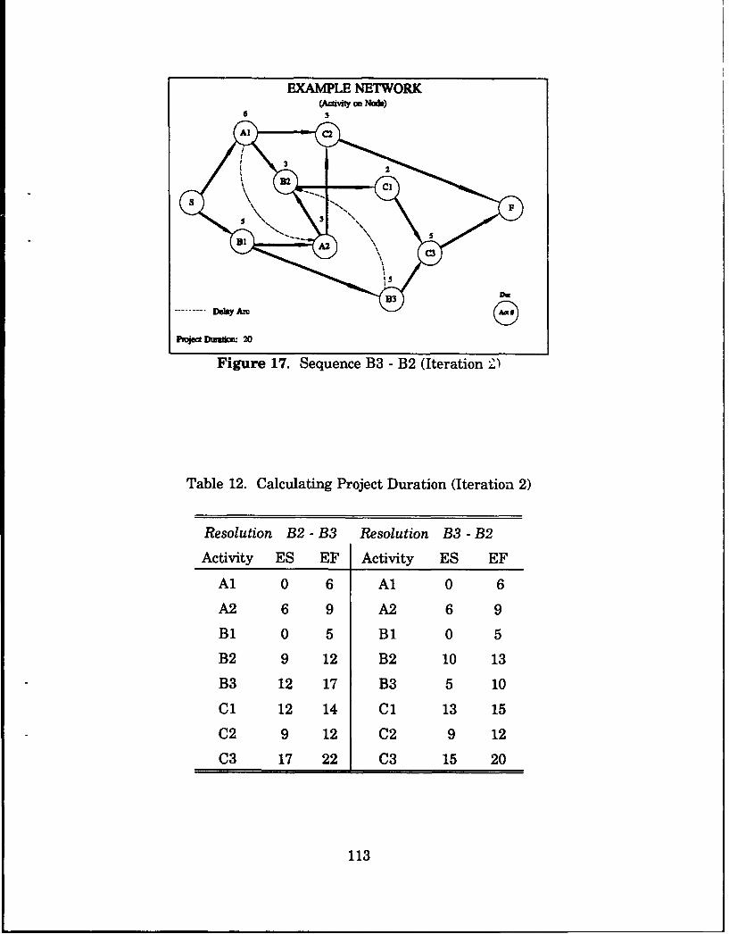
EXAM.LE NETWORK(Acilvity on Node)
6 3
Figure 17. Sequence B3 - B2 (Iteration 2)
Table 12. Calculating Project Duration (Iteration 2)
Resolution B2 - B3 Resolution B3 - B2
Activity ES EF Activity ES EFAl 0 6 Al 0 6
A2 6 9 A2 6 9B1 0 5 B3 0 5
B2 9 12 B2 10 13
B3 12 17 B3 5 10C1 12 14 Cl 13 15
C2 9 12 C2 9 12C3 17 22 C3 15 20
113

Table 13. Project Durations (Iteration 2)
Sequence Project DurationB2 - B3 22B3 - B2 20
2.C. Select the sequence that yields the minimum lower bound onproject duration. The sequence yielding the minimum lowerbound is sequence B3 - B2 (20).
2.D. Add delay arcs to the network to implement the selectedsequence. The delay arcs that implement this sequence areadded to the network as shown in Figure 17. The additional resourceprecedence relationships are shown in Table 14.
Table 14. Project Precedence Requirements (Iteration 2)
Technical ResourceActivity Predecessor Predecessors
Al -
A2 B1 Al
B1 -
B2 Al, A2 B3
B3 B1 -
C1 B2 -
C2 A1, A2 -
C3 C1, B3 -
Step 3. Subordinate.
3.A. Calculate the early start and finish times finish times for each activityas shown in Table 15.
3.B. Determine the new project schedule, as highlighted in Table 15,to include:
114
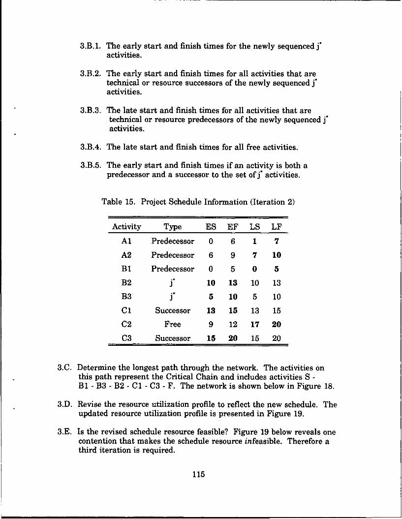
3.B. 1. The early start and finish times for the newly sequenced j"activities.
3.B.2. The early start and finish times for all activities that aretechnical or resource successors of the newly sequenced j"activities.
3.B.3. The late start and finish times for all activities that aretechnical or resource predecessors of the newly sequenced j"activities.
3.B.4. The late start and finish times for all free activities.
3.B.5. The early start and finish times if an activity is both apredecessor and a successor to the set of j" activities.
Table 15. Project Schedule Information (Iteration 2)
Activity Type ES EF LS LF
Al Predecessor 0 6 1 7
A2 Predecessor 6 9 7 10
B1 Predecessor 0 5 0 5
B2 j" 10 13 10 13
B3 f" 5 10 5 10
C1 Successor 13 15 13 15
C2 Free 9 12 17 20
C3 Successor 15 20 15 20
3.C. Determine the longest path through the network. The activities onthis path represent the Critical Chain and includes activities S -B1 - B3 - B2 - C1 - C3 - F. The network is shown below in Figure 18.
3.D. Revise the resource utilization profile to reflect the new schedule. Theupdated resource utilization profile is presented in Figure 19.
3.E. Is the revised schedule resource feasible? Figure 19 below reveals onecontention that makes the schedule resource infeasible. Therefore athird iteration is required.
115

EXAMPLE NETWORK(Acdftt an Nods)
2A
Alca Chi 2tvd
A A
2
C C
5 10 15 20Tmm
Figure 19. Resource Utilization Profiles (Iteration 2)
116

Iteration 3.
Step 1. Identify the Constraint.
L.A. Identify the constraining resource k* using Figure 19. Theconstraining resource is the resource with the greatest cumulativeexcess demand. The only resource experiencing excess demand, isresource C. The excess demand, expressed in resource days, is givenbelow.
Table 16. Cumulative Excess Demand (Iteration 3)
Resource Cum Excess Demand(Resource Days)
C 3
1.B. Identify the next Critical Chain activities (j*) for k*.
1.B.1. Use the resource utilization profile (Figure 19) to identify thewindows of contention. There is only one window ofcontention for k*. The window occurs between periods 17 - 20.
1.B.2. Select the window of contention (w') with the largestcumulative excess demand for k*. Since there is only onewindow of contention, w* occurs between periods 17 - 20.
1.B.3. Identify as j* the set of j activities that are in contention for k"during the selected window w*. The j" activities are activitiesC2 and C3.
j" {C2, C3}
Step 2. Exploit the System's Constraint.
2.A. Enumerate the minimal sequences of j" activities that resolve theresource contention. The contention can be resolved bysequencing the j" activities as follows:
C2 - C3 or C3 - C2
117

2.B. Evaluate each sequence to determine the project duration. Calculatethe lower bound on project duration for each of the enumeratedsequences.
2.B.1. Add delay arcs to the network diagrams to implement eachof the possible sequences. The delay arcs are shown inFigures 20 - 21.
2.B.2. Calculate the longest path through the modified network foreach enumeration. This path length is a lower bound onproject duration. The early start (ES) and early finish (EF)times for each enumeration are listed below in Table 17. Theproject duration of each sequence is given in Table 18.
EXAMPLE NETWORK(Activily on Nods)
3
PqntD a tlL 20,
I I
Figure 20. Sequence C2 - C3 (Iteration 3)
118

EXAMPLE NETWORK4Adctif on No&.)
6 3
Figure 21. Sequence C3 - C2 (Iteration 3)
Table 17. Calculating Project Duration (Iteration 3)
Resolution C72 - C73 Resolution C3 - C72
Activity ES EF Activity ES EF
A1 0 6 Al 0 6
A2 6 9 A2 6 9
B1 0 5 Bi 0 5
B2 10 13 B2 10 13
B3 5 10 B3 5 10
C1 13 15 Cl 13 15
C2 9 12 C2 20 23C3 15 20 C3 15 20
119

Table 18. Project Durations (Iteration 3)
Sequence Project DurationC2 - C3 20C3 - C2 23
2.C. Select the sequence that yields the minimum lower bound onproject duration. The sequence yielding the minimum lower bound onproject duration is sequence C2 - C3. This is selected as the sequenceof activities that best exploits the constraint.
2.D. Add delay arcs to the network to implement the selectedsequence. The delay arcs that implement this sequence areadded to the network as shown in Figure 20. Theadditional resource predecessors are shown in Table 19.
Table 19. Project Precedence Requirements (Iteration 3)
Activity Technical New ResourcePredecessors Predecessors
Al
A2 B1 Al
B1
B2 A1, A2 B3
B3 B1
C1 B2
C2 A1, A2
C3 C1, B3 C2
Step 3. Subordinate.
3.A. Calculate the early and late start and finish times for each activity.The early and late start and finish times are calculated for eachactivity and are shown in Table 20.
120

3.B. Determine the new project schedule as highlighted in Table 20to include:
3.B.1. The early start and finish times for all of the newly sequencedj" activities.
3.B.2. The early start and finish dates for all activities that aretechnical or resource successors of the newly sequenced j"activities.
3.B.3. The late start and finish times for all activities that aretechnical or resource predecessors of the newly sequenced j"activities.
3.B.4. The late start and finish times for all free activities.
3.B.5. The early start time if an activity is both a predecessor and asuccessor to the set of i" activities.
Table 20. Project Schedule Information (Iteration 3)
Activity Type ES EF LS LF
Al Predecessor 0 6 1 7
A2 Predecessor 6 9 7 10
B1 Predecessor 0 5 0 5
B2 Predecessor 10 13 10 13
B3 Predecessor 5 10 5 10
C1 Predecessor 13 15 13 15
C2 j' 9 12 17 20
C3 15 20 15 20
3.C. Determine the longest path through the network. The activities onthis path represents the Critical Chain and still follows activities S -B1 - B3 - B2 - C1 - C3 - F. This remains the project's Critical Chain.The network is shown in Figure 22.
121

3.D. Revise the resource utilization profiles to reflect the newschedule. The updated resource utilization profiles are shown inFigure 23.
3.E. Determine if the revised schedule is resource feasible. Figure 23reveals that no further contentions exist within the project.Therefore, no more iterations are required.
EXAMPLE NErWORK(Aiviy on Nod&)
3
Figure 22. Project Network (Iteration 3)
122

2--
A
Al A2
2B
2--C
;~ EE ; ffM.O: .M.
1 . . . I - ' 1 1 t -
5 to is 20
Figure 23. Resource Utilization Profile (Iteration 3)
Step 4. Immunize the Critical Chain.
4.A. Insert a shipping buffer at the end of the project.
4.B. Insert an assembly buffer at every point in the network where a non-Critical Chain activity intersects the Critical Chain. The buffer isinserted between the non-Critical Chain activity and the CriticalChain activity that it feeds. Resource precedent activities, depicted bydelay arcs, must be buffered as well. In Figure 24, redundant arcs4
have been eliminated from the project network to facilitateunderstanding of assembly buffer placement.
4.C. Insert a resource buffer in front of a Critical Chain activity if:
4.C.1. The Critical Chain activity using that resource is the first of asequential series of activities using that resource in theCritical Chain, or
4.C.2. The Critical Chain activity using that resource is not precededor succeeded by an activity using the same resource.
4 A redundant arc is any network arc (representing either a resource or technical relationship) that canbe eliminated from the network without misrepresenting or violating technical or resource constraints.
123

4.D. Update the project network, project schedule and the resourceutilization profiles to reflect the final schedule. Schedule all non-Critical Chain activities using their late start dates.
The final project network representation and project resource
utilization profiles are shown in Figures 24 - 26. The final network
schedule is shown in Table 21.
EXAMPLE NETWORKL.4CUfty an Node)
124

EXAMPLE NETWORKAcdvity on Node)
ot• Dum2 21 3-:S
Figure 25. Final Network, Redundant Arcs Removed
AB - Amemb1Y P
2-A Catmal Chain AcbUv'A
Al I A
I•2° Lai
2.. ' .... . ........... ... ; ; ; I
C:1
II
5 10 15 20
Figure 26. Final Project Resource Utilization Profiles
125

Table 21. Final Project Schedule Information
Activity ES EF LS LF
Al 0 6 1 7
A2 6 9 7 10
B1 0 5 0 5
B2 10 13 10 13
B3 5 10 5 10
C1 13 15 13 15
C2 9 12 17 20
C3 15 20 15 20
126

IV. Findings and Analysis
Overview
Dr. Goldratt might classify the Critical Chain concept as a paradigm
shift in resource constrained project scheduling. He describes a paradigm
shift as a dramatic change in how a subject is perceived or conceptualized.
A paradigm shift may result in a drastic change and invariably generates
many new questions (13:63). The paradigm shift provides the opportunity
to view the subject from a different perspective; questions arise because of
the new and unfamiliar viewpoint.
The Critical Chain concept departs most dramatically from
traditional RCPSP heuristic techniques by prioritizing the resolution of
resource contentions rather than resolving contentions sequentially, by time
period. Resource contentions are prioritized recognizing that the shortage of
critical resources prevents an earlier project completion date. The second
dramatic departure is the concept of providing buffers to protect the
scheduled project completion date. The Critical Chain concept certainly
creates, and require answers to, many new questions. This is due, in part,
to the infancy of the concept, but a . ro the unfamiliar perspective.
The first section of this chapter will address specific steps in the
Critical Chain algorithm presented in Chapter III. Criterion developed for
each of the five focusing steps are examined, as are alternative criterion for
particular steps. Analogies to the five step focusing process and the DBR
127
scheduling system are scrutinized. Where appropriate, significant
differences from the Low and Bergland concepts are delineated.
The second half of this chapter will address fundamental issues
raised during the study of the various Critical Chain concepts and in the
development and execution of the algorithm outlined in Chapter III. Both
conceptual and implementation issues are examined. The leading segment
of this section addresses what the authors feel is the fundamental issue that
remains, central to the Critical Chain concept. Next, other conceptual
issues requiring additional study are examined. Finally, since the Critical
Chain concept emerged from the Theory of Constraints and the coinciding
paradigm shift in the manufacturing environment, the closing segments of
this chapter will employ the groundwork presented in Chapters II and III to
examine environmental differences that may affect the implementation of
the Critical Chain concept. While a few issues will alone serve as the
foundation for future research, others will act as investigative questions
supporting future research initiatives. Research and investigative questions
are assimilated in Chapter V as suggested future research initiatives.
The Critical Chain Algorithm in Context
In the Critical Chain algorithm examined in Chapter III, each
resource contention is identified, exploited and subordinated using an
iterative, five step focusing process. Each of these steps are discussed below
in more detail.
128

Step 1. Identify the Constraint. In the manufacturing environment,
the constraint is identified as that resource for which demand most exceeds
capacity. In the Critical Chain algorithm developed in Chapter III, the
resource with the greatest cumulative excess demand is chosen as the
resource constraint. There may be a number of contentions that exist
for that resource. The set of activities creating the contention with the
largest excess demand is selected as the set of activities to be sequenced
first.
The similarity between the manufacturing and Critical Chain
application of this step lies in the recognition that the resource with the
greatest capacity deficiency is the most critical. In the manufacturing
application, the result of this lack of resource capacity is a loss of
throughput. In the RCPSP, the result is an extended project schedule.
The resource prioritization criterion adopted in step 1A is one of
many considered by the authors. The criterion of cumulative excess
demand most closely parallels the Theory of Constraints' constraint
identification technique. The critical resource (k*) is identified as that
resource where demand most exceeds availability over the entire scheduling
horizon. Critical activities (j) that contribute to the largest contention for
resource k* are then selected. The critical resource and the set of critical
activities may change with each iteration as contentions are resolved and
created as a result of the interactive nature of the project's activities. This
identification criterion parallels the Theory of Constraints procedure that
129

identifies CCRs by comparing resource capacities to resource demands
created by orders whose due dates are earlier than the scheduling horizon
plus a shipping buffer.
Bergland's algorithm gives priority to the contention that, when
resolved, extends project duration the most. In other words, Bergland
recommends that steps 2A through 2C be performed in conjunction with the
identification step in order to select and sequence the j* activities. In effect,
this approach recognizes that effectively resolving this contention will have
the largest impact on project duration and consequently it is selected to be
sequenced first.
A second criteria suggested by Bergland simply resolves contentions
as they occur, starting at project completion and proceeding backwards
through the schedule until all contentions are resolved. This prioritization
criteria resolves contentions in the exact opposite order than traditional
heuristic techniques.
The criterion used in the Critical Chain algorithm detailed in Chapter
III, as well as the criteria employed by Bergland, are not the only ones
available. Many common heuristics traditionally used in the RCPSP
logically embody the idea of capacity constrained resources. Some of these
traditional resource based sequencing criteria will be suggested in following
sections, as logical alternatives to be used for constraint identification.
Step 2. Exploit the System Constraint. As stated in previous
chapters, the constraint, once identified is exploited. In a manufacturing
130

environment, this is accomplished through DBR scheduling in order to
maximize the utilization of constraint resources. The RCPSP equivalent is
to sequence contentious activities such that project duration (lower bound)
is minimized. Both Bergland's algorithm and the algorithm described in
Chapter III explicitly enumerate all possible sequences of the contentious
activities that resolve the contention. The sequence that produces the
minimum lower bound (minimum project duration) is selected as the
sequence that best exploits the constraint. In Bergland's algorithm, this
step is accomplished in conjunction with the identification step since the
constraint prioritization criterion is the minimum growth in project duration
resulting from the sequenced activities.
Step 3. Subordinate. The subordinate step establishes the schedule
of the system based on the chosen sequence of j" activities. The drumbeat is
communicated to the system through the scheduling process. Theory of
Constraints' scheduling is implemented in the job shop environment
through the Drum-Buffer-Rope (DBR) technique discussed in Chapter II.
The Critical Chain algorithm attempts to provide the project schedule with
a similar DBR subordination routine. The Critical Chain algorithm
accounts for the presence of resource contentions by identifying, sequencing,
and scheduling the contentious activities in a manner that minimizes the
growth in project duration. The subordination of the rest of the system to
the newly sequenced activities is accomplished by scheduling the project
activities around this sequence. In the algorithm presented in Chapter III,
131

project activities are in essence "packed" around the resolved sequence of j"
activities. The "rope" is tied to the project start by scheduling predecessor
activities according to their late start time. A second rope is tied to project
completion by scheduling successor activities at their early start time.
While there is a direct parallel to the job shop DBR technique in "tieing" the
project start rope, the analogy is less direct in the case of the project
completion rope. In the manufacturing scheduling problem, a rope is "tied"
from established order due dates "back in time" to the CCRs. Similarly, a
rope is "tied" from CCRs "back in time" to scheduled material release points.
In the Critical Chain concept, the first rope is "tied" "back in time" in order
to establish the project duration prior to the j* activities and is "tied"
"forward in time" to establish a minimum lower bound on project duration.
The algorithm described in Chapter III schedules the project
activities based on their relation to the sequenced j* activities. Predecessor
activities are scheduled according to the late start and late finish dates.
Successor activities are scheduled according to their early start dates. Free
activities are scheduled according to their late start dates. Activities that
are both predecessors and successors of the sequenced j" activities are
scheduled according to their late start dates. These decision rules may
create a resource infeasible schedule that could have been made feasible
simply by using the available slack. This occurred in the second iteration
on the example problem in Chapter III. A contention between activities C2
and C3 results in tieing the rope. The contention is simply the result of the
132

choice of late start time for successor activities. If the decision rule for
tying the rope had used early start time, the contention would not have
occurred. Future researchers may be able to add some type of slack search
rule to explore the possibility of scheduling non-j* activities in periods
between early and late start times. This may result in fewer iterations of
the algorithm.
The above procedure is nearly identical to the subordination routine
recommended by Bergland. Bergland's algorithm "schedule[s] backward
from critical resource along Critical Chain to get [the project] starting date"
and "schedule[s] forward from critical resource along the Critical Chain to
get [the] project completion date" (5:1). Bergland implies that all activities
not on the Critical Chain are scheduled at their late start time by stating
"schedule all free paths backward" (5:1).
Step 4. Iterate. There may be multiple constraints in both the
manufacturing and project environments. The Theory of Constraints'
applications in both environments accommodate this fact by requiring
numerous iterations of the five step focusing process. All of the Critical
Chain concepts require iterations to resolve all contentions.
Step 5. Immunize the Critical Chain. The concept of inserting
buffers into the project is common throughout the Critical Chain literature
and has been addressed in earlier chapters. The major difference among
the various researcher's concepts is in the placement of the buffers used to
protect the Critical Chain (i.e. Low's Critical Chain buffer and Bergland's
133

assembly and resource buffers). The buffering technique used in the
Critical Chain algorithm developed in Chapter III closely parallels
Bergland's implementation. This buffer implementation was chosen by the
authors because it more most closely follows the intent of protecting the
most important element of the project (the Critical Chain) from disruptions
occurring in other elements of the system. The distinct difference between
the authors' buffering concept and that of Bergland is the stage in the
algorithm where buffers are inserted. Bergland inserts resource and
assembly buffers during each iteration of the algorithm. The algorithm
presented by the authors inserts buffers into the schedule only after the last
iteration.
In the DBR scheduling system, buffering is an integral part of the
subordination process. Each iteration of the five step focussing process may
reveal a CCR that requires protection. In the DBR system, buffers are in
essence a substitute for processing time and queue time between the drum
and material release points (or another CCR). In the DBR system, the rope
is tied by the buffer and buffer size accounts for both processing time and
protection time. Processing times are usually an insignificant portion of
overall manufacturing lead time. However, in the project scheduling
environment, activity time accounts for most of the project duration. This
difference manifests itself in the subordinate step through the tying of the
rope (step 3). In the authors' project scheduling algorithm, the rope is tied
with processing times through the early start, late start scheduling
134

criterion. Buffers no longer "tie" the system and contain safety time only.
Immunization occurs only after the final algorithm iteration produces a
resource feasible schedule.
In addition to the "when" of the buffer placement concept, the
assembly buffer concept deserves some final attention. The assembly buffer,
while serving a similar purpose to Low's Critical Chain buffer, is placed
differently. Assembly buffers are placed between any non-Critical Chain
activity and the Critical Chain activity it immediately precedes. Since a
non-Critical Chain activity may have some associated free slack, there are
three possible cases that may result.
Assembly Buffer Size Less than Total Slack': If the assembly buffer
size is less than the available total slack, then the addition of a buffer will
not add protection to the schedule beyond what is already available through
naturally occurring slack.
Assembly Buffer Size Equal to Total Slack: If the assembly buffer
size is equal to the available free/total slack, the maximum amount of
protection without delaying project completion is achieved. However, it
again appears that no real additional protection has been added. The non-
Critical Chain activity will, however, be "pushed back" to its early start
date. In the Critical Chain demonstration in Chapter III, the insertion of
an assembly buffer between activities Al and B2 resulted in this situation.
s In a situation where a non-critical chain joins a critical chain, the free slack and total slack associated withthe non-critical chain activity are equal.
135

Activity Al, a non-critical chain activity, was re-scheduled from its late
start to its early start due to the insertion of an assembly buffer equal in
size to activity Al's total slack.
Assembly Buffer Size Greater than Total Slack: If the assembly
buffer size is greater than the available total slack, the project duration will
be extended by an amount equal to the difference between the free slack
and the buffer size. For example, if the assembly buffer between activities
Al and B2 is made to be two time periods, Al would have to start one day
earlier and the project duration would extend to 21 days. This buffering
concept presents an interesting situation. The Critical Chain no longer
begins on the first day of the project. The buffering concept has essentially
staggered the start of the project activities. The purpose of the staggered
start is to effectively insulate the Critical Chain activities by starting non-
Critical Chain activities early.
The above sections have served to highlight similarities and
differences among the Critical Chain concepts. While the authors'
algorithm is similar to the concepts presented by others, it is also different
is many respects. Additionally, many analogies have been drawn between
each concept and Theory of Constraints' principles. These similarities and
differences, as well as a synopsis of parallels to the five step process and
DBR system are summarized in Table 22.
136

CV
0 o~
4 41
& ~ ~B ~56
-50 0
0 0 r l4o~ -
0> cis ~1
8~ C. 4
bo .4i -a-0-.~
CL w or
* - 0
CuL
0=0 B4A1 Ac
C4 A~ 8
CL 0
2.! S * ~ 137

The Critical Chain Paradigm Shift: The Fundamental Issue
The complexity of the Critical Chain Concept makes it difficult to
isolate a particular issue for close examination. However, while related
issues and concepts follow, the authors' feel that one issue deserves special
attention due to the magnitude of its affect on future research direction.
The Critical Chain concept serves two very distinct purposes. First, the
algorithm produces a resource feasible schedule through the resolution of
resource contentions. Steps 1-5 in Table 22 determine a resource feasible
schedule. Second, the resultant schedule is immunized through the
insertion of buffers. The buffering step is the last row of Table 22. Once
these two purposes are isolated, the following question is unavoidable.
In what ways is a Critical Chain schedule different than abuffered, traditional, heuristic schedule?
Another way to state the question is: can a traditional scheduling approach
be used in place of steps 1-5 of Table 22 to generate an effective schedule?
The iterative nature of the Critical Chain algorithm make its use
more difficult and time consuming than most traditional solution
approaches. The enumeration step adds to this difficulty of execution. The
Critical Chain scheduling of larger, more complex projects may not be
reasonable. If the real contribution of the Critical Chain concept stems
from the immunization of resource feasible schedules, future research
should be concentrated on this facet of the concept. An example, utilizing
138

the demonstration project from Chapter III, may clarify the importance of
this issue. The project network is represented in Figure 27.
EXAMPLE NETWORK6 3
Figure 27. Example Project Network
If the project schedule is made resource feasible through the use of a
traditional, heuristic solution approach, Table 23 and Figure 28 represent
the initial, early start schedule. The contentions resulting from the all
early start schedule are not the same as the contentions resulting from the
all late start schedule demonstrated in Chapter III. The traditional
resolution of these contentions is executed through a time period by time
period approach. Inherent in this approach is the initial prioritization of
contentious activities by ES time. For example, since activity Al has an ES
time of t=0, activity A2 will succeed activity Al. The resource A contention
is resolved without the use of a secondary sequencing heuristic. This time
139

period by time period resolution, along with an initial prioritization of
activities by ES time, is characteristic of all traditional, heuristic
Table 23. Initial Schedule Data
Activity ES EF LS LF
Al 0 6 2 8
A2 5 8 5 8
B1 0 5 0 5
B2 8 11 8 11
B3 5 10 8 13
C1 11 13 11 13
C2 8 11 15 18
C3 13 18 13 18
2A2A
Al
BI I B2 I i
2-
2"
C; I; 1I 1 ci c I;
5 10 IS 20
Figure 28. Traditional Early Start Schedule
140

approaches. Through the use of this approach, the entire demonstration
project is made resource feasible, without resorting to a secondary
sequencing rule. The contentions are resolved: A1-A2, B3-B2. Although not
used by the traditional approach to determine the schedule, delay arcs can
represent the results of the traditional approach and are displayed in
Figure 29. Table 24 represents the 20 day, resource feasible schedule that
results from the traditional heuristic approach.
At this point, traditional scheduling methods would normally
schedule all activities according to their ES times. Various Critical Chain
concepts would delay some non-Critical Chain activities to their LS times.
If the subordination step is extracted entirely from resource feasibility
EXAMPLE NETWORK(Acdvity on Mode)
3
3 2
---------. W ay A m•
Project " Droa; 20
Figure 29. Delay Arcs Added to TraditionallyScheduled Project Network
141

Table 24. Project Schedule Determined by TraditionalHeuristic Scheduling Technique
Activity ES EF LS LF
Al 0 6 1 7
A2 6 9 7 10
B1 0 5 0 5
B2 10 13 10 13
B3 5 10 5 10
C1 13 15 13 15
C2 9 12 17 20
C3 15 20 15 20
determination, then an all ES schedule is appropriate at this point. If the
"tieing the rope" subordination process is left as an integral part of the
resource feasibility determination, then free activities could be delayed in
accordance with the "rope tieing" scheduling criterion of the Critical Chain
algorithm. This contrast highlights one importance of the authors'
separation of the buffering procedure from the "rope tieing" procedure.
Figure 30 represents an all ES, resource feasible schedule. The decision to
represent the all ES schedule is made rather arbitrarily at this point, and
the authors' feel that both timetabling concepts presented deserve
additional study.
Having derived a resource feasible schedule utilizing traditional
methods, the resultant schedule can be immunized in accordance with the
authors' buffering concept. Figures 31 and 32 show the placement of unit
142

2A
Al
2.B I12
2C
11 C3
5 10 is 20
&ME
Figure 30. Traditional ES Resource FeasibleSchedule
sized buffers consistent with the immunization concept contained in the
authors' algorithm. Redundant arcs have been removed from this network
to facilitate the representation of assembly buffers.
The project schedule represented in Figure 32 is identical to the
schedule generated by the Critical Chain algorithm in Chapter III (Figure
26). A research effort, providing a direct comparison of a traditionally
derived, buffered schedule to a Critical Chain schedule, is required in order
to support the contention resolution procedure in the Critical Chain
143

EXAMPLE NETWORK(Acd~vity an No&.)
Figure 31. Final, Buffered Network,Traditional Schedule
A
Al C2
12
I
CC
, , I
5 10 15
TNHBFigure 32. Final Buffered Resource Utilization Profile,
Traditional Schedule
144

algorithm. The objective of such a study would be to clearly delineate the
relative significance of the contention resolution concept, independent from
the immunization concept. Results of this research would be used to focus
additional study of the Critical Chain concept. The following sections
present additional issues and questions relevant to future research.
The Critical Chain Paradigm Shift: Other Questions and Issues
During the study of the Critical Chain concepts presented in
Chapter II, and the development of the authors' algorithm, many additional
questions and issues were raised. These questions focus not only on the
details of implementation, such as buffer size and location, but also on the
more general features of the Critical Chain concept. This section presents
additional issues the authors found pertinent to implementation of the
various algorithms and, more importantly, those fundamental to the Critical
Chain concept.
Issues Fundamental to the Concept.
The Goal. The Critical Chain concept has as its fundamental
goal the production of a "realistic schedule that is immune against a
reasonable level of disruptions" (17:1). The schedule is made realistic by
taking resource availability into account and is immunized by the insertion
of buffers to protect the Critical Chain from the effects of statistical
fluctuation and dependant events. Unlike most traditional RCPSP
145

techniques, the algorithm yields a solution that does not explicitly attempt
to minimize project duration.
While there are hundreds of resource constrained project scheduling
techniques, there are currently no methods, other than simulation, that
address both resource availability and the probabilistic nature of activity
durations. Most research, and most RCPSP heuristic solution techniques,
assume that activity times are deterministic (known with certainty).
Resource constraints and probabilistic activity durations have been
addressed independently, but little progress has been made in considering
them simultaneously.
One of the goals of project scheduling is to provide an accurate
estimate of project duration and, hence, project completion date. The
independent activity and independent path assumptions made in most
scheduling procedures, as well as other well documented limitations of
traditional critical path based techniques, cause the estimate of expected
project duration to be biased (22:66). If schedules could be "immunized"
against the effects of statistical fluctuations and dependent events, the
resultant project duration estimate would have less uncertainty associated
with it.
In the Critical Chain concept, the project schedule is "immunized"
through the use of time buffers. The Critical Chain concept attempts to
increase the probability of completing the project on time through the
realization of the trade off between scheduled project duration and the
146

probability of completing the project on time. In other words, the Critical
Chain concept recognizes that if the schedule duration is lengthened, there
will be a corresponding increase in probability of on-time completion. One
would expect, therefore, to find that as project duration is extended, the
associated schedule variance decreases.
The buffering techniques in the Critical Chain algorithm provide
schedule protection in two ways. The shipping buffer lengthens project
duration and increases the estimate of the scheduled project completion
date. This correspondingly increases the probability of completing the
project on time at the expense of increasing scheduled project duration.
Insertion of the buffers within the network (Low's Critical Chain buffers
and Bergland's assembly buffers) ensures that statistical fluctuations do not
delay the start of critical activities beyond their scheduled start dates.
Although the stated objective of the Critical Chain concept is to
produce resource feasible schedules that are less affected by probabilistic
activity durations, the Project Net Present Cost (NPC) concept provides an
additional dimension to the algorithm that has not yet been explored.
Bergland has suggested that an additional objective of Critical Chain
concept is the minimization of the project's NPC (5).
The project net present cost concept considers the situation in which
some or all activities have a capital outlay required at the activity start
date. This results in a trade-off between the project manager's desire to
start all activities as early as possible to ensure on-time completion, and the
147

desire to delay activities as late as possible to defer capital outlays. The
essence of this concept lies in the time value of money. It has been
postulated that "high interest rates motivate a tendency to delay high cost
activities" (23:462). This tendency will present the project manager with
the conflicting desire to begin activities as late as possible to delay capital
outlays and to start activities as early as possible to reduce the risk of
project delay (23:462). Shtub's article details an algorithm that develops an
"efficient frontier", shown in Figure 33, that depicts the trade-off between
the probability of completing the project on time and project NPC (23:461).
The NPC objective, while not documented as a goal of any of the
Critical Chain concepts, appears to be incorporated into Bergland's Critical
Chain algorithm by delaying free path activities to their late start dates.
The authors' algorithm does not delay "all free paths" to their late start
WCEDU T SCHEDULES
814
OF X x0*~ x
x
CL
NET PRESENT COST LYTT
Figure 33. Efficient Frontier (23:1)

dates. Only free activities, activities that are neither j" predecessors or
successor activities, are scheduled at their late start date. This subtle
difference may be important. The authors' algorithm, by delaying a smaller
subset of activities to LS, seems to favor the traditional objective of
minimizing project duration. The Bergland algorithm, allowing a larger
subset of activities to slip to their LS date, seems to favor the NPC
objective. In this way, all activities, and associated capital outlays, that can
be delayed without affecting project duration, are started as late as possible.
An "efficient frontier" can be established for schedules based on various late
start dates for all non-Critical Chain activities. Decisions regarding the
trade-off between project NPC and probability of on-time completion can be
made.
The above discussion emphasizes the fact that there may be multiple,
and perhaps conflicting, objectives of the Critical Chain algorithm(s). While
the original intent of the algorithm was to provide realistic schedules
immunized against a reasonable level of disruptions, the NPC dimension of
the project raises several questions:
1. What are the goal(s) of Project Management?
2. What are the objectives implicit in the Critical Chainconcept? Are these objectives consistent with the goal(s) ofproject management?
3. How does the Net Present Cost concept relate to theCritical Chain concept?
149

The Fundamental Measures. Several ideas, fundamental to
the Drum-Buffer-Rope scheduling system, have been directly carried over to
the project scheduling problem. The five step focusing process that serves
as the foundation of the Drum-Buffer-Rope system was developed as a
result of the choice of throughput as the most significant fundamental
measure. Of manufacturing's three fundamental measures, throughput has
the greatest ability to influence progress towards the goal. As discussed
earlier, throughput is the rate at which money is generated through sales.
To increase throughput, in a manufacturing setting, it is necessary to
concentrate and improve on those system elements that prevent
achievement of, or limit progress toward, the goal. These critical,
throughput limiting elements are defined to be the system constraints. The
intent of the focusing process is to focus improvement efforts on the system
constraints so that throughput can be increased. In the manufacturing
setting, there is a direct relationship between the Goal, the fundamental
measure - throughput, and the focus on system constraints.
The key assumption in applying the focusing process to project
scheduling is that the same relationship exists between an as yet undefined
measure and the unspecified goal of the project. Although many
fundamental measures of project progress are available, a Theory of
Constraints approach would prescribe that the fundamental measures
selected be able to accurately reflect any local action's, or decision's, impact
on the goal of the project.
150

The selection of appropriate project metrics should be dependent upon
the goal of the project itself. Traditionally, project managers balance a
three dimensional objective, attempting to minimize project cost and
duration while maximizing project product performance. This balance is
supported by cost, schedule, and performance measures. These
fundamental measures are traditionally used to support the three
dimensional objective and give project managers the ability to balance the
three related, and often conflicting, project goals.
Since the Critical Chain concept attempts to increase the probability
of completing the project on schedule, one would expect to observe decreased
cost and schedule variances using the Critical Chain algorithm. The
following questions are raised:
4. What are the appropriate, fundamental measures of projectexecution? Are these measures compatible with the statedgoal(s) or objective(s) of the Critical Chain concept? Doesthroughput have meaning as a fundamental measure in theproject management environment?
5. Does the Critical Chain approach to project schedulingreduce the cost or schedule variance of a project whencompared to other RCPSP heuristic?
Generalizability. All Critical Chain scheduling research to date
assumes that each project activity requires only one resource type. This is a
major departure from the traditional resource constrained project
scheduling problem. While classic job shop scheduling and Theory of
Constraints job shop scheduling techniques traditionally assume that one
machine of one type is required for each operation, the project scheduling
151

problem frequently requires multiple units of several resource types to
operate collectively to perform activities.
At the heart of this distinction may be the difference between
activities and operations. While an operation is defined as an elementary
task, an activity is a task or series of tasks to be accomplished over a period
of time. An activity can be defined as any task. Typically activities are not
elementary, require multiple resource types and multiple units of each
resource type. The following questions are raised:
6. Can the Critical Chain algorithm be generalized to includethe use of multiple resources per activity?
7. How can the Critical Chain algorithm be generalized toaddress the scheduling situation where multiple units of eachresource type are available?
8. How can the Critical Chain algorithm be generalized toaddress the scheduling situation where multiple units of eachresource type are required per activity?
Statistical Fluctuations and Dependent Events. The Critical
Chain concept assumes that job routings and project activity structures
create dependencies that react in an identical manner to the effect of
statistical fluctuations. In a repetitive manufacturing environment, where
product transfer batches are single units, successor operations can only
produce output at a rate less than or equal to the slowest preceding
operation. Even in a manufacturing setting utilizing transfer and process
batches, the need to control work-in-process inventories limits the rate at
which machines are allowed to operate. While the time required for a
152

machine to perform a single operation may be statistically independent,
operation rates, in a repetitive manufacturing system with a need to control
WIP levels, are statistically dependent. The system is disrupted and slowed
by negative rate variances carried along product and resource interactions,
while positive variances are limited and are, therefore, unable to "average
out" the effects. Work-in-process inventories, time buffers, and the size of
process and transfer batches are all parameters that can affect this
dependent relationship. Nevertheless, the rate of successor operations is
limited by some function of preceding operations. The DBR scheduling
system manipulates WIP inventories in order to isolate constraints, making
them independent. Non-constraints are left dependent, and process and
transfer batch sizes are minimized in order to decrease lead times and WIP
inventories.
Project activities are not traditionally thought of as occurring at some
known rate. Activities require some amount of time to complete. Activities,
like projects, are normally one time undertakings. Activity times, like
operation times, are not related to the time required for preceding activities.
While activities may be technically dependent, activity times are
statistically independent. The duration of an activity is a function of the
activity itself and the availability of required resources, but is not a function
of the time required to complete other, perhaps technically related,
activities. Dependencies created by project activity structures are
153

inherently different than the dependencies created in a repetitive
manufacturing environment as described above.
It appears that it is repetition that changes the nature of technical
dependencies. Even in an open, general job shop, where jobs are often
unique, operation rates can be considered to be statistically independent.
Repetition in a manufacturing environment creates operation rates that are
highly correlated. Activity times do not normally exhibit high correlation
and are traditionally assumed to be independent.
The dice and match stick game presented in The Goal, may serve as
an analogy to clarify this important difference. In this game, six bowls are
set up in a series. Each bowl represents a manufacturing station (resource)
and together the bowls represent a simple linear flow shop. Match sticks,
that represent raw material are stocked at one end of the "flow shop", and
each bowl contains four match sticks representing WIP inventory. One
"operator" is assigned to each bowl, and is given a single die. Each roll of
the die will represent the actual processing output of a station on a given
day. For example, if the "operator" at work station one rolls a five, five
match sticks are transferred to the WIP inventory in front of work station
two. Operator two then rolls the die and transfers his days output to the
WIP inventory in front of station three. Operators roll the die sequentially,
one at a time, for five "days". Finished goods are represented by match
sticks leaving station six. Since the average roll of the die can be shown to
be 3.5, the expected output each individual work station is 3.5. While it is
154

realized that statistical fluctuations will occur, they are often expected to
average out over the long run. In reality, the combination of statistical
fluctuations and depend1nt events will make this simple, linear, match stick
production facility perform well below the expected output of 3.5 matches
per day. Work-in-process inventories will grow and output will decrease
(25:258-261).
Now, suppose that each bowl were to represent a resource processing
activities rather than machine processing operation. Since activities occur
only once in a project, each bowl "operator" gets one roll of the dice. The
dice roll represents the uncertainty associated with activity durations and
activity durations are randomly generated by the result of this single roll.
A single match is transferred to the successor bowl representing activity
completion. Project completion is represented by the single match exiting
the last bowl and occurs at a time equal to the sum of the independent rolls
of the die. This simple game demonstrates how, in the manufacturing
environment, negative variances spread and accumulate through product
and resource interactions and positive variances are limited. In the project
environment, this may not be the case.
Additionally, in a manufacturing environment, actual operation
processing time is often very small in comparison to product lead time.
Most of the product lead time is composed of queue time, - that time
associated with the product waiting for the next operation. The Theory of
Constraints buffering techniques accumulate and replace most of this queue
155

time. Buffers replace queues only where required to balance product flow.
The addition of buffers reduces product lead time by eliminating all but
essential queues. In the project scheduling environment, activity durations
comprise the majority of project duration. Buffers added to the project
increase project duration.
9. How do statistical fluctuations affect the projectmanagement "system"? Is this different than the manner inwhich statistical fluctuations affect manufacturing systems?How are realized variances from a mean operation rate in arepetitive environment different in nature than the variancefrom an expected activity duration in a non-repetitive, projectenvironment?
10. How does the insertion of buffers into a project affectand/or relate to the existence of naturally occurring slack?Does the buffer/inventory relationship in the manufacturingenvironment exist in project scheduling? Is naturallyoccurring slack similar to inventory, queue time, or someother system element?
Issues of Implementation.
Identifying the Constraint. A capacity constrained resource in
a manufacturing environment is normally easily identified through a rough
comparison of resource availability and resource demand. The CCR's
existence can usually be confirmed by the presence of large quantities of
WIP inventory in front of the CCR. Once identified, this system constraint
serves as the drum to which the remainder of the system becomes
subordinate.
In a manufacturing environment, there is typically one resource
constraining the system at any one time. There is, therefore, no need to
156
prioritize constraints. As the system constraint is exploited and/or elevated,
another constraint will appear and management attention will shift to the
new system constraint.
However, as can be seen in the project scheduling example in Chapter
III, there are often multiple, simultaneous constraints (contentious
activities) in the RCPSP. Resource contention occurs anytime that there is
excess demand.
The presence of many, simultaneous contentions, defined as
constraints, creates the need to prioritize the constraints. In the
manufacturing setting, one drum sequence must be given priority over a
second drum sequence when there are multiple constraints. Goldratt would
call this a case of interactive constraints and warns of the associated
complexity. An outlet from this constraint feeding another constraint
situation, in the manufacturing environment, is described in The Haystack
Syndrome. Goldratt explains that in most manufacturing settings with
interactive constraints, each market constraint is fed by only one resource
constraint (11:257). In this situation, a priority product is distinguished
and the drum caused by this product demand is given sequence priority
(11:257). Unfortunately, in the project scheduling problem there are almost
always interactive constraints that "feed" a single project completion date.
As discussed above, there are several alternatives that may be used to
determine which of the contentions will be addressed first. The following
questions are raised as a result of the above discussion:
157
11. How does the way in which contentions are prioritizedaffect the final project schedule?
12. What effect does the more general RCPSP (i.e. multipleresource types per activity, multiple units of each type, andmultiple projects) have on the prioritization and resolution ofinteractive constraints?
13. In the more general RCPSP described above, negativevariances may spread through more than one resource type.How does this phenomena affect buffer size and location?
14. Which method of identifying the constraint is mostconsistent with Theory of Constraints' principles?
Exploiting the Constraint. Once the constraint has been
identified, it is exploited by obtaining the maximum utilization possible out
of it. In both the project and manufacturing environments, maximum
utilization often translates into ensuring CCRs process the right
operations/activities at the right time. In the manufacturing environment,
this exploitation results in shorter product lead times and increased
throughput. In the project scheduling environment, exploitation is aimed at
minimizing the growth of project duration due to resource constraints.
The Critical Chain concept preserves the global focus established by
the Theory of Constraints by sequencing resource contentions in order to
minimize the effect on project duration. The algorithm, as defined in
Chapter III, relies on explicit enumeration to determine the sequence that
minimizes project growth. As with other scheduling solution techniques
that rely on some form of enumeration, the Critical Chain algorithm may
not be effective on large projects. As the complexity of the project increases,
158

the number of feasible sequences may increase dramatically. Additionally,
as the Critical Chain technique is generalized to include multiple resource
types per activity, some resource A resolutions will be non-feasible resource
B sequences. In the project scheduling case where activities require
multiple units of multiple resource types, additional resource constraints
are added and the problem, in general, is raised a level in complexity.
Some branch and bound criteria that eliminate dominated solutions might
be developed to address larger and more complex problems. Nevertheless,
explicit enumeration seems to defeat the entire purpose of a heuristic
procedure.
15. How can the Critical Chain algorithm be modified to beused with larger or more complex projects?
It is possible that successive iterations in the execution of the Critical
Chain algorithm might benefit from a re-sequencing of previously identified
j* (resource related) activities. In other words, activities may be contained
in the j* subset of activities in more than one iteration of the algorithm. In
these cases, the following question is raised:
16. Should previously sequenced f activities be re-sequencedbased on subsequent iterations of the algorithm or should theoriginal resource relationships be maintained in subsequentiterations?
Subordinate the Constraint. The subordination process, whether
broken into two distinct components or left as a single step, accomplishes
two objectives: it produces scheduled activity start and finish dates based
on the Critical Chain, and it buffers the Critical Chain to isolate it from the
159

rest of the network so that disruptions cannot spread to the Critical Chain,
delaying project completion.
The scheduling portion of the subordination step is relatively
straightforward. Free activities and all ji predecessor activities are
scheduled at their late start. All j* successor activities are scheduled at
their early start. Analogous to the Drum-Buffer-Rope system, this
scheduling routine is the equivalent of the rope. The sequenced activities,
in effect, determine the start and finish times (the pace) of the non-Critical
Chain activities.
The second component of the subordination process, the insertion of
time buffers, deserves further review. In the manufacturing environment,
time buffers allow the product of preceding operations to accumulate as WIP
inventory in front of critical-resources. This effectively makes the critical-
resource independent of the preceding operation and decreases the effect of
statistical fluctuations and dependent events. As reported earlier, however,
there are differences between the project and manufacturing environments.
Buffers, in a manufacturing environment, are used to protect the rate
at which a CCR can process product. This rate has normally been limited
by the rate of preceding operations; the CCR can only process a product
that has been made available by preceding operations. In the project
environment, Critical Chain buffers are designed to protect the Critical
Chain activities from non-availability of resources and activity duration
160
variances that will delay project completion. Questions nine and ten above
relate to the entire concept of buffering a project schedule with time.
In addition to the above conceptual issues, execution of the Critical
Chain algorithms reveals several assumptions about the size and placement
of buffers. Alternative buffer placement concepts have been discussed.
However, since no buffer sizing techniques appear in the literature, the size
of all the buffers has been arbitrarily set to 1. In the manufacturing
environment buffer sizing is based on past and current system performance.
If the buffers are providing sufficient protection to the manufacturing
system, buffer size may be decreased in order to determine the minimal
amount of protection required. As soon as throughput is lost, due to the
effects of statistical fluctuations and dependent events, buffer size is
increased. Experience and system performance are used to size the buffers.
In the project environment it may be effective to determine buffer size based
on similar criteria, such as the activity duration variance of preceding
activities or the criticality identified with preceding activities. Questions
remain that pertain to the implementation of the buffering concept.
Specifically:
17. What criteria should used to determine the size of thebuffers? Should all the buffers be the same size?
18. Should buffers be added as the final step of the algorithmor after each iteration?
Although buffer size determination raises several questions, the
placement of these buffers within the project network also generates
161
important questions. Bergland's interpretation of buffer placement, for
example, dictates placing the buffers at any point a non-Critical Chain
activity intersects the Critical Chain. Since the Critical Chain, by
definition, is comprised of the activities that dictate project duration,
adjoining activities will normally have some total slack associated with
them. If the buffer size is smaller than the available total slack, insertion
of a buffer has little or no meaning. If the buffer is larger than the existing
total slack, then the project duration has been increased and the Critical
Chain affected.
This interpretation of the buffer, however, is enhanced and given
additional meaning in light of the NPC objective discussed earlier. The
NPC dimension of project management dictates beginning activities as late
as possible. The Critical Chain concepts only delay activities not on the
Critical Chain. By inserting a buffer between non-Critical Chain and
Critical Chain activities, the late start date of the non-Critical Chain
activity is redefined to occur one buffer size earlier. Thus, the algorithm is
attempting to serve both objectives, minimizing NPC and maximizing
protection of the Critical Chain.
Additionally, the Critical Chain buffering concepts recognize the fact
that variances associated with non-Critical Chain activity durations can
affect project duration. The Critical Chain concept, in general, rejects the
independent path assumption made by many scheduling techniques.
162

Resource Buffers. If critical resources are to be made available
at the beginning of the time buffer, time buffers ensure that the resource is
available before it is actually needed in case predecessor activities finish
early. The early start date for the Critical Chain activity has essentially
been redefined and now overlaps the late finish date of predecessor
activities. Activation may occur before utilization can be realized.
However, the anticipated benefit is a higher probability of starting critical
chain activities early.
If the rationale supporting the insertion of resource buffers is to make
critical resources available "early," then it must be assumed that resources
are not continually available for assignment (5). That is, the single project
being scheduled is apparently competing, in a multiple project environment
for limited resources. Bergland appears to assume the n/mI/1/G/Obj
problem environment while only scheduling the single project. This
multiple project assumption is required to justify the resource buffer
concept.
If the single project being scheduled is not sharing resources (the
lIm/1/1/G/Obj problem), resources would be continually available for
assignment. This assumption is commonly made in the single RCPSP.
Resources could not be made available "early" through the use of time
buffers. Resources in the 1/m/I1//G/Obj scheduling problem are either
163

currently being utilized by an activity or are idle and available. Buffers in
the single project RCPSP environment would not make resources available
"early."
If critical resources are to be made available at the end of the time
buffer, and assuming that the time buffer is greater than naturally existing
slack, time buffers simply extend project duration to ensure that critical
resources are not activated before they can be utilized. The early start for
Critical Chain activities is delayed by the insertion of buffers greater than
naturally occurring slack. The Critical Chain, in this interpretation, has
been isolated from the network and makes the independent path
assumption more realistic. In fact, all that appears to be done in this case
is a simple trade between project completion date and the level of confidence
associated with this date.
19. Which buffering concept should be used to locate buffers?What exact effect does each buffering concept have on earlyand late activity start dates?
20. Does the insertion of buffers into a projects schedule"protect" the projects Critical Chain from the varianceassociated with non-Critical Chain activities, or, do bufferssimply trade project duration for a higher probability of on-time completion?
The Critical Chain algorithm developed by the authors attempts to
apply the closest mapping of Theory of Constraints concepts as developed in
the manufacturing environment to the RCPSP. As suggested by Goldratt,
this paradigm shift has generated a number of questions that require
further research. These issues and the resultant questions have been
164
addressed in the sections above. Chapter V assimilates these issues and
recommend further areas of research based on the remaining questions.
Specific research initiatives and suggested approaches are recommended.
165

V. Conclusions and Recommendations
Summary
Since the early 1980's, the principles of the Theory of Constraints
have been gaining wider and wider acceptance. This acceptance is founded
in the positive results achieved from applying these principles to a variety
of manufacturing environments. A discussion of the Theory of Constraints
principles and concepts was presented in Chapter II.
Also highlighted in Chapter II were several of the basic tools and
techniques that have been developed as a result of applying these basic
concepts and principles to the manufacturing environment. The concept of
constraint management through the execution of an iterative five step
focusing process, for example, is a fundamental manufacturing application
of the Theory of Constraints' principles.
The concept of a system constraint dictating the flow of the
manufacturing shop has resulted in a major paradigm shift for some plant
managers. This paradigm shift has produced significant improvements in
manufacturing operations. Examples have been cited that report successful
application of Theory of Constraints' principles in both manufacturing and
non-manufacturing settings.
Because of both perceived and real similarities between the
manufacturing and project scheduling problems, concepts and techniques
are often shared between these two disciplines. The Critical Chain
166

algorithm is an application of the principles of the Theory of Constraints to
the probabilistic, resource constrained project scheduling problem. The
algorithm is organized based on the five step focusing process developed for
the manufacturing environment. The Critical Chain algorithm is purported
to create resource feasible schedules that are immune to disruptions.
Chapter III details a Critical Chain algorithm, synthesized by the authors,
based on current, relevant literature. An example project was used to
demorstrate the Critical Chain algorithm. Several important aspects of the
Critical Chain concept are outlined below:
1. A late start project schedule is made resource feasible byiteratively resolving all resource contentions. The contentions areresolved based on the effect the resolution has on the entire projectschedule.
2. Buffers are added to the schedule to protect the scheduledcompletion date from the effects of statistical fluctuations anddependent events, as well as other unforeseen disruptions.
3. The Critical Chain concept recognizes the fact that the longesttime path through a resource feasible project schedule is a function ofresource and technical precedence relationships. Non-availability ofcritical resources will result in a delay of project completion.
Research Initiatives
This research effort has defined and demonstrated a Critical Chain
algorithm based on the currently available literature in the areas of the
Theory of Constraints, Production and Inventory Control, Scheduling, and
Project Management. As illustrated in Chapter IV, there are many areas
that require further research before these concepts can realistically be
167

applied to the resource constrained project scheduling problem. The most
fundamental issues that require further investigation are summarized
below:
1. What is (are) the goal(s) of the Critical Chain concept?
2. What particular case(s) of the resource constrained projectscheduling problem is the Critical Chain concept able toaddress?
3. How does the concept of buffering translate to the projectscheduling environment?
4. In what ways is a Critical Chain schedule different than abuffered, traditional, heuristic schedule?
5. How do differences between the manufacturing and projectscheduling environments affect the application of the five stepfocusing process?
Specific Recommendations for Further Research
While the goal of the current Critical Chain concept and the way the
algorithm achieves that goal have been explained and demonstrated in the
preceding chapters, it is apparent that there are several additional
dimensions of the concept that need further research. The infancy of the
Critical Chain concept supports the idea that further research is required in
the following areas:
Research Initiative #1. What is (are) the goal(s) of the CriticalChain concept?
Investigative questions: In addition to questions 1, 2, 3, 4, and5 from chapter IV, the following investigative questions couldbe studied to support this research initiative.
168

L.A. What are the appropriate metrics for projectmanagement? Do throughput, inventory, and operatingexpense apply? What fundamental measures can beused to measure the impact of local decisions on theproject goal?
1.B. What is the objective of the Critical Chainalgorithm? Is it the minimization of project Net PresentCost, project duration, or the variance associated withthe estimator of project duration. Does the algorithmhave multiple, perhaps conflicting, objectives?
1.C. Is the Critical Chain concept intended to improve orexpand currently existing project scheduling techniques?What limitation of current techniques is it specificallydesigned to overcome?
1.D. Master production scheduling and operationsscheduling play a key role in the planning and control ofthe manufacturing process. What role does projectscheduling play in the planning and control of projects?
1.D.1) What scheduling objectives do projectorganizations pursue?1.D.2) Do sophisticated, network based,scheduling techniques or greater activity detailimprove project planning? Project execution?1.D.3) Is this improvement due to better planningor greater control?
Research Initiative #2. What particular case(s) of the resourceconstrained project scheduling problem is the Critical Chainconcept able to address?
Investigative questions: In addition to questions 6, 7, 8, 12 and15 from Chapter IV, the following investigative questions couldbe studied to support this research initiative:
2.A. How similar is the case of multiple contentions inthe RCPSP and the interactive resource constraint, DBRproblem described in The Haystack Syndrome?
2.B. Can the algorithms developed for DBR to scheduleinteractive constraints be incorporated into the CriticalChain concept?
169

Research Initiative #3. How does the concept of bufferingtranslate to the project scheduling environment?
Investigative questions. In addition to questions 9, 10, 13, 17,18, 19 and 20 from Chapter IV, the following investigativequestions could be studied to support this research initiative.Simulation is a method to study alternative buffering concepts.
3.A. What effect do the different buffering concepts, forthe location and size of buffers, have on the resultantproject schedule?
3.B. How should buffer sizes be determined?
3.C. How does a multi-project environment changebuffer allocation in the Critical Chain concept?
Research Initiative #4. In what ways is a Critical Chainschedule different than a buffered, traditional, heuristicschedule?
Investigative questions: The following issues could be studiedto support this research initiative:
4.A. What advantages does a Critical Chain schedulehave relative to a buffered, traditionally generatedresource feasible schedule?
4.A.1) Simulate a project that has been scheduledutilizing the Critical Chain heuristic. Simulatethe same project that has been scheduled utilizinga traditional RCPSP heuristic technique.4.A.2) What are the expected values andvariance of project duration?4.A.3) Do the scheduling techniques producevalues for these statistics that aresignificantly different?
4.B. What advantages does the Critical Concept haverelative to current simulation based resource constrainedproject scheduling techniques?
Research Initiative #5. How do differences between themanufacturing and project scheduling environments affect theapplication of the five step focusing process?
170

Investigative questions: In addition to questions 4, 9, and 10from Chapter IV, the following investigative questions could bestudied to support this research initiative.
5.A. In the manufacturing environment, process timesare an insignificant portion of product lead time.Activity durations make up a considerable portion ofproject duration. How does this affect the Critical Chainbuffering concepts?
5.B. How do the concepts of flow and rate correspond tothe non-repetitive nature of a project?
5.B.1) Do process batches, transfer batches,inventory, and multiple due date constraints havemeaning in the project scheduling environment?5.B.2) If activities occurs once in a project, whatstatistical fluctuations accumulate?5.B.3) Does covariance play the same role inproject scheduling as in the repetitivemanufacturing environment?
Research Initiative #6. Further Concept Development.
Investigative questions: In addition to questions 11-19 fromChapter IV, the following investigative questions could bestudied to support this research initiative.
6.A. Evaluate and compare specific methods to prioritizeresource contentions.
6.B. Evaluate the effect of the various sequencingheuristic used to sequence "the drum" on projectduration, while maintaining the same bufferingtechnique.
6.C. The incorporation of delay arcs to representresource feasible sequences adds precedencerelationships within a project network. The Theory ofConstraints suggests that, if possible, operations withhigher variance should be done either at the beginningor end of a product routing.
171

6.C.1) Should highly variable activities be located,within naturally occurring slack, so that theyoccur as early as possible or as late as possible inthe project?6.C.2) Does the location of highly variableactivities have any affect on the expected value ofproject duration?
Conclusion
The Critical Chain concept attempts to create a resource feasible
project schedule that is less affected by disruptions commonly experienced
in most projects. The mechanism for implementing the Theory of
Constraints concepts is the five step focusing process that has been
successfully employed in the manufacturing environment to protect the
system from the interactive effects of statistical fluctuations of process times
and dependent events. The presence of these same phenomena in the
resource constrained project scheduling, along with the similarity between
the manufacturing and project scheduling environments, has prompted the
integration of the concepts and tools of the Theory of Constraints into the
RCPSP.
It is the authors' opinion that the Theory of Constraints can and will
be fully integrated into other environments, specifically the resource
constrained project scheduling problem of the project management
environment. The research has supported this statement through the
successful development and demonstration of a Critical Chain algorithm.
This Critical Chain algorithm has not been thoroughly evaluated or had its
172

performance, relative to some objective, compared to other techniques. The
authors feel that such an evaluation, along with efforts to increase the
capability of the algorithm to deal with the n/m/k/L/G/Obj scheduling
problem, should be the focus of future studies.
Despite the immaturity of current applications, the authors feel the
potential benefits offered by the Critical Chain concept merits further study.
The major benefit is the development of a technique capable of addressing
the probabilistic resource constrained project scheduling problem without
having to resort to simulation based analysis. Chapter V has presented
areas of research the authors feel are required before full and successful
integration of these concepts of can be accomplished.
173

Appendix: Linear Programming Formulations
The Classic General Job Shop Scheduling Problem
The following integer programming formulation is for the
minimization of mean flow time in the classic general job shop scheduling
problem and is taken from Introduction to Sequencing and Scheduling by
Baker (2:206-7). This particular formulation uses indicator variables to
delineate operation sequence (2:206). Bakers formulation is:
Formulation. The following objective function minimizes the
summation of the completion time for the last operation of each job.
n
Minimize Xik (8)i-1
where k. represents the machine that performs the last operation of job i.
Subject to:
Xik-tijkŽXih for (i,j-l,h) <(i,j,k) (9)
Xpk -Xik + H( 1-yipk) z tjqk i--i, p-.n, l::k--m (10)
Xik-Xmpk+HYipkZ tijk 1:5i, p.n, 1 •k.m (11)
Xik•O (12)
y o-- 0 or 1 (13)
174

Where:
tijk = processing time for operation j of job i, on machine k
tpk = processing time for operation q of job p, on machine k
x,, = completion time of job i on machine k
% jk = indicator variable that takes on a value of 1 if operation j of jobi requires machine k, zero otherwise.
Yipk = indicator variable that takes on value of 1 if job i precedes job p(directly or indirectly) on machine k, zero otherwise.
Discussion
Objective Functions. The typical objective functions utilized in
the general job shop scheduling problem include the minimization of any
non-decreasing function of the completion time of each job (4:48) Examples
include the minimization of mean flow time, makespan or total elapsed
time, mean tardiness and so forth.
Decision Variables. The decision variable of the job shop
scheduling problem is simply xYk, the completion time of job i on machine k.
Given that each job (i) is composed of operations (j=1,2,...m; where
m=number of machines) and the job routing is represented in a manner
such that operations occur in order of increasing j (i.e. j=2 immediately
follows operation j=1), the set of completion times for all jobs defines the job
shop schedule.
The Constraint Set. Assume that job i (i=1,... n) must be
processed by machine k (k= 1,.. .m) exactly once in the job i operation
175

sequence. Note here that we have added an important assumption. Each
job can use each machine once. While this particular assumption is
explicitly identified by Hax and Candea, it is only implicitly expressed
through Baker's formulation of the IP constraint set.
The constraint set for the general job shop scheduling problem
includes routing constraints that prevent, for a given job, the (j+l)th
operation from starting before the jth operation is complete (7:300). The
routing constraints capture the technical-precedence constraint set required
for each job and do not allow two operations of the same job to be processed
simultaneously. For example, suppose operation j of job i requires machine
k and operation (j-1) of job i requires machine h. The routing constraint(s)
would take the form:
Xik- tijk>Xlh 1~j~m, 1~i~n (14)
To prevent the scheduling of two jobs on the same machine at the
same time, a set of disjunctive constraints is formulated. These constraints
are termed disjunctive constraints because one or the other must always be
binding. For example, if job i precedes job p on machine k, meaning
operation (ij,k) must be completed before operation (p,q,k) can begin. The
constraint is:
X~k- tPqk'Xik (15)
176

However, if job p precedes job i on machine k, the constraint becomes:
Xi k- "- i k -Xp k ( 16 )
To prevent scheduling two jobs on the same machine at the same time, one
of the two disjunctive constraints must hold. In order to accommodate the
disjunctive constraints into the formulation, an indicator variable must be
introduced. As shown above, the variable Yipk is defined as:
Yipk = 1 if job i precedes job p on machine k
= 0 if job p precedes job i on machine k
The disjunctive constraints become:
Xpk-Xik+H (1 -Yipk) Z tpqk (17)
Xik-X;k•+ HYi;'- t ijk (18)
where H is a very large positive number.
In IP formulations for the job shop scheduling problem there will be
mn constraints similar to inequality (1). There will be mn(n-1) constraints
of type (3) or (4), for a total of mn2 constraints. Similarly there are mn x~k
decision variables and mn(n-1)/2 Yipk indicator variables. The total number
of variables becomes mn(n+l)/2.
177

The Traditional Resource Constrained Proiect Scheduling Problem
The entire integer programming (IP) formulation in the following
paragraphs is adapted from the formulation contained in Introduction to
Sequencing and Scheduling by Baker (2:277-8).
Formulation. The formulation to minimize project duration and the
corresponding constraint set for the RCPSP can be summarized as shown
below:
H
Minimize tX tX: (19)
where activity n is the terminal activity. This objective function minimizes
the completion time for the last activity.
Subject to:
H H
Stx,+d, tx,, for all i E Pj (20)t-i t-I
n t~dj-i
3-1 u° t
r ~ x..--5 lRjk (21)
t-1
x = 0 or 1 (23)
178
Discussion.
Objectives and Decision Variables. The typical objective
function of the resource constrained project scheduling problem is the
minimization of the project duration.
The decision variables of the RCPSP are the same as those associated
with the general job shop scheduling problem, and are simply x]t, the
completion time of activity j. If activity j completes in time period t, xjt =1,
else xt =0. These activity completion times define the project schedule.
The Constraint Set. Before beginning the construction of the
constraint set for the RCPSP, reflect back to the additional assumption
listed at this point in the general job shop IP formulation above.
This particular assumption is obviously not applicable to the RCPSP.
Continuing with the formulation of the constraint set, Let:
t = period in scheduling horizon
= duration of activity j
rjk = amount of resource type k required by activity j
Rk = total resource units of k available
xKt = decision variable that takes on a value of 1 if activity jcompletes in time period t, 0 otherwise.
H = scheduling horizon chosen so that xt may be defined for 1 < j <n and 1 < t < H.
The constraint set for the RCPSP includes precedence constraints that
prevent, for a given activity, successor activities from starting before
179

preceding activities are complete. The precedence constraints capture the
technical-precedence required for each activity and do not allow two
activities that are precedence related to be processed simultaneously. These
constraints are equivalent to the routing constraints in the job shop
formulation. The precedence constraint(s) would take the form:
H H
Stxi,+d, < E tx,, for all 1i E Pj (24)
where xlt=O if activity j has no predecessor activities. Note that xat need not
be defined for t < EFi or analogously, if an absolute project deadline exists,
t> LFi.
To prevent scheduling activities in parallel that would cause the
resulting schedule to be resource infeasible, a set of resource constraints is
formulated. In order to develop the inequalities required for resource
constraints, notice that activity j is in process at time t if and only if:
tedj-i
E - 1 (25)U-C
The summation is a formula which indicates whether or not activity j is
consuming resources in period t. The resource constraint(s) then take the
form:
n tCdj-1E, rjkE Xj, -- R, 1_-k~em l.gt•H (26)i-I u-f:
180

Additionally, in order to ensure that all activities are scheduled we have the
constraint:
H
SXj=j l li<j~n (27)t-1
The size of this type of problem is difficult to characterize since the number
of constraints and variables is very problem specific. This type of problem
can have as many as n+Mh+N constraints (N b-Jng the number of direct
precedence relationships) and Nh integer variables (2:279). As in the
operations scheduling problems, it is clear why these problems become
combinatorially complex very rapidly as the number of activities, resources,
and precedence relationships increase.
181

Bibliography
1. American Production and Inventory Control Society. The APICSDictionary. Sixth Edition, Falls Church VA: 1987.
2. Baker, Kenneth R. Introduction to Sequencing and Scheduling. NewYork: John Wiley and Sons, 1974.
3. Bedworth, David D. and James E. Bailey. Integrated Production ControlSystems. New York: John wiley & Sons, 1982.
4. Bellman, R. and others. Mathematical Aspects of Scheduling andApplications. New York: Pergamon Press, 1982.
5. Bergland, G.D. "Theory of Constraints Applied to Project Scheduling,"Unpublished working paper. AT&T Bell Laboratories, Room 4G638,Holmdel NJ 07733, 7 Aug 1991.
6. - . Telephone interview. 28 May 1992.
7. Candea, Dan and Arnold C. Hax. Production and InventoryManagement. Englewood Cliffs NJ, Prentice-Hall, Inc., 1984.
8. Conway, Richard W. and others. Theory of Scheduling. Reading MA:Addison-Wesley Publishing Company, 1967.
9. Davis, Edward W. and James H. Patterson. "A Comparison of Heuristicand Optimum Solutions in Resource-Constrained Project Scheduling,"Management Science, 21: 949-950 (April 1975).
10. French, Simon. Sequencing and Scheduling: An Introduction to theMathematics of the Job-Shop. New York: John Wiley and Sons, 1982.
11. Goldratt, Eliyahu M. The Haystack Syndrome: Sifting Information Outof the Data Ocean. Croton-on-Hudson NY: North River Press, 1990.
12.- What is This Thing Called the Theory of Constraints and HowShould It be Implemented? Croton-on-Hudson NY: North River Press,1990.
13. "When is a Paradigm Shift Really a Paradigm Shift?" IndustryWeek. 63-64 (Feb 3 1992).
182

14. Goldratt, Eliyahu M. and Jeff Cox. The Goal: A Process of OngoingImprovement, Revised Edition. Croton-on-Hudson NY: North RiverPress, 1986.
15. Hinneburg, Patricia A. "TOC: The Quiet Revolution," Unpublishedworking paper, 1992.
16. Kezsbom, Deborah S. and others. Dynamic Proiect Management: APractical Guide for Managers and Engineers. New York: John Wiley &Sons, 1989.
17. Low, James T., PhD, CPIM, Certified Jonah. "Project Scheduling Usingthe Theory of Constraints," Unpublished concept paper. Wayne StateUniversity, Detroit MI, 1990.
18. Pittman, Paul H. Proiect Management: A Systems Approach toDeveloping a More Effective Methodology for the Planning and Controlof Projects. Unpublished PhD dissertation proposal. University ofGeorgia, Athens GA, 1992.
19. Pritsker A. A. B. and others. SLAM II: Network Models for DecisionSupport. Englewood Cliffs NJ: Prentice-Hall, Inc., 1989.
20. Project Management Institute. Project Management Body ofKnowledge (PMBOK) of the Project Management Institute. Drexal HillPA: Project Management Institute, 1987.
21. Rosenau, Milton D., Jr. Successful Project Management: A Step byStep Approach with Practical Examples. New York: Van NostrandReinhold, 1992.
22. Schonberger, Richard J. "Why Projects Are Always Late: A RationaleBased on Manual Simulation of a PERT/CPM Network," Interfaces, 11:66-70 (October 1981).
23. Shtub, Avraham. "The Trade-Off Between the Net Present Cost of aProject and the Probability to Complete it on Schedule," Journal ofOperations Management - Special Combined Issue, 6: 461-470 (Aug1986).
24. Tersine, Richard J. Production/Operations Management: Concepts,Structures, and Analysis. New York: Elsevier North Holland, Inc.,1980.
183

25. Umble M. M. and M.L. Srikanth. Synchronous Manufacturing:Principles for World Class Excellence. Forward by Eliyahu M.Goldratt.Cincinnati: South-Western Publishing Company, 1990.
26. Zimmermann, Hans-Jurgen, and Michael G. Sovereign. QuantitativeModels for Production Management. Englewood Cliffs NJ: Prentice-Hall, Inc., 1974.
184

Vita
Captain Andrew D. Ingram was born on 15 June 1963 in Pittsburgh,
Pennsylvania. After moving to Henry, Illinois, he graduated from Henry-
Senachwine High School in 1981. He attended the United States Air Force
Academy, graduating with a Bachelor of Science in Engineering Mechanics
in May 1986. Upon graduation, he received a regular commission in the
USAF and served his first tour of duty at Tyndall AFB, Florida. He began
as a Research Mechanical Engineer at the HQ Air Force Engineering and
Services Center (HQ AFESC) Laboratory where he developed and validated
simulation models for the formation of rough field operations criteria for 21
tactical and airlift aircraft. He was chosen to serve as the Chief Engineer of
the HQ AFESC Program Office. There he was responsible for engineering
and manufacturing development of Civil Engineering Air Base Operability
Systems. He also served as the Program Manager responsible for the
development and fielding of the first Repair Quality Criteria System for
Rapid Runway Repair. He entered the School of Logistics and Acquisition
Management, Air Force Institute of Technology, in May 1991.
Permanent Address: 1106 Malibu DriveHenry, IL 61537
185

Vita
Captain Paul E. Scherer was born on 28 September 1964 in Aurora,
Illinois. After moving to Plano, Illinois, he graduated from Plano Junior-
Senior High School in 1983. He attended Parks College of St. Louis
University in Cahokia, Illinois and graduated with a Bachelor of Science
Degree in Aerospace Engineering in December 1986. He received a reserve
commission in the USAF through the Reserve Officer Training Corps and
reported for active duty at Laughlin AFB, Texas in June 1987. He was
assigned to ASD/YG in April 1988 where he served as the B-1B/SRAM II
Integration Manager. He was responsible for coordinating Government and
contractor efforts to integrate the Short Range Attack Missile into the
B-1B weapon system. He entered the School of Logistics and Acquisition
Management, Air Force Institute of Technology, in May 1991.
Permanent Address: 31 Poplar DriveHoliday EstatesSandwich, I1 60545(513) 435-3571
186

R R O E TForm ApprovedREPORT DOCUMENTATION PAGE 1 OMB No 0704-0188
gatrc 3ra th ~ ~en 'c eeac~ :1 a ":rc-wIer in e,-r t" ý e'-sauc' e ma -et -,n-
:clIect C', 1 ,v-'m , amg sugges'. , o, ea~cwg' :r.s owdcem'7- ,wasm.rqtoý -'eacaua-e's )e ces. -. reC2ae * . ... -3 r:- ýPDý2m-. ..t :/ 4 1,"~r" gt a2~2M -302 ima t, "Df,* if Mi..'e-- at wa' 34.cge! o1e,,Crm Re.-, P,ý S-A- ýI A ! :* I
1. AGENCY USE ONLY (Leave blank) 2. REPORT DATE 3 REPORT TYPE AN) DATES COVERED
1 Sept 92 Master's Thesis4. TITLE AND SUBTITLE 5. FUNDING NUMBERS
THE THEORY OF CONSTRAINTS APPLIED TO PROJECT"•Df ING: THE CRITICAL CHAIN CONCEPT
6. AUTHOR(S)Andrew D. Ingram, Capt, USAFPaul E. Scherer, Capt, USAF
7. PERFORMING ORGANIZATION NAME(S) AND AODRESS(ES) i8. PERFORMING ORGANIZATIONREPORT NUMBER
Air Force Institute of Technology, WPAFB OH45433-6583 AFIT/GSNI/LSY/92S-13
9. SPONSORING/MONITORING AGENCY NAME(S) AND ADDRESS(ES) 10. SPONSORNG MONITORINGAGENCY REPORT NUMBER
11. SUPPLEMENTARY NOTES
Copyright pending
12a. DISTRIBUTION/ AVAILABILITY STATEMENT 12b. DISTRIBUTION CODE
Approved for public release: distributionunlimited
13. ABSTRACT (Maximum 200 words)This research applies the Theory of Constraints' principles to aproject management environment. The Constraint Theory developed byDr. Eliyahu Y,. Goldratt has been successfully applied in many
,manufacturing settings. Researchers are now beginning to apply Theoryof Constraints' principles and techniques outside the manufacturing
'environment. Specific objectives of this research effort include: todevelop and demonstrate a resource constrained project schedulingalgorithm based on the Theory of Constraints' principles and techniques:to perform a detailed comparison of the manufacturing and -_ro•ectscheduling environments designed to support algorithm development; and'to lay the foundation for additional research in this area by outlining!specific issues and questions that remain subsequent to this research* effort. The Critical Chain scheduling algorithm defined in thisresearch has been synthesized by the authors. The intent of this thesis
!is to provide a procedure that parallels the Theory of Constraints',principles and techniques to the degree that it is possible and .logical.
14. SUBJECT TERMS 15. NUMBER OF PAGES
199ALGORITHM, HEURISTIC METHODS, SCHEDULING 16. PRICE CODE
RESOURCE MANAGEMENT
17. SECURITY CLASSIFICATION 18. SECURITY CASFCTO 9 EUIYCASF AIN 2,LMTTO FASRCOFREPORT OF THIS PAGESEUIYCASF:TON .uLMTIN OF ABSTRACT
Unclassified Unclassified Unclassified ULNSN 7540-01,280-5500 Sa'9a'8 :-;. 98 -e 2 -9,
:-=, [•,3 .'2 ' ." -;•

AFI Control Number AFT!ZGSa/_L.!92S-13
AFIT RESEARCH ASSESSMENT
The purpose of this quesdonnaire is to determine the potential for current and future applicationsof ART thesis zseareh. Please return completed questionnaires to: AFIT/LSC, Wright-Patterson AFB OH 45433-9905.
1. Did this research contribute to a current research project?
L Yes b. No
2. Do you believe this research topic is significant enough that it would have been researched (orcontracted) by your organization or another agency if AFIT had not researched it?
a. Yes b. No
3. The benefits of AFrT research can often be expressed by the equivalent value that your agencyreceived by virtue of AFIT performing the research. Please estimate what this research wouldhave cost in terms of manpower and/or dollars if it had been accomplished undcr contract or if ithad been done in-house.
Man Years $
4. Often it is not possible to attach equivalent dollar values to research, although the results ofthe research may. in fact, be important. Whether or not you were able to establish an equivalentvalue for this research (3, above) what is your estimate of its significance?
a. Highly b. Significant c. Slightly d. Of NoSignificant Significant Significance
5. Comments
Name and Grade Organization
Position or Title Address

( Fold down on outside - seal with tape )
NOPOS•AG&DA,4UMENT OF THE AIR FORCE NiC[SArI
DEPA IFMAILED
W/@K4-PAI1ION AFS ON - IN 11,1E
BUSINESS REPLY MAIL"MU @A^ M,%& PlUMS NO 10W DAYION 0"
AUTAGI WUL K PA VY DOE ADDIM
WVIGHT*PATTERSON AIR FORMI MASg
AFIT/ LSCWRIGHT-PATTIRSON AIR FORCE WASEDAYTON OH AS433-905
.FOLD IN
![PL022RD2 DTIC · Logistics Management Institute Using Process Redesign and Information Technology to Improve Procurement PL022RD2 DTIC ELECTE Daniel]. Drake 19951205 061 LMI . REPORT](https://static.fdocuments.us/doc/165x107/600a77dd5689071bbe315e47/pl022rd2-dtic-logistics-management-institute-using-process-redesign-and-information.jpg)