1

Julho de 2014

TEXTO DE DISCUSSÃO Nº 62

ELASTICITY OF SUBSTITUTION AND SOCIAL CONFLICT:

A STRUCTURALIST NOTE ON PIKETTY’S CAPITAL IN THE 21

ST

CENTURY

Nelson Henrique Barbosa Filho

1

1st version: July 18, 2014

Elasticity of substitution and social conflict: a s tructuralist note on Piketty’s Capital in the 21 st Century

Nelson H. Barbosa-Filho*

Abstract: this paper presents a structuralist analysis of the elasticity of substitution between capital and labor, with an application to the US economy. It shows how the elasticity of substitution is an aggregated residual parameter, as well as how fluctuations of it can be explained in terms of technological, distributive, demographic and demand shocks. Then, based on a 2x2 dynamical model for the wage share of income and the employment rate, the paper analyzes Thomas Piketty’s theoretical proposition that the functional distribution of income may not be stationary.

Keywords: income distribution, structuralist macroeconomics, Goodwin, Piketty

JEL code: B50, E11, E12 and O51,

* Professor at the São Paulo School of Economics (EESP) and researcher at the Brazilian Institute of Economics

(IBRE), at Fundação Getúlio Vargas (FGV). Email: nelson.barbosa@fgv.br. The author would like to thank Lance

Taylor and Duncan Foley for their comments and suggestions. The errors and opinions expressed in this paper are

the author’s only.

2

The translation of Thomas Piketty’s (2013) book to English had an important impact on the US economic media and academia. Even though economists have known the work of Atkinson, Piketty and Saez (2011) on the World Top Incomes Database (WTID) for a while, the style, breadth and policy proposals of Piketty’s book caught everyone’s attention to the risk of rising income inequality, especially in the US and other English-speaking economies. It is too early to know the impact of Piketty’s book on economics, but so far it managed to put income distribution at the center of mainstream economic research, using new data sources and traditional tools of analysis. This is no small feat if we recall that, for a large part of the profession, it is common practice to dismiss questions of income distribution as poisonous (Lucas 2004).

In terms of the history of economic thought, Piketty’s book represents a return to the analytical tradition of political economy, which combines history, theory and policy in one comprehensive study of economic issues. In fact, Piketty’s main arguments can be divided in three blocks that reinforce each other, but that also stand alone. First, on data, the WTID contains many interesting patterns and information on capital and labor income, which in their turn are compatible with alternative theoretical explanations, mainstream and non-mainstream. One does not need to agree with Piketty’s theoretical or policy propositions to benefit and use his dataset. Second, on theory, Piketty’s hypothesis that the functional distribution of income is not necessarily stable as the capital-labor ratio goes up is an issue to be debated theoretically and tested empirically. Again, one does not need to agree with Piketty’s dataset or policy proposals to test whether or not the elasticity of substitution of capital for labor is equal to one. Third, on policy, Piketty’s defense of a global tax on capital does not depend on rising inequality, either from data or from theory. The distribution of income and wealth can be stable and still very unequal, which is usually not compatible with democracy. The crucial justification for Piketty’s policy proposal is, actually, that high income inequality increases social tensions and destabilizes democratic regimes.

The objective of this paper is to analyze the theoretical part of Piketty’s book from a heterodox perspective. As we will see, it is perfectly possible to analyze the changes in the functional distribution of income without assuming perfect competition or that income is determined from the supply side. Piketty’s data and policy proposition are also compatible with a theoretical view based on effective demand and social conflict, which are characteristic features of structuralist macroeconomic models.1 Our first step is to show how one can obtain the elasticity of substitution from the national income and product accounts (NIPA) of any economy.

Accounting identities and the elasticity of substit ution

Consider an open economy and assume, as usual in the NIPA, that the net domestic income at production prices consists of the compensation of employees and the net operating surplus. For simplicity, assume further that the net operating surplus is private capital income and let � be the net domestic income, then

� = �� + ��, (1)

1 In the “family tree” of economic thought, structuralist macroeconomics is a direct descendant of post Keynesian

and development economics. For a survey of its main ideas and methods, see Taylor (2004).

3

where � is the real wage, � employment, � the rate of profit and � the capital stock.2 All real variables are scaled by the price index of �.

Next, consider the usual mainstream simplifying assumptions that each factor of production receives its marginal product under perfect competition. In this case

�� − � = �(� − �̂), (2)

where � is the elasticity of substitution of capital for labor and � represents the continuous growth rate of �, for any variable �.

Now, to illustrate Piketty’s (2013) assumption about the technology of production more easily, rewrite (2) as

�� + �� − ��̂ + ��� = ����� � (�� − �). (3)

In the terminology of mainstream economics, when it is “easy” to substitute capital for labor (� > 1), the increase in the capital stock per worker ends up raising the capital or profit share of income. When the opposite happens (� < 1), raising the volume of capital per worker ends up increasing the labor or wage share of income. Whatever the way, the change in the functional distribution of income seems to be a purely technological issue from (3).

Moving to the heterodox camp, can we have an alternative story that is consistent with the data? The answer is yes and the starting point is the “macrofoundation” given by (1) instead of the “microfoundation” assumed by (2). To see this, note that from (1) the rate of profit is

� = (1 − �)�, (4)

where � = ��/� is the wage share of income and � = �/� is the income capital ratio. Then, from the very own definition of �, � and �:

�� + �� − ��̂ + ��� = (� − ��) (1 − �)⁄ , (5)

where �� = � − � is the growth rate of labor productivity.3

We do not need any aggregate production function, nor any assumption about perfect or imperfect competition, to obtain (5). It all comes from the NIPA definitions and, combining (2) and (5), we obtain the aggregate elasticity of substitution:

� = (�� − �) !(�� − �) + �" �#��$�%& . (6)

In words, (6) means that, for any change in the capital-labor ratio, the elasticity of substitution is greater than one when there is a fall in the wage share of income (� < ��). The opposite holds when the wage share goes up. In both cases, organizing the analysis in terms of the elasticity of substitution of an aggregate production function 2 Economists usually assign part of proprietors’ income to labor income, but we do not need this for our theoretical

considerations. Part of the net operating surplus can also belong to the government, due to government

enterprises, but this does not alter our analysis substantially. 3 To obtain (5), note that �̂ = �( − �[�/(1 − �)] from (4).

4

limits the explanation of changes in the functional distribution of income to just one residual parameter.

The heterodox alternative to (2) is to organize the discussion in terms of effective demand and social conflict. In this context, the wage share of income can change because of technology, as in mainstream models, but it can also change because of demand and distributive shocks not related to technology. To see how, our second step is to present a simple model that explains the dynamics of the wage share of income.

A structuralist model of employment and distributio n

The heterodox literature on growth and distribution usually revolves around a macroeconomic model with two state variables: one for the functional distribution of income and another for the level of economic activity.4 The most usual choices are the wage share of income, on the distribution side, and the income-capital ratio, on the demand side. The basic framework can incorporate more state variables, which increases complexity and results in multiple equilibria.5 For the purpose of this note, we will stick to the simplest version of two variables and use it to interpret the change in the functional distribution of income analyzed by Piketty.

Starting with distribution, from our previous definitions the change in the wage share is simply

�+ = �(� − ��). (7)

where �+ is the time derivative of �, for any variable �. Equation (7) is an accounting identity. To introduce economic theory in it we need to assume that the real wage and labor productivity are functions of income distribution and the level of economic activity. To keep things simple, we will use the wage share itself to measure the distribution of income and set the rate of employment as our index of economic activity.6

More formally, let , = �/-, be the ratio of employment to the labor force -. Since � = �/�, our second accounting identity is simply

,+ = �(� − �� − -�). (8)

Taken together, (7) and (8) form a 2x2 dynamical system in which social conflict (� ), technology (��), effective demand (�) and demography (-�) determines income distribution together with employment.

To simplify the exposition, we will assume that the growth rate of the labor force is an exogenous variable throughout our analysis.7 For the three remaining reaction 4 For the main works or “founding fathers” of this type of modeling, see: Rowthorn (1980), Marglin (1984), Skott

(1989) Dutt (1990), Taylor (1991), and Foley and Michl (1997). The model presented in this paper is an adaptation

of Barbosa-Filho and Taylor (2006). 5 For two examples of this increasing complexity, see Barbosa-Filho (2004) and von Armin et all (2013).

6 Most structuralist or Kaleckian models of growth and distribution set the income-capital ratio as their index of

economic activity to obtain a direct link between the wage share of income and the growth rate of capital. We will

use the rate of employment because the bargaining power of workers depend more on the labor market than on

the rate of capacity utilization. Despite this, the two variables have a positive correlation and one can go from one

to another by introducing some additional state variables in the model (von Armin and Barrales 2014). 7 On one side, the growth rate of the working-age population is a slow-moving variable, given by demographic

trends and immigration policy. On the other side, the participation rate in the labor force does fluctuate during

5

functions, assume that there exists a steady state with positive values for both the wage share and the rate of employment, and that we can take the following linear approximations around such a point:

� = �. + �/, + �$�, (9)

�� = �. + �/, + �$�, (10)

and

� = 0. + 0/, + 0$�. (11)

The intercept coefficients in the above equations represent fixed effects and we will use then later to represent exogenous shocks that can change the steady state of our model. Before we do that, it is worthy to comment on the economic meaning of each partial derivative of our reaction functions.

Theoretical assumptions

In both mainstream and heterodox models, it is common to model real-wage growth as a positive function of the employment rate, because a low rate of unemployment raises the workers’ bargaining power. The justification for this can come from profit and utility maximization by firms and workers under imperfect competition, respectively, or just the good old reserve-army assumption of Marx. Whatever the choice, real-world data does show a positive correlation between real wages and the employment rate (Blanchflower and Oswald 1994).

Moving to the effect of income distribution on real-wage growth, there is no clear theoretical assumption about this relationship in the heterodox literature, nor a robust stylized fact from the data. From a pure logical perspective, we have three possible hypotheses: positive, negative or zero impact. More specifically, the real wage can accelerate as the wage share of income goes down because a low � is perceived as an “unfair” or “unjustified” distribution of income by society, which in its turn increase workers bargaining power at any rate of employment. Alternatively, a reduction in the wage share of income may actually reduce workers’ bargaining power at any given rate of employment if it means that capitalists accumulate too much political power and are able to control the political debate by, say, convincing enough voters that “greed is good” because high profits eventually “trickle down” to workers. The sign of �$ depends, therefore, on the balance between democracy and plutocracy. The final result may even be that income distribution has no impact on workers’ bargaining power. The political impact of Piketty’s (2013) book, as well as the recent political pressures to increase the minimum wage in the US and Germany, may be an evidence of the first hypothesis in practice, but this is an issue to be verified empirically.

Now consider labor productivity. The usual assumption in heterodox models is that an increase in the wage share of income reduces the rate of profit, for a given income-capital ratio, which in its turn makes firms invest more in labor-saving technologies. In terms of our model, this means that �� is a positive function of the wage

business cycle, but it is also a bounded variable subject to slow-moving long-run trends. Our model can include the

participation rate as another endogenous variable, at the cost of a adding a third differential equation to our

dynamical system, but this would not change the results substantially.

6

share of income. This assumption also means that the “aggregate technology of production” responds to changes in the relative price of labor, which is compatible with the mainstream approach based on aggregate production functions. In fact, the main difference between the mainstream and our structuralist reading of (10) is that we do not use a representative agent nor assume perfect competition to say that technology respond to relative prices. The relative prices of labor and capital are a result of political and market power in our model, and the aggregate production function comes directly from economy’s averages instead of from a representative firm.8

Still on labor productivity, we do not have a clear indication of the effect of the rate of employment on �� from theory. As before, there are three possible logical cases. First, labor-productivity growth may be a negative function of the rate of employment because a tight labor market raises job security and reduces workers’ effort. Second, in the opposite direction, more job security may actually raise workers’ effort and productivity in the same way that better nutrition and a good work environment does it. Third, it may also be the case that the rate of employment simply has no effect on labor productivity. The sign of �/ is, therefore, another issue to be investigated empirically. The long literature of efficiency wages (Yellen and Akerlof 1986) can support either the first or the second hypotheses, depending on which mechanism is stronger. Despite this, the more intuitive result is that an increase in the rate of unemployment raises labor productivity, at least temporarily, in a context of imperfect information.

Next, consider income growth. The impact of the rate of employment on aggregate demand growth is usually negative because of monetary-policy rules. More specifically, inflation targeting means that the government manages the growth rate of aggregate demand to keep inflation expectations close to some preannounced level.9 Since a high rate of employment is usually associated with a high rate of inflation in the short run, we should expect income growth to be a negative function of , in (11). The negative impact of the rate of employment on income growth may also come from the political aspects of full employment pointed out by Kalecki (1943), according to whom the government stabilizes the rate of employment, but avoids full employment, to keep workers’ bargaining power under control.

Finally, the impact of income distribution on income growth is another controversial issue that has to be set empirically. On one side, an increase in the wage share of income tends to accelerate consumption in the short run, because of the high propensity to spend out of labor income versus capital income. On the other side, an increase in the wage share of income also tends to decelerate investment and net exports in the short run, because of its negative impact on the rate of profit and international competitiveness. Changes in the income-capital ratio may offset the impact of the wage share on the rate of profit in the short-run, but capital productivity tends to be slow-moving or stable in the long-run. The final impact of the wage share on aggregate demand is therefore undetermined a priori, meaning that the sign of 0$ has to be defined empirically in (11).

Let us now see the possible mathematical configurations of our dynamic model.

The employment and distribution curves

8 This also facilitates studies that decompose labor-productivity growth between inter-sector and intra-sector

effects (Roncolato and Kucera 2013). 9 For a structuralist analysis of inflation, see Barbosa-Filho (2014).

7

According to (9), (10) and (11), the nullclines for � and , are

� = 1 "2�#2#3�"3

4 + 1"5�#5#3�"3

4 , (12)

and

� = 162�#2�72#3�63 4 + 1 65�#5#3�634 , (13)

Respectively, where 8. = -� to have a common notation for exogenous parameters.

In the jargon of structuralist models, (12) and (13) represent the “distribution” and “employment” curves of our economy, respectively.10 From the previous assumptions, we cannot determine the slopes of these curves from theory alone. What we can do from theory is classify the possible outcomes that one may find in the real world.11

When the slope of (12) is positive, meaning that an increase in the rate of employment raises the value of the wage share consistent with a stable income distribution, our economy has a “profit-squeeze” or “Marxian” distribution regime. When the opposite happens, our economy has a “wage-squeeze” or “Kaldorian” distribution regime. Recent empirical studies of advanced economies indicate that Marx is the norm and Kaldor the special case.12

By analogy, when the slope of (13) is positive, meaning that an increase in the wage share tends to raise the rate of employment that that is consistent with a stable labor market, our economy has a “stagnationist” or “wage-led” demand regime. When the opposite happens, our economy has an “exhilarationist” or “profit-led” distribution regime.13 The evidence so far points to a predominance of profit-led regimes in advanced economies (Kiefer and Rada 2013), probably because of inflation targets and balance-of-payment constraints on demand growth.

Advanced economies also show “predator-prey” dynamics between the wage share and the rate of employment, of the kind first proposed by Goodwin (1967) in economics. The wage share is the “predator” because an increase in the rate of employment tends to raise the bargaining power of workers and push their income share up. The rate of employment is the “prey” because a rise in the wage share reduces the rate of profit, raises inflation and reduces the trade balance, which in their turn set forth contractionary macroeconomic policies that push the rate of employment down.14

10

Barbosa-Filho and Taylor (2006) define a “capacity” or “demand” curve in terms of a stable income-capital ratio,

which has a similar economic meaning to the employment curve adopted here. 11

Given its origins in development economics, structuralist macroeconomics does not usually close its models

from theory alone. This may strike some people as vague, but it is an important and flexible method to deal with

the complexity of the real world. 12

Under some econometric specifications, the US seemed to be Kaldorian in the late 1950s and early 1960s. 13

The stagnationist vs exhilirationist taxonomy comes from Bhaduri and Marglin (1990), the more intuitive wage-

led vs profit-led one from Taylor (1991). 14

Some people may be uncomfortable in calling the wage share a “predator”, but this is only a label from

biological systems, with no moral value attached to it. Despite this, an alternative way to say the same thing is to

work with the rate of unemployment instead of the rate of employment. In this case, the “bad” rate of

8

As we will see later, the US data clearly shows counter-clockwise or predator-prey fluctuations between the wage share and employment rate, but around a moving steady state. Before we do that, it is worthy to use the pattern of real-world data to restrict our theoretical model to four possible cases.

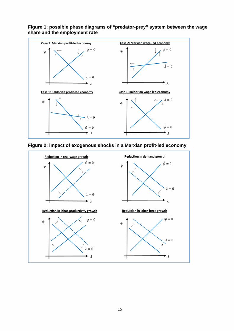
Phases diagrams and cyclical fluctuations

From a mathematical perspective, our 2x2 dynamical model has four possible cases that display counter-clockwise fluctuations on the employment vs wage share plane.15 Figure 1 shows the four phase diagrams and it is worthy to analyze each theoretical possibility in separate.

FIGURE 1 HERE

First, the economy can exhibit Goodwin’s predator-prey dynamics with a Marxian distributive regime and a profit-led employment regime. This case is also locally stable by definition and we will use it as a reference to analyze the US economy in the next section. The economic meaning of this case is that both the rate of employment and income distribution show reversion to the mean, probably driven by macroeconomic policy, which makes the system stable around the steady state.

Second, a Marxian wage-led economy can also show counterclockwise fluctuations of the employment and the wage share. The rate of employment shows unstable dynamics in isolation in this case, but the dynamics of the wage share can neutralize this and produce local stability around the steady state.16 One of the conditions for stability is that the slope of the distribution curve is greater than the slope of the employment curve in this case.17

Third, a Kaldorian profit-led economy can also show counterclockwise and stable dynamics of the employment rate and the wage share of income. Again, one of the conditions for stability is that the slope of the distribution curve is greater than the slope of the employment curve. In this case, it is the wage share that shows explosive dynamics in isolation, but the stability of the rate of employment can make the system locally stable.

Finally, a Kaldorian wage-led economy can show predator-prey dynamics between the wage share and the employment rate, as long as both variables are unstable in isolation. This case is also unstable by definition. In other words, even in face of a small shock, the fluctuations in employment and income distribution spiral out of control, until the system reaches one of the three types of equilibrium mentioned earlier, or “extinction”, with zero employment and zero wage share.18

Let us now analyze the exogenous shocks that can move the steady state of our system. To keep things simple, we will represent this by changes in the intercept of

unemployment would be the predator of the “good” wage share, for those who like morality plays. We will

proceed with the rate of employment because this simplifies the math. 15

For the system to have predator-prey fluctuations, the off-diagonal entries of its Jacobian matrix must have

opposite signs. This leaves the signs of the two diagonal entries open for definition, hence four possible cases. 16

The Jacobian can still have a negative trace. 17

The Jacobian must have a positive determinant. 18

For an example of nonlinearities and multiple equilibrium in a similar model, see Nikiforos and Foley (2012).

9

each reaction function of our model in a Marxian profit-led economy, which seems to be the predominant structure in advanced economies.

Exogenous shocks and comparative statics

From our previous assumptions, exogenous shocks can come from four sources: the real wage (�.), aggregate demand (0.), labor productivity (�.) and demography (8.). Figure 2 shows the impact of negative shocks coming from these four sources and it is worthy to comment on each case separately.

FIGURE 2 HERE

Starting with the real wage, consider an exogenous reduction in �. due to say, lower trade barriers to imports coming from low-wage countries, no adjustment of the minimum wage in face of inflation, a reduction in unionization or any other institutional change that reduces the bargaining power of workers for any given values of the wage share and the rate of employment. This kind of shock moves the distribution curve down in a Marxian profit-led economy, which in its turn means a reduction in the wage share of income and an increase in the rate of employment.

Next, consider an exogenous reduction in the growth rate of aggregate demand due to, say, a major financial crisis that reduces credit expansion and pushes consumption down as most families have to reduce their debt-income ratios. This kind of shock moves the employment curve down in a Marxian profit-led economy, which in its turn results in lower wage share and a lower rate of employment.

Third, consider a reduction in the growth rate of labor productivity because of, say, an exogenous increase in the price of energy that reduces the valued added per unit of labor. This shock moves both the employment and distribution curves up in a Marxian profit-led economy, which in its turn means a higher wage share. The rate of employment may either go up or down, depending on the magnitude of the shock on each curve.

Finally, consider a deceleration of the labor force due to, say, the end of the demographic effects of a baby boom in the past. This shock has the same effect of an exogenous increase in aggregate demand growth, that is, it shifts the employment curve up and raises both the wage share and the rate of employment.

As we will see next, the US economy experienced all of the above shocks in recent decades, plus some other types of shocks.

Employment and income distribution in the US

Figure 3 shows the US data on employment and income distribution since the late 1940s. The wage share is the compensation of employees in % of the net domestic income at production prices.19 The rate of employment is the ratio of civilian employment to the civilian labor force.20 The two series are stationary under the usual statistical tests, provided that we control for structural breaks, which are many.

19

From table 1.10 of the NIPA, published by the US Bureau of Economic Analysis. 20

From series LNS14000000, published by the US Bureau of Labor Statistics.

10

For example, consider the wage share. A visual analysis indicates four probable breaks. First, the wage share jumped up during the Korean War, in 1951-53, and remained at such level until the mid-1960s. Second, the escalation of the Vietnam War and Lyndon Johnson’s “War on Poverty” coincided with another upward jump in the wage share, in the late 1960s. After this, the wage share fluctuated around a relatively stable plateau until the mid-1990s, when Bill Clinton’s welfare reform and the acceleration of labor productivity pulled by information technology raised the profit share of income. Finally, the financial crash of 2008 resulted in a temporary but substantial increase in the wage share, since profits plummeted, but its long-run impact appears to be another downward shift in the wage share.

Moving to employment, the Korean War does not seem to have had a structural impact on the US employment rate, which fluctuated around 95% from the late 1940s through the late 1960s. After this, there seems to have been three structural changes, which in their turn either lag or coincide with the changes in the wage share mentioned above. More specifically, the long-run rate of employment shifted downwards in the early 1970s and then fluctuated around 93% until the early 1990s. The second possible shock occurred in the mid-1990s, in the wake of the US economic expansion during the Clinton administration, and it pushed the average rate of employment back to 95%. Finally, the financial crash of 2008 was a third and clearly negative shock to employment.

It is too early to know whether the 2008 financial crash is a temporary (pulse) or permanent (level) shock to employment and income distribution in the US economy. As we will see later, the usual statistical tests point to both possibilities, as well as to a slow return of the economy to its new steady state. However, before we present econometric results, it is worthy to see the scatter diagram of the wage share and the employment rate because it clearly reproduces the predator-prey dynamics we proposed in our structuralist-Goodwin model.

Figure 4 presents the scatter diagram for the whole sample period. To facilitate the visual analysis, we plotted the Hodrick-Prescott trends of the wage share and employment rate. The data clearly shows the counter-clockwise fluctuation of employment and income distribution, with the employment rate as the “prey” and the wage share as the “predator”.21 The fluctuations follow the pattern we proposed in our theoretical model, but around a moving steady state.

FIGURE 4 HERE

The econometric model

Based on our structuralist theoretical model, the natural questions are: is the US Marxian or Kaldorian? Wage-led or profit-led? As we saw earlier, there are four possible structural configurations consistent with the counter-clockwise fluctuations displayed by the data, three of which from stationary systems. To check the US case, we estimated a vector-autoregressive (VAR) system for our two state variables. We also introduced dummy variables in the model to test whether or not the data confirm the structural breaks we identified from a visual analysis.

The statistical appendix presents the estimated coefficients of the VAR model. The econometric results for the whole sample period indicate a stationary system, with 21

Or, the unemployment rate as the “predator” and the wage share as the “prey”.

11

a Marxian distribution curve, a profit-led employment curve and some structural breaks. More specifically, we introduced four “level” dummy variables in the model, that is: a permanent change in the intercepts of both equations in 1951, 1967, 1995 and 2009.

The statistical results indicate that, at 2% of statistical significance, there was a positive shock to the US wage share in both 1951 and 1967. The results also indicate a negative shock to the wage share in 1995 and 2009, but only the former is statistically significant at 2%. So, despite the reduction in the wage share in recent years, it will take some time for us to know whether the 2008 financial crash changed the long-run distribution of income in the US.

Moving to employment, the results indicate a positive demand shock in 1967 and a negative one in 2009, both at 2% of statistical significance. The results for the rate of employment also indicate a positive shock in 1951 and a negative one in 1995, but these events are not statistically significant. Altogether, the equation for the rate of employment confirms the intuitive perception that the late 1960s was a period of high demand, and recent years a period of stagnation, in the US economy. We will come back to this point in the conclusion.

In addition to its permanent effects, the 2008 financial crash may also have had temporary, but still important effects in the US economy. To test this, we also introduced a “pulse” dummy variable for the 2008 crisis in our VAR model.22 As expected, the results indicate that the wage share went up, and the employment rate down, in the wake of the financial crash, but only the coefficient for the rate of employment is statistically significant at 2%.

To test the velocity of convergence of the US economy after exogenous shocks, figure 5 presents the impulse-response function of our system to a one standard-deviation shock to either the wage share or the rate of employment. The results indicate that the rate of employment goes down after an exogenous increase in the wage share, as well as that the wage share goes up after an exogenous increase in the rate of employment. These results are characteristic of Marxian profit-led economy and, after the shock, both state variables return to their long-run values after approximately 40 quarters. Most of the adjustment occurs in 5 years, but full adjustment takes approximately 10 years.

FIGURE 5 HERE

Finally, to calculate the slopes of the distribution and employment curves of the US economy, we used the steady state of the VAR model for the most recent period. The estimated coefficients indicate a long-run employment rate of 93.4% and a wage share of 67.9%. The distribution and employment “curves” in discrete time are

� = 13.86 + 0.58, (14)

and

� = 136.80 − 0.74,, (15)

respectively. Figure 6 plots the two curves for the relevant interval of the wage share and employment rate.

22

This variable equals one in the last quarter of 2008 and first quarter of 2009.

12

FIGURE 6 HERE

From our econometric results, we can conclude that the wage share was a stationary variable in the US during the period under analysis, but subject to cyclical fluctuations, around a moving steady state. With this view in mind, we can now go back to Piketty’s (2013) proposition on the functional distribution of income

8 – Conclusion

Pikkety’s (2013) theoretical hypotheses about the functional distribution of income are the weakest part of an otherwise landmark book. On one side, organizing the discussion just in terms of the elasticity of substitution combines too many forces in one residual parameter. As we saw in our structuralist model, the functional distribution of income can change, temporarily or permanently, because of institutional and demand shocks not related to technology. This critique does not means that Piketty’s approach to the functional distribution of income is wrong, but actually that it is too aggregated and unrealistic, as usual in mainstream growth theory.

On the other side, Piketty’s proposal that there is no natural tendency for the functional distribution of income to be stable is an empirical hypothesis that, so far, has not been confirmed by the data. Black swans do exist and, maybe, the world economy has entered in a regressive spiral of income concentration and secular stagnation that many economists have feared, many times, in the past. Despite this possibility, our simple structuralist model shows that, at least in the US, the wage share of income shows cyclical fluctuations around a moving steady state, with a long period of convergence. In fact, the adjustment is so slow that, given a sequence of exogenous shocks, the economy is likely to be hit by another shock before it completes its adjustment to the previous one.

The evolution of the US economy since the late 1940s also shows that the wage share tends to fluctuate between 64% and 74% of net domestic factor income, and the civilian employment rate between 90% and 97%. In addition to this, most of the evolution of income distribution and employment in the US can be related to the adjustment of the economy to major exogenous shocks, as wars, new distribution policies (pro-poor in the 1960s and pro-rich in the 1980s) and, yes, changes in the aggregate technology of production. The later also includes trade liberalization and composition effects, which alters labor-productivity growth.

From our structuralist perspective, the US evidence does not confirm that the functional distribution of income is unstable. This means that the elasticity of substitution of capital for labor is equal to one in the long run, but this is not the relevant question. The relevant question is what makes the elasticity of substitution equal to one and, more importantly, at what levels the wage share and the rate of employment tend to stabilize.

Economic policy in general, and macroeconomic policy in particular, plays an important role in determining the steady state of income distribution and employment rates. The fact that the wage share is stable does not mean that it tends to stabilize at a high or adequate level for a democratic regime. It may actually stabilize at a very low level if the major world economies engage in a race to the bottom to gain international competitiveness by reducing their unit labor costs.

13

In fact, since the 2008 financial crash, the world economy has been experiencing a competitive “wage repression”, with too many countries trying to accelerate growth from the supply side without proper attention to fallacies of compositions and the existing space for demand expansion. In this context, Piketty’s (2013) monumental work on capital income and the dangers of rising income inequality is a breath of fresh air, even if it uses traditional tools and problematic assumptions of mainstream economics.

References:

Atkinson, A.B., Piketty, T.and Saez, E. (2011). "Top Incomes in the Long Run of History." Journal of Economic Literature, 49(1): 3-71.

Barbosa-Filho, N.H. (2004). “Simple model of demand-led growth and income distribution.” EconomiA, Selecta, Bras´ılia(DF), v.5, n.3, p.117–154, Dec. 2004.

Barbosa-Filho, N.H. (2014). A structuralist inflation curve. Metroeconomica, 65(2):349–376.

Barbosa-Filho, N.H. and Taylor, L. (2006). “Distributive and demand cycles in the US economy – a structuralis Goodwin Model.” Metroeconomica, Volume 57, Issue 3, pages 389–411, July 2006.

Bhaduri, M., Marglin, S. 1990. Unemployment and the Real Wage: The Economic Basisfor Contesting Political Ideologies. Cambridge Journal of Economics, 14, 375‐393.

Blanchflower, D.G. and Oswald, A.J. (1994), The Wage Curve, Cambridge: The MIT Press.

Dutt, A. (1990). Growth, Distribution and Uneven Development. Cambrigde: Cambridge University Press.

Foley, D. and Michl, T (1997). Growth and Distribution. Cambridge: Harvard University Press.

Goodwin, R. M. (1967). A Growth Cycle. In Socialism, Capitalism, and Growth. Cambridge University Press.

Kalecki, M. (1943). Political aspects of full employment. In Collected Works of Michal Kalecki: Capitalism, Business Cycles and Full Employment. Clarendon Press.

Kiefer, D. and Rada, C. (2013), “Profit maximizing goes global: the race to the bottom”, Working Paper No: 2013-05, Department of Economics, University of Utah.

Lucas, R.E. (2004). ”The Industrial Revolution: Past and Future,” The Region (May), Federal Reserve Bank of Minneapolist, pages 5-20.

Marglin, S. (1984). Growth, Distribution and Prices. Cambridge: Cambridge University Press.

Nikiforos, M. and Foley, D. K. (2012). Distribution and capacity utilization: Conceptual issues and empirical evidence. Metroeconomica, 63(1):200–229.

Piketty, T. (2013). Le Capital au XXIe siècle. Paris: Éditions du Seuil.

Roncolato, L. and Kucera, D. (2013). “Structural drivers of productivity and employment growth: a decomposition analysis for 81 countries,” Cambridge Journal of Economics.

14

Rowthorn, R. E. (1980). Capitalism, Conflict and Inflation. London: Lawrence & Wishart.

Skott, P. (1989). Conflict and Effective Demand in Economic Growth. Cambridge: Cambridge University Press.

Taylor, L. (1991). Income Distribution, Inflation and Growth: Lectures on Structuralist Macroeconomic Theory. Cambridge: Harvard University Press.

Taylor, L. (2004). Reconstructing Macroeconomics: Structuralist Proposals and Critiques of the Mainstream. Harvard University Press.

Von Armin, R. and Barrales, J. (2014). “Demand–driven Goodwin cycles with Kaldorian and Kaleckian features,” University of Utah, mimeo.

Von Armin, R., Tavani, D. and De Carvalho, L.B. (2013). “Redistribution in a Neo-Kaleckian Two-country Model,” Metroeconomica, Volume 65, Issue 3, pages 430–459, July 2014

Yellen, J. and Akerlof, G. (1986), Efficiency wage models of the labor market, Cambrigde: Cambridge University Press.

15

Figure 1: possible phase diagrams of “predator-prey ” system between the wage share and the employment rate

Figure 2: impact of exogenous shocks in a Marxian p rofit-led economy

Case 1: Marxian profit-led economy

Case 1: Kaldorian profit-led economy

Case 2: Marxian wage-led economy

Case 1: Kaldorian wage-led economy

Reduction in real-wage growth

Reduction in labor-productivity growth

Reduction in demand growth

Reduction in labor-force growth

16

Figure 3: wage share of net domestic income at prod uction prices and employment rate of the civilian labor force in the US economy, both variables in % points, HP trend is the Hodrick-Prescott trend of the variable.

Source: US BEA and BLS

62

64

66

68

70

72

74

76

50 55 60 65 70 75 80 85 90 95 00 05 10

Wage share HP trend

89

90

91

92

93

94

95

96

97

98

50 55 60 65 70 75 80 85 90 95 00 05 10

Employment rate HP trend

17

Figure 4: scatter diagram of the Hodrick-Prescott t rends of the wage share and employment rate in the US economy, both variables i n % points

Source: author’s estimate

Figure 5: impulse-response function of a VAR model for the quarterly wage share (WSHARE) and employment rate (ERATE) in the US econ omy, both variables in % points

Source: author’s estimate

1948

1949 1950

1951

1952

1953

1954

1955

1956

1957195819591960

1961

19621963 1964

1965

1966

1967

1968

1969

1970

19711972

197319741975

1976

1977

1978

1979

19801981

1982

1983

19841985 1986 1987

1988

1989

1990

1991

1992

1993

1994 1995

1996

19971998

1999

20002001

2002

2003

2004

2005

200620072008

2009

2010

2011

2012

2013

65

66

67

68

69

70

71

72

73

91 92 93 94 95 96 97

Wage

share

Employment rate

-0.4

0.0

0.4

0.8

1.2

5 10 15 20 25 30 35 40

Response of WSHARE to WSHARE

-0.4

0.0

0.4

0.8

1.2

5 10 15 20 25 30 35 40

Response of WSHARE to ERATE

-1.0

-0.5

0.0

0.5

1.0

1.5

2.0

5 10 15 20 25 30 35 40

Response of ERATE to WSHARE

-1.0

-0.5

0.0

0.5

1.0

1.5

2.0

5 10 15 20 25 30 35 40

Response of ERATE to ERATE

Response to Nonfactorized One Unit Innovations ± 2 S.E.

18

Figure 6: US distribution and employment curves in 2013

Source: author’s estimate

64

65

66

67

68

69

70

71

90 91 92 93 94 95 96 97 98

Employment curve

Distribution curve

Wage share

Employment rate

19

Appendix: the VAR model

We estimated the VAR model with six lags based on the information criteria of models with one through eight lags. Table 1 below shows the estimated coefficients and their corresponding t-Statistics, in brackets. For the coefficients on the dummy variables, * means statistical significance at 2%. The model explains 96% and 98% of the variance of the wage share and employment rate, respectively.

Table 1: VAR model for the US economy in 1949-2013 (258 quarterly observations)

Explaining variable Wage-share

equation

Employment-rate

equation

Wage share (t-1) 0.859289 -0.139979

t statistic [ 13.0038] [-3.50670]

Wage share (t-2) 0.05807 -0.058958

t statistic [ 0.68448] [-1.15042]

Wage share (t-3) 0.143253 0.072419

t statistic [ 1.73389] [ 1.45102]

Wage share (t-4) -0.074987 0.038186

t statistic [-0.90003] [ 0.75873]

Wage share (t-5) -0.196587 0.109141

t statistic [-2.36714] [ 2.17552]

Wage share (t-6) 0.096255 -0.128295

t statistic [ 1.55859] [-3.43895]

Employment rate (t-1) -0.046878 1.440519

t statistic [-0.44338] [ 22.5543]

Employment rate (t-2) 0.249375 -0.590371

t statistic [ 1.33111] [-5.21665]

Employment rate (t-3) -0.189049 0.093601

t statistic [-0.95852] [ 0.78563]

Employment rate (t-4) 0.344182 -0.139524

t statistic [ 1.75184] [-1.17561]

Employment rate (t-5) -0.576759 0.198923

t statistic [-3.13002] [ 1.78708]

Employment rate (t-6) 0.285529 -0.082445

t statistic [ 2.91061] [-1.39126]

Constant 1.011922 14.73489

t statistic [ 0.24258] [ 5.84748]

Level dummy for 1951 0.572636* 0.171376

t statistic [ 2.46572] [ 1.22158]

Level dummy for 1967 0.492996* 0.270242*

t statistic [ 3.48746] [ 3.16464]

Level dummy for 1995 -0.285403* -0.087623

t statistic [-3.09401] [-1.57250]

Level dummy for 2009 -0.202201 -0.385179*

t statistic [-1.25230] [-3.94909]

Pulse dummy for 2008-09 0.22262 -0.56799*

t statistic [ 0.69907] [-2.95259]

2

Rio de Janeiro Rua Barão de Itambi, 60 22231-000 - Rio de Janeiro – RJ São Paulo Av. Paulista, 548 - 6º andar 01310-000 - São Paulo – SP

www.fgv.br/ibre