Elasticity Management of Streaming Data AnalyticsFlows on Clouds

Alireza Khoshkbarforoushhaa,b,∗, Alireza Khosravianc, Rajiv Ranjand

aResearch School of Computer Science, The Australian National University, Canberra ACT0200, Australia

bData61, CSIRO, Canberra ACT 0200, AustraliacSchool of Computer Science, University of Adelaide, Adelaide SA 5005, Australia

dSchool of Computing Science, Newcastle University, Newcastle upon Tyne, United Kingdom

Abstract

A typical Streaming Data Analytics Flow (SDAF) consists of three layers:

data ingestion, analytics, and storage, each of which is provided by a data

processing platform. Despite numerous related studies, we still lack effective

resource management techniques across an SDAF, leaving users struggling with

a key question of: ”What share of different resources (e.g. queue partitions,

compute servers, NoSQL throughputs capacity) does each layer need to operate,

given the budget constraints?”. Moreover, unpredictability of streaming data

arrival patterns coupled with different resource granularity across an SDAF

leads to the following question: ”How would we cope with the variable resource

requirements across the layers for handling variation in volume and velocity of

the streaming data flow?”

This paper introduces a framework that answers the above questions by

employing advanced techniques in control and optimization theory. Specifically,

we present a method for designing adaptive controllers tailored to the data

ingestion, analytics, and storage layers that continuously detect and self-adapt

to workload changes for meeting users’ service level objectives. Our experiments,

based on a real-world SDAF, show that the proposed control scheme is able

∗Corresponding AuthorEmail addresses: a.khoshkbarforoushha@anu.edu.au (Alireza Khoshkbarforoushha),

alireza.khosravianhemami@adelaide.edu.au (Alireza Khosravian), raj.ranjan@ncl.ac.uk(Rajiv Ranjan)

Preprint submitted to Journal of Computer and System Sciences November 11, 2016

to reduce the deviation from desired utilization by up to 48% while improving

throughput by up to 55% compared to fixed-gain and quasi-adaptive controllers.

Keywords: Data analytics flow, Control theory, Data-intensive workloads,

Resource management, Public clouds, Multi-objective optimization

1. Introduction

Growing attention to data-driven enterprises and getting real-time insights

into streaming data leads to the formation of many complex Streaming Data

Analytics Flows (SDAF). For example, online retail companies need to analyse

real-time click stream data and up-to-the minute inventory status for offering5

dynamically priced and customized product bundles. More importantly, cities

are evolving into smart cities by fusing and analyzing data from several stream-

ing sources in real-time. By analyzing data using streaming analytics flows,

real-time situational awareness can be developed for handling events such as

natural disasters, traffic congestion, or major traffic incidents[1].10

A cloud-hosted SDAF typically consists of three layers: data ingestion, an-

alytics, and storage [2, 3]. The data ingestion layer accepts data from multiple

sources such as online services or back-end system logs. The data analytics layer

consists of many platforms including stream/batch processing systems, and scal-

able machine learning frameworks that ease implementation of data analytics15

use-cases such as collaborative filtering and sentiment analysis. The ingestion

and analytics layers make use of different databases during execution and where

required persist the data in the storage layer.

1.1. Research Motivation and Challenges

An SDAF is formed via orchestration [5] of different data processing plat-20

forms across a network of unlimited computing and storage resources. For exam-

ple, Fig. 1 shows the Amazon reference SDAF1 that performs real-time sliding-

1https://github.com/awslabs/aws-big-data-blog/tree/master/aws-blog-kinesis-storm-

clickstream-app

2

Figure 1: A data analytics flow that performs real-time sliding-windows analysis over click

stream data[4].

windows analysis over click stream data. In this architecture, Kinesis acts as a

high-throughput distributed messaging system, Apache Storm2 as a distributed

real-time computation system, and ElastiCache3 as a persistent storage.25

Despite straightforward orchestration, elasticity management of the estab-

lished flow has unique challenges (see 1.1) because it needs to cover three aspects:

i) scalability, the ability to sustain workload fluctuations, ii) cost efficiency,

acquiring only the required resources, iii) time efficiency, resources should be

acquired and released as soon as possible[6, 7, 8].30

Recent studies in elasticity management [9] lack a holistic view of the prob-

lem of resource requirements management (e.g. Compute servers, Cache nodes)

of workloads, whereas [10] showed that the ability to scale down both web servers

and cache tier leads to 65% saving of the peak operational cost, compared to

45% if we only consider resizing the web server tier. This leads us to the first35

research problem: How much resource capacity should be allocated to different

big data platforms within an SDAF such that Service Level Objectives (SLO)

are continuously met? There are two challenges in response to this question:

Workload Dependencies. In an SDAF, workloads pertaining to different plat-

forms are dependent on each other, for example, changes in data velocity at the40

data ingestion layer lead to changes in CPU utilization at the data analytics

layer. Fig. 2 clearly shows how the workload dynamics in the data injection

layer can be traced down to the analytics layer, since the input records in inges-

2http://storm.incubator.apache.org3http://aws.amazon.com/elasticache

3

0 50 100 150 200 250 300 350 400 450 500 5500

2

4

6

xm104

Inpu

tmRec

ords

mSU)

IngestionmLayermSKinesis)

0 50 100 150 200 250 300 350 400 450 500 5500

10

20

30

TimemSmin)

CP

USA

)

AnalyticsmLayermSApachemStorm)

Figure 2: The data arrival rate at the ingestion layer (Amazon Kinesis in Fig.1) is strongly

correlated (coefficient = 0.95) with the CPU load at the analytics layer (Apache Storm)

tion layer strongly correlated with CPU usage in the analytics layer. To provide

smooth elasticity management, these dependencies need to be detected dynam-45

ically. Existing approaches perform resource allocation across different layers

irrespective of inter-layer workload dependencies which make them incapable of

ensuring SLOs for emerging classes of SDAFs.

Different Cloud Services and Monetary Schemes. An SDAF is built upon

multiple big data processing platforms and hardware resources offered by public50

clouds [11] [12] that adopt multiple pricing schemes [13]. For example, Amazon

Kinesis’s4 pricing is based on two dimensions including shard hour 5 and PUT

Payload unit, whereas ElastiCache has one hourly pricing scheme which is based

on the cache node type. To meet the SLOs (e.g. budget constraint) for a data

analytics flow, resource requirements and their associated cost dimensions have55

to be considered during the allocation process.

Once the resource shares are determined, adaptive and timely provisioning of

the resources is yet another issue which forms the second key research problem of

this paper: How can we sustain resource requirements of the SDAF in a timely

4http://aws.amazon.com/kinesis5In Kinesis, a stream is composed of one or more shards, each provides a fixed unit of

capacity.

4

manner? In this regard, we face the following challenge:60

Uncertain Stream Arrival Patterns. Variability of the streaming data ar-

rival rates and their distribution models creates changing resource consumption

in data stream processing workloads [14]. Moreover, forecasting data arrival

patterns is challenging unless the data arrival rates follow some seasonal or pe-

riodical pattern. Therefore, we need an approach that can adjust to the changes65

very quickly while it keeps memory of elasticity decisions made from the near

past.

1.2. Our Approach

To address the first research problem, an advanced technique from operations

research is applied that helps in computing optimal resource allocation decisions70

in a principled and tractable fashion. To do so, we mathematically formulate

the problem of finding the best resource shares across an analytics flow as a

multiple criteria decision making problem in which optimal decisions need to be

taken in the presence of trade-offs between multiple conflicting objectives.

In response to the second research problem, we use advanced control theo-75

retic techniques. Previous studies [15, 16, 17, 18, 19, 20, 21] have shown clear

benefits of using controllers in resource management problems against workload

dynamics. However, we present the first attempt at applying adaptive con-

trollers for elasticity management of multi-layered SDAF that integrates multi-

ple big data processing platforms and cloud-based infrastructure services (e.g.80

VMs [22], provisioned read/write throughput of the tables). Our controller is

equipped with the novel feature of having memory of recent controller decisions

which leads to rapid elasticity [8] of the flow in response to workload dynamics.

1.3. Contributions

In summary, we make the following contributions:85

• To the best of our knowledge, this is the first work that investigates the

problem of multi-layered and holistic resource allocation of an SDAF de-

ployed on public clouds. One of the core contributions of our work is

5

meticulous dependency analysis of the workloads along with the math-

ematical formulation of the problem as per the typical data ingestion,90

analytics, and storage layers of a data analytics flow (Section 3.2).

• We devise controllers individually tailored to the data ingestion, analytics,

and storage layers that are able to continuously detect and self-adapt to

time-varying workloads. A key contribution of the paper here is to pro-

pose a framework for design and asymptotic stability analysis of adaptive95

controllers by employing tools from classic nonlinear control theory. We

also put forward the claim that this study is the first in automated control

of SDAF on clouds (Sections 3.3 and 4).

• With numerous experiments on a real-world click-stream SDAF, we vali-

date the efficiency of our techniques in elasticity management of a complex100

analytics flow under stringent SLO. We also show that, compared to the

state of the art techniques, our approach is able to reduce the RMSE error

(i.e. deviation from desired utilization) by up to 48% while increasing the

throughput by up to 55% (Section 5).

1.4. Organization of the paper105

The rest of the paper is organized as follows: related work is reviewed in

the next section. Section 3.1 provides an overview of the proposed solution.

Section 3.2 is devoted to the analysis of resource shares. In Section 3.3, we

provide a generic adaptive elasticity control scheme and analyse its stability.

Section 4 explains the design principles mandated by practical requirements of110

each layer of an SDAF, enabling effective employment of the proposed adaptive

controller described in Section 3.3 along with the optimal resource allocation

scheme outlined in Section 3.2 to design a complete SDAF resource management

system. Experimental results are given in Section 5 and the concluding remarks

in Section 6 complete the paper.115

6

2. Related Work

This section describes the related work in two broad categories: stream data

processing and elasticity management.

2.1. Stream Data Processing

Stonebraker et al. [23] outlined eight requirements of a real-time stream120

processing system such as guaranteeing data safety and availability, scaling ap-

plications automatically, processing and responding instantaneously, etc. that

are somewhat supported by today’s stream processing systems. Having said

that, emerging complex streaming data analytics flows which bring many plat-

forms and technologies together entail revisiting and enhancing the features125

underpinning the requirements.

One of the key problems in streaming data analytics flows is to ensure end-

to-end security as the medium of communication is untrusted. Nehme et al.

[24] initially proposed the requirement of security in data stream environments,

and they broadly divide the security issues into data-side and query-side secu-130

rity policies. The data-side security preferences are expressed via data security

punctuations and the query-side access privileges are described by query secu-

rity punctuations. The authors extensively work on access control by focusing

on both query security punctuations in their papers [24, 25]. More recently,

Puthal et al. [26, 27] proposed solutions i.e. Dynamic Prime Number Based135

Security Verification and Dynamic Key Length Based Security Framework, to

protect big data streams from external and internal adversaries.

When it comes to scalability features, almost all of the recent stream pro-

cessing systems have the capability to distribute processing across multiple pro-

cessors and machines to achieve incremental scalability. However, adaptive and140

optimized provisioning of various cloud resources for different processing tasks

across an SDAF has been neglected.

7

2.2. Elasticity Management

Elasticity and auto-scaling techniques have been studied extensively in re-

cent years [9][28]. Different techniques such as control theory [15], Queueing145

theory [29], fuzzy logic [30], Markov decision process [31] have been applied to

tackle the problem with respect to different resource types such as Cache servers

[32], HDFS storage [33], or VMs [34]. However, recent studies in resource man-

agement using control theory have clearly shown benefits of dynamic resource

allocations against fluctuating workloads. More importantly, what makes the150

control theory approach stand out in workload management techniques is the

fact that they do not rely on any prior information about the workload behavior

and they impose very mild assumptions on the system model (e.g. as in queue-

ing model). Such features lead to a simple yet effective approach that would

sustain any workload’s shape and dynamics.155

A number of inquiries [15, 33, 35, 36, 16, 17, 37, 18, 19, 20, 21] have

been made into the elasticity management of either data-intensive systems or

single/multi-tier web applications using control theory. Lama et al. in [16]

propose a fuzzy controller for efficient server provisioning on multi-tier clusters

which bounds the 90th-percentile response time of requests flowing through the160

multi-tier architecture. They further improve their approach in [17] by adding

neural networks to the controller in order to avoid tuning the parameters on a

manual trial-and-error basis, and come up with a more effective model in the

face of highly dynamic workloads. Similar to this study, Jamshidi et al. in

[35] propose a fuzzy controller that enables qualitative specification of elasticity165

rules for cloud-based software. They further equipped their technique in [36]

with the Q-Learning technique, a model-free reinforcement learning strategy, to

free users of most tuning parameters. More recently, Farokhi et al. in [37] use

a fuzzy controller for vertical elasticity of both CPU and memory to meet the

performance objective of an application.170

In [33], the authors proposed a fixed-gain controller for elasticity manage-

ment of a Hadoop Distributed File System (HDFS) [38] under dynamic web 2.0

workloads. To avoid oscillatory behavior of the controller, [33] develops a pro-

8

portional thresholding technique which in fact works by dynamically configur-

ing the range for the controller variables. Similarly, in [18], the authors propose175

a multi-model controller which in fact integrates decisions from the empirical

model and workload forecast model with the classical fixed-gain controller. The

empirical model is to retrieve distinct configurations which are capable of sus-

taining the anticipated Quality of Service (QoS) based on recorded data from

the past. In contrast, the forecast model which is built by Fourier Transfor-180

mation is to provide proactive resource resizing decisions for specific classes of

workloads.

More closely related to the topic of this paper, the authors in [20] propose a

resource controller for multi-tier web applications. The proposed control system

is built upon a black-box system modelling approach to alleviate the absence185

of first principle models for complex multi-tier enterprise applications. Unlike

[20], the authors of [15] modeled the system (i.e. web server) as a second-order

differential equation. However, the estimated system model used for control

would become inaccurate if the real workload range were to deviate signifi-

cantly from those used for developing the performance model. The authors of190

[20] next in [21] enhanced the previous work by employing multi-input multi-

output (MIMO) control combined with a model estimator that captures the

relationship between resource allocations and performance in order to assign

the right amount of resource. The resource allocation system can then auto-

matically adapt to workload changes in a shared virtualized infrastructure to195

achieve the average response time. Along similar lines, the authors in [19] in-

corporate a Kalman filter into a feedback controller to dynamically allocate

CPU resources to virtual machines hosting server applications. However, our

work differs in that our control system, rather than adjusting CPU allocation in

a shared infrastructure, which commercial cloud providers do not provide, reg-200

ulates resources in a higher abstraction level that is the number of instantiated

VMs, for example. Above all, unlike our work, this class of control systems are

only quasi-adaptive as their gain parameters do not rely on the history of the

previously computed control gains and hence are unable to dynamically adapt

9

to workload changes (see Section 3.3.2).205

In summary, almost all of the above studies share the same constraint: lack

of a holistic view on resource requirement management in which they have

primarily investigated virtual server allocation problems even in a multi-tier

Internet service. Our work completes this picture through studying different

cloud resources including distributed messaging queue partitions (data ingestion210

layer), VMs (data analytics layer), and provisioned read or write throughputs

of tables (data storage layer).

3. Proposed Solution

In this section we first provide an overview of the proposed solution and then

we will discuss in detail its main components.215

3.1. Solution Overview

Fig. 3 shows the main building blocks of our solution along with the architec-

ture of our testbed which is a real-world SDAF - Click-Stream Analaytics. Our

testbed is similar to Amazon’s reference architecture as shown and discussed

in Fig. 1 except ElasticCache is replaced with DynamoDB, a managed NoSQL220

database service, for seamless scalability. In this SDAF, Kinesis is used for

managing the ingestion of streaming data (e.g. simulated URLs and referrers)

at scale. Apache Storm processes streaming data and persists the aggregated

counters (i.e. number of visitors) in DynamoDB. We discuss further the design

principles followed in building our testbed in Section 4.225

In a nutshell, the workflow of the solution is as follows: First, dependencies

between workloads’ critical resource usage measures such as Kinesis shard uti-

lization, Storm Cluster CPU usage, DynamoDB consumed read/write units are

analysed. To this end, we apply linear regression techniques to the collected

runtime and historical resource profiles to estimate the relationships among230

variables. The dependency information along with the cloud services costs and

the user’s SLO (e.g. budget constraint) constitute the required inputs for the

generation and then search of provisioning plan space.

10

Figure 3: The proposed solution for managing heterogeneous workloads of the SDAF on

Clouds.

The framework resource analyser is capable of determining the maximum

resource shares of each layer in terms of the user’s budget constraint. Due to235

the multi-objective nature of the problem, there usually exist multiple feasible

solutions; which one is best suited to the problem in practice must be identified

either manually or randomly by the system.

Once the upper bound resource shares for each layer are identified, the adap-

tive controller tailored to each of the three layers automatically adjusts resource240

allocations of that layer. This means that the controllers can now freely operate

within the limits of each layer resource. Note that the resource shares can be

determined with respect to arbitrary time windows.

The controllers are regulated based on a number of parameters including

monitored resource utilization value, desired resource utilization value, history of245

the controller’s decisions. In other words, the controllers continuously provision

the resources to adequately serve the incoming records in order to keep resource

utilization of each layer within the specified desired value. Note that for the

sake of simplicity, the sensor and resource actuator as the key components of

any controller-based elasticity management frameworks have not been depicted250

in Fig. 3. In our implementation the sensor module has been built on top of

11

CloudWatch 6 and is responsible for providing recorded resource usage measures

as per the specified monitoring window. The actuator is capable of executing

the controllers’ commands such as adding/removing VMs, increasing/decreasing

number of shards, and the like.255

3.2. Resource Share Analysis

Having an efficient elasticity plan for an SDAF is challenging due to i) the

diversity of cloud resources (e.g. number of Shards in Kinesis, number of VMs

in Storm cluster) used to serve the flow, ii) different pricing schemes of cloud

services, and iii) the dependency between workloads that altogether provide a260

complex provisioning plan space. This space can be of any shape in terms of

SLOs, as such we formulate the goal as:

”Given the budget and estimated dependencies between workloads, what would

be the maximum share of resources for each layer in a data analytics flow?”

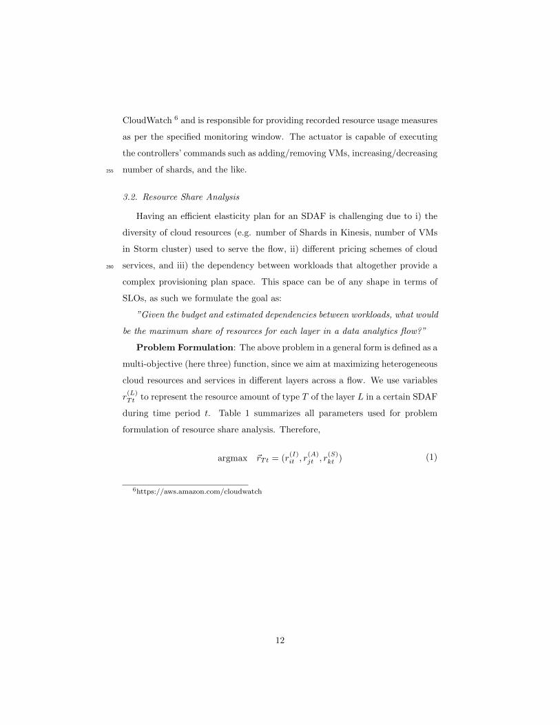
Problem Formulation: The above problem in a general form is defined as a

multi-objective (here three) function, since we aim at maximizing heterogeneous

cloud resources and services in different layers across a flow. We use variables

r(L)Tt to represent the resource amount of type T of the layer L in a certain SDAF

during time period t. Table 1 summarizes all parameters used for problem

formulation of resource share analysis. Therefore,

argmax ~rTt = (r(I)it , r

(A)jt , r

(S)kt ) (1)

6https://aws.amazon.com/cloudwatch

12

Table 1: List of key notations used in this paper.

Parameter Description

L = {I, A, S} L set of the typical SDAF layers including Ingestion (I), An-

alytics (A), and Storage (S)

T = {i, j, k} set of resources of types i, j, or k (e.g. VMs, Queues).

r(L)Tt resource amount of type T of the layer L in a certain streaming

data analytics flow during time period t.

cTd cost of resource type T of dimension d.

Budt specified Budget at time t

Cap(L)Tt the capacity of resource type T at layer L at time t.

a, b, c constant variables obtained via workload dependency analysis.

uk current actuator value. For example, in the analytics layer it

represents the number of VMs allocated to a Storm cluster.

uk+1 new actuator value. It actually represents the next step re-

source allocation amount.

lk the controller gain at time step k.

yk the current sensor measurement. For example, in the analytics

layer it represents the CPU usage measured during the past

monitoring window.

yr the desired reference sensor measurement (i.e. resource uti-

lization) which is specified by the user.

l0, lmax, lmin respectively refer to initial, max, and min gain value.

γ the controller parameter (γ > 0).

13

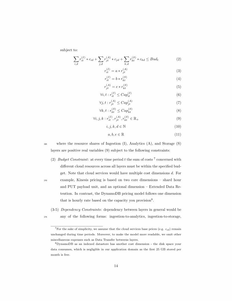
subject to:∑i,d

r(I)it ∗ cid +

∑j,d

r(A)jt ∗ cjd +

∑k,d

r(S)kt ∗ ckd ≤ Budt (2)

r(I)it = a ∗ r(A)

jt (3)

r(I)it = b ∗ r(S)

kt (4)

r(A)jt = e ∗ r(S)

kt (5)

∀i, t : r(I)it ≤ Cap

(I)it (6)

∀j, t : r(A)jt ≤ Cap

(A)jt (7)

∀k, t : r(S)kt ≤ Cap

(S)kt (8)

∀i, j, k : r(I)it , r

(A)jt , r

(S)kt ∈ R+ (9)

i, j, k, d ∈ N (10)

a, b, e ∈ R (11)

where the resource shares of Ingestion (I), Analytics (A), and Storage (S)265

layers are positive real variables (9) subject to the following constraints:

(2) Budget Constraint : at every time period t the sum of costs 7 concerned with

different cloud resources across all layers must be within the specified bud-

get. Note that cloud services would have multiple cost dimensions d. For

example, Kinesis pricing is based on two core dimensions – shard hour270

and PUT payload unit, and an optional dimension – Extended Data Re-

tention. In contrast, the DynamoDB pricing model follows one dimension

that is hourly rate based on the capacity you provision8.

(3-5) Dependency Constraints: dependency between layers in general would be

any of the following forms: ingestion-to-analytics, ingestion-to-storage,275

7For the sake of simplicity, we assume that the cloud services base prices (e.g. cid) remain

unchanged during time periods. Moreover, to make the model more readable, we omit other

miscellaneous expenses such as Data Transfer betweens layers.8DynamoDB as an indexed datastore has another cost dimension - the disk space your

data consumes, which is negligible in our application domain as the first 25 GB stored per

month is free.

14

and analytics-to-storage. These models and in particular their constant

variables including a, b, and e are learned and determined by the linear

regression technique. Note that every flow would not necessarily exhibit

all of these dependencies at a given point of time.

(6-8) Capacity Constraints: at every time period t the calculated resource share280

must be within the cloud service capacity limits9.

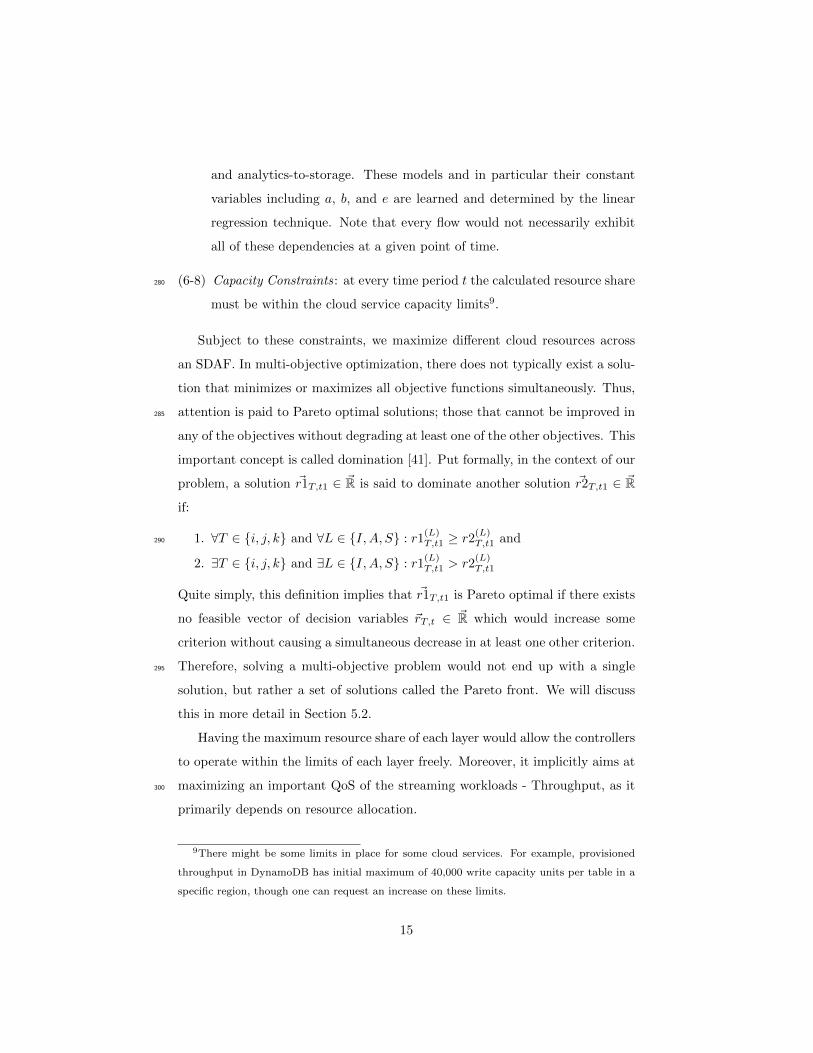
Subject to these constraints, we maximize different cloud resources across

an SDAF. In multi-objective optimization, there does not typically exist a solu-

tion that minimizes or maximizes all objective functions simultaneously. Thus,

attention is paid to Pareto optimal solutions; those that cannot be improved in285

any of the objectives without degrading at least one of the other objectives. This

important concept is called domination [41]. Put formally, in the context of our

problem, a solution ~r1T,t1 ∈ ~R is said to dominate another solution ~r2T,t1 ∈ ~R

if:

1. ∀T ∈ {i, j, k} and ∀L ∈ {I, A, S} : r1(L)T,t1 ≥ r2

(L)T,t1 and290

2. ∃T ∈ {i, j, k} and ∃L ∈ {I, A, S} : r1(L)T,t1 > r2

(L)T,t1

Quite simply, this definition implies that ~r1T,t1 is Pareto optimal if there exists

no feasible vector of decision variables ~rT,t ∈ ~R which would increase some

criterion without causing a simultaneous decrease in at least one other criterion.

Therefore, solving a multi-objective problem would not end up with a single295

solution, but rather a set of solutions called the Pareto front. We will discuss

this in more detail in Section 5.2.

Having the maximum resource share of each layer would allow the controllers

to operate within the limits of each layer freely. Moreover, it implicitly aims at

maximizing an important QoS of the streaming workloads - Throughput, as it300

primarily depends on resource allocation.

9There might be some limits in place for some cloud services. For example, provisioned

throughput in DynamoDB has initial maximum of 40,000 write capacity units per table in a

specific region, though one can request an increase on these limits.

15

3.3. Elasticity Controller

Control theory mandates that a system model that describes the mathe-

matical relationship between the control input and output is specified before a

controller is designed. Few studies in workload management of computer sys-305

tems follow this approach in which the system is modelled, for example, as a

difference equation [15] or using queueing theory. Due to the complexity and

uncertainty of computer systems, obtaining dynamic models describing their

behavior with difference equations requires implementation of comprehensive

system identification techniques. These techniques inevitably increase the com-310

plexity of the control system and may decrease the robustness of the closed

loop system (or even cause instability) if the system configuration or workload

range deviates from those used to estimate the unknown system parameters.

Similarly, in queueing theory every model is built upon a number of assump-

tions such as arrival process that may not be met by certain applications and315

workloads. Building and maintaining these models are complicated even for a

multi-process server model [15], let alone a chain of diverse parallel distributed

platforms, as we have in a complex data analytics flow.

For this reason, most prior work [33, 20, 21, 37, 35, 16, 17] on applying control

theory to computer systems employs a black box approach in which the system320

model is assumed unknown and minimal assumptions are imposed on the system

model that enable stability analysis of the closed-loop system. The downside of

this approach is that it does not provide enough flexibility for proving strong

stability results. In fact, most of the results available in the literature either lack

proper stability analysis or only prove what is known as the internal stability325

(or at most bounded-input-bounded-output stability) in the control literature

[39], implying that the resulting output error (i.e. the difference between the

system output and its desired value) is bounded for all times. Nevertheless, it is

known in the control literature that, in general, the internal stability does not

imply asymptotic (or exponential) stability [39, 40], meaning that the output330

error is not only bounded, but also asymptotically (exponentially) converges to

zero as time passes.

16

𝑢

𝑦

𝑢min 𝑢m𝑎𝑥

𝑦min

𝑦m𝑎𝑥

(a)

𝑢

𝑦

𝑢min 𝑢m𝑎𝑥

𝑦min

𝑦m𝑎𝑥 𝑦 𝑢

𝑦r

System

Controller

?

(b)

Figure 4: a) Input-output linear model, b) Control feedback loop.

Therefore, here we propose a framework for designing controllers for com-

puter systems and analyzing their stability by proposing a static, yet unknown,

model for the underlying systems. Using this framework, we propose a generic335

adaptive controller which requires very minimal information about the system

model parameters. Using tools from classic nonlinear control theory (e.g. Lya-

punov theory), we provide a rigorous stability analysis and prove the asymptotic

(exponential) stability of the resulting closed loop system [42].

3.3.1. A Framework for Controller Design and Stability Analysis340

Denote the input of a system (assigned by the actuator) at the time k by

uk ∈ R and the system output (i.e. the sensor reading) by yk ∈ R. We assume

that the system input and output are related via a static, yet unknown, smooth

function. That is to say yk = f(uk) where f : R → R is a smooth function.

In practice, the smooth function f can be linearized at the operating point.

Hence, we approximate the system model with a linear function (see Fig. 4a).

Nevertheless, we still assume that the parameters of the linear model, i.e. the

slope and the y-intercept, are unknown. That is,

yk = auk + b (12)

17

with unknown a ∈ R and b ∈ R. Note that, a and b generally depend on

the operating point of the system (which itself depends on the workload). We

further assume that an upper bound of the amplitude of a and the sign of a are

known, that is, we know if the output is a decreasing (a < 0) or an increasing

(a > 0) function of the input. These are very mild assumptions on the system345

model that can be easily verified in practice. For instance, increasing the number

of virtual machines (i.e. the system input) in the data analytics layer decreases

the CPU utilization (i.e. the system output or sensor reading)10. Hence, the

corresponding system model for the data analytics layer is decreasing and a < 0

in this case.350

Consider the control feedback loop illustrated in Fig. 4b. The control objec-

tive is to design the control input uk such that the output yk (remains bounded

for all times and) converges to a reference (desired) constant value yr ∈ R as k

goes to infinity.

For the sake of simplicity and without loss of generality, we assume a < 0355

in the remaining parts of the paper. Nevertheless, the theory proposed here is

applicable to the case that a > 0 with straightforward modifications.

3.3.2. A Generic Adaptive Controller

We propose the following adaptive controller.

uk+1 = uk + lk+1(yk − yr), (13)

where the controller gain lk+1 is adaptively updated according to the following

multi criteria update law.

lk+1 =

lk + γ(yk − yr), if lmin ≤ lk + γ(yk − yr) ≤ lmax

lmin, if lk + γ(yk − yr) < lmin

lmax, if lk + γ(yk − yr) > lmax

(14)

10See Section 4.2 for further details on the data analytics layer controller

18

Here, lk is the controller gain at the time k, lmin > 0 and lmax > 0 are the lower

bound and the upper bound of the controller gain11, respectively, and γ > 0 is360

a controller parameter. Table 1 summarizes all parameters used in the adaptive

controller design.

The multi criteria update law (14) ensures that the values of lk are bounded

by lmin and max for all k (the initial controller gain l0 should be chosen such

that lmin ≤ l0 ≤ lmax). The proposed adaptive controller, the constant gain365

controller of [33, 18] and the quasi-adaptive controller of [20] all have the same

standard structure (13). The difference between these three control schemes is

the gain lk+1. In the constant gain controller, the gain lk+1 is simply constant

for all time. In the quasi-adaptive controller, the gain lk+1 is computed as a

predetermined function of the measurements and desired output, however, this370

function is memoryless meaning that the gain lk+1 does not depend on lk which

is computed in the previous step. In contrast, the adaptive update rule (14)

does utilize the previously computed gain lk for computing the new gain lk+1,

thus resulting in a truly adaptive control scheme[42].

In order to analyse the stability of the closed loop system, we define the

output error

ek := yk − yr. (15)

In ideal conditions where the measurements are noise free and the system model375

is accurate, the control goal is achieved if the error ek converges to zero as k

goes to infinity, yielding yk to converge toward the desired output yr.

For stability analysis in the following theorem, we assume that a and b are

constants (in theory). This assumption practically implies that the rate at which

the control value uk is computed is much faster than the speed at which the380

system parameters a and b change. This implies that the update rate of the

controller should be much faster than the rate of change of the workload.

11We later on propose criteria for choosing appropriate lmin and lmax to ensure stability of

the closed loop system.

19

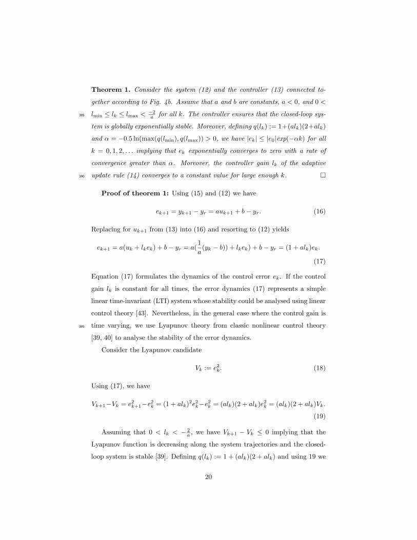
Theorem 1. Consider the system (12) and the controller (13) connected to-

gether according to Fig. 4b. Assume that a and b are constants, a < 0, and 0 <

lmin ≤ lk ≤ lmax <−2a for all k. The controller ensures that the closed-loop sys-385

tem is globally exponentially stable. Moreover, defining q(lk) := 1+(alk)(2+alk)

and α = −0.5 ln(max(q(lmin), q(lmax)) > 0, we have |ek| ≤ |e0|exp(−αk) for all

k = 0, 1, 2, . . . implying that ek exponentially converges to zero with a rate of

convergence greater than α. Moreover, the controller gain lk of the adaptive

update rule (14) converges to a constant value for large enough k. �390

Proof of theorem 1: Using (15) and (12) we have

ek+1 = yk+1 − yr = auk+1 + b− yr. (16)

Replacing for uk+1 from (13) into (16) and resorting to (12) yields

ek+1 = a(uk + lkek) + b− yr = a(1

a(yk − b)) + lkek) + b− yr = (1 + alk)ek.

(17)

Equation (17) formulates the dynamics of the control error ek. If the control

gain lk is constant for all times, the error dynamics (17) represents a simple

linear time-invariant (LTI) system whose stability could be analysed using linear

control theory [43]. Nevertheless, in the general case where the control gain is

time varying, we use Lyapunov theory from classic nonlinear control theory395

[39, 40] to analyse the stability of the error dynamics.

Consider the Lyapunov candidate

Vk := e2k. (18)

Using (17), we have

Vk+1−Vk = e2k+1−e2k = (1 + alk)2e2k−e2k = (alk)(2 + alk)e2k = (alk)(2 + alk)Vk.

(19)

Assuming that 0 < lk < − 2a , we have Vk+1 − Vk ≤ 0 implying that the

Lyapunov function is decreasing along the system trajectories and the closed-

loop system is stable [39]. Defining q(lk) := 1 + (alk)(2 + alk) and using 19 we

20

have Vk+1 = q(lk)Vk which yields

Vk = V0q(lk)q(lk−1) . . . q(l1)q(l0), (20)

for all k = 0, 1, 2, . . .. Since 0 < lmin ≤ lk ≤ lmax < − 2a , it is straightforward to

verify that 0 < q(lk) ≤ qmax < 1 where qmax := max(q(lmin), q(lmax)). Hence,

we have q(lk)q(lk−1) . . . q(l1)q(l0) ≤ qkmax which together with (20) yields

Vk ≤ V0qkmax = V0 exp(− ln(q−1max)k), (21)

which implies that the geometric progression Vk decays exponentially to zero

with a convergence rate greater than 2α = ln(q−1max) > 0. Substituting for Vk

from (21) into (18) and taking the square root of the sides we have

|ek| ≤ |e0|exp(−αk) (22)

which proves the first claim of the theorem.

Next, we proceed to show that the gain lk converges to a constant value

for large enough k, say k = ∞. We know that l∞ is governed by one of the

three criteria of the adaptation law (14). Suppose that lk is governed by the400

first criteria for large k. We use (15) to replace yk − yr with ek in the first

criteria of (14) to obtain lk+1 − lk = γek. Taking the norm of the sides and

recalling (22) we have |lk+1 − lk| ≤ γ|e0|exp(−αk). Hence, for large enough k

we have |lk+1 − lk| ≈ 0 which effectively implies that lk+1 ≈ lk. This means

that lk converges to a constant value if lk is governed by the first criteria for405

large enough k. It remains to be shown that lk converges to a constant value

if it is not completely governed by the first criteria of (14). If l∞ is governed

by the second or the third criteria, we have either l∞ = lmin or l∞ = lmax,

respectively. Since lmin and lmax are both constants, l∞ would be constant in

this case as well. Note that, for large k, lk cannot indefinitely switch between410

the three criteria of (14) as we have already proved that lk+γ(yk−yr), the value

of which determines the criteria of (14), converges to a constant and eventually

satisfies only one of the criteria for large k. This completes the proof.

21

Remark 1. The stability proof of Theorem 1 is provided for a generic time

varying trajectory of control gain lk. Hence, this stability proof is valid not415

only for the proposed adaptive update rule (14), but also for the constant gain

controller (see e.g. [33]) and the quasi-adaptive controller [20] (provided that

those controllers satisfy the gain requirements of theorem 1). For the case of

the fixed gain controller, it can be verified that the requirements of theorem 1

are necessary and sufficient for exponential stability of the closed loop system.420

In this case, theorem 1 provides coherent analytical limits on the gain of the

controller that guarantee the stability of the closed loop system.

3.3.3. Gain Function (lk) Behavior Analysis

One of the key indicators of an effective elasticity technique is the ability to

quickly scale up or down, which is called the elasticity speed [8, 7]. The scale-425

up speed refers to the time it takes to shift from an under-provisioned state to

an optimal or over-provisioned state. Conversely, the scale-down speed refers

to the time it takes to shift from an over-provisioned state to an optimal or

under-provisioned state [7].

We put forward the claim that our adaptive controller, compared to the fixed-430

gain controllers [33, 18] and quasi-adaptive controllers [20, 21], shows higher

elasticity speed as it keeps the history of the controller decisions through up-

dating the gain parameter with respect to the error (see Eq. 14). The bigger

the gain-parameter value (lk+1), the higher the speed of elasticity as per the

standard controller Eq. (13) (also see Eq. (5) in [20] or Eq. (1) in [33]).435

To support our claim, we first explain the normal and extreme scenarios of

workload behaviors:

1. Normal overload/underload : In normal workload behavior, when a system

is over-provisioned, de-scaling of resources leads to higher utilization (yk)

and hence decreases the distance from the desired value (yr). Fig. 5a440

demonstrates this situation where the distance reduces from |−80| (on the

left) to the optimal point that is 0 (on the right). In contrast, when a

system is under-provisioned, scaling of resources again reduces the error

22

(a) Descaling Process (Scenario 1) (b) Scaling Process (Scenario 1)

(c) Descaling Process (Scenario 2) (d) Scaling Process (Scenario 2)

Figure 5: Gain parameter behavior under different load scenarios.

(i.e. yk − yr) as x-axis displays in 5b.

2. Instantaneous massive overload/underload : In contrast to normal work-445

load behavior, in the event of instantaneous massive overload or underload,

scaling or de-scaling of the system does not necessarily decrease the error

for a while. In other words, the system load increases or decreases much

faster than the rate at which the resource manager reacts. Fig. 5c and 5d

show this circumstances where in Fig. 5c the utilization is not improved450

(as we move from |−80| to |−100|) even after de-scaling the resource. Sim-

ilarly, scaling a highly overloaded system does not reduce the error yk−yrand the distance increases from |90| towards |160| as shown in Fig. 5d.

Note that this situation is temporary and the workloads will be back to

a normal situation (Fig. 5a and 5b) sooner or later. Although transient,455

these extreme cases may typically either hit performance severely or lead

to huge resource wastes.

Now we can look into the gain parameter behavior in different scenarios

and compare the elasticity speed of different controllers as shown in Fig. 5.

The gain function of our controller lk+1 = lk + γ(yk − yr) is shown with the460

23

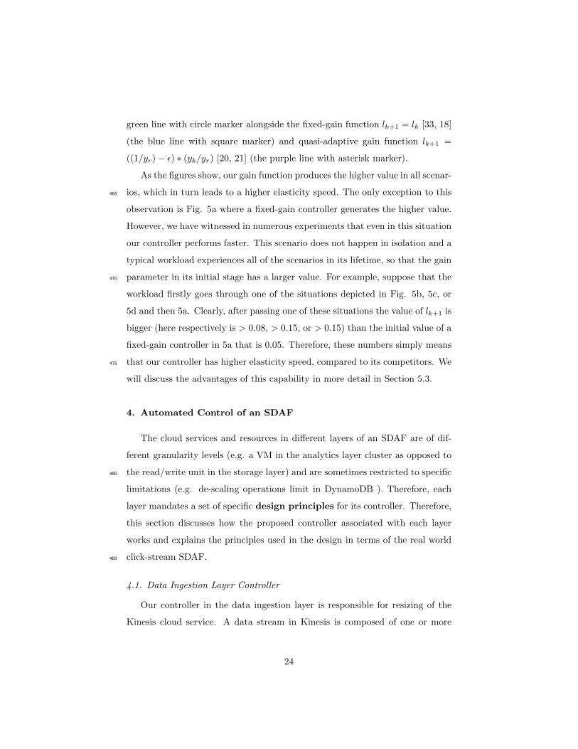
green line with circle marker alongside the fixed-gain function lk+1 = lk [33, 18]

(the blue line with square marker) and quasi-adaptive gain function lk+1 =

((1/yr)− ε) ∗ (yk/yr) [20, 21] (the purple line with asterisk marker).

As the figures show, our gain function produces the higher value in all scenar-

ios, which in turn leads to a higher elasticity speed. The only exception to this465

observation is Fig. 5a where a fixed-gain controller generates the higher value.

However, we have witnessed in numerous experiments that even in this situation

our controller performs faster. This scenario does not happen in isolation and a

typical workload experiences all of the scenarios in its lifetime, so that the gain

parameter in its initial stage has a larger value. For example, suppose that the470

workload firstly goes through one of the situations depicted in Fig. 5b, 5c, or

5d and then 5a. Clearly, after passing one of these situations the value of lk+1 is

bigger (here respectively is > 0.08, > 0.15, or > 0.15) than the initial value of a

fixed-gain controller in 5a that is 0.05. Therefore, these numbers simply means

that our controller has higher elasticity speed, compared to its competitors. We475

will discuss the advantages of this capability in more detail in Section 5.3.

4. Automated Control of an SDAF

The cloud services and resources in different layers of an SDAF are of dif-

ferent granularity levels (e.g. a VM in the analytics layer cluster as opposed to

the read/write unit in the storage layer) and are sometimes restricted to specific480

limitations (e.g. de-scaling operations limit in DynamoDB ). Therefore, each

layer mandates a set of specific design principles for its controller. Therefore,

this section discusses how the proposed controller associated with each layer

works and explains the principles used in the design in terms of the real world

click-stream SDAF.485

4.1. Data Ingestion Layer Controller

Our controller in the data ingestion layer is responsible for resizing of the

Kinesis cloud service. A data stream in Kinesis is composed of one or more

24

shards, each of which provides a fixed unit of capacity12 for persisting incoming

records. Therefore, the data capacity of the stream is a function of the number490

of shards that are specified for the stream. As the data rate increases, more

shards need to be added to scale up the size of the stream. In contrast, shards

can be removed as the data rate decreases.

As mentioned in Section 3.1, each controller is equipped with both sensor and

actuator components. The sensor here continuously reads the incoming records

stream from CloudWatch and calculates the resource utilization as average write

per second:(∑n

i=1 IncomingRecordsi)/(n ∗ 60)

(ShardsCount ∗ 1000)(23)

where n is the number of monitoring time windows in minutes and assuming

each record is less than 1 KB. This measure inputs the controller and it then495

makes the next resource resizing decision as per the logic discussed in Section

3.3.1 and invokes the actuator to execute increaseShards, decreaseShards, or

doNothing commands.

4.2. Data Analytics Layer Controller

The analytics layer controller in the click-stream application is in charge of500

Apache Storm cluster resizing. A Storm cluster consists of the master node and

the worker nodes which are coordinated by Apache ZooKeeper. The master

node is responsible for distributing code around the cluster, assigning tasks to

workers, and monitoring for failures. Each worker node listens for work assigned

to its machine and starts and stops worker processes as necessary based on what505

a master has assigned to it. Each worker process executes a subset of a job called

topology; a running topology consists of many worker processes spread across

many machines. The logic for a realtime application is packaged into a Storm

topology, a graph of stream transformations.

12Each shard supports up to 5 transactions/second for reads, up to a maximum total data

read rate of 2 MB/second and up to 1,000 records/second for writes, up to a maximum total

data write rate of 1 MB/second

25

Our Storm cluster is built on the Amazon EC2 instances whose size is reg-510

ulated by the control system. The sensor here records the CPU utilization of

the cluster in terms of the specified time window. Following that the instances

are acquired or released. However, this process is not instant and it may take

several minutes to start up a VM. During this time, the data flow analytics is

vulnerable to missing the SLOs. In response and to counter this problem, we515

inject a number of already configured worker VMs in the cluster under Stopped

status. In the event of scaling, these pre-configured VMs are added to the cluster

at the earliest opportunity.

To release a worker VM in the event of de-scaling, our actuator finds the

most economical VM to stop. The EC2 instance prices are on an hourly basis.520

As the instances are fired in different time slots, it is more economical to stop

the instance that uses the maximum of its current time slot. Therefore, the

instance that has the least remaining time of the current paid 1 hour slot is the

economical candidate to be stopped. Fig. 6 shows a sample of three VMs with

different uptimes and remaining times where VM 2 and then 1 are respectively525

the most economical VMs to be stopped. We calculate those instances that

show least cost to stop using the following equation:

mini∈n

f(vmi),

f(vmi) = uptimevmimod t

(24)

where uptime refers to the VM uptime and t is the time slot which is on an

hourly basis in AWS 13.

4.3. Data Storage Layer Controller530

DynamoDB sits in our storage layer and is capable of persisting the analytics

results. The controller in this layer is responsible for adjusting the number

of provisioned write capacity units where each unit can handle 1 write per

13In our experiments, the uptime is retrieved from CloudWatch in milliseconds, and hence

the t is set to the value of 1h * 60min * 60sec * 1000millisec.

26

1h

VM 1

VM 2

VM 3

remaining time

uptime

remaining time

remainingtime

Figure 6: VMs are launched at different time slots so that they are of different cost to stop.

Thus, it is more economical to stop a VM with the minimum remaining time.

second. To this end, the sensor retrieves the ConsumedWriteCapacityUnits

from CloudWatch and calculates write utilization per second as a main input

to the control system as follows:

(∑n

i=1 ConsumedWriteCapacityUnits)/(n ∗ 60)

ProvisionedWriteCapacityUnits(25)

where n is the number of monitoring time windows in minutes and assum-

ing items are less than 1 KB in size. This measure inputs the controller and

following that the next resource resizing decision is made and the actuator

is invoked to execute increaseProvisioinedWriteCapacity, decreaseProvisioined-

WriteCapacity, or doNothing commands.535

Cloud services sometimes come with some limitations in the number of scal-

ing or de-scaling operations in a certain period of time. For example, in Dy-

namoDB a user can not decrease the ReadCapacityUnits/WriteCapacityUnits

settings more than four times per table in a single UTC calendar day. This

limitation may lead to reasonably high resource waste in highly fluctuating540

workloads. To address this issue, our controller uses a simple yet effective back-

off strategy. The actuator performs the de-scaling operation only after reaching

the back-off threshold - a number of consecutive de-scaling requests from the

controller. This strategy filters transient behavior of workloads and alleviate

the problem of resource waste.545

27

5. Experimental Results

The purpose of our experiments in this section is to demonstrate that (i)

given the budget and dependency constraints, we are able to efficiently deter-

mine the share of different resources across an SDAF (Section 5.2), (ii) Our

controller outperforms the state of the art fixed-gain and quasi-adaptive con-550

trollers in managing fine-grained cloud resources in dynamic data stream pro-

cessing settings (Section 5.3), and most importantly (iii) our framework is able

to manage elasticity of the SDAF on public clouds (Section 5.4).

5.1. Experimental Setup

We have implemented our framework in Java. To implement the workload555

dependency and resource share analyser, we respectively employed Apache Com-

mons14 and the MOEA framework [44]. We tested our controllers and resource

share analyser against real world click-stream analytics, as shown in Fig. 3.

In the testbed, we used three t2.micro instances as click-stream data pro-

ducers15, each is able to produce up to ∼5K records per seconds. The data560

ingestion and storage, as discussed earlier, are handled by Amazon Kinesis and

DynamoDB services. The Storm cluster is made up of two m4.large instances

for Zookeeper and Storm master node (i.e. Nimbus server in Storm terminology)

and a number of workers (i.e. supervisors) which are either t2.micro, t2.small,

m3.medium, or m4.xlarge.565

5.2. Evaluation Results: Optimized Resource Share Determination

To solve a multi-objective optimization problem and find the Pareto front,

a large number of algorithms exist in the literature [41]. Our framework uses a

nondominated sorting genetic algorithm II (NSGA-II) [45] to search the provi-

sioning plan space.570

14http://commons.apache.org15https://github.com/awslabs/amazon-kinesis-data-visualization-sample

28

The prerequisite of resource share determination is workload dependency

analysis. To illustrate how the framework computes with the resource shares of

each layer, in our testbed the following constraints were evaluated:

1. 5 ∗ r(A)jt1 >= r

(I)it1

2. 2 ∗ r(A)jt1 <= r

(I)it1575

3. 2 ∗ r(I)it1 <= r(S)kt1

where i, j, and k respectively refer to the number of shards in ingestion,

VMs in analytics, and Write Capacity units in storage layer at time t1. More-

over, suppose that the daily budget of running the click-stream analytics flow

on public clouds is $32.25. Given the budget and dependency constraints for-580

mulated in Section 3.2, the algorithm finds the Pareto optimal solutions and its

corresponding frontier surface as displayed in Fig. 7a and 7b.

As we can see, solving the problem ends up with six feasible solutions (see

Fig. 7a), each representing the resource shares of Kinesis, Storm, DynamoDB si-

multaneously. The underlying assumption here is that a solution to the problem585

must be identified by an expert to be implemented in practice. For example, the

DevOps manager of the analytics flow plays an important role as it is expected

to be an expert in the problem domain.

5.3. Evaluation Results: Adaptive Controller Performance

In this section, we report the performance of our controller, compared with590

the state of the art constant gain [33, 18] and quasi-adaptive controllers [20]. Due

to workload fluctuations over time, it is hardly possible to provide a truly-fair

testbed for comparison. Having said that, we modified the testbed to make it

as fair as possible for pair-wise comparison between controllers. To this end, we

conducted the experiments on all layers but analytics, since it is hard to control595

the input to this layer. In other words, as the inputs to Kinesis and DynamoDB

are manageable, we could provide a fair starting point for the systems.

Fig. 8a and 8b denote the architecture of the Kinesis and DynamoDB con-

trollers testbed. In the former, we have created three streams in Amazon Kinesis

29

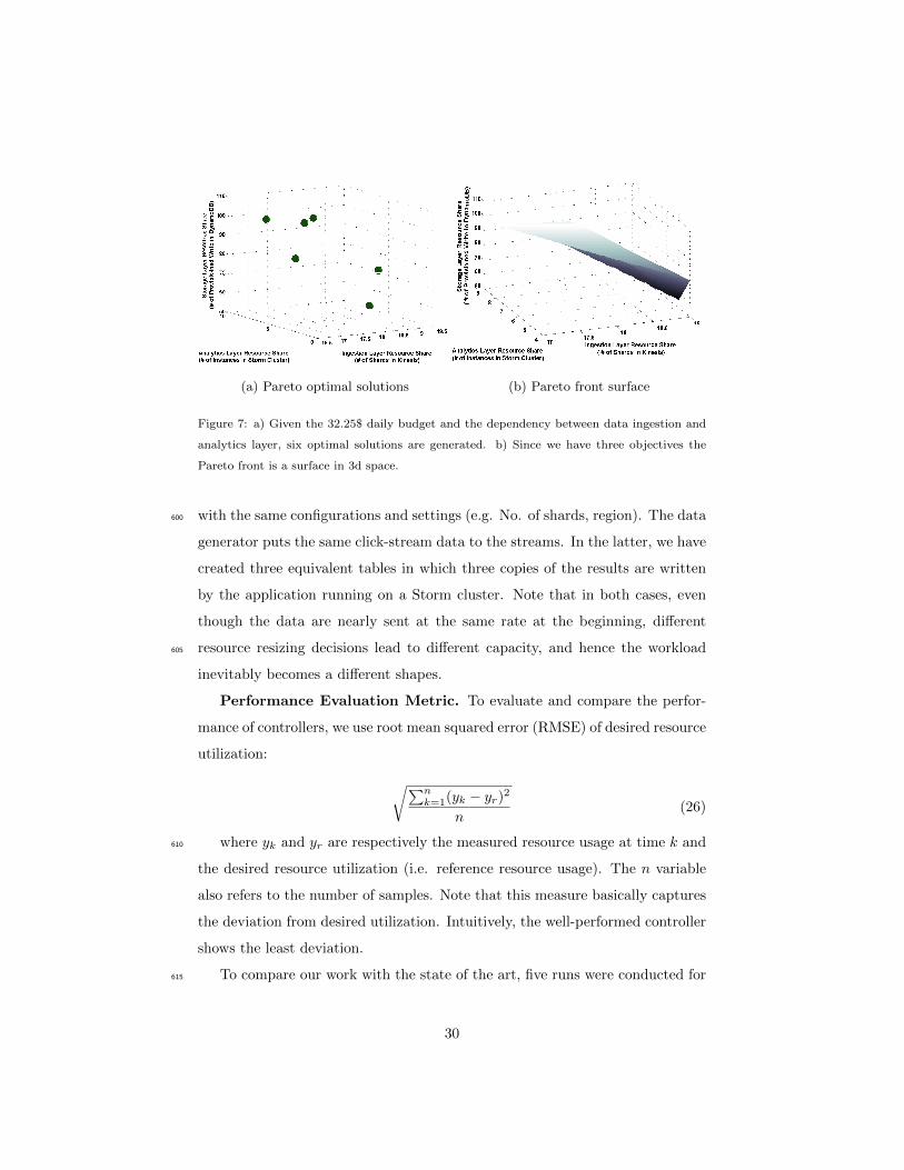
(a) Pareto optimal solutions (b) Pareto front surface

Figure 7: a) Given the 32.25$ daily budget and the dependency between data ingestion and

analytics layer, six optimal solutions are generated. b) Since we have three objectives the

Pareto front is a surface in 3d space.

with the same configurations and settings (e.g. No. of shards, region). The data600

generator puts the same click-stream data to the streams. In the latter, we have

created three equivalent tables in which three copies of the results are written

by the application running on a Storm cluster. Note that in both cases, even

though the data are nearly sent at the same rate at the beginning, different

resource resizing decisions lead to different capacity, and hence the workload605

inevitably becomes a different shapes.

Performance Evaluation Metric. To evaluate and compare the perfor-

mance of controllers, we use root mean squared error (RMSE) of desired resource

utilization:

√∑nk=1(yk − yr)2

n(26)

where yk and yr are respectively the measured resource usage at time k and610

the desired resource utilization (i.e. reference resource usage). The n variable

also refers to the number of samples. Note that this measure basically captures

the deviation from desired utilization. Intuitively, the well-performed controller

shows the least deviation.

To compare our work with the state of the art, five runs were conducted for615

30

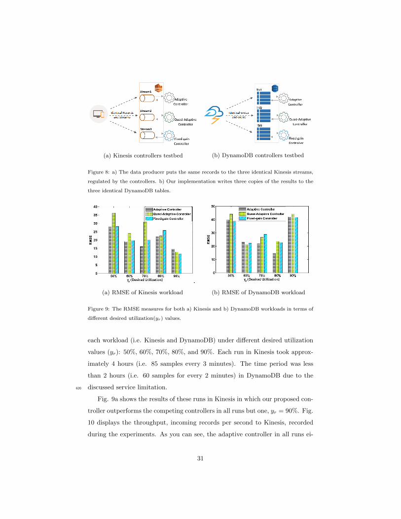
(a) Kinesis controllers testbed (b) DynamoDB controllers testbed

Figure 8: a) The data producer puts the same records to the three identical Kinesis streams,

regulated by the controllers. b) Our implementation writes three copies of the results to the

three identical DynamoDB tables.

(a) RMSE of Kinesis workload (b) RMSE of DynamoDB workload

Figure 9: The RMSE measures for both a) Kinesis and b) DynamoDB workloads in terms of

different desired utilization(yr) values.

each workload (i.e. Kinesis and DynamoDB) under different desired utilization

values (yr): 50%, 60%, 70%, 80%, and 90%. Each run in Kinesis took approx-

imately 4 hours (i.e. 85 samples every 3 minutes). The time period was less

than 2 hours (i.e. 60 samples for every 2 minutes) in DynamoDB due to the

discussed service limitation.620

Fig. 9a shows the results of these runs in Kinesis in which our proposed con-

troller outperforms the competing controllers in all runs but one, yr = 90%. Fig.

10 displays the throughput, incoming records per second to Kinesis, recorded

during the experiments. As you can see, the adaptive controller in all runs ei-

31

Figure 10: Throughput QoS for Kinesis workload.

ther produces comparable throughput (i.e. when yr = 50% or yr = 70%) or625

improves it considerably by up to 55% when yr = 60%.

In the DynamoDB workload, our controller with adaptive gain produces

less error (RMSE) than the quasi-adaptive controller in all but one run when

yr = 60%. When it comes to comparison with the constant gain controller, the

adaptive control system is less successful as it shows higher error rates in 3 out630

of 5 runs (i.e. yr = 50%, 60%, and 90%). This is mainly due to the DynamoDB

de-scaling limitation (as discussed in Section 4.3). The adaptive controller es-

sentially adjusts the gain parameter with respect to the workload dynamics,

whereas the service does not allow more than four de-scaling operations in a

day. To handle that we devised the back-off strategy (see Section 4.3) which635

even though it alleviates the problem, hinders the optimal functioning of the

control system.

To provide a clear picture of the point as well as how the controller functions

in each run, consider Fig. 11 and 12 which respectively depict two sample runs

of Kinesis and DynamoDB. As you can see, the controllers in Kinesis workloads640

perform better compared with the DynamoDB, since they face no restriction in

executing scaling/de-scaling commands. In other words, the adaptive and quasi-

adaptive controllers could not react to the dynamics of DynamoDB workloads

32

Figure 11: Performance comparison of our adaptive controller and the fixed-gain and quasi-

adaptive ones in Amazon Kinesis workload management with yr = 70%.

so that they perform worse than the fixed-gain controller whose gain function

is independent of the workload changes.645

In summary, our control system outperforms the quasi-adaptive and fixed-

gain controllers respectively in 80% (8 out of 10) and 60% (6 out of 10) of runs

conducted based on two different cloud services using a click-stream analytics

flow workload. This finding is based on the fact that our control system has

a higher elasticity speed as illustrated in 3.3.3 which in turn reduces the error,650

the deviation from the desired resource utilization value.

5.4. Evaluation Results: Automated Control of the Flow

In this section, we discuss the adaptive controller’s performance in elasticity

management of the click-stream analytics flow. Fig. 13 shows how the tailored

adaptive controllers to the data ingestion, analytics, and storage layers function655

against real dynamic workload. In the data ingestion layer the control system

properly responds to the incoming record workload and increases/decreases the

number of shards accordingly in order to keep the utilization (see Eq. 23) within

the desired threshold i.e. yr = 60%.

33

0 10 20 30 40 50 600

10

20

30

Ave

rag

e W

rite

(per

sec

)

Adaptive ControllerProvisioned Write Capacity UnitsConsumed Write Capacity Units

0 10 20 30 40 50 600

10

20

30

Ave

rag

e W

rite

(per

sec

)

Fixed−Gain Controller

0 10 20 30 40 50 600

10

20

30

Ave

rag

e W

rite

(per

sec

)

Quasi−Adaptive Controller

No. of Sample (every 2 mins)

Figure 12: Performance comparison of our adaptive controllers and the fixed-gain and quasi-

adaptive ones in DynamoDB workload management with yr = 60%.

Figure 13: Adaptive controller’s performance in elasticity management of a) data ingestion

(yr = 60%), b) analytics (yr = 40%), c) and storage (yr = 70%) layers of the click-stream

analytics flow with lk = 0.03 and γ = 0.0001.

34

Workload management of the Storm analytics cluster is shown in Fig. 13b660

in which the controller increases the size of the cluster when CPU usage grows

from around 34% to 67% at the 47th sample point. As you can see, after scaling

the CPU utilization reduces, however its distance from the target utilization

value (40%) is not big enough to cause de-scaling of the cluster.

When it comes to the data storage layer (Fig. 13c), the adaptive control665

system successfully replies to the workload fluctuations. Having said that, the

experiment was conducted while the back-off functionality of the controller was

on and set to the value of 2. It means that the de-scaling command would be

executed when we encounter multiple requests for de-scaling in a consecutive

manner. For example, at the 10th sample point the provisioned write capacity670

units reduce from 7 to 6. In a similar observation, from the 16th to the 25th

sample points the capacity diminishes from 8 to 3 units. In contrast, from the

25th onward up to the 92nd sample point, the write units enlarge to 8 units.

In summary, our proposed adaptive control system is able to manage elas-

ticity of the streaming data analytics flow on public clouds. Although we have675

implemented and tailored the framework for the click-stream analytics flow, our

approach does not hold any hard assumptions about the specifics of the applica-

tion and the underlying data-intensive systems. Therefore, it can be employed

for the other SDAFs which may be served by different data-intensive platforms

(e.g. Apache Kafka16, Apache Spark17, and the like).680

6. Conclusions and Future Work

Elasticity management of the streaming big data analytics flow has a num-

ber of unique challenges: workload dependencies, different cloud services and

monetary schemes, and uncertain stream arrival patterns. To address the first

two challenges, we formulated the problem of resource share analysis across the685

analytics flow using a multi-objective optimization technique. The experiments

16http://kafka.apache.org17http://spark.apache.org

35

showed that the proposed technique is able to efficiently determine resource

shares with respect to various constraints.

We then presented three adaptive controls for data ingestion, analytics, and

storage layers in response to the last challenge. Apart from theoretically prov-690

ing exponential stability of the control system, numerous experiments were con-

ducted on the click-stream SDAF. The results showed that compared with the

quasi-adaptive and fixed-gain controllers, our control system respectively re-

duces the deviation from desired utilization in 80% and 60% of runs while im-

proving the QoS.695

For future work, we plan to extend the system functionalities to be able to i)

analyze the cloud resource costs per analytics flows, and ii) to visualize end-to-

end QoS of the SDAFs with drill-down features in order to diagnose performance

issues in the complex flows, iii) extending the framework for controller design

and analysis enabling application of more advanced control techniques such as700

robust or robust-adaptive controller design.

References

[1] M. Dong, H. Li, K. Ota, L. T. Yang, H. Zhu, Multicloud-based evacuation

services for emergency management, IEEE Cloud Computing 1 (4) (2014)

50–59.705

[2] R. Sumbaly, J. Kreps, S. Shah, The big data ecosystem at linkedin, in:

Proceedings of the 2013 ACM SIGMOD International Conference on Man-

agement of Data, ACM, 2013, pp. 1125–1134.

[3] H. Lim, Workload management for data-intensive services, Ph.D. thesis,

Duke University (2013).710

URL http://hdl.handle.net/10161/8029

[4] R. Bhartia, Amazon kinesis and apache storm: Building a real-time sliding-

window dashboard over streaming data (2014).

36

URL https://github.com/awslabs/aws-big-data-blog/tree/master/

aws-blog-kinesis-storm-clickstream-app715

[5] A. Khoshkbarforoushha, M. Wang, R. Ranjan, L. Wang, L. Alem, S. U.

Khan, B. Benatallah, Dimensions for evaluating cloud resource orchestra-

tion frameworks, Computer 49 (2) (2016) 24–33.

[6] S. Islam, K. Lee, A. Fekete, A. Liu, How a consumer can measure elasticity

for cloud platforms, in: Proceedings of the 3rd ACM/SPEC International720

Conference on Performance Engineering, ACM, 2012, pp. 85–96.

[7] N. R. Herbst, S. Kounev, R. Reussner, Elasticity in cloud computing: What

it is, and what it is not., in: ICAC, 2013, pp. 23–27.

[8] S. Lehrig, H. Eikerling, S. Becker, Scalability, elasticity, and efficiency in

cloud computing: a systematic literature review of definitions and metrics,725

in: Proceedings of the 11th International ACM SIGSOFT Conference on

Quality of Software Architectures, ACM, 2015, pp. 83–92.

[9] T. Lorido-Botran, J. Miguel-Alonso, J. A. Lozano, A review of auto-scaling

techniques for elastic applications in cloud environments, Journal of Grid

Computing 12 (4) (2014) 559–592.730

[10] T. Zhu, A. Gandhi, M. Harchol-Balter, M. A. Kozuch, Saving cash by using

less cache, in: USENIX Workshop on Hot Topics in Cloud Computing

(HotCloud), 2012.

[11] C.-H. Hsu, K. D. Slagter, S.-C. Chen, Y.-C. Chung, Optimizing energy

consumption with task consolidation in clouds, Information Sciences 258735

(2014) 452–462.

[12] H. Li, M. Dong, X. Liao, H. Jin, Deduplication-based energy efficient stor-

age system in cloud environment, The Computer Journal 58 (6) (2015)

1373–1383.

37

[13] H. Li, M. Dong, K. Ota, M. Guo, Pricing and repurchasing for big data740

processing in multi-clouds, IEEE Transactions on Emerging Topics in Com-

puting 4 (2) (2016) 266–277. doi:10.1109/TETC.2016.2517930.

[14] A. Khoshkbarforoushha, R. Ranjan, R. Gaire, P. P. Jayaraman, J. Hosk-

ing, E. Abbasnejad, Resource usage estimation of data stream processing

workloads in datacenter clouds, arXiv preprint arXiv:1501.07020.745

[15] C. Lu, Y. Lu, T. F. Abdelzaher, J. Stankovic, S. H. Son, et al., Feedback

control architecture and design methodology for service delay guarantees in

web servers, IEEE Transactions on Parallel and Distributed Systems 17 (9)

(2006) 1014–1027.

[16] P. Lama, X. Zhou, Efficient server provisioning with control for end-to-750

end response time guarantee on multitier clusters, IEEE Transactions on

Parallel and Distributed Systems 23 (1) (2012) 78–86.

[17] P. Lama, X. Zhou, Autonomic provisioning with self-adaptive neural fuzzy

control for percentile-based delay guarantee, ACM Transactions on Au-

tonomous and Adaptive Systems (TAAS) 8 (2) (2013) 9.755

[18] S. J. Malkowski, M. Hedwig, J. Li, C. Pu, D. Neumann, Automated control

for elastic n-tier workloads based on empirical modeling, in: Proceedings

of the 8th ACM international conference on Autonomic computing, ACM,

2011, pp. 131–140.

[19] E. Kalyvianaki, T. Charalambous, S. Hand, Adaptive resource provision-760

ing for virtualized servers using kalman filters, ACM Transactions on Au-

tonomous and Adaptive Systems (TAAS) 9 (2) (2014) 10.

[20] P. Padala, K. G. Shin, X. Zhu, M. Uysal, Z. Wang, S. Singhal, A. Merchant,

K. Salem, Adaptive control of virtualized resources in utility computing en-

vironments, in: ACM SIGOPS Operating Systems Review, Vol. 41, ACM,765

2007, pp. 289–302.

38

[21] P. Padala, K.-Y. Hou, K. G. Shin, X. Zhu, M. Uysal, Z. Wang, S. Sing-

hal, A. Merchant, Automated control of multiple virtualized resources, in:

Proceedings of the 4th ACM European conference on Computer systems,

ACM, 2009, pp. 13–26.770

[22] C.-H. Hsu, K. D. Slagter, Y.-C. Chung, Locality and loading aware virtual

machine mapping techniques for optimizing communications in mapreduce

applications, Future Generation Computer Systems 53 (2015) 43–54.

[23] M. Stonebraker, U. Cetintemel, S. Zdonik, The 8 requirements of real-time

stream processing, ACM SIGMOD Record 34 (4) (2005) 42–47.775

[24] R. V. Nehme, H.-S. Lim, E. Bertino, E. A. Rundensteiner, Streamshield:

a stream-centric approach towards security and privacy in data stream

environments, in: Proceedings of the 2009 ACM SIGMOD International

Conference on Management of data, ACM, 2009, pp. 1027–1030.

[25] R. V. Nehme, H.-S. Lim, E. Bertino, Fence: Continuous access control780

enforcement in dynamic data stream environments, in: Proceedings of the

third ACM conference on Data and application security and privacy, ACM,

2013, pp. 243–254.

[26] D. Puthal, S. Nepal, R. Ranjan, J. Chen, A dynamic prime number based

efficient security mechanism for big sensing data streams, Journal of Com-785

puter and System Sciences.

[27] D. Puthal, S. Nepal, R. Ranjan, J. Chen, Dlsef: A dynamic key length

based efficient real-time security verification model for big data stream,

ACM Transactions on Embedded Computing Systems.

[28] S. K. Garg, A. N. Toosi, S. K. Gopalaiyengar, R. Buyya, Sla-based virtual790

machine management for heterogeneous workloads in a cloud datacenter,

Journal of Network and Computer Applications 45 (2014) 108–120.

39

[29] B. Urgaonkar, P. Shenoy, A. Chandra, P. Goyal, Dynamic provisioning

of multi-tier internet applications, in: Second International Conference on

Autonomic Computing (ICAC), IEEE, 2005, pp. 217–228.795

[30] J. Xu, M. Zhao, J. Fortes, R. Carpenter, M. Yousif, On the use of fuzzy

modeling in virtualized data center management, in: Fourth International

Conference on Autonomic Computing, IEEE, 2007, pp. 25–25.

[31] D. Tsoumakos, I. Konstantinou, C. Boumpouka, S. Sioutas, N. Koziris,

Automated, elastic resource provisioning for nosql clusters using tiramola,800

in: 13th IEEE/ACM International Symposium on Cluster, Cloud and Grid

Computing (CCGrid), IEEE, 2013, pp. 34–41.

[32] J. Hwang, T. Wood, Adaptive performance-aware distributed memory

caching., in: ICAC, 2013, pp. 33–43.

[33] H. C. Lim, S. Babu, J. S. Chase, Automated control for elastic storage, in:805

Proceedings of the 7th international conference on Autonomic computing,

ACM, 2010, pp. 1–10.

[34] H. Fernandez, G. Pierre, T. Kielmann, Autoscaling web applications in

heterogeneous cloud infrastructures, in: IEEE International Conference on

Cloud Engineering (IC2E), IEEE, 2014, pp. 195–204.810

[35] P. Jamshidi, A. Ahmad, C. Pahl, Autonomic resource provisioning for

cloud-based software, in: Proceedings of the 9th International Symposium

on Software Engineering for Adaptive and Self-Managing Systems, ACM,

2014, pp. 95–104.

[36] P. Jamshidi, A. M. Sharifloo, C. Pahl, A. Metzger, G. Estrada, Self-learning815

cloud controllers: Fuzzy q-learning for knowledge evolution, in: Interna-

tional Conference on Cloud and Autonomic Computing (ICCAC), IEEE,

2015, pp. 208–211.

[37] S. Farokhi, E. B. Lakew, C. Klein, I. Brandic, E. Elmroth, Coordinating

cpu and memory elasticity controllers to meet service response time con-820

40

straints, in: International Conference on Cloud and Autonomic Computing

(ICCAC), IEEE, 2015, pp. 69–80.

[38] K. Slagter, C.-H. Hsu, Y.-C. Chung, An adaptive and memory efficient

sampling mechanism for partitioning in mapreduce, International Journal

of Parallel Programming 43 (3) (2015) 489–507.825

[39] H. K. Khalil, Nonlinear Systems, Prentice Hall, New Jersey, 1996.

[40] J.-J. E. Slotine, W. Li, et al., Applied nonlinear control, Vol. 199, Prentice-

hall Englewood Cliffs, NJ, 1991.

[41] S. Bandyopadhyay, S. Saha, Some single- and multiobjective optimization

techniques, in: Unsupervised Classification, Springer Berlin Heidelberg,830

2013, pp. 17–58. doi:10.1007/978-3-642-32451-2_2.

URL http://dx.doi.org/10.1007/978-3-642-32451-2_2

[42] S. Sastry, M. Bodson, Adaptive control: stability, convergence and robust-

ness, Courier Corporation, 2011.

[43] K. Ogata, Modern control engineering, Prentice Hall PTR, 2001.835

[44] D. Hadka, Moea framework a free and open source java framework for

multiobjective optimization (2012).

URL http://www.moeaframework.org

[45] K. Deb, A. Pratap, S. Agarwal, T. Meyarivan, A fast and elitist multi-

objective genetic algorithm: Nsga-ii, IEEE Transactions on Evolutionary840

Computation 6 (2) (2002) 182–197.

41