Theory of Elasticity - TIMOSHENKO.pdf of Elasticity - TIMOSHENKO.pdf

on October 21, 2015http://rsif.royalsocietypublishing.org/Downloaded from
rsif.royalsocietypublishing.org
ResearchCite this article: Haas PA, Goldstein RE. 2015
Elasticity and glocality: initiation of embryonic
inversion in Volvox. J. R. Soc. Interface 12:
20150671.
http://dx.doi.org/10.1098/rsif.2015.0671
Received: 28 July 2015
Accepted: 28 September 2015
Subject Areas:biomathematics, biophysics
Keywords:cell sheet folding, embryonic inversion, Volvox
Author for correspondence:Raymond E. Goldstein
e-mail: [email protected]
& 2015 The Authors. Published by the Royal Society under the terms of the Creative Commons AttributionLicense http://creativecommons.org/licenses/by/4.0/, which permits unrestricted use, provided the originalauthor and source are credited.
Elasticity and glocality: initiation ofembryonic inversion in Volvox
Pierre A. Haas and Raymond E. Goldstein
Department of Applied Mathematics and Theoretical Physics, Centre for Mathematical Sciences,University of Cambridge, Wilberforce Road, Cambridge CB3 0WA, UK
REG, 0000-0003-2645-0598
Elastic objects across a wide range of scales deform under local changes of their
intrinsic properties, yet the shapes are glocal, set by a complicated balance
between local properties and global geometric constraints. Here, we explore
this interplay during the inversion process of the green alga Volvox, whose
embryos must turn themselves inside out to complete their development.
This process has recently been shown to be well described by the deformations
of an elastic shell under local variations of its intrinsic curvatures and stretches,
although the detailed mechanics of the process have remained unclear.
Through a combination of asymptotic analysis and numerical studies of the
bifurcation behaviour, we illustrate how appropriate local deformations can
overcome global constraints to initiate inversion.
1. IntroductionThe shape of many a deformable object arises through the competition of multiple
constraints on the object: this competition may be between different global con-
straints, such as in Helfrich’s analysis [1] of the shape of a red blood cell (where
intrinsic curvature effects coexist with constrained membrane area and enclosed
volume). It may also be the competition between local and global constraints.
Such deformations, which we shall term glocal, arise for example in origami
patterns [2] (where local folds must be compatible with the global geometry).
They are of considerable interest in the design of programmable materials [3] at
macro- and microscales, where one asks: can a sequence of local deformations
overcome global constraints and direct the global deformations of an object?
This is a problem that, at the close of their development, the embryos of the
green alga Volvox [4] are faced with in the ponds of this world. Volvox(figure 1a) is a multicellular green alga belonging to a lineage (the Volvocales)
that has been recognized since the time of Weismann [5] as a model organism
for the evolution of multicellularity, and which more recently has emerged as
the same for biological fluid dynamics [6]. The Volvocales span from unicellu-
lar Chlamydomonas, through organisms such as Gonium, consisting of 8 or 16
Chlamydomonas-like cells in a quasi-planar arrangement, to spheroidal species
(Pandorina and Pleodorina) with scores or hundreds of cells at the surface of a trans-
parent extracellular matrix (ECM). The largest members of the Volvocales are the
species of Volvox, which display germ–soma differentiation, having sterile
somatic cells at the surface of the ECM and a small number of germ cells in the
interior which develop to become the daughter colonies.
Following a period of substantial growth, the germ cells of Volvox undergo
repeated rounds of cell division, at the end of which each embryo (figure 1b,e) con-
sists of a few thousand cells arrayed to form a thin spherical sheet [4]. These cells
are connected to each other by the remnants of incomplete cell division, thin
membrane tubes called cytoplasmic bridges [7,8]. The ends of the cells whence ema-
nate the flagella, however, point into the sphere at this stage, and so the ability to
swim is only acquired once the alga turns itself inside out through an opening at
the top of the cell sheet, called the phialopore [9–11].

somatic cellsembryo
CB
interior
cell shape changes
CBexterior
f
s
R r(s)
h
f
S(s)
r(s)
anterior
posterior
(b)(a) (c)
(e) ( f )
(d)
(g) (h)
Figure 1. Volvox invagination and elastic model. (a) Adult Volvox, with somatic cells and one embryo labelled. (b) Volvox embryo at the start of inversion.(c) Mushroom-shaped invaginated Volvox embryo. (d ) Cell shape changes to wedge shapes and motion of cytoplasmic bridges (CB) bend the cell sheet. Redline indicates position of cytoplasmic bridges. (e,f ) Cross sections of the stages shown in panels (b,c). Cell shape changes as in (d ) occur in the marked regions.(g) Geometry of undeformed spherical shell of radius R and thickness h. (h) Geometry of the deformed shell. Scale bars: (a) 50 mm, (e,f ) 20 mm. False colourimages obtained from light-sheet microscopy provided by Stephanie Hohn and Aurelia R. Honerkamp-Smith.
rsif.royalsocietypublishing.orgJ.R.Soc.Interface
12:20150671
2
on October 21, 2015http://rsif.royalsocietypublishing.org/Downloaded from
Of particular interest in the present context is the crucial
first step of this process, the formation of a circular invagina-
tion in so-called type B inversion (figure 1c,f ) followed by the
engulfing of the posterior by the anterior hemisphere [11,12].
(This scenario is distinct from ‘type A’ inversion in which the
initial steps involve four lips which peel back from a cross-
shaped phialopore [11].) The invaginations of cell sheets
found in type B inversion are very generic deformations
during morphogenetic events such as gastrulation and neur-
ulation [13–16], but, in animal model organisms, they often
arise from an intricate interplay of cell division, intercalation,
migration and cell shape changes. For this reason, descrip-
tions thereof have ofttimes invoked cell-based models, as
pioneered by Odell et al. [17], but simpler models of simpler
morphogenetic processes are required to elucidate the under-
lying mechanics of these problems [18]. Inversion in Volvox is,
however, driven by active cell shape changes alone: inversion
starts when cells close to the equator of the shell elongate and
become wedge-shaped [12]. Simultaneously, the cytoplasmic
bridges migrate to the wedge ends of the cells, thus splaying
the cells locally and causing the cell sheet to bend [12]
(figure 1d ). Additional cell shape changes have been impli-
cated in the relative contraction of one hemisphere with
respect to the other in order to facilitate invagination [19].
Examination of thin sections suggests that, as invagination
progresses, more cells in the posterior hemisphere change
their shape, but the cells in the bend region are less markedly
wedge-shaped after invagination [12]. As inversion progresses
further, the bend region continues to expand, allowing the pos-
terior hemisphere to invert fully, eventually expanding into the
anterior hemisphere, too.
At a more physical level, it has been shown recently that
the inversion process is simple enough to be amenable to a
mathematical description [19]: the deformations of the alga
are well reproduced by a simple elastic model in which the
cell shape changes and motion of cytoplasmic bridges
impart local variations of intrinsic curvature and stretches
to an elastic shell [19]. This work raised, however, a host of
more mechanical questions: how do intrinsic stretches and
curvatures conspire with the global geometry of the shell?
What mechanical regimes arise in this elastogeometric
coven? What are the simple geometric balances that underlie
these regimes and how do they relate to the biological pro-
blem? These questions we address in the present work.
Using the elastic model introduced earlier [19], an asymptotic
analysis at small deformations clarifies the geometric distinc-
tion between deformations resulting from intrinsic bending
and intrinsic stretching, respectively. An in-depth study,
both analytical and numerical, of the bifurcation behaviour
over a broader parameter range than considered earlier [19]
illustrates how a sequence of local deformations can achieve
invagination, and how contraction complements bending in
this picture.
2. Elastic modelFollowing Hohn et al. [19], we inscribe Volvox inversion into
the very general framework of the axisymmetric defor-
mations of a thin elastic spherical shell of radius R and
thickness h� R under variations of its intrinsic curvature
and stretches. The undeformed, spherical, configuration of
the shell is characterized by arclength s and the distance of
the shell from its axis of revolution, r(s) (figure 1g). To
these correspond arclength S(s) and distance from the axis
of revolution r(s) in the deformed configuration (figure 1h).

k 0 = 1 / f 0 R k 0 π 1 / f 0 R
R
π 0
∫
= 0
R
FR f 0f = ff 0
s = f
s
0.8 1.0
0.8
1.0
f
F
f
(a) (b)
(c)
Figure 2. Simple intrinsic deformations. (a) A sphere can be shrunk to smallerspheres of equal radii by both compatible and incompatible intrinsic defor-mations. (b) Contraction of a circular region of radius R in a plane elasticsheet by a factor f. The boundary of this region is contracted to s ¼ FR.(c) Numerical result for F (þ) agrees with analytical calculation (2.9) (solid line).
rsif.royalsocietypublishing.orgJ.R.Soc.Interface
12:20150671
3
on October 21, 2015http://rsif.royalsocietypublishing.org/Downloaded from
The undeformed and deformed configurations are related by
the meridional and circumferential stretches,
fsðsÞ ¼dSds
and ffðsÞ ¼rðsÞrðsÞ , ð2:1Þ
(These definitions do not require that the undeformed con-
figuration be spherical, and apply for the deformations of
any axisymmetric object.) These define the strains
Es ¼ fs � f0s , Ef ¼ ff � f0
f, ð2:2Þ
and curvature strains
Ks ¼ fsks � f0s k
0s , Kf ¼ ffkf � f0
fk0f, ð2:3Þ
where ks and kf denote the meridional and circumferential
curvatures of the deformed shell. The intrinsic stretches and
curvatures introduced by f0s , f0
f and k0s , k0
f extend Helfrich’s
work on membranes [1]. The deformed configuration of the
shell minimizes an energy of the Hookean form [20–22]
E ¼ pEh1� n2
ðpR
0
rðE2s þ E2
f þ 2nEsEfÞds
þ pEh3
12ð1� n2Þ
ðpR
0
rðK2s þ K2
f þ 2nKsKfÞds: ð2:4Þ
with material parameters the elastic modulus E and Poisson’s
ratio n. In computations, we take h/R ¼ 0.15 and n ¼ 1/2 appro-
priate for Volvox inversion [19]. Because the elastic modulus
appears as a common prefactor to both contributions to the
energy in (2.4), the equilibrium shapes found by minimizing Eare independent of E. This reflects the fact that E only enters
into the magnitude of the stresses within the shell.
In general, deformations of the shell arise from a complex
interplay of intrinsic stretches and curvatures, and the global
geometry of the shell. To clarify these, we begin by consi-
dering two simple kinds of deformations, in which the
competition is between two effects only. How these effects
conspire in general we shall explore in the main body of
the paper.
2.1. Simple deformations: growing/shrinking andbending
The simplest intrinsic deformation is one of uniform stretch-
ing or contraction, which does not affect the global, spherical
geometry of the shell. This corresponds to f0s ¼ f0
f ¼ f and
k0s ¼ k0
f ¼ 1=fR: With these intrinsic stretches and curvatures,
the original sphere deforms to a sphere of radius R:Then, fs ¼ ff ¼ R=R, and so Es ¼ Ef ¼ R=R� f : However,
ks ¼ kf ¼ 1=R: Thus fsks ¼ ffkf ¼ f0s k
0s ¼ f0
fk0f ¼ 1=R, and
hence Ks ¼ Kf ¼ 0: The energy density is therefore pro-
portional to ðR=R� fÞ2 and is minimized for R ¼ fR, at
which point E ¼ 0 (figure 2a). (Indeed, uniform contraction
is a homothetic transformation: the angles between material
points are unchanged, and so there is no bending involved.
In other words, the shell is blind to its intrinsic curvature
on this spherical solution branch.)
The intrinsic stretches and curvatures need not be compati-
ble in this way, however: suppose that f0s ¼ f0
f ¼ f , but
k0s ¼ k0
f ¼ 1=fR with f = f : The energy still has spherical
minima of radius R ¼ fR, but now with E = 0 (figure 2a).
This illustrates that, conversely, even if the equilibrium shape
is spherical, the intrinsic curvatures and stretches cannot
straightforwardly be inferred from the resulting shape.
2.2. Simple deformations: shrinking and geometryTo illustrate how the global geometry affects these defor-
mations, we consider contraction of a plane elastic sheet,
with f0s ¼ f0
f ¼ f , 1 for s , R (figure 2b). This is a version
of the classical Lame problem [23]: there is no bending of
the sheet involved, and, upon non-dimensionalizing lengths
with R, the sheet minimizesð1
0
sn
r0ðsÞ � f ðsÞ½ �2þ rðsÞ=s� f ðsÞ½ �2
þ 2n r0ðsÞ � f ðsÞ½ � rðsÞ=s� f ðsÞ½ �o
ds, ð2:5Þ
where
f ðsÞ ¼ f if s , 11 if s . 1:
�ð2:6Þ
The resulting Euler–Lagrange equation is
d
dss
drds
� �� r
s¼ ð1þ nÞð1� fÞsdðs� 1Þ: ð2:7Þ
This is a homogeneous equation, and the solution satisfying
the geometric conditions r(0) ¼ 0 and r(s)�s as s! 1 as
well as continuity of r at s ¼ 1 is
rðsÞ ¼Fs if s , 1
sþ F� 1
sif s . 1:
(ð2:8Þ
The constant F ¼ r(1) is determined by the jump condition at
s ¼ 1, or, physically, by requiring the stress to be continuous
across s ¼ 1. This finally yields
F ¼ 1
2½ð1� nÞ þ ð1þ nÞf �: ð2:9Þ
This simplified problem serves as a test case for numerical
solution of the more general Euler–Lagrange equations
associated with (2.4). These boundary-value problems can
be solved numerically with the solver bvp4c of MATLABw
(The MathWorks, Inc.); our numerical set-up of the governing
equations otherwise mimics that of Knoche & Kierfeld [22]. In
this particular example, the linear relationship in (2.9) is
indeed confirmed numerically (figure 2c). Note that, away
from s ¼ 1, the governing equation (2.7) is independent of
the forcing applied; the solution is determined by geometric
boundary conditions.

cont
ract
ion
rp < Rrp<R
pure
inva
gina
tion
d
d R
R
d
R
outer solutioninner solution
d
d
z
r
f
q = s / R
b (q )
l / d
Q
R
0
k/d
1/2
d–3
/2si
n1/2 Q
Db/d
d –1
~(d d)1/2
Db (i)
Db (c)
5 10
l / d15
3
4
2.44
5 100
0.2
0.4
cos Q
d
(a)
(b)
(c)
(d)
(e)
( f )
(g)
(h)
Figure 3. Asymptotic analysis of invagination and contraction. (a) Numerical shape resulting from contracting the posterior to a radius rp , R. (b) Numerical‘hourglass’ shape resulting from pure invagination. (c) Geometry of contraction with posterior radius rp , R, resulting in upward motion of the posterior by adistance d. (d ) Geometry of pure invagination solution. (e) Asymptotic geometry: in the limit h� R, deformations are localized to an asymptotic innerlayer of width d about u ¼ Q, where u ¼ s/R is the angle that the undeformed normal makes with the vertical. In the deformed configuration, this anglehas changed to b(u). ( f ) Asymptotic invagination: upward motion of the posterior by a distance d requires inward deformations scaling as (dd)1/2 in theinner layer of width d. (g) Relation between preferred curvature k and width of invagination l for a given amount of upward posterior motion d, from asymptoticcalculations. (h) Inward rotation Db of the midpoint of the invagination with, and without contraction, from asymptotic calculations.
rsif.royalsocietypublishing.orgJ.R.Soc.Interface
12:20150671
4
on October 21, 2015http://rsif.royalsocietypublishing.org/Downloaded from
3. ResultsThe most drastic cell shape changes at the start of inversion
occur when cells in a narrow region close to the equator
become wedge-shaped (figure 1d ). These are accompanied
by motion of the cytoplasmic bridges to the thin tips of the
cells to splay the cell sheet and drive its inward bending.
For this reason, Hohn et al. [19] started by considering a pie-
cewise constant functional form for the intrinsic curvature in
which this curvature took negative values in a narrow region
close to the equator. It was found, however, that with this
ingredient alone the energy minimizers could not reproduce
the mushroom shapes adopted by the embryos in the early of
stages of inversion (figure 1c,f ), producing instead a shape
cinched in at those points—the so-called purse-string effect.
However, analysis of thin sections had previously revealed
that the cells in the posterior hemisphere become thinner at
the start of inversion [12]. When the resulting contraction of
the posterior hemisphere was incorporated into the model,
it could indeed reproduce, quantitatively, the shapes of
invaginating Volvox embryos.
Hohn et al. have thus identified two different types of active
deformations that contribute to the shapes of inverting Volvoxat the invagination stage: first, a localized region of active
inward bending (corresponding to negative intrinsic curva-
ture), and second, relative contraction of one hemisphere
with respect to the other. We shall focus on these two types
of deformation in what follows and clarify the ensuing elastic
and geometrical balances.
3.1. Asymptotic analysisThe (initially) narrow region of cell shape changes invites an
asymptotic analysis. We therefore start by seeking equili-
brium configurations in the limit of a thin shell, h� R.
In this limit, the shapes (figure 3a,b) corresponding to con-
traction or (pure) invagination (by which we mean, here,
deformations driven by a region of high intrinsic curvature
only) result from the matching of spherical shells of different
radii or disparate relative positions (figure 3c,d ). Deviations
from these outer solutions are localized to an asymptotic
inner layer of non-dimensional width d about u ¼ Q, where
u ¼ s/R is the angle that the normal to the undeformed
shell makes with the vertical, i.e. the azimuthal angle of
the undeformed shell, measured from the posterior pole
(figure 3e). Here, we consider an incipient deformation
where the normal angle b(u) to the deformed shell deviates
but slightly from its value in the spherical configuration,
viz. bðuÞ ¼ uþ bðuÞ, with b� 1.
3.1.1. Geometric considerationsWe begin by clarifying the geometric distinction bet-
ween contraction and invagination. The radial and vertical
displacements obey
u0r ¼ fs cosb� cos u ¼ �b sinQþOðdb, b2Þ ð3:1aÞ
and
u0z ¼ fs sinb� sin u ¼ b cosQþOðdb, b2Þ, ð3:1bÞ
where dashes denote differentiation with respect to u, and
where we have assumed the scaling fs ¼ 1þOðdbÞ which fol-
lows from the detailed asymptotic solution. Let d denote the
(non-dimensional) distance by which the posterior moves up.
Matching to the outer solutions requires the net displace-
ments Ur and Uz, obtained by integrating (3.1) across the
inner layer, to obey
UðcÞr ¼ d sinQ, UðcÞz ¼ �d cosQ ð3:2aÞ
and
UðiÞr ¼ 0, UðiÞz ¼ �d, ð3:2bÞ
where the superscripts (c) and (i) refer, respectively, to the sol-
utions corresponding to contraction and (pure) invagination.
In the case of contraction, (3.1) and (3.2a) give the scaling
b(c) � d/d. If there is no contraction, however, (3.1) and (3.2b)
imply that the leading-order solution does not yield any
upward motion of the posterior, which is associated with a

s
R
ld
k
s
ks0
1/R1/rp
l
p R
lmax
f
s = lmax
rp < R
(a) (b)
(c) (d)
rsif.royalsocietypublishing.org
5
on October 21, 2015http://rsif.royalsocietypublishing.org/Downloaded from
higher-order solution only. This suggests that the appropriate
scaling is bðiÞ�ðd=dÞ1=2, which we shall verify presently.
Our assumption b� 1 thus translates to d� d: Hence,
in the invagination case, upward motion of the posterior
requires comparatively large inward displacements of order
ðddÞ1=2 � d (figure 3f ). This asymptotic difference of the
deformations corresponding to contraction and invagination
arises purely from geometric effects; it is the origin of the
‘purse-string’ shapes found by Hohn et al. [19] in the absence
of contraction.
kf0fs0 , ff
0
1/R1/rp
rp/Rp Rlmax
sls
1
l
p Rlmax
Figure 4. Set-up for numerical calculations, following Hohn et al. [19].(a) Geometrical set-up: the intrinsic curvature k0
s of a spherical shell of unde-formed radius R differs from the undeformed curvature in the arclength rangelmax . s . lmax 2 l, where s is arclength. Posterior contraction is takeninto account by a reduced posterior radius rp , R. These intrinsic curvatureand contraction result in deformations that move up the posterior pole by adistance d. (b) Corresponding functional form of k0
s ; in the bend region,k0
s ¼ �k , 0: (c) Form of the intrinsic stretches f 0s , f 0
f for posteriorcontraction. (d ) Functional form of k0
f for posterior contraction.
J.R.Soc.Interface12:20150671
3.1.2. Elastogeometric considerationsThe detailed asymptotic solution for pure invagination is
somewhat involved. We refer to appendix B for the details
of the calculation, and, here, summarize the results, with
distances non-dimensionalized with R.
The pure invagination configuration is forced by intrinsic
curvature that differs from the curvature of the undeformed
sphere in a region of width l about u ¼ Q, where k0s ¼ �k:
Scaling reveals that d � ðh=RÞ1=2: Writing L ¼ l=d and
k ¼ d1=2d�3=2K, a long calculation leads to
K2 ¼ 8ffiffiffi2p
sinQ
1þ e�L=ffiffi2p½ðffiffiffi2p
L� 1Þ sinðL=ffiffiffi2pÞ � cosðL=
ffiffiffi2pÞ�: ð3:3Þ
This function exhibits a global minimum at L � 2:44
(figure 3g). This is a first indication that narrow invaginations
are more efficient than those resulting from wider regions of
high intrinsic curvature, a statement that we shall make more
precise later.
Symmetry implies that there is no inward rotation of
the midpoint of the invagination at this order. Rather,
inward folding is a second-order effect, and the second-
order problem implies that the rotation of the midpoint of
the invagination is
DbðiÞ ¼ BðiÞðLÞ cosQ� � d
d, ð3:4Þ
where BðiÞðLÞ is determined by the detailed solution of
said second-order problem. The geometric factor in (3.4) is,
however, the main point: this factor resulting from the
global geometry of the shell hampers the inward rotation of
the midpoint of the invagination. (This is as expected:
by symmetry, invagination at the equator, where cos Q ¼ 0,
yields no rotation.)
An analogous, though considerably more straight-
forward calculation, can be carried out for contraction:
non-dimensionally, upward posterior motion by d requires
f0s ¼ f0
f ¼ 1� d for u , Q, and leads to
DbðcÞ ¼ 1
2ffiffiffi2p d
d: ð3:5Þ
At this order, the above solutions for pure invagination and
contraction can be superposed. For contraction, there is thus
no geometric obstacle to inward folding (figure 3h). Hence,
contraction is not only a means of creating the disparity in
the radii of the anterior and posterior hemispheres required
to fit the partly inverted latter into the former, but also
drives the inward folding of the invagination, by breaking
its symmetry. In Volvox inversion, this symmetry breaking
is at the origin of the formation of the second passive bend
region highlighted by Hohn et al. [19] to stress the non-local
character of these deformations.
3.2. Bifurcation behaviourThe asymptotic analysis has shown that the coupling of
elasticity and geometry constrains small invagination-like
deformations both locally and globally, but that contraction
can help overcome these global constraints. These ideas
carry over to larger deformations of the shell, which must
however be studied numerically. For this purpose, we
extend the set-up of Hohn et al. [19], motivated by direct
observation of thin sections of fixed embryos: the intrinsic
curvature k0s differs from that of undeformed sphere in the
range lmax . s . lmax 2 l of arclength along the shell
(figure 4a). In this region of length l, k0s ¼ �k, where k . 0
(figure 4b). This imposed intrinsic curvature results in
upward motion of the posterior pole by a distance d.
Our first observation is that, at fixed lmax, more than one
solution may arise for the same input parameters (k, l).
Further understanding is gained by considering, at fixed
lmax and for different values of l, the relation between kand d. The typical behaviour of these branches is plotted in
figure 5. (The shapes eventually self-intersect; accordingly,
these branches end, but we expect them to be joined up
smoothly to configurations with opposite sides of the shell
in contact. The study of such contact configurations typically
requires some simplifying assumptions to be made [22], but
we do not pursue this further, here.)
At the distinguished value l ¼ l*, a critical branch arises
(figure 5). It separates two types of branches: first, those with
l , l*, on which k varies mononotonically with d, and
second, those with l . l*, where the relation between d and
k is more complicated. At large values of l, these branches
may have a rather involved topology involving loops. At
values of l just above l*, however, there is a range of values
of k for which there exist three configurations (figure 5). We
note that the two outer configurations have @k=@d . 0,
whereas the middle one has @k=@d , 0: The latter behaviour
prefigures instability, which we shall discuss in more detail
below. There are thus two points on these branches where k,

0 0.2 0.4 0.6 0.8 1.0 1.2 1.4
10
20
30
critical point
d/R
kR
l < l*
l > l*
Figure 5. Bifurcation behaviour of invagination solutions. Solution space forlmax ¼ 1.1R and rp ¼ R: each line shows the relation between k and d atsome constant l. A critical branch (at l ¼ l*) separates different types ofbranches. Branches with l . l* feature two extrema; the resulting spinodalcurve (thick dashed line) defines a critical point. Insets illustrate representa-tive solution shapes. For branches with l� l�, the asymptotic predictionk / d1=2 (thin dashed line) is recovered. See text for further explanation.
rsif.royalsocietypublishing.orgJ.R.Soc.Interface
12:20150671
6
on October 21, 2015http://rsif.royalsocietypublishing.org/Downloaded from
viewed locally as a function of d, reaches an extremum. The
curve joining up these extrema for different values of l we
shall, borrowing thermodynamic nomenclature [24], term
the ‘spinodal curve’. This curve, in turn, has a maximum at
a point on the critical branch, which we shall call the ‘criti-
cal point’ and which is characterized by l* and the critical
curvature, k*.
To make contact with the asymptotic calculations, we
note that, for branches with l� l�, the proportionality
k/ d1=2 (at constant l) is indeed recovered. The asymptotic
result, formally valid in the range d2 � d� d � l, does
not however capture the bifurcation behaviour.
3.2.1. Effective energyIt is natural to ask whether this bifurcation can be understood
in terms of an effective energy of some kind, balancing differ-
ent elastogeometric effects. Here, we discuss the physical origin
of the effects contributing to this effective energy. The details of
the geometric approximations we leave to appendix C.
In the undeformed configuration and in a plane contain-
ing the axis of revolution of the shell, the active bend region is
a circular arc of length l and radius R, intercepting a chord of
length ‘ ¼ 2R sinðl=2RÞ: This chord makes an angle b with
the radial outward direction (figure 6a). In the deformed con-
figuration, this region has deformed to an arc of length l and
radius R, intercepting a chord of length ‘ that makes an angle
b with the radial outward direction.
Stretching is energetically more costly than bending; at
leading order, the meridional and circumferential strains
must therefore vanish, thus
l ¼ l and ‘ cosb ¼ ‘ cos b: ð3:6Þ
This allows the deformations of the shell to be described in
terms of a single parameter.
Three effects contribute to the effective energy F : (i) the
curvature 1=R of the bend region, which may differ from its
preferred curvature 1/R0, (ii) the additional hoop strain gen-
erated by the inward folding of the bend region and (iii) the
formation of a second passive bend region owing to the
inward folding of the first bend region. The functional
forms of these contributions are derived in appendix C and
shown in figure 6b.
Let d �ffiffiffiffiffiffihRp
denote the bending lengthscale of the shell.
In the limit ‘� R, the scalings of the three terms contribut-
ing to the energy are found to be
F 1 � EhR
d4
‘, F 2 � Eh
R‘3 and F 3 � Eh
Rd3: ð3:7Þ
Accordingly, all three terms contribute to the energy when
‘ � d: In this regime, but a single minimum exists in the
energy landscape at large or small values of the intrinsic cur-
vature, whereas two minima exist for intermediate values
(figure 6c). If ‘� d, the second term is negligible, and the
intermediate regime ceases to exist (figure 6d ), as expected
from the functional form of this term (figure 6b).
Conversely, this shows that this behaviour cannot be
reproduced if any one of these three contributions is omitted
from the analysis. If ‘� d, the third term is negligible, and
the second minimum is predicted to exist even at low
values of the intrinsic curvature. This disagrees with the be-
haviour found numerically, and so the approximations
break down in this limit, as expected given the more exotic
topologies that arise at large l in figure 5.
The bifurcation behaviour can also be rationalized in terms
of the (asymptotic) existence of geometrically ‘preferred’
modes that solve the equations expressing the leading asymp-
totic balance at large rotations in the absence of forcing
(through intrinsic curvature or otherwise). We discuss this
point further in appendix B.
3.2.2. Stability statementsThe stability of the configurations in figure 5 can be assessed
by means of general results of bifurcation theory [25], used
recently to discuss the stability of the buckled equilibrium
shapes of a pressurized elastic spherical shell [22,26]. If we
let 5 ¼ �@E=@k denote the conjugate variable to k, the key
result of Maddocks [25] is that stability, at fixed l, of extremi-
zers of the energy E can be assessed from the folds in the
ðk, 5Þ bifurcation diagram. In particular, stability can only
change at folds in the bifurcation diagram. Expanding the
bending part of the energy functional (2.4) for f0s ¼ f0
f ¼ 1
and k0f ¼ 0, we find
5 ¼ �Gðlmax
lmax�lrð fsks þ n ffkf þ kÞds, ð3:8Þ
with G ¼ pEh3=6ð1� n2Þ: (The last term in the integrand is
independent of the solution, and may therefore be ignored
in what follows.)
The two folds that arise in the (k,d ) diagram for l . l*
(figure 5) are compatible a priori with four fold topologies
in the ðk, 5Þ diagram (figure 7a). However, because a single
solution exists for small k (at fixed l), the lowest branch
must be stable. Further, because the branches do not self-
intersect in the (k, d ) diagram, they cannot self-intersect in
the ðk, 5Þ diagram either. The results of Maddocks [25]
imply that only the first topology in figure 7a is compatible
with this, and so the fold is S-shaped and traversed upwards
in the ðk, 5Þ diagram. (Numerically, one confirms that the
branches are indeed S-shaped.) It follows in particular that
the middle branch, with @d=@k , 0 is unstable, and the
right branch is stable (for it is the sole unstable eigenvalue
F1
F2
F
decreasing R0
F
decreasing R0
F
F3
b
bb
l
ˆb
bbb /20
bb /20bb /20
l
(a) (b)
(c) (d)
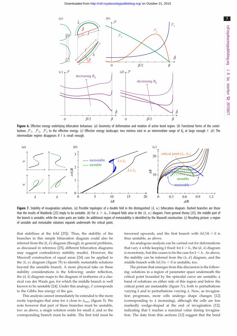
Figure 6. Effective energy underlying bifurcation behaviour. (a) Geometry of deformation and rotation of active bend region. (b) Functional forms of the contri-butions F 1, F 2, F 3 to the effective energy. (c) Effective energy landscape: two minima exist in an intermediate range of R0 at large enough ‘. (d ) Theintermediate regime disappears if ‘ is small enough.
k k 0 5 10 15 200
1
2
3
metastableunstable
kR0 0.3 0.6 0.9 1.2
10
20
unstable
metastable
critical point (l* , k*)
d/R
kR
l < l*
l > l*
(a) (b) (c)
/GR
Figure 7. Stability of invagination solutions. (a) Possible topologies of a double fold in the distinguished ðk, 5Þ bifurcation diagram. Dashed branches are thosethat the results of Maddocks [25] imply to be unstable. (b) For l . l*, S-shaped folds arise in the ðk, 5Þ diagram. From general theory [25], the middle part ofthe branch is unstable, while the outer parts are stable. An additional region of metastability is identified by the Maxwell construction. (c) Resulting picture: a regionof unstable and metastable solutions expands underneath the critical point.
rsif.royalsocietypublishing.orgJ.R.Soc.Interface
12:20150671
7
on October 21, 2015http://rsif.royalsocietypublishing.org/Downloaded from
that stabilizes at the fold [25]). Thus, the stability of the
branches in this simple bifurcation diagram could also be
inferred from the (k, d ) diagram (though, in general problems,
as discussed in reference [25], different bifurcation diagrams
may suggest contradictory stability results). However, the
Maxwell construction of equal areas [24] can be applied to
the ðk, 5Þ diagram (figure 7b) to identify metastable solutions
beyond the unstable branch. A more physical take on these
stability considerations is the following: under reflection,
the (d, k) diagram maps to the diagram of isotherms of a clas-
sical van der Waals gas, for which the middle branch is well
known to be unstable [24]. Under this analogy, E corresponds
to the Gibbs free energy of the gas.
This analysis cannot immediately be extended to the more
exotic topologies that arise for l close to lmax (figure 5). We
note however that part of these branches must be unstable,
too: as above, a single solution exists for small d, and so the
corresponding branch must be stable. The first fold must be
traversed upwards, and the first branch with @d=@k , 0 is
thus unstable, as above.
An analogous analysis can be carried out for deformations
that vary l while keeping k fixed: for k . k*, the (d, l) diagram
is monotonic, but this ceases to be the case for k , k*. As above,
the stability can be inferred from the (l, d) diagram, and the
middle branch with @d=@l , 0 is unstable, too.
The picture that emerges from this discussion is the follow-
ing: solutions in a region of parameter space underneath the
critical point bounded by the spinodal curve are unstable; a
band of solutions on either side of this region and below the
critical point are metastable (figure 7c), both to perturbations
varying k and to perturbations varying l. Now, as invagina-
tion progresses, more cells undergo shape changes [12]
(corresponding to l increasing), although the cells are less
markedly wedge-shaped at the end of invagination [12],
indicating that k reaches a maximal value during invagina-
tion. The data from thin sections [12] suggest that the bend

0 0.2 0.4 0.6 0.8 1.0
10
20
30
increasingl
max
rp/R1 0.75
rp = R
lmax = pR/2
k *R
l* / R
Figure 8. Contraction and the critical point. Trajectories of critical point inparameter space as lmax is varied, for different values of rp. Thin dottedlines are curves of constant lmax. At constant lmax, increased contractionleads to decreased k* and increased l*.
rsif.royalsocietypublishing.orgJ.R.Soc.Interface
12:20150671
8
on October 21, 2015http://rsif.royalsocietypublishing.org/Downloaded from
region does not expand into the anterior hemisphere until later
stages of inversion; this corresponds to lmax � pR=2 being
fixed during invagination. The corresponding paths in par-
ameter space may lead to very different behaviour: if
invagination is to be stable, it must move around the critical
point; if it passes through the region of in- and metastability
underneath, the shell undergoes a subcritical snapping tran-
sition between the ‘shallow’ and ‘deep’ invagination states on
either side of the metastable region. (This makes this kind of
instability different from the classical, supercritical buckling
instability of a compressed rod or a ‘popper’ toy [27], and
more akin to the snap closure of a Venus flytrap [28].) How-
ever, no such snapthrough shows up during invagination in
the dynamic data of Hohn et al. [19] (the sudden acceleration
reported there only occurs after invagination has completed).
The present mechanical analysis and these dynamic data thus
limit the parameter paths to those that eschew the unstable
region underneath the critical point, and reconciles the observed
cell shape changes to the stable dynamics: initially, a narrow
band of cells undergoes cell shape changes, thereby acquiring
a high intrinsic curvature. This region of cells then widens,
moving around the critical point, whereupon the preferred
curvature relaxes and posterior inversion can complete.
3.2.3. Contraction and criticalityFor different values of lmax, the critical point traces out a trajec-
tory in parameter space, characterized by k* and l* (figure 8).
As lmax increases, k* increases, whereas l* decreases. Thus,
the closer to the equator, the more difficult invagination is,
not only because there is less room to fit the posterior into
the anterior, but also because a stable invagination requires
narrower, and narrower invaginations of higher and higher
intrinsic curvature.
We are left to explore how contraction affects the position
of the critical point, and hence the invagination. We introduce
a reduced posterior radius rp , R as in reference [19]
(figure 4a), and modify the intrinsic curvatures and stretches
accordingly (figure 4b–d). Numerically, we observe that, at
constant lmax, increasing contraction (i.e. reducing rp) decreases
the critical curvature k*, and increases l* (figure 8). Hence, con-
traction aids invagination not only geometrically, but also
mechanically: first, it allows invagination close to the equator
(which would otherwise be prevented by different parts of
the shell touching), and second, it makes stable invagination
easier, by reducing k*. Thus, again, contraction appears as a
mechanical means to overcome global geometric constraints.
4. ConclusionIn this paper, we have explored perhaps the simplest intrinsic
deformations of a spherical shell: elastic and geometric effects
conspire to constrain deformations resulting from a localized
region of intrinsic bending. Contraction, a somewhat more
global deformation, alleviates these constraints and thereby
facilitates the stable transition from one configuration of the
shell to another. This rich mechanical behaviour makes a
mathematically interesting problem in its own right, yet this
analysis has implications for Volvox inversion and wider
material design problems.
Experimental studies of Volvox inversion [12,19] had
revealed the existence of posterior contraction, and indeed,
the simple elastic model that underlies this paper can only
reproduce in vivo shapes once posterior contraction is included
[19]. Of course, contraction is an obvious means of creating a
disparity in the anterior and posterior radii required ultimately
to fit one hemisphere into the other, but the present analysis
reveals that, beyond this geometric effect, there is another,
more mechanical side to the coin: if contraction is present,
lower intrinsic curvatures, i.e. less drastic cell shape changes,
are required to stably invert the posterior hemisphere. This
ascribes a previously unrecognized additional role to these sec-
ondary cell shape changes (i.e. those occurring away from the
main bend region): just as the shape of the deformed shell
arises from a glocal competition between elastic and geometric
effects, a combination of local and more global intrinsic proper-
ties allows inversion to proceed stably. Thus, as we have
pointed out previously, this mechanical analysis constrains
the parameter paths that agree with the dynamical obser-
vations of Hohn et al. [19] and thereby rationalizes the
timecourse of the observed cell shape changes. This lends
further support to the inference of Hohn et al. [19], that it is a
spatio-temporally well-regulated sequence of cell shape
changes that drives inversion. Thus, the remarkable process
of Volvox inversion is mechanically more subtle than it may
initially appear to be.
Intrinsic deformations that allow transitions of an elastic
object from one configuration to another are of inherent interest
in the material design context, and divide into two classes: first,
snapping transitions for fast transitions between states, studied
in reference [3], and second, stable sequences of intrinsic defor-
mations. The glocal behaviour of the latter is illustrated by the
present analysis: in particular, additional transformations
such as contraction can increase the number of stable par-
ameter paths between configurations of the elastic object. In
this material design context, non-axisymmetric deformations
such as polygonal folds or wrinkles [29] could also become
important, and may warrant a more detailed analysis.
Data accessibility. See www.damtp.cam.ac.uk/user/gold/datarequests.html.
Authors’ contributions. P.A.H. and R.E.G. contributed to the conceptionand design of the research, P.A.H. performed calculations andanalyses, P.A.H. and R.E.G. contributed to writing the manuscript.
Competing interests. We declare we have no competing interests.

rsif.royalsocietypublishing.orgJ.R.Soc.Interface
12:20150671
9
on October 21, 2015http://rsif.royalsocietypublishing.org/Downloaded from
Funding. This work was supported in part by an EPSRC studentship(P.A.H.), an EPSRC Established Career Fellowship (R.E.G.) and aWellcome Trust Senior Investigator Award (R.E.G.).
Acknowledgements. We thank Stephanie Hohn, Aurelia R. Honerkamp-Smith and Philipp Khuc Trong for extensive discussions, and ananonymous referee for insightful comments.
Appendix A. Governing equationsIn this appendix, we sketch the derivation of the Euler–
Lagrange equations of the energy functional (2.4), following
Knoche & Kierfeld [22]. The variation takes the form
dE2p¼ðpR
0
rðNsdEs þNfdEfÞdsþðpR
0
rðMsdKs
þMfdKfÞds, ðA 1Þ
where we have introduced the stresses and moments
Ns ¼ CðEs þ nEfÞ, Nf ¼ CðnEs þ EfÞ ðA 2aÞ
and
Ms ¼ DðKs þ nKfÞ, Mf ¼ DðnKs þ KfÞ, ðA 2bÞ
with C ¼ Eh=ð1� n2Þ and D ¼ Ch2=12: (These stresses and
moments are expressed here relative to the undeformed
configuration.)
The deformed shape of the shell is characterized by the radial
and vertical coordinates r(s) and z(s), as well as the angle b(s)that the normal to the deformed shell makes with the vertical
direction. These geometric quantities obey the equations [22]
drds¼ fs cosb,
dzds¼ fs sinb and
db
ds¼ fsks: ðA 3Þ
We note that one of these is redundant. The variations dEs, dEf,
dKs, dKf are purely geometrical, and one shows that [22]
dEs ¼ secbdr0 þ fs tanbdb, dEf ¼drr
ðA 4aÞ
and
dKs ¼ db0, dKf ¼cosb
rdb: ðA 4bÞ
The variation (A 1) thus becomes
dE2p¼ [[rNs secbdrþ rMs db]]�
ðpR
0
d
dsðrNs secbÞ�Nf
� �drds
þðpR
0
r fsNs tanbþMf cosb� d
dsðrMsÞ
� �dbds,
ðA 5Þ
upon integration by parts, whence
r fsNs tanbþMf cosb� d
dsðrMsÞ ¼ 0 ðA 6aÞ
and
d
dsðrNs secbÞ �Nf ¼ 0: ðA 6bÞ
These equations, together with two of the geometric relations
(A 3), describe the shape of the deformed shell. For numeri-
cal purposes, it is convenient to remove the singularity at
b ¼ p/2 by introducing the transverse shear tension [20,22],
Q ¼ �Ns tanb, expressed here relative to the undeformed con-
figuration. Force balance arguments [20,22] show that Q obeys
d
dsðrQÞ þ r fsksNs þ r ffkfNf ¼ 0: ðA 7Þ
The solution Q ¼ �Ns tanb is selected by the boundary
condition Q(0) ¼ 0. At the poles of the shell, the equations
have singular terms in them, but these singularities are either
removable or the appropriate boundary values are set by sym-
metry arguments [22]. This allows appropriate boundary
conditions and values to be derived.
Appendix B. Asymptotic detailsIn this appendix, we discuss the details of the asymptotics
summarized in the main body of the paper.
B.1. Asymptotics of small rotationsWe start by discussing the detailed solution for pure invagi-
nation. Upon non-dimensionalizing distances with R and
stresses with Eh, the Euler–Lagrange equations of (2.4),
derived in appendix A, can be cast into the form
fsS sin u tanb� 12 cosbð1� nb0 � sinb cosecuÞ
� 12 d
duðb0 sin uþ nðsinb� sin uÞÞ ¼ k0ðuÞ
ðB 1aÞ
and
d
duðS secb sin uÞ � A� nS ¼ 0, ðB 1bÞ
with the small parameter
12 ¼ 1
12ð1� n2Þh2
R2� 1: ðB 2Þ
In these equations, S is the non-dimensional meridional
stress, and A ¼ ef is the dimensionless hoop strain. The con-
tribution from the intrinsic curvature is
k0ðuÞ ¼ 12 nk0s ðuÞ cosb� d
duðk0
s sin u� �
: ðB 3Þ
The equations are closed by the geometric relation
d
duðA sin uÞ ¼ fs cosb� cos u: ðB 4Þ
Introducing g ¼ ðd=dÞ1=2, scaling gives the leading
balances S � 12g=d2, S=d � A and A=d � g in (B 1, B 4).
Hence, d � 11=2, and we define an inner coordinate j via
u ¼ Qþ dj: We also introduce the expansions
b ¼ Qþ gðb0 þ gb1 þ g2b2 þ � � �Þ, ðB 5aÞA ¼ dgða0 þ ga1 þ � � �Þ and ðB 5bÞS ¼ d2g cotQðs0 þ gs1 þ � � �Þ: ðB 5cÞ
This further proves the scaling fs ¼ 1þOðdgÞ that we have
assumed in (3.1).
The pure invagination configuration is forced by intrinsic
curvature that differs from the curvature of the undeformed
sphere in a region of width l about u ¼ Q, where k0s ¼ �k:
Writing L ¼ l=11=2, we thus have, at leading order,
k0sðjÞ ¼ �
d1=2
13=4K Hðjþ 1
2LÞ �Hðj� 12LÞ
, ðB 6Þ
where k ¼ d1=21�3=4K, and where H denotes the Heaviside
function. Thus
k0ðjÞ ¼ 13=4d1=2K0ðjÞ sinQ, ðB 7Þ
where K0ðjÞ ¼ K½dðjþ 12LÞ � dðj� 1
2L�: We note that
g3 � gd provided that d� 1 (which we shall assume to be

rsif.royalsocietypublishing.orgJ.R.Soc.Interface
12:20150671
10
on October 21, 2015http://rsif.royalsocietypublishing.org/Downloaded from
the case); thus, we may set u ¼ Q to the order at which we are
working. Expanding (B 1, B 4), we then find
s0 � b000 ¼ K0ðjÞ, s00 � a0 ¼ 0, a00 ¼ �b0, ðB 8Þ
at lowest order, where dashes now denote differentiation
with respect to j. At next order,
s1 þ s0b0 secQ cosecQ� b001 ¼ 0 ðB 9aÞ
and
s01 þd
djðb0s0Þ sinQ secQ� a1 ¼ 0, ðB 9bÞ
with a01 ¼ �b1 � 12b
20 cotQ: We are left to determine the match-
ing conditions by expanding (3.1) to find
u0r ¼ �dgb0 sinQ� dg2ðb1 sinQþ 12b
20 cosQÞ
� dg3ðb2 sinQþ b0b1 cosQ� 16b
30 sinQÞ
ðB 10aÞ
and
u0z ¼ dgb0 cosQþ dg2ðb1 cosQ� 12b
20 sinQÞ
þ dg3ðb2 cosQ� b0b1 sinQ� 16b
30 cosQÞ,
ðB 10bÞ
up to corrections of order Oðdg4, d2gÞ: Applying (3.2b), at
lowest order, we find ð1
�1
b0dj ¼ 0: ðB 11Þ
At next order, (3.2b) is a system of two linear equations for
two integrals, with solutionð1
�1
b20dj ¼ 2 sinQ and
ð1
�1
b1dj ¼ � cosQ: ðB 12Þ
In particular, the resulting condition on the leading-order
solution has only arisen in the second-order expansion of the
matching conditions. Similarly, at order Oðdg3Þ, we findð1
�1
b0b1dj ¼ 0: ðB 13Þ
The leading-order problem is thus
b00000 þ b0 ¼ Kðd00ðjþ 12LÞ � d00ðj� 1
2LÞÞ, ðB 14Þ
with matching conditions (B 11) and the first of (B 12). Sym-
metry ensures that the first of (B 11) is satisfied. After a
considerable amount of algebra, the first of (B 12) reduces
to a relation between K and L,
K2 ¼ 8ffiffiffi2p
sinQ
1þ e�L=ffiffi2pðffiffiffi2p
L� 1Þ sinðL=ffiffiffi2pÞ � cosðL=
ffiffiffi2pÞ
� � :ðB 15Þ
Symmetry also implies that there is no inward rotation of
the midpoint of the invagination at this order. Rather, inward
folding is a second-order effect, for which we need to
consider the second-order problem,
b00001 þ b1 ¼d2
dj2ðb0s0Þ � 1
2b20
( )cotQ, ðB 16Þ
with matching conditions (B 13) and the second of (B 12). The
rotation of the midpoint of the invagination is thus
DbðiÞ ¼ ðBðiÞðLÞ cosQÞ d11=2
, ðB 17Þ
where B(i)(L) is determined by the solution of (B 16). The
detailed solution reveals that
BðiÞðLÞ ¼2ffiffiffi2p
e�L=2ffiffi2p
4eL=2ffiffi2p
sinðL=ffiffiffi2pÞ � eL=
ffiffi2p
sinðL=2ffiffiffi2pÞ � 3 sinð3L=2
ffiffiffi2pÞ þ ðeL=
ffiffi2p� 1Þ cosðL=2
ffiffiffi2pÞ
h i5 eL=
ffiffi2pþ ð
ffiffiffi2p
L� 1Þ sinðL=ffiffiffi2pÞ � cosðL=
ffiffiffi2pÞ
h i , ðB 18Þ
The calculation for contraction is similar, but lacks the
complication of terms jumping order as above. It is worth
noting, however, that the solutions for pure invagination
and contraction have the same symmetry at order Oðg2Þ,and so, in particular, (B 13) is satisfied for both solutions.
Hence, the solutions for pure invagination and contraction
can indeed be superposed at this order, as claimed in the
main text.
B.2. Asymptotics of large rotationsIn the above analysis, we restricted ourselves to small
deviations of the normal angle from the spherical configura-
tion, so that the problem remained analytically tractable.
While the leading scaling balances remain the same for large
rotations, the resulting nonlinear ‘deep-shell equations’
cannot be rescaled, so that the dependence on Q drops
out [21]. Some further insight can, however, be gained in
the shallow-shell limit Q�1: in terms of the inner coordinate
j, we write
bðjÞ ¼ QBðjÞ and SðjÞ ¼ 1SðjÞ: ðB 19Þ
In the absence of forcing by intrinsic curvatures or stretches,
the leading-order balance is
2S00 ¼ 1� B2 and B00 ¼ SB, ðB 20Þ
where dashes denote, as before, differentiation with respect to j.
This balance also arises in the study of a spherical shell
pushed by a plane [21]: at large enough indentations, the
shell dimples and the plane remains in contact with it only
in a circular transition region joining up the undeformed
shell to the isometric dimple. With the matching conditions
B!+1 as j!+1, (B 20) describe the leading-order
shape of this transition region [21]. Remarkably, this defor-
mation is independent of the contact force, which only
arises at the next order in the expansion [21].
The appropriate boundary conditions for the invagina-
tion case are B! 1 as j!+1, and non-constant solutions
of (B 20) can indeed be found numerically (some solutions
are shown in figure 9). In these modes, the deformations are,
in a sense, large compared with the moments resulting from
the intrinsic curvature imposed, making them geometrically
‘preferred’. Their existence lies at the heart of the bifurcation
behaviour discussed in the main text.

xB
S
1B
S
1
x xB
S
1
Figure 9. Examples of ‘preferred’ deformation modes, which are solutions of(B 20). Of the modes shown, the middle one has the lowest elastic energy.
2cc
DJ
b
b
bb
ˆ
(a) (b)
Figure 10. Geometric details in the derivation of the effective energy. (a)Hoop strains generated by rotation and inward bending. (b) Geometry of for-mation of second bend region: close-up of the region where the active bendregion matches up to the undeformed shell.
rsif.royalsocietypublishing.orgJ.R.Soc.Interface
12:20150671
11
on October 21, 2015http://rsif.royalsocietypublishing.org/Downloaded from
Appendix C. Geometric detailsIn this appendix, we discuss the details of the geometrical
approximations that lead to the effective energy discussed
in the main body of the paper.
We restrict to the case ‘� R, in which limit we may
approximate ‘ ¼ l: It is most convenient to express the geo-
metric quantities in terms of the angle 2x ¼ l=R intercepted
by the deformed bend region (figure 10a). By definition,
‘
l¼ sinx
x, ðC 1Þ
and so the leading-order strain balances (3.6), which match the
undeformed regions on either side of the active bend region to
that region, reduce to
cos b ¼ x
sinxcosb, ðC 2Þ
in this approximation, and the deformed configuration is
described in terms of the single parameter x (or, equivalently
and implicitly, b ).
We now turn to the three physical effects mentioned
in the main paper. The curvature in the bend region is
1=R ¼ 2x=‘ in our approximation, and so the contribution
from the preferred curvature of the bend region takes
the form
F 1
Eh/ h2ð‘R sinbÞ 2x
‘� 1
R0
� �2
, ðC 3Þ
where the first factor in parentheses corresponds to the
area of the undeformed bend region, and where we have
discarded numerical prefactors.
The next contribution to the effective energy is somewhat
more subtle: as the active region bends inwards, its midpoint
moves inwards by a distance D (figure 10a). Geometry
implies that
D ¼ Rð1� cos xÞ sin b ¼ ‘ 1� cos x
2xsin b : ðC 4Þ
The resulting extra hoop strain D=R sinb constitutes the
second contribution to the effective energy
F 2
Eh/ ð‘R sinbÞ ‘
R1� cos x
x
sin b
sinb
!2
, ðC 5Þ
where, as before, we have neglected numerical prefactors.
The final contribution arises from the second bend region
that forms as the active region bends inwards, because the
tangents to the rotated active region and the undeformed
shell do not match up any longer (figure 10b). The difference
in tangent angles is
q ¼ p� ðb� b þ xÞ: ðC 6Þ
The size of the resulting bend region is set by the bending
lengthscale d �ffiffiffiffiffiffihRp
of the shell, and is thus, in particular,
independent of ‘. Determining the precise form of the result-
ing contribution to the energy would require solving the
detailed equations describing this bend region. Here, we
postulate a simple quadratic form
F 3
Eh/
d3
Rðb � x� bÞ2, ðC 7Þ
where the scale of the prefactor is motivated by the energetics
of a Pogorelov dimple [21]. A different power law for the final
factor above would not change results qualitatively.
References
1. Helfrich W. 1973 Elastic properties of lipid bilayers:theory and possible experiments. Z. Naturforsch.28c, 693 – 703.
2. Silverberg JL, Na J-H, Evans AA, Liu B, Hull TC,Santangelo CD, Lang RJ, Hayward RC, Cohen I. 2015Origami structures with a critical transition tobistability arising from hidden degrees of freedom.Nat. Mater. 14, 389 – 393. (doi:10.1038/nmat4232)
3. Bende NP, Evans AA, Innes-Gold S, Marin LA, CohenI, Hayward RC, Santangelo CD. 2014 Geometricallycontrolled snapping transitions in shells with curvedcreases. (http://arxiv.org/abs/1410.7038)
4. Kirk DL. 1998 Volvox: molecular-genetic origins ofmulticellularity and cellular differentiation.Cambridge, UK: Cambridge University Press.
5. Weismann A. 1892 Essays on heredity and kindredbiological problems. Oxford, UK: Clarendon Press.
6. Goldstein RE. 2015 Green algae as model organismsfor biological fluid dynamics. Annu. Rev. FluidMech. 47, 343 – 375. (doi:10.1146/annurev-fluid-010313-141426)
7. Green KJ, Kirk DL. 1981 Cleavage patterns, celllineages, and development of a cytoplasmic bridgesystem in Volvox embryos. J. Cell Biol. 91, 743 – 755.(doi:10.1083/jcb.91.3.743)
8. Green KJ, Viamontes GL, Kirk DL. 1981 Mechanismof formation, ultrastructure, and function of thecytoplasmic bridge system during morphogenesis inVolvox. J. Cell Biol. 91, 756 – 769. (doi:10.1083/jcb.91.3.756)
9. Viamontes GL, Kirk DL. 1977 Cell shape changesand the mechanism of inversion in Volvox. J. CellBiol. 75, 719 – 730. (doi:10.1083/jcb.75.3.719)
10. Kirk DL, Nishii I. 2001 Volvox carteri as a model forstudying the genetic and cytological control ofmorphogenesis. Dev. Growth Differ. 43, 621 – 631.(doi:10.1046/j.1440-169X.2001.00612.x)
11. Hallmann A. 2006 Morphogenesis in the familyVolvocaceae: different tactics for turning an embryoright-side out. Protist 157, 445 – 461. (doi:10.1016/j.protis.2006.05.010)
12. Hohn S, Hallmann A. 2011 There is more than oneway to turn a spherical cellular monolayer insideout: type B embryo inversion in Volvox globator.BMC Biol. 9, 89. (doi:10.1186/1741-7007-9-89)

rsif.royalsocietypublishing.orgJ.R.Soc.Interface
12:2015
12
on October 21, 2015http://rsif.royalsocietypublishing.org/Downloaded from
13. He B, Doubrovinski K, Polyakov O, Wieschaus E.2014 Apical constriction drives tissue-scalehydrodynamic flow to mediate cell elongation.Nature (Lond.) 508, 392 – 396. (doi:10.1038/nature13070)
14. Lowery LA, Sive H. 2004 Strategies of vertebrateneurulation and a re-evaluation of teleost neuraltube formation. Mech. Dev. 121, 1189 – 1197.(doi:10.1016/j.mod.2004.04.022)
15. Eiraku M, Takata N, Ishibashi H, Kawada M,Sakakura E, Okuda S, Sekiguchi K, Adachi T, Sasai Y.2011 Self-organizing optic-cup morphogenesis inthree-dimensional culture. Nature (Lond.) 472, 51 –56. (doi:10.1038/nature09941)
16. Sawyer JM, Harrell JR, Shemer G, Sullivan-Brown J,Roh-Johnson M, Goldstein B. 2010 Apicalconstriction: a cell shape change that can drivemorphogenesis. Dev. Biol. 341, 5 – 19. (doi:10.1016/j.ydbio.2009.09.009)
17. Odell GM, Oster G, Burnside A. 1981 The mechanicalbasis of morphogenesis. Dev. Biol. 85, 446 – 462.(doi:10.1016/0012-1606(81)90276-1)
18. Howard J, Grill SW, Bois JS. 2011 Turing’s nextsteps: the mechanochemical basis ofmorphogenesis. Nat. Rev. Mol. Cell Bio. 12,392 – 398. (doi:10.1038/nrm3120)
19. Hohn S, Honerkamp-Smith A, Haas PA, Khuc TrongP, Goldstein RE. 2015 Dynamics of a Volvox embryoturning itself inside out. Phys. Rev. Lett. 114,178101. (doi:10.1103/PhysRevLett.114.178101)
20. Libai A, Simmonds JG. 2006 The nonlinear theory ofelastic shells. Cambridge, UK: Cambridge UniversityPress.
21. Audoly B, Pomeau Y. 2010 Elasticity and geometry.Oxford, UK: Oxford University Press.
22. Knoche S, Kierfeld J. 2011 Buckling of sphericalcapsules. Phys. Rev. E 84, 046608. (doi:10.1103/PhysRevE.84.046608)
23. Timoshenko S, Goodier JN. 1951 Theory of elasticity.New York, NY: McGraw Hill.
24. Landau LD, Lifshitz EM. 1980 Statistical physics.Oxford, UK: Butterworth-Heinemann.
25. Maddocks JH. 1987 Stability and folds. Arch. Ration.Mech. Anal. 99, 301 – 328. (doi:10.1007/BF00282049)
26. Knoche S, Kierfeld J. 2014 Osmotic buckling ofspherical capsules. Soft Matter 10, 8358 – 8369.(doi:10.1039/C4SM01205D)
27. Pandey A, Moulton DE, Vella D, Holmes DP. 2014Dynamics of snapping beams and jumping poppers.Europhys. Lett. 105, 24001. (doi:10.1209/0295-5075/105/24001)
28. Forterre Y, Skotheim JM, Dumais J, Mahadevan L.2005 How the Venus flytrap snaps. Nature (Lond.)433, 421 – 425. (doi:10.1038/nature03185)
29. Vella D, Ajdari A, Vaziei A, Boudaoud A. 2011Wrinkling of pressurized elastic shells. Phys. Rev. Lett.107, 174301. (doi:10.1103/PhysRevLett.107.174301)
0
67 1