Elastic Waves in Timoshenko Beams: The 'Lost and Found' of an Eigenmode

Elastic Waves in Timoshenko Beams: The 'Lost and Found' of an EigenmodeAuthor(s): Atul BhaskarSource: Proceedings: Mathematical, Physical and Engineering Sciences, Vol. 465, No. 2101 (Jan.8, 2009), pp. 239-255Published by: The Royal SocietyStable URL: http://www.jstor.org/stable/30245439 .

Accessed: 14/06/2014 21:16

Your use of the JSTOR archive indicates your acceptance of the Terms & Conditions of Use, available at .http://www.jstor.org/page/info/about/policies/terms.jsp

.JSTOR is a not-for-profit service that helps scholars, researchers, and students discover, use, and build upon a wide range ofcontent in a trusted digital archive. We use information technology and tools to increase productivity and facilitate new formsof scholarship. For more information about JSTOR, please contact [email protected].

.

The Royal Society is collaborating with JSTOR to digitize, preserve and extend access to Proceedings:Mathematical, Physical and Engineering Sciences.

http://www.jstor.org

This content downloaded from 62.122.73.250 on Sat, 14 Jun 2014 21:16:32 PMAll use subject to JSTOR Terms and Conditions

http://www.jstor.org/action/showPublisher?publisherCode=rsl

http://www.jstor.org/stable/30245439?origin=JSTOR-pdf

http://www.jstor.org/page/info/about/policies/terms.jsp


PROCEEDINGS OF-

THE ROYAL SOCIETY SOCIETY

Proc. R. Soc. A (2009) 465, 239-255 doi:10.1098/rspa.2008.0276

Published online 8 October 2008

Elastic waves in Timoshenko beams: the 'lost and found' of an eigenmode

BY ATUL BHASKAR*

Aeronautics & Astronautics, School of Engineering Sciences, University of Southampton, Southampton S017 1BJ, UK

This paper considers propagating waves in elastic bars in the spirit of asymptotic analysis and shows that the inclusion of shear deformation amounts to singular perturbation in the Euler-Bernoulli (EB) field equation. We show that Timoshenko, in his classic work of 1921, incorrectly treated the problem as one of regular perturbation and missed out one physically meaningful 'branch' of the dispersion curve (spectrum), which is mainly shear-wise polarized. Singular perturbation leads to: (i) Timoshenko's solution 0(1)

~ 0(c2k*2)] and (ii) a singular solution 0*2) ~ (1/2(2) + O(k*)2; e, w* and k* are the non-dimensional slenderness, frequency and wavenumber, respectively. Asymptotic formulae for dispersion, standing waves and the density of modes are given in terms of f. The second spectrum-in the light of the debate on its existence, or not-is discussed. A previously proposed Lagrangian is shown to be inadmissible in the context. We point out that Lagrangian densities that lead to the same equation(s) of motion may not be equivalent for field problems: careful consideration to the kinetic boundary conditions is important. A Hamiltonian formulation is presented-the conclusions regarding the validity (or not) of Lagrangian densities are confirmed via the constants of motion.

Keywords: flexural elastic waves; singular perturbation; Lagrangian mechanics; Hamiltonian; Timoshenko beam

1. Introduction and field equations

Elastic waves in thin structures play a central role in many problems in engineering and physics as diverse as those involving geodynamics, piezo- electricity, ultrasonics of crystals, nanomechanics, aeronautics and a host of other structural dynamics problems. Of the various wave types, flexural or bending waves associated with the motion of material points transverse to the propagation direction is of great importance because thin structures are relatively soft in flexure than in axial deformation. In particular, wave motion in beams, plates and shells is of great interest in the area of elastodynamics. The impact of Stephen Timoshenko's work in the area is undisputed (over a thousand citations in the last 25 years). His seminal paper (Timoshenko 1921) effected a major advancement to the theory following the works of Euler, Bernoulli and Rayleigh. Euler and Bernoulli (EB) assumed that cross sections normal to the

*[email protected]

Received 6 July 2008 Accepted 5 September 2008 239 This journal is a 2008 The Royal Society



240 A. Bhaskar

axis of an elastic beam remain plane and normal during motion. This amounts to neglecting shear deformation (e.g. Landau & Lifshitz 1989). This model becomes increasingly inaccurate and predicts an infinite wave speed for an infinitesimal wavelength. Rayleigh (1877) refined the EB model by including the kinetic energy due to the rotation of the cross section. This achieves a finite wave speed; however, the predictions are quantitatively inaccurate for progressively short waves.

Timoshenko recognized the deficiency of the EB model and introduced a correction in his 1921 paper, now regarded a classic in the field. The genius of his work lies in identifying shear of the cross section with respect to the axis as the most important degree of freedom missing in the EB model while still allowing that cross sections remain approximately plane during motion. Inclusion of shear increases the range of applicability of one-dimensional models substantially. Interestingly, Timoshenko incorrectly treated the problem as one of regular perturbation (surprisingly unnoticed so far), but was fortunate in retaining a family of roots that results in the improvement of the EB theory. He was unlikely to be aware of any formal notions of singular perturbation because the subject was still in its infancy. Prandtl's boundary-layer solution in fluid mechanics (Prandtl 1904; more formally Blasius 1908) is perhaps the first known case of singular perturbation. The WKBJ method (Jeffreys 1924; Brillouin 1926; Kramers 1926; Wentzel 1926) appeared in 1924-1926. Formal developments in the singular perturbation theory came much later.

Since Timoshenko's original motivation was to improve the theory of Euler- Bernoulli-Rayleigh, the family of roots discussed in the 1921 paper has been studied in great details. By contrast, a second set of roots that appears as a consequence of the modified deformation kinematics has received relatively little attention. Levinson & Cook (1982), Stephen (1982, 2006), Chervyakov & Nesterenko (1993), Nesterenko (1993), Chan et al. (2002) and Stephen & Puchegger (2006) should be credited for studies on the second set of roots (sometimes known as the 'second spectrum'). Trabucho & Viano (1990) used asymptotic analysis in the context of Timoshenko beams but for a different purpose: to determine the shear coefficient. Indeed, Huang (1961) provided the complete solution of the frequency equation and the normal modes for standing waves in beams of finite extent under various support conditions (a minor typographical error was recently corrected by Smith (2008)). However, the debate on the existence and the validity of the second set of roots has continued. Smith (2008) found that their finite-element calculations for a thin cylinder do not match with those predicted by the Timoshenko theory. Since Smith (2008) used a thin cylinder as a 'beam', it may be that the discrepancy is due to the shell modes contributing to the response and thus theirs is perhaps a case of unfair comparison.

The Timoshenko model assumes a displacement field in the x-, y- and z-directions as (Dym & Shames 1972)

u1(x, y, z, t) = --Zvi(x, t), 2 = 0, U3 = W(X, t), (1.1)

where w is the transverse displacement; 4, = w,x(x,

t) - 0(x, t) is the rotation of the cross section due to bending only, where 0 is the shear angle of the cross section and subscript after a comma denotes differentiation; x is the propagation direction; z is the transverse direction; y is the direction perpendicular to the

Proc. R. Soc. A (2009)



Elastic waves in Timoshenko beams 241

plane of the motion; and t is time. Now, aE= - z/,, and Ez= 1/2(w,x- V) are the

only non-zero components of the strain tensor. The Lagrangian L= T- U= (1/2)S d V-(1/2) J dV is a volume integral simplified as

L =p +pAEl,+KGA(w,x )2 dx. (1.2) Here, T is the kinetic energy; U is the strain energy; p is the density; E is Young's modulus; I is the second moment of the cross-sectional area; G is the shear modulus; A is the cross-sectional area; K is the Timoshenko shear coefficient; and a dot indicates d/dt. Applying Hamilton's principle, 6 ft L dt= 0 (5 means the variation of), a pair of coupled field equations in the variables w and i/,

pAib -KGA(w,z - P,z) = 0 plI - EIV,x - K GA(w,l - l) = 0 (1.3)

is obtained. The boundary conditions (BC) are given by

w, -4=O0 or 6w=0 and 41,=O0 or 6I=0. (1.4)

Either w or '/ can be eliminated from (1.3) to get a fourth-order field equation in space and time,

p( E K) +=P0 (. EIw, + pAw,tt - pl 1 + E

W tt p

Wtttt =- (1.5)

Although (1.5) 'follows' from equations (1.3), it is not a complete description of the motion resulting from (1.1) and (1.2). The BC involving V' and 4,, cannot be expressed, for example, in terms of w and its gradients. However, both (1.3) and (1.5) lead to the same dispersion relation-both correctly produce the two branches of the dispersion curves.

In this paper, we trace the origin of the second spectrum and show how this 'branch' of the solution, which is singularly perturbed, is lost due to an incorrect use of the asymptotic analysis. In the literature, this branch is often suggested to be associated with the so-called 'ghost field' of a higher order Lagrangian (e.g. Nesterenko 1993). Correct asymptotic analysis is presented here to obtain dispersion relations, propagation modes and the density of standing waves. It is shown that the second spectrum is singularly perturbed; hence, it has no resemblance with the EB spectrum. The first spectrum is regularly perturbed and differs from the EB spectrum by a term of the order of the square of wavenumber times the radius of gyration. The doubts raised about the physical meaningfulness of the second spectrum in the literature are critically examined. We also show that the Lagrangian proposed by Nesterenko (1993) and Chervyakov & Nesterenko (1993) is not admissible; hence, clarifying why some conclusions based on this Lagrangian are questionable. A Hamiltonian description of the Timoshenko continuum is presented, and it is shown that the constant of motion is incompatible with the 'Ostrogradski Hamiltonian' presented elsewhere-the latter being associated with the Lagrangian of Chervyakov & Nesterenko (1993) and Nesterenko (1993). A Lagrangian density, contrived to produce the EB field equation but unacceptable for the context of EB mechanics, is presented-thus illustrating an important point about the variationally derived BC.




242 A. Bhaskar

2. Asymptotic analysis of the dispersion relation and the propagation modes

Equation (1.3) can be non-dimensionalized as

EW,x*x* = Wx* --

1 + E2 = ( (2.1) and the two BC (1.4) at each end of the x*-domain become

0 or 6w* =0 and =0 or 64=0. (2.2)

Here, w*=w/r, z*=z/1, t*=t/T, e= r/, =E/IKG, etc. where r= VI/A is the radius of gyration of the cross section;

T-= pl4/Er2 is the characteristic time;

and 1 is a characteristic length in the x-direction (arbitrary; can be taken as the natural length for finite-sized bars). An asterisk in the superscript denotes the corresponding non-dimensional quantity (4 does not need non- dimensionalization). Eliminating V from (2.1), a fourth-order field equation in space and time (the non-dimensional version of equation (1.5)) is obtained as

W, +W,**t'* -E2(1 a+ a) = -O. (2.3)

The EB equation corresponds to = =a=0, which is true when the characteristic length in the propagation direction is infinitely greater than the cross-sectional dimensions and that shear stiffness is much greater than elongational stiffness, i.e. KG>> E. Equation (2.1) or (2.3) is singularly perturbed over the parameter ( because the small term is associated with the highest temporal derivative in the field equations. Seeking a travelling-wave solution [w*, 4](x*, t*) = [W, if] exp{i(k*x* -w*t*)} of equation (2.1) and demanding that the determinant of the coefficient matrix must vanish, we obtain the dispersion relation D(k*, w*) as

A2a 2 + a2 = (2.4)

where y= e2; A = ((0*)2; and a= (k*)2. Owing to the non-dimensionalization, k* = kl and k* = rk. Therefore, k* <<1 means that the wavelength is much longer than the radius of gyration of the cross section.

Inclusion of shear deformation and rotary inertia was a major step forward in the one-dimensional theory. However, the procedure of ignoring the highest order term from (2.3) or (2.4) as employed by Timoshenko (and others; e.g. Dym & Shames 1972, aa7.7 and 7.12), amounts to seeking a regular expansion

S-= ao +

A1 +

A-t22 -+ --. This is inadmissible because the term O(E4), associated

with the highest order term A2, singularly perturbs the algebraic equation (2.4). Therefore, we must include singular terms such as A = _- + - - -..., n> 0 in the expansion for A (see Nayfeh 1993 or Bender & Orszag 1999). To remove the singularity, we must equate the dominant terms. This leads to n= 2 in the present case; hence, A=A-2 -2 +.-. is appropriate. Alternatively, A=2A' /2 transforms the singularly perturbed problem (2.4) to a regularly perturbed one in the new variable A' as

a2 - - + + a22 = 0. (2.5)

Retaining terms up to O(g) = O(E2) in the regular expansion of A', we obtain the following asymptotic expansion for the two roots of 2 (subscripts inside





parentheses indicate the two roots):

2(1) = - a(1 + ) +"...

and (2.6)

1 a2(1 +

Since a= k*2 and p= the asymptotic dispersion relation is given by

and (2.7)

S1 [ 2k*2(l+) E4k*4

for Ek*<<1. The first root W*1) corresponds to the frequency identified by Timoshenko and it improves the parabolic EB dispersion relation WEB = k*2. For many practical materials and cross-sectional shapes, a= 4. The shear correction is then given by OTimoshenko= EB[1 - (5/2)E2k*2 + O(e2k*4)].

The second root is a result of singular perturbation and shows a cut-on1 at 0* = 1/(E2V1) 1/(262). In physical units, wcut,,on

= Kc2/r, where c2 is the distortional wave speed VG/p. The next dominant term is With the choice of K = 72/12, the cut-on frequency is exactly equal to the cut-on frequency of the second antisymmetric mode of the Rayleigh-Lamb frequency equation (Graf 1975). Below the cut-on, the wave is evanescent and does not propagate.

The two dispersion curves associated with equation (2.1) are presented in figure la,b. The lower branch (labelled 'Timoshenko: first spectrum') is an improvement on the EB theory (the parabola labelled 'EB'). The second branch with a cut-on frequency corresponds to the second spectrum of Timoshenko equations (labelled) and must be associated with the thickness-shear mode for long waves (see the discussion following equations (2.10) and (2.11)). A one- dimensional thickness-shear theory is easy to develop by setting w= 0 in equation (1.1). The Lagrangian then becomes

LTS = ~ {PII2} - {EII , dx, (2.8)

where the subscript TS means thickness shear. The process of taking the variation leads to the field equation

pl - + KGA/1 = 0. (2.9) The corresponding dispersion curve corresponding to this one-dimensional theory is obtained as the hyperbola (4 - E2ak*2 = 1 (labelled 'one-dimensional TS'). The second spectrum and the one-dimensional TS branches are very close (figure 1 a); the difference is due to the extra flexural degree of freedom granted to the Timoshenko model. The long-wave asymptotes are labelled LWA1 and LWA2 for the first and the second spectra. Note that they diverge with increasing Ek*.

1Some authors use the term 'cut-off', instead.




244 A. Bhaskar

(a) 120 Timoshenko: second spectrum

100 -

LWA2

80 /

dimensional , 60 TS , -1 -1/2k*

Euler-Bernoulli E 40 Timoshenko:

20

,,

LWA l SLWA1 first spectrum

0 0.1 0.2 0.3 0.4 0.5 0.6 0.7 0.8 0.9 1.0

slenderness x non-dimensional wavenumber (Ek*)

(b) 120

100-

Co

80-

thickness shear 60

a 40 0

Timoshenko Euler-Bernoulli P 20 complex branches

0 0.1 0.2 0.3 0.4 0.5 0.6 0.7 0.8 0.9 1.0

slenderness x Im(non-dimensional wavenumber) (Ek*)

Figure 1. Dispersion curves and their asymptotes. (a) Propagating waves on the real wavenumber versus real frequency plane. (b) Evanescent waves on the imaginary wavenumber versus real frequency plane.

The EB model affords only one degree of freedom (transverse displacement) per cross section. The Timoshenko model, by contrast, is described by two coupled partial differential equations (PDEs); hence, there are two valid branches of the dispersion curve. The extra degree of freedom reduces the frequency (given a wavenumber) according to Rayleigh's well-known theorem (the lowest eigenvalue of a constrained system is greater than or equal to the lowest eigenvalue of the unconstrained system). Hence, the Timoshenko bending branch is lower than both





the EB and the one-dimensional thickness-shear branches (both are 'constrained' models: the constraints being 'no-shear' and 'no-flexure', respectively). When extra flexibility is introduced, each new degree of freedom provides a new branch of the dispersion relation (less accurate with respect to a three-dimensional theory than the already existing branches) and the existing branches progressively improve with each extra degree of freedom.2 The second spectrum, therefore, is a bonus due to the extra cross-sectional freedom, but it must not be expected to be as accurate as the bending branch-it is still good enough for many practical situations. Note that the relatively poor accuracy of the second spectrum with respect to detailed theories cannot be a measure of its physical meaningfulness (contrary to the suggestion of Stephen (2006) and Stephen & Puchegger (2006)).

Small changes in the equations of motion lead to small changes in the response when the solution of a differential equation is regularly perturbed. When it is singularly perturbed, the response will be significantly different (hence, not 'perturbed' in the ordinary sense of the word). The branch representing the first spectrum is regularly perturbed over the EB dispersion curve for long waves. As opposed to this, the branch corresponding to the second spectrum has no resemblance with the EB solution because it is singularly perturbed (e.g. at zero wavenumber, the EB branch and the first spectrum pass through the origin, whereas the second spectrum has a cut-on frequency). The small difference between the second spectrum and the one-dimensional thickness-shear branches is attributed to the lack of small coupling between the shear deformation and the transverse deflection, which is missing in the latter.

The evanescent waves can be obtained by setting k*--ik*. The resulting wavenumber-frequency relationship is an ellipse E4 )**2 + E2O(ik*)2 = 1 on the imaginary wavenumber-real frequency plane for the thickness-shear model (2.9)-a quarter of which is shown in figure lb and labelled 'thickness-shear'. The EB dispersion relation on this plane continues to be a parabola (ik*)4=

(o*)2. This curve is plotted in

figure lb using the label EB. The two branches of the dispersion curves of Timoshenko's equations are plotted using solid lines. Note that the agreement is quite good up to the value of liEk*l approximately equal to 0.2 (i.e. wavelength five times the radius of gyration). Interestingly, the branches of the Timoshenko equations merge and become complex (conjugate pair) for shorter evanescent waves (only the real part of the frequency is shown). The complete spectrum (i.e. a complex wavenumber for a prescribed real frequency) can be calculated by transforming a lambda-matrix problem of the form [k2A2+ kA1 + Ao(w)]u = 0 that arises out of (1.3) to a standard eigenvalue problem in a space of double the dimension (as in Bhaskar 2003)-the matrices Ao, A1 and A2 contain coefficients of the terms in equation (1.3). A complex wavenumber can result for the case of material damping (owing to a first derivative term that leads to an imaginary term in the Fourier domain), as well as for evanescent waves (spatially damped waves) even in the absence of material damping (real o can lead to complex k solutions for a lambda-matrix problem).

To understand the propagation eigenmodes, the eigenvectors of equation (1.3) are analytically obtained as

[ W, [1, i(k* 2 (2.10)

2 The 'exact' dispersion curve, of course, has an infinite number of branches when the cross section is treated as a continuum.




246 A. Bhaskar

where a(1,2) are given by (2.7). The imaginary amplitude ratio means that w and l are out of phase by 7r/2. The asymptotic expansions of the propagation modes for long waves

W(1) :

(1) = 1 : i[(ck*) -a(k*)3

+ O(efk*5)]

and (2)(2.11) W(2) =

1:2)=1 - i + k*3]

show that the dominant behaviour of the first mode is W(1) : (1) = 1 : ifk*

(which is identical to the propagation mode of the EB model for which ' = w,,). The second dispersion branch has the dominant behaviour W(2) ( 2)=iek* : 1, which is mainly shear-wise polarized as k*-+*0. These motions of the cross section are shown at the left end of figure la. The motion associated with long-wave propagation is in agreement with the normal modes presented by Downs (1976) and Chan et al. (2002). The mode of cross-sectional motion associated with the two propagation modes for long waves (transverse deflection without shear for the first spectrum and shear without transverse deflection for the second spectrum) has been observed theoretically by Chan et al. (2002). They should also be credited for providing experimental evidence for the second spectrum within a limited range of frequency. Although a direct comparison is not easy because the results of Chan et al. (2002) are for beams of finite extent as they do not measure the dispersion relation, the normal modes M3-M6 in their fig. 4 and table 3 correspond to the standing-wave counterpart of the second spectrum.

The type of motion changes with wavenumber and shear and transverse motions get mixed. Stephen (1982) found this changing behaviour in the second spectrum strange and having a 'split personality'. Changing character of motion on the travelling-wave dispersion diagram is a norm rather than exception (see Bhaskar (2003) for this perfectly normal behaviour along dispersion curves). Indeed, the split personality description is as much valid for the first spectrum as it is for the second spectrum: both branches cease to be pure shear or pure bending branches for a non-zero wavenumber. The changing character of the propagation mode along a dispersion curve is not uncommon (although Stephen (1982) finds this unusual). The reason is that the mode shapes for the travelling- wave problem is an eigenvector of a parameter-dependent eigenproblem-the wavenumber usually playing the role of the parameter on which the eigenvalues and the eigenvectors depend. This is unlike the case of standing waves (normal modes) viewpoint where the mode shape is fixed (and hence its character) given a mode number (or a natural frequency). The more interesting case is when the character of the normal modes changes sharply with the wavenumber-it is suggested by Bhaskar (2003) that this is due to eigencurve veering on the wavenumber-frequency plane. This will be studied in its generality in a future paper. Further discussion is beyond the scope of the present paper.

For infinitesimally short waves, *1) - a-1/2k*,so we have W(i) : W(1) = 1 : 0, which represents transverse motion without cross-sectional rotation. The second branch becomes w2) -1 k*, for large k*, which implies W(2) : (2) = 1 : -3iek* which is transverse motion of the axis and tilt of the cross section thrice (but opposite in sense) of what EB kinematics (1.1) dictates. Of course, no continuum model is valid in this limit of short waves.





(a) Standing waves and the density of modes

The accurate mode count (or the density of modes) is often more important than the accuracy of the individual modes (as in statistical energy analysis (SEA); Hodges & Woodhouse 1986) for studying the high-frequency dynamics of complex structures. Consider the frequency equation of standing waves in a beam of finite length with supported ends (Timoshenko 1921),

(nr)4 - + [ 2(1 + a) (n)2] + 4. (2.12) n n 4 2.2 Seeking expansions on the lines of equation (2.7), we have two sets of natural frequencies as

(0,(1)

= (n)2[1 -re2n22(1 + a)/2 +...] (2.13) + +

Timoshenko's solution is identical to ",4(1) and shows an improvement over EB values WEB = n,2, but the second set was lost by Timoshenko (1921) owing to incorrectly treating the problem as one of regular perturbation.

Equation (2.12) is quadratic in n2 for a specified value of ow = o*, say. If we treat o* as a continuous variable, for w0* <o, n < 0 but n > 0; for W* > o

nl,2 > 0; at the cut-on frequency O, n2-=0. Therefore, for frequency parameter

w* < oW, there is only one valid mode, as expected. The cumulative mode count N(w*) = n1 for w* < 6o and N(wo) = n1 + n2 for 0* > wo. The subscripts '<' or '>' denote values less than or greater than the cut-on frequency. After using properties of the sum and the product of the roots of a quadratic, the cumulative mode count is given by

S 1 2112 N(oE<) =o(I (+u) + + 1- (a-1) 4

S 2 + - 1)1/2}1/

(2.14)

N(Ew ) 2 + )W*2 *(4 1/21/2

Are the frequencies from the second set too high to be practically important? To examine this, the mode number at the cut-on frequency is obtained as (Int is the greatest integer function)

N, = N(wo) = Int [V(1+ a)/U/(7r)]. (2.15)

For slenderness c=1: 15, the mode count at cut-on Nc= 5.3; hence, the first mode in the wo series lies between the fifth and the sixth in the wT series- certainly, a moderate frequency range for many practical applications.

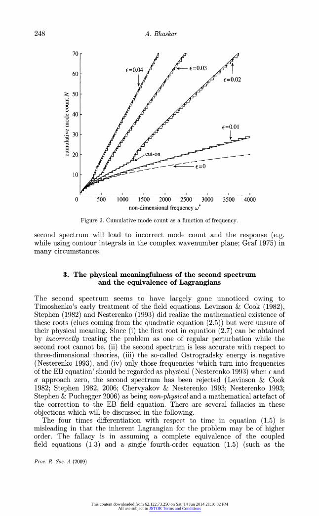
The cumulative mode count is shown in figure 2. Smooth curves depict equation (2.14); 'staircasing' refers to the numerically computed modes (a little dot appears where a mode from the second series is encountered). Both curves show a break at the cut-on frequency where the second spectrum starts contributing to the total mode count. The cut-on is at a smaller frequency for shorter beams (greater E), indicating increased importance of the second spectrum. This is particularly relevant when the excitation is in the thickness-shear mode (as in piezoelectric applications). Omitting the




248 A. Bhaskar

70

60 = 0.04 --=0.03 E0.02

4 50

S40

e=I0.01

~ 20 cut-on

10-

0 500 1000 1500 2000 2500 3000 3500 4000 non-dimensional frequency w*

Figure 2. Cumulative mode count as a function of frequency.

second spectrum will lead to incorrect mode count and the response (e.g. while using contour integrals in the complex wavenumber plane; Graf 1975) in many circumstances.

3. The physical meaningfulness of the second spectrum and the equivalence of Lagrangians

The second spectrum seems to have largely gone unnoticed owing to Timoshenko's early treatment of the field equations. Levinson & Cook (1982), Stephen (1982) and Nesterenko (1993) did realize the mathematical existence of these roots (clues coming from the quadratic equation (2.5)) but were unsure of their physical meaning. Since (i) the first root in equation (2.7) can be obtained by incorrectly treating the problem as one of regular perturbation while the second root cannot be, (ii) the second spectrum is less accurate with respect to three-dimensional theories, (iii) the so-called Ostrogradsky energy is negative (Nesterenko 1993), and (iv) only those frequencies 'which turn into frequencies of the EB equation' should be regarded as physical (Nesterenko 1993) when E and a approach zero, the second spectrum has been rejected (Levinson & Cook 1982; Stephen 1982, 2006; Chervyakov & Nesterenko 1993; Nesterenko 1993; Stephen & Puchegger 2006) as being non-physical and a mathematical artefact of the correction to the EB field equation. There are several fallacies in these objections which will be discussed in the following.

The four times differentiation with respect to time in equation (1.5) is misleading in that the inherent Lagrangian for the problem may be of higher order. The fallacy is in assuming a complete equivalence of the coupled field equations (1.3) and a single fourth-order equation (1.5) (such as the





Pais-Uhlenbeck oscillator; Nesterenko 2007). The Lagrangian density (Lagran- gian per unit length) intrinsic to the equations of Timoshenko (1.3) and (1.4) in the non-dimensional form is (subscript T refers to Timoshenko and EB refers to EB when required)

YTjT = Y .'(wi* , 1I/,t*, wI* ,I P), a*)

1 w2 + 2 -1 2 -1-4 )2] = [Wit* + ,t* - aE * (ow,-#)2. (3.1)

Although the choice of Lagrangians is not unique (e.g. Lagrangians related via, but not limited to, gauge invariance property L'= L+dF/dt describe the same circumstances of motion, dF/dt being the total time derivative of any function that depends on the generalized coordinates and time; Konopinski 1969; Lemos 1981), the need for a higher order Lagrangian seems artificial in the present context. Chervyakov & Nesterenko (1993) and Nesterenko (1993) proposed a Lagrangian density (presented here in the non-dimensional form)

= IT(W,t*,

W,t*t*, ,

[W*,t*2 -_2W,ix*x* f tt* --,)*t + 2Wt*t* Wx(3.2)

This Lagrangian does produce field equation (2.3) that is incomplete (see the remark following equation (1.5)). The BC obtained from *T are unacceptable. Since T4 leads to neither equations (1.3) nor the BC (1.4), it is inadmissible.

While constructing Lagrangians (often as a correction to another Lagrangian), it is possible in some contexts that the modified Lagrangian leads to physically unacceptable modes (known as ghost fields; e.g. Nesterenko 1989; Simon 1990). The case of the Timoshenko model in elastodynamics, however, is unambiguous: there are no ghost modes and both modes of propagation are physically meaningful. These conclusions can be easily generalized to flexural waves in plates and shells because Mindlin's equations (e.g. Dym & Shames 1972, a7.12) are generalization of Timoshenko's for the plate problem.

Equation (1.5) is sometimes regarded as the governing field equation for the Timoshenko model. Interestingly, it is often presented without any BC. The BC obtained from the 'higher order Lagrangian' are clearly incorrect and, surprisingly, remain unquestioned (e.g. by Stephen 2008). The physics of Timoshenko beams lacks four BC involving the field variable w (and its gradients) alone as demanded by (1.5). The correct BC involve a mix of w and l (and their gradients). There is no known Lagrangian that directly produces equation (1.5) together with the correct BC. Indeed, any attempt to construct a Lagrangian involving w alone is doomed to failure because t cannot be eliminated from the BC (1.4). Perhaps the only reason why the fourth-order PDE (1.5) is given any consideration is because it appears as a correction on EB equation-the latter is obtained by suppressing the last two terms. These two terms are not introduced as ad hoc correction factors while developing Timoshenko model-the basis is the kinematics of equation (1.1) followed by the application of the variational principle.

Stephen (2008) did not question the validity of the Lagrangian density (3.2). Instead, he showed that the fourth-order time differentiation in (2.3) is analogous to a coupled oscillator problem being described by a single ordinary differential




250 A. Bhaskar

equation (ODE) of the fourth order (instead of a pair of ODEs, each being a second order)-thus misplacing the focus of the issue. The fourth-order ODE can be reproduced by a Lagrangian having higher order time derivative. However, (i) we cannot assign the three initial conditions to the fourth-order ODE at will, they need to be 'borrowed' from the initial conditions associated with the pair of ODEs,3 and (ii) not only the variations are required to be co-terminus, but also their first and the second time derivatives are required to be co-terminus.4

The issue of the order of the spatial differentiation is more subtle owing to the conditions at the boundary. There are only four possible combinations of physically meaningful BC consistent with (3.1): (i) 6w*= 0 and 64a= 0 for a fixed (cantilevered) end, (ii) 6w* =0 and

/,* = 0 for a supported end, (iii) w,* - = 0

and I,* = 0 for a free end, and (iv) w,.,

-4 = 0 and 6'= 0 for a non-rotating sliding end. The fourth BC is theoretically possible but is rarely encountered in engineering practice. If there are other mechanical elements (such as a mass or a spring) that involve energy terms, then the Lagrangian must be modified accordingly. By contrast, the BC consistent with (3.2) are of dubious physical meaning.

The choice of the Lagrangian as the difference between the kinetic energy and the potential energy is common in classical mechanics but it is not limited to this. For conservative systems with finite degrees of freedom, all Lagrangians that produce the same equations of motion (ODEs) are equivalent because they predict identical causal responses. For field problems (represented by PDEs), the reproduction of the same field equations alone is not sufficient for the equivalence of Lagrangian densities. This point does not seem to have been recognized in the literature. In addition to the field equations, we require that the set of variationally consistent BC must also be identical if two Lagrangian densities were to be equivalent. To illustrate this, consider the following Lagrangian density (associated with EB beams):

SB 1 *2 0

(2. (3.3) B= I- * *

2(W,t,- W ). (3.3) EB 2( it I

Applying Hamilton's principle 6 ft1 EB dx* dt* = 0, we obtain

-t*t* + J WI + J x 2 6xw*)l ~-(wx**Iw,**

I dt* = 0. (3.4 '1 1

(3.4) 3 For example, the generalized coordinate q2 can be 'eliminated' from the pair of ODEs ql + ql - q2=0 and q2- 1 +yq2=0 to obtain

iq+ (1+y)q1+(y - 1)q, =0, but one is not free to prescribe arbitrary initial conditions q1(0) = q10, q1(0)

= v-o, 41 (0)

= a10, t4l(0) = j10 to the fourth- order ODE at will (in the way evolution equations admit arbitrarily prescribable initial state from where the future states unfold). The constraints 41(0)+a q1(0)= q2(0) and tqi(0)+ q4(0)= 42(0) on the initial conditions need to be additionally respected. 4To derive the fourth-order ODE variationally from a higher order Lagrangian, one additionally requires 641(0) = 6i1(0) = 0. Traditionally, Hamilton's principle demands co-terminus variations of the generalized coordinates ql and q2 only, i.e. 6ql = 6q2 = 0.





Since the variation 6w* is arbitrary, we obtain the governing equation of motion

W,t*t* +W,x*x*x*x* = 0, (3.5)

and the BC as either 6w*=0 (kinematic BC) or w,l*a,z,=0

(kinetic BC), and 5w, * (kinematic BC) or

w,**x,=0 (kinetic BC). The two kinetic BC can be

physically interpreted as the absence of shear force or bending moment when the ends are not restrained in transverse motion or rotation, respectively. Now consider a hypothetical Lagrangian density (note the extra two terms)

EB 2

W r * 2 WIx*

Carrying out the variations, we have

+J J (w,4*t* +w,* * dx*dt**

+J [(w,,,, +al)6w* -(w,*,-a2)6 w, *, I]dt* 0. (3.7)

This leads to the same field equation as (3.5) but the BC are now 6w*=0 (kinematic BC) or w,x,*xx a+al = 0 (kinetic BC), and 6w,*. (kinematic BC) or w,~*,X -a2 = 0 (kinetic BC). The two Lagrangian densities (3.3) and (3.6) are not equivalent because the response predicted would, in general, be different due to different kinetic BC.

One may argue that once having derived the correct field equation(s) (say, from (3.7)), one could use physically meaningful BC (not necessarily the one(s) resulting from the Lagrangian that produced the field equation(s) in the first place). This argument is unacceptable because the field equations and the BC come as a 'single package' as a result of variational process. Having taken a Lagrangian for granted, we must accept all the consequences that arise out of it and not selectively discard the ones regarding the BC. In many situations, the BC can be derived satisfactorily only by demanding variational consistency with the Lagrangian (e.g. the Kirchhoff-shear BC at the free edge of a plate).

Analogous to discrete problems, the canonical momentum density and the Hamiltonian density corresponding to aEB are given by

TEB and -EB = fEB W,* -- B (3.8) wt and similar expressions for *EB and *EB (tilde for quantities associated with

*EB). We obtain the expressions for momentum density corresponding to the Lagrangians (3.3) and (3.6) as

IrEB- =-EB -W* . The corresponding non- dimensional Hamiltonian densities are

and

* 1

(3.9)

EB = -W ( _**x) - a1w,* -a2 W,* EB 2( I Ix xl * -02WixZx Proc. R. Soc. A (2009)



252 A. Bhaskar

While there is no requirement that the Hamiltonian be identical with the total mechanical energy (the choice of the Hamiltonian as the total energy may be seen as a mere convention in mechanics), it is a conserved quantity (e.g. the total energy plus an arbitrary constant is also a conserved quantity) and, therefore, is a constant of motion. The two Hamiltonians corresponding to yEB and EB are the constants of motion given by

H B EB dx* =E* and

(3.10) HEB B d* + )dx*, EB EB dx (a1 w, *- + 2 w, x*)d*

where E* is the total (non-dimensional) mechanical energy. Carrying out integrations, we have

HEB = E* - al[w*(1, t*)- w*(0, t*)] - C2[w,* (1, t*) - W, (0, t*)]. (3.11)

Therefore, the Lagrangian density (3.6) requires the quantity HEB to be conserved. This is not only unphysical, it is also inconsistent with the conservation of HIB. We conclude again that a1B and PEB are not equivalent Lagrangian densities and that the latter is a bogus choice for describing the EB beam dynamics.

There is a further interesting implication of the above discussions to computational mechanics. Methods such as the finite-element method, Rayleigh-Ritz method, boundary-element method, etc. are often formulated variationally by expressing the Lagrangian in terms of free parameters (generalized coordinates of the discretized problem) and applying the variational principle leading to ODEs. Consider Rayleigh's method applied to a fixed-free cantilever beam subjected to a non-dimensional tip force F'(t) using, for example, a one-term displacement representation w*(x*, t*) = q(t*)x*2. Only the kinematic BC at the root of the beam (x*= 0) need to be satisfied. The Lagrangians corresponding to (3.3) and (3.6) for a beam of unit length are then

LEB= (1/2) [(q,t /3) -4q2] and LEB = LB (a1 + 2a2)q, respectively. The variation of the work done by the non-conservative forces is 6 Wc = F*6q. Applying either Hamilton's principle or Lagrange's equations, we obtain the 'discretized' equation of motion as

1 1 - q,t*t* + 4q = F* and I

q,t*t* + 4q +

(aa + 2a2) = F*, (3.12) 3 3

arising out of Y*B and -4EB, respectively. They are clearly inconsistent. This further illustrates that Y* is inadmissible in the context of the EB theory despite correctly producing the field equation (3.5). One could further construct realistic computational examples (such as in finite elements) and show that the element stiffness matrices arising out of such inadmissible Lagrangians are different from the desired ones. It is therefore reasonable to demand that, given a discretization (i.e. a discretization method and an expansion of the field variable in a chosen basis), the discretized equations arising from all equivalent Lagrangian densities must be equivalent.





Returning to the original context of Timoshenko beams, FY and aT are not equivalent Lagrangian densities because they lead to different kinetic BC-those arising out of the latter cannot be associated with the Timoshenko model. Hence, we propose that two Lagrangian densities be called equivalent if, and only if, they produce the same field equation(s) as well as the same complete set of possible BC. The Hamiltonian density corresponding to !2 is obtained by calculating the canonical momentum density fields (two of them) as

S=,=t* and r - - l = l /,t*. (3.13) -ra dw

t* O'

The Hamiltonian density for the Timoshenko deformation field is then given by

, ,1 , 1 -

i - 4((W,* __,p )2], Ye T= 7r *w* a7 -

=2 [Wit* -f (,

(.4) (3.14)

which is always positive (and equals the total energy density owing to the choice of the Lagrangian density). This is in disagreement with the Ostrogradski Hamiltonian (which is a function of w* and its spatio-temporal derivatives but independent of 4; as in Stephen (2008)) based on Nesterenko's Lagrangian. The two are incompatible-i.e. both of them cannot be constants of motion. The 'conjugate momenta' calculated by Stephen (2008; they should be momenta density for field problems, really) are also incompatible with equation (3.13). The conclusion is that Z4 is not appropriate for Timoshenko's field equations and that it has led to some unacceptable implications in the literature.

4. Conclusions

It was shown that the wave propagation problem associated with transverse motion of bars including shear deformation is singularly perturbed. It was further shown that using regular expansion for the singularly perturbed problem (as in Timoshenko's paper and elsewhere in the literature) leads to the loss of one branch of the dispersion curves (also known as the second spectrum)-often debated if it is physical or not. The first spectrum is corrected (with respect to the EB theory) by a term of the order of (2k*2, whereas the singularly perturbed branch (the second spectrum) is new and has the leading term of the order of j-2 e being the ratio of the radius of gyration and the characteristic length in the propagation direction.

It has been argued here that the single field equation, which is the fourth order in space and time, frequently used to represent Timoshenko dynamics is inappropriate in the context because: (i) it is incomplete and (ii) it lacks four physically meaningful BC.

The second spectrum is associated with thickness-shear motion (in agreement with Downs (1976) and Chan et al. (2002)) and it must not be disregarded contrary to suggestions by some authors. This propagation mode shows a cut-on frequency below which it is evanescent-the cut-on frequency being equal to the cut-on frequency of the second antisymmetric mode of the Rayleigh-Lamb frequency equation for the choice of the Timoshenko shear coefficient K= 7r2/12.




254 A. Bhaskar

An easy to develop model of thickness-shear motion having one degree of freedom per cross section shows good agreement with the second spectrum of Timoshenko equations, well up to wavelengths about five times the radius of gyration for propagating waves as well as evanescent waves.

The relatively poorer accuracy of the second spectrum (when compared with that of the first spectrum) is explained by the use of Rayleigh's theorem for systems with constraints. It was shown that the density of modes changes non- smoothly at the cut-on frequency. Ignoring the second spectrum would lead to significant inaccuracies while using methods such as the SEA.

A Hamiltonian formulation of the Timoshenko deformation field was presented, and it was shown that the Hamiltonian density (and its spatial integral: the Hamiltonian) are well-behaved positive quantities. It was shown that a previously proposed Lagrangian is inadmissible to describe the dynamics of Timoshenko beams. An example was presented to show that Lagrangians leading to the same field equation but different BC lead to intrinsically different constants of motion-hence, they are inequivalent. Finally, the Hamiltonian density of Timoshenko dynamics is found to be in disagreement with the previously proposed Ostrogradski Hamiltonian-the latter being based on an unacceptable Lagrangian. I thank several of my colleagues for their useful comments.

References

Bender, C. M. & Orszag, S. A. 1999 Advanced mathematical methods for scientists and engineers. Berlin, Germany: Springer.

Bhaskar, A. 2003 Waveguide modes in elastic rods. Proc. R. Soc. A 459, 175-194. (doi:10.1098/ rspa.2002.1013)

Blasius, P. R. H. 1908 Grenzschichten in Flussigkeiten mit kleiner Reibung. Z. Math. Phys. 56, 1-37.

Brillouin, L. 1926 La mechanique ondulatoire de Schrodinger: une methode generale de resolution par approximations successives. Comptes Rendus 183, 24-26.

Chan, K. T., Wang, X. Q., So, R. M. C. & Reid, S. R. 2002 Superposed standing waves in a Timoshenko beam. Proc. R. Soc. A 458, 83-108. (doi:10.1098/rspa.2001.0855)

Chervyakov, A. M. & Nesterenko, V. V. 1993 Is it possible to assign physical meaning to field theory with higher derivatives? Phys. Rev. D 48, 5811-5817. (doi:10.1103/PhysRevD.48.5811)

Downs, B. 1976 Transverse vibrations of a uniform, simply supported beam without transverse displacement. ASME J. Appl. Mech. 43, 671-673.

Dym, C. L. & Shames, I. H. 1972 Solid mechanics: a variational approach. New York, NY: McGraw Hill. Graf, K. F. 1975 Wave motion in elastic solids. New York, NY: Dover. Hodges, C. H. & Woodhouse, J. 1986 Theories of noise and vibration transmission in complex

structures. Rep. Prog. Phys. 49, 107-170. (doi:10.1088/0034-4885/49/2/001) Huang, T. C. 1961 The effect of rotary intertia and of shear deformation shear deformation on the

frequency and normal mode equations of uniform beams with simple end conditions. ASME J. Appl. Mech. 28, 579-584.

Jeffreys, H. 1924 On certain approximate solutions of linear differential equations of second order. Proc. Lond. Math. Soc. 23, 428-436. (doi:10.1112/plms/s2-23.1.428)

Konopinski, E. J. 1969 Classical descriptions of motion. San Fransisco, CA: W.H. Freeman and Co. Kramers, H. A. 1926 Wellenmechanik und halbzahlige Quantiseirung. Z. Phys. 39, 828-840.

(doi:10.1007/BF01451751)





Landau, L. D. & Lifshitz, E. M. 1989 Course on theoretical physics: theory of elasticity. Oxford, UK: Pergamon.

Lemos, N. A. 1981 Physical consequences of the choice of the Lagrangian. Phys. Rev. D 24, 1036-1039. (doi:10.1103/PhysRevD.24.1036)

Levinson, M. & Cook, D. W. 1982 On the two frequency spectra of Timoshenko beams. J. Sound Vib. 84, 319-326. (doi:10.1016/0022-460X(82)90480-1)

Nayfeh, A. H. 1993 Introduction to perturbation techniques. New York, NY: Wiley Classics. Nesterenko, V. V. 1989 Singular Lagrangians with higher derivatives. J. Phys. A Math. Gen. 22,

1673-1687. (doi:10.1088/0305-4470/22/10/021) Nesterenko, V. V. 1993 A theory of transverse vibration of the Timoshenko beam. PMM J. Appl.

Math. Mech. 57, 669-677. (doi:10.1016/0021-8928(93)90036-L) Nesterenko, V. V. 2007 Instability of classical dynamics in theories with higher derivatives. Phys.

Rev. D 75, 087 703. (doi:10.1103/PhysRevD.75.087703) Prandtl, L. 1904 In Verhadlungen des dritten internationalen Mathematiker-Kongress (Heidelburg),

p. 484. Rayleigh, L. 1877 The theory of sound, vol. 1, p. 186. New York, NY: Dover. (1945 Re-issue). Simon, J. Z. 1990 Higher-derivative Lagrangians, nonlocality, problems, and solutions. Phys. Rev.

D 41, 3720-3733. (doi:10.1103/PhysRevD.41.3720) Smith, R. W. M. 2008 Graphical representation of Timoshenko beam modes for clamped-clamped

boundary conditions at high frequency: beyond transverse deflection. Wave Motion 45, 785-794. (doi: 10.1016/j.wavemoti.2008.01.002)

Stephen, N. G. 1982 The second frequency spectrum of Timoshenko beams. J. Sound Vib. 80, 578-582. (doi:10.1016/0022-460X(82)90501-6)

Stephen, N. G. 2006 The second spectrum of Timoshenko beam theory: further assessment. J. Sound Vib. 292, 372-389. (doi:10.1016/j.jsv.2005.08.003)

Stephen, N. G. 2008 On the Ostrogradski instabilty for higher-order theories and the pseudo- mechanical energy. J. Sound Vib. 310, 729-739. (doi:10.1016/j.jsv.2007.04.019)

Stephen, N. G. & Puchegger, S. 2006 On the valid frequency range of Timoshenko beam theory. J. Sound Vib. 297, 1082-1087. (doi:10.1016/j.jsv.2006.04.020)

Timoshenko, S. P. 1921 On the correction of shear of the differential equation for transverse vibration of prismatic bars. Philos. Mag. 41, 744.

Trabucho, L. & Viano, J. M. 1990 A new approach of Timoshenko's beam theory by asymptotic expansion method. Math. Mod. Num. Anal. 24, 651-680.

Wentzel, G. 1926 Eine Verallgemeinerung der Quantenbedingungen fur die Zwecke der Wellenmechanik. Z. Phys. 38, 518-529. (doi:10.1007/BF01397171)




Elastic Waves in Timoshenko Beams: The 'Lost and Found' of an Eigenmode

Documents

Transcript of Elastic Waves in Timoshenko Beams: The 'Lost and Found' of an Eigenmode