Eindhoven University of Technology

MASTER

Mutual coupling between radio altimeter horn antennas on aircraft (modeled as slotantennas on a cylinder)

Verpoorte, J.

Award date:1991

DisclaimerThis document contains a student thesis (bachelor's or master's), as authored by a student at Eindhoven University of Technology. Studenttheses are made available in the TU/e repository upon obtaining the required degree. The grade received is not published on the documentas presented in the repository. The required complexity or quality of research of student theses may vary by program, and the requiredminimum study period may vary in duration.

General rightsCopyright and moral rights for the publications made accessible in the public portal are retained by the authors and/or other copyright ownersand it is a condition of accessing publications that users recognise and abide by the legal requirements associated with these rights.

• Users may download and print one copy of any publication from the public portal for the purpose of private study or research. • You may not further distribute the material or use it for any profit-making activity or commercial gain

Take down policyIf you believe that this document breaches copyright please contact us providing details, and we will remove access to the work immediatelyand investigate your claim.

Download date: 27. Jul. 2018

EINDHOVEN UNIVERSITY OF TECHNOLOGY

DEPARTMENT OF ELECfRlCAL ENGINEERING

PROFESSIONAL GROUP: Electromagnetism and Circuit Theory

Mutual coupling between radio altimeterhorn antennas on aircraft

(modeled as slot antennas on a cylinder)

by

J. Verpoorte

Report ET-6-91

This study has been performed in fulfill­ment of the requirements for the degree ofMaster of Science (ir.) at the EindhovenUniversity of Technology from August 1990until May 1991 under supervision ofdr. M.EJ. Jeuken, Eindhoven University ofTechnology and Dr.ir. P.A. Beeckman,Electromagnetics & RF Systems Group ofFokker Aircraft B.V., Schiphol-Oost.

Eindhoven, 17 mei 1991.

ABSTRACT

The aim of this study is to calculate the mutual coupling between

radio altimeter horn antennas on aircraft. The horn antennas are

modeled as radiating slots on a cylinder.

Two algorithms have been developed, according to the theory of

Borgiotti, for the calculation of mutual coupling between slots

on a ground plane. The first algorithm is a Fourier transform

method, the second an asymptotic method, valid for large

distances between the slots.

For the calculation of mutual coupling between slots on a

cylinder, two algorithms are derived, using a Green's function

(established by Boersma) for the magnetic field on a cylinder due

to a magnetic dipole. The Green's function is asymptotic for a

large radius of the cylinder. The first algorithm calculates an

asymptotic value of the mutual coupling. The second algorithm is

an approximation of the mutual coupling, valid for large

separation of the slots.

The comparison of measurements and calculations performed by

other authors with calculations produced by the algorithms

developed, shows that the algorithms for the calculations on a

cylinder are very useful for calculations on both cylinder and

ground plane.

The comparison of coupl ing calculations for slot antennas with

coupl ing measurements of radio al timeter horn antennas, shows

that the modeling of the altimeter horn antenna as a slot antenna

is to simple.

CONTENTS

1. INTRODUCTION 1

2. THE RADIO ALTIMETER SYSTEM 4

2.1 FM-CW RADAR 4

2.2 ALTIMETER ANTENNA ISOLATION 9

2.3 ALTIMETER ANTENNA MODELING 10

3. MUTUAL COUPLING BETWEEN TWO SLOTS IN A

CONDUCTING INFINITE GROUND PLANE 11

3.1 DEFINITION MUTUAL ADMITTANCE BETWEEN TWO SLOTS 11

3.2 MUTUAL ADMITTANCE FOR TWO IDENTICAL RECTANGULAR

SLOTS 15

3.3 ASYMPTOTIC EXPRESSION FOR THE MUTUAL ADMITTANCE 24

3.4 MUTUAL COUPLING BETWEEN THE SLOTS 28

4. MUTUAL COUPLING BETWEEN TWO SLOTS ON A

CONDUCTING INFINITELY LONG CIRCULAR CYLINDER 33

4.1 ASYMPTOTIC EXPRESSION FOR THE SURFACE MAGNETIC

FIELD 34

4.2 ASYMPTOTIC EXPRESSION FOR THE MUTUAL ADMITTANCE 46

4.3 APPROXIMATE ASYMPTOTIC EXPRESSION FOR THE MUTUAL

ADMITTANCE 49

4.4 MUTUAL COUPLING BETWEEN THE SLOTS ON THE CYLINDER 52

5. NUMERICAL RESULTS

5.1 DESCRIPTION OF THE PROGRAMS 53

5.1.1 Asymptotic method for the calculation of mutual

coupling between two slots on a conducting

infinite ground plane (MCA) 53

5.1.2 Fourier transform method for the calculation of

mutual coupling between two slots on a conducting

infinite ground plane (MCB) 54

5.1.3 Asymptotic method for the calculation of mutual

coupling between two slots on a conducting

infinitely long cylinder (MCC) 56

5.1.4 Approximate asymptotic method for the calculation

mutual coupling between two slots on a conducting

infinitely long cylinder (MCD) 56

5.2 VALIDATION OF THE PROGRAMS 57

5.3 CALCULATIONS 61

6 CONCLUSIONS 78

REFERENCES 79

APPENDIX A: EXPLANATION OF FORMULA (3.38)

APPENDIX B: EXPLANATION OF FORMULA (3.52)

APPENDIX C: ZERO'S OF AIRY FUNCTIONS

APPENDIX D: RADIATION PATTERNS OF RADIO ALTIMETER HORN ANTENNA

AND "ALTIKETER" SLOT ANTENNA

APPENDIX E: PROGRAMS AND SUBROUTINES

- 1 -

1 INTRODUCTION

In recent years, the use of complex systems for communication,

navigation, identification and assurance on aircraft has

increased. A lot of these systems are flight critical and use one

or more antennas for receiving and/or transmitting information.

Therefore, careful design and integration of the antennas becomes

more and more important.

Siting of antennas on relatively small transport aircraft (like

the Fokker 50 and Fokker 100) is difficult because of the large

number of antennas (approximate 20 to 25 for an typical con­

figuration of a Fokker lOa, see fig. 1). The number of antennas

is similar to the number of antennas on larger aircraft but the

available space is less [1].

._. 1L1il"t)

~\

Fig. 1. Antenna layout of Fokker 100.

'!!!..!...!.L-\ ---""?'"----

.\.~I '

': , .'l

Each antenna has to satisfy mechanical, functional, electrical

and safety requirements. The location of an antenna is often a

compromise since a great number of criteria must be taken into

account when choosing the proper location for a certain antenna.

The antenna performance is evaluated by using electromagnetic

analysis, numerical techniques (electromagnet ic computer codes)

and measurements (e.g. scale models, full scale mockups or flight

tests). Certification follows the verification of the antenna

performance. Certification is the process of demonstrating

compliance with the requirements of airworthiness [1].

- 2 -

The radio altimeter is an example of a system that uses two

antennas. One antenna is used for sending a signal and another

for receiving the ground reflected signal. In order to increase

the reliability of the system the number of radio altimeter

systems can be doubled or tripled.

The antennas are also subject to standardization requirements to

enable interchangeability. These requirements are made up by

ARINC (Aeronautical Radio Inc.), an organization in which air­

lines, aircraft manufacturers and vendors participate. One of the

most critical design parameters is the isolation between the two

al timeter antennas. According to ARINC, the isolation between

the two altimeter antennas should be at least 75 dB. For the Low

Range Radio Altimeter (LLRA) system the Arinc requirements are

described in [4].

In the past the choice of the location of the radio altimeter

antennas was determined by antenna measurements and flight tes­

ting. At present, to save time and money, more numerical

techniques are used to predict the performance of antenna

systems. These predictions can be validated afterwards by

measurements.

The antennas used for the radio altimeter system are horn anten­

nas or microstrip antennas. The horn antennas can be modeled as

slot antennas having the same dimensions and a TE field distri-01

bution on the aperture. For the case of slots in an conducting

infinite ground plane or slots on a conducting infinite cylinder,

literature provides us with several models to calculate the

mutual admittance. The mutual admittance between two slots can be

used to calculate the mutual coupling.

The purpose of this study was to derive analytical/numerical

models for predicting the coupling between aircraft mounted

antennas. In the second chapter of this report the radio al ti­

meter system is described in more detail. In the next chapters

several models are used to calculate the altimeter antenna

- 3 -

isolation on an aircraft. In chapter 3 two models are used to

analyze the coupl ing on a conducting infini te ground plane (a

Fourier transform method and an asymptotic method, suggested by

Borgiotti [7]), while in chapter 4 two models are used to analyze

coupling on a conducting infinitely long circular cylinder (an

asymptotic method and an approximate method, suggested by Boersma

and Lee [16], [17]). Chapter 5 deals with the implementation of

the models in computer codes (written in the FORTRAN programming

language) and with calculations made by using these computer

programs. The computer codes are val idated by compar i son wi th

measurements and calculations provided by literature. Calcu­

lations are carried out modeling the antennas as standard "X-band

slots" and as slots having the same radiation pattern as the

altimeter horn antennas. In chapter 6 conclusions are drawn

concerning the usefulness of the models and programs.

Recommendations are made about the position of the antennas on

aircraft (in view of the isolation requirements).

This study was carried out at the Electromagnetism Group,

Department of Electrical Engineering at the Eindhoven University

of Technology. The research topic was submitted by the Electro­

magnetics & RF Systems Group of Fokker Aircraft B.Y. at Schiphol­

Oost.

- 4 -

2 THE RADIO ALTIMETER SYSTEM

On board aircraft like the Fokker 50 and the Fokker 100 the low

range altitude is measured by means of a radio altimeter (LLRA:

low range radio altimeter). This radio altimeter uses FM-CW radar

(at 4300 MHz) to measure height above the surface of land or sea.

Every altimeter system has two antennas, which are located on the

fuselage of the aircraft. One antenna is the transmitting

antenna, the other antenna is the receiving antenna. In order to

increase the reliability of the system, the system can be doubled

or tripled. To enable interchangeability the antennas are subject

to standardization. Requirements (made by ARINC) demand the

isolation to be at least 75 dB. First we will discuss the FM-CW

radar [2] [3], then the antenna isolation requirements and the

antenna modeling.

2. 1 FM-CW RADAR

The FM-CW radar uses continuous waves (CW) to detect the target.

An important advantage of CW radar is that CW radar can detect,

in principle, targets down to almost zero range. The minimum

range of pulse radar depends on the extent of the pulse in space

and the duplexer recovery time (the pulse radar transmitter and

receiver are switched on alternatively, whereas the CW radar

transmitter and receiver work simultaneously). Other advantages

are that in general CW radar transmi tters are less compl ica ted

and consume less power.

CW-radar without modulation can only detect moving targets (by

detect ion of the Doppler-shift). Targets wi th no or a small

veloci ty in the direction of the radar can't be seen by the

radar. Another disadvantage is that CW-radar is unable to measure

range, it can only measure velocity, due to the narrow bandwidth

of the transmitted signal.

- 5 -

If range is to be measured some sort of timing mark must be

appl ied to the CW-carr ier. The timing mark permi ts the time of

transmission and the time of return to be recognized. The sharper

or more distinct the timing mark, the more accurate the measure­

ment of the transit time. But the more distinct the timing mark,

the broader will be the transmitted spectrum. The application of

modulation provides a timing mark.

The pulse radar uses amplitude modulation to add a timing mark.

The carrier can also be frequency modulated, the timing mark is

then the changing frequency. The transit time is proportional to

the difference in frequency between the echo signal and the

transmitter signal. When the frequency deviation in a given time

interval is increased, the measurement of the transit time will

be more accurate and the bandwidth is increased.

t ime-.7

receivedsignal

~ T=2Rc

transmittedsignal

freq

l'

1/fm ..... -.7

Fig. 2.1. Frequency-time relationships for stationary target.

- 6 -

freq

l'

o vf

r

vtime~

Fig. 2.2. Frequency difference for stationary target.

When we assume that there is a stationary target at a distance R.

the echo signal will be received after a time T = 2R/c (c is the

velocity of light) (fig. 2.1). The frequency difference is then

f = f' 2RrOC

where f' is the rate of change of the carrier frequency. When ao

triangular modulation is used the frequency difference is con-

stant except at the turn-around region (fig. 2.2). When the rate

of modulation is f and the frequency range IU, the frequencym

difference is

f = 2R 2 M fr c m

4Rf Mm

=---c

The frequency difference is proportional to the range R. Fig. 2.3

shows the block diagram of FM-CW radar. A reference signal from

the transmitter is heterodyned in the mixer with the received

signal. The mixer produces a difference-frequency signal (pro­

portional to the range R) which can be used to display the height

on a frequency counter calibrated in distance.

1

- 7 -

-]f-- FM ~ Modulatortransmitt

Transmitting 1antenna

Reference signal

]~ ~ ~ Frequency-~L:J~L::J~L:J~ '----c_o_u_n_t_e_r-----J

Receivingantenna

Indicator

Fig. 2.3. Block diagram of FM-CW radar.

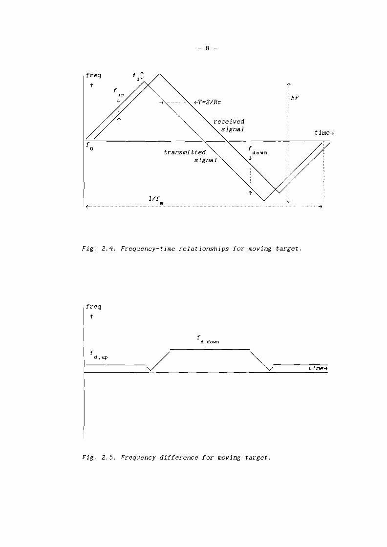
When the target is moving a Doppler frequency shift f is alsod

measured. The frequency difference is here (fig. 2.4 and fig.

2.5)

f = f - fup r d

f f + fdown r d

The range frequency f can be extracted by measuring the averager

frequency difference

f = 1 [f + f ]r 2 up down

The Doppler frequency is found by

f = .: [f - f ]d 2 up down

- 8 -

freq

l'

fo

lIfm

~T=2/Rc

...........~

Fig. 2.4. Frequency-time relationships for moving target.

freq

l'

fd,down

f /d, up

--time~

Fig. 2.5. Frequency difference for moving target.

- 9 -

When f is larger than f , the calculations of these frequenciesd r

are reversed. When sinusoidal modulation is used instead of a

linear modulation, the frequency difference is not constant over

a modulation cycle. By measuring the average frequency difference

the range frequency can be calculated.

One of the major applications of the FM-CW radar principle has

been as an altimeter on board aircraft to measure height above

the earth. The large target cross section and the relatively

short ranges permit low transmitter power and low antenna gain.

Since the relative motion, and hence the Doppler velocity between

the aircraft and ground, is small, the effect of the Doppler

frequency shift may usually be neglected.

2.2 Altimeter antenna isolation

As seen in fig. 2.3 the altimeter system uses two antennas. The

isolation between the transmi tting and the receiving antennas

must be sufficiently large to reduce the transmitter leakage

signal, which arrives at the receiver via the direct coupling

between antennas, to a negligible level.

The ARINC (Aeronautical Radio Inc.) requirements demand that the

RF isolation between the two antennas (transmit and receive) of

each system as installed should be at least 75 dB. A connection

between the transmit and receive antennas could be used to com-

pensate for a part of the direct antenna coupling. However this

is not allowed by ARINC in order to assure complete unit inter­

changeabili ty. In dual or triple radio altimeter installations

isolation between the transmitting antenna of one system and the

receiving antenna of all other systems should be 60 dB or more.

Isolation between transmit-to-transmit antennas of any two

systems and between receive-to-receive antennas of any two

systems should be 50 dB or more [4].

- 10 -

2.3 Altimeter antenna modeling

In the past the antennas used by Fokker for the radio altimeter

are horn antennas made by TRT. The horn antennas can be modeled

as slot antennas having the same dimensions and a TE field01

distribution on the aperture. The size of the slot representing

the horn antenna can also be chosen in such a way that the ra­

diation pattern of the horn antenna and the radiation pattern of

the slot antenna are the same.

The antennas presently used for the radio altimeter system are

microstrip antennas (Altimeter S67-2002-Series by Sensor Systems

Inc.). A rectangular microstrip antenna can be represented by two

radiating slots.

In this study only the horn antennas will be modeled. The actual

aperture dimensions are 0.90 A x 1. 54 A (assumed is here that

f = 4300 MHz). When we try to adapt the dimensions of a slot to

the radiation pattern of the horn antenna, the slot dimensions

become approximately 0.87 A x 1.32 A. These aperture dimensions

are larger than the dimensions of a slot with a TE -aperture01

field. For such a slot the smallest side should not be larger

than 0.5 A. The longest side should not be smaller than 0.5 A or

larger than 1 A. Standard "X-band" slots (0.305 A x 0.686 A) are

used to validate our software, by comparing wi th calculations

made by other authors [12,13,16,20,21,22].

- 11 -

3 MU11JAL COUPLING BETWEEN TWO SLOTS IN A CONDUCTING INFINITE

GROUND PLANE

In this chapter an expression is derived for the mutual

admittance between two rectangular apertures on a conducting

ground plane (based on a paper of Borgiotti [8]). The expression

for the mutual admittance is given in terms of the plane wave

spectrum of the aperture field. The derivation of the mutual

admi t tance is based on the Reaction Theorem [5]. An asymptotic

expression for the mutual admittance for large spacing of the

apertures is also established. The derived expression for the

mutual admittance can be used to calculate the mutual coupling

according to the network theory.

3.1 DEFINITION MUTUAL ADMITTANCE BETWEEN TWO SLOTS

The mutual admi t tance between two slots in a conducting ground

plane can be derived from the Reaction Theorem [5] [6]. The

Reaction Theorem is based on the reciprocity between two systems:

a response of a system to a source is unchanged when source and

measurer are interchanged. The Maxwell theory applied for two

sources a and b yield:

'iJ X H = jwcE + I 'iJ X H = jwcE + I (3.1a)a a e,a b b e,b

'iJ X E = -jwllH I 'iJ X E = -jwllH I (3.1b)a a m,a b b m,b

Based on (3.1a) and (3.1b) the fields of the two sources can be

related:

'iJ.(EXH -EXH)=E.I -H.I -E.I +H.I (3.2)a b b a b e,a b m,a a e,b a m,b

- 12 -

Consider a region V enclosed by a surface S containing these two

sources. Equation (3.2) can be rewritten as

II (E X Ii - EX Ii ). d~ =a b b a

5

+ H . I ) dVa m,b

(3.3)

This is called the Lorentz reciprocity theorem [6], [10]. For a

infinitely large region V enclosed by S the surface integrationlXl lXl

amounts to zero because of the far field properties of E and H:

rXE =ZHa 0 a

rXE =ZHbob

Combining (3.3) and (3.4) yields

(3.4a)

(3.4b)

lXl

IIL (E . I - H . Ib e,a b m,a E . I + H . I ) dV = 0

a e,b a m,b(3.5)

The integration in (3.5) can be reduced to the region containing

the sources. The integration extended to the entire space, except

for a region containing the sources, is zero, because no sources

are present in this region. This statement combined with (3.5)

yields that integration throughout any region containing the

sources will amount to zero:

E . I + H . I ) dV = 0a e,b a m,b

(3.6)

Dividing the region that contains all sources in a region that

contains the a sources and a region that contains the b sources,

(3.6) can be rewritten as

IIIy(Eb·le,aa

- Hb· 1m,a) dV = IIIy(Ea.le,bb

- H . I ) dVa m,b

(3.7)

- 13 -

The integrals in (3.7) have been given the name reaction. By

definition, the reaction of a field a on a source b is

<b,a> - H . I ) dVb m,a

(3.8)

which reduces (3.7) to

a

<b,a> = <a,b> (3.9)

Next the case of two radiating slots in a conducting infinite

ground plane will be considered. Each slot can be represented by

a magnetic current:

I =-(nXE)<Hz)m,a a

(3.10)

Equation (3.10) substituted in (3.7) yields for the left hand

term

<b,a> = III Ii. I dVy b m,a

a a

X E ) dSa

(3.11)

Source b is a vol tage source, which can be represented by a

magnetic current. The right hand term of (3.7) is written as

<a,b> = IIIy(Ea.le'bb

H . I )dV =a m,b

X E ) dSb

V Ib ba (3.12)

The combination of (3.11) and (3.12) yields

V Ib ba =

a

X E ) dSa

(3.13)

- 14 -

In equation (3.13) I is the current at source b due to a vol­ba

tage source at source a. The mutual admittance can now be defined

as

IY = ba =

12 Va

1

VVa b

(3.14)

Equation (3.14) is a stationary formula, i.e. little changes in

the field distribution have no effect on the value of the mutual

admittance [61, [81.

The choice of calculating the mutual admittance instead of cal­

culating the mutual impedance is caused by the use of voltage

sources. When electrical current sources are used the mutual

impedance can be defined. The voltage V in (3.14) is defined as

V = II E(x,y).e(x,y) dxdy (3.15)

is called the vector mode function.In equation (3. 15) e (x , y)

Assumed is here, that on the aperture only one mode (IE )01

exists. The E- and H-fields for a TE-field are defined as [6]:

Ee - e Ve= e

He = he Iet

(3.16a)

(3.16b)

V and I are called the mode voltages respectively the mode cur­

rents. The superscript e denotes the TE-field and the subscript t

denotes the tangential field on the aperture. For TM-fields

(superscript m) the relation is

~-m vn= e

t

j{ID = hm1

m

(3.17a)

(3.17b)

- 15 -

The mode vectors e and h are normalized such that

II 1ee 12

dS = II 1he 12

dS = 1

II lem l2

dS = II Ihm l2

dS = 1

(3.18a)

(3. 18b)

and the integration extends over the wave guide cross section.

The tangential E- and H-fields can be expressed as a summation

over all possible modes

E = L ~e ye + ~m yffitil iii

Because of the orthogonality relationship

II -e -me

1. e J dS = 0

Combination of (3.19a) and (3.19b) yields

(3. 19a)

(3. 19b)

(3.20)

II E .et i

dS = Yi

(3.21a)

II H . h dS = It i i

(3.21b)

3.2 MUTUAL ADMITTANCE FOR TWO IDENTICAL RECTANGULAR SLOTS

Consider two identical rectangular slots in an infinitely large

conducting ground plane (z=O). The two slots radiate in the half

space z~O and are both polarized in the same direction, which

means parallel to the short side of the slot. The distance

between the centers of the two slots is given by d. The direction

angle, given by ¢, is the angle between the displacement vector d

and the x-axis (fig. 3.1).

l'Y

slot A

d

- 16 -

slot B

~2a

Figure 3.1. Position of the slots.

For the above configuration equation (3.14) is written as

(3.22)

To calculate the mutual admittance the inner product of the

H-field caused by aperture B and the E-field caused by aperture A

has to be integrated throughout aperture A. First an expression

for the H-field caused by aperture B has to be found.

The two dimensional Fourier transforms in the xy-plane are

defined as

g (k •k )x y

1= 2n II e3.23a)

Eex.y)1= 2n II e3.23b)

- 17 -

The definition of these transforms for z*O is

-E(x,y,z) (3. 24a)

-g' (k ,k )

x y1 II -E( ) j(k x+k y+k z) dxdy= 2n XtY,Z e x y z (3.24b)

1 II - j(k x+k y) d dg'(kx,ky'z) = 2n E(x,y,z) e x y x y

Equation (3.23) and (3.24) yield

~ (E(X,y,O)) = g(k ,k ,z=O) = g(k ,k )x,Y x Y x Y

~ (E(X,y,Z)) = g'(k ,k ,z) =x,y x y

(3.24c)

(3.25a)

1II-E( ) j(kx+ky)2n x,y,z e x y dxdy =

The convolution is defined as

-g'(k ,k )

x y

-jk Ze z (3.25b)

g(x,y) • h(x,y) = II g(x' ,y') hex-x' ,y-y') dX'xy'

and the convolution in k-space is

(3.26a)

Combination of (3.23) and (3.26) yields

~(g(X,Y)h(X'Y)) = 21 ~(k ,k ) • H(k ,k )n x y x y

(3.27a)

(3.27b)

The E-field due to a magnetic current on aperture B is given by

E (x,y) = ! V X A (x,y)B £: m,B

(3.28)

- 18 -

A is the magnetic vector potential (in the half space z~O)m,B

given by

- C fff - e-jk~X-X' )2+(y_y' )2+(Z-z' )2A (x,y)=-- I (x',y',z') dV

m,B 2n V m,B II .222B (X-X') + (y-y') + (z-z' )

(3.29)

The magnetic current density

through

I is related to the E-fieldm,B

I (x' y' z')B ' ,m,

-= o(z') (E (x' y') X z)

B '(3.30)

The combination of (3.28) to (3.30) yields (for the half space

z~O)

E (r) = - 'iJ X- -

(E(r') X z) dr' (3.31)

The E-field in unbounded space is twice as small as the E-field

for a half space (3.31):

E(r) = - -(E(r') X z) dr'

In equation (3.31),r = (x,y,z) is a field point and

r' = (x' ,y' ,z') is a source point. The Fourier transform of

(3.31) is

1JJ-E( ) j(kx+ky+kz)g(kx,ky

) = 2n x,y,z e x y z dxdy =

(3.32)

- 19 -

This can be written as

2; II [v X ¢V] dxdy - 2; II [v¢ X v] dxdy

-In (3.33) ¢ and V are defined by

~ j(k x+k y+k z)¥' = e x y z

(3.33)

(3.34)

-(E(r') X z) dr' (3.35)

The term

-dxdy = f ¢V dC = a (3.36)

because, for fixed z, V as function of x and y becomes zero due

to the term

1

/ .2 2 2(x-x' ) +(y-y') +z

when the contour is chosen on infinity and by assuming some loss.

Combination of (3.34) to (3.36) yields

jk X 2; II ¢ V dxdy =

J'k X 1 II j(k x+k y+k z)2n e x y z- -

(E(r') X z) dr' dxdy

(3.37)

e-jklrl

Irlwritten as

- 20 -

The second integral is the convolution of the scalar function

~

and a vector function E(r) X z. Equation (3.37) can be

+jk ze z =

(3.38)

1In (3.38) ~(kx.ky) is substituted by jk (see appendix A).z

The Fourier transform of the H-field is found through the Maxwell

equations:

-1k X k X (f~(k .k ) X ;) 1

jk =jWj.L x y

z

1([k.{g(kx.ky) X ;}]k - k2g(k ,k ) X ;) (3.39)

j.Lwk x yz

The integration of the E-field due to aperture A and the H-field

due to aperture B extends to the aperture of slot A. Equation

(3.39) denotes the relation between the E-field and the H-field

at any point of the half space. When both slots are identical,

the mutual admittance can be expressed as a function of only the

E-field on the aperture of one of the slots. The H-field due to

aperture B is represented by the H-field due to aperture A

shifted over a distance d. Equation (3.14) can now be written as

Y (d) =12

1v-v- II H(x-dx·y-d ). (E(x.y) X z) dxdy

A B 5 YA

(3.40)

- 21 -

The Fourier transform of the shifted H-field is

1f(k .k )x y

j (k d + k d )e xx yy =

1

Ilwkz

(3.41)

According to (3.41) H(x-d .y-d ) can be written asx y

(Xl (Xl

H(x-dx,y-dy) = ;n_l_l Il~kz ([k·<gt(kx·ky)X;}]k

Equation (3.42) substituted in (3.40) yields

(3.42)

Y (d d) = - _1__1_ II (E(x,y) X z)12 x' Y V V 2nwll

A B SA

j (k d + k d) - j (k x+k y+k z) dk dk } d de x x y y e x y z X yx y

(3.43)

By interchanging the order of the integrations, and noting that

equation (3.43) can be written as

-g (-k .-k ) X z

t x Y(3.44)

- 22 -

(Xl (Xl

Y (d ,d ) =12 x y

1 1 II dk dkV V WjJ. x YA B --

k2 g (k ,k )XZt x Y

- ~

g (-k ,-k )XZ - k. (g (k ,k )XZ) k. (g (-k ,-k )XZ)t x y txy t x y

kz

j (k d +k d )e x x y y = (3.45)

The field in k-space is expressed in polar components through

-g (k ,k ) = g (k ,k )p + g~(k ,k )¢txy ppz 'l'pz

(3.46)

The propagation vector k is also transformed to polar coordinates

k = k p + k z (3.47a)p z

k2 k2 k 2 (3.47b)+

P z

k 2= k 2 + k 2 (3.47c)P x y

By writing g for g (-k ,-k) an g~ for g~(-k ,-k) we findp p x Y 'I' 'I' X Y

(3.48a)

and

(3.48b)

Subtraction of (3.48b) from (3.48a) yields

(3.48c)

- 23 -

Equation (3.45) can now be written as

Y (d, d )12 x y

1= 'TV

A B

co co k2g (k ,k )g (-k ,-k ) + k 2g~(k ,k )g~(-k ,-k )111 p x y p x y Z 'I' X Y 'I' X Yw~_ _ -----=------=---'--------;""k---'-z------'---'-------'-----'--

j(k (x-d )+k (y-d )) dk dke x x y y

x y(3.49)

De definition of the Fourier transform (3.24/3.25) shows that

•g (-k ,-k ) = g (k •k ) (3.50a)p x y p x y

•g (-k •-k ) = g</> (k ,k ) (3.50b)</> x y x y

•assuming E(x,y) = E(x,y). i.e. equiphase illumination. The

mutual admittance is then [8]

Y (d. d )12 x y

1= 'TV

A B

k =z

k = I k2-k 2_k i.z x y

Z ~ O. For the

j (k d +k d )dk dk = (3.51)e x x y y

x y

The integration in k-space over k and k extends from -co to +co.x y

For the region k 2+k 2::sk2 k is real and is given byx y z

These waves are propagating into the region

region k 2+k 2>k2, k is imaginary, given byx y z

j I k 2+k 2_ki

= - j Ik I and the waves are evanescent. Thex y z

imaginary k is chosen to be negative to keep the fields finitez

when k goes to infinity. The evanescent waves are propagating inz

- 24 -

a direction parallel to the aperture plane. The energy associated

with these waves is therefore tied to the aperture plane and is2 2 2stored there [7]. Integration over the region k +k ~k produces

x y

the real part of (3.51) and integration over the region

k 2+k 2~k2 produces the imaginary part (see appendix B):x y

1Y (d ,d ) = :-:-;--;---

12 x y V V WIJ.A B

+ k 21g'¢(k .k ) /2k Z x Y cos(k d )cos(k d ) dk dk

xx YY x YZ

2 2 2 2

JIk Ig' (k , k ) I -I k / Ig'A. (k ,k ) I

. pxy z'I'xy

+ J IkJk2+k >k2 z

x y

cos(k d )cos(k d ) dk dk }xx yy x y

(3.52)

3.3 ASYMPTOTIC EXPRESSION FOR THE MUTUAL ADMITTANCE

When d » A the far field expression for H can be used in (3.14).

The far field is reached for

- - 2 - - 2d»~or~» 1

A dA

The H-field in the point r-d is given by

(3.53)

H(r-d) (E(r') X z) dr' (3.54)

For d » A. V X can be replaced by d X. The vector d is the vector

with unity length in the direction of d. We can assume that

(3.55)

- 25 -

for the denominator of (3.54). This approximation cannot be used

for e-jklr-d-r' I. The argument can here be approximated by

(3.56)

Combination of (3.54), (3.55) and (3.56) yields

Define a scalar function ¢ and the vector function v

(3.57)

¢ = jkd. (r-r' )e (3.58)

-v = E(r') X z

For ~ X ¢v can now be written

~ X ¢v = ~ ¢ X v + ¢ ~ X v = ~ ¢ X Vr r r r

because v is independent of r. ~¢ can be written as

~¢ = ¢ ~(jkd. (r-r')) = ¢ ~(jkd.r) = jkd¢

Combining (3.60) and (3.61) yields

~ X ¢v = jkd¢ X vr

and

_ 2 A

~ X ~ X ¢v = -k d X d Xr r

Equation (3.57) can thus be written as

(3.59)

(3.60)

(3.61)

(3.62)

(3.63)

_k 2 e-jkldl A 1 II [ AJA ·kd (- -')H(r-d) = jw~ d X 21l E

t(r' ). d z e J . r-r dr' (3.64)

Idl

- 26 -

where d X (Et X z) = [Et(r,).d]; has been used.

Substituting (3.64) in (3.40) yields

Y (d) =12

2V \ II H(X-dx

, y-d ). (; X E(x, y)) dxdyA B 5 Y

A

= _1_ e- jk I d 1 2nk -!.II [E- ( ) d-] jk (d x+d y) d dj V V~ 2n t x,y. e x y x Y

A B 'I I '" I

1= j'TV

A B

-jkldle 2nk 8 (k ,k ).8 (-k ,-k )

7ll dl t x y t x y(3.65)

g is written in polar coordinates trough the transformation

x = p sinS cos¢>

y = p sinS sin¢>

z = p cosS

(3.66a)

(3.66b)

(3.66c)

The stationary phase method can be used to calculate the far

field in the half space z~O [7], [9], [11]:

According to the Maxwell theory k. g = 0 for all points in the

half space z~O. This implies that k g +k g +k g =0 orx x y y z z

g =z

sinScos¢> g + sinSsin¢> gx y

cosS

- 27 -

The far field as a function of g and g isx y

'k - jkrE = J e

r

{COSS gx + cosS gy - (sinScos</> g + sinSsin</> gy);}x y x

or in polar coordinates

E = jk e-jkr {e (g (k ,k )cos</> + g (k ,k )Sin</» +

r xxy yxy

</>cosS (-g (k ,k )sin</> + g (k ,k )cos</»}x x y y x y (3.67)

In the plane of the apertures (S=rr/2) the radiation pattern is

F(S,</» e (g (k ,k )cos</> + g (k ,k )Sin</» =x x y y x y

= e (g (k ,k )) = g (k ,k )p x y p x y

(3.68)

From (3.68) can be concluded that only the p-component of g isl

important in the far field. This could be predicted analyzing eq.

(3.51). The first term of the integrand has an integrable

singularity (for k =0) and will add the largest contribution toz

the integration. The second term of the integrand is regular.

Equation (3.65) becomes now

Y (d)12

'kldl1 e - J 2rrk - -= j v-v' --------- g (kcos</>,ksin</».g (-kcos</>,-ksin</»A B ~Idl p p

(3.69)

In (3.69) k and k are replaced by k.cos</> and k.sin</>, Assumingx y

that the phase is constant on the apertures the mutual admittance

is

1 e-jkldl2rrk - 2j v-v'~ Ig (kcos</>,ksin</» I

A B "1'"" I P(3.70)

- 28 -

3.4 MUTUAL COUPLING BETWEEN THE SLOTS

The calculated mutual admittance between two slots can be used to

calculate the mutual coupling between the slots. The system with

the two slot antennas will be considered to be a linear passive

microwave network. In this network the relations between the

voltages of the incident and the reflected traveling waves are

given by the scattering matrix S:

S12

S22

] [:[ ] (3.71)

+

~[

These network parameters are explained in fig. 3.2.

~ ~1

S S2

11 12

~ f f1~

s

S Syr 21 22 yr ~

~2

Fig.3.2. Network parameters.

The voltages in this network can be represented by a signal flow

graph (fig. 3.3). The voltage Y represents the contribution ofs

the source to v:. i.e.

yi = Y + f yr1 s s 1

(3.72)

ys S

21

f S Ss 11 22

S12

Fig.3.3. Signal flow graph.

- 29 -

From (3.71) two equations can be derived:

The reflection coefficient f 1 is defined as

and f is defined by (3.72) and bys

(3.73a)

(3.73b)

(3.74)

fs

2 -2S 0

=2 +2

S 0

(3.75)

Combination of (3.73b) and (3.74) yields

Vr S2 21=

Vi 1 - f S1 1 22

The relation between Vi and Vi is1 2

Vi vrf

1S212

f1

2= =

Vi Vi 1 - f lS221 1

Substitution of (3.77) in (3.73a) yields

(3.76)

(3.77)

(3.78)

- 30 -

From (3.72) and (3.78) the relation between Y and yr can bes 1

derived:

ys =

[5 +

115

12

r15 ]-121 _ r1 - r 5 s

1 22

(:).79 )

Finally from (3.76), (3.78) and (3.79) can be concluded

ys

yr yi yr2 1 1= - =

yi yr y1 1 s

512

1-5 r -5 r -5 r 5 r +5 r 5 r11 s 22 1 21 s 12 1 11 s 22 1

(3.80)

This relation could also be found by applying Mason's rules to

the signal flow graph of fig. 3.3. When both source and load are

matched to the network impedance, i.e.

(3.81)

the power coupling between source and load is proportional to the

square of the ratio of yr and Y :2 s

c =IY~12

\V 1

2

s

(3.82)

When condition (3.81) is substituted in (3.80), the power

coupling according to (3.82) is

The S and the Z matrix are related as

S = (Z - Z ) (Z + Z )-19 9

(3.83)

(3.84 )

Z is a diagonal matrix of which the elements are the9

characteristic impedances of the network waveguide. According to

(3.84) and assuming that Y =Y and Y =Y (due to the symmetry11 22 21 12

in the network) the scattering coefficient 5 is12

- 31 -

2 Z ZS = """'""=,--=-----:=-9::....,,-1.,..,2=--=-_ _=______

12 (Z +Z +Z ) (Z +Z -Z12)9 11 12 9 11

(3.85)

By applying Y = Z-l to (3.85) S12

can be written as

S =12

- 2 Y Y9 12

(Y +Y +Y HY +Y -Y )9 11 12 9 11 12

(3.86)

In (3.86) Y is the self admittance11

mutual admittance between the two

characteristic admittance of the

of the aperture, Y is the12

apertures and Y is the9

waveguide. The comparison

between the system of two radiating apertures and a two port

defined by admittances is illustrated by fig. 3.4.

Y9

Y Y11' 12

Y Y22' 11

Y9

Y9

Y -Y11 12

Y12

Y -Y22 12

Y9

referenceplane

referenceplane

Fig. 3.4. System of two radiating apertures represented by a

two port.

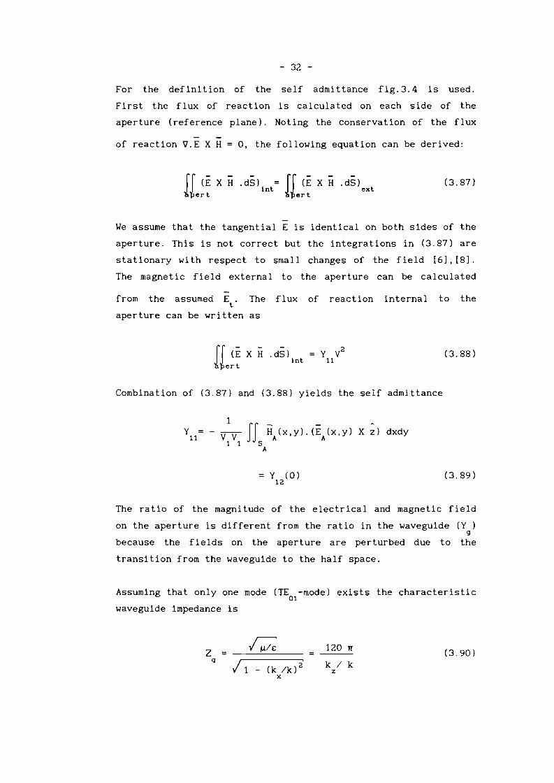
- 32 -

For the definition of the self admittance fig.3.4 is used.

First the flux of reaction is calculated on each side of the

aperture (reference plane). Noting the conservation of the flux

of reaction ~.E X H = 0, the following equation can be derived:

-X H .dS)

ext(3.87)

We assume that the tangential E is identical on both sides of the

aperture. This is not correct but the integrations in (3.87) are

stationary with respect to small changes of the field [61, [81.

The magnetic field external to the aperture can be calculated

from the assumed E. The flux of reaction internal to thet

aperture can be written as

-X H .dS)

Int(3.88)

Combination of (3.87) and (3.88) yields the self admittance

= Y (0)12

(3.89)

The ratio of the magnitude of the electrical and magnetic field

on the aperture is different from the ratio in the waveguide (Y )9

because the fields on the aperture are perturbed due to the

transition from the waveguide to the half space.

Assuming that only one mode (TE -mode) exists the characteristic01

waveguide impedance is

z9

=/ 1 - (k Ik) i

x

= 120 rr

k I kz

(3.90)

- 33 -

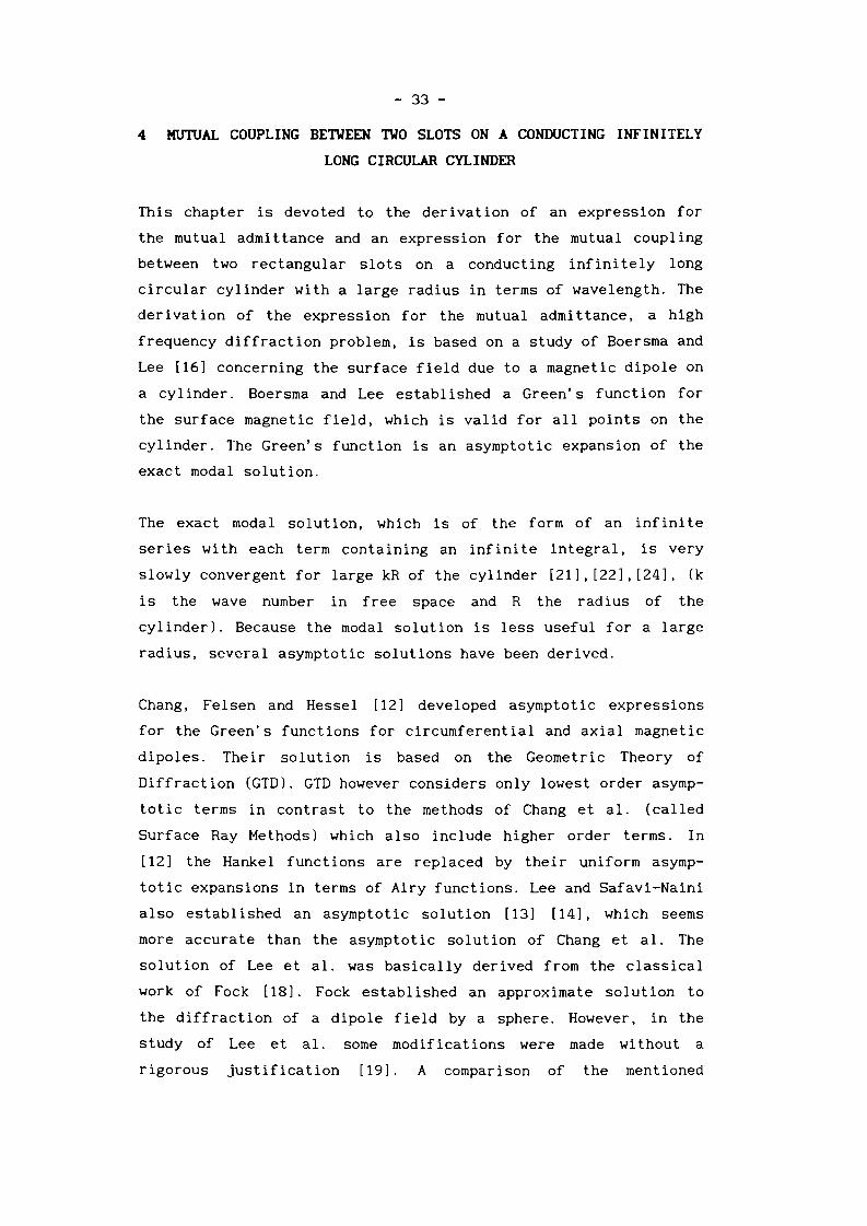
4 MUTIJAL COUPLING BETWEEN TWO SLOTS ON A CONDUCTING INFINITELY

LONG CIRCULAR CYLINDER

This chapter is devoted to the derivation of an expression for

the mutual admittance and an expression for the mutual coupling

between two rectangular slots on a conducting infinitely long

circular cylinder with a large radius in terms of wavelength. The

derivation of the expression for the mutual admittance, a high

frequency diffraction problem, is based on a study of Boersma and

Lee [16] concerning the surface field due to a magnetic dipole on

a cylinder. Boersma and Lee established a Green's function for

the surface magnetic field, which is valid for all points on the

cylinder. The Green's function is an asymptotic expansion of the

exact modal solution.

The exact modal solution, which is of the form of an infinite

series with each term containing an infinite integral, is very

slowly convergent for large kR of the cylinder [21], [22], [24], (k

is the wave number in free space and R the radius of the

cylinder). Because the modal solution is less useful for a large

radius, several asymptotic solutions have been derived.

Chang, Felsen and Hessel [12] developed asymptotic expressions

for the Green's functions for circumferential and axial magnetic

dipoles. Their solution is based on the Geometric Theory of

Diffraction (GTD). GTD however considers only lowest order asymp­

totic terms in contrast to the methods of Chang et al. (called

Surface Ray Methods) which also include higher order terms. In

[12] the Hankel functions are replaced by their uniform asymp­

totic expansions in terms of Airy functions. Lee and Safavi-Naini

also established an asymptotic solution [13] [14], which seems

more accurate than the asymptotic solution of Chang et al. The

solution of Lee et al. was basically derived from the classical

work of Fock [18]. Fock established an approximate solution to

the diffraction of a dipole field by a sphere. However, in the

study of Lee et al. some modifications were made without a

rigorous justification [19]. A comparison of the mentioned

- 34 -

asymptotic expressions can be found in [15].

Boersma and Lee [16] derived a more justified asymptotic solution

for the surface field due to a magnetic dipole on an infinitely

long cylinder whose radius is large in terms of wavelength.

Starting from the exact solution, they extracted a Green's func­

tion for the magnetic field, which is valid for all points on the

cylinder. Their study Justified predictions earlier made by Lee

et al. about the behavior of the field propagating along the

generator of the cylinder.

In this study we will use the Green's function established by

Boersma et al. who calculated the magnetic field on the cylinder

due to a radiating slot on the cylinder. This magnetic field is

used to derive an asymptotic solution for the mutual admittance

and the mutual coupling between two slots on the cylinder.

Finally an approximate, closed-form solution for the mutual

admittance is given.

4.1 ASYMPTOTIC EXPRESSION FOR THE SURFACE MAGNETIC FIELD

For the derivation of the mutual admittance, the magnetic field

on a cylinder due to a magnetic current on the cylinder is

needed. An exact modal solution for the surface magnetic field is

presented in [12]. When the contribution of creeping waves which

have travelled around the cylinder is neglected, the circum­

ferential component of the surface magnetic field due to a

circumferential dipole M = ~ is given by [12]:

(4. 1 )

where

(4.2)H(2) (k R)

v t

- 35 -

(4.3)

In (4.2) and (4.3) k = Jk2_k2'. kt z t

2 2imaginary when k >k. The magnetic fieldz

Is real when k2<k2 and negativez

term H;' denotes thec

TMz-contribution to the surface magnetic field, the term H</>"

denotes the TE -contribution to the surface magnetic field. Thez

contribution of creeping waves that have travelled around the

cylinder can be neglected, because of the exponential attenuation

of creeping waves [12).

The quotient of the Hankel function and its derivative in (4.3)

can be replaced by a Debye-type asymptotic expansion (for Ivl or

t large and t positive) (16) :

H(2) (t) jt t 3

O(~)v (4.4)- +H(2), (t) y{2_v 2'

22(t2- v2 )2

VV

The expansion for the quotient of the derivative of the Hankel

function and the Hankel function itself, as in (4.2), is the

reciprocal of the former equation:

H(2), (t)v

. r??t22Jvt--v-

t

t(4.5)

The above equations hold for t>lvl. When t<lvl the square root

y{2_v 2' passes into _j~2_t2'. The expansion is not valid for both

z and Ivl small. This is the case when we use (4.4) or (4.5) in

an integral like

-co

co H(2) (k a)

J v t

H(2), (k a)v t

e- jv</> dv

- 36 -

where k a is small due to k ~k. Judging by the numerical resultst z

in [16] the error in the approximation of the integral is not

large.

The magnetic field in point P due to a magnetic dipole in point Q

has to be calculated (see fig. 4.1). The parameter s is the

geodesic distance between point P and point Q along the cylinder.

The cylinder has a radius R. The surface ray makes an angle e

with the ~-direction.

Rz

s

Q -Iz

_I

Fig. 4.1. A surface ray from source point P to observation

point Q on an infinitely long circular cylinder.

Substi tution of the quotient of the Hankel functions by the

Debye-approximation (with v = k R) of (4.2) and (4.3) yields fory

the magnetic field terms H;' and H;":

- 37 -

(4.6)

(4.7)

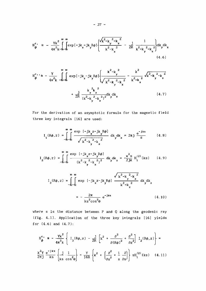
For the derivation of an asymptotic formula for the magnetic field

three key integrals [16] are used:

I (R<f>, Z)1

exp [-jk z-jk R<f>]

=-1-1 --/---2---Z-2--~Y2-' -- dkydkzk -k -k

y z

e- Jks

= 2njs

(4.8)

00 00

I (R<f>, z)2

exp [-jk z-jk R<f>J

=-1-1 ----(k-2-_-k-z-2-_-k--~-)-2- dkydkZ =

y z

(4.9)

I (R<f>, z)3

00 00

exp [-jk z-jk R<f>]z y

/ k2-k 2_k i___----:y:.....-__z_ dk dk

k 2 -k 2 y zz

=2n e- Jks (4.10)

where s is the distance between P and Q along the geodesic ray

(fig. 4.1). Application of the three key integrals [16] yields

for (4.6) and (4.7):

k2: e - j ks {--l _1_} _~ {k2 + (--.t + ! ~)} sH(2) (ks)

2nJ ks k 28

16R a2 a 1 (4.11)s cos s s s

- 38 -

== -

k2

y e-Jks {-.l _1} +

271j ks k 28s cos

. 28+ Sln

y { 2 2 a 2 . 2 1 a3

16k~ - cos 8 sin 8 as4 - (1 - 6cos 8s1n 8)~ as3

2 • 2 1 a2

+ (2 - 15 cos 8s1n 8)-- ---s2 as2

When we define

1 aD = S as

sH(2l (ks) (4.12)1

HC, and HC

" can be written asif> if>

k2y e- Jks

(k~1 ) -

k2y (2H~2l (kS))271j~ cos28 16kR

and

k2y - Jk. { .

c:s2.}H

C' •

e J== - 271j~ ksif>

Y {k2+ 2 }

e- jks

cos28 a . 2 1 a+ 271j ---2 + Sln 8 - --

~as s as

_ ~_s2D3 _ D2 _ 4 4 2 . 2} (2)s D cos 8s1n 8 sH1

(ks) =16k~

(4.13)

- 39 -

k2y - j ks (+ -l(2-3sin2e-__1___ ) + 1 (2-3sin2e) )e . 2

2Rj k5""" SIn eks cos2e k2s 2

k2y (H~2) (ks) - ~ H(2) (ks) + ksH(2) (ks) cos2e sin2e) (4.14)

16kR ks 1 3

where ksH(2) (ks) -4H (2) (ks) - ksH(2) (ks) 8 H(2) (ks)= + ks3 0 1 1

In (4.13) and (4.14) we have used a recurrence relation for

Bessel functions

B (ks) + B (ks)n-1 n+1

(4.15)

and a relation for the derivative of a Bessel function [23]

s aa B (ks) = n B (ks) - ks B (ks)s n n n+1

(4.16)

For large ks the Hankel functions can be replaced by their large

argument expansions [23]:

H(2) (ks)~ ~ e- jks eJR/4{1 + j_1_ _ 9 }o vI~ 8ks 128(ks)2

H(2) (ks)~ ~ - jks JR/4{1 . 3 15}1 vi~ je e - J-- + 2

8ks 128(ks)

H(2) (ks)~ ~ - jks e jR/ 4{1 .35 945 }2 - vi~ je - J-- -

8ks 128(ks)2

This yields for the H;' and the H;"

(4.17)

(4.18)

(4.19)

- j ks { . 1 1 1/2 ( . )}_e__ --.l + __ (~ks) e -.lR/4 2 + _J_ks k 2e 4kR 2 4kss cos

(4.20)

and

- 40 -

k 2 y -jks { . 1~ . _e___ sin2e + -l(2-3sin2e------) +

2nJ ks ks 2ecos

(4.21)

The sum of (4.13) and (4.14) yields

k2y - jks [He ~ e . 2e +¢ 2nj~ SIn

j 2 1 2 ]ks (2 - 3 sin e) + (2 - 3 sin e)k

2s

2

(4.22)

The second term represents the effect of the finite, but large,

radius of curvature of the cylinder. The first term is exactly

equal to the solution for H¢ due to a magnetic dipole M = ¢ on a

flat ground plane (planar solution).

The exact modal solution of the z-component of the surface

magnetic field due to an axial magnetic dipole is [12]

(4.23)

- 41 -

Application of the Debye-type approximation (4.4) to the magnetic

field component Ha in (4.12) yields:z

j2R

(4.24)

Using the key integrals I and I from (4.8) and (4.9) yields1 2

y

21lj {

2 ] - jks2 .2 a 21 ae[k + SIn e - + cos e - - -- +

a 2 a kss s s

The derivatives of (4.25) can be calculated using (4.16)

k2

y [ 2 (2) ---.!. H(2) (ks) (2) 4 ]16kR -2cos e H2 (ks) - ks 1 + ksH3

(ks) cos e (4.26)

We only need to calculate the He and Ha because the slots are<p z

identical and either axial or circumferential. The mutual

admittance between two slots was defined (3.14) as:

Iy = BA =

12 VA

When the slots are axial, the electric field on slot A is circum­

ferential directed. For the calculation of the mutual admittance

only the axial component of the magnetic field on slot A, due to

the radiation of slot B, is needed. When the slots are axial, the

- 42 -

magnetic current on slot B is also axial directed. When the slots

are circumferential, the magnetic current is circumferential and

only the circumferential component of the magnetic field is

needed. For the case that the slots are arbitrarily directed, an

expression for the axial magnetic field due to a circumferential

directed dipole and the circumferential magnetic field due to a

axial directed dipole should also be derived.

The approximations for H~ and Ha in (4.22) and (4.26) are onlyc z

valid for large kR and small ~, where [16]

~ = 2-1 / 3 ks cos4/38(kR)2/3

(4.27)

The surface magnetic field decays exponentially as a function of

~. For large ~, the behavior of the surface magnetic field is

properly described in terms of the Fock functions u(~) and v(~).

The Fock functions u(~) and v(~) are defined by [14]. [18]

jn/4 w (t)e-j~tdtv(~)

e ~1/2 Jw

2

, (t)2v'lT r 21

3jn/4~3/2

Jw2 ' (t)e-j~tdtu(~)

e=Vi r w

2(t)

1

(4.28)

(4.29)

The contour r is sketched in fig. 4.2. The function w is an1 2

Airy function

1 J 1 3w (t) = --- exp(tz - - z )2 Vi 3

n r2

The integration contour r is also sketched in fig. 4.2.2

(4.30)

- 43 -

1m t

r1

Re t

1m t

r2

Re t

Fig. 4.2. Integration contours rand r .1 2

The integrals containing the quotient H(2l (k R)/H(2l, (k R) shouldv t v t

be approximated by the hard Fock function v(~) and its deri-

vative. The integrals containing the quotient

H(2l, (k R)/H(2l (k R) should be approximated by the soft Fockv t v t

function u(~) and its derivative [16]. By closing the contour rat infinity, the Fock functions can be represented by a residue-

series

-jn/4 .;rr 00 exp [-j~t' ]

v(~) ~1/2 L n= e n ,tn=l n

2e jn/ 4 .;rr00

u(~) = ~3/2 L exp [-j~t ]n

n=l

(4.31)

(4.32)

Here t = It I e- jn/ 3 and t ' = It 'I e- jn/ 3 , where t and t • aren n n n n n

the zero's of w (t) and w • (t) (see appendix C).2 2

For small ~. the Fock functions can be represented by the

power-series expansions

- 44 -

v(~) 1vn j71/4~3/2 7j ~3 7vn e-j71/4~9/2 + O(~6) (4.33)- - 4 e + - +

51260

u(~) 1 vn j71/4~3/2 5j ~3 5vn e-j71/4~9/2 + O(~6) (4.34)- -2 e + - +

6412

To match (4.13) (4.14) and (4.26) to an expression containing the

Fock functions, we write

2 - jks [ ]He,,~ k Y _e C u(~) + D u' (~)f/> - 271j ks

k 2 y e - jks [ ]- 2nj~ E v(~) + F v' (~)

(4.35)

(4.36)

(4.37)

and replace the Fock functions and their derivatives by the

approximations for small ~

v(~) 1 vn ej71/4~3/2- -4

u(~) 1 vn ej71/4~3/2= -2

v' (~)3vn ej71/4~1/2- -8

u' (~)3vn ej71/4~1/2- - 4

(4.38)

(4.39)

(4.40)

(4.41)

Combination of (4.13) and (4.35) yields

(4.42)

2- 1/ 3J' (4 . 2 11 . 3 7' 2 187 )B-- 4/38 Sln 8 . 2 J ( Sln 8 . 2

8----"---- cos - 12s1n 8 + - - - + 64s1n(kR)2/3 3cos28 ks 4 12cos28

(4.43)

- 45 -

combination of (4.14) and (4.36) yields

c = j 1ks cos28

2- 1/

3j (. 1)

D = cos4

/38 12~S --2-

(kR)2/3 cos 8

and finally the combination of (4.26) and (4.37) yields

(4.44)

(4.45)

= 2 j( 2) 1E cos 8 + ks 2 - 3cos 8 +k

2s

2

2(2 - 3cos 8) (4.46)

2 -1/3 j 4/3 (11 2 • 7F = cos 8 -12COS 8 + --.1 (-

(kR)2/3 ks 6"2 187 2)---2- + 64COS 8) (4.47)

3cos 8

From the former equations can be concluded that the the circum­

ferential component of the magnetic field, due to a circumferen­

tial magnetic dipole is given by

3sin28 - _1 ) + 1_(2 - 3sin28l) v(~) +2 2 2

cos 8 k s

j 3+ -(- ­

ks 4(4.48)

The axial component of the surface magnetic field, due to a axial

magnetic dipole is thus given by

2 - 1 /3 j 4/3 (11 2 . 7 2 187 ) ]+ cos 8 -12cOS 8 + --.1(-_ - 2 + 64 cos

28) v' (~) (4.49)

(kR)2/3 ks 6 3cos 8

- 46 -

4.2 ASYMPTOTIC EXPRESSION FOR THE MUTUAL ADMITTANCE

To derive an asymptotic expression for the mutual admittance, the

magnetic field due to the radiation of a slot on the cylinder is

needed. Eq. (4.48) represents the Green's function for the

circumferential component of the surface magnetic field due to a

circumferential magnetic source and will be called g¢. Eq. (4.49)

represents the Green's function g for the axial component of thez

surface magnetic field due to an axial magnetic source.

First we will consider the case of two circumferential slots (see

fig. 4.3). The arc length of the slots is 2a, the axial length is

2b. The centers of the slots have a circumferential separation

R¢ and an axial separation z .o 0

l'z

slot B

R¢o

+b

-b

slot A

() ···················1·· ················y;;;R¢ ~

-a +a

Fig. 4.3. Two identical circumferential slots on a developed

cylinder.

- 47 -

The circumferential component of the surface magnetic field is

now

R¢ +ao

H;(y,z) = JR¢ -ao

z +bo

J I (y, z )m,B B B

z -bo

g~(y,z,y ,z ) dz dy'f' B B B B

(4.50)

When we assume that only one mode

aperture, the magnetic current is

(IE )01

is present on the

I (y,z)=I (y)=E(y)Xnm,B m,B B

(4.51)

From (3.14) the mutual admittance can now be calculated:

a b1

V V J JA B-a -b

R¢ +ao

E (y) JA A

R¢ -ao

z +bo

J Im,B(YB)

z -bo

g~ (y ,y ,z ,z ) dz dy dz dy'f' A B A B B B A A

(4.52)g~ (s, e) dz dy dz dy'f' B B A A

z +bo

JE (y )E (y )A A B B

z -bo

b R¢ +aoa1

V V J J JA B-a -b R¢ -a

o

=

In eq. (4.52) the electric field on the aperture of slot A is

given by

(4.53)

and the electric field on the aperture of slot B is

(4.54)

The mode voltages are V and V are defined by (3.15).A B

- 48 -

The distance s and angle e are defined as

s = / (Y -Y ) 2 + (z -z ) 2 'B A B A

(4.55)

e = arctan[ ZB-ZA]Y

B-Y

A

(4.56)

and the Green's function gef> is given by (4.48). Combination of

(4.52), (4.53) and (4.54) yields

Y (Ref> ,Z ) =12 0 0

Z +bo

Jcos(2: yA)cos(2: (YB-Ref>o))gef>(S,e)dZBdYBdZAdYAZ -b

o

b Ref> +aoa

1

-2ab J J J-a -b Ref> -ao

(4.57)

For two identical axial slots (fig. 4.4) the mutual admittance

can be calculated following the same procedure.

l'Z

slot B

Zo

slot A+b

() y=Ref> ~

-bt l'

-a +a

Fig. 4.4. Two identical axial slots on a developed cylinder.

- 49 -

The mutual admittance between two axial slots is

Y (R</>, Z ) =12 0 0

(4.58)

ZA)COS(Zlla (z -z »)g (s,8)dz dy dz dyBO z BBAA

z +bo

J cos(z:z -bo

a b R</> +ao

J J J1

-Zab-a -b R</> -ao

Here sand 8 are defined again by (4.55) and (4.56) and g (s,8)z

is given by (4.49).

4.3 APPROXIMATE ASYMPTOTIC EXPRESSION FOR THE MUTUAL ADMITTANCE

The expression for the mutual admittance in (4.57) and (4.58) can

be evaluated for large ks. An approximation method was

established by Lee et al. [17]. This method will be used in

combination with the Green's functions derived by Boersma [16].

When a TE aperture field distribution is assumed, the mutual01

admittance for two circumferential slots is given by

Y (R</>, z ) =12 0 0

a b a b1

-Zab J J J J cos(z: YA) cos (z: YB)g</>(t,a)dZBdYBdZAdYA-a -b- a -b

(4.59)

with

(4.60)

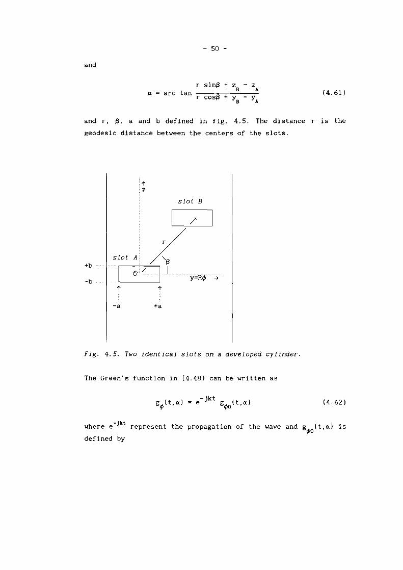
and

- 50 -

r sin(3 + z - ZB A(X = arc tan

r cos(3 + YB

- YA

(4.61)

and r, (3, a and b defined in fig. 4.5. The distance r is the

geodesic distance between the centers of the slots.

1"z

slot B

slot A+b

..•....... 1

0 /

-b1"

-a +a

Fig. 4.5. Two identical slots on a developed cylinder.

The Green's function in (4.48) can be written as

= -jkte g</>O(t,(X) (4.62)

where e-Jkt represent the propagation of the wave and g¢o(t,(X) is

defined by

- 51 -

k 2 y 1=

2nj kt

(j 1)kt --2-

cos <X

2-1 / 3 J' (4 . 2 114/3 SIn <X • 2u(~) + COS <X 2 - 12sIn <X

(kR)2/3 3cos <X

j 3+ -(- ­

kt 4(4.63)

and ~ is defined by

~ = 2-1/ 3 kt 4/3COS <X (4.64)

When the distance t 1s large with respect to the length of the

slots. t can be approximated by

() 2 ZA - Zs)2) 1/2t = (r cos~ + Y

A- Y

s+ (r sin~ +

YA-Ys Z -Z- r (1 + cos~ + sin~ ~)

r r(4.65)

-jktfor e ,and by r for g¢Q in (4.63). The direction angle <X in

g~o can be approximated by ~. The integration in (4.59) can now

explicitly be carried out. Due to the approximations the

integrals in (4.59) become Fourier transforms of the electric

field, where the integration is reduced to the aperture. The

result 1s

-1 22ab (2nab)

{

cos(ka cos~) }2 {Sin(kb Si~)}2 =

(;)2_(ka COS~)2 kb sin~ g~

32:b S2(kb sin~) C2(ka cos~) g~(r,~)n

(4.66)

- 52 -

where sex) and C(x) are defined as

sex) = sin (x)x

(4.67)

C(x) = (4.68)

The mutual admittance for two identical axial slots can be

approximated in the same way, which yields:

(4.69)

where g (r,~) is the Green's function given by eg. (4.49).z

This approximation holds for large kR and large kr.

4.4 MUTUAL COUPLING BETWEEN THE SLOTS ON THE CYLINDER

Although the geometry of the slots on the cylinder is different

from the slots on the ground plane, the coupl ing between the

slots can be calculated in the same way as in section 3.4, fol­

lowing the two-port network representation. Because the slots are

small compared to the radius of the cylinder, the self admittance

of the slots will be taken equal to the self admittance of a slot

in a ground plane.

- 53 -

5 NUMERICAL RESULTS

This chapter deals with the numerical results of the computations

of the mutual coupl ing between two slots on a ground plane and

between two slots on a cylinder. Two computer programs have been

developed for computations on a ground plane and two programs for

computations on a cylinder.

5.1 DESCRIPTION OF THE PROGRAMS

In this section the programs developed will be discussed. The

programs and subroutines can be found in appendix E.

5.1.1 Asymptotic method for the calculation of mutual coupling

between two slots on a conducting infinite ground plane (HeA).

The asymptotic formula for the mutual admittance is described in

chapter 3.3. The expression for the mutual admittance (eq.

(3.70)) is valid for a large distance between the slots (in terms

of wavelength). In addition to the restrictions concerning the

distance between the slots there is also a restriction to the

position of the slots. The expression is not valid for ¢ = 900

(H-plane coupling). For this case, g in (3.70) becomes zero duep

to the relation

g = g cos¢ + g sin¢p x y

wi th ¢ defined in fig. 3.1, and g equal toy

because the slots are assumed to be small.

the electrical field is equal to (see (4.53))

(5.1)

zero. g is zeroy

For small slots

(5.2)

- 54 -

so g isx

K sin(k a)g = V ab

2x

x k ax

cos(k b)y (5.3)

Although the magnetic field in the H-plane becomes very small for

large distances, it is not equal to zero. This restriction is a

resul t of the far field approximation. The programname is l1GA.

Because l1GA uses no integration routines, it is very fast. l1GA

uses the subroutine SELFADl1I, which calculates the self admit­

tance of the aperture. Subroutine SELFAD111 will be discussed at

the end of section 5.1.2.

5.1.2 Fourier transform method for the calculation of mutual

coupling between two slots on a conducting infinite ground plane

(11GB).

Eq. (3.52) is used to calculate the mutual coupling between two

slots, according to Borgiotti's Fourier Transform method. g andp

g are given by (5.1) and (5.3). Because of the symmetry proper-x

ties of the integrals in (3.52), the integration can be reduced

To avoid

open type is used (mid-

a singularity.

to one quadrant and the result multiplied by four. As can be seen

in (3.52) the integration over k2+ k2 :s k2 produces the real

2 2x Ipart and integration over k + k ~ k produces the imaginary

x y

the border between those regions, given bypart of Y At12

k2+ k2 = k2 or k =0, the integrand has

x y z

this singularity an integration rule of

point-rule). To decrease the step size in the neighborhood of the

singularity a coordinate transformation to polar coordinates is

used, as suggested in [20]:

kx

- 55 -

= k~ cos(nt/Z) (5.4)

k = k~ sin(nt/Z)y

where rand t range from 0 to 1, and for k2+ k2

~ k2

x y

(5.5)

kx

ky

= k~ cos(nt/Z)

= k~ sin(nt/Z)

(5.6)

(5.7)

where r ranges from 0 to infinity, and t ranges from 0 to 1. For

both regions dk dk can be written asx y

For

and for

k2+ k2 :s k2

:

k~ + k~ ~ k2

x y

dk dk = -x y

dk dk =x y

rdr dt

rdr dt

(5.8a)

(5.8b)

For numerical evaluations the integration in k space must bet

limited. The extent of the region over which must be integrated

in k space depends on the aperture size. The larger the aper-t

ture, the faster the function to be integrated approaches zero.

The separation of the slots is of influence on the integration

step size. The larger the separation, the more the integrand

oscillates, so the more samples have to be taken (reduction of

step size). For large separations of the slots, the calculation

time increases due to the reduction of the step size.

Because of the large calculation time for a large distance

between the slots, this program (nCB) is less suited for

engineering applications. The self admittance can be calculated

by using this method and setting the distance between the slots

to zero (subroutine SELFADnI). In nCB a subroutine (INPUTB) is

used to prov ide and change the va 1ue of the parameters. For

the calculations in 5.3 with nCB, the number of integration

intervals in r (see program in appendix E) was taken equal to

300, and the number of integration intervals in t ZOO.

- 56 -

5.1.3 Asymptotic method for the calculation of mutual coupling

between two slots on a conducting infinitely long cylinder (HGG).

For the mutual coupling calculations, according to the asymptotic

method, eq. (4.57) and (4.58) have been used (program HGG). The

Green's functions used in the program are given by eq. (4.48) for

circumferential slots and eq. (4.49) for axial slots (subroutine

PHIB and GZB).

In the subroutines PHIB and GZB provisions have been taken for

the case S = n/2, when the 1/ (cosS. cosS) terms can be removed.

For R very large (in our subroutines: R ~ 1. DE8) the planar

solution is calculated.

The Fock functions v(E;), v' (E;), u(E;) and u' (E;) are implemented in

the subroutines V, VA, U, and UA. For small E; (E; ~ 0.7) the Fock

functions are calculated by the power-series expansions of eq.

(4.33) and (4.34). For large E; (E; > 0.7) the Fock functions are

approximated by the residue series (eq. (4.31) and (4.32)) with

the first ten terms. The crossover point E; =0.7 is chosen accor-o

ding to [14], to have a smooth crossover between the two repre-

sentations. For the calculations in this report, the aperture is

divided in 24 x 4 subdivisions for the integration of the field

on the aperture. The subroutine INPUTG is used to provide and

change the value of the parameters. The subroutine SELFADNI

calculates the self admittance.

5.1.4 Approximate asymptotic method for the calculation of mutual

coupling between two slots on a conducting infinitely long

cyl inder (HGD).

The program HGD calculates the approximate mutual coupling be­

tween two slots on a cylinder according to eq. (4.66) and (4.69).

The Green's functions and Fock functions used for HGD are the

same as for HGG. Two extra subroutines, SN and GN, are provided

for the functions S(x) (eq. (4.67)) and C(x) (eq. (4.68)). The

input parameters are provided by subroutine INPUTD and the self

admittance is calculated by SELFADHI.

- 57 -

5.2 VALIDATION OF THE PROGRAMS

The developed programs have been validated by comparison of our

calculations with calculations and measurements performed by

other authors. First we will compare our results with calcu­

lations and measurements on a ground plane. The programs HCA and

HCB are validated by measurements and calculations in [20) (see

fig. 5.1). Some values for the mutual coupling at a distance of 1

wavelength are given in table 1 and can be checked in fig. 5.1.

The same calculations have been made with HCC and HCD for a

cylinder with R ~ 00 (ground plane)

Table 5.1. Hutual coupling (dB) for d = 1 A.

¢ HCA HCB HCC HCD

0.0° -19.4 -19.8 -19.6 -19.5

22.5° -21. 4 -21. 4 -21. 2 -21. 5

45.0° -27.9 -26.2 -26.0 -27.6

67.5° -40.2 -32.2 -31. 1 -34.0

90.0° -33.0 -33.0 -34.5

40

CD...

15

, FREQUENCY' 90 G~l

I-CALCUL.ATIONS F~EE SPACE,0 lI£ASUREO 18· 9Q' I '

: li. WEASUREO 13' 45'1

... YEASUREO i 3' 0' I

10 6~-"'7-----!:-~ ----::9--:':'IC---..,;~--:l12

SEPARATION (kd)

Fig, 5,1. Isolation between two slots (0.305 A x 0.686 A) (20).

- 58 -

Comparison of table 5.1 with fig. 5.1 shows that the results of

the programs MGB, MGG and MGD agree very well with the measure­

ments in [20]. The results of MGA show some deviation for ¢ near

900•

The programs MGG and MGD have been validated by calculations and

measurements for slots on cylinders. The mutual admittance cal­

culated by the programs MGG and MGD has been compared with re­

suI ts from [12], [13] and [16] (see table 5.2 and table 5.3). As

can be seen, the results of program MGG agree very well with the

exact modal series solution. The results of program MGD also

correspond reasonably well with the exact solution, except for

the phase in the case of H-plane coupling, which may be caused by

the relative short distance between the slots.

Table 5.2. Mutual admittance for ¢ =0, R = 1. 5171 .\, circum­o

ferential slots: 0.305 x 0.686 .\ (E-plane coupling). Magnitude in

dB. Phase in degree.

Exact Asymptotic Approx.

z (.\)o

0.381

1.524

6.096

12.192

30.480

[16 ]

- 62.62

720

- 71. 78

-1170

- 81. 84

340

- 86.48

40

- 91. 95

-1150

Chang

[12 ]

- 61. 70_ 68 0

- 70.96

-118 0

- 80.80

34 0

- 85.26

4 0

- 90.83

-112 0

Lee

[13]

- 62.54_ 72 0

- 71. 66

-116 0

- 81. 83

37 0

- 86.60

1 0

- 92.46

-110 0

Boersma

[16]

- 62.41_ 73 0

- 71. 84

-119 0

- 82.18

30 0

- 86.96

9 0

- 92.77

-120 0

MGG

- 62.43_ 73 0

- 71. 60

-116 0

- 81.77

37 0

- 86.55

1 0

- 92.41

-119 0

MGD

- 60.70_ 76 0

- 71. 43

-113 0

- 81. 85

38 0

- 86.66

o 0

- 92.55

-109 0

- 59 -

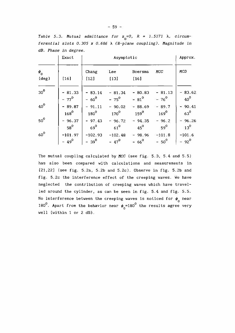
Table 5.3. Mutual admittance for z =0, R = 1.5171 A, circum­°ferential slots 0.305 x 0.686 A (H-plane coupling). Magnitude in

dB. Phase in degree.

Exact Asymptotic Approx.

cf>o

(deg) [16]

- 81. 33

- 77°

- 89.87

168°

- 96.37

58°

-101.97

- 49°

Chang

[12]

- 83.14

- 60°

- 91. 11

180°

- 97.43

69°

-102.93

- 39°

Lee

[13]

- 81. 34

- 75°

- 90.02

170°

- 96.72

61°

-102.48

- 47°

Boersma

[16]

- 80.83

- 81°

- 88.69

159°

- 94.35

45°

- 98.96

- 66°

MCC

- 81. 13

_ 76°

- 89.7

169°

- 96.2

59°

-101.8

- 50°

MCD

- 83.62

40°

- 90.41

63°

- 96.26

13°

-101. 6

- 92°

The mutual coupling calculated by MCC (see fig. 5.3, 5.4 and 5.5)

has also been compared with calculations and measurements in

[21,22] (see fig. 5.2a, 5.2b and 5.2d. Observe in fig. 5.2b and

fig. 5.2c the interference effect of the creeping waves. We have

neglected the contribution of creeping waves which have travel­

led around the cylinder, as can be seen in fig. 5.4 and fig. 5.5.

No interference between the creeping waves is noticed for cf> near°180°. Apart from the behavior near cf> =180° the results agree very

°well (within 1 or 2 dB).

_TOr

-60

~:l~ -3O~;:Z:::bf"

-20

-10

- 60 -

I FREQUENCY' 90GH, jI-THEORY: a IlEASUREIlENTS, '0 ' 10.1600'

i a. MEASUREMENTS, 10: 762cm

! 0 MEASUREMENTS, lO ~ S08c""~-~-_._----~

I°0'-----,2:':-O--4~0--W--IlO--'OO----:'20

¢o' "q

Fig. 5.2a. Mutual coupling for circumferential slots on cylinder

(0.305 A x 0.686 A). z = 3.048 A, 2.286 A, 1.524 A. R = 1.5171 A [22].o

-20

- iOu:--JO:::---:-:;;:;:-----:;J()::---~i'J-~5C:-----,;Q::::-----,-J2.C

1J,. Jeo

Fig. 5.2b. Hutual coupling for axial slots on cylinder (0.305 A x

0.686 A). Z = 1.143 A. R = 1.5171 A [22].o

- 61 -

70;-----,---~---------___:_--___,

i FRECUENCY' 90 "Hz60 , zo '0, '0' I 991 ,n, J' 0400 in, b' 0900 ,n

~50

~~ 40....o~

~30<l

Q,

~ 20

10

---- --------i '~EE SPACE-- ~UMERICAL iNTEGRATION i

! -- - RESIDUE SERIES APPROX I

, - - ~ANE CALCULATIONS

o0L-----:..30---5~O--9(-,----"2-0--,~50""'--""'8'::""0---:::'210'

ANGULAR SEPARATION, a.g

Fig. 5.2c. Mutual coupling for axial slots on cylinder (0.305 A x

0.686 A) Z = O. R = 1.5171 A [211.o

5.3 CALCULATIONS

The following calculations have been performed in order to study

the behavior of the coupling of altimeter horn antennas. Two

different slot sizes have been used in the calculations:

standard X-band slots: 0.305 A x 0.686 A (for validation

purposes), and

- "altimeter" slot antennas: 0.87 A x 1.32 A.

The radius of the cylinder is taken equal to the the radius of

the fuselage of a Fokker 100. The radius of the fuselage is

1. 65m, Le. 23.65 A (f = 4.3 GHz). Because the asymptotic for­

mulas are valid for a radius of 1.5171 A (see chapter 5.2), they

are certainly valid for a radius of 23.65 A. For calculations on

ground planes the radius is 109A (R ~ 00).

- 62 -

Calculations MGA

2 A- ::s d ::s 15 A-

¢ = 00

, 22.50

, 450

, 67.50

See respectively fig 5.6 and fig. 5.7. for the standard X-band

slots and for the "altimeter" slots.

Calculations MGB

o ::s d ::s 5 A-

¢ = 00, 22.50

, 450, 67.5

0, 900

See respectively fig 5.8 and fig. 5.9.

Calculations MGG

R = 23.65 A-

axial slots:

Calculations MGD

R = 23.65 A-

axial slots:

¢ = 0az = 0

a

2 A- ::s

2 A- ::s

z ::s 15 A-a

R¢ ::s 15 A­a

¢ = 0a

z = 0a

2 A- ::s

2 A- ::s

z ::s 15 A-a

R¢ ::s 15 A­a

circumferential slots:

¢ = 0 2 A- ::s z ::s 15 A-a a

z = 0 2 A- ::s R¢ ::s 15 A-D a

See respectively fig. 5.10

and fig. 5. 11 .

Calculations MGD

contour plots for axial slots:

R = 23.65 A-

circumferential slots:

¢ = 0 2 A- ::s z ::s 15 A-D D

Z = 0 2 A- ::s R¢ ::s 15 A-a a

See respectively fig. 5.12

and fig. 5.13.

contour plots for eire. slots:

R = 23.65 A-

2 A- ::s z ::s 15 A- 2 A- ::s z ::s 15 A-a a

2 A- ::s R¢ ::s 15 A- 2 A- ::s R¢ ::s 15 A-D a

See respectively fig. 5.14 See respectively fig. 5.15

and fig. 5.16. and fig. 5.17.

- 63 -

:s z :s 15 I- 2 I- :s z :s 15 I-0 0

:s R¢ :s 15 I- 2 I- :s R¢ :s 15 I-0 0

respectively fig. 5.18 See respectively fig. 5.19

contour plots for axial slots:

R = 109I-

2 I­

2 I-

See

and fig. 5.20.

Calculations NeD

axial slots:

contour plots for eire. slots:

and fig. 5.21.

¢ = aoz = ao

2 I- :s z :s 15 I­o

2 I- :s R¢ :s 15 I­o

circumferential slots:

¢ = a 2 I- :s z :s 15 I-0 0

z = a 2 I- :s R¢ :s 15 I-0 0

See fig. 5.22.

From fig. 5.6 it can be concluded, for the coupling between

standard X-band slots on a ground plane, that the isolation

increases as the separation of the slots increases. Furthermore,

the isolation increases as ¢ increases. For the case ¢ = a (E­

plane coupling) the isolation increases by 6 dB when the distance

between the slots is doubled. According to the asymptotic formula

(see fig. 5.6) the isolation increases for all ¢ by 6 dB for a

doubling of the separation. However the Fourier transform method

(fig. 5.7) shows that for ¢ = 900 (H-plane coupling), the in­

crement in isolation is 12 dB when the distance between the slots

is doubled. This behavior for the H-plane coupling is also shown

by the calculations on a cylinder with an infinite radius (ground

plane). See fig. 5.22. The planar solution of the Green's

function for circumferential slots is (see eq. 4.48):

(5.9)

- 64 -

For large distance sand e = 0 (H-plane coupling)-2

g ~ S¢

for large distance sand e = n/2 (E-plane coupling)-1

g ~ S¢

(5.10)

(5.11)

For large s the mutual coupling is proportional to the square of

the mutual admittance, and the mutual admittance is proportional

to the Green's function.

For the coupling between "altimeter" slot antennas on a ground

plane, the isolation increases as the separation increases.

However, the isolation for ¢ = 0 is larger than for ¢ = 22.5°.

The contour plots of fig. 5.20 and fig. 5.21 also show this

behavior.

In fig. 5.10 and fig. 5.11 the difference in isolation can be

seen for E-plane coupling between two circumferential (¢ =0) and°between two axial slots (z =0). The same holds for the H-plane

°coupling between two circumferential slots (z =0) and between two°axial slots (¢ =0).

°For the X-band slots the results of the asymptotic method (fig.

5.10) and the approximate method (fig. 5.12) agree very well. For

the "altimeter" slot antennas the asymptotic method (fig. 5.11)

and the approximate method (fig. 5.13) agree only for a large

separation of the slots. This is caused by the fact that these

slots are no longer small in terms of wavelength. When the radius

of the cylinder goes to infinity (planar solution) the difference

in E-plane isolation for circumferential slots and circum­

ferential slots disappears (fig. 5.22). This also holds for the

H-plane isolation.

- 65 -

The influence of the finite radius of the cylinder is shown by

the contour plots for the X-band slots (fig. 5.14, 5.15) and for

the ~altimeter~ slot antennas (fig. 5.16, 5.17). Within the

square of 15A x 15A on the surface of the cylinder, the largest

isolation can be found for the H-plane coupling between circum­

ferential slots.

When the radius of the cylinder goes to infinity the contour plot

for the circumferential slots becomes the same as the contour

plot for axial slots (mirrored in the line z = R¢ ).o

Our calculations for the ~altimeter" slot antennas can be

compared with measurements of mutual coupling between two alti­

meter horn antennas on a fuselage of an aircraft [25]. The

measurements are performed on a part of a cylinder with a radius

of R = 23.65 A. Table 5.4 shows measurements and calculations.

Table 5.4. Comparison of measurements and calculations of mutual

coupling on a cylinder (R = 23.65 A, ~ = 0).o

distance (z )o

7.6 A

11.9 A

measurement

- 76.3 dB

- 80.9 dB

NCC

92.9 dB

- 101. a dB

The difference in the value of the isolation measurements for d =7.6 A and d = 11.9 A is 4.6 dB, which corresponds with an

attenuation of 7.1 dB for a doubling of distance. Our calcula­

tions show a difference of 8.1 dB which corresponds wi th an

attenuation of 12 dB for a doubling of distance.

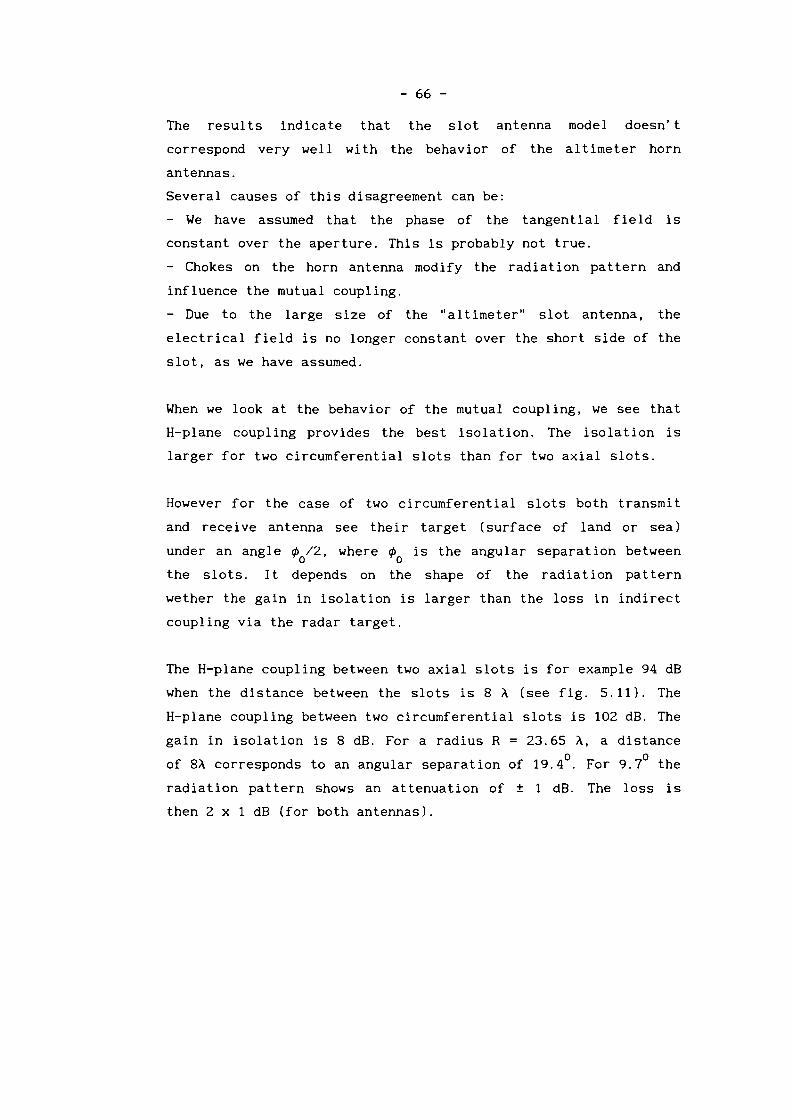
- 66 -

The results indicate that the slot antenna model doesn't

correspond very well with the behavior of the altimeter horn

antennas.

Several causes of this disagreement can be:

- We have assumed that the phase of the tangential field is

constant over the aperture. This is probably not true.

- Chokes on the horn antenna modify the radiation pattern and

influence the mutual coupling.

- Due to the large size of the "altimeter" slot antenna, the

electrical field is no longer constant over the short side of the

slot, as we have assumed.

When we look at the behavior of the mutual coupling, we see that

H-plane coupling provides the best isolation. The isolation is

larger for two circumferential slots than for two axial slots.

However for the case of two circumferential slots both transmit

and receive antenna see their target (surface of land or sea)

under an angle ¢ /2, where ¢ is the angular separation between° °the slots. It depends on the shape of the radiation pattern

wether the gain in isolation is larger than the loss in indirect

coupling via the radar target.

The H-plane coupling between two axial slots is for example 94 dB

when the distance between the slots is 8 A (see fig. 5.11). The

H-plane coupling between two circumferential slots is 102 dB. The

gain in isolation is 8 dB. For a radius R = 23.65 A, a distance

of 8A corresponds to an angular separation of 19.4°. For 9.7° the

radiation pattern shows an attenuation of ± 1 dB. The loss is

then 2 x 1 dB (for both antennas).

o

-10

-20 -

MUTUAL COUPLING SLOTS ON CYLINDER-10

-20

-30

MUTUAL COUPLING SLOTS ON CYLINDER

-30

-40

~

'" -50~8u

i -60

- - --40 -

-50o

-70 o 20 40 60 80 100 120-80 o 20 40 60 80 100 120 140 160 180

ANGULAR SEPARATION (DEGI ANGULAR SEPARATION (DEGI

zo • 3.0.8 LAMBDAZO • 2.296 LAMBDAZO • 1.52. LAMBDA

Figure 5.3.

SLOT DIMENSIONS: 0.305 X 0.696 LAMBDACIRCUMFERENTIAL SLOTSRADIUS OF CYLINDER 1.5111 LAMBDAASYMPTOTIC METROD (PROGRAM MCCI

ZO • 1.1.3 LAMBDA

Figure 5.4.

SLOT DIMENSIONS: 0.305 X 0.696 LAMBDAAXIAL SLOTSRADIUS OF CYLINDER 1.5111 LAMBDAASYMPTOTIC METROD (PROGRAM MCCI

- 68 -

MUTUAL COUPLING SLOTS ON CYLINDERO,------,.-----,----.,-----,....----,----,.....------r-----,---l

I-10 1-- -+--~----!--+----'---- r---'+--j

-J---+-1 -"-<--.---+-----+1.__--~--I-I-----t--jI ,!

iii :-30 --i--j---~---t-__T_---:------_+__I_1- ----·1

! I

iii I

-40h--

- I I I! I , I

~-50I- I:... l

§ I I

~ l

::> Ii -60 f--------1-------1----l---+---+---+---+----+---'~_i

-70 __---'-__---I-__-'--__..l...-__.l....-_---'__----'-__---I-__

o 20 40 60 80 100 120 140 160 180AJGtJI.Al SEPARATION [DEG)

%0 • 0.0 LAXBDA

Figure 5.5.

SLOT DIMENSIONS: 0.J05 X 0.686 LAMBDAAXIAL SLOTSRADiOS or CYLINDER 1.5171 LAXBDAASYMPTOTIC METHOD (PROGRAM MCCl

-20MOTUAL COUPLING SLOTS ON GROUNDPLANE

-40MUTUAL COOPLING SLOTS ON GROUNDPLANE

---80

-60

. .... .

"-".; --.~~--=;:L--

"-.----

-30

-50

-60 - --70

-90

§ -80

B

i

~-100

§§

I-120

Figure 5.6.

SLOT DIMENSIONS: 0.305 X 0.686 LAMBDAASYMPTOTIC METHOD (PROGRAM MCAI

SLOT DIMENSIONS: 0.810 X 1.320 LAMBDAASYMPTOTIC METHOD (PROGRAM MCAI

Figure 5.7.

14121086DISTANCE (LAMBDA)

0.0 DEG22.5 DEG45.0 DEG61.5DEG

421412108DISTANCE (LAMBDA)

6

0.0 DEG22.5 DEG45.0 DEG61.5 DEG

4-100

2

oMUTUAL COUPLING SLOTS ON GROUNDPLANE

oMUtUAL COUPLING SLOTS ON GROUNDPLANE

-20

-40

-60

~~::1~0u -80

I

-100 o 1 2DISTANCE (LAHIlDA)

-20

"-40.

- .

--.-- ~~ .. _---- -60-- --- ---

~~

-80

~

~8-100u

~-120

3 4 5 0 1 2DISTANCE (LAHIlDA)

~--~

3

- . - ..._---

--

4

- .. - ..---.-

---

5

-.JoI

0.0 DEG22.5 DEG45.0 DEG61.5 DEG90.0 DEG

SLOT DIMENSIONS: 0.305 X 0.686 LAMBDAFOURIER TRANSFORM METROD (PROGRAM MCB)

Figure 5.8.

0.0 DEG22.5 DEG45.0 DEG61.5 DEG90.0 DEG

SLOT DIMENSIONS: 0.81 X 1.32 LAMBDAFOURIER TRANSFORM METROD (PROGRAM MCB)

Figure 5.9.

-20

MUTUAL COUPLING SLOTS ON CYLINDER-40

MUTUAL COUPLING SLOTS ON CYLINDER

- -.........;, ---.------•._-;--

'--. '-.~-

'. .'.'.

-60

--.--.'--.~-

-40

-50------- -- -_._---

-80

-60 I

-.l.....

-70

~~-100

C>C> ~~ -80§ §

~ ............ I-90 -120

-1002 4 6

DISTANCE (LAMBDA)

8 10 12 14 2 4 6DISTANCE (LAMBDA)

8 10 12 14

AXIAL SLOTS PHIO-OAXIAL SLOTS 10-0CIRC. SLOTS PHIO-OCIRC. SLOTS 10-0

SLOT DIMENSIONS: 0.305 X 0.686 LAMBDAR: 23.65 LAMBDAASYMPTOTIC METHOD (PROGRAM MCC)

Figure 5.10.

AXIAL SLOTS PHIO-OAXIAL SLOTS 10-0CIRC. SLOTS PHIO-OCIRC. SLOTS ZO-O

SLOT DIMENSIONS: 0.81 X 1.32 LAMBDAR: 23.65 LAMBDAASYMPTOTIC METSOD (PROGRAM MCC)

Figure 5. 11.

-20MUTUAL COUPLING SLOTS ON CYLINDER

-40MUTUAL COUPLING SLOTS ON CYLINDER

-30

-40

~- '--. .--.'"'----- .. -......- ...

-60

~- '--. .-.'-.

-80

. .-50

-60

-...-70 f\.

~-100

,~<lI

~~ -80~ ~0 0u u

I -90 e-120 - -~----- - -

-1002 4 6

DIStANCE (LAMIlDA)8 10 12 14 2 4 6 8

DISTANCE (LAMIlDA)

10 12 14

AXIAL SLOTS PRIO-OAXIAL SLOTS ZO-OCIRC. SLOTS PRIO-OCIRC. SLOTS ZO-O

SLOT DIMENSIONS: 0.305 X 0.686 LAMBDAR: 23.65 LAMBDAAPPROXIMATE METROD (PROGRAM MCD)

FIgure 5.12.

AXIAL SLOTS PRIO-OAXIAL SLOTS ZO-OCIRC. SLOTS PRIO-OCIRC. SLOTS ZO-O

SLOT DIMENSIONS: 0.81 X 1.32 LAMBDAR: 23.65 LAMBDAAPPROXIMATE METROD (PROGRAM MCD)

FIgure 5.13.

MUTUAL COUPLING SLOTS ON CYLINDER (dB) MUTUAL COUPLING SLOTS ON CYLINDER (dB)

5

CIRCUMFERENTIAL DISTANCE (LAMBDA)

4

14

10

12

CIRCUMFERENTIAL DISTANCE (LAMBDA)

8 8 6 I

-JW

6

~5

~

! !9 4 -- - _... _--- --_ .. ----- _.- S 4

'" '"... ...Q Q

~ 2 -_. ---- ------- ~ 2

INDEX 1INDEX 2INDEX 3INDEX 4INDEX 5INDEX 6INDEX 7INDEX 8INDEX 9

-10.000• -20.000

-30.000-40.000-50.000-60.000-70.000-80.000-90.000

SLOT DIMENSIONS: 0.305 X 0.686 LAMBDAAXIAL SLOTSRADIUS OF CYLINDER: 23.65 LAMBDAAPPROXIMATE METHOD (PROGRAM MCD)

Figure 5.14.

INDEXINDEXINDEXINDEXINDEXINDEXINDEXINDEXINDEX

1234567

89 •

-10.000-20.000-30.000-40.000-50.000-60.000-70.000-80.000-90.000

SLOT DIMENSIONS: 0.686 X 0.305 LAMBDACIRCUMFERENTIAL SLOTSRADIUS OF CYLINDER: 23.65 LAMBDAAPPROXIMATE METHOD (PROGRAM MCD)

Figure 5.15.

MUTUAL COUPLING SLOTS ON CYLINDER (dB!

CIRCUHFUENTIAL DISTANCE (LAMBDA!

12

14

1210CIRCUMFERENTIAL DISTANCE (LAMBDAI

HUTUAL COUPLING SLOTS ON CYLINDER (dB)

--J,::.

I

~ I~5

H ~U>

U>... ...0

C>

~ 2 ~ 24

INDEX 1 -30.000INDEX 2 -40.000INDEX 3 -50.000INDEX 4 -60.000INDEX 5 -70.000IND~~__ ~80.000

SLOT DIHENSIONS: 0.870 X 1.320 LAHBDAAXIAL SLOTSRADIUS or CYLINDER: 0.2365E+02 LAHBDAAPPROXIHATE HETROD (PROGRAH HCD,

r~~ r

INDU 1INDU 2INDU 3INDU 4INDU 5INDU 6

-30.000-40.000-50.000-60.000-70.000-80.000

SLOT DIHENSIONS: 1.320 X 0.870 LAHBDACIRCUHrERENTIAL SLOTSRADIUS or CYLINDER: 0.2365E+02 LAHBDAAPPROXIHATE HETROD (PROGRAH HCDI

J;",..,......'" I:; 17

MUTUAL COUPLING SLOTS ON CYLINDER (dB) MUTUAL COUPLING SLOTS ON CYLINDER (dB)

5

14

2 10 12 14 4 6 8 10 12 14CIRCUMFERENTIAL DISTANCE (LAMBDA) CIRCOMlERENTIAL DISTANCE (LAMBDA)

INDEX 1 -10.000 SLOT DIMENSIONS: 0.305 X 0.686 LAMBDA INDEX 1 -10.000 SLOT DIMENSIONS: 0.686 X 0.305 LAMBDAINDEX 2 -20.000 AXIAL SLOTS INDEX 2 -20.000 CIRCUMFERENTIAL SLOTSINDEX 3 -30.000 RADIUS or CYLINDER: 0.10Etl0 LAMBDA INDEX 3 -30.000 RADIUS OF CYLINDER: O.I01tlO LAMBDAINDEX • -.0.000 APPROXIMATE METHOD (PROGRAM MCD) INDEX • -.0.000 APPROXIMATE METHOD (PROGRAM MCD)INDEX 5 -50.000 INDEX 5 -50.000INDEX 6 -60.000 INDEX 6 -60.000 Figure 5.19.INDEX 7 -70.000 Figure 5.18. INDEX 7 -70.000INDEX 8 -80.000 INDEX 8 -80.000INDEX 9 -90.000 INDEX 9 -90.000

105

8 - ---- ----- -

--JUI

6

I I~

4 S4

'"" ...... Q:>

~ 2 ~ 2

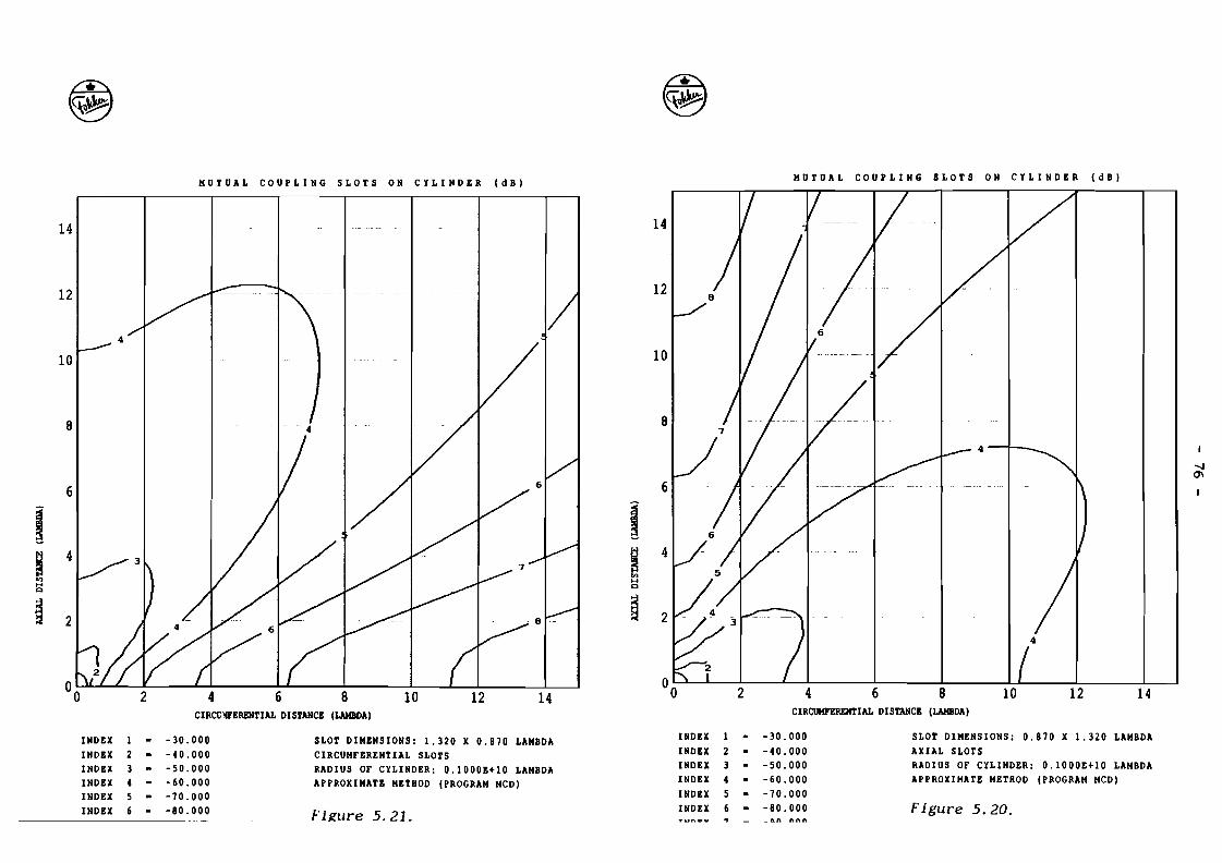
MUTUAL COUPLING SLOTS ON CYLINDER (dB)

14

CIRCl;VERENTIAL DISTANCE (LAMBDA)

MUTUAL COUPLING SLOTS ON CYLINDER (dBt

CIRCUMnRENTIAL DISTANCE (LAMBDA)14

INDEXINDEXINDEXINDEXINDEXINDEX

123456 •

-30.000-40.000-50.000-60.000-10.000-80.000

SLOT DIMENSIONS: 1.320 X 0.810 LAMBDACIRCUMfERENTIAL SLOTSRADIUS Of CYLINDER: 0.1000Et10 LAMBDAAPPROXIMATE METHOD (PROGRAM MCD)

Fli!ure 5.21.

INDEX 1 -30.000 SLOT DIMENSIONS: 0.810 X 1.320 LAMBDAINDEX 2 -40.000 AXIAL SLOTSINDEX 3 -50.000 RADIUS Of CYLINDER: 0.1000Etl0 LAMBDAINDEX 4 -60.000 APPROXIMATE METHOD (PROGRAM MCD)INDEX 5 -10.000INDEX 6 -80.000 Figure 5.20.

_ tU\ 1\1\1\

HUTUAL COUPLING SLOTS ON CYLINDER

~I II

h- nl [ · I IiI II

L" .Ii

I ~I

Ir--.....-.r-_

~

I I

r---

-ZOk,----. -II I I [

-30

1' ........... ! ' D......, I I I:

I I -- --(-.1__ I I I

-401-1-/;--1-----+-1--.....:_~-·-"----T-l

-50

-60

-iO

~<:J

i!:-80...

"":::>0u

:!:::>..il -90

-1002 4 6

DUDJICE (I.AHBDAI

a 10 12 14

AXIAL SLOTS PRIO-OAXIAL SLOTS :0-0CIRC. SLOTS PRIO-OCIRC. SLOTS :0-0

SLOT DIHEBSIOBS: 0.305 X 0.686 LAXBDAR: 119 LAKBDAA"ROXIKATZ HE TROD (PROGRAM HCD)

Figure 5.22.

- 78 -

6 CONCLUSIONS

Comparison of computed and measured values of both the mutual

admittance and the mutual coupling between slot antennas on

ground planes and cylinders, shows that two of the four developed

algori thms provide fast results of sufficient accuracy and are

therefore very useful for engineering applications.

The algorithms for the calculations on a cylinder, an asymptotic

and an approximate method, are very well suited for calculations

on both cylinder and ground plane. The algorithms for the cal­

culations of the mutual coupling between slot antennas on a

ground plane, a Fourier transform method and an asymptotic

method, are less useful, due to respectively a large calculation

time and inadequate representation of the H-plane coupling.

The comparison of coupling calculations for slot antennas on

cylinders with coupling measurements of altimeter horn antennas,

shows that the modeling of the altimeter horn antenna as a slot

antenna is to simple.

However, from this study, conclusions may be drawn concerning the

parameters that influence the coupling between radio altimeter

antennas on aircraft.

- 79 -

REFERENCES

[1] P.A. Beeckman

"Plaatsing van antennes op civiele vliegtuigen"

Report R-AV89.799 Fokker Aircraft B.V., Department EDAV,

group RF, Schiphol-Oost, the Netherlands, November 1989.

[2] Merrell I. Skolnik

"Introduction to Radar Systems"

McGraw-Hill, New York, 1962.

[3] R. Strauch and C. Castinel (TRT)

"Un radioaltimetre de conception avancee"

L'Onde tlectrique, June 1969, vol.49, fasc. 6, p. 615-621.

[4] Aeronautical Radio Inc., Annapolis, Maryland.

ARINC Characteristic 707: Radio Altimeter

§ 2.13 Interchangeability Standards - Antenna Isolation.

[5] J.H. Richmond

"A reaction theorem and its application to antenna impedance

calculations"

IEEE Transactions on antennas and propagation AP-9, Nov.1961,

p.515-520.

[6] R.F. Harrington

"Time-Harmonic Electromagnetic Fields"

McGraw-Hill Book Company, New York 1961.

[7] R.H. Clarke, J. Brown

"Diffraction theory and antennas"

Ellis Horwood Limited, Chichester 1980.

- 80 -

[8] G.V. Borgiotti

"A novel expression for the mutual admittance of planar

radiating elements"

IEEE Transactions on antennas and propagation AP-16, no.3,

May 1968, p.329-333.

[9] G.V. Borgiotti

"Fourier Transform method in aperture antenna problems"

Alta Frequenza, vol.32, Nov. 1966.

[10] M.E.J. Jeuken

"Elektromagnetische antennes I"

Collegediktaat Fakulteit Elektrotechniek,

Technische Universiteit Eindhoven, April 1988.

{11] H. Bremmer

"Electromagnetische golven en antennes"

Collegediktaat Afdeling der Elektrotechniek,

Technische Hogeschool Eindhoven, September 1971.

[12] Z.W. Chang, L.B. Felsen and A. Hessel

"Surface Ray Methods for mutual coupling in conformal arrays

on cylindrical and conical surfaces"

Polytechnic Institute of New York, Final Report (Sept. 1975

- Feb. 1976), prepared under Contract N00123-76-C-0236, July

1976.

[13] S.W. Lee and S. Safavi-Naini

"Asymptotic solution of surface field due to a magnetic

dipole on a cylinder"

Electromagnetics Laboratory Technical Report no. 76-11,

University of Illinois, November 1976.

- 81 -

[14] S.W. Lee and S. Safavi-Naini

"Approximate asymptotic solution of surface field due to a

magnetic dipole on a cylinder

IEEE Transactions on antennas and propagation, vol AP-26 ,

no. 4, July 1978.

[15] S.W. Lee, S. Safavi-Naini and R. Mittra

"Mutual admittance between slots on a cylinder"

Electromagnetics Laboratory Technical Report no. 77-8,

University of Illinois, March 1977.

[16] J. Boersma and S.W. Lee

"Surface field due to a magnetic dipole on a cylinder:

asymptotic expansion of exact solution"

Electromagnetics Laboratory Technical Report no. 78-17,

University of Illinois, December 1978.

[17] S.W. Lee and S. Safavi-Naini

"Simple approximate formula for mutual admittance between

slots on a cylinder"

Electromagnetics Laboratory Technical Report no. 77-13,

University of Illinois, July 1977.

[18] V.A. Fock

"Electromagnetic diffraction and propagation problems"

Pergamon Press, New York, 1965.

[19] J. Boersma

Private comments and amendments on [13]

December 1979.

[20] K.E. Golden and G.E. Stewart

"Self and mutual admittances of rectangular slot antennas in

the presence of an inhomogeneous plasma layer"

IEEE Transactions on antennas and propagation, vol. AP-17,

no. 6, November 1969.

- 82 -

[21] G.E. Stewart and K.E. Golden

"Mutual admittance for axial rectangular slots in a large

conducting cylinder"

IEEE Transactions on antennas and propagation, vol. AP-19,

January, 1971.

[22] K.E. Golden, G.E. Stewart and D.C. Pridmore-Brown

"Approximation Techniques for the mutual admittance of slot

antennas on metallic cones"

IEEE Transactions on antennas and propagation, vol. AP-22,

no. 1, January 1974.

[23] N.W. McLachlan

"Bessel functions for engineers"

At the Clarendon Press, Oxford 1961.

[24] J. R. Wait

"Electromagnetic radiation from cylindrical structures"

Pergamon Press, New York 1959.

[25] P.A. Beeckman

"Resultaten antenne koppelingsmetingen"

Report AV89.385 Fokker Aircraft B.Y., Department EDAY,

group RF, Schiphol-Oost, the Netherlands, June 1989.

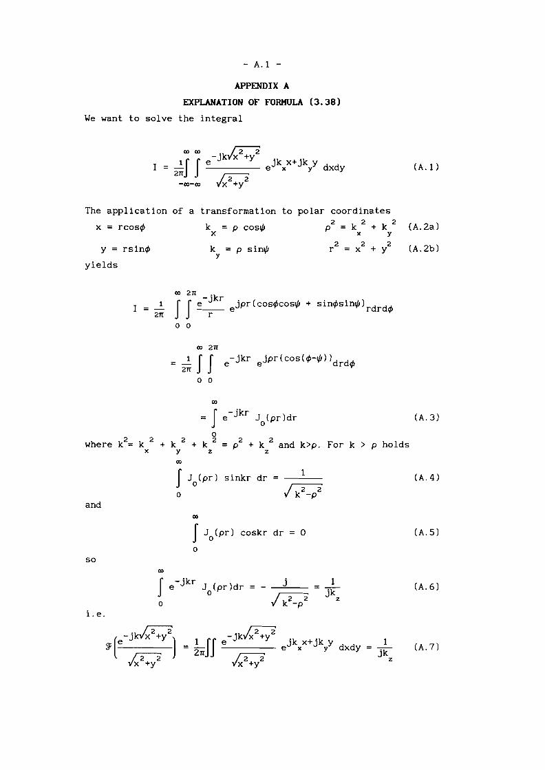
00 00

- A.I -

APPENDIX A

EXPLANATION OF FORMULA (3.38)

We want to solve the integral

·k~II I e-J x +Y jk x+jk Y d dI = 271 --I>--2--i- e x y x Y

-00-00 x +Y

(A.!)

The application of a transformation to

x = rcos¢

Y = rsin¢

yields

k = p cost/Jx

k = p sint/Jy

polar coordinates

p2 = k 2 + k 2x Y

2 2 2r = x + Y

(A.2a)

(A.2b)

I =1

271

00 271 'k-J rI I~ ejpr(cos¢cost/J + sin¢sint/J)rdrd¢

o 0

00 271

= 2~ I I e- jkr ejpr(cos(¢-t/J))drd¢

o 0

00

=I -jkre J (pr)dro(A.3)

o+ k 2 = p2 + k 2 and k>p. For k > P holds

z zwhere k2= k 2 + k 2

x Y00

I0

and

J (pr) sinkr dr =o

1 (A.4)

so

00

I Jo(pr) coskr dr = 0

o

(A.S)

1. e.

00

I e-jkr

Jo(pr)dr =o

j 1= jk

z

(A.6)

~71II1

jkz

(A.?)

- B.l -

APPENDIX B

EXPLANATION OF FORMULA (3.52)

0000 21

12 21

121 1!! k g (k . k) + k g A. (k ,k )( ) P x y' Z 't' X YYd. d = ;-:--:;-;---

12 x Y V V WIl kA B - - z

j(k d +k d ) dk dke xx yy =

x y(B. 1 )

written as

j(k d +k d ) dk dke xx yy =x y

(B.2)

For k2 < k2 + k2 holds k = -jlk I = -j j k2+k2_k2 ' and (3.51)x y z z x y

can be written as

Y (d ,d )12 x Y

j(k d +k d ) dk dke xx yy =

x y

The integrands

and

are symmetrical for both k and k .x y

(B.3)

(B.4)

(B.5)

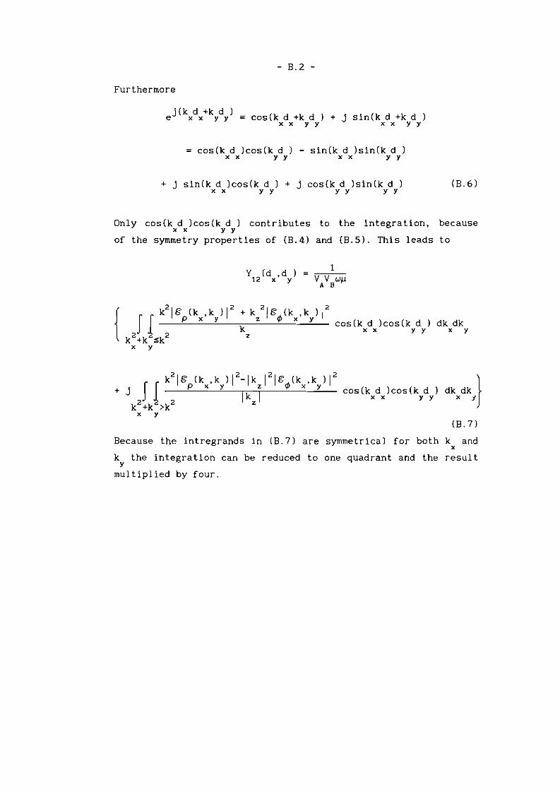
- B.2 -

Furthermore

j(k d +k d )e x x y y = cos(k d +k d ) + j sin(k d +k d )

xx yy xx yy

= cos(k d )cos(k d ) - sln(kd )sin(k d )xx yy xx yy

+ j sin(k d )cos(k d ) + j cos(k d )sin(k d )xx yy yy yy

(B.6)

Only cos(k d )cos(k d ) contributes to the integration, becausex x y y

of the symmetry properties of (B.4) and (B.5). This leads to

Y (d ,d ) =12 x y

1v V W/-l

A B

21 2 2 2

JIk g (k •k ) I -I k 1 Ig rl. (k •k ) 1

+" pxy z 'f'xy

J IkJk2+k >k2 z

x y

cos(k d )cos(k d ) dk dk }xx yy X:l

(B.7)

Because the intregrands in (B.7) are symmetrical for both k andx

k the integration can be reduced to one quadrant and the resulty

multiplied by four.

- C.1 -

APPENDIX C

ZERO'S OF AIRY FUNCTIONS

n It I It' In n

1 2.33811 1. 01879

2 4.08795 3.24820

3 5.52056 4.82010

4 6.78671 6.16331

5 7.94413 7.37218

6 9.02265 8.48849

7 10.04017 9.53545

8 11.00852 11.52766

9 11.93602 11.47506

10 12.82878 12.38479

t = It I - JlI/3 (C.l)en n

t . = It' I e - JlI/3 (C.2)n n

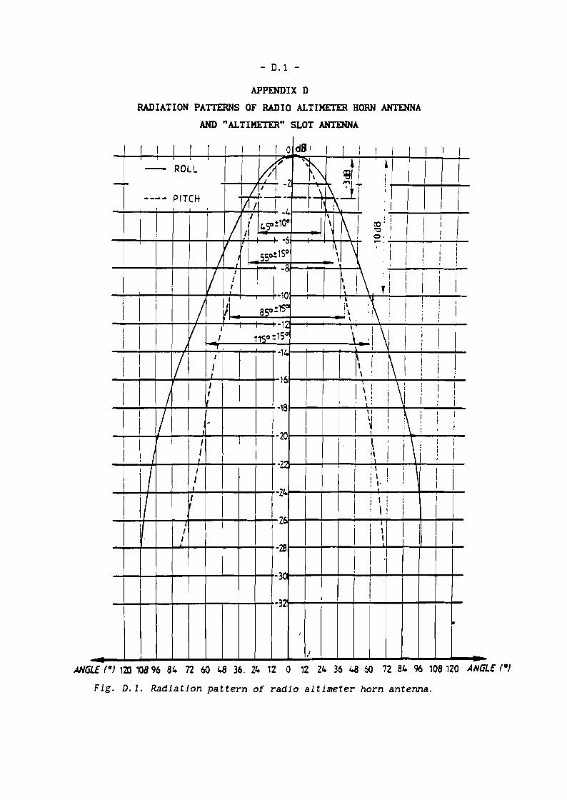
- D.l -

APPENDIX 0

RADIATION PATTERNS OF RADIO ALTIMETER HORN ANTENNA

AND "ALTIMETER" SLOT ANTENNA

, I I I r I I I I '0 d81 , I I I I I I , I

1 - ROLL I ~ ~ '1\ ~t I tI I !,

~I--+----+-~--+P_IT+-CH-+-,~_-i--f-~:/--;'---'--:~~-i-f~ ~~I 'I I I I I

--...--+----i_i--+--i-I----r+/~/l-f+-4_SO......~1: \ ~ i ~ ~ -:-1-+-I--f-I---:...i---;-!_I, I I

IJ i 150 1\ I "I Iii ;/ sso~ I \ . I I : I !

--:-1--:-I--+-I---i---I--+V--I.1+-;-/--+--i-I.:: I \! \ ;I iii r1 I I I / J1 8SO~1~ :\ I ' I ! I ; I I

I

! I I -1.. \ I I :/' I1 / ......./__....:..1'~Slo_:_15~0 \~.! ! I

I / I:' I -l~{j--r-+I~I-+-\.......;...!......\-,,\......i--+i~i--+I-

~i--i---+-I/"'+--+-"""'f-!-+--+-+--+! .::t---;-!---:-1----1'1---:1_\+,\:-1-;-1--+-1_I---.;.!~i:--,,1 , ~I/I......i-~+---t--t----:-1-tI.zol---'-!--+-...l..---__, +I~__:! -+-ll-;'-':_i_!l !I! I I I ~ i i \1 ! I-i----++--+--t-;--~+-+-_t·::2'2'1-.........--i---+--i-"+1.....;...--:-1....1,1+---:,--

i 1,/ Iii \.! I !,--l---J,,-+-+--+--+J.-;--_+-+--r-2lJ-...;--I--+--+......,.-+---.....-~--

I I' I I I I, i ! \! j I--;..--IoIf-+--+---,t--t-;--t-+-+26l--+--+--+-.......-..,..;.--.....;-+-+-~

I I / r i i \ ! I I I--;.~--+-~+-+-~-+--;--+ -2Bt--+-+--+-.........-+-"""'+--+---+--+----I-

I I ! 0'-4-

1

-1--1

-1--1--+--+--+-

1+-+-+-3ot---!--+I!---+--!---i-

I~I---+-+--+-

-+--Io--+---i-I--+-+--+--+--+-321-..~....;--;--+--+----i--+-+-+--+-

I

ANGLE (OJ 120 10896 84 72 60 /J3 36. 24 12 0 12 24 36 /J3 60 12 84 96 108120 ANGLE (oJ

Fig. D.l. Radiation pattern of radio altimeter horn antenna.

- D.2 -

RADIATION PATTERN

o-10

-:lO

-.D

-010

.,.... -~I:D~..., -«lIJI0 -70~

t:Z -aJI:)..;~ -90

-100

-110

-1:20

-13)

O.et1 x 1..J:Z UWBOA

- .-- - --~---~ '" ----~/' "-

/ I"\.I

"'I

-140-90 -1!1 -aJ -ole -.D -15 0 15 030 45 60 75 ~O

RADIATION PATTERNO.f!t1 X 1..J:Z L..AM8CA

A,. """'!IIi~

/'"/ ","r--...

/ " 'l! "-

/ f \. '\./ :l \ \.

/,,: ~

'\.

/ I 1\ \/ 1 \ ~

I-"' II \ -~ l

f '\.t \

t \! ~

t 1-.D

-90 -1!1 -o!lO -45 -.D -15 0 15 030 45 60 75 ~O

0

-2

-4

-6

-a-10.,....

I:D -12~...,IJI -I.a~c -18zI:)

-liS-<~

-:20

-2:t

-24

-28

-2lS

Fig. D.2. Radiation pattern of "altimeter" slot antenna.

- E. 1 -

APPENDIX E

PROGRAMS AND SUBROUTINES

The programs and subroutines are published in a supplement to this

report.