Eindhoven University of Technology MASTER Buffer and ... · model is applied in three case examples...
110
Eindhoven University of Technology MASTER Buffer and inventory management downstream of a cracker a queuing theory approach Puijman, R. Award date: 2011 Disclaimer This document contains a student thesis (bachelor's or master's), as authored by a student at Eindhoven University of Technology. Student theses are made available in the TU/e repository upon obtaining the required degree. The grade received is not published on the document as presented in the repository. The required complexity or quality of research of student theses may vary by program, and the required minimum study period may vary in duration. General rights Copyright and moral rights for the publications made accessible in the public portal are retained by the authors and/or other copyright owners and it is a condition of accessing publications that users recognise and abide by the legal requirements associated with these rights. • Users may download and print one copy of any publication from the public portal for the purpose of private study or research. • You may not further distribute the material or use it for any profit-making activity or commercial gain Take down policy If you believe that this document breaches copyright please contact us providing details, and we will remove access to the work immediately and investigate your claim. Download date: 11. Jul. 2018
Transcript of Eindhoven University of Technology MASTER Buffer and ... · model is applied in three case examples...

Eindhoven University of Technology
MASTER
Buffer and inventory management downstream of a cracker
a queuing theory approach
Puijman, R.
Award date:2011
DisclaimerThis document contains a student thesis (bachelor's or master's), as authored by a student at Eindhoven University of Technology. Studenttheses are made available in the TU/e repository upon obtaining the required degree. The grade received is not published on the documentas presented in the repository. The required complexity or quality of research of student theses may vary by program, and the requiredminimum study period may vary in duration.
General rightsCopyright and moral rights for the publications made accessible in the public portal are retained by the authors and/or other copyright ownersand it is a condition of accessing publications that users recognise and abide by the legal requirements associated with these rights.
• Users may download and print one copy of any publication from the public portal for the purpose of private study or research. • You may not further distribute the material or use it for any profit-making activity or commercial gain
Take down policyIf you believe that this document breaches copyright please contact us providing details, and we will remove access to the work immediatelyand investigate your claim.
Download date: 11. Jul. 2018

Eindhoven, January 2011
--TUE VERSION --
BSc. Industrial Engineering and Management Science (2008)
in partial fulfillment of the requirements for the degree of
Master of Science
in Operations Management and Logistics
Student: Roy Puijman
ID: 0568750
Supervisors: Prof. Dr. Ir. J.C. Fransoo (TU/e, Operations, Planning, Accounting and Control)
Dr. K.H. van Donselaar (TU/e, Operations, Planning, Accounting and Control)
Ir. J. Bisschop (Supply Chain Planning Chemicals, SABIC)
Drs. Ir. R.H.W. van Weerdenburg (Supply Chain Planning Chemicals, SABIC)
Buffer and inventory management
downstream of a cracker:
A queuing theory approach
By:
Roy Puijman

II

III
TUE. School of Industrial Engineering.
Series Master Theses Operations Management and Logistics
Subject headings: Supply chain management, inventory management, buffer inventories, petrochemical industry,
simulation, transient queuing theory

IV

V
Abstract
This study investigates the capacitated inventory control of buffers, and end product and feedstock
inventories in a petrochemical supply chain. We propose a typology to distinguish between different
types of storage and propose a new inventory policy using a transient queuing theory model. We
extend this transient model to a more advanced path simulation model. In the application to three case
studies, both the transient and the simulation model proved to adequately make the complex supply
chain tradeoffs and lead to substantial improvements in the supply chains performance. Furthermore,
the analyses lead to valuable general insights on buffer inventory management.

VI

VII
Management Summary
Petrochemical supply chains often have highly integrated production processes which are decoupled
through storage tanks. Decoupling is necessary because the production processes are characterized
by non-stationary production behavior, among others caused by short term production plan changes
and volatile capacity availability. The tanks however have limited storage capacity, introducing the risk
of blocking and starvation when the tanks are respectively full or empty. Furthermore, there is often
only a limited number of ways to influence the inventory levels in the storages, which is different per
storage type.
This study develops an inventory management policy and corresponding model that can be applied in
controlling capacitated storages in a petrochemical supply chain in a formal, quantitative way. The
model is applied in three case examples in SABIC’s Aromatics supply chain in Teesside, United
Kingdom and was found to lead to a substantial decrease in average inventory levels and to highlight
design improvements on a strategic level to even further improve the supply chain performance. More
specifically, the tool can be applied in the actual redesign projects that are currently executed in
SABIC’s Aromatics supply chain. The model’s general approach allows for easy implementation of the
new inventory policy in other petrochemical supply chains.
Storage typology
Petrochemical supply chains know a number of different types of storage tanks. Current literature
however does not discuss these differences and the differences in the corresponding supply chain
tradeoffs, which is why we propose a formal typology for this.
A distinction can be made between buffers and inventories. Buffers can be further distinguished based
upon their technical capabilities to receive additional purchases, execute additional sales or both.
Furthermore, a buffer’s balancedness is a distinctive factor. In practice, buffers are often unbalanced
(process rate to the buffer (P) does not equal consumption rate from the buffer (C)). Finally, the level
of decision making (strategic, tactical or operational inventory decisions) influences the inventory
control tradeoff. It is of high importance for managers to be aware of the type of storage they want to
control, as different storages require different tradeoffs.
Inventory policy for the unrestricted buffer
We extend the commonly known order-point, order-quantity inventory policy such that it can be applied
to the case of the unrestricted buffer. This (��, ��, �)- inventory policy is shown in the figure on the next
page. The policy proposes to control the buffer through selling or purchasing amount � once the
inventory level respectively exceeds �� or drops below ��.
CP
CP
Relief by additional purchase
Simple buffer Selling buffer
Purchasing buffer Unrestricted buffer
CP C
P
Sales inventory
Feed inventory
CP
Relief by additional sale
InventoriesBuffers
With SalesWithout Sales
Supplier
Additional
sale
Additional
purchase
Customer

VIII
Optimal sales and purchase levels
We design two models that can be used to determine the optimal values of the (��, ��, �)- inventory
policy’s control parameters, the sales level �� and the purchase level ��. Furthermore, the models
propose projected net stock levels for making sales and purchases, which allows for the easy
implementation of the sales and purchase boundaries into SABIC’s mass balances, making the
execution of the formal inventory policy a straightforward exercise.
The first model applies transient queuing theory. The transient model is quick and accurate in finding
the optimal parameters, but lacks the accuracy to determine the total correct Total Relevant Costs
(�) curves. Consequently, we develop a more advanced approach based on random path
simulation. The model determines the optimal sales and purchase levels by minimizing the � and
the corresponding cost curves. The analysis of three case examples creates insights into the typical
shape of the � curve, which is crucial in understanding the inventory tradeoffs. The figures above
show such exemplary cost curves for the observed Benzene case. For the Benzene case, the cost
components are the starvation costs, working capital costs, blocking costs and purchase demurrage
costs.
We conclude that especially the linear part of the � plays a large role in assessing whether or not
the storage capacity is sufficient for optimal inventory management. The smaller the storage, the more
compressed the curve becomes, eventually raising the cost curve when the linear part of the curve has
vanished. Applying the model and observing the cost curves (for multiple parameter settings) appears
to be a valuable tool in setting the optimal decision variables on a tactical level but also in assessing
current supply chain design and highlighting supply chain improvement opportunities.
The general analysis of the unrestricted buffer shows that the optimal inventory policy of unbalanced
buffers only executes the inevitable action (sales for a long buffer, purchase for a short buffer) and
never the opposite. This observation holds only on a tactical level: it is possible to have operational
scenarios that do require the opposite action.
X_max
S_s
X(t)
I(t)
S_p
X_min
LT
Q
Q
TR
C
Purchase level
Purch. Dem.
WC costs
Blocking
Starvation
Total
0
1000
2000
3000
4000
5000
6000
-10000
2100
2900
3700
4500
5300
6100
6900
7700
8500
9300
10100
10900
11700
12500
13300
14100
X_max = 6200
X_max = 8200
X_max = 10200
X_max = 12200
X_max = 14200

IX
Analysis of three case examples: Benzene, Petrinex 6R and Benzene Heartcut
We analyze three case examples with the proposed inventory management model. On a tactical level,
the optimal decision variables and corresponding average inventory levels are determined.
Comparison of the average inventory levels of the new policy to the stock targets of 2010 shows
significant improvements in working capital, as is shown below.
Product Target 2010 Proposed target
WC reduction Winter Summer
Benzene 6,000 4,300 4,300 28%
Petrinex 6R 4,500 3,200 2,600 36%
Benzene Heartcut 15,500 7,600 9,200 46%
Analysis of the � cost curves further shows that currently the combination of the storage capacity
and shipping size for the Petrinex 6R product is insufficient for optimal inventory management. For the
Benzene Heartcut case, the cost curves showed that the tank size is too large in combination with its
current shipment size. Since the � curves do not take into account the costs of additional storage
and the cost benefits of having larger shipping sizes, SABIC is advised to extend the analysis of this
sales and feed inventory to make quick cost improvements.
Inventory management tool
The developed path simulation model is applied into an Excel based decision support tool that enables
a user friendly way of analyzing all possible storage types under all levels of decision making. The tool
results the optimal sales and purchase levels, the projected net stocks for sales and purchases for
easy application into SAP APO, the average inventory level of the optimal policy and the �.
Moreover, the tool allows graphical analysis of the discussed � curves.
Recommendations for SABIC
SABIC is advised to implement the proposed inventory management model and the corresponding
decision support tool in making inventory management decisions on a strategic, tactical and
operational level. Furthermore, SABIC should revise its current inventory performance measurement
system, making use of the quantitative sales and purchase levels and average inventory levels of the
optimal inventory policy. Furthermore, it is advised to involve the Supply Chain Management
department in assessing inventory performance, possibly making the inventory performance a shared
responsibility of the Sales Manager and the Supply and Inventory Manager. Furthermore, it is
recommended to structurally monitor the forecast error performance in order to identify improvement
opportunities and finally to revise the current OTIF customer service policy, as it is found to be useless
in its current form.

X

XI
Preface
Eindhoven, January 23th
, 2011
This report is the result of my Master thesis project which I conducted in partial fulfillment for the
degree of Master in Operations Management and Logistics at Eindhoven University of Technology in
the Netherlands.
I conducted this project from August 2010 to January 2011 for SABIC in Sittard. During the project, I
got to know how much fun it is to put theoretical knowledge into practice in a context as exciting as the
petrochemical industry. This industry, with its large scale, mysterious chemical products and
economical importance offers incredible challenges for every industrial engineer.
During the project, I have had the pleasure to work for and with inspiring people from both SABIC and
Eindhoven University.
From SABIC, I would like to thank Jip Bisschop, the initiator and primary supervisor of the project. Jip
is a young and inspiring guy. His eager to go to the bottom of understanding everything that underlies
‘his’ production processes is unique, inspiring, as well as sometimes a bit scary, as one can be sure
that with Jip, you will never get away with any faulty reasoning. Jip, I hope that we will continue to
collaborate in the future, because there are uncountable things I can learn from you.
Furthermore, I thank Ralph van Weerdenburg as my secondary supervisor. Both in my project, as well
as in my aspirations to find a job within SABIC Chemicals, Ralph always made time for me, guiding me
in project and career management. Finally, I owe thanks to everyone else that made time in her or his
hectic day to provide me with the required information and above all a fun time.
From the university, my thanks go to Jan Fransoo as my mentor and primary supervisor. Discussions
about the project, from detail to strategy, but also about many other topics have always been
downright fun. I can only hope that in personal and professional future, we will stay in touch and
continue to share our passion for Industrial Engineering.
As my second supervisor, I want to thank Karel van Donselaar for his time and critical reviews of my
work.
This project puts an end to my incredibly pleasant years as a student. I will never forget how much fun
the past 6,5 years have been. For this, I thank my friends for their support, the fun and the beers we
shared. Special thanks go to my parents, who supported me in all possible ways throughout my
studies. And Lotte, that I can start the grown-up life with you on my side is probably my greatest
achievement of all. Thank you so much for your patience, love and support.
Roy Puijman

XII

XIII
Table of contents
Abstract V
Management Summary VII
Preface XI
1 Introduction 1
1.1 Project context 1
1.1.1 Product margin pressure from the Middle East 1
1.1.2 Global integration of process industry operations 1
1.2 Project approach 2
2 Buffer and inventory management 3
2.1 Storage typology 3
2.2 Blocking and starvation 3
2.3 Inventories 4
2.4 Buffers 4
2.4.1 Technical tank capabilities 4
2.4.2 Supply and demand dynamics 5
2.4.3 Strategic, tactical or operational focus 5
3 Supply Chain Analysis 7
3.1 Process 7
3.1.1 Production process 7
3.1.2 Demand process 8
3.1.3 Customer service 9
3.1.4 Lead times 9
3.2 Control 10
3.2.1 Strategic control level 11
3.2.2 Tactical control level (S&OP process) 11
3.2.3 Operational control level (WOM) 12
3.2.4 Inventory control process 13
3.3 Organization 14
3.4 Information technology 15
3.4.1 PIMS optimization tool 15
3.4.2 SAP APO 15
3.5 Supply chain performance 15
3.5.1 Production plan forecasts errors 15
3.5.2 Supply chain uncertainties 17

XIV
4 Research approach 18
4.1 Supply chain challenges 18
4.2 Problem definition 19
4.3 Research context 19
4.3.1 Push characteristic of the process industry 19
4.3.2 Capacitated inventory control 19
4.3.3 Non-stationary feedstock supply trough cracker domination 19
4.3.4 Queuing theory methodology 20
4.4 Research questions 20
5 Transient queuing theory model 21
5.1 Buffer and inventory management policy 21
5.2 Steady-state queuing theory models 22
5.3 Transient queuing theory model 22
5.3.1 Transient state probability distribution 23
5.3.2 Transient analysis of the simple buffer 24
5.3.3 Chain effects of blocking and starvation 25
5.3.4 Transient analysis of the unrestricted buffer 26
5.3.5 Drawbacks of the transient analysis 29
6 Simulation model 31
6.1 Random path generation 31
6.2 Inventory related costs and parameters 32
6.2.1 Determining state probabilities 33
6.2.2 Demurrage costs 33
6.2.3 Projected net stock 33
6.3 Total relevant costs 34
6.4 Finding the optimal inventory parameters 35
6.4.1 Decision variables 35
6.4.2 Solution space 36
6.4.3 Time efficiency algorithm 36
7 Results 38
7.1 Buffer management 38
7.1.1 Benzene results 38
7.1.2 Lead time sensitivity analysis 40
7.1.3 Shipment size sensitivity analysis 41
7.1.4 Tank size sensitivity analysis 42

XV
7.2 Sales inventory management 43
7.2.1 Petrinex 6R results 43
7.2.2 Lead time sensitivity analysis 44
7.2.3 Tank size sensitivity analysis 45
7.2.4 Shipment size sensitivity analysis 45
7.3 Feed inventory management 45
7.3.1 Benzene Heartcut results 46
7.3.2 Lead time sensitivity analysis 46
7.3.3 Tank size sensitivity analysis 47
7.3.4 Shipment size sensitivity analysis 47
7.4 Model verification 47
7.4.1 Simple buffer model verification 48
7.4.2 Unrestricted buffer model verification 49
7.4.3 Determining the decision variables with the transient model 50
8 Implementation 51
8.1 Inventory management tool 51
8.2 Workflow implementation 52
8.2.1 Frequency of the analysis 52
8.2.2 Application of the model results in the current SAP APO workflow 52
9 Conclusion 53
9.1 General conclusions 53
9.2 Recommendations for SABIC 54
9.3 Recommendations for future research 55
10 References Error! Bookmark not defined.
11 Abbreviations 59
Appendix A: Supply chain control structure 60
Appendix B: Daily forecast error analysis 61
Appendix C: Daily forecast error distribution fitting 64
Appendix D: Forecast Error Regression Analysis 65
Appendix E: Full problem scheme 70
Appendix F: Inventory model parameters 71
Appendix G: Determining � (Kulkarni, 1998) 72
Appendix H: Transient model for the unrestricted buffer 73

XVI
Appendix I: Cycle length, initial net stock and relevant costs 75
Appendix J: Solution space for path simulation model 77
Appendix K: Time efficiency algorithm 79
Appendix L: Benzene Results – Unbalanced buffer 80
Appendix M: Comparison simulation and algorithm 83
Appendix N: Petrinex 6R Results – Sales inventory 85
Appendix O: Benzene Heartcut Results – Feed inventory 88
Appendix P: Existence of Ss and Sp 91
Appendix Q: Transient vs. Simulation model 92

1
1 Introduction
This study investigates inventory management in the petrochemical industry. Controlling buffers and
inventories, typically having capacitated storage, can be complex. Optimal control of buffers and
inventories involves different tradeoffs depending on a buffers physical capability, a buffers
supply/demand dynamics and the level of decision making.
The Aromatics supply chain of SABIC in Teesside, United Kingdom is considered as a case example.
A steam cracker, the most upstream unit of this supply chain, serves multiple business units and is
operated such that the overall netback of all business units together is maximized. As a result of
smaller volumes and smaller profit margins, the supply to the Aromatics supply chain by the cracker
can be dominated by the other businesses’ supply, which is why this chain has to deal with non-
stationary feedstock supply.
The supply chain under scope has limited storage capacity in between the production units,
introducing the risk of production disruption if tanks are empty or full. Additional complicating factors
are the non-stationary equipment availability, the large shipment sizes and volatile lead times for both
sales and purchases. This study will address the question how to manage such complex supply chains
with capacitated storage by proposing an inventory management policy and a quantitative model of
this policy.
1.1 Project context
1.1.1 Product margin pressure from the Middle East
Tullo (2010) discusses the high competition in the process industry coming from the Middle East,
putting a lot of pressure on the industry elsewhere. Because of the cost advantage in feedstock prices
in the Middle East, Asian and European producers struggle to keep up with the margins that the
Middle East producers can offer. Rooney (2005) discusses the increasing cost advantage of the
Middle East versus Asia: an advantage that increases if the oil price increases. Resulting from the cost
benefit, capacity expansions for ethylene production in the Middle East are large. In 2010 roughly an
additional 4% of the current ethylene production capacity was expected to come available.
Furthermore, Tullo (2010) explains that it was expected that the normal growth in ethylene demand (4
to 5% per year) will not resume until 2011.
Although SABIC is the largest chemical producer in the Middle East, increasing competition is also a
threat for the European assets of SABIC, as they purchase naphtha and other feedstock in the market,
just like all non-Middle East petrochemical producers.
1.1.2 Global integration of process industry operations
Besides the margin pressure coming from high competition, the SABIC case shows that globalization
is increasingly becoming an important practice in the industry. For SABIC, having a global production
network with assets throughout the world, the combination of local feedstock prices, market prices and
capacity constraints introduce the importance of a global alignment of production and demand.
Resulting from the earlier mentioned geographical cost benefits and given production capacity,
production plants at different locations in the world can have significant surplus or shortages of
particular (intermediate) products. An example in the supply chain under scope is the production of
Benzene, an important raw material for many industries, for which there currently is a shortage in the
European market, but a surplus in some other markets.
Practically, this global integration of production networks, referred to by Grossmann (2003) as
Enterprise Wide Optimization (EWO), indicates the importance of really understanding the supply
chain costs and risks of having capacitated storages. These insights are also of high importance in
making investment decisions, such as the investment in storage.

2
1.2 Project approach
The research model by Mitroff et al. (1974), will serve as a backbone of this project. As cited by
Bertrand and Fransoo (2002), the research model proposes four sequential project stages: The
conceptualization phase; Modeling phase; Model solving phase and; Implementation phase, as shown
in Figure 1.
Figure 1.1; Research model by Mitroff et al. (1974)
In the conceptualization phase in Chapter 2 we discuss a conceptual framework to formally capture
the differences between types of storage in a manufacturing flow line. In Chapter 3, we conduct an
analysis of the SABIC Aromatics supply chain, which serves as a case study. The case study’s supply
chain introduces many practical complexities that are dealt with in the buffer management model, such
as capacitated storage and uncertain capacity availability. Furthermore, the case study directly shows
practical examples of the storage typology proposed in Chapter 2.
Chapter 4 describes the research approach by summarizing the primary supply chain challenges,
stating a formal problem definition, research domain and research questions and discusses the study’s
focus on developing a formal, quantitative model to buffer and inventory management.
Chapter 5 and 6 form the study’s modeling phase. In Chapter 5, making use of transient queuing
theory, we develop two simple buffer inventory models that will create more insight into the effect of
having sales and purchase possibilities in buffer. The models introduce the tradeoffs between working
capital costs and the blocking and starvation margin losses. A second, more complex model,
introduces the risks and costs of additional sales, purchases and demurrage. In Chapter 6, extending
the transient models, we develop a simulation model based on random path simulations in order to
overcome the transient model’s drawbacks. Besides the simulation model itself, we develop an
algorithm that enables more efficient simulation analyses. In Chapter 7, we conclude that despite
some drawbacks, the transient models appear to be quite comparable to the simulation models, which
creates high hopes for the applicability of transient models in the future.
The simulation model is verified and put to use in finding the quantitative answers to the research
questions in Chapter 7, the model solving part of the study. Sensitivity analyses are conducted in order
to get a thorough understanding of the previously discussed buffer and inventory management
tradeoffs. The sensitivity analysis to the lead time, shipping size and tank capacity give valuable
insights for managers by quantitatively showing the increase and decrease in supply chain cost. These
insights can be put to use in supply chain redesign decisions. Furthermore, a general analysis is
conducted that shows that for unbalanced buffers, having both a sales and a purchase level on a
tactical level is never really optimal.
Finally, Chapter 7 and 8 form the implementation phase of the study, making recommendations to
implementing the developed model into the case study and discussing the recommendations for future
literature. The application of the decision support tool showed that by applying the new inventory
policy, given the current supply chain design, working capital reductions between 28 an 46% can be
realized.

3
2 Buffer and inventory management
As an introduction to buffer and inventory management, we proposed a typology of storages in
chemical supply chains. Furthermore, the impact of a buffer’s supply and demand dynamics on its
control tradeoffs is discussed. Finally, differences between the inventory management tradeoffs on a
strategic, tactical and operational level are explained. These districting factors lead to different supply
chain tradeoffs, which is why this typology adds to the understanding of buffer and inventory
management in academic literature and in practice.
2.1 Storage typology
A chemical supply chain can incorporate many applications of storage tanks. In order to make
recommendations about controlling these types of storages, a clear typology is required. The proposed
typology is shown in Figure 2.1.
Figure 2.1: Buffer and inventory storage typology
Typical for storages in the production chain of a manufacturing flow line is the fact that material is
primarily put into the storage by means of producing an amount of material per time unit by a producer
(P), and similarly material is taken out of the storage by means of consumption of an amount of
material per time unit by a consumer (C). The producer and the consumer are the supply chain’s own
manufacturing processes and are therefore controlled by the company itself. The Producer (P) and
Consumer (C) should not be confused with respectively external suppliers and customer demand.
These latter concepts can primarily be found in respectively the feed and sales inventories (See Figure
2.1). Buffers can also have external supply and customer demand, but as is discussed later, such
actions solely serve as reliefs in the control of the inventory position in the buffer tank.
2.2 Blocking and starvation
Important concepts to inventory management with capacitated storage are blocking and starvation.
Blocking occurs when a production unit has insufficient inventory space to store produced goods. The
‘head space’ that a unit requires to store produced goods is also referred to as safety ullage, which is
formally defined as the expected amount of storage capacity left right before the quantity of material
sold leaves the tank.
Safety ullage is put in place to avoid blocking in the case that production is more than expected. When
there is insufficient ullage left in the buffer, the unit in front of it might be forced to either reduce its
production speed or shut down completely. This is referred to as respectively partial or complete
blocking (Tan and Gershwin, 2009). Analogously, starvation occurs when a consuming unit
downstream of the buffer has insufficient feed in the buffer to produce according to plan. If the buffer is
CP
CP
Relief by additional purchase
Simple buffer Selling buffer
Purchasing buffer Unrestricted buffer
CP C
P
Sales inventory
Feed inventory
CP
Relief by additional sale
InventoriesBuffers
With SalesWithout Sales
Supplier
Additional
sale
Additional
purchase
Customer

4
running dry, the unit behind the buffer is forced to decrease production or to shut down completely.
This is referred to as partial or full starvation (Tan and Gershwin, 2009).
2.3 Sales and feed inventories
Inventories either hold end products (sales inventory) put in place to serve the customers, or external
feedstock (feed inventory) put in place to store feedstock before it is consumed in the manufacturing
process. Sales inventories run the risk of blocking their predecessor, while feed inventories run the risk
of starving their successor. Furthermore, sales inventories have to make sure there is sufficient supply
to meet customer demand. Likewise, feed inventories have to make sure there is sufficient storage
capacity left to be able to put in the ordered replenishments into the tank upon arrival (ullage).
In a sales inventory, which is only connected to a Producer, material flows into the storage, but
material can only flow out of the storage by executing a sale. For this reason, sales net stock levels
never decrease over time can, unless a sale is executed. The opposite is true for the feed stock point.
2.4 Buffers
According to Jensen et al. (1991), a buffer’s main purpose is to protect the supply chain against stage
failures at the factory upstream and downstream of the buffer to avoid blocking and starvation as much
as possible. Opposed to sales or feed inventories, buffers are always connected to two manufacturing
processes (P and C). Buffers are therefore a decoupling point in the manufacturing process. We
describe three reasons for decoupling:
1. Asynchronous production of different units
2. Non-stationary production capacity availability (equipment uptime)
3. Intermediate products can be sold
The first reason comes from the fact that asynchronous production of different units (factories) without
decoupling would force all units to work according to the pace of the bottleneck in the production
chain. If would be no possibility to store intermediate products, all production steps would be fully
dependent on each other.
The second reason to decouple comes from the fact that production assets typically have volatile
availability. Production units might (partly) fail, resulting in a decrease in production capacity. Inventory
can be put in place in the buffers to be able to secure the supply to the consumer for a period of time,
or to secure the storage for a buffer’s producer.
The third reason to decouple comes from the fact that depending on the market price of the
intermediate product, it is possible that one would make more profit selling the intermediate product
instead of transforming it into end product, even though this could mean that the downstream unit
works under its maximal utilization. Furthermore, it is also possible that because of capacity decreases
(e.g. shutdowns), keeping material in the buffer for consumption is unnecessary and selling is a better
idea.
2.4.1 Technical tank capabilities
Buffers exits in many types. We differentiate between the types of buffers based upon their technical
capabilities, supply and demand dynamics and the focus of the inventory control. The distinction
between types of buffers is based on the tank’s technical capabilities like valves and pumps. These
capabilities are necessary to make it physically possible to take additional material out or put additional
material in. Consequently, one can make a distinction between buffers that have the freedom to sell
additional material from the buffer, purchase additional material and put it into the buffer, or both.
Additional purchases and sales should be viewed at as additional degrees of freedom to controlling the
buffer level without influencing production and consumption. This property creates the distinction
between the ‘simple buffer’, ‘selling buffer’, ‘purchasing buffer’ and ‘unrestricted buffer’ (Figure 2.1).

5
2.4.2 Supply and demand dynamics
A second distinction between buffers comes from its supply and demand dynamics. There are three
means of controlling a buffer’s net stock:
1. Adjust the production and consumption rates
2. Adjusting the quantities and the timing of existing sales or purchases.
3. Plan new sales and purchases.
For the ‘simple buffer’, additional sales and purchases are physically impossible because it lacks the
technical capabilities. One can only control the buffer through adjusting the producer and consumer’s
rates at which they make material flow into or out of the tank. Consequently, on the long run, it is
unlikely that a planner would choose the production and consumption rate to be very different, as this
would guarantee a buffer going into a state of blocking or starvation. A planner will therefore balance
production and consumption, trying to keep the buffer on constant level. In this case, the buffer is
referred to as a ‘balanced buffer’.
For the selling, purchasing and unrestricted buffer however, the net stock in the buffer can be
influenced by respectively additional sales, purchases or both. Consequently, it is not by definition
necessary to balance the buffer’s production and consumption rate. A distinction can be made
between the balanced and unbalanced buffers, based upon the buffer’s supply and demand dynamics.
In practice, there are three different supply and demand dynamics, following from the average amount
produced and consumed by respectively P and C (�� and � ):
• �� > � - Excess - “Being long”
• �� < � - Shortage - “Being short”
• �� = � - Balance - “Being balanced”
Long and short buffers are defined as unbalanced buffers. �� and � refer to the long run, planned
production and consumption rates per time unit. Consequently, it depends on the planned difference
between production and consumption whether or not a buffer is referred to as balanced or unbalanced.
For the selling, purchasing and unrestricted buffers, the supply and demand dynamic is a result from
the optimal production plan and manufacturing constraints. For example, if the maximal production of
Aromatics feedstock by the cracker is higher than the capacity of the first Aromatics production unit,
stock will inevitably build up. However, as the amount produced follows from the optimized production
plan and the capacity constraints cannot be adapted, balanced operation of this buffer is not optimal
and therefore unwanted. The fact that in this case the buffer is “long” is assumed as a given and
simply has to be dealt with.
Observe that sales, purchase and unrestricted buffers can be both balanced and unbalanced, and that
sales and feed inventories are by definition unbalanced. The distinction between the balanced and the
unbalanced is relevant because of two general observations, which will play a role in the stock
management model.
1. Unbalanced buffers have no fixed optimal inventory position as the net stock is never
expected to be constant;
2. For unbalanced buffers, in the case of being short, purchases are inevitable. Likewise, in the
case of being long, sales are inevitable.
2.4.3 Strategic, tactical or operational focus
On top of the technical capabilities and a buffer’s (un)balance, buffer and inventory management
decisions are subject to the level of focus, which means that the tradeoffs might differ for strategic,
tactical and operational decisions. A related distinction in focus is discussed by Govil and Fu (1999),
who differentiate between a Design, Planning and Control focus to be made by queuing theory
models.

6
Strategic buffer focus
As in queuing theory, design (what we call strategic) decisions are decisions that are related to finding
the optimal design of the supply chain, given a particular operating constraint (Govil and Fu, 1999).
Exemplary strategically focused inventory management decisions are:
• Finding the most economic sizes of the buffer tanks
• Finding the most economic shipment sizes for sales and replenishments
• Negotiating the required lead time for vessels with logistic service providers
Strategic decisions often involve investments (e.g. purchasing or renting additional storage) that have
to be returned within a specific period. Most often, these decisions have a horizon of a year or more.
As an example, because of trading possibilities, management might consider building or renting
additional storage tanks for a particular product. Given the same supply and demand behavior, larger
storage tanks might lead to a decrease in blocking and starvation risk. Furthermore, a larger tank
might introduce the possibility to work with larger shipment sizes, leading to lower costs as a result of
higher economies of scale in logistical costs. That quantifying the benefits of changes in the supply
chain design requires a proper quantitative model to support the business case of the investment.
Tactical buffer focus
Planning models (which have a tactical focus) determine the optimal operating policies so as to
optimize the performance measures of the system (Govil and Fu, 1999). Consequently, a tactical
buffer and inventory management model aims at finding an optimal inventory policy and the optimal
values of the decision parameters for the longer term, averaged situation. These parameters would
lead to the optimal way of controlling the inventories given the average behavior of the system.
Tactical focused decisions would typically be applied as frequently as the average supply chain
dynamics do not change significantly. E.g., in the case of seasonality, tactical buffer decisions may be
made for each season.
Having a tactical focus means that some inventory management actions are inevitable (e.g. sales for a
long buffer). For such inevitable actions, costs should not always be treated as relevant costs.
Typically, tactical decisions do not incorporate occurrences as temporary shutdowns due to planned
maintenance or other capacity exceptional production plan disruptions, as this is information that is
assumed to be unknown on the tactical level.
Operational buffer focus
Operational inventory decisions focus on a specific situation that is expected to happen in the future.
This implies that these decisions have larger level of detail than tactical decisions and more
information is known. For example, the situation in which is known that from 10 to 15 days from now,
consumption is going to be zero as a result of planned maintenance involves an operationally focused
decision whether or not to sell additional material from the buffer. For such decisions, the time horizon
is typically quite short (2 months to half a year).
When making operationally focused inventory related decisions, decisions should always be seen as
an investment that has to return its value. For example, in a case of a sale, the logistical costs of this
sale should be returned by for example lower inventory related costs. Such costs are seen as an
investment because operational decisions are, if they deviate from the tactical decisions, exceptions to
the regular way of working.
The developed inventory management model in Chapter 6 is suitable to make decisions for all types of
buffers, balanced and unbalanced on all possible levels of focus. Throughout the rest of the study, this
proposed buffer typology is applied.

7
3 Supply Chain Analysis
In this chapter, the case study’s supply chain is described. The concepts and models developed are
applied to this case example. Following the framework of Bemelmans (1986), the supply chain is
analyzed, in order to create understanding of the practical complexities of buffer and inventory
management in a petrochemical supply chain.
3.1 Process
3.1.1 Production process
Figure 3.1 shows the production process of SABIC’s production plant in Teesside, United Kingdom, on
a high level. The steam cracker, which is the most upstream unit in the production process, transforms
a combination of three possible types of feedstock into roughly 4 streams of products that are either
sold or transformed further into end products.
Figure 3.1: SABIC’s Teesside production process on a high level
The cracker makes use of steam to break up the molecules in the feedstock and separate them. It has
multiple furnaces, which all can be set to a specific feedstock and operated differently. Depending on
the feedstock prices, feedstock availability, operating constraints, and the prices and expected
volumes of end products, an optimal overall production plan of the cracker is made. The reader is
referred to Puijman (2010) to get more insight into cracking operations and cracker optimization
models.
Although the cracker serves three different business units, it is controlled centrally by the supply chain
management (SCM) department. For certain prices of feedstock and products, optimization might point
out that the production of for example Olefins is most profitable and SABIC should operate the
feedstock that leads to the maximal production of Olefins. This means that C4s and Aromatics will
have less feedstock for their downstream productions. In practice, this occurs quite frequently and is
referred to as the domination of the cracker operation by Olefins.
Although the cracker always cracks a minimum number of its furnaces on naphtha (a broad definition
of a product mixture that is produced when refining crude oil) it also has the possibility to crack
Propane (C3) and Butane (C4). Containing less heavy carbohydrates, which are important to the
feedstock to Aromatics, operating cracking furnaces on gas instead of naphtha has a linear decreasing
effect on the amount of Aromatics feedstock. This is a complexity that the downstream Aromatics
supply chain has to deal with.
Downstream of the cracker is the Aromatics supply chain that transforms the feed stream of C5+ that
comes out of the cracker into a number of intermediates and end products. A graphical representation

8
of this Aromatics supply chain is given in Figure 3.2, which gives a schematic overview of the supply
chain and indicates the boundaries of the project scope.
The production units (squares) and the storage tanks (triangles) are generally labeled instead of using
the real product and facility names. Observe that the coloring in the buffer and inventories in Figure 3.2
refers to the typology of Figure 2.1. Part of the complexity of managing the storage tanks in this supply
chain comes from the capacitated storage: Tanks have a minimum inventory position (����) and a
maximum inventory position (����). A tank’s minimum level is also referred to as the tank heel, the
amount of material that cannot be taken out of the tank in normal operations.
Figure 3.2: Aromatics Supply Chain Teesside
3.1.2 Demand process
A distinction is made between internal demand and external demand. Internal demand comes from
within the organization of SABIC. The most important internal customer for the supply chain under
scope is the Polymers production facility on the SABIC UK site, which is the largest and most
important customer of Olefins. As such, Polymers strongly influence the demand for Olefins and
consequently influence the optimal operation of the cracker. Besides internal demand, three types of
external demand can occur:
1. Spot Sales 2. Contract Sales 3. Swap
Spot sales opportunities result from excess production when all contractual obligations are fulfilled.
Production excesses are anticipated and spot sales are arranged by the Sales Manager. Besides spot
sales, also contractual sales exist, in which most often yearly agreements with customers are made
against a fixed contract price. According to the Sales Managers, there is a noticeable trend that
customers increasingly prefer spot sales over contractual sales, to remain flexible. Finally, products
can also be sold through a swap. A swap is a product trade with another company. In a swap, SABIC
transports products to a competitor in exchange for a shipment of product elsewhere at a different
moment.

9
Specific for the petrochemical industry for commodity products is that there is close to always demand.
This means that or products can always be sold and product obsolescence is irrelevant. Furthermore,
for some products there is a strong focus on contractual sales. This explains that the industry tends to
focus more on capacity utilization maximization instead of on demand forecasting (the industry is
supply driven, rather than demand driven). However, sales in a saturated market might have an effect
on the prices of the product. Furthermore, a spot sale that has to take place within a certain time
window might make SABIC appear urged to sell product, what might have a negative effect on the
price. The assumption is made that for the products under consideration there are always possibilities
to sell the product, which is why demand uncertainty is left out of scope of the project.
3.1.3 Customer service
Customer service at SABIC, but more general in the petrochemical industry, raises an interesting
discussion about customer service measures. Customers, both for spot and contractual sales, tend to
be very flexible. Furthermore, they are believed to be insensitive for the immediate availability of
material when they would like to buy SABIC material. From an inventory management perspective, this
means that material is not kept on stock to cover demand uncertainty. The material in storage is either
a result of the preferred production workflow (e.g. shipment sizes) or put in place for guaranteeing an
optimal production process. It is observed that in the supply chain under scope, traditional customer
service measures as fill rate (see Silver et al., 1998) are not focused on or measured.
Theoretically, SABIC has a customer service philosophy called On-Time, In-Full (OTIF). OTIF
represents the ideal situation that both sales and purchases are executed in the quantity and at the
time that was agreed upon. Interestingly, OTIF is not measured or taken into account in inventory
management decisions. It is an interesting question whether or not this should be done, as it is not
unthinkable that a better OTIF performance will lead to a large customer satisfaction. Currently, OTIF
is not measured or steered upon and the general idea exists that utilizing the customer and supplier
flexibility does not harm the customer’s or supplier’s satisfaction about SABIC.
3.1.4 Lead times
The most popular transportation modality in the supply chain under scope is the deep sea vessel. This
modality can have limited availability, fixed and large shipping sizes and planning uncertainty. This
leads to possibly long and volatile lead times of sales and purchase shipments. The lead time plays a
large role in developing an inventory management policy as it represents the effectuation time of a
purchase or sales decision. We make a distinction between sales and purchase lead times. A lead
time is defined as the time that it takes for a Sales Manager to, in the case of either a sale or a
purchase, get the material literally out of or into the storage. That means that the definition of the lead
time is best represented as in Figure 3.3, which is specific for the case of a sale.
Figure 3.3: Graphical representation of sales lead time
The lead time and its volatility depend on the type of product one wants to transport with the vessel, as
vessels are often product specific. In most cases, vessels can be arranged quite reliably within 10
days as a result of contractual agreements. In their tight schedule however, vessels face uncertainties
as congestion in ports, cargo unavailability and travelling time due to changing weather conditions.
Find customer
Find vessel
Sailing
Waiting
Loading
Signal the need
for a sale
Customer found,
deal made
Vessel arranged
and nominatedArrival in UK
NOR:
Start loading
Vessel loaded/
Product out of
the tank
Lead time

10
This is why logistics service providers work with so-called laycans and demurrage costs, concepts
which are clarified in Figure 3.4. The laycan concept introduces the non deterministic nature of the
lead times. However, although there is volatility in the lead time, we state that this lead time volatility is
not so bad, compared to the volatility that shipments coming from other continents have (see
Langendoen, 2009). Observe that in buffer inventory management, the relevant lead time volatility is
the extent to which a shipment can be earlier or later than the initially agreed (un) loading moment.
Demurrage costs are costs that have to be paid if vessels have to wait to load or unload longer than 20
hours after their Notification of Readiness (NOR). On average, demurrage costs are €10.000,- per
vessel, per day. Consequently, incorrect inventory management can cause demurrage costs if:
1. The amount of product to be shipped for a sale in not available
2. There is insufficient storage room in the tank to discharge the amount purchased
Figure 3.4: Graphical representation of demurrage
As no data on lead times is available, lead time estimations are made through interviews with Sales
Managers, shown in Table 3.1. These estimations will are used in the inventory model, which means
that lead time volatility effects is not taken into account. However, recommendations are made in how
to deal with the lead time volatility in applying the developed inventory models. We conclude
deterministic lead times seem to be an acceptable assumption as volatility is not extremely large and
the extend of the shipping delays is limited by the fact that, if a vessel requests an extreme extension
of the laycan, SABIC can most often arrange another shipment within a number of days.
Product Market liquidity Lead time (days)
Buffer 1 Tight 30
Buffer 2 Tight 20
Buffer 3 Liquid 10
Product 1 Tight 30
Product 2 Liquid 10
Product 3 Liquid 10
Product 4 Tight 30
Feedstock 1 Tight 30
Table 3.1: Lead time estimations
3.2 Control
Figure 3.5 is a graphical representation of SABIC’s supply chain control structure. The control
structure is discussed on a strategic, tactical, operational and execution level. A more extensive
representation of the control process is shown in Appendix A.

11
Figure 3.5: Aromatics control structure
3.2.1 Strategic control level
On a strategic level, there is the budgeting cycle, of which an important element is the setting of
inventory targets. Currently, inventory targets are set on experience and hindsight, and agreed upon
by the business management. Experience and hindsight however are no guarantee that the right
inventory targets are set, but are inevitable because of the absence of a formal inventory model.
Consequently, the set inventory targets are not always believed to be correct. A striking observation
regarding the inventory targets is that they are monitored by the Control department at the end of each
month, based upon the inventory positions at the end of that particular month. Such one moment
observations however may lead to a false picture of the inventory behavior and might encourage non
optimal inventory decisions by the people that are held accountable for following the inventory
positions.
Besides the budget cycle, the strategic level involves investment decisions of which examples have
been discussed in Chapter 2. Currently, investment business cases are not always adequately
supported by quantitative and risk analyses because of the absence of inventory models. Furthermore,
the actors involved in making the decisions not always fully comprehend all sides of the supply chain
effects of certain decisions.
3.2.2 Tactical control level (S&OP process)
The control process on a tactical level is referred to as the monthly Sales and Operations Planning
(S&OP) process. Sales and Operations Planning is a monthly planning cycle with a meeting at the end
of each month, in which the optimized production plans for the upcoming two months are being
presented, discussed and approved. The primary planning output is:
• Cracker furnace planning (feedstock type and operating parameters)
• Forecast of production and consumption rates on daily basis for the upcoming month
• Planning of existing (contractual or already made spot) sales and purchases
• Insight in the profit margins of feedstock types and different products
The proposed production planning is based upon an optimization made by the Supply and Inventory
Manager (SIM) (see Appendix A). The S&OP for the UK site generates production and consumption
forecasts on a daily basis for the upcoming month. The furnace planning is made for the upcoming
three months, but the rest of the plan has an 18 month horizon.
Because the cracker production plan affects Olefins, C4s and Aromatics production, the S&OP plan
consists of three parts. The meeting is prepared and chaired by SCM and the attended by the
concerned business managers, manufacturing, site logistics and control. Interestingly, in the current
situation, the S&OP meeting is not always attended by the concerned Sales Managers (SM). It is
argued that this comes from the fact that the sales timing is only discussed on a tactical level in the
S&OP plan. This absence however is still considered quite remarkable because poor sales timing can
bring the production process in danger and can lead to high inventory positions and is therefore an
important subject that could be challenged in the S&OP, in the Sales Manager’s presence.

12
In the current situation, performance of the SM is judged by the business management. However, this
is done in the absence of SCM, which is observed to have the best understanding of supply chain
effects and therefore as the right actor to adequately assess the sales and purchase timing
performance of the SM. We conclude that accountability for inventory positions and the possible
effects of wrong inventory decisions is not indisputably clear.
As an input for making the S&OP plan, the SIM makes use of four types of (forecasted) information:
1. Demand information
2. Supply information
3. Price information
4. Manufacturing constraints
Demand information can concern either internal or external demand. Having the right demand
information is crucial. For example, if for some reason there is no Olefins demand from Polymers, this
might have consequences for the operation of the cracker and therefore for the other businesses as
well. Demand information is supplied by the previous tactical S&OP plan, the Polymers S&OP plan
and the respective sales and business managers.
Supply information is primarily related to the availability of particular feedstock types. Since the
Feedstock business unit also has to deal with non-stationary supply from feedstock suppliers (e.g.
long, uncertain delivery lead times), the availability of feedstock can differ widely. Furthermore, the
feedstock traders are looking in the market for economical feedstock deals, which might lead to ad hoc
feedstock purchase decisions.
Price forecasts are the most important inputs for the PIMS optimization. The main decisions for the
cracker operation are the number of cracking furnaces to be set to which feedstock. From practice it is
known that although the price forecasts are crucial to make these decisions, the forecasts are difficult
to make as they show very close relations to the crude oil market price, which generally acknowledged
by practitioners to be highly unpredictable.
Furthermore, there are manufacturing and logistical constraints to be taken into account in the S&OP
plan. Aspects like planned maintenance might restrict the process capacity in the chain, creating
bottlenecks that have to be taken into account. Furthermore, because of the interdependency of
different production units in the manufacturing flow line, manufacturing constraints throughout the
entire production site might create bottlenecks that have to be taken into account to avoid upstream
effects of blocking and starvation.
The tactical process as shown in Appendix A is the process as it was designed. In the current
situation, this process is followed for most of the time, although the sequence of the process steps can
have a somewhat organic behavior. This however does not necessarily lead to explicit problems, but
does create a somewhat unsustainable workflow, as it strongly depends on good relationships
amongst and implicit knowledge of the actors.
Finally it is observed that sometimes somewhat simplistic calculations are used in for example sales
timing decisions. For example, the blocking risk of a sales decision might be determined through
deterministic calculations with average production rates, disregarding risk of blocking induced by non
stationary production behavior. Although this can be explained by the absence of a formal inventory
model, it also indicates a lack of understanding and insights in the supply chain related risk and costs.
3.2.3 Operational control level (WOM)
The Weekly Optimization Meeting is the short term, weekly equivalent of the S&OP and occurs at the
beginning of every week. As for the S&OP, demand, supply, prices and manufacturing constraints are
forecasted and used as input for the optimization of the weekly optimized production planning, which is
agreed upon in the Weekly Optimization Meeting (WOM). The WOM plan allows for only minor
changes in the S&OP production plans. The WOM also takes input from the Product Flow Meeting
(PFM), in which weekly operational issues are being discussed between operations and SCM.

13
In practice, it does occur that the S&OP production planning is adjusted in the WOM as a result of
renewed insights in for example product prices. Currently, within the organization, it is disputed
whether or not such changes are improvements in the end. Short term changes might lead to more
profit, but also create turbulence in the process if the short-horizon price if the forecast errors of the
short term forecasts turn out to be still large.
Figure 3.6: Organizational roles in Supply Chain Control
In Figure 3.6 the actors in the control process can be seen. The figure represents the formal
collaborations and responsibilities in the control process. However, on the operational and execution
control levels, the control process also might display some dependency on informal information
sharing and strong dependency on the knowledge of individual actors.
In the current situation it is observed that although formally it is known what responsibility belongs to
which actor, (e.g. production planning belongs to the SIM), practice shows that some play a large role
in other actors’ responsibilities as well. For example, in the planning of sales and purchases, the SIM
plays a major role in the decisions whether or not additional sales or purchases have to be made. This
happens because of the observation that the true supply chain knowledge, the understanding of all
sides of purchase and sales planning decisions, lies currently with the SIM. This is not necessarily a
problem but raises the question if the ones responsible for sales and purchase decisions and inventory
positions are the ones that should be.
3.2.4 Inventory control process
On the execution level, there are six ways to physically influence the amount of material that flows into
(or flows out of) a buffer. These control mechanisms are schematically shown in the Figure 3.5.
Obviously, not all of these mechanisms can be applied to all sorts of buffers and to sales and feed
inventories, but the mechanisms are presented generally.
Adjust inflow to storage tank Adjust outflow from storage tank
Adjust production rate Adjust consumption rates
Adjust existing sales
1. Change purchase quantity
2. Change purchase timing
Adjust planned sales
1. Change sales quantity
2. Change sales timing
Make a new purchase Make a new sale
Table 3.2: Inventory control mechanisms of a buffer
Firstly, there is the possibility to increase or decrease production to a storage or consumption from a
storage. This is referred to as adjusting the production planning, decided upon in the S&OP or WOM.
Changing these optimal plans is by definition expected to negatively influence the performance of the
supply chain. Secondly, the inflow and outflow of material can be influenced by adjusting already
planned purchases and/or sales. As this is often done on an operational level, these actions are often
executed by the Customer Service Officers. Practically, this can be done in two ways:
1. Change the agreed purchase (or sales) quantities
2. Change the timing of purchase (or sales) execution
14
Keeping in mind SABIC’s OTIF philosophy, is it questionable if this second control mechanism can be
rightfully applied. This is a very interesting discussion, since it is not agreed upon by everyone in the
organization that this control mechanism is harmful for customer satisfaction. The ‘requests for
flexibility’ are typical for the industry and in some people’s opinion “common practice”. As said before,
the question is whether or not this control mechanism is preferred, not preferred or only an emergency
measure. For the project, it is decided that customer/ supplier flexibility is not preferable and will
therefore be left out of scope.
The third mechanism in influencing the material in a tank is by planning new purchases or sales.
Although it should be kept in mind that bringing in or taking out additional material might be costly
(primarily because of logistical costs), this control mechanism does not harm the optimal production
plans or requires customer or supplier flexibility. Obviously depending on the type of buffer, the
question is at which inventory positions additional sales or purchases should be made. These levels
are referred to as Sales and Purchase TBA (To-Be-Arranged) level, which are currently determined on
gut feeling and experience.
3.3 Organization
The Saudi Basics Industries Corporation (SABIC) is one of the world’s leading manufacturers of
commodity and specialty chemicals, polymers, fertilizers and metals. SABIC was founded in 1976 in
Saudi Arabia. SABIC started as the first company to make use of natural gas, the by-product of oil
extraction, for the production of petrochemical products like polymers. The company grew towards
being the largest and most profitable non-oil company in the Middle East and one of the world’s five
largest petrochemical manufacturers. SABIC is a public company based in Riyadh. 70% of its shares
are held by the Saudi government and the remaining 30% are held by private investors.
SABIC has around 33,000 employees, serving customers in more than 100 countries. In 2009,
SABIC’s total revenue was around 27 billion USD, leading to a net income of 2 billion USD. This result
was achieved with a total production of 58 billion metric tons of products, of which 60% is accounted
for by chemicals products. Chemical products are made by the Strategic Business Unit (SBU)
Chemicals. Other SBUs are shown in Figure 3.7.
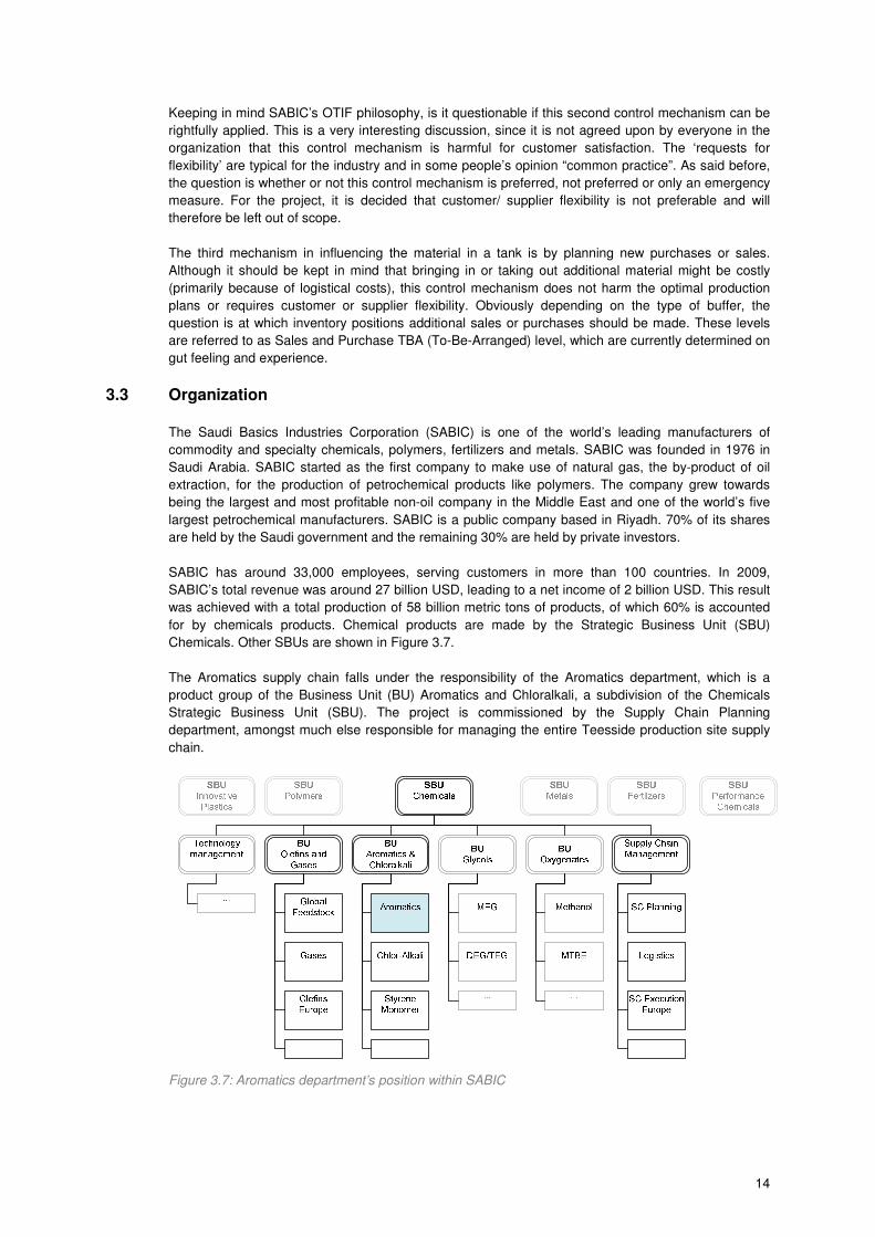
The Aromatics supply chain falls under the responsibility of the Aromatics department, which is a
product group of the Business Unit (BU) Aromatics and Chloralkali, a subdivision of the Chemicals
Strategic Business Unit (SBU). The project is commissioned by the Supply Chain Planning
department, amongst much else responsible for managing the entire Teesside production site supply
chain.
Figure 3.7: Aromatics department’s position within SABIC

15
The primary actors for the project are discussed in Section 3.2. However, it is primarily the SIM that
will use and apply the developed inventory management model in quantitatively supporting the setting
of sales and purchase levels. Although the model could also be used by the MPS, SM and CSO, these
actors will primarily execute policy and therefore play a secondary role.
3.4 Information technology
3.4.1 PIMS optimization tool
PIMS is an optimization tool for cracker operation planning and is primarily used in the S&OP and
WOM process. It incorporates a complex Mixed Integer Nonlinear Programming model of the cracker
that maximizes the overall profitability of the cracker and downstream operations. The reader is
referred to Puijman (2010) for more information about cracker optimization models. As primary tool in
the S&OP process, PIMS takes fixed inputs of price forecasts and requires demand, supply and
manufacturing constraints as input as well.
The PIMS optimization also expresses the cracking-value, expressing the profit a volume of feedstock
yields as a percentage of a base line Naphtha price. This cracking value can be used by the feedstock
traders in finding interesting feedstock deals, as they will aim at maximizing the spread between the
cracking value and the feedstock price. PIMS expresses the cracking-value for each additional
furnace, so that for each furnace the most profitable feedstock can be selected. Currently, the PIMS
tool has only recently become operational for the Teesside production site.
3.4.2 SAP APO
The tactical and operational plans of production, sales and purchases are managed by the Advanced
Planning Optimization (APO) tool, an SAP software package. This software package has been
developed and rolled out two years ago in a project called SUNRISE.
APO incorporates tactical and operational plan books for all products, fed by all actors in Figure 3.6.
The plan book balances out end stocks on a daily basis for the upcoming two months. For the rest of
the months, it does this on a monthly aggregated basis. Plan books are used for monitoring if and
when additional sales and purchases should be executed (Sales and Purchase TBA levels). In
developing a mathematically and model based approach to inventory management, the plan book way
of working in the current workflow is taken into account, in order to enable a smooth implementation of
the new inventory management policy.
In most inventory policies (e.g. De Kok, 2005), the inventory position is used to base purchase
decisions upon. The inventory position is the physical net stock, corrected for additional purchases and
sales that are made but are still to be executed in the future. However, the plan-book way of working
implies that instead of deciding upon making a sale or purchase when the inventory position as a
certain level, sales and purchase decisions have to be executed when the expected physical stock
level has a certain value. An ideal Sales or Purchase TBA level would indicate the execution of a sale
or purchase, rather than the moment at which the sale or purchase has to be made. The ideal picture
of a TBA level is taken into account in developing the inventory policy.
3.5 Supply chain performance
3.5.1 Production plan forecasts errors
As discussed in Section 3.3.2, the S&OP plan makes predictions of the daily production rates of the
upcoming month. In this section, forecast errors of these predictions are discussed. These forecast
errors are defined as the deviation of the realization of the production plan from the planned production
plan.In the hypothetical situation that the S&OP plans predictions have no volatility, the supply chain
would be fully predictable. In that case, the development of the material in a (buffer) inventory would
be predictable and blocking and starvation would never occur. Unfortunately, fully predictable

16
production rates are an ideology. It is exactly the volatility in the production (and the sales and
purchase) plan that the supply chain has to be protected against. Observe that in general, a better
prediction of the production plan would lead to less volatility in the supply chain, making managing the
chain less complicated and costly.
We distinct between three global causes of forecast errors in the production plan:
1. Planning model errors
2. Forced plan changes
3. Conscious plan changes
The first cause refers to the fact that however the model might predict for example a certain quantity of
Aromatics feedstock, given a particular furnace setting, feedstock and operating mode, this prediction
is based on estimation and the realization is likely to be different, even though if the parameters used
in the model appear to be correct. Consequently, this cause of forecast errors can only be changed by
improving the planning models used.
The second and third cause refer to actual changes of the production plans that are, forced or by
conscious decisions, made by the organization itself. Such changes are caused by the fact the
parameters used in the models, like price forecasts, available production capacity and effectiveness,
might turn out to be different. This leads to two categories of changes: forced and the conscious plan
changes. A forced change of plans might be the result of for example an unforeseen capacity outage.
In such a case, the change of plan is inevitable. Conscious plan changes are defined as plan changes
that are made proactively because of new insights in parameters that influence the optimal production
plans. For example, due to highly fluctuations in feedstock prices, an active decision might be made to
operate the cracker on a more economic feedstock.
The overall forecast error covers the collection of all the possible causes that make the realization
deviate from the plans. Consequently, these overall forecast errors are being analyzed quantitatively
on both a weekly and daily basis. The results for all numbers are shown in Appendix B. Furthermore,
the forecast error is fit to a probability distribution, which can be used in the modeling phase of the
project. The fitted distributions to the daily forecast errors are shown in Appendix B and the statistical
probability tests and fits are shown in Appendix C.
Below, the production plan versus the realization of Buffer 5 is graphically shown to give an idea about
the data we are analyzing. We observe Buffer 5 because it is the product that is used as a case
example later in the project.
Figure 3.8: Buffer 5 production and consumption
The forecast error (in percents) of the production (or consumption) of product 1 (�������� � �) is defined
as shown below. The quantitative results of these forecast errors are also shown in Appendix B.
�������� � � = �&!" #$%�&'() − +&),'-�&!" #$%�&'() ∗ 100% (1)
-100
0
100
200
300
400
500
600
700
1-1-2010 1-2-2010 1-3-2010 1-4-2010
Planned production Actual production
0
100
200
300
400
500
600
700
1-1-2010 1-2-2010 1-3-2010 1-4-2010
Planned consumption Actual consumption

17
It is assumed that the planning method and the production plan proposed by the PIMS model are
optimal. Consequently, for operationally focused analyses, these plans will have to be taken into
account and the forecast error in Equation (1) is expressed as a relative forecast error instead of an
absolute. Looking at the probability distribution fits, although not always statistically significant, almost
all forecast errors appear to be described best by the Logistical distribution. The number of
observations varies between 313 and 487 observations.
3.5.2 Supply chain uncertainties
In adequate supply chain management, it is very important to understand what causes the planning
forecast errors. From stakeholder interviews and data analysis, a qualitative summary of the sources
of uncertainty can be made. This summary is shown in Figure 3.10.
Figure 3.10: Qualitative summary of supply chain uncertainties
Figure 3.10 concludes that the sales and purchase execution can differ from the planning because of
uncertainty in the lead times of sales and purchases, demurrage situations because of a lack of
storage (purchases) or material (sales) and requests from customers and suppliers. The realization of
the production plan can deviate because of planning model errors, forced or self induced production
plan changes.
It is of high importance for a company to be aware of the forecast error and to realize that if this
forecast error is reduced, the supply chain becomes more predictable, decreasing the need for safety
stocks and safety ullage, decreasing supply chain risks of blocking and starvation and lowering
working capital costs. Especially since some of the forecast error causes are self-induced, it is
important to realize that the self-induced actions should at least outweigh the supply chain costs they
induce.
In Appendix D, a regression analysis is conducted between the forecast error and the root causes
unforeseen capacity reductions, feedstock composition volatility and volatile cracker feedstock
operations. Although for many production and consumption rates a statistically significant relation can
be found, the explanatory value of the root causes on the overall forecast error variance is limited.
Consequently, for the project, overall forecast error distributions are used.

18
4 Research approach
The research approach is defined by summarizing the supply chain challenges, stating the problem
definition, discussing the research context and explicitly formulating individual research questions.
4.1 Supply chain challenges
In Appendix E, the full problem scheme is shown. This overall problem scheme is based upon the
interpretation of interviews with project stakeholders and actors in the process. Figure 4.1 gives a
consolidated version of the entire problem scheme, summarizing the main complexities SABIC has to
deal with and their effects.
Figure 4.1: Consolidated problem scheme
Globally, three main causes of problems are observed. Firstly, improvements can be made on the
focus on supply chain costs and the understanding of the supply chain dynamics amongst all actors.
The complexity of the supply chain are such that not all people in the organization understand the true
reasons for putting stocks in place and the costs and risks that come with that. The dynamics of
inventory management, e.g. the effects of late sales decisions and changes in vessel sizes on the
supply chain, are not understood by all actors. Furthermore, supply chain complexity leads to the fact
that there is no formal, model based approach to inventory management. Finally, there currently are
some ambiguities in the workflow, which make the responsibility and accountability of inventory
management (effects) in transparent.
These problems lead to five problem areas:
1. The current inventory related costs may be higher than optimal
2. The current risks of blocking, starvation and customer disappointment may be higher than
necessary
3. Above mentioned statements cannot be confirmed for sure, as current supply chain
performance is unknown, as there is no base line to measure performance against
4. Due to a lack of insight in costs and dynamics, it is hard to make supply chain improvement
decisions (e.g. capacity expansion decisions)
5. Due to the absence of a formal inventory policy, there is a high dependency on implicit
knowledge, which is a potential risk for the sustainability of the workflow.

19
4.2 Problem definition
As also can be seen in Figure 4.1, the central problem is defined as follows:
SABIC’s Aromatics supply chain in Teesside is subject to many complexities such as non- stationary
feedstock supply and production uncertainties. However, SABIC’s inventory targets, sales boundaries
and purchase boundaries are based on rules of thumb and gut feeling instead of model based
methods.
Resulting from the absence of a formal inventory management model, the Aromatics supply chain
cannot adequately assess investment decisions on a strategic level. Furthermore, on a tactical level, it
potentially incurs too high inventory related costs and risks. Finally, the absence of an inventory
management model makes short term (operational) supply chain decisions (when the process
deviates from its average behavior) hard to assess quantitatively.
4.3 Research context
4.3.1 Push characteristic of the process industry
Silver et al. (1998) explain that, because of their expensive equipment and the relative low flexibility in
output rate, process industries tend to run at full capacity and consequently focus primarily on
maximizing asset utilization. Typical for the focus on capacity utilization is the focus on ‘squeezing’ as
much as possible out of the assets, while trying to maximize the overall net profit. This means that
material is really ‘pushed’ through the supply chain rather than ‘pulled’, which has a strong influence
on inventory management. Typical is the limited attention to forecasting and inventory replenishments,
but more on how to deal with the material that is pushed through the chain, without disrupting the
production plans. Furthermore, this trait of the industry has lead to an acceptance of the dependency
on customer flexibility and consequently a disregard for customer service measures.
4.3.2 Capacitated inventory control
Manufacturing flow lines, such as the supply chain under scope, consist of stations and buffers, such
that parts visit them in a specific sequence. Randomness in the system may be due to randomness in
the processing times and/or randomness in the failure and repair of the machines (Govil and Fu,
1999). This is why buffers are positioned in between production steps in the supply chain under scope.
Because of the fact that these buffers are physical storage tanks with a limited capacity, combined with
mentioned operational randomness, the risk of blocking and starvation of the production units is
introduced.
Because a storage its different technical capabilities, balancedness and the level of decision making
play a crucial role in making the right inventory tradeoffs, a typology has been defined. A quantitative
model is proposed that determines the optimal inventory control parameters for all types of buffers,
sales and feed inventories.
4.3.3 Non-stationary feedstock supply trough cracker domination
The most upstream unit in the supply chain under scope is the cracker, which besides Aromatics
serves two other business units’ supply chains as well. However, because of higher product values
and/or volumes, the Olefins business units interests dominate the optimization of the operation of the
cracker. This is why the supply chain under scope has to deal with highly non-stationary supply of
feedstock that is used as primary feed.
Different operation of the cracker, for example switching cracker feedstock or changing operating
temperatures, highly influences the amount of feedstock that is available for the Aromatics supply
chain. These self-induced plan changes add more volatility to the non-stationary production and
availability of the units itself. Specific for gas cracking as a feedstock instead of naphtha is that it has a

20
strong yearly seasonal effect. However, it is not very clear when the season starts and ends, since the
seasonally works though the difference between naphtha and gas prices.
4.3.4 Queuing theory methodology
Literature proposes buffer and inventory management approaches based in steady-state queuing
theory (Wijngaard, 1979; Gershwin and Schick, 1980; Yeralan and Tan,1997; Tan and Gershwin,
2009). This study however questions the applicability of these steady-state approaches. As will
become clear from the model descriptions, the possibility to select an initial inventory position plays a
crucial role in the inventory management tradeoffs in order to observe a cycle that adequately
represents the decision that one wants to make. Steady state queuing models however are
independent of this initial inventory position. Furthermore, the inventory management tradeoffs in this
study cover relative short, finite horizons, because the production planning forecasts are only available
one month in advance. Consequently, a transient queuing theory approach is suggested.
Firstly, a transient model based upon Kulkarni (1998) is used for a simple analysis of a simple buffer
model. Secondly, an algorithm is proposed that applies the transient analysis of Kulkarni (1998) to the
more advanced case of the unrestricted buffer. Both models will contribute to literature in creating
understanding of the applicability of transient analyses in buffer and inventory management and
proving the power of this underdeveloped (Peterson et al, 1995) field of queuing theory.
Because of some drawbacks to the transient analyses, also an approach based on random path
simulation is proposed. This model is developed such that it is applicable in the real life case for
SABIC. Instead of determining the optimal inventory control parameters up front, our simulation
approach has a more backward approach. Although somewhat comparable simulation approaches are
known in literature (Kolher-Gudum and De Kok, 2002; Boulaksil et al, 2009), the buffer and inventory
management model proves once more the power of simulation in tackling complex practical problems.
4.4 Research questions
The problem definition can be subdivided into the following research questions.
I. How to distinguish between different types of buffers and inventories, depending on their
technical capabilities and reasons for existence?
II. How to control the buffers in the supply chain under scope?
a. What is an optimal inventory policy in the supply chain under scope?
b. What are the total relevant costs to be considering for each type of buffer?
c. How to find the optimal control parameters for the proposed policy?
III. How to control the sales and feed inventories?
a. How to find the optimal control parameters for the proposed policy?
IV. What is the effect of introducing additional inventory control capabilities to a buffer without
any of these control mechanisms?
V. What is the sensitivity of the inventory related costs of the policy to the following parameters?
a. Sales (or purchase) lead time
b. Tank capacity
c. Shipping size
VI. How to successfully implement the developed buffer and inventory management policies into
SABIC’s workflow?

21
5 Transient queuing theory model
A buffer in a manufacturing flow line can be viewed at as a queue in front of a server. The material
produced has close analogy to the customer arriving in a waiting queue (the buffer), waiting to be
served (consumed by the following production unit). It is because of this analogy that in literature,
queuing theory has been widely applied in solving buffer related problems.
Firstly, before discussing the queuing theory approaches, in order to be able to calculate the inventory
related costs, an inventory management policy is selected and extended, followed by the definition of
the relevant parameters.
5.1 Buffer and inventory management policy
De Kok (2005) discusses five stock control models for one location with one product which have been
applied widely in practice. The five proposed models are the ((, �)-policy (continuous review, fixed
reorder quantity), the (, �)-policy (periodic review, order up to level) and their special cases the ((, �)-
policy, the (, (, �)-policy and the (, (, �)-policy. These policies primarily differ on flexible versus fixed
order quantities and continuous or periodic monitoring of the inventory level.
The ((, �)-policy, the so-called “Order-point, order-quantity” system (Silver et al., 1998), refers to an
inventory policy in which the inventory position is continuously reviewed. If the inventory policy goes
below level (, a replenishment order of size � is placed, which is expected to arrive 2 (lead time) later.
Because deep sea vessels are indisputably the most preferable modality to transport material from or
to the island, the situation of scope is characterized by having fixed order quantities. Furthermore,
inventory levels are continuously monitored, as the continuous production process is always monitored
within and outside of office hours and actions can be made whenever that is necessary. Consequently,
the ((, �)-policy is selected as a good foundation for the buffer and inventory management policy that
we will develop.
As an alternative of the ((, �)-policy for single end product inventory management, we introduce the (��, ��, �)-policy for the inventory management of the unrestricted buffer, which can later be
generalized to the other buffer types as well. The policy is defined as follows:
If the Inventory position 3()) goes below purchase level ��, a purchase of size � occurs, which
will be delivered 2 time periods later.
If the inventory position 3()) goes above sales level ��, a sale of size � is made, which also
will be delivered 2 time periods later.
The proposed (��, ��, �)-policy is graphically shown with an example in Figure 5.1.
Figure 5.1: Graphical representation of the (��, ��, �)-policy
X_max
S_s
X(t)
I(t)
S_p
X_min
LT
Q
Q
L L

22
It should be noted that the proposed policy incorporates two assumptions:
1. The order size of a sale is assumed to be fixed and equal to the purchase order size
2. The lead time of a sale is assumed to be known and fixed, and equal to the purchase lead
time
Regarding the first assumption it is known from the Aromatics supply chain case that assuming fixed
order sizes is quite realistic. For some products, it occasionally occurs that products are sold or
purchased in different shipment sizes, but these effects can be analyzed through sensitivity analysis of
the model, because the ship size is a decision that can be known up front and is therefore no true
uncertainty. In applying the policy to other supply chains, this assumption might be less realistic.
Regarding the second assumption, there are a number of volatile aspects to the lead time that can
cause the ship come in earlier or later. Consequently, it is questionable if the second assumption is
realistic. It should be noted that in cases where lead time volatility is large, the model’s estimation of
the supply chain costs might be underestimated as lead time volatility is not explicitly modeled.
Sensitivity analysis of the model’s outcomes to the lead time is conducted in order to investigate the
effect of having longer or shorter lead times. It can be noted up front that, in a specific sales or
purchase decision, the lead time is something of a decision variable because the required arrival date
can be set by the initiator. The relevant lead time volatility is the extent to which the true arrival date
deviates from the planned arrival date. This volatility can currently not be quantified.
However, although data on these uncertain lead times is unavailable, it is possible to estimate the
minimal and maximal lead time, indicating a ship’s maximal delay. These estimations can and will be
used in interpreting the model’s results in order to qualitatively assess the manageability of a product,
given a specific design. This however is no replacement for modeling volatile lead times.
5.2 Steady-state queuing theory models
Steady-state queuing theory has been widely applied in buffer and inventory management. A steady-
state queuing approach observes the waiting queue in its long-run, stabilized situation. Yeralan and
Frank (1986) discussed an analytical steady-state approach to find an overall production rate of a
system. More advanced research in this field comes from Tan and Gershwin (2009), who propose a
general Markovian two-stage continuous flow production system with a finite buffer. Tan and Gershwin
(2009) also discuss previous literature by, among others, Wijngaard (1979), Gershwin and Schick
(1980) and Yeralan and Tan (1997).
The buffer models that apply a steady-state modeling approach, taken by the vast majority of
researchers, have strongly evolved over time. Early models for example only incorporated full failures
of the systems, whereas partial failures are more common in the petrochemical industry. Tan and
Gershwin (2009) for example discuss an approach that does allow for partial failures. Although the
models are refined, the drawback of the steady-state approach itself is strikingly enough not frequently
discussed in literature.
In the petrochemical industry, production plans are periodically optimized and therefore typically non-
stationary: Production plans may and will significantly change overnight, interrupting the queuing
models to go into steady behavior. Furthermore, the model descriptions will show that the freedom to
set the initial inventory position of an analysis is crucial, which is something that steady-state analysis
will not allow. Finally, for the buffers with sales and purchase freedom, additional sales and purchases
interfere with the queue going into steady behavior. Consequently, applying steady-state queuing
theory in buffer management in the petrochemical industry is questionable and therefore, we propose
a transient state queuing model.
5.3 Transient queuing theory model
Opposed to steady-state queuing theory, transient queuing theory studies the non-stationary behavior
of a queue. Studying the congestion in a transient environment, airports, Peterson et al (1995)
conclude that although steady-state literature is strongly represented in the field of queuing literature,
there is only a surprisingly small number of works dealing with the transient and dynamic behavior of

23
queuing systems. Although the non-stationary nature of airports is indisputably clear, this apparently is
not the case for the petrochemical industry. However, it is our opinion that also in the petrochemical
industry buffer management, transient analyses lead to more valuable insights than steady-state
analyses. Consequently, this study will propose a transient queuing theory model, based on literature
by Kulkarni (1998).
The parameters that are used in the transient and simulation model are defined and summarized in
Appendix F.
5.3.1 Transient state probability distribution
A transient model is proposed for determining the expected inventory related costs over a finite, known
horizon. The model will first focus on finding the supply chain related costs for a simple buffer, after
which the model is extended to the unrestricted buffer, making use of an algorithmic approach.
Firstly, the basics of determining the transient probability distribution are discussed. Kulkarni (1998)
discusses a method for computing the transient distribution of �()), ) ≥ 0. The approach assumes that
the initial state 5 is known. An important assumption is that both arrival and service times are
exponentially distributed (Poisson arrival and service rate). This leads to a simple Markov Chain for
our specific situation, shown in Figure 5.2.
Figure 5.2: Markov Chain
The manufacturing flow line typically has continuous production and consumption rates. In applying
the transient model of Kulkarni (1998), the continuous production and consumption rate to and from
the buffer have to be translated into an arrival rate 6 (units per time) and a service rate � (units per
time). Observe that these values will strongly depend on the decision on the number of states the
buffer has. It is suggested to aggregate the operating window of the buffer into 7 states of size 100
metric tons (tes), as this is assumed to result in a sufficient level of detail without leading to
unacceptable state sizes for the observed case example. Consequently:
6 (,75)/9':) = �� ∗ (1 + �<��)()�(/9':)100 ()�(/,75)) (2)
� (,75)/9':) = � ∗ (1 + �<� )()�(/9':)100 ()�(/,75))
(3)
Following Section 6.7 from Kulkarni (1998), for our specific case, we can express "= as follows. In
Appendix G, a more extensive derivation of "= can be found. Knowing "=, transition probability matrix "()) is expressed as follows:
"()) = ∑ ���� (��)?@! "=@B@CD (4)
This transition probability matrix can easily be calculated, making use of the algorithm proposed by
Kulkarni (1998). In all the matrices of "()), each row represents an initial state 5 and gives the
probability E�,F()) that the buffer is in a particular state G at time ).
…�H57 �H'I�H'I − 1 �H57 + 1
6
�
6
�
6
�
6
�

24
5.3.2 Transient analysis of the simple buffer
A simple buffer has no possibilities to sell or purchase material. The amount of product in the buffer is
purely a result of the volatility in the production and consumption to and from the buffer, which is why it
is a queuing model in its pure form.
Modeling the buffer as a transient queue with exponential arrivals and departures, making use of
Kulkarni (1998), one can determine the probability that the buffer is in a particular state at each time ).
Furthermore, for the case of the simple buffer, there are three types of costs involved that are
explained below: Working capital costs, blocking costs and starvation costs.
Average net stock and working capital costs
Material that is kept in a buffer is an investment that is required for a smooth way of operating the
supply chain. However, an investment in putting material in a buffer results in working capital (WC)
costs because there is an opportunity loss of the money that could otherwise have been invested
elsewhere with a positive return. Inventory holding costs are therefore expressed as a percentage of
the value of the material.
WC costs over time window J1, -K are a function of the expected inventory position (Equation (5)) for
each period in the time window, multiplied by its value and L, the WC costs percentage, as
expressed in Equation (6). This percentage is typically around the 11% per euro per year. Observe
that the so-called tank heel, although in practice included in the tank inventory positions, is not part of
the relevant WC calculation.
MJ�(1, -)K = N∑ ∑ �∗O(PQRPSTPQSU V(�)C�)WXTY � �QSU(�Z�∗[\) ] (5)
MJL &$()(K = ^_`ab ∗ " ∗ (MJ�(1, -) − ����K) (6)
Observe that given all "()) matrices, the working capital costs can easily be determined for each time
period ) in J1, -K, as each row in a "()) represents a vector of probabilities of being in a particular state
at time ).
Blocking and starvation costs
Keeping too little or too much stock in a buffer might result in respectively the blocking of the producer
or the starvation of the consumer. In Figure 5.6, these probabilities of blocking and starvation are
shown in red. Mathematically, these probabilities are expressed as:
"cZ� @()) = "(�()) = ����) (7)
"d���e()) = "(�()) = ����) (8)
In case of blocking or starvation, there is an opportunity loss of the margin of the amount product that
would have been produced if there was no blocking or starvation. The blocking and starvation
opportunity loss costs over time window J1, -K are a function of the margin loss per day (fZ� @ and ����e), multiplied by the probability that the buffer gets into a blocking situation for a particular period
in the time window. The costs can be expressed as:
MJg-$&h57i &$()(K = fZ� @ ∗ ∑ "(�()) = ����)Z�C� (9)
MJ�)'%j')5$7 &$()(K = ����e ∗ ∑ "(�()) = ����)Z�C� (10)
Total cost for simple buffer
Figure 5.4 shows the results of the total inventory related costs for a buffer over time window (0,22) for
a simple buffer, plotted against different values of �(0). These analyses are used for obtaining insights
into the model’s behavior, as in practice, �(0) is no decision variable. These results are obtained with
a model based on Kulkarni, implemented in R, a basic vector programming language.
In Figure 5.3, an important tradeoff for the simple buffer can be observed. The graph shows the
average inventory position and the probabilities of blocking and starvation. Lower values for �(0)

25
result in higher starvation probabilities over the observed horizon. Similarly, having a high initial stock
level at ) = 0, there is a larger probability of blocking. Furthermore, obviously, the average inventory
position is higher for higher start values of �(0).
Figure 5.3: Example: Results of simple buffer Figure 5.4: Example: Typical cost curve
Combining the average inventory position and the blocking and starvation probabilities with the costs
of working capital and the margin loss in case of blocking and starvation, we obtain a total costs graph,
shown in Figure 5.4. It is easily observed that the best position to be in, the minimum of the cost curve,
is at the optimal tradeoff between the risk of blocking, starvation and working capital costs. This point
is referred to as the optimal buffer stock position. Observe that an optimal buffer stock position is a
point that only has value for the balanced buffers as the other buffer types are never stable on
average.
The probabilities of blocking and starvation in Figure 5.3 are an average over the entire horizon (0,22). However, as was already argued in the decision to work with transient queuing theory instead of with
steady-states, these probabilities are expected to chage over time. Figure 5.5 clearly shows this non
stationary behavior through time, assuming the initial inventory �(0) = VQRP�VQSU` . Observe that the
probability of blocking and starvation increase, and that the probability of starvation increases faster as
the probability of blocking, as the initial inventory position is closer to the tank minimum than the tank
maximum. This increasing effect will become stable over time, as the queuing effect goes to its steady
state.
Figure 5.5: Example: Probability of blocking and starvation evolving over time
5.3.3 Chain effects of blocking and starvation
The previous section explains how the forced shutdowns (or reductions) of production processes due
to insufficient storage in the buffer (blocking), or insufficient material in the buffer (starvation) can be
quantified. A special topic that requires attention in this area is the chain effect that can be caused by
blocking and starvation. In the situation that a buffer blocks a particular production process, this has
the immediate effect that the consumption of the next upstream buffer is reduced or stops.
Consequently, the stock level in this buffer will inevitably build up, increasing the risk of blocking its
predecessor as well. Analogously, there is a downstream chain effect of starvation, as the starvation of
the a buffer will force the consuming process of the buffer to shut down, decreasing the production
process of the next downstream buffer.
X_m
in
X_m
ax
Intial net stock (X_0
P(starv)
P(block)
Avg. Inv.
X_m
in
X_m
ax
TR
C
Intial net stock (X_0)
WC costs
Blocking
Starvation
Total
1 2 3 4 5 6 7 8 9 10 11 12 13 14 15 16 17 18 19 20
Average InventoryP(Blocking)P(Starving)

26
The simple buffer model from the previous section however does not take these chain effects into
account. The scope of the buffer model is solely on the individual buffer and the producing and
consuming process it is directly linked to. Modeling the chain effects by explicitly modeling the entire
chain would however drastically complicate the model as well as making it less general, complicating
its application to other supply chains. Furthermore, the chain effect is only expected to influence the
model by indirectly increasing the blocking and starvation cost parameters: the margin losses. Finally,
this chain effect is only present in the case of extreme process disruptions (e.g. multiple days
unforeseen shutdowns), which occur with very small probabilities, making the chain effect’s
contribution to the margin losses expected to be insignificant. Therefore, for this study, we stick to
modeling the individual buffers, leaving the chain effect out of scope. Managers however should keep
in mind that these chain effects can occur and in cases where the effect is likely to play a significant
role, the chain effect can be taken into account by increasing the margin losses due to blocking and
starvation.
5.3.4 Transient analysis of the unrestricted buffer
The simple buffer in Section 2 had very close resemblance to a waiting queue, as the buffer’s stock
position (length of the queue) was purely a result of the volatility of the producer and the consumer. In
Section 5.1, we proposed an inventory management policy for the unrestricted buffer. This inventory
policy assumes that sales boundary �� and/ or purchase boundary �� can exist that, if respectively
sales or purchases are made when the inventory position crosses these boundaries, lead to lower
inventory related costs over the time horizon. In order to be able to check this assumption, a transient
queuing theory model is proposed that is able to calculate all relevant cost parameters for an
unrestricted buffer.
Obviously, the sales and purchase freedom implies that the buffer stock position is not longer solely a
result of the volatility in production and consumption. Consequently, the transient queuing theory
model cannot be applied straightforwardly anymore. Consequently, an algorithmic approach is
proposed to make use of the transient analysis by Kulkarni (1998) in determining the costs of the
unrestricted buffer. On top of the costs of the simple buffer, the following four additional cost aspects
play a role for the unrestricted buffer: sales, purchase, sales demurrage and purchase demurrage
costs. All cost-related probabilities are explained below, graphically explained in Figure 5.6 This figure
shows an example for a buffer with a sales possibility only. However the opposite probabilities hold for
the case with purchase possibilities.
Figure 5.6: Inventory costs related probabilities
�H57
�H'I
((
�(
"(�) = �H'I )
"(�) = �H57 )
"(�) = 5)
�H57 + �(
"(3) ≥ (()
"(�) ≤ �H57 + �()
�(0)

27
Sales and purchase costs
If the inventory position 3()) goes above (� or below (�, respectively a sale or a purchase is executed.
The probability of this happening is (for sales) in Figure 5.6 shown in green.
"d�Z<�()) = "(3()) ≥ (�) (= "(�()) > 0)) (11)
"O�� m��<()) = "(3()) ≤ (�) (= "("()) > 0)) (12)
In the case of a sale, an investment of � in logistical costs is made. A sale at time ) will immediately
decrease 3()) with � which is effectuated at ) + 2� by an increase of �() + 2�) with amount �. The
expected costs of sales and purchases over time horizon J1, -K are:
MJ�'-�( &$()(K = Q ∗ � ∗ ∑ ∑ ("(3()) ≥ (�) ∗ "(�()) = h))B@C�Z�C� (13)
MJ",%&ℎ'(� &$()(K = � ∗ � ∗ ∑ ∑ p"p3()) ≤ (�q ∗ "("()) = h)qB@C�Z�C� (14)
Observe that, in addition to the simple inventory management queuing model, the inventory position is
introduced in addition to net stock. Consequently, in the model, following De Kok (2005), a distinction
is made between:
• Net stock on day ): ��())
• Inventory position (right before ordering) on day ): 3�())
This is done as the execution of sales and purchases only have effect after lead time 2. The sales and
purchases that are made but not executed yet have to be monitored and taken into account in sales
and purchase decisions. Consequently, in the queuing model, the transient state probabilities of the
inventory position of the buffer have to be determined, making use of the transient probability matrix of
the physical net stock. This is dealt with in the algorithm in Section 5.3.3.4.
Demurrage costs
There are four performance parameters that are relevant in observing the demurrage performance of
an observed scenario. Firstly, we define the probability that a particular day results in a sales or
purchase demurrage situation:
"�<���()) = "r�()) < ���� + � | �() − 2�) > 0 $% "�<���() − 1) > 0t (15)
"�<���()) = "u�()) > ���� − � | "() − 2�) > 0 $% "�<���() − 1) > 0v (16)
For buffers, determining the length of the demurrage situation is not straightforward. As there is both
production and consumption, it is not clear how long it takes for the buffer to build up material or space
in the buffer. Furthermore, if a buffer gets into demurrage, it is very likely that one would like to cancel
the sale or the purchase, because if a sale is executed immediately after sufficient material has
become available, the buffer gets into a starvation situation. This also holds for a purchase demurrage
situation.
Observe that also for the sales inventory, starvation occurs right after loading in a demurrage situation,
but this is no problem as the sales inventory doesn’t supply to any consumer and consequently no
margin loss will occur. Because of this, it is assumed that if the buffer gets into a demurrage situation,
fixed cancellation costs ( ����(��) and ����(��)) are incurred. Observe that cancellation costs are
a function of the size of the vessel, as larger vessels are expected to be more expensive in
cancellation or demurrage. In Figure 5.6 sales demurrage/ cancellation probability is depicted in
purple. The demurrage costs for a buffer can hence be expressed as follows:
MJw�H − ( &$()(K = ����(�) ∗ ∑ "�<���())�x�Z�∗[\�C� (17)
MJw�H − E &$()(K = ����(�) ∗ ∑ "�<���())�x�Z�∗[\�C� (18)
Having explained the individual cost components and expressed the relevant probabilities, the
algorithm that enables the actual calculations is explained in the next section.

28
Transient algorithm for unrestricted buffer
In this section, the main idea of the developed algorithm is explained. For a technical description, we
refer to Appendix H. The transient model for the unrestricted buffer is designed to determine the
inventory related costs for the period (0,22). The reason that the costs are only determined for two
times the lead time is that makes a nice separation between two separable parts in the horizon where
sales and purchase costs are only incurred in the first half of the horizon, whereas demurrage costs
can only be incurred in the second half of the horizon. Working capital, blocking and starvation costs
are incurred over the full horizon.
In this model, besides the net stock, the inventory position from (y0, 2Ky has to be expressed, making use
of the transient behavior of the net stock. We make use of the same aggregation for the inventory
position as the transient model has for the net stock, and therefore also express the inventory position
as the probability that at time ) it is in state 5. The main idea of the algorithm in Appendix H is that through vector multiplications of the state
probabilities at ) and the transition probability matrix for 1 period, the state probabilities at time ) + 1
can be determined. By cleaver manipulation of the state probabilities at ), the inventory state
probabilities can be determined through the development of the net stock. Knowing that for time ) the
net stock had probability I to cross the sales boundary, we know that the inventory position has
dropped amount � with probability I.
Total relevant costs for the unrestricted buffer
Figure 5.7 shows the total relevant costs for the same example as used for the simple buffer, but now
for the case of the unrestricted buffer over horizon (0,22y). The total relevant costs are expressed for
arbitrary (not the optimal) values of �� and ��, and again the initial inventory position �(0) is varied.
This cost curve gives some insights into the effects of operating the (��, ��, �)-policy in a buffer.
The cost curve for the simple buffer drastically changes for the unrestricted buffer with the (��, ��, �)-
policy. We will discuss the main effects that can be seen in Figure 5.7. Note that the curve of the total
relevant costs is subject to the value of the cost parameters. Therefore, Figure 5.8 shows the
probabilities that are used in the calculations of the expected costs, and are therefore independent on
the cost parameters.
Figure 5.7: Total relevant cost for the unrestricted buffer example
Firstly, the introduction of the sales and purchase boundaries makes the costs of blocking and
starvation decrease. The decision to intervene the likelihood of blocking in the future by selling
material, effectuated after 2 periods decreases the risk of blocking. However, the opposite effect is, as
the decision to sell will make the net stock level jump � towards lower tank levels, the risk and
consequently the costs of starvation increases because of the existence of the sales level. This effect
can also be observed for the purchase decision: It decreases the risk of starvation for low initial net
X_m
in
S_p
urc
h
S_sell
X_m
ax
TR
C
Initial net stock (X_0)
WC costs
Blocking
Starvation
Sales
Purchase
Sales Dem.
Total
�

29
stock levels but increases the risk of blocking for high values of �(0). Observe in general that,
although a sales or a purchase decision might decrease the risk of respectively blocking and
starvation, most often in practice, it will not dissolve this risk. This is because of the effectuation time 2
of the decision, blocking and starvation can still occur.
Figure 5.8: Margin loss, sales, purchase and demurrage probabilities for the unrestricted buffer
example
Secondly, the sales and purchase boundaries introduce the probability that a sale or a purchase is
executed on an arbitrary day in the observed horizon. A sale or a purchase might, depending on the
focus of the buffer, lead to for example logistical costs that are seen as an investment and therefore as
a relevant cost. The probabilities of making a sale or purchase have analogous behavior to the
blocking and starvation risk. For example, the probability of sales is high for high �(0) as the buffer’s
position is closer to the sales level. However, for low levels of �(0), it is more likely a purchase occurs,
moving the buffer position upwards in the tank, increasing the probability of sales for low �(0) as well.
An interesting effect for "d�Z<� in Figure 5.8 is that for levels of �(0) going towards ����, the probability
of sales decreases again. This makes sense, as for these levels, the probability of selling in the first
periods is also high, the probability of selling a second time is lower, as their expected level after sales
execution is higher and therefore decreasing the probability of purchasing.
Finally, the sales and purchase possibilities introduce the risk of demurrage. Although demurrage can
be costly, they are typically less costly than the risk of blocking and starvation and contribute relatively
little to the total relevant costs. Furthermore, for a balanced buffer, the probability to have demurrage is
quite small. Observe that a sales demurrage situation only occurs if, when the buffer’s inventory
position exceeded �� at time ), the net stock right before sales has dropped below ���� + � at time ) + 2. This is not very likely to occur in a practice situation..
Observe the opposite effects of the sales and purchase boundaries of the unrestricted buffer. It is
because of the relatively large shipment sizes � that these opposite effects occur. Consequently,
although one might expect that having sales and purchases possibilities are preferable, it is highly
dependent on the values of fZ� @, ����e, �(�) and �(�) if sales and purchases are more preferable
than running the risk of blocking and starvation. It should once more be noted that this case deals with
arbitrary sales and purchase boundaries to observe the effect of having such levels and that these
boundaries are not necessarily optimal.
5.3.5 Drawbacks of the transient analysis
The transient analyses created some useful insights in the cost tradeoffs for the simple buffer and the
additional cost effects of the (��, ��, �)-policy for an unrestricted, balanced buffer. Transient analysis
however has some drawbacks that make it difficult to apply them in a practical case for SABIC.
Aggregation to a finite number of states
A large drawback of the transient analysis by Kulkarni (1998) is the aggregation of the continuous
production and consumption flow to the arrival and departure of 100 tes together with Exponentially
distributed (memoryless) inter-arrival and –departure times. Firstly, the aggregation might create
deviations because the net stock and inventory position can only be in one of the 5 states and nowhere
in-between. This might cause some impurities in determining the states of blocking, starvation, and for
X_m
in
S_p
urc
h
S_sell
X_m
ax
Initial net stock (X_0)
P(starv)
P(block)
Avg. Inv.
X_m
in
S_p
urc
h
S_sell
X_m
ax
Initial net stock (X_0)
P(dem_p)
P(dem_s)
P(purch)
P(sales)
� �

30
example sales probabilities. This however can be solved by making the aggregation steps smaller,
although this will increase the state space, possibly leading to computational problems as is explained
below.
Memoryless arrivals and departures
In the case example for SABIC, the daily production rates have Logistically distributed forecast errors.
In other supply chains, forecast errors may have all sorts of probability distributions and consequently,
it is not very likely that memoryless inter-arrival rates adequately represent the real-life randomness in
daily production and consumption rates. Consequently, one would like to have transient models like
Kulkarnis for generally distributed arrivals and departures. Literature unfortunately already identified
the complexity of such analyses: Literature by Riano et al (2006) succeeded in expressing the average
sojourn time for a queue with general arrivals and departures, but did not find expressions for the
transient state probabilities, which are necessary for the proposed models and the algorithm.
Algorithmic approach for non-simple buffers
Section 5.3.2 introduced an algorithmic approach for applying transient analysis in the case of the
unrestricted buffer. However, as could be seen from the complexity of the algorithm, one simplification
has been made. The model observes the horizon of 22 only, making a distinction between the first
period in which sales and purchases are made, and the second period in which they are executed.
When one would like to observe for example a period of 32, this would imply that there is a period in
which sales and purchases can be both made and executed. This would complicate the analysis
significantly, although it is not considered impossible. As the true inventory management tradeoffs as
are discussed in the next chapter require to observe horizons different than two times the lead time, a
more advanced model is required.
Exploding computation times for increasing ) and state space
The algorithm of Kulkarni (1998) applied in determining the "-matrices allows for determining the
transient state distribution for all time periods ). However, as the algorithm involves exponentially
increasing computationally heavy matrix multiplications, computational times explode for larger values
of ), even increasing further as the number of states increase. Consequently, although for smaller
values of ) the transient analysis might be quick (<10 seconds), for larger values of ) and the number
of states, the computational times become highly unpractical.

31
6 Simulation model
The transient analysis for the simple and unrestricted buffer creates insights in the effects of sales and
purchase boundaries on the total costs over a finite horizon. However, some drawbacks complicated
the implementation of the transient model intro practice. Consequently, we proposed a simulation
approach that allows the analysis of all types of buffers and sales and feed inventories without the
drawbacks of the assumptions in the transient models. In the simulation model, where possible, we
applied the formulae from the transient analyses in Chapter 5.
6.1 Random path generation
Safety stocks for inventory management of end products are traditionally determined in advance, for
example based upon the inventory management models by Silver et al. (1998). However, this is not
always obvious, as complex supply chains might face several constraints complicating the situation
(Boulaksil et al., 2009). This is why a simulation approach is proposed in finding the supply chain
control parameters. The capacitated storages create a complexity that is hard to solve a-priori and
analytically, which is why we take a ‘backwards’ approach as Boulaksil et al (2009).
Instead of applying transient queuing theory, a path simulation approach is applied in finding the
probability distribution of �()) and 3()), again implemented in the vector programming language R. By
simulating 7 paths of the observed inventory policy under the parameters of choice, the probability that
a particular level in the buffer equals value ' can be determined. With this information, the
performance of the supply chain, given values for �� and �� can be analyzed.
Still following De Kok (2005), net stock ��()) is defined as the amount of product that is physically
inside the storage tank. Consequently:
���� ≤ ��()) ≤ ���� (19)
The inventory position 3�()) is the net stock, corrected for sales and purchases that have been made,
but are not effectuated yet. The net stock and inventory position paths are a result of randomness in
the amount produced "�()) and the amount consumed �()) and can therefore be expressed as:
"�()) = H'I (�� − �� ∗ {_|},U(�)�DD , 0 with
#M�,�()) ~ 2$i5()5&(�{_|��, �&'-�{_|��) (20)
�()) = H'I (� − � ∗ {_|�,U(�)�DD , 0) with
#M ,�()) ~ 2$i5()5&(�{_|� , �&'-�{_|� ) (21)
Equation (20) and (21) make use of a stationary average production rate per day, �� and � . This is
considered the right approach on the tactical decision making level. However, especially on a short
term operational decision making level, the planned production rates are not always constant.
Consequently, the simulated paths can also be a function of ��()) and � ()), representing planned
production and consumption rates on day ).
For each simulation of 7 replications, a random draw is made of 7 vectors of forecast errors of length -. - refers to the required length of the sample paths and is derived later. �E,7()) is defined as the 7-th
random production forecast error on ). These random draws are described by the Logistical
distribution, which is the best fitting distribution to the forecast errors (see Appendix C).
The Logistical distribution is best described by the parameters location and scale, where the location
equals the mean of the forecast error and the scale can be calculated with the variance of the forecast
error using the following function:
�&'-�<�� = �`∗���}��� (22)
�&'-�<� = �`∗������� (23)

32
A new dependent inventory parameter is introduced, from which one can determine both ��()) and 3�()). This inventory parameter is referred to as the fictive net stock ���()) of the tank on time ) and
can be interpreted as the net stock that is corrected for demurrage. The stock position can for example
be negative when a customer is waiting for its material to become available, which is why the stock
position has some analogy to the concept of backorders as we know from traditional inventory
management (see De Kok, 2005). Observe that, for the fictive net stock, Equation (19) does not hold.
When one knows the physical inventory position at ) = 0, �(0), assuming there is no demurrage
situation, ���()) can be determined for each period in ) ∈ (1, -) with the following recursive expressions
for the buffers:
���(1) = �D + "�(1) − �(1) + ",�(1 − 2) ∗ � − ��(1 − 2) ∗ � ���()) = ��() − 1) + "�()) − �()) + ",�() − 2) ∗ � − ��() − 2) ∗ �
for ) ≥ 2
(24)
For the sales and feed inventories, this recursive expression is slightly different. Observe that the
difference lies in the fact that for buffers, it is assumed that demurrage is solved at once, because it is
assumed that ship will be cancelled in a demurrage situation, as was discussed in Section 5.3.3.
���()) = ���() − 1) + "�()) − �()) + ",�() − 2) ∗ � − ��() − 2) ∗ �
for ) ≥ 2 (25)
Following their definitions, one can express ��()) and 3�()) as a function of ���()):
��()) = H57(H'Ip���()), ����q, ����) (26)
3�()) = ���()) − � ∗ ∑ ������C��[ + � ∗ ∑ ",�����C��[ (27)
��()) and ",�()) express the number the number of times that amount � is sold or purchased in the 7-th replication at time ).
��()) = N�3�()) − ��<ZZ� �]x (28)
",�()) = N�(� − 3�())� �]x
(29)
Finally, we introduce two parameters that keep track of the occurrence of a sales or purchase
demurrage situation. In the model, a day is considered to have demurrage if there is insufficient
material to load a vessel of size � given the fact that:
1. There is a sale to be executed (a sale was made 2� periods ago) or
2. One period ago, there was a demurrage situation as well (that is not yet solved)
For modeling purposes, the implicit assumption is made that it can never occur that a second sale or
purchase is already executed when the previous demurrage situation is not yet solved. This
assumption is acceptable when the shipping size � is a lot larger than the expected daily stock buildup
or material consumption (��� − � �). w�H − (�()) �0 5�1 5�y w�H − (�()) ≠ 1���()) < ���� '79 (��() − 2) > 0 $% w�H − (�() − 1) > 0) w�H − E�()) �0 5�1 5�y w�H − E�()) ≠ 1���()) > ���� '79 ("�() − 2) > 0 $% w�H − E�() − 1) > 0)
6.2 Inventory related costs and parameters
The simulation model includes the same cost components as the transient analysis of the buffers.
Keep in mind that the cost components of the simple, sales and purchase buffer, and also the feed
and sales inventory, are a subset of the cost components of the unrestricted, balanced buffer. As the
formulae in Section 5.3.2 and 5.3.3 describe the cost components as a function of the state
probabilities, once it is known how the state probabilities are calculated in the simulation model, these
formulas can also be applied in the simulation model.

33
6.2.1 Determining state probabilities
In applying the cost equations (6), (9), (10), (13), (14), (17) and (18) in the simulation models, the
following state probabilities have to be known in determining the cost contributors: "(�()) = 5), "(�()) ≤ 5), "(�()) ≥ 5), "(3()) ≤ 5) and "(3()) ≥ 5).
These state probabilities for a particular period ) are very easily determined with the random paths ��()) and 3�()) using the following general function. It is applied here for the net stock, but it can easily
be used for the other state probabilities as well.
"(�()) = 5) = # $�(�%j')5$7( | ��()) = 57 (30)
6.2.2 Demurrage costs
In addition to the demurrage formulae of Equation (15) until (18) we introduced the dependent
parameters w�H − (()) and w�H − E()) that are tracked in the path simulation model, to make it easier
to determine the probability of demurrage. Consequently, we can express the probabilities of
demurrage as follows:
"�<���()) = "(w�H − (()) > 0) (31)
"�<���()) = "(w�H − E()) > 0) (32)
Furthermore, the concepts of Customer Service (CS) performance for sales, and Supplier Service (SS)
performance for purchases are defined. These parameters follow from the reasoning that besides that
it brings in demurrage costs, one would like to look at the probability that a sales vessel cannot load or
a purchase vessel cannot unload, because the following delay would decrease the OTIF performance.
This is important because the choice for a certain parameters based on total relevant costs only might
implicitly lead to a very bad performance in the case that demurrage costs are very low. Consequently:
�(1, -) = 1 − ∑ ∑ �<����(�)d�(��[)�FC�Z�C� (33)
��(1, -) = 1 − ∑ ∑ �<����(�)O�(��[)�FC�Z�C� (34)
� and �� are the fraction of customers (or suppliers) that encounter a demurrage situation.
As was previously discussed, the recurrent formula for the fictive net stock is different for the buffer
(Equation (24)) than for the sales and feed inventory (Equation (25)). In the latter case, waiting time of
the vessel is determined quite straightforwardly: the vessel has to wait until sufficient product or
storage has become available and demurrage costs are paid per day. Consequently, for the sales and
feed inventory, demurrage costs over time horizon J1, -K can be determined by:
MJw�H − ( &$()(K = �<���(�) ∗ ∑ "�<���(5)Z�C� (35)
MJw�H − E &$()(K = �<���(�) ∗ ∑ "�<���(5)Z�C� (36)
As for buffers it was assumed that cancellation costs are incurred per demurrage situation instead of
demurrage costs by the day. Therefore, for the buffer models, the functions in Section 5.3.2 and 5.3.3
can be applied.
6.2.3 Projected net stock
As discussed in Section 3.4.2, implementation of the sales and purchase levels in SABIC’s plan book
way of working requires another parameter to be determined from the model. This parameter is the so-
called projected net stock. The projected net stock is defined as the expected net stock level the day
before a sale or purchase is expected to be executed. The projected net stock is mathematically
defined as:

34
�=��Z<� = ∑ ∑ pV�(�x[��)| d�(�)�Dqd�(�)�D�FC�Z�C� (37)
�=��� m = ∑ ∑ pV�(�x[��)| O�(�)�DqO�(�)�D�FC�Z�C� (38)
Projected net stock is a parameter that expresses the ‘risk tendency’ of the analyzed inventory policy.
If the projected net stock for example increases for two possible values of ��, this means that the latter
parameter setting lets the maximal expected level in the tank come closer to the tank’s maximum,
therefore implicitly allowing for a larger risk of blocking.
6.3 Total relevant costs
From the expressions of the individual inventory cost components, for each type of buffer, the function
for the total relevant costs (�) for each of the storage types can be built up. As was already briefly
discussed in the storage typology, not all of these cost components are relevant costs for the all types
of buffer or inventory. In this section, the relevant cost components for all types of storages are
summarized.
The proposed transient model observes the fixed horizon 22, which is not necessarily the horizon that
adequately represents the � of the optimal policy of the observed storage type. Furthermore, the
transient model assumes �(0) to be known as the initial inventory level of the observed path. As we
want the model to vary the decision variables �� and �� and not �(0), the horizon length and the initial
inventory position have to be determined to monitor the � in the correct way. For unbalanced
buffers and inventories, these two parameters together describe the cycle that we want to observe.
These parameters are different for tactical and operationally focused analyses.
In general, one would like to know the costs per day of a ‘steady situation’. For decisions on a tactical
level of unbalanced buffers and inventories, such a steady situation would be observing an entire cycle
(“saw tooth”), observing the stock level right after for example a sale has been executed, until the next
sale has been executed. For different parameters settings, the length of the cycle will be different,
which is why we express the cycle length as a function of the shipping size and average production
behavior in Equation (39) and (40). Notice that it might be dangerous to observe a fixed cycle for all
parameter settings, as a two parameter setting might have totally different expected path development.
As a full cycle (saw tooth), when properly defined, is expected to repeat itself to infinity, it rightfully
represents the �. It should however be noted that this approach determines an expected cycle
length, which is why the determined � over the cycle are an approximation. Figure 6.1 gives a
graphical representation of the full cycle, taking the long buffer as an example
Figure 6.1: Exemplary cycle for the long buffer
The cycle length can be calculated as follows, as it is defined as the expected time that for example a
long buffer, of which a purchase has just been executed, can continue operating before it a new
purchase will have to be executed:

35
2Z��� f���<� = ��}∗p�������}q���∗p��������q (39)
2�m��� f���<� = ���∗p��������q��}∗p�������}q (40)
Making use of the expressions of the cycle length, we can express the simulation path length, by
stating -Z�� and -�� that represent the expected start and the end of the cycle. We conclude that
monitoring the cost components from -Z�� to -�� most adequately represent the �.
-Z�� = 2 + 1 (41)
-�� = -Z�� + 2 (42)
- = -�� − -Z�� (43)
Observe that the path simulation will actually run from 1 to -��, but the total relevant costs are only
taken from -Z�� to -��. Observe that -Z�� represents the expected start of the cycle because �(0) is
defined as a point that is expected to lead to a sale or purchase on day 1, leading to the execution of a
sale or purchase on day 2 + 1.
�Z���(0) = �� − �� ∗ p1 − �� <��q − � ∗ p1 − �� <� q (44)
��m���(0) = �� + � ∗ p1 − �� <� q − �� ∗ p1 − �� <��q (45)
Observe that these expressions for the long and short buffer also hold for respectively the sales
inventory and the purchase inventory.
Observing the Equation (39) and (40), we conclude that a balanced buffer has an infinite expected
cycle length. As the simulation requires a finite path length, although arbitrary, we suggest to observe
the balanced buffer for the period of two S&OP cycles (60 days), as currently SABIC does not predict
the production plans on a daily level further ahead. As for the unrestricted balanced buffer, sales are
as likely to occur as purchases, there is no clear starting point of the “saw tooth”. Consequently, it is
suggested to determine an expected value of the optimal position in the buffer �=��� using a model
without sales and purchase possibilities, and use this as an input. Observe that �=��� was the optimal
buffer position for the simple buffer discussed in Section 5.3.2.
For the operational decisions, determining �(0) and - is more straightforward. Recalling the typology
from Chapter 2, �(0) is known, as it is the actual (or expected) net stock of the particular period that
has to be assessed. Secondly, for operational decisions, all logistical costs are considered to be
relevant costs and are therefore an investment that has to be earned compensated by a decrease in
other inventory related costs. Consequently, the decision for - is actually a decision for an economical
payback period. For this, a period of the length of the S&OP cycle is proposed: if the investment
cannot be repaid within this period, is it argued that it is better not to take emergency actions, as the
next S&OP plan can be used to regain grip of the stock level by different means.
Appendix I shows a summary of the expressions of the initial net stock at the beginning of the
simulation, the length of the simulation and the cost components that are considered total relevant
costs, using the same graphical representations as Figure 6.1.
6.4 Finding the optimal inventory parameters
6.4.1 Decision variables
In the transient analysis of the unrestricted buffer we expressed the � as a function of �(0). However, the knowledge of the net stock position that leads to the lowest � has no practical value,
except for the balanced buffer. For the developed inventory management policy, the relevant decision
variables that we want to find the optimal values for are �� and ��. Consequently, we defined the goal
function of the simulation model as follows:
“Find the values of �� and �� that lead to the minimal total relevant costs per period”

36
Besides the optimal values of �� and �� and the corresponding �, we also want to obtain the
following dependent variables from the model:
• Average inventory level MJ�K of the optimal policy, which can be applied as a target stock
level in inventory management performance evaluation;
• Projected net stock �=��Z<� of the optimal sales level ��, which serves as a translation of the
optimal sales level that can straightforwardly applied into SAP APO;
• Projected net stock �=��� m of the optimal purchase level ��;
• Average customer service level � of the optimal policy, which allows the determination of
the optimal policy subject to a customer service constraint;
• Average supplier service level �� of the optimal policy.
6.4.2 Solution space
For the unrestricted buffer, the solution space of �� and ��, defined as all possible values (��, ��) can
have, is two-dimensional. For all other buffers, as for sales and feed inventories, the solution space is
uni-dimensional. Since in theory, �� and �� are not restricted to any values, an assumption about their
minimal and maximal values is made and an aggregation is proposed. These assumptions are
described in detail in Appendix J.
For sales and feed inventories, the optimal sales or purchase levels are expected to possibly be
outside of the buffers net stock range. To avoid an infinite solution space, the minimal and maximal
useful values of �� and �� are defined in Appendix J. The reasoning behind these boundaries is that
when demurrage, blocking or starvation are expected to occur in given the average production or
consumption rates, the observed level for �� and �� cannot be optimal and are therefore useless to
consider. A graphical representation of the solution space is shown in Figure 6.3.
Figure 6.3: The solution space for the simulation model
6.4.3 Time efficiency algorithm
In the simulation model, the � are determined for all solutions in the solution space as defined in the
previous section. In practice however, this solution space can still become fairly large, leading to long
computation times (>15 minutes). In order to guarantee the simulation model’s applicability in practice,
without having to decrease the number of simulation replications 7 or taking an approach with a lower
level of detail by adjusting the level of aggregation, an algorithm is developed.
�E = �H57�E = �H'I�E = −∞
�( = ∞�E = �H57�E = �H'I �E = −∞
�( = �H'I�( = ∞�E = �H57 �E = �H'I � = −∞
�( = �H57�( = �H'I�( = ∞ �E = �H57 � = �
�( = �H57�( = �H'I �( = ∞ �E = �H57
�( = �H57 �( = �H'I �( = ∞� = �
�( − � ≥ �E
≤ �=$E) ≤ �(
�E ≤ �=$E)

37
A graphical representation of the proposed algorithm is shown in Figure 6.4. A mathematical
description can be found in Appendix K. The idea of the algorithm is to perform a global search on an
aggregation level of 500 tes instead of the earlier mentioned 100 tes. From this global search, a
preliminary optimal value of both decision variables is determined, in Figure 6.4 indicated with the red
dot. Consecutively, a local search is performed on the aggregation level of 100 tes. This local search
determines the actual optimum, indicated with the yellow dot. Observe that this algorithm assumes a
gradual solution plot, where the global optimum always indicates the actual optimum with a level of
accuracy of 400 tes.
Figure 6.4: Time efficiency algorithm
The results of the algorithm are compared with the results obtained from the model without the
algorithm. Although the interpretation of the results is discussed in the next section, Appendix M
proves the algorithm’s accuracy. Furthermore, by drastically reducing the solution space without losing
accuracy, the algorithm requires only from 5% to 12% of the computation time that the model without
the algorithm requires under the investigated parameter settings.
�E = �H57�E = �H'I�E = −∞
�( = ∞�E = �H57�E = �H'I �E = −∞
�( = �H'I�( = ∞�E = �H57 �E = �H'I � = −∞
�( = �H57�( = �H'I�( = ∞ �E = �H57 � = �
�( = �H57�( = �H'I �( = ∞ �E = �H57
�( = �H57 �( = �H'I �( = ∞� = �

38
7 Results
This chapter discusses the results of the simulation model from Chapter 6, applied to three case
examples in the SABIC Aromatics supply chain. These three storages are for Benzene, Petrinex 6R
and Benzene Heartcut (respectively Buffer 4, End product 1 and Feedstock 1 in Figure 3.2). We will
analyze these storages tactically, so we will determine the optimal parameters of the proposed (��, ��, �)-policy given the average production and consumption behavior. The analyses are done for
both the summer and winter season, since the production and cost characteristics can differ
significantly.
7.1 Buffer management
7.1.1 Benzene results
The case of Benzene in SABIC’s Aromatics supply chain can be characterized as a so-called short,
unrestricted buffer. The parameters for this case example can be found in Appendix L, where also the
numerical results of the analyses can be found. As the Benzene buffer storage is unrestricted, optimal
inventory control with the (��, ��, �)-policy involves finding the right values for both �� and ��. Figure
7.1 shows a three dimensional graph of the � of the Benzene case for the winter. The choice to
consider the winter season is arbitrary and conclusions drawn for the winter season can be extended
to the summer season as well.
Figure 7.1: Total relevant costs of Benzene in the winter season
A striking observation is that, although the graph is three dimensional, the dimension of the sales level �� seems to have an insignificant effect for the properly set ��. Apparently, there are many settings for �� that lead to the minimal �. This implies that on a tactical level, sales level �� is of no significant
importance. The only decision that matters is the decision for the purchase level ��.
Closely observing Figure 7.1, it can be observed that as �� goes towards its lower boundary (�� → �� +�), the costs increase. This can be explained by the fact that right after a purchase is made, the
inventory position is near �� + �. Due to the non stationary production behavior, sales levels that
approach this level are likely to be reached, leading to sales costs. Sales levels further away from this
boundary will never be reached, because of the on average higher consumption rate compared to the
production rate, which is why � does not change for higher values of ��. In the results in Appendix
L, the model may propose optimal sales levels other than 1 ∗ 10�. �� = 1 ∗ 10� is the model’s way of
saying: “don’t sell at all”. Whenever the model proposes �� ≠ 1 ∗ 10�, this is because of randomness in
the simulation that lead to slightly lower costs for that particular sales level.
Sales level
To
tal
rele
van
t co
sts
Purchase level

39
The observation that for the Benzene case example only the purchase level plays a role in the optimal
inventory policy lead to the hypothesis that for all unbalanced buffers, the action opposite of the
inevitable action plays an insignificant role. This hypothesis is tested with an extensive analysis of the
Benzene case example, for which the results are shown in Appendix P. In this analysis, the Benzene
case was observed in a long and short unbalance, varying the production and consumption rate, the
shipping size Q and the variance of the forecast error. In all cases but one, the hypothesis was found
to be true. In the one case that deviated, the optimal �� varied insignificantly from having no purchase
boundary. Consequently, we conclude that for all unrestricted unbalanced buffers, the inevitable action
(sales for a long buffer, purchases for a short buffer) are dominant and therefore, on a tactical level,
the opposite action will never be executed.
This is a very interesting observation, as it proves that managers never have to consider sales and
purchases for respectively a short or long unbalanced buffer, unless they have additional information
(e.g. planned shutdowns) that make the inventory decision operational instead of tactical. For now, the
short buffer case example are graphically represented in a two-dimensional way, focusing on purchase
level ��.
Figure 7.2: Short buffer TRC and cost components
As can be seen in Figure 7.2, the � curve is composed out of four cost components: Blocking,
starvation, working capital and demurrage costs for the purchases. As discussed, purchase costs are
not part of the �, and the probability of sales and therefore sales and sales demurrage costs are
zero, as sales will never occur.
The curve of the � has a very distinctive shape and can be subdivided into three parts:
1. Exponentially decreasing: Starvation costs decrease exponentially when �� is lower. Very
low values of �� mean a late purchase in the case of a short buffer, and cause a too large risk
of starvation.
2. Linearly increasing: The part of the � curve where a higher �� leads to higher average
inventory, but does not affect the risk of starvation, blocking or demurrage. Consequently,
there is a linear increase in the working capital costs.
3. Exponentially increasing: Blocking costs and purchase demurrage costs make �
increase exponentially for higher values of ��. High values for �� mean early purchases, and
early purchases might increase the risk of blocking after arrivals. Furthermore, they create the
risk of having to cancel the vessel if insufficient storage is available in the tank to discharge
the vessel.
Observe that there not necessarily is a linear part in the curve as under some parameter settings the
two exponential parts can overlap. Moving the two exponential curves towards one another will raise
the curve of the �. This is expected to happen if for example the tank size decreases or the
production and composition rate volatility increases.
TR
C
Purchase level
Purch. Dem.
WC costs
Blocking
Starvation
Total
��

40
The presence of a linear part in the curve should be interpreted as a situation which, under the
assumptions, can be operated without significant risks of blocking and starvation. In the presence of a
linear part, the optimal purchase (or sales) level is by definition on the transition between the
exponentially decreasing part and the linearly increasing part. For the short buffer, this means that it is
the tradeoff between the risk of starving and working capital costs. Observe that for products with a
high value and a relatively low starving margin loss, the optimal purchase level could imply that it is
optimal to accept positive probabilities of starvation.
7.1.2 Lead time sensitivity analysis
The lead time was assumed to be deterministic. This however, given the many possible sources of
uncertainty in the lead time, does not reflect practice. Therefore, the policy’s sensitivity to lead time 2 is
investigated. We observe the effect of the lead time on ��, �=��� m and � for both seasons.
Furthermore, we observe the � curve’s sensitivity to 2.
Figure 7.3: Short buffer sensitivity to lead time L
Figure 7.3 gives a graphical overview of the sensitivity analysis. The optimal value of �� increases as
the lead time increases. This makes sense, as longer lead times imply a larger absolute shortness
over the lead time, indicating the necessity for earlier purchase action. Interestingly, the longer lead
times yield ��’s that lead to higher projected net stocks �=��� m. This reflects a choice to aim to be
further away with the net stock from the bottom of the buffer. This is because a longer lead time
implies larger possible absolute swings in the projected net stock level, which is why in this case it
seems safe to project to be further away from the tank’s minimum.
The � increase as lead times become longer. This effect can be contributed to the choice to
increase �� leading to a linear increase in average inventory and consequently in the working capital
costs. The linear � lines in Figure 7.3 support this explanation.
Dealing with lead time volatility
Lead time volatility is a complicating factor in practice. Making use of the same approach as the
sensitivity analysis of the lead time, we propose an approach for implementation that allows
practitioners to qualitatively assess if the storage capacity is sufficient for riskless inventory
management under volatile lead times. However, it should be noted that this is no replacement for the
need of modeling volatile lead times, as the numbers for the � that the model results do not
quantitatively the risks and costs that volatile lead times might incorporate.
Although volatile, it is assumed that one can find 2��� and 2���, giving the minimal and maximal lead
time. These values could be found for example by statistical data analysis. In order to understand the
effect of volatility in lead times, we consider two cases. First, we observe the case in which the lead
time turned out to be shorter than expected. In the presence of a linear part in the curve, the optimal
purchase level is at the tradeoff between blocking costs and working capital costs. It can be seen in
Figure 7.3 that if the lead time is shorter, �� should be lower. If it was expected that 2 = 10, but it
turned out that 2 = 6, this means that the � are the value given by the curve of 2 = 6, at the optimal �� of 2 = 10. Although costs are higher, this leads to costs in the linear part � curve of 2 = 6.
6 8 10 12 14
Feed inventory - L Sensitivity
S_p - w
S_p - s
X_projected - w
X_projected - s
TRC - w
TRC - s
0
1000
2000
3000
4000
5000
6000
240
0
270
0
300
0
330
0
360
0
390
0
420
0
450
0
480
0
510
0
540
0
570
0
600
0
630
0
660
0
690
0
720
0
L = 6
L = 8
L = 10
L = 12
L = 14
�� 2

41
Secondly, we observe the opposite effect, where the lead time turned out to be longer than expected.
This situation is more dangerous. If it turned out that 2 = 14, this would lead to the � of the curve of 2 = 14 with ��of 2 = 10. This leads to � at the exponential part of the curve, which will lead to an
exponential increase in costs. We conclude that the length of the linear part of the curve plays a crucial
role here. Although this is where an improvement possibility for the model lies, a recommendation can
be made for the short buffer case in dealing with lead time volatility. Assuming a Uniform distribution of 2, select as an optimal �� the optimal value that comes from the � curve of 2��� (it is better to
purchase too early than too late, to avoid blocking). Observe that following this recommendation, it is
preferable to have a tank composition such that the linear part in the � curve has length:
(2��� − 2���) ∗ ��� ∗ p1 − �� <��q − � ∗ p1 − �� <� q
This approach to dealing with lead time volatility can be applied to all types of storages, although the
reasoning presented above might change slightly for different buffer types. These however will not be
further elaborated in this study.
7.1.3 Shipment size sensitivity analysis
One of two strategic decisions that the model supports is the decision for shipment sizes �. Some cost
parameters are a function of this ship size.
• ¡¢(£): Logistical costs of purchases (and also sales) will decrease if the ship size increases,
caused by economies of scale.
• ¡¤¥¦�¢(£) and ¡§�¢(£): Demurrage and cancellation costs are higher for larger shipment
sizes. Larger vessels are more expensive to lay unused and consequently demurrage and
cancellation costs are higher.
Consequently, the choice for a particular shipment size has an effect on the � because of changing
parameters. Furthermore, the larger shipment sizes have a large effect on the inventory policy itself
because they imply larger jumps in the net stock of the buffer. Larger shipment sizes should be
interpreted as more extreme steering measures that complicate the purchase decision, especially if
the tank capacity is small.
The decision for a shipment size is not as inflexible as the decision for a particular tank capacity, which
is discussed later. As mentioned before, is not unthinkable that multiple shipment sizes are used for a
particular (intermediate) product. This however is an improvement possibility for the developed model,
although in the Aromatics supply chain, most often the same ship sizes are used.
Figure 7.4: Short buffer sensitivity to shipment size Q
Observe that �� decreases with growing steps for larger values of �. In this case, smaller values for ��
imply later purchases. This is necessary, as larger shipment sizes require more ullage in the tank in
order to discharge and thus to avoid demurrage costs. Observing the � curves we conclude that too
large shipment sizes (which holds a strong relation with the tank capacity, this relation is discussed
later) lead to � curves without a linear part, implying that the optimal operation is a tradeoff between
the starvation margin loss and demurrage costs. Too late purchases could lead to starvation when the
1000 2000 3000 4000 5000
Feed inventory - Q Sensitivity
S_p - w
S_p - s
X_projected - w
X_projected - s
TRC - w
TRC - s
0
1000
2000
3000
4000
5000
6000
2500
2800
3100
3400
3700
4000
4300
4600
4900
5200
5500
5800
6100
6400
6700
7000
7300
7600
Q = 1000
Q = 2000
Q = 3000
Q = 4000
Q = 5000
�� �

42
purchase arrives too late, although too early purchases will cause demurrage. This explains why �=��� m decreases too. This decrease in �=��� m is a decision to have lower projected net stock levels,
which should be interpreted as a preference for starvation margin loss over the inevitable demurrage
costs. The observed effects are clearly reflected by the �, which increase increasingly strong for
larger values of �.
Observe that for some large values of �, demurrage is inevitable. This effect however would not occur
if the storage tank would be larger. We conclude that the optimal policy’s sensitivity to shipment sizes
is strongly related to tank sizes ����. This effect is elaborated further in the next section, but it should
be kept in mind that capacity increase decisions cannot be observed without taking the shipment sizes
into account and vice versa.
7.1.4 Tank size sensitivity analysis
The second of two strategic decisions that the developed model supports is capacity increase or
decrease decisions. Additional storage tanks, or larger storages, will lead to higher costs, as for
example rental costs for externally rented storage will increase. Consequently, the capacity increase
decision should be supported by a business case that will guarantee return on the investments.
Figure 7.5: Short buffer sensitivity to tank size ����, given Q=3000
Observe that if ���� increases from 6200 to 8200, the �� and �=��� m increase as well. For further
increases in ����, this effect vanishes. As discussed before, smaller tank sizes might cause the two
exponential parts of the � curve to overlap, lifting up the entire curve. This can be seen in Figure 7.5
for ���� = 6200. This means that, if the tank size goes below a certain boundary, it cannot be
operated outside of the risk of blocking and starvation anymore and finding the right value for �� again
becomes a tradeoff between two evils: margin loss of blocking, or margin loss of starvation. The initial
increase in �� and �=��� m can be explained by these ‘overlapping risk of blocking and starvation’.
When the tank size is such that the linear part of the curve exists, there is no longer an increasing
effect in �� and �=��� m. Consequently, and this also explains the sensitivity of the � to ����, the
tank size increases will not change its optimal inventory control and consequently, the increase in
storage capacity is of no use. We conclude that, in general, there is a maximal useful storage capacity
for which, in normal operations, tank sizes above this level have no use and the additional storage
space will never be touched when operated optimally.
In should be observed that a capacity increase does stretch the linear part of the � curve. Keeping
in mind the complexity of volatile lead times, a certain linear part of the curve can be preferable.
Business cases can be built upon this, but it is highly advisable to have a better statistical insight in the
lead time volatilities.
6200 8200 10200 12200 14200
Feed inventory - X_max Sensitivity (Q = 3000)
S_p - w
S_p - s
X_projected - w
X_projected - s
TRC - w
TRC - s0
1000
2000
3000
4000
5000
6000
-10000
2100
2900
3700
4500
5300
6100
6900
7700
8500
9300
10100
10900
11700
12500
13300
14100
X_max = 6200
X_max = 8200
X_max = 10200
X_max = 12200
X_max = 14200
�� ����

43
Figure 7.6: Short buffer sensitivity to tank size ����, given Q=2000
As discussed before, there is a strong relation between the sensitivity to the shipment size and the
sensitivity to the tank size. Although this study does not quantitatively investigates the general effect of
this combination of parameters, but does point out its importance in strategic inventory management
decisions. Mathematically, the following expression is expected to play a large role:
���� − �����
This effect can be observed in Figure 7.6, where a secondary sensitivity analysis is conducted. We
conclude that the effect that was observed in Figure 7.5, where the ���� = 6200 lead to a strong
increase in inventory related costs, cannot be found in the same sensitivity analysis with � = 2000. As
can also be seen in the � curves, with � = 2000, the short buffer should be manageable optimally
with a tank size of ���� = 6200. Notice however that, as there practically is no linear part in the �
curve, any volatility in the lead time would lead to an exponential increase in costs.
7.2 Sales inventory management
A case example for an end product is observed, which can be characterized as a sales inventory. As
this storage tank is directly connected to the cracker, this case example has to deal with extremely
high margin losses in case of blocking, as it will shut down SABIC’s supply to all consumers of the
cracker in a case of blocking.
The tradeoffs in sales inventory management are discussed. The sensitivity analyses are discussed
less extensively, as the observations have close relations to the observations for the buffer case.
7.2.1 Petrinex 6R results
The � and its cost components are plotted versus a varying sales level in Figure 7.7. The plotted
curve is made with the real case data for the winter season, for which the parameters and numerical
results can be found in Appendix N.
Figure 7.7: Sales inventory TRC and cost components
6200 8200 10200 12200 14200
Feed inventory - X_max Sensitivity (Q = 2000)
S_p - w
S_p - s
X_projected - w
X_projected - s
TRC - w
TRC - s
0
1000
2000
3000
4000
5000
6000
3000
3600
4200
4800
5400
6000
6600
7200
7800
8400
9000
9600
10200
10800
11400
12000
12600
X_max = 6200
X_max = 8200
X_max = 10200
X_max = 12200
X_max = 14200
TR
C
Sales level
Sales Dem.
WC costs
Blocking
Total
��
��
����

44
Observe that the cost curve can again be characterized by three parts:
1. Exponentially decreasing: The sales demurrage costs decrease exponentially as the ��
increases. Observe that an increase in ��, in the sales inventory case, means to postpone the
sales decision. Too early sales decisions lead to the risk that insufficient material is available
at the moment the sales is planned to be executed.
2. Linearly increasing: As for the buffer example, increasing �� only leads to an increase in
average inventory costs, without having a risk of sales demurrage or blocking. Because of the
relatively low product value, the working capital costs appear to increase insignificantly.
3. Exponentially increasing: Blocking costs make � increase exponentially for higher
values of ��. Too late sales decisions increase the risk that the tank will be full before the sale
is expected to be executed. Observe the very steep increase in blocking costs, resulting from
the very high margin loss incurred when the cracker is blocked.
As for the buffer, in the presence of a linear part, the optimal value for �� can be found in the transition
from the exponentially decreasing part of the � curve to the linearly increasing part. In the case of a
sales inventory, this implies that the optimal value for �� is the tradeoff between sales demurrage costs
and working capital costs.
7.2.2 Lead time sensitivity analysis
If 2 increases, �� decreases, because the amount of material built up in the tank over the lead time
increases. This implies that earlier sales decisions have to be made. However, what might be
counterintuitive, the projected net stock at the moment of sales execution slightly increases. This can
be interpreted as a very modest shift from demurrage risk towards blocking risk. Longer lead times
imply larger absolute swings in the projected net stock. However, this appears to have a stronger
effect on the sales demurrage costs, as these are incurred per day. Figure 7.9 gives a closer view of
this increase in projected sales and shows that although the shift goes in the direction of the tank’s
maximum, the intuitive preference for demurrage over blocking is still visible.
Figure 7.8: Sales inventory sensitivity to lead time L
Figure 7.9: Shifting behavior of the �=��Z<�
20 25 30 35 40
Sales inventory - L Sensitivity
S_p - w
S_p - s
X_projected - w
X_projected - s
TRC - w
TRC - s
0
500
1000
1500
2000
2500
-5000
-4700
-4400
-4100
-3800
-3500
-3200
-2900
-2600
-2300
-2000
-1700
-1400
-1100
-800
-500
-200
100
400
700
1000
L = 20
L = 25
L = 30
L = 35
L = 40
20 25 30 35 40
Shifting behavior of the X_projected
Tank maximum
X_projected - w
X_projected - s
Demurrage boundary
�� 2
2

45
Please note that, as for the buffer example, the length of the linear part of the curve plays a crucial role
in assessing the manageability of the product under volatile lead times.
7.2.3 Tank size sensitivity analysis
The effects that are observed in the sensitivity analyses of the tank size are comparable to the
observations for the buffer and are therefore not extensively discussed. The only thing that is noted is
that given the current tank size, there is no linear part in the � curve and inventory management
under volatile lead times cannot be done. Consequently, it might be advisable to make a more
extensive analysis, supporting the business case of the tank’s capacity increase.
Figure 7.10: Sales inventory sensitivity to tank size ����
7.2.4 Shipment size sensitivity analysis
The effects that are observed in the sensitivity analyses of the shipment size are comparable to the
observations for the buffer and are therefore not discussed. However, keeping in mind the conclusion
of the previous section that it might be advisable to increase the tank size of the observed sales
inventory, observe that it is also possible to decide to work with smaller shipment sizes. This however,
as was also previously discussed, creates a tradeoff between the costs of tank capacity increases
which should be investigated more extensively, also taking into account lead time volatility.
Figure 7.11: Sales inventory sensitivity to shipment size �
7.3 Feed inventory management
The final case example that is discussed is for the second Aromatics feedstock Benzene Heartcut.
This example can be characterized as a feed inventory. Typical for this feedstock is that, as it is a
secondary feedstock that can be used besides Buffer 2 material (see Figure 3.2), the margin loss
because of starvation is relatively small.
As was also the case in the sensitivity analysis of the sales inventory, the observed sensitivity show
close resemblance to the observations of the sensitivity of the buffer. Consequently, the sensitivity
analyses will only be very briefly discussed.
5600 6600 7600 8600 9600
Sales inventory - X_max Sensitivity (Q = 4000)
S_p - w
S_p - s
X_projected - w
X_projected - s
TRC - w
TRC - s
0
500
1000
1500
2000
2500
-2800
-2400
-2000
-1600
-1200
-800
-400 0
400
800
1200
1600
2000
2400
X_max = 5600
X_max = 6600
X_max = 7600
X_max = 8600
X_max = 9600
1000 2000 3000 4000 5000
Sales inventory - Q Sensitivity
S_p - w
S_p - s
X_projected - w
X_projected - s
TRC - w
TRC - s
0
500
1000
1500
2000
2500
-4900
-4600
-4300
-4000
-3700
-3400
-3100
-2800
-2500
-2200
-1900
-1600
-1300
-1000
-700
-400
-100
200
Q = 1000
Q = 2000
Q = 3000
Q = 4000
Q = 5000
��
����
�
��

46
7.3.1 Benzene Heartcut results
Again, we first observe the composition of the � curve shown in Figure 7.12.
Figure 7.12: Feed inventory TRC and cost components
Again, the composition of the � curve can be subdivided into three parts:
1. Exponentially decreasing: The margin loss due to starvation decreases exponentially as ��
increases. An increasing value for �� implies to purchase earlier, as the inventory position of
a feed inventory can only decrease. Low values of �� imply a late purchase decision and
consequently, the risk of starvation leads to starvation margin loss.
2. Linearly increasing: As for the buffer example, increasing �� only leads to an increase in
average inventory costs, without having a risk of starvation or purchase demurrage.
3. Exponentially increasing: Too early purchases (high values of ��) might lead to the effect
that insufficient ullage has become available in the storage tank upon arrival of the purchased
material. Consequently, the purchase demurrage costs will create an increase in purchase
demurrage costs.
7.3.2 Lead time sensitivity analysis
The lead time sensitivity analysis leads to comparable insights as for the short buffer and is therefore
not extensively discussed.
Having in mind the suggested approach for dealing with lead time volatility, when observing the �
curves, observe that the linear part of the curve in the observed case is very long. This implies that it
should not be very complicated to manage the feed inventory with the proposed policy given the
current assets and it indicates that it is advisable to investigate the decrease of storage capacity.
Figure 7.13: Feed inventory sensitivity to lead time L
TR
C
Purchase level
Purch. Dem.
WC costs
Starvation
Total
10 15 20 25 30
Feed inventory - LSensitivity
S_p - w
S_p - s
X_projected - w
X_projected - s
TRC - w
TRC - s
0
2000
4000
6000
8000
10000
12000
14000
16000
4000
5500
7000
8500
10000
11500
13000
14500
16000
17500
19000
20500
22000
23500
25000
26500
28000
29500
L = 10
L = 15
L = 20
L = 25
L = 30
��
��
2

47
7.3.3 Tank size sensitivity analysis
The tank size sensitivity analysis leads to comparable insights as for the short buffer and is therefore
not extensively discussed. In this tank size investigation, it should be noted that the tank size
sensitivity is investigated for a different ship size than is actually used in practice. This is done as it
gives insights in a possibly interesting business case, which would be the increase of the shipment
size. Therefore, the impact of this choice on the storage size is investigated.
Again, given that ���� = 25500 tes, even when considering doubled shipsizes (� = 10000), the
situation should be manageable with smaller tank sizes. As mentioned before, real recommendations
can only be made when the entire business case of the effect of ship sizes its economies of scale and
the effect of tank sizes is extensively investigated, as it will become clear that the increase in shipment
sizes also has a negative effect on the �. These business cases are outside the scope of this
project, but can easily be set up making use of the proposed methodology.
Figure 7.14: Feed inventory sensitivity to tank size ����
7.3.4 Shipment size sensitivity analysis
Finally, the sensitivity analysis of the feed inventory to the shipment size is conducted. Once more, the
observed effects show close resemblance to the observations for the short buffer.
Figure 7.15: Feed inventory sensitivity to shipment size �
7.4 Model verification
Having discussed the model and its results for three case examples, we address the verification of the
proposed model. Verification deals with the question if the designed model is built correctly.
As became clear in Section 5.3, where a transient model was proposed, verifying the simulation model
is difficult. Primary aspect that limits the verification possibilities comes from the choice to incorporate
expected cost components, e.g. blocking and demurrage costs, into the �. As these are expected
costs that don’t occur frequently and if they do, these costs are not recorded, the results of the model
cannot be compared with actual numbers. Consequently, model verification can only be done by
comparison of the model to other approaches. However, it is difficult to find other approaches to
10500 15500 20500 25500 30500
Feed inventory - X_max Sensitivity (Q = 10000)
S_p - w
S_p - s
X_projected - w
X_projected - s
TRC - s
TRC - w0
1000
2000
3000
4000
5000
6000
7000
8000
9000
4000
5500
7000
8500
100
00
115
00
130
00
145
00
160
00
175
00
190
00
205
00
220
00
235
00
250
00
265
00
X_max = 10500
X_max = 15500
X_max = 20500
X_max = 25500
X_max = 30500
2500 5000 7500 10000 12500
Feed inventory - Q Sensitivity
S_p - w
S_p - s
X_projected - w
X_projected - s
TRC - w
TRC - s0
2000
4000
6000
8000
10000
12000
14000
16000
18000
4000
5500
7000
8500
10000
11500
13000
14500
16000
17500
19000
20500
22000
23500
25000
26500
28000
29500
Q = 2500
Q = 5000
Q = 7500
Q = 10000
Q = 12500
�
���� ��
��

48
compare the results with to the proposed simulation model. The only verification we can make is the
comparison of the simple transient model to the simulation model for the simple buffer, and the
comparison of the unrestricted transient model to the simulation model for the unrestricted buffer. The
results are compared for an arbitrary case example, which is analyzed with an operational focus over
horizon (0,22). In order to make both models comparable, the simulation model has been adjusted
such that it varies the initial inventory position �D instead of the �� and/or ��. For the comparison of the
unrestricted buffer, the latter parameters are assumed to be given.
7.4.1 Simple buffer model verification
For the simple model verification check, we compare the simulation model and the transient model of
Section 5.3.2, focusing on the graphs for the � and average inventory (Figure 7.16) and the
probability of blocking and starvation (Figure 7.17)
Figure 7.16: TRC (a) and Working capital costs (b), simulation model vs. transient model
Figure 7.17: Starvation costs (a) and blocking costs (b), simulation model vs. transient model
The Logistically distributed forecast error as it was modeled in the path simulation model is not
adjusted to the transient model’s Memoryless assumption. Despite this, we conclude that, observing
Figure 7.16a and Figure 7.17a and 7.17b, the transient model approaches the simulation quite nicely,
except for the probabilities at the boundaries of the observed buffer example. Both the blocking and
starvation costs are totally underestimated for the higher values of �Dfor starvation and lower values of �Dfor blocking. This observation is explained by the earlier discussed Memoryless assumption made in
the transient model.
Globally, both approaches seem to behave quite similarly and for many values of �D, away from the
tank’s boundaries, the prediction by the transient model is quite nice. Consequently, we assume one
verification check to be passed.
1500
1700
1900
2100
2300
2500
2700
2900
3100
3300
3500
3700
3900
4100
4300
4500
4700
4900
5100
5300
5500
5700
5900
6100
6300
6500
6700
6900
TR
C
Intial net stock X_0
no sp - simulation no sp - transient
15
00
17
00
19
00
21
00
23
00
25
00
27
00
29
00
31
00
33
00
35
00
37
00
39
00
41
00
43
00
45
00
47
00
49
00
51
00
53
00
55
00
57
00
59
00
61
00
63
00
65
00
67
00
69
00
Wo
rkin
g c
ap
ital
co
sts
Intial net stock X_0
no sp - simulation no sp - transient
1500
1700
1900
2100
2300
2500
2700
2900
3100
3300
3500
3700
3900
4100
4300
4500
4700
4900
5100
5300
5500
5700
5900
6100
6300
6500
6700
6900
Sta
rvati
on
co
sts
Intial net stock X_0
no sp - simulation no sp - transient
1500
1700
1900
2100
2300
2500
2700
2900
3100
3300
3500
3700
3900
4100
4300
4500
4700
4900
5100
5300
5500
5700
5900
6100
6300
6500
6700
6900
Blo
ckin
g c
osts
Intial net stock X_0
no sp - simulation no sp - transient

49
7.4.2 Unrestricted buffer model verification
A second verification check is conducted on the unrestricted buffer models. For these models, the �, working capital costs, blocking and starvation costs and sales and purchase costs are observed.
Compared to the verification check of the simple buffer, the results of the transient model for the
unrestricted buffer, shown in Figures 7.18, 7.19 and 7.20 appear to have a stronger fit to the simulation
model proposed. Also here, especially the starvation and blocking costs are again underestimated for
lower and higher values of ��. This again is contributed to the Memoryless property of the transient
analysis. For all else, the transient model is concluded to have sufficient explanatory power of the
behavior of the simulation model such that also the second verification check is accepted.
Figure 7.18: TRC (a) and Working capital costs (b), simulation model vs. transient model
Figure 7.19: Starvation costs (a) and blocking costs (b), simulation model vs. transient model
Figure 7.20: Sales costs (a) and purchase costs (b), simulation model vs. transient model
1 3 5 7 9 11 13 15 17 19 21 23 25 27 29 31 33 35 37 39 41 43 45 47 49 51 53 55
TR
C
Intial net stock X_0
sp - simulation sp - transient
1 3 5 7 9 11 13 15 17 19 21 23 25 27 29 31 33 35 37 39 41 43 45 47 49 51 53 55W
ork
ing
cap
ital
co
sts
Intial net stock X_0
sp - simulation sp - transient
1 3 5 7 9 11 13 15 17 19 21 23 25 27 29 31 33 35 37 39 41 43 45 47 49 51 53 55
Sta
rvati
on
co
sts
Intial net stock X_0
sp - simulation sp - transient
1 3 5 7 9 11 13 15 17 19 21 23 25 27 29 31 33 35 37 39 41 43 45 47 49 51 53 55
Blo
ck
ing
co
sts
Intial net stock X_0
sp - simulation sp - transient
1 3 5 7 9 11 13 15 17 19 21 23 25 27 29 31 33 35 37 39 41 43 45 47 49 51 53 55
Sale
s c
osts
Intial net stock X_0
sp - simulation sp - transient
1 3 5 7 9 11 13 15 17 19 21 23 25 27 29 31 33 35 37 39 41 43 45 47 49 51 53 55
Sale
s c
osts
Intial net stock X_0
sp - simulation sp - transient

50
7.4.3 Determining the decision variables with the transient model
Following the hopeful results of the transient model’s comparison to the simulation model, we would
like to draw conclusions about the applicability of the transient model in the optimization of the
unrestricted buffer. Assessing this applicability however requires an extension of the transient model
as it was designed to look over a finite horizon for given values of �� and/or ��, varying �D. However,
the goal function of the optimal inventory management policy states that the model should vary the
decision variables �� and/or �� and find the ones that lead to the lowest �.
Consequently, the transient model from Chapter 5 has been implemented into the optimization model
proposed in Section 6.3, determining the � for every possibility in the solution space. We aimed at
finding the same � curves as we found using the path simulation model for the balanced Benzene
buffer example, under varying shipment sizes � and different cost settings. The entire experiment and
its results are shown in Appendix Q.
Transient
Simulation ©¥�¢ = ©¥�§ = ª«%
 ¢  ¢
Costs
setting
A
Small Q � = 1000
10^9
(€ 1304)
1600
10^9
(€ 1141) -10^9
Large Q � = 4000
10^9
(€ 1308) 1600
10^9
(€ 1154) -10^9
Costs
setting
B
Small Q � = 1000
5200
(€ 1147) 3900
5000
(€ 1068) 3500
Large Q � = 4000
6900
(€ 1290) 2400
6600
(€ 1138) 2200
Table 7.1: Transient optimization vs. simulation optimization
In the four observed experiments, we observe that the transient model’s optimal parameters deviate
between 0 to 400 tes (0 to 11%) from the simulation models optimal parameters. The transient model
proposes higher sales and purchases, which means at the transient model proposes to purchase
earlier, but to sell later. Furthermore, the transient model’s corresponding cost estimations deviate
between 7 and 14%.
Observing the � curves of the transient model to the curves of the simulation model, we observe a
more extreme difference. The � curves plotted in Appendix Q show varying sales and purchase
levels, given that the opposite action is never executed. For larger values of �� and smaller values of ��, the cost curves of the transient based model and the path simulation model differ tremendously.
For the smaller values of �� and larger values of �� however, we conclude that the curves do show
close resemblance. As these are the parts of the � curve that ideally determine the optimal decision
variables (these are the parts of the curve where the � consist primarily out of working capital costs,
which the transient model predicts perfectly), the proposed optimal decision variables and
corresponding � deviate only limitedly.
We conclude that despite the hopeful results of the transient model used in verification, the drawbacks
of the transient model appear to be too large to allow direct application into practice. However, the
limited deviations of the transient model’s optimal decision variables and the � of the optimal policy,
despite the fact that the simulation model involves no Memoryless production and consumption
behavior, does raise the hopes for applying transient models in buffer inventory management in the
future. This however does require more extensive research on the transient model’s behavior and
might require some developments of the proposed model transient queuing theory in general.

51
8 Implementation
8.1 Inventory management tool
The simulation model that has been developed in Chapter 6 has been implemented into a Microsoft
Excel based tool. The core of the tool is programmed in R, which is an open-source vector
programming language for statistical analysis. The choice for R comes from the fact that in path
simulations, R’s vector approach is very efficient compared to for example VBA code, as in R it is
unnecessary to make a loop for every replication. Making use of the interface R-Excel (Bayer and
Neuwirth, 2007), the R-code can be executed with Excel, what is useful for user-friendliness and data
handling purposed. The R-Excel interface makes use of predefined VBA-routines.
The goal of the tool is to enable SABIC to calculate:
1. Sales and purchase levels for the tactical horizon
2. Sales and purchase levels for specific, operational scenarios
3. Calculate the � per period for a given inventory policy, in order to make strategic decisions
such as asset investments
These parameters can be calculated for all discussed types of storage: Buffers, feed and sales
inventories. Furthermore, two types of analyses can be run:
1. Optimize tactical: Find the best values of �� and �� and determine � with a tactical focus,
making use of the average production and consumption rates
2. Optimize operational: Find the best values of �� and �� and determine � with an
operational focus, making use of the real production and consumption rate plan
The tool can also be applied as a play-and-learn device for actors in the process of Aromatics
inventory management, to gain insights in the effects of setting particular sales and purchase
boundaries and the effects of changing parameters. This could create a more in-depth and robust
understanding of the inventory tradeoffs of the supply chain under scope.
Figure 8.1 shows the relations between the tools input parameters, the calculations and the outputs of
the tool.
Figure 8.1: Inputs, calculations and outputs of the inventory management tool
Chapter 2 clearly explained the general characterization of storage applications in the petrochemical
industry. As the model and tool are based on this general characterization, the tool is expected to be
applicable in other petrochemical industry supply chains as well. This flexibility can be largely
contributed to the choice to model the non-stationary production and consumption rates with their
general forecast errors instead of modeling all individual sources of volatility. Obviously, this also
points out the relevance of having proper probability distribution fits to the forecast error data.

52
8.2 Workflow implementation
8.2.1 Frequency of the analysis
An important question regarding the implementation of the proposed tool regards the frequency of the
analysis. This question however cannot be unambiguously answered and is subject to the user’s
expectations on how the upcoming period will deviate from the average behavior. On a tactical level,
results hold until a significant change in the model’s parameters occurs. This indicates the need for the
continuous recording and analysis of the parameters. Especially the forecast error probability
distribution should be tracked at least quarterly, in order to assess this topic properly.
As an act of practical implementation, a process has been set up that enables the monthly analysis of
the forecast errors for all production and consumption rates.
On an operational level, it is depending on availability of additional production plan or sales/purchase
plan information. Whenever information has become available that makes actors doubt the tactical
level sales and purchase boundaries, a short term operational analysis should be conducted in order
to reassess the tactical levels.
8.2.2 Application of the model results in the current SAP APO workflow
As discussed before, the SAP APO plan-book way of working is important to take into account when
proposing the implementation of the tools results in practice. Because of the definition of the projected
net stock right before purchase and sales execution (Equations 36 and 37), the model and tool results
values that can be directly put into SAP APO. If, over the observed planning horizon, the APO
calculated projected net stock goes below �=��� m or above �=��Z<�, this indicates that a purchase or a
sale should be executed.
This approach also enables a possibility to periodically assess the performance of the sales and
purchase planning execution. If in the realization actual net stock has gone below �=��� m or above
�=��Z<�, this would indicate an unwanted inventory management situation. Obviously, due to many
factors, this could occur inevitably, but in that case, explanations can always be added. By setting key
performance indicators (KPIs) on this inventory performance, all actors involved could be rewarded
and so positively motivated to avoid non optimal supply chain management. This would strongly
improve the observed inventory performance ambiguities in the current workflow.

53
9 Conclusion
9.1 General conclusions
This study investigated buffer and inventory management of capacitated storages in the petrochemical
industry. The Aromatics supply chain of SABIC in Teesside, United Kingdom has been analyzed as a
case study. This production supply chain is observed to have many different types of storage tanks,
but from literature, little is known about the different storage tanks and corresponding supply chain
tradeoffs. This lead to the first research question:
1. How to characterize the different types of buffers and inventories in a petrochemical supply chain
and what are the differences in their supply chain tradeoffs?
A distinction is made between buffers and inventories. Based on a tank’s technical capabilities to make
additional sales, purchases or both, we distinguish between the simple, selling, purchasing and
unrestricted buffer. Furthermore we discuss that a buffer can be either balanced or unbalanced. An
unbalanced buffer can be long or short if respectively long run production exceeds the consumption or
the other way around. Besides buffers, we define the sales and the feed inventory, containing
respectively end products or feedstock. We finally distinguish between the tradeoffs on different levels
of decision making, which can be strategic (e.g. investment), tactical or operational.
The second research aims at the optimal way of controlling buffers and inventories, given the non-
stationary production processes with volatile capacity availability in capacitated storages that leads to
the risks of blocking and starvation.
2. How to control buffers, sales and feed inventories, given the SC complexities?
In order to support additional sales and purchase decisions, we develop the new (��, ��, �) policy. A
corresponding transient queuing theory model allows the determination of the � of this new policy.
This transient model is extended to a more advanced simulation model. The transient queuing model
shows close resemblance to the simulation model’s optimal parameter decisions and
corresponding �, but lacks the accuracy to adequately determine the total � curves. The
transient model contributes to the underdeveloped field of transient queuing theory by its algorithmic
approach to deal with additional sales and purchases in a buffer.
The cost components of the � are the working capital costs, margin losses as a result of blocking
and starvation, sales and purchase costs (e.g. logistical costs) and demurrage costs. The developed
models can be applied to making supply chain decisions on all decision levels. Accompanied by an
efficiency algorithm, the simulation model has been implemented into an Excel based decision control
tool. The algorithm gives accurate results in approximately 10% of the computation time.
3. What is the effect of introducing additional control capabilities to a simple buffer?
The transient buffer model shows that introducing sales possibility into a simple buffer (without sales
and purchase possibilities), will decrease the risk of blocking. However, it will also introduce the costs
of sales and the risk of sales demurrage, introducing a tradeoff between the margin losses of blocking
and the sales and sales demurrage costs. Introducing the purchase possibility to a selling buffer will
analogously decrease the risk of starvation and introduce purchase and purchase demurrage costs,
but also increases the risk of blocking and the probability of selling.
Having both sales and purchase freedom has a opposite effect, which is why it is not likely that having
both sales and purchase levels is optimal. This hypothesis has been tested and it is confirmed that on
a tactical level, long unbalanced buffers never have a purchase boundary and short buffers never have
a sales boundary.

54
4. What is the sensitivity of the TRC of the optimal policy to the lead time, tank capacity and shipping
size?
The analyses of the three case examples uncovered a typical shape of the � curve, consisting of an
exponential decreasing, a linear increasing and exponential increasing part. The length of the linear
part of the curve plays an important role in assessing the possibility to optimal manage the storage
given the current supply chain design, it shows the decision parameters that lead to only working
capital costs. For the buffer and feed inventory example, the optimal purchase level was a tradeoff
between starvation costs and working capital costs, whereas for the sales inventory, the optimal sales
level was a tradeoff between sales demurrage costs and working capital.
The model’s effectiveness is shown by the fact that the optimal inventory policies for the case
examples lead to substantial improvements in working capital costs through a reduction in the average
inventory level. For these three case examples, equal approximately €600,000 of working capital
costs.
Product Target 2010 Proposed target
WC reduction Winter Summer
Benzene 6,000 4,300 4,300 28%
Petrinex 6R 4,500 3,200 2,600 36%
Benzene Heartcut 15,500 7,600 9,200 46%
On a strategic level, analyses of the lead time showed that a shorter lead time results in lower costs
per period in the optimal policy. A 20% lead time reduction was expected to lead to an improvement in
the � per period of 5% for the Benzene and Petrinex 6R cases and 3% for the Benzene Heartcut
case. For the Benzene case, this equals approximately €20,000 per year.
Sensitivity analysis to the shipment size and tank size indicated the importance of the right balance
between these two parameters. In general, the smaller the shipment size, the lower the �. Similarly,
the larger the tank size, the lower the �. The analysis of the cost curves show that the Petrinex 6R
tank currently is too small to enable riskless inventory management. As an example, switching to
1000 tes shipping sizes would improve the � by 17% (€15,000 per year). The sensitivity analyses
for the Benzene Heartcut indecate that currently the storage is too large, compared to its shipping size.
9.2 Recommendations for SABIC
Apply the (��, ��, �)-policy and the corresponding quantitative model to the Aromatics and other
production supply chains
Apply the developed inventory management policy on all decision levels, making use of the developed
tool. On a strategic level this should be done by determining the � of supply chain design
alternatives, on a tactical level by periodically setting sales and purchase boundaries and stock targets
and on an operational level by assessing expected scenarios. The general approach of the inventory
model allows for its application in other supply chains than Aromatics as well.
Design an adequate inventory performance measurement system
In the current workflow, inventory management performance is checked by comparing end-of-month
inventory positions with an inventory target set on experience and hindsight. The fact based sales and
purchase boundaries proposed by the model, as well as the corresponding average inventory level
enable more adequate inventory performance measurement. Instead of assessing inventory
performance on the end-of-the-month observation, the development of the stock throughout the month
should be monitored. KPIs should be set on whether or not sales and purchase decisions have been
made optimally (did the stock ever go above or below the projected sales and purchase net stocks)
and if the average stock level is within acceptable range to the optimal average inventory level.

55
Revise the inventory performance responsibility
It was observed that in the current workflow the Supply and Inventory Manager plays a large role in
determining the right sales and purchase timing, as he has the best overview of the impact of such
decisions. Although the application of the inventory tool might improve the Sales Managers ability to
make sales and purchase decisions individually, it is advisable to include the SCM department in
assessing inventory performance by making inventory performance a topic in the monthly S&OP
meeting, which would also encourage Sales Managers to attend this crucial workflow step.
Furthermore, it should be investigated if the Supply and Inventory Manager and the Sales Manager
should have a shared responsibility for inventory performance.
Extensively investigate supply chain redesign possibilities with the proposed model
Chapter 7 concludes that the tank size of Petrinex 6R was too small for optimal inventory
management. Furthermore, we concluded that the tank size for Benzene Heartcut currently is too large
compared to its current shipment size. These observations highlight redesign possibilities, of which the
analysis can be supported by the quantitative model. It is advised to analyze all storages in the supply
chain of scope more extensively and to identify possible quick gains by for example tank swaps
between products or changing shipment sizes. Because of the excess of storage tanks in the UK site,
Aromatics business management currently has many strategic storage capacity tradeoffs to be made
in which the developed inventory model should be applied to quantitatively support these decisions.
Continuously monitor forecast errors
We advise to set up a periodic forecast error analysis routine. This analysis can be applied to monitor
and understand the production forecast performance and identify forecast improvement possibilities.
Secondly, it was recognized that within SABIC, disagreement exists on the usefulness of the WOM.
Quantitative insights in the forecast error of the first week of the S&OP plan and the following weeks of
the S&OP plan would be useful knowledge in assessing the added value of the WOM properly. Finally,
monitoring the forecast error distribution is relevant in applying the inventory tool, as the forecast error
distribution is the primary input for the model.
Revise and discuss the customer service approach
SABIC’s current OTIF customer service philosophy in the Aromatics supply chain is currently not
measured or steered upon and is therefore found to have no added value. In our opinion, it is not
unambiguous that a focus on customer and supplier service might increase customer and satisfaction,
possibly leading to better product margins. Although utilizing customer and supplier flexibility is
common practice in the petrochemical industry, some suppliers and customers might actually
recognize the benefits of a more reliable supply chain, making them willing to pay more. If we conclude
that this is indeed the case (for some product groups), SABIC should start measuring OTIF
performance and take it into account in supply chain decisions, or to drop the OTIF philosophy as a
whole.
9.3 Recommendations for future research
Develop transient state probability models for generally distributed arrivals and departures
One of the major drawbacks of the developed transient state models is that they assume memoryless
arrivals and departures. This assumption is however not likely to hold in practical supply chain cases.
Consequently, for the application of the proposed transient models in practice, transient state
probabilities that assume general arrivals and departures would be very beneficial.
As discussed before, transient analyses are not very common in the academic literature. However, we
argue that transient analyses could add a lot to the buffer and inventory management in the
petrochemical industry on the currently used, existing literature that focuses on steady-state literature.
Although obviously steady-state literature can have a lot of added value in steadily behaving systems,
we urge researchers to challenge the steadiness assumption before deciding on a steady-state
approach.

56
Create and refine the algorithmic approaches in applying transient queuing theory
This study proposed an algorithmic approach that efficiently calculated the transient behavior of an
unrestricted buffer. Section 7.4. raised the expectations about the applicability of such models in
practice. Applying transient models would for relatively short time horizons lead to large improvements
in the analyses’ computation times. Consequently, literature could add by following this study’s
example in developing analytical or algorithmic approaches to analyzing more advanced queuing
models as the unrestricted buffers.
Continue the development of backwards simulation approaches
This study, like Boulaksil et al. (2009) and De Kok and Kohler-Gudum (2005) made use of path
simulations that enabled the search for optimal parameter settings in retrospect instead of a priori.
Because the strong computational power computers nowadays, combined with efficient programming
languages such as the vector programming language R, path simulation approaches can be applied
quite easily and efficiently. The benefits of such approaches are large, especially when considering
complex supply chains with complicating factors as capacitated storages and multiple sources of
uncertainty.
A specific example of such a development would be to model volatile lead times into the path
simulation model proposed in this study, giving quantities insights into the effects of volatile lead times
in addition to the qualitative insights this study proposed.
Create more accurate cracker optimization and production planning models
As discussed in Section 3.5.1 there are three sources of uncertainties that lead to production planning
forecast errors. One source of uncertainty is the forecast error of the planning models used (e.g.
PIMS). Although the PIMS and other cracker models are mathematically and chemically quite
advanced, these models tend to focus on the prediction of Olefins rather than on the prediction of
secondary product streams such as Aromatics. Consequently, their overall predicting value might be
good, but the models’ forecast errors for the byproducts are relatively large. Improvement of these
forecast errors would contribute to the more efficient supply chain management of supply chains as
the Aromatics’, requiring smaller storage capacities and less working capital.

57
10 References
Andan, I., Resing, J., (2002), Queuing Theory, Technische Universiteit Eindhoven
Baier, T., Neuwirth, E., (2007), Excel :: COM :: R, Computational Statistics, Volume 22, Number 1/
April 2007
Bemelmans, T.M.A., (1986), Bedrijfskundig ontwerpen van bestuurlijke informatiesystemen,
Technische Universiteit Eindhoven
Bertrand, J.W.M., Fransoo, J.C., (2002) Operations Management Methodologies Using Quantitative
Modeling, International Journal of Operations & Production Management 22(2), pp. 41-264
Boulaksil, Y., Fransoo, J.C., Van Halm, E.N.G., (2009), Setting safety stocks in multi-stage inventory
systems under rolling horizon mathematical programming models, OR Spectrum, Vol. 13, p.p. 121-140
Fransoo, J.C., Rutten, W.G.M.M., (1994), A Typology of Production Control Situations in Process
Industries, International Journal of Operations & Production Management, 14(12), pp. 47-57.
Gershwin, S.B., Schick, I.C., (1980) Continuous model of an unreliable two- machine material flow
system with a finite interstage buffer, Report LIDS-R-1039, MIT Laboratory for Information and
Decision Systems.
Govil, M.K., Fu, M.C., (1999), Queuing Theory in Manufacturing: A Survey, Journal of Manufacturing
Systems, Vol. 18, No.3
Grossmann I.E., (2005), Enterprise-wide Optimization: A New Frontier in Process Systems
Engineering, AIChE Journal, Vol. 51, No.7
Kempen, P.M., Keizer, J.A., (2000). Advieskunde voor Praktijkstages, Groningen: Wolters-Noordhoff
Kohler-Gudum C.K., De Kok A.G., (2002) A safety stock adjustment procedure to enable target service
levels in simulation of generic inventory systems, Technische Universiteit Eindhoven: BETA Working
Paper 71
Kulkarni, V.G., (1998), Modeling, Analysis, Design and Control of Stochastic Systems, Springer, 1998.
Jensen, P.A., Ramakrishnan, P., Wilson, J.R., (1991) Optimal buffer inventories for multistage
production systems, European Journal of Operations Research, 51, 313-326
De Kok, A.G., (2005), Analysis of stock control models for one location with one product, Handout
Stock Control, Reader Logistics 1 course, Eindhoven University of Technology
Langendoen, F.R., (2009), Planning and control of a petrochemical supply chain under stochastic
supply, Master Thesis Project, Eindhoven University of Technology
Peterson, M.D., Bertsimas, D.J., Odoni, A.R., (1995), Models and Algorithm’s for Transient Queuing
Congestion at Airports, Management Science, Vol. 41, No. 8
Puijman, R., (2010), Planning and Scheduling Optimization: Practices and Developments in the
Process Industry, Eindhoven University of Technology, Literature Review for Master Thesis
Preparation (1ML05)
Rooney, P., (2006), Factors That Influence The Petrochemical industry In The Middle East, Middle
East Economic Survey, Vol XLVIII, No. 23
Silver E.A., Pyke D.F., and Peterson, R. Inventory Management and Production Planning and
Scheduling,. New York: John Wiley & Sons, 3rd
edition, 1998.

58
Tan, B., Gershwin, S.B., (2008), Analysis of a general Markovian two-stage continuous-flow production
system with a finite buffer, International Journal Production Economics, 120, p.p. 327-339
Tullo, A.H., (2010), Middle East: A big chunk of ethylene capacity is coming onstream this year,
Chemical & Engineering News, Vol. 88, No. 2, pp. 17
Wijngaard, J., (1979) The effect of interstage buffer storage on the output of two unreliable production
units in series with different production rates, AIIE Transactions, Vol. 11, No. 1, p.p. 42–47
Yeralan, S., Franck, W., Quasem, M.A., (1986) A continuous materials flow production line model with
station breakdown, European Journal of Operational Research 27, p.p. 289–300
Yeralan, S., Tan, B., (1997), A station model for continuous materials flow production, International
Journal of Production Research, Vol. 35, No. 9, p.p. 2525–2541

59
11 Abbreviations
APO Advanced Planning Optimization (SAP application)
BU Business Unit
C2 Ethylene, a product of the Olefins business unit
C3 Propylene, a product of the Olefins business unit
C4 A product mixture of the C4s business unit
C5+ A product mixture of the Aromatics business unit
CS(O) Customer Service (Officer)
KPI Key Performance Indicator
MPS Master Production Scheduler
NOR Notice of Readiness, a vessels signal it is ready to (un)load
OLE6 Olefins 6 (the UK Cracker)
OTIF On-Time, In-Full, SABIC’s customer service philosophy
PFM Product Flow Meeting
PIMS Process Industry Modeling System, the cracker optimization model
S&C Sourcing and Contracting
S&OP Sales and Operations Planning
SABIC Saudi Basics Industry Corporation
SBU Strategic Business Unit
SCI Supply Chain Improvement
SCM Supply Chain Management
SCP Supply Chain Planner
SIM Supply and Inventory Manager
TBA To-Be-Arranged, a level indicating a sale or purchase should be arranged
TRC Total Relevant Costs
WOM Weekly Optimization Meeting

60
Appendix A: Supply chain control structure
Tactical production
planningTactical Sales and
Purchase planning
Tactical Sales and
Purchase planning
Tactical production
planning
Adjust consumption rates
Adjust planned sales
Plan new sales
Adjust production rates
Adjust planned purchases
Control process Aromatics (UK)
Forecasting
information
Forecasting
information
Weekly
Optimization
(WOM)
Budgetting
CycleInvestments
planning
Sales and
Operations
Planning (S&OP)
PIMS
optimization
Tactical production
planningTactical Sales and
Purchase planning
Update
tactical
balances
Operational
Sales and Purchase
planning
Operational production
planning
Update
operational
balances
UK / NL
Cracker Balancing
Delivery
Scheduling
Production
SchedulingSupply SchedulingLogistics
Execute operational planning
Operational Sales and
Purchase planning
Operational Sales and
Purchase planning
Operational
production planning
Operational
production planning
Large planning
changes required?
Exceptional S&OP!
Product Flow
Meeting (PFM)
PIMS
optimization
Constraints
Supply
Demand
Prices
Prices
Demand
Constraints
Supply
S&OP Polymers
Plan new purchases

61
Appendix B: Daily forecast error analysis
Daily forecast errors 95% CI
Weekly forecast errors 95% CI
Avg. Std. D. C.V. Low Up
Avg. Std. D. C.V. Low Up
Buffer 1 - production -8% 20% 2,5 -43% 20%
-9% 13% 1,4 -39% 12%
Buffer 1 - consumption -5% 24% 4,7 -56% 33%
-5% 14% 2,7 -35% 18%
Buffer 2 - production 6% 27% 4,9 -33% 100%
1% 15% 16,4 -32% 26%
Buffer 2 - consumption 23% 38% 1,7 -24% 100%
-5% 14% 2,7 -35% 18%
Feedstock 1 - consumption 18% 55% 3,1 -103% 100%
9% 43% 4,9 -77% 90%
Buffer 3 - production 20% 39% 1,9 -16% 100%
16% 36% 2,2 -22% 100%
Buffer 4 - production -4% 55% 15,5 -184% 100%
-4% 40% 10,1 -81% 54%
Buffer 5 - production 16% 35% 2,2 -25% 100%
8% 21% 2,5 -28% 50%
Buffer 5 - consumption 16% 41% 2,6 -30% 100%
8% 37% 4,4 -41% 98%
Product 1 - production -39% 57% 1,4 -148% 43%
-40% 34% 0,8 -93% 4%
Product 2 - production 5% 54% 10,3 -87% 100%
-1% 34% 28,3 -73% 66%
Product 3 - production 9% 33% 3,5 -36% 92%
4% 33% 7,8 -45% 50%
Product 4 - production 17% 39% 2,2 -24% 100%
8% 34% 4,2 -42% 89%
The shown graphs have no labeled X and Y-axes as they are an automatically generated output of
Statgraphics. The X-axis shows the value of the observation, whereas the y-axis shows the number of
observations of a particular value.
Production - End Product 1
Production - End Product 2
Production - End Product 3
Production - End Product 4
-320 -220 -120 -20 80 180
0
4
8
12
16
20
24
-150 -100 -50 0 50 100 150
0
10
20
30
40
50
60
-120 -80 -40 0 40 80 120
0
10
20
30
40
50
-70 -30 10 50 90 130
0
40
80
120
160

62
Production – Buffer 1
Production - Buffer 2
Consumption – Buffer 1
Consumption – Buffer 2
Production – Buffer 3
Production - Buffer 4
Consumption – Buffer 3
No data available
Consumption – Buffer 4
No data available
-320 -220 -120 -20 80 180
0
4
8
12
16
20
24
-80 -50 -20 10 40 70 100
0
10
20
30
40
-70 -40 -10 20 50 80
0
10
20
30
40
-90 -50 -10 30 70 110
0
10
20
30
40
50
60
-60 -30 0 30 60 90
0
3
6
9
12
15
18
-120 -70 -20 30 80 130 180
0
20
40
60
80

63
Production – Buffer 5
Consumption – Buffer 5
Consumption – Feedstock 1
-100 -60 -20 20 60 100 140
0
10
20
30
40
50
60
-60 -30 0 30 60 90 120
0
30
60
90
120
150
-170 -70 30 130 230
0
20
40
60
80

64
Appendix C: Daily forecast error distribution fitting
Daily forecast errors
Distr. Chi Square P-Value Mean Std. Dev.
Buffer 1 - production Logistic 5,10 0,65 -9% 17%
Buffer 1 - consumption Logistic 32,00 0,00 -5% 17%
Buffer 2 - production Logistic 21,16 0,00 2% 17%
Buffer 2 - consumption Logistic 59,57 0,00 7% 18%
Feedstock 1 - consumption Logistic 54,23 0,00 6% 46%
Buffer 3 - production Logistic 30,96 0,00 2% 16%
Buffer 4 - production Logistic 42,10 0,00 -6% 21%
Buffer 5 - production Logistic 47,82 0,00 8% 24%
Buffer 5 - consumption Logistic 583,12 0,00 -1% 20%
Product 1 - production Logistic 13,60 0,09 -37% 57%
Product 2 - production Logistic 40,56 0,00 0% 40%
Product 3 - production Logistic 59,45 0,00 5% 31%
Product 4 - production Logistic 594,56 0,00 3% 23%
Weekly forecast errors
Distr. Chi Square P-Value Mean Std. Dev.
Buffer 1 - production Logistic 4,57 0,33 -8% 14%
Buffer 1 - consumption Logistic 2,30 0,68 -4% 14%
Buffer 2 - production Normal 0,87 0,93 1% 15%
Buffer 2 - consumption Logistic 2,30 0,68 -4% 14%
Feedstock 1 - consumption Normal 6,00 0,31 9% 43%
Buffer 3 - production Logistic 16,00 0,00 10% 33%
Buffer 4 - production Logistic 16,70 0,01 -8% 24%
Buffer 5 - production Logistic 4,30 0,51 9% 19%
Buffer 5 - consumption Logistic 44,89 0,00 5% 30%
Product 1 - production Uniform 8,68 0,07 -34% 35%
Product 2 - production Logistic 11,20 0,05 -2% 33%
Product 3 - production Logistic 6,02 0,30 7% 23%
Product 4 - production Logistic 64,75 0,00 5% 26%

65
Appendix D: Forecast Error Regression Analysis
Unforeseen capacity reductions
Making use of loss accounting data, which is recorded, the Technical On Stream Factor (TOSF) can
be calculated. TOSF is defined as:
�!�# = 39�'- "%$9,&)5$7 − ��&ℎ75&'- +j'5-'�5-): 2$(( − "%$&�(( 2$((39�'- "%$9,&)5$7 For each piece of equipment, the TOSF is determined on a daily basis. Figure D1 shows a plot of the
failure behavior of the cracker, as an example.
Figure D1: TOSF of the cracker
Regression analysis is used to statistically check the presence and the strength of the prediction of the
overall forecast errors by the equipment failures. In this analysis, relations are only shown if they are
statistically significant and put in bold if R2 is larger than 5. The latter can be interpreted as the
percentage of variance explained by the model. Using Multiple factor regression with backwards
induction of all individually significant equipment failures, the last column in Table D1 gives the R2 of
the best Multiple factor regression model. This number can be interpreted as the percentage of
variance in the forecast errors caused by capacity reductions.
Cracker Unit 1 Unit 2 Unit 3 Unit 4 Unit 5 Unit 6 Variance Explained
Buffer 1 - production 0,00%
Buffer 1 - consumption 1,55 1,60%
Buffer 2 - production 0,00%
Buffer 2 - consumption 1,95 2,11 3,90%
Feedstock 1 - consumption 8,94 1,1 2,49 8,48 13,80%
Buffer 3 - production 4,05 6,53 2,63 9,70%
Buffer 4 - production 4,55 0,96 0,84 2,15 4,60%
Buffer 5 - production 25,02 3,96 4,73 10,34 25,00%
Buffer 5 - consumption 1,36 1,40%
Product 1 - production
Product 2 - production 12,5 3,88 5,34 14,00%
Product 3 - production 16,62 5,23 2,85 5,48 16,60%
Product 4 - production 0,00%
Table D1: Regression Analysis of Forecast Error and Equipment failures
It can be observed that the failure behavior of the cracker and Aromatics unit 1 have no significant
relations with any of the forecast errors. The Aromatics units 2, 3 and 4 however do have significant
relations with the forecast errors of especially Feedstock 1 Consumption, Buffer 5 Production and End
product 2 and 3 production. These relations are, because of simple regression, linear by definition and
0
0,2
0,4
0,6
0,8
1
1,2
1-1-2009 1-2-2009 1-3-2009 1-4-2009 1-5-2009 1-6-2009 1-7-2009 1-8-2009 1-9-2009 1-10-2009 1-11-2009 1-12-2009 1-1-2010 1-2-2010 1-3-2010 1-4-2010 1-5-2010 1-6-2010 1-7-2010

66
in all cases have a negative slope. This makes sense, since a lower TOSF (TOSF<1) is a failure,
leading to a positive forecast error (Planned > Actual). The failures of Aromatics unit 5 have significant
but very small relations with Buffer 2 Consumption and Buffer 5 consumption.
The TOSF explains in the best case only 25% of the total variance of the forecast errors. This clearly
indicates the presence of other relevant causes of the forecast errors.
Changes in cracker feedstock
Changes in cracker feedstock lead to changes in the availability of feedstock for Aromatics. The
cracker feedstock changes are here observed as the absolute change in naphtha furnaces.
Furthermore, the change in ‘Buffer 1 material production capacity’ is expressed. This is the increase or
decrease in percents of the number of naphtha cracking compared to the forecasted capacity.
The underlying reasoning for this expression is that, as naphtha contains C5+ material, the useful feed
for Aromatics, and Propane and Butane do not, the increase or decrease in naphtha furnaces should
be a predictor of Buffer 1 material production. Figure D2 shows the results of the analysis of the
forecast error.
Figure D2: Average absolute forecast error of the number of furnaces on a specific feed
It is hypothesized that it is likely that the number of changes in the cracker feedstock at the beginning
of the month is smaller than at the end of the month. This analysis contains the average forecast error
on a monthly basis, as data of the actual number of furnaces was only available on a monthly basis.
Therefore, from the analysis, it is not possible to conclude if a significant difference exists.
In Table D3, the results of the regression analysis between all forecast errors and the furnace forecast
error on a monthly basis are shown. Notice that the regression is done with the daily forecast errors
and furnace forecast errors where only available for an entire month. However, still significant relations
can be found.
-0,3
-0,2
-0,1
0
0,1
0,2
0,3
0,4
-1,50
-1,00
-0,50
0,00
0,50
1,00
1,50
2,00
Mei Jun Jul Aug Sep Okt Nov Dec Jan Feb Mrt Apr Mei
Absolute average Forecast Error
Pygas Capacity % Naphtha Propane Butane

67
# Naphtha furnaces
% Naphtha furnaces
# Propane furnaces
# Butane furnaces
Variance Explained
Buffer 1 - production 21,98 24,93 26,00%
Buffer 1 - consumption 10,15 12,85 16,80%
Buffer 2 - production 4,84 6,07 2,16 15,80%
Buffer 2 - consumption 0,00%
Feedstock 1 - consumption 3,73 3,39 1,38 3,70%
Buffer 3 - production
Buffer 4 - production
Buffer 5 - production 1,55 1,72 1,70%
Buffer 5 - consumption
Product 1 - production
Product 2 - production 2,13 1,79 2,93 2,90%
Product 3 - production 4,48 3,11 5,54 7,80%
Product 4 - production 1,06 1,42 1,83 1,80%
Table D3: Regression analysis of feedstock forecast error
The levels of variance of the forecast errors of the Cracker and Aromatics unit 1 production and
consumption rates that can be explained by the unforeseen changes in feedstock, especially the
percentage of “Aromatics feedstock production capacity”, are significant.
It can be observed that the forecast errors of operations downstream of Unit 2 are less well predicted
by feedstock availability uncertainty. This makes sense, as the buffers in the supply chain should
somewhat protect downstream operations for such swings. Furthermore, because of the throughput
time of the system, the effect is expected to decrease as it goes more downstream, because it takes a
while before a change in Cracker operations ‘reaches’ for example the production of Buffer 5 material.
Also here, per definition, the relations that are found have a linear shape. The relations between
production rate forecast errors and the number and percentage of naphtha furnaces all have a positive
slope. This is sensible since a positive forecast error in Naphtha furnaces would mean less production
of Aromatics feedstock which would mean less production in the Aromatics chain than expected.
Positive naphtha forecast errors lead to positive production and consumption forecast errors. The
relations with the number of Propane and Butane furnaces are related to the naphtha furnace forecast
errors in a sense that most often an unforeseen additional naphtha furnace leads to one less Propane
or Butane furnace. Consequently, relations with Propane and Butane furnaces make sense to have a
negative slope.
Volatile feedstock compositions
Besides uncertainty in Aromatics’ feed availability, also the feedstock composition can fluctuate
unexpectedly.
The feed composition uncertainty is analyzed by looking into the composition data of the Buffer 2
material that is fed into Aromatics unit 2. In order to obtain insight in this uncertainty, the actual
percentages of Benzene, TX-Cut (Toluene and Xylene) and ‘Heavies’ (C9 and C10+) are being
analyzed and compared to what was expected in the S&OP plan. Again, the difference between
planned and actual composition is analyzed and expressed as a percentage of the planned
composition.
In Table C4, the results of the analysis of the forecast errors can be found. It can be concluded that the
percentage of Benzene in the Buffer 2 stream is underestimated as the forecast error is negative on
average. The contents of TX and C9+ are however overestimated. Although it is not possible to also
investigate the volatility effect of the composition of the Feedstock 1, the feedstock composition

68
uncertainty is expected to have linear relation with the forecast error of production of Buffer 5 material
as of the production of End product 2 and 3.
Regression analysis is used to investigate the relations between the feed composition uncertainty and
the production forecast errors. Following the similar approach as for the other uncertainties, the
significant relations are given in Table D5.
% Benzene % TX % C9+
Variance Explained FC Error FC Error FC Error
Buffer 1 - production 4,27 4,30%
Buffer 1 - consumption 4,33 5,51 11,00%
Buffer 2 - production 5,57 6,09 8,70%
Buffer 2 - consumption 1,78 3,88 1,83 3,90%
Feedstock 1 - consumption 1,46 1,50%
Buffer 3 - production 6,03 2,7 2,24 7,30%
Buffer 4 - production 1,06 0,3 1,10%
Buffer 5 - production 2,18 0,83 3,1 9,50%
Buffer 5 - consumption 1,86 3,39 3,40%
Product 1 - production
Product 2 - production 4,62 8,9 9,21 12,60%
Product 3 - production 1,15 1,20%
Product 4 - production 1,5 1,62 2,42 3,60%
Table D5: Regression Analysis of Forecast Error and Feed Composition Uncertainty
From the regression analysis, it can be observed that all forecast errors have a significant relation with
one or multiple of the forecast errors in composition. The most intuitive relations are the relations with
the production of Buffer 5 material and End product 2. It makes sense that if the material in Buffer 2
unexpectedly contains more useful product, the production of this product goes up as well. Note that it
can be expected that the explanatory power of feed composition uncertainty is in practice even larger
than the regression will show, as the forecast error of the composition is measured in the feed stream
of Aromatics Unit 2 and it has a delay before this has an effect more downstream of the supply chain
in for example Buffer 5 material production.
Besides the more obvious relations, there are also significant relations of quite high explanatory value
for the forecast error of Buffer 1 consumption rate and Buffer 2 production. These relations however,
both having a positive slope, do make sense. A positive forecast error in the Buffer 2 material
composition means that the amount of Benzene and Heavies is overestimated. The positive forecast
error of consumption and production by Aromatics unit 2 means that the actual production was less
than expected. This makes sense because of the fact that the feedstock contains less valuable
product (and thus more ‘waste’), actual production and consumption is less, amongst others because
the density of the stream will be less.
Also here, the effect of DPHG composition can be hypothesized to have a larger explanatory value
than the regression indicates. This however should be examined more in depth to really make strong
statements about this.

69
Conclusions
Having investigated the explanatory value of equipment uncertainty, feedstock availability uncertainty
and feedstock composition uncertainty, it is determined how much of the forecast errors’ variance can
and cannot be explained. It is assumed that the three sources of uncertainty are not correlated at all,
which explains why the percentages of variance explained by the causes are simply added up.
We conclude that equipment failures have most effect for the production and consumption rates that
are related to the Aromatics units 2, 3 and 4. For the other equipment, the failures have little to no
effect.
The feed availability uncertainty, investigated by means of the forecast error of unforeseen cracker
feedstock changes, has a large effect for the more upstream production and consumption forecast
errors. Especially for the Cracker and Aromatics unit 1, this uncertainty has a high explanatory value.
As explained this makes sense, as more upstream equipment is less decoupled from the cracker and
will notice the effects of changes in operations more heavily.
The feed composition uncertainty has smaller effects throughout the entire production chain. This
effect however is expected to be even higher in practice because the effect that the feed composition
swings have on all production and consumption rates is delayed by the throughput time of the
machines and the fact that the Buffer 2 material is decoupled from all other equipment by the very
buffer buffer. Consequently, an increase in Buffer 2 material’s Benzene composition is first blended in
the tank and an increase in Benzene composition in the Aromatics 2 units feed stream will be visible
some time later.
Figure D6: Variance explained by the uncertainties in the supply chain
From Figure D6 it can be concluded that for most forecast errors, on average around 75% of the
variance is still unexplained. The best cases are the Buffer 1 material production and consumption and
the Buffer 5 material production rate errors, of which respectively 70% and 64% is left unexplained.
However, the worst example is the Buffer 5 consumption forecast error, of which as much as 95% of
the variance is still unexplained.
50,0%
55,0%
60,0%
65,0%
70,0%
75,0%
80,0%
85,0%
90,0%
95,0%
100,0%
Unexplained Equipement failures Feed Availability Feed Composition

70
Appendix E: Full problem scheme

71
Appendix F: Inventory model parameters
The inventory model’s parameters are defined as follows:
Decision variables (� Sales level (tes) (� Purchase level (tes)
�=��� Expected optimal position in the buffer tank (tes) ���� Optimal inventory position in the buffer tank (tes)
Dependent variables �()) Net stock at the end of day ) (tes) 3()) Inventory position at the end of day ) (tes) ��()) Fictive net stock (tes) �()) Number of sales of size ���Z<� on day ) (# orders) ",()) Number of purchases of size ���� m��< on day ) (# orders)
�=��Z<� Projected net stock of the day before the execution of a sale (tes) �=��� m Projected net stock of the day before the execution of a purchase (tes) w�H��Z<�()) Parameter indicating a sales demurrage situation (1 or 0) w�H��� m()) Parameter indicating a purchase demurrage situation (1 or 0)
Production and consumption parameters �� Average daily production rate (tes/day) � Average daily consumption rate (tes/day) �<�� Average daily forecast error of production (%) ®<�� Standard deviation of the daily forecast error of production (%) &$%<�� Days of correlation between the forecast error of production (days) �<� Average daily forecast error of consumption (%) ®<� Standard deviation of the daily forecast error of production (%) &$%<� Days of correlation between the forecast error of production (days)
Cost parameters " Market price of the product (€/tes) fZ� @ Costs (margin loss) of a day of blocking (€/day) ����e Costs (margin loss) of a day of starvation (€/day) �<���(�) Costs of a day of sales demurrage (€/day) �<���(�) Costs of a day of purchase demurrage (€/day) ��(�) Costs of a sales cancellation (€/tes) ��(�) Costs of a purchase cancellation (€/tes) �(�) Fixed costs of sale (€/tes) �(�) Fixed costs of purchase (€/tes) L Working capital costs percentage (%/€/year)
Other parameters ���� Tank minimum level (tank heel) (tes) ���� Tank maximum level (tes) 2 Lead time (days) � Fixed sales and purchase quantity (shipment size) (tes)

72
Appendix G: Determining � (Kulkarni, 1998)
Let = °%�.F± be the rate matrix of the Markov Chain depicted in Figure 5.2. This, in general, would
lead to a rate matrix of the following form:
%� = ∑ %�,F²FC�
% ≥ max�¶�¶²r%�t
For the particular situation, this means that:
%� = · 66 + �� y 5� 5 = ���� 5� ���� ≤ 5 ≤ ����5� 5 = ���� and
% ≥ 6 + �
Furthermore, Kulkarni () explains:
"= = °E�,F± with
E�,F = ·1 − �S��S,�� 5� 5 = G,5� 5 ≠ G y
Which, for the particular situation, means that "= always has the following form:
���� ���� + 1 … ���� − 1 ����
���� 1 − 6 (6 + �)⁄ 6 (6 + �)⁄ … 0 0
���� + 1 � (6 + �)⁄ 0 … 0 0 … … … … ... … ���� − 1 0 0 … 0 6 (6 + �)⁄ ���� 0 0 … � (6 + �)⁄ 1 − � (6 + �)⁄
Finally, the transition probability matrix "()) = °E�,F())± is given below. Kulkarni proposes a precise
algorithm for calculating this transition probability matrix. This algorithm is applied in R as well.
"()) = ∑ ���� (��)?@! "=@B@CD
���� ���� + 1 … ���� − 1 ����
���� 0 6 … 0 0
���� + 1 � 0 … 0 0 … … … … ... … ���� − 1 0 0 … 0 6 ���� 0 0 … � 0

73
Appendix H: Transient model for the unrestricted buffer
The transient model for the unrestricted buffer is designed to determine the inventory related costs for
the period (0,22). The reason that the costs are only determined for two times the lead time is that
makes a nice separation between two separable parts in the horizon, as can also be seen in Figure
5.6. These two parts are:
- (0, 2y): Sales and purchases can be planned, but no sales or purchases can be
executed
- (2 + 1 ,22y): The sales and purchases planned in the period (y0, 2Ky will be executed, but no
new sales and purchases are made
Consequently, sales and purchase costs are only incurred in the first half of the horizon, whereas
demurrage costs can only be incurred in the second half of the horizon. Working capital, blocking and
starvation costs are incurred over the full horizon.
In determining "d�Z<�()) and "O�� m��<()), besides the net stock, the inventory position from (y0, 2Ky has to
be expressed, making use of the transient behavior of the net stock. We make use of the same
aggregation for the inventory position as the transient model has for the net stock, and therefore also
express the inventory position as the probability that at time ) it is in state 5. The model that is
proposed to determine the probability distribution of the inventory position is explained making use of
the R-code, as it is an algorithm rather than a mathematical expression on its own.
We define two matrices, �(5, )) and 3(5, )) for respectively tracking the probability distribution of the
stock level and the inventory position. The dimensions of these matrices are 5 rows and ) colums,
where 5 represents all possible states and ) the period in the time window. Consequently I�()) gives
the probability that the net stock is in state 5 at time ), whereas 5�()) gives this state probability for the
inventory position.
We make use of the following two transient state probability distributions, which we obtain via Equation
(4) and the algorithm by Kulkarni (1998).
"(1), a matrix of which each row 5 represents an initial state �(0) and gives probability E�F(1),
indicating "(�(1) = G) given �(0) = 5, and;
"(2), a matrix of which each row 5 represents an initial state �(0) and gives probability E�F(2), indicating "(�(2) = G) given �(0) = 5. "(… )J5, GK refers to the i-th row and the j-th column of matrix "(… ).
Furthermore, the following supporting parameters are defined that are used in the code:
- 5�, which is state 5 that represents sales level ��
- 5" which is state 5 that represents sales level ��
- 5�w, which is state 5 that represents the minimal state ���� + � that leads to no demurrage if a
purchase is executed
- 5"w, which is state 5 that represents the minimal state ���� − � that leads to no demurrage if a
sale is executed
- », which is state 5 that represents the last state ����
The following pseudo R-code explains the algorithm for determining �(5, )) and 3(5, )) from (0, 2y). Keep
in mind that the multiplication of the matrices in the pseudo code are no real matrix multiplications. A
multiplication of a vector with a matrix means that all values in the matrix in the first row are multiplied
with the first element in the vector.

74
for(i in 1:X(0)){
# Determine X(i,t)and I(i,t) for all possible values of X(0)
row <- i # i-th row represents the state of X(0)
X[,1] <- P(1)[row,] # prob. dist. Of X(1) given X(0) can be read from P(1)
I[,1] <- P(1)[row,] # prob. dist. Of I(1) = X(1)
for(j in 2:2L){
# Determining the value of X(t)and I(t) for 1<t<2L
# colSums() is a function that sums up all the columns of a matrix
# State distribution of X(t) depends on the state at t-1 multiplied by P(1)
X[,j] <- colSums( P(1) * X[ ,(j-1)] )
# State distribution of I(t) depends partly on the probability that there was
# No sale or purchase executed yesterday
I[,j] <- colSums( P(1)[(iP):(iS),] * X[(iP):(iS),(j-1)] )
# But there is a probability there where sales yesterday and that will
# result in a drop of the state distribution of size Q
I[(2:iSD),j] <- I[(2:iSD),j] + colSums( P(1)[(iS+1):w,(iPD+1):w] *
X[(iS+1):w,(j-1)])
# Since in transient QT, we cannot go out of our state ranges we assume that
# if the sale results in a drop so large we go out of the state range
# the drop is restriced on X_min
I[1,j] <- I[1,j] + sum(colSums( P(1)[(iS+1):w,1:(iPD)] *
X[(iS+1):w,(j-1)]))
# The similar reasoning as for sales holds for purchases
I[iPD:(w-1),j] <- I[iPD:(w-1),j] + colSums( P(1)[1:(iP-1),1:(iSD-1)] *
X[1:(iP-1),(j-1)])
I[w,j] <- I[w, + sum(colSums( P(1)[1:(iP-1),(iSD:w)] *
X[1:(iP-1),(j-1)]))
}
The next part of R-code explains the algorithm for determining �(5, )) and 3(5, )) from (2 + 1 ,22y):
for(k in (L+1):2L){
# Determining the value of X(t)for LT+1<t<2L
# I(t) is not relevant anymore, as there can no additional sales be made
# The development of X(t) for t > L depends on the probability a sale is exec
# The probability a sale is executed depends in the state of I(t-L)
X[ ,k] <- colSums( P(L)[(iP):(iS),]*I[(iP):(iS),(k-L)])
X[2:iSD,k] <- X[2:iSD,k]+ colSums( P(L)[(iS+1):w,(iPD+1):w] *
I[(iS+1):w,(k-lt) ])
X[1 ,k] <- X[1 ,k]+ sum(colSums( P(L)[((iS+1):w),(1:(iPD))]*
I[(iS+1):w,(k-lt) ]))
# A state of demurrage occurs when there was a sale at t-L and but the net
# stock at t is less than the required quantity for executing the sale
s_dem[,k] <- colSums( P(L)[(iS+1):w,] * I[(iS+1):w,(k-lt)])
# The similar reasoning as for sales holds for purchases
X[iPD:(w-1),k] <- X[iPD:(w-1),k] + colSums( P(L)[1:(iP-1),1:(iSD-1)] *
I[1:(iP-1),(k-lt)])
X[w ,k] <- X[w,k] + sum(colSums( P(L)[1:(iP-1),iSD:w] *
I[1:(iP-1),(k-lt)]))
p_dem[ ,k] <- colSums(P(L)[1:(iP-1),] * I[1:(iP-1),(k-lt)])
}
}

75
Appendix I: Cycle length, initial net stock and relevant costs
Strategic focus Tactical focus In
ve
nto
rie
s
Sales inventory
(only has a sales
level) - = -Z�� + -��
�(0) = �Z���(0)
TRC:
�D = Actual net stock - = 30 days (S&OP cycle)
TRC:
Feed inventory
(only has a
purchase level)
- = -Z�� + -��
�D = ��m���(0)
TRC:
�D = Actual net stock - = 30 days (S&OP cycle)
TRC:

76
Ba
lan
ced
bu
ffe
r
Balanced buffer
(can be any type
of buffer)
�D = �=��� - = 60 days (2 S&OP cycles)
�D = Actual net stock - = 30 days (1 S&OP cycle)
Un
ba
lan
ce
d b
uff
er
Long buffer
(must have a
sales possibility)
�D = �Z���(0) - = -Z�� + -��
�D = Actual net stock - = 30 days (S&OP cycle)
Short buffer
(must have a
purchase
possibility)
�D = ��m���(0) - = -Z�� + -��
�D = Actual net stock - = 30 days (S&OP cycle)
Strategic focus Tactical focus

77
Appendix J: Solution space for path simulation model
Solution space for the buffers
Firstly, for all buffers, it is assumed that for the optimal values of �� and ��, assuming that sales and
purchase freedom is present, the following holds:
���� ≤ �� ≤ ���� (1)
���� ≤ �� ≤ ���� (2)
This implies that it is expected that an optimal moment to make a new sale or purchase is always in
the case that there are no other outstanding sales or purchases. Mathematically, this means that the
supply and demand dynamics are such that:
|3()) − �())| ≤ � (3)
Secondly, it is proposed to aggregate all possible values of �� and �� to possibilities that make steps of
100 tes. This discretization leads to a sufficient level of detail in finding �� and �� while maintaining an
acceptable solution space. For buffers with large tank sizes (>15,000 tes) or very high production rates
(>500 tes per day) one might even consider to aggregate the possibilities of �� and �� to steps of 500
tes. Observing the solution space for the unrestricted buffer, observe that in theory, the solution space
has size:
($-,)5$7 (E'&� (5¼� = ½���� − ����100 ¾¿ (4)
However, this solution space be decreased quite easily as it is assumed that it is never optimal to have
a sales level for which the difference with the purchase level is smaller than �, because otherwise, a
sale would immediately lead to a purchase. Consequently:
�� − � ≥ �� (5)
A second assumption that might reduce the solution space only holds for the balanced buffer, which
has the expected optimal net stock level �=���. As it is assumed that a buffer net stock level can only be
optimal if it does not per definition result in a sale or purchase:
�� ≤ �=��� ≤ �� (6)
Making use of Equations (1) to (6), the solution space for the simulation model is summarized in
Figure 6.3.
Solution space for the sales and feed inventories
For sales and feed inventories, the optimal sales or purchase levels are expected to possibly be
outside of the buffers net stock range. Consequently, Equations (43) and (44) do not longer hold.
However, to avoid an infinite solution space, the minimal and maximal useful values of �� and �� are
defined. The reasoning behind these boundaries is that when demurrage, blocking or starvation are
expected to occur in given the average production or consumption rates, the observed level for �� and
�� cannot be optimal and are therefore useless to consider. Consequently, the lower boundary of ��
can be defined as:
��,��� = ÀVQSUx��[∗��}∗p�����}x¿∗���}q �DD Á ∗ 100 (7)
In case of a sale inventory, having low levels of �� means that sales are made early. Too early sales
will result in a demurrage situation, as it is quite likely that the in the lead time sufficient product has
been build up. Consequently, ��,��� is the sales level that in the case of extremely high forecast errors
during the lead time (�� ∗ p1 + �<�� +  ∗ ®<��q), which means very low actual production compared to
planned, a demurrage situation is expected to occur.

78
��,��� = �VQRP�[∗��}∗p�����}�¿∗���}q �DD � ∗ 100 (8)
Having high levels of �� means that sales are made late. Too late sales will result in a blocking
situation. Consequently, ��,��� is the sales level that in the case of extremely low forecast errors
during the lead time (�� ∗ p1 + �<�� −  ∗ ®<��q), which means very high actual production compared
to planned, ���� will be reached.
Analogous reasoning as for the lower and upper boundaries of ��, allows that these boundaries can
also be determined for ��.
��,��� = ÃVQSUx[∗p��∗(�������¿∗����)q�DD Ä ∗ 100 (9)
��,��� = ÅVÆÇÈ��x[∗p��∗(������x¿∗����)q�DD É ∗ 100 (10)

79
Appendix K: Time efficiency algorithm
We define matrix +, a matrix of length 5 and G, where 5 = G = VQRP�VQSU�DD + 1, representing the solution
space as shown in Figure 6.4 with all gray/blue areas. The rows 5 represent all possible values for ��,
whereas the columns G represent all possible values for ��. For all combinations of �� and �� that are
inside the solution space, '�F = 1.
Furthermore, we define matrix gof similar proportions as +, for which it holds that:
��F = Ê01 5�5� '�F ≠ 1'�F = 1 & H$9(5, 500) = 0 & H$9(G, 500) = 0 y (1)
Matrix B should be interpreted as the matrix similar to matrix + that aggregates the solution space to
steps of 500 instead of 100. Finally, we define matrix , again of similar proportions as +, for which it
holds that:
&�F = Ê01 5�5� '�F ≠ 1'�F = 1 & (��∗ − 4 ≤ 5 ≤ ��∗ + 4) & p��∗ − 4 ≤ G ≤ ��∗ + 4q y (2)
Figure K.1 graphically shows matrix +, where the blue area of the matrix has value 1; g, where the
intersection of the red lines, given they are within the blue area, have value 1 and; , where the
intersection of the yellow lines, given they are within the blue area have value 1.
Figure K.1: Time efficiency algorithm
The time efficiency algorithm is given below:
1. Determine solution space matrix +
2. Determine solution space matrix g
3. Determine TRC for all combinations of p��, ��q = (5, G) for which ��F = 1
4. Set ��∗ = 5 for which �(5, G) = H57 p�(g)q and
Set ��∗ = G for which �(5, G) = H57 p�(g)q
5. Determine solution space matrix
6. Set �� = 5 for which �(5, G) = H57 p�()q and
Set �� = G for which �(5, G) = H57 p�()q
�E = �H57�E = �H'I�E = −∞
�( = ∞�E = �H57�E = �H'I
�E = −∞
�( = �H'I�( = ∞�E = �H57
�E = �H'I
� = −∞
�( = �H57�( = �H'I�( = ∞ �E = �H57
� = �
�( = �H57�( = �H'I �( = ∞ �E = �H57
�( = �H57 �( = �H'I �( = ∞� = �

80
Appendix L: Benzene Results – Unbalanced buffer
Benzene parameters
Summer Winter (if different to Summer)
Production parameters
�� '''''''''
� ''''''''' �<�� 8
®<�� 24
&$%<�� 1
�<� -1
®<� 20
&$%<� 1
Costs parameters
" '''''''''
fZ� @ ''''''''''''''''' '''''''''''''''
����e ''''''''''''''''' '''''''''''''''''
�<���(�)
�<���(�)
��(�) ''''''''''''''''''''
��(�) '''''''''''''''''''
�(�) ''''''
�(�) ''''''
L 0.11
Other parameters
���� ''''''''''''
���� '''''''''''
2 '''''''
� '''''''''''''
Benzene summer
¬ ËÌÍ¥ ¬¢ Ë¢ÎϧРÑJË(Ò, Í)K ÓÔ¡
Replication 1 1E+09 962 4000 2740 4140 € 961.91
Replication 2 7000 973 4100 2843 4230 € 972.76
Replication 3 1E+09 993 4200 2923 4338 € 992.52
Replication 4 1E+09 987 4100 2834 4233 € 987.07
Base case average 4100 2835.1 4235 € 978.56
Base case 95% CI € 10.54

81
Benzene winter
¬ ËÌÍ¥ ¬¢ Ë¢ÎϧРÑJË(Ò, Í)K ÓÔ¡
Replication 1 7000 987 4100 2834 4230 € 987.17
Replication 2 1E+09 961 4100 2834 4229 € 961.07
Replication 3 6900 968 4100 2846 4238 € 967.76
Replication 34 1E+09 975 4200 2941 4350 € 975.44
Base case average 4125 2863.78 4261.8 € 972.86
Base case 95% CI € 8.50
Lead time sensitivity analysis summer
¬ ËÌÍ¥ ¬¢ Ë¢ÎϧРÑJË(Ò, Í)K ÓÔ¡ Delta TRC
L = 6 1E+09 906 3300 2535 3900 € 905.65 -7.45%
L = 8 1E+09 915 3600 2566 3959 € 915.28 -6.47%
L = 10 1E+09 993 4200 2923 4338 € 992.52 1.43%
L = 12 1E+09 1015 4600 3054 4479 € 1,014.78 3.70%
L = 14 1E+09 1037 4900 3124 4555 € 1,036.88 5.96%
Lead time sensitivity analysis winter
¬ ËÌÍ¥ ¬¢ Ë¢ÎϧРÑJË(Ò, Í)K ÓÔ¡ Delta TRC
L = 6 1E+09 888 3300 2520 3909 € 888.01 -8.72%
L = 8 6500 918 3700 2678 4063 € 918.43 -5.60%
L = 10 6900 968 4100 2846 4238 € 967.76 -0.52%
L = 12 1E+09 998 4600 3068 4378 € 997.92 2.58%
L = 14 1E+09 1032 4900 3129 4549 € 1,032.03 6.08%
Tank size sensitivity analysis summer
¬ ËÌÍ¥ ¬¢ Ë¢ÎϧРÑJË(Ò, Í)K ÓÔ¡ Delta TRC
Q = X_max = 6200 1E+09 1066 4000 2723 4116 € 1,066.40 8.98%
2000 X_max = 8200 1E+09 987 4100 2834 4233 € 987.07 0.87%
X_max = 10200 1E+09 987 4100 2848 4232 € 986.95 0.86%
X_max = 12200 1E+09 954 4100 2826 4224 € 953.71 -2.54%
X_max = 14200 1E+09 976 4100 2839 4225 € 976.44 -0.22%
Q = X_max = 6200 1E+09 1970 3400 2136 3990 € 1,969.80 101.29%
3000 X_max = 8200 1E+09 1070 4100 2835 4722 € 1,069.72 9.32%
X_max = 10200 1E+09 1067 4100 2838 4729 € 1,066.72 9.01%
X_max = 12200 1E+09 1058 4000 2742 4626 € 1,058.22 8.14%
X_max = 14200 1E+09 1054 4000 2729 4621 € 1,053.90 7.70%

82
Tank size sensitivity analysis winter
¬ ËÌÍ¥ ¬¢ Ë¢ÎϧРÑJË(Ò, Í)K ÓÔ¡ Delta TRC
Q = X_max = 6200 1E+09 1011 3900 2639 4022 € 1,011.44 3.97%
2000 X_max = 8200 1E+09 975 4200 2941 4350 € 975.44 0.26%
X_max = 10200 6900 979 4000 2729 4119 € 979.04 0.64%
X_max = 12200 1E+09 1006 4200 2927 4328 € 1,005.92 3.40%
X_max = 14200 1E+09 969 4100 2841 4233 € 968.62 -0.44%
Q = X_max = 6200 1E+09 1859 3500 2253 4101 € 1,858.61 91.05%
3000 X_max = 8200 7800 1075 4000 2728 4634 € 1,075.44 10.54%
X_max = 10200 1E+09 1067 4000 2717 4621 € 1,067.08 9.69%
X_max = 12200 1E+09 1080 4100 2838 4735 € 1,079.92 11.00%
X_max = 14200 1E+09 1083 4100 2838 4729 € 1,083.44 11.37%
Shipment size sensitivity analysis summer
¬ ËÌÍ¥ ¬¢ Ë¢ÎϧРÑJË(Ò, Í)K ÓÔ¡ Delta TRC
Q = 1000 6100 923 4200 2940 3952 € 922.63 -5.72%
Q = 2000 7000 973 4100 2843 4230 € 972.76 -0.59%
Q = 3000 7700 1066 4000 2729 4618 € 1,065.56 8.89%
Q = 4000 1E+09 1213 3800 2535 4958 € 1,213.29 23.99%
Q = 5000 1E+09 1836 3400 2147 5066 € 1,836.48 87.67%
Shipment size sensitivity analysis winter
¬ ËÌÍ¥ ¬¢ Ë¢ÎϧРÑJË(Ò, Í)K ÓÔ¡ Delta TRC
Q = 1000 1E+09 887 4200 2924 3930 € 886.50 -8.88%
Q = 2000 1E+09 961 4100 2834 4229 € 961.07 -1.21%
Q = 3000 1E+09 1065 4000 2737 4631 € 1,064.75 9.45%
Q = 4000 1E+09 1195 3900 2645 5058 € 1,195.31 22.87%
Q = 5000 1E+09 1630 3400 2159 5053 € 1,630.27 67.58%

83
Appendix M: Comparison simulation and algorithm
Lead time sensitivity analysis summer
Sim. Algor. Sim. Algor. Sim. Algor. Sim. Algor.
¬ ¬ ËÌÍ¥ ËÌÍ¥ ¬¢ ¬¢ Ë¢ÎϧРˢÎϧÐ
L = 6 1E+09 1E+09 906 889 3300 3300 2535 2539
L = 8 1E+09 1E+09 915 954 3600 3700 2566 2680
L = 10 1E+09 1E+09 993 993 4200 4100 2923 2819
L = 12 1E+09 7300 1015 1012 4600 4600 3054 3068
L = 14 1E+09 7800 1037 1050 4900 4800 3124 3035
Lead time sensitivity analysis winter
Sim. Algor. Sim. Algor. Sim. Algor. Sim. Algor.
¬ ¬ ËÌÍ¥ ËÌÍ¥ ¬¢ ¬¢ Ë¢ÎϧРˢÎϧÐ
L = 6 1E+09 6300 888 901 3300 3300 2520 2529
L = 8 6500 1E+09 918 940 3700 3700 2678 2677
L = 10 6900 1E+09 968 984 4100 4100 2846 2817
L = 12 1E+09 1E+09 998 1038 4600 4600 3068 3068
L = 14 1E+09 1E+09 1032 1045 4900 4800 3129 3030
Tank size sensitivity analysis summer
� = 2000 Sim. Algor. Sim. Algor. Sim. Algor. Sim. Algor.
¬ ¬ ËÌÍ¥ ËÌÍ¥ ¬¢ ¬¢ Ë¢ÎϧРˢÎϧÐ
X_max = 6200 1E+09 1E+09 1066 1070 4000 3900 2723 2628
X_max = 8200 1E+09 1E+09 987 970 4100 4000 2834 2731
X_max = 10200 1E+09 1E+09 987 974 4100 4200 2848 2923
X_max = 12200 1E+09 1E+09 954 971 4100 4100 2826 2835
X_max = 14200 1E+09 1E+09 976 983 4100 4100 2839 2835
Tank size sensitivity analysis winter
� = 2000 Sim. Algor. Sim. Algor. Sim. Algor. Sim. Algor.
¬ ¬ ËÌÍ¥ ËÌÍ¥ ¬¢ ¬¢ Ë¢ÎϧРˢÎϧÐ
X_max = 6200 1E+09 1E+09 1011 1041 3900 3900 2639 2634
X_max = 8200 1E+09 1E+09 975 977 4200 4100 2941 2829
X_max = 10200 6900 1E+09 979 979 4000 4200 2729 2908
X_max = 12200 1E+09 1E+09 1006 977 4200 4000 2927 2735
X_max = 14200 1E+09 7000 969 985 4100 4100 2841 2819
Tank size sensitivity analysis summer
� = 3000 Sim. Algor. Sim. Algor. Sim. Algor. Sim. Algor.
¬ ¬ ËÌÍ¥ ËÌÍ¥ ¬¢ ¬¢ Ë¢ÎϧРˢÎϧÐ
X_max = 6200 1E+09 1E+09 1970 1969 3400 3500 2136 2242
X_max = 8200 1E+09 1E+09 1070 1064 4100 4100 2835 2827
X_max = 10200 1E+09 1E+09 1067 1064 4100 4000 2838 2740
X_max = 12200 1E+09 1E+09 1058 1068 4000 4100 2742 2827
X_max = 14200 1E+09 1E+09 1054 1063 4000 4000 2729 2728

84
Tank size sensitivity analysis winter
� = 3000 Sim. Algor. Sim. Algor. Sim. Algor. Sim. Algor.
¬ ¬ ËÌÍ¥ ËÌÍ¥ ¬¢ ¬¢ Ë¢ÎϧРˢÎϧÐ
X_max = 6200 1E+09 1E+09 1859 1784 3500 3500 2253 2235
X_max = 8200 7800 1E+09 1075 1066 4000 3900 2728 2631
X_max = 10200 1E+09 1E+09 1067 1063 4000 4000 2717 2724
X_max = 12200 1E+09 1E+09 1080 1055 4100 4000 2838 2725
X_max = 14200 1E+09 1E+09 1083 1055 4100 4000 2838 2732
Shipment size sensitivity analysis summer
Sim. Algor. Sim. Algor. Sim. Algor. Sim. Algor.
¬ ¬ ËÌÍ¥ ËÌÍ¥ ¬¢ ¬¢ Ë¢ÎϧРˢÎϧÐ
Q = 1000 6100 1E+09 923 929 4200 4200 2940 2928
Q = 2000 7000 1E+09 973 974 4100 4200 2843 2923
Q = 3000 7700 1E+09 1066 1066 4000 4000 2729 2724
Q = 4000 1E+09 1E+09 1213 1213 3800 3900 2535 2637
Q = 5000 1E+09 1E+09 1836 1819 3400 3400 2147 2147
Shipment size sensitivity analysis winter
Sim. Algor. Sim. Algor. Sim. Algor. Sim. Algor.
¬ ¬ ËÌÍ¥ ËÌÍ¥ ¬¢ ¬¢ Ë¢ÎϧРˢÎϧÐ
Q = 1000 1E+09 1E+09 887 929 4200 4300 2924 3030
Q = 2000 1E+09 1E+09 961 978 4100 4100 2834 2844
Q = 3000 1E+09 1E+09 1065 1072 4000 4000 2737 2735
Q = 4000 1E+09 1E+09 1195 1200 3900 3900 2645 2620
Q = 5000 1E+09 1E+09 1630 1714 3400 3500 2159 2238
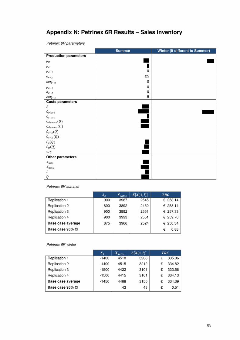
85
Appendix N: Petrinex 6R Results – Sales inventory
Petrinex 6R parameters
Summer Winter (if different to Summer)
Production parameters
�� '''''''' ''''''''''
� ''' �<�� 0
®<�� 25
&$%<�� 0
�<� 0
®<� 0
&$%<� 5
Costs parameters
" ''''''''''
fZ� @ '''''''''''''''' ''''''''''''''''' ����e ''' �<���(�) ''''''''''''
�<���(�) ''''''''''''
��(�)
��(�)
�(�) ''''''
�(�) '''''''
L ''''''''''
Other parameters
���� '''''''''
���� ''''''''''''
2 ''''''
� '''''''''''
Petrinex 6R summer
¬ ËÌÍ¥ ÑJË(Ò, Í)K ÓÔ¡
Replication 1 900 3987 2545 € 258.14
Replication 2 800 3892 2450 € 258.14
Replication 3 900 3992 2551 € 257.33
Replication 4 900 3993 2551 € 259.76
Base case average 875 3966 2524 € 258.34
Base case 95% CI € 0.88
Petrinex 6R winter
¬ ËÌÍ¥ ÑJË(Ò, Í)K ÓÔ¡
Replication 1 -1400 4518 3208 € 335.06
Replication 2 -1400 4515 3212 € 334.82
Replication 3 -1500 4422 3101 € 333.56
Replication 4 -1500 4415 3101 € 334.13
Base case average -1450 4468 3155 € 334.39
Base case 95% CI 43 48 € 0.51

86
Lead time sensitivity analysis summer
¬ ËÌÍ¥ ÑJË(Ò, Í)K ÓÔ¡ Delta TRC
L = 20 1800 3839 2395 € 242.85 -6.02%
L = 25 1300 3865 2422 € 250.48 -3.07%
L = 30 900 3992 2551 € 257.33 -0.42%
L = 35 400 4012 2573 € 264.97 2.54%
L = 40 0 4163 2653 € 270.35 4.62%
Lead time sensitivity analysis winter
¬ ËÌÍ¥ ÑJË(Ò, Í)K ÓÔ¡ Delta TRC
L = 20 300 4221 2889 € 303.78 -9.16%
L = 25 -600 4314 2990 € 317.89 -4.94%
L = 30 -1500 4422 3101 € 333.56 -0.25%
L = 35 -2300 4610 3313 € 344.80 3.11%
L = 40 -3200 4715 3421 € 357.98 7.05%
Tank size sensitivity analysis summer
¬ ËÌÍ¥ ÑJË(Ò, Í)K ÓÔ¡ Delta TRC
Q = X_max = 5600 800 3892 2450 € 258.48 0.03%
3000 X_max = 6600 900 3986 2545 € 258.88 0.18%
X_max = 7600 900 3985 2547 € 258.62 0.08%
X_max = 8600 900 3993 2551 € 259.76 0.52%
X_max = 9600 800 3888 2445 € 257.18 -0.48%
Q = X_max = 5600 1700 4802 2817 € 308.55 19.44%
4000 X_max = 6600 1800 4914 2927 € 300.83 16.45%
X_max = 7600 1800 4908 2922 € 301.13 16.56%
X_max = 8600 1800 4906 2923 € 300.60 16.36%
X_max = 9600 1800 4905 2922 € 301.82 16.83%
Q = X_max = 11000 7300 10676 5620 € 671.81 160.05%
10000 X_max = 12000 7700 10803 5719 € 572.20 121.49%
X_max = 13000 7700 10806 5724 € 573.46 121.98%
X_max = 14000 7700 10805 5721 € 572.75 121.70%
X_max = 15000 7700 10809 5720 € 572.02 121.42%
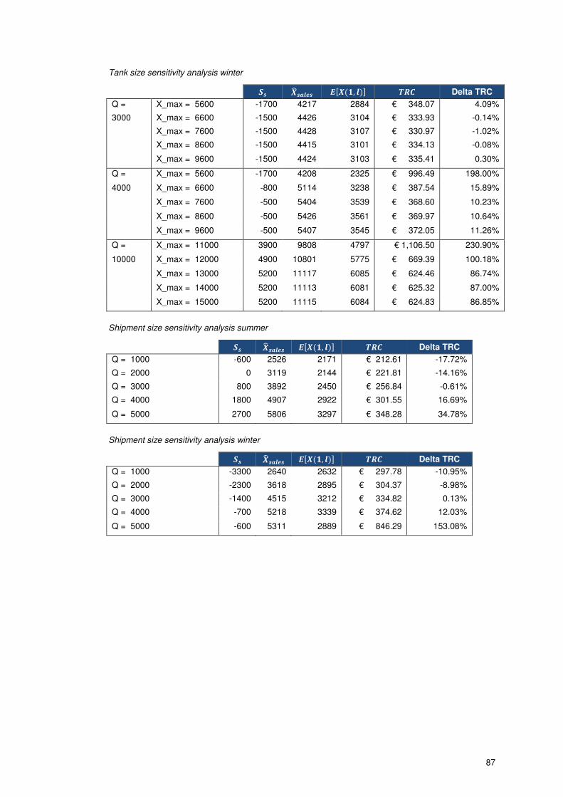
87
Tank size sensitivity analysis winter
¬ ËÌÍ¥ ÑJË(Ò, Í)K ÓÔ¡ Delta TRC
Q = X_max = 5600 -1700 4217 2884 € 348.07 4.09%
3000 X_max = 6600 -1500 4426 3104 € 333.93 -0.14%
X_max = 7600 -1500 4428 3107 € 330.97 -1.02%
X_max = 8600 -1500 4415 3101 € 334.13 -0.08%
X_max = 9600 -1500 4424 3103 € 335.41 0.30%
Q = X_max = 5600 -1700 4208 2325 € 996.49 198.00%
4000 X_max = 6600 -800 5114 3238 € 387.54 15.89%
X_max = 7600 -500 5404 3539 € 368.60 10.23%
X_max = 8600 -500 5426 3561 € 369.97 10.64%
X_max = 9600 -500 5407 3545 € 372.05 11.26%
Q = X_max = 11000 3900 9808 4797 € 1,106.50 230.90%
10000 X_max = 12000 4900 10801 5775 € 669.39 100.18%
X_max = 13000 5200 11117 6085 € 624.46 86.74%
X_max = 14000 5200 11113 6081 € 625.32 87.00%
X_max = 15000 5200 11115 6084 € 624.83 86.85%
Shipment size sensitivity analysis summer
¬ ËÌÍ¥ ÑJË(Ò, Í)K ÓÔ¡ Delta TRC
Q = 1000 -600 2526 2171 € 212.61 -17.72%
Q = 2000 0 3119 2144 € 221.81 -14.16%
Q = 3000 800 3892 2450 € 256.84 -0.61%
Q = 4000 1800 4907 2922 € 301.55 16.69%
Q = 5000 2700 5806 3297 € 348.28 34.78%
Shipment size sensitivity analysis winter
¬ ËÌÍ¥ ÑJË(Ò, Í)K ÓÔ¡ Delta TRC
Q = 1000 -3300 2640 2632 € 297.78 -10.95%
Q = 2000 -2300 3618 2895 € 304.37 -8.98%
Q = 3000 -1400 4515 3212 € 334.82 0.13%
Q = 4000 -700 5218 3339 € 374.62 12.03%
Q = 5000 -600 5311 2889 € 846.29 153.08%

88
Appendix O: Benzene Heartcut Results – Feed inventory
Benzene Heartcut parameters
Summer Winter (if different to Winter)
Production parameters
�� '''
� ''''''''' ''''''''' �<�� 0
®<�� 0
&$%<�� 1
�<� 6
®<� 45
&$%<� 0
Costs parameters
" ''''''''
fZ� @ ''' ����e '''''''''''''' �<���(�) ''''''''''''''''
�<���(�) ''''''''''''''''
��(�)
��(�)
�(�) ''''''''''''
�(�) '''''''''''
L '''''''''''
Other parameters
���� ''''''''''''''''
���� ''''''''''''
2 ''''''
� ''''''''''''
Heartcut Summer
¬¢ Ë¢ÎϧРÑJË(Ò, Í)K ÓÔ¡
Replication 1 13500 5924 9105 € 1,619.01
Replication 2 13500 5930 9121 € 1,658.45
Replication 3 13500 5917 9107 € 1,656.01
Replication 4 13500 5929 9123 € 1,658.83
Base case average 13500 5925 9114 € 1,648.07
Base case 95% CI € 14.74

89
Heartcut Winter
¬¢ Ë¢ÎϧРÑJË(Ò, Í)K ÓÔ¡
Replication 1 8500 4603 7575 € 1,376.89
Replication 2 8500 4592 7560 € 1,379.24
Replication 3 8500 4585 7555 € 1,378.38
Replication 4 8500 4597 7567 € 1,385.40
Base case average 8500 4594 7564 € 1,379.98
Base case 95% CI € 2.84
Lead time sensitivity analysis summer
¬¢ Ë¢ÎϧРÑJË(Ò, Í)K ÓÔ¡ Delta TRC
L = 20 9000 5262 8393 € 1,529.00 -7.23%
L = 25 11500 5839 9018 € 1,603.51 -2.70%
L = 30 13500 5917 9107 € 1,656.01 0.48%
L = 35 15500 5991 9180 € 1,632.28 -0.96%
L = 40 17500 6077 9266 € 1,720.96 4.42%
Lead time sensitivity analysis winter
¬¢ Ë¢ÎϧРÑJË(Ò, Í)K ÓÔ¡ Delta TRC
L = 10 6500 4568 7547 € 1,351.93 -2.03%
L = 15 7500 4590 7564 € 1,364.94 -1.09%
L = 20 8500 4585 7555 € 1,378.38 -0.12%
L = 25 9500 4615 7577 € 1,392.19 0.88%
L = 30 10500 4617 7574 € 1,406.67 1.93%
Tank size sensitivity analysis summer
¬¢ Ë¢ÎϧРÑJË(Ò, Í)K ÓÔ¡ Delta TRC
Q = X_max = 10500 12500 5016 8310 € 2,120.98 28.69%
5000 X_max = 15500 13500 5916 9109 € 1,656.39 0.50%
X_max = 20500 13500 5942 9128 € 1,622.99 -1.52%
X_max = 25500 13500 5929 9123 € 1,658.83 0.65%
X_max = 30500 13500 5936 9118 € 1,621.19 -1.63%
Q = X_max = 10500 11000 6068 9690 € 7,045.50 327.50%
10000 X_max = 15500 12500 4946 10617 € 2,213.00 34.28%
X_max = 20500 13000 5427 11151 € 2,040.18 23.79%
X_max = 25500 13000 5420 11147 € 2,020.37 22.59%
X_max = 30500 13000 5425 11152 € 2,021.19 22.64%

90
Tank size sensitivity analysis winter
¬¢ Ë¢ÎϧРÑJË(Ò, Í)K ÓÔ¡ Delta TRC
Q = X_max = 10500 8500 4602 7569 € 1,383.61 0.26%
5000 X_max = 15500 8500 4603 7565 € 1,375.10 -0.35%
X_max = 20500 8500 4598 7563 € 1,379.73 -0.02%
X_max = 25500 8500 4597 7567 € 1,385.40 0.39%
X_max = 30500 8500 4595 7566 € 1,380.21 0.02%
Q = X_max = 10500 5000 4000 6853 € 4,405.11 219.22%
10000 X_max = 15500 8000 4207 9656 € 1,807.28 30.96%
X_max = 20500 8000 4215 9670 € 1,804.95 30.80%
X_max = 25500 8000 4206 9662 € 1,808.46 31.05%
X_max = 30500 8000 4207 9656 € 1,804.97 30.80%
Shipment size sensitivity analysis summer
¬¢ Ë¢ÎϧРÑJË(Ò, Í)K ÓÔ¡ Delta TRC
Q = 2500 13500 5935 8258 € 1,468.32 -10.91%
Q = 5000 13500 5930 9121 € 1,658.45 0.63%
Q = 7500 13000 5410 9889 € 1,836.05 11.41%
Q = 10000 13000 5428 11153 € 2,059.55 24.97%
Q = 12500 13000 5429 12454 € 2,244.74 36.20%
Shipment size sensitivity analysis winter
¬¢ Ë¢ÎϧРÑJË(Ò, Í)K ÓÔ¡ Delta TRC
Q = 2500 8500 4602 6386 € 1,225.51 -11.19%
Q = 5000 8500 4592 7560 € 1,379.24 -0.05%
Q = 7500 8500 4590 8802 € 1,584.45 14.82%
Q = 10000 8000 4201 9645 € 1,810.28 31.18%
Q = 12500 8000 4203 11033 € 2,024.69 46.72%

91
Appendix P: Existence of Ss and Sp
Short buffer:
�� = 500
� = 550
Small FCE
©¥�¢ = ©¥�§ = «%
Large FCE
©¥�¢ = ©¥�§ = ª«%
 ¢  ¢
Small Q
£ = ÒÕÕÕ 10^9
2300
(€ 563) 10^9
3900
(€ 1077)
Large Q
£ = ÖÕÕÕ 10^9
2300
(€ 874) 10^9
3100
(€ 2289)
�� = 500
� = 750
Small FCE
©¥�¢ = ©¥�§ = «%
Large FCE
©¥�¢ = ©¥�§ = ª«%
 ¢  ¢
Small Q
£ = ÒÕÕÕ 10^9
4400
(€ 684) 10^9
6300
(€ 1380)
Large Q
£ = ÖÕÕÕ 10^9
4400
(€ 917) 10^9
5500
(€ 2843)
Long buffer:
�� = 550
� = 500
Small FCE
©¥�¢ = ©¥�§ = «%
Large FCE
©¥�¢ = ©¥�§ = ª«%
 ¢  ¢
Small Q
£ = ÒÕÕÕ
2300
(€ 543) -10^9
4500
(€ 1128) 1700
Large Q
£ = ÖÕÕÕ
5300
(€ 829) -10^9
6400
(€ 2126) -10^9
�� = 750
� = 500
Small FCE
©¥�¢ = ©¥�§ = «%
Large FCE
©¥�¢ = ©¥�§ = ª«%
 ¢  ¢
Small Q
£ = ÒÕÕÕ
1500
(€ 962) -10^9
2600
(€ 1405) -10^9
Large Q
£ = ÖÕÕÕ
3400
(€ 927) -10^9
4100
(€ 2998) -10^9

92
Appendix Q: Transient vs. Simulation model
Balanced buffer analyses:
fZ� @ = ′′′′′′′′′′′′′′′ ���(�) = ′′′′′′′′′′′′′ ����e = ′′′′′′′′′′′′′′′′ �(�) = ′′′′′′′′ ��(�) = ′′′′′′′′′′′′ �(�) = ′′′′′′′′ �(0) = ���� + ���� − ����2 = 4.800
�� = 500
� = 500 Transient
Simulation
©¥�¢ = ©¥�§ = ª«%
 ¢  ¢
Small Q
£ = ÒÕÕÕ
10^9
(€ 1304)
1600
10^9
(€ 1141) -10^9
Large Q
£ = ÖÕÕÕ
10^9
(€ 1308) 1600
10^9
(€ 1154) -10^9
Q=1000:
Q=4000:
0
5000
10000
15000
20000
25000
30000
TR
C
Sales / Purchase level
Ss - Sim
Ss - Trans
Sp - Trans
Sp - Trans
0
10000
20000
30000
40000
50000
60000
70000
80000
90000
TR
C
Sales / Purchase level
Ss - Sim
Ss - Trans
Sp - Trans
Sp - Trans

93
fZ� @ = ′′′′′′′′′′′′′′ ���(�) = 0
����e = ′′′′′′′′′′′′′′′′′ �(�) = 0
��(�) = 0 �(�) = 0
�(0) = ���� + ���� − ����2 = 4.800
�� = 500
� = 500 Transient
Simulation
©¥�¢ = ©¥�§ = ª«%
 ¢  ¢
Small Q
£ = ÒÕÕÕ
5200
(€ 1147) 3900
5000
(€ 1068) 3500
Large Q
£ = ÖÕÕÕ
6900
(€ 1290) 2400
6600
(€ 1138) 2200
Q=1000:
Q=4000:
0
2000
4000
6000
8000
10000
12000
14000
16000
TR
C
Sales / Purchase level
Ss - Sim
Ss - Trans
Sp - Trans
Sp - Trans
0
2000
4000
6000
8000
10000
12000
14000
16000
18000
20000
TR
C
Sales / Purchase level
Ss - Sim
Ss - Trans
Sp - Trans
Sp - Trans