
Eindhoven University of Technology MASTER A ray tracing ...
83
Eindhoven University of Technology MASTER A ray tracing approach to computational electromagnetics for reverberation chambers Nauwelaerts, F. Award date: 2009 Link to publication Disclaimer This document contains a student thesis (bachelor's or master's), as authored by a student at Eindhoven University of Technology. Student theses are made available in the TU/e repository upon obtaining the required degree. The grade received is not published on the document as presented in the repository. The required complexity or quality of research of student theses may vary by program, and the required minimum study period may vary in duration. General rights Copyright and moral rights for the publications made accessible in the public portal are retained by the authors and/or other copyright owners and it is a condition of accessing publications that users recognise and abide by the legal requirements associated with these rights. • Users may download and print one copy of any publication from the public portal for the purpose of private study or research. • You may not further distribute the material or use it for any profit-making activity or commercial gain
Transcript of Eindhoven University of Technology MASTER A ray tracing ...
Eindhoven University of Technology
MASTER
A ray tracing approach to computational electromagnetics for reverberation chambers
Nauwelaerts, F.
Award date:2009
Link to publication
DisclaimerThis document contains a student thesis (bachelor's or master's), as authored by a student at Eindhoven University of Technology. Studenttheses are made available in the TU/e repository upon obtaining the required degree. The grade received is not published on the documentas presented in the repository. The required complexity or quality of research of student theses may vary by program, and the requiredminimum study period may vary in duration.
General rightsCopyright and moral rights for the publications made accessible in the public portal are retained by the authors and/or other copyright ownersand it is a condition of accessing publications that users recognise and abide by the legal requirements associated with these rights.
• Users may download and print one copy of any publication from the public portal for the purpose of private study or research. • You may not further distribute the material or use it for any profit-making activity or commercial gain

TECHNISCHE UNIVERSITEIT EINDHOVEN
Department of Mathematics and Computer Science
MASTER THESIS
A ray tracing approach to computational electromagnetics
for reverberation chambers
by
F.Nauwelaerts
Supervisors: dr. A.T.M. Aerts
dr. ir. D. Van Troyen
Eindhoven, December 2008


A ray tracing approach to computational electromagnetics for reverberation chambers
Preface This Master Thesis finalizes my studies at the Department of Mathematics and Computer Science at the Eindhoven University of Technology. I have experienced these last few years as a journey, where I have encountered several challenging situations and several very interesting people. In my own perception, the destination which this Master Thesis once was, has now become a starting point for further personal development. I would like to thank my supervisor during the development of this Thesis, Ad Aerts, for his mind-opening suggestions, very useful input during this project and the interesting conversations we had. I also wish to express my sincere gratitude to Dirk Van Troyen, Laboratoria De Nayer supervisor. Not only for the guidance and elaborated answers on each and every question, but also for the essential support given throughout my entire study. My gratitude also goes to my future wife, Micheline, who encouraged me whenever needed and endured my ‘time-sharing’ between job, studies and personal time. Finally, I want to thank my parents, friends, family and colleagues, for their direct or indirect help whenever needed. Filip Nauwelaerts
3

A ray tracing approach to computational electromagnetics for reverberation chambers
Index 1 Introduction ......................................................................................................................................8
1.1 Context description ....................................................................................................................8 1.2 Immunity assessment .................................................................................................................8 1.3 Field uniformity .........................................................................................................................9
2 Objectives .......................................................................................................................................11 3 Simulation application....................................................................................................................12
3.1 Conceptual description.............................................................................................................12 3.2 The ray tracing process ............................................................................................................13
3.2.1 Ray surface intersection calculations..............................................................................14 3.2.2 Individual ray generation................................................................................................18 3.2.3 Ray reflection .................................................................................................................20 3.2.4 Spatial subdivision..........................................................................................................21
3.3 Electromagnetic propagation....................................................................................................28 3.3.1 Field equations of a Hertz dipole in free space...............................................................28 3.3.2 Radiation of a linear antenna ..........................................................................................32 3.3.3 Reflection of electromagnetic waves ..............................................................................34
3.4 When ray tracing and EM propagation meet............................................................................39 4 Validation of the simulation application.........................................................................................41
4.1 Single direct and reflected ray intersection inside a semi-anechoic chamber ..........................41 4.1.1 Description......................................................................................................................41 4.1.2 Simulation goal...............................................................................................................41 4.1.3 Simulation results ...........................................................................................................41
4.2 A standing wave pattern...........................................................................................................44 4.2.1 Description......................................................................................................................44 4.2.2 Simulation goal...............................................................................................................44 4.2.3 Simulation results ...........................................................................................................44
4.3 A fundamental TE10 mode simulation inside a rectangular waveguide....................................46 4.3.1 Description......................................................................................................................46 4.3.2 Simulation goal...............................................................................................................47 4.3.3 Simulation results ...........................................................................................................47
4.4 Effects of an aperture inside a rectangular waveguide .............................................................49 4.4.1 Description......................................................................................................................49 4.4.2 Simulation goal...............................................................................................................50 4.4.3 Simulation results ...........................................................................................................50
4.5 Simulating a higher TE mode inside a rectangular waveguide ................................................51 4.5.1 Description......................................................................................................................51 4.5.2 Simulation goal...............................................................................................................51 4.5.3 Simulation results ...........................................................................................................51
4.6 Field evaluation inside a large reverberation chamber .............................................................53 4.6.1 Description......................................................................................................................53 4.6.2 Simulation goal...............................................................................................................54 4.6.3 Simulation results ...........................................................................................................54
5 Conclusion......................................................................................................................................58 5.1 General conclusion...................................................................................................................58 5.2 Results analysis ........................................................................................................................58
5.2.1 Can the field uniformity be determined? ........................................................................58 5.2.2 Accuracy.........................................................................................................................58
5.3 Future work ..............................................................................................................................60 5.4 Design process analysis............................................................................................................61
6 References ......................................................................................................................................62 Appendix A ............................................................................................................................................63
A.1 An example of ray and plane intersection ...........................................................................63 Appendix B.............................................................................................................................................64
B.1 Derivation of equations for E and H in a Cartesian system.................................................64 B.2 Derivation of EZ equation in terms of magnetic vector potential ........................................65 B.3 Simplification of HΦ equation for far field conditions.........................................................65 B.4 Vector potential equation for half wavelength dipole .........................................................65
Appendix C.............................................................................................................................................67
4

A ray tracing approach to computational electromagnetics for reverberation chambers
1. Defining chamber properties ...............................................................................................67 2. Transmit antenna and cell group settings ............................................................................67 3. Simulation project settings ..................................................................................................68 4. Vector field visualization ....................................................................................................69
Appendix D ............................................................................................................................................71 1. Context Analysis of the immunity assessment application ......................................................71 2. Requirement Analysis ..............................................................................................................72
2.1. User requirements................................................................................................................72 3. Application Model ...................................................................................................................73
3.1. Object model .......................................................................................................................73 3.2. Process models for Use Cases .............................................................................................74
4. Design and implementation......................................................................................................77 4.1. Design model.......................................................................................................................77 4.2. Implementation....................................................................................................................78
5

A ray tracing approach to computational electromagnetics for reverberation chambers
Table of Figures Figure 1: Example of reverberation chamber ..........................................................................................9 Figure 2: Reverberation chamber test volume .......................................................................................10 Figure 3: Conceptual description...........................................................................................................12 Figure 4: Ray tracing technique for 2D screen ......................................................................................13 Figure 5: Ray tracing technique for 2D screen ......................................................................................13 Figure 6: Cartesian coordinates of two points .......................................................................................14 Figure 7: Ray equation unit vector.........................................................................................................15 Figure 8: Determination of a surface normal ........................................................................................15 Figure 9: Distance to plane intersection ................................................................................................16 Figure 10: Intersection inside or outside panel.....................................................................................17 Figure 11: Inside or outside verification ................................................................................................17 Figure 12: spherical ray generation.......................................................................................................18 Figure 13: Rotation step angle ...............................................................................................................18 Figure 14: Individual ray identification .................................................................................................18 Figure 15: Tuned dipole radiation pattern.............................................................................................19 Figure 16: Antenna radiation pattern and ray generation .....................................................................20 Figure 17: Individual ray identification .................................................................................................20 Figure 18: Multiple measurement points ...............................................................................................21 Figure 19: Reference points missed .......................................................................................................21 Figure 20: Spatial subdivision as a solution to missed reference points................................................22 Figure 21: close-up of intersected cell ...................................................................................................22 Figure 22: Identification of intersected cell(s) .......................................................................................23 Figure 23: Cell group divided by planes ................................................................................................23 Figure 24: Facet intersection .................................................................................................................24 Figure 25: Identifying intersected cell facet(x direction) .......................................................................24 Figure 26: Identifying intersected cell facet(y and z direction)..............................................................24 Figure 27: Intersection with multiple cells.............................................................................................25 Figure 28: Close up of intersection with multiple cells ..........................................................................25 Figure 29: Flowchart for the determination of individual cell contribution ..........................................26 Figure 30: Wave fronts consist of different rays ....................................................................................27 Figure 31: 4 rays for 2 wave fronts ........................................................................................................27 Figure 32: Electromagnetic propagation ...............................................................................................28 Figure 33: Current distribution assumption...........................................................................................29 Figure 34: Vector potential for a Hertz dipole.......................................................................................29 Figure 35: Vector decomposition for a spherical-polar coordinate system ..........................................30 Figure 36: Electric and magnetic field vectors for a spherical-polar coordinate system ......................31 Figure 37: Near field and far field distinction .......................................................................................32 Figure 38: Current distribution for a half wave dipole ..........................................................................33 Figure 39: Spectral reflection ................................................................................................................34 Figure 40: Plane of incidence ................................................................................................................35 Figure 41: Polarization of field vector before and after spectral reflection ..........................................35 Figure 42: Horizontal component of field vector before and after reflection .......................................36 Figure 43: Vertical component of field vector before and after reflection............................................37 Figure 44: Horizontal unit vector...........................................................................................................37 Figure 45: Vertical unit vector ...............................................................................................................37 Figure 46: Determination of vertical field component after reflection by vector calculus ....................38 Figure 47: Brief overview of the ray tracing algorithm .........................................................................40 Figure 48: Simulation result – reflected and direct path intersection....................................................41 Figure 49: Simulation result – ray attenuation evaluation ....................................................................42 Figure 50: Simulation result – ray reflection evaluation .......................................................................42 Figure 51: Simulation result – close-up of ray reflection.......................................................................43 Figure 52: Simulation result – ray intersection evaluation ....................................................................43 Figure 53: Simulation result – close-up of ray intersection ...................................................................44 Figure 54: Simulation result – Standing wave pattern ...........................................................................45 Figure 55: Simulation result – direct and reflected wave decomposition ..............................................45 Figure 56: Simulation result – influence of cell sizes.............................................................................46 Figure 57: Wave guide dimensions ........................................................................................................46
6

A ray tracing approach to computational electromagnetics for reverberation chambers
Figure 58: Wave guide dimensions – side view......................................................................................46 Figure 59: internal angle of incidence ...................................................................................................47 Figure 60: simulation result of a wave guide TE1,0 mode.......................................................................47 Figure 61: simulation result of a wave guide TE1,0 mode- side view......................................................48 Figure 62: simulation result of a wave guide TE1,0 mode- top view .......................................................48 Figure 63: Ray contribution inside waveguide, Ө1 ................................................................................49 Figure 64: ray contribution inside waveguide, Ө2 .................................................................................49 Figure 65: Aperture inside waveguide ...................................................................................................50 Figure 66: Aperture inside waveguide – 3D simulation result...............................................................50 Figure 67: Aperture inside waveguide – top view of simulation result .................................................50 Figure 68: Next mode inside waveguide – top view of simulation results..............................................51 Figure 69: section 1 in 3D view .............................................................................................................51 Figure 70: Waveguide TE50 mode ..........................................................................................................52 Figure 71: TE50 mode at front-end .........................................................................................................52 Figure 72: TE50 mode along the waveguide ...........................................................................................52 Figure 73: Reverberation chamber simulation – setup 1 ......................................................................53 Figure 74: Field probe ...........................................................................................................................53 Figure 75: Transmitting dipole ..............................................................................................................53 Figure 76: Reverberation chamber simulation – setup 2 ......................................................................54 Figure 77: Setup 1 and 2 – dipole and probe locations .........................................................................54 Figure 78: Exyz for setup 1 ....................................................................................................................55 Figure 79: Exyz for setup 2 ....................................................................................................................55 Figure 80: Ex for setup 1........................................................................................................................55 Figure 81: Ey for setup 1........................................................................................................................55 Figure 82: Ez for setup 1........................................................................................................................55 Figure 83: Ex for setup 2........................................................................................................................55 Figure 84: Ey for setup 2........................................................................................................................55 Figure 85: Ez for setup 2........................................................................................................................55 Figure 86: Histogram field vector amplitude for setup 1 and 2 .............................................................56 Figure 87: Determination or the minimal angle step .............................................................................59 Figure 88: example of ray/plane intersection.........................................................................................63 Figure 89: difference in traveling distance for each individual Hertz dipole ........................................66 Figure 90: User interface - quantification of chamber properties .........................................................67 Figure 91: User interface –transmit antenna and cell group settings....................................................68 Figure 92: User interface – initialization of a simulation ......................................................................69 Figure 93: Second alternative: quiver3 function....................................................................................69 Figure 94: third alternative: surf function for a group of cells with identical z-index...........................70 Figure 95: Selection of test equipment,e.g. generators ..........................................................................71 Figure 96: Object Model ........................................................................................................................74 Figure 97: use case – adding device ......................................................................................................74 Figure 98: use case – deleting device.....................................................................................................75 Figure 99: use case – changing device parameters................................................................................75 Figure 100: use case – immunity test setup ............................................................................................76 Figure 101: use case – Running an immunity test..................................................................................77 Figure 102: design model.......................................................................................................................77 Figure 103: HW Interface ......................................................................................................................79 Figure 104: RI test setup interface .........................................................................................................80 Figure 105: RI device selection interface...............................................................................................80 Figure 106: RI test run interface ............................................................................................................81
7

A ray tracing approach to computational electromagnetics for reverberation chambers
1 Introduction
1.1 Context description All products which are commercially available within the European market are required to comply with all relevant European directives. For electronic products, one of the most important directives is the EMC directive 2004/108/EG, which contains essential requirements on the field of electromagnetic compatibility amongst different electronic applications [EMC1]. In order to demonstrate compliance with this EMC directive, the responsible distributors need to perform an EMC assessment. This assessment contains a series of measurements, which each in turn cover a relevant physical EMC behavior of the device, either by verifying the immunity of the device to specified EM stresses (e.g. disturbance fields) as well as by verifying the emission of the device (e.g. radiation). In case all the necessary tests are successfully passed, it is allowed to declare conformity with the EMC directive. One specific measurement during an EMC assessment requires immunity of the device towards radiated EM fields. In order to proof a sufficient immunity level, the device is placed inside an environment where a specific electromagnetic disturbance field is created in a controlled manner by the use of an antenna. The different functionalities of the device are verified while this field is applied [GOE1]. There are different standards which describe how this immunity measurement needs to be performed. Within the scope of this project, the relevant standards are DO160, IEC 61000-4-21, MILSTD 461E and SAE J551/J113, which describe the use of a reverberation chamber [DO160, IEC421]. A reverberation chamber consists of a cage of Faraday, where the walls on the inside are characterized by a very low absorption rate towards electromagnetic energy [MPI1, HOL1]. This means that the walls will have a very high reflecting effect on incident electromagnetic fields. These reflections will cause standing wave patterns within the chambers’ cavity, in function of the source antennas’ position and the distances between reflecting walls and the antenna. This standing wave pattern and its associated resonant effects allow the creation of very high field strength (measured in V/m) with moderate input power to the source antenna. The disadvantage is that the conditions for this resonant effect are limited in the frequency spectrum; due to the fixed dimensions of the test chamber and the fixed location of the source antenna, resonance will occur only for a limited number of frequency bands within the entire spectrum of interest. To cope with this limitation, a mode stirrer is used. The mode stirrer consists of a rotating axis, on to which several reflecting panels are attached. During the creation of the high level EM fields, the mode stirrer will be turned over 360 deg. By doing this, it is possible to change the distances between different reflecting panels, causing a shift in the frequency bands for which a resonance inside the test chamber occurs. Provided a good design of the mode stirrer, a sufficient resonant pattern can be obtained within the complete frequency spectrum of our interest (80MHz up to 26GHz). Also, the mode stirrer will provide a stochastic distribution of field polarizations, which means that the device under test will be subjected to different EM field polarizations at the same time.
1.2 Immunity assessment When performing an immunity assessment, different test equipment will be used to generate a controlled electromagnetic field; a function generator will be used to generate a repetitive waveform, with a defined amplitude and frequency and possibly modulated (AM, PM). After
8

A ray tracing approach to computational electromagnetics for reverberation chambers
amplification, the output signal of the generator will serve as an input signal to a specific antenna, which in turn generates the required electromagnetic field. The frequency of the generated waveform will be increased in a stepwise manner. For each of these frequencies, a complete stirrer rotation will ensure a maximum resonant effect inside the reverberation chamber. This rotation of the mode stirrer will be performed with discrete stirrer rotation steps, which means that the stirrer will be positioned at a finite number of angles during a specified dwell time. This method is referred to as mode stirring. The number of angles within one complete rotation is frequency dependant, and should be chosen in such a way that it will compensate a lower amount of resonant modes inside the reverberation chamber. Near the test object, the EM field level is monitored by means of a field probe or receive antenna. The immunity assessment requires simultaneous control and monitoring of a variety of test equipment. Any inaccuracy in the control of this test equipment might result in over or under testing of the test object, which is of course intolerable. The urgency for an automated assessment application is eminently clear. An immunity measurement application will not only fulfill these requirements, but it will also provide the possibility to restrict the test engineers actions in order to avoid or minimize potential manipulation errors during the initialization of an immunity test. Within the first part of this project, it is requested to design and implement an application which will indeed enable automated immunity assessment.
Mode stirrer
Height
Figure 1: Example of reverberation chamber
1.3 Field uniformity Before the usage of a reverberation chamber for radiated immunity testing is allowed (e.g. in conformance with EN61000-4-21), certain specifications or criteria of the chamber need to be met. Some of these criteria depend on the structure of the chamber and mode stirrer itself. For example, the lowest usable frequency for a certain chamber depends on the chamber dimensions and the mode stirrer efficiency. These parameters in turn determine the number of resonant modes which occur within the lowest frequency band. Another criterion is field homogeneity or field uniformity. When radiated immunity tests are performed, the device under test must be placed within a cubicle shaped test volume, for which both dimensions and location are defined in function of the lowest usable frequency of the chamber. The field uniformity criterion states that the field strength, measured at the eight corner points of the test volume (and for each polarization respectively), lies within a specified standard deviation from the normalized mean value of the normalized maximum values obtained at each of the eight locations, during one rotation of the mode stirrer (4dB from the LUF up to 100MHz and 3dB from 400MHz up to the maximal frequency). In other words, these 24 values must fall within 4 or 3dB for each frequency, otherwise the reverberation chamber may not be used as a valid test method.
9

A ray tracing approach to computational electromagnetics for reverberation chambers
The EN61000-4-21 standard describes a method to verify the field uniformity criterion, based on a series of measurements. More details on this procedure can be found in the referred standard, the interested reader will come to the conclusion that it takes a lot of measurement time before it can be concluded whether or not the reverberation chamber may be used as a valid method for radiated immunity testing of a certain device. Especially when the reverberation chamber is used within a commercial context where time still is money, an alternative ‘fast’ method would be useful. This in fact leads to the primary goal of a simulation application: prediction of the influence of a specific device on the chamber loading (i.e. field uniformity), without having to perform an entire chain of measurements, as described above.
1
4
8 7
2
3
6 5
Reverberation chamber
Test volume
Figure 2: Reverberation chamber test volume
In Chapter 0, a summary of the objectives for this project is given. Based on the given context description in this chapter, some general questions are asked, leading to answers which can be translated into requirements for the application. At the end of this document, it is verified whether the proposed solutions and used techniques will indeed sufficiently meet these requirements. Chapter 3 describes a theoretical background on the applied ray tracing technique and design issues for the simulation application. Chapter Fout! Verwijzingsbron niet gevonden. presents the results of a set of validation cases, where the results of the simulation application are verified for accuracy and reliability. The test cases are chosen in such a way that the most important aspects of the simulation application are verified. A conclusion is given in Chapter 5, together with propositions for future work on this project. In the course of this Master thesis project also an immunity assessment application was developed. This application automates the assessment process and supports a test engineer to set up and run immunity tests. During set up the engineer can specify the equipment to be used and the parameters to be set. The application stores the test specifications such that they can be reused. It requires less theoretical background and its description is therefore rather straightforward. Since this application is rather independent of the simulation topic its description has been delegated to Appendix D where a context and requirements analysis and an application model are given.
10

A ray tracing approach to computational electromagnetics for reverberation chambers
2 Objectives
Q: How to verify field uniformity without having to perform long term measurements? During radiated immunity tests, the field uniformity needs to be maintained when a test object is put in place within the test volume boundaries. EN61000-4-21 for example describes a method to verify field uniformity, based on a series of measurements. These measurements take time however, and are performed when the test sample is already put inside the test chamber.
A: An exhaustive set of validation measurements can be avoided if we could simulate the
resulting EM field and predict its behavior. Simulation results can be analyzed and field uniformity can be evaluated. Definition of dimensions and behavior of different test samples, chamber dimensions and mode stirrer positions should be possible.
Q: Which technique should be used for simulating electromagnetic field propagation?
A: Different techniques currently exist to calculate a resulting EM field, such as Boundary
Element Method (BEM) [KKY1], Finite Element Method (FEM), Finite Difference Method (FDM), Finite Difference Time-Domain Method (FDTD), Ray Tracing, etc. All mentioned methods are based on solving partial differential equations, such as the wave equation.
In finite element modeling, the entire interior region of the reverberation chamber will be discretised into finite elements with the reflecting or absorbing effect of the walls acting as boundary conditions. Since the entire 3D region is modeled, the required number of elements is very large. The boundary element method on the other hand only requires discretisation of the boundary walls, and hence requires much less elements then FEM does. Literature shows that BEM provides a theoretical exact formulation and it has been proven to be a highly accurate method for many problems. A disadvantage however can be that this method is computationally demanding to use routinely. In comparison, an advantage of ray tracing is its ease of understanding and its straightforwardness [LAU1]. These arguments lead to the choice of using an adjusted ray tracing technique. The details on the theoretical background and its implementation are discussed in the following chapters. In addition to the theoretical review on existing techniques, two research groups were visited who are currently working on similar projects [FDI1, FOL1, HUB1, LAE1, VLI1, WAL1, WAL2]. These research groups are lead by prof. Van Lil (Katholieke Universiteit Leuven, department ESAT-TELEMIC) and prof. De Zutter (Ghent University) respectively. It was not evident however to find a clear match between the current projects within these groups and the objectives for this project itself, more specific considering the limited time frame of this graduation project.
Q: How can the resulting data enable the validation of a reverberation chamber towards field uniformity?
A: It should be possible to visualize the resulting field strength, in order to have an intuitive
feeling about its characteristic behavior. On the other hand, there should also be a possibility to access the raw data, which enables a more numerical approach and data manipulation, which in turn enables validation of the reverberation chamber for its field uniformity.
Q: How to maximize the accuracy and reliability of the chosen method?
A: The chosen method is an adapted ray tracing technique. It is shown in the following chapters
that this method is adapted in such a way that the end user can influence the accuracy of the final result. This can be done by choosing sufficiently small cell sizes (Section 3.2.4 on p.21) and sufficiently small angle steps when initial rays are calculated (Section 3.2.2 on p. 18).
11

A ray tracing approach to computational electromagnetics for reverberation chambers
3 Simulation application
3.1 Conceptual description The desired simulation application will have to be designed in such a way that it allows the calculation and visualization of an electromagnetic vector field, which results from electromagnetic propagation inside a specified environment. As mentioned in chapter 0, the choice is made to rely on the ray tracing technique. How this technique is implemented and transformed into a suitable algorithm is described into more detail in sections 3.2. Generally speaking, the ray tracing technique decomposes the propagated electromagnetic wave fronts into a set of distinct rays. For each individual ray, it can be calculated how it propagates through the defined environment and how its path is influenced by obstacles. As a next step, the contribution of each individual ray to the resulting vector field needs to be quantified. By implementation of appropriate equations in the field of electromagnetism, the electric field strength and its polarization can be calculated for each location on an arbitrary ray. Which equations are implemented and how influence of reflections are dealt with, is described in section 3.3. The following model shows how both fields of expertise are combined, and where each of them comes into play. More details about this synergy are given in section 3.4.
Ray path calculations and Potential reflection evaluation
User defined parameters
Calculation of resulting Quantification of corresponding
field strength vectors
Ray tracing
EM propagation
Vector field visualization
vector field
Initialization of rays and environment
Figure 3: Conceptual description
12
A ray tracing approach to computational electromagnetics for reverberation chambers
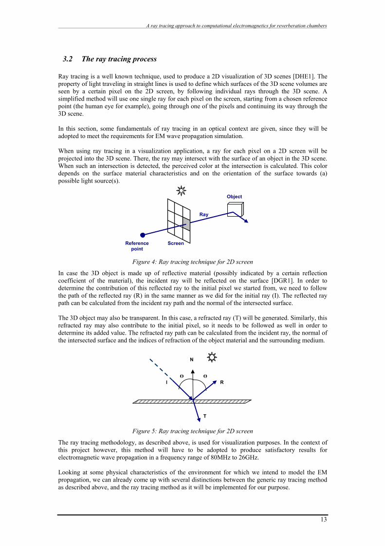
3.2 The ray tracing process Ray tracing is a well known technique, used to produce a 2D visualization of 3D scenes [DHE1]. The property of light traveling in straight lines is used to define which surfaces of the 3D scene volumes are seen by a certain pixel on the 2D screen, by following individual rays through the 3D scene. A simplified method will use one single ray for each pixel on the screen, starting from a chosen reference point (the human eye for example), going through one of the pixels and continuing its way through the 3D scene. In this section, some fundamentals of ray tracing in an optical context are given, since they will be adopted to meet the requirements for EM wave propagation simulation. When using ray tracing in a visualization application, a ray for each pixel on a 2D screen will be projected into the 3D scene. There, the ray may intersect with the surface of an object in the 3D scene. When such an intersection is detected, the perceived color at the intersection is calculated. This color depends on the surface material characteristics and on the orientation of the surface towards (a) possible light source(s).
Reference point
Screen
Object
Ray
Figure 4: Ray tracing technique for 2D screen
In case the 3D object is made up of reflective material (possibly indicated by a certain reflection coefficient of the material), the incident ray will be reflected on the surface [DGR1]. In order to determine the contribution of this reflected ray to the initial pixel we started from, we need to follow the path of the reflected ray (R) in the same manner as we did for the initial ray (I). The reflected ray path can be calculated from the incident ray path and the normal of the intersected surface. The 3D object may also be transparent. In this case, a refracted ray (T) will be generated. Similarly, this refracted ray may also contribute to the initial pixel, so it needs to be followed as well in order to determine its added value. The refracted ray path can be calculated from the incident ray, the normal of the intersected surface and the indices of refraction of the object material and the surrounding medium.
N
I R Ө Ө
T
Figure 5: Ray tracing technique for 2D screen
The ray tracing methodology, as described above, is used for visualization purposes. In the context of this project however, this method will have to be adopted to produce satisfactory results for electromagnetic wave propagation in a frequency range of 80MHz to 26GHz. Looking at some physical characteristics of the environment for which we intend to model the EM propagation, we can already come up with several distinctions between the generic ray tracing method as described above, and the ray tracing method as it will be implemented for our purpose.
13

A ray tracing approach to computational electromagnetics for reverberation chambers
• For example, the surfaces of the walls of the reverberation chamber and of the metallic panels of the mode stirrer have a high reflection coefficient. These surfaces will never be transparent, so no refraction needs to be calculated.
• The reverberation chamber is a closed cavity, which means that every ray path will eventually intersect with a surface.
• Where one or multiple light sources are used in visualization applications, our source is one transmit antenna.
• There will be a limited amount of reflections for each ray. There are more distinctions, but these are each in turn dealt with in the following sections.
3.2.1 Ray surface intersection calculations When focusing on one single ray, we need to be able to calculate in some way at which point this ray will intersect with one of the given surfaces. This can be done if we know a) the ray equation for that specific ray, and b) the plane equation for each existing surface within the cavity of the reverberation chamber. As a mathematical background, we first elaborate possible derivations of the plane and ray equations. a) Basic ray equation
Consider a straight line inside a Cartesian coordinate system. When the coordinates of two points (P0 and P1) on this line are known, we are able to set up an equation for this line, which holds for each point on this line. From Figure 6 we derive the parametric equation ( ℜ∈r )
⎪⎩
⎪⎨
⎧
−+=−+=−+=
)zz.(rzz)yy.(ryy)xx.(rxx
0P1P0P
0P1P0P
0P1P0P
P1P0
xP1
YP0
ZP1
ZP0
xP0 X
Z
Y YP1
Figure 6: Cartesian coordinates of two points
This equation can be transformed into the ray equation, taking following considerations into account:
⎪⎩
⎪⎨
⎧
−+=−+=−+=
)zz.(rzz)yy.(ryy)xx.(rxx
0P1P0P
0P1P0P
0P1P0P
with: P = (x,y,z) an arbitrary
point on the ray P0 = (xP0, yP0, zP0) P1 = (xP1, yP1, zP1)
14
A ray tracing approach to computational electromagnetics for reverberation chambers
≡ P = P0 + r.( P1 – P0)
with: ur = P0) P1 (P0) P1 (
−−
and ℜ∈s
≡ P = P0 + s.ur (1)
Y
Z
X
P1P0
u
Figure 7: Ray equation unit vector
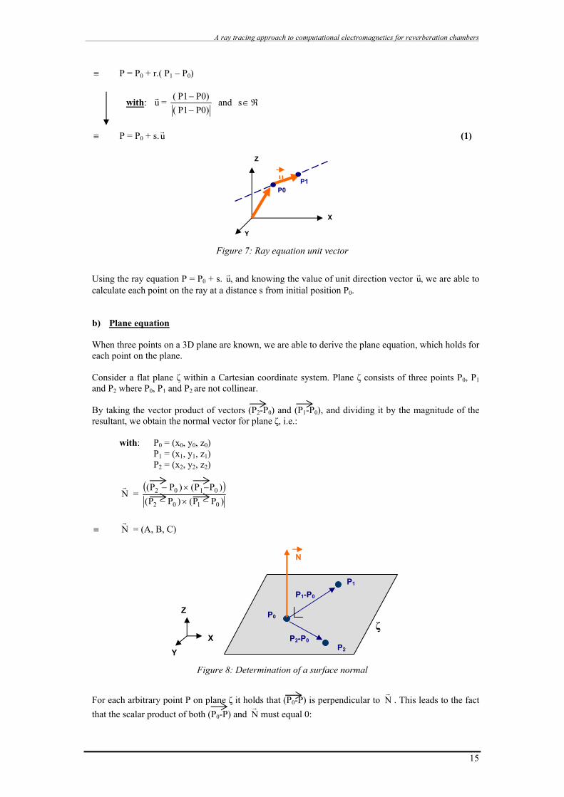
Using the ray equation P = P0 + s. ur, and knowing the value of unit direction vector ur, we are able to calculate each point on the ray at a distance s from initial position P0.
b) Plane equation
When three points on a 3D plane are known, we are able to derive the plane equation, which holds for each point on the plane. Consider a flat plane ζ within a Cartesian coordinate system. Plane ζ consists of three points P0, P1 and P2 where P0, P1 and P2 are not collinear. By taking the vector product of vectors (P2-P0) and (P1-P0), and dividing it by the magnitude of the resultant, we obtain the normal vector for plane ζ, i.e.:
with: P0 = (x0, y0, z0) P1 = (x1, y1, z1) P2 = (x2, y2, z2)
Nr
= ( )
)PP()PP()PP()PP(
0102
0102
−×−−×−
≡ N
r = (A, B, C)
ζ X
Y
Z P0
P1
P1-P0
P2-P0
N
P2
Figure 8: Determination of a surface normal
For each arbitrary point P on plane ζ it holds that (P0-P) is perpendicular to N
r. This leads to the fact
that the scalar product of both (P0-P) and Nr
must equal 0:
15

A ray tracing approach to computational electromagnetics for reverberation chambers
0N)P-(P a0 =•r
≡ A(x0-x) + B(y0-y) + C(z0-z) = 0 ≡ A.x + B.y + C.z + D = 0 ≡ (3) 0PNDPN
rrrr•=−=•
Later on, it will be shown that the plane equation in Cartesian form (2) is used for implementation of the definition of the room walls and mode stirrer panels. It will also be used to determine the location of a (potential) intersection between a given ray and plane. c) Ray – plane intersection
When considering a specific ray and a plane ζ , we now have an equation which holds for every point P on the ray (equation (1)), and an equation which holds for every point on the plane (equation (3)). By substitution, we can transform equation (3) into equation (4):
⎪⎩
⎪⎨⎧
−=•
+=
DPN
u.sPP 0r
r
≡ ( ) Du.sPN 0 −=+•rr
(4) In this equation, the normal N
r is fixed, since we consider the walls of the reverberation chamber and
the panels of the mode stirrer in a fixed position. When considering a single ray, the unit direction vector of this ray will be constant, until reflection occurs (which will be dealt with afterwards). D is a constant, depending on the plane which we are considering. The only variable in the equation is variable s. For a certain value of s, this equation (4) might hold. In case it does, we have found a value of s for which we can determine a point P in space which is: a) part of the ray corresponding to equation P = P0+s. ur b) part of the plane corresponding to equation DPN −=•
r
The only variable in the equation is variable s. For a certain value of s, this equation (4) might hold. In case it does, variable s equals the distance between point P0 and point P in the direction of the ray, where point P lies in plane ζ. Variable s can be calculated from equation (4):
uN
PNDs rr
r
••−−
=0
(5)
In case this equation does not hold for any value of s, then this specific ray will not intersect with plane ζ. An example is given in Appendix A.1.
u
P
P0
X
Z
Y
ζ
s
Figure 9: Distance to plane intersection
16

A ray tracing approach to computational electromagnetics for reverberation chambers
17
For every ray, there needs to be verification for each individual plane whether or not it intersects with the ray. Only the intersection where variable s has its minimal value will be considered, since all other potential intersections are blocked by this plane.
d) Inside or outside verification
Until now, we have considered intersection of a ray with a plane. However, a plane has infinite height and width. If we like to represent a wall of the chamber or a panel on the mode stirrer, we define it as part of a plane in which this wall or panel lies. When an intersection between ray and plane occurs, we need to detect whether this intersection lies within the boundaries of the wall or panel or not. The following illustration shows ray1 and ray2. Both of them intersect the plane ξ which contains a wall of the reverberation chamber, while only ray1 actually intersects the wall itself.
Figure 10: Intersection inside or outside panel
Within the scope of this project, it will only be allowed to define rectangular surfaces. This will enable the definition of the reverberation chamber (each wall is a rectangle and the mode stirrer panels are rectangular). Also, most objects we want to insert inside the test volume of the reverberation chamber can be compared with box-shaped objects, which in turn can be build up by a set of distinct rectangles.
If we restrict the end user to declare each surface by defining its corner points, we obtain the boundaries of the panel or wall that has been declared. When a ray intersection with the plane which contains this wall or panel occurs, the point of intersection will fall inside the wall or panel surface if the following equation holds:
πϕϕϕϕ .24321 =+++
Where 4321 ,,, ϕϕϕϕ are the smallest angles between each corner pair of the wall or panel, and the point of intersection (Pi )with the plane respectively, as indicated in the following pictures:
Figure 11: Inside or outside verification
X
Z
Y
a
b c
d
1ϕ
2ϕ
3ϕ
4ϕ
pi
X
Z
Y
a
b c
d
1ϕ
2ϕ
3ϕ
4ϕ
pi
X
Z
Y
ζ Ray1
wall
Ray2

A ray tracing approach to computational electromagnetics for reverberation chambers
3.2.2 Individual ray generation
a) Ray equation initialization When ray tracing is used to map a 3D scene on a 2D screen in a visualization application, a ray (one or more) is generated for each pixel of the screen. In the context of this project however, we do not want to look at a 3D scene from a limited viewpoint angle. We do however want to “look” into all directions, since incident EM waves may occur from all sides. This is similar to transforming the 2D screen from a visualization application into a sphere shaped screen, as shown in the picture below.
Ray 1 and 2
Reference point
Ray 1
Screen
Figure 12: spherical ray generation
The sphere shown in this picture is a virtual model, with a defined reference point as its center. The goal is to create rays in all directions, starting from the reference point. By choosing a radius equal to 1, we are able to define a ray equation for each individual ray, which allows us to verify intersection with any of the defined planes. We choose a rotation step angle for each successive ray. This is done in both the XY-plane (∆θhor) of the Cartesian system as in the XZ-plane (∆θvert).
Y
∆Θve
Z
X
∆Θh
Y
XZ
Figure 13: Rotation step angle
When we consider a generic ray, it is associated with a value for θhor and θvert as follows:
Z
yP1
P1
P0 xP1
zP1
ΘvertΘhor
X
Y Figure 14: Individual ray identification
The radius of the virtual sphere is equal to the distance between the reference point P0 and point P1. When defining this distance to be equal to 1, and knowing angle θhor and θvert , we are able to
18

A ray tracing approach to computational electromagnetics for reverberation chambers
determine ray equation P = P0 + s. u with r ur = )P P ()P P (
01
01
−− and ℜ∈s by calculating the coordinates
of P0 and P1. If P0 is located at (coox, cooy, cooz), then P1 is located at : P1x = coox + cos θvert . cos θhor
P1y = cooy + cos θvert . sin θhor P1z = coox + sin θvert
After calculating the coordinates of P1, the ray equation can be derived:
P(x,y,z) = P0 + s. )P P ()P P (
01
01
−−
The ray equation can be calculated for each individual ray in a recursive algorithm, where for each ray it can be verified whether an intersection occurs with a certain wall or panel. b) Correlation with antenna radiation pattern When choosing the location of the transmit antenna as a starting point, we can accurately take the antenna characteristics into account. Each antenna will have a radiation pattern associated with it. This means that the applied voltage will be sent out by the antenna by creation of an electromagnetic field (more details in section 3.3). The intensity of the radiated electromagnetic field is depending on the angle in which the antenna is transmitting, which means that for certain angles of incidence, the antenna will transmit more energy than at other angles. This is shown in the following figure, giving an example of a radiation pattern for a tuned dipole. The radiation pattern of a specific antenna can be calculated, measured or even obtained from the antenna supplier. In either case, the antenna radiation pattern is a 3D plot, showing the radiation pattern at a sufficient distance from the antenna. A 3D plot can sometimes be found by combining two 2D plots: the azimuth pattern and the elevation pattern (an example is shown for a tuned dipole in Figure 15). The values shown on the plot indicate the power gain of the antenna, which equals the ratio of input power needed to output power from the antenna, using the ideal isotropic antenna as a reference (0dB).
Figure 15: Tuned dipole radiation pattern
When the 3D radiation pattern is given, we can obtain the antenna’s power gain in a random direction for a given azimuth and elevation angle.
In section 3.2.2a), we have shown that each individual ray has associated with it a horizontal angle θhor and vertical angle θvert in relation to the Cartesian system. If we match these two angles to the
19

A ray tracing approach to computational electromagnetics for reverberation chambers
azimuth and elevation angle of the radiation pattern, we obtain the exact value of the power gain of the transmit antenna for that specific ray direction.
Figure 16: Antenna radiation pattern and ray
generation
It is also explained in section 3.2.2a) how the ray equation is calculated in function of P0 and P1 using a virtual sphere with radius 1 and angles θhor and θvert. The introduction of the radiation pattern does not change this procedure. The radiation pattern has nothing to do with the direction in which the ray is traveling; the ray equation is therefore independent from the power gain at that specific ray angle. The obtained power gain for this ray direction does however determine the amount of energy associated with the ray. For each ray, we determine the initial amount of energy (amplitude) associated with it at the starting position, and we use this amplitude while following the ray.
Z
X
yP1
P1
P0 xP1
zP1
P2
Θvert
Θhor
Y
After a certain ray travel distance and after one or more reflections, this initial amplitude is used to calculate the resulting amplitude, taking the loss throughout the medium and influence of reflections into account.
3.2.3 Ray reflection We assume that the walls and panels of the mode stirrer have a high rate of reflection. As a consequence, when a ray intersects with such a wall or panel, a secondary ray is generated, caused by this reflection. We assume that the reflection of electromagnetic waves on the walls of the reverberation chamber is similar to specular reflection of light on a mirror, which means there is no diffuse character [DGR1, GRE1]. Thus, according to the law of regular reflection, we assume that the angle of incidence between the ray striking a wall or panel and the normal of that wall or panel is equal to the angle of reflection, as indicated in the figure below. The materials used are metallic; therefore no refracted ray T
r is generated.
Nr
Ir
Rr
Tr
Өi Өr
Figure 17: Individual ray identification
Until a specified number of reflections has occurred for a specific ray, we will have to recalculate the ray equation for reflected ray R. This is done by using the following formula: N).NI.2(IR
rrrrr•−=
After defining this new ray, it will be in turn treated as a new ray, which means that it will be verified in turn where an intersection with this ray and one of the walls occurs. This process will be repeated until a defined maximum number of times a reflection occurs. For each reflection, possible influences on the electromagnetic wave need to be taken into account. This will be elaborated in section 3.3.3.
20

A ray tracing approach to computational electromagnetics for reverberation chambers
3.2.4 Spatial subdivision a) Alternative backtracking algorithm With a basic ray tracing algorithm, each individual ray will originate from a reference point, which is in fact a point in space where part of the 3D scene is captured as a 2D image, near the reference point. A good example of such a reference point is the human eye or the light sensitive material of a camera. By choosing this reference point as a starting position, we are in fact backtracking the trail of each ray throughout the 3D scene, in order to determine the contribution of the 3D scene to the reference point through each of these rays. In the context of this project however, an alternative method is applied. Here, we are not interested in contributions to the 2D screen near the reference point were the rays originate (i.e. the source antenna), but the goal is to obtain a resulting 3D vector field, within a specified volume, inside the reverberation chamber. This 3D vector field consists of a set of field vectors, where each vector is the resultant of contributions from all intersecting rays. This means that, expressing it in visualization terms, we are not interested in one single 2D scene at a given location, but that we would like to have several simulated 2D scenes at an arbitrary location (Figure 18). In fact, we could compare it with a situation where several cameras are taking a screen shot of a 3D scene at the same moment, but from different locations.
Z
Y
Viewpoint 1 to n
X
Figure 18: Multiple measurement points
b) Spatial subdivision As explained above, we will use the source (in this case a transmit antenna) as our starting point for each primary ray. One of the goals is to enable the calculation of a vector, representing the electromagnetic field strength, at different locations inside the reverberation chamber in one single run of the simulation application. As mentioned in section 3.2.3, we only consider specular reflection, without any diffuse components. Due to this assumption, a situation may occur where a certain user defined location inside the reverberation chamber will never be reached by one of the rays, if we restrict ourselves to the inspection of incident rays at this location. In case the angle steps ∆θhor and ∆θvert are increased, the risk of missing the specified location will increase as well. Figure 19 shows different reference points, for which we would like to know the resulting vector, composed out of contributions from all incident rays. None of the two rays that are shown will intersect with the indicated reference point (indicated by a circle).
X
Z
Ray 1
Ray 2
Y
Figure 19: Reference points missed
21

A ray tracing approach to computational electromagnetics for reverberation chambers
We can expand this example for the situation where there are more than 2 rays, but even then, chances are high that we always miss one or more of the reference points, resulting in value zero at those positions. As a solution to this problem, instead of using single coordinate reference points inside the volume of our interest, we will associate a cubic cell with each point. By correctly choosing the cell sizes, we create a situation as if the volume of our interest is spatially subdivided. For each cell, the incident rays are determined, thus representing the incident rays for the associated reference point. If the cell size is taken large enough, we will avoid the risk of each time missing a reference point. The downside of this method is that we will obtain a less accurate model. Therefore, a tradeoff between cell sizes, number of cells and magnitude of ∆θhor and ∆θvert needs to be made. The following picture illustrates the spatial subdivision, where each cubicle cell is associated with a reference point as shown in the picture above.
Z Ray 2
Ray 1
X
Y
Figure 20: Spatial subdivision as a solution to missed reference points
Where no intersections occurred before, we now have an intersection for each of the two rays. The next picture shows this in more detail. We only take the incoming ray into account; otherwise every outgoing ray will compensate itself, resulting in a zero value.
Ray 2
Ray 1
Figure 21: close-up of intersected cell
c) Identifying cell intersection For each individual cubicle cell, we need to determine the set of incident rays. Each ray will represent an electric field vector, which contributes to the resulting electric field vector at the center of the cell. This resulting vector will be visualized as one of the vectors in the complete electric vector field. The following procedure demonstrates the methodology used to identify the cells that lay on the path of a ray: Cell naming
The complete set of cells can be visualized as a 3D cubic structure with origin at point P0. Each individual cell can therefore be named as follows: cell[x][y][z], where x, y and z represent the index of this cell in a Cartesian system.
Subdivision of the spatial volume by using boundary planes
The complete set of cells is defined by: the location of the origin of the complete set P0(x0,y0,z0), the length of each cell side ∆ and the total number of cells for each direction n.
22

A ray tracing approach to computational electromagnetics for reverberation chambers
P0(x0,y0,z0)
Z
Y
X
∆
∆
Rn.∆
∆
Figure 22: Identification of intersected cell(s)
Using this subdivision of the spatial volume, we define three sets of parallel planes. The first set of planes has a plane equation with constant x-coordinate, the second set of planes has a constant y-coordinate and the third set a constant z-coordinate. We therefore have the following plane equations:
Set 1 Set 2 Set 3
Plane 1: x = x0 Plane 1: y = y0 Plane 1: z = z0 Plane 2: x = x0 + 1.∆ Plane 2: y = y0 + 1.∆ Plane 2: z = z0 + 1.∆ Plane 3: x = x0 + 2.∆ Plane 3: y = y0 + 2.∆ Plane 3: z = z0 + 2.∆ … … … Plane n: x = x0 + n.∆ Plane n: y = y0 + n.∆ Plane n: z = z0 + n.∆
These three sets of planes are also visualized in Figure 23. For each group of boundary planes, a sample plane is shown:
Figure 23: Cell group divided by planes
These planes will be used to represent the boundaries of each individual cell. Each individual cell is in fact a 3D object, a cube, which is always bounded by six square faces or facets. What we are aiming for here is to represent each of these 6 facets by a plane (associated with it a plane equation). The next step is to verify whether a ray will have a contribution to a cell by verifying whether intersection occurs between this ray and the facets of that cell.
Facet intersection
For each individual ray, we must verify whether it intersects with a facet of a cell. We already defined the boundary planes and their plane equations. If intersection with a boundary plane indeed occurs (as before considering only that intersection closest to the point of origin), we then need to find out which cell exactly has been intersected. This problem sounds familiar. It is exactly the same problem we dealt with during the inside outside verification, as discussed above, where we now verify within which interval of facet coordinates the intersection lies. As an example, consider Figure 24. Here, an intersection occurs between the ray and boundary plane x = x0. Using the earlier introduced formulas, we can calculate the location of the point of intersection Pi(xi,yi,zi), where Pi ∈ x = x0.
23

A ray tracing approach to computational electromagnetics for reverberation chambers
Figure 24: Facet intersection
We want to know which cell’s facet has been intersected. In other words, we want to calculate indices p, q and r for cell[p][q][r]:
p: Since the ray intersects a cell facet which lies on plane x = x0 + 0.∆, index p=0 (i.e. the
intersected cell will lie on the first row of cells in the x-direction). However, in case p>0, this facet will belong to 2 cells. For example, if the cell facet lies on plane x = x0 + 4.∆, it will intersect the cell with index p=4, but it will also intersect the cell with index p = (4-1) = 3. Figure 25 shows the idea.
q: q will hold for the following equation, where q equals the cell index in the Y direction:
yi ∈ [ y0 + q.∆ , y0 + (q+1).∆ ]
r: for the Z-direction, r will hold for zi ∈ [ z0 + r.∆ , z0 + (r+1).∆ ]
Figure 25: Identifying intersected cell facet(x direction)
Figure 26: Identifying intersected cell facet(y and z direction)
An important remark is that the ray may as well intersect with the ribs of a facet, or even the crossing of different facet ribs of adjacent cells, as illustrated in Figure 27 (for the sake of clarity, not all cells are shown):
24

A ray tracing approach to computational electromagnetics for reverberation chambers
Figure 27: Intersection with multiple cells
Here, the ray intersection point lies exactly on the crossing of facet ribs. This means the ray actually intersects with eight cells instantaneously. Looking at plane x = x0 + 4.∆ in 2D (Figure 28), we can clearly see that the ray intersects the following cells: Cell[3][0][0], Cell[3][1][0], Cell[3][0][1], Cell[3][1][1], Cell[4][0][0], Cell[4][1][0], Cell[4][0][1], Cell[4][1][1]. A similar method is applied when intersection occurs with planes from set 2 and 3. Applying this methodology allows identification of cells[p]q][r] which the ray intersects with.
Figure 28: Close up of intersection with multiple cells
d) Ray contribution to cells
For each ray that intersects a cell, there exists a set of distinct situations, which determine whether this ray is contributing to the cells resultant field value or not. This can be visualized using the flowchart in Figure 29.
25

A ray tracing approach to computational electromagnetics for reverberation chambers
This ray was already inside a cell
yes
no
Does the ray belong to a wavefront, for
which a ray already entered the cell?
no
yes
Add contribution of this ray to the cell, add ray to cell-
specific intersecting ray list
Ignore new ray contribution to
cell
Determine which cell(s) the ray enters
Determine which cell(s) the ray enters and which cell(s) it leaves
by using the ray specific intersected-cell list
A ray intersects a cell facet
Figure 29: Flowchart for the determination of individual cell contribution
A ray intersects with a cell facet.
The ray was already inside an adjacent cell.
The method used to define which cell[p][q][r] (or cells) has been intersected, is explained in the previous section. There, it was already mentioned that a ray may be part of more than one cell when it intersects their mutual cell facet. In the example shown in Figure 25, the ray will be part of cell[p][…][…] and cell[p-1][…][…] when it intersects the facet indicated with a red contour. The next step is to determine which cell(s) the ray is leaving and which cell(s) the ray is entering. This distinction needs to be made, since contribution of the ray to a cell will only be taken into account when the ray enters the cell, not when it leaves the cell. Otherwise ray contribution would be taken into account twice for each ray/cell combination. A practical way to tackle this problem is to associate each ray with an “intersected cell”-list. If the ray is currently inside one or more cells, this list will contain the identification of these cells.
Does the ray belong to a wavefront, for which a ray already entered the cell:
An EM wave front is defined as the surface in 3D space for which the electric field vector has the same phase in every point on that surface. Within the context of this project, electromagnetic field propagation is simulated by the use of individual rays. One wavefront is decomposed into a set of rays, where each ray is representing propagation of a plane wave. This is illustrated in the following picture:
26

A ray tracing approach to computational electromagnetics for reverberation chambers
Figure 30: Wave fronts consist of different rays
When a wavefront reaches a cell, we take the contribution of this wavefront into account by selecting one of the rays, by which the wavefront is represented, that intersect this cell. In case more then one ray for a given wavefront intersects the cell, only one of them needs to be considered. The best approximation is to select the ray closest to the center of the cell. It is not allowed just to add the contribution of different rays which are part of the same wavefront, since this leads to multiplying the contribution of that one given wavefront to the cell. The example in Figure 31 illustrates the idea: ray 1 and 2 represent the same wave front. Therefore, only one of these two rays needs to be taken into account. In the first version of the application, the choice is made to take the ray that is evaluated first. In a later version of this algorithm, this procedure may be optimized, for example by taking the ray closest to the center point of the cubic cell. How do we know whether two rays belong to the same wave front? Those rays will have followed the same path. This means that the two rays have encountered exactly the same reflecting planes in exactly the same order, since within the simulated cavity, reflection is the only way in which a phase shift may occur. To be able to evaluate this equality, we need to remember the followed path for each ray, which means that we end up with a list of planes in order of appearance for each ray. This list will be called the “encountered planes”-list.
Ray 1
Ray 2 Wave front A
Ray 3
Ray 4
Wave front B
Figure 31: 4 rays for 2 wave fronts
When intersection with a cell occurs, the content of the encountered planes list is added to a cell-specific “intersecting ray list”, which consequently contains an identification of all contributed wavefronts at that moment. If another ray, which is part of an already encountered wavefront, would enter this cell later on, this ray will be neglected, since its encountered plane list content is already present in the cells’ intersecting ray list.
27
A ray tracing approach to computational electromagnetics for reverberation chambers
3.3 Electromagnetic propagation During radiated immunity assessments, a specific electromagnetic field is generated. This electromagnetic field is created by using a transmit antenna, which is coupled to a RF signal generator (and an appropriate amplifier if necessary). The RF energy supplied to this transmit antenna is converted into an electromagnetic wave, which propagates through the surrounding space [WAI1]. The goal of this simulation application is to be able to predict or calculate the electric field component at a specified location within the enclosed cavity (i.e. the reverberation chamber), resulting from
- A single transmit antenna with a given radiation pattern (as described in the previous section), location and orientation inside the reverberation chamber,
- Reflection of EM waves on the enclosing walls, floor and ceiling of the reverberation chamber (with given material parameters),
- Reflection or absorption of EM waves on the enclosures of the device under test at a given location.
In the previous section, a methodology is presented which enables the determination of different linear rays, starting from a single starting point (the source), traversing the space inside the reverberation chamber, possibly reflecting onto the different walls, and arriving at one of the defined end points (the receiver). The next section will elaborate on how the antenna and reflection parameters can be fitted into mathematical equations, which enable the calculation of the resulting electric field component and its orientation for each of the individual rays. Some of the equations used are not completely derived in this document, since complete derivations lie outside the scope for the moment. The interested reader will find the complete theoretical background in the references at the end of this document.
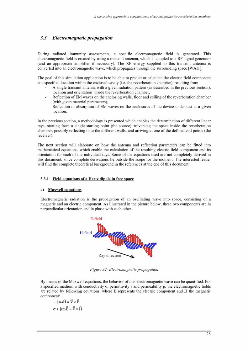
3.3.1 Field equations of a Hertz dipole in free space a) Maxwell equations Electromagnetic radiation is the propagation of an oscillating wave into space, consisting of a magnetic and an electric component. As illustrated in the picture below, these two components are in perpendicular orientation and in phase with each other.
E-field
H-field
Ray direction
Figure 32: Electromagnetic propagation
By means of the Maxwell equations, the behavior of this electromagnetic wave can be quantified. For a specified medium with conductivity σ, permittivity ε and permeability μ, the electromagnetic fields are related by following equations, where E represents the electric component and H the magnetic component:
EHjrrr
×∇=μω−
HEjrrr
×∇=εω+σ
28

A ray tracing approach to computational electromagnetics for reverberation chambers
29
b) Magnetic vector potential When deriving expressions for the magnetic and electric field components, often the magnetic vector potential A
r is introduced. This auxiliary function facilitates further theoretical elaboration. The
magnetic vector potential is a three dimensional vector field whose curl equals the magnetic field, which means that following expression holds:
AHrrr
×∇= It can be shown that, based on the latter expression and the Maxwell equation for the electric field component, E can also be formulated in terms of the magnetic vector potential:
( )[ ]AAj
1E 2 rrrrr•∇∇+γ−⋅
ωε+σ= with ( )εω+σμω=γ jj2
c) Hertz dipole
Now we consider an electric dipole source, which length is much smaller then the excited currents wavelength. Such a dipole is referred to as a Hertz dipole. Due to its infinitesimal length (λ<60), the current distribution may be considered to be distributed evenly along the dipole.
Figure 33: Current distribution assumption
Figure 34 shows a Hertz dipole I0dl, with length dl and applied current I0. It is oriented along the z axis in a Cartesian system.
Figure 34: Vector potential for a Hertz dipole
As mentioned earlier, our goal is to derive an equation for the electric field component at an arbitrary point P, caused by propagation from dipole I0dl. As a first step, we define the form of magnetic vector potential A
r. It has been proven in the literature that the vector potential for a Hertz dipole equals:
r.0 e.r4
dlIA γ−
π=
r
Also, the magnetic vector potential A is oriented parallel to the Hertz dipole, which is the Z axis in our example, independent from its position in space. This is due to the fact that the current which flows along the dipole has the same orientation as the dipole itself. For this reason it is indicated as vector Az in the figure above.
L I Current
distribution
P(x,y,z)
p
z
Y
Z
X
θ
Φ
I0dl
r
Az

A ray tracing approach to computational electromagnetics for reverberation chambers
30
We now know that the magnetic vector potential is only manifested in the same orientation as the Hertz dipole (the Z axis in our example), and we obtained an expression for Az which makes it quantifiable. Also, we initially stated that the magnetic vector potentials curl equals the magnetic field. Using this information in combination with the Maxwell equations allows us to derive following equations for Ex,y,z and Hx,y,z . Derivations are given in Appendix B.1.
=xHy
Az
∂∂
( ) =ωε+σ xEjzx
Az2
∂∂∂
=yHxAz
∂∂
− ( ) =ωε+σ yEjzy
Az2
∂∂∂
−
=zH 0 ( ) =ωε+σ zEj
2z2
2z2
yA
xA
∂
∂−
∂
∂−
Ez can alternatively be formulated by using the earlier proposed equation for Er
in terms of the magnetic vector potential, as illustrated in Appendix B.2:
⎥⎦⎤
⎢⎣⎡
∂∂+−⋅
+= 2
221
zAA
jE z
zz γωεσ
d) Spherical-polar coordinate system For computational considerations, it would be more convenient to use spherical-polar coordinates in stead of the Cartesian vector components to express the E
r and H
r field components. Within a
spherical-polar coordinate system, each vector in space is identified by three components (er, eθ and eΦ), as shown in Figure 35:
Figure 35: Vector decomposition for a spherical-polar coordinate system
It can be proven that, by converting the equations for Ex,y,z and Hx,y,z into spherical-polar components and substituting Az with its equation, following expressions are valid:
( ) θγ+⋅π
= γ−φ sin.e.r1
r4dl.IH r.
20
r
( ) ( ) θγ+⋅π
=ωε+σ γ− cos.e.r1r2dl.IEj r.
30
rr
( ) ( ) θγ+γ+⋅π
=ωε+σ γ−θ sin.e.rr1
r4dl.IEj r.22
30
r
This means that the electromagnetic propagation can be visualized by Figure 36, where
P
p
z Y
Z
X
θ
Φ
r
er
eΦ
eθ
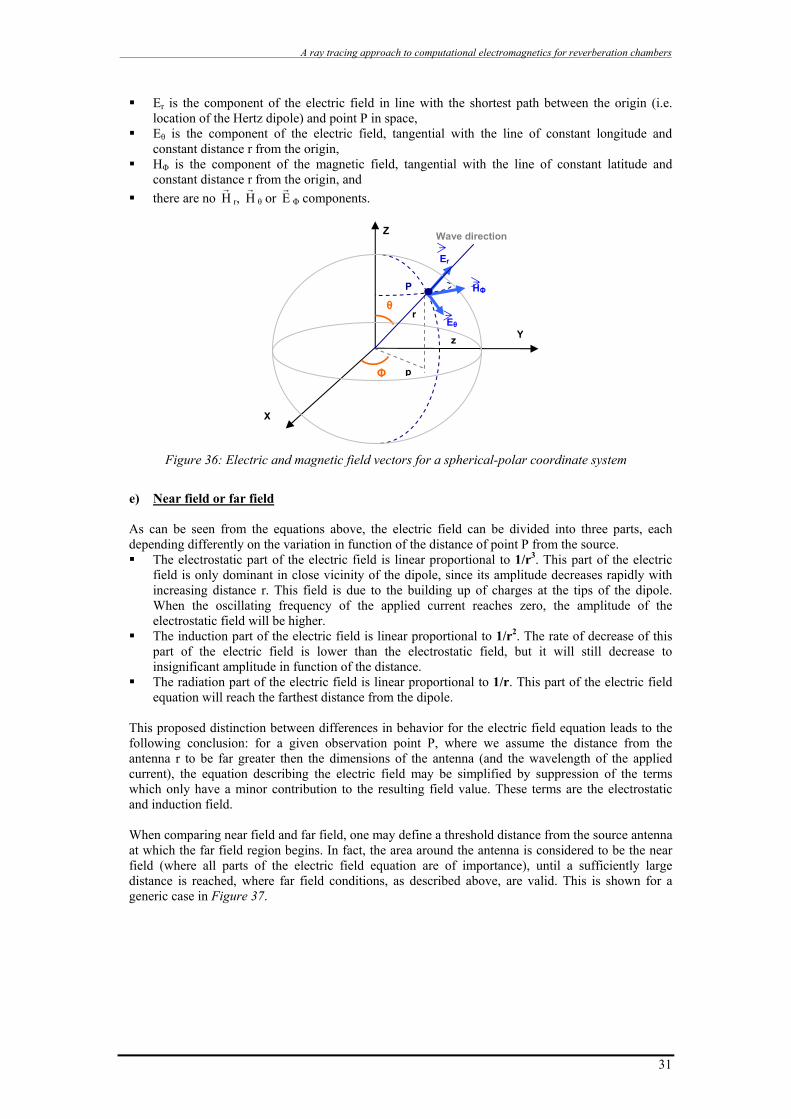
A ray tracing approach to computational electromagnetics for reverberation chambers
31
Er is the component of the electric field in line with the shortest path between the origin (i.e.
tial with the line of constant longitude and
tic field, tangential with the line of constant latitude and
location of the Hertz dipole) and point P in space, Eθ is the component of the electric field, tangen
constant distance r from the origin, HΦ is the component of the magne
constant distance r from the origin, and there are no H
rr, Hr
θ or ErΦ components.
Figure 36: Elec dinate system
e) Near field or far field
tric and magnetic field vectors for a spherical-polar coor
s can be seen from the equations above, the electric field can be divided into three parts, each
field is linear proportional to 1/r . The rate of decrease of this
ortional to 1/r. This part of the electric field
his proposed distinction between differences in behavior for the electric field equation leads to the
hen comparing near field and far field, one may define a threshold distance from the source antenna
Adepending differently on the variation in function of the distance of point P from the source. The electrostatic part of the electric field is linear proportional to 1/r3. This part of the electric
field is only dominant in close vicinity of the dipole, since its amplitude decreases rapidly with increasing distance r. This field is due to the building up of charges at the tips of the dipole. When the oscillating frequency of the applied current reaches zero, the amplitude of the electrostatic field will be higher.
The induction part of the electric 2
part of the electric field is lower than the electrostatic field, but it will still decrease to insignificant amplitude in function of the distance.
The radiation part of the electric field is linear propequation will reach the farthest distance from the dipole.
Tfollowing conclusion: for a given observation point P, where we assume the distance from the antenna r to be far greater then the dimensions of the antenna (and the wavelength of the applied current), the equation describing the electric field may be simplified by suppression of the terms which only have a minor contribution to the resulting field value. These terms are the electrostatic and induction field. Wat which the far field region begins. In fact, the area around the antenna is considered to be the near field (where all parts of the electric field equation are of importance), until a sufficiently large distance is reached, where far field conditions, as described above, are valid. This is shown for a generic case in Figure 37.
P
p
z Y
Z
X
θ
Φ
r
HΦ
Eθ
Wave direction
Er
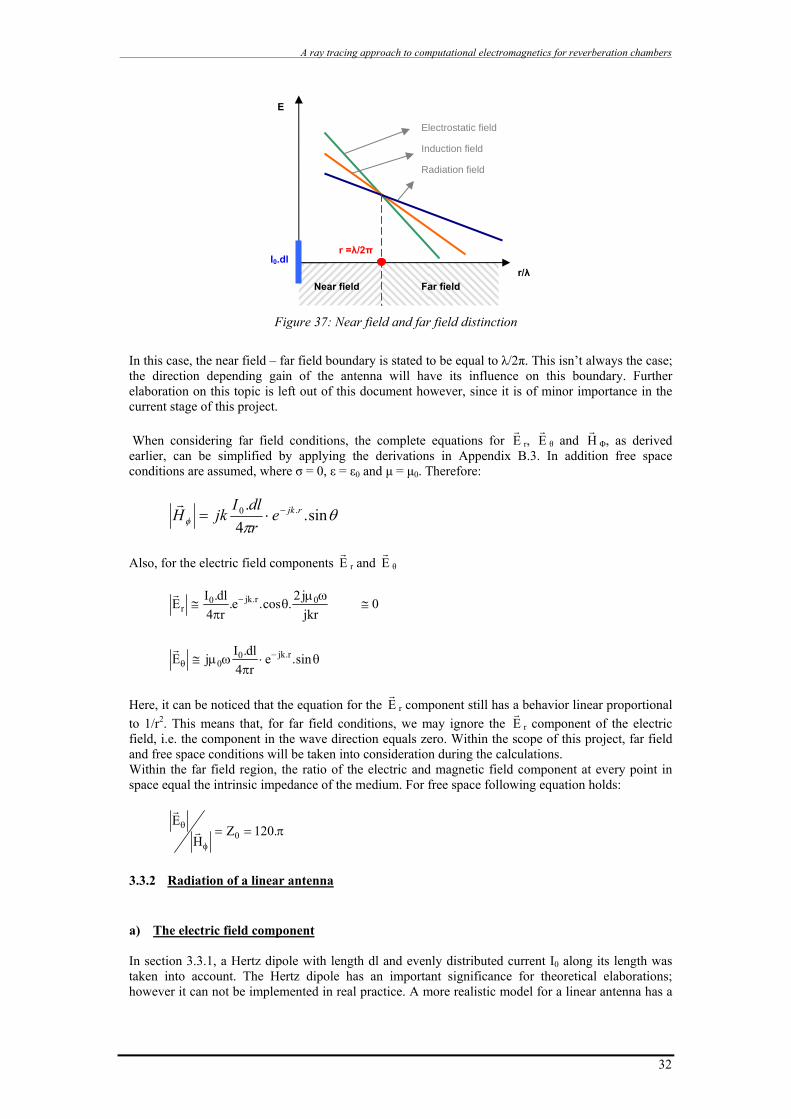
A ray tracing approach to computational electromagnetics for reverberation chambers
E
Electrostatic field
Induction field
Radiation field
r =λ/2π
Figure 37: Near field and far field distinction
In this case, the near field – far field boundary is stated to be equal to λ/2π. This isn’t always the case; the direction depending gain of the antenna will have its influence on this boundary. Further elaboration on this topic is left out of this document however, since it is of minor importance in the current stage of this project. When considering far field conditions, the complete equations for E
rr, E
rθ and Φ, as derived
earlier, can be simplified by applying the derivations in Appendix B.3. In addition free space conditions are assumed, where σ = 0, ε = ε0 and μ = μ0. Therefore:
Hr
θπφ sin.
4. .0 rjkerdlI
jkH −⋅=r
Also, for the electric field components E
rr and E
rθ
jkrj2.cos.e.
r4dl.IE 0r.jk0
rωμ
θπ
≅ −r 0≅
θ⋅π
ωμ≅ −θ sin.e
r4dl.IjE r.jk0
0r
Here, it can be noticed that the equation for the E
rr component still has a behavior linear proportional
to 1/r2. This means that, for far field conditions, we may ignore the Er
r component of the electric field, i.e. the component in the wave direction equals zero. Within the scope of this project, far field and free space conditions will be taken into consideration during the calculations. Within the far field region, the ratio of the electric and magnetic field component at every point in space equal the intrinsic impedance of the medium. For free space following equation holds:
π==φ
θ .120ZH
E0r
r
3.3.2 Radiation of a linear antenna a) The electric field component In section 3.3.1, a Hertz dipole with length dl and evenly distributed current I0 along its length was taken into account. The Hertz dipole has an important significance for theoretical elaborations; however it can not be implemented in real practice. A more realistic model for a linear antenna has a
r/λ Near field
I0.dl
Far field
32
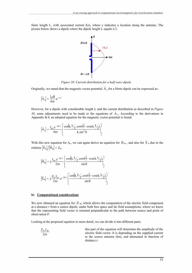
A ray tracing approach to computational electromagnetics for reverberation chambers
finite length L, with associated current I(z), where z indicates a location along the antenna. The picture below shows a dipole where the dipole length L equals λ/2.
Z
Z=L/2
| Im |
Z= - L/2
I(z)
Figure 38: Current distribution for a half wave dipole
Originally, we stated that the magnetic vector potential Ar
z for a Hertz dipole can be expressed as:
r.0z e.
r4dlIA γ−
π=
r
However, for a dipole with considerable length L and the current distribution as described in Figure 38, some adjustments need to be made to the equations of A
rz. According to the derivations in
Appendix B.4, an adopted equation for the magnetic vector potential is found:
( )⎥⎥
⎦
⎤
⎢⎢
⎣
⎡
θ
−θ
π=
−
2
r.k.jm
z sin.k
)2L.kcos(cos.2
L.kcos.
r4e.IA
r
With this new equation for Az, we can again derive an equation for H
rΦ , and also for E
rθ due to the
relation 0ZHE =φθ
rr.
( )
⎥⎥
⎦
⎤
⎢⎢
⎣
⎡
θ
−θ
π=
−
φ sin
)2L.kcos(cos.2
L.kcos.
r2e.I.jH
r.k.jm
r
( )
⎥⎥
⎦
⎤
⎢⎢
⎣
⎡
θ
−θ
π= −
θ sin
)2L.kcos(cos.2
L.kcos.e.
r2I.Z.jE r.k.jm0
r
b) Computational considerations We now obtained an equation for | E θ|, which allows the computation of the electric field component at a distance r from a source dipole, under both free space and far field assumptions, where we know that the representing field vector is oriented perpendicular to the path between source and point of observation P.
r
Looking at the proposed equation in more detail, we can divide it into different parts.
r2I.Z m0
π
this part of the equation will determine the amplitude of the electric field vector. It is depending on the supplied current to the source antenna (Im), and attenuated in function of distance r.
33

A ray tracing approach to computational electromagnetics for reverberation chambers
r.k.je.j − The complex part of the equation provides information concerning the phase of the electric field vector in function of r.
( )⎥⎥
⎦
⎤
⎢⎢
⎣
⎡
θ
−θ
sin
)2L.kcos(cos.2
L.kcos
The third part of the equation specifies the radiation field pattern. The amount of energy transmitted from the antenna is dependent from the azimuth angle θ, and is therefore referred to as F(θ).
F(θ) is a known function with low complexity for a dipole. For a half wave dipole, this F(θ) pattern is illustrated in Figure 15.Knowing θ, it is possible to derive F(θ), which has an amplitude within interval [0,1]. It can therefore be stated that F(θ) will as well determine the resulting amplitude of the electric field vector. In real practice, tuned dipoles are rarely used for broadband applications, because they are specifically designed to attain optimal radiation for a limited amount of discrete frequencies (nλ/2). Other more common antennas are e.g. biconical, log periodic and horn antennas. Within the scope of this project , the disadvantage for the simulation application when choosing these more appropriate antenna types is that their radiation pattern is rarely given as a function of θ. An adequate solution therefore needs to be worked out in order to obtain realistic results for F(θ). A possible scenario may be to measure the radiation pattern of the chosen antenna. This can be done using a closed loop measurement, where the radiated field at a specified distance is measured at different angles (azimuth and elevation). More details about these measurements are available, but lie outside the scope of this project. For certain types of antennas, simulation application, specifically developed to simulate the radiation pattern of an antenna, may be applied. Until now, we conclude that we have the means to calculate the electric field vector at a given point of observation, following a specific direct path (i.e. without reflection) starting from the source antenna as, given the following parameters: Location of the source antenna and its orientation, Location of point of observation P (distance r and angle θ) , Radiation pattern of the source antenna,
and assuming free space and far field conditions. Now, what about the influence of reflection of wave paths against the walls and mode stirrer panels? This question still remains to be answered, and is dealt with in the section 3.3.3.
3.3.3 Reflection of electromagnetic waves a) Spectral reflection Within the scope of this project, we consider reflection of electromagnetic waves on smooth surfaces with high conductivity. Assuming a smooth surface (with size of irregularities < λ/(16.sinψ), where ψ is the grazing angle of incidence), only spectral reflection may be taken into account. This means that the angle of the reflected wave path θr is equal to the angle of the incident wave path θi, with respect to the normal N of the surface. Possible diffuse reflection or scattering is assumed to be negligible.
R
I N
ψ
Өi Өr
T
Figure 39: Spectral reflection
34
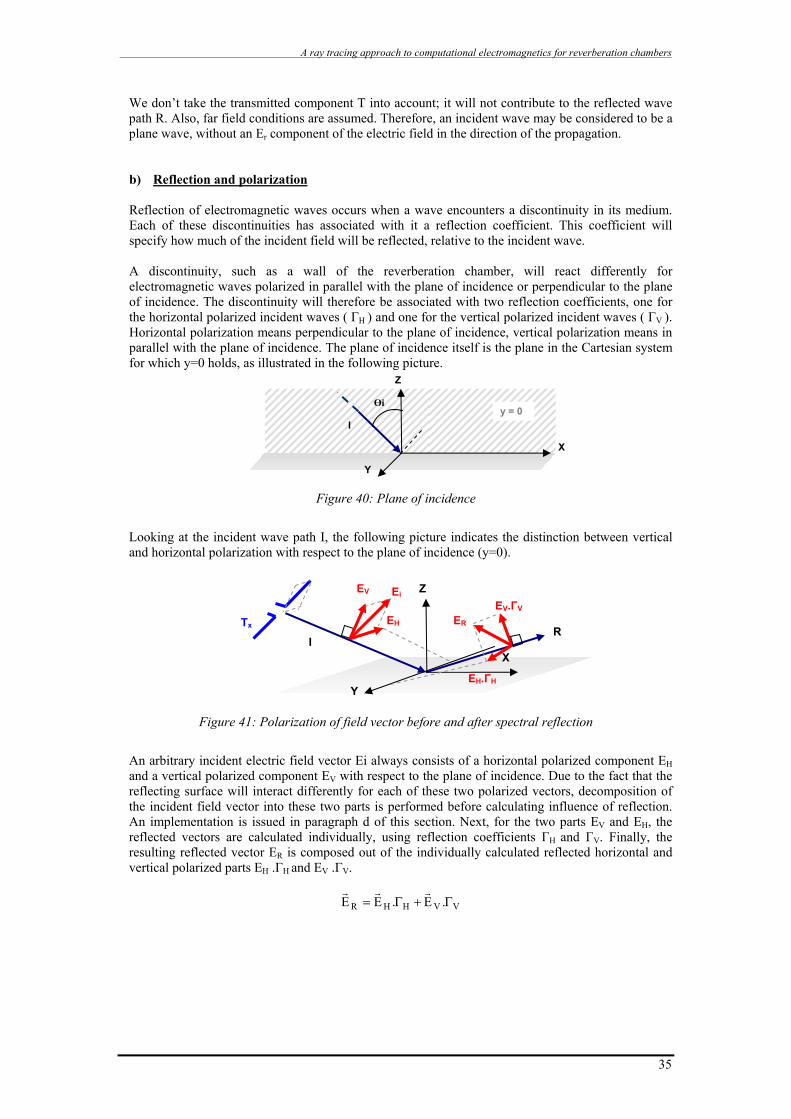
A ray tracing approach to computational electromagnetics for reverberation chambers
We don’t take the transmitted component T into account; it will not contribute to the reflected wave path R. Also, far field conditions are assumed. Therefore, an incident wave may be considered to be a plane wave, without an Er component of the electric field in the direction of the propagation. b) Reflection and polarization Reflection of electromagnetic waves occurs when a wave encounters a discontinuity in its medium. Each of these discontinuities has associated with it a reflection coefficient. This coefficient will specify how much of the incident field will be reflected, relative to the incident wave. A discontinuity, such as a wall of the reverberation chamber, will react differently for electromagnetic waves polarized in parallel with the plane of incidence or perpendicular to the plane of incidence. The discontinuity will therefore be associated with two reflection coefficients, one for the horizontal polarized incident waves ( ΓH ) and one for the vertical polarized incident waves ( ΓV ). Horizontal polarization means perpendicular to the plane of incidence, vertical polarization means in parallel with the plane of incidence. The plane of incidence itself is the plane in the Cartesian system for which y=0 holds, as illustrated in the following picture.
Z
Y
I
Өi y = 0
X
Figure 40: Plane of incidence
Looking at the incident wave path I, the following picture indicates the distinction between vertical and horizontal polarization with respect to the plane of incidence (y=0).
Z
X I
Y
EV
EH
Ei
R ER
EV.ΓV
EH.ΓH
Tx
Figure 41: Polarization of field vector before and after spectral reflection
An arbitrary incident electric field vector Ei always consists of a horizontal polarized component EH and a vertical polarized component EV with respect to the plane of incidence. Due to the fact that the reflecting surface will interact differently for each of these two polarized vectors, decomposition of the incident field vector into these two parts is performed before calculating influence of reflection. An implementation is issued in paragraph d of this section. Next, for the two parts EV and EH, the reflected vectors are calculated individually, using reflection coefficients ΓH and ΓV. Finally, the resulting reflected vector ER is composed out of the individually calculated reflected horizontal and vertical polarized parts EH .ΓH and EV .ΓV.
VVHHR .E.EE Γ+Γ=rrr
35

A ray tracing approach to computational electromagnetics for reverberation chambers
c) Reflection coefficients The reflection coefficients define how much energy from the incident wave will be reflected. The concept of a horizontal and vertical reflection coefficient has already been introduced. What remains are equations which allow quantification of Γh and Γv. From a theoretical approach, where we assume a reflecting smooth surface of infinite dimensions, reflection coefficient equations, relating the reflected vector to the incident vector, are defined by Fresnel:
θ−+θ
θ−−θ=Γ
22d
22d
HsinNcos
sinNcos
θ−+θ
θ−−θ=Γ
22d
2d
22d
2d
VsinNcosN
sinNcosN
where θ denotes the angle of incidence, and Nd the refractive index 0dN εε= (depending on the material parameters). For a perfect conducting material, Nd >> 1. Therefore, ΓH and ΓV approach the following values, independent from θ:
1H −=Γ and 1V =Γ
Implementing these coefficients mean that we assume a lossless reflection. This is a theoretical assumption; however the materials used inside a reverberation chamber (aluminum plates), are specifically chosen to have a very high reflection. Therefore, the assumption of perfectly conducting material is acceptable as a first approach. These ‘simplified’ coefficients mean that for horizontal polarization, the orientation of the reflected field vector will be inversed with respect to the horizontal polarized incident field vector, as can bee seen in the picture above. The orientation of the vertical polarized field vector remains identical with respect to the wave path. However, due to the fact that the wave path itself is reoriented after reflection, the resulting orientation of the EV vector changes as well and needs to be calculated. This is discussed in the next section. d) Implementation of vector decomposition and vector reorientation after reflection
Taking the conclusion of the previous section into account, the following pictures show how the reflected field vectors behave for horizontal and vertical polarizations with respect to the plane of incidence separately.
Z
X
EH
Ei
R
EH.ΓH
EH EH.ΓH
I
Y
Figure 42: Horizontal component of field vector before and after reflection
36

A ray tracing approach to computational electromagnetics for reverberation chambers
37
Figure 43: Vertical component of field vector before and after reflection
It was stated that the resulting reflected field vector RE
rcan be calculated as follows:
VVHHR .E.EE Γ+Γ=rrr
However, the pictures show us clearly that there is a reorientation between both vertical components of the incident, respectively reflected field vector. This leads to the idea that some vector calculus will be needed. We first start by introducing unit vectors h
r and ivr , where h
r acts as unit vector in the direction of
the horizontal polarized component of the electric vector field, ivr for the vertical polarized component of the incident ray path (see next figure). These unit vectors allow us to rewrite the latter expression as follows:
RVVHHR v..Eh..EE rrrrrΓ+Γ=
Figure 44: Horizontal unit vector
Figure 45: Vertical unit vector
Z
X
Y
EH R
EH.ΓH
EH EH.ΓH
I ur
ur−
Z
X Y
EV
R
EV.ΓV EV I
EV.ΓV
ivrRvr
Z
X
Y
EV
Ei
R
EVR.ΓV EV
I EV.ΓV

A ray tracing approach to computational electromagnetics for reverberation chambers
38
The unit vectors can be found by applying the following equations: nuh irrr
×= and ii uhv rrr×=
where iur is the unit vector of the incident ray. As a next step, we need to obtain HE
r and VE
r, i.e. the two field vector components’ amplitudes.
These values van be calculated by applying:
hEE iHrrr
•=
hEE HHrrr
•=⇒
HiV EEErrr
−=⇒
VEr
⇒ can be calculated
The reason why we can’t simply use HE
r and VE
rin the initial equation is that we also need to
consider the vector reorientation (due to the reflection). This reorientation is calculated by using the unit vectors h
r and ivr . The horizontal unit vector h
r remains the same after reflection. The vertical
unit vector ivr however will be reoriented. I.e. a new unit vector Rvr will appear. The equation below allows quick calculation of Rvr , using iur , ivr and n
r, the surface normal:
( ) ( )( )( )hn.vhnn.vnv iiR
rrrrrrrrrו×−•=
The equation for Rvr can be visualized by the following picture:
Figure 46: Determination of vertical field component after reflection by vector calculus
We now have calculated all the necessary components to allow calculation of field vector . RE
r
e) Phase difference between reflected and direct path
For a perfect conducting material, physics shows that excess charges will optimally distance themselves along the conducting material in order to reach electrostatic equilibrium. For this reason, the component of the incident electric field vector, parallel to the coincided plane, is shifted 180 degrees in phase with respect to the incident field vector. This way, the electrostatic charge at the location of the intersection is zero. This phase shift has been accounted for in the calculations of the reflected field vector, as was discussed in the previous section.
N
X
ivrRvr
( )n.vn irrr
•
( )( )( )hn.vhn irrrrr
ו×−
hr
iur
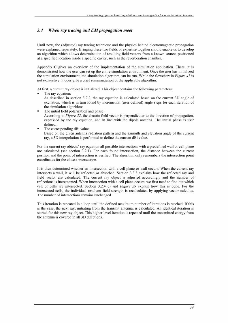
A ray tracing approach to computational electromagnetics for reverberation chambers
3.4 When ray tracing and EM propagation meet
Until now, the (adjusted) ray tracing technique and the physics behind electromagnetic propagation were explained separately. Bringing these two fields of expertise together should enable us to develop an algorithm which allows determination of resulting field vectors from a known source, positioned at a specified location inside a specific cavity, such as the reverberation chamber. Appendix C gives an overview of the implementation of the simulation application. There, it is demonstrated how the user can set up the entire simulation environment. Once the user has initialized the simulation environment, the simulation algorithm can be run. While the flowchart in Figure 47 is not exhaustive, it does give a brief summarization of the applicable algorithm. At first, a current ray object is initialized. This object contains the following parameters: The ray equation:
As described in section 3.2.2, the ray equation is calculated based on the current 3D angle of excitation, which is in turn found by incremental (user defined) angle steps for each iteration of the simulation algorithm:
The initial field polarization and phase: According to Figure 32, the electric field vector is perpendicular to the direction of propagation, expressed by the ray equation, and in line with the dipole antenna. The initial phase is user defined.
The corresponding dBi value: Based on the given antenna radiation pattern and the azimuth and elevation angle of the current ray, a 3D interpolation is performed to define the current dBi value.
For the current ray objects’ ray equation all possible intersections with a predefined wall or cell plane are calculated (see section 3.2.1). For each found intersection, the distance between the current position and the point of intersection is verified. The algorithm only remembers the intersection point coordinates for the closest intersection. It is then determined whether an intersection with a cell plane or wall occurs. When the current ray intersects a wall, it will be reflected or absorbed. Section 3.3.3 explains how the reflected ray and field vector are calculated. The current ray object is adjusted accordingly and the number of reflections is incremented. When intersection with a cell plane occurs, we first need to find out which cell or cells are intersected. Section 3.2.4 c) and Figure 29 explain how this is done. For the intersected cells, the individual resultant field strength is recalculated by applying vector calculus. The number of intersections remains unchanged. This iteration is repeated in a loop until the defined maximum number of iterations is reached. If this is the case, the next ray, initiating from the transmit antenna, is calculated. An identical iteration is started for this new ray object. This higher level iteration is repeated until the transmitted energy from the antenna is covered in all 3D directions.
39
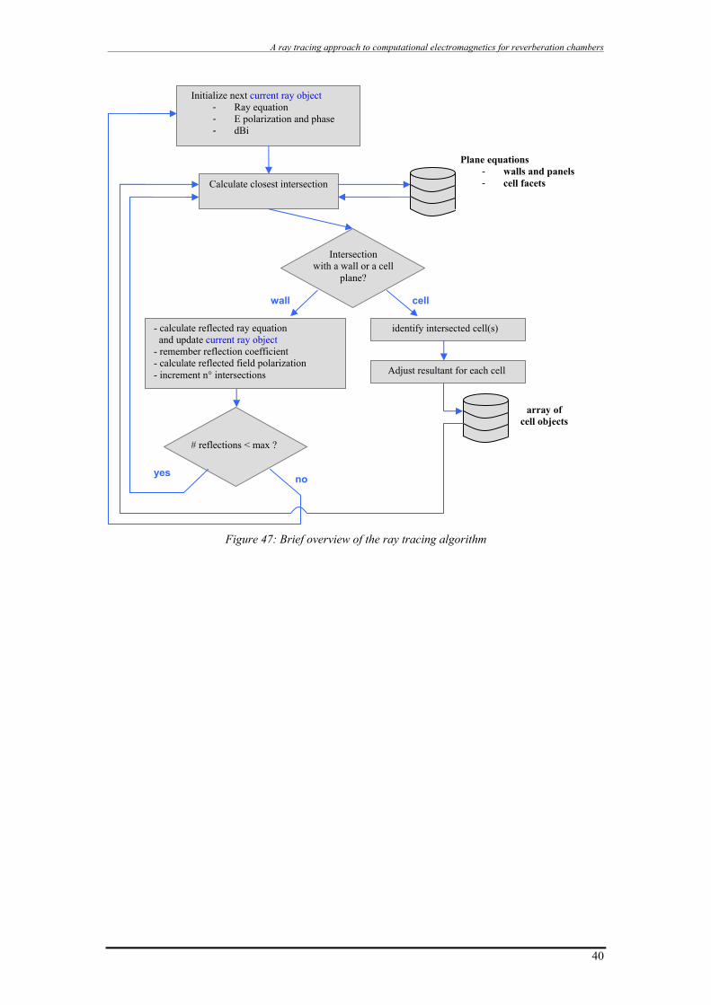
A ray tracing approach to computational electromagnetics for reverberation chambers
Initialize next current ray object - Ray equation - E polarization and phase - dBi
Intersection with a wall or a cell
plane?
wall
- calculate reflected ray equation and update current ray object - remember reflection coefficient - calculate reflected field polarization - increment n° intersections
Calculate closest intersection
Plane equations - walls and panels - cell facets
cell
# reflections < max ?
yes no
identify intersected cell(s)
array of cell objects
Adjust resultant for each cell
Figure 47: Brief overview of the ray tracing algorithm
40
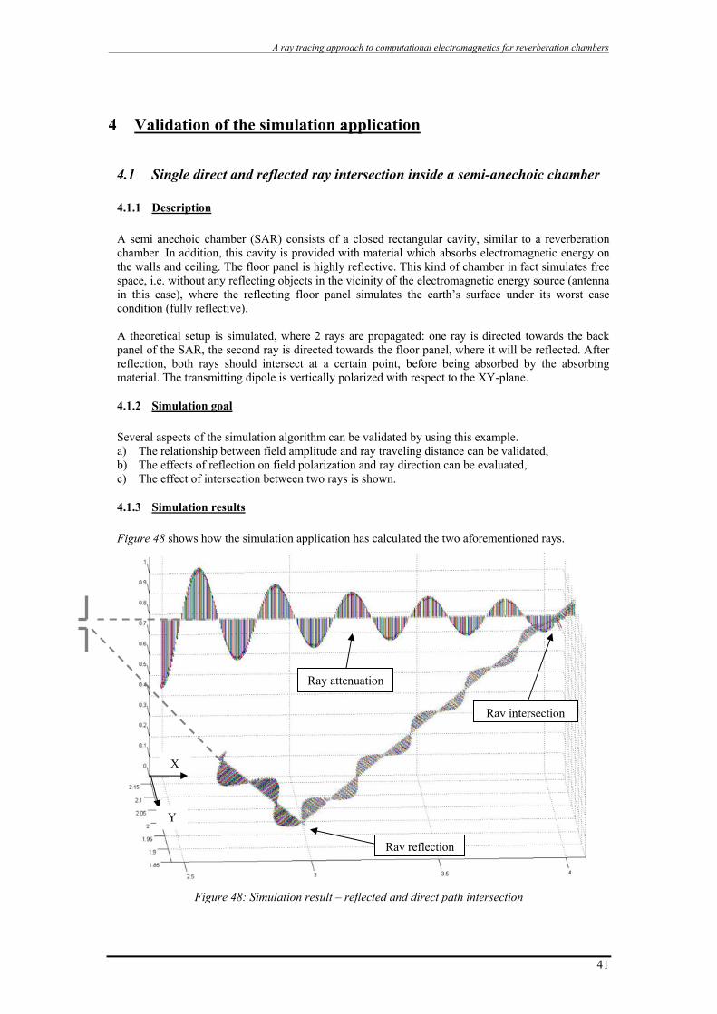
A ray tracing approach to computational electromagnetics for reverberation chambers
4 Validation of the simulation application
4.1 Single direct and reflected ray intersection inside a semi-anechoic chamber
4.1.1 Description
A semi anechoic chamber (SAR) consists of a closed rectangular cavity, similar to a reverberation chamber. In addition, this cavity is provided with material which absorbs electromagnetic energy on the walls and ceiling. The floor panel is highly reflective. This kind of chamber in fact simulates free space, i.e. without any reflecting objects in the vicinity of the electromagnetic energy source (antenna in this case), where the reflecting floor panel simulates the earth’s surface under its worst case condition (fully reflective).
A theoretical setup is simulated, where 2 rays are propagated: one ray is directed towards the back panel of the SAR, the second ray is directed towards the floor panel, where it will be reflected. After reflection, both rays should intersect at a certain point, before being absorbed by the absorbing material. The transmitting dipole is vertically polarized with respect to the XY-plane.
4.1.2 Simulation goal
Several aspects of the simulation algorithm can be validated by using this example. a) The relationship between field amplitude and ray traveling distance can be validated, b) The effects of reflection on field polarization and ray direction can be evaluated, c) The effect of intersection between two rays is shown.
4.1.3 Simulation results
Figure 48 shows how the simulation application has calculated the two aforementioned rays.
Figure 48: Simulation result – reflected and direct path intersection
X
Ray attenuation
Ray intersection
Y
Ray reflection
41

A ray tracing approach to computational electromagnetics for reverberation chambers
For this example, it was chosen to represent the simulated field strength by a vector field. The result shown in Figure 48 is a composition of the results of 9 successive simulations. This was needed since no more than 275000 cells could be used for each simulation. Most of the cells were never reached by a ray however.
Ray attenuation
The resulting field strength is calculated by the applying the derived formula for | θ |, as mentioned in section
Er
3.3.2. This means that the amplitude relates to 1/r, with r the distance from the antenna. Figure 48 indeed shows the result of field strength calculation according to this formula for both rays. This is indicated in Figure 49.
Figure 49: Simulation result – ray attenuation evaluation
Ray reflection As was discussed in section 3.3.3, when ray reflection on a surface occurs, the reflected component may be (partially) absorbed. The reflection coefficient, associated with the intersected panel, is used to define the reflection (and therefore also the absorption) rate. A second consequence of reflection is the effect on the field polarization. Vector components which are reciprocal to the incident plane will keep the same orientation after reflection, vector components which are parallel to the incident plane will be reflected in the opposite orientation.
Figure 50: Simulation result – ray reflection evaluation
Figure 50 shows how reflection is calculated for the given simulation project. Figure 51 shows a close-up of the point of intersection, where only the last calculated field vector before incidence, and the first field vector after reflection are shown. The vector values are shown in the table below.
( )⎥⎥
⎦
⎤
⎢⎢
⎣
⎡
θ
−θ
π= −
θ sin
)2L.kcos(cos.2
L.kcos.e.
r2I.Z
.jE r.k.jm0r
Point of reflection
42

A ray tracing approach to computational electromagnetics for reverberation chambers
Before reflection
Unit vectors before reflection
After reflection
Unit vectors after reflection
x-comp. -6,609312241 -1 5,424178296 1 y-comp. 0 0 0 0 z-comp. -6,609312241 -1 5,424178296 1
The derived unit vectors for both rays show that the reorientation of the field vector due to reflection indeed complies with the described procedure in section 3.3.3, where the unit vector, reciprocal to the intersected plane, keeps its orientation and the unit vector parallel to the intersected plane is inverted.
Although for this example the reflection coefficient of the bottom plane equals 1, the amplitudes of both rays are different. The reason for this is that the field vector component after reflection is calculated for a point on the ray (b in Figure 51) which lies a little bit farther than the point on the ray where the vector component before reflection is calculated (a in Figure 51), resulting in a slight attenuation. A second reason is that, due to this distance, there exists a phase difference between point a and b.
a b Ray path
Figure 51: Simulation result – close-up of ray reflection
Ray intersection
Figure 52 gives a close-up of the intersection point between both rays. The resulting field vectors at the point of intersection are the result of a vector summation between the individual field vectors of both rays. Exact values for these field vectors are given in the table below.
Figure 52: Simulation result – ray intersection evaluation
Vector before reflection
Vector after reflection
Point of reflection (3,2,0)
Point of intersection
43
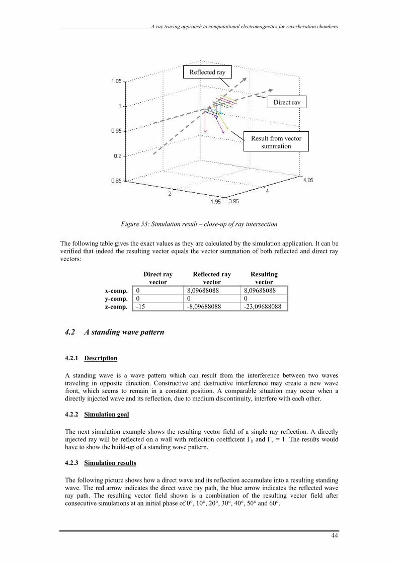
A ray tracing approach to computational electromagnetics for reverberation chambers
Figure 53: Simulation result – close-up of ray intersection
The following table gives the exact values as they are calculated by the simulation application. It can be verified that indeed the resulting vector equals the vector summation of both reflected and direct ray vectors:
Direct ray
vector Reflected ray
vector Resulting
vector x-comp. 0 8,09688088 8,09688088 y-comp. 0 0 0 z-comp. -15 -8,09688088 -23,09688088
4.2 A standing wave pattern
4.2.1 Description
A standing wave is a wave pattern which can result from the interference between two waves traveling in opposite direction. Constructive and destructive interference may create a new wave front, which seems to remain in a constant position. A comparable situation may occur when a directly injected wave and its reflection, due to medium discontinuity, interfere with each other.
4.2.2 Simulation goal
The next simulation example shows the resulting vector field of a single ray reflection. A directly injected ray will be reflected on a wall with reflection coefficient Гh and Гv = 1. The results would have to show the build-up of a standing wave pattern.
4.2.3 Simulation results
The following picture shows how a direct wave and its reflection accumulate into a resulting standing wave. The red arrow indicates the direct wave ray path, the blue arrow indicates the reflected wave ray path. The resulting vector field shown is a combination of the resulting vector field after consecutive simulations at an initial phase of 0°, 10°, 20°, 30°, 40°, 50° and 60°.
Reflected ray
Direct ray
Result from vector summation
44

A ray tracing approach to computational electromagnetics for reverberation chambers
Resultant at different phase angles
Wall reflection point
Figure 54: Simulation result – Standing wave pattern
Figure 55 shows the same situation from another viewpoint. In this figure, both reflected and direct waves are shown separately as the red, respectively blue vector field. This example clearly shows the 180° phase shift after reflection. Addition of both vector fields results in a standing wave pattern (shown in green in Figure 55), as was illustrated in Figure 54 for different other initial phases.
Resultant
Figure 55: Simulation result – direct and reflected wave decomposition
The general behavior indeed corresponds to the theoretically expected wave pattern. Inaccuracies are present however, which may be explained by the fact that there exists a certain resolution in the calculations, which depends on the individual cell size and the locations where the direct and reflected wave intersect with these cells. This is shown in Figure 56: where the resulting vector field shows a single resultant vector, located at each individual cells’ reference location (the center of the cube), this resultant value is calculated as the sum of the amplitude of the direct ray at location a, and the amplitude of the reflected ray at location b, which differ from each other. This leads to some inaccuracy in the resulting vector field.
reflected
direct
45
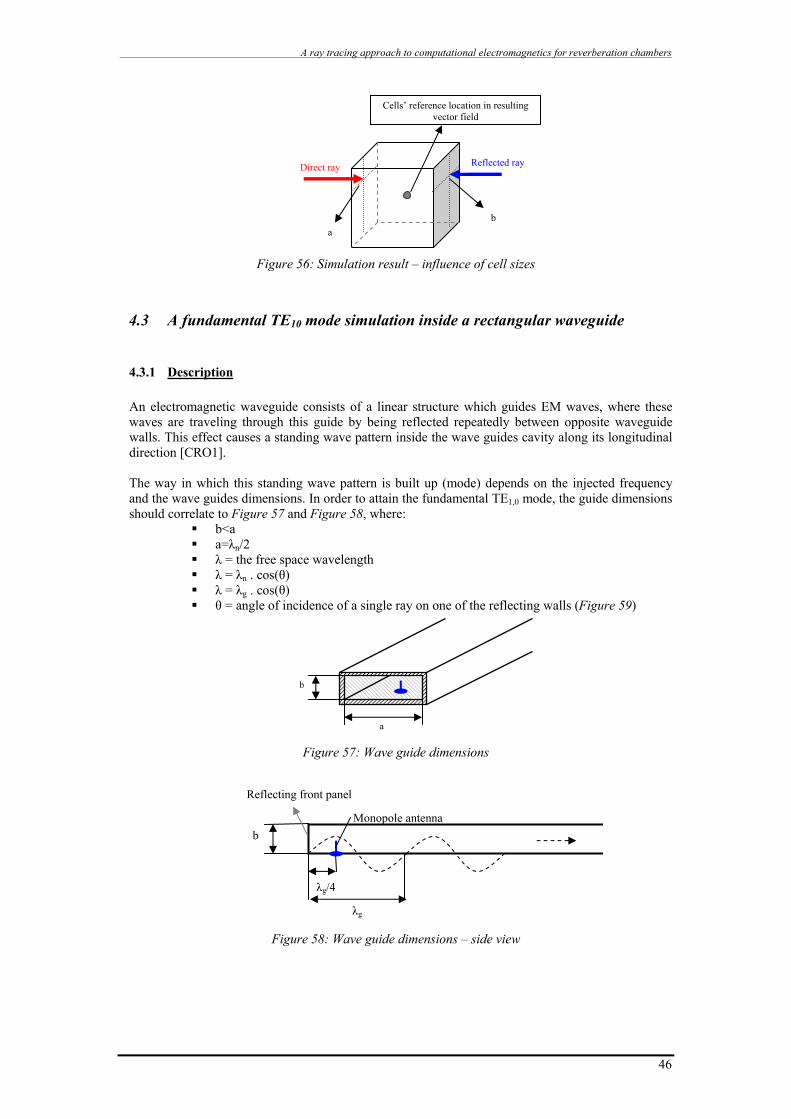
A ray tracing approach to computational electromagnetics for reverberation chambers
Cells’ reference location in resulting vector field
Reflected ray Direct ray
b a
Figure 56: Simulation result – influence of cell sizes
4.3 A fundamental TE10 mode simulation inside a rectangular waveguide
4.3.1 Description
An electromagnetic waveguide consists of a linear structure which guides EM waves, where these waves are traveling through this guide by being reflected repeatedly between opposite waveguide walls. This effect causes a standing wave pattern inside the wave guides cavity along its longitudinal direction [CRO1].
The way in which this standing wave pattern is built up (mode) depends on the injected frequency and the wave guides dimensions. In order to attain the fundamental TE1,0 mode, the guide dimensions should correlate to Figure 57 and Figure 58, where:
b<a a=λn/2 λ = the free space wavelength λ = λn . cos(θ) λ = λg . cos(θ) θ = angle of incidence of a single ray on one of the reflecting walls (Figure 59)
b
a
Figure 57: Wave guide dimensions
Reflecting front panel
Monopole antenna
Figure 58: Wave guide dimensions – side view
b
λg/4
λg
46

A ray tracing approach to computational electromagnetics for reverberation chambers
Figure 59: internal angle of incidence
4.3.2 Simulation goal
One could calculate the exact behavior of the propagated electromagnetic field inside a waveguide by applying Maxwell’s equations. These calculations are very tedious however. For this reason, this analysis will mainly focus on the general behavior of the simulated field, where for example a standing wave pattern should appear for a simulated TE1,0 setup.
4.3.3 Simulation results
Figure 60 shows the resulting field strength inside a waveguide with dimensions a = 0.15m and b = 0.05m, over a length of 1m. A monopole antenna is used as a source antenna, where the source frequency is set at 1GHz (λ ≈ 0.3m) and initial phase at 0°. The monopole antenna is located at a distance of 0.075m (λ/4, and not λg/4 since θ varies for each single ray!) from the reflecting front panel, in the center of the wave guides width. While the simulation application delivers a 3D vector field, Figure 60 only shows the amplitude of the vertical polarized component of each field vector. Secondly, the results are shown for each cell with an identical z-index, which means that only a horizontal slice from the resulting vector field is shown. This way of partially visualizing the vector field gives a clearer view of a part of the complete data set.
Figure 60: simulation result of a wave guide TE1,0 mode
Theoretical and behavioral expectation
As already mentioned, it is to be expected that a standing wave pattern is built up inside the waveguide cavity. From the simulation results, we can indeed distinguish a kind of standing wave distribution along the waveguide’s longitudinal axis. This can be seen more clearly when taking a side view representation of the simulation data, as in Figure 61.
λg/2 a
θ θ Ray 1
λg Ray 2
λn θ
47

A ray tracing approach to computational electromagnetics for reverberation chambers
Figure 61: simulation result of a wave guide TE1,0 mode- side view
It needs to be verified however if indeed this standing wave complies with the theoretical behavior. Some important remarks can be made in advance, which emphasize some differences in the approach to this problem between a theoretical model and the model calculated by simulation. As has been explained in the previous section, in theory a wavelength λg for the standing wave
pattern along the axis of the waveguide can be calculated, based on the angle of incidence θ of a specific ray (Figure 59). Considering the calculations made by the simulation application, this angle θ will vary with each single ray. Therefore, λg can not be calculated as a single value, but it will have a value within certain boundaries.
Most theoretical models only take into account those rays which lie within the horizontal XY-plane. This simulation uses a 3D approach, where each cell will be intersected not only by rays propagated on the horizontal plane, but also by rays which have been reflected on the top or bottom wall of the waveguide for example.
Taking these remarks into account, and looking back at the simulation results from above (top view), we get Figure 62. This top view represents the calculated field values in function of the cell positions along the length and width of the waveguide. Each cell’s resultant field magnitude (the vertical component of the simulated field strength) is represented by a color. Red represents a high positive field strength, green-yellow an intermediary value (near zero) and blue a negative field strength.
Length
Monopole Figure 62: simulation result of a wave guide TE1,0 mode- top view
A standing wave pattern throughout the length of the waveguide is indeed present in the simulation results. The initial part however, near the transmitting monopole antenna, behaves rather particularly. Some abrupt changes in the field strength and polarization are noticeable. These values may find their reason in the fact that for all field strength calculations, a far field approximation is used. Near the transmit antenna, near field calculations should be used if accurate results are wanted. The decision to rely on far field approximations only was made and discussed in section 3.3.1 part e).
Further investigation on how the resultant values are found would mean that for the entire simulation on would backtrack each ray. For the results shown, each simulation run used approximately 260000 rays (0.5° angle step size) for a total of 3375 cells (15x15x15 cells). The entire dataset as shown in Figure 60, Figure 61 and Figure 62 is the result of 8 test runs. Based on the previous test case (and many similar ones), it is assumed that the simulation application behaves according to its theoretical description in Chapter 3.
48

A ray tracing approach to computational electromagnetics for reverberation chambers
Inaccuracy by limited number of reflections
As was mentioned earlier in this conclusion, the maximum number of reflections is limited. This aspect leads to the following inaccuracy consideration, where angles Ө1 and Ө2 can be calculated as an approximation of the limited range of the rays:
In the given example, the source antenna (monopole) is located at a distance x1 from the reflecting front panel. Assuming the number of reflections equals 10, we can determine a group of initial rays (starting at the source antenna), which will never reach a defined cell group. For example:
Figure 63: Ray contribution inside waveguide, Ө1
The example shows one initial ray (blue), which encountered 10 reflections on its path. After the 10th reflection, the next ray will be considered. Since this blue ray never reached the cell group, it will not contribute to the final result. Based on this example, angle Ө1 can be determined in case x1 is known: )
5,9(
11 x
aarctg=θ
Similarly, not all rays propagated in the direction of the cell group will contribute to the final result. The following figure should illustrate this. Here, x2 represents the distance between the source antenna and the first cell plane of the cell group. For this example, angle Ө2 can be calculated as follows: )
5,9(
22 x
aarctg=θ
Figure 64: ray contribution inside waveguide, Ө2
4.4 Effects of an aperture inside a rectangular waveguide
4.4.1 Description
We reconsider the waveguide from the previous example. An additional panel is inserted inside the cavity of the waveguide, in parallel with the front panel. This additional panel is provided with a narrow aperture, where the aperture width is smaller then the injected wavelength λ. In theory, this aperture should block transmission through the waveguide beyond the additional panel.
Source antenna
X Cell group
x2
a
Ө2
a/2
Source antenna
X
Ө1
aCell group
a/2
x1
49
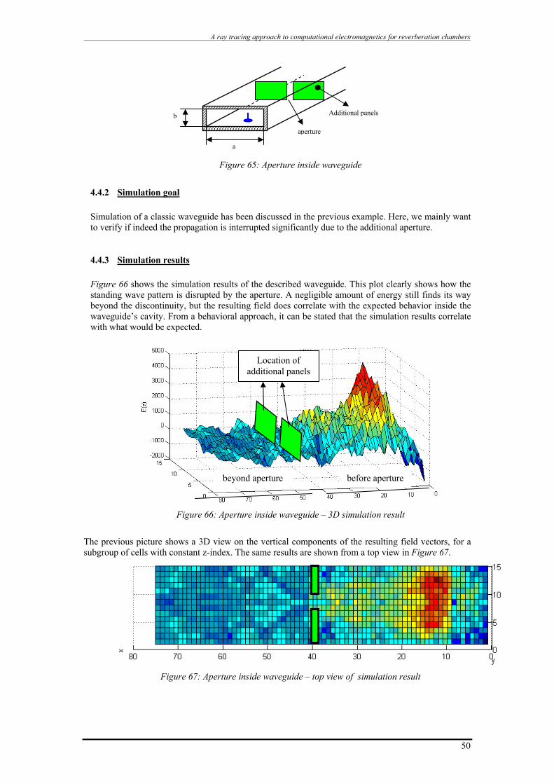
A ray tracing approach to computational electromagnetics for reverberation chambers
Additional panels
aperture
b
a Figure 65: Aperture inside waveguide
4.4.2 Simulation goal
Simulation of a classic waveguide has been discussed in the previous example. Here, we mainly want to verify if indeed the propagation is interrupted significantly due to the additional aperture.
4.4.3 Simulation results
Figure 66 shows the simulation results of the described waveguide. This plot clearly shows how the standing wave pattern is disrupted by the aperture. A negligible amount of energy still finds its way beyond the discontinuity, but the resulting field does correlate with the expected behavior inside the waveguide’s cavity. From a behavioral approach, it can be stated that the simulation results correlate with what would be expected.
Location of additional panels
Figure 66: Aperture inside waveguide – 3D simulation result
The previous picture shows a 3D view on the vertical components of the resulting field vectors, for a subgroup of cells with constant z-index. The same results are shown from a top view in Figure 67.
Figure 67: Aperture inside waveguide – top view of simulation result
beyond aperture before aperture
50

A ray tracing approach to computational electromagnetics for reverberation chambers
4.5 Simulating a higher TE mode inside a rectangular waveguide
4.5.1 Description
Once again, a waveguide is considered. In this case, we enlarge the waveguide’s width (i.e. a = 2λ), which should cause the creation of a higher mode in the standing wave pattern inside the wave guide’s cavity.
4.5.2 Simulation goal
The goal for this simulation is to verify whether the calculated resulting vector field will indeed show a standing wave pattern which can be correlated to the expected theoretical behavior.
4.5.3 Simulation results
Figure 68 shows the simulation results of the described waveguide configuration. Similarly as for the previous examples, only the vertical vector component of a layer of the resulting vector field is shown.
Figure 68: Next mode inside waveguide – top view of simulation results
To illustrate how the results as shown in Figure 68 look like before rotation, a 3D plot is shown in Figure 69. This 3D plot is exactly the same plot as section 1 in Figure 68, after rotation.
Figure 69: section 1 in 3D view
Monopole
Section 1length
2λ
Section 3
Section 2
Location monopole
51

A ray tracing approach to computational electromagnetics for reverberation chambers
Figure 68 is a composition of eight distinct simulations. Their individual results are positioned relative to each other in such a way that they visualize the first part of the waveguide’s cavity. The results clearly show a standing wave pattern. From a theoretical approach, the defined dimensions of this waveguide (a = 2λ and b << λ/2) should create a transversal electric mode TE50. The distribution of the TE50 mode is illustrated in Figure 70.
bWaveguide aperture
aElectric
field vector distribution
TE50 Figure 70: Waveguide TE50 mode
This field distribution should be present inside the waveguide’s cavity. Indeed, looking at the first part of the waveguide, near the transmitting monopole antenna (section 2 in Figure 68), a comparable situation can be distinguished. This is illustrated in Figure 71.
Figure 71: TE50 mode at front-end Figure 72: TE50 mode along the waveguide
Figure 72
At some other locations, one could state that the resulting vector field has the tendency to behave as theoretically predicted. As is shown in , section 3 (as indicated in Figure 68) also behaves like the theoretical model. However, this field distribution pattern does not repeat itself throughout the entire length of the waveguide (for the region that has been simulated). After further analysis of the results for this simulation, it was noticed that the current simulation environment is incomplete, in such a way that a full TE50 mode will never be created. In order to obtain a typical TE50 mode standing wave pattern, there need to be more then one monopole antenna.
a
b b
a
52
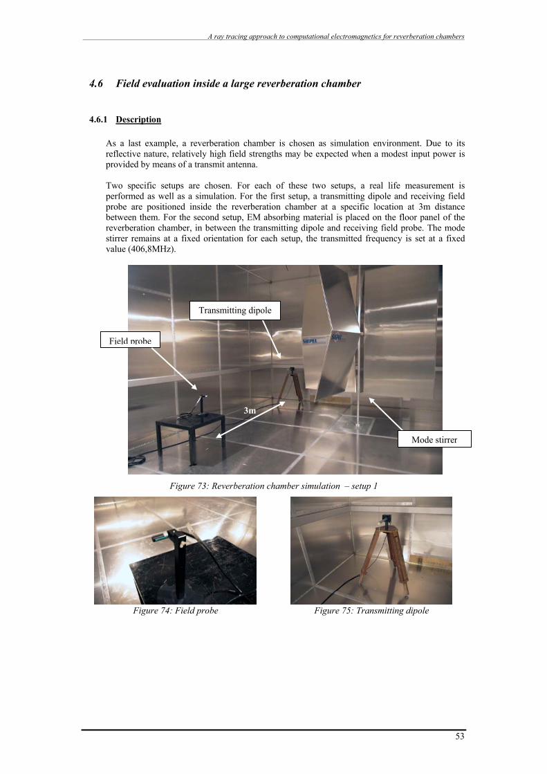
A ray tracing approach to computational electromagnetics for reverberation chambers
4.6 Field evaluation inside a large reverberation chamber
4.6.1 Description
As a last example, a reverberation chamber is chosen as simulation environment. Due to its reflective nature, relatively high field strengths may be expected when a modest input power is provided by means of a transmit antenna. Two specific setups are chosen. For each of these two setups, a real life measurement is performed as well as a simulation. For the first setup, a transmitting dipole and receiving field probe are positioned inside the reverberation chamber at a specific location at 3m distance between them. For the second setup, EM absorbing material is placed on the floor panel of the reverberation chamber, in between the transmitting dipole and receiving field probe. The mode stirrer remains at a fixed orientation for each setup, the transmitted frequency is set at a fixed value (406,8MHz).
Transmitting dipole
Field probe
3m
Mode stirrer
Figure 73: Reverberation chamber simulation – setup 1
Figure 74: Field probe Figure 75: Transmitting dipole
53
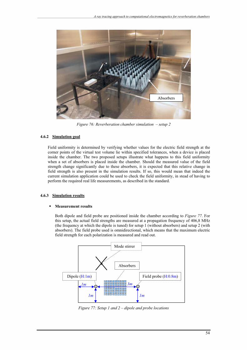
A ray tracing approach to computational electromagnetics for reverberation chambers
Absorbers
Figure 76: Reverberation chamber simulation – setup 2
4.6.2 Simulation goal
Field uniformity is determined by verifying whether values for the electric field strength at the corner points of the virtual test volume lie within specified tolerances, when a device is placed inside the chamber. The two proposed setups illustrate what happens to this field uniformity when a set of absorbers is placed inside the chamber. Should the measured value of the field strength change significantly due to these absorbers, it is expected that this relative change in field strength is also present in the simulation results. If so, this would mean that indeed the current simulation application could be used to check the field uniformity, in stead of having to perform the required real life measurements, as described in the standard.
4.6.3 Simulation results
Measurement results
Both dipole and field probe are positioned inside the chamber according to Figure 77. For this setup, the actual field strengths are measured at a propagation frequency of 406,8 MHz (the frequency at which the dipole is tuned) for setup 1 (without absorbers) and setup 2 (with absorbers). The field probe used is omnidirectional, which means that the maximum electric field strength for each polarization is measured and read out.
Figure 77: Setup 1 and 2 – dipole and probe locations
Field probe (H:0.8m)
3m
1m 1m
1m
Mode stirrer
Absorbers
Dipole (H:1m)
54

A ray tracing approach to computational electromagnetics for reverberation chambers
The following table represents the measured values. By adding absorbers at the specified locations, the field strength is lowered in amplitude by 4,77 dB (i.e. factor 1/3). A reduction in field strength is in fact expected, since part of the transmitted energy is damped by the absorbers.
Measured level [V/m]
Setup 1 59,7 Setup 2 20,4
Simulation results – simulation 1 A first simulation was performed by positioning a cube of 3375 cells (15 x 15 x 15 cells) at the location of the field probe. For these cells, the resulting field vector was calculated for setup 1 and 2 separately. The results are shown in Figure 78 and Figure 79.
Figure 78: Exyz for setup 1 Figure 79: Exyz for setup 2 The following pictures show the separation of both 3D vector fields into surface plots, representing vector fields E(x), E(y) and E(z) for an arbitrary chosen layer of the cell cube.
Figure 80: Ex for setup 1 Figure 81: Ey for setup 1 Figure 82: Ez for setup 1
Figure 83: Ex for setup 2 Figure 84: Ey for setup 2 Figure 85: Ez for setup 2 These pictures give a general idea about the field distribution inside the reverberation chamber, according to the simulation model. However, our simulation goal was to verify
55

A ray tracing approach to computational electromagnetics for reverberation chambers
56
whether the measured change in field strength, due to addition of absorbers, is also present in the simulation results. Since a numerical comparison needs to be made, additional operations on the resulting data set are necessary. In order to compare the calculated values, these values are mapped on a histogram. This histogram shows how many calculated field vectors have an amplitude for which the absolute value lies within one of the specified amplitude intervals. For both setups, such a histogram is created. These histograms are shown in Figure 86.
Setup 1 and Setup 2
0
20
40
60
80
100
120
140
1 6 11 16 21 26 31 36 41 46 51 56 61 66 71 76 81 86|E| Amplitude intervals
# ve
ctor
s
Setup 2Setup 1
Figure 86: Histogram field vector amplitude for setup 1 and 2
For both histograms, a region in the amplitude intervals can be distinguished which represents the majority of field vectors. Ideally, one would expect to find a difference between the two regions for both setups, according to the values that were measured. Such a clear distinction can not be found in the histograms however. Although the values for setup 1 (without absorbers) have the tendency to be slightly higher than the values for setup 2 (with absorbers), one could hardly state that this difference is in relative correlation with the measurements. Investigation of the contributing rays to the resulting field showed that indeed a large number of rays have a contribution for setup 1, where these rays no longer contribute for setup 2. This means that these rays are indeed absorbed by the additional foams. Another simulation was performed, where the influence of the size of each cell was investigated. The results for this simulation are summarized in the following paragraph.
Simulation results – simulation 2
For this second simulation, only one cell is used for which the resulting field vector is calculated. A relatively large cell size was chosen (0,1m), to avoid the effect of rays ‘missing’ the cell. For small cell sizes there might be a risk of rays missing the cells, which could result into misleading values. For both setup 1 and setup 2, the following results were calculated, where a reflection rate was set at 10:
Measured level [V/m]
Setup 1 57,9 Setup 2 55,8
These values still don’t match with the actual measured results.

A ray tracing approach to computational electromagnetics for reverberation chambers
Further analysis Until now, the simulation results fail to correlate exactly with the measured behavior. However, when considering the performed measurements it has to be mentioned that by shifting the position of the field probe by 0,05m, we get a significant change in field strength (20,4V/m to 11V/m). This means that the electric field behavior has rather abrupt changes in amplitude, strongly depending on the location in the reverberation chamber. For the simulation application, this means that a very high accuracy is needed. This high accuracy means that very small angle step sizes in between adjacent rays need to be taken, together with a large number of reflections (>20). In theory, these parameters would indeed lead to more accurate result. Simulation results are not deliverable however within the current time frame of the project.
57

A ray tracing approach to computational electromagnetics for reverberation chambers
5 Conclusion
5.1 General conclusion The simulation application delivers a resulting vector field. Looking at specific test cases, this vector field shows intuitive similarity to what would be expected for most cases. Some examples of test cases and more detailed analysis of their results are given in the previous section. The immunity assessment application was verified by measurement.
5.2 Results analysis
5.2.1 Can the field uniformity be determined? A resulting vector field at the eight corner points of the virtual test volume can be simulated. From a raw data file for example, it can be verified whether these values lay within the specified tolerances. Since these tolerances are expressed in dB, there is actually no need for absolute field values. This means that an exact determination of the output power from the transmit antenna is not required as an input value, since field uniformity can be evaluated, based on relative field values.
The results from section 4.6 have shown however that for larger dimensions of reverberation chambers, the accuracy of the current simulation application is insufficient. Accuracy is discussed in more detail in section 5.2.2. Under the assumption that valid results could be calculated, another downside exists. Suppose a broad frequency spectrum needs to be evaluated, then a simulation is required for each single frequency within this region. In practice this would mean that with a well considered frequency step size, the same simulation and evaluation routine needs to be performed for each successive frequency. Also, the mode stirrer movement is not taken into account. Each mode stirrer position has to be simulated by adding its dimensions to the simulation environment. During simulation, the user can define the current phase through the transmit antenna. This is a fixed value, which means that all other angles are not taken into account in the final result. All these aspects have as a consequence that quite a few simulations are needed with the current simulation application.
5.2.2 Accuracy During the development of the simulation application, several choices have been made which have their influence on the results’ accuracy: Spatial subdivision (Section 3.2.4) The continuous 3D volume for which a resulting vector field is to be simulated, is discretised into a group of cells. The cell sizes are uniform and user defined. The smaller the cells, the higher the resolution of the simulated field will be. However, for each cell a set of data needs to be kept in memory during the simulation process, which limits the total amount of cells. Therefore, the higher the resolution, the smaller the total simulated 3D volume will be, since the total number of cells ~ k³, with k the number of cells for each row in the cubic 3D vector field volume. Secondly, the chosen cell size also depends on the frequency used. A high frequency is associated with a short wavelength, therefore the higher the frequency, the smaller the cell size needs to be if for example standing wave patterns need to be visualized.
Initial angle step during ray tracing (Section 3.2.2)
The angular difference between two successive initial rays is defined by the end user. This angle has its influence on the accuracy of the final result, and is dependent on the chosen cell size. Suppose a very large angle step is used, where each cell has a very small cell size, then there is a
58

A ray tracing approach to computational electromagnetics for reverberation chambers
59
very high probability that some of these cells will not be reached by any ray. It should be the case that each single cell is intersected by an initial ray1, provided that there are no obstacles between the transmit antenna and this cell blocking any direct link between them. If this condition is not met, then for these non-intersected cells the final result is incorrect. In a first approach, a rule of thumb which can be applied here may be to use a maximal angle step α which equals:
)L.n2iarcsin(.2=α where i = cell size ,
n = max number of reflections, L = longest chamber dimension (3D diagonal between two opposite corners).
The longest theoretical path a ray may travel equals n.L. Assuming we would like to intersect each individual cell by an initial ray, we need to choose an angle step for which the distance between the rays at traveling distance n.L does not exceed the cell size. Figure 87 should clarify this. There is a disadvantage however. When looking at very high frequencies, it would be tempting to choose very small cell sizes. As a consequence, very small angle steps have to be chosen. This in turn leads to an increase in the number of iterations r, since 21~r α , which has its effect on the required processing time.
Figure 87: Determination or the minimal angle step
A trade-off needs to be made between a cell size which is sufficiently small (resulting into a sufficiently high resolution) and an angle step which is sufficiently high in order to have a satisfactory result within a reasonable time frame.
Maximum number of reflections (Section 3.3.3)
As was discussed earlier, a maximum number of reflections for each ray is taken into account. This maximum depends on a) maximum allowable memory consumption and b) allowable computation time. In theory, when reflection occurs on a highly conducting material, the reflection coefficient Γ will approximate to 1, which means that most of the incident energy is retransmitted. If Γ would equal 1, then we would in theory require an infinite number of reflections in order to have an exact determination of the resulting field. It is evident that during simulation a reasonable value has to be chosen. For a moderate personal computer (512MB RAM), ca.10 reflections is an acceptable maximum.
1 Initial ray: a ray with the transmit antenna as its origin, which has not yet intersected any reflecting or absorbing surface
Cell[ 1 1 1 ]
Cell[ 1 2 1 ]
Cell[ 1 3 1 ]
Cell[ 2 1 1 ]
Cell[ 2 2 1 ]
Cell[ 2 3 1 ]
Ray1
Ray2
Ray3
α/2 α/2
n.L
i

A ray tracing approach to computational electromagnetics for reverberation chambers
5.3 Future work
The project that was carries out in this thesis was quite interesting and ambitious and can easily be extended into several PhD projects. However, as the project already quite exceeded the regular Master thesis project time, and its results have reached a state in which they can be confronted with reality, we decided to round off the Master project. This leaves a number of issues to be considered:
There still remains a lot of work to be done to improve the application’s accuracy, required
processing power and memory consumption; the current solution can most likely be reviewed in order to increase its speed and to decrease its memory usage. For example, inside or outside verification is now based on the solution of goniometric functions, which could be translated into an algebraic approach relying on matrix transformations for example, leading to shorter computational time and more accurate results. Another example is that for now, a first approach to the ray tracing algorithm is applied. The algorithm itself could be modified by using ray tracing optimization techniques. An important aspect of the ray tracing technique is the search for intersections. This procedure can fundamentally be compared with a O(n) search algorithm, with n the number of objects. By grouping the objects into sets, where such sets can be discarded quickly, the intersection algorithm could be turned into a O(log n) algorithm. A set can be implemented as a bounding box or sphere. Implementation of these aspects will most likely lead to better performances for large dimension simulation environments where a high amount of reflections is required.
A more mathematical approach on the numerical inaccuracy could be made as well. This would allow verification of fault propagation throughout the sequence of iterative steps of the simulation application. If such a verification is possible, proper adjustments to the algorithms could be made, thus improving accuracy and performance, as stipulated above.
Addition of a specifically modeled database with short access time could avoid the consumption
of memory space. The application domain could also be expanded in such a way that not only rectangular surfaces
can be added, but also spherical or elliptic volumes. This could be done by applying the same underlying algorithm (with minor modifications), extended with the translation of a spherical surface into a set of distinct partial plane equations. With more significant adjustments to the algorithm, the sphere surface equation could be applied as well. It is suggested to check the existing techniques in the domain of visualization.
The visualization of the resulting field is now done by relying on a separate program, Matlab,
which allows this visualization through a more generic approach, without many possibilities for manipulation. This visualization could be part of the application itself, in such a way that it is optimized for the current domain of interest. This part is not implemented for the current project, but visualization of vector field is an existing research domain.
There could also be the possibility to add multiple transmit antennas in stead of only one. This
expansion would require minor adjustments to the underlying algorithm, since it would only mean that an identical iterative process has to be repeated for each added antenna, where the resultant field vector for each cell now has to be recalculated for all intersecting rays of each single antenna.
The current version of the application only allows cell group definition by placing all cells in a
cubic volume. This is not always the most optimal way to group the cells. When we are only interested in field vectors located on a plane for example, we would like to be able to define a plane-like grouping of cells.
60

A ray tracing approach to computational electromagnetics for reverberation chambers
5.4 Design process analysis
During the design process of this project, some engineering principles have proven their usefulness. First of all, preparation is necessary. In the earlier stages of the design of the simulation application, a review was made on different possible technical solutions for computational electromagnetics within this context. This was done not only by a theoretical approach based on literature, but also by visiting several research groups from the Katholieke Universiteit Leuven and Ghent University. After having developed an overview of these existing techniques, it was decided to follow the route of ray tracing in an adopted form. Secondly, documentation of choices and assumptions is essential. During the design of the project, a series of design choices were made. Part of these choices and decisions lead to an acceptable solution. The other part of these decisions had to be reviewed. In such case, documentation allows backtracking in order to find a more appropriate solution for the computational problem at hand. Thirdly, respecting a predefined time schedule is never easy. In the given circumstances, a combination had to be found between a set of timing schedules, both for this project as well as for a wide variety of other work-related projects. In a personal opinion, the key to optimized completion of each individual project is first to identify a set of milestones for each project. As a next step, each of these milestones have to be ranked in sequential order, as well as in order of importance. As a final step, for each current project in turn, the most important milestone has to be dealt with. Once this milestone is reached, the next project is treated. This method avoids the risk of neglecting all lower order projects.
61

A ray tracing approach to computational electromagnetics for reverberation chambers
6 References [CRO1] Cross, A.W. (1965). Experimental Microwaves. Stevenage: Sanders. [DGR1] De Greve,B. (2007). Reflections and Refractions in Ray Tracing [DHE1] Heam, D., & Baker, P. (2003). Computer Graphics with OpenGL. New Jersey:
Pearson Prentice Hall. [DO160] EUROCAE (1997). RTCA DO-160D – Environmental conditions and test procedures
for airborne equipment. Washington, DC: RTCA. [EMC1] European parliament and the council of the European Union (2004). Directive
2004/108/EC. Retrieved from http://eur-lex.europa.eu/ [FDI1] Diouf, F. , Paladian, F., Fogli, M. & Chauvière,C. (2007). Emission in Reverberation
Chamber: Numerical Evaluation of the Total Radiated Power by a Dipole with Stochastic Collocation Method. EMC Zurich 2007. 18th International Zurich Symposium.
[FOL1] Olyslager, F., Fostier, J., Peeters, J., & De Zutter, D. (2007). Fast and Accurate Evaluation of Enclosures With the Method of Moments by Using Splay Trees. , EMC Zurich 2007. 18th International Zurich Symposium.
[GOE1] Goedbloed, J.J. (1993). Elektromagnetische compatibiliteit. Antwerp: Kluwer. [GRE1] Goral, C.M., Torrance, K.E., Greenberg, D.P., & Battaille, B. (1984). Modeling the
Interaction of Light Between Diffuse Surfaces. ACM SIGGRAPH Computer Graphics, 18, 213 – 222.
[HOL1] Holloway, C.L. (2005). Reverberation Chambers for EM Applications [PowerPoint slides]
[HUB1] Hubing, T.H. (1997). An EMC Engineer’s guide to Electromagnetic Modeling Software [PowerPoint slides]. Retrieved from http://www.ieee.ca/diglib/library/ 9712hubing/hubing.pdf
[IEC421] IEC (2000). IEC 61000-4-21. Switzerland:IEC Central Office [KKY1] Kythe,K. (1995). Introduction to Boundary Element Methods (Symbolic and Numeric
Computation Series). CRC Press. [LAE1] Laermans, E., Knockaert, L., & De Zutter, D. (2004). Two-dimensional method of
moments modeling of lossless overmoded transverse magnetic cavities. Journal of Computational Physics, 198, 326 – 348.
[LAU1] Laurenson, D.I. (1994). Indoor Radio Channel Propagation Modeling by Ray Tracing Techniques. Retrieved from http://www.see.ed.ac.uk/~dil/thesis_mosaic/ total.html
[MPI1] Piette, M., Moesen, K., & Montezuma, S. (2006). Complete space – time validation of a single mode-stirrer reverberation chamber for immunity testing. [PowerPoint slides]
[VLI1] Van Lil, E., & Trappeniers, D. (2006). EPICS – user guide.
[WAI1] Wait, J.R.(1986). Introduction to antennas & propagation. England: Short Run Press Ltd.
[WAL1] Wallyn, W., De Zutter, D., & Laermans, E. (2003). Fast Shielding Effectiveness Prediction for Realistic Rectangular Enclosures. IEEE transactions on electromagnetic compatibility, 45, 639 – 643.
[WAL2] Wallyn, W., De Zutter, D., & Rogiers, H. (2002). Prediction of the Shielding and Resonant Behavior of Multisection Enclosures Based on Magnetic Current Modeling. IEEE transactions on electromagnetic compatibility, 44, 130 - 138.
62

A ray tracing approach to computational electromagnetics for reverberation chambers
Appendix A
A.1 An example of ray and plane intersection To illustrate the above, we consider one of the walls of the reverberation chamber. As input parameters to define the size and location of this wall, it is required to provide Cartesian coordinates of three points on the plane (where these three points are not collinear). These might be the corner points of that wall, for example:
γ
Y
Z
(0,0,0)
(300,0,200)
ζ
(300,0,0)
PPb
Pa
X
Figure 88: example of ray/plane intersection
Following points are given to define plane ζ: e.g. P1(0,0,0), P2(300,0,0) and P3(300,0,200) Following points are given to define ray γ: e.g. Pa(300,100,100) and Pb(600,400,100) The Cartesian plane equation (2) can be derived as follows: A.x + B.y + C.z +D=0
≡ 0zyxzyxzyx
z.1yx1yx1yx
y.z1xz1xz1x
x.zy1zy1zy1
3P3P3P
2P2P2P
1P1P1P
3P3P
2P2P
1P1P
3P3P
2P2P
1P1P
3P3P
2P2P
1P1P
=−++
≡ y = 0 in this example We can then calculate s as follows:
s = )zz(C)xx(B)xx(A
Dz.Cy.Bx.APbPaPbPaPbPa
PaPaPa
−+−+−+++
≡ s = -1/3 in this example Finally, point of intersection P equals Pa + s(Pb – Pa), which is P(200,1,0) in our example
As a remark, s can either have one of the following values: 0<s<1: intersection occurs between Pa and Pb s=0: intersection occurs on Pa s=1: intersection occurs on Pb s>1: intersection occurs after Pb s<0: intersection occurs before Pa, at a distance s(Pb – Pa) from Pa.
63

A ray tracing approach to computational electromagnetics for reverberation chambers
Appendix B
B.1 Derivation of equations for E and H in a Cartesian system Following equation can be derived:
AHrrr
×∇=
zyx AAAzyx
kji
∂∂
∂∂
∂∂≡
rrr
with ir
, jr
and kr
the unit vectors for Cartesian axis X,Y and Z
jxAi
yA zz rr
∂∂
−∂∂
≡ with Ax and Ay = 0
The magnetic vector H
r can be decomposed in its Cartesian components Hx, Hy and Hz , using the
result above:
=xHy
Az
∂∂
=yHxAz
∂∂
−
= 0 zH By substituting these results into the Maxwell equation for the electric field component of the electromagnetic wave, we obtain:
( ) HEj rrr
×∇=ωε+σ
zyx HHHzyx
kji
∂∂
∂∂
∂∂≡
rrr
ky
Ax
Ajzy
Aizx
A2
z2
2z2z2z2 rrr
⎟⎟⎠
⎞⎜⎜⎝
⎛
∂
∂−
∂
∂−+
∂∂∂
+⎟⎟⎠
⎞⎜⎜⎝
⎛
∂∂∂
−−≡
As for the magnetic vector, the electric vector E
r can also be decomposed into components Ex, Ey and
Ez:
( ) =ωε+σ xEjzx
Az2
∂∂∂
( ) =ωε+σ yEjzy
Az2
∂∂∂
−
( ) =ωε+σ zEj2
z2
2z2
yA
xA
∂
∂−
∂
∂−
64

A ray tracing approach to computational electromagnetics for reverberation chambers
65
B.2 Derivation of EZ equation in terms of magnetic vector potential Ez can alternatively be formulated by using the earlier proposed equation for in terms of the magnetic vector potential:
Er
( )[ ]AAj
1E 2 rrrrr•∇∇+γ−⋅
ωε+σ= with ( )εω+σμω=γ jj2
([ )zz2
z AAj
1E •∇∇+γ−⋅ωε+σ
=≡rr ] with ( )εω+σμω=γ jj2
⎥⎦
⎤⎢⎣
⎡∂
∂+γ−⋅ωε+σ
=≡ 2z
2
z2
z zAA
j1E
B.3 Simplification of HΦ equation for far field conditions
( ) θγ+⋅π
= γ−φ sin.e.r1
r4dl.IH r.
20
r
( ) θγ+⋅π
=≅ γ−φ sin.e.r1
r4dl.IH r.
20
r with ( )εω+σμω=γ jj2
( )ωεωμ=γ 002 jj for free space
200
2 ωεμ−=γ
200
2 ωεμ−=γ
jk=γ with ck ω=
and 00c με=
θ⋅π
=≅ −φ sin.e
r4dl.IjkH r.jk0
r
B.4 Vector potential equation for half wavelength dipole
Originally, it was stated that the magnetic vector potential Ar
z for a Hertz dipole can be expressed as:
r.0z e.
r4dlIA γ−
π=
r
However, for a dipole with considerable length L and the constant current distribution as described in Figure 33, some adjustments need to be made to the equations of A
rz. Primarily, I0.dl needs to be
replaced by I(z), which is formulated within free space conditions (σ = 0, ε = ε0, μ = μ0, γ = jk with k = ω 00με = ωc) as follows

A ray tracing approach to computational electromagnetics for reverberation chambers
⎥⎦
⎤⎢⎣
⎡⎟⎠⎞
⎜⎝⎛ −= z
2L.ksin.I)z(I m
From observation point P, which lies at distance R from the dipole (where R is assumed to lie within the far field region), the dipole can be considered to consist of a finite set of Hertz dipoles with length dz, each contributing in the resulting field components by creating a magnetic vector potential dAz. In order to capture each contribution dAz, the integral is taken over the total length of the dipole. Together with the equation for I(z), A
rz can be rewritten:
dz.R
e.z2Lksin.
4IA
R.k.j2/L
2/L
mz
−
−∫ ⎥
⎦
⎤⎢⎣
⎡⎟⎠⎞
⎜⎝⎛ −
π=
r
Since we assumed that R is sufficiently large so that P will lie in the far field region, we may claim that R ≈ r. However, the difference in distance does have an impact on the phase difference between path r and path R. This needs to be taken into account for each different Hertz dipole dz as follows:
θ−−
≅ cos.z.k.jr.k.jR.k.j
e.r
eR
e
The last part of the equation denotes the phase difference. The following picture visualizes this situation.
Z
Figure 89: difference in traveling distance for each individual Hertz dipole
Again, taking the above considerations into account, and resolving the integral, we can derive an adopted equation for the magnetic vector potential:
( )⎥⎥
⎦
⎤
⎢⎢
⎣
⎡
θ
−θ
π=
−
2
r.k.jm
z sin.k
)2L.kcos(cos.2
L.kcos.
r4e.IA
r
dz
Rθ
r
towards P in far
field region
z
r – R = z.cos θ
66

A ray tracing approach to computational electromagnetics for reverberation chambers
Appendix C
1. Defining chamber properties As a first step, the chamber properties need to be set out. This means that a user has to define the chamber dimensions, as well as the dimensions and positions of all additional walls or panels (e.g. the panels on a mode stirrer). This is done by allowing the input of chamber length, width and height. As input values, the user can also define each panel by giving the Cartesian coordinates of three successive corner points of an additional panel. Both methods allow determination of the corresponding plane equations. Identification of the corner points allow verification of intersection through a inside-outside tests as discussed in section 3.2.1. Finally, each panel or wall is associated with a reflection coefficient Г. During calculations, -Г is used for field components which are parallel to the intersected plane, in order to attain a 180° shift in phase, as discussed in section 3.3.3.
Figure 90: User interface - quantification of chamber properties
2. Transmit antenna and cell group settings The next step in setting up a simulation project is the definition of antenna and cell group parameters. For the antenna, the position and orientation (azimuth and elevation) need to be user defined. This is done by Cartesian coordinates with respect to the chamber origin. Each initial ray originates from this position. The angle step between each individual ray is also user defined, and determines the ray equation as was explained in section 3.2.2. The last required antenna parameter is the antenna
Chamber dimension
Additional plane
dimensions and positions
67

A ray tracing approach to computational electromagnetics for reverberation chambers
radiation pattern as shown in Figure 15, which should give a relative excitation value (dBi) for each individual ray. The dBi value corresponds to the forward gain of the antenna, compared to the hypothetical isotropic antenna, which uniformly distributes energy in all directions. The radiation pattern can be loaded from an external file. When angle step for individual ray generation and angle step for antenna radiation pattern definition differ, a 3D interpolation is used to find the intermediary result. As explained in section 3.2.4, a part of the environment is divided into separate cells, where for each of them the simulation application calculates a resulting field vector (magnitude and orientation). This group of cells is identified by the location of its origin, the number of cells for each row and the individual cell size. All these parameters are defined by the user.
Antenna parameters
Antenna radiation pattern
Cell group parameters
Figure 91: User interface –transmit antenna and cell group settings
3. Simulation project settings Before a simulation can be run, the maximum number of reflections, the current Im through the antenna and its initial phase need to be given (Figure 92). Once these parameters are defined, the simulation can be initiated.
68
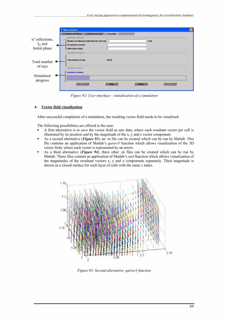
A ray tracing approach to computational electromagnetics for reverberation chambers
n° reflections, Im and
Initial phase
Total number of rays
Simulation progress
Figure 92: User interface – initialization of a simulation
4. Vector field visualization After successful completion of a simulation, the resulting vector field needs to be visualized. The following possibilities are offered to the user: A first alternative is to save the vector field as raw data, where each resultant vector per cell is
illustrated by its position and by the magnitude of the x, y and z vector component. As a second alternative (Figure 93), an .m file can be created which can be run by Matlab. This
file contains an application of Matlab’s quiver3 function which allows visualization of the 3D vector field, where each vector is represented by an arrow.
As a third alternative (Figure 94), three other .m files can be created which can be run by Matlab. These files contain an application of Matlab’s surf function which allows visualization of the magnitudes of the resultant vectors x, y and z components separately. Their magnitude is shown as a closed surface for each layer of cells with the same z index.
Figure 93: Second alternative: quiver3 function
69

A ray tracing approach to computational electromagnetics for reverberation chambers
Magnitude Z-component
length
width
Figure 94: third alternative: surf function for a group of cells with identical z-index
70

A ray tracing approach to computational electromagnetics for reverberation chambers
Appendix D
1. Context Analysis of the immunity assessment application The measurement application allows the automation of an immunity assessment. The stakeholders are the test engineers, who initialize a test sequence and will in fact be the users of the application, and on the other hand the distributor or developer who is responsible for the device being assessed. Besides the reverberation chamber, other equipment will be used during an immunity test session, like function generators, amplifiers, antennas, a mode stirrer and field power sensors. Before an immunity test can be started, these devices need to be imported into the application. This import should include relevant equipment characteristics for each item, such as minimal and maximal usable frequency, and a driver, allowing communication with the equipment. There should also be possibilities to alter and manage the available equipment library. The immunity assessment itself will start with the initialization of a test project. This means that the test engineer will provide the necessary parameters to the application, in order to enable the start-up of a complete test sequence. First of all, a frequency domain within which the immunity of a test object will be evaluated, is specified. Within this domain, a frequency dependant EM field strength, a modulation type and dwell time are required. There should also be a way to define the frequency step size and the number of stirrer rotations for each frequency. All these parameters will define the test setup. A next step when initializing the test project is the selection of the test equipment which will be used during the assessment. By specifying the test setup, the choice amongst all available test equipment, which are part of the specified equipment library, is limited (each generator for example can only be used within the boundaries of its operational frequency range). It is therefore possible to restrict the test engineers’ choice when making a selection, in order to avoid inconsistencies. Another important aspect when selecting the equipment is that the test engineer can define a list of equipment of each type, each within its partial frequency sub domain. For example, a generator can be chosen to be used up to a certain frequency. When the assessment process reaches this frequency, another generator is specified as the one to be used for the higher frequencies. After this second generator a third one may be specified, etc. This leads to adjacent frequency sub domains, each with its own list of test equipment to use. The goal here is to cope with the limited useable frequency range of the test equipment; it is now possible to specify one complete immunity test project with different test equipment to be used for adjacent frequency sub domains. An example is shown in the next figure: Total frequency domain subdomain 1 subdomain 2 subdomain 3 subdomain 4
Selected Generators: Generator 1 Generator 2 Generator 3 Generator 4
Figure 95: Selection of test equipment,e.g. generators
After definition of test setup and consistent completion of equipment selection, the immunity assessment can be initialized. During the immunity test, a high EM field strength will be generated. The level of field strength might be higher then the maximum tolerable field strength of the field sensors. This means that excessive radiation might lead to permanent damage to these sensors, which is
71

A ray tracing approach to computational electromagnetics for reverberation chambers
of course not acceptable. The necessity to measure the (mostly high level) radiated field strength and the limited usage in terms of field strength of the field sensors lead to two apparently mutual exclusive situations. However, due to the linear behavior of the field strength in relation to the input power, it is possible to first measure the field strength for a certain frequency with a lower input power to the transmit antenna. Then, after removing the field sensor from the reverberation chamber, it can be calculated how much the input power must be increased, in order to reach the requested field strength without having to actually measure it with a field sensor. By registering the stirrer rotation angle for which a maximal field strength is reached with low input power, the high level test must only be performed for this rotation angle as well. This process requires a manipulation by the test engineer; he or she needs to remove the sensor from the chamber in between the low level and the high level field strength process. Since every manipulation is time (and inherently money) consuming, it is decided to combine the removing of the field sensor with the replacement of test equipment when the end of their frequency sub domain is reached (as explained above). In short this means that the low level process is performed at successive frequencies, until a frequency x is reached for which a test equipment needs to be changed. Instead of changing this equipment, the field sensor is removed, the current frequency is reset and the frequency sweep is repeated with higher input power in order to attain the requested high field strength. Only when frequency x is reached for the second time, the test engineer is allowed to replace the equipment and to put the field sensor back in place. An identical iteration is repeated for the next frequency sub domain. During the entire immunity assessment process, the test engineer is capable of tracking the test progress. In short, the main processes in which the system and its environment are involved are device parameterization, initialization of test setup and tracking the test sequence.
2. Requirement Analysis
2.1. User requirements Following paragraphs show the different use cases from the point of view of the users. The process models will be shown later on. Adding new test equipment to the device library The user adds new equipment to the equipment library. First the user specifies the type of equipment that needs to be added: function generator, amplifier, field sensor, antenna or mode stirrer. Next, he or she specifies the relevant parameters for this type of device and loads the device driver for this equipment. Each entry made by the user is verified for consistency and correctness. Changing equipment specifications in the device library The user wants to change formerly specified parameters of certain equipment in the device library. First of all, the user opens a view to the library, which enables selection of the desired equipment by its name. Next, the user changes the parameters of the selected equipment. Removing equipment from the device library The user removes equipment from the device library simply by selecting the desired item and deleting it. Initializing an immunity test The user can initialize an immunity test in two ways. First of all, he can decide to build up the test setup from scratch. This means that the desired setup needs to be filled in completely. When the user has specified a test setup, he can save this into memory as a project file. Before saving is possible, the setup is verified for consistency and correctness. As an alternative, the user may
72

A ray tracing approach to computational electromagnetics for reverberation chambers
decide to load an existing project file. This project file contains a consistent setup, since this was verified at the moment that this latter setup was saved earlier. At this level, the required parameters are:
- Frequency domain A global start and stop frequency are specified. This frequency domain is further divided into smaller, adjacent frequency sub domains. For each of these sub domains, the user specifies a frequency step size to be taken by the system during test execution.
- Mode tuning Again, the global frequency domain is divided into smaller adjacent sub domains. For each of the sub domains, a rotation step angle for the mode stirrer is specified. This value defines the number of discrete mode stirrer rotation steps there need to be for each frequency during test execution.
- Field strength Once more, the global frequency domain is divided into smaller regions, where for each of them the desired field strength is defined.
- Modulation The modulation that is to be excited by the transmit antenna.
As a next step, the user must specify which devices he wishes to use. For each type of device (generator, amplifier, antenna or field power sensor) a part of the device library is made available for the user to select, where it is always verified whether or not the usage range for a selected device lies within this devices’ usable range. Running an immunity test An immunity test run needs to be preceded by a test setup initialization. This setup contains all the data the system needs to be able to perform a complete immunity test, according to the user specifications. After starting the test, a user may decide to abort the test run at any given moment. It must also be possible to freeze the test run at a certain frequency, with a choice whether or not the input power is switched on or off.
3. Application Model
3.1. Object model The object model for this application is represented as a simplified class diagram. Most of the user and system actions are related to handling the represented data.
Constraints for the object model: - This class diagram depicts the data layer, which will be referred to later in this document. - Class ‘devices’ is a generalization of a set of different types of devices, i.e. generators,
amplifiers, mode stirrers, field probes and antennas, as mentioned earlier. Common parameters are a name, a short description of the device and its minimal and maximal usable frequency.
- Each immunity measurement project consists of some parameters, which define the margins for the required immunity test run.
- Each project will be linked to a collection of devices (an initial proposal will be made by the system, but it should be easily overridden by the end user). The goal here is to avoid any gaps during the execution of a project, where for a required functionality (e.g. field measurement) no device is specified. Also, this indirect link between project and device library, in stead of having a direct link (through a project parameter for example), allows the system to redefine the project/devices list in case a certain device is deleted by the user, or in case its parameters are changed.
- For each project, there exist a number of possible executions (0 to infinity). This execution is in fact the test session being executed.
73

A ray tracing approach to computational electromagnetics for reverberation chambers
Project execution
Start time
Figure 96: Object Model
3.2. Process models for Use Cases
Adding new equipment to the device library
1. User selects device type to add (either generator, amplifier, mode stirrer, antenna or field power
sensor) (select) 2. User adds device specifications (specify) 3. User tries to save the specified device parameters (save)
Figure 97: use case – adding device
Devices
Name Description Min.freq. Max freq.
Generator
Max output P Modulations Driver
Amplifier Mode Stirrer Field Probe Antenna
Max P In Max P Out
Driver Max EV Driver
Gain pattern (tbd)
Stop time nextFreq nextEV
0 .. * nextStirrerRot Immunity Project
StartFreq StopFreq Project/devices Steptype Modulation 0 .. * StartFreq 1 .. 1
StopFreq Stirrersteps (intervals) Frequencysteps (intervals)
0 .. * Fieldstrength (intervals)
1 .. 1
Name
select specify save
Inconsistent input
start end
74

A ray tracing approach to computational electromagnetics for reverberation chambers
Deleting equipment from the device library
1. User selects device to be deleted by its name (select) 2. user saves the changes (save)
Figure 98: use case – deleting device
Changing equipment specifications in the device library
1. User selects device for which the parameters need to be updated. Selection is made by name
(select) 2. User specifies new values for the desired parameters (update) 3. User saves changes (save)
Figure 99: use case – changing device parameters
Initializing an immunity test
1. User loads an existing test setup (load) 2. User starts building up a test setup from scratch (new) 3. User modifies the test setup parameters (modify)
- Start or stop frequency - Modulation - Linear or logarithmic frequency step type - Frequency step list - Stirrer rotation step list - Field strength list - Dwell time
4. user tries to save the test setup (setup save) 5. user selects equipment to use from device library (device selection) 6. user can review the setup after the devices are selected (review)
select update save
Inconsistent input
start end
start select save end
75
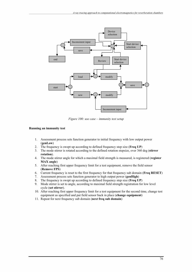
A ray tracing approach to computational electromagnetics for reverberation chambers
Figure 100: use case – immunity test setup
Running an immunity test
1. Assessment process sets function generator to initial frequency with low output power (genLow)
2. The frequency is swept up according to defined frequency step size (Freq UP) 3. The mode stirrer is rotated according to the defined rotation stepsize, over 360 deg (stirrer
rotation). 4. The mode stirrer angle for which a maximal field strength is measured, is registered (register
MAX angle) 5. After reaching first upper frequency limit for a test equipment, remove the field sensor
(Remove FPS) 6. Current frequency is reset to the first frequency for that frequency sub domain (Freq RESET) 7. Assessment process sets function generator to high output power (genHigh) 8. The frequency is swept up according to defined frequency step size (Freq UP) 9. Mode stirrer is set to angle, according to maximal field strength registration for low level
cycle (set stirrer). 10. After reaching first upper frequency limit for a test equipment for the second time, change test
equipment as specified and put field sensor back in place (change equipment) 11. Repeat for next frequency sub domain (next freq sub domain)
start
new
Inconsistent input
load modify
modify
save
Inconsistent input
Start device selection
Device selection
save
end Start device selectionReview
76
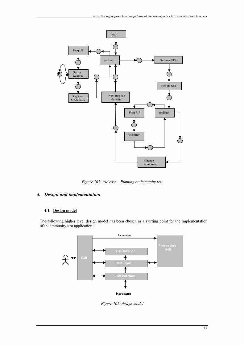
A ray tracing approach to computational electromagnetics for reverberation chambers
start
Figure 101: use case – Running an immunity test
4. Design and implementation
4.1. Design model
The following higher level design model has been chosen as a starting point for the implementation of the immunity test application :
Figure 102: design model
genLow
Freq UP
Remove FPS
genHigh Freq UP
Change equipment
Freq RESET
Next freq sub domain
Stirrer rotation
Register MAX angle
Set stirrer
Parameters
Processing unit Visualization
GUI Data layer
HW Interface
Hardware
77

A ray tracing approach to computational electromagnetics for reverberation chambers
The following modules can be distinguished: HW interface The hardware interface ensures communication between the application and the test equipment. Direct communication between the user and the hardware is possible through the graphical user interface (GUI). During system operation, the HW interface will get the command set, which is necessary for communication and is incorporated in the device driver, via the data layer. GUI The graphical user interface delivers an easy to use tool to the user. Every use case, i.e. every action the user might perform which is related to the systems’ operation, will have to be performed through this module. Data Layer The data layer takes care of the efficient management of data storage. This means the equipment and project libraries, as well as measurement and simulation results. Visualization This layer will provide an interpretable visualization of measurement and simulation results. These results will be provided to the GUI for further manipulation by the user. Processing unit The processing unit will perform all necessary calculations. Its main focus will be to solve field equations during simulations, which is further elaborated in the second part of this document.
4.2. Implementation
a) Hardware interface
By using the Java Native Interface (JNI), it is possible to declare native methods from a Java class. This means that from within a Java object, a method can be called for which the method definition is in fact native code, like C. Java JNI is contained in the Java Development Kit (JDK). The motivation to use JNI for this project is that the application has to be able to communicate with measuring equipment through the GPIB IEEE 488.2 (general Purpose Interface Bus) protocol. On the other hand, the application also needs to be able to support graphical capabilities (GUI module). Java is a good choice to deliver solutions for graphical interfaces, but there does not exist an API which enables communication over the GPIB 488.2 protocol, where this is possible when using C. National Instruments for example, who provides GPIB controllers, supports the usage of a GPIB header decl-32.h, which contains functions like ibdev, ibrd and ibwrt. These functions can be used during communication over the GPIB bus using C-code. For this reason, it was decided to divide the raw communication with the test equipment (C-code) and communication wich the user through a GUI (Java-code), where JNI serves as an interpreter between the both languages.
78
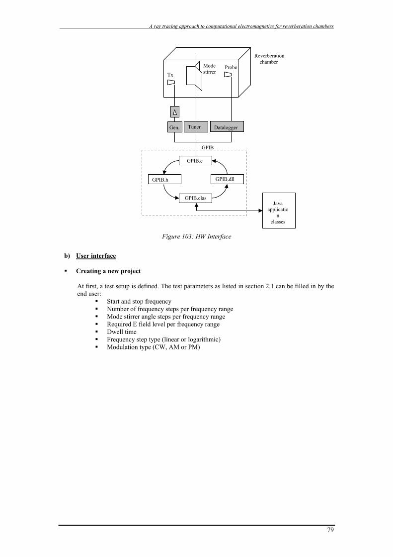
A ray tracing approach to computational electromagnetics for reverberation chambers
Reverberation chamber
Mode Probe stirrer Tx
Tuner Gen. Datalogger
GPIB
GPIB.c
GPIB.dll GPIB.h
GPIB.clasJava
application
classes
Figure 103: HW Interface
b) User interface
Creating a new project
At first, a test setup is defined. The test parameters as listed in section 2.1 can be filled in by the end user:
Start and stop frequency Number of frequency steps per frequency range Mode stirrer angle steps per frequency range Required E field level per frequency range Dwell time Frequency step type (linear or logarithmic) Modulation type (CW, AM or PM)
79

A ray tracing approach to computational electromagnetics for reverberation chambers
Figure 104: RI test setup interface
Device selection
After a test setup is defined, the appropriate devices can be selected. Based on the given frequency ranges, a list of possible devices is automatically generated. This avoids the selection of devices which can not be operated in the specified frequency range.
Figure 105: RI device selection interface
80
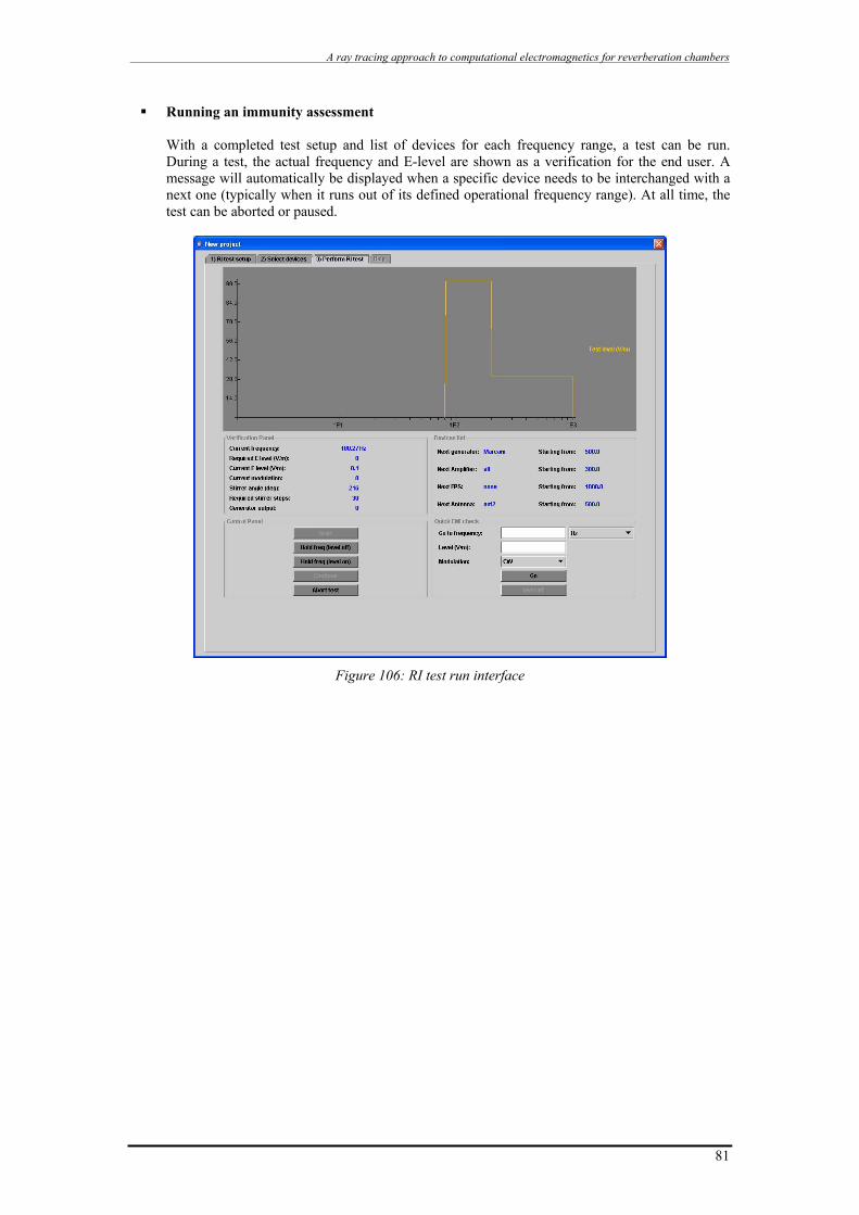
A ray tracing approach to computational electromagnetics for reverberation chambers
Running an immunity assessment With a completed test setup and list of devices for each frequency range, a test can be run. During a test, the actual frequency and E-level are shown as a verification for the end user. A message will automatically be displayed when a specific device needs to be interchanged with a next one (typically when it runs out of its defined operational frequency range). At all time, the test can be aborted or paused.
Figure 106: RI test run interface
81

A ray tracing approach to computational electromagnetics for reverberation chambers
82