Eigenvarieties, families of Galois representations, p-adic...
233
Eigenvarieties, families of Galois representations, p-adic L-functions Incomplete notes from a Course at Brandeis university given in Fall 2010 1
Transcript of Eigenvarieties, families of Galois representations, p-adic...
Eigenvarieties, families of Galoisrepresentations, p-adic L-functions
Incomplete notes from a Course at Brandeis university given in Fall 2010
1


Contents
Introduction 9
Part 1. The ’eigen’ construction 11
Chapter I. Construction of eigenalgebras 13
I.1. A reminder on the ring of endomorphisms of a module 13
I.2. Construction of eigenalgebras 14
I.3. First properties 15
I.4. Behavior under base change 17
I.5. Eigenalgebras over a field 18
I.5.1. Structure of Spec T 18
I.5.2. System of eigenvalues, eigenspaces and generalized eigenspaces 18
I.5.3. Systems of eigenvalues and points of Spec T 19
I.6. The fundamental example of Hecke operators acting on a space of
modular forms 21
I.6.1. Complex modular forms and diamond operators 21
I.6.2. Hecke operators 22
I.6.3. A brief reminder of Atkin-Lehner’s theory 23
I.6.4. Hecke eigenalgebra constructed on spaces of complex modular forms 25
I.6.5. Eigenalgebras and Galois representations 28
I.7. Eigenalgebras over discrete valuation rings 30
I.7.1. Closed and non-closed points of Spec T 30
I.7.2. Reduction of characters 32
I.7.3. The case of a complete discrete valuation ring 34
I.7.4. A simple application: Deligne-Serre’s lemma 35
I.7.5. The theory of congruences 36
I.7.5.1. Congruences between two submodules 36
I.7.5.2. Congruences in presence of a bilinear product 37
I.7.5.3. Congruences and eigenalgebras 37
I.8. Modular forms with integral coefficients 40
I.8.1. The specialization morphism for Hecke algebras of modular forms 41
I.8.2. An application to Galois representations 41
I.9. A comparison theorem 43
I.10. Notes and References 44
3

4 CONTENTS
Chapter II. The Eigenvariety Machine 47
II.1. Submodules of slope ≤ ν 48
II.2. Links 51
II.3. The eigenveriety machine 52
II.3.1. Eigenvariety data 52
II.3.2. Construction of the eigenvariety 53
II.4. Properties of eigenvarieties 56
II.5. A comparison theorem for eigenvarieties 59
II.5.1. Classical structures 59
II.5.2. A reducedness criterion 60
II.5.3. A comparison theorem 60
II.6. Notes and references 61
Part 2. Modular Symbols, the Eigencurve, and p-adic L-functions 63
Chapter III. Modular symbols 65
III.1. Abstract modular symbols 65
III.1.1. Notion of modular symbols 65
III.1.2. Action of the Hecke operators 66
III.1.3. Relations with cohomology 67
III.1.4. Duality in algebraic topology and application to modular symbols 70
III.1.5. Hecke operators on cohomology 72
III.2. Classical modular symbols and their relations to modular forms 73
III.2.1. The monoid S 73
III.2.2. The S-modules Pk and Vk 74
III.2.3. Classical modular symbols 75
III.2.4. Modular forms and real classical modular symbols 76
III.2.5. Modular forms and complex classical modular symbols 79
III.2.6. The involution ι, and how to get rid of the complex conjugation 81
III.2.7. The endomorphism WN and the corrected scalar product 84
III.2.8. Boundary modular symbols and Eisenstein series 86
III.2.9. Summary 89
III.3. Application of classical modular symbols to L-functions and
congruences 90
III.3.1. Reminder about L-functions 90
III.3.2. Modular symbols and L-functions 92
III.3.3. Scalar product and congruences 94
III.4. Distributions 96
III.4.1. Some modules of sequences and their dual 96
III.4.2. Modules of functions over Zp 98
III.4.3. Modules of convergent distributions 100

CONTENTS 5
III.4.4. Modules of overconvergent functions and distributions 101
III.4.5. Order of growth of a distribution 104
III.5. The weight space and the Mellin transform 107
III.5.1. The weight space 107
III.5.2. Some remarkable elements in the weight space 110
III.5.3. The p-adic Mellin transform 111
III.6. Rigid analytic modular symbols 113
III.6.1. The monoid S0(p) and its action on A[r], D[r], A†[r], D†[r]. 113
III.6.2. The module of locally constant polynomials and its dual 115
III.6.3. The fundamental exact sequence 116
III.6.4. Rigid analytic and overconvergent modular symbols 119
III.6.5. Compactness of Up 121
III.6.6. The fundamental exact sequence for modular symbols 124
III.6.7. Stevens’ control theorem 126
III.7. Applications to the p-adic L-functions of non-critical slope modular
forms 127
III.7.1. Refinements 127
III.7.2. Construction of the p-adic L-function 128
III.7.3. Computation of the p-adic L-functions at special characters 130
III.8. Notes and references 133
Chapter IV. The eigencurve of modular symbols 135
IV.1. Construction of the eigencurve using rigid analytic modular symbols 135
IV.1.1. Overconvergent modular symbols over an admissible open affinoid
of the weight space 135
IV.1.2. The restriction theorem 137
IV.1.3. The specialization theorem 140
IV.1.4. Construction 144
IV.2. Comparison with the Coleman-Mazur eigencurve 145
IV.3. Points of the eigencurve 148
IV.3.1. Interpretations of the points as systems of eigenvalues of
overconvergent modular symbols 148
IV.3.2. Very classical points 148
IV.3.3. Classical points 150
IV.4. The family of Galois representations carried by C± 152
IV.5. The ordinary locus 157
IV.6. Local geometry of the eigencurve 158
IV.6.1. Clean neighborhoods 158
IV.6.2. Etaleness of the eigencurve at non-critical slope classical points 161
IV.6.3. Geometry of the eigencurve at critical slope very classical points 162
IV.7. Notes and References 169
6 CONTENTS
Chapter V. The two-variables p-adic L-function on the eigencurve 171
V.1. Abstract construction of an n+ 1-variables L-function 171
V.2. Good points on the eigencurve 174
V.3. The p-adic L-function of a good point of the eigencurve 175
V.4. Two-variables p-adic L-function in neghborhoods of good points 176
V.5. Notes and References 178
Chapter VI. Adjoint p-adic L-function and the ramification locus of the
eigencurve 179
VI.1. The L-ideal of a scalar product 180
VI.1.1. The Noether different of T/R 180
VI.1.2. Duality 182
VI.1.3. The L-ideal of a scalar product 183
VI.2. Kim’s scalar product 186
VI.2.1. A bilinear product on the space of overconvergent modular symbols
of weight k 186
VI.2.2. Interpolation of those scalar products 188
VI.3. Good points on the cuspidal eigencurve 191
VI.4. Construction of the adjoint p-adic L-function on the cuspidal
eigencurve 192
VI.5. Relation between the adjoint p-adic L-function and the classical
adjoint L-function 197
Part 3. Eigenvarieties for definite unitary groups and a p-adic
L-function on them 199
Chapter VII. Automorphic forms and representations in a simple case 201
VII.1. Reminder on smooth and admissible representations 201
VII.1.1. lctd groups 201
VII.1.2. Smooth and admissible representation 201
VII.1.3. Hecke algebras 201
VII.1.4. Complete reducibility of admissible semi-simple representations 203
VII.2. Automorphic forms and automorphic representations 204
VII.2.1. Adelic points of G 205
VII.2.2. Unramified representations and decomposition of representations
of G(Af ) as tensor products 205
VII.2.3. Finiteness results 207
VII.2.4. Automorphic forms 207
VII.2.5. Automorphic forms of weight W 208
VII.2.6. Automorphic representations 210
VII.2.7. The automorphic representations are algebraic 211
VII.2.8. Levels 211
CONTENTS 7
VII.3. A fragment of the theory of admissible representation of GLn of a
local field 211
VII.3.1. Some algebraic subgroups, and the Bruhat decomposition 211
VII.3.2. Normalized induction 213
VII.3.3. The Jacquet functor and decomposition of principal series 213
VII.3.4. Maximal compact subgroups, Iwahoris, and the Iwasawa’s
decomposition 213
VII.3.5. The spherical Hecke algebras, the Iwahori-Hecke algebra, and the
Atkin-Lehner algebra 213
VII.3.6. Unramified representation 213
VII.3.7. Refinements of unramifed representations 213
VII.4. Automorphic representations for a form of GLn that is compact at
infinity 213
VII.4.1. Classification of weights 213
Chapter VIII. Chenevier’s eigenvarieties 215
Chapter IX. A p-adic L-function on unitary eigenvariety and its zero locus 217
Chapter X. Solution to exercises 219
Bibliography 231

Introduction
The aim of this book is to give a gentle but fairly complete introduction to
the two interrelated theory of p-adic families of modular forms and of p-adic L-
functions of modular forms, for graduate students or researchers from other fields
(or from other subfields of the field of number theory and automorphic forms). It
grew up from a course I gave at Brandeis during the Fall of 2010. A part III, which
is still mainly in preparation, aims to explain the higher rank generalizations of
those theories.
The version you have in your hands or on your screen is a preliminary, unfinished
version. What I intend to do before realsing it is
(1) Correct every typos.
(2) Finish this introduction.
(3) Write for each chapter a Notes and References section that attributes each
result to its real author: Most of the results, and almost all of the early
chapters are not new. For many of them, it has revealed a not a too easy
task to track down their first appearance in literature. I am still working
on that, and this is the main reason I am delaying release.
(4) Write down the last theorem on values of p-adic adjoint L-function. This
is just a combination of lemmas done earlier in the book.
(5) Check the internal references and complete the bibliography
(6) Check the consistency of notations across chapters.
There is also a last part (part III) on eigenvariety for unitary groups that needs to
be written, but I think I will release the book without it first, delaying the part III
for a later long period without teaching.
The expected release of the final versioon is now February 2014 (it has been
reported several times).
All questions and remarks are welcome: please email me at [email protected].
9

Part 1
The ’eigen’ construction

CHAPTER I
Construction of eigenalgebras
Except for two sections (§I.6 and §I.8) concerining modular forms, intended
as motivations for and illustrations of the general theory, this chapter is purely
algebraic. We want to explain a very simple, even trivial, construction that has
played an immense role in the arithmetic theory of automorphic forms during the
last forty years. This construction attaches to a family of commuting operators
acting on some space or module an algberaic object, called the eigenalgebra, that
parameterizes the systems of eigenvalues for those operators appearing in the given
space or module.
In all this chapter, R is a commutative Noetherian ring.
I.1. A reminder on the ring of endomorphisms of a module
Let M be a finite R-module. We shall denote by EndR(M) the R-algebra of
R-linear endomorphisms φ : M → M . If R′ is a commutative R-algebra, and
M ′ = M⊗RR′, there is a natural morphism of R-algebras EndR(M)→ EndR′(M′)
sending φ : M →M to φ⊗ IdR′ : M ′ →M ′. Hence there is a natural morphism of
R′-algebras
EndR(M)⊗R R′ → EndR′(M′).(1)
When R′ is a fraction ring of R, and more generally when R′ is R-flat, this mor-
phism is an isomorphism. In other words, the formation of EndR(M) commute
with localization, and more generally, flat base change.
Exercise I.1.1. Show this, using that M is finite, hence of finite presentation.
Exercise I.1.2. Give an example of R-algebra R′ and finite R-module M where
this morphism is not an isomorphism.
We now assume that in addition of being a finite R-module, M is flat, or what
amounts to the same, projective, or locally free. Recall that the rank of M is the
locally constant function SpecR → N sending x ∈ SpecR to the dimension over
k(x) of M⊗Rk(x), where k(x) is the residue field of the point x. When this function
is constant (which is always the case when SpecR is connected, for example when
R is local), we also call rank of M its value.
Since the formation of EndR(M) commutes with localizations, many properties
enjoyed by EndR(M) in the case where M is free (in which case EndR(M) is just a
13
14 I. CONSTRUCTION OF EIGENALGEBRAS
matrix algebra Md(R) if M is of rank d) are still true in the flat case. For example,
if M is flat, the natural morphism (1)
EndR(M)⊗R R′ → EndR′(M′)
is an isomorphism for all R′-algebras R. To see this, note that it suffices to check
that the morphism (1) is an isomorphism after localization at every prime ideal p′
of R′, and thus after localization of R as well at the prime ideal p of R below p′.
Hence we can assume that R is local, so that M is free, in which case the result is
clear by the description of EndR(M) as an algebra of square matrices.
Similarly, we can define the characteristic polynomial Pφ(X) ∈ R[X] of an
endomorphim φ ∈ EndR(M) of a finite flat module M by gluing the definitions
Pφ(X) = det(φ−XId) in the free case. The Cayley-Hamilton theorem Pφ(φ) = 0 ∈EndR(M) holds since it holds locally. Observe that Pφ(X) is not necessarily monic
in general, but is monic of degree d when M has constant rank d. In paticular,
Pφ(X) is monic of SpecR is connected.
Exercise I.1.3. Show that the formation of Pφ(X) commutes with arbitrary
base change, that is that if R → R′ is any map, and φ′ = φ ⊗ IdR′ ∈ EndR′(M′),
then Pφ′(X) is the image of Pφ(X) in R′[X].
I.2. Construction of eigenalgebras
As before, let R be a commutative noetherian ring and let M be a finite flat R-
module (or equivalently, finite locally free, or finite projective). In the applications,
elements of M will be modular forms, or automorphic forms, or families thereof,
over R. Finally, we suppose given a commutative ring H and a morphism of rings
ψ : H → EndR(M).
To those data (R,M,H, ψ), we attach the sub-R-module T = T (R,M,H, ψ)
of EndR(M) generated by the image ψ(H). It is clear that T is a sub-algebra of
EndR(M).
Equivalently, T is the quotient of H⊗Z R that acts faithfully on M , that is to
say, the quotient of H⊗Z R by the ideal annihilator of M .
Definition I.2.1. The R-algebra T is called the eigenalgebra of H acting on
the module M .
Another version of the same beginning is simpler and more direct: we are
given R, M as above and we attach to a family of commuting endomorphisms
(Ti)i∈I (infinite in general) in EndR(M), the R-subalgebra T they generate. This
is equivalent to the preceding situation as we can take for H the ring of polynomials
Z[(Xi)i∈I ] with independent variables Xi, and for ψ the map that sends Xi on Ti,
giving the same T . Conversely, the situation with H and ψ can be converted into
the situation with the Ti’s by choosing a family of generators (Xi)i∈I of H as a
Z-algebra and setting Ti = ψ(Xi).
I.3. FIRST PROPERTIES 15
The aim of this section is to explain the meaning and properties of this simple
construction.
I.3. First properties
By construction T is a commutative R-algebra, and M has naturally a structure
of T -module. We record some obvious properties.
Lemma I.3.1. As an R-module, T is finite. If R is a domain, T is also torsion-
free. The ring T is noetherian. The module M is finite over T .
Proof — The first two assertions are obvious since EndR(M) is finite and torsion-
free, and R is noetherian. The third follows form the first and Hilbert’s theorem.
And the fourth is clear since M is already finite as an R-module.
The finiteness of T over R implies that it is integral over R, which can be made
more precise by the following lemma.
Lemma I.3.2. Assume that M has constant rank d over R. Every element of
T is killed by a monic polynomial of degree d with coefficients in R.
Proof — Every element of T is killed by its characteristic polynomial, according
to the Cayley-Hamilton theorem.
Exercise I.3.3. 1.– Suppose given a projective R-submodule A of M that is
H-stable. Then we can also define the eigenalgebra of H acting on A, and denote
it by TA. Construct a natural surjective map T → TA. Show that if R is a domain,
and M/A is torsion, then this map is an isomorphism.
2.– Suppose given two H-stable submodules A and B of M such that A∩B = 0.
Show that the map T → TA × TB is neither injective nor surjective in general.
3.– Same hypotheses as in 2. and assume that M = A ⊕ B, or that R is a
domain and M/(A ⊕ B) is torsion. Show however that the map is T → TA × TBinjective.
4.– Same hypothesis as in 2. and assume there is a T ∈ H that acts by multi-
plicaton by a scalar a on A and by a scalar b and B, and that b− a is invertible in
R. Show that the map T → TA × TB is surjective.
Exercise I.3.4. Let R,M,H, ψ be as above. We write M∨ for the dual module
HomR(M,R). There is a natural map ψ∨ : H → EndR(M∨) defined by ψ∨(h) =tψ(h) where t denotes the transpose of a map. We denote by T and T ∨ the
eigenalgebras of H action on M and M∨.
1.– Show that T is canonically isomorphic to T ∨.
2.– Show that if R is a field, and H is generated by one element, then M∨ 'Mas H-modules and as T -modules.

16 I. CONSTRUCTION OF EIGENALGEBRAS
3.– Show that the same results may fail to hold if either R is not a field, or R
is a field (even R = C) but H is not generated by a single element.
Let us assume here that R is a Noetherian domain. Can we say more about the
abstract structure of T than just its being finite and torsion-free over R? Or on
the contrary, is any finite and torsion-free R-algebra S an eigenalgebra T for some
M,H, ψ. The question is clearly equivalent to the following:
Question I.3.5. Is any finite and torsion-free R-algebra S a sub-algebra of
some EndR(M) for some finite flat R-module M?
The answer obviously depends on the nature of the noetherian domain R.
When R is a Dedekind domain, the answer is yes. Indeed, any finite torsion-
free R-algebra S is also a flat R-module, so we can take M = S and see S as a
sub-algebra of EndR(M) by left-multiplication.
A Dedekind domain is regular of dimension 1. It was pointed out to me by
Chenevier that the answer to Question I.3.5 is also yes when R is a regular ring of
dimension 2. Indeed the bidual of any finite torsion-free module over R is projective
by a result of Serre (see e.g. [S]), so if we define M as the bidual of S seen as an
R-module, then S embeds naturally in EndR(M).
According to Mel Hochster of Michigan University1, Question I.3.5 is still open
for regular rings R of dimension ≥ 3. In general, the answer is no: there may exist
a torsion-free R-algebra S that cannot be a T . Here is an example also due to Mel
Hochster: R = k[[x2, xy, y2]] and S = k[[x, y]] for k a field.
Exercise I.3.6. 1.– If I is an ideal of R, observe that R⊕ εI is a sub-R-algebra
of R[ε]/(ε2). Show that all those algebras R⊕ εI are eigenalgebras T . Deduce that
there are examples of eigenalgebras that are not flat over R, and not reduced.
2.– Is there an example of eigenalgebra T that is reduced and non-flat over R?
Anyway, there are properties enjoyed by any finite, torsion-free T -algebras over
a commutative noetherian domain R, in particular by eigenalgebras, that are worth
noting:
Proposition I.3.7. The map Spec T → SpecR is surjective. Actually, every
irreducible component of Spec T maps surjectively onto SpecR. In particular if
SpecR has dimension n, then Spec T is equidimensional of dimension n.
Proof — Let p be a prime ideal of T , q = R ∩ p the corsponding prime ideal of
R. Then by construction the localization T(p) is still finite torsion-free over R(q).
In p is a minimal prime ideal, then T(p) is a field, and if a field is finite, torsion-free
over a domain, this domain is a field. Hence p is a minimal prime ideal of R, that
1I thank Kevin Buzzard for this information.

I.4. BEHAVIOR UNDER BASE CHANGE 17
is p = (0) and we have shown that Spec T → SpecR maps every generic point of
an irreducible component of Spec T to the generic point of SpecR. Since this map
is closed, it follows that every irreducible component of Spec T is surjective onto
SpecR.
Remark I.3.8. A trivial adaptation of this proof shows that even if R is not a
domain, if SpecR is equidimensional of dimension n, then so is SpecT .
I.4. Behavior under base change
Let us investigate the behavior of the construction of eigenalgebras with respect
to base change. Let R → R′ be a morphism of noetherian rings, and define M ′ =
M ⊗R R′, and let ψ′ : H → EndR(M) → EndR′(M′) be the obvious composition.
We call T ′ the R′-eigenalgebra of H′ acting on M ′.
Through the isomorphism EndR(M)⊗RR′ → EndR′(M′), the image of T ⊗RR′
in EndR′(M′) is precisely T ′. Therefore, there is a natural surjective map of R′-
algebras
T ⊗R R′ → T ′.(2)
Then
Proposition I.4.1. The kernel of the base change map 2 is a nilpotent ideal.
This map is an isomorphism when R′ is R-flat.
Proof — We first prove the second assertion. By definition, the map T →EndR(M) is injective. By flatness of R′, so is the map T ⊗R R′ → EndR′(M
′). In
other words T ⊗R R′ acts faithfully on M ′. Since T ′ is the quotient of H⊗R′ that
acts faithfully on M ′, we have T ′ = T ⊗R R′.For the first assumption, let us assume first that the map R→ R′ is surjective,
of kernel I. We may assume in addition that M is free, of rank d. Let φ in T ⊗RR′ =T /IT be an element whose image φ′ ∈ T ′ ⊂ EndR′(M
′) is 0. Let φ in T be an
element that lifts φ. We thus have 0 = φ′ = φ⊗ 1 ∈ EndR′(M′). The characteristic
polynomial of φ′ is Xd. Since the formation of characteristic polynomial commutes
with base change, we deduce that the characteristic polynomial of φ belongs to
Xd + IR[X]. By Cayley-Hamilton, we thus have φd ∈ IEndR(M), and so φd = 0.
Since T ⊗RR′ is Noetherian, it follows that the kernel of T ⊗RR′ → T ′ is nilpotent.
In general, any morphism R→ R′ may be factorized at R→ R′′ → R′ with R→R′′ flat and R′′ → R′ surjective. By the second assumption, the map T ⊗RR′′ → T ′′
is an isomorphism and by the first in the surjective case, the map T ⊗R R′ =
T ′′ ⊗R′′ R′ → T ′ has nilpotent kernel.

18 I. CONSTRUCTION OF EIGENALGEBRAS
Exercise I.4.2. Let R = Zp, M = R2, T ∈ EndR(M) given by the matrixÇ1 p0 1
å. Describe T in this case. Set R′ = Fp. Describe T ′ and the morphism
T ⊗ Fp → T ′ in this case.
Proposition I.4.3. If M is flat as a T -module, then the map (2) is an iso-
morphism for any R-algebra R′. In particular, this holds if T is etale over R.
Proof — If M is flat as a T -module, that is locally free, then M ′ = M ⊗R R′
is locally free over T ⊗R R′ and in particular, T ⊗R R′ acts faithfully on M ′. It
follows that (2) is an isomorphism. For the second assertion, we just use that if M
is a finite T -module and T an etale finite R-algebra, then M is flat over T if and
only if it is flat over R. This is true because flatness of a module over a ring may
be checked on the strict henselianzations of this ring at all prime ideals, and those
are the same for T and R.
I.5. Eigenalgebras over a field
In this section we assume that R is a field k.
I.5.1. Structure of Spec T . Since T is a finite algebra over k, it is an Artinian
semi-local ring: T has only finitely many prime ideals, which are maximal as well,
say m1, . . . ,ml and T is canonically the product of the local Artinian k-algebras Tmi .We shall set Mmi = M⊗T Tmi so that we have a decomposition M = ⊕li=1Mmi . This
decomposition is stable by the action of T , each Tmi acting by 0 on the summands
other than Mmi . Since T acts faithfully on M , Tmi acts faithfully on Mmi and in
particular those subspace are non-zero. (See e.g. [E, §2.4] if any of those results is
not clear)
If we write M [I] for the subspace of M of elements killed by an ideal I of T , then
Mmi can be canonically identified with M [m∞i ] := ∪n∈NM [mni ] which since M is
Noetherian is the same as M [mni ] for n large enough. Indeed, M [m∞i ] = ⊕jMmj [m
∞i ]
and Mmj [m∞i ] = 0 if j 6= i since Mmj has a finite composition series with factors
R/mj on which for any n some elements of mni acts invertibly, and Mmi [m
∞i ] = Mmi
since Mmi has a finite composition series with factors R/mi). In particular, M [m∞i ]
is non-zero, from which we easily deduce by descending induction that M [mi] is
non-zero.
I.5.2. System of eigenvalues, eigenspaces and generalized eigenspaces.
We recall here some basic definitions from linear algebra:
Definition I.5.1. A vector v ∈M is a common eigenvector (resp. generalized
eigenvector) for H if for every T ∈ H, there exists a scalar χ(T ) ∈ k (resp. and an
integer n) such that ψ(T )v = χ(T )v (resp. (ψ(T )− χ(T )Id)nv = 0).

I.5. EIGENALGEBRAS OVER A FIELD 19
Note that if v 6= 0 is an eigenvector or a generalized eigenvector, the scalar
χ(T ), called the eigenvalue or generalized eigenvalue, is well-determined, and the
map T 7→ χ(T ), H → k is a character (that is a morphism of algebra); we then
say that v is an eigenvector (resp. generalized eigenvector) for the character χ. By
convention, we shall say that 0 is an eigenvector for any character χ : H → k.
Definition I.5.2. If χ : H → k is a character, the set of v ∈ M that are
eigenvectors (resp. generalized eigenvectors) for χ is a vector space called the
eigenspace of χ and denoted M [χ] (resp. the generalized eigenspace of χ denoted
M(χ)).
Definition I.5.3. A character χ : H → k (or what amounts to the same,
H ⊗ k → k) is said to be a system of eigenvalues appearing in M if M [χ] 6= 0, or
equivalently M(χ) 6= 0.
Exercise I.5.4. If k is algebraically closed, show that we have a decomposition
M = ⊕χM(χ) where χ runs among the finite set of all systems of eigenvalues of Happearing in M .
Exercise I.5.5. Let k′ be an extension of k and M ′ = M ⊗ k′. Let χ : H → k
be a character and χ′ = χ ⊗ 1 : H ⊗ k′ → k′. Show that M [χ] ⊗ k′ = M ′[χ′] and
M(χ) ⊗ k′ = M ′(χ′).
Exercise I.5.6. Prove that M [χ] 6= 0 if and only if M(χ) 6= 0, as asserted in
Definition I.5.3.
Exercise I.5.7. Let 0 → K → M → N → 0 be an exact sequence of k-
vector spaces with actions of H, and let χ : H → k be a character. Show that the
sequence 0→ K(χ) → M(χ) → N(χ) → 0 is exact, but not necessarily the sequence
0→ K[χ]→M [χ]→ N [χ]→ 0.
Exercise I.5.8. Show thatM∨(χ) is isomorphic asH-module with (M∨)(χ) where
M∨ is defined as in Exercise I.3.4, but that in general we do not have dimM [χ] =
dim(M∨)[χ]
I.5.3. Systems of eigenvalues and points of Spec T .
Theorem I.5.9. Let χ : H → k be a character. Then χ is a system of eigen-
values appearing in M if and only if χ factors as a character T → k. Moroever, if
this is the case, then denoting m the kernel of χ : T → k one has
M [χ] = M [m] and M(χ) = Mm.
Proof — If χ is a system of eigenvalues appearing in M , and v a non-zero eigen-
vector for χ, the relation ψ(T )v = χ(T )v shows that χ(T ) depends only of ψ(T ),
that is that χ factors through T .

20 I. CONSTRUCTION OF EIGENALGEBRAS
Conversely, let χ : T → k be a character, and let m be its kernel, which is
a maximal ideal of T . We see χ as a character χ : H → k, by precomposition
with ψ. The ideal m of T is generated, as a k-vector space, by the elements
ψ(T ) − χ(T )1T for T ∈ H (indeed, an element m of m can be written as a finite
sum m =∑λrψ(Tr) for Tr ∈ H, and since χ(m) = 0, we get
∑λrχ(Tr) = 0, so
m =∑λr(ψ(Tr)− χ(Tr)1T ).) It follows that M [χ] = M [m] and that M(χ) = Mm.
Moreover, since Mm 6= 0 (cf. §I.5.1), M(χ) 6= 0 and χ is a system of eigenvalues
appearing in M .
We can now describe the k′-points of the eigenalgebra Spec T , for any extension
k′ of k:
Corollary I.5.10. For any field k′ containing k, we have a natural bijection
between (Spec T )(k′) and the set of systems of eigenvalues of H that appear in
M ⊗k k′.
Proof — When k′ = k, the natural bijection is implicit in the preceding theorem:
a system of eigenvalues of H appearing in M corresponds bijectively to a character
T → k, that is a point of (Spec T )(k). In general, the same result applied to
k′ gives a bijection between the set of systems of eigenvalues of H appearing in
M ⊗k k′ and (Spec T ′)(k′), where T ′ is the eigenalgebra of H acting on M ⊗k k′,but Spec T ′(k′) = Spec T (k′) by Proposition I.4.1.
Remark I.5.11. This result explains and justifies the name eigenalgebra.
Corollary I.5.12. Let k be an algebraic closure of k, and write Gk = Aut(k/k).
There is a natural bijection between Spec T and the set of Gk-orbits of characters
χ : H → k appearing in M ⊗ k.
Proof — If k is algebraically closed, since T is finite over k, there is a natural
bijection between Spec T and (Spec T )(k). In the case of a general field k, the
result follows because Spec T is in natural bijection with T (k)Gk .
Of course, if k is perfect, then Gk is just the absolute Galois group of k.
Corollary I.5.13. The algebra T is etale over k if and only if H acts semi-
simply on M ⊗k k. If this holds, one has dimk T ≤ dimkM .
Proof — Let Tk be the eigenalgebra generated by H on M ⊗k k. By Prop. I.4.1,
Tk = T ⊗k k, hence Tk is etale over k if and only if T is etale over k. So we may
assume that k is algebraically closed.
Then, T is etale if and only if for every maximal ideal m of T , Tm = k. The
later condition is equivalent to M [m] = Mm for every maximal ideal m of T (see
§I.5.1) hence using Theorem I.5.9, to M [χ] = M(χ) for every system of eigenvalues
I.6. HECKE OPERATORS ON SPACES OF MODULAR FORMS 21
appearing in M , which (using Exrecise I.5.4) is equivalent to H acting semi-simply
on M . Moreover, if this holds, T =∏
m Tm = kr where r is the number of systems
of eigenvalues appearing in M , hence clearly dimk T = r ≤ dimkM .
Remember that T is etale over k is equivalent to T being a finite product of
fields that are finite separable extensions of k. Remember also that when k is
perfect, H acts semi-simply on M ⊗k k if and only if it acts semi-simply on M .
Remark I.5.14. When H does not act semi-simply on M⊗k k, the dimension of
T may be larger than the dimension of M . An old result of Schur ([3] and [2] for a
simple proof) states that the maximal possible dimension of T is 1+b(dimkM)2/4c.
Exercise I.5.15. Show that there exist commutative subalgebras of Endk(M)
of that dimension.
I.6. The fundamental example of Hecke operators acting on a space of
modular forms
The motivating example of the theory above is the action of Hecke operators
on spaces of modular forms. We assume that the reader is familiar with the basic
theory of modular forms as exposed in many textbooks, e.g. [Shi], [Mi], or [D],
but we nevertheless recall the definitions and main results that we will use.
I.6.1. Complex modular forms and diamond operators. We recall the
standard action of GL+2 (Q) (the + indicates matrices with positive determinant)
on the Poincare upper half-plane H:
γ · z = (az + b)/(cz + d) for γ =
Ça bc d
å, z ∈ H,
and the standard right-action of weight k on the space of functions on H:
f|kγ(z) = (det γ)k−1(cz + d)−kf(γ · z).(3)
Let k ≥ 0 be an integer and let Γ be a congruence subgroup of SL2(Z), that is a
subgroup containg all matrices congruent to Id mod N for a certain integer N ≥ 1.
A modular form of weight k and level Γ is an holomorphic function on H invariant
by Γ for that action, satisfying a condition of holomorphy at cusps of H/Γ that we
shall not recall here. A modular form is cuspidal if it vanishes at all the cusps. We
shall denote by Mk(Γ) (resp. Sk(Γ)) the complex vector space of modular forms
(resp. cuspidal modular forms) of weight k and level Γ.
The fundamental examples of congruence subgroups are, for N ≥ 1 an integer,
the subgroup Γ0(N) of matrices which are upper-triangular modulo N , and its
normal subgroup Γ1(N) of matrices which are unipotent modulo N . Actually any
congruence subgroup is conjugate to another one which contains a Γ1(N), so these
congruences subgroups are in some sense universal.
22 I. CONSTRUCTION OF EIGENALGEBRAS
Let us identify the quotient Γ0(N)/Γ1(N) with (Z/NZ)∗ by sending a ma-
trix in Γ0(N) to the reduction modulo N of its upper-left coefficient. Then the
spaces Mk(Γ1(N)) and Sk(Γ1(N)) have a natural action of the group (Z/NZ)∗ =
Γ0(N)/Γ1(N). We denote by by 〈a〉 the action of a ∈ (Z/NZ)∗. For ε : (Z/NZ)∗ →C∗ any character, which we shall call a nebentypus in this context, we denote by
Mk(Γ1(N), ε) the common eigenspace in Mk(Γ) for the Diamond operators with
system of eigenvalues ε, and similarly for Sk. We obviously have
Mk(Γ1(N)) = ⊕εMk(Γ1(N), ε)
where ε runs among the set of nebentypus, and
Mk(Γ1(N), 1) = Mk(Γ0(N)).
Similar results hold for Sk.
Finally, we call Ek(Γ1(N)) the submodule generated by the Eisenstein series
(specifically by the forms Ek,χ,ψ,t as in Proposition I.6.8 below). We have
Mk(Γ1(N)) = Sk(Γ1(N))⊕ Ek(Γ1(N)).
I.6.2. Hecke operators. Since Mk(Γ1(N)) is defined as the space of invari-
ants under Γ1(N) in a GL+2 (Q)-module, it is acted upon by the the Hecke op-
erators [Γ1(N)gΓ1(N)] for g ∈ GL+2 (Q) (see [Shi]). For example, the operator
[Γ1(N)gΓ1(N)] when g is a matrix in Γ0(N) whose upper-left coefficient is a is the
diamond operator 〈a〉 defined above. More important are the operators Tn defined
by
Tn = [Γ1(N)
Çn 00 1
åΓ1(N)](4)
for any integer n ≥ 1. Those operators commute with each other and with the
Diamond operators. In particular they stabilize the spaces Mk(Γ1(N), ε). They
also stabilize the subspaces of cuspidal forms Sk(Γ1(N)) and Sk(Γ1(N), ε), and of
Eisenstein series Ek(Γ1(N)) and Ek(Γ1(N), ε).
We recall that
Tn = Tlm11. . . Tlmrr if n = lm1
1 . . . lmrr(5)
where the li are distinct primes and the mi are positive integers (in particular
T1 = Id), and that
Tlm+1 = TlTlm − lk−1〈l〉Tlm−1(6)
for l a prime, m ≥ 1. Because of these formulas, we need only for most problems
to consider the Tn when n is a prime l.
To emphasize the difference of behavior of Tl when l divides N or not (and for
reasons which will become clear below) we shall use the notation Ul instead of Tl
I.6. HECKE OPERATORS ON SPACES OF MODULAR FORMS 23
when l divides N . One has
Tlf =l−1∑a=0
f|kÄ1 a0 l
ä + 〈l〉f|kÄl 00 1
ä when l - N(7)
Ulf =l−1∑a=0
f|kÄ1 a0 l
ä when l | N(8)
When N ′ | N , Γ1(N) ⊂ Γ1(N ′) so we have Mk(Γ1(N ′)) ⊂ Mk(Γ1(N)). When we
consider Mk(Γ1(N ′)) as a space of modular forms on its own, it gets its own Hecke
operator Tl for l - N ′ and Ul for l | N ′ and also 〈a〉 for a in Z, a coprime to N ′.
When we considere Mk(Γ1(N ′)) as a subspace of Mk(Γ1(N)), the formulas above
show that it is stable by the Tl, l - N , by the Ul, l | N ′ and by the diamond operator
〈a〉, (a,N) = 1, and that each of these operators induces the operator of the same
name on Mk(Γ1(N)). Note however that when l is a prime dividing N ′ but not N ,
the operator Tl on Mk(Γ1(N)) does not necessarily stabilize Mk(Γ1(N ′)).
I.6.3. A brief reminder of Atkin-Lehner’s theory. We fix an integer N ≥1. We shall denote by H (or by H(N) when this precision is useful) the polynomial
ring over Z in infinitely many variables with names Tl for l - N , Ul for l | N and 〈a〉for a ∈ (Z/NZ)∗. We let H acts on Mk(Γ1(N)) by letting each variable acts by the
Hecke operator of the same name. This action stabilizes Sk(Γ1(N)) and Ek(Γ1(N)).
We shall denote by H0 (or by H0(N)) the subring generated by the variables Tl
for l 6 |N and 〈a〉 for a ∈ (Z/NZ)∗. So H0 acts on Mk(Γ1(N)) as well, with the
advantage that its action stabilize all the subspaces Mk(Γ1(N ′)) for N ′ | N (cf. the
discussion at the end of the preceding subsection).
Definition I.6.1. Let λ : H0 → C be a system of eigenvalues appearing in
Mk(Γ1(N)). We shall say that λ is new if λ does not appear in any Mk(Γ1(N ′))
for N ′ a proper divisor of N , old otherwise.
We shall need an obvious refinement of that definition: if l is a prime factor of
N , we shall say that λ is new at l if it does not appear in Mk(Γ1(N/l)). Obviously
a system of eigenvalues is new if and only if it is new at every prime factors of N .
The first fundamental result of Atkin-Lehner is
Theorem I.6.2. A system of eigenvalues λ : H0 → C appearing in Mk(Γ1(N))
is new if and only if Mk(Γ1(N))[λ] has dimension 1.
When λ is new, there is a unique form f ∈ Mk(Γ1(N))[λ] which is normalized
(that is its coefficient a1 is 1). This form is called the newform of the system of
eigenvalues λ. Since all the Hecke operators commute, we see that f is also an
eigenform for H.
Definition I.6.3. The system of eigenvalues of E2 is the morphism H0 → Cthat sends Tl for l - N to 1 + l, and all the 〈a〉 to 1.

24 I. CONSTRUCTION OF EIGENALGEBRAS
Theorem I.6.4. Assume that λ is a system of eigenvalues for H0 appearing in
Mk(Γ1(N)), different from the system of eigenvalues of E2. Then there is a divisor
N0 of N such that for every divisor N ′ of N , λ appears in Mk(Γ1(N ′)) if and only if
N0 divides N ′. For such an N ′, the dimension of Mk(Γ1(N ′))[λ] is σ(N ′/N0) where
σ(n) is the number of divisors of n. If f(z) is a generator of the one-dimensional
space Mk(Γ1(N0))[λ], then a basis of Mk(Γ1(N ′))[λ] is given by the forms f(dz),
d | N ′/N0.
Definition I.6.5. We call N0 the minimal level of λ.
Remark I.6.6. Obviously λ is new if and only if N = N0. In general, any
system of eigenvalues for H0 appearing in Mk(Γ1(N)) can be considered new when
seen as a system of eigenvalues appearing in Mk(Γ1(N0)). More precisely, the above
theorem says that Mk(Γ1(N0))[λ] has dimension 1, where the eigenspace is for the
algebra H0(N). The algebra H0(N0) may be bigger; nevertheless since all the
Hecke operators commute, it stabilize Mk(Γ1(N0))[λ] which, being of dimension 1,
is therefore also an eigenspace forH0(N0) of system of eigenvalues some well-defined
extension λ of λ to H0(N0), and this system of value is new.
Remark I.6.7. By definition, the Tl, l - N0 acts on Mk(Γ1(N))[λ] by the scalar
λ(Tl). It is also possible to describe the action of certain of the operators Ul. Let
as above f be a generator of Mk(Γ1(N))[λ]. Then an easy computation gives gives
for d any positive divisor of N/N0:
Ul(f(dz)) = f(d/l z) if l | d(9)
Ul(f(dz)) = (Tlf)(dz)− lk−1〈l〉(f(dlz)) if l - dN0(10)
In the last formula, Tlf is to be understood as the action of the operator Tl of
Mk(Γ1(N)) on f . In other words, Tlf = λ(Tl)f where λ is defined as in the
preceding remark.
Let us briefly indicate where the proof of Theorems ?? and I.6.4. All the results
above are well known and due to Atkin and Lehner in the case of cuspidal forms,
cf. [Mi], or [D]. For Ek+2(Γ1(N)) they follow easily from the explicit description
of all Eisenstein series that can be found in the last chapter of [Mi]. We recall this
description.
Let χ and ψ be two primitive Dirichlet characters of conductors L and R. We
assume that χ(−1)ψ(−1) = (−1)k. Let
Ek,χ,ψ(q) = c0 +∑m≥1
qm∑n|m
(ψ(n)χ(m/n)nk−1)
where c0 = 0 if L > 1 and c0 = −Bk,ψ/2k if L = 1. If t is a positive integer,
let Ek,χ,ψ,t(q) = Ek,χ,ψ(qt) except in the case k = 2, χ = ψ = 1, where one sets
E2,1,1,t = E2,1,1(t)− tE2,1,1(qt).
I.6. HECKE OPERATORS ON SPACES OF MODULAR FORMS 25
Proposition I.6.8 (Miyake, Stein). The series Ek,χ,ψ,t(q) are modular forms of
level Γ1(N) and character χψ for all positive integers L, R, t such that LRt|N and
all primitive Dirichlet character χ of conductor L and ψ of conductor R, satisfying
χ(−1)ψ(−1) = ε (and t > 1 in the case k = 0, χ = ψ = 1) and moreover they form
a basis of the space Ek+2(Γ1(N)).
For every prime l not dividing N , we have
TlEk,χ,ψ,t = (χ(l) + ψ(l)lk−1)Ek,χ,ψ,t.
Proof — See Miyake ([Mi]) for the computations leading to those results, Stein
([St]) for the results stated as here.
From this description it follows easily that
Corollary I.6.9. The Eisenstein series in Mk+2(Γ1(N)) that are new are
exactly: the normal new Eisenstein series Ek+2,χ,ψ with N = LR (excepted of
course E2,1,1,1 which is not even a modular form); the exceptional new Eisenstein
series E2,1,1,l, that we shall denote simply by E2,l when N = l is prime.
The reader may check as an exercise that all the statements of Atkin-Lehner’s
theory holds for Ek+2(Γ1(N)) (and thus for Mk+2(Γ1(N))) for a system of eigenval-
ues λ that is different of the one of E2. Note that when λ is the system of eigenvalues
of E2, then the minimal level of λ is not well-defined anymore: all prime factors l
of N are minimal elements of the set of divisors N ′ of N such that λ appears in
M2(Γ1(N ′)).
Let us also note the following important corollary:
Corollary I.6.10. The algebra H0 acts semi-simply on Mk(Γ1(N)).
Proof — We prove separately that H0 acts semi-simply on Sk(Γ1(N)) and on
Ek(Γ1(N)). On Ek(Γ1(N)), Proposition I.6.8 provides a basis of eigenform for H0,
proving the semi-simplicity. On Sk(Γ1(N)), there exists a natural Hermitian prod-
uct, the Peterson inner product, for which the adjoint of the Hecke operator Tl,
l - N is 〈l〉T` and the adjoint of 〈a〉 is 〈a−1〉. It follows that all operators in H0
commute with their adjoints, hence are diagonalizable, and H0 acts semi-simply on
Sk(Γ1(N)).
I.6.4. Hecke eigenalgebra constructed on spaces of complex modular
forms. For a choice of a space M ⊂ Mk(Γ1(N)) which is H-stable, set T0 =
T (C,M,H0, ψ) and T = T (C,M,H, ψ).
The great advantage of T0 is that it is semisimple. Therefore T0 is a copy of a
certain number r of copies of C, one for each system of eigenvalues appearing in M
(see Corollary I.5.13). The problem is that in general we do not have multiplicity
1: if χ is a system of eigenvalues H0 → T0 → C, M [χ] may have dimension greater

26 I. CONSTRUCTION OF EIGENALGEBRAS
than 1, and, what is worse, depending on χ. Actually, we know that the dimension
of that space is σ(N/N0) where N0 is the minimal level of χi, at least when χi is
not the system of eigenvalues of E2. So M is not, in general, a free module over T0.
The operators Up, p|N , acting on the space of forms of level N , are not semi-
simple in general (but see exercise I.6.16 for a discussion of when they are). There-
fore the algebra T is not semi-simple in general, that is it may have nilpotent
elements. However, we shall see that the multiplicity one principle hold and that
the structure of the T -modules M and M∨ = HomR(M,R) are very simple.
For the latter, there is a simple standard argument.
Proposition I.6.11. Assume k > 0. The pairing T × M → C, (T, f) 7→〈T, f〉 = a1(Tf) is a perfect T -equivariant pairing.
Proof — Recall that a simple standard computation gives, for all modular forms
f ∈M
a1(Tnf) = an(f).(11)
That the pairing 〈T, f〉 is T -equivariant means that for all T ′ ∈ T , we have
〈T ′T, f〉 = 〈T, T ′f〉, and this is obvious since T is commutative.
If f ∈ M is such that 〈T, f〉 = 0 for all T ∈ T , then a1(Tnf) = 0 for every
integer n ≥ 1, so an(f) = 0 for every n ≥ 1 by (11) and f is a constant. Since the
non-zero constant modular forms are of weight 0, our hypothesis implies f = 0.
If T ∈ T is such that 〈T, f〉 = 0 for every f ∈ M , then for any given f ∈ Mwe have a1(TTnf) = 0, so an(Tf) = 0 for all n ≥ 1 by (11), hence Tf = 0 by the
same argument as above. Since this is true for all f , and T acts faithfully on M ,
T = 0. Hence the pairing is perfect.
For k = 0, if M = Mk(Γ1(N)) = Ek(Γ1(N)) = C, then T = C, but in this case
the pairing (T, f) 7→ a1(Tf) is 0.
Corollary I.6.12. In all cases, M∨ is free of rank one over T .
Proof — This follows from the above proposition if k > 0, and this is trivial if
k = 0 since in this case M = M0(Γ1(N)) = E0(Γ1(N)), M is of dimension 1, and
T = C, and in the case M = S0(Γ1(N)), m = 0 and T is the zero ring.
Corollary I.6.13. The multipicity one principle holds, that is for every char-
acter χ : H → T → C, we have dimM [χ] = 1.
Proof — Let m be the maximal ideal of T corresponding to χ. Since M∨ ' T ,
one has M ' T ∨ and M [χ] = M [m] ' T ∨[m] = (T /mT )∨ = C.

I.6. HECKE OPERATORS ON SPACES OF MODULAR FORMS 27
To study M however, we need the full force of the Atkin-Lehner theory.
Theorem I.6.14. Let M be either Sk(Γ1(N)), Mk(Γ1(N)) or Ek(Γ1(N)). Then
M is free of rank one as a T -module.
Proof — Write M = ⊕λM [λ] when λ runs among the finite number of systems
of eigenvalues of H0 that appear in M . Let Tλ be the eigenalgebra attached to
the action of H on M [λ]. Then T =∏λ Tλ and the action of T on M is the
product of the action of Tλ over M [λ] (cf. Exercise I.3.3). Hence it is enough to
prove that M [λ] is free of rank one over Tλ. By the corollary above, we know that
dimM [λ] = dim Tλ. Therefore it suffices to prove that M [λ] is generated by one
element over Tλ.
Assume first that λ is not the system of eigenvalues of E2. We use Atkin-
Lehner’s theory: let N0 be the minimal level of the character λ of H0, and f
a generator of M(N0)[λ]. Then fÄNN0zä
generates M(N0)[χ] under H since for
d|N/N0, writing N/(N0d) = la11 . . . lamm , we have f(dz) = Ua1
l1. . . Uamlm f
ÄNN0zä
bu (9)
and these forms f(dz) generate M [λ] as a vector space (Theorem I.6.4).
The case where λ is the system of eigenvalues of E2 deserves a special treatment.
For d | N write Fd(z) = E2(z) − dE2(dz), so that F1 = 0 and the forms Fd for
d | N , d 6= 1 form a basis of M [λ]. For a prime l | N , we have
UlFd = Fl + lFd/l if l | d(12)
UlFd = (l + 1)Fd − lFdl if l - d(13)
Choose a prime factor l of N . For d | N , d = lnd′ with l - d′, we have
UlkFd′ln = lkFd′ln−k +lk − 1
l − 1Fl, for k = 0, 1, . . . , n
by an easy induction using (12), hence in particular UlnFd′ln = lnFd′ + ln−1l−1 Fl.
Applying (13) we get
Uln+1Fd′ln = ln(l + 1)Fd′ − ln+1Fd′l +ln − 1
l − 1Fl.
We claim that the forms Fd′li , for i = 0, . . . , n, all belong to the module gen-
erated by Fd under Ul. To prove the claim, consider first the case d′ = 1. In this
case, the square matrix expressing the n vectors UlkFln for k = 0, 1, . . . , n − 1 for
k = 0, . . . , n− 1 in terms of the n independent vectors Fln−k is
1l
. . .
ln−2
0 1 . . . ln−2−1l−1
ln−1l−1
.
As this matrix is invertible, the claim follows in the case d′ = 1. When d′ 6= 1
the square matrix of size n + 2 expressing the family of n + 2 vectors UlkFd′ln for

28 I. CONSTRUCTION OF EIGENALGEBRAS
k = 0, 1, . . . , n, n+ 1 in term of the family of n+ 2 vectors which consists in Fd′ln−k
for k = 0, 1, . . . , n and Fl is
1l
. . .
ln−1 −ln+1
ln ln(l + 1)
0 1 l2−1l−1 . . . ln−1
l−1ln−1l−1
.
By computing the determinant of this matrix (which is ln(n+1)/2+1), one sees that
it is invertible and the claims follows in the remaining case.
By induction on the number of prime factors of N , we deduce that all Fd for
d | N are in the H-module generated by FN , hence FN generates the H-module
M [λ].
Corollary I.6.15. Let M be as in the above theorem. We have M 'M∨ ' Tas an H-module. The eigenalgebra T is a Gorenstein C-algebra.
The fact that T is Gorenstein is a serious restriction on its possible structure.
For example C[X]/X2 or C[X,Y ]/(X2, Y 2) are Gorenstein, but C[X,Y ]/(X2, Y 2, XY )
is not. For an introduction to Gorenstein rings, see [E, Chapter 21].
Exercise I.6.16. Let λ be a system of eigenvalues of H0 different of the systen
of E2 that appears on Mk(Γ1(N)) and has minimal level N0. Let f be a generator
of the one-dimensional vector space Mk(Γ1(N0))[λ].
For l a prime dividing N , denote by al and εl the eigenvalues of Tl and 〈l〉 on
f in the case l - N0; denote by ul the eigenvalue of Ul on f in the case l | N0.
1.– First assume that N/N0 = lml for ml ∈ N. Show that:
(i) If l - N0, Ul acts semi-simply on M [λ] if and only if either ml = 0, or
ml = 1, 2 and the equation X2 − alX + lk−1εl = 0 has distinct roots.
(ii) If l | N0, Ul acts semi-simply on M [λ] if and only if either ml = 0, or
ml = 1 and ul 6= 0.
2.– In general, show that H acts semi-simply on M [λ] if and only if, for all
prime factor l on N/N0, with ml defined so that lml is the maximal power of l that
divides N/N0, the same condition for the semi-simplicty of Ul given above holds.
I.6.5. Eigenalgebras and Galois representations. Instead of working over
C, we can work rationally. Namely, if K is a subfield of C, we write Mk(Γ1(N),K)
for the K-subspace of Mk(Γ1(N)) of forms that have a q-expansion at ∞ with
coefficients in K, and we define similarly Sk(Γ1(N),K), etc. Those spaces are
stable by the Hecke operators, and, provided that K contains the image of ε in
the case of a space of modular forms with Nebentypus ε, their formations commute

I.6. HECKE OPERATORS ON SPACES OF MODULAR FORMS 29
with base change K ⊂ K ′ for subfields of C (see [Shi]). Hence we can define more
generally, if K is any field of characteristic 0, Mk(Γ1(N),K) as Mk(Γ1(N)) ⊗Q K
and Sk(Γ1(N),K) as Sk(Γ1(N))⊗Q K.
Let us call MK any of these K-vector spaces, and M the corresponding C-
vector space. Then MK is stable by H and MK ⊗K C = M . Hence we can define
K-algebras T0,K and TK using MK instead of M , and we have T0,K ⊗K C = T0,
TK ⊗K C = T . Hence we see easily by descent that the results we proved above
also holds over K (semi-simplicity of T0,K , freeness of rank one of MK over TK ,
Gorensteinness of TK , . . . )
Let us assume that k ≥ 2, p a prime number. A fundamental theorem of
Eichler-Shimura and Deligne states the existence of Galois representations attached
to eigenform in Mk(Γ):
Theorem I.6.17. Let f be a normalized eigenform (for H0) in Mk(Γ1(N),K),
where K is any finite extension of Qp. Then there exists a unique semi-simple
continuous Galois representation ρf : GQ,Np → GL2(Qp) such that for all prime
number l not dividing Np, tr ρ(Frobl) = al. Here GQ,Np is the Galois group of the
maximal extension of Q unramified outside Np and Frobl is any element in the
conjugacy class of Frobenius at l.
Moreover, we also have tr ρ(c) = 0 where c is the complex conjugation.
The case k = 2 is due to Eicher-Shimura. A modern reference is [D] ([DDT]
also contains a useful sketch). The case k > 2 is due to Deligne ([De]).
Corollary I.6.18. Let K be any finite extension of Qp. There exists a unique
continuous pseudocharacter2 of dimension 2
τ : GQ,Np → GL2(T0,K)
sending Frobl (for l 6= Np) to Tl. Here T0,K is provided with its natural topology as
a finite K-vector space. We also have τ(c) = 0 if c is the complex conjugation.
Proof — The key remark is that it is enough to prove the corollary for K replaced
by a finite extension K ′ of K. Indeed, note that T0,K is a closed subspace in
T0,K = T0,K ⊗K K ′. So if we have a pseudocharacter as above τ : GQ,Np → T0,K′ ,
since τ sends a dense subset (the Frobl’s) into T0,K (because Tl ∈ T0,K), its image
is in T0,K . Thus τ can be seen as a pseudocharacter GQ,Np → TK which obviously
satisfies the desired property.
Now if K is large enough, T0,K = Kr, where every factor corresponds to a
system of eigenvalues of H0 appearing in Mk(Γ1(N),K). Let χi : H → T0,K =
Krprojection on the i-th component−−−−−−−−−−−−−−−−−−−→ K be one of those systems. There exists an eigen-
form fi in Mk(Γ1(N),K) such that ψ(T )fi = χi(T )fi for every T ∈ H0. The
2For the definition of a pseudocharacter, see [Ro]. For an introduction to pseudocharacters,see [B2].
30 I. CONSTRUCTION OF EIGENALGEBRAS
theorem of Eichler-Shimura and Deligne attaches to fi a continuous Galois repre-
sentation ρi : GQ,Np → GL2(K) such that tr ρi(Frobl) = χi(Tl). Therefore, the
product ρ =∏ri=1 ρi : GQ,Np → GL2(Kr) = GL2(TK) is a representation whose
character τ := tr ρ satisfies the required properties.
I.7. Eigenalgebras over discrete valuation rings
The study of Hecke algebras over a discrete valuation ring R is important to get
a better understanding of the general case and is fundamental for the applications
to number theory. Hecke algebras over a DVR are the framework in which the the
proofs of the Taniyama-Weil conjecture, of the Serre conjecture, of most cases of
the Fontaine-Mazur were developped. Actually, in these applications, the discrete
valuation ring R is also complete, and this hypothesis simplifies somewhat the
theory (cf. §??). However, the theory for a general DVR is only slightly harder,
and we expose it first, in §I.7.1 and §I.7.2. After a brief discussion of the Deligne-
Serre’s lemma, which in this point of view is just a simple consequence of the
general structure theory of Hecke algebra, we give an exposition of the theory of
congruences over a DVR.
We now fix some notations and terminology for all this section: R is a discrete
valuation ring. So R is a domain, is principal and local, and has exactly two prime
ideals, the maximal ideal m and the minimal ideal (0). As usual, we refer to the
two corresponding points of SpecR as the special point and the generic point. A
uniformizer of R is chosen and denoted by π. We call k = R/m the residue field and
K the fraction field of R. As in §I.2, M is a projective module of finite type over
R, that is a free module of a module of finite rank since R is principal. We write
MK := M ⊗R K and Mk := M ⊗R k = M/mM . We suppose given a commutative
ring H and a map ψ : H → EndR(M), and we write T , TK and Tk the Hecke
algebras constructed on M , MK and Mk.
I.7.1. Closed and non-closed points of Spec T . In this §, we describe and
interpret as systems of eigenvalues the points of Spec T , in other words the prime
ideals of T . We shall distinguish between the closed points of Spec T , which are
the maximal ideals of T , and the non-closed points, which are the prime ideals of
T that are not maximal.
Proposition I.7.1. A point of Spec T is closed (resp. non-closed) if and only
if by the structural map Spec T → SpecR it is sent to the special point (resp. the
generic point) of SpecR. The natural map Spec Tk → Spec T (resp. Spec TK →Spec T ) induces a bijection between Spec Tk (resp. Spec TK) and the set of closed
(resp. non-closed) points of Spec T . Every irreducible component of Spec T contains
at least one closed point and exactly one non-closed point, and every non-closed
point is contained in a unique irreducible component, namely its closure.

I.7. EIGENALGEBRAS OVER DISCRETE VALUATION RINGS 31
Proof — The algebra T is finite, hence integral, over R, so the so-called incompa-
rability of prime ideals apply (cf. [E, Cor 4.18]): If p ⊂ p′ are two disjoint primes
in T , then p ∩ R 6= p′ ∩ R. Since p ∩ R and p′ ∩ R are obviously primes of R, this
means that p∩R = (0) and p∩R′ = m. It follows that the prime ideals p of T such
that p∩R = (0) (resp. p∩R = m) are minimal prime ideals (resp. maximal ideals)
in T . On the other hand, since R is a discrete valuation ring, T is free, hence
flat, over R, and the going-down lemma holds (cf. [E, Lemma 10.11]): for every
prime ideal p′ of T such that p′ ∩ R = m, there exists a prime p of T , contained
in p′, such that p ∩ R = (0). It follows that no maximal ideal of T is a minimal
prime ideal. Thus we have the following equivalences: p ∩ R = (0) if and only if
p is a minimal prime ideal of T ; p ∩ R = m if and only if p is a maximal ideal of
T . Translated into geometric terms, this gives the first sentence of the proposition.
The second sentence follows immediately since by Proposition I.4.1 the points of
Spec Tk (resp Spec TK) are the same as the points of the special fiber (resp. of the
generic fiber) of Spec T → SpecR. For the last sentence, it is enough to recall that
the irreducible components are the closed subsets of Spec T corresponding to the
minimal prime ideals.
One can reformulate the proposition using the simple concept of multi-valued
map. If A and B are two sets, by a multi-valued map from A to B, denoted
f : A // B , we shall mean a map f in the ordinary sense from A to the set of
non-empty parts of B. We shall say that the multi-valued map f is surjective if
∪a∈Af(a) = B, and we shall denote such a map f : A // // B .
The proposition allows one to define a multi-valued specialization map, sp,
from the set of non-closed points of Spec T to the set of closed points of Spec T .
Indeed, to every non-closed point of Spec T , we attach the set of closed points of the
irreducible component it belongs to. For example, in the following pictures, Spec Thas four irreducible components (namely from bottom to top the two straight lines,
the oval, and the ugly curve) hence four non-closed points. It has also four closed
points, but the multi-valued map from the non-closed points to the closed point is
not a bijection. Instead, it sends the two non-closed points corresponding to the
two straight lines to the same closed point, the non-closed point corresponding to
the oval to a set of two closed points, and the non-closed point corresponding to
the ugly curve to one closed point.

32 I. CONSTRUCTION OF EIGENALGEBRAS
I.7.2. Reduction of characters. Let K ′ be a finite extension of K and χ :
T → K ′ a character (that is, a morphism of R-algebras). We are going to define a
finite sets of characters χ1, . . . , χr from T to k1, . . . , kr, where the ki are algebraic
extensions of k which depend only on K ′, not on χ.
Let R′ be any sub R-algebra of K ′, containing χ(T ), and integral over R. Two
examples of such sub-algebras are χ(T ) and the integral closure of R in K ′, and
all other such algebras are contained between those two. By the Krull-Akizuki
theorem ([E, Theorem 11.13]), R′ is a noetherian dimension 1 domain and it has
only finitely many ideals containing m. The prime ideals of R′ are therefore the
minimal prime ideal (0), which of course lies above the ideal (0) of R, and its
maximal ideals which (as is easily seen using [E, Cor 4.18] using that R′ is integral
over R, as in the proof of Prop. I.7.1) lies over the maximal ideal m of R. Hence
R′ has only finitely many prime ideals m1, . . . ,mr, and they satisfy mi ∩ R = m.
Let us call, for i = 1, . . . , r, ki = R′/mi; this is an algebraic extension of k since R′
is integral over R. For i = 1, . . . r, we define a character χi : T → ki by reducing
χ : T → R′ modulo mi.
Definition I.7.2. The characters χi : T → ki for i = 1, . . . , r are called the
reductions of the character χ : T → K ′ along R′.
Remark I.7.3. In the case K ′ = K, taking R′ = R is the only choice since R
is integrally closed. In this case, R′ has only one maximal ideal m1 = m, and χ has
only one reduction χ1 that we denote simply by χ.
With R′ as above, one can group all the χi’s into one character χ : T →(R′/mR′)red, the reduction mod mR′ of χ, since R′/mR′ is just the profuct of the

I.7. EIGENALGEBRAS OVER DISCRETE VALUATION RINGS 33
ki. This is particularly convenient to express the (obvious) functoriality of the
construction of the reductions of a character, which is as follows: if K1 and K2
are two finite extensions of K, σ : K1 → K2 a K-morphism, χi : T → Ki for
i = 1, 2 two characters such that χ2 = σ χ1, Ri for i = 1, 2 two R-subalgebras
of Ki containing χi(T ) and integral over R, such that σ(R1) = R2 and χi : T →(Ri/mRi)
red the reduction of χi along Ri for i = 1, 2, then one has
χ2 = σ χ1,
where σ : (R1/mR1)red → (R2/mR2)red is the morphism induced by σ : R1 → R2.
This functoriality property shows that the reductions of a character χ along
χ(R) are universal amongst all reductions modulo an algebra R′. We can use these
reductions to define a natural reduction multi-valued map
red : characters T → K/GK // characters T → k/Gk .
Here, as in §I.5.3 we have denoted by K and k some algebraic closures of K and k
respectively, and we have set GK = Aut(K/K) and Gk = Aut(k/k). One proceeds
as follows: if χ : T → K is a character, let R′ = χ(T ). If m1, . . . ,mr are the
maximal ideals of R, and ki = R′/mi, the reduction χi : T → ki can be seen as a
character χi : T → k by choosing a k-embedding ki → k, which is then well-defined
up to the action of Gk. Hence a well-defined multi-valued map
characters T → K // characters T → k/Gk
which sends χ to the set of the χi, for i = 1, . . . , r. One checks easily that this
multi-valued map factors through characters T → K/GK , defining red.
Theorem I.7.4. One has the following natural commutative diagram of sets,
where the horizontal arrows are bijection, and the vertical arrows are surjective-
multivalued maps:
non-closed points of Spec T ' //‹sp
points of Spec TK' // characters T → K/GK
redclosed points of Spec T ' // points of Spec Tk
' // characters T → k/Gk
Proof — The morphisms have been constructed above. To check the commu-
tativity of the diagram, start with a character χ : T → K. Then p = kerχ is
a minimal prime ideal of T , and is the non-closed point of Spec T corresponding
to χ. Since χ(T ) ' T /p, the maximal ideals of T containing p are the maximal
ideals m1, . . . ,mr of χ(T ), and those ideals are the kernel of the reduced character
χ1, . . . , χr. Since by definitions sp(p) = m1, . . . ,mr, and red(p) = χ1, . . . , χr,the commutativity of the diagram is proved. The surjectivity of red then follows
from the surjectivity of sp.
34 I. CONSTRUCTION OF EIGENALGEBRAS
I.7.3. The case of a complete discrete valuation ring. When R is a
complete discrete valuation ring the situation becomes simpler.
Proposition I.7.5. If R is complete, every irreducible component of Spec Tcontains exactly one closed point. Moreover, the map from the set of closed points
of Spec T to its set of connected components, which to a closed point attaches the
connected component where it belongs, is a bijection.
Proof — Since T is finite over R local complete, by [E, Cor. 7.6], one has
T =∏ri=1 Tmi where m1, . . . ,mr are the maximal ideals of T . This means that
Spec T is the disjoint union of the schemes Spec Tmi , which are connected since
Tmi is local. Hence the Spec Tmi are the connected components of Spec T , and they
obviously contain exactly one closed point, namely mi. Since connected components
contain at least one irreducible component, hence at least one closed point by
Prop. I.7.1, the second assertion follows. But an irreducible component, being
contained in a connected component, cannot contain more than one closed point,
and the first assertion follows as well.
The consequeces for our general picture are as follows. First, when R is com-
plete, the multi-valued maps sp and red becomes ordinary single valued maps and
we thus denote them sp and red. Similarly, a character χ : T → K ′ has only one
reduction along any subalgebra R′ of K containing χ(T ) and integral over R.
Second, the set of closed (resp. non-closed) points being identified with the set
of connected (resp. irreducible) components of Spec T , we get a new description
of the map sp, as the map fiincl that sends an irreducible component of Spec T to
the connected component that contains it. We summarize this information in the
following corollary of Theorem I.7.4.
Corollary I.7.6. If R is complete, one has the following natural commutative
diagram of sets, where the horizontal arrows are bijections, and the vertical arrows
are surjective maps:
irreducible comp. of Spec T ' //›incl
Spec TK' // characters T → K/GK
red
connected comp. of Spec T ' // Spec Tk' // characters T → k/Gk
Exercise I.7.7. Assume that R is a complete DVR.
1.– Show that there is a connected component in Spec T which is not irreducible
if and only if there are two systems of eigenvalues T → K, not in the same GK-orbit,
that have the same reduction.
2.– Assume that TK is etale over K. Show that Spec T is not etale over SpecR
if and only if there are two distinct systems of eigenvalues T → K that have the
same reduction.
I.7. EIGENALGEBRAS OVER DISCRETE VALUATION RINGS 35
Exercise I.7.8. Let R = Zp, M = Z2p, and H = Zp[T ] with ψ(T ) =
Ç0 πa
πb 0
å,
for some a, b ∈ N. Compute T in this case. Describe prime and maximal ideals of
T . When is T regular ? when is T irreducible ? When is T connected ? When is
T etale over R ? When is M free over T ?
I.7.4. A simple application: Deligne-Serre’s lemma. It is the very useful
following simple result. If m,m′ ∈ M , we say that m ≡ m′ (mod m) if m −m′ ∈mM .
Lemma I.7.9 (Deligne-Serre). Assume there is an m ∈ M , m 6≡ 0 (mod m)
such that for every T ∈ H, we have ψ(T )m ≡ α(T )m (mod m) for some α(T ) ∈ R.
Then there is a finite extension K ′ of K, such that if R′ is the integral closure of
R in K ′, there is a vector m′ ∈M ⊗RR′ which is a common eigenvector for H and
whose system of eigenvalues χ satisfies χ(T ) ≡ α(T ) (mod m′) for every T ∈ H.
In other words, if we have an eigenvector (mod m) then one can lift its eigen-
values (mod m) (but maybe not the eigenvector itself) into true eigenvalues (after
possibly extending R to R′).
The proof is actually contained in what we have said above: it follows from the
relation ψ(T )m ≡ α(T )m (mod m) that α(T ) (mod m) depends only of ψ(T ) and
hence is a character T → k. We have seen that those characters can be lifted into
characters T → R′ ⊂ K ′ for a suitable finite extension K ′ of m.
Actually the need to replace K by a finite extension K ′ follows from the fact
that point of Spec TK may not be defined over K, but only on a finite extension.
The same proof gives the following variant, which is sometimes useful:
Lemma I.7.10 (Variant of Deligne-Serre’s lemma). Assume there is an m ∈M ,
m 6≡ 0 (mod m) such that for every T ∈ H, we have ψ(T )m ≡ α(T )m (mod m)
for some α(T ) ∈ R. Also assume that all points of TK are defined over K. Then
there is a vector m′ ∈ M which is a common eigenvector for H and whose system
of eigenvalues χ satisfies χ(T ) ≡ α(T ) (mod m) for every T ∈ H.
The variant of Deligne-Serre’s lemma implies the classical version, since there
is always a finite extension K ′ of K such that all points of TK′ are defined over
K ′, and applying the variant to K ′ gives the classical Deligne-Serre’s lemma. The
variant has the advantage it gives some control on what extension K ′ is needed, if
any.
Exercise I.7.11. It is often said that the Deligne-Serre’s lemma does not hold
modulo m2, or mc for c > 1. While technically this is not true for the classical
version (any congruence mod m becomes a congruence mod m′c if K is replaced by
an extension of index of ramification at least c), this is true for the variant of the
Deligne-Serre’s lemma.
36 I. CONSTRUCTION OF EIGENALGEBRAS
Indeed, prove that a character T → R/m2 needs not be liftable to a character
T → R even if every point of Spec TK is defined over K.
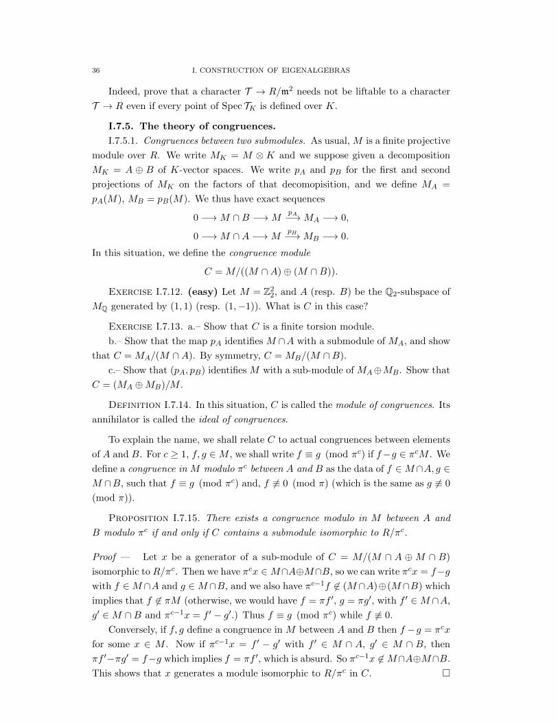
I.7.5. The theory of congruences.
I.7.5.1. Congruences between two submodules. As usual, M is a finite projective
module over R. We write MK = M ⊗ K and we suppose given a decomposition
MK = A ⊕ B of K-vector spaces. We write pA and pB for the first and second
projections of MK on the factors of that decomopisition, and we define MA =
pA(M), MB = pB(M). We thus have exact sequences
0 −→M ∩B −→MpA−→MA −→ 0,
0 −→M ∩A −→MpB−→MB −→ 0.
In this situation, we define the congruence module
C = M/((M ∩A)⊕ (M ∩B)).
Exercise I.7.12. (easy) Let M = Z22, and A (resp. B) be the Q2-subspace of
MQ generated by (1, 1) (resp. (1,−1)). What is C in this case?
Exercise I.7.13. a.– Show that C is a finite torsion module.
b.– Show that the map pA identifies M ∩A with a submodule of MA, and show
that C = MA/(M ∩A). By symmetry, C = MB/(M ∩B).
c.– Show that (pA, pB) identifies M with a sub-module of MA⊕MB. Show that
C = (MA ⊕MB)/M .
Definition I.7.14. In this situation, C is called the module of congruences. Its
annihilator is called the ideal of congruences.
To explain the name, we shall relate C to actual congruences between elements
of A and B. For c ≥ 1, f, g ∈M , we shall write f ≡ g (mod πc) if f−g ∈ πcM . We
define a congruence in M modulo πc between A and B as the data of f ∈M∩A, g ∈M ∩B, such that f ≡ g (mod πc) and, f 6≡ 0 (mod π) (which is the same as g 6≡ 0
(mod π)).
Proposition I.7.15. There exists a congruence modulo in M between A and
B modulo πc if and only if C contains a submodule isomorphic to R/πc.
Proof — Let x be a generator of a sub-module of C = M/(M ∩ A ⊕M ∩ B)
isomorphic to R/πc. Then we have πcx ∈M∩A⊕M∩B, so we can write πcx = f−gwith f ∈M ∩A and g ∈M ∩B, and we also have πc−1f 6∈ (M ∩A)⊕(M ∩B) which
implies that f 6∈ πM (otherwise, we would have f = πf ′, g = πg′, with f ′ ∈M ∩A,
g′ ∈M ∩B and πc−1x = f ′ − g′.) Thus f ≡ g (mod πc) while f 6≡ 0.
Conversely, if f, g define a congruence in M between A and B then f −g = πcx
for some x ∈ M . Now if πc−1x = f ′ − g′ with f ′ ∈ M ∩ A, g′ ∈ M ∩ B, then
πf ′−πg′ = f−g which implies f = πf ′, which is absurd. So πc−1x 6∈M∩A⊕M∩B.
This shows that x generates a module isomorphic to R/πc in C.
I.7. EIGENALGEBRAS OVER DISCRETE VALUATION RINGS 37
In other words, the ideal of congruences is the maximal ideal modulo which
there are congruences between A and B.
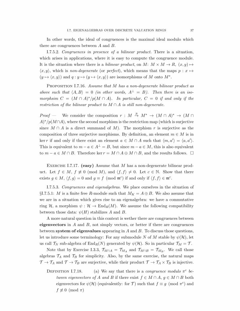
I.7.5.2. Congruences in presence of a bilinear product. There is a situation,
which arises in applications, where it is easy to compute the congruence module.
It is the situation where there is a bilinear product, on M : M ×M → R, (x, y) 7→〈x, y〉, which is non-degenerate (or perfect), which means that the maps p : x 7→(y 7→ 〈x, y〉) and q : y 7→ (y 7→ 〈x, y〉) are isomorphisms of M onto M∗.
Proposition I.7.16. Assume that M has a non-degenerate bilinear product as
above such that 〈A,B〉 = 0 (in other words, A⊥ = B). Then there is an iso-
morphsim C = (M ∩ A)∗/p(M ∩ A). In particular, C = 0 if and only if the
restriction of the bilinear product to M ∩A is still non-degenerate.
Proof — We consider the composition r : Mp→ M∗ → (M ∩ A)∗ → (M ∩
A)∗/p(M∩A), where the second morphism is the restriction map (which is surjective
since M ∩ A is a direct summand of M). The morphism r is surjective as the
composition of three surjective morphisms. By definition, an element m ∈M is in
ker r if and only if there exist an element a ∈ M ∩ A such that 〈m, a′〉 = 〈a, a′〉.This is equivalent to m− a ∈ A⊥ = B, but since m− a ∈M , this is also equivalent
to m− a ∈M ∩B. Therefore ker r = M ∩A⊕M ∩B, and the results follows.
Exercise I.7.17. (easy) Assume that M has a non-degenerate bilinear prod-
uct. Let f ∈ M , f 6≡ 0 (mod M), and 〈f, f〉 6= 0. Let c ∈ N. Show that there
exists g ∈M , 〈f, g〉 = 0 and g ≡ f (mod mc) if and only if 〈f, f〉 ∈ mc.
I.7.5.3. Congruences and eigenalgebras. We place ourselves in the situation of
§I.7.5.1: M is a finite free R-module such that MK = A⊕B. We also assume that
we are in a situation which gives rise to an eigenalgebra: we have a commutative
ring H, a morphism ψ : H → EndR(M). We assume the following compatibility
between those data: ψ(H) stabilizes A and B.
A more natural question in this context is wether there are congruences between
eigenvectors in A and B, not simply vectors, or better if there are congruences
between system of eigenvalues appearing in A and B. To discuss those questions,
let us introduce some terminology: For any submodule N of M stable by ψ(H), let
us call TN sub-algebra of EndR(N) generated by ψ(H). So in particular TM = T .
Note that by Exercise I.3.3, TM∩A = TMAand TM∩B = TMB
. We call those
algebras TA and TB for simplicity. Also, by the same exercise, the natural maps
T → TA and T → TB are surjective, while their product T → TA × TB is injective.
Definition I.7.18. (a) We say that there is a congruence modulo πc be-
tween eigenvectors of A and B if there exist f ∈M ∩A, g ∈M ∩B both
eigenvectors for ψ(H) (equivalently: for T ) such that f ≡ g (mod πc) and
f 6≡ 0 (mod π)

38 I. CONSTRUCTION OF EIGENALGEBRAS
(b) We say that there is a congruence modulo πc between system of eigenvalues
of A and B if there exists characters χA : T → TA → R and χB : T →TB → R such that χA ≡ χB (mod πc).
(c) We say that there is an eigencongruence modulo πc between A and B if
there is a character χ : T → R/πc that factors both through TA and TB.
Obviously, (a) implies (b) implies (c). However, those inclusions are strict, even
if we assume that all points of Spec TK are defined over K.
Example I.7.19. For an example of situation where (b) holds but not (a), let
R = Zp, K = Qp M = Z2p, MK = Q2
p, A = Qpe1, B = Qpe2 where (e1, e2)
is the standard basis of Z2p, and let T ∈ EndR(M) be the matrix
Ç0 00 p
å. Then
e1 and e2 are eigevectors for T of eigenvalues 0 and p, so there is a congruence
modulo (p) between systems of eigenvalues appearing in A and B. Yet there is
no congruences between A and B, as the M ∩ A = Zpe1, M ∩ B = Zpe2, so
M = (M ∩ A)⊕ (M ∩B) and the module of congruence C is trivial. Note that in
this situation the eigenalgebra T is Zp[X]/X(X − p), X acting on M by T . This
algebra T is naturally isomorphic as a Zp-algebra to (a, b) ∈ Z2p, a ≡ b (mod p),
the isomorphism sendind P (X) to (P (0), P (p)). The algebras TA and TB are just
Zp and the map T 7→ TA × TB is just the obvious inclusion T ⊂ Z2p (obvious in
terms of the second description of T ).
Exercise I.7.20. Give an example of situation where (c) holds but not (b),
even if all points of Spec TK are defined over K.
Exercise I.7.21. (easy) Show that when all points Spec TK are defined over
K, any eigencongruence modulo m between A and B comes form a congruence
between system of eigenvalues appearing in A and B. (N.B. we are talking here of
congruence modulo m, not mc.)
Among the three notions of congruences that we define, the notion (b) of congru-
ences between system of eigenvalues is the most natural and useful. Unfortunately,
it is also the more difficult to detect. Let us just mention the following easy but
weak result:
Exercise I.7.22. Assume that dimK A = 1 and that all points Spec TK are
defined over K. If the module of congruence C is not trivial, show that there is a
congruence modulo m between system of eigenvalues appearing in A and B. Show
that the converse is false.
It is relatively easy, however, to detect eigencongruences. But for that we need
a better tool than the ideal of congruence, whose definition does not take into
account the action of H on M .
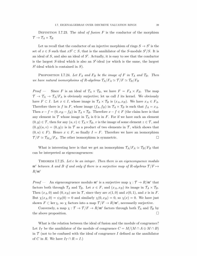
I.7. EIGENALGEBRAS OVER DISCRETE VALUATION RINGS 39
Definition I.7.23. The ideal of fusion F is the conductor of the morphism
T → TA × TB
Let us recall that the conductor of an injective morphism of rings S → S′ is the
set of x ∈ S such that xS′ ⊂ S, that is the annihilator of the S-module S′/S. It is
an ideal of S, and also an ideal of S′. Actually, it is easy to see that the conductor
is the largest S-ideal which is also an S′-ideal (or which is the same, the largest
S′-ideal which is contained in S).
Proposition I.7.24. Let FA and FB be the image of F in TA and TB. Then
we have natural isomorphsims of R-algebras TA/FA ' T /F ' TB/FB
Proof — Since F is an ideal of TA × TB, we have F = FA × FB. The map
T → TA → TA/FA is obviously surjective; let us call I its kernel. We obviously
have F ⊂ I. Let x ∈ I, whose image in TA × TB is (xA, xB). We have xA ∈ FA.
Therefore there is f in F , whose image (fA, fB) in TA × TB is such that fA = xA.
Then x− f = (0, xB − fB) in TA×TB. Therefore x− f ∈ F (the claim here is that
any element in T whose image in TA is 0 is in F . For if we have such an element
(0, y) ∈ T , then for any (u, v) ∈ TA×TB, v is the image of some element z ∈ T , and
(0, y)(u, v) = (0, y)z is in T as a product of two elements in T , which shows that
(0, u) ∈ F ). Hence x ∈ F , so finally I = F . Therefore we have an isomorphism
T /F ' TMA/FA. The other isomorphism is symmetric.
What is interesting here is that we get an isomorphism TA/FA ' TB/FB that
can be interpreted as eigencongruences:
Theorem I.7.25. Let c be an integer. Then there is an eigenconguence modulo
mc between A and B if and only if there is a surjective map of R-algebras T /F 7→R/mc
Proof — An eigencongruence modulo mc is a surjective map χ : T → R/mc that
factors both through TA and TB. Let x ∈ F , and (xA, xB) its image in TA × TB.
Then (xA, 0) and (0, xB) are in T , since they are x(1, 0) and x(0, 1), and x is in F .
But χ(xA, 0) = ψB(0) = 0 and similarly χ(0, xB) = 0, so χ(x) = 0. We have just
shown F ⊂ kerχ, so χ factors into a map T /F → R/mc, necessarily surjective.
Conversely, a map χ : T → T /F → R/mc factors through both TA and TB by
the above proposition.
What is the relation between the ideal of fusion and the module of congruence?
Let IT be the annihilator of the module of congruence C = M/(M ∩ A⊕M ∩ B)
in T (not to be confused with the ideal of congruence I defined as the annihilator
of C in R. We have IT ∩R = I.)

40 I. CONSTRUCTION OF EIGENALGEBRAS
Theorem I.7.26. We have an inclusion F ⊂ IT . If there exists a non-degenerate
bilinear product T ×M → R satisfying 〈TT ′, f〉 = 〈T ′, T f〉 for all T, T ′ ∈ T , f ∈M ,
then we have F = IT .
Proof — By definition, IT is the set of T ∈ T such that T ((M ∩ A) ⊕ (M ∩ B)
is in M . So IT = T ∈ T , T (TA × TB)M ⊂M since clrarly, (M ∩A)⊕ (M ∩B) is
generated by M as a (TA × TB)-module. So
IT = T ∈ T , T (TA × TB) ⊂ OM
where OM = (TA, TB) ∈ TA × TB, (TA, TB)M ⊂M. On the other hand,
F = T ∈ T , T (TA × TB) ⊂ T
Therefore, the inclusion F ⊂ IT follows from the trivial inclusion T ⊂ OM , which
proves the first half of the theorem.
Similarly, F = IT would follow from T = OM which we shall prove assuming
the existence of a bilinear product as in the statement. First, because of the perfect
pairing dimK TK = dimKMK , and similarly dimK TA = dimK A and dimK TB =
dimK B because the pairing induces a perfect pairing between TA ⊗K and A, and
TB ⊗ K and B. It follows that the map T → TA × TB becomes an isomorphism
after tensorizing by K. The pairing extends to a pairing TK ×MK → K, and the
non-degeneracy of the pairing means that for T ∈ TK , we have T ∈ T if and only
if 〈T, f〉 ∈ R for all f ∈ M . If T ∈ OM ∈ TA × TB ⊂ TK , and f ∈ M , we have
〈T, f〉 = 〈1, T f〉 which is in R since Tf ∈ M by definition of OM . Hence T ∈ Tand OM = T .
Exercise I.7.27. Prove that if we release the hypothesis that the pairing is non-
degenerate in the above theorem, but we assume instead that it has discriminant
of valuation c ∈ N, then IT /F is killed by πc.
I.8. Modular forms with integral coefficients
Let w ≥ 0 be an integer (the weight). Recall that the Z-submoduleMw(Γ1(N),Z)
of Mw(Γ1(N),Q) (same statement with Sw) with integral coefficients is a lat-
tice. So we can extend the preceding definitions by setting Mw(Γ1(N), R) =
Mw(Γ1(N),Z)⊗Z R for any commutative ring R. The same holds for Sw.
We now fix a prime number p, a finite extension K of Qp, of ring of integers
R. As above, m is the maximal ideal of R, and k = R/m. We consider the module
Sw(Γ1(N), R) and the eigenalgebras TR, T0,R of H, H0 acting on this module.
Similarly, we define the eigenalgebras TK , T0,K , and Tk, T0,k for the action of H,
H0 on Sw(Γ1(N),K) and Sw(Γ1(N), k).
We let Tk be the eigenalgebras generated by all Hecke operators on Sw(Γ1(N), k).
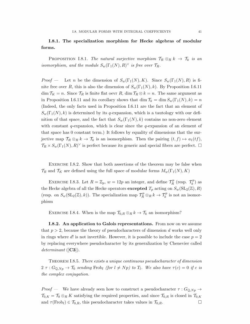
I.8. MODULAR FORMS WITH INTEGRAL COEFFICIENTS 41
I.8.1. The specialization morphism for Hecke algebras of modular
forms.
Proposition I.8.1. The natural surjective morphism TR ⊗R k → Tk is an
isomorphism, and the module Sw(Γ1(N), R)∨ is free over TR.
Proof — Let n be the dimension of Sw(Γ1(N),K). Since Sw(Γ1(N), R) is fi-
nite free over R, this is also the dimension of Sw(Γ1(N), k). By Proposition I.6.11
dim TK = n. Since TR is finite flat oevr R, dim TR ⊗ k = n. The same argument as
in Proposition I.6.11 and its corollary shows that dim Tk = dimSw(Γ1(N), k) = n
(Indeed, the only facts used in Proposition I.6.11 are the fact that an element of
Sw(Γ1(N), k) is determined by its q-expansion, which is a tautology with our defi-
nition of that space, and the fact that Sw(Γ1(N), k) contains no non-zero element
with constant q-expansion, which is clear since the q-expansion of an element of
that space has 0 constant term.) It follows by equality of dimensions that the sur-
jective map TR ⊗R k → Tk is an isomorphism. Then the pairing (t, f) 7→ a1(tf),
TR × Sw(Γ1(N), R)∨ is perfect because its generic and special fibers are perfect.
Exercise I.8.2. Show that both assertions of the theorem may be false when
TR and TK are defined using the full space of modular forms Mw(Γ1(N),K)
Exercise I.8.3. Let R = Zp, w = 12p an integer, and define T pR (resp. T pk ) as
the Hecke algebra of all the Hecke operators excepted Tp acting on Sw(SL2(Z), R)
(resp. on Sw(SL2(Z), k)). The specialization map T pR ⊗R k → Tpk is not an isomor-
phism
Exercise I.8.4. When is the map T0,R ⊗R k → Tk an isomorphism?
I.8.2. An application to Galois representations. From now on we assume
that p > 2, because the theory of pseudocharacters of dimension d works well only
in rings where d! is not invertible. However, it is possible to include the case p = 2
by replacing everywhere pseudocharacter by its generalization by Chenevier called
determinant ([C3]).
Theorem I.8.5. There exists a unique continuous pseudocharacter of dimension
2 τ : GQ,Np → T0 sending Frobl (for l 6= Np) to Tl. We also have τ(c) = 0 if c is
the complex conjugation.
Proof — We have already seen how to construct a pseudocharacter τ : GQ,Np →T0,K = T0 ⊗R K satisfying the required properties, and since T0,R is closed in T0,K
and τ(Frobl) ∈ T0,R, this pseudocharacter takes values in T0,R.
42 I. CONSTRUCTION OF EIGENALGEBRAS
Thus we have glued all the Galois representations attached to eigenforms in
Mk(Γ1(N)) in one unique pseudocharacter, with values in the algebra T0,R.
Let us give one application.
Corollary I.8.6. Let n ≥ 1 be an integer, f ∈Mk(Γ1(N), ε, R) be a normalized
form such that for every prime l not dividing Np, Tlf ≡ χ(Tl)f (mod mn) where
χ(T ) is some element in R/mn. There exists a pseudocharacter τf : GQ,Np → R/mn
such that τ(Frobl) = χ(Tl) in R/mn.
So we can attach Galois pseudocharacters not only to true eigenforms, but
more generally to eigenform modulo mn. Of course the pseudocharacter we get
takes values in R/mn instead of R.
Had we not the above theorem, the obvious method to prove the result of the
corollary would be to replace f by a true eigenform g with eigenvalues congruent
to the χ(Tl) modulo mn. Then the would reduce the Eichler-Shimura-Deligne rep-
resentations ρg modulo mn and take the trace. The Deligne-Serre’s lemma tells us
that we can find such a g when n = 1, but in general we cannot. So this approach
fails. Yet with what we have done, the proof of the corollary is trivial:
Proof — Since f is normalized, the element χ(Tl) of R/mn depends only on Tl ∈T0,R, hence χ extends to a character T0,R → R/mn. Composing τ : GQ,Np → T0,R
of the above theorem with χ gives the result.
The drawback of the corollary is that, attached to a modular forms which is an
eigenform mofulo mn, we get only a pseudocharacter valued in R/mn, not a true
representation. However, there are many results saying that a pseudocharacter
is, in many circumstances, the trace of a representation. Let us recall the most
improtant ones: If T : G → k is a pseudocharacter of dimension d valued in an
algebraically closed field k, then T comes form the trace of a unique semi-simple
representation G → GLd(k). This is a theorem of Taylor [T] and Rouquier [Ro].
And if T : G→ A is a pseudocharacter of dimension d valued in an henselian local
ring with residue field k, so that the residual pseudocharacter T : G → k is the
trace of an absolutely irreducible representation G → GLd(k), then T is the trace
of a unique representation G → Gld(A). This is a theorem of Rouquier [Ro] and
Nyssen [Ny].
For any maximal ideals mi of T0, the quotient ki := T0/mi is a finite field, so
the pseudocharacter τmi : GQ,Np → T0 → T0/mi = ki is the trace of a unique
semi-simple representation ρmi : GQp : GQ,Np → GL2(ki) by the theorem of Taylor
and Rouquier. Actually ρmi is defined over ki (there are many ways to see it: the
simplest is too observe that ρi(c) has distinct eigenvalues).
We call the maximal ideal mi of T0 (or their connected component in Spec T0)
non-Eisenstein if ρmi is absolutely irreducible, and Eisenstein otherwise.

I.9. A COMPARISON THEOREM 43
Theorem I.8.7. Let Spec T0,mi be a non-Eisenstein component. There exists a
unique Galois representation ρmi : GQ,Np → GL2(T0,mi) such that tr ρmi(Frobl) = Tl
in T0,mi.
Indeed, the condition on the trace means that tr ρmi is the pseudocharacter
τmi : GQ,Np → T0 → T0,mi . The residual pseudocharacter is, by assumption, the
trace of an absolutely irreducible representation. The result follows from the thorem
Rouquier-Nyssen.
The fact that we have a true representation over T0,mi (assume this component
non-Eisenstein) allows us to make a comparison with Mazur’s deformation theory.
Let Rmi be the universal deformation ring of the residual representation ρmi :
GQ,Np → GL2(ki). SInce T0,mi is a coefficient ring (that is complete local noetherian
of residue field ki), and since ρmi obviously deforms ρmi , there is a morphism of
coefficient rings
Rmi → T0,mi
which sends the universal deformation representation on Rmi to ρmi .
Exercise I.8.8. Show that the map Rmi → T0,mi is surjective.
The remarkable idea of Wiles leading to the proof of the Shimura-Taniyama-
Weil conjecture in the semi-stable case (hence of Fermat’s last theorem) was a
method to determine the kernel of this map in simple cases (weight k = 2, and ρmiof a very special type). This method has then been generalized to many more cases,
leading to the proof of the Shimura-Taniyama-Weil conjecture in general, and even
of the Fontaine-Mazur conjecture in many cases.
I.9. A comparison theorem
In this §, we only assume that R is noetherian and reduced. For every point
x ∈ Spec (R), of field k(x), we callMx = M⊗Rk(x) and Tx the subalgebra generated
by ψ(H) in Endk(x)(Mx).
Lemma I.9.1. Assume that for x in a Zariski-dense subset Z in SpecR, H acts
semi-simply on Mx. Then T is reduced.
Proof — The hypothesis implies that for x ∈ Z, Tx is reduced.
Let t ∈ T such that tn = 0 for some n ≥ 1. Let tx be the image of t by the
natural map EndR(M) → Endk(x)(Mx). We have tnx = 0, so for x ∈ Z, we get
tx = 0.
If M is free over R, that means that every matrix element of t ∈ EndR(M) is
0 at every x ∈ Z. Since Z is dense and R is reduced, evert matrix element of t is 0
period, and t = 0.
In the general case, M is projective, so N = M⊕Q say is free. Apply the result
in the free case to the endomorphism t′ of N such that t′|M = t, t′|Q = 0.
44 I. CONSTRUCTION OF EIGENALGEBRAS
Now let us assume that M and M ′ are two finite projective R-modules with
action ψ and ψ′ of H, and let T and T ′ be there associated algebras.
Theorem I.9.2. Let us assume that for every x in a Zariski-dense subset Z of
R, Mx is a semi-simple H-module, and there is an H-injection M ′x ⊂ Mx. Then
there is a canonical surjection T → T ′ (that is, a closed immersion Spec T ′ ⊂Spec T ). Moreover, for every x ∈ SpecR, there is an H-injection (M ′x)ss → (Mx)ss
Proof — Let t ∈ H ⊗ R. Let Pt(X), P ′t(X) in R[X] be the characteristic poly-
nomials of ψ(t) and ψ′(t). If x ∈ SpecR, let Pt,x(X) and P ′t,x(X) be the images
of those polynomial in k(x)[X]. They are also the characteristic polynomials of
ψ⊗1(t) and ψ′⊗1(t) in Endk(x)(Mx), Endk(x)(M′x). By hypothesis, for x ∈ Z, P ′t,x
divides Pt,x in k(x)[X] for x ∈ Z. As Z is dense, Pt divides P ′t in R[X], from which
it follows that Pt,x|P ′t,x for every x ∈ SpecR. By elementary representation theory,
this proves the second assertion.
For the second assertion, we can work locally and assume that M is free of
rank d. By the lemma, T and T ′ are reduced. Let us call J (resp. J ′) the kernel
J of ψ : H⊗R → EndR(M) (resp. ψ′ : H ⊗ R → EndR(M ′)). If t ∈ J , ψ(t) = 0
so Pt = Xd. So P ′t |Xd, and by Calley-Hamilton ψ(t′)d = 0, so ψ(t′) = 0. Hence
J ⊂ J ′ and the theorem follows.
Corollary I.9.3. Let us assume that for every x in a Zariski-dense subset Z
of R, Mx is a semi-simple H-module, and there is an H-isomorphism M ′x ' Mx.
Then there is a canonical isomorphism T = T ′. Moreover, for every x ∈ SpecR,
there is an H-isomorphism (M ′x)ss ' (Mx)ss
I.10. Notes and References
In a sense, the idea, in the context of Hecke operators acting on spaces or
modules of modular forms, of conisdering the sub-algebra of the endomorphism
algebra of that space and moduel generated by those operators – that we call the
eigenalgebra here – is so tautological that it is impossible to trace back its origin: as
soon as we consider operators acting on a space or module, we implicitly or explicitly
consider the subalgebra they generate. Yet the realization that this eigenalgebra
was an important object, even perhaps the central object on the theory, that the
algebraic properties of this commutative algebra (which by Grothendieck’s theory
of schemes can be reformulated into geometric properties of its spectrum) were a
way to express and study the properties of eigenforms, this reaization I say was
long to come, and a fundamental progress when it did.
Over a field (a subfield of C), this idea certainly occured to Shimura3, which
defines and prove some elementary properties in his book [Shi]. He for example
3perhaps even earlier. Eichler? Selberg? If anyone has any information on that -or in general,this history, please contact me.
I.10. NOTES AND REFERENCES 45
raised the following question: is the eigenalgebras T generated by all the Hecke
operators acting on the space S2(Γ0(N),Q) isomorphic to the algebras of isogenies
of the modular Jacobian J0(N). This question was solved affirmatively by Ribet
[Ri] in 1975.
Over a ring like the ring of integers of a number field, or a localization or
completion of such a ring, the study of the eigenalgebra is intimely related to the
study of the arithmetic property of modular forms. The eigenalgebra appears in
[De], in the second proof of the famous Deligne-Serre’s lemma, but it seems that
Mazur was the first to study and use the algebraico-geometric propertoes of those
eigenalgebras, in its very influential 1978’s paper [Mazur], to prove deep arithmetic
results about modular forms and elliptic curves. Most of the important progresses
in the arithmetic theory of modular forms ever since have used and developped
that very idea (often named Hecke algebras). To mention a few of them: uses
of the Hecke algebras to study congruences between modular forms ([H1], [H2],
[Ri2]), use of big Hecke Algebra (Eigenalgebra over Iwasawa’s algbra) by Hida to
construct the first p-adic modular forms, use of those Hecke algebra to prove the
main conjetcures ([MaW], [W]), use of eigenalgebras (and their fine algebraico-
geometric properties) in the proof of Fermat’s last theorem ([W], [TW]), and use
of new kind of ”big Hecke algebras” by Coleman ([Col2] to construct non-ordinary
families of modular forms, and more generally by Coleman-Mazur [CM] and other
to construct the eigencurve or eigenvarieties (also called varieties of Hecke).
In this chapter, we have tried to expose the formal aspects of the construction
of eigenalgebras, relying on the work of the aforementioned mathematicians and
many other. We know try to give a proper attribution to most of the results that
are not standard commutative algebra.
In §I.1, §I.2 and §I.3, almost all results are elementary. Exercise I.3.6 is due to
Buzzard. Prop. is due to G. Chenevier ([C1]).
Prop. I.4.1 is due to G. Chenevier ([C1]), at lest in the case of a surjective map
R→ R′.
The results of §I.5 are essentially linear algebras, and commutative linear alge-
bra.
Most of the results of §I.6 are due to Shimura ([Shi]) though the emphasis on
the notion of Gorensteinness in this context seems due to Mazur.
As for eigenalgebras over a base ring which is a D.V.R. (or more generally a
Dedekind domain), as we said they appear in [De], and [Mazur]. The interpre-
tation of those maximal and prime ideals as eigenforms, etc. given in ??, which
is again elementary commutative algebra, is sketched in a few sentences in [De].
Each subsequent author stated the part he needed, until all those things became
completely standard at the time of the proof of Fermat’s Last Theorem – The sur-
vey [DDT] contains an exposition of that theory, which also mention the link with
46 I. CONSTRUCTION OF EIGENALGEBRAS
Deligne-Serre’s lemma. The theory of congruences exposed in §I.7.5 is essentially
due to Hida (e.g. [H1], [H2] and Ribet (e.g. [Ri2])). A good survey is [Gh].
The results of §I.9 are due to Chenevier ([C2]).
CHAPTER II
The Eigenvariety Machine
In this chapter, we explain the construction of eigenvarieties, which is a version
at large and in a rigid analytic setting of the construction of eigenalgebras of the
previous chapter. We shall not be entirely self-contained for the proofs: the reason
is that there is already a very good text explaining the construction of the eigen-
varieties, Buzzard’s paper [Bu]. However we hope that our exposition will allow
a reader willing to either admit or look up in [Bu] the proofs of a few important
technical results along the way, to get a working understanding of what an eigenva-
riety is and how it is constructed. We also want to improve somewhat on Buzzard’s
construction by giving a more precise control on the local pieces that are glued to
construct the eigenvarieties.
Compared with the setting of a construction of an eigenalgebra of the preceding
chapter (a base ring R, a finite flat R-module M , a morphism ψ : H → EndR(M)
where H is some commutative ring of Hecke operators), the setting of eigenvarieties
is enlarged in two directions. The base ring R, or rather its spectrum SpecR is
replaced by a rigid analytic variety W, which will not be an affinoid in general.
Hence it would be natural to replace M by a coherent locally-free sheaf over W,
but here comes a second, more important, enlargment: we want to replace the
finite module M by a non-finite Banach module. To avoid talking of sheaf of Banach
modules (which we could, as in [CM] or [C2]), we simply define our data as in [Bu]
by the giving, for every affinoid subdomain W = SpR of W, of a Banach-module
MW over R (satisfying some technical condition of orthonormability), provided
with an action of the ring H. The modules MW for various W are required to
satisfy some compatibility relations, that are explained in section §II.2. To deal
with the new infiniteness of our module, we introduce a crucial hypothesis: that
our ring H contains a privileged element Up ∈ H that acts compactly on the various
Banach modules MW .
From those data, our aim is to construct in a canonical way an eigenvariety E ,
that is a rigid analytic variety together with a locally finite map κ : E → W, and a
morphism of rings ψ : H → O(E) allowing us to see element of H as functions on
E . The eigenvariety should have the fundamental property that its points z (over
a given point w ∈W ) classifies the system of H-eigenvalues appearing in the fiber
Mw of the modules MW at w (that fiber does not depend on the chosen affinoid
W of W containing w) that are of finite slope, that is for which Up has a non-zero
47

48 II. THE EIGENVARIETY MACHINE
eigenvalue. The bijection should be naturally given as follows: to a point z should
correspond the system of eigenvalues T 7→ ψ(T )(z), for any T ∈ H.
In order to construct the eigenvariety, we glue some local pieces that are rigid
analytic spectrum of eigenalgebras constructed as in the precideing chapter. More
precisely, if W = SpR is an admissible affinoid subdomain of W, and ν is a real
number, it is often (but not always!) possible to define in a natural way a finite
flat direct summand R-sumboldue M≤νW of MW which is morally the ”slope less or
equal to ν” part of MW , that is the submodules of vectors on which Up acts with
generalized eigenvalues of valuation lest or equal than ν. When this is possible, we
say that W and ν are adapted. Those notions are explained in our first section II.1,
which also proves that there are enough, in some precise sense, pairs (W, ν) that
are adapted.
In section §II.3.2, we explain our variant of [Bu]’s eigenvariety machine, con-
structing the eigenvariety by gluing the spectrum of eigenalgebras TW,ν defined by
the action of H on M≤νW for adpated pair (W, ν).
In section II.4 we list the most important properties of the eigenvarieties, due
to Coleman-Mazur ([CM]) or Chenevier ([C1]), in particular we explain why their
points parametrize system of eigenvalues of finite slope.
In the last section II.5 we explain and prove a very useful result of Chenevier
(cf. [C2]) allowing to compare two eigenvarieties.
II.1. Submodules of slope ≤ ν
Let L be a finite extension of Qp, R be a reduced affinoid algebra over L,
that we provide with its supremum norm | | extending the norm of L (which itself
extends the standard p-adic norm on Qp). We set as usual vp(x) = − log |x|/ log p,
so vp(p) = 1.
Let us call RT the ring of power series∑∞n=0 anT
n, with an ∈ R, that
converge everywhere, that is such that vp(an)− nν →∞ for every ν ∈ R.
Definition II.1.1. Let F (T ) ∈ RT, and ν ∈ R. We write N(F, ν) for the
largest integer n such that vp(an)− nν = infm(vp(am)−mν).
Exercise II.1.2. (easy) Prove Gauss’ lemma: N(FG, ν) = N(F, ν)N(G, ν).
Exercise II.1.3. If F (T ) ∈ LT, and ν ∈ R, then N(F, ν) is the number of
zeros z in L of F (T ) with vp(z) ≥ −ν, counted with multiplicity.
If x ∈ SpR is a closed point of field of definition L(x), we write Fx(T ) for the
series∑∞n=0 an(x)Tn which belongs to L(x)T.
Exercise II.1.4. (easy) If N(Fx, ν) is a constant N independent of x ∈ SpR,
then N(F, ν) = N .
Definition II.1.5. A polynomial Q(T ) ∈ R[T ] is called ν-dominant if

II.1. SUBMODULES OF SLOPE ≤ ν 49
(i) Q has degree N(Q, ν)
(ii) For all x ∈ SpecR, N(Q, ν) = N(Qx, ν)
Note that if a polynomial Q(T ) ∈ R[T ] is ν-dominant, then its dominant term
aN(Q,ν) is invertible in R. For if it was not, aN(Q,ν)(x) would be zero for some x,
and we would have N(Qx, ν) ≤ degQx < degQ = N(Q, ν).
Exercise II.1.6. Let Q be a polynomial satsifying (i) of the definition of ν-
dominant. Assume that aN(Q,ν) is invertible, and that |aN(Q,ν)||a−1N(Q,ν)| = 1. Show
that Q is ν-dominant.
Fix an F ∈ RT and assume F (0) = 1. As in [Bu, §4], let us write
W = SpR, and let Z be the analytic subvariety of W × A1rig cut out by F (T ),
where A1rig is the rigid analytic affine line over L. Let f be the projection map
Z →W , and let Zν be the affinoid of Z of points z whose component in A1rig have
vp(z) ≥ −ν. Then the Zν are quasi-finite over W according to Exercise II.1.3, and
it is not hard to see that they are also flat (cf. [Bu, Lemma 4.1]).
Proposition II.1.7. For F (T ) ∈ RT with F (0) = 1, and ν ∈ R, the
following are equivalent:
(i) The map f : Zν →W is finite.
(ii) There exists a decomposition F = QG in RT, with Q(0) = G(0) = 1,
where Q is a ν-dominant polynomial of degree N(F, ν).
(iii) One has N(Fx, ν) = N(F, ν) for all x ∈W ,
If those properties hold, the decomposition F = QG as in (ii) is unique, (Q,G) = 1
in RT, Zν is disconnected from its complement in Z (that is, there is an
idempotent e ∈ O(Z) such that Z is defined by e = 1) and f : Zν → B is finite flat
surjective of degree degQ = N(F, ν).
Proof — Assume (i). Then f : Zν → W , which is always flat, is also surjective.
Moreover Zν is disconnected from its complement Z ′ ⊂ Z, since by [BGR, 9.6.3/3
and 9.5.3/5], Z ′ ⊂ Z is both an open and a closed immersion. The finite flat R-
algebra O(Zν) is generated by the function t ∈ O(Zν) defined by the natural map
Zν → A1. Let Q ∈ R[T ] be the characteristic polynomial of the multiplication by t
on O(Zν). Then the natural surjective morphism T 7→ t, R[T ]/Q(T )→ O(Zν) is an
isomorphism be equality of rank. Hence we get a factorization F = QG, with G ∈RT whose zero locus is Z ′. For x ∈W , we have a decomposition Fx = QxGx,
and the zeros of Qx are exactly the zeros of Fx in Zν , that is such that vp(x) ≥ −ν.
It follows that N(Fx, ν) = N(Qx, ν) = degQx = degQ. Therefore Q is ν-dominant
of degree N(F, ν) (exercise II.1.4). Moreover since 1 = F (0) = Q(0)G(0) we can
divides Q by Q(0) and assume that Q(0) = G(0) = 1 and we have a decomposition
(ii), and (iii) holds.

50 II. THE EIGENVARIETY MACHINE
Conversely, given a decomposition (ii), then the locus Q = 0 is finite over W
(remember that the dominant term of Q is invertible), and we easily see it is Zν .
Also, if (iii) holds, then the fibers of f : Zν → W all have the same degrees
N(F, ν). Thus f is finite by [Bu, Corollary 4.3], and (i) holds.
So we have proven the equivalence of (i), (ii) and (iii), and that when they hold
Zν is disconnected from its complement Z ′. It follows that (Q,R) = 1 in RT.The uniqueness of the decomposition F = QR follows from the proof since the map
T 7→ t, R[T ]/Q(T ) → O(Zν) has to be an isomorphism, which characterizes Q up
to an invertible element in R, and that element is fixed by the condition Q(0) = 0.
Definition II.1.8. A power series F (T ) ∈ RT with F (0) = 1 being fixed,
we say that ν ∈ R is adapted to F if the conditions of the above proposition are
satisfied.
The main interest of this notion is in the following definition and proposition.
Definition II.1.9. LetM be a Banach R-module satisfying property (Pr) ([Bu,
§2]), and Up a compact R-linear operator of M (loc. cit.). Let F (T ) ∈ RT be
the Fredholm power series of Up (that is F (T ) = det(1−TUp) loc. cit.). If ν ∈ R is
adapted for F , we write M≤ν for the kernel of the operator Q∗(Up), where Q is the
polynomial appearing in the decomposition of F in (ii) of the above proposition,
and Q∗ is its reciprocal polynomial, and we call M≤ν the submodule of M of slope
less than ν.
Proposition II.1.10. If ν is adapted for F (T ), then M≤ν is a finite flat mod-
ule over R of rang N(F, ν). It is a direct summand of M . The formation of
M≤ν commute with base change, in the sense that if R → R′ is a morphism of
affinoid rings over L, then ν is adapted for the image of F (T ) in R′T, and
(M⊗RR′)≤ν = M≤ν ⊗R R′ as submodules of M⊗RR′.
Proof — The first sentence is [Bu, Theorem 3.3]. For the commutation with
base change, note that U ′p := Up⊗1 is a compact operator of M⊗RR′ whose
power series is the image F ′(T ) of F (T ) in R′T by [Bu, Corollaries 2.9 and
2.10]. The decomposition F = QG in RT defines a decomposition F ′ = Q′G′
which obviously still satisfies (ii) of Prop II.1.7. Hence ν is stll adapted for F ′,
and Q′∗(U ′p) = Q∗(Up)⊗1. It follows from the proof of [Bu, Theorem 3.3] that
(M⊗RR′)≤ν = M≤ν ⊗R R′.
Remark II.1.11. By its definition as the kernel of a polynomial in Up, the
submodule M≤ν of M is stable by any endomorphism of M that commutes with
Up.
II.2. LINKS 51
For X an affinoid open of W , of affinoid ring RX , we call FX(T ) the image
of F (T ) in RXT, and define ZX = f−1(X). Clearly ZX is also the analytic
subvariety in X ×A1rig cut by FX . We shall say that ν is adapted to X (or that X
and ν are adapted) if ν is adapted to FX . In this case ZX,ν := ZX ∩ Zν is finite
flat surjective over X, and we have a decomposition FX(T ) = QX(T )GX(T ) in
RXT as in Prop. II.1.7.
Of course, this notion is useful only if we can prove that there are enough
adpated (X, ν).
Proposition II.1.12. For any real ν, and any x ∈W , there exists an admissible
affinoid neighborhood X of x such that (X, ν) is adapted.
Proof — Let N = N(Fx, ν). As vp(an) − nν goes to infinity, there exist an n0
such that for all n > n0, vp(an)− nν > vp(aN (x))−Nν. Let X be the subdomain
of W such that for all n, 0 ≤ n ≤ n0, and all y ∈ X, vp(an(y)) = vp(an(x)) if
an(x) 6= 0, (resp. vp(an(y)) > vp(aN (x)) − Nν + nν if an(x) = 0). Then X is
clearly an affinoid admissible subdomain of W , and it is plain that for all y ∈ X,
N(Fy, ν) = N(Fx, ν) = N(FX , ν). Thus (X, ν) is adapted.
Corollary II.1.13. The family of affinoid subdomains ZX,ν of Z for X an
affinoid of Z and ν adapted to X is a covering of Z.
Remark II.1.14. Actually, we can show using [Bu, §5], that this family is
an admissible covering of Z. This is a slightly more precise version of the main
technical result of [Bu], namely Theorem 4.6. The covering that Buzzard considers,
C is actually larger, as it is the set of all affinoid subdomain Y of Z such that there
exists a subdomain X in W such that f(Z) = X and f : Z → X is finite. Observe
that by definition, an affinoid subdomain of Z of the form ZX,ν belongs to Buzzard’s
cover C if and only if ν is adapted to X. To check that our smaller set of affinoid
subdomains is an also admissible cover of Z, we only have to observe that all the
affinoid subdomains in C exhibited by Buzzard in order to prove his Theorem 4.6
are produced in [Bu, Lemma 4.5], and are actually (as stated in that lemma) of
the form ZX,ν .
II.2. Links
Definition II.2.1. If R is an affinoid ring, M and M ′ be two Banach R-
modules satisfying properties (Pr) with morphisms ψ : H → EndR(M) and ψ′ :
H → EndR(M ′) such that ψ(Up) and ψ′(Up) are compact, we say that M and M ′
are linked if ψ(Up) and ψ′(Up) have the same characteristic power series F (T ), and
for every monic polynomial Q ∈ R[T ] with invertible constant term, kerQ(ψ(Up))
and kerQ(ψ′(Up)) are isomorphic as R-modules with action of H.

52 II. THE EIGENVARIETY MACHINE
It is clear that to be linked is an equivalence relation. Observe that if M and
M ′ are linked, then ν is adapted from M if and only if it is adpated for M ′, and
then the two modules M≤ν and M ′≤ν are isomorphic as R-modules with action of
H.
Lemma II.2.2. Let M and M ′ be as in the definition above. Assume that there
is two continuous homomorphism of R-modules and H-modules f : M → M ′ and
g : M ′ →M such that g f = ψ(Up) and f g = ψ(U ′p). If either f or g is compact,
then M and M ′ are linked.
Proof — That the characteristic power series of ψ(Up) and ψ′(Up) are the same
results from the equality in RT: det(1− Tfg) = det(1− Tgf) proved in [Bu,
Lemma 2.12]. Moreover f maps kerQ(ψ(Up)) into kerQ(ψ′(Up)) since it is an
H-homomorphism and g maps kerQ(ψ(Up)) into kerQ(ψ(Up)). The compoistion
g f = ψ(Up) on kerQ(ψ(Up)) is invertible since Q has invertible constant term,
and so is f g. Thus kerQ(ψ(Up)) and kerQ(ψ′(Up)) are isomorphic.
An interesting special case is the following:
Lemma II.2.3. Let M,M ′ be two R-modules with H-actions as above. Assume
that there are two homomorphisms of R-modules and H-modules f : M → M ′
and g : M ′ → M such that f is injective and continuous, g is compact, and f g = ψ(U ′p). Then M and M ′ are linked. Moreover, if f factors as a composition
M →M ′′ →M ′, where M ′′ is as in the definition above and the two morphisms in
this factorization are injective continuous morphism of R-modules and H-modules,
then M and M ′ are also linked to M ′′.
Proof — For the first assertion, we observe that f g f = ψ(U ′p) f = f ψ(Up)
hence by injectivity of f , g f = ψ(Up) and we can apply Lemma II.2.2. The
second assertion follows form the first by replacing M by M ′′, f by the injection
M ′′ →M ′, and g by the composition of g : M ′ →M with the injection M →M ′′.
Lemma II.2.4. If M and M ′ are linked, and SpR′ → SpR is a morphism of
affinoid, them M⊗RR and M ′⊗RR′ are also linked.
Proof — This is clear from [Bu, Corollary 2.9]
II.3. The eigenveriety machine
II.3.1. Eigenvariety data. An eigenvariety data over a finite extension L of
Qp is the data of
(ED1) A commutative ring H, with a distinguished element Up.
II.3. THE EIGENVERIETY MACHINE 53
(ED2) A reduced rigid analytic variety W over L, and an admissible covering C
by admissible affinoid open subsets of W.
(ED3) For every admissible affinoid W = SpR of W, W ∈ C, a Banach module
MW satisfying property (Pr), and a map ψW : H → EndR(MW ).
satisfying the following conditions:
(EC1) For every W ∈ C, ψW (Up) is compact on MW .
(EC2) For every pair of affinoid subdomains W ′ = SpR′ ⊂ W = SpR ⊂ W,
W,W ′ ∈ C, the R′-Banach modules MW ⊗RR′ and MW ′ are linked (cf.
Definition II.2.1)
In (ED3) it would suffice to give the modules MW up to a link, as we will only
use construction that depends only on the link-equivalence class of MW
Given an eigenvariety data, and a closed point w ∈ W of field of definition L(w),
we can define the fiber Mw as follows: choose an affinoid admissible subdomain in C,
W = SpR, containing w, and set Mw = MW⊗RL(w), where the implicit morphism
R → L(w) is the obvious one (the evaluation at w, that is). Then the space Mw
inherits a linear action of H (ψw : H → EndL(w)(Mw)), and it is together with that
action, well defined (independent of the choice of W ) up to a link (by (ED2) and
Lemma II.2.4). In particular, the subspace of finite slope M#w of Mw defined as
M#w = ∪ν<∞M≤νw ,
is well-defined.
With no loss of generality, we can and will assume that if X ⊂W is an inclusion
of affinoid subdomain of W, with W ∈ C, then X ∈ C as well. It suffices to define
MX as MW ⊗R R′ if W = SpR and X = SpR′, which makes MX well-defined up
to a link.
II.3.2. Construction of the eigenvariety. For any admissible affinoid sub-
domain W = SpR in C, let FW ∈ RT be the characteristic power series of Up
acting on MW (that is FW (T ) = det(1 − TψW (Up)).) To any such W , and ν ∈ Radapted to W (that is, adapted to FW ), we attach a local piece of the eigencurve
which is the following:
(a) An L-affinoid variety
EW,ν = Sp TW,ν
called the local piece.
(b) A finite morphism κ : EW,ν →W called the weight map.
(c) A morphism of rings ψ : H → O(EW,ν) = TW,ν .
The construction is as follows: since ν is adapted, we can definite the finite flat
R-submodule M≤νW . Since H is commutative, it stabilizes M≤νW by Remark II.1.11.
We can therefore let TW,ν be the eigenalgebra (cf. Chapter I) of H acting on M≤νW ,
that is as the R-subalgebra of EndR(MW ) generated by ψW (H).

54 II. THE EIGENVARIETY MACHINE
Then TW,ν is a finite R-module, hence an affinoid algebra since R is, and we
define EW,ν = Sp TW,ν . The structural map defines a finite morphism of rigid affinoid
variety κ : EW,ν = Sp TW,ν → W = SpR. And we have by construction a natural
map ψ : H → TW,ν .
Lemma II.3.1. Let W ′ ⊂ W be an inclusion of admissible open affinoid of W,
with W,W ′ ∈ C. Let ν ′ ≤ ν, and assume that (W, ν) and (W ′, ν ′) are adapted.
Then there exists a unique open immersion EW ′,ν′ → EW,ν compatible with the
weight maps κ and the maps ψ from H. Its image is the affinoid open subset of
EW,ν defined by the equations vp(Up(z)) ≥ ν ′, κ(z) ∈W ′.
Proof — Note that since ν is adapted to W , it is also adapted to W ′. By
considering the intermediate (W ′, ν), we can reduce to the two cases where W = W ′
and to the case where ν = ν ′.
In the case W = W ′ = SpR, EW,ν and EW,ν′ are the Hecke algebras attached
to M≤ν and M≤ν′
respectively. But it follows from the definitions that M≤ν′
is a
sub-R-module stable by H of Mν which is a direct summand as R and H-modules
(indeed, M≤ν and M≤ν′
are defined as the kernel of Q∗(Up) and Q′∗(Up) and we
have that Q = Q′Q′′ with (Q′, Q′′) = 1 by Prop. II.1.7 applied to Q instead of F ).
Thus EW,ν is the disjoint union of EW,ν′ and its complement, and the result follows
easily in this case.
We now treat the case where W ′ = SpR′ ⊂ W = SpR but ν = ν ′. We
have (MW ⊗RR′)≤ν ' M≤νW ′ as H-modules, since MW ⊗RR′ and MW ′ are linked
by hypothesis. Therefore their eigenalgebras are isomorphic. On the other hand
we also have (MW ⊗RR′)≤ν = M≤νW ⊗R R′ by Prop. II.1.10. Then, since R′ is R-
flat, by proposition I.4.1 we see that the Hecke-algebra of M≤νW ⊗RR′ is TW,ν⊗RR′.Combining the above, we have constructed an isomorphism (obviously R-linear and
compatible with the morphisms from H):
TW,ν⊗RR′ = TW ′,ν
which shows that EE′,ν is the open affinoid of EW,ν defined by κ(z) ∈W ′.Finally, the isomorphism we have constructed is unique since the eigenalgebras
are generated by ψ(H) over R.
The eigenvariety is then constructed by gluing the local pieces:
Definition II.3.2. An eigenveriety for the above eigenvariety data, consists of
(a) A rigid analytic variety E/L (the eigenvariety proper)
(b) A locally finite map κ : E → W.
(c) A morphism of rings ψ : H → O(E), that sends Up to an invertible func-
tion.
such that for any affinoid subdomain W of W in C, and real ν adapted to W , the
open subvariety E(W, ν) of κ−1(W ) ⊂ E defined by vp(ψ(Up)) ≤ ν, is isomorphic
II.3. THE EIGENVERIETY MACHINE 55
(as analytic variety over W with a map ψ form H to their ring of functions) to the
local piece EW,ν constructed above, and such that the E(W, ν) form an admissible
covering of E .
Note that the isomorphisms E(W, ν) ' EW,ν whose existences are required by
the definition are necessarily unique.
Theorem II.3.3. For any given eigenvariety data, an eigenvariety exists and
is unique up to unique isomorphism.
Proof — We first prove the existence, by gluing, in two steps. First let W be an
open admissible affinoid of W, in C. We will construct an ’eigenvariety’ EW with
the same data and properties as E but with W always replaced by W .
We consider the family of affinoid varieties EX,ν for X ⊂ W an open affinoid
subdomain, and ν a real number adapted to X. We define a gluing data on this fam-
ily as follows: given two EX,ν and EX′,ν′ then by Lemma II.3.1 (X ∩X ′,min(ν, ν ′))
is adapted, and EX∩X′,min(ν,ν′) can be seen as an open affinoid subset of both EX,νand EX′,ν′ , in a unique way respecting the maps form H, and the weight maps.
Hence we have defined two open affinoids of EX,ν and EX′,ν′ , and an isomorphism
between them. It is clear by uniqueness that those isomorphisms satisfy the cocycle
condition. Thus, by [BGR, Prop. 9.3.2/1] we can glue the EX,ν ’s to form a rigid
analytic variety EW , of which the EX,ν ’s are an admissible covering by admissible
open affinoid subdomains. Then the maps κ : EX,ν → X glue into a single map
κ : EW → W by [BGR, Prop. 9.3.1/1]. Also the maps ψ : H → O(EX,ν) glue
into a map ψ : H → O(EW ) because the EX,ν form an admissible covering. The
uniqueness of EW up to unique isomorphism (compatible with κ and ψ) is obvious.
Finally, to construct E we have to glue the EW ’s. The only minor difficulty is
that because W is not itself an affinoid, the intersection of two admissible affinoid
subdomains W and W ′ of W may not be affinoid. But W ∩W ′ is an admissible
open subdomain and can be admissibly covered by affinoids Wi. Therefore, we can
define an isomorphism between the open admissible subdomains κ−1(W ∩W ′) in
EW and E ′W by gluing (using again [BGR, Prop. 9.3.1/1]) the isomorphism between
the κ−1(Wi) in EW and EW ′ obtained by identifying the two κ−1(Wi)’s considered
as a subdomain of EW or EW ′ obtained from identifying them to the eigenvariety
EWi . Since by uniqueness those isomorphisms obviously satisfy the gluing condition,
[BGR, Prop 9.2.1/1] and [BGR, Prop 9.3.1/1] gives us finally the eigenvariety Eby gluing the EW , with a map κ : E → W gluing the maps κ : E → W and a
morphism of rings ψ : H → O(E) gluing the morphism ψ : H → O(EW ). The
eigenvariety E with those maps obviously is unique up to unique isomorphism and
satisfies all the property stated in the theorem.
Exercise II.3.4. Prove the following easy functoriality results for eigenvarieties.
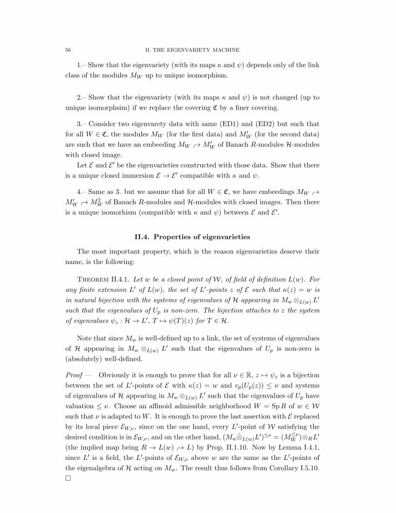
56 II. THE EIGENVARIETY MACHINE
1.– Show that the eigenvariety (with its maps κ and ψ) depends only of the link
class of the modules MW up to unique isomorphism.
2.– Show that the eigenvariety (with its maps κ and ψ) is not changed (up to
unique isomorphsim) if we replace the covering C by a finer covering.
3.– Consider two eigenvarety data with same (ED1) and (ED2) but such that
for all W ∈ C, the modules MW (for the first data) and M ′W (for the second data)
are such that we have an embeeding MW →M ′W of Banach R-modules H-modules
with closed image.
Let E and E ′ be the eigenvarieties constructed with those data. Show that there
is a unique closed immersion E → E ′ compatible with κ and ψ.
4.– Same as 3. but we assume that for all W ∈ C, we have embeedings MW →M ′W →M2
W of Banach R-modules and H-modules with closed images. Then there
is a unique isomorhism (compatible with κ and ψ) between E and E ′.
II.4. Properties of eigenvarieties
The most important property, which is the reason eigenvarieties deserve their
name, is the following:
Theorem II.4.1. Let w be a closed point of W, of field of definition L(w). For
any finite extension L′ of L(w), the set of L′-points z of E such that κ(z) = w is
in natural bijection with the systems of eigenvalues of H appearing in Mw ⊗L(w) L′
such that the eigenvalues of Up is non-zero. The bijection attaches to z the system
of eigenvalues ψz : H → L′, T 7→ ψ(T )(z) for T ∈ H.
Note that since Mw is well-defined up to a link, the set of systems of eigenvalues
of H appearing in Mw ⊗L(w) L′ such that the eigenvalues of Up is non-zero is
(absolutely) well-defined.
Proof — Obviously it is enough to prove that for all ν ∈ R, z 7→ ψz is a bijection
between the set of L′-points of E with κ(z) = w and vp(Up(z)) ≤ ν and systems
of eigenvalues of H appearing in Mw ⊗L(w) L′ such that the eigenvalues of Up have
valuation ≤ ν. Choose an affinoid admissible neighborhood W = SpR of w ∈ Wsuch that ν is adapted to W . It is enough to prove the last assertion with E replaced
by its local piece EW,ν , since on the one hand, every L′-point of W satisfying the
desired condition is in EW,ν , and on the other hand, (Mw⊗L(w)L′)≤ν = (M≤νW )⊗RL′
(the implied map being R → L(w) → L) by Prop. II.1.10. Now by Lemma I.4.1,
since L′ is a field, the L′-points of EW,ν above w are the same as the L′-points of
the eigenalgebra of H acting on Mw. The result thus follows from Corollary I.5.10.
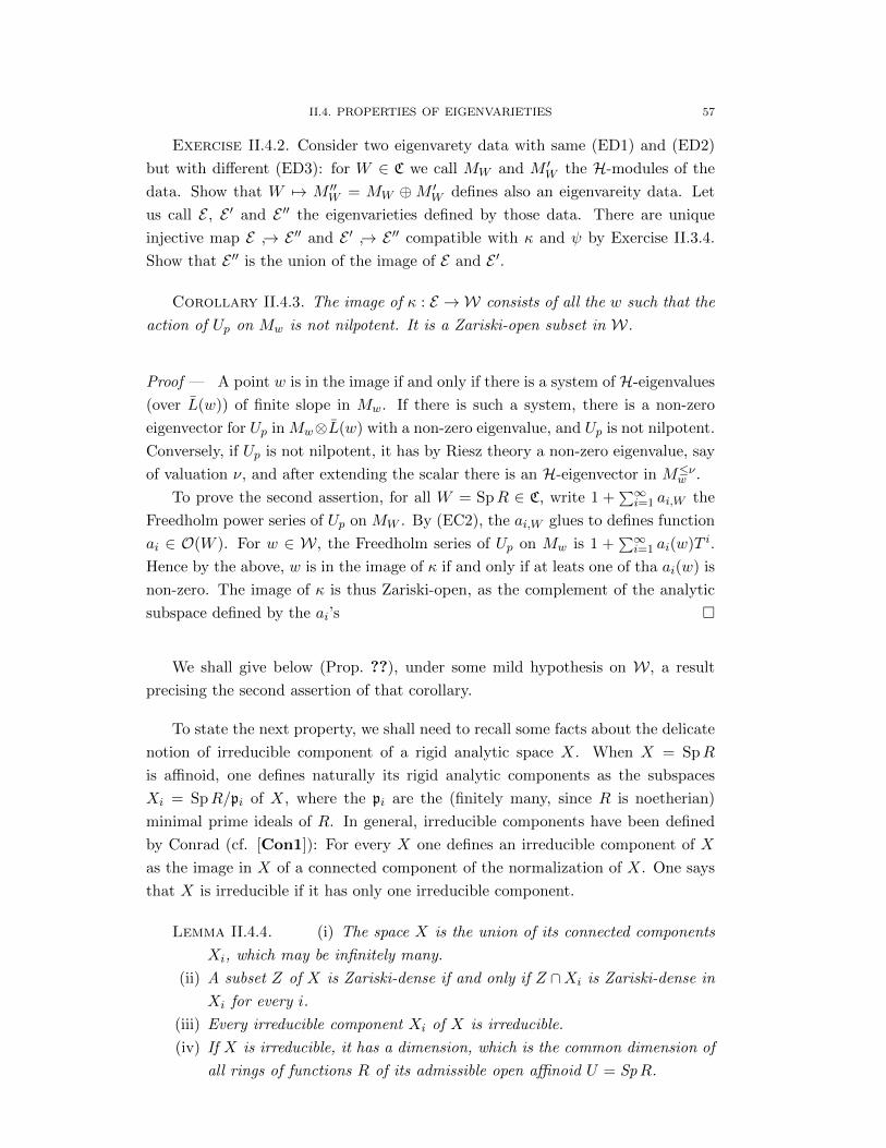
II.4. PROPERTIES OF EIGENVARIETIES 57
Exercise II.4.2. Consider two eigenvarety data with same (ED1) and (ED2)
but with different (ED3): for W ∈ C we call MW and M ′W the H-modules of the
data. Show that W 7→ M ′′W = MW ⊕M ′W defines also an eigenvareity data. Let
us call E , E ′ and E ′′ the eigenvarieties defined by those data. There are unique
injective map E → E ′′ and E ′ → E ′′ compatible with κ and ψ by Exercise II.3.4.
Show that E ′′ is the union of the image of E and E ′.
Corollary II.4.3. The image of κ : E → W consists of all the w such that the
action of Up on Mw is not nilpotent. It is a Zariski-open subset in W.
Proof — A point w is in the image if and only if there is a system of H-eigenvalues
(over L(w)) of finite slope in Mw. If there is such a system, there is a non-zero
eigenvector for Up in Mw⊗L(w) with a non-zero eigenvalue, and Up is not nilpotent.
Conversely, if Up is not nilpotent, it has by Riesz theory a non-zero eigenvalue, say
of valuation ν, and after extending the scalar there is an H-eigenvector in M≤νw .
To prove the second assertion, for all W = SpR ∈ C, write 1 +∑∞i=1 ai,W the
Freedholm power series of Up on MW . By (EC2), the ai,W glues to defines function
ai ∈ O(W ). For w ∈ W, the Freedholm series of Up on Mw is 1 +∑∞i=1 ai(w)T i.
Hence by the above, w is in the image of κ if and only if at leats one of tha ai(w) is
non-zero. The image of κ is thus Zariski-open, as the complement of the analytic
subspace defined by the ai’s
We shall give below (Prop. ??), under some mild hypothesis on W, a result
precising the second assertion of that corollary.
To state the next property, we shall need to recall some facts about the delicate
notion of irreducible component of a rigid analytic space X. When X = SpR
is affinoid, one defines naturally its rigid analytic components as the subspaces
Xi = SpR/pi of X, where the pi are the (finitely many, since R is noetherian)
minimal prime ideals of R. In general, irreducible components have been defined
by Conrad (cf. [Con1]): For every X one defines an irreducible component of X
as the image in X of a connected component of the normalization of X. One says
that X is irreducible if it has only one irreducible component.
Lemma II.4.4. (i) The space X is the union of its connected components
Xi, which may be infinitely many.
(ii) A subset Z of X is Zariski-dense if and only if Z ∩Xi is Zariski-dense in
Xi for every i.
(iii) Every irreducible component Xi of X is irreducible.
(iv) If X is irreducible, it has a dimension, which is the common dimension of
all rings of functions R of its admissible open affinoid U = SpR.

58 II. THE EIGENVARIETY MACHINE
(v) The intersection Xi ∩ U of an irreducible component Xi with an open
admissible affinoid U of X is either empty or a union of irreducible com-
ponents of U .
(vi) If X is irreducible, any non-empty admissible open affinoid U is Zariski-
dense in X.
(vii) If f : X → X ′ is a finite map, the image of an irreducible component of
X by f is an irreducible closed analytic subspace of X ′.
(viii) Let W = SpR is an affinoid, F ∈ RT, F (0) = 1 and Z be the
hypersurface cut out by F in W×A1rig. Then F has a unique decomposition
F =∏i Fi(t)
ni, Fi(0) = 1, where the series Fi(t) generate prime ideals in
RT and the irreducible components of Z are precisely the hypersurface
Zi ⊂W ×A1rig cut out by the Fi.
Proof — For (v), see [Con1, 2.2.9]. For (vii) see [Con1, 2.2.3]. For (viii), see
[Bu, 1.1.10] [Con1, 4.3.2]
One says that a rigid analytic space X is equidimensional of dimension n if
all its connected component have dimension n. By (iv) and (v), this is equivalent
to saying that for all admissible open affinoids U = SpR, R is equi-dimensional
of dimension n in the algebraic sense, that is to say all the domains R/pi for pi
minimal prime ideals have Krull dimension n.
Proposition II.4.5. Assume that W is equidimensional of dimension n. Then
so is E.
Proof — Since being equidimensional of dimension n is a local property as we
just saw, this results from Prop. I.10 and the remark following it.
The next proposition proves the few properties of eigenvarieties for which we
need the full force of Buzzard’s theory, namely the result stated in Remark II.1.14
that the admissible pairs (X, ν) defines an admissible covering of Z.
Proposition II.4.6. (i) The map κ× ψ(Up)−1 : E → W ×A1
rig is finite.
(ii) The eigenvariety E is separated.
(iii) Assume that W is equidimensional, and that a subset of W is Zariski-
open in W is and only if any of its intersection with W (for W ∈ C) is
Zariski-open in W . If D is an irreducible component of E, then κ(D) is
Zariski-open in W
Proof — For (i) it is enough to prove that for all affinoid subdomains W = SpR ⊂W the map κ×ψ(Up)
−1 : EW →W×A1rig is finite. This map factors through a map
EW → ZW , where ZW is the closed subvariety of W×A1rig cut out by the Freedholm
power series FW (T ) of Up acting on MW and it is enough to show that EW → Z

II.5. A COMPARISON THEOREM FOR EIGENVARIETIES 59
is a finite map. Since EW is by definition/construction admissibly covered by the
local pieces EX,ν for adapted pair X ⊂ W, ν ∈ R, and ZW is admissibly covered
by the affinoid ZX,ν for the same pairs (Remark II.1.14), it suffices to show that
the natural maps EX,ν → ZX,ν are finite. But the composition EX,ν → ZX,ν → X
is finite by construction of EX,ν . Assertion (ii) follows from (i) since a finite map is
separated and W ×A1rig is separated.
Let us prove (iii). By the hypothesis made on W, it suffices to show that
κ(D∩EW ) is Zariski-open in W . By Lemma II.4.4, D∩EW is a union of irreducible
component of EW (or is empty, in which case there is nothing to prove), so we may
assume that D ∩ EW is an irreducible component DW of EW . Since EW → ZW is
a finite map, it sends DW to a closed analytic subspace of ZW of same dimension
dim EW = dimW , irreducible by Lemma II.4.4. Since ZW is equidimensional of
dimension dimW = dimW (same proof as Prop. II.4.5), the image of DW in ZW
is an irreducible component Z ′W of ZW , hence is the locus cut out in W ×A1rig by
a power series F ′(T ) = 1 +∑∞i=1 aiT
i ∈ RT. The image by the first projection
map ZW ×W is the complementary in W of the closed analytic subspaces defined
by the equations ai = 0, hence is Zariski-open. But this is also trivially κ(DW ).
Remark II.4.7. The condition in (c) of the above proposition is satisfied for
instance when W is affinoid, or when W is an open ball of radius 1 in A1rig. For
by Lazard’s theory ([L]), a proper subspace is Zariski-closed in W if and only if its
intersection with each of the closed ball of radius r < 1 is finite, that is, Zariski-
closed in that ball.
For the definition of nested, and the easy proof of the next proposition, we refer
the reader to [BC, Definition 7.2.10 and Lemma 7.2.11]:
Proposition II.4.8.
(i) The eigenvariety E is nested.
(ii) If O(E) is provided with the coarsest locally convex topology such that the restric-
tion maps O(E)→ O(U) for every affinoid subdomain U ⊂ E, and if E is reduced,
then the subring O(E)0 of power-bounded functions in O(E) is compact.
A criterion for E to be reduced is given in the next section.
II.5. A comparison theorem for eigenvarieties
In this section we present two very useful theorems of Chenevier: one gives
a sufficient condition for an eigenvariety to be reduced, and the other allows to
compare two eigenvarieties. Both rely on the notion of classical structure.
II.5.1. Classical structures.
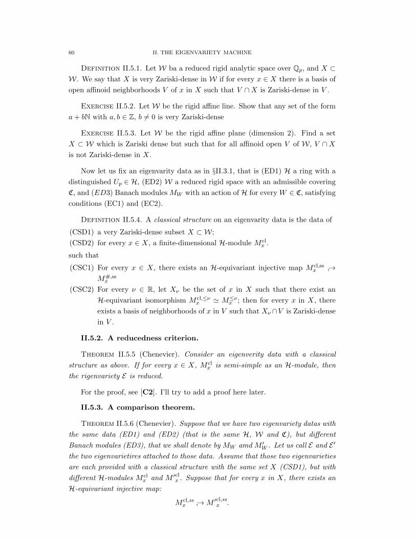
60 II. THE EIGENVARIETY MACHINE
Definition II.5.1. Let W ba a reduced rigid analytic space over Qp, and X ⊂W. We say that X is very Zariski-dense in W if for every x ∈ X there is a basis of
open affinoid neighborhoods V of x in X such that V ∩X is Zariski-dense in V .
Exercise II.5.2. Let W be the rigid affine line. Show that any set of the form
a+ bN with a, b ∈ Z, b 6= 0 is very Zariski-dense
Exercise II.5.3. Let W be the rigid affine plane (dimension 2). Find a set
X ⊂ W which is Zariski dense but such that for all affinoid open V of W, V ∩Xis not Zariski-dense in X.
Now let us fix an eigenvarity data as in §II.3.1, that is (ED1) H a ring with a
distinguished Up ∈ H, (ED2) W a reduced rigid space with an admissible covering
C, and (ED3) Banach modules MW with an action of H for every W ∈ C, satisfying
conditions (EC1) and (EC2).
Definition II.5.4. A classical structure on an eigenvarity data is the data of
(CSD1) a very Zariski-dense subset X ⊂ W;
(CSD2) for every x ∈ X, a finite-dimensional H-module M clx .
such that
(CSC1) For every x ∈ X, there exists an H-equivariant injective map M cl,ssx →
M#,ssx
(CSC2) For every ν ∈ R, let Xν be the set of x in X such that there exist an
H-equivariant isomorphism M cl,≤νx ' M≤νx ; then for every x in X, there
exists a basis of neighborhoods of x in V such that Xν ∩V is Zariski-dense
in V .
II.5.2. A reducedness criterion.
Theorem II.5.5 (Chenevier). Consider an eigenverity data with a classical
structure as above. If for every x ∈ X, M clx is semi-simple as an H-module, then
the rigenvariety E is reduced.
For the proof, see [C2]. I’ll try to add a proof here later.
II.5.3. A comparison theorem.
Theorem II.5.6 (Chenevier). Suppose that we have two eigenvariety datas with
the same data (ED1) and (ED2) (that is the same H, W and C), but different
Banach modules (ED3), that we shall denote by MW amd M ′W . Let us call E and E ′
the two eigenvarietires attached to those data. Assume that those two eigenvarieties
are each provided with a classical structure with the same set X (CSD1), but with
different H-modules M clx and M ′cl
x . Suppose that for every x in X, there exists an
H-equivariant injective map:
M cl,ssx →M ′
cl,ssx .
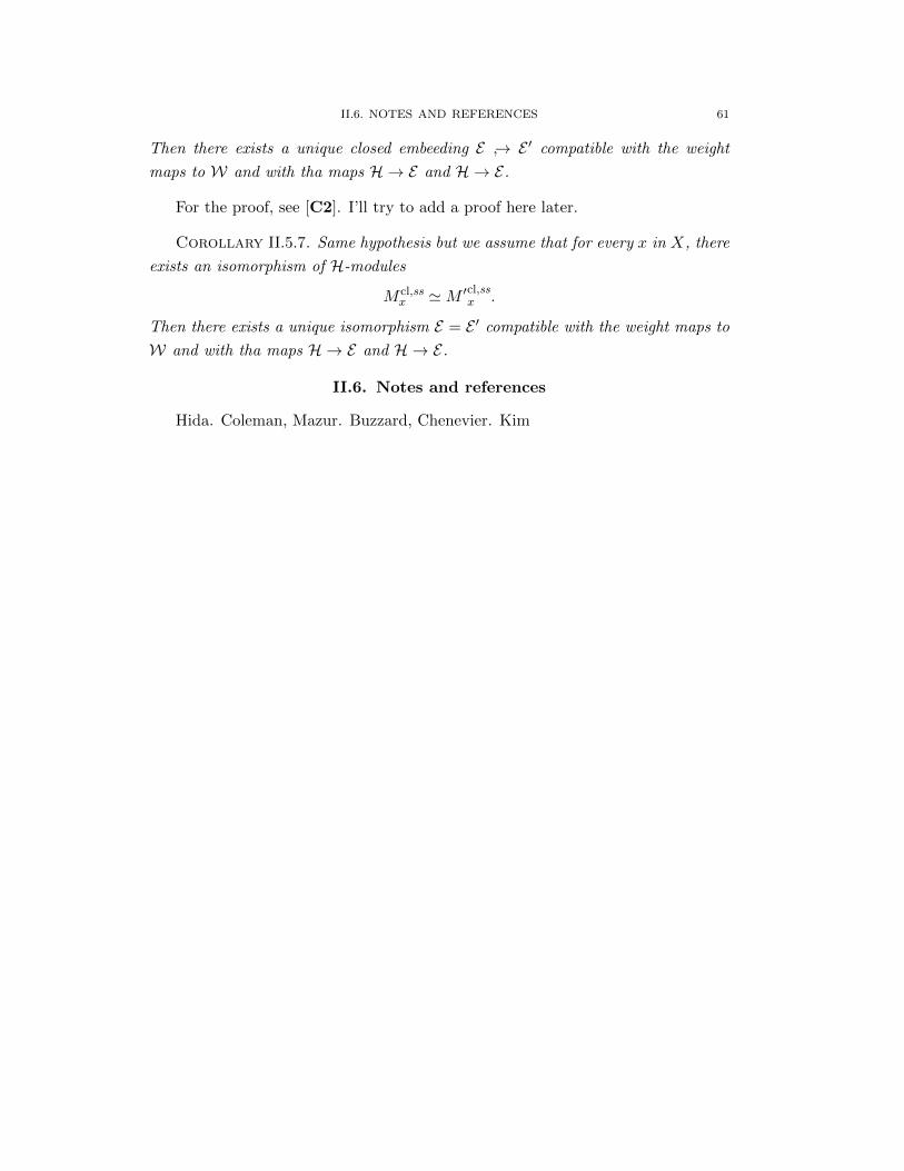
II.6. NOTES AND REFERENCES 61
Then there exists a unique closed embeeding E → E ′ compatible with the weight
maps to W and with tha maps H → E and H → E.
For the proof, see [C2]. I’ll try to add a proof here later.
Corollary II.5.7. Same hypothesis but we assume that for every x in X, there
exists an isomorphism of H-modules
M cl,ssx 'M ′cl,ss
x .
Then there exists a unique isomorphism E = E ′ compatible with the weight maps to
W and with tha maps H → E and H → E.
II.6. Notes and references
Hida. Coleman, Mazur. Buzzard, Chenevier. Kim


Part 2
Modular Symbols, the Eigencurve,and p-adic L-functions


CHAPTER III
Modular symbols
III.1. Abstract modular symbols
III.1.1. Notion of modular symbols. Let ∆ be the abelian group of divisors
on P1(Q), that is the group of formal sums∑x∈P1(Q) nxx, with nx ∈ Z and nx = 0
for all x but a finite number. Let ∆0 be the subgroup of divisors of degree 0, that
is such that∑x nx = 0. The natural action of GL2(Q) on P1(Q), γ · x = ax+b
cx+d if
γ =
Ça bc d
å, induces an action of GL2(Q) on ∆ and on ∆0, respecting the group
structures.
Exercise III.1.1. 1.– Prove Manin’s lemma: ∆0 is generated, as an SL2(Z)-
module, by the divisor ∞ − 0. You can proceed as follows:
a.– Prove Pick’s lemma: a non-flat triangle with vertices in Z2 has area ≥ 1/2,
with equality if and only if the three vertices are the only points of Z2 in the
triangle.
b.– Let a/c and b/d be two irreducible fractions. Show that there exists γ ∈SL2(Z) such that γ(∞−0) = a/c−b/d if and only if the triangle of vertices
(0, 0), (a, c), (b, d) has area 1/2.
c.– Conclude.
2.– If Γ is a finite index subgroup of GL2(Z), then ∆0 is finitely generated as a
Z[Γ]-module.
3.– Prove Pick’s theorem: If P is a polygon whose all vertices are in Z2, then
the area of P is I + F2 − 1 where I is the number of points of Z2 in the interior of
P , and F the number of points of Z2 on its boundary.
Let Γ be a congruence subgroup of SL2(Z). For V any right Γ-module, that
is any abelian group with a Γ-action on the right (denoted bt v 7→ v|γ), there is a
right action of Γ on Hom(∆0, V ) given by
(φ|γ)(D) = φ(γ ·D)|γ(14)
for γ in Γ and we define the group of V -valued modular symbols (for Γ),
SymbΓ(V ) = Hom(∆0, V )Γ.
Observe that if V is an R-module, for R any commutative ring, with a right Γ-action
that preserves its R-module structure, then SymbΓ(V ) has an obvious structure of
R-module. The construction V 7→ SymbΓ(V ) is functorial (from the categories of
R-modules with right Γ-actions to the category of R-modules).
65
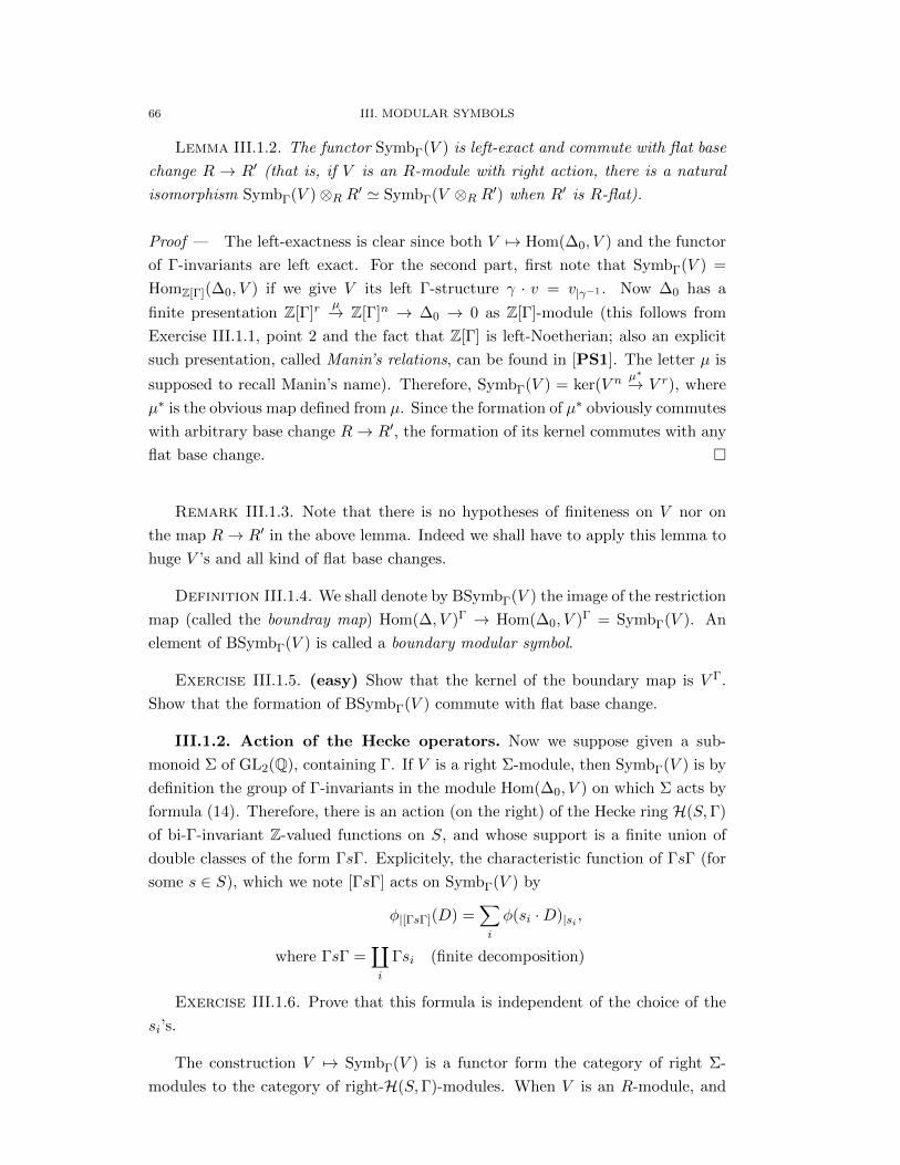
66 III. MODULAR SYMBOLS
Lemma III.1.2. The functor SymbΓ(V ) is left-exact and commute with flat base
change R → R′ (that is, if V is an R-module with right action, there is a natural
isomorphism SymbΓ(V )⊗R R′ ' SymbΓ(V ⊗R R′) when R′ is R-flat).
Proof — The left-exactness is clear since both V 7→ Hom(∆0, V ) and the functor
of Γ-invariants are left exact. For the second part, first note that SymbΓ(V ) =
HomZ[Γ](∆0, V ) if we give V its left Γ-structure γ · v = v|γ−1 . Now ∆0 has a
finite presentation Z[Γ]rµ→ Z[Γ]n → ∆0 → 0 as Z[Γ]-module (this follows from
Exercise III.1.1, point 2 and the fact that Z[Γ] is left-Noetherian; also an explicit
such presentation, called Manin’s relations, can be found in [PS1]. The letter µ is
supposed to recall Manin’s name). Therefore, SymbΓ(V ) = ker(V n µ∗→ V r), where
µ∗ is the obvious map defined from µ. Since the formation of µ∗ obviously commutes
with arbitrary base change R→ R′, the formation of its kernel commutes with any
flat base change.
Remark III.1.3. Note that there is no hypotheses of finiteness on V nor on
the map R→ R′ in the above lemma. Indeed we shall have to apply this lemma to
huge V ’s and all kind of flat base changes.
Definition III.1.4. We shall denote by BSymbΓ(V ) the image of the restriction
map (called the boundray map) Hom(∆, V )Γ → Hom(∆0, V )Γ = SymbΓ(V ). An
element of BSymbΓ(V ) is called a boundary modular symbol.
Exercise III.1.5. (easy) Show that the kernel of the boundary map is V Γ.
Show that the formation of BSymbΓ(V ) commute with flat base change.
III.1.2. Action of the Hecke operators. Now we suppose given a sub-
monoid Σ of GL2(Q), containing Γ. If V is a right Σ-module, then SymbΓ(V ) is by
definition the group of Γ-invariants in the module Hom(∆0, V ) on which Σ acts by
formula (14). Therefore, there is an action (on the right) of the Hecke ring H(S,Γ)
of bi-Γ-invariant Z-valued functions on S, and whose support is a finite union of
double classes of the form ΓsΓ. Explicitely, the characteristic function of ΓsΓ (for
some s ∈ S), which we note [ΓsΓ] acts on SymbΓ(V ) by
φ|[ΓsΓ](D) =∑i
φ(si ·D)|si ,
where ΓsΓ =∐i
Γsi (finite decomposition)
Exercise III.1.6. Prove that this formula is independent of the choice of the
si’s.
The construction V 7→ SymbΓ(V ) is a functor form the category of right Σ-
modules to the category of right-H(S,Γ)-modules. When V is an R-module, and

III.1. ABSTRACT MODULAR SYMBOLS 67
the action of Σ is by R-linear operators, then obviously the Hecke operators are
R-linear on SymbΓ(V ).
We use the classical notation Tl for [Γ
Ç1 00 l
åΓ], replaced by Ul when l divides
the level of Γ (that is l|N when Γ = Γ1(N) or Γ0(N)).
Exercise III.1.7. (easy) Let Γ = Γ1(N) or Γ0(N). If V is Q-vector space,
with a right action of Σ, and n ∈ Z, we left V (n) be the group V with action of
s ∈ Σ multiplied by (det s)n. That is, if v ∈ V , v|V (n)s = (det s)nv|s. Note that the
Γ-action on V and V (n) are the same, so SymbΓ(V ) = SymbΓ(V (n)). However,
the action of the Hecke operators are different. Show that the action of Tl for l 6 |N(resp. Ul for l|N) on SymbΓ(V (n)) is ln (resp. pn) times its action on SymbΓ(V ).
III.1.3. Relations with cohomology. Let H be an abelian group. If X is
a topological space, the constant sheaf HX attached to H is defined as the sheaf in
abelian groups attached to the presheaf U 7→ H for any open U ⊂ X.
A local system (or locally constant sheaf) on a space X is a sheaf in abelian
groups G on X such that there exists a group H such that for any x ∈ X, there is
an open set U of X containing x such that G|U ' HU as sheaves of abelian group
over U .
The abelian group H, if it exists, is obviously unique, up to isomorphism. The
fiber of a local system at any point x is isomorphic to H.
Exercise III.1.8. Assume that X is path-connected. Let G be a locally free
sheaf on X.
1.– If γ is a path in X from x to y, explain how to define an isomorphism
iγ : Gx → Gy, and show that it iγ depends only of the homotopy class in γ.
2.– If γ′ is a path from y to z, show that iγ′ iγ = iγγ′ where γ γ′ is the
concatenation of γ and γ′. In particular, if x ∈ X, we have a natural action of
π1(X,x) on Gx called the monodromy action.
3.– Show that if x ∈ X is fixed, you have defined a functor G 7→ Gx from the
category of locally constant sheaves to the category of abelian groups with an action
of π1(X,x). Explain how this functor depends on the choice of the base point x.
If we assume some relatively mild hypothesis on X, such as its being locally
connected, and locally simply connected, then this functor is an equivalence of
category. (The inverse functor is essentially the construction V 7→ V explained
below, with Γ replaced by π1(X,x) and U(Γ) replaced by the universal cover of
X.)
Let us recall that Steenrod ([ST]) defined (on some mild assumptions on X
that will always be satisfied in our situations) groups of cohomology with value
in a local systems H i(X,G), homology Hi(X,G), and cohomology with compact
support H ic(X,G)
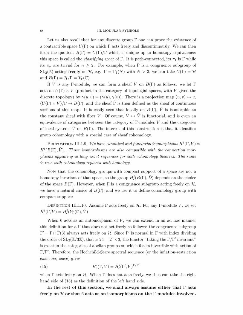
68 III. MODULAR SYMBOLS
Let us also recall that for any discrete group Γ one can prove the existence of
a contractible space U(Γ) on which Γ acts freely and discontinuously. We can then
form the quotient B(Γ) = U(Γ)/Γ which is unique up to homotopy equivalence:
this space is called the classifying space of Γ. It is path-connected, its π1 is Γ while
its πn are trivial for n ≥ 2. For example, when Γ is a congruence subgroup of
SL2(Z) acting freely on H, e.g. Γ = Γ1(N) with N > 3, we can take U(Γ) = Hand B(Γ) = H/Γ = YΓ(C).
If V is any Γ-module, we can form a sheaf V on B(Γ) as follows: we let Γ
acts on U(Γ) × V (product in the category of topologial spaces, with V given the
discrete topology) by γ(u, v) = (γ(u), γ(v)). There is a projection map (u, v) 7→ u,
(U(Γ) × V )/Γ → B(Γ), and the sheaf Γ is then defined as the sheaf of continuous
sections of this map. It is easily seen that locally on B(Γ), V is isomorphic to
the constant sheaf with fiber V . Of course, V 7→ V is functorial, and is even an
equivalence of categories between the category of Γ-modules V and the categories
of local systems V on B(Γ). The interest of this construction is that it identifies
group cohomology with a special case of sheaf cohomology.
Proposition III.1.9. We have canonical and functorial isomorphisms H i(Γ, V ) 'H i(B(Γ), V ). Those isomorphisms are also compatible with the connection mor-
phisms appearing in long exact sequences for both cohomology theories. The same
is true with cohomology replaced with homology.
Note that the cohomology groups with compact support of a space are not a
homotopy invariant of that space, so the group H ic(B(Γ), D) depends on the choice
of the space B(Γ). However, when Γ is a congruence subgroup acting freely on H,
we have a natural choice of B(Γ), and we use it to define cohomology group with
compact support:
Definition III.1.10. Assume Γ acts freely on H. For any Γ-module V , we set
H ic(Γ, V ) = H i
c(YΓ(C), V )
When 6 acts as an automorphism of V , we can extend in an ad hoc manner
this definition for a Γ that does not act freely as follows: the congruence subgroup
Γ′ = Γ ∩ Γ(3) always acts freely on H. Since Γ′ is normal in Γ with index dividing
the order of SL2(Z/3Z), that is 24 = 23×3, the functor ”taking the Γ/Γ′ invariant”
is exact in the categories of abelian groups on which 6 acts invertible with action of
Γ/Γ′. Therefore, the Hochchild-Serre spectral sequence (or the inflation-restriction
exact sequence) gives
H ic(Γ, V ) = H i
c(Γ′, V )Γ/Γ′(15)
when Γ acts freely on H. When Γ does not acts freely, we thus can take the right
hand side of (15) as the definition of the left hand side.
In the rest of this section, we shall always assume either that Γ acts
freely on H or that 6 acts as an isomorphisms on the Γ-modules involved.
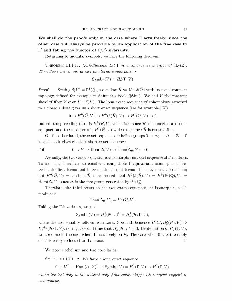
III.1. ABSTRACT MODULAR SYMBOLS 69
We shall do the proofs only in the case where Γ acts freely, since the
other case will always be provable by an application of the free case to
Γ′ and taking the functor of Γ/Γ′-invariants.
Returning to modular symbols, we have the following theorem.
Theorem III.1.11. (Ash-Stevens) Let Γ be a congruence ungroup of SL2(Z).
Then there are canonical and functorial isomorphisms
SymbΓ(V ) ' H1c (Γ, V )
Proof — Setting δ(H) = P1(Q), we endow H := H∪ δ(H) with its usual compact
topology defined for example in Shimura’s book ([Shi]). We call V the constant
sheaf of fiber V over H ∪ δ(H). The long exact sequence of cohomology attached
to a closed subset gives us a short exact sequence (see for example [G])
0→ H0(H, V )→ H0(δ(H), V )→ H1c (H, V )→ 0
Indeed, the preceding term is H0c (H, V ) which is 0 since H is connected and non-
compact, and the next term is H1(H, V ) which is 0 since H is contractible.
On the other hand, the exact sequence of abelian groups 0→ ∆0 → ∆→ Z→ 0
is split, so it gives rise to a short exact sequence
0→ V → Hom(∆, V )→ Hom(∆0, V )→ 0.(16)
Actually, the two exact sequences are isomorphic as exact sequence of Γ-modules.
To see this, it suffices to construct compatible Γ-equivariant isomorphisms be-
tween the first terms and between the second terms of the two exact sequences;
but H0(H, V ) = V since H is connected, and H0(δ(H), V ) = H0(P1(Q), V ) =
Hom(∆, V ) since ∆ is the free group generated by P1(Q).
Therefore, the third terms on the two exact sequences are isomorphic (as Γ-
modules):
Hom(∆0, V ) = H1c (H, V ).
Taking the Γ-invariants, we get
SymbΓ(V ) = H1c (H, V )Γ = H1
c (H/Γ, V ),
where the last equality follows from Leray Spectral Sequence H i(Γ, Hjc (H), V ) ⇒
H i+jc (H/Γ, V ), noting a second time that H0
c (H, V ) = 0. By definition of H1c (Γ, V ),
we are done in the case where Γ acts freely on H. The case when 6 acts invertibly
on V is easily reducted to that case.
We note a scholium and two corollaries.
Scholium III.1.12. We have a long exact sequence
0→ V Γ → Hom(∆, V )Γ → SymbΓ(V ) = H1c (Γ, V )→ H1(Γ, V ),
where the last map is the natural map from cohomology with compact support to
cohomology.
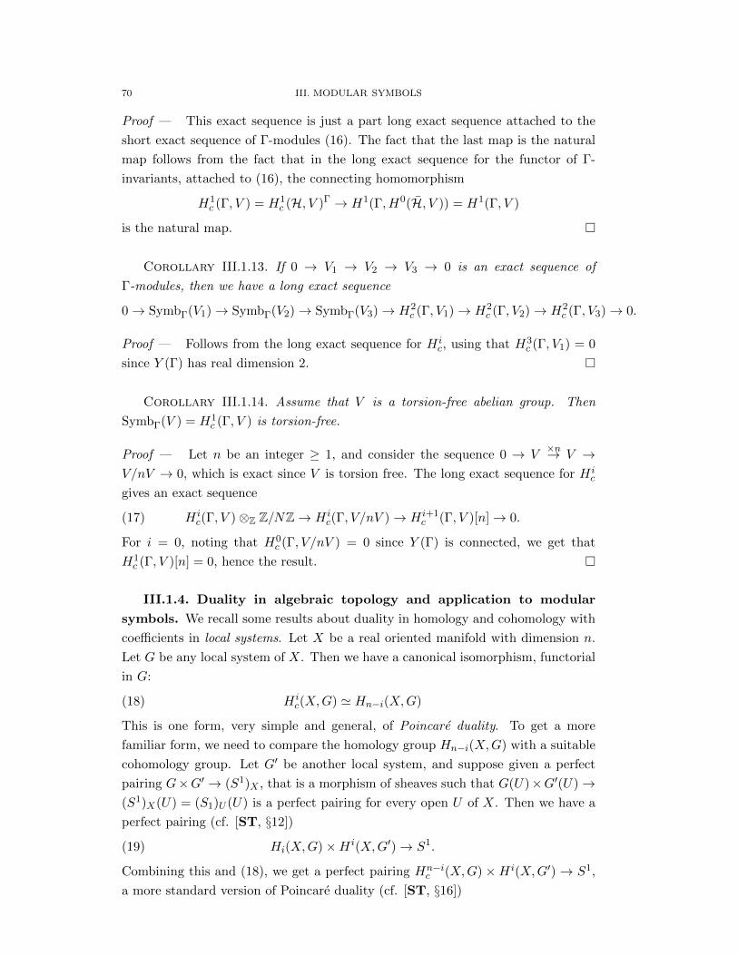
70 III. MODULAR SYMBOLS
Proof — This exact sequence is just a part long exact sequence attached to the
short exact sequence of Γ-modules (16). The fact that the last map is the natural
map follows from the fact that in the long exact sequence for the functor of Γ-
invariants, attached to (16), the connecting homomorphism
H1c (Γ, V ) = H1
c (H, V )Γ → H1(Γ, H0(H, V )) = H1(Γ, V )
is the natural map.
Corollary III.1.13. If 0 → V1 → V2 → V3 → 0 is an exact sequence of
Γ-modules, then we have a long exact sequence
0→ SymbΓ(V1)→ SymbΓ(V2)→ SymbΓ(V3)→ H2c (Γ, V1)→ H2
c (Γ, V2)→ H2c (Γ, V3)→ 0.
Proof — Follows from the long exact sequence for H ic, using that H3
c (Γ, V1) = 0
since Y (Γ) has real dimension 2.
Corollary III.1.14. Assume that V is a torsion-free abelian group. Then
SymbΓ(V ) = H1c (Γ, V ) is torsion-free.
Proof — Let n be an integer ≥ 1, and consider the sequence 0 → V×n→ V →
V/nV → 0, which is exact since V is torsion free. The long exact sequence for H ic
gives an exact sequence
H ic(Γ, V )⊗Z Z/NZ→ H i
c(Γ, V/nV )→ H i+1c (Γ, V )[n]→ 0.(17)
For i = 0, noting that H0c (Γ, V/nV ) = 0 since Y (Γ) is connected, we get that
H1c (Γ, V )[n] = 0, hence the result.
III.1.4. Duality in algebraic topology and application to modular
symbols. We recall some results about duality in homology and cohomology with
coefficients in local systems. Let X be a real oriented manifold with dimension n.
Let G be any local system of X. Then we have a canonical isomorphism, functorial
in G:
H ic(X,G) ' Hn−i(X,G)(18)
This is one form, very simple and general, of Poincare duality. To get a more
familiar form, we need to compare the homology group Hn−i(X,G) with a suitable
cohomology group. Let G′ be another local system, and suppose given a perfect
pairing G×G′ → (S1)X , that is a morphism of sheaves such that G(U)×G′(U)→(S1)X(U) = (S1)U (U) is a perfect pairing for every open U of X. Then we have a
perfect pairing (cf. [ST, §12])
Hi(X,G)×H i(X,G′)→ S1.(19)
Combining this and (18), we get a perfect pairing Hn−ic (X,G) ×H i(X,G′) → S1,
a more standard version of Poincare duality (cf. [ST, §16])

III.1. ABSTRACT MODULAR SYMBOLS 71
Another scenario is when G is a locally constant sheaf of R-modules, where R
is a commutative ring. Set G∨ = HomX(G,RX), where HomX means morphism of
sheaves in R-modules, and assume that the pairing G×G∨ → R is perfect. Then
there is a natural R-linear pairing
H i(X,G)×Hi(X,G∨)→ R(20)
but it is not necessarily perfect.
Exercise III.1.15. Give an example, with R = Z, G = G′ = ZX , where the
above a pairing is not perfect.
However, the pairing (20) is perfect when R is a field of characteristic 0 (refer-
ence?). Another situation where this pairing is perfect is when R = Z/lnZ and G
is finite over R, because in this case G′ = G∨.
In the above situation, let us rewrite the second pairing using (18): we obtain
a (not always perfect)
H i(X,G∨)×Hn−ic (X,G)→ R.(21)
But we also have a pairing given by the cup-product
H ic(X,G
∨)×Hn−ic (X,G)→ Hn
c (X,R) ' R,(22)
This pairing is compatible with the pairing (21), that is there is a diagram
H i(X,G∨)×Hn−ic (X,G) // R
H ic(X,G
∨)×Hn−ic (X,G)
β×Id
OO
// R
=
OO(23)
where β denotes the natural map
β : H ic(X,−)→ H i(X,−)(24)
The interior cohomology H i! (X,G) is defined as the image of β : H i
c(X,G) →H i(X,G) (in the context of modular symbols, where X is a modular curve, it is
also called parabolic cohomology and denoted H ip) The preceding paragraph implies
formally that if x ∈ H i! (X,G
∨), y ∈ Hn−i(X,G) and x = β(x0), y = β(y0) then
the image of (x0, y0) by the pairing (22) does not depend on x0 and y0, but only
on x and y.
Exercise III.1.16. (easy) Prove it.
Therefore we get a pairing
H i! (X,G
∨)×Hn−i! (X,G)→ R.(25)
Exercise III.1.17. (easy) Deduce from what we have said above that this
pairing is perfect when R is a field of characteristic 0, or when R = Z/lnZ and G
is finite.
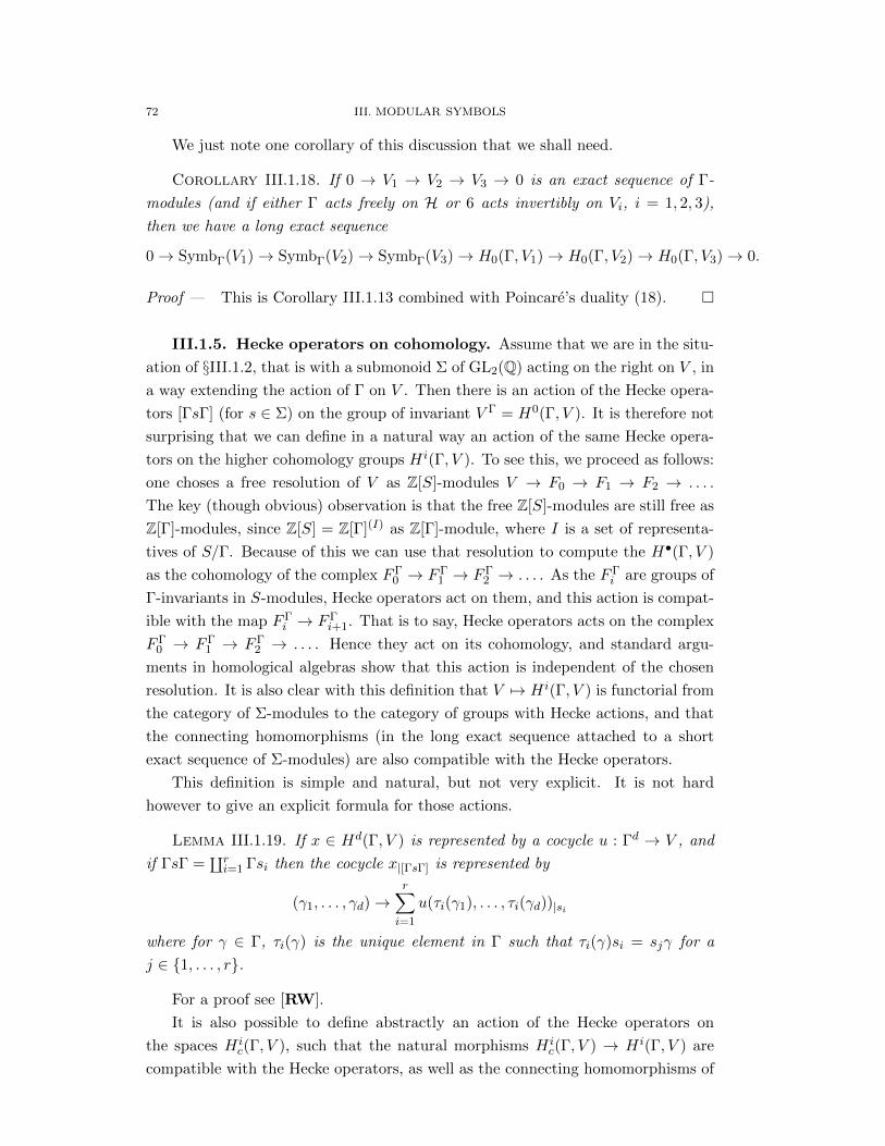
72 III. MODULAR SYMBOLS
We just note one corollary of this discussion that we shall need.
Corollary III.1.18. If 0 → V1 → V2 → V3 → 0 is an exact sequence of Γ-
modules (and if either Γ acts freely on H or 6 acts invertibly on Vi, i = 1, 2, 3),
then we have a long exact sequence
0→ SymbΓ(V1)→ SymbΓ(V2)→ SymbΓ(V3)→ H0(Γ, V1)→ H0(Γ, V2)→ H0(Γ, V3)→ 0.
Proof — This is Corollary III.1.13 combined with Poincare’s duality (18).
III.1.5. Hecke operators on cohomology. Assume that we are in the situ-
ation of §III.1.2, that is with a submonoid Σ of GL2(Q) acting on the right on V , in
a way extending the action of Γ on V . Then there is an action of the Hecke opera-
tors [ΓsΓ] (for s ∈ Σ) on the group of invariant V Γ = H0(Γ, V ). It is therefore not
surprising that we can define in a natural way an action of the same Hecke opera-
tors on the higher cohomology groups H i(Γ, V ). To see this, we proceed as follows:
one choses a free resolution of V as Z[S]-modules V → F0 → F1 → F2 → . . . .
The key (though obvious) observation is that the free Z[S]-modules are still free as
Z[Γ]-modules, since Z[S] = Z[Γ](I) as Z[Γ]-module, where I is a set of representa-
tives of S/Γ. Because of this we can use that resolution to compute the H•(Γ, V )
as the cohomology of the complex FΓ0 → FΓ
1 → FΓ2 → . . . . As the FΓ
i are groups of
Γ-invariants in S-modules, Hecke operators act on them, and this action is compat-
ible with the map FΓi → FΓ
i+1. That is to say, Hecke operators acts on the complex
FΓ0 → FΓ
1 → FΓ2 → . . . . Hence they act on its cohomology, and standard argu-
ments in homological algebras show that this action is independent of the chosen
resolution. It is also clear with this definition that V 7→ H i(Γ, V ) is functorial from
the category of Σ-modules to the category of groups with Hecke actions, and that
the connecting homomorphisms (in the long exact sequence attached to a short
exact sequence of Σ-modules) are also compatible with the Hecke operators.
This definition is simple and natural, but not very explicit. It is not hard
however to give an explicit formula for those actions.
Lemma III.1.19. If x ∈ Hd(Γ, V ) is represented by a cocycle u : Γd → V , and
if ΓsΓ =∐ri=1 Γsi then the cocycle x|[ΓsΓ] is represented by
(γ1, . . . , γd)→r∑i=1
u(τi(γ1), . . . , τi(γd))|si
where for γ ∈ Γ, τi(γ) is the unique element in Γ such that τi(γ)si = sjγ for a
j ∈ 1, . . . , r.
For a proof see [RW].
It is also possible to define abstractly an action of the Hecke operators on
the spaces H ic(Γ, V ), such that the natural morphisms H i
c(Γ, V ) → H i(Γ, V ) are
compatible with the Hecke operators, as well as the connecting homomorphisms of

III.2. CLASSICAL MODULAR SYMBOLS AND THEIR RELATIONS TO MODULAR FORMS 73
the long exact sequence of cohomology with compact support. The details can be
found in [H5]. We shall mainly need the action of the Hecke operators on H1c (Γ, V )
and in this case we can simply say that we define the action of Hecke operators [ΓsΓ]
by transfer of structure using our canonical isomorphism H1c (Γ, V ) = SymbΓ(V ).
The fact that, with this definition, the natural map H1c (Γ, V )→ H1(Γ, V ) is Hecke-
compatible follows from the fact that this map is a connecting homorphism in a long
exact sequence attached to a short exact sequence of Σ-modules by Scholium III.1.12
and its proof.
It is possible to give a simple geometric description of the action of the Hecke
operators [ΓsΓ] on H i(Γ, V ) or H ic(Γ, V ), when s ∈ Σ and det s > 0. We assume
for simplicity that Γ acts freely on H. Set Φ = Γ ∩ sΓs−1 which is of finite index
in Γ, and in sΓs−1. We write YΓ, YΦ, etc. for H/Γ, etc. On those manifolds we
have the sheafs VΓ, VΦ, etc. Using the action of s on H (since det s > 0) and
on V , we can easily define an isomorphism [s] : Ys−1Φs → YΦ which identifies the
sheaves VΦ with Vs−1Φs, hence a map [s]∗ : H i(YΦ, VΦ) → H i(Ys−1Φs, Vs−1Φs). On
the other hand, we have finite maps pr1 : YΦ → YΓ and pr2 : Ys−1Φs → YΓ given
by the inclusions Γ ⊂ Φ and Γ ⊂ s−1Φs, and compatible with the various sheaves
V . Hence we get a pull-back map pr∗1 : H i(YΓ, VΓ) → H i(YΦ, Vφ), and since pr2
is finite, a push-forward (or trace) map (pr2)∗ : H i(Ys−1Φs, Vs−1Φs) → H i(YΓ, VΓ).
The composition
(pr2)∗ [s]∗ pr∗1
is an endomorphism of H i(YΓ, VΓ) = H i(Γ, V ). It is easy to see that this isomor-
phism is the Hecke operator [ΓsΓ] defined above.
III.2. Classical modular symbols and their relations to modular forms
Concerning spaces of modular forms and Hecke operators acting on them, we
use the same notations and conventions recalled in §I.6.4
III.2.1. The monoid S. We consider the following monoid
S = GL2(Q) ∩M2(Z).
We note that this monoid is provided with an anti-involution
γ 7→ γ′ = det(γ)γ−1.
The anti in anti-involution means (γ1γ2)′ = γ′2γ′1. Explicitly, γ′ =
Çd −b−c a
åif
γ =
Ça bc d
å.
This anti-involution allows us to see any left-S-module as a right-S-module,
and conversely : if S acts on V of the left, we define an action on the right by
letting γ acts on the right on V through the left-action of γ′ on V , and conversely:
for v ∈ V, γ ∈ Sγ · v = v|γ′ .
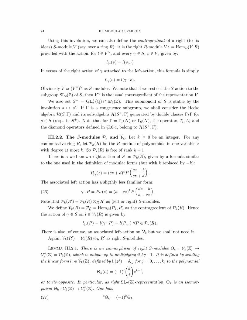
74 III. MODULAR SYMBOLS
Using this involution, we can also define the contragredient of a right (to fix
ideas) S-module V (say, over a ring R): it is the right R-module V ∨ = HomR(V,R)
provided with the action, for l ∈ V ∨, and every γ ∈ S, v ∈ V , given by:
l|γ(v) = l(v|γ′)
In terms of the right action of γ attached to the left-action, this formula is simply
l|γ(v) = l(γ · v).
Obviously V ' (V ∨)∨ as S-modules. We note that if we restrict the S-action to the
subgroup SL2(Z) of S, then V ∨ is the usual contragredient of the representation V .
We also set S+ = GL+2 (Q) ∩ M2(Z). This submonoid of S is stable by the
involution s 7→ s′. If Γ is a congruence subgroup, we shall consider the Hecke
algebra H(S,Γ) and its sub-algebra H(S+,Γ) generated by double classes ΓsΓ for
s ∈ S (resp. in S+). Note that for Γ = Γ1(N) or Γ0(N), the operators Tl, Ul and
the diamond operators defined in §I.6.4, belong to H(S+,Γ).
III.2.2. The S-modules Pk and Vk. Let k ≥ 0 be an integer. For any
commutative ring R, let Pk(R) be the R-module of polynomials in one variable z
with degree at most k. So Pk(R) is free of rank k + 1
There is a well-known right-action of S on Pk(R), given by a formula similar
to the one used in the definition of modular forms (but with k replaced by −k):
P|γ(z) = (cz + d)kP
Åaz + b
cz + d
ã.
The associated left action has a sligthly less familiar form:
γ · P = Pγ′(z) = (a− cz)kPÅdz − ba− cz
ã.(26)
Note that Pk(R′) = Pk(R)⊗R R′ as (left or right) S-modules.
We define Vk(R) = P∨k = HomR(Pk, R) as the contragredient of Pk(R). Hence
the action of γ ∈ S on l ∈ Vk(R) is given by
l|γ(P ) = l(γ · P ) = l(P|γ′) ∀P ∈ Pk(R).
There is also, of course, an associated left-action on Vk but we shall not need it.
Again, Vk(R′) = Vk(R)⊗R R′ as right S-modules.
Lemma III.2.1. There is an isomorphism of right S-modules Θk : Vk(Z) →V∨k (Z) = Pk(Z), which is unique up to multiplying it by −1. It is defined by sending
the linear form li ∈ Vk(Z), defined by li(zj) = δi,j for j = 0, . . . , k, to the polynomial
Θk(li) = (−1)iÇk
i
åzk−i,
or to its opposite. In particular, as right SL2(Z)-representation, Θk is an isomor-
phism Θk : Vk(Z)→ V∨k (Z). One has:
tΘk = (−1)kΘk(27)
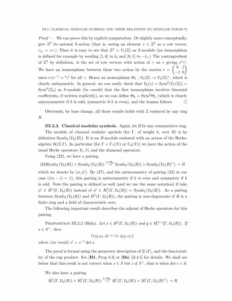
III.2. CLASSICAL MODULAR SYMBOLS AND THEIR RELATIONS TO MODULAR FORMS 75
Proof — We can prove this by explicit computation. Or slightly more conceptually,
give Z2 its natural S-action (that is, seeing an element v ∈ Z2 as a row vector,
v|γ = vγ.) Then it is easy to see that Z2 ' V1(Z) as S-module (an isomorphism
is defined for example by sending [1, 0] to l0 and [0, 1] to −l1.) The contragredient
of Z2 by definition, is the set of row vectors with action of γ on v giving vtγ′.
We have an isomorphism between those two action by the matrix e =
Ç0 1−1 0
åsince eγe−1 = tγ′ for all γ. Hence an isomorphism Θ1 : V1(Z) → V1(Z)∨, which is
clearly antisymetric. In general, we can easily check that Vk(z) = Symk(V1(Z)) =
Symk(Z2) as S-module (be careful that the first isomorphism involves binomial
coefficients, if written explicitly), so we can define Θk = SymkΘ1 (which is clearly
antysymmetric if k is odd, symmetric if k is even), and the lemma follows
Obviously, by base change, all those results holds with Z replaced by any ring
R.
III.2.3. Classical modular symbols. Again, let R be any commutative ring.
The module of classical modular symbols (for Γ, of weight k, over R) is by
definition SymbΓ(Vk(R)). It is an R-module endowed with an action of the Hecke-
algebra H(S,Γ). In particular (for Γ = Γ1(N) or Γ0(N)) we have the action of the
usual Hecke operators Tl, Ul and the diamond operators.
Using (22), we have a pairing
SymbΓ(Vk(R))× SymbΓ(Vk(R))1×Θk→ SymbΓ(Vk(R))× SymbΓ(Vk(R)∨)→ R(28)
which we denote by (φ, φ′). By (27), and the antisymmetry of pairing (22) in our
case (i(n − i) = 1), this pairing is antisymmetric if k is even and symmetric if k
is odd. Note the pairing is defined as well (and we use the same notation) if take
φ′ ∈ H1(Γ,Vk(R)) instead of φ′ ∈ H1c (Γ,Vk(R)) = SymbΓ(Vk(R)). As a pairing
between SymbΓ(Vk(R)) and H1(Γ,Vk(R)), the pairing is non-degenerate if R is a
finite ring and a field of characteristic zero.
The following important result describes the adjoint of Hecke operators for this
pairing.
Proposition III.2.2 (Hida). Let x ∈ H i(Γ,Vk(R)) and y ∈ H2−ic (Γ,Vk(R)). If
s ∈ S+, then
(x|[ΓsΓ], y) = (x, y|[Γs′Γ]),
where (we recall) s′ = s−1 det s.
The proof is formal using the geometric description of [ΓsΓ], and the functorial-
ity of the cup product. See [H1, Prop 3.3] or [Shi, §3.4.5] for details. We shall see
below that this result is not correct when s ∈ S but s 6∈ S+, that is when det s < 0.
We also have a pairing
H1! (Γ,Vk(R))×H1
! (Γ,Vk(R))1×Θk→ H1
! (Γ,Vk(R))×H1! (Γ,Vk(R)∨)→ R
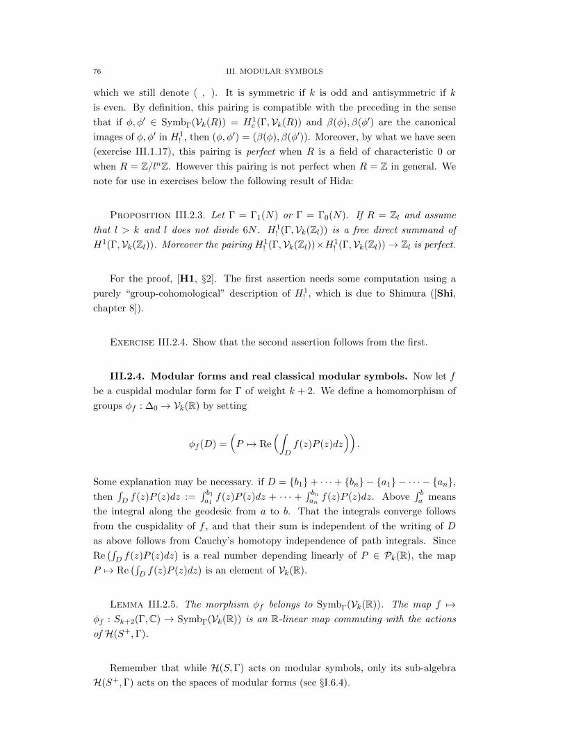
76 III. MODULAR SYMBOLS
which we still denote ( , ). It is symmetric if k is odd and antisymmetric if k
is even. By definition, this pairing is compatible with the preceding in the sense
that if φ, φ′ ∈ SymbΓ(Vk(R)) = H1c (Γ,Vk(R)) and β(φ), β(φ′) are the canonical
images of φ, φ′ in H1! , then (φ, φ′) = (β(φ), β(φ′)). Moreover, by what we have seen
(exercise III.1.17), this pairing is perfect when R is a field of characteristic 0 or
when R = Z/lnZ. However this pairing is not perfect when R = Z in general. We
note for use in exercises below the following result of Hida:
Proposition III.2.3. Let Γ = Γ1(N) or Γ = Γ0(N). If R = Zl and assume
that l > k and l does not divide 6N . H1! (Γ,Vk(Zl)) is a free direct summand of
H1(Γ,Vk(Zl)). Moreover the pairing H1! (Γ,Vk(Zl))×H1
! (Γ,Vk(Zl))→ Zl is perfect.
For the proof, [H1, §2]. The first assertion needs some computation using a
purely “group-cohomological” description of H1! , which is due to Shimura ([Shi,
chapter 8]).
Exercise III.2.4. Show that the second assertion follows from the first.
III.2.4. Modular forms and real classical modular symbols. Now let f
be a cuspidal modular form for Γ of weight k + 2. We define a homomorphism of
groups φf : ∆0 → Vk(R) by setting
φf (D) =
ÅP 7→ Re
Å∫Df(z)P (z)dz
ãã.
Some explanation may be necessary. if D = b1+ · · ·+ bn − a1 − · · · − an,then
∫D f(z)P (z)dz :=
∫ b1a1f(z)P (z)dz + · · · +
∫ bnanf(z)P (z)dz. Above
∫ ba means
the integral along the geodesic from a to b. That the integrals converge follows
from the cuspidality of f , and that their sum is independent of the writing of D
as above follows from Cauchy’s homotopy independence of path integrals. Since
Re(∫D f(z)P (z)dz
)is a real number depending linearly of P ∈ Pk(R), the map
P 7→ Re(∫D f(z)P (z)dz
)is an element of Vk(R).
Lemma III.2.5. The morphism φf belongs to SymbΓ(Vk(R)). The map f 7→φf : Sk+2(Γ,C) → SymbΓ(Vk(R)) is an R-linear map commuting with the actions
of H(S+,Γ).
Remember that while H(S,Γ) acts on modular symbols, only its sub-algebra
H(S+,Γ) acts on the spaces of modular forms (see §I.6.4).
III.2. CLASSICAL MODULAR SYMBOLS AND THEIR RELATIONS TO MODULAR FORMS 77
Proof — We need to show that for all D ∈ ∆0, γ ∈ Γ, we have φf (γ ·D)|γ = φf (D),
We compute, for P ∈ Pk(R) :
φf (γ ·D)|γ(P ) = φf (γ ·D)(γ · P )
= Re
Ç∫γ·D
f(z)(γ · P )(z)dz
å= Re
Ç∫γ·D
f(z)(a− cz)kP (γ−1 · z)dzå
= Re
Ç∫γ·D
(a− cz)−k−2f(γ−1 · z)(a− cz)kP (γ−1 · z)(a− cz)2d(γ−1 · z)å
= Re
Ç∫γ·D
f(γ−1 · z)P (γ−1 · z)d(γ−1 · z)å
= Re
Å∫Df(z)P (z)dz
ã= φf (D)(P ).
The fact that the map f 7→ φf is R-linear is obvious.
To prove that the map commutes with the action of the Hecke operators, we
only need to check that for γ ∈ S+ := S ∩ GL2(Q), (φf )|γ = φf|k+2γ. This is a
slightly more general computation that the one we just did:
φf (γ ·D)|γ(P ) = φf (γ ·D)(γ · P )
= Re
Ç∫γ·D
f(z)(γ · P )(z)dz
å= Re
Ç∫γ·D
f(z)(a− cz)kP (γ′ · z)dzå
= Re
Ç∫γ·D
(f|γ)|γ−1(z)(a− cz)kP (γ′ · z)(a− cz)2(det γ)−1d(γ′ · z)å
= Re
Ç∫γ·D
((det γ)−1(a− cz))−k−2(det γ)−k−1f|γ(γ′z)
(a− cz)kP (γ′ · z)(a− cz)2(det γ)−1d(γ′ · z)ä
= Re
Ç∫γ·D
f|γ(γ′z)P (γ′ · z)d(γ′ · z)å
= Re
Å∫Df|γ(z)P (z)d(z)
ã= φf|γ (D)(P ).
(In the above computation, we have used that γ−1 · z = γ′ · z.)
Recall that the Peterson Hermitian product is defined on Sk+2(Γ,C) by
(f, g)Γ =
∫H/Γ
f(z)g(z)yk dx dy,(29)
where z = x+ iy.
Proposition III.2.6. Let f, g in Sk+2(Γ,C). We have
(φf , φg) = (2i)k−1[(f, g)Γ + (−1)k+1(g, f)Γ]

78 III. MODULAR SYMBOLS
Proof — See [H1, §3]. This is actually a computation (where one needs to follow
carefully the various isomorphisms from algebraic topology involved) of Shimura.
Let us sketch a proof when k = 0, and Γ acts freely on H. In this case the
formula to prove is that (φf , φg) = Im(f, g)γ . Now if we follow φf through the
map SymbΓ(R) = H1c (Γ,R) = H1
c (Y (Γ),R) ⊂ H1(Y (Γ),R) we easily see that φf is
the cohomology class that sends a closed path c in Y (Γ) onto Re∫c f(z) dz. That
cohomology class is represented by the differential form (Ref) dx− (Imf) dy. This
follows from the computation, if c is the path x(t) + iy(t) for t ∈ [0, 1]:
Re
∫cf(z) dz = Re
∫ 1
0f(x(t), y(t))(x′(t)+iy′(t)dt) =
∫ 1
0((Ref)x′(t)−(Imf)y′(t))dt.
Therefore, to compute the pairing (φf , φg), we only have to integrate over H/Γ the
2-form ((Ref) dx−(Imf) dy)∧((Reg) dx−(Img) dy) = (RegImf−RefImg)(dx∧dy),
thus we get (φf , φg) =∫H/Γ(RegImf−RefImg)dx dy, but this is exactly Im(f, g)Γ.
Exercise III.2.7. (easy) Perform a sanity check relative to the symmetry or
antisymmetry of the LHS and RHS in f and g. Also prove the formula
(φf , φik−1g) = 2kRe(f, g)Γ.
Corollary III.2.8. The map Sk+2(Γ,C) → SymbΓ(Vk(R)) is injective. Ac-
tually, even the composition Sk+2(Γ,C) → H1! (Γ,Vk(R)) of this map with β is
injective
Proof — Let f ∈ Sk+2(Γ,C). Assume β(φf ) = 0. Then for any g ∈ Sk+2(Γ,C),
we have Re(f, g)Γ = 2−k(φf , φik−1g) = 2−k(β(φf ), β(φik−1g)) = 0. Applying this to
ig we get that Im(f, g)Γ = 0 so (f, g)Γ = 0 for all g. Since the Peterson’s product
is perfect, f = 0.
Actually we have more.
Theorem III.2.9. The map f 7→ β(φf ), Sk+2(Γ,C) → H1! (Γ,Vk(R)) is an
R-linear isomorphism compatible with action of the Hecke operators
Since we already know that this map is injective, we only need to prove that
dimRH1! (Γ,Vk(R)) ≤ dimSk+2(Γ,C).
We shall do that only when k = 0, where V0(R) = R, referring the reader to
[H1] or [H5] for the general case. In this case, the elements of S2(Γ,C) are the
holomorphic differentials 1-forms on X(Γ) (the compactification of Y (Γ). The
complex dimension of this space is the genus g of X(Γ), so 2g for the real dimen-
sion. On the other hand, the morphism β is actually composition H1c (Y (Γ),R) →
H1(X(Γ),R)→ H1(Y (Γ),R) where the first morphism is given by covariant func-
toriality of H ic(−,R), and the second by the contravariant functoriality of H i(−,R).
So dimRH1! (Γ,R) ≤ dimRH
1(X(Γ),R) = 2g and we are done.
III.2. CLASSICAL MODULAR SYMBOLS AND THEIR RELATIONS TO MODULAR FORMS 79
Remark III.2.10. Note that we have proved H1! (Γ,R) ' H1(X(Γ),R). The
same results holds for R replaced by Vk(R).
III.2.5. Modular forms and complex classical modular symbols. Let
us first recall the notion of the conjugate W of a C-vector space W . As an abelian
group, and even as a real vector sapce W is equal to W , except that we denote
by w ∈ W the element w ∈ W when we want to make clear that we see it as an
element of W . We define a C-scalar multiplication on W by the rule λw = λw.
This provides W with a structure of C-vector space. Note that the construction
W 7→ W is functorial, as a C-linear map f : W → W ′ is also a C-linear map
f : W → W ′.
Exercise III.2.11. (easy) Suppose given a commutative ring H that acts C-
linearly on W . Then H acts on W by functoriality. Let χ be a character H → C.
Do we have dimCW [χ] = dimC W [χ]?
Are the C-vector spaces W and W isomorphic? Obviously yes, since they have
the same real dimension, hence the same complex dimension. But more seriously,
are they canonically isomorphic? No, they are not. However, if we are given an
R-structure WR on W , that is a sub-R-vector space such that the natural map
WR⊗RC→W is an isomorphism, then this R-structre defines a canonical C-linear
isomorphism c : W → W defined as follows: any w ∈ W can be written uniquely
w1 + iw2 with w1, w2 ∈ WR (we write w1 = Rew and w2 = Imw in this case) and
we send w to c(w) = w1 − iw2 = w1 + iw2 in W .
Exercise III.2.12. (easy) check that c is really a C-linear isomorphism W →W .
Lemma III.2.13. (i) Let W be a C-vector space. Then there is a canonical
and functorial C-linear isomorphism W⊗RC 'W⊕W , w⊗λ→ (λw, λw).
(Here the complex structure on W ⊗RC is the one coming from the second
factor, C.)
(ii) Let X be another C-vector space, with a real structure XR. Let h be a
C-linear map W → X, so that Reh is an R-linear map W → XR. Then
Reh⊗ 1 : W ⊗R C→ XR⊗R C is the same, modulo the obvious identifica-
tions, as the map W ⊕ W → X sending (w,w′) to 12(h(w) + c−1(h(w′))).
(Let us insist on the meaning of c−1(h(w′)): by functoriality, h induces
(in fact, is) a C-linear map W → X, and c−1 is a C-linear isomorphism
X → X.)
Proof — Let’s prove (i). The map is obviously C-linear. Let us check that iy is
injective. Any element of W ⊗R C can be written w ⊗ 1 +w′ ⊗ i. Such an element
is send to (w+ iw′, w+ iw′) = (w+ iw′, w − iw′). If that element is 0, then w and

80 III. MODULAR SYMBOLS
w′ are 0, which shows the injectivity of our map. Since the source and target have
clearly the same dimension, this proves (i).
Let us prove (ii): we have (Reh⊗1)(w⊗1) = Reh(w), and (Reh⊗1)((iw)⊗i) =
iReh(iw) = −iImh(w). That is to say, our map after identification sends (w, w)
to Reh(w) and (−w, w) to −iImh(w). Therefore it sends (2w, 0) to Reh(w) +
iImh(w) = h(w) and (0, 2w′) to Reh(w′)− iImh(w′) = c−1(h(w′)).
You are now guessing, I suppose, how we shall apply this lemma: Let W =
Sk+2(Γ) andX = SymbΓ(Vk(C)). The spaceX has a real structureXR = SymbΓ(Vk(R)),
and the two maps Re and Im, X → XR ⊂ X are easily described: If Φ ∈SymbΓ(Vk(C)), then (ReΦ)(D) is the C-linear map on Pk(C) that sends a real
polynomial P ∈ Pk(R) to Re(Φ(D)(P )), and similarly for Im.
Now we have a map h : f 7→ φ1f : W → X where φ1
f is defined, for every D ∈ ∆0
and every P ∈ Pk(C), by
φ1f (D)(P ) =
∫Df(z)P (z)dz(30)
Obviously Reh is the map f 7→ φf considered in the above §. Also note that by
definition c−1h : Sk+2(Γ,C)→ SymbΓ(Vk(C)) sends f to the symbol φ2f
defined by
φ2f (D)(P ) =
∫Df(z)P (z)dz for all P ∈ Pk(R), hence(31)
φ2f (D)(P ) =
∫Df(z)P (z)dz for all P ∈ Pk(C)(32)
Theorem III.2.14. The C-linear map
Sk+2(Γ,C)⊕ Sk+2(Γ,C) → SymbΓ(Vk(C))(33)
(f, g) 7→ φ1f + φ2
g(34)
is an injective Hecke-compatible C-linear map.
The composition of this application with β : SymbΓ(Vk(C)) → H1! (Γ,Vk(C)) is
an isomorphism (C-linear, Hecke-compatible)
Sk+2(Γ,C)⊕ Sk+2(Γ,C) ' H1! (Γ,Vk(C)).(35)
The injective map (33) can be extended to an isomorphism (C-linear and com-
patible with the operators [ΓsΓ], s ∈ S, det > 0)
Sk+2(Γ,C)⊕ Sk+2(Γ,C)⊕ BSymbΓ(Vk(C)) ' SymbΓ(Vk(C)).(36)
Proof — By the lemma, the application (33) (resp. (35)) is the same as 2(Reh)⊗1
(resp. 2β(Reh)⊗1), hence the injectivity (resp. bijiectivity) and Hecke-compatibility
of this application results from Corollary III.2.8 (resp. from Theorem III.2.9). Then
(36) follows from Scholium III.1.12.
III.2. CLASSICAL MODULAR SYMBOLS AND THEIR RELATIONS TO MODULAR FORMS 81
We know need to keep track of the pairing in our complexification process. First
an abstract lemma in the spirit of Lemma III.2.13
Lemma III.2.15. Let W be a complex vector space with an hermitian pair-
ing ( , )Γ (conjugate-linear in the second variable). Let [ , ] be the symmetric
(resp. antisymmetric) pairing Re( , )Γ (resp. Im( , )Γ). Then under the iden-
tification W ⊗R C = W ⊕ W (cf. III.2.13(i)), the pairing [ , ] is identified with
the pairing [(w1, w2), (w′1, w′2)] = 1
2((w1, w′2)Γ + (w′1, w2)Γ) (resp. to the pairing
[(w1, w2), (w′1, w′2)] = −i
2 ((w1, w′2)Γ − (w′1, w2)Γ)
Proof — Since w ⊗ 1 in W ⊗ C is identified with (w, w) in W ⊕ W , we have
[(w, w), (w′, w′)] = [w,w′]. The same result applied to iw gives i[(w,−w), (w′, w′)] =
[iw,w′]. Adding the first equality and −i times the second gives 2[(w, 0), (w′, w′)] =
[w,w′] − i[iw,w′] = Re(w,w′)Γ − iRei(w,w′)Γ = (w,w′)Γ. The same equality
with w′ replaced by iw′ gives 2[(w, 0), (w′,−w′)] = −(w,w′)Γ. Summing we get
[(w, 0), (w′, 0)]) = 0 and finally 2[(w, 0), (0, w′)] = (w,w′)Γ. The lemma follows by
symmetry of [ , ]. (we leave the resped formula to the reader).
Proposition III.2.16. Let f, g ∈ Sk+2(Γ,C). Then
(φ1f , φ
1g) = 0(37)
(φ2f , φ
2g) = 0(38)
(φ1f , φ
2g) = (2i)k−1(f, g)Γ.(39)
Proof — Since φ1⊕φ2 is, up to our identifications φ⊗1 : W⊗RC→ Symb(Γ,Vk(C)),
and since φ makes the pairing 2(2i)k−1Re( , )Γ if k is odd (resp. (2i)kIm(f, g)Γ if
k is even) on Sk+2(Γ,C) compatible with the pairing ( , ) on SymbΓ(Vk(R)), the
results follows from the above lemma.
III.2.6. The involution ι, and how to get rid of the complex conjuga-
tion. In this paragraph, we shall assume that for someN ≥ 1, Γ1(N) ⊂ Γ ⊂ Γ0(N).
This has two nice consequences on the picture described in the above §.
First, the matrix e =
Ç1 00 −1
ånormalizes the group Γ. Since e ∈ S, we have an
action of the ”Hecke” operator [ΓeΓ] on SymbΓ(V ) for any S-module V and since
e normalizes Γ, ι is an involution (sometines called the ’Hecke operator at infinity’
and denoted by T∞).
Lemma III.2.17. Let R be any commutative ring. The involution ι acting on
SymbΓ(Vk(R)) commutes with all the Hecke operators Tl (l 6 |N), Ul (l|N) and the
diamond operators.
82 III. MODULAR SYMBOLS
Proof — This is an easy computation, using the fact that conjugating a matrix
by e does not change its diagonal terms.
If V is any Γ-module (on which 2 acts invertibly as above), we define Symb±Γ (V )
as the subgroup of SymbΓ(V ) on which ι acts by ±1 and we have SymbΓ(V ) =
Symb+Γ (V )⊕ Symb−Γ (V ).
Second, the space Sk+2(Γ,C) has a canonical real structure Sk+2(Γ,R) (the
forms with Fourier coefficients in R) which is stable by all the Hecke operators
[ΓsΓ], s ∈ S, det s > 0 (cf. [Mi, Theorem 4.5.19]). Using it, we can identify
canonically the space Sk+2(Γ,C) with its conjugate Sk+2(Γ,C) (as a module over
the Hecke operators). Explicitely, this identification is as follows:
Definition III.2.18. For f ∈ Sk+2(Γ,C) we define an holomorphic function
fρ : H → C by fρ(z) = f(−z).
Lemma III.2.19. We have fρ ∈ Sk+2(Γ,C). if f(z) =∑∞n=1 anq
n, then fρ(z) =∑∞n=1 anq
n. The map f 7→ fρ (where fρ means the element fρ ∈ Sk+2(Γ,C) seen
as en element of Sk+2(Γ,C)) is the C-linear isomorphism Sk+2(Γ,C)→ Sk+2(Γ,C)
attached to the real structure Sk+2(Γ,R), and is compatible with all the Hecke op-
erators.
Proof — The first assertion is clear. For the second, if f(z) =∑ane
2iπnz, f(−z) =∑ane−2iπnz =
∑n ane2iπnz and therefore fρ(z) =
∑ane
2iπnz. In particular, f 7→ fρ
fixes the real structure Sk+2(Γ,R) and the last assertion follows.
Using this identification, our somewhat twisted linear map Sk+2(Γ,C)→ SymbΓ(Vk(C)), g 7→φ2g defines a map
Sk+2(Γ,C) → SymbΓ(Vk(C))
g 7→ φ3g := −φ2
gρ
Lemma III.2.20.
φ3g(D)(P ) =
∫D
g(z)P (−z)dz for all g ∈ Sk+2(Γ,C), D ∈ ∆0, P ∈ Pk(C).
Here, D 7→ D is the linear map on ∆0 sending ∞ − a to ∞ − −a for
a ∈ Q.
Proof — Since g 7→ φ3g is C-linear, and the Cauchy line integral is also C-linear in
its integrand, we only have to prove the formula for g ∈ Sk+2(Γ,R) and P ∈ Pk(R).
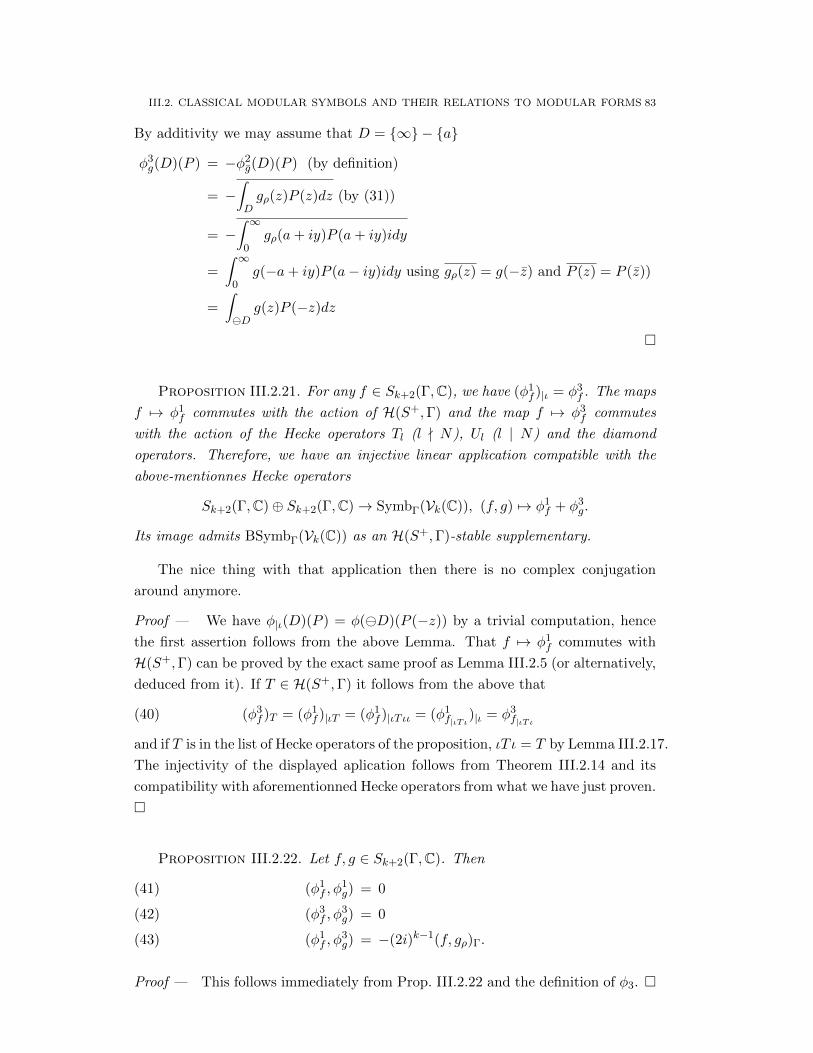
III.2. CLASSICAL MODULAR SYMBOLS AND THEIR RELATIONS TO MODULAR FORMS 83
By additivity we may assume that D = ∞ − a
φ3g(D)(P ) = −φ2
g(D)(P ) (by definition)
= −∫Dgρ(z)P (z)dz (by (31))
= −∫ ∞
0gρ(a+ iy)P (a+ iy)idy
=
∫ ∞0
g(−a+ iy)P (a− iy)idy using gρ(z) = g(−z) and P (z) = P (z))
=
∫D
g(z)P (−z)dz
Proposition III.2.21. For any f ∈ Sk+2(Γ,C), we have (φ1f )|ι = φ3
f . The maps
f 7→ φ1f commutes with the action of H(S+,Γ) and the map f 7→ φ3
f commutes
with the action of the Hecke operators Tl (l - N), Ul (l | N) and the diamond
operators. Therefore, we have an injective linear application compatible with the
above-mentionnes Hecke operators
Sk+2(Γ,C)⊕ Sk+2(Γ,C)→ SymbΓ(Vk(C)), (f, g) 7→ φ1f + φ3
g.
Its image admits BSymbΓ(Vk(C)) as an H(S+,Γ)-stable supplementary.
The nice thing with that application then there is no complex conjugation
around anymore.
Proof — We have φ|ι(D)(P ) = φ(D)(P (−z)) by a trivial computation, hence
the first assertion follows from the above Lemma. That f 7→ φ1f commutes with
H(S+,Γ) can be proved by the exact same proof as Lemma III.2.5 (or alternatively,
deduced from it). If T ∈ H(S+,Γ) it follows from the above that
(φ3f )T = (φ1
f )|ιT = (φ1f )|ιT ιι = (φ1
f|ιT ι)|ι = φ3
f|ιT ι(40)
and if T is in the list of Hecke operators of the proposition, ιT ι = T by Lemma III.2.17.
The injectivity of the displayed aplication follows from Theorem III.2.14 and its
compatibility with aforementionned Hecke operators from what we have just proven.
Proposition III.2.22. Let f, g ∈ Sk+2(Γ,C). Then
(φ1f , φ
1g) = 0(41)
(φ3f , φ
3g) = 0(42)
(φ1f , φ
3g) = −(2i)k−1(f, gρ)Γ.(43)
Proof — This follows immediately from Prop. III.2.22 and the definition of φ3.
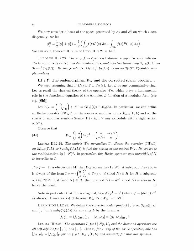
84 III. MODULAR SYMBOLS
We now consider a basis of the space generated by φ1f and φ3
f on which ι acts
diagonally: we let
φ±f =1
2(φ1f ± φ3
f ) =1
2
Å∫Df(z)P (z) dz ±
∫D
f(z)P (−z) dzã.
We can split Theorem III.2.14 or Prop. III.2.21 in half:
Theorem III.2.23. The map f 7→ φf± is a C-linear, compatible with with the
Hecke oprators Tl and Ul and diamondopeators, and injective linear map Sk+2(Γ,C)→Symb±Γ (Vk(C)). Its image admits BSymb±Γ (Vk(C)) as an an H(S+,Γ)-stable sup-
plementary.
III.2.7. The endomorphism WN and the corrected scalar product. .
We keep assuming that Γ1(N) ⊂ Γ ⊂ Γ0(N). Let L be any commutative ring.
Let us recall the classical theory of the operator WN , which plays a fundamental
role in the functional equation of the complex L-function of a modular form (see
e.g. [Shi])
Let WN =
Ç0 1−N 0
å∈ S+ = GL+
2 (Q) ∩M2(Z). In particular, we can define
an Hecke operator [ΓWNΓ] on the spaces of modular forms Mk+2(Γ, L) and on the
spaces of modular symbols SymbΓ(V ) (right V any L-module with a right action
of S+).
Observe that
WN
Ça bc d
åW−1N =
Çd −c/N−Nb a
å.(44)
Lemma III.2.24. The matrix WN normalizes Γ. Hence the operator [ΓWNΓ]
on Mk+2(Γ, L) or SymbΓ(Vk(L)) is just the action of the matrix WN . Its square is
the multiplication by (−N)k. In particular, this Hecke operator acts invertibly if N
is inverible in L.
Proof — It is obvous on (44) that WN normalizes Γ0(N). A subgroup Γ as above
is always of the form ΓH = Ça bc d
å∈ Γ0(p), d (mod N) ∈ H for H a subgroup
of (Z/pnZ)∗. If d (mod N) ∈ H, then a (mod N) = d−1 (mod N) is also in H,
hence the result.
Note in particular that if γ is diagonal, WNγW−1N = γ′ (where γ′ = (det γ)γ−1
as always). Hence for s ∈ S diagonal WN [ΓsΓ]W−1N = [Γs′Γ].
Definition III.2.25. We define the corrected scalar product [ , ]Γ on Sk+2(Γ, L)
and [ , ] on SymbΓ(Vk(L)) for any ring L by the formulas:
[f, g]Γ = (f, g|WN)Γ, [φ1, φ2] = (φ1, (φ2)|WN
)
Lemma III.2.26. The operators Tl for l - Np, Uq and the diamond operators are
all self-adjoint for [ , ]Γ and [ , ]. That is, for T any of the above operator, one has
[f|T , g]Γ = [f, g|T ]Γ for all f, g ∈Mk+2(Γ, L) and similarly for modular symbols.

III.2. CLASSICAL MODULAR SYMBOLS AND THEIR RELATIONS TO MODULAR FORMS 85
Proof — We do the proof for the pairing [ , ]Γ on Mk+2(Γ, L). Write T = [ΓsΓ]
with s ∈ S+. Then
[f|T , g]Γ = (f[ΓsΓ], g|WN)Γ
= (f, g|WN [Γs′Γ])Γ
= [f, g|WN [Γs′Γ]W−1N
]Γ.
Now if T = Tl or Uq we can take s diagonal, so WN [Γs′Γ]W−1N = [ΓsΓ] = T . If
T = 〈a〉 is a diamond operator, a ∈ (Z/NZ)∗, then T = [ΓsΓ] where s is any matrix
in Γ0(N) with lower-right term congruent to a (mod N), and WNs′W−1
N is a matrix
in Γ0(Np) has the same diagonal terms than s, hence WN [Γs′Γ]W−1N = 〈a〉 and the
result follows.
Proposition III.2.27. If f is a newform in Mk+2(Γ,C) then
f|WN= W (f)fρ
where W (f) is a non-zero scalar in the number field Kf (the subfield of C generated
by the coefficients of f) satisfying |W (f)| = Nk.
If f has moreover trivial nebentypus, then f|WN= W (f)f and W (f) = ±Nk/2.
Proof — Write f = q +∑n≥2 anq
n, andlet ε the nebentypus of f . We have seen
that if f is an eigenvector with eigenvalue λ for [ΓsΓ] with s ∈ S+, s diagonal,
then f|WNis an eigenvector for [Γs′Γ] with the same eigenvalue λ. Applyng this for
s =
Çl 00 1
å, l - N , we see that f|Wn
is an eigenvector for Tl = [Γs′Γ] with eigenvalue
the eigenvalue of f for [ΓsΓ], that is alε(l−1). Now the eigenvalue of Tl for fρ is
al wihch is also the eigenvalue of [ΓsΓ] for f using that (f|Tl , f)Γ = (f, f|[ΓsΓ])Γ.
Hence f|Wn= W (f)fρ are proportional since that are newforms. We have (f, f)Γ =
(fρ, fρ)Γ = |W (ρ)|−2(f|WN, f|WN
)Γ = |W (ρ)|−2(f|WNW′N, f)Γ = |W (ρ)|−2Nk(f, f)Γ
using that WNW′N = N Id, hence |W (ρ)| = Nk/2.
Finally, when f has a trivial nebentypus, the eigenvalues for Tl of fρ are just the
al, so f = fρ, and f|WN= W (f)f . Since W 2
N = −N Id acts like the multiplication
by (−N)k, that is Nk since k is even because the nebetypus is trivial, hence W (f) =
±Nk/2
Remark III.2.28. The sign W (f)/Nk/2 is called the root number of f and is
the sign of the functional equation satisfied by L(f, s). See below.
Lemma III.2.29. If f ∈ Sk+2(Γ,C), we have φ1f|WN
= (φ1f )|WN
and φ3f|WN
=
(−1)k(φ3f )|WN
, and we have
[φ+f , φ
−f ] = ik−12k−2Re(f|WN
, fρ)Γ.
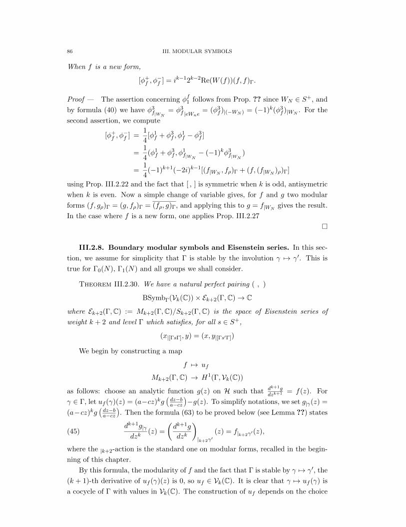
86 III. MODULAR SYMBOLS
When f is a new form,
[φ+f , φ
−f ] = ik−12k−2Re(W (f))(f, f)Γ.
Proof — The assertion concerning φf1 follows from Prop. ?? since WN ∈ S+, and
by formula (40) we have φ3f|WN
= φ3f |eWne
= (φ3f )|(−WN ) = (−1)k(φ3
f )|WN. For the
second assertion, we compute
[φ+f , φ
−f ] =
1
4[φ1f + φ3
f , φ1f − φ3
f ]
=1
4(φ1f + φ3
f , φ1f|WN
− (−1)kφ3f|WN
)
=1
4(−1)k+1(−2i)k−1[(f|WN
, fρ)Γ + (f, (f|WN)ρ)Γ]
using Prop. III.2.22 and the fact that [ , ] is symmetric when k is odd, antisymetric
when k is even. Now a simple change of variable gives, for f and g two modular
forms (f, gρ)Γ = (g, fρ)Γ = (fρ, g)Γ, and applying this to g = f|WNgives the result.
In the case where f is a new form, one applies Prop. III.2.27
III.2.8. Boundary modular symbols and Eisenstein series. In this sec-
tion, we assume for simplicity that Γ is stable by the involution γ 7→ γ′. This is
true for Γ0(N), Γ1(N) and all groups we shall consider.
Theorem III.2.30. We have a natural perfect pairing ( , )
BSymbΓ(Vk(C))× Ek+2(Γ,C)→ C
where Ek+2(Γ,C) := Mk+2(Γ,C)/Sk+2(Γ,C) is the space of Eisenstein series of
weight k + 2 and level Γ which satisfies, for all s ∈ S+,
(x|[ΓsΓ], y) = (x, y|[Γs′Γ])
We begin by constructing a map
f 7→ uf
Mk+2(Γ,C) → H1(Γ,Vk(C))
as follows: choose an analytic function g(z) on H such that dk+1gdzk+1 = f(z). For
γ ∈ Γ, let uf (γ)(z) = (a−cz)kgÄdz−ba−cz
ä−g(z). To simplify notations, we set g|γ(z) =
(a−cz)kgÄdz−ba−cz
ä. Then the formula (63) to be proved below (see Lemma ??) states
dk+1g|γdzk
(z) =
Çdk+1g
dzk
å|k+2γ′
(z) = f|k+2γ′(z),(45)
where the |k+2-action is the standard one on modular forms, recalled in the begin-
ning of this chapter.
By this formula, the modularity of f and the fact that Γ is stable by γ 7→ γ′, the
(k + 1)-th derivative of uf (γ)(z) is 0, so uf ∈ Vk(C). It is clear that γ 7→ uf (γ) is
a cocycle of Γ with values in Vk(C). The construction of uf depends on the choice
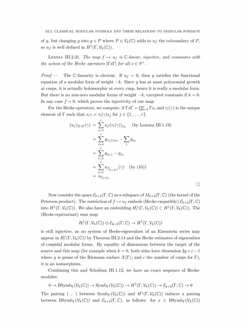
III.2. CLASSICAL MODULAR SYMBOLS AND THEIR RELATIONS TO MODULAR FORMS 87
of g, but changing g into g + P where P ∈ Vk(C) adds to uf the coboundary of P ,
so uf is well defined in H1(Γ,Vk(C)).
Lemma III.2.31. The map f 7→ uf is C-linear, injective, and commutes with
the action of the Hecke operators [ΓsΓ] for all s ∈ S+.
Proof — The C-linearity is obvious. If uf = 0, then g satisfies the functional
equation of a modular form of weight −k. Since g has at most polynomial growth
at cusps, it is actually holomorphic at every cusp, hence it is really a modular form.
But there is no non-zero modular forms of weight −k, excepted constants if k = 0.
In any case f = 0, which proves the injectivity of our map.
For the Hecke operators, we compute, if ΓsΓ =∐ri=1 Γsi and τi(γ) is the unique
element of Γ such that siγ = τi(γ)sj for j ∈ 1, . . . , r.
(uf )|ΓsΓ(γ) =r∑i=1
uf (τi(γ))|si (by Lemma III.1.19)
=r∑i=1
g|τi(γ)si −∑i
g|si
=r∑i=1
g|siγ − g|si
=r∑i=1
uf|k+2si(γ) (by (45))
= uf|ΓsΓ]
Now consider the space Ek+2(Γ,C) as a subspace ofMk+2(Γ,C) (the kernel of the
Peterson product). The restriction of f 7→ uf embeds (Hecke-cmpatibly) Ek+2(Γ,C)
into H1(Γ,Vk(C)). We also have an embedding H1! (Γ,Vk(C)) ⊂ H1(Γ,Vk(C)). The
(Hecke-equivariant) sum map
H1! (Γ,Vk(C))⊕ Ek+2(Γ,C)→ H1(Γ,Vk(C))
is still injective, as no system of Hecke-eigenvalues of an Eisenstein series may
appear in H1! (Γ,Vk(C)) by Theorem III.2.14 and the Hecke estimates of eigenvalues
of cuspidal modular forms. By equality of dimensions between the target of the
source and this map (for example when k = 0, both sides have dimension 2g+ c−1
where g is genus of the Riemann surface X(Γ), and c the number of cusps for Γ),
it is an isomorphism.
Combining this and Scholium III.1.12, we have an exact sequence of Hecke-
modules:
0→ BSymbΓ(Vk(C))→ SymbΓ(Vk(C))→ H1(Γ,Vk(C))→ Ek+2(Γ,C)→ 0
The pairing ( , ) between SymbΓ(Vk(C)) and H1(Γ,Vk(C)) induces a pairing
between BSymbΓ(Vk(C)) and Ek+2(Γ,C), as follows: for x ∈ BSymbΓ(Vk(C))
88 III. MODULAR SYMBOLS
that we see as an element of SymbΓ(Vk(C)) and y ∈ Ek+2(Γ,C), the number
(x, y′) is independent of the lift y′ of y in H1(Γ,Vk(C). To see this, let y′′ be
an other lift, so that y′ − y′′ is the image of an element z in SymbΓ(Vk(C)). But
(x, y−y′) = (x, z) = ±(z, x) and the latter is 0 since the image of x in H1(Γ,Vk(C))
is 0. Obviously then, the pairing between BSymbΓ(Vk(C)) and Ek+2(Γ,C) is perfect.
The proves Theorem III.2.30, since its last assertion follows from Prop. III.2.2.
Exercise III.2.32. Describe a basis of eigenforms for all Hecke operators for
the space BSymbΓ(Vk) when k = 0 and Γ = Γ0(N) where N is a product of r
distinct primes l1, . . . , lr.
Corollary III.2.33. Let us assume that Γ = Γ1(N) for some N and let Hbe the commutative sub-algebra of H(S+,Γ) generated by the Hecke operators Tl
for l a prime not dividing N , Ul for l a prime dividing N and the Diamond op-
erators. Then, as H-modules, BSymbΓ(Vk(C)), Ek+2(Γ,C)∨ and Ek+2(Γ,C)∨ are
isomorphic.
Proof — For l not dividing N , let U ′l be [Γ
Çl 00 1
åΓ]. Let H′ be the commutative
subalgebra of H(S+,Γ) generated by the Tl’s, the U ′l and the Diamond operator.
Fix an isomorphism ψ : H → H′ by sending Tl on Tl, Ul and U ′l and 〈a〉 on 〈a−1〉.Note that in each case ψ sends [ΓsΓ] to [Γs′Γ]. Thus the theorem gives us an
isomorphism of vector spaces Ek+2(Γ,C) → BSymbΓ(Vk(C))∨ which is compatible
with the H′-structure on the source and the H-structure on the target (where H′
is identified with H using ψ).
Now we claim that Ek+2(Γ,C) as an H-module is isomorphic to itself as an
H′-module, when identify H and H′ using ψ. Let W =
Ç1 0−N 0
å. Then a straight-
forward computation shows that f 7→ f|W is an isomorphism of vector spaces of
Ek+2(Γ,C) onto itself, and that (Tf)|W = ψ(T )f|W for any T ∈ H (this is [Mi,
Theorem 4.5.5]), which proves the claim.
Hence we get a genuineH-module isomorphism Ek+2(Γ,C) ' BSymbΓ(Vk(C))∨.
Dualizying, we get Ek+2(Γ,C)∨ ' BSymbΓ(Vk(C)). To conclude, we just recall that
by Corollary ??, Ek+2(Γ,C)∨ ' Ek+2(Γ,C) as H-modules.
Exercise III.2.34. Check directly that SymbΓ0(N)(Vk(V)) ' Ek+2(Γ0(N),C)
as H-modules when k = 0, N a product of distinct primes, using your description
of Exercise III.2.32.
Remark III.2.35. The reader should be warned that while we have constructed
for all N a canonical isomorphism
Ek+2(Γ1(N),C)→ BSymbΓ1(N)(Vk(C))
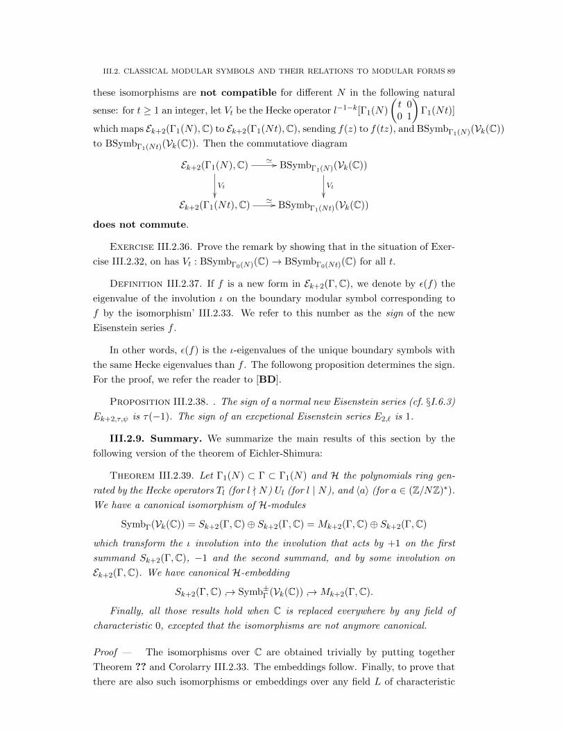
III.2. CLASSICAL MODULAR SYMBOLS AND THEIR RELATIONS TO MODULAR FORMS 89
these isomorphisms are not compatible for different N in the following natural
sense: for t ≥ 1 an integer, let Vt be the Hecke operator l−1−k[Γ1(N)
Çt 00 1
åΓ1(Nt)]
which maps Ek+2(Γ1(N),C) to Ek+2(Γ1(Nt),C), sending f(z) to f(tz), and BSymbΓ1(N)(Vk(C))
to BSymbΓ1(Nt)(Vk(C)). Then the commutatiove diagram
Ek+2(Γ1(N),C)' //
Vt
BSymbΓ1(N)(Vk(C))
Vt
Ek+2(Γ1(Nt),C)' // BSymbΓ1(Nt)(Vk(C))
does not commute.
Exercise III.2.36. Prove the remark by showing that in the situation of Exer-
cise III.2.32, on has Vt : BSymbΓ0(N)(C)→ BSymbΓ0(Nt)(C) for all t.
Definition III.2.37. If f is a new form in Ek+2(Γ,C), we denote by ε(f) the
eigenvalue of the involution ι on the boundary modular symbol corresponding to
f by the isomorphism’ III.2.33. We refer to this number as the sign of the new
Eisenstein series f .
In other words, ε(f) is the ι-eigenvalues of the unique boundary symbols with
the same Hecke eigenvalues than f . The followong proposition determines the sign.
For the proof, we refer the reader to [BD].
Proposition III.2.38. . The sign of a normal new Eisenstein series (cf. §I.6.3)
Ek+2,τ,ψ is τ(−1). The sign of an excpetional Eisenstein series E2,` is 1.
III.2.9. Summary. We summarize the main results of this section by the
following version of the theorem of Eichler-Shimura:
Theorem III.2.39. Let Γ1(N) ⊂ Γ ⊂ Γ1(N) and H the polynomials ring gen-
rated by the Hecke operators Tl (for l - N) Ul (for l | N), and 〈a〉 (for a ∈ (Z/NZ)∗).
We have a canonical isomorphism of H-modules
SymbΓ(Vk(C)) = Sk+2(Γ,C)⊕ Sk+2(Γ,C) = Mk+2(Γ,C)⊕ Sk+2(Γ,C)
which transform the ι involution into the involution that acts by +1 on the first
summand Sk+2(Γ,C), −1 and the second summand, and by some involution on
Ek+2(Γ,C). We have canonical H-embedding
Sk+2(Γ,C) → Symb±Γ (Vk(C)) →Mk+2(Γ,C).
Finally, all those results hold when C is replaced everywhere by any field of
characteristic 0, excepted that the isomorphisms are not anymore canonical.
Proof — The isomorphisms over C are obtained trivially by putting together
Theorem ?? and Corolarry III.2.33. The embeddings follow. Finally, to prove that
there are also such isomorphisms or embeddings over any field L of characteristic

90 III. MODULAR SYMBOLS
0, we only need to consider the case N = Q. In this case, it follows from the
following elementary statement: if M and N are two finite-dimensional Q-vector
spaces privided with an action of a ring H, such that M ⊗ C ' N ⊗ C as C-vector
spaces and H-modules, then M ' N as Q-vector spaces and H-modules. Indeed,
choosing a basis of M and N , a Q-linear application f : M → N is described by its
matrix (xi,j). The fact that f : M → N is an isomorphism, as well as the fact that
it commutes with the action of H are expressed by a system of linear equations
satisfied by the xi,j with coefficients in Q. By hypothesis, this systems has solution
in C. Hence by Gauss’ method it has a solution on Q.
Through the Atkin-Lehner’s theory does not carry over for modular symbols
(cf. Remark ??), many consequences of it carries trivially using the theorem above:
Corollary III.2.40. Let L be any field of characteristic 0. Let H0 be the poly-
nomlials algebras generated by the Tl (l - N) and the diamond operators 〈a〉 (a ∈(Z/NZ)∗). Let λ be a system of eigenvalues H0 → L appearing in Symb±Γ1(N)(Vk(L)).
Then the set of divisors of N such that λ appears in Symb±Γ1(N)(Vk(L)) has a mini-
mal element N0, that we call the minimal level of λ as in the classical Atkin-Lehner’s
tehory (§I.6.3). In particular the notions of λ being new and old, l-new and n-old
make sense. Also, dim Symb±Γ1(N)(Vk(L))[λ] = σ(N/N0).
III.3. Application of classical modular symbols to L-functions and
congruences
III.3.1. Reminder about L-functions. Let f =∑n≥1 anq
n ∈ Sk+2(Γ1(N),C).
Let us recall that the L-function of f is the analytic function L(f, s) =∑n≥1 an/n
s;
the sum converges (absolutely uniformly over all compact) if Re s > k/2 + 2, using
the Hecke’s easy estimate on the an, and actually if Re s > k/2 + 3/2 using the
estimate given by Ramanujan’s generalized conjecture proved by Deligne.
Proposition III.3.1. We have, for Re s > k/2 + 2,∫ ∞0
f(iy)ys−1dy =Γ(s)
(2π)sL(f, s)(46)
Proof — Leaving to the reader the easy arguments justifying the permutation of
the sum and the integral on our domain of convergence , we compute∫ ∞0
f(iy)ys−1dy =∑n>0
∫ ∞0
ane−2πnyys−1dy
=∑n>0
∫ ∞0
an(2πn)s
e−tts−1 dt (change of variable t = 2πny)
=Γ(s)
(2π)s
∑n>0
anns
III.3. APPLICATION OF CLASSICAL MODULAR SYMBOLS TO L-FUNCTIONS AND CONGRUENCES91
Corollary III.3.2. The function L(f, s) has an analytic extension as en entire
holomorphic function over C, and the formula (46) is valid for all s ∈ C.
Proof — Since f(iy) has exponential decay both when y → ∞ and y → 0+,∫∞0 f(iy)ys−1dy converges for all values of s and defines an entire function. Since
Γ(s) has no zero, the results follows.
Corollary III.3.3 (Functional equation). later...
Proof — For the Hecke operator WN defined in §III.2.7, one has f|WN)(z) =
(−1)k
Nzk+2 fÄ−1Nz
ä. Hence Γ(s)
(2π)sL(f|WN, z) = (−1)k
Nik+2
∫∞0
1yk+2 f
ÄiNy
äys−1dy. Make the
change of varables y′ = 1/(Ny). We get Γ(s)(2π)sL(f|WN
, z) = (−1)kNk+2+s
ik+2
∫∞0 yk+1−sf(iy)dy =
(−1)kNk+2+s
ik+2Γ(k+1−s)
(2π)(k+1−s)L(f, k + 1− s). Since f|WN, z) = W (f)L(fρ, z) To be finsi-
hed...
If f is a normalized eigenform for all Hecke operators in Sk+2(Γ1(N), ε), its
L-function has an Euler product:
L(f, s) =∏pN
(1− app−s + ε(p)p1−2s)−1∏p|N
(1− app−s)−1(47)
Slightly more generally, let χ : Z→ C∗ be a Dirichlet character (let us recall that
this means there is a m > 0 such that χ factors as an application χ : Z/mZ→ C∗,with χ(a) = 0 if a 6∈ (Z/mZ)∗, and χ|(Z/mZ)∗ a character. The smallest such d is
called the conductor of χ).
We define the twisted L-function L(f, χ, s) =∑n>0 anχ(n)/ns.
Actually, this L-function may also be seen as the (untwisted) L-function of a
modular form (hence it has an analytic continuation as en entire function as well).
To see this, introduce fχ(z) :=∑n≥1 χ(n)ane
2πinz. Then an easy computation
shows that
fχ(z) =1
τ(χ)
∑a (mod m)
χ(a)f
Åz +
a
m
ã,
where τ(χ) is the Gauss sum∑a(mod m) χ(a)e2iπa/m, and that fχ is a modular form
of level Γ1(Nm).
Exercise III.3.4. Do that computation.
Obviously, L(fχ, s) = L(f, χ, s). Therefore, by the same computation as above:
Lemma III.3.5.
Γ(s)
(2π)sL(f, χ, s) =
1
τ(χ)
∑a (mod m)
χ(a)
∫ ∞0
f(iy + a/m)ys−1dy.
92 III. MODULAR SYMBOLS
As Tate’s thesis showed, the right way to think of L(f, χ, s) is as an extended L-
function of f , in the variable (χ, s). Actually, one can think of (χ, s) as a continuous
character of the idele class group A∗Q/Q∗, with values in C∗ as follows. First χ :
(Z/mZ)∗ → C∗ can be seen as a character of Gal(Q(ζm)/Q) of Gal(Q/Q), that is
by Class Field Theory as a character of A∗Q/Q∗ trivial moreover on R∗+. Or more
directly, using that the inclusion∏l Z∗l ⊂ A∗Q realizes an isomorphism
∏l Z∗l =
A∗Q/Q∗R+∗ , we see χ as a character of
∏l Z∗l , hence of the idele classes, by the
natural surjection∏l Z∗l → (Z/mZ)∗ whose kernel is
∏l 6|m Z∗l ×
∏l|m(1 + lvl(m)Zl).
In any case, we see χ as a character of A∗Q/Q∗ trivial on R∗+. Now we identifies (χ, s)
as the character χ| |s on A∗Q/Q∗. Actually, any continuous character A∗Q/Q∗ → C∗
corresponds this way to one and only one pair (χ, s) where χ is a Dirichlet character
and s ∈ C.
Exercise III.3.6. (easy) Prove the last assertion.
If f is a normalized eigenform for all Hecke operators in Sk+2(Γ1(N), ε), its
L-function has an Euler product:
L(f, χ, s) =∏pN
(1− apχ(p)p−s + ε(p)χ2(p)p1−2s)−1∏p|N
(1− apχ(p)p−s)−1(48)
There is an important basic topic about L(f, s) and L(f, χ, s) that we do not
mention here: the functional equation. See [Shi] for a complete treatment.
III.3.2. Modular symbols and L-functions. We can now use what we have
done to prove a deep arithmetic results about the values of the L-function of a
modular eigenform.
In this §, let Γ = Γ1(N) and let f ∈ Sk+2(Γ) a normalized eigenform for all
the Hecke operators in H. We call λ : H → C be the corresponding character:
Tf = λ(T )f for all T ∈ H.
We recall the modular symbols φ±f ∈ SymbΓ(Vk(C)). Since f 7→ φ±f is H-
equivariant (and C-linear) we have φ±f ∈ Symb±Γ (Vk(C))[λ]. We have more precisely:
Lemma III.3.7. The dimension of Symb±Γ (Vk(C))[λ] is 1
Proof — We have a natural embedding Sk+2(Γ,C)[λ] → Symb±Γ (Vk(C))[λ] whose
cokernel is a direct summand in Ek+2(Γ,C)∨[λ] by Theorem III.2.23 and Corol-
lary ??. But the space Ek+2(Γ,C)[λ] is 0 (hence also Ek+2(Γ,C)∨[λ] since by the
Petersion estimate, there is no Wisenstein series which is an eigenform with the
same eigenvalues as a cuspidal form. And Sk+2(Γ,C)[λ] has dimension 1 by multi-
plicity one (Prop. ??).
Let Kf be the number field generated by the λ(T ), T ∈ H. Then
Lemma III.3.8. The dimension over Kf of Symb±Γ (Vk(Kf ))[λ] is 1

III.3. APPLICATION OF CLASSICAL MODULAR SYMBOLS TO L-FUNCTIONS AND CONGRUENCES93
Proof — Since λ takes values in Kf , this follows form the preceding lemma and
Exercise I.5.5
Definition III.3.9. We define the periods Ω±f of f as the non-zero complex
numbers such that
φ±f /Ω±f ∈ Symb±Γ (Vk(Kf ))[λ].
Obviously, those numbers exists and are well-determine up to multiplication by
an element of K∗f (each of them).
Remark III.3.10. Sometimes we want to work integrally rather than ratio-
nally, and have a smaller indeterminacy on the periods Ω±f . Let Of be the ring
of integer of f . We know that λ(H) ⊂ Of , so Symb±Γ (Vk(Of )][λ] is an Of -
lattice in the 1-dimensional space Symb±Γ (Vk(Kf )][λ]. The minor irritating issue
we are facing is that since Of is a Dedekind domain, but not necessarily principal,
Symb±Γ (Vk(Of ))[λ] might not be free of rank one. It is at any rate projective of
rank one.
When it happens that Symb±Γ (Vk(Of ))[λ] is free of rank one, we can define Ω±fby the requirement that φ±f /Ω
±f is a generator of Symb±Γ (Vk(Of ))[λ]. Thus the
periods Ω±f are well defined up to a unit in O∗f . For example, if f has coefficient
in Q, then Kf = Q, Of = Z which is principal, so Symb±Γ (Vk(Z))[λ] is free of rank
one, and the periods Ω±f are well defined up to a sign.
When Symb±Γ (Vk(Of ))[λ] is not free, we have several solutions, depending on
what we want to do. For example we can replace Kf by a finite extension K ′ on
which this module becomes free (for example, the Hilbert Class Field of Kf will
do), and have Ω±f well defined up to an element in O∗K′ . Or we can work at one
prime at a time: for p a prime of Of , the localization Of,(p) is principal, so it is
possible to require that Ω±f is chosen such that φ±f /Ω±f is in Symb±Γ (Vk(Of ))[λ],
and generates that module after localizing at p. Such a requirement fixes Ω±f up to
multiplication by an element of K∗p whose p-valuation is 0, which is often sufficient
in the applications. When Ω± is chosen this way, we shall say that it is p-normalized
(that’s our terminology, not a standard one).
Theorem III.3.11 (Manin-Shokurov). For any Dirichlet character χ, any in-
teger j such that 0 ≤ j ≤ k, we have
L(f, χ, j + 1)
Ω±f (iπ)j+1∈ Kf [χ],
where the sign ± is chosen such that ±1 = (−1)jχ(−1), and Kf [χ] is the extension
of Kf generated by the image of χ.

94 III. MODULAR SYMBOLS
Proof — We have for j an integer, 0 ≤ j ≤ k,∫ ∞0
f(iy + a/m)yidy = i−j−1∫ ∞a/m
f(z)(z − a/m)jdz
= i−j−1φ1f (∞− a/m)((z − a/m)j).
Hence using Lemma III.3.5,
Γ(j + 1)ij+1τ(χ)
(2π)j+1L(f, χ, j + 1) =
∑a (mod m)
χ(a)φ1f (∞ − a/m)((z − a/m)j)
We note that the right hand side is multiplied by (−1)jχ(−1) if the occurrence of
φ1f in it is replaced by (φ1
f )|ι. Hence we can replace φ1f by φ±f with ±1 = (−1)jχ(−1)
in that formula. We thus have
j!τ(χ)
(−2iπ)j+1Ω±fL(f, χ, j + 1) =
∑a (mod m)
χ(a)φ±f (∞ − a/m)((z − a/m)j)
Ω±f(49)
and the results follows from Definition III.3.9.
Exercise III.3.12. Let p be a prime of Of and assume that Ω± is p-normalized
(notations of Remark III.3.10). Show that the numbers j!τ(χ)
(−2iπ)j+1Ω±f
L(f, χ, s) (when
0 ≤ j ≤ k, χ is a Dirichlet character, and χ(−1)(−1)j = ±1) are p-integers if the
conductor m of χ is prime to p. Show also that when k = 0, at least one of those
number has p-valuation 0.
III.3.3. Scalar product and congruences. In this paragraph, we present
as an application a weak version of a nice theorem of Hida (cf. [H1] and [H2]).
We continue to assume Γ = Γ1(N). Let f be a newform in Sk+2(Γ,C).
Proposition III.3.13. One has
[φ+f , φ
−f ] = −4W (f)(−i)k−1(f, f)Γ
and the number (f, f)Γ/(ik−1Ω+
f Ω−f ) belongs to Kf . One has [φ+f , φ
+f ] = [φ−f , φ
−f ] =
0
Proof — By (43), one has
(φ1f , φ
3fρ) = (φ1
f , φ2f ) = −2ik−1(f, f)Γ.(50)
Applying this to fρ, one also has
(φ1fρ , φ
3f ) = −2ik−1(f, f)Γ(51)
since obviously (f, f)Γ = (fρ, fρ)Γ. Recall also that one has, for any f, g,
(φ1f , φ
1g) = (φ3
f , φ3g) = 0.(52)
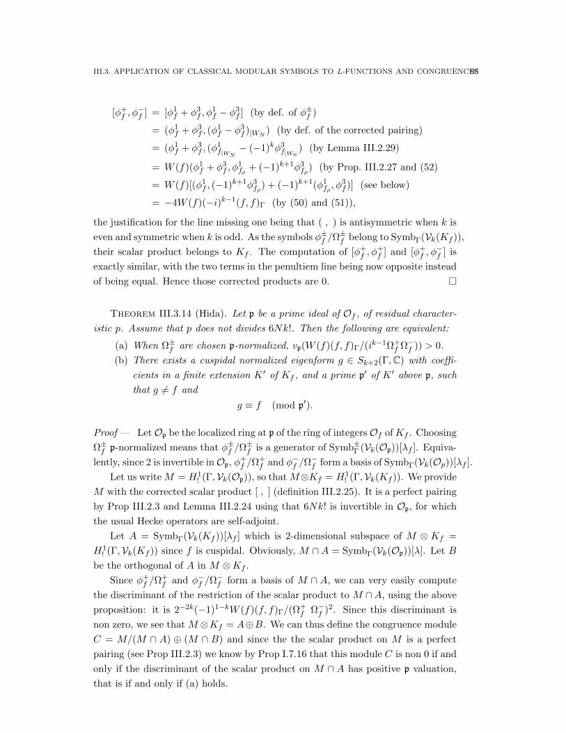
III.3. APPLICATION OF CLASSICAL MODULAR SYMBOLS TO L-FUNCTIONS AND CONGRUENCES95
[φ+f , φ
−f ] = [φ1
f + φ3f , φ
1f − φ3
f ] (by def. of φ±f )
= (φ1f + φ3
f , (φ1f − φ3
f )|WN) (by def. of the corrected pairing)
= (φ1f + φ3
f , (φ1f|WN
− (−1)kφ3f|Wn
) (by Lemma III.2.29)
= W (f)(φ1f + φ3
f , φ1fρ + (−1)k+1φ3
fρ) (by Prop. III.2.27 and (52)
= W (f)[(φ1f , (−1)k+1φ3
fρ) + (−1)k+1(φ1fρ , φ
3f )] (see below)
= −4W (f)(−i)k−1(f, f)Γ (by (50) and (51)),
the justification for the line missing one being that ( , ) is antisymmetric when k is
even and symmetric when k is odd. As the symbols φ±f /Ω±f belong to SymbΓ(Vk(Kf )),
their scalar product belongs to Kf . The computation of [φ+f , φ
+f ] and [φ+
f , φ−f ] is
exactly similar, with the two terms in the penultiem line being now opposite instead
of being equal. Hence those corrected products are 0.
Theorem III.3.14 (Hida). Let p be a prime ideal of Of , of residual character-
istic p. Assume that p does not divides 6Nk!. Then the following are equivalent:
(a) When Ω±f are chosen p-normalized, vp(W (f)(f, f)Γ/(ik−1Ω+
f Ω−f )) > 0.
(b) There exists a cuspidal normalized eigenform g ∈ Sk+2(Γ,C) with coeffi-
cients in a finite extension K ′ of Kf , and a prime p′ of K ′ above p, such
that g 6= f and
g ≡ f (mod p′).
Proof — LetOp be the localized ring at p of the ring of integersOf ofKf . Choosing
Ω±f p-normalized means that φ±f /Ω±f is a generator of Symb±Γ (Vk(Op))[λf ]. Equiva-
lently, since 2 is invertible inOp, φ+f /Ω
+f and φ−f /Ω
−f form a basis of SymbΓ(Vk(Op))[λf ].
Let us write M = H1! (Γ,Vk(Op)), so that M⊗Kf = H1
! (Γ,Vk(Kf )). We provide
M with the corrected scalar product [ , ] (definition III.2.25). It is a perfect pairing
by Prop III.2.3 and Lemma III.2.24 using that 6Nk! is invertible in Op, for which
the usual Hecke operators are self-adjoint.
Let A = SymbΓ(Vk(Kf ))[λf ] which is 2-dimensional subspace of M ⊗ Kf =
H1! (Γ,Vk(Kf )) since f is cuspidal. Obviously, M ∩ A = SymbΓ(Vk(Op))[λ]. Let B
be the orthogonal of A in M ⊗Kf .
Since φ+f /Ω
+f and φ−f /Ω
−f form a basis of M ∩ A, we can very easily compute
the discriminant of the restriction of the scalar product to M ∩A, using the above
proposition: it is 2−2k(−1)1−kW (f)(f, f)Γ/(Ω+f Ω−f )2. Since this discriminant is
non zero, we see that M ⊗Kf = A⊕B. We can thus define the congruence module
C = M/(M ∩ A) ⊕ (M ∩ B) and since the the scalar product on M is a perfect
pairing (see Prop III.2.3) we know by Prop I.7.16 that this module C is non 0 if and
only if the discriminant of the scalar product on M ∩ A has positive p valuation,
that is if and only if (a) holds.

96 III. MODULAR SYMBOLS
But on the other hand, the fact that the congruence module C is non-zero is
equivalent (cf. Prop. I.7.15) to the existence of a modular symbol φ′ in B such
that φ′ ≡ aφ+f + bφ−f (mod p), with a, b ∈ Op, not both in p. By Deligne-Serre’s
lemma (up to allowing finite extension K ′ of Kf and replacement of p be a prime
p′ of K ′ dividing p) this is equivalent to the same thing with φ′ assume to be
an eigenvector for all Hecke operators. Such an eigenvector φ′ defines a cuspidal
normalized eigenform g ∈ Sk+2(Γ,K ′) with the same Hecke eigenvalues. Hence C is
non-zero if and only if there exists a cuspidal normalized eigenform g whose Hecke
eigenvalues are congruent to those of f . In our case, this is also equivalent to g ≡ f(mod p), for the two residual form g mod p and f (mod p) in Sk+2(Γ,Op/p) will
have the same eigenvalues, hence the same Fourier coefficients, hence will be equal
by the q-development principle.
In other words, C 6= 0 is equivalent to (b). This proves the theorem.
III.4. Distributions
In all this section, L will denote a commutative noetherian Qp-Banach algebra
(as in [Bu]) with a norm denoted | | extending the usual absolute value on Qp, so
that |p| = 1/p.
III.4.1. Some modules of sequences and their dual. For L any commu-
tative Qp-algebra, and r any positive real number, we shall denote by cr(L) (resp.
br(L)) the Banach L-module of sequences (an)n≥0, with an ∈ L and |an|rn →0 when n → ∞ (resp. with |an|rn bounded above), with the norm |(an)| =
supn≥0 |an|rn. When r = 1, we shall denote c(L) for c1(L) (resp. b(L) for b1(L)).
Note that the Cauchy product makes cr(L) and br(L) Banach algebras over L.
Lemma III.4.1. The natural map cr(Qp)⊗QpL → cr(L) is an isometry, and is
compatible with the L-algbera structure. In particular, for any continuous morphism
L → L′ of Qp-Banach algebras, we have an isomorphism cr(L)⊗LL′ = cr(L′) of
L′-Banach algebras.
Proof — The first statement is proved exactly as [BGR, Prop 2.1.7/8]. The
second folloews from the first and the associativity of completed tensor product.
Lemma III.4.2. If there is an R in L∗ with |R| = r and |R−1| = r−1, then there
are isometric isomorphisms of L-algebras cr(L) ' c(L) and br(L) ' b(L).
Proof — Since |R−1| = |R|−1, the element R is multiplicative ([BGR, Prop.
1.2.2/4]), that is |anRn| = |an||R|n = |an|rn. Hence we can define a map cr(L) →c(L) that sends (an) to (anR
n). It is obviously an isometric isomorphism of algebras.
Same proof for br(L) and b(L).

III.4. DISTRIBUTIONS 97
Lemma III.4.3. The Banach L-module cr(L) is always potentially ON-able. If
there is an element R ∈ L∗ such that |R| = r and |R−1| = r−1, then A[r](L) is
actually ON-able.
Proof — The Qp-Banach space cr(Qp) is potentially ONable as is any Qp-Banach
space by [S]. Then the L-Banach module
cr(L) = cr(Qp)⊗QpL
is potentially ONable by [Bu, Lemma 2.8]. The second assertion follows from
Lemma III.4.2 since c(L) is ON-able by definition.
Exercise III.4.4. (easy) Show that cp1/2(Qp) is not ON-able.
Lemma III.4.5. There are natural isometric isomorphisms of Banach L-modules
b 1r(L) = HomL(cr(L), L) = HomQp(cr(Qp), L)(53)
Proof — if b = (bn)n∈N ∈ b 1r(L), one defines an L-linear form lb on cr(L) by
setting lb((an)) =∑n anbn. The sum converges since |an|rn goes to 0 and |bn|/rn
is bounded, so anbn goes to 0. The operator norm of lb is clearly |b|. Conversely,
any continuous linear form l on c(L) defines a sequence b = (bn) by setting bn =
l((δn,m)m≥0) where δm,n is Kronecker’s symbol, and that sequence is bounded by
the operator of norm of l. One checks immediately that l = lb. This proves the
first isomorphisms. The second is proved the same way.
Let us define a Banach L-module b′r(L) as br(Qp)⊗QpL. The map br(Qp) ⊂ b(L)
induces an injective norm-preserving b′r(L) → br(L), which allows us to see b′r(L)
as a closed submodule of br(L) with the induced norm. Using lemma III.4.5, one
can also seen b′1r
(L) as a closed submodule of HomQp(cr(Qp), L).
Proposition III.4.6. The sub-module b′1r
(L) of HomQp(cr(Qp), L) contains ex-
actly the linear applications from cr(Qp) to L that are comapct (that is, completely
continuous).
Proof — [S, Corollary, page 74]
Corollary III.4.7. The inclusion b′r(L) ⊂ br(L) is proper if and only if L is
infinite-dimensional over Qp.
Proof — If L is finite-dimensional, every linear map in HomQp(cr(Qp), L) has
finite rank hence is compact. If L is infinite-dimensional, there are linear maps in
HomQp(cr(Qp), L) that are non-compact.
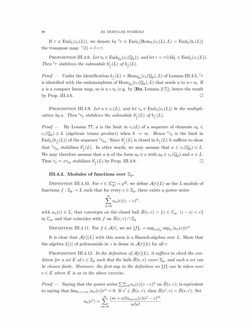
98 III. MODULAR SYMBOLS
If τ ∈ EndL(cr(L)), we denote by tτ ∈ EndL(HomL(cr(L), L) = EndL(br(L))
the transpose map: τ (l) = l τ .
Proposition III.4.8. Let τ0 ∈ EndQp(cr(Qp)), and let τ = τ⊗IdL ∈ EndL(cr(L)).
Then tτ stabilizes the submodule b′1r
(L) of b 1r(L).
Proof — Under the identification b 1r(L) = HomQp(cr(Qp), L) of Lemma III.4.5, tτ
is identified with the endomorphism of HomQp(cr(Qp), L) that sends u to u τ0. If
u is a compact linear map, so is u τ0 (e.g. by [Bu, Lemma 2.7]), hence the result
by Prop. III.4.6.
Proposition III.4.9. Let a ∈ cr(L), and let τa ∈ EndL(cr(L)) be the multipli-
cation by a. Then tτa stabilizes the submodule b′1r
(L) of b 1r(L).
Proof — By Lemma ??, a is the limit in cr(L) of a sequence of elements ak ∈cr(Qp) ⊗ L (algebraic tensor product) when k → ∞. Hence tτa is the limit in
EndL(b 1r(L)) of the sequence tτak . Since b′1
r
(L) is closed in b 1r(L) it suffices to show
that tτak stabilizes b′1r
(L). In other words, we may assume that a ∈ cr(Qp) ⊗ L.
We may therefore assume that a is of the form a0 ⊗ x with a0 ∈ cr(Qp) and x ∈ L.
Thus τa = xτa0 stabilizes b′1r
(L) by Prop. III.4.8.
III.4.2. Modules of functions over Zp.
Definition III.4.10. For r ∈ |C∗p| = pQ, we define A[r](L) as the L-module of
functions f : Zp → L such that for every e ∈ Zp, there exists a power series∞∑n=0
an(e)(z − e)n,
with an(e) ∈ L, that converges on the closed ball B(e, r) = z ∈ Cp, |z − e| < rin Cp, and that coincides with f on B(e, r) ∩ Zp
Definition III.4.11. For f ∈ A[r], we set ||f ||r = supe∈Zp supn |an(e)|rn
It is clear that A[r](L) with this norm is a Banach-algebra over L. Show that
the algebra L[z] of polynomials in z is dense in A[r](L) for all r.
Proposition III.4.12. In the definition of A[r](L), it suffices to check the con-
dition for a set E of e ∈ Zp such that the balls B(e, r) cover Zp, and such a set can
be chosen finite. Moreover, the first sup in the definition on ||f || can be taken over
e ∈ E where E is as in the above exercise.
Proof — Saying that the power series∑∞n=0 an(e)(z− e)n on B(e, r), is equivalent
to saying that limn→+∞ |an(e)|rn = 0. If e′ ∈ B(e, r), then B(e′, r) = B(e, r). Set
an(e′) =∞∑m=0
(m+ n)!am+n(e)(e′ − e)m
m!n!
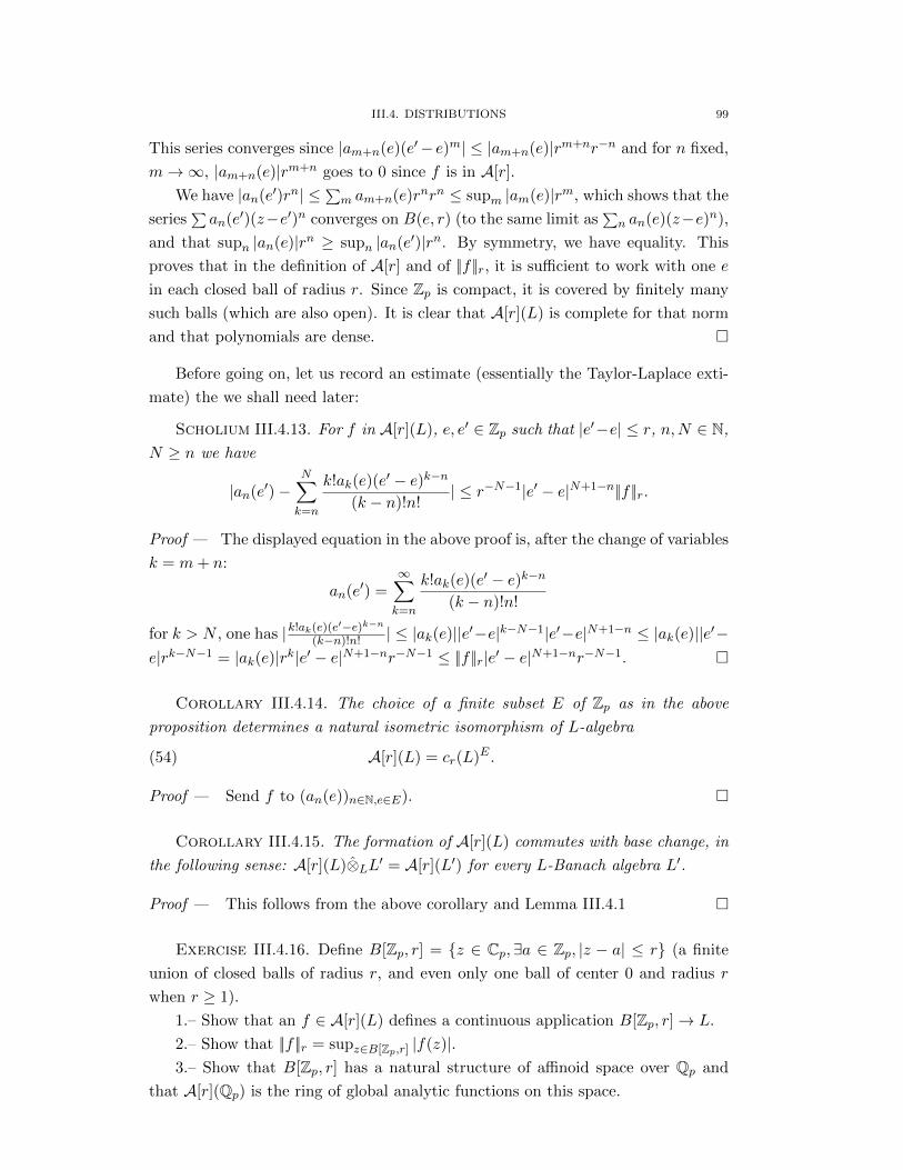
III.4. DISTRIBUTIONS 99
This series converges since |am+n(e)(e′− e)m| ≤ |am+n(e)|rm+nr−n and for n fixed,
m→∞, |am+n(e)|rm+n goes to 0 since f is in A[r].
We have |an(e′)rn| ≤∑m am+n(e)rnrn ≤ supm |am(e)|rm, which shows that the
series∑an(e′)(z−e′)n converges on B(e, r) (to the same limit as
∑n an(e)(z−e)n),
and that supn |an(e)|rn ≥ supn |an(e′)|rn. By symmetry, we have equality. This
proves that in the definition of A[r] and of ||f ||r, it is sufficient to work with one e
in each closed ball of radius r. Since Zp is compact, it is covered by finitely many
such balls (which are also open). It is clear that A[r](L) is complete for that norm
and that polynomials are dense.
Before going on, let us record an estimate (essentially the Taylor-Laplace exti-
mate) the we shall need later:
Scholium III.4.13. For f in A[r](L), e, e′ ∈ Zp such that |e′−e| ≤ r, n,N ∈ N,
N ≥ n we have
|an(e′)−N∑k=n
k!ak(e)(e′ − e)k−n
(k − n)!n!| ≤ r−N−1|e′ − e|N+1−n||f ||r.
Proof — The displayed equation in the above proof is, after the change of variables
k = m+ n:
an(e′) =∞∑k=n
k!ak(e)(e′ − e)k−n
(k − n)!n!
for k > N , one has |k!ak(e)(e′−e)k−n(k−n)!n! | ≤ |ak(e)||e′−e|k−N−1|e′−e|N+1−n ≤ |ak(e)||e′−
e|rk−N−1 = |ak(e)|rk|e′ − e|N+1−nr−N−1 ≤ ||f ||r|e′ − e|N+1−nr−N−1.
Corollary III.4.14. The choice of a finite subset E of Zp as in the above
proposition determines a natural isometric isomorphism of L-algebra
A[r](L) = cr(L)E .(54)
Proof — Send f to (an(e))n∈N,e∈E).
Corollary III.4.15. The formation of A[r](L) commutes with base change, in
the following sense: A[r](L)⊗LL′ = A[r](L′) for every L-Banach algebra L′.
Proof — This follows from the above corollary and Lemma III.4.1
Exercise III.4.16. Define B[Zp, r] = z ∈ Cp,∃a ∈ Zp, |z − a| ≤ r (a finite
union of closed balls of radius r, and even only one ball of center 0 and radius r
when r ≥ 1).
1.– Show that an f ∈ A[r](L) defines a continuous application B[Zp, r]→ L.
2.– Show that ||f ||r = supz∈B[Zp,r] |f(z)|.3.– Show that B[Zp, r] has a natural structure of affinoid space over Qp and
that A[r](Qp) is the ring of global analytic functions on this space.
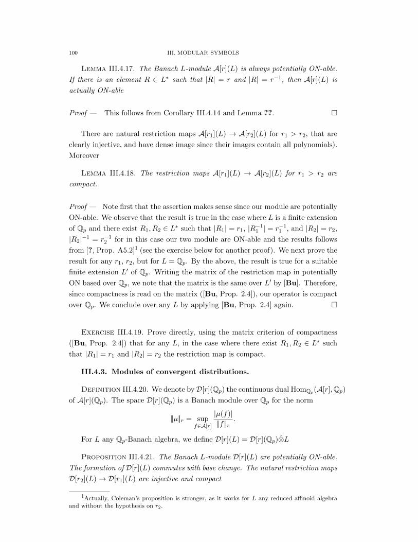
100 III. MODULAR SYMBOLS
Lemma III.4.17. The Banach L-module A[r](L) is always potentially ON-able.
If there is an element R ∈ L∗ such that |R| = r and |R| = r−1, then A[r](L) is
actually ON-able
Proof — This follows from Corollary III.4.14 and Lemma ??.
There are natural restriction maps A[r1](L) → A[r2](L) for r1 > r2, that are
clearly injective, and have dense image since their images contain all polynomials).
Moreover
Lemma III.4.18. The restriction maps A[r1](L) → A[r2](L) for r1 > r2 are
compact.
Proof — Note first that the assertion makes sense since our module are potentially
ON-able. We observe that the result is true in the case where L is a finite extension
of Qp and there exist R1, R2 ∈ L∗ such that |R1| = r1, |R−11 | = r−1
1 , and |R2| = r2,
|R2|−1 = r−12 for in this case our two module are ON-able and the results follows
from [?, Prop. A5.2]1 (see the exercise below for another proof). We next prove the
result for any r1, r2, but for L = Qp. By the above, the result is true for a suitable
finite extension L′ of Qp. Writing the matrix of the restriction map in potentially
ON based over Qp, we note that the matrix is the same over L′ by [Bu]. Therefore,
since compactness is read on the matrix ([Bu, Prop. 2.4]), our operator is compact
over Qp. We conclude over any L by applying [Bu, Prop. 2.4] again.
Exercise III.4.19. Prove directly, using the matrix criterion of compactness
([Bu, Prop. 2.4]) that for any L, in the case where there exist R1, R2 ∈ L∗ such
that |R1| = r1 and |R2| = r2 the restriction map is compact.
III.4.3. Modules of convergent distributions.
Definition III.4.20. We denote byD[r](Qp) the continuous dual HomQp(A[r],Qp)
of A[r](Qp). The space D[r](Qp) is a Banach module over Qp for the norm
||µ||r = supf∈A[r]
|µ(f)|||f ||r
.
For L any Qp-Banach algebra, we define D[r](L) = D[r](Qp)⊗L
Proposition III.4.21. The Banach L-module D[r](L) are potentially ON-able.
The formation of D[r](L) commutes with base change. The natural restriction maps
D[r2](L)→ D[r1](L) are injective and compact
1Actually, Coleman’s proposition is stronger, as it works for L any reduced affinoid algebraand without the hypothesis on r2.
III.4. DISTRIBUTIONS 101
Proof — The Banach D[r](Qp) is potentially orthonormalizable by [S]. It is
clear by definition that the formation of D[r](L) commute with base change. The
transposed restriction maps D[r2](Qp) → D[r1](Qp) are obviously injective since
the restriction maps A[r1](Qp) → A[r2](Qp) have dense image (since their im-
ages contain polynomials). They are compact, since the transpose of a compact
map is compact (see [S, Lemma 14] or [Sch, Lemma 16.4]). The restriction maps
D[r2](L) → D[r1](L) are defined by base change from the case L = Qp, so their
injectivity and compactness follow.
We note that the we have a natural injective norm-preserving map D[r](L) =
D[r](Qp)⊗L→ HomL(A[r](L), L) which identified D[r](L) as a closed subspace of
HomL(A[r](L), L). The following lemma is obvious form the definitions.
Lemma III.4.22. Let E be as in Prop. III.4.12. Then through the isomorphisms
(54) and (??)
HomL(A[r](L), L) = HomL(cr(L)E , L) = b 1r(L)E
the subspace D[r](L) of HomL(A[r](L), L) is identified with the subspace b′1r
(L)E of
b 1r(L)E.
In particular, we see that D[r](L) is strictly smaller than the L-dual of A[r](L)
when L is not finite-dimensional over Qp. This is the price to pay to have a
D[r](L) whose formation commute with base change, which will be crucial for the
application to the eigencurve below.
III.4.4. Modules of overconvergent functions and distributions.
Definition III.4.23. For r ≥ 0, we define the modules of overconvergent func-
tions
A†[r](L) = lim−→
r′>r,r′∈pQA[r′](L) =
⋃r′>r
A[r′](L).
The module A†[0](L) is simply the module of L-valued locally analytic functions
on Zp: functions that around every point e admit a converging Taylor expansion
on some ball of some positive radius r depending on e. The module A†[1] is the
module of analytic functions on Zp defined by a powers series that converges ”a
little bit more than necessary”, that is on some ball of center 0 and radius r > 1.
When L is a finite extension of Qp, we shall need to give a topology on A†[r](L):
we give it the locally convex final topology (see [Sch, §5.E]), that is the finest locally
convex topology such that the natural morphism A[r′](L) → D†[r](L) for r′ > r
are continuous.
Definition III.4.24. For any r ≥ 0, we set
D†[r](L) = lim←−
r′>r, r′∈pQD[r′](L).
102 III. MODULAR SYMBOLS
In other words D†[r](L) is the intersection of the D[r′](L) for r′ > r.
We give those modules the topology of the projective limit. In other words, the
topology of D†[r](L) is defined by the family of norms ||µ||r′ for all r′ > r, r′ ∈ pQ.
It is clear that D†[r](L) is complete for that topology.
In proposition below the notion of completed tensor product of two Frechet
spaces over Qp, which is introduced in [Sch, §17], cf. in particular [Sch, Prop.
17.6]. Let us briefly recall that if V and W are two locally convex spaces over
Qp, then one can define on V ⊗ W two natural locally convex topologies: the
inductive topology (resp. projective topology) is the finest one that makes the map
V ×W → V ⊗W separately (resp. jointly) continuous. The projective topology is
also the one defines by the semi-norms p⊗q, where p (resp. q) runs among a family
of semi-norms defining the topology of V (resp. of W ), and p⊗ q is the semi-norm
of V ⊗W defined by p ⊗ q(x) = infx=∑
vi⊗wi supi p(vi)q(wi), for all x ∈ V ⊗W ,
the inf being taken on all the writing x =∑i vi⊗wi with the vi’s in V , the wi’s in
W . Then [Sch, Prop. 17.6] proves that if V and W are Frechet, the completion of
V ⊗W for both those topology coincides. This is this completion that is denoted
by V ⊗W .
We shall need repeatedly the following observation, where for V a locally convex
space, we denote by c(V ) the locally convex space of sequences (vn)n≥0 of elements
of V that converge to 0: if V is a Frechet, then c0(Qp)⊗V is naturally isomorphic
to the Frechet space c0(V ). Indeed, one sees immediately that the obvious map
c0(Qp) × V → c0(V ) is separately continuous, and has dense image, hence an
isomorphism between the completion of c0(Qp)⊗ V and c0(V ).
Proposition III.4.25. For any Banach algebra L, we have a natural isomor-
phism of Frechet spaces D†[r](Qp)⊗L→ D†[r](L).
Proof — The maps D†[r]⊗L → D[r′]⊗L for r′ > r induces an injective map
D†[r]⊗L → proj limr′>r D[r′](L) = D†[r](L). This map is obviously an isomor-
phism when L is finite over Qp. Otherwise since L is potentially orthonormalizable,
we can choose an isomorphism L ' c(Qp) and by the above observation, we only
need to prove that the natural map c(D†[r])→ proj limr′>r c(D[r′]) = ∩r′>rc(D[r′])
is an isomorphism, which is clear since a sequence (vn) in D†[r] goes to 0 if and
only if ||vn||r′ goes to 0 for all r′ > r.
For the next corollary, we shall need the notion of the completed tensor product,
over a Banach algebra L, of a Banach module W and of a module V is defined by a
family of semi-norms. Unfortunately, this notion is not covered in either of our two
basic references in non-archimedean analysis, [BGR] (which consider only Banach
modules over a Banach algebra, with topology defined by one norm), or [Sch] which
considers completed tensor products over a field, never over a ring. We shall defined
III.4. DISTRIBUTIONS 103
V ⊗LW as follows: if p is a norm defining the topology of W , and (qi) are the semi-
norms defining the topology of V , we put on V ⊗L W the family of semi-norms
(qi ⊗ p), and we define V ⊗RW as the completion of V ⊗LW for that topology. It
is cleat thai if L = Qp, the topology we have defines on V ⊗W is the projective
topology, hence our notion of V ⊗QpW coincide with theone defined in [Sch] and
recalled above. If W = L′ is a Banach algebra, whose L-module structure is a
continious morphism of Banach algebra L→ L′, then V ⊗LL′ is an L′-module and
the semi-norms (qi⊗p) are norm of L′-modules. We can thus, if L′ → L′′ is another
morphism of Banach algebras, consided (V ⊗LL′)⊗L′L′′. One sees easily that this
may be identified with V ⊗LL′′. This, with Prop. III.4.25, immediately gives:
Corollary III.4.26. For any morphism L → L′ of Banach algebras, we have
a natural isomorphism of topological module overL′:
D†[r](L)⊗LL′ = D†[r](L′)
Let us also note:
Proposition III.4.27. Assume that L is a finite extension of Qp. Then that
family of norms makes D†[r](L) a Frechet vector space over L. Moreover, D†[r](L)
may be canonically identified, as a topological vector space, to the continuous dual
(with its strong topology) of A†[r](L) with its locally convex inductive limit topology.
Proof — Remember that A†[r](L) = lim ←−r′>rA[r′](L) by definition, where the
transition maps are injective and compact (Prop. ??), and that the dual of A[r′](L)
with its operator norm (that is, its strong dual, cf. [Sch, Remark 6.7]) is D[r′](L).
We can therefore apply directly [Sch, Prop 16.10], whose points ii. and iii. are
exactly what we want.
Let L be a finite extension of Qp. If f ∈ A[r](L) or f ∈ A†[r](L), and µ ∈D[r](L) or D†[r](L), we have by definition or by the above proposition a scalar
µ(f) ∈ L. We will sometimes use the following longer but intuitive notation:∫Zpf(z)dµ(z) := µ(f).
Slightly more generally, for a ∈ Zp and n ∈ N, we set∫a+pnZp
f(z)dµ(z) :=
∫Zpf(z)1a+pnZp(z)dµ(z) = µ(f1a+pnZp).
We shall refer to the modules D[r] and D†[r] as modules of distributions over
Zp, even if properly speaking only D†[0] (the continuous dual of the space A†[0] of
locally analytic functions) is the real module of distributions over Zp.
To simplify notations, we shall henceforth write D in-stead of D†[0]

104 III. MODULAR SYMBOLS
III.4.5. Order of growth of a distribution.
Definition III.4.28. Let ν ≥ 0 be a real number. We say that a distribution
µ ∈ D has order ≤ ν if there exists a constant C ∈ R+ such that for all a in Zp,k, n ∈ N, we have ∣∣∣∣∣
∫a+pnZp
(z − apn
)kdµ(z)
∣∣∣∣∣ < Cpnν .(55)
A distribution of order ≤ 0 is called a measure on Zp. A distribution which is of
order ≤ ν for some ν is called a tempered distribution.
Remark III.4.29. Visik ([V]) and Colmez ([CO1]) use an intersting equivalent
definition for ν an integer: a distribution µ is of order ν ∈ N if, as a continuous
linear form on the space A†[0] of locally analytic functions on Zp, it extends to the
larger space of class Cν , defined as the space of functions that admits N -derivative
and such that the last-derivative is Lipschitz. We shall not use this defintion.
There is an easy characterization of the order of growth in terms of norms:
Lemma III.4.30. Let µ ∈ D(L) be a distribution. Then µ has order ≤ ν if and
only if there exists a real D > 0 such that ||µ||r ≤ Dr−ν when r → 0+. Moreover,
we can take D = Cp if C is as in (55).
Proof — Note that ga,n,k(z) := ( z−apn )k1a+pnZp(z) satisfies ||ga,n,k||r = 1 for r = p−n.
Thus if ||µ||r ≤ Dr−ν for all r, we get for r = p−n that |µ(ga,n,k)| ≤ Dpnν and µ has
order of growth ≤ ν.
For the converse, let µ have order of growth ≤ ν. Then there is a C such
that∣∣∣∫a+pnZp(
z−apn )kdµ(z)
∣∣∣ < Cpnν . Let f ∈ A[p−n], and e ∈ Zp. Write the
power series of f about e as f(z) =∑∞k=0 ak(e)p
−nk(z − e)k. Then ||f ||p−n =
supe∈E supk |ak(e)p−nk|p−nk = supe∈E supk∈N |ak(e)|, where E is a finite subset of
Zp as in Prop. III.4.12. Then
µ(f) =∑e∈E
∞∑k=0
ak(e)
∫a+pnZp
(z − apn
)kdµ(z)
so |µ(f)| ≤ ||f ||p−nCpnν .
Now if r is a positive real number, r < 1, there is an n ∈ N such that p−n <
r ≤ p−n+1, and we have |µ(f)| ≤ ||f ||p−nCpnν ≤ ||f ||rCpr−ν , that is ||µ||r ≤ Dr−ν
with D = Cp.
Theorem III.4.31 (Vishik, Amice-Velu). Let L be a finite extension of Qp
(i) Let µ ∈ D(L) a distribution of order ≤ ν, and let N be an integer grater
or equal to the integral part of ν. Then µ is uniquely determined by the

III.4. DISTRIBUTIONS 105
linear forms for a ∈ Zp and n ∈ N:
iµ,a+pnZp : PN (L) → L
P 7→∫a+pnZp
P (z)dµ(z).
Here as above, PN (L) is the finite-dimensional space of polynomials of
degree less than N over L.
(ii) Conversely, suppose we are given, for every ball a + pnZp in Zp, a linear
form ia+pnZp : PN (L)→ L which satisfy the natural additivity relation
(for all a ∈ Zp, n ∈ N)
ia+pnZp =p−1∑i=0
ia+pni+pn+1Zp ,(56)
and such that there exist constants C > 0 and ν ≥ 0 such that for every
a ∈ Zp, k, n ∈ N, and k ≤ N
|ia+pnZp((z − apn
)k)| ≤ Cpnν .(57)
Then there exists a (unique) distribution µ of order ≤ ν such that iµ,a+pnZp =
ia+pnZp, and for any n ∈ N one has
||µ||p−n ≤ Cpnν .
This theorem is not hard to prove, just a little bit computational. It says that
a distribution on order ν is known when you know how it integrates polynomials
of degree less or equal than bνc on closed balls in Zp, and conversely, that any way
to ”integrate” those polynomials satisfying the obvious additivity relation and a
growth condition can be extended in a way to integrate all locally analytic functions,
that is a distribution, which moreover satisfies the same growth condition. When
ν = 0, this takes the very intuitive form: a measure µ on Zp is determined by the
volume it gives to all balls a + pnZp. Conversely, if we have a way to attributes
a volume to all ball a + pnZp that is additive, and such that the set of all such
volumes is bounded, then this defines a measure.
Proof — We frist prove (i). Fix a real D > 0 such that ||ν||r ≤ Dr−ν .
For f in A[r](L) for some r > 0, and e ∈ Zp, such that f(z) =∑∞i=0 ai(e)(z−e)i,
and for n ≥ 0 such that p−n ≤ r, and N ≥ 0 an integer, let us define Tf,e,n,N ∈PN (L) as the function with support e+ pnZp defined by
Tf,e,n,N (z) :=N∑i=0
ai(e)(z − e)i.
That is, Tf,e,n,N (z) is the degree N Taylor-approximation of f around e, restricted
to e+ pnZp. The following states how good is that approximation:
||f1e+pnZp − Tf,e,n,N ||p−n ≤ (pn/r)N+1||f ||r.(58)
106 III. MODULAR SYMBOLS
Indeed, f1e+pnZp−Tf,e,n,N has Taylor expansion about e as follows:∑N+1i=0 ai(e)(z−
e)i; hence ||f1e+pnZp−Tf,e,n,N ||p−n = supi≥N+1 |ai(e)|p−ni ≤ (p−n/r)N+1 supi≥N+1 |ai(e)|ri ≤(p−n/r)N+1||f ||r, and (58) is proven.
Now let µ ∈ D(L), and f ∈ A[r](L). We consider the following approximation
of µ(f), a kind of genralized Riemann sum, depending on the choice of an integer
n such that pn ≤ r and of a set of representative E of Zp mod pn
Sµ,f,n,N,E :=∑e∈E
µ(Tf,e,n,N ) =∑e∈E
iµ,e+pnZp(Tf,e,n,N ) ∈ L
We have
|µ(f)− Sµ,f,n,N,E | = |∑e∈E
µ(f1e+pnZp − Tf,e,n,N )|
≤ (p−n/r)N+1||µ||p−n ||f ||r.
≤ D(p−n/r)N+1pnν ||f ||r
Since ν < N + 1 |µ(f)− Sµ,f,n,N,E | goes to 0 for a fixed f , when n goes to infinity.
It follows that µ(f) depends only on the linear forms iµ,e+pnZp , which proves (i).
Let us prove (ii). We begin by the following comutation: For n, n′ ∈ N, n′ ≥ nand e, e′ ∈ Zp, e′ ∈ e+ pnZp we have for all z such that |z − e′| ≤ p−n′
Tf,e′,n′,N (z)− Tf,e,n,N (z) =N∑i=0
ai(e′)(z − e′)i −
n∑k=0
ak(e)(z − e)k
=N∑i=0
ai(e′)(z − e′)i −
N∑k=0
ak(e)k∑i=0
k!
i!(k − i)!(z − e′)i(e′ − e)k−i
=N∑i=0
(z − e′)i[ai(e′)−n∑k=i
k!
(k − i)!i!ak(e)(e
′ − e)k−i]
=N∑i=0
(z − e′)iE(i, n, e, e′)
where E(i, n, e, e′) is an error term in L equal to the formula between bracket on
the line above in L, and such that
|E(i, n, e, e′)| ≤ r−N−1|e′ − e|N+1−i||f ||r ≤ r−N−1p−n(N+1−i)||f ||r
using Scholium III.4.13.
From a family of linear forms ie+pnZp as in the statement of the theorem, we
shall construct µ ∈ D(L) by defining µ(f) as a limit of ”Riemann sums” of the type
considered above. Precisely we proceed as follows: Let f ∈ A[r](L) for some r > 0;
for n ∈ N such that p−n ≤ r, and E a set of representative of Zp mod pn, define
Sf,n,N,E :=∑e∈E
iµ,e+pnZp(Tf,e,n,N ).

III.5. THE WEIGHT SPACE AND THE MELLIN TRANSFORM 107
For n′ ≥ n, E′ any set of representative of Zp mod pn′, we compute
|Sf,n,N,E − Sf,n′,N,E′ | ≤ |∑e′∈E′
ie′+pn
′Zp (Tf,e,n,N1e′+pn′Zp − Tf,e′,n′,N ) (using (56))
≤ |∑e′∈E′
ie′+pn′Z′p((z − e′)iE(i, n, e, e′))|
≤ |E(i, n, e, e′)|Cpn(ν−i) (using (57))
≤ Cr−N−1||f ||rpn(ν−(N+1))
The above computation, using the hypothesis ν < N + 1, shows that the sequence
n 7→ Sf,n,N,E , however we choose our systems of representative E for each n, is a
Cauchy sequence. We call µ(f) its limit, which by the above does not depends of
the choices of E’s. Thus we have constructed a linear form µ on A†[0](L) which
satifies by construction iµ,a+pnZp = ia+pnZp .
Now fix an n, and let f ∈ A[p−n](L) We have
|Sf,n,N,E | = |∑e∈E
ie+pnZp(N∑i=0
ai(e)(z − e)i)|
≤ C supe∈E|ai(e)|pnνp−nipnν (using (57))
≤ C||f ||p−npnν
For any n′ > n, and E′ system of representatives of Zp modulo pn′, it follows
from the estimate of the above paragraph, applied to r = p−n, that |Sf,n′,N ′,E −Sf,n,N,E | ≤ C||f ||p−npnν |. We thus get |Sf,n′,N ′,E ≤ C||f ||p−npnν for all n′, E′, hence
by passing to the limit
|µ(f)| ≤ C||f ||p−npnν .
It follows that for every n ≥ 0, the restriction of µ to A[p−n](L) is a continuous
linear form, of norm
||µ||p−n ≤ Cpnν .
That is, µ belongs to D[p−n](L) for all n, hence to D(L).
III.5. The weight space and the Mellin transform
III.5.1. The weight space. The p-adic weight space shall play two different
roles, both very important, in what we are going to do. First its elements will
generalize the possible weights k ∈ N of a modular form, and more generally, the
couples (k, ε) where ε is the nebentypus of a modular form. Second it will be the
set in which we will draw the variable of our p-adic L-function, in a way analogous
to the fact that the variable of the complex L-function L(f, s, χ) is a couple (s, χ)
(where s is a complex variable and χ a Dirichlet character), or which is equivalent
as we have seen (see §III.3.1), a continuous character A∗Q/Q∗ → C∗.

108 III. MODULAR SYMBOLS
We use this analogy as a motivation for the following definition: a Cp-valued
weight is a continuous character κ : A∗Q → C∗p. Some remarks are in order: first,
since R∗+ is connected, and C∗p has no connected component, κ will be trivial on
R∗+ hence factor through a character κ : A∗Q/Q∗R+∗ =
∏l Z∗l → C∗p. Second:
Exercise III.5.1. Show that a continuous morphism∏l Z∗l → C∗p is trivial on
some open subgroup of∏l 6=p Z∗l .
Now, a basis of open subgroup of∏l 6=p Z∗l is given by the
UM := x ∈∏l 6=p
Z∗l , xlk ≡ 1 (mod lkak)
forM an integer prime to p, with a decompositionM =∏rk=1 l
akk . Note that we have∏
l 6=p Z∗l /UM = (Z/MZ)∗. Thus our character κ will factor through∏l Z∗l /UM =
Z∗p × (Z/MZ)∗. This motivates our definition:
Definition III.5.2. Let M be an integer coprime to p. The (p-adic) weight
space of tame conductor M is the rigid analytic space WM over Qp such that, for
all complete Qp-algebra L,
WM (L) = Hom(Z∗p × (Z/MZ)∗, L∗).
We write W instead of W1.
Most of the times, we shall take L = Cp (and we have seen that all characters
A∗Q/Q∗ → C∗p belongs to WM (Cp) for M large enough). But allowing all L in the
definition is necessary to ensure the uniqueness of the rigid analytic structure (by
Yoneda’s lemma). Implicit in the definition is the assertion of existence of a rigid
analytic spaceWM having the given functor of points. Let us prove it by describing
explicitly this analytic structure:
First, set q = p is p is odd and q = 4 if p = 2, and remember that that there is a
canonical isomorphism Z∗p = (Z/qZ)∗×(1+qZp), given by x 7→ (τ(x), 〈x〉), where τx
is the Teichmuller lift of x mod p, that is the only y ∈ Z∗p such that yφ(q) = 1 and
y ≡ x (mod q), and 〈x〉 = x/τ(x). Remember also that the multiplicative group
1 + qZp is isomorphic to the additive group Zp (as follows: choose a generator
γ of 1 + qZp and send a ∈ Zp to γa := expp(a logp(γ)) ∈ 1 + pZp). Therefore,
an element κ ∈ WM (L) is given by a L-valued character κf on the finite group
(Z/MZ)∗ × (Z/qZ)∗ = (Z/MqZ)∗ and a character κp on 1 + qZp. Such a character
is of course completely defined by the image κp(γ) of the chosen generator γ of
1 + qZp. Since γpn → 1 when n→∞, we have κp(γ)p
n → 1, and this easily implies
that |κp(γ) − 1| < 1. Conversely, by completeness, any element x ∈ L∗ satisfying
|x− 1| < 1 defines a continuous character κp : 1 + qZp → L∗ sending γ to x.
The functor L 7→ Hom((Z/qMZ)∗, L∗) for all Qp-algebra L is obviously repre-
sentable by a finite scheme (hence a finite rigid analytic space) over Qp, that we
shall denote ((Z/qMZ)∗)∨. It has φ(qM) points over Cp, but less over Qp, since not
III.5. THE WEIGHT SPACE AND THE MELLIN TRANSFORM 109
all characters may take values in Qp. When M = 1, the φ(q) points of this schemes
are defined over Qp, and correspond to the power of the Teichmuler character τ
The functor L 7→ x ∈ L∗, |x − 1| < 1 for all complete Qp-algebras is rep-
resented by a rigid analytic space, the open ball B(1, 1) of center 1 and radius
1.
Since WM (L) = ((Z/pMZ)∗)∨(L) × B(1, 1)(L) functorially in L, by the map
κ 7→ (κf , κp(γ)), we have shown thatWM is representable by a rigid analytic scheme
((Z/qMZ)∗)∨×B(1, 1). Over Cp, or even an extension of Qp containing all φ(M)-th
roots of unity, it is the union of φ(qM) copies of the open unit ball of center 1 and
radius 1.
For later use, let us record
Scholium III.5.3. Over Cp, or over any extension of Qp containing all φ(M)-th
roots of unity, WM is a finite union of componentsWM,κf indexed by the characters
κf : (Z/qMZ)∗ → C∗p, each of which is isomorphic to the open ball B(1, 1). A
generator γ of 1 + qZp being fixed, an isomorphism WM,κf (Cp) → B(1, 1)(Cp) is
given by κ 7→ κ(γ).
In view of the scholium, a more explicit description of the character κx of 1+qZpthat sends γ to x would be welcome. Here is one. Recall that logp(x) is defined for
x ∈ Cp, |x− 1| < 1, while expp(x) is defined for |x| < p−1p−1 .
Lemma III.5.4. The expression expp(logp(x) logp(z)/ logp(γ)) defines an ana-
lytic function in two variables x ∈ L, z ∈ Cp on the domain defined by |x− 1| < 1,
|z − 1| < 1, | logp(x) logp(z)| < p−pp−1 . In particular, for x fixed in L satisfying
|x−1| < 1, this is an analytic function of z converging for |z−1| ≤ p−pp−1 /| logp(x)|.
The restriction of κx to that domain coincides to that analytic function.
Proof — We make the proof when p is odd, leaving the case p = 2 to the reader.
The expression expp(logp(x) logp(z)/ logp(γ)) makes sense for x and z in the
given domain since | logp(x)|| logp(z)|/| logp(γ))| ≤ p−pp−1 /p−1 = p
−1p−1 , and we can
take the expp. This expression is even a jointly analytic function in x and z be-
cause logp(x) logp(z) is jointly analytic, expp is analytic on its domain, and the
composition of analytic functions is analytic.
For x fixed, |x− 1| < 1, it is thus clear that z 7→ expp(logp(x) logp(z)/ logp(γ))
is a continuous character on the subgroup 1 + pnZp of 1 + pZp which is the inter-
section of 1 + pZp with the above domain, sending the topological generator γpn−1
of that subgroup on xpn−1
. The character κx also sends γpn−1
on xpn−1
, so the two
characters coincide.
Proposition and Definition III.5.5. Let κ ∈ W(L). We define r(κ) as the
supremum of all real numbers r such that the application Zp → L, z 7→ κ(1 + pz)

110 III. MODULAR SYMBOLS
belongs to A[r](L)(r). Then r(κ) > 0, and for all 0 < r < r(κ), κ(1 + pz) ∈ A[r].
Moreover, if r′(κ) = min(r(κ)/p, 1), then the function κ : Zp → L (extended by 0
on pZp) belongs to A[r′](κ)
Proof — For the first assertion it suffice to check that there is an r > 0 such
that there is a power series∑n≥0 anz
n converging to κ(1 + pz) on B(0, r). For r
sufficiently small, κ(1 + pz) = κx(1 + pz) on B(0, r), so the result follows from the
above lemma.
For the second assertion, we have to check that for any a in Zp, there is a
power series∑n≥0 an(z− a)n converging for |z− a| ≤ r′(κ) which agrees with κ(z)
on the points of Zp in that closed ball. For a = 1, this follows from the above
since r′(κ) ≤ r(κ)/p. For a ∈ Z∗p, this follows form the case a = 1 by the formula
κx(z) = κx(z/a)κ(a). And for a ∈ pZp, the 0 power series agrees with κ on B(a, r)
for all r < r′(κ) ≤ 1 since B(a, r) ∩ Zp = pZp and κ is 0 on pZp.
Exercise III.5.6. a.– let x be a primitive pn-root of 1 in Cp, and let rn = r(κx).
Compute rn. b.– Deduce that there is no universal r > 0 such that for all κ ∈ W(L),
κ(1 + pz) ∈ A[r](L)
III.5.2. Some remarkable elements in the weight space. Let k ∈ Z.
Then the maps z 7→ zk, Z∗p → Q∗p is a continuous character, hence an element of
W(Qp) (or of W(Cp) if you prefer). We shall also denote by k this element in
W(Qp), and we call those elements the integral points, or integral weights. Hence
we have an inclusion Z ⊂ W(Qp). Note that r(k) = +∞ (cf. proposition and
definition ??).
Lemma III.5.7. The set Z of integral weights is Zariski-dense in W (that is to
say, any rigid analytic function on W that vanishes on Z is 0.) The p-adic topology
on W induces by restriction the topology on Z for which a basis of neighborhood of
a ∈ Z is given by the congruences classes of a modulo pn(p− 1) for all n.
Proof — Any character κf of Z∗p factoring through (Z/qZ)∗ has the form z 7→τ(z)k0 for some integer k0 well determined modulo φ(q). The intersection of Z with
the open ball B(1, 1) corresponding to κf is the set γk, k ≡ k0 (mod φ(q)). Since
this set is infinite and contained in the proper closed ball of center 1 and radius 1/p
in B(1, 1) it is Zariski-dense, which proves the first assertion. For two integers k, k′
seen as characters to be close, we need their κf to be equal, so k ≡ k′ (mod φ(q))
and γk to be close to γk′, which means k close to k′ p-adically. This proves the
second assertion.
Now suppose we have chosen an embedding Q→ Cp, and an embedding Q→ C.
Slightly more generally, let (k, ε) be a pair of an integer k ∈ Z, and a Dirichlet
character ε. The character ε takes values in C∗, but those values are actually in
III.5. THE WEIGHT SPACE AND THE MELLIN TRANSFORM 111
Q, and well determined there by our chose of emedding, and we can see them as
element of C∗p if we like by our other embedding. Write the conductor of ε as pνN ,
where N is prime to p. If N |M , we can see ε as a character Z∗p × (Z/MZ)∗ → C∗p(factoring through the quotient (Z/pνZ)∗ × (Z/NZ)∗). To (k, ε) we finally attach
the character z 7→ zkε(z) of Z∗p × (Z/MZ)∗, that we see as an element of WM (Cp).Those points are called the arithmetic points of WM (Cp).
III.5.3. The p-adic Mellin transform. The real Mellin transform takes a
function g(y) (with rapid decay near 0 and ∞) over R∗+ to the analytic function
of a complex variable s 7→ M(s) =∫R∗+g(y)ys dyy . (For example, the L-function of
a modular form f(z) is, up to a simple factor, the Mellin transform of f(iy).) We
can see the map y 7→ ys as a character of R∗+ (and all characters R∗+ → C∗ are of
this form, so the variable s can be thought of as a variable character), and f(iy) dyy
as a measure on R∗+. Thus we can see the Mellin transform as taking a measure µ
on R∗+ (with rapid decay) and giving an analytic function on the set of character
Hom(R∗+,C∗). Actually, since the character y 7→ ys are C∞, we can even define the
Mellin transform of a distribution µ with rapid decay at 0 and ∞.
Exercise III.5.8. The measure dyy(ey−1) is not of rapid decay at 0, so you can
only define its Mellin transform for Res > 1. Show that this Mellin transform is
Γ(s)ζ(s).
By analogy, we now define the p-adic Mellin transform over Qp.
Definition III.5.9. Let us denote by R the Frechet Qp-algbera of analytic
functions on the weight space W.
Proposition and Definition III.5.10. For any distribution µ ∈ D(Qp), there
exists a unique analyatic function M(µ) ∈ R such that for every Banach Qp-algebra
L, and every σ ∈ W(L) = Hom(Z∗p, L∗),
M(µ)(σ) =
∫Z∗pσ(z)dµ(z).(59)
The function M(µ) is called the p-adic Mellin transform of the distribution µ.
Proof — Let us first explain the meaning of the RHS of (59). First,∫Z∗pf(z)dµ(z)
means of course ∫Zpf(z)1Z∗p(z)dµ(z) = µ(f1Z∗p).
Second, by Prop. III.5.5 any character σ : Z∗p → L∗ belongs to A[r] for some r > 0,
hence to A†[0] and µ(σ1Z∗p) makes sense. The uniqueness of Mµ is clear. In view
of the definition of the rigid analytic structure on W (see Scholium III.5.3), to
prove the existence of Mµ, what we need to show is just that for any character
κf : (Z/pZ)∗ → L∗, the map x 7→ M(µ)(κfκx) is analytic in x on the open ball
B(1, 1). It is eneough to prove that the restriction of this function to the open

112 III. MODULAR SYMBOLS
ball B(1, R) for all R < 1 is analytic in x. Let m > 0 be an integer, to be chosen
later. As M(µ)(κfκx) =∑pm−1a=0 κf (a)
∫a+pmZp κx(z)dµ(z) it suffices to prove that
each term in that sum is analytic in x on |x− 1| ≤ R, and by translation it clearly
suffices to do so for a = 1. By Lemma 3.29, if n is chosen big enough with respect
to R, the function κx(z) is jointly analytic on |x− 1| ≤ R, |z − 1| ≤ p−m. That is,
κx(z) =∑m≥0 an(z)xn, where the an(z) are analytic functions on the closed ball
of center 1 and radius p−m (that we can see as functions on A[p−m] by extending
them by 0 outside) such that ||an||p−mRn goes to 0 when n goes to infinity. Thus∫1+pmZp
κx(z)dµ(z) =
∫1+pmZp
∑n≥0
an(z)xndµ(z) =∑n≥0
bnxn
where bn =∫1+pmZp an(z)dµ(z), and |bn|Rn ≤ ||µ||p−m ||an||p−mRn goes to 0 when n
goes to infinity. This convergence justifies the permutation of the summation and
the integral for any x such that |x| ≤ R in the computation above, and shows that∫1+pmZp κx(z)dµ(z) is a powers series in x converging in the open ball |x− 1| ≤ R.
Exercise III.5.11. Show that M : µ 7→ M(µ), D(Qp)→ R is continuous with
respect to the Frechet topologies. For those not familiar with Frechet topologies,
what you need to show is that for every r′ < 1, there exist an r > 0, and a C > 0,
such that for all µ ∈ D(Qp),
sup|x−1|≤r′
|Mµ(x)| < C||µ||r.
For U an open subset of Zp, and µ a distribution over Zp, we define the re-
striction µ|U of µ to U as the distribution µ|U (f) = µ(f1U ). We say that µ has
support in U if µ = µ|U . Obviously, the Mellin transform Mµ depends only of the
restriction µ|Z∗p of µ to Z∗p. We call DU (Qp) the subspace of distribution in D(Qp)
with support in U . It is clearly closed, hence inherits from D(Qp) a structure of
Frechet space.
Definition III.5.12. Let ν > 0 be a real. We say that an analytic function
h(x) =∑n≥0 an(x − 1)n converging on the open ball |x − 1| < 1 has order ≤ ν if
|an| = O(nν). We say that a function on W has order ≤ ν if its restriction to the
p− 1 connected components of W have order ≤ ν.
Exercise III.5.13. Show that a function h(x) as in the definition has order 0
if and only if it is bounded on B(1, 1). Show that this is equivalent to saying that
h(x) has finitely many 0’s on B(1, 1) or is identically 0.
Exercise III.5.14. (easy) Show that log(1 + x) has order 1.
Exercise III.5.15. Assume that ν ∈ N. Show that h(x) has order ≤ ν is
equivalent to sup|x|<r |h(x)| = O(sup|x|<r | logp(1 + x)ν |)

III.6. RIGID ANALYTIC MODULAR SYMBOLS 113
Exercise III.5.16. Give an example of function of order 1/2.
Theorem III.5.17 (Visik, Amice-Velu). (i) The application µ 7→M(µ) is
an isomorphism of Frechet space from the subspace D(Qp)Z∗p of D†[0] of
distributions with support of Z∗p onto R.
(ii) Let µ ∈ D0, and ν ≥ 0 a real number. Then µ has order ≤ ν if and only
if M(µ) has order ≤ ν.
Proof — See e.g. [CO1]
Now, let L be any Banach algebra over Qp. Recall that D(L) = D(Qp)⊗QpL
by Prop. III.4.25.
Definition III.5.18. The Mellin transform over L is the L-linear map
ML : D(L) = D(Qp)⊗QpL→ R⊗QpL
defin es by ML = M⊗IdL.
If L is an affinoid algebra over Qp, then an element of R⊗QpL is just an analytic
function on the rigid space W × SpL. This is by this Mellin transform over L that
we dhall construct two-variables p-adic L-function: one variable in the weight space
W and one variable in the rigid analytic space SpL (an open set in an eigenvariety).
III.6. Rigid analytic modular symbols
III.6.1. The monoid S0(p) and its action on A[r], D[r], A†[r], D†[r]. We
define a monoid
S0(p) =
®γ =
Ça bc d
å∈M2(Z), p 6 |a, p|c, ad− bc 6= 0
´.
This is a submonoid of the monoid S defined in §III.2.1. We note that
S0(p) ∩ SL2(Z) = Γ0(p),
so a congruence subgroup Γ is contained in S0(p) if and only if it is contained in
Γ0(p).
Let L be a commutative Banach algebra over Qp, and let us choose κ ∈ W(L)
a character Z∗p → L∗.
For f(z) an L-valued continuous function on Zp, and γ ∈ S0(p) we define a new
function
(γ ·κ f)(z) = κ(a− cz)fÅdz − ba− cz
ã.(60)
This formula should look familiar: when κ is an integral weight k ≥ 0, this is
exactly the formula (26) defining the left-action of S on the space Pk(L). Note
however that in our case, this formula makes sense only for γ ∈ S0(p), not γ ∈ S:
the hypothesis γ ∈ S0(p) ensures that a− cz ∈ Z∗p, so κ(a− cz) is defined, and also
that dz−ba−cz ∈ Zp, so that f
Ädz−ba−cz
ämakes sense. It is clear that we have defined, for
114 III. MODULAR SYMBOLS
every weight κ ∈ W(L), a left-action of S0(p) on the module of continuous L-valued
functions on Zp.
Lemma III.6.1. Let f ∈ A[r], γ ∈ S0(p). Assume that pn|det(γ), and let r′ be
such that 0 < r′ < p, and r′ ≤ pnr. Then fÄdz−ba−cz
ä∈ A[r′]. Moreover if pn divides
exactly det(γ), and pnr < p, then ||f ||r = ||fÄdz−ba−cz
ä||pnr.
Proof — The derivative of the map g : z 7→ dz−ba−cz is g′(z) = det γ
(a−cz)2 . For z ∈ Cp,|z| < p, we have |a − cz| = 1, and we thus have |g′(z)| ≤ p−n. Therefore the map
z 7→ g(z) = dz−ba−cz sends a ball of radius r′ (with r′ < p) centered on an element e of
Zp into the ball of radius p−nr′ ≤ r and center g(e) ∈ Zp. Since g is analytic, this
show that f(g(z)) is in A[pnr] if f is in A[r].
If pn divides r exactly, then the same argument applied to g−1 show that g
actually is a bijection from the closed ball of center e and radius pnr to the ball of
center g(e) and radius r. The assertion on the norms follows (by Exercise ??(2)).
Proposition and Definition III.6.2. Fix κ ∈ W(L). For any 0 < r < r(κ)
(cf definition. III.5.5), the formula (60) defines a continuous left action of S0(p) on
A[r](L), called the action of weight κ. If pn divides exactly det γ, and pnr < p,
then ||γ ·κ f ||pnr = ||f ||r. In particular, if det γ is prime to p, and r < p, then γ acts
by isometry.
Those actions are compatible with the restriction maps. Therefore, they define
a left-action of weight κ on A†[r](L) for 0 ≤ r < κ(w).
Proof — By Prop. III.5.5, κ(a− cz) = κ(a)κ(1− c/az) is in A[r](L) for r < r(κ),
since p|c/a in Zp. Hence κ(a − cz)fÄdz−ba−cz
ä∈ A[r](L), and we have defined an
action on A[r](L). The other assertions follow from Lemma III.6.1, noting that
|κ(a− cz)| = 1 in L for all z ∈ Cp, |z| < p.
We now proceed to define a ”dual” right-action of weight κ on D[r](L), when
r < r(κ). The difficulty comes from the fact that for L infinite dimensional over
Qp, D[r](L) is not the L-dual of A[r](L), but a proper sub-module of it.
On HomL(A[r](L), L), we can define the dual action of the action on A[r] by
µ|κγ(f) = µ(γ ·κ f).
Lemma III.6.3. Let µ ∈ D[r](L) ⊂ HomL(A[r](L)). Then µ|κγ ∈ D[r](L).
Proof — FIx γ ∈ S0(p). The map τ : A[r](L) → A[r](L), f 7→ γ ·κ f can be
decomposed as τ2 τ1, where τ1(f) = fÄdz−ba−cz
äand τ2(f) = κ(a − cz)f(z). What
we need to show is that tτ staibilized the subspaces D[r](L) of HomL(A[r](L), L),
and for this wen need to show that tτ1 and tτ2 stabilizes this subspace. Note that
τ1 clearly comes by extension of scalal from the map A[r](Qp) → A[r](Qp), f 7→

III.6. RIGID ANALYTIC MODULAR SYMBOLS 115
fÄdz−ba−cz
ä, while τ2 is the multiplication by an element of A[r](L). Thus the lemma
follows from III.4.8 and ?? via the translaton given by Lemma III.4.22.
Hence, we have defined a right action of S0(p) onD[r](L) of weight κ, if r < r(κ).
Proposition III.6.4. This action is continuous. Assume r < p. Let µ ∈D[r](L), γ ∈ S0(p) such that pn|γ. Then µ|κ(γ) ∈ D[r/pn](L). If pn divides exactly
det γ, then moreover ||µ|κγ ||r/pn = ||µ||r. In particular, if det γ is prime to p, then γ
acts by isometry.
Proof — Since the injection D[r](L) ⊂ HomL(A[r](L), L) is norm-preserving,
this follows from the analog result for A[r] (Prop. III.6.2) except for the fact that
µ|κ(γ) ∈ D[r/pn](L) which is proven using the same method as in the above lemma.
Since the action of weight κ on the D[r](L) for various r < r(κ) are clearly
compatible, we can use them to define an action of weight κ on D†[r](L) for 0 ≤r < r(κ).
We put an index κ when we think of A[r](L), A†[r](L), D[r](L), D†[r](L)
as provided with that action: Aκ[r](L), A†κ[r](L), Dκ[r](L), D†[0]κ[r](L). As
before, Dκ(L) means D†κ[0](L).
III.6.2. The module of locally constant polynomials and its dual. In
this section we assume (just for simplicity of the formulation of some results) that
L is a finite extension of Qp.
Definition III.6.5. Let k ≥ 0 be an integer. For r > 0, we shall denote by
Pk[r](L) the subspace of A[r](L) of functions which on each closed ball B(a, r) in Zpare polynomials of degree at most k. We shall set Vk[r](L) = HomL(Pk[r](L), L).
Lemma III.6.6. For r > 0, the L-vector spaces Pk[r](L) and Vk[r](L) are free of
finite rank and their formation commutes with any base change. If we put A[r](L)
its action of weight k, then Pk[r](L) is S0(p)-stable in Ak[r](L). Hence we have a
dual surjective map Dk[r](L)→ Pk[r](L)
Proof — This is clear.
We provided Pk[r](L) with its left-action of S0(p) induced by the action of
weight k on A[r](L), and Vk[r](L) with the dual right-action.
Lemma III.6.7. For all r > 0, one has a trivial S0(p)-equivariant injective map
Pk(L) → Pk[r](L), and a dual trivial S0(p)-equivariant surjective map Vk(L) →Vk[r](L). These maps are isomorphisms if r ≥ 1.
116 III. MODULAR SYMBOLS
Proof — A polynomial with coefficients in L and degree at most k defines a
function Zp → L that lies in Pk[r](L) for all r. If r ≥ 1, a function in Pk[r](L)
coincides with a polynomial od degree at most k on B(0, 1) ⊃ Zp, which proves
the surjectivity of Pk[r](L) → Pk(L). The fact that this map is S0(p)-equivariant
follows from the fact that as we have already noticed, the action of S0(p) onAk[r](L)
and on Pk[r] are given by the same formulas. The assertion for Vk follows.
Recall that Pk(L) and Vk(L) (with their action of S ⊂ S0(p)) were defined in
§III.2.2.
Definition III.6.8. For any r > 0, we denote by ρk the S0(p)-equivariant sur-
jective maps Dk[r](L) → Vk[L] obtained by composing the morphism Dk[r](L) →Vk[r](L) and Vk[r](L)→ Vk(L) of the two preceding lemmas. For r ≥ 0, we also de-
note by ρk the map D†k[r](L)→ Vk(L) obtained by composing D†k[r](L) → Dk[r′](L)
for some r′ > r with ρk : Dk[r′](L)→ Vk(L).
Exercise III.6.9. (easy) Show that the maps ρk : D†k[r](L) → Vk(L) com-
mute with the restriction maps Dk[r](L) → Dk[r′](L) for r′ > r. Show that
ρk : D†k[r](L) → Vk(L) is independent of the choice of r′ used to define it, and
is surjective.
III.6.3. The fundamental exact sequence. In this paragraph, let L be a
finite extension of Qp.
Let k ∈ N. Let us consider the map ( ddz )k+1 : A[r](L)→ A[r](L) or A†[r](L)→A†[r](L). The kernel of this map is obviously Pk[r](L) defined above.
Lemma III.6.10. The map ( ddz )k+1 : A†[r](L)→ A†[r](L) is surjective, contin-
uous and open (for the locally convex inductive limit topology on A†[r](L)).
Proof — Let E be a finite set as in Prop. III.4.12. If f ∈ A†[r](L), then at any
point e ∈ E, f(z) has a Taylor expansion of the form f(z) =∑n≥0 an(e)(z − e)n,
with |an(e)|(r′)n → 0 for some r′ > r. Then
f = (dg
dz)k+1, with g(z) =
∑n≥k+1
an−k−1(e)
n(n− 1) . . . (n− k)(z − e)n.
For any r′′ such that r < r′′ < r′, | an−k−1(e)n(n−1)...(n−k) |r
′′n → 0 for r < r′′ < r′). Hence
g ∈ A†[r]. This proves the surjectivity. We observe also that there is a constant
C(r′, r′′) > 0 depending on r′ and r′′, but not on f , such that
||g||r′′ ≤ C||f ||r′(61)
Since the map ( ddz )k+1 : A[r′](L)→ A[r′](L) is clearly continuous for all r′, and
so is the post-composition ( ddz )k+1 : A[r′]→ A†[r] of this map with the continuous
inclusion A[r′](L) → A†[r](L). Hence the inductive limit of those maps, ( ddz )k+1 :
A†[r]→ A†[r] is also continuous by [Sch, Lemma 5.1.i].

III.6. RIGID ANALYTIC MODULAR SYMBOLS 117
To prove that ( ddz )k+1 is open, we need only to prove that it sends any open
lattice on a neighborhood of 0. An open lattice in A†[r] is by definition a lattice Λ
such that Λ∩A[r′′](L) is open in A[r′′] for all r′′ > r. Hence Λ∩D[r′′] contains an
open ball of center 0 and some radius R (depending on r′′) in A[r′′](L). But by the
first paragraph of this proof, and in particular by (61), the image of Λ by ( ddz )k+1
contains an open ball of radius R/C in A[r′](L) for all r′ > r′′, hence is open.
Exercise III.6.11. Prove that the map ( ddz )k+1 : A[r](L) → A[r](L) is not
surjective. (This is one reason we need to work with the Frechet spaces A†, rather
than with the simpler Banach spaces A.)
We have showed the existence of an exact sequence:
0→ Pk[r](L)→ A†[r](L)( ddz
)k+1
→ A†[r](L)→ 0(62)
If putA†[r](L) its weight k action of S0(p), then the natural inclusion Pk[r](L) →A†k[r](L) is S0(p)-equivariant. Can we make the second arrow of the exact sequence,
( ddz )k+1, equivariant as well?
Lemma III.6.12. The exact sequence
0→ Pk → A†k[r]( ddz
)k+1
→ A†−2−k[r](k + 1)→ 0
is S0(p)-equivariant, where the (k + 1) means, as above, that the action of S0(p) is
twisted by detk+1.
Proof — (I owe this proof to John Bergdall) We need to prove that for all f ∈ A†[r],and γ ∈ S0(p), one has
dk+1
dzk+1
Å(a− cz)kf
Ådz − ba− cz
ãã= det γk+1(a− cz)−2−k d
k+1f
dzk+1
Ådz − ba− cz
ã.(63)
We prove (63) by induction on k, the formula being clearly true for k = 0.
Assuming the formula is true for k′ < k (for all f), we compute using the product
rule
dk+1
dzk+1
Å(a− cz)kf
Ådz − ba− cz
ãã=
dk
dzk
Å−ck(a− cz)k−1f
Ådz − ba− cz
ãã+
dk
dzk
Å(det γ)(a− cz)k−2f ′
Ådz − ba− cz
ããBy induction, using (63) for k′ = k − 1, the first term of the sum is
dk
dzk
Å−ck(a− cz)k−1f
Ådz − ba− cz
ãã= −ck(a− cz)−1−k(det γ)k
dkf
dzk
Ådz − ba− cz
ã.
118 III. MODULAR SYMBOLS
By induction also, using (63) for k′ = k − 2 and f replaced by f ′, the second
term is
dk
dzk
Å(det γ)(a− cz)k−2f ′
Ådz − ba− cz
ãã=
d
dz
Çdet γk(a− cz)−k d
k
dzk
Åf
Ådz − ba− cz
ããå= ck det γk(a− cz)−k−1d
kf
dzk
Ådz − ba− cz
ã+ det γk+1(a− cz)−2−k d
k+1f
dzk+1
Ådz − ba− cz
ãAdding the two terms, we find (63).
Dualizing, we get the fundamental
Theorem III.6.13. There is a natural exact sequence
0 −→ D†−2−k[r](L)(k + 1)Θk−→ D†k[r](L)
ρk−→ Vk[r](L) −→ 0.
Proof — We apply the contravariant functor topological dual to the exact sequence
(62) getting a complex
0 −→ D†−2−k[r](L)(k + 1)Θk−→ D†k[r](L)
ρk−→ Vk[r](L) −→ 0.
We claim that this complex is exact. The injectivity of Θk is obvious. The surjec-
tivity of ρk is exactly Hahn-Banach’s theorem, applicable here because our spaces
are locally convex and the base field L is spherically complete (cf. [Sch, Cor. 9.4]).
The exactness in the middle follows from the openness assertion in Lemma III.6.10.
Exercise III.6.14. (easy) Why is the (k+ 1) not becoming a −1− k when we
dualize ?
Exercise III.6.15. We define a normable group as a topological abelian group
G whose topology can be defined by a ultrametric distance that is invariant by
translation (that is d(x+ z, y + z) = d(x, y) for all x, y, z ∈ G).
a.– Show that it amounts to the same to ask that G is the underlying topological
group of a normed group in the sense of [BGR, §1.1], in othwr words that the
topology is defined by a norm |‖ : G → R+ such that for all x, y in G, |x| = 0 if
and only if x = 0; and |x− y| ≤ max(|x|, |y|).b.– Let V be a Hausdorf topological space over Qp as in [Sch], whose topology
is defined by a countable family of semi-norms (e.g. a Banach space or a Frechet
space). Then the underlying topological abelian group V is a normable group.
Exercise III.6.16. Let us recall that a continuous morphism f : X → Y
between two normable group is said strict if the induced map f : X/ ker f → Im f
is an homeomorphism, where X/ ker f is given the quotien topology, and Im f the
topology restricted from Y .
III.6. RIGID ANALYTIC MODULAR SYMBOLS 119
a.– Show that if f is injective, it is strict if and only if f : X → Im f is an
homeomorphism.
b.– Show that if f is surjective, it is strict if and only if it is open.
c.– Show that if f is an isomorphism of groups, it is strict if and only if it as
also an homeomorphism.
d.– Let us denote by | | two norms, one on X and one on Y defining the
topologies of X and Y . Show that a morphism f : X → Y is strict if and only if for
every real number ε > 0, there exists a real number δ > 0 such that for all x ∈ X,
|f(x)| ≤ δ implies |x+ k| ≤ ε for some k ∈ ker f .
e.– Let us assume that X and Y are Frechet spaces over Qp. Then a continuous
linear map f : X → Y is strict if and only if f(X) is closed in Y .
f.– Let R be a normed Qp algebra, and let X and Y be R-modules with a
Hausdorf topology defined by a countable family of R-modules semi-norms (hence
X and Y are normable groups by b. of the above exercise) Let R′ be a normed
R-module which is R-flat. Let f : X → Y be a strict morphism of R-module. Then
f ′ = f ⊗ 1 : X ′ = X ⊗R R′ → Y ′Y ⊗R R′ is also strict. Here we topologize X ′
(resp. Y ′) by the family of semi-norms p′ = p⊗ | |R′ where p run among the family
of semi-norms on X (resp. Y ) and | |R′ is the norm on R′.
Exercise III.6.17. Show that the map Θk : D†[r](L)→ D†[r](L) is strict.
III.6.4. Rigid analytic and overconvergent modular symbols. We fix a
congruence subgroup Γ ⊂ Γ0(p), that we assume normalized by the diagonal matrix
of entries (1,−1).
Definition III.6.18. For L a Banach algebra over Qp, κ ∈ W(L), and 0 <
r < r(κ) (resp. 0 ≤ r < r(κ)) we define the space of rigid analytic modular
symbols (resp. overconvergent modular symbols) of weight k as SymbΓ(Dκ[r](L))
(resp. SymbΓ(D†κ[r](L))).
The module SymbΓ(Dκ[r](L)) is naturally a Banach L-module, for the norm
||Φ||r = supD∈∆0||Φ(D)||r for Φ ∈ SymbΓ(Dκ[r]), which makes sense because of
Lemma III.6.19. The set of ||Φ(D)||r for D ∈ ∆0 is bounded
Proof — By Manin’s lemma (Exercise III.1.1) , we can choose (Di)i∈I a finite
family of generators of ∆0 under Z[Γ]. That is, any D ∈ ∆0 can be written∑i∈I,j∈Ji ni,jγi,j · Di where the Ji are finite set, and for j ∈ Ji, γi,j ∈ Γ and
ni,j ∈ Z. It is clear that ||Φ(D)||r ≤ supi,j ||Φ(Di)|γi,j )||r = supi∈I ||Φ(Di)||r since the
γi,j acts by isometries (Prop. III.6.4). The result follows since I is finite.
120 III. MODULAR SYMBOLS
From this proof we have learned more than just what we wanted to show:
Scholium III.6.20. We can choose divisors Di ∈ ∆0, for i ∈ I, I finite, such
that the map Φ 7→ (Φ(Di))i∈I , SymbΓ(Dκ[r](L)) → D[r](L)I is a closed isometric
embedding.
Since S0(p) acts on Dκ[r](L), D†κ[r](L), we get an action of the Hecke op-
erators Tl = [Γ
Ç1 00 l
åΓ], Up = [Γ
Ç1 00 p
åΓ], the Diamond operators 〈a〉, and
ι = [Γ
Ç1 00 −1
åΓ].
Lemma III.6.21. All the Hecke operators above are bounded on SymbΓ(Dκ[r](L))
and have norm at most one. For Up, we have the following more precise result: if
Φ ∈ SymbΓ(Dκ[r](L)), then Φ|Up ∈ SymbΓ(Dκ[r/p](L)) and
||Φ|Up ||r ≤ ||Φ|Up ||r/p ≤ ||Φ||r.
Proof — If T is any Hecke operator, we have by definition Φ|T (D) =∑φ(D|γ)|γ ,
where the sum is a finite sum for some γ ∈ S0(p). But if pn divides exactly det γ,
we have by Prop. III.6.4:
||Φ(D|γ)γ ||r/pn = ||Φ(D|γ)||r ≤ ||Φ||r.
For T an Hecke operator distinct of Up, all the γ’s intervening in the sum have
determinant 1, and the result is clear. For T = Up, writing γa =
Ç1 a0 p
å, we get
||Φ|Up(D)||r/p = ||p−1∑a=0
φ(D|γa)|γa ||r/p
≤ ||Φ(D|γa)||r≤ ||Φ||r
hence the second inequality in the displayed formula. The first inequaity is obvious.
Remark III.6.22. It might seem at first glance that in the above proof, the
inequality ||φ(Dγ)||p−nr ≤ ||φ(Dγ)||r is gross when n ≥ 1 and can be improved. But
this is not true, as for the constant function 1 for example, ||1||p−nr = ||1||r. Thus,
the upper bound we get for the norm of Up for example, namely 1, can not be
improved, at least this way. This estimate will play a fundamental role in the proof
of Stevens’ control theorem below.
III.6. RIGID ANALYTIC MODULAR SYMBOLS 121
III.6.5. Compactness of Up. In all thus §, L will be a finite extension of Qp,
and we shall work with various vector spaces over L, all provided with an operator
Up. If V is Banach, and Up is compact, we have already defines for each real ν
the part of slope ≤ ν, or < ν of V , denoted V ≤ν or V <ν , as the simplest special
case of the theory explained in §??, but much simpler. We shall need to extend the
definition to vector spaces V that are not Banach, as follows
Definition III.6.23. Let ν be a real number.
(i) We say that a monic polynomial P (X) ∈ L[X] has slope ≤ ν (resp. < ν) if
all its root in some extension of L have p-adic valuations ≤ ν (resp. < ν)
(ii) If V is any L-vector space with a linear operator named Up acting on it,
we define the subspace of vectors of slope ≤ ν (resp. < ν) than ν, denoted
by V ≤ν (resp. V <ν), as the sum of the subspaces kerP (Up) where P runs
among monic polynomials of slope ≤ ν (resp. < ν).
One sees easily that this notion of V ≤ν extends the one we have already defined.
Lemma III.6.24. (i) The associations V 7→ V ≤ν and V 7→ V <ν define left
exact functors from the category of L-vector spaces with an endomorphism
(called Up) to the category of L-vector spaces.
(ii) If V is a Banach space and Up act compactly on it, V ≤ν and V <ν are of
finite dimension.
(iii) Let V and W be a continuous morphism of Banach space with a compact
endomorphism Up, and f : V →W be an Up-equivarainr morphism. Then
f(V ≤ν) = W ν ∩ f(V ).
(iv) The associations V 7→ V ≤ν and V 7→ V <ν exact functors from the category
of Banach L-vector space with a compact operators Up to the category of
finite dimensional L-vector spaces.
Proof — Property (i) is obvious.
Property (ii) follows directly from [S].
For (iii), let P be the characteristic polynomial of Up on W≤ν . Then P has
slope less than ν, and according to Riesz decomposition ([S, page 82]), V (resp.
W ) is the sum of two closed Up-stable subspace V (P ) and V ′(P ) such that V (P ) is
finite-dimensional and P (Up) is nilpotent on it, and V ′(P ) is such that P (Up) acts
invertibly on it (resp. W (P ) and W ′(P ) etc.) Replacing P by Pn for n big enough,
we may assume that P (Up) is 0 onW (P ). Let w ∈W≤ν , and assume that w ∈ f(V ).
Write w = f(v + v′), with v ∈ V (P ) and v′ ∈ V ′(P ). Note that f(v′) ∈W≤ν since
f(v′) = w − f(v) and f(v) ∈ W≤ν since v ∈ V (P ) ⊂ V ≤ν . Write v′ = P (up)v′′ for
some v′′ ∈ V ′(P ). Then f(v′) = P (Up)f(v′′). Write f(v′′) = w+w′ with w ∈W (P )
and w′ ∈W ′(P ). Then f(v′) = P (Up)f(v′′) = P (Up)w + P (Up)w′. Since f(v′) and
P (Up)w are in W (P ), and P (Up)w′ ∈ W ′(P ), we get P (Up)w
′ = 0 hence w′ = 0

122 III. MODULAR SYMBOLS
since P (Up) is invertible in W ′(P ). Therefore f(v′′) = w and f(v′) = P (Up)w = 0
since P (Up) is 0 on W (P ). Finally we get w = f(v), hence w ∈ f(V ≤ν).
Now (iv) follows from (i), (ii) and (iii).
Exercise III.6.25. (easy) Prove that in general, the functor V 7→ V ≤ν is not
right exact.
Theorem III.6.26 (Stevens). Assume that L is a finite extension of Qp, κ ∈W(L). Let 0 < r < min(r(κ), p). Let ν be a real number.
(i) The operator Up acts compactly on SymbΓ(Dκ[r](L))
(ii) The space SymbΓ(Dκ[r](L))≤ν is finite-dimensional.
(iii) The natural maps (that is, induced by the transposed restriction maps)
SymbΓ(Dκ[r1](L))≤ν → SymbΓ(Dκ[r2](L))≤ν
are isomorphisms for any 0 < r1 ≤ r2 < min(r(κ), p). Same result for the
maps
SymbΓ(D†κ[r1](L))≤ν → SymbΓ(Dκ[r2](L))≤ν
for any 0 ≤ r1 < r2 ≤ min(r(κ), p).
Proof — Let Φ ∈ SymbΓ(Dκ[r](L)) and D ∈ ∆0. We have
Φ|Up(D) =p−1∑a=0
Φ(β(a, p) ·D)|κβ(a,p)
where β(a, p) =
Ç1 a0 p
å. Since det(βa,p) = p, it follows from Prop. ?? µ|κβ(a,p) ∈
D[r/p](L) for every distribution µ ∈ D[r](L). Hence Φ|Up actually belongs to
SymbΓ(Dκ[r/p](L)). In other words, the map Up factors through:
SymbΓ(Dκ[r](L))→ SymbΓ(Dκ[r/p](L))restriction→ SymbΓ(Dκ[r](L)).(64)
Therefore, to prove (i) it suffices to prove that the second map is compact. But by
Scholium III.6.20, this map is the restriction to a closed subspace of the restriction
map D[r′](L)I → D[r](L)I (for I a finite set), which is compact by Lemma III.4.21.
The assertion (ii) follows from (i).
To prove (iii) we only need to prove that for r, r′ such that 0 < r ≤ r′ ≤ rp, and
r′ < p, the restriction map SymbΓ(Dκ[r])≤ν → SymbΓ(Dκ[r′])≤ν is an isomorphism.
The injectivity follows from the injectivity of D[r′]→ D[r] and the left exactness of
SymbΓ. Since any vector in SymbΓ(Dκ[r′])≤ν is in the image of Up, the surjectivity
follows from (64).
The following proposition gives a control how the norms behave in the equality
of vector spaces SymbΓ(Dκ[r1](L))≤ν = SymbΓ(Dκ[r2](L))≤ν . It shall not be used
before chapter ??.
III.6. RIGID ANALYTIC MODULAR SYMBOLS 123
Proposition III.6.27. For any 0 < r1 < r2 ≤ min(r(κ), p) as in (iii), there
exists a real constant D, 0 < D < 1 depending on r1 and r2 and of ν, but not of
κ, such that if Φ ∈ SymbΓ(Dκ[r1](L))≤ν = SymbΓ(Dκ[r2](L))≤ν we have
D||Φ||r1 ≤ ||Φ||r2 ≤ ||Φ||r1
Proof — We obviously have ||Φ||r2 ≤ ||φ||r1 . By an easy induction we may assume
that Φ is an eigevector for Up, that is that Φ|Up = λUp with vp(λ) ≤ ν, in other
words with |λ−1| ≤ pν . Choose an integer n large enough so that r2/pn ≤ r1. We
have
||Φ||r1 ≤ ||Φ||r2/pn
= ||λ−nΦ|Unp ||r2/pn
= ||λ−nΦ||r2 (by Prop. III.6.21)
= pnν ||Φ||r2 .
Hence D||Φ||r1 ≤ ||Φ||r2 with D = pnν , and clearly D does not depend of κ.
Let us also note a result similar to but simpler than Theorem III.6.26.
Proposition III.6.28. For all r < p, and all real ν, the natural map
SymbΓ(Vk(L))≤ν → SymbΓ(Vk[r](L))≤ν
is an isomorphism.
Proof — For r ≥ 1 this is clear because Vk[r](L) = Vk(L). Otherwise, it suffices
to prove that for r, r′ such that 0 < r ≤ r′ ≤ rp, and r′ < p, the restriction map
SymbΓ(Vk[r])≤ν → SymbΓ(Vk[r′])≤ν is an isomorphism, which is proved exactly as
(iii) of the above proposition.
Let us finish this § by another simple and nice result of Stevens relating the
slope and the rate of growth:
Proposition III.6.29 (Stevens). Let Φ ∈ SymbΓ(D(L))≤ν be a modular symbol.
Then for all D ∈ ∆0, the distribution Φ(D) has order of growth ≤ ν.
Proof — We may assume that UpΦ = αΦ for some α ∈ L∗. Then |α|n||Φ||r =
||Unp Φ||r = ||Φ||r/pn so ||Φ||r/pn = O(p−nvp(α)) from which we deduce ||Φ||r′ = O(r′−vp(α)).
The result then follows from Lemma ??

124 III. MODULAR SYMBOLS
III.6.6. The fundamental exact sequence for modular symbols.
Lemma III.6.30. Let ∆ be the operator of ”discrete differentiation” on A†[r](Qp):
∆(f) := f(z + 1)− f(z) (independently of k). The sequence
0→ Qp → A†[r](Qp)∆→ A†[r](Qp)→ 0
is exact, and ∆ is continuous and open.
Proof. The exactness in the middle expresses the fact that if ∆f = 0, i.e.
f(z + 1) = f(z) for all z ∈ Zp, then f is constant; this is clear as we deduce
f(z + n) = f(z) for all n ∈ Z by induction, and then f(z + a) = f(z) for all
a ∈ Zp by continuity, therefore f constant on Zp. The exactness at the right, that
is the surjectivity of ∆ is a little harder, and quite analog to Lemma III.6.10: if
f ∈ A†[r](Qp), then it is in A[r′](Qp) for some r′ > r, we can write formally for
any e ∈ Zp, f(z) =∑n≥0 bn(e)(z − e)(n) where x(n) := x(x − 1) . . . (x − n + 1).
This is easily seen from the writing f(z) =∑n≥0 an(e)(z− e)n using that there is a
triangular matrix with entries in Zp and diagonal terms equal to 1 that transforms
the basis ((z − e)n) of the space of polynomials into the basis ((z − e)(n)), and one
sees the same way that for any ρ, |bn(e)|ρn goes to 0 if and only if |an(e)|ρn goes to
0. In particular, the series∑n≥0 bn(e)(z − e)(n) converges to f(z) for |z − e| ≤ r′.
Let us now define g by the formula (for e ∈ Zp) g(z) =∑∞n=1
bn−1(e)(z−e)(n)
n . It is
immediately seen that this series converges for |z−e| < r′′ where r′′ is any real such
that r′′ < r′, and for a given z is independent on e. Hence, choosing an r′′ such that
r < r′′ < r′, we have defines a g ∈ A†[r′′](Qp) ⊂ A†[r](Qp) and we see easily that
∆(g) = f because ∆((z − e)(n)) = (z − e)(n−1). This proves that ∆ is surjective.
The same argument than in Lemma III.6.10 also proves that ∆ is continuous and
open.
Lemma III.6.31. For L any finte extension of Qp, we have an exact sequence
0 −→ D†k[r](L)∆−→ D†k[r](L)
µ7→µ(1)−→ L −→ 0.
Proof — We just dualize the exact sequence of the above lemma (cf. the proof of
Theorem III.6.13 to see why we still get an exact sequence) and then tensorize by
L.
Remark III.6.32. The same is also true when L is any Qp-Banach algebra, as
we shall see later.
Exercise III.6.33. Show that ∆ : D†k[r](L)→ D†k[r](L) is strict.
Lemma III.6.34 (Stevens-Pollack). Let L be a finite extension of Qp. For every
k ∈ Z, every r > 0, H0(Γ,D†k[r]) = 0, excepted for k = 0 where H0(Γ,D†0[r]) = L.
III.6. RIGID ANALYTIC MODULAR SYMBOLS 125
Proof — Recall that by definition H0(Γ, V ) = V/IV , where I is the ideal in Z[G]
generated by the element γ − 1 for γ ∈ Γ. Let g =
Ç1 10 1
å∈ Γ. Then g acts on
D†k[r](L) as ∆. From the exact sequence of the above lemma, we see that µ 7→ µ(1)
defines an isomorphism D†k[r](L)/(g − 1)D†k[r](L) ' L.
If k = 0, one sees at once that for all µ ∈ D†k[r](L) and all γ ∈ Γ, µ|(γ−1)(1) =
µ(1)− µ(1) = 0, hence D†k[r](L)/ID†k[r](L) ' L.
Now assume that k 6= 0. Let us consider the distribution δ′0 in D†k[r](L) which
sends f ∈ A†k[r](L) to f ′(0). For γ ∈ Γ, let µγ = (δ′0)|(γ−1) ∈ ID†k[r]. We compute
µγ(1) = δ′0((a − cz)k − 1) = kcak−1. Hence the image of µγ in L is non-zero since
k 6= 0 provided we chose a γ such that ac 6= 0, which is always possible. Hence
when k 6= 0, D†k[r]/(g − 1)D†k[r] = 0.
Proposition III.6.35 (Pollack-Stevens). Let k > 0 be an integer, L a finite
extension of Qp, r > 0. We have an exact sequence, compatible with the Hecke
operators
0→ SymbΓ(D†−2−k[r](L))(k + 1)→ SymbΓ(D†k[r](L))→ SymbΓ(Vk[r](L))→ 0,
where the (k+1) after SymbΓ(D†−2−k[r]) means that the action of an Hecke operator
[ΓsΓ] for s ∈ S0(p) is (det s)k+1 times what it would be otherwise.
Let ν > 0. Assume r < p. We have an exact sequence, compatible with the
Hecke operators:
0→ SymbΓ(D†−2−k[r](L))(k+1)≤ν → SymbΓ(D†k[r](L))≤νρk→ SymbΓ(Vk(L))≤ν → 0,
and similarly with ≤ ν replaced by < ν, where ρk is the map induced by the map
D†k[r](L)→ Vk(L) dual of the natural inclusion Pk(L) ⊂ Ak[r](L)
Proof — We apply the long exact sequence of cohomology with compact support
to the fundamental exact sequence, obtaining
0 −→ SymbΓ(D†−2−k[r](L))(k + 1) −→ SymbΓ(D†[r]k(L))
−→ SymbΓ(Vk(L)) −→ H2c (Γ,D†−2−k(L)(k + 1))
The last term is by Poincare’s duality (forgetting the Hecke action)H0(Γ,D†−2−k[r](L)),
so Lemma III.6.34 allows us to complete the proof of the first exact sequence.
Applying the left-exact functor V 7→ V ≤ν (Lemma III.6.24(i) ) to that exact
sequence, we get
0→ SymbΓ(D†−2−k[r](L))(k + 1)≤ν → SymbΓ(D†k[r](L))≤ν → SymbΓ(Vk[r](L))≤ν .
Let us prove that the last map SymbΓ(D†k[r](L))≤ν → SymbΓ(Vk[r](L))≤ν .
is surjective. Let w ∈ SymbΓ(Vk[r](L))≤ν . Then w is in the image of some
v ∈ SymbΓ(D†k[r](L)), and for any r′ > r, such a v belongs to the Banach space
SymbΓ(Dk[r′](L)) on which Up acts compactly. Then Lemma III.6.24(iii) tells us

126 III. MODULAR SYMBOLS
that there is a v′ ∈ SymbΓ(Dk[r′](L))≤ν whose image by the natural map fol-
lowed by the restriction map is w ∈ SymbΓ(Vk[r](L)). By Theorem III.6.26, v′ ∈SymbΓ(D†k[r](L))≤ν . This prove the desired surjectivity. To conclude the proof of
the proposition one applies Lemma ??, which allows us to replace SymbΓ(Vk[r](L))≤ν
by SymbΓ(Vk(L))≤ν .
III.6.7. Stevens’ control theorem.
Theorem III.6.36. Let L be any finite extension of Qp.
(i) [Stevens’ control theorem] The natural map
ρk : SymbΓ(Dk(L))<k+1 −→ SymbΓ(Vk(L))<k+1
is an isomorphism.
(ii) If we provide both SymbΓ(Dk(L))<k+1 and SymbΓ(Vk(L))<k+1 of the norm
|| ||1, then ρk is an isometry.
Proof — We shall give two differents proofs of the important result (i). The first
one, which is the proof outlined by Stevens in his preprint [S] and completed by
Pollack-Stevens [PS2] is sleek and short, but does not give (ii). From Prop. III.6.35,
we have an exact sequence
0→ (SymbΓ(D−2−k(L))(k+1))<k+1 → SymbΓ(Dk(L))<k+1 → SymbΓ(Vk(L))<(k+1) → 0,
We can rewrite the first term as SymbΓ(D−2−k(L))<0, but since Up acts on SymbΓ(D†−2−k(L))
with norm at most 1 (Lemma III.6.21), this is 0. The result (i) follows.
The second proof is essentially the method of Visik ([V] or [MTT], and will give
(ii) as well as (i). Let φ ∈ SymbΓ(Vk(L))<k+1. We shall prove that there is a unique
Φ ∈ SymbΓ(Dk(L))<k+1 such that ρk(Φ) = φ, and moreover that ||Φ||1 = ||φ||1. We
may clearly assume that φ is a generalized eigenvector of Up, then by inudction a
true eigenvctor of Up, of eigenvalues λ ∈ L.
First we prove the uniqueness of Φ. Let D ∈ ∆0. Write µ = Φ(D). Then µ is
a distribution of order ≤ ν. Moreover for every n ∈ N, a ∈ Zp, and 0 ≤ j ≤ k we
have µ((z − a)/pn)j1a+pnZp) = λ−nΦ(D|Unp )(zj) = λ−nφ(D|Unp )(zj). Hence all the
values µ((z− a)/pn)j1a+pnZp) are determined by φ, hence µ itself is determined by
φ by Theorem III.4.31(i), and so is Φ.
Now we prove the existence of Φ, as follows. For D ∈ ∆0 we define Φ(D) as
the unique distribution µ of slope ≤ ν such that for every n ∈ N, a ∈ Zp, and
0 ≤ j ≤ k = µ((z − a)/pn)j1a+pnZp) = λ−nφ(D|Unp )(zk). Such a distribution exists
by Theorem III.4.31(ii), because the additivity (56) hypothesis follows from the fact
φ|Up = λUp and hypothesis (57) with C = ||φ||1 follows from |λ| ≥ p−ν ; moreover it
satisfies ||µ||1 ≤ ||φ||1. By uniqueness of that µ, it follows easily that Φ is a modular
symbol, which clearly satisfies ρk(Φ) = φ and ||Φ||1 ≤ ||φ||1. The other equality
||||φ1 ≤ ||Φ||1 follwos from the fact that ρk has norm at most one since the natural

III.7. APPLICATIONS TO THE p-ADIC L-FUNCTIONS OF NON-CRITICAL SLOPE MODULAR FORMS127
map D[1](L) → Vk(L) has norm one by the theorem of Hahn-Banach, as it is the
dual map of the inclusion map Pk(L)→ A[1](L) which is clear of norm one.
III.7. Applications to the p-adic L-functions of non-critical slope
modular forms
Let f(z) =∑n≥1 anq
n, q = e2iπz be a cuspidal form of weight k+2, level Γ1(N)
and character ε, which is an eigenform for all Hecke operators Tl (l 6 |N). Let p be
a prime number.
The idea of Stevens’ method to construct a p-adic L-function attached to f is
too see f as a symbol in SymbΓ(Vk) by Manin-Shokurov’s theorem and to lift it
uniquely as a symbol in SymbΓ1(N)(Dk) by Stevens’ control theorem. In order to
do the latter, we apparently need two things: that the level Γ1(N) is a subgroup
of Γ0(p) (that is that p|N), otherwise SymbΓ1N (D†k[0]) is not even defined; and
that the slope of our modular symbol is less than k + 1. The first condition p|N is
exceedingly restrictive (leaving us, for each f , with only a finite number of prime
to play with), but fortunately, there is a way to make it true when it is not to begin
with. Actually, and interstingly, there is not one way, but two ways to do so:
III.7.1. Refinements. We start with an f as above, and we assume that we
are in the ”bad” case where p is prime to N . Actually an easy way to remedy to
this problem is to consider f(z) as a form of level Γ := Γ1(N) ∩ Γ0(p) (and same
weight k + 2), which it is. But as is well known, the form f(pz) is also a form of
level Γ (and same weight).
Exercise III.7.1. (easy) check this fact.
The forms f(z) and f(pz) have the inconvenience of not being eigenvectors for
Up. But let’s call α and β the two roots of the equations
X2 − apX + pk+1ε(p),(65)
and let’s set
fα(z) = f(z)− βf(pz)(66)
fβ(z) = f(z)− αf(pz)(67)
Lemma III.7.2. The two forms fα and fβ are eigenforms for Up of eigenvalues
α and β respectively.
Proof — Let Vp be the operator f(z) 7→ f(pz). One has UpVp = Id and Tp =
Up + pk+1〈p〉Vp (see I.6.3 or [D, Prop. 5.2.2]). Therefore Upfα = Up(f − βV f) =
Upf − βf = apf − ε(p)pk+1V f − βf = αf − αβV f = αfα.

128 III. MODULAR SYMBOLS
The forms fα and fβ are also eigenforms for all the other Hecke operators, with
the same eigenvalues as f , and for the Diamond operators: their nebentypus is ε
seen as a non-primitive character of (Z/NpZ)∗ – that is, it is trivial at p.
Definition III.7.3. The forms fα and fβ are called the refinements of f at p.
Remark III.7.4. It is conjectured, but not known excepted in weight 2 (that
is when k = 0), that α 6= β. cf. [CE]
Moreover, by Atkin-Lehner’s theory and multiplicity one, if f is an eigenform
all Hecke-operators Tl (l 6 |N) and Ul (l|N), for example if f is new, then f(z) and
f(pz) form a basis of the space of all forms of weight k + 2, level Γ1(N) ∩ Γ0(p),
nebentypus ε, and with the same eigenvalues as f for operators Tl, for l prime to
Np and Ul for l 6= p. If α 6= β, that fα and fβ are a basis of that sapce, in which
Up is diagonal.
We note that the complex numbers α and β are algebraic by definitions, and
actually integral. Choosing an embedding Q → C (which determines α and β as
elements of Q) and then of Q→ Cp (which allows us to see α and β as elements of
Cp), we have by looking at equation (65)
vp(α) + vp(β) = k + 1(68)
vp(α) ≥ 0(69)
vp(β) ≥ 0(70)
Hence 0 ≤ vp(α), vp(β) ≤ k + 1. We also have vp(ap) ≥ min(vp(α), vp(β)) with
equality when vp(α) 6= vp(β). In particular, if vp(α) = 0, then vp(β) = k + 1 6= 0
and vp(ap) = 0.
Definition III.7.5. We say that f is p-ordinary if vp(ap) = 0. If it is, then
vp(α) = 0 and vp(β) = k+1 up to exchanging α and β, and we call fα the ordinary
refinement, and fβ the critical slope refinement.
III.7.2. Construction of the p-adic L-function. We shall deal at the same
time with the cases p 6 |N and p|N . In all case, let Γ = Γ1(N) ∩ Γ0(p) which of
course is simply Γ1(N) in the case p|N . Let us call g = fα if p 6 |N , where α is one
of the root of (65) with vp(α) < k + 1. We have two choices of such α when f is
not p-ordinary (and α 6= β), but only one when f is p-ordinary. If p|N , then we set
g = f . The Up-eigenvalue of g is α := ap and we shall assume that vp(ap) < k + 1.
To summarize, in any case we end up with a normalized cuspidal eigenform g
of weight k + 2, level Γ containing Γ0(p), nebentypus ε, and such that Upg = αg
with α < k + 1. We now proceed to the consutrution. Remember that we have
chosen embeddings Q→ C and Q→ Qp.
Step 1: To the cuspidal form g we attach the two modular symbols φ+g /Ω
+g
and φ−g /Ω−g in SymbΓ(Vk(Kg)). (Here Kg ⊂ Q ⊂ C is the number field generated

III.7. APPLICATIONS TO THE p-ADIC L-FUNCTIONS OF NON-CRITICAL SLOPE MODULAR FORMS129
by the eigenvalues of g, the symbols φ±g were defined above Theorem III.2.23, the
periods Ω±g are defined in Defnition III.3.9.) Let L be the finite extension of Qp
generated in Qp by the image of Kg by our embedding Q → Qp. Then we can see
φ±g /Ω±g as elements of Symb±Γ (Vk(L)).
Note that the periods Ω±g are defined up to multipliation by an element of K∗g ,
but as explained in Remark III.3.10 we can do better. In our context, it makes
senses to force our periods Ω±f to be p-integer, where p is the place of Kg above p
defined by our fixed embedding Kg ⊂ L (hence L is the completion of Kg at p).
Thus our periods are defined up to an element of K∗g which has p-valuation 0.
Step 2: The modular symbols φ±g /Ω±g have the same eigenvalues for the Hecke
operators than g, in particular they have Up-eigenvalue α. Since vp(α) < k+ 1, we
have
φ±g /Ω±g ∈ Symb±Γ (Vk(L))<k+1
Therefore, applying Steven’s control theorem (Theorem III.6.36), we see that there
exist unique symbols
Φ±g ∈ Symb±Γ (Dk(L))
such that
ρk(Φ±g ) = φ±g /Ω
±g(71)
Step 3: We set
µ±g = Φ±g (∞ − 0) ∈ D†[0](Cp)(72)
Step 4: One sees easily that Mµ±g(σ) = 0 whenever σ(−1) 6= ±1. We thus
define the p-adic L-function of g by
Lp(g, σ) = Mµ±g(σ), ∀σ ∈ W(Cp), where ±1 = σ(−1).
The construction is over.
Remark III.7.6. (i) The construction is canonical, except for the normal-
ization of the period Ω±g .
(ii) Without the hypothesis vp(α) < k + 1, it is still possible to perform each
step of the construction, but we don’t know in step 2 that the symbols Φ±gare unique. Instead, we have a whole finite-dimensional space of possible
symbols (of unknown dimension), hence a finite-dimensional vector space
of possible p-adic L-function, with no way (without further insight) to
know which one is better.
130 III. MODULAR SYMBOLS
III.7.3. Computation of the p-adic L-functions at special characters.
Now we want to compute some of the values of the p-adic L-function we just defined.
For that we need to be able to compute some integrals µ±g (h) =∫h(z)dµ±(z)dz.
As a warm-up, we begin with the case h(z) = zj for 0 ≤ j ≤ k.
µ±g (zj) = Φ±g (∞ − 0)(zj)
=1
Ω±gφ±g (∞ − 0)(zj) since φ±g /Ω
±g = ρk(Φ
±g )
=Γ(j + 1)
(2π)j+1Ω±gL(f, j + 1) or 0 according to ± = (−1)i or not
The last line is computed using the definition of φ±g and formula (46).
Exercise III.7.7. (easy) where did we use that 0 ≤ j ≤ k in this computation?
Now, let’s try something a little bit more complicated: let n ≥ 0, a ∈ 0, 1, . . . , pn−1, and as above 0 ≤ j ≤ k. We want to compute µ±g (zj1a+pnZp(z)).
µ±g (zj1a+pnZp(z)) = Φ±g (∞ − 0)(zj1a+pnZp(z))
= α−n(Φ±g )|Unp (∞ − 0)(zj1a+pnZp(z)) (since Unp Φ±g = αnΦ±g )
= α−n0∑
b=1−pnΦ±g (∞ − b/pn)((pnz − b)j1a+pnZp(p
nz − b))
(by definition of the action of Unp , using Γ
Ç1 00 pn
åΓ =
0∐b=1−pn
Γ
Ç1 b0 pn
å)
= α−nΦ±g (∞ − a/pn)((a+ pnz)j) (only the fittest term survives: b = −a)
=α−n
Ω±gφ±g (∞ − a/pn)((a+ pnz)j) (since φ±g /Ω
±g = ρk(Φ
±g ))
=α−npnj
Ω±gφ±g (∞ − a/pn)(( a
pn+ z)j)
Now if χ is a Dirichlet character of conductor pn, with n ≥ 1 and χ(−1)(−1)j =
±1, and if we see χ as a character of Z∗p,
Lp(g, χzj) =
pn−1∑a=0
χ(a)µ±g (zj1a+pnZp(z)) (by def., using that χ(a) = 0 if p|a)
=α−npnj
Ω±g
pn−1∑a=0
χ(a)Φ±g (∞ − a/pn)( apn
+ z)j)
=α−npnj
Ω±g
j!τ(χ)
(−2iπ)j+1L(g, χ−1, j + 1) by (49)
=pn(j+1)j!
αn(−2iπ)j+1τ(χ−1)Ω±gL(g, χ−1, j + 1) (since τ(χ)τ(χ−1) = pn)
And we have computed our p-adic L-function (at special characters) in terms of
the complex L-function.
III.7. APPLICATIONS TO THE p-ADIC L-FUNCTIONS OF NON-CRITICAL SLOPE MODULAR FORMS131
The computation when χ is of conductor p0 = 1, that is when χ is trivial, is a
little different (we still assume that (−1)j = ±1): for 0 ≤ j ≤ k,
Lp(g, zj) = Φ±g (∞ − 0)(zj1Z∗p(z))
= Φ±g (∞ − 0)(zj)− Φ±g (∞ − 0)(zj1pZp(z))
= (1− α−1pj)Φ±g (∞ − 0)(zj)
= (1− α−1pj)Γ(j + 1)
(2π)j+1Ω±gL(g, j + 1)
To summarize:
Theorem III.7.8 (Mazur–Swinnerton-Dyer, Manin, Vishik, Amice–Velu). Let
g be a modular cuspidal normalized eigenform of weight k + 2, character ε, level
Γ1(N). Assume that p|N and that Upg = αg with vp(g) < k + 1. Then there exists
a unique function Lp(g, σ) that enjoys the two following properties:
(interpolation) For any finite image character χ : Z∗p → C∗p of conductor pn, and any
integer j such that 0 ≤ j ≤ k,
Lp(g, χzj) = ep(g, χ, j)
pn(j+1)j!
αn(−2iπ)j+1τ(χ−1)Ω±gL(g, χ−1, j + 1),
where ep(g, χ, j) = 1 if χ is non-trivial and ep(g, 1, j) = (1− α−1pj)
(growth rate) The order of growth of Lp(g, σ) is ≤ vp(α).
Proof — We have just constructed a p-adic L-function Lp(g) that satisfies the
given interpolation property. The growth rate of µ±g is ≤ vp(α) by Prop. III.6.29,
so the growth rate of Lp(g, σ) is ≤ vp(α) by Theorem III.5.17(ii). This shows the
existence part of the theorem.
By Theorem III.5.17(ii), the uniqueness of Lp(g, σ) is equivalent to the unique-
ness of µ±g satisfying the corresponding property (i) and (ii). Property (i) means
that we can compute µ±g (P ) for any polynomial P of degree less or equal to k.
Since the order of growth of µ±g is ≤ α < k + 1, the uniqueness follows from
Theorem III.4.31(ii).
The result is not completely satisfying when we started with an f such that
p 6 |N . We know that we can apply the above theorem to g = fα or g = fβ, you
choose (provided g is not of critical slope). But we want to express the interpolation
property in terms of f , not of the auxiliary function g.
Observe that L(f(pz), s) = p−sL(f, s) (this is best seen on the integral repre-
sentation), hence
L(fα, s) = (1− βp−s)L(f, s)
= (1− α−1ε(p)pk+1−s) using αβ = pk+1ε(p)
For non trivial χ, applying the same result to the form fχ−1 we get
L(fα, χ−1, s) = (1− α−1ε(p)χ−1(p)pk+1−s)L(f, χ−1, s) = L(f, χ−1, s)
132 III. MODULAR SYMBOLS
since χ−1(p) = 0. From this, we get
Corollary III.7.9 (Same as above, plus Mazur-Tate-Teitelbaum). Let f be a
modular cuspidal normalized eigenform of weight k + 2, character ε, level Γ1(N).
Assume that N is prime to p. Let α, β be the two roots of X2−apX+pk+1ε(p), and
choose one, say α, with vp(α) < k + 1. There exists a unique function Lp(fα, σ)
that enjoys the two following properties:
(interpolation) For any finite image character χ : Z∗p → C∗p of conductor pn, and any
integer j such that 0 ≤ j ≤ k,
Lp(fα, χzj) = ep(f, α, χ, j)
pn(j+1)j!
αn(−2iπ)j+1τ(χ−1)Ω±gL(f, χ−1, j + 1),
where ep(f, α, χ, j) = 1 if χ is non trivial and ep(f, α, 1, j) = (1−α−1ε(p)pk−j)(1−α−1pj)
(growth rate) The order of growth of Lp(fα, σ) is ≤ vp(α).
Remark III.7.10. (i) The construction of the p-adic L-function of a mod-
ular form we have given (or for that matter, any other known construc-
tion) is quite indirect in the that sense that it uses complex transcendental
method. One could expect that to construct from an algebraic object (the
sequence of coefficients an of f) a p-adic object Lp(fα, σ), it would suf-
fice to use purely algebraic and p-adic means. But we used the modular
symbols φg± , which is defined by complex transcendental means from g.
(ii) It is expected, but not known in general, that the order of growth of
Lp(fα, σ) is exactly vp(α). The only case where this seems to be known is
when ap = 0 (and p 6 |N), in which case both Lp(fα, σ) and Lp(fβ, σ) have
the expected order (k − 1)/2 (see [?]). Also, it is known (loc. cit.) and
due to Mazur that at least one of the functions Lp(fα, σ) and Lp(fβ, σ)
has positive order.
(iii) We know little on the values of Lp at characters σ not of the form χzk
for 0 ≤ j ≤ k, or for that matter on the derivatives of Lp at characters of
that form. They are important conjectures predicting those values, and
relating it to arithmetic invariants of f .
(iv) Fix an M prime to p. One can extend the p-adic L-function of fα form
a function on W to a function on WM (with essentially no change in the
proof). The formulas are essentially the same, excepted that now χ is
interpreted as a Dirichlet character of conductor pnM (and accordingly
the pn in the formula has to be replaced by pnM), and that the p-adic
multiplier ep(f, α, χ, j) is defined by a slightly more complicated formula.
See [MTT] for the precise formulas.
(v) The question of whether the p-adic multiplier ep(f, α, χ, j) is 0, and what
consequences this vanishing has when it occurs, is discussed extensively in
[MTT]
III.8. NOTES AND REFERENCES 133
(vi) There is an other completely independent way to construct the p-adic L-
function of a modular form: it is by using Perrin-Riou’s method applied
to Kato’s Euler system. We shall not discuss this point view here. See
[CO3] and [?] and the refenreces there for more informatiom.
(vii) The p-adic L-function we constructed are never 0. This is easy to see when
the form g has weight k+2 > 2, since then the interpolation property gives,
for χ a non-trivial Dirichlet character Lp(g, χzk) = CLp(g, χ
−1, k + 1)
where C is a non-zero constant. If k + 2 > 2, that is k > 0, then k + 1 ≥k/2+3/2 so k+1 is either in the interior or on the boundary (when k = 1,
i.e. in weight 3) of the domain of convergence of the Dirichlet Series of
L(g, χ−1, s). In both case, it is known that this functions does not vanish
at k + 1, because of the Euler product description in the first case, of
the Jacquet-Shalika generalization of the theorem of Hadamard and De
La Vallee-Poussin in the second case. Proving that the p-adic L-function
does not vanish for a form of weight 2 is harder, and requires a difficult
thorem of Rohrlich.
(viii) When vp(α) = k + 1, we can still construct a p-adic L-function satisfying
(i) and (ii) by choosing for Φ±g any lift of φ±g /Ω±g , but then the construction
is not canonical, and (i) and (ii) does not determine uniquely the p-adic
L-function. It is not possible to remediate this lack of uniqueness (there
definitely are several functions satisfying (i) and (ii)), but it is possible to
modify the construction so as to get a canonical, well-defined p-adic L-
function, and to state properties that characterize it uniquely. See below.
III.8. Notes and references
Classical modular symbols appear in [Man], in connection with the study of
the arithmetic properties of the special values of a modular forms and with the
construction of its p-adic L-function. They are studied systematically in [Sho].

CHAPTER IV
The eigencurve of modular symbols
Stevens’ overconvergent modular symbols can replace Coleman’s overconvergent
modular forms in the construction of the eigencurve. This was outlined by Stevens
himself in a talk in Paris in 2000, but he never released his personal notes on the
subject. A very quick sketch of his argument is given in [K] or in [P] and a detailed
construction of the local pieces of Steven’s eigencurve is to be found in [B] of which
the following is a slightly extended global version.
IV.1. Construction of the eigencurve using rigid analytic modular
symbols
From now on, we will fix an integer N , an odd prime p not dividing N , and
Γ = Γ1(N) ∩ Γ0(p). We will construct in this §the local pieces of the eigencurve of
tame level N . We call H the ring generated by symbols called Tl, for l not dividing
Np, Up, and 〈a〉 for a ∈ (Z/NZ)∗. Note that the meaning of H has changed since
§I.6.3 in that we have dropped out of H all the operator Ul for l | N (we won’t
need them) keepeing only Up (which is fundamental in the construction of the
eigencurve). We could actually work with the full Hecke algebra, including the Ul’s
but this would lead to a different, non-reduced, eigencurve.
We shall also occasionaly need the Hecke algebra H0, which has the same mean-
ing as always: it is the polynomial ring in the Tl, l 6 |N , and 〈a〉, a ∈ (Z/NZ)∗ (no
Up).
IV.1.1. Overconvergent modular symbols over an admissible open
affinoid of the weight space. In all this §, let W = SpR be an admissible open
affinoid of the weight space W. So R is an affinoid algebra over Qp, in particular a
Noetherian commutative Qp-Banach algebra. The inclusion map W = SpR ∈ Wis a point in W(R), hence by definition of W a continuous group homorphism
K : Z∗p → R∗
The map K should be thought of as a family of characters of Z∗p parametrized
by the weights w ∈ W . That is, for L a finite extension of Qp, if w is a point of
W that beongs to W (L) = Homcont,ring(R,L∗), then the character κ : Z∗p → L∗
attached to w is precisely the composition
κ : Z∗pK→ R∗
w→ L∗.(73)
135

136 IV. THE EIGENCURVE OF MODULAR SYMBOLS
By the work done in §III.4.2, and we have Banach R-modules A[r](R), D[r](R)
for r > 0, and R-modules A†[r](R), D†[r](R) for r ≥ 0 (the latter denoted just
A and D when r = 0). Let us recall (Prop. III.4.21) that the formation of the
Banach-module D[r](R) commutes with base change R→ R′, where R′ is any Qp-
Banach algebra (in particular, when R′ is an affinoid algebra and SpR′ an affinoid
subdomain of SpR = W ). Here the completed tensor product is the one of normed
module over a normed algebra, as defined and used throughout in [BGR]. The
same is true for D†[r](R) by Corollary III.4.26, but here we need the notion of
completed tensor product defined loc. cit.
Lemma IV.1.1. f L is any finite extension of Qp, and if w ∈ W (L), then we
have a natural isomorphsim
D†[r](R)⊗R,w L = D†[r](L).
Proof — This is a special case of Corollary III.4.26 using the easy observation
that since L is finite over R, our ⊗RL functor is just ⊗RL
Now, by the work done in §III.6.1, we can use the ”weight” K : Z∗p → R∗ to
define weight-K action of S0(p) on A[r](R), D[r](R), for all r such that 0 < r <
r(K), A†[r](R), D†[r](R), for all r such that 0 ≤ r < r(K), where r(K) is a positive
real number depending only on K, that is only on W , defined in Definition III.5.5.
We shall write belo r(W ) instead of r(K). When provided with these actions, these
modules are denoted by AK [r](R), DK [r](R), A†K [r](R), D†K [r](R).
Lemma IV.1.2. Let L be a finite extension of Qp, w ∈W (L) = Hom(R,L) and
κ : Z∗p → L∗ the corresponding character. The natural isomorphism D†K [r](R)⊗R,wL = D†κ[r](L) is compatible with the S0(p)-actions (and similarly for the other
modules DK [r](R) etc.)
Proof — This is clear from the definitions of those isomorphisms and from (73).
Hence one should think of the R-module D†K [r](R) with its S0(p)-action as the
family of S0(p)-modules D†κ[r] parametrized by points w ∈W , with κ the character
corresponding to w.
Now If Γ ⊂ Γ0(p) is a congruence subgroup, we can form modules of modular
symbols, e.g. SymbΓ(DK [r](R)) which is a Banach R-module or SymbΓ(D†K [r](R)).
From now on we shall make the following assertion on R: R is a PID, and
the residue ring R is a PID (where R = R0/pR0, and R0 is the unit ball for the
norm of R). There is one technical point that must be adressed before we carry in
this context the work done over field in §III.6.5:
Lemma IV.1.3. The R-module SymbΓ(DK [r](R)) is potentially ONable
IV.1. CONSTRUCTION OF THE EIGENCURVE USING RIGID ANALYTIC MODULAR SYMBOLS137
Proof — This follows from scholium III.6.20 and from the following abstract
lemma.
Lemma IV.1.4. Let M be any potentially orthonormalizable Banach R-module,
and N be any closed sub-module of M . Then N is potentially orthonormalizable.
Proof — We can change the norm of M so that M becomes orthonormalizable. In
particular, the norm of any element of M is a norm of an element of R, a property
that N obviously inherits. Therefore, to prove that N is orthonormalizable it is
enough to prove that N is free as an R-module, where R (resp. N , M) is defined
as R0/pR0 (resp. N0/pN0, M0/pM0) and R0 (resp. N0, M0) is the closed unit
ball of R (resp. N , M). But the natural map of R-modules N → M is injective,
since (pM0) ∩N = pN0 obviously. So N is free as a sub-module of the module M
which is free (since M is orthonormalizable) over the principal ideal domain R.
Exercise IV.1.5. Is SymbΓ(DK [r](L)) potentially ONable for all Qp-Banach
algebra L?
With the potential ONability of SymbΓ(DK [r](R)) and the above definition,
the following analog of Theorem III.6.26 makes sense and is proved word by word
as it is.
Proposition IV.1.6. (i) Let 0 < r < min(r(K), p). The operator Up acts
compactly on the potentially orthonormalizable R-module SymbΓ(DK [r](R)).
(ii) Let 0 < r, r′ < min(r(K), p). Then as Banach-modules with action of Up,
the modules SymbΓ(DK [r](R)) and SymbΓ(DK [r′](R)) are linked in the
sense of Definition ??.
In particular, the operator Up acting on SymbΓ(DK [r](R)) for 0 < r < min(r(K), p)
has a Freedholm power series F (T ) which is independent of r (hence depends only
on W = SpR). If ν is a real number that is adapted to F (T ) (definition II.1.8), we
shall simply say that ν is adapted to W . In this case we can defined the sub-module
SymbΓ(DK [r](R))≤ν of SymbΓ(DK [r](R)), which are finite and projective over R,
and independent of r.
The next two subsections are aimed at proving to results concerning the comup-
tation of the formation of SymbΓ(DK [r](R)) with base change.
IV.1.2. The restriction theorem. The aim of this subsection is to prove
Theorem IV.1.7. Let W ′ = SpR′ be an affinoid subsomain of W = SpR. Then
for 0 < r ≤ r(W ), the two Banach-modules with action of H: SymbΓ(DK [r](R))⊗RR′
and SymbΓ(DK [r](R′)) are linked.

138 IV. THE EIGENCURVE OF MODULAR SYMBOLS
First note that by definition r(W ′) ≥ r(W ), so SymbΓ(DK [r](R′)) is defined.
Let us recall (cf. Lemma III.6.19 and above) that if V is an R-module with an
R-linear S0(p)-action, and if q is a norm (or even a semi-norm) of R-module on V
which is preserved by Γ, then SymbΓ(V ) inherits from q a norm of R-module (or
a semi-norm), that we shall still denote by q. If V is a topological module whose
topolgy is defined by a family of norms qi as abobe, then we consder SymbΓ(V ) as
provided with the topology defined by the norms qi. If V is as above, let us define
the difference operator: ∆ : V → V, v 7→ v|
Ç1 10 1
å − v.
Lemma IV.1.8 (Pollack-Stevens). There exists an integer t > 0, an integer
s ≥ 0, and elements γi ∈ Γ for i = 1, . . . , t, all depending only on Γ, such that if
n = t+s+1, and µ∗V : V n → V is defined by (vi) 7→∑ti=1(vi)|γi−Id+
∑t+si=t+1 vi+∆vn,
then we have an isomorphism
SymbΓ(V ) = ker(V n µ∗V−→ V )
that respects the topology of SymbΓ(V ) when we have put one on it.
Proof — This is a refined version of the argument based on Manin’s lemma used
in the proof of Lemma ??, obtained by chosing artfully a system of generators of
∆0 as Z[Γ]-module. For the proof, see [PS1, Theorem 2.9].
Lemma IV.1.9. If V is as above, we have a natural injective isometric H-
compatible R-linear morphism¤SymbΓ(V ) → SymbΓ(V ).
If µ∗V : V → V is strict (cf. Exercise III.6.16), then the displayed morphism is an
isomorphism.
Proof — In particular, if V is has in the statement, we hat for V the completion
of V :
SymbΓ(V ) = ker(V n µV ∗−→ V )
and it is clear from the descripton of µ∗V that µ∗V
is just the extension by continuity
of µ∗V . Hence an injective map SymbΓ(V ) → SymbΓ(V ) inducing by the universal
property of completion a map¤SymbΓ(V ) → SymbΓ(V ).
This proves the first half of the lemma. For the second half, apply [BGR, Prop.
1.1.9/5].
IV.1. CONSTRUCTION OF THE EIGENCURVE USING RIGID ANALYTIC MODULAR SYMBOLS139
Exercise IV.1.10. Prove directly the second half of the lemma, without looking
in [BGR].
Lemma IV.1.11. The maps µ∗V are strict when V = D†k[r](Qp) V = D†k[r](R)
and V = D†k[r](R)⊗R R′.
Proof — Let first V = D†k[r](Qp). Then by Lemma ??, ∆(V ) is a closed hyperplan
of ∆. Hence the image of µ∗V , which contains ∆(V ) is closed in V . It follows that µ∗Vis strict (point e. of Exercise III.6.16). It follows by point f. of Exercise III.6.16 that
µ∗V is also strict when V = D†k[r](Qp)⊗R. Since the completion of a strict morphism
is strict ([BGR, Prop 1.1.9/4]), µ∗V is also strict for V = D†k[r](Qp) ⊗ R that is
V = D†k[r](R) by Prop. III.4.25. And finally, the result for V = D†k[r](R) ⊗R R′
follows by applying point f. of Exercise III.6.16 again.
Lemma IV.1.12. We have an isometric natural isomorphism of normed R-
modules, respecting the action of H
SymbΓ(DK [r](R))⊗R R′ = SymbΓ(DK [r](R)⊗R R′)
and a natural isomorphsim respecting the norms and the action of H
SymbΓ(D†K [r](R))⊗R R′ = SymbΓ(D†K [r](R)⊗R R′)
Proof — By [Con2, page 13], R′ isR-flat Hence the lemma follows from Lemma III.1.2.
Proposition IV.1.13. We have
SymbΓ(D†k[r](R′)) = SymbΓ(D†k[r](R))⊗RR′
Proof — One has the following sequence1 of isomorphisms of R′-module with
action of H
SymbΓ(D†K [r](R′)) = SymbΓ(D†K [r](R)⊗RR′) (by Prop. ??)
= SymbΓ(D†K [r](R)⊗R R′) (by def. of ⊗)
= SymbΓ(D†K [r](R)⊗R R′) (by Lemma IV.1.9 and Lemma IV.1.11).
= SymbΓ(D†K [r](R))⊗R R′ (by Lemma IV.1.12)
= SymbΓ(DK [r](R))⊗RR′ (by def. of ⊗).
1Where I denote by A instead of A the completion of A, because I can’t obtain a¤long enough wide hat.

140 IV. THE EIGENCURVE OF MODULAR SYMBOLS
To complete the proof of the theorem, observe that one has, as R′-module with
action of H-the following isomorphisms and embeddings:
SymbΓ(DK [r](R))⊗RR′ = SymbΓ(DK [r](R))⊗R R′ (by def. of ⊗)
→ SymbΓ(DK [r](R)⊗R R′) (by Lemma IV.1.9)
= SymbΓ(DK [r](R)⊗RR′) (by def. of ⊗)
= SymbΓ(DK [r](R′)) (by Prop. III.4.21).
On the other hand, choosing an r′ and r′′ such that r < r′ < r′′ < r(W ), and
remembering that Dk[r] ⊂ Dk[r′] ⊂ Dk[r′′], one has
SymbΓ(DK [r](R′)) → SymbΓ(D†K [r′](R′)) (since SymbΓ is left-exact)
= SymbΓ(D†K [r′](R))⊗R R′ (by Prop IV.1.13)
→ SymbΓ(DK [r′′](R)⊗R R′ (since SymbΓ is left-exact)
= SymbΓ(DK [r′′](R))⊗RR′ (by def. of ⊗).
Finally we note that SymbΓ(DK [r′′](R))⊗RR′ and SymbΓ(DK [r](R))⊗RR′ are linked
by prop. IV.1.6, and thus SymbΓ(DK [r](R′)), which sits in between is also linked
to them by Lemma II.2.3. Theorem IV.1.7 is now proved.
Remark IV.1.14. I don’t know if µ∗V is strict when V is the Banach space
Dk[r](Qp). Of course, it is the case if s > 0 because then µ∗V is surjective, but for
a torsion-free Γ, one has s = 0 unfortunately, Since ∆ : Dk[r](Qp) → Dk[r](Qp) is
not strict, it is very possible that µ∗V be not strict either.
This forces us to work with the Frechet cousins D†k[r], for which µ∗V is strict,
because it is not true that the functors completion and ⊗RR′, commute with tak-
ing the kernel of a continuous morphism of Banach (or Frechet) space, when the
morphism is not supposed to be strict (See Exercise IV.1.15 below). Otherwise, the
theorem would be proved exactly as Lemma III.1.2.
Exercise IV.1.15. Let R = QpT be the Tate algebra in one variable, so SpR
is the closed ball of center 0 and radius 1. Let M be an orthonormalizable Banach
module over R of orthonormal basis (ei)i≥1, and define a continuous linear map
u : M → M bu u(e1) =∑∞i=1 p
iT iei and u(ei) = ei−1 for i > 1. Show that u is
injective, but that if SpR′ is the ball of center 0 and radius r < 1, r ∈ pQ, then
u⊗1 : M⊗RR′ → M⊗RR′ is not injective. (This example is due to V. Lafforgue,
cf. [C2, footnote 1]).
IV.1.3. The specialization theorem. In all this §, W = SpR is an admis-
sible affinoid open subset of W.
Lemma IV.1.16. Let 0 ≤ r < r(K) If 0 6∈ W (Qp) = SpR(Qp) = Hom(R,Qp),
then H0(Γ,D†[r](R)) = 0. If 0 ∈ W (Qp) = Hom(R,Qp), then we have a natural
isomorphism of Qp-vector spaces H0(Γ,D†[r](R)) = Qp. This isomorphism is an

IV.1. CONSTRUCTION OF THE EIGENCURVE USING RIGID ANALYTIC MODULAR SYMBOLS141
isomorphism of R-module if we give the RHS an R-module structure using the
morphism R→ Qp corresponding to the character 0.
Proof — We claim that the sequence of R-modules
0 −→ D†[r](R)∆−→ D†[r](R)
ρ−→ R −→ 0(74)
is still exact. We know it is exact for R = Qp (Lemma III.6.31). It is thus enough
to show that he completed tensor product by an orthonormalizable Banach space
is exact in the category of Frechet spaces, which amounts to seeing that the functor
V 7→ c(V ) is exact, and only the right-exactness is not obvious. So let f : V →W be
a surjective morphism of Frechet spaces. We can assume that the topology of V is
defined by semi-norms (pk)k∈N such that pk ≤ pk+1 for all k. By the Open Mapping
Theorem ([Sch, Prop. 8.6]) the topology of V ′ is the quotient of the topology of
V , hence is defined by the semi-norms p′k(v′) := infv∈V,f(v)=v′ pk(v). By [Sch, Prop
8.1 and its proof], the topology of V (resp. V ′) is also defined by a distance d (resp.
d′) such that d(v, 0) = supk12k
pk(v)1+pk(v) (resp. d′(v′, 0) = supk
12k
p′k(v′)1+p′
k(v′)). It follows
easily that d′(v′, 0) = infv∈V,f(v)=v′ d(v, 0). Hence a sequence (v′n) in V ′ such that
d′(v′n, 0) goes to 0 can be lifted into a sequence (vn) in V such that d(vn, 0) goes to
0, which proves that c(V )→ c(V ′) is surjective.
Now we need to compute H0(Γ,D†K [r](R)) = D†K [r](R)/ID†K [r](R) where I
is the augmentation ideal of Z[Γ]. We proceed as in [PS2, Lemma 5.2], but ”in
family”.
The ideal I contains (g− 1) with g =
Ç1 10 1
å, which acts as ∆. Thus ID†[r](R)
contains ker ρ, and we have an exact sequence
0→ ρ(ID†(R))→ R→ H0(Γ,D†[r](R))→ 0.(75)
We now construct two explicit elements in ρ(ID†(R)).
First, set γ =
Ç1 + pN pNpN 1− pN
å∈ Γ1(Np) ⊂ Γ. Let δ1 be the distribution
that sends f to f(1). We compute
ρ((δ1)|γ−1) = δ1(K(1 + pN + pNz)− 1)
= K(1 + 2pN)− 1 ∈ ρ(ID†(R))
Second, let a be an integer such that a (mod p) is a generator of (Z/qZ)∗, and
a ≡ 1 (mod N) (remember that q = p if p is odd, q = 4 if p = 2). By an easy
application of Bezout’s lemma there exists integers b, c, d such that γ :=
Ça bc d
åis
in Γ. Let δ0 be the distribution f 7→ f(0). Then we compute:
ρ((δ0)|γ−1) = δ0(K(a+ cz)− 1)
= K(a)− 1 ∈ ρ(ID†(R))

142 IV. THE EIGENCURVE OF MODULAR SYMBOLS
From the exact sequence (75) we deduce the existence of a surjective map
R/(K(1 + 2pN)− 1, K(a)− 1)→ H0(Γ,D†[r](R)).(76)
Since 1 + 2pN generates 1 + qZp, and a generates (Z/qZ)∗, we see that R/(K(1 +
2pN)− 1, K(a)− 1) is either Qp or 0, according to whether 0 ∈W or not, and that
in the former case, the map R → R/(K(1 + 2pN) − 1, K(a) − 1) = Qp is the one
corresponding to the trivial character 0. In this case, we have a natural map
H0(Γ,D†[r](R))→ H0(Γ,D†0[r])(77)
surjective by right exactness of H0, hence H0(Γ,D†[r](R)) has dimension at least
1 over Qp, since by [PS2, Lemma 5.2 and its proof] H0(Γ,D†0[r]) has dimension 1.
This shows that the surjective maps (76) and (77) are both isomorphisms and that
H0(Γ,D†[r](R)) has dimension exactly 1 over Qp.
Theorem IV.1.17. Let W = SpR be a nice affinoid of W. Let L be a finite
extension of Qp. Let w ∈ W (L) = Hom(R,L) which by definition is a character
Z∗p → L∗. Let 0 ≤ r < r(K) be a real number, then there is a natural injective
morphism of L-vector spaces, compatible with the action of H
SymbΓ(D†[r](R))⊗R,w Qp → SymbΓ(D†w[r]).(78)
This map is surjective excepted when w = 0. In this case, the cokernel is a space
of dimension 1.
Proof — The last isomorphism of Lemma ?? may be reformulated as the exact
sequence
0 −→ D†[r](R)×u−→ D†[r](R)
w−→ D†w[r] −→ 0.
where u is a generator of the ideal kerw in R. The long exact sequence of coho-
mology with compact support attached to this short exact sequence is
0→ H1c (Γ,D†[r](R))
×u→ H1c (Γ,D†[r](R))→ H1
c (Γ, D†w[r])→ H2c (Γ,D†[r](R))
×u→ H2c (Γ,D†[r](R))
Using Poincare duality for Γ, which is functorial and compatible with the Hecke
operators in H we see that the last morphism is the same as H0(Γ,D†[r](R))×u→
H0(Γ,D†[r](R)). The kernel A of this map is, by the lemma above, 0 excepted when
κ is trivial in which case it is Qp. Using the functorial isomorphism SymbΓ(V ) =
H1c (Y (Γ), V ) of Ash-Stevens ([AS]), we get an exact sequence
0→ SymbΓ(D†[r](R))×u→ SymbΓ(D†[r](R))→ SymbΓ(D†w[r])→ A→ 0,
and the result follows.
IV.1. CONSTRUCTION OF THE EIGENCURVE USING RIGID ANALYTIC MODULAR SYMBOLS143
Lemma and Definition IV.1.18. The image of the map (78) is independent
of the choice of the affinoid W containing w. We call it SymbΓ(D†w[r])g.
Proof — There is nothing to prove in the case w 6= 0. When w = 0, consider the
image for an affiinoid W and for another affiinod W ′. If W ⊂W ′, the image for the
former is included into the image of the latter, and since both have codimension 1
in SymbΓ(D†w[r]), they are equal. In general, consider a affinoid W ′′ ⊂W ∩W ′.
The g should make think of ”global”, as Symb±Γ (Dw)g is the space of mod-
ular symbols in Symb±Γ (Dw) that comes by specialization from ”global” modular
symbols, i.e. defined over W .
We want to determine the action ofH and ι on the line SymbΓ(D†0[r])/SymbΓ(D†0[r])g.
We shall not be able to do that before the next section, but as a preparation:
Definition IV.1.19. The system of eigenvalues of Ecrit2 is the character H → L
(L any ring) that sends Tl to 1 + l, Up to p, 〈a〉 to 1.
Lemma IV.1.20. There exists a non-zero boundary modular symbol ΦEcrit2
in
BSymbΓ(D0[r](Qp)) ⊂ SymbΓ(D0[r](Qp)) (for any r > 0) which is an eigenvector
for H with the system of eigenvalues of Ecrit2 and for ι with sign −1.
Proof — We can assume Γ = Γ0(p). We will define ΦEcrit2
as the restriction to ∆0
of an element Φ of Hom(∆,D0[r](Qp))Γ. Since every cusp is Γ0(p)-equivalent to 0
or∞, in order to define φ it is sufficient (Lemma ??) to give two distributions Φ(0)
and Φ(∞) in D0[r] invariant by the stabilizers of 0 and ∞ in Γ0(p) respectively.
We set Φ(∞) = 0, and Φ(0)(f) = f ′(0) for all f ∈ A[r](Qp). Checking the required
invariance of the latter distribution amounts to checking that f(z) and f(z/(1 +
pz)) have the same derivative at 0 for every test function f ∈ A[r](Qp), which is
obvious. To see that Φ is an eigenvector for H we compute for example: Φ|Up(0) =∑p−1a=0 Φ(a/p)Ç
1 a0 p
å and in this sum, only the term a = 0 matters since for a 6= 0,
a/p is the Γ0(p)-class of ∞. So Φ|Up(0)(f(z)) =(df(pz)dz
)|z=0
= pf ′(0) = pΦ(0)(f).
On the other hand Φ|Up(∞) = 0 since
Ç1 a0 p
å· ∞ =∞ for all a. Hence we see that
Φ|Up = pΦ. A similar computation, left to the reader, shows that Φ|Tl = (1 + l)Φ,
and that Φ|〈a〉 = Φ. Finally, to compute the sign of Φ, we just observe that
ΦÇ1 00 −1
å(0)(f(z)) = Φ(0)(f(−z)) =(df(−z)dz
)|z=0
= −f ′(0), and ΦÇ1 00 −1
å(∞) =
0 so Φ|ι = −Φ.
144 IV. THE EIGENCURVE OF MODULAR SYMBOLS
IV.1.4. Construction. We fix as above Γ = Γ1(N) ∩ Γ0(p) (with p 6 |N).
We are ready to apply the eigenveriety machine in order to construct the eigen-
curve of modular symbols. Actually we shall not construct only one eigencurves,
but two, denoted C+, C−. To unify the two construction, let ± mean either + or
−.
We describe the eigenvariety data that will feed the machine.
(ED1) The ring H is the ring generated by symbols Tl (l 6 |Np), Up and the
diamond operators 〈a〉 for a ∈ (Z/pZ)∗.
(ED2) For W we take the usal weight space defined in §??. For C we take the
following asmissible covering: each connected component of W is isomor-
phic, after the choice of a generator of 1 + qZp, to the open ball of center
1 and radius 1: we define C as the set of closed open ball in thsoe open
ball of center an integer and radius ρ ∈ pQ, ρ < 1.
(ED3) If W = SpR is in C, we choose an r such that 0 < r < max(r(W ), p)
MW := Symb±Γ (DK [r](R)).
Note that MW is a direct summand of Symb±Γ (DK [r](R)) hence satisfies
property (PR) by Lemma IV.1.3. We have a natural action of the Hecke
operators ψ : H → EndR(MW ).
We check the conditions:
(ED1) The action of Up on MW is compact by Prop. ??.
(ED2) If W ′ = SpR′ ⊂W = SpR, the module MW ⊗RR′ and MW ′ are linked by
the retsriction theorem (Theorem IV.1.7).
Hence the eigenvariety machine provides us with an eigenvarity C±, which is an
equidimensional of dimension 1, separated, rigid analytic space over Qp with
(i) A rigid Qp-analytic map κ : C± →W, which is locally finite and flat.
(ii) Analytic functions Tl (for l 6 |N), Up and 〈a〉 on C± (that is, the analytic
function Tl is defined as the image of Tl ∈ H by the map ψ : H → O(C±)).
Note that the flatness of κ does not follow from general properties of eigenvariety,
but follows in our case from the fact for W = SpecR in C, R is PID, hence any
torsion free module is flat over R, in particular the algebra TW,ν , so κ : CW,ν →W .
Since flat is a local property, the flatness of κ follows.
Lemma IV.1.21. The functions Tl (for l 6 |N), Up and 〈a〉 on C± are power-
bounded.
Proof — It is enough to prove that for any affinoid of the form CW,ν = Sp TW,νof C±, the image of the opertors Tl, Up, etc. in TW,ν for one norm of algebra
on this Banach algebra is bounded by 1. Let us chose the operator norm on
TW,ν ∈ EndR(M≤νW ) attched to the norm || ||r on M≤νW = SymbΓ(D∗[r](R)). This is
lemma III.6.21.
IV.2. COMPARISON WITH THE COLEMAN-MAZUR EIGENCURVE 145
IV.2. Comparison with the Coleman-Mazur eigencurve
We keep the same notation and hypotheses as above. We have constructed
two eigencurves C+ and C− with modular symbols and we want to the classical
eigencurves of Coleman-Mazur and Buzard C (the full eigencurve) and C0 (the
cuspidal eigencurve). Those eigencurves are constructed with the same data (ED1),
that is the ring H, and (ED2) that is the same weight space W, but with different
data (ED3): For W = SpR a suitable affinoid of the weight space, and for r > 0 a
sufficiently small real number (w.r.t to W ), Coleman defines a Banach R-module of
overconvergent modular forms (resp. cuspidal modular forms) M †[r](Γ, R) (resp.
S†[r](Γ, R)), with action of H, such that Up acts compactly. Those modules are
linked for various r and their formations commute with restriction of affinoids.
Moreover, one has specialization H-equivariant isomorphisms, for k ∈ Z ⊂W (Qp)
M †[r](Γ, R)⊗R,k Qp = M †[r]k+2(Γ,Qp)(79)
S†[r](Γ, R)⊗R,k Qp = S†[r]k+2(Γ,Qp)(80)
where for L any finite extension of Qp, M†[r]k+2(Γ, L) (resp. S†[r]k+2(Γ, L) is
the space of r-overconvergent modular forms (resp. cuspidal modular forms) with
coefficients in L defined by Katz. (Note the unusual shift by 2 on the wight k). Since
the M †[r]k+2(Γ, L) (resp. S†[r]k+2(Γ, L) are linked for various r, M †[r](Γ,Qp)# or
M †[r](Γ,Qp)≤ν (resp. etc.) are independent of r and we remove the [r] from the
notations. Furthermore, for k ≥ 0, we have natural inclusions Mk+2(Γ,Qp) ⊂M †[r]k+2(Γ,Qp) and M †k+2(Γ,Qp) ⊂ S†[r]k+2(Γ,Qp), which induce, according to
Coleman’s control theorem:
Mk+2(Γ,Qp)<k+1 = M †k+2(Γ,Qp)
<k+1(81)
Sk+2(Γ,Qp)<k+1 = S†k+2(Γ,Qp)
<k+1(82)
The first one is proved in [Col] and the second can be easily deduced from the first
one and the theory of Eisenstein series (cf. [B]). In the construction of C, (resp.
C0), one takes for MW the module M [r](Γ, R) (resp. S[r](Γ, R)) for some arbitrary
sufficiently small r > 0.
Theorem IV.2.1. (i) There exist unique closed immersions
C0 → C± → C
which are compatible with the weight morphisms κ to W and the maps
H → O(C0),O(C±),O(C). Moreover, these eigencurves are all reduced,
and C = C+ ∪ C−.
(ii) For k ∈ Z ⊂ W(Qp), L a finite extension of Qp there exist H-injections
between the H-modules
Sk+2(Γ)(L)ss,# ⊂ Symb±Γ (Dk(L))ss,#g ⊂M †k+2(Γ)ss,#,

146 IV. THE EIGENCURVE OF MODULAR SYMBOLS
where ss means semi-simplification as an H-module, and H (resp. ι) acts
on the line Symb±Γ (Dk(L))/Symb±Γ (Dk(L))g by the system of eigenvalue of
Ecrit2 (resp. −1).
(iii) A system of H-eigenvalues of finite slope (that is, with a non-zero Up-
eigenvalue) appears in SymbΓ(Dk) if and only if it appears on M †k+2(Γ)
except when N = 1 (that is, Γ = Γ0(p) for the system of eigenvalues of
Ecrit2 ) which appears in SymbΓ0(p)(D0) but not in M †2(Γ0(p)).
Proof —
We shall aplly Theorem II.5.6 repeatedly.
For x ∈ W(L), we shall denote by (M0x)#, resp. (M±x )#, resp. (Mx)#, the
finite slope part of the fiber at x of the eigenverity data used to construct C0,
C±, C− respectively. Hence we have, if x = k ∈ Z, (M0k )# = S†k+2(Γ,Qp)
# and
(Mk)# = M †k+2(Γ,Qp)
# by (80) and (79), while (M±k )# = Symb±Γ (Dk(Qp))g by
definition.
We know define classical structures for the eigenverity data used to construct
C0, C±, C−. In all cases we take for X = N ⊂ W (CSD1) the set of integers k ≥ 0.
It is very Zariski-dense. For x = k ∈ N, we take for (M0k )cl, resp. (Mk)
cl the finite
dimensional H-modules Sk+2(Γ,Qp)#, resp. Mk+2(Γ,Qp)
#, while for (M±k )cl we
take Symb±Γ (Vk(Qp))# which defines the data (CSD2). As H-modules (M0
k )cl and
(Mk)cl (resp. (M±k )cl are sub-modules (resp. quotient) of (M0
k )# and (Mk)# (resp.
(M±k )#); after semi-simplification, quotients become sub-modules as well, hence
condition (CSC1) is satisfied. For (CSC2), fix a ν ∈ R. The set of k ∈ X such that
there exists an H-isomorphism (M∗k )cl,≤ν ' (M∗k )≤ν contains all the k such that
k + 1 > ν either by Coleman’s or by Stevens’ control Theorem, hence condition
(CSC2) is clearly satisfied in all cases.
Having defined those classical structures, we check the hypothesis of Theo-
rem ??: We observe that we haveH-equivariant map Sk+2(Γ,Qp) → Symb±Γ (Vk(Qp)) →Mk+2(Γ,Qp). Hence four applications of Theorem II.5.5 shows that there are unique
closed immersions
C0 → C± → C
compatible with the map to W and from H. Moreover it gives us H-equivariant
inclusion
Sk+2(Γ)(L)ss,# ⊂ Symb±Γ (Dk(L))ss,#g ⊂M †k+2(Γ)ss,#.
That C is the union of C+ and C− is a consequence of Exercise II.4.2 since we have
Mk+2(Γ,Qp) → Symb+Γ (Vk(Qp))⊕ Symb−Γ (Vk(Qp)) = SymbΓ(Vk(Qp)).
We know that Symb±Γ (Dk(L))ss,#g is the same as Symb±Γ (Dk(L))ss,# except
perhaps for k = 0 and at most one value of the sign ±, where it might be of
codimension one. Let us assume that N = 1, that is Γ = Γ0(p) for a minute:
we know by Lemma IV.1.20 that the system of eigenvalues of Ecrit2 appears in
IV.2. COMPARISON WITH THE COLEMAN-MAZUR EIGENCURVE 147
Symb−Γ0(p)(D0(L))ss,#, but it does not appear in Symb−Γ0(p)(D0(L))ss,#g ⊂M †2(Γ0(p))ss,#
by the main result of [CGJ]. Hence, we see that SymbΓ0(p)(D0(L))/SymbΓ0(p)(D0(L))g
is a line on whichH acts by the system of eigenvalues of Ecrit2 and ι acts by −1. Now,
for N > 1, we have a natural inclusion SymbΓ0(p)(D0(L))/SymbΓ0(p)(D0(L))g ⊂SymbΓ(D0(L))/SymbΓ(D0(L))g which is an equality since both spaces have di-
mension 1. Note however that the system of eigenvalues od Ecrit2 does appear in
Symb±Γ (D0(L)) for both values of ± when N > 1 because for any prime factor l of
N the critical refinement Ecrit2,l of the new exceptional Eisenstein series E2,l belongs
to S†2(Γ, L)ss,# ⊂ Symb±Γ (D0(L)). This completes the proof of (ii) and (iii).
It remains to show that the eigencurves are reduced. It suffices to do that for
C. Let us check the hypothesis of Theorem II.5.5. FIx ν ∈ R. For k ∈ X such that
k > 2ν − 1, we claim that Mk+2(Γ,Qp)≤ν is semi-simple as an H-module. All the
Hecke operators in H excepted Up are normal, hence semi-simple. It is enough to
prove that Up acts semi-simply on every generalized H-eigenspace of Mk+2(Γ)≤ν .
For a generalized eigenspace which is new at p, this results from Atkin-Lehner’s
theory. Consider therefore a generalized eigenspace Mk+2(Γ)≤ν(f) which is old at
p, corresponding to a newform f for Γ1(N ′) for some N ′ dividing N (possibly
N ′ = N), of Tp-eigenvalue ap and nebentypus ε. Since X2 − apX + pk+1ε(p) has a
unique root α such that vp(α) ≤ ν (because ν < (k+ 1)/2), we have that g 7→ gα is
an isomorphism Mk+2(Γ1(N))(f) ' Mk+2(Γ)≤ν(f), and that Up acts by the scalar α
on our generalized eigenspace. This complete the proof of the claim. Since the set
of k > 2ν − 1 is obviously Zariski-dense in any ball of center k′ and some radius,
we can apply Theorem II.5.5 which tells us that C is reduced.
Remark IV.2.2. As we saw in the proof, the spaces of classical modular symbols
SymbΓ(Vk(L)) tend to be semi-simple asH-module, except perhaps for the operator
Up on the subspace of old symbols of slope (k + 1)/2 – and even this exception is
conjectured not to happen (and known not to happen when k = 2).
In contrast, the space of overconvergent modular symbols Symb±Γ (Dk(L))≤ν are
in general not semi-simple as H-module (except of course of ν < k+ 1 since in this
case they are isomorphic to submodule of the module of classical modular symbols).
This non semi-simplicity happens already for ν = k + 1, as we shall see.
Similar remarks can be made with modular symbols replaced by modular forms.
It is therefore a natural question whether we can remove the semi-simplification
in (ii) of the theorem, that is roughly speaking if spaces of overconvergent modular
symbols and corresponding modules of over convergent modular forms are isomor-
phic as H-module, and not only after semi-simplification. This question is open and
I have personally no opinion whether the answer is yes or no. (Fabrizio Andreatta,
reporting on a joint work with Glenn Stevens and Adrian Iovita in Goa in August
2010 stated this question as a conjecture). We shall see below that this question

148 IV. THE EIGENCURVE OF MODULAR SYMBOLS
has a positive answer at most classical points (of slope k+ 1, otherwise this is triv-
ial), in the sense that S†k+2(Γ))(f) ' Symb±Γ (Dk))(f) as H-module for f any decent
classical eigenform of weight k+ 2 ≥ 2 and slope k+ 1. (Perhaps surprisingly, it is
not necessary to assume f cuspidal here).
IV.3. Points of the eigencurve
We keep the notations of the preceding section.
IV.3.1. Interpretations of the points as systems of eigenvalues of
overconvergent modular symbols. Let x ∈ C±(L), L any finite extension of
Qp. To x we can attach a character λx = H → L, λx(T ) = ψ(T )(x) for T ∈ H,
that is what we have called a system of eigenvalues of H
Theorem IV.3.1. The map x 7→ λx is a bijection from C±(L) to the set of all
system of eigenvalues appearing in a space Symb±Γ (Dw(L))# for some w ∈ W(L)
(minus the system of eigenvalue of Ecrit2 if it belongs to that set).
Proof — This is just Theorem ?? using (ii) of Theorem ??).
IV.3.2. Very classical points.
Definition IV.3.2. Let L be a finite extension of Qp. An L-point x in C±(L)
is called very classical2 of weight k ∈ N if κ(x) = k and the system of eigenvalues
λx appears in Symb±Γ (Vk(L)).
A point x in C± is said very classical if it is very classical at a point of C±(L(x))
where L(x) is the field of definition of x. We shall denote by λx,0 the restriction of
λx to H0 (that is forgetting Up. We define the minimal level of x as the minimal
level M0 | Np of λx,0 in Symb±Γ (Vk(L)), when λx,0 is not the system of eigenvalues
of E2, and by convention as being p when λx,0 is the system of eigenvalues of E2.
In particular, we say that x is p-new if that minimal level is divisible by p, p-old
if it is not.
Proposition IV.3.3. The set of very classical points in C± is very Zariski-
dense.
Proof — First we prove that this set is Zariski-dense. It is enough to show
(by Lemma II.4.4) that very classical points are Zariski-dense in any irreducible
component D of C±. By Prop. II.4.6(iii), κ(D) is Zariski open in W, hence there
is a k ∈ N that belongs to κ(D). Let us fix x ∈ D such that κ(D) = x and ν ∈ Rsuch that ν > vp(Up(x)). There is an affinoid W = SpR in C containg k such that
(W, ν) is adapted, x ∈ CW,≤ν , and Z := n ∈ N, n > ν − 1 ∩W is Zariski dense
in W . By Steven’s control theorem, every point in CW,≤ν with weight in Z is very
2French tres classique. This terminology seems to be due to Chenevier.
IV.3. POINTS OF THE EIGENCURVE 149
classical. It follows, by the following lemma, hence very classical points are dense
in CW,≤ν , hence in CW,≤ν ∩ D because it is a union of irreducible components of
CW,≤ν (Lemma II.4.4). Since CW,≤ν ∩D is a non-empty affinoid (it contains x) of
the irreducible space D, it is Zariski-dense in D (Lemma II.4.4), and this completes
the proof that Z is Zariski-dense. Actually this also shows that very classical points
are very Zariski-dense, because for x a very classical point of weight k, the above
argument proved an affinoid neighborhood of x on which very classical points are
Zariski-dense.
Lemma IV.3.4. Let f : X → Y be a finite flat morphism of noetherian scheme,
and Z ⊂ Y a Zarsiki-dense subset. Then f−1(Z) is Zariski-dense in X.
Proof — Since f is finite flat, and the schemes notherian, f maps irreduciblie
compoenent Xi of X surjectively to irreducible component Yj(i) of Y , and the
generic point of X(i) is the only point of X(i) that maps to the generic point of
Yj(i). In particular, one may assume that X and Y are irreducible. Let T be the
Zariski-closure of f−1(Z). Since f is closed, f(T ) is closed in Y , but it also contains
Z which is dense, so f(T ) = Y . hence, there is a point in T that maps to the generic
of Y , and this point necessarily is the generic point of X. Since T is closed, T = X.
Lemma IV.3.5. If x is a p-new very classical point, with κ(x) = k ∈ Z then
vp(Up(x)) = k/2.
Proof — By Theorem III.2.39, the system of eigenvalues λx appear in Mk+2(Γ, L)
but not in Mk+2(Γ1(N), L). This system is either cuspidal or Eisenstein. If it is
cuspidal, the result folllows from [Mi, Theorem 4.6.17/2]. If it is Eisenstein, then
according to the classification of new Eisenstein series (see §I.6.3) the system has to
be the one of the exceptional Eisenstein series E2,p (since the p-order of the level od
normal new Eisenstein form Ek,ψ,τ with trivial nebentypus at a prime p is always
even, because the level of the form is the product of the conductors of the two
primitive Dirichlet character ψ and τ , while the nebentypus is ψτ .) In this case,
ve have vp(Up(x)) = 0 (exceptional new Eisenstein series are ordinary), and k = 0,
hence the result.
Proposition IV.3.6. The set of very classical p-old points in C± is very Zariski-
dense.
Proof — The proof is exactly the same as the proof of Proposition IV.3.3, just
replacing the set Z = n ∈ N, n > ν − 1 ∩W by its subset Z ′ = n ∈ N, n >
ν − 1 n > ν/2 ∩W : the lemma above ensures that a point in CW,ν with weight in
Z ′ is not only very classical, but also p-old.

150 IV. THE EIGENCURVE OF MODULAR SYMBOLS
IV.3.3. Classical points.
Definition IV.3.7. Let L be a complete field containing Qp. An L-point x in
C±(L) is said classical if the system of eigenvalues λx appears in Symb±Γ1(M)(Vk(L))
for some k ∈ N, M ∈ N, M ≥ 1.
Similar definition for a point in C±. It is not hard to see, using Theorem III.2.39
and the Hecke estimate on coefficients of modular forms, that the integer k is
uniquely determined by x. We shall call it the weight of the classical point x, but
not without warning the reader that it is not part of the definition, nor, as we shall
see, always true that κ(x) = k. Also, as for very classical points, we define the
minimal level M0 of x as the minimal level of the system of eigenvalues λx,0 of H0
in Symb±Γ1(M)(Vk(L)). Writing M0 = N0pt0 with p - N0, we call N0 the minimal
tame level and pt0 the minimal wild level.
While the very classical points appear on the eigencurve, in a sense, by con-
struction, it is not clear a priori that there are any classical points on the eigencurve
beyond the very classical points. The aim of this § is to produce a good supply of
classical points. Later, with help of the Galois representations, we shall prove that
this supply together with the very classical points exhausts all classical points.
Lemma IV.3.8. Let L be a finite extension of Qp, W an L-vector space with a
structure of right S0(p)-module.
(i) If w ∈ WΓ0(pt)∩Γ1(N) with p - N , for some t ≥ 1, and Upw = aw with
a 6= 0, then c ∈WΓ0(p)∩Γ1(N).
(ii) Let w ∈ WΓ1(ptN) −WΓ1(pt−1M) with p - N , for some t ≥ 1, and Upw =
aW , the diamond operators 〈a〉 for a ∈ (Z/ptZ)∗ acting on w through a
character ε acts on w. Then a 6= 0 if and and only if ε is primitive.
Proof — An easy matrix computation (cf. e.g. [Mi, Lemma 4.5.11]) show that for
t > 1, (Γ0(pt)∩Γ1(N))
Ç1 00 p
å(Γ0(pt)∩Γ1(N)) = (Γ0(pt)∩Γ1(N))
Ç1 00 p
å(Γ0(pt−1)∩
Γ1(N)). Since the first double class describes the action of Up, one sees that aw =
Upw ∈ WΓ0(pt−1)∩Γ1(N), hence w is in this space, so (i) follows by induction on t.
For (ii) see [Mi, theorem 4.6.17]
Now let us fix an integer k ≥ 0, an integer t ≥ 1, and a Dirichlet character
ε : (Z/ptZ)∗ → L∗, where L is some finite extension of Qp. We see ε as an element
of W(L) by precomposing it with the canonical surjection Z∗p → (Z/ptZ)∗. Let us
call w ∈ W(L) the character z 7→ zkε(k). We clearly have r(ε) = r(w) = p−ν (see
Definition III.5.5) if pν is the conductor of ε. For 0 < r < r(ε), consider the inclusion
Pk[r](L) ⊂ Aw[r](L). An easy but important observation is that the left-action of
S0(p) on Aw[r] leaves stable Pk[r]: this is because, for γ =
Ça bc d
å∈ S0(p), and P
in Pk[r], P|wγ(z) = ε(a − cz)P|kγ(z) and ε(a − cz) = ε(a)ε(1 − caz) is constant on
IV.3. POINTS OF THE EIGENCURVE 151
every closed ball of radius r since p| ca . We denote by Pw[r](L) the space Pk[r](L)
with the action of S0(p) induced by its action on Aw[r], and by Vw[r](L) its L-dual
with its dual right S0(p)-action. Hence we get a surjective S0(p)-equivariant map
ρw : Dw[r](L) → Vw[r](L). The results of the following proposition are proved
exactly as in the case ε = 1 (cf. Proposition [?] and Theorem III.6.36). We leave
the details to the reader.
Proposition IV.3.9. Let N be any positive integer not divisible by p. The map
ρw : SymbΓ(Dw[r](L))# → SymbΓ(Vw[r](L))#
is surjective, and induces an isomorphism
ρw : SymbΓ(Dw[r](L))<k+1 → SymbΓ(Vw[r](L))<k+1.
Proposition IV.3.10. We have a natural isomorphism, compatible with the
action of HSymbΓ(Vw[r](L))# = SymbΓ1(Npt)(Vk(L))[ε]#.
Proof — First, by Lemma IV.3.8(i), we have
SymbΓ(Vw[r](L))# = SymbΓ0(pt)∩Γ1(N)(Vw[r](L))#.
Next, observe that the action of Γ1(Npt) on Vw[r](L) is the same as its action on
Vk[r](L) since ε(a−cz) = 1 for |z| ≤ 1 and a ≡ 1 (mod pt), pt | c. Hence an obvious
inclusion map
SymbΓ0(pt)∩Γ1(N)(Vw[r](L)) ⊂ SymbΓ1(Npt)(Vk[r](L)).
The right hand side has an action of the diamonds operators 〈a〉 for a ∈ (Z/ptZ)∗,
and one sees easily that the above inclusion induces an equality
SymbΓ0(pt)∩Γ1(N)(Vw[r](L)) = SymbΓ1(Npt)(Vk[r](L))[ε].(83)
Finally, SymbΓ1(Npt)(Vk[r](L))# = SymbΓ1(Npt)(Vk(L))# by a trivial generalization
of Prop. III.6.28. The proposition follows.
Proposition IV.3.11. There exists a natural H-equivariant surjective map
SymbΓ(Dw(L))# → SymbΓ1(Npt)(Vk(L))[ε]#
which induces an isomorphism
SymbΓ(Dw(L))<k+1 → SymbΓ1(Npt)(Vk(L))[ε]<k+1
Proof — We get this map by combining the two propositions above, using that
SymbΓ(Dw[r](L))# = SymbΓ(Dw(L))# (Theorem III.6.26).
The surjectivity and bijectivity properties of the above defined map directly
follows from the same property for ρw (Prop. ??).

152 IV. THE EIGENCURVE OF MODULAR SYMBOLS
Proposition and Definition IV.3.12. Let L be a finite extension of Qp. For
t ≥ 1, and ε a primitive character of (Z/ptZ)∗ → L∗, every system of H-eigenvalues
λ appearing in SymbΓ1(Npt)(Vk(L))[ε]# defines a unique point x ∈ C(L) such that
λx = λ and κ(x) is the character z 7→ zkε(z). This point x is classical of weight k and
level Npt. We shall call those classical points Hida classical points. In other words
a point of the eiegncurve is a Hida classical point if κ(x) has the form z 7→ zkε(z) for
a (clearly unique) integer k and a (clearly unique) non-trivial finite order character
ε, and its system of eigenvalues λx appears in SymbΓ1(Npt)(Vk(L))[ε]# for k and ε
determined by κ(x) as above, and for the integer t ≥ 1 such that pt is the conductor
of ε.
Proof — The first assertion follows from Prop. IV.3.11. The rest is obvious.
Remark IV.3.13. The reader should note that for a Hida classical point x of
weight k and level Npt, one does not have κ(x) = k. Instead, κ(x) is the character
z 7→ zkε(z), where ε is a primitive character of conductor pt.
Proposition IV.3.14. Let x ∈ C(L) be a point such that κ(x) is of the form
z 7→ zkε(z) with ε a finite order character, and assume that vp(Up(x)) < k + 1.
Then x is either a very classical point or a Hida classical point. In particular, it is
a classical point.
Proof — If ε = 1, then we already know that x is very classical by Theorem III.6.36.
If ε 6= 1, it is Hida classical by Prop. IV.3.11.
Remark IV.3.15. At this stage, it is not clear that every classical point is either
a Hida classical point or a very classical point. We don’t even know that there are
no classical points whose minimal tame level is not a divisor of N , or such that
κ(x) is not of the form z 7→ zkε(z) for k ∈ N and ε a finite order character. With
the help of the family of Galois representations carried by the eigencurve, it will be
easy to prove these results: see below.
IV.4. The family of Galois representations carried by C±
Theorem IV.4.1. There exists a unique continuous pseudocharacter
τ : GQ,Np → O(C±)
of dimension 2 such that for every l prime to Np,
τ(Frobl) = Tl.
Moreover we have τ(c) = 0 where c is a complex conjugation in GQ,Np.

IV.4. THE FAMILY OF GALOIS REPRESENTATIONS CARRIED BY C± 153
Note that if L is any finite extension of Qp, and x ∈ C±(L), we can com-
pose τ with the evaluation at x morphism evx : O(C) → L, getting a continuous
pseudocharacter of dimension 2:
τx = evx τ : GQ,Np → L.
By Taylor’s theorem, over a suitable finite extension L′ of L, τx is the trace of a
unique (up to isomorphim) semi-simple continuous representation
ρx : GQ,Np → GL2(L′).
However, in this situation one can show that ρx is defined over L. Indeed, the
theory of descent of representations (cf.[?] or [Ro]) shows that there exist a central
simple algebra D of dimension 4 of L, and a representation GQp → D∗ whose
reduced trace is Tx. The image c′ of c by this map is an element of D of square 1
and reduced trace 0. If D is a division algebra, the L-algebra generated by c′ in D
is a field L′, and since c′2 = 1 in the fie;d L′, c = ±1 and L′ = L. But the reduced
trace of an element c′ of L is 2c′ and we get c′ = 0, a contradiction. Hence D is a
matrix algebra M2(L). Hence:
Corollary IV.4.2. For every x ∈ C±(L), there exists a unique continuous
semi-simple Galois representation
ρx : GQ,Np → GL2(L)
such that for every prime l not dividing Np,
tr ρx(Frobl) = Tl(x).
Proof — We know prove Theorem IV.4.1 by an abstract ane beautiful interpolation
argument due to Chenevier. Suppose we have a Zariski-dense set of points Z ∈ Csuch that for z ∈ Z there exists a Galois representation ρz : GQ,Np → GL2(Qp)
satisfying tr ρz(Frobl) = Tl(z). for all l not dividing Np. Consider the map
evZ : O(C)0
∏z∈Z evz−→
∏z∈Z
Qp.
This is obviously a continuous morphism of algebra for the product topology on
the target; it is injective by density of Z and reducedness of CW,≤ν ; and since O(C)0
(the set of power-bounded elements in T ±W,≤ν) is compact by Prop. II.4.8, the range
of evZ is compact (hence closed in∏z∈Z Qp) and evZ is an homeomorphsim of its
source over its image.
Now consider the map
τZ : GQ,Np →∏z∈Z
Qp.
This is obviously a continuous pseudocharacter of dimension 2. We have τZ(Frobl) =
(Tl(z))z∈Z = evZ(Tl) for l 6 |Np, hence τZ(Frobl) lies in the image of evZ . Since
the Frobl are dense in GQ,Np, τZ is continous, and the image of evZ is closed,

154 IV. THE EIGENCURVE OF MODULAR SYMBOLS
we deduce that τZ(GQ,Np) entirely lies in the image of evZ . We can this define
τ = ev−1Z τZ : GQ,Np → T ±, which is a continuous pseudocharacter of dimension
2. Moreover evZ(τ(Frobl)) = τZ(Frobl) = (Tl(z))z∈Z , while evZ(Tl) = (Tl(z))z∈Z .
Hence τ(Frobl) = Tl by injectivity of evZ .
To apply the above, take for Z the set of very classical points in C±. The
existence of a suitable ρz for z ∈ Z is known by Eichler-Shimura (in weight k+2 = 2)
and Deligne (in weight k + 2 > 2) and the density of Z is Prop ??.
We shall prove some important local properties of the Galois representations
ρx. Before stating them, a few notations and reminders: For any prime l, we call
GQl the absolute Galois group of Ql. We have a natural GQ,Np-conjugacy class of
maps il : GQl → GQ,Np whose image is a decomposition group at l (these maps are
injective if N > 1 and l | Np according to [?], but we shall not use this beautiful
result) and for ρ a representation of GQ,Np we denote by ρ|GQlthe composition
ρ il which is a a representation well-defined up to isomorphism. We shall need
the rather subtle notion of tame conductor N(ρ) of a representation ρ, due to Serre
(using work of Swan and Grothendieck): It is a product N(ρ) =∏l 6=p l
nl(ρ|GQl),
where nl(ρ|GQl), the conductor exponent at l is defined in [?, §2.1] or in a different,
but equivalent, way in [Li, §1]. We have nl(ρ) = 0 if and only if ρ is unramified at
l. We recall the following facts about conductors:
Lemma IV.4.3. (i) Let T : GQ,Np → O(X) be a pseudocharacter, where
X is a rigid analytic space, and for x in X defined over L denote by ρL the
semisimple representation over L of trace Tx. Let M > 1 be an integer.
Then the set of x ∈ X such that N(ρx)|M is Zariski-closed in X.
(ii) Same assumtions as in (i) but assume moreover than T has dimension 2.
Let x in X and `|N . Assume that (ρx)|Ql is not, up to an unramified twist,
the direct sum 1 ⊕ ωp, where ωp is the cyclotomic character. Then for y
in a suitable neighborhood of x, nl(ρy) is constant, equal to nl(ρx).
(iii) Let M be a free O(X)-module of rank 2 with a continuous action of GQ,Np,
and let us call ρx the (possibly non semi-simple) representation of dimen-
sion 2 on the fiber at a point x ∈ X. Assume that (ρx)|GQlis not, up
to an unramified twist, the direct sum 1 ⊕ ωp. Then for y in a suitable
neighborhood of x, nl(ρy) is constant, equal to nl(ρx).
(iv) Let f be a modular eigenform of minimal level Npt (we assume that f is
not an exceptional Eisenstein series), N prime to p, then one has N(ρf ) =
N .
Proof — The proof of (i) is an exercise left to the reader using either of the two
definitions of the tame conductor.
Assertion (ii) is easly reduced to assertion (iii) using [BC, Lemma 7.8.11].

IV.4. THE FAMILY OF GALOIS REPRESENTATIONS CARRIED BY C± 155
To prove (iii), we need to recall more about Livne’s definition of nl(ρ|GQl):
nl(ρ|GQl) = dim ρ−dim ρIl +sw(grρ). Here Il is the inertia subgroup of GQl and grρ
is a the representation of Il on the filtration of ρ with respect to the Grothendieck
filtration at l, so that Il acts on grρ through a finite quotient. In particular, the
action of Il on grρ on a neighborhood of x is constant, and so is sw(grρ). We thus
need to show y 7→ dim(ρy)Il is locally constant near x, excepted when ρx is of the
special form given in the statement. According to [BC, §7.8] the inertia subgroup
Il acts through a finite quotient on M (in a neighborhhod of X) excepted if the
monodromy operator N admits no Jordan form, which implies that it is zero at x
and conjugate to
Ç1 10 1
ågenerically on a neighborhood of x. In particlar ρx = 1⊕ωp
up to a twist. If this twist is by a ramified character, then dim(ρx)Il = 0, which
obviously implies the same result on a neighborhood. Therefore, the only case
where nl(ρy) may not be constant around x is for ρx an unramified twist of 1⊕ωp.Let us prove (iv). Let f ′ be the new form attached to f . For a cuspidal
form f ′, (iv) is a famous theorem of Carayol (cf. [Cara] and [Li, Lemma 4.1]). If
f = Ek+2,τ,ψ with τ , ψ primitive of conductor Q and R, and minimal level QR, the
Galois representation ρf is τ ⊕ ψωk+1p so N(ρf ) is the prime-to-p part of QR.
Proposition IV.4.4. Let x be a point of the eigencurve C±, defined over a
finite extension L. Then
(i) The tame conductor N(ρx) of ρx divides N .
(ii) Let us see det ρx as a character of A∗Q by class field theory (arithmetic
normalization) and restrict it to Z∗p ⊂ A∗Q. Then it is the character z 7→zκ(x)(z), Z∗p → L∗.
(iii) The (Hodge-Tate-)Sen weights of (ρx)|GQpare 0 and −dκ(x) − 1, where
dκ(x) is the derivative at 1 of the character κ(x) : Z∗p → L∗.
(iv) The space Dcrys((ρx)|GQp)φ=Up(x) has dimension at least 1 over L.
Proof — The idea of proof of those four properties is similar: we prove that they
hold at a very Zariski-dense set of points, and prove that they are ”closed”.
For (i), if x is very classical, the Galois representation ρx is the one attached
to a modular form of level Np, hence the tame conductor of ρx divides N (in
fact, is N if the form is new at primes dividng N , less otherwise) by a famous
result of Carayol ([Li], [Cara]) for a cuspidal form, and by direct inspection for an
Eisenstein series. The definition of the tame conductor (e.g. [Li]) makes clear that
it is semi-continuous for the Zariski topology, hence the result follows.
For (ii), if x is very classical of weight κ(x) = k, then we know that det ρx =
ωk+1p × ε where ε : (Z/NZ)∗ → L∗ is the nebentypus of the modular form comr-
responding to x and ωp is the cyclotomic character. The restriction of ε seen as
156 IV. THE EIGENCURVE OF MODULAR SYMBOLS
a character A∗Q → L∗ to Z∗p is trivial because N is not divisible by p and the re-
striction of ωk+1p to Z∗p is z 7→ zk+1 = κ(x)(z)z. Hence the formula to be proved is
true for x a very classical point. The result follows by the density of very classical
points.
For (iii), if x is very classical and κ(x) = k ∈ N, the Galois representation
ρx is the one attached to a modular form of weight k + 2, hence the Hodge-Tate
weights of (ρx)|GQpare (according to our normalization) 0 and −k − 1, that is 0
and −dκ(x) + 1 since κ(x) : z 7→ zk has derivative k at 1. Then (ii) follows from
the density of very classical points again and Sen’s theory (the precise argument
can be found in [BC, Lemma 4.3.3(i)].)
For (iv), if x is very classical and p-old, then (ρx)|GQpis crystalline and its
φ-eigenvalues are Up(x) and pk+1Up(x)−1. Then the result follows from Kisin’s
theorem ([Ki], [?, Theorem 3.3.3(i)]).
Corollary IV.4.5. The only classical points on C± are the very classical points
and the Hida classical points.
Proof — If x is a classical point of weight k and minimal level N0pt with N0 not
divsible by p, then by definition ρx is the representation attached to the system
of eigenvalues λx which appears in SymbΓ1(N0pt)(Vk(L)) and is new. Since the
diamond operators 〈a〉 for a ∈ (Z/ptZ)∗ commutes with H, λx must appear in
SymbΓ1(N0pt)(Vk(L))[ε] for some character ε of (Z/ptZ)∗. Hence the restriction to
Z∗p of the determinant of ρx (seen as a character of A∗Q by class field theory) is
z 7→ zk+1ε(z). By (ii) of the above theorem, κ(x)(z) = zkε(z). Also, by (i) of the
above theorem, N0 | N .
Now we distinguish two cases: the first case is when t = 0 or t = 1, and the
character ε is trivial. In this case λx appears in SymbΓ0(p)∩Γ1(N0)(Vk(L)), hence
in SymbΓ(Vk(L)) and we have κ(x) = k by the above paragraph. Hence x is a
very classical point (p-new if t = 1 and p-old if t = 0). The second case is when
t ≥ 2 or ε is non-trivial. Since t = 0 implies obviously ε = 1, this means either
that t = 1 and ε non-trivial, or t ≥ 2. Note that in both case, ε is primitive: for
t = 1, any non-trivial character if (Z/ptZ)∗ is primitive, and for t > 1, this follows
from Lemma ??(ii). Summarizaing, λx appears in SymbΓ1(Npt)(Vk(L))[ε] and κ(x)
is the character z 7→ zkε(z) with ε primitive: this is exactly the definition of x being
Hida-classical.
We end up with a lemma proving that the minimal tame level is locally constant
around a classi
Definition IV.4.6. Let x be a classical point on the eigencurve C±. We shall
say thet x is abnormal (resp. strongly abnormal), if we have either:
(ABN1) The system of eigenvalues λx,0 of H0 is the system of eigenvalues of E2.

IV.5. THE ORDINARY LOCUS 157
(ABN2) The system of eigenvalues λx,0 of H0 is the system of eigenvalues of a
normal new Eisenstein series E2,ψ,τ of weight 2 with τ and ψ primivitive
Dirichlet characters of conductor Q and R, and there is a prime factor l of
N (resp. that does not divide the minimal level N0 of λx,0, or equivalently,
that does not divides QR) such that such that τ|GQl= ψ|GQl
.
Lemma IV.4.7. Let x be classical point on the eigencurve of tame minimal level
N0. If x is not strongly abnormal, then in a sufficiently small neighborhood of x all
classical points have minimal level N0.
Proof — If x is not strongly abnormal, there exists by Atkin-Lehner’s theory
a new form f of tame level N0 whose system of eigenvalues for H0 is λx, and
ρx = ρf . For l a prime different from p, we need to show that nl(ρy) is constant
on a neighborhoof of x. There is nothing to prove for l - N . For l | N , the result
follows from Lemma ??(ii), excepted when (ρf )|GQlis 1 ⊕ ωp up to an unramfied
twist. We shall prove that this cannot happen under our hypothesis that x is not
strongly abnormal. If f is cuspidal, this follows from the local-global compatibility
between automorphic forms for GL2 and their Galois representation (cf. [?]), for
the representations of GL2(Ql) whose attached Galois-representation of GQl is up
to a twist, 1 ⊕ ωp are the one-dimensional representations, which can never be a
component of a cuspidal automorphic representation of GL2. If f is Eisenstein,
then (ρf )|GQlis 1⊕ ωp up to an unramfied twist only if f is exceptional (excluded
by (ABN1), or if f = E2,τ,ψ, with τ|GQl= ψ|GQl
and those two characters are
unramfied, which means that l does not divides the tame level N0 of f .
Exercise IV.4.8. Assume that N = l is a prime. By Theorem IV.2.1 and its
proof, there is a classical point x in C± such that λx is the system of eigenvalues
of Ecrit2 . Show that there exists an affinoid neighborood of x in C± in which every
classical point y has minimal tame level l.
IV.5. The ordinary locus
Definition IV.5.1. The ordinary locus C±ord of the eigencurve C± is the locus
of points x such that vp(Up(x)) = 0.
Proposition IV.5.2. The ordinary locus C±ord is a union af connected compo-
nents of C±. In particular, it is equi-dimensional of dimension 1. The very classical
points are very Zariski-dense in it. The restriction κ : C±ord →W of the weight map
κ is finite.
Proof — Recall that Up ∈ O(C±) is bounded by 1, and that the ball of functions
bounded by 1 in O(C±) is compact (Prop. II.4.8). Thus every subsequence of the
sequence Un!p has a converging subsequence, and all those converging subsequence

158 IV. THE EIGENCURVE OF MODULAR SYMBOLS
have the same limit since these limits obviously assume the value 1 on x such that
|Up(x)| = 1 and 0 elsewehre. It follows that e = limn→∞ Un!p exists in O(C) and
take the value 1 on C±ord, 0 elsewhere. In particular e is an idempotent in O(C±),
and C±ord is defined by e = 1, hence is a union of connected components. The other
assertions are clear.
Remark IV.5.3. Well before the eigencurve was constructed, Hida has defined
the so-called Hida-family, as some eigenalgebras over the Iwasawa algebra Λ of
function bounded by 1 in O(W). One can show that C±ord is the base change to Wof the corresponding Hida family.
Here we see the trade-off between Hida families and eigenvarieties. Hida families
only contains the ordinary modular forms, but they are defined over the Iwasawa
algebra, which allows ones to reason modulo p when we need to.
Lemma IV.5.4. If x is a very classical point of weight k such that vp(Up(x)) = 0
or vp(Up(x)) = k + 1, then (ρx)|GQpis an extension of an unramfied character χ1
by an Hodge-Tate character χ2 of weight −k − 1.
Proof — In both cases, x is old, and corresponds to a refinement of an ordinary
modular form. The result is thus known by a deep result of Hida and Wiles.
Proposition IV.5.5. If x ∈ C±ord, then (ρx)|GQpis an extension of an unramified
character χ1 (in particular with Hodge-Tate weight 0) by a character χ2 whose
Hodge-Tate weight is −dκ(x).
Proof — For x very classical on C±, this is the preceding lemma, and one concludes
by Prop. IV.5.2.
IV.6. Local geometry of the eigencurve
IV.6.1. Clean neighborhoods. Let x be a closed point of the eigencurve
C± of field of definition L. We want to study the geometry of the eigencurve
near x. In order to avoid the minor but annoying complications due to rationality
question, we shall make a base change to L. That is, we consider in this section both
the eigencurve and the weight space as rigid sapces over L istead of Qp (without
changing notations). In particular, all affinoids of C± and W will be L-affinoids
without further notices. Let us call w = κ(x), which is a closed point of W of
field of definiton L. After we make this base change, saying that κ is etale at x is
the same as saying that it is an isomorphism on its image over any small enough
neighborhood of x.
Lemma and Definition IV.6.1. There exists a basis of affinoid admissible
neighborhoods U of x ∈ C± such that

IV.6. LOCAL GEOMETRY OF THE EIGENCURVE 159
(a) There exist an admissible open affinoid W = SpR of W (so R is an
affinoid L-algebra), and ν ∈ R adpated to W , such that U is the connected
component of x in C±W,ν .
(b) The point x is the only point in U above w.
(c) The map κ : U →W is etale at every point of U except perhaps x
We shall call such a neighborhood a clean neighborhood of x.
Proof — By construction, the C±W,ν are a basis of affinoid neighborhoods of x
in C±. Fix such a neighborhood Choose two admissible open disjoint subsets U1
and U2 such that U1 contains x and U2 contains every points above w excepted x
(this is possible since κ−1(w) is a finite set). Since κ : C±W,ν → W is finite flat, the
κ−1(W ′) for w ∈ W ′ ⊂ W form a basis of neighborhood of κ−1(w) ([?, 2.1.6]), so
it is possible to find a W ′ ∈ C such that κ−1(W ′) ⊂ U1 × U2. For such a W ′, the
connected component U of x in C±W ′ν = κ−1(W ′) is contained in U1, hence contains
no point in κ−1(w) other than x. By the openness (already for the Zariski topology)
of the etale locus of a finite flat map, if W ′ is small enough then κ : U → W ′ is
etale excepted perhaps at x.
If U is a clean neighborhood of x, it follows from the definition that U is a
connected component of a local piece C±W,ν = Sp T ±W,ν where T ±W,ν is the eigenalgebra
corresponding to the action of H on the finite projective (actually free since R is a
PID) Symb±Γ (DK [r])≤ν which is defined for r > 0 small enough, and independent
of r. That is to say, there is an idempotent ε ∈ T ±W,ν such that U is defined in C±W,νby the equation ε = 1, and U = Sp (εT ±W,ν). Also, the module εSymb±Γ (DK [r])≤ν is
a direct summand of Symb±Γ (DK [r])≤ν , hence is finite projective (free) over R, and
is stable by H since ε ∈ T ±W,ν . Clearly (see Exercise ??), εT ±W,ν is the eigenalgebra
defined by the action of H on the module.
Since the geometry of clean neighborhoods of x will be the main object of
study in this section, we shall introduce shorter notations for the objects of the
above paragraph. For U a clean neighborhhod of x :
(i) We shal write M := εSymb±Γ (DK [r])≤ν . It is a finite free module over R.
We call d its rank.
(ii) We shall write T for the eigenalgebra defined by the action of H on M . It
is a finite free module over R. We call e its rank. We have U = Sp T .
(iii) We still write κ : U → W for the restriction of κ : C± → W to U . It is a
finite flat map of degree e.
(iv) For w′ ∈ W (L) we write Mw′ := M ⊗R,w′ L and Tw′ = T ⊗R,w′ L. The
space Mw′ is of dimension d, independently of w′, equal to the rank of M
and gets an action of H. There is a surjective morphism with nilpotent
kernel from Tw′ to the eigenalgbra defined by that action (see Prop. I.4.1),
and this morphism is an isomorphism when w′ 6= w by Prop. I.4.3 since κ

160 IV. THE EIGENCURVE OF MODULAR SYMBOLS
is etale at any point over w′. (N.B. at w, the algebra Tw may be strictly
larger that the eigenalgebra on Mw).
A simple but important observation is that Tw is a local L-algebra (since x is the
only point above w in U) and that, as an H-module
Mw = Symb±Γ (Dw)(x),
where the subscript (x) indicates as usual that the we take the generalized eigenspace
of H for the system of eigenvalues λx in the space Symb±Γ (Dw) (or what amounts
to the same, in the space Symb±Γ (Dw[r])). This observation is just a special case of
Theorem ??.
Lemma IV.6.2. Assume that x is a classical point that is not strongly abnormal
and which has minimal tame level N0 (so N0 | N). Then d = σ(N/N0)e where
σ(n) is the number of positive divisors of a positive integer n.
Proof — By Cor. IV.4.5, the weight w = κ(x) has the form z 7→ zkε(z) for some
k ≥ 0 and some finite order character ε of conductor pt. We can choose a non-
negative integer k′ such that k′ > 2ν − 1, k′ > ν − 1, k′ 6= k and the character
w′(z) = zk′ε(z) is in W , and moreover such that all points x′ above k have minimal
tame level N0 (by Lemma IV.4.7).
In particular Mw′ = εSymb±Γ (Dw′(L))≤ν = εSymb±Γ (Vw′(L))≤ν by Stenvens’
control theorem (Theorem III.6.36 and Prop. IV.3.11). Since κ is etale over w′,
after extending the field of scalars L if necessary, we have Tw′ = Le as L-algebra,
which means that the eiegnalgebra of the action of H on Mw′ is Le. Therefore, Mw′
is the direct sum of the eigenspaces Mw′(x′) = Symb±Γ (Vw′(L))[x′] for x′ running
among the e points of the fiber of κ at k′. It therefore suffices to prove that
dimL Symb±Γ (Vw′(L))(x′) = σ(N/N0) for each such x′. This is done in the following
lemma (of which the assumption on λ(Up) is satisfied because ν < (k′ + 1)/2).
Lemma IV.6.3. Let w ∈ W (L) be of the form w(z) = zkε(z) with k ≥ 0 and
ε a finite order character of Z∗p. Let λ be an H-system of eigenvalues appearing
in Symb±Γ (Vw(L)), which is not the system of eigenvalues of E2, and let N0 be its
minimal tame level. If ε = 1, assume moreover that λ(Up)2 6= pk+1λ(〈p〉). Then
the H-eigenspace Symb±Γ (Vw(L))[λ] and generalized eigenspace Symb±Γ (Vw(L))(λ)
are equal and both have dimension σ(N/N0).
Proof — By Theorem ??, this amounts to proving that in the case where ε = 1
dimLMk+2(Γ, L)(λ) = dimLMk+2(Γ, L)[λ] = σ(N/N0),(84)
and in the case where ε 6= 1, using also Prop. IV.3.10, and denoting the conductor
of ε by pt,
dimLMk+2(Γ1(Npt), L)[ε][λ] = dimLMk+2(Γ1(Npt), L)[ε](λ) = σ(N/N0).(85)
IV.6. LOCAL GEOMETRY OF THE EIGENCURVE 161
We first prove (85), by appliying Atkin-Lehner theory, cf §I.6.3, for the level
Npt. We shall denote in this paragraph by H′0 the polynomial denoted loc. cit.
by H0 for that level Npt, that is the polynomial ring generated by the Tl for
l - Nt and the diamond operators a for 〈a〉 for a ∈ (Z/ptNZ)∗. Thus H′0 con-
tains the polynomial ring we currently denotw by H0 and in addition variables
corresponding to the diamond operators 〈a〉 for a ∈ (Z/ptZ)∗. Thus, ε and the
restriction λ0 of λ form H to H0 together define a character λ′0 : H′0 → L. The
minimal level of this character is N0pt since we already know its minimal tame
level is N0 and its minimal wild level is pt because that’s the conductor of ε. Hence
dimMk+2(Γ1(Npt), L)[λ′0] = σ(Npt/N0pt) = σ(N/N0) by Atkin-Lehner theory. Fi-
nally, we note that dimMk+2(Γ1(Npt), L)[ε][λ] = dimMk+2(Γ1(Npt), L)[λ′0]: the
difference between the two eigenspaces is that in the LHS the operator Up is in-
cluded, but not in the LHS. But since λ is new at p, including Up does not change
the eigenspace by Atkin-Lehner theory. Moreover, for the same reason, Up acts
semi-simply on dimMk+2(Γ1(Npt), L)[ε](λ), and since all the other operator in H0
are semi-simple, we see that this generalized eigenspace is actually equal to the
corresponding eigenspace.
We now turn to (84). The case where λ is p-new is done exactly as (85),
so let us assume that λ is p-old. In this case, the minimal level of x is N0,
hence, if λ0 denotes the restriction of the system of eigenvalues x to H0, we
have dimMk+2(Γ1(N), L)[λ0] = σ(N/N0) and dimMk′+2(Γ, L)[λ0] = σ(pN/N0) =
2σ(N/N0) by Atkin-Lehner’s theory. Now consider the two ”refinement” maps
Mk+2(Γ1(N), L)[λ0] → Mk+2(Γ, L)[λ0], defined by f(z) 7→ f(z) − pk+1λ(〈p〉)λ(Up) f(pz)
and f(z) 7→ f(z) − λ(Up)f(pz). It is easy to see that these maps are injective
(e.g. by looking at q-expansions). By Lemma III.7.2, the image of the first map
is included in Mk+2(Γ, L)[λ] (that is the H-eigenspace for λ), hence a fortiori in
Mk+2(Γ, L)(λ), and the image of the second is included in Mk′+2(Γ, L)[λ′], hence
in Mk+2(Γ, L)(λ′) where λ′ is the system of eigenvalues of H that restricts to λ0
on H0 and sends Up to pk+1λ(〈p〉)λ(Up) . Since those two generalized eigenspaces are in
direct sum because of our hypothesis λ(Up) 6= pk+1λ(〈p〉)λ(Up) , the sum of their dimen-
sion is at most 2σ(N/N0), but as we just saw each of those spaces has dimension
at least σ(N/N0). Hence they both have dimension σ(N/N0), and are equal to the
corresponding eigenspaces, which proves (84), hence the lemma.
IV.6.2. Etaleness of the eigencurve at non-critical slope classical points.
Theorem IV.6.4. Let x be a normal classical point on C± of weight k, and such
that Up(x)2 6= pk+1〈p〉(x) If x is of non-critical slope, that is if vp(Up(x)) < k + 1,
then κ is etale at x. In particular, C± is smooth at x.

162 IV. THE EIGENCURVE OF MODULAR SYMBOLS
Proof — We choose a clean neighborhood on x and keep all the notations used
above. Let N0 be the minimal tame level of x and write w = κ(x). We have
d = dimMw = dim Symb±Γ (Dw)(x) The latter is, by Stevens’ control theorem (us-
ing that x is of non-critical slope), dim Symb±Γ (Vw)(x). Hence, d = σ(N/N0) by
Lemma IV.6.3. But by Lemma IV.6.2, d = eσ(N/N0). Hence e = 1.
Remark IV.6.5. In this theorem, vp(Up(x)) < k + 1 is the serious hypothesis,
while x normal and Up(x)2 6= pk+1〈p〉(x) are the technical hypothesis. We discuss
wether those technical hypothesis are really necessary.
The hypothesis Up(x)2 6= pk+1〈p〉(x) when x is very classical is necessary be-
cause when Up(x)2 = pk+1〈p〉(x), the eigenalgebra defined by the action of H on
Mw is non semi-simple (cf. Exercise I.6.16), hence a fortiori κ is not etale at x. On
the other hand, it is conjectured, as already noted, that Up(x)2 = pk+1〈p〉(x) never
happens for a classical point, and this is known for k = 0.
About the hypothesis that x is not strongly abnormal, there is one noteworthy
strongly abnormal case where the conclusion of Theorem IV.6.4 still holds and can
be proved with only a slight modification of the proof: it is when N = 1 and
x is the point corresponding to the ordinary Eisenstein series E2,p (actually, this
point lies on the ordinary Eisenstein line in the eigencurve of tame level 1, which
is isomorphic to the weight space W through the weight map κ.) I ignore if the
eigencurve is etale at the other abnormal classical points x of non-critical slope,
but it is unlikely. It is perhaps possible to prove that several components of the
eigencurve meet at such a strongly abnormal classical point x using a generalization
of the criterions of [?] and [?].
IV.6.3. Geometry of the eigencurve at critical slope very classical
points. In this section, we study very classical points x in C± of weight κ(x) = k ∈N that are of critical slope (that is, vp(Up(x)) = k+1). Note that by Lemma IV.3.5
thoses points are always p-old. Most of the section is devoted to the case where x
is not abnormal, with some complements about the abnormal cases at the end.
Lemma and Definition IV.6.6. Let x be a very classical point of weight k
and critical slope. Assume that x is not abnormal. There exists a unique (up to
isomorphism) Galois representation ρPx : GQ,Np → GL2(Qp) such that
(i) The representation ρPx satisfies the Eichler-Shimura relation tr (ρf (Frobl)) =
Tl(x) for all l prime to Np.
(ii) The restriction (ρPx )|GQpis crystalline at p.
(iii) The representation ρPx is indecomposable.
Moreover, the Hodge-Tate weights of (ρx)|GQpare 0 and −k − 1 and Up(x) is an
eigenvalue of the crystalline Frobenius ϕ on Dcrys((ρf )|GQp).
We call ρPx the preferred Galois representation attached to x.
IV.6. LOCAL GEOMETRY OF THE EIGENCURVE 163
Proof — When x is cuspidal, ρx is irreducible, hence satisfies (iii). It also satisfies
(i), (ii) (since x is p-old), and the ”moreover” by the known property of Galois
representations attached to modular forms. Any reprersentation that satisfies (i)
is isomorhic to ρssx = ρx, hence the uniqueness.
When x is Eisensetein, it is attached to a new Eisenstein series Ek+2,ψ,τ and
we have ρx = τωk+1p ⊕ ψ. A representation of ρPx satisfying (i) and (iii) is either
a non-trivial extension (in the category of GQ,Np-representations of τωp by ψ or a
non-trivial extension of ψ by τωp. We will show that there is one and only one (up
to isomorphism of GQ,Np-representations) non-trivial extension of ψ by τωk+1p and
none of τωk+1p by ψ satisfying (ii).
First consider a non-trivial extension of ψ by τωk+1p and twist it by ψ−1. It
becomes a non-trivial extension V of 1 by ψ−1τωk+1p . Property (ii) is equivalent to
V|GQpbeing cristalline (using that τ and ψ are crystalline). Such extensions V are
parametrized by the Bloch-Kato style Selmer group,
kerÄH1(GQ,Np, ψ
−1τωk+1p )→ H1
/f (GQp , ψ−1τωk+1
p )ä,(86)
where the notation H1/f meansH1/H1
f . We claim that this space has dimension 1.
This space is actually the same as
H1f (Q, ψ−1τωk+1
p ) = ker
ÑH1(GQ,Np, ψ
−1τωk+1p )→
∏l|Np
H1/f (GQl , ψ
−1τωk+1p )
ébecause for l | N we have H1
/f (GQl , ψ−1τωk+1
p ) = 0 excepted if ψ−1τωk+1p = ωp on
GQl , which means ψ = τ on GQl and k = 0, which is excluded by out hypothesis
that x is not abnormal. To conclude this case, we observe that teh dimension
H1f (Q, εωnp ) is known (by the work of Soule ([?], using some arguments of [?]) to
be 1 when n ≥ 1, ε(−1)(−1)n = −1, and εωnp 6= ωp, and 0 in all other cases.
So H1f (Q, ψ−1τωk+1
p ) has dimension 1, because ψ−1τωk+1p = ωp implies that x is
abnormal, as either N is different from 1 and any prime factor l of N satsifies
(ABN2) or N = 1, which implies ψ = τ = 1 and k = 0 is excluded by (ABN1).
Hence we have proved the existence and uniqueness of an extension of ψ by τωk+1p
satisfyingthe required conditions.
For the extensions in the other direction, we are reduced to compute, by similar
agument, H1f (Q, ψτ−1ω−k−1
p ) which is 0 by the result of Soule quoted above.
Definition IV.6.7. We say that a point x on C± with κ(x) = k ∈ N has a
companion point y if there exists a point y ∈ C±(−1)k+1such that κ(y) = −2 − k,
Tl(y) = l−k−1Tl(x) for all l - N , Up(y) = p−k−1Up(x) and 〈a〉(y) = 〈a〉(x) for
a ∈ (Z/NZ)∗. The point y, if it exists, is necessarily unique and is called the
companion of x.
Remark IV.6.8. Our definition of a companion is slightly different from the
standard one, which wold be phased exactly the same but for C± and C±(−1)k+1
164 IV. THE EIGENCURVE OF MODULAR SYMBOLS
both replaced by the full Coleman-Mazur-Buzzard eigencurve C. Our definition
is clearly more natural in our context of modular symbols, the requirement that
the companion lies on the eigencurve of sign ±(−1)k+1 being the counterpart for
the ι-involution of the twist by l−k−1 for the Tl-operators. We think that our
definition is absolutely more natural. Actually, using theorem IV.2.1, it is easy
to see that for x cuspidal, the classical notion of a companion and ours are the
same. In the Eisenstein case, for the traditional definition. a point x always have
a companion, but this situation leads to unnatural exceptions in most theorems on
companion forms, for example [?]; also the equivalence between (b) and (c) in the
theorem below would be false in the Eisenstein case with the traditional notion of
companion).
Theorem IV.6.9. Let x be a very classical point on C± of weight k. We assume
that x is not abnornal, and that it is of critical slope, that is vp(Up(x)) = k + 1.
The following are equivalent:
(a) The weight map κ is etale at x.
(b) The map ρk : Symb±Γ (Dk)(x) → Symb±Γ (Vk)(x) is an isomorphism.
(c) The point x has no companion point y on the eigencurve C±(−1)k+1, that
is to say there exist no point y ∈ C±(−1)k+1 such that κ(y) = −2 − k,
Tl(y) = l−k−1Tl(x) for all l - N , Up(y) = p−k−1Up(x) and 〈a〉(y) = 〈a〉(x)
for a ∈ (Z/NZ)∗,
(d) The restriction (ρPx )G|Qp is not the direct sum of two characters.
Theorem IV.6.10. Let x be as above, and if x is cuspdial, assume moreover
than H1g (Q, adρx) = 0. Then the eigencurve C± is smooth at x.
We shall prove together Theorems IV.6.9 and IV.6.10.
Remark IV.6.11. Excepted for the restriction to forms that are refinement of
forms of level prime to p, the equivalence between (c) and (d) above is the famous
result of Breuil and Emerton [1] (which was before a conjecture of Gross) on the
equivalence between having a companion form and having a Galois representations
splits at p. The proof we give here is completely different (and arguably, more
elementary) than the one given in [1], as we don’t unse any p-adic local langlands
theory for instance. This proof is a joint work with John Bergdal. For a proof in
the general case along the same lines, see a forthcoming work of John Bergdal.
Proof — We write by N0 the minimal tame level of x. It is also the minimal level
of x since as we have already observed, a critical point x is p-old.
Equivalence between (a) and (b): Using notations and results of §IV.6.1,
we have d = eσ(N/N0), dim Symb±Γ (Vk)(x) = σ(N/N0), and d = Symb±Γ (Dk)(x).
The map ρk is surjective, so it is an isomorphism if and only if the dimension of

IV.6. LOCAL GEOMETRY OF THE EIGENCURVE 165
its source and target are the same, that is if and only if d = σ(N/N0), which is
equivalent to e = 1. (Remark: the proof of that equivalence uses only that x is not
strongly abnormal: the stronger hypothesis that x is not abnormal is not used in
§IV.6.1).
Equivalence between (b) and (c): By Prop. III.6.35, we have anH-equivariant
exact sequence
0→ Symb±(−1)k+1
Γ (D−2−k(L))(y) → Symb±Γ (Dk(L))(x) → Symb±Γ (Vk(L))(x) → 0
where we denote by y the system of H-eigenvalues described in the theorem. Hence
(b) is equivalent to Symb±(−1)k+1
Γ (D−2−k(L))(y) = 0 which by Theorem ?? is equiv-
alent to the fact that x has no companion point y.
Proof of ”(d) implies (c)” when x is cuspidal: Assume non-(c), so x has
a companion point y. Since Up(y) = p−k−1Up(x), we have vp(Up(y)) = 0, so y is in
the ordinary locus (Definition ). Hence (ρy)|GQpis an extension of a character of
Hodge-Tate weight 0 by a character of Hodge-Tate k + 1. Since ρx = ρy(k + 1) by
Cebotarev’s density theorem, we deduce that (ρx)|GQpis an extension of a character
of Hodge-Tate weight −k− 1 by a character of Hodge-Tate weight 0. On the other
hand, by Lemma IV.5.4, (ρx)|GQpis an extension of a character of Hodge-Tate
weight 0 by a character of Hodge-Tate weight −k − 1. Hence (ρx)|GQpis the sum
of two characters, hence non-(d).
Proof of Theorem IV.6.10 when x is cuspidal: Since x is cuspidal, the
Galois representation ρx of GQ,Np is irreducible. Therefore, by a well-known the-
orem of Rouquier and Nyssen (cf. [Ro] or [Ny]), the Galois pseudocharacter
T : GQ,Np → T, where T is the completed local ring of the eigencurve C at the
point x is the trace of a unique representation ρ : GQ,Np → GL2(T) whose resid-
ual representation is ρx. We consider the following deformation problem: for all
Artinian local algebra A with residue field L, we define D(A) as the set of strict
isomorphism classes of representations ρA : GQ → GL2(A) deforming ρx such that
(i) The restriction (ρA)|GQphas a constant weight equal to 0;
(ii) the A-module Dcrys((ρA)|GQp)ϕ=β is free of rank one for some β lifting β;
(iii) for l|N , the restriction (ρA)|Il to the inertia subgroup at l is constant.
By [Ki, Prop. 8.7] (using the fact that β 6= α and that 0 6= k+ 1), and [BC, Prop.
7.6.3(i)] (for condition (iii)), we see that D is pro-representable, say by a complete
Noetherian local ring R.
We claim that ρ ⊗ T/I is, for all cofinite length ideal I in T, an element of
D(T/I): property (i) follows from Sen’s theory, see e.g. [BC, Lemma 4.3.3(i)];
property (ii) is Kisin’s theorem (see [Ki] or [BC, chapter 3]). For property (iii),
let l|N . Let Nx and Ngens(x) be the special monodromy operator of ρ|Il at x and the
generic monodromy operator of T|Il at a component s(x) of the eigencurve through
166 IV. THE EIGENCURVE OF MODULAR SYMBOLS
x (cf. [BC, definition 7.8.16]). To prove (iii), by [BC, Prop. 7.8.19 and Lemma
7.8.17] it is sufficient to prove that Nx ∼ Ngens(x) (see [BC, §7.8.1] for the definition
of the equivalence relation ∼ and the pre-order ≺ on the set of nilpotent matrices).
Assume first that th cuspidal modular form f attached to x is not special at l, so
the monodromy operator Nx of (ρx)|Il is trivial. Then in a neighborhood of x, there
is a dense set of classical points that are newforms of the same level (Lemma ??)
and same nebentypus, hence that are not special either, and thus have a trivial
monodromy operator. Hence by [BC, Prop. 7.8.19(2)], Nx = Ngens(x) = 0. If f is
special, then Nx is non-zero, but since by [BC, Prop. 7.8.19(3)] Nx ≺ Ngens(x) and
we are in dimension 2, Nx ∼ Ngens(x) in this case as well. This completes the proof of
the claim.
Thus, ρ defines a morphism of algebras R → T. A standard argument shows
that this morphism is surjective. Since T has Krull dimension 1, if we prove that
the tangent space of R has dimension at most 1, it would follow that the map
R→ T is an isomorphism and that R is a regular ring of dimension 1. This would
complete our proof.
The tangent space of R, tD := D(L[ε]), lies inside the tangent space of the
deformation ring of ρx without local condition, which is canonically identified
with H1(GQ, adρf ). Since H1f (GQ, adρx) = H1
g (GQ, adρx) = 0 by hypothesis, this
space injects into∏l|NpH
1/f (GQl , adρx) (where H1
/f means H1/H1f ) and so does
tD. The image of tD in H1/f (GQl , adρx) is 0 for l|N by (iii). Hence tD injects in
H1/f (GQp , adρx).
If (ρx)|GQpis not the direct sum of two characters, that is if (d) holds, then by
what we have already proved (a) holds, that is κ is etale at x which in particular
is smooth. So let us assume henceforth that (ρx)|GQp= χ1 ⊕ χ2. Both χ1 and
χ2 are crystalline, and say χ1 has weight 0 while χ2 has weight k + 1. Since
vp(Up(x)) = k+1, Up(x) is the eigenvalue of the crystalline Frobenius on Dcrys(χ2).
Then we compute:
H1/f (GQp , adρf ) = H1
/f (GQp , χ1χ−11 )⊕H1
/f (GQp , χ2χ−11 )⊕H1
/f (GQp , χ1χ−12 )⊕H1
/f (GQp , χ2χ−12 ).
The condition on Dcrys(−)ϕ=β implies that the image of td in the third and fourth
factors are 0 (the third factor is 0 anyway). In particular any deformation of
ρx in D(L[ε]) is triangular with diagonal terms a deformation χ1 of χ1 and the
constant deformation χ2 of χ2, and the Sen weight of this deformation are thus
the Sen weight of χ1 and k + 1. The condition on the constant weight 0 in our
deformation problem D thus implies that χ1 has constant weight 0, hence that it
is constant: thus, the image of tD in the first factor is 0. Therefore tD injects
in H1/f (GQp , χ2χ
−11 ). Since χ2χ
−11 is not trivial (its Hodge-Tate weight is not 0),
local Tate duality and Euler characteristic formula implies that H1(GQp , χ2χ−11 ) has
dimension 1, excepted if χ2χ−11 is the cyclotomic character of GQp , in which case
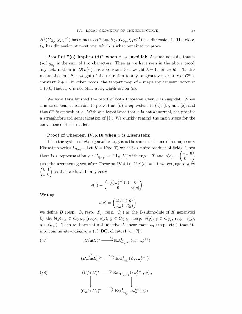
IV.6. LOCAL GEOMETRY OF THE EIGENCURVE 167
H1(GQp , χ2χ−11 ) has dimension 2 but H1
/f (GQp , χ2χ−11 ) has dimension 1. Therefore,
tD has dimension at most one, which is what remained to prove.
Proof of ”(a) implies (d)” when x is cuspidal: Assume non-(d), that is
(ρx)|GQpis the sum of two characters. Then as we have seen in the above proof,
any deformation in D(L[ε]) has a constant Sen weight k + 1. Since R = T, this
means that one Sen weight of the restrction to any tangeant vector at x of C± is
constant k + 1. In other words, the tangent map of κ maps any tangent vector at
x to 0, that is, κ is not etale at x, which is non-(a).
We have thus finished the proof of both theorems when x is cuspidal. When
x is Eisenstein, it remains to prove that (d) is equivalent to (a), (b), and (c), and
that C± is smooth at x. With our hypotheses that x is not abnormal, the proof is
a straightforward generalization of [?]. We quickly remind the main steps for the
convenience of the reader.
Proof of Theorem IV.6.10 when x is Eisenstein:
Then the system of H0-eigenvalues λx,0 is is the same as the one of a unique new
Eisenstein series E2,ψ,τ . Let K = Frac(T) which is a finite product of fields. Then
there is a representation ρ : GQNp → GL2(K) with tr ρ = T and ρ(c) =
Ç−1 00 1
å(use the argument given after Theorem IV.4.1). If ψ(c) = −1 we conjugate ρ byÇ
0 11 0
åso that we have in any case:
ρ(c) =
Çτ(c)ωk+1
p (c) 00 ψ(c)
å.
Writing
ρ(g) =
Ça(g) b(g)c(g) d(g)
åwe define B (resp. C, resp. Bp, resp. Cp) as the T-submodule of K generated
by the b(g), g ∈ GQ,Np (resp. c(g), g ∈ GQ,Np, resp. b(g), g ∈ GQp , resp. c(g),
g ∈ GQp). Then we have natural injective L-linear maps ιB (resp. etc.) that fits
into commutative diagrams (cf [BC, chapter1] or [?]):
(B/mB)∗
ιB// Ext1GQ,Np(ψ, τω
k+1p )
(Bp/mBp)
∗ιBp // Ext1
GQp(ψ, τωk+1
p )
(87)
(C/mC)∗
ιC// Ext1GQ,Np(τω
k+1p , ψ)
(Cp/mCp)
∗ιCp // Ext1
GQp(τωk+1
p , ψ)
,(88)
168 IV. THE EIGENCURVE OF MODULAR SYMBOLS
where the left vertical maps are dual of the inclusion Bp ⊂ B and Cp ⊂ C, and
the top vertical maps are restriction maps. Moreover, by Kisin’s lemma the imagoe
of ιB lies in the subspace of Ext1GQ,Np(ψ, τω
k+1p ) paremetrizing extensions that are
crystalline at p. As seen is the proof of Lemma IV.6.6, this subspace has dimension
1. It follows that B/mB has dimension at most 1, and by Nakayama that B is a
principal ideal. Also, from the proof of Lemma IV.6.6 we get that the restriction
map Ext1GQ,Np(τω
k+1p , ψ)→ Ext1
GQp(τωk+1
p , ψ) is an isomorphism between spaces of
dimension 1 and we conclude as above that C and Cp are principal, and even that
they are equal provided that Cp 6= 0.
The ideal BC (resp. BpCp) is the reducibility ideal of T (resp. T|GQp) as defined
in [BC, chapter 1] or [?]. It is proved in [?] that BpCp is the ideal of the schematic
fiber of κ at k and that BC is the maximal ideal m of T. By the above m is
principal, which shows that T is a discrete valuation ring, hence Theorem IV.6.10
in the Eisenstein case.
Equivalence between (a) and (d) in the Eisenstein case: We keep the
notations of the above paragraph. Since BC = m and BpCp is the ideal of the
fiber of κ, we see that (a) is equivalent to BpCp = BC. By what we have seen,
Cp = C (C being clearly non-zero since BC = m), so the later is equivalent to
Bp = B. By the commutative diagram (87) this is equivalent to restriction map
Ext1GQ,Np(ψ, τω
k+1p ) → Ext1
GQp(ψ, τωk+1
p ) being injective, which by construction of
ρPx is clearly equivalent to (d).
There are two noteworthy abnormal cases where the same (and actually even
stronger) results hold, with some modification of the proof:
Theorem IV.6.12. Assume that x is a very classical point of weight κ(x) = 0, of
critical slope vp(Up(x)) = 1, and such that the system of eigenvalues of x restricted
to H0, λx,0 : H0 → L is either the system of Eigenvalues of E2 or the system of
eigenvalues of E2,τ,τ where τ is a non-trivial Dirichlet character (note that such
very classical points x exist on C± if and only if ± = +1). Then the weight map κ
is etale at x, and in particular
conclusions of Lemma IV.6.6, TheoremIV.6.10, and Theorem IV.6.9, hold.
Moreover, the condition (a) to (d) of Theorem IV.6.9 are true.
Proposition IV.6.13. Assume that the tame level is a prime power N = lν , and
that x is a very classical point of weight κ(x) = 0, of critical slope vp(Up(x)) = 1.
Assume that the system of eigenvalues of x restricted to H0, λx,0 : H0 → L is
either the system of Eigenvalues of E2,l or the system of eigenvalues of E2,τ,τ where
τ is a primitive non-trivial Dirichlet character, necessarily of conductor a power
of l. (Note that such very classical points x exists on C± if and only if ± = +1).
Then the conclusions of Lemma IV.6.6, TheoremIV.6.10, and Theorem IV.6.9,
hold. Moreover, the condition (a) to (d) id Theorem IV.6.9 are true.

IV.7. NOTES AND REFERENCES 169
Proof — In the proof of Lemma IV.6.6, the only thing that changes is the proof
that the space (86) has dimension 1. Namely, we now have to prove that
kerÄH1(GQ,Np, ωp)→ H1
/f (GQp , ωp)ä
is of dimension 1. By Kummer theory, this dimension of this space is the rank of
the group of N -units in Q, so is 1 if (and only if) N is a prime power. For the
extensions in the other direction, nothing changes.
In the proof of the theorems, we see that nothing changes until the computation
of the rank of ιB, but the result is the same (that is 1) by the above paragrap. The
computation of the rank of ιC is not changed. Hence the theorems hold. Assertion
(d) of Theorem IV.6.9 hold since a N -unit of Q of infinite order obviously is also
of infinite order when seen in Qp.
Remark IV.6.14. For the other abnormal very classical critical-slope points,
Lemma IV.6.6 is false, as there are in this case several independent non-isomorphic
extension of ψ by τωp in the category of GQ,Np-representation that are crystalline
at p. I do not know if IV.6.10, and Theorem IV.6.9 hold in this case, but it is
unlikely. For example, if C± was smooth at x in this case, then Ribet’s lemma
would single out a canonical non-trivial extension of ψ by τωp as above, and I don’t
see why any of those extensions would deserve such a privilege.
IV.7. Notes and References

CHAPTER V
The two-variables p-adic L-function on the eigencurve
V.1. Abstract construction of an n+ 1-variables L-function
Let us place ourselves in the situation of the construction of the eigenalgebra:
H is a commutative ring, R is a commutative Noetherian ring, M a finite flat
R-module with an R-linear action of H, so the eigenalgebra T is defined as the
sub-algebra of EndR(M) generated by the action of H; the algebra T is finite flat
over R and M is naturally a finite T -module. To help the geometric intuition, let
us call X = Spec T , W = SpecR, and let denote by κ the structural map X →W .
If x is a closed point in X corresponding to a maximal ideal px of T , then w := κ(x)
is a closed point of W , corresponding to the maximal ideal pw = px ∩R of R. Let
L(x) = T /px and L(w) = R/pw be the field of definition of x and w, so that L(x)
contains L(w) and is of dinite degree over it. Let us call Mw the L(w)-vector space
with H-action M ⊗R,w L(w) = M/pwM , and Mw[x] the L(x)-vector space defined
as the eigenspace for H with tha same eigenvalue as x in Mw ⊗L(w) L(x).
We write M∨ = HomR(M,R) and provide it with its natural structure of T -
module (hence of H-module).
Lemma V.1.1. (i) We have a natural isomorphism of L(x)-vector space
M∨/pxM∨ '−→Mw[x]∨
(ii) Assume M∨ is free of rank one over T , and fix a generator u of M∨. Call
ux the image of u by the isomorphism (i). Then ux is a generator of the
one-dimensional L(x)-vector space Mw[x]∨.
Proof — Sine M is finite flat over R, we have a natural isomorphism M∨/pwM∨ =
(M/pwM)∨ = M∨w . Thus M∨/pxM∨ is the quotient of M∨/pwM
∨ = M∨w by the
sum of the images of the maps T − x(T ). Hence by elementary duality theory, it is
naturally isomorphic to the dual of the intersection of the kernel of these maps in
Mw ⊗L(w) L(x), that is to Mw[x]∨. This proves (i). If M∨ is free of rank one over
T , generated by u, then M∨/pxM∨ is of dimension 1 over L(x) and generated by
the image of u, and (ii) follows.
Now assume that R is a Qp-affinoid reduced algebra provided with the supre-
mum norm || ||sup, and that M is provided with some norm || || which takes values
in pZ ∪ 0and makes M a normed R-module. We provide Mw = M/pwM of the
quotient norm || ||w, which makes it a normed finite-dimensional L(w)-vector space
171

172 V. THE TWO-VARIABLES p-ADIC L-FUNCTION ON THE EIGENCURVE
where L(w) is provided with the unique norm that extends Qp. We provide L(x)
with its unique norm extending the norm of Qp, Mw ⊗L(w) L(x) with the tensor
norm, Mw[x] with the restriction || ||x of the latter norm, and finally Mw[x]∨ of the
dual norm, denoted || ||′x. By the theorem of Hahn-Banach, || ||′x is also the quotient
norm on Mw[x]∨ of the extension to L(x) of the norm || ||′w on M∨w which is dual of
|| ||w.
Lemma V.1.2. Assume that T is reduced, that M∨ is free of rank one over T ,
and that u is a generator of M∨. Then there exist two real numbers 0 < c < C
such that for every closed point of T , one has
c ≤ ||ux||′w ≤ C.
Proof — From the very nature of the result we want to prove, we can replace the
given norm on M by an equivalent one. Since M is free, choose an isomormorphism
M ' Rn and give M the norm that makes this isomorphism an isometry. This norm
is equivalent to the given one by [BGR, Prop. 3.7.3/3]. Choosing this norm || ||ensures that if we provide M∨ with the dual norm || ||′, then the norm || ||′w on M∨wis the quotient norm of || ||′. Therefore the norm || ||′x on M∨/pxM
∨ is also the
quotient norm of the norm || ||′ on M∨.
We thus are reduced to show that the norm of ux in M∨/pwM∨ lies between
two positive constants c and C, and again, it is enough to prove this after changing
the norm on M∨ by an equivalent one. Consider the T -isomorphism M∨ → Tthat sends u to 1. Provide T with its supremum norm (it is a norm because T is
reduced) and M∨ with the norm that makes this isomorphism an isometry. Now
our problem is just to show that for the supremum norm of T , the quotient norm
of the unity 1 in any quotient T/p is bounded between two positive constants. But
thoses quotients norms are always 1.
We keep the above hypothesis and suppose given, in addition, an R-linear map
h : M → D(R), where D(R) is the R-module of (families of) distributions (cf
§III.4.4). This map induces, for every finite extension of Qp and w ∈W (L), L-linear
maps hw : Mw → D(L) defined by hw = h⊗ 1 : Mw = M ⊗r,w L→ D(R)⊗R,w L =
D(L), the last equality being Cor. III.4.26 using that the completed tensor product
by L over R is the same as the usual tensor product. (In the application, elements
of M and Mw shall be distribution-valued modular symbol and h, or hw, shall be
eveluation at the divisor 0 − ∞)
Definition V.1.3. Assume that M∨ is free of rank one over T .
(i) For each closed point x of X, of field of definition L, a distribution µx ∈D(L), well-defined up to multiplication by an element of O∗L
(ii) A ”family of distributions” µ ∈ D(T ) well-defined up to a multiplication
by an element of T ∗.
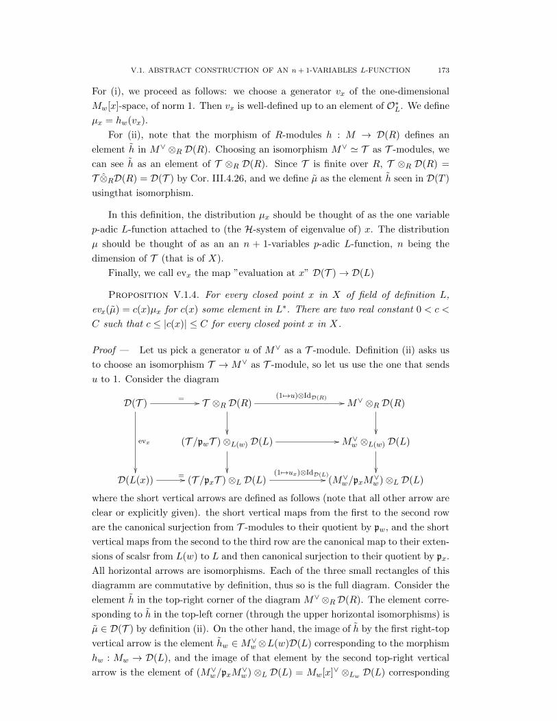
V.1. ABSTRACT CONSTRUCTION OF AN n+ 1-VARIABLES L-FUNCTION 173
For (i), we proceed as follows: we choose a generator vx of the one-dimensional
Mw[x]-space, of norm 1. Then vx is well-defined up to an element of O∗L. We define
µx = hw(vx).
For (ii), note that the morphism of R-modules h : M → D(R) defines an
element h in M∨ ⊗R D(R). Choosing an isomorphism M∨ ' T as T -modules, we
can see h as an element of T ⊗R D(R). Since T is finite over R, T ⊗R D(R) =
T ⊗RD(R) = D(T ) by Cor. III.4.26, and we define µ as the element h seen in D(T )
usingthat isomorphism.
In this definition, the distribution µx should be thought of as the one variable
p-adic L-function attached to (the H-system of eigenvalue of) x. The distribution
µ should be thought of as an an n + 1-variables p-adic L-function, n being the
dimension of T (that is of X).
Finally, we call evx the map ”evaluation at x” D(T )→ D(L)
Proposition V.1.4. For every closed point x in X of field of definition L,
evx(µ) = c(x)µx for c(x) some element in L∗. There are two real constant 0 < c <
C such that c ≤ |c(x)| ≤ C for every closed point x in X.
Proof — Let us pick a generator u of M∨ as a T -module. Definition (ii) asks us
to choose an isomorphism T →M∨ as T -module, so let us use the one that sends
u to 1. Consider the diagram
D(T )
evx
= // T ⊗R D(R)
(1 7→u)⊗IdD(R) // M∨ ⊗R D(R)
(T /pwT )⊗L(w) D(L)
// M∨w ⊗L(w) D(L)
D(L(x))
= // (T /pxT )⊗L D(L)(17→ux)⊗IdD(L)// (M∨w/pxM
∨w)⊗L D(L)
where the short vertical arrows are defined as follows (note that all other arrow are
clear or explicitly given). the short vertical maps from the first to the second row
are the canonical surjection from T -modules to their quotient by pw, and the short
vertical maps from the second to the third row are the canonical map to their exten-
sions of scalsr from L(w) to L and then canonical surjection to their quotient by px.
All horizontal arrows are isomorphisms. Each of the three small rectangles of this
diagramm are commutative by definition, thus so is the full diagram. Consider the
element h in the top-right corner of the diagram M∨⊗RD(R). The element corre-
sponding to h in the top-left corner (through the upper horizontal isomorphisms) is
µ ∈ D(T ) by definition (ii). On the other hand, the image of h by the first right-top
vertical arrow is the element hw ∈M∨w ⊗L(w)D(L) corresponding to the morphism
hw : Mw → D(L), and the image of that element by the second top-right vertical
arrow is the element of (M∨w/pxM∨w) ⊗L D(L) = Mw[x]∨ ⊗Lw D(L) corresponding

174 V. THE TWO-VARIABLES p-ADIC L-FUNCTION ON THE EIGENCURVE
to the restriction of hw to Mw[x]. The element in D(L) correspinding to that ele-
ment through the (through the lowwer horizontal isomorphisms) is clearly hw(u′x),
where u′x is the unique element of Mw[x] such that ux(u′x) = 1. For vx any gener-
ator of Mw[x] of norm 1, as in definition (i), we have u′x = c(x)vx with c(x) ∈ L∗
and |c(x)| = ||u′x||w = (||ux||′w)−1 is bounded between two positive constants by
Lemma V.1.2. By commutativity of the diagram, we thus have shown
evx(µ) = hw(u′x) = c(x)hw(vx) = c(x)µx
and the proposition is proven.
V.2. Good points on the eigencurve
Lemma V.2.1. Let x be a point on C± (of field of definition L), with κ(x) =
w ∈ W. The following statements are equivalent:
(i) The dual of generalized eigenspace Symb±Γ (Dw(L))∨(x) is free of rank 1 over
the algebra Tx of the schematic fiber of κ at x.
(ii) For any clean neighborhood of x, the module M∨ is flat of rank one over
T at x (we use the notations of §IV.6.1).
(iii) For any sufficiently small clean neighborhood of x, the module M∨ is free
of rank one over T at x.
Proof — The equivalence between (ii) and (iii) is clear. If U is a clean neighbor-
hood, x is the only point of U above w, so Tx is the fiber Tw of T at w and the fiber
Mw of M at w is Symb±Γ (Dw)(x) (cf. §IV.6.1), hence Symb±Γ (Dw)∨(x) is the fiber of
M∨ at w. Since M∨ and T are finitie flat over R, Nakayama’s lemma implies that
(i) is equivalent to (ii).
Definition V.2.2. A point x ∈ C± satisfying the conditions of the above lemma
is called a good point.
If x is a good point, there exists a clean neighborhood of x where all points are
good (by (iii) of the Lemma).
Theorem V.2.3. If x is a good point of field of definition L, κ(x) = w, then
the eigenspace Symb±Γ (Dw(L))[x] has dimension 1
Proof — Let U = Sp T be a clean neighborhod as in (ii) of Lemma V.2.1. Since
T is the eigenalgebra of H acting on M , it is aso the eigenalgebra of H acting on
M∨ (cf. exercise I.3.4). Hence since M∨ is flat over T , by Prop. I.4.3 the fiber Twis the eigenalgebra of H acting on (M∨)w = M∨w . Thus Tw = Tx is the eigenalgeba
of H acting on M∨w = Symb±Γ (Dw(L))∨(x).
On the other hand, since Symb±Γ (Dw(L))(x) is free of rank 1 over Tx, then
Symb±Γ (Dw(L))∨(x)/pxSymb±Γ (Dw(L))∨(x) where px is the maximal ideal of the local
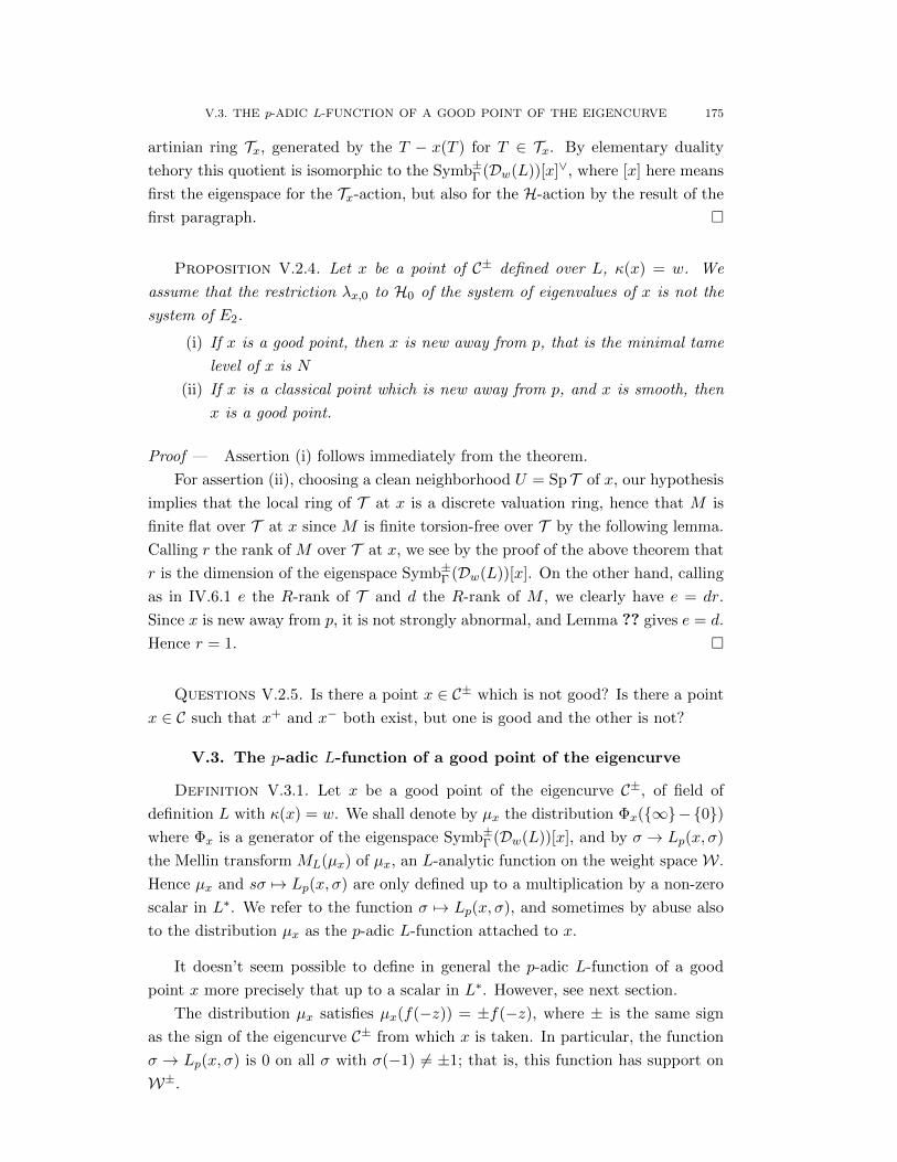
V.3. THE p-ADIC L-FUNCTION OF A GOOD POINT OF THE EIGENCURVE 175
artinian ring Tx, generated by the T − x(T ) for T ∈ Tx. By elementary duality
tehory this quotient is isomorphic to the Symb±Γ (Dw(L))[x]∨, where [x] here means
first the eigenspace for the Tx-action, but also for the H-action by the result of the
first paragraph.
Proposition V.2.4. Let x be a point of C± defined over L, κ(x) = w. We
assume that the restriction λx,0 to H0 of the system of eigenvalues of x is not the
system of E2.
(i) If x is a good point, then x is new away from p, that is the minimal tame
level of x is N
(ii) If x is a classical point which is new away from p, and x is smooth, then
x is a good point.
Proof — Assertion (i) follows immediately from the theorem.
For assertion (ii), choosing a clean neighborhood U = Sp T of x, our hypothesis
implies that the local ring of T at x is a discrete valuation ring, hence that M is
finite flat over T at x since M is finite torsion-free over T by the following lemma.
Calling r the rank of M over T at x, we see by the proof of the above theorem that
r is the dimension of the eigenspace Symb±Γ (Dw(L))[x]. On the other hand, calling
as in IV.6.1 e the R-rank of T and d the R-rank of M , we clearly have e = dr.
Since x is new away from p, it is not strongly abnormal, and Lemma ?? gives e = d.
Hence r = 1.
Questions V.2.5. Is there a point x ∈ C± which is not good? Is there a point
x ∈ C such that x+ and x− both exist, but one is good and the other is not?
V.3. The p-adic L-function of a good point of the eigencurve
Definition V.3.1. Let x be a good point of the eigencurve C±, of field of
definition L with κ(x) = w. We shall denote by µx the distribution Φx(∞−0)where Φx is a generator of the eigenspace Symb±Γ (Dw(L))[x], and by σ → Lp(x, σ)
the Mellin transform ML(µx) of µx, an L-analytic function on the weight space W.
Hence µx and sσ 7→ Lp(x, σ) are only defined up to a multiplication by a non-zero
scalar in L∗. We refer to the function σ 7→ Lp(x, σ), and sometimes by abuse also
to the distribution µx as the p-adic L-function attached to x.
It doesn’t seem possible to define in general the p-adic L-function of a good
point x more precisely that up to a scalar in L∗. However, see next section.
The distribution µx satisfies µx(f(−z)) = ±f(−z), where ± is the same sign
as the sign of the eigencurve C± from which x is taken. In particular, the function
σ → Lp(x, σ) is 0 on all σ with σ(−1) 6= ±1; that is, this function has support on
W±.
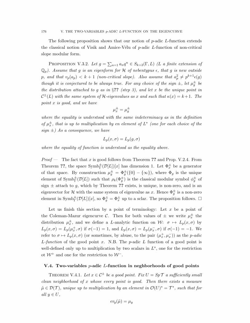
176 V. THE TWO-VARIABLES p-ADIC L-FUNCTION ON THE EIGENCURVE
The following proposition shows that our notion of p-adic L-function extends
the classical notion of Visik and Amice-Velu of p-adic L-function of non-critical
slope modular form.
Proposition V.3.2. Let g =∑n=1 anq
n ∈ Sk+2(Γ, L) (L a finite extension of
Qp). Assume that g is an eigenform for H of nebentypus ε, that g is new outside
p, and that vp(ap) < k + 1 (non-critical slope). Also assume that a2p 6= pk+1ε(g)
though it is conjectured to be always true. For any choice of the sign ±, let µ±g be
the distribution attached to g as in §?? (step 3), and let x be the unique point in
C±(L) with the same system of H-eigenvalues as x and such that κ(x) = k+1. The
point x is good, and we have
µ±x = µ±g
where the equality is understood with the same indeterminacy as in the definition
of µ±x , that is up to multiplication by en element of L∗ (one for each choice of the
sign ±) As a consequence, we have
Lp(x, σ) = Lp(g, σ)
where the equality of function is understood as the equality above.
Proof — The fact that x is good follows from Theorem ?? and Prop. V.2.4. From
Theorem ??, the space Symb±Γ (D[L])[x] has dimension 1. Let Φ±x be a generator
of that space. By consutruction µ±g = Φ±g (0 − ∞), where Φg is the unique
element of Symb±Γ (D[L]) such that ρk(Φ±g ) is the classical modular symbol φ±g of
sign ± attach to g, which by Theorem ?? exists, is unique, is non-zero, and is an
eigenvector for H with the same system of eigenvalue as x. Hence Φ±g is a non-zero
element in Symb±Γ (D[L])[x], so Φ±g = Φ±x up to a sclar. The proposition follows.
Let us finish this section by a point of terminology: Let x be a point of
the Coleman-Mazur eigencurve C. Then for both values of ± we write µ±x the
distribution µ±x , and we define a L-analytic function on W: σ 7→ Lp(x, σ) by
Lp(x, σ) = Lp(µ+x , σ) if σ(−1) = 1, and Lp(x, σ) = Lp(µ
−x , σ) if σ(−1) = −1. We
refer to σ 7→ Lp(x, σ) (or sometimes, by abuse, to the pair (µ+x , µ
−x )) as the p-adic
L-function of the good point x. N.B. The p-adic L function of a good point is
well-defined only up to multiplication by two scalars in L∗, one for the restriction
ot W+ and one for the restriction to W−.
V.4. Two-variables p-adic L-function in neghborhoods of good points
Theorem V.4.1. Let x ∈ C± be a good point. Fix U = Sp T a sufficiently small
clean neighborhood of x whose every point is good. Then there exists a measure
µ ∈ D(T ), unique up to multiplication by an element in O(U)∗ = T ∗, such that for
all y ∈ U ,
evy(µ) = µy

V.4. TWO-VARIABLES p-ADIC L-FUNCTION IN NEGHBORHOODS OF GOOD POINTS 177
where µy is the distribution attached to y as in Definition ??, well-defined up to an
element of L∗, and the equality is up to that indeterminacy.
Moreover, a choice of µ as above being fixed, there exists two constants 0 <
c < C such that if y is a point of U with κ(y) = k ∈ Z with the same system of
eigenvalues as a cusipidal eigenform g ∈ Sk+2(Γ, L), then we have evy(µ) = c(y)µ±gwhere c(y) is an element of L∗ so that c < |c(y)| < C.
Proof — Since x is good, choosing the clean neighborhood U small enough ensures
that M is free of rank one over T . We recall that M = εSymbΓ(DK(R))≤ν for
some real ν, and some idempotent ε. Let us fix a positive real r such that r <
r(K). Then SymbΓ(DK(R))≤ν = SymbΓ(DK [r](R))≤ν and thus we can provide
SymbΓ(DK(R))≤ν with the norm || ||r. We provide M with the restriction of that
norm.
We are now in posiition to apply the formalism of section V.1. For w ∈W , we
have Mw = εSymb±Γ (DK [r](L))≤νg and the quotient norm of the norm || ||r is still
the norm || ||r by ...
We define an R-linear map h : M → D(R) as h(Φ) = Φ(∞ − 0). Then
clearly the maps hw : Mw = εSymb±Γ (Dw(L))≤ν → D(L) defined from h as in §??
are also the evaluation at ∞ − 0.Definition V.1 gives us a distribution µ ∈ D(T ), and for every y ∈ U(L) with
κ(y) = w a distribution µy ∈ D(L), defined as hw(vy) where vy is a generator
of Mw[y] such that ||vy||r = 1. This definition of µy (up to an element of O∗L) is
obviously compatible with the definition (which is less precise: up to an element of
L∗) hence the first part of the theorem follows from the first part of Prop. V.1.4.
For the second part, let us assume that y corresponds to an eingenform g as
in the statement of the theorem. Then we need to compare µy = hw(vy) with
µ±g = φg(Φ±g ), where Φ±g is defined (up to O∗L) as an element of Symb±Γ (Dk(L))[g]
which satisfies ρ∗k(Φ±g ) is a generator of Symb±Γ (Vk(OL))[g], in other words such
that ||ρ∗k(Φ±g )|| = 1. Since ρk is an isometry for || ||1 on Symb±Γ (Dk(L))≤k+1, the
later condition of equivalent to ||Φ±g ||1 = 1. By Prop. III.6.27, there exists therefore
some constant D > 0 depending of our clean neighbrohood U and of the choice of
r, but independent of the choice of the classical point y or of the corresponding
modualr form g such that
D ≤ ||φ±g ||r ≤ 1.
Writing vy = c′(y)Φ±g with c′(y) ∈ L∗, we see that 1 ≤ |c′(y)| ≤ D−1 since by
defintion ||vy||r = 1. Since µy = c′(y)µ±g and evy(µ) = c(y)µy = c(y)c′(y)µ±g with
c(y) bounded between two positive constants by Prop. V.1.4, the theorem follows.
Corollary V.4.2. With U as in the above theorem, there exist a two-variable
analytic function L on U ×W, well-defined up to an element of O(U)∗, such that

178 V. THE TWO-VARIABLES p-ADIC L-FUNCTION ON THE EIGENCURVE
for all y ∈ U , and all σ ∈ W
L(y, σ) = L(y, σ)
where the equality is up to a scalar in L∗. Moreover, there exist two constant
0 < c < C such that if y corresponds to a modular eigenform g of non-critical
slope, we have
L(y, σ) = c(y)L(g, σ)
with c ≤ |c(y)| ≤ C.
V.5. Notes and References
CHAPTER VI
Adjoint p-adic L-function and the ramification locus ofthe eigencurve
This chapter is largely inspired by Kim’s 2006 Berkeley thesis [K]. Indeed the
core result, namely the construction of a scalar product on the module of families
of modular symbols interpolating the classical scalar product on classical modular
symbols is taken directly from [K], with only minor modifications. However, we
improve on Kim’s treatment by proving an explicit and more general result of
perfectness on this scalar product (such a result is implicitly stated in [K, Theorem
11.2]), and more importantly by changing the way the adjoint p-adic L-function
is constructed from the scalar product, and the way this scalar product is proved
to be related to the ramification locus of the eigencurve. Actually, we propose a
conceptual treatment of those two aspects together in subsection VI.1 below. It
seems to us that there is an gap in the argument of [K] concerning the descent of
the adjoint p-adic L-function to the eigencurve from its normalization) that our
method allows to circumvent. At any rate, we obtain more precise results on the
relation between the geometry of the weight map and the adjoint p-adic L-function.
Let us now describe in more details these results. As usual, we denote by
C0 the cuspidal eigencurve on tame level N . We construct, using Kim’s scalar
product on modular symbols, a canonical sheaf of ideals Ladj of O(C0), and we prove
(Theorem VI.4.2) that its closed locus contains all points of C0 where the weight
map κ is not etale. We ignore if the iseal Ladj is everywhere locally principal, but
it is so in a neighborhood of most points of interest, including all classical points
that are of minimal tame level N (except possibly for a few Eisenstein series of
weight 2 when N is not square-free) and all their companion points when they have
one. In a suitable neighborhood U of such a good point, we can define the p-adic
adjoint LadjU as a generator of the ideal Ladj, and we can determine exactly where
this function vanishes (see Theorem VI.4.7):
(i) If x ∈ U is a point that either has non-integral weight κ(x) 6∈ N, or is
cuspidal classical, then LadjU (x) = 0 if and only if teh weight map κ is etale
at x.
(ii) Otehrwise, that is if x ∈ U has κ(x) = k ∈ N and x is not a cuspidal
classical point (such points x are necessarily slope ≥ k+1), then LadjU (x) =
0 anyway.
179

180VI. ADJOINT p-ADIC L-FUNCTION AND THE RAMIFICATION LOCUS OF THE EIGENCURVE
Note that in case (ii) it may or may not happen that κ is etale at x. For example,
if x corresponds to an evil Eisenstein series of minimal tame level N , then it is
expected that κ is etale at x, and this is known for example for the Eisenstein
series Ecritk (for any even k > 4, so for N = 1) when p is a regular prime. On
the other hand, if x corresponds to the Eisenstein series Ecrit2,` (where ` 6= p is an
auxiliary prime,and E2,`(z) = E(z) − `E2(`z), and Ecrit2,` is the criticial refinement
at p of Ecrit2,` ) of an eigencurve of tame level N where N is divisible by at least two
primes, then it is not hard to prove (see a work of D. Majumdar for details) that
several components of the eigencurve C0 meet at x, and therefore that κ is not etale
at x.
When x is a smooth point of the eigencurve (again this includes almost all
classical points), we can define two invariants at x: the degree of ramification e(x)
of κ at x (so κ is etale at x if and only if e(x) = 1), and the order of vanishing of
LadjU at x. It is natural to ask how these invariants are related : an answer is given
in Theorem VI.4.8.
Finally we need to justify the name of the adjoint p-adic L-function LadjU by
proving that at cuspdial classical point of non-critical slope x corresponding to the
form fx, the value LadjU (x) is related to the value of the archimedean adjoint p-adic
L-function of fx at the near central point. Kim ([K, Theorem 12.3]) proves such
a formula in the case fx has wild level pr with r ≥ 1 and primitive nebemtypus.
We extend this formula to the case of a form of level p and trivial nebentypus,
in particular a form fx which is a refinement of a form of level prime to p (note
typsetted yet).
VI.1. The L-ideal of a scalar product
In all this §, R is a Noetherian domain (of fraction field K), and T is a finite
R-algebra.
VI.1.1. The Noether different of T/R. Let m : T ⊗R T → T denotes the
multiplication map: m(t⊗ u) = tu. Let I be the kernel of this map.
Lemma VI.1.1. As an ideal of T ⊗R T the ideal I is generated by the elements
of the form t⊗ 1− 1⊗ t for t ∈ T .
Proof — It is clear that t ⊗ 1 − 1 ⊗ t ∈ I. Conversely, if∑k tk ⊗ uk ∈ I then∑
tkuk = 0, hence∑k tk ⊗ uk =
∑(1⊗ uk)(tk ⊗ 1− 1⊗ tk) which shows the result.
A trivial but important remark is the following. If M is a T⊗RT -module, it has
two natural structures of T -modules, using the two natural morphisms of algebras
T → T ⊗R T : t 7→ t⊗ 1, t 7→ 1⊗ t. On the sub-module M [I] = m ∈M, Im = 0,the two T -structures coincide, and in fact, M [I] is the largest sub-module of M on
VI.1. THE L-IDEAL OF A SCALAR PRODUCT 181
which the two T -structures coincide. In particular, we can see M [I] as a T -module
unambiguously.
Definition VI.1.2 ([N]). The Noether’s different dN (T/R) is the ideal of T
which is the image of (T ⊗R T )[I] by m.
The Noether’s different is also called homological different.
The main interest of this notion is in the following theorem (due, it seems,
in this generality to Alexander-Buchsbaum). Recall that for any extension T/R
of algebras, a prime P of T is said unramified over R if for p = P ∩ R, we have
pTP = PTP, and TP/PTP is a finite separable extension of Rp/pRp. It is said
ramified if it is not unramified.
Theorem VI.1.3. A prime ideal P of S is ramified over R if and only if
dN (T/R) ⊂ P. In other words, the closed subset of SpecT defined by the Noether’s
different is the ramification locus of SpecT → SpecR.
For the proof, see [AB, Theorem 2.7]. Their theorem is even more general, as
they do not actually assume that T/R is finite, but the much weaker assumption
that T is Noetherian and I is finitely generated. We shall apply this result in a
situation where T/R is not only finite but also flat. In this case, P is unramified
over R if and only if it is etale, and if and only if it is smooth. Hence the closed
set of SpecT defined by the Noether’s different is also the set of points where
SpecT → SpecR is not etale.
There are at least two others notions of different. We shall not need them, but
for the sake of completeness, let us recall them quickly:
The oldest notion is Dedekind’s different which is defined only under supple-
mentary hypotheses. Namely one assumes that T is reduced, and calling K the
fraction ring of R and L the total fraction ring of T (which is finite product of
fields Li, each of them finite over K), we assume that L is etale over K (that
is, each of the Li is a separable extension of K). In Dedekind’s definition as in
most treatments of this notion in the literature, it is moreover assumed that R is
Dedekind, but this is not actually necessary. Here is how the Dedekind different
is defined: the trace map tr L/K defines a non-degenerate K-bilinear pairing on L:
(x, y) 7→ tr (xy). Let T ∗ be the set of x ∈ L such that tr L/K(xy) ∈ R for all y in T .
It is clear that T ∗ is a T -module, and that it is actually the largest T -submodule of
L such that tr L/K(T ∗) ⊂ R. In particular, since tr L/K(T ) = R, we have T ⊂ T ∗.
The Dedekind’s different dD(T/R) is the ideal [T : T ∗] of T , that is the set of
y ∈ T such that xT ∗ ⊂ T . This definition is the one given in all textbooks on
algebraic number theory (where R is invariably assumed to be Dedekind). See e.g.
[S, Chapter III] for a fairly complete treatment in this case.
The most modern notion is Kahler’s different dK(T/R) which is defined as
the 0-th fitting ideal of the module of differential forms ΩT/R (cf. [Ka]). More

182VI. ADJOINT p-ADIC L-FUNCTION AND THE RAMIFICATION LOCUS OF THE EIGENCURVE
concretely, we can compute Kahler’s different as follows: choose x1, . . . , xn a family
of generators of T as R-algebra, and let (P1, . . . , Pm) in R[X1, . . . , Xn] the ideals of
their algebraic relations over R. In other words R[X1, . . . , Xn]/(P1, . . . , Pm) ' T ,
the map sending Xi to xi. Note that we have m ≥ n since T is finite over R by
assumption but that it is not always possible to choose m = n (when it is, T is
said to be complete intersection over R). Form the m×n-Jacobian matrix in R[X]
whose (i, j) coefficients is ∂Pi∂Xj
. The Kahler’s different is then the T -ideal generated
by the image in T of the (n× n)-minors of that matrix. This is very easy from the
definitions of the module of differentials and of the Fitting ideal, both given in [E].
Recall that we always assume that R is a noetherian domain of fraction field K,
and that T/R is finite. The following result summarizes the known (to the author)
relations between those three notions.
Theorem VI.1.4. When T/R is flat, the ideal dN (T/R) and dK(T/R) define
the same closed subset of SpecT (that is, have the same radical), namely the set of
points where SpecT → SpecR is non-etale. The same is true if instead of assuming
that T/R is flat, we assume that R is integrally closed, that T is reduced, and that
the total fraction ring L of T is etale over K.
If T/R is flat and the Dedekind’s different is defined, it is equal to Noether’s
different dD(T/R) = dN (T/R).
If T/R is flat and locally complete intersection, then dN (T/R) = dK(T/R).
Proof — Since the 0-th Fitting ideal of a module defines the same closed subset
as the annihilator of that module, the closed set defined by the Kahler’s different is
the support of ΩT/R which is by definition the non-etale locus of SpecT → SpecR.
When T/R is finite and flat, the non-etale locus is the same as the ramification
locus of SpecT → SpecR since etale = flat and unramifed. The non-etale locus is
also the same as the ramification locus in the case we assume that R is integrally
closed that the total fraction ring of T is a product of finite separable extensions of(R), for in this case, an unramified point of SpecT is flat over SpecR by [AB, §4].
This completes the proof of the first paragraph of the theorem.
For the second assertion, see [N] or [AB, §3] (which contain more results along
this lines)
For the third assertion, see e.g. [Ku, Theorem 8.15].
VI.1.2. Duality. If M is a T -module which is finite and flat as an R-module,
the module M∨ := HomR(M,R) is also finite and flat over R, and has also a
T -module structure. Moreover we have a canonical isomorphism (M∨)∨ = M
as R-modules and even as T -modules, and for N a second T -module which is
finite and flat as an R-module the transposition defines a canonical isomorhism
HomT (M,N) = HomT (N∨,M∨).
VI.1. THE L-IDEAL OF A SCALAR PRODUCT 183
Note that the formation of HomR(M,N) and in particular of the T -module
M∨ commutes with any base change R → R′ in the obvious sense (This is proved
exactly as the special case M = N in §I.1.) The formation of HomT (M,N) however
only commutes in general with localizations of R.
If T is finite and flat over R, then the preceding apply to M = T and we can
define the T -module T∨, whose formation commutes with arbitrary base change.
We say that the R-algebra T is Gorenstein if T∨ is flat of rank one over T . Locally,
this is same as assuming the existence of an isomorphism of T -modules T∨ ' T .
Proposition VI.1.5. The natural isomorphism HomR(M,N) = M∨ ⊗R N
restricts to an isomorphism HomT (M,N) = (M∨ ⊗R N)[I].
Proof — Recall that the natural isomorphism is the one that sends∑i li ⊗ ni ∈
M∨ ⊗R N to the morphism f : M → N defined by f(m) =∑i li(m)ni (one checks
locally that it is an isomorphism). It is sufficient to observe then that∑i li ⊗ ni is
in (M∨ ⊗R N)[I] if and only if∑i(tli)⊗ ni =
∑i(li ⊗ tni) for all t ∈ T , if and only
if f is T -equivariant.
Corollary VI.1.6. Assume that T/R is flat. The R-algebra T is Gorenstein
if and only if (T ⊗R T )[I] is flat of rank one as T -module.
Proof — We may assume that R is local, and we have to prove in the case that
T/R is Gorenstein if and only if (T ⊗R T )[I] is free of rank one as T -module.
We have (T ⊗R T )[I] = HomT (T∨, T ). So if T/R is Gorenstein, T∨ ' T
and (T ⊗R T )[I] ' HomT (T, T ) = T as T -modules. Conversely, if (T ⊗R T )[I] is
isomorphic to T , then let f ∈ HomT (T∨, T ) corresponding to a generator of that
module. Then for t ∈ T , tf = 0 implies that t = 0. Therefore for t ∈ T , tf(T ) = 0
implies that t = 0. Since T is finite over R, it has no proper ideal having this
property, and f is surjective. By equality of R-rank, f is an isomorphism.
Corollary VI.1.7. If T/R is Gorenstein, dN (T/R) is a locally principal ideal.
Proof — Indeed, locally, this ideal is generated by m(g) where g is a generator of
(T ⊗R T )[I]
VI.1.3. The L-ideal of a scalar product. Now let M and N be two T -
modules, which as R-modules are finite flat. Let b : M ×N → R be an R-bilinear
scalar product which is T -equivariant (that is b(tm, n) = b(m, tn) for t ∈ T , m ∈M ,
n ∈ N).
184VI. ADJOINT p-ADIC L-FUNCTION AND THE RAMIFICATION LOCUS OF THE EIGENCURVE
Definition VI.1.8. We call Lb the ideal of T defined by the following con-
struction: extend by linearity the R-linear scalar product b to a T -bilinear scalar
product bT : (M ⊗R T )× (N ⊗R T )→ T . Set
Lb = bT ((M ⊗R T )[I], (N ⊗ T )[I]) ⊂ T.
Some clarifications may help: (M ⊗R T ) and (N ⊗R T ) have two T -modules
structures, or what amounts to the same, a T ⊗R T -module structure. The first
T -structure is given by the action of T on M or N , the second by the action of T on
T . When we say that bT is T -bilinear, we are referring to the second T -structure.
We note that the formation of Lb commute with localizations on R. (In general,
it doesn’t commute with arbitrarty base change, but see below).
Proposition VI.1.9. We have
Lb ⊂ dN (T/R)
Proof — Consider the map B : M⊗RT⊗RN⊗RT → T , m⊗t⊗n⊗u 7→ tub(m,n).
This maps clearly factors through the quotient (M ⊗R T ) ⊗T (N ⊗R T ) → T and
induces bT on that quotient. Hence
Lb = B((M ⊗R T )[I]), (N ⊗R T )[I].
There is an other way to factorize B:
B : M ⊗R T ⊗R N ⊗R T → Tc→ (M ⊗R N)⊗R (T ⊗ T )
b⊗1→ (T ⊗ T )m→ T.
where the first map is just the isomorphism c given by commutativity of tensor
product.
We claim that (b⊗ 1) c sends (M ⊗R T )[I]⊗R (N ⊗R T )[I]) into (T ⊗R T )[I].
Indeed if x =∑kmk ⊗ tk ∈ (M ⊗R T )[I], and y =
∑l nl ⊗ ul ∈ (N ⊗R T )[I] then
z := (b⊗ 1)(c(x, y)) =∑k,l b(mk, nl)tk ⊗ ul and we compute, for t ∈ T
(1⊗ t)z =∑k,l
b(mk, nl)tk ⊗ (tul)
=∑k,l
b(mk, tnl)tk ⊗ ul (using that Iy = 0)
=∑k,l
b(tmk, nl)tk ⊗ ul (using the T -equivariance of b)
=∑k,l
b(mk, nl)(ttk)⊗ ul (using that Ix = 0)
= (t⊗ 1)z
Hence we see that Ib = B((M ⊗R T )[I]⊗R (N ⊗R T )[I])) ⊂ m((T ⊗R T )[I]) =
dN (T/R).
VI.1. THE L-IDEAL OF A SCALAR PRODUCT 185
Proposition VI.1.10. Assume that M ' N ' T∨ as T -modules. Then the
ideal Lb of T is principal.
More precisely, the scalar product b can be seen as a linear map b : T∨⊗RT∨ →R. By duality, this is the same as an element b in T ⊗R T . We have Lb = m(b)T .
Proof — We have (M ⊗ T )[I] ' (T∨ ⊗ T )[I] = HomT (T, T ) = T . Let g be
a generator of this module. Similarly, let h be a generator of (N ⊗ T )[I]. Then
bT (g, h) is a generator of Lb.
For the ”more precisely”, let us identify M and N with T∨. Let ei be a basis of
T over R and e∨i a basis of T∨ over R. Take g = h =∑i e∨i ⊗ ei; it is a generator of
(T∨⊗T )[I], since it corresponds to the identity in HomR(T, T ). Then by definition:
bT (g, h) =∑i,j b(e
∨i , e∨j )eiejb(e
∨i , e∨j ). On the other hand, as an element of T ⊗R T ,
b is by definition∑i,j b(e
∨i , e∨j )ei ⊗ ej . Hence m(b) = bT (g, h) is a generator of Lb.
Corollary VI.1.11. Keep the assumptions of the preceding proposition. Then
the formation of Lb commutes with arbitrary base changes. (For the sake of pre-
cision, this means the following: if R′ is an R-algebra, let M ′ = M ⊗R R′, N ′ =
N ⊗R R′ and T ′ = R ⊗R R′. Let b′ : M ′ ⊗N ′ → R′ be the R′-bilinear extension of
b, which is clearly T ′-equivariant. Then the ideal Lb′ of T ′ is the ideal generated by
the image of Lb by the morphism T → T ′)
Proof — The assumption M ' N ' T∨ as T -modules implies similar assertions
over R′: M ′ ' N ′ ' T ′∨ as T ′-modules. The element b′ in T ′ ⊗R′ T ′ is just the
natural image of b, and thus Lb′ , which is the ideal generated by m(b′) is generated
by the image of m(b). The result follows.
Corollary VI.1.12. Assume that T/R is Gorenstein, and that M and N are
flat of rank one over T . Then Lb and dN (T/R) are locally principal, and Lb =
dN (T/R) if and only if b is non-degenerate. More precisely, if b = tb0 where b0 :
M×N → R is a non-degenerate T -equivariant scalar product, then Lb = tdN (T/R).
Proof — Note that since T/R is Gorenstein, locally T∨ ' T as T -module, so
we have M ' N ' T∨ and we are in a special case of the above proposition.
In particular, Lb is principal (locally), and we already know that the Noether’s
different is principal (locally) since T/R is Gorenstein.
For the rest of the proof we assume that R is local.
Clearly b is non-degenerate if and only if for all t ∈ T , tb = 0 implies t = 0, which
is equivalent to the same assertion for b. Since T is Gorenstein, (T ⊗ T )[I] = T ,
and we see that b is non-degnerate if and only if b is a generator of (T ⊗ T )[I].

186VI. ADJOINT p-ADIC L-FUNCTION AND THE RAMIFICATION LOCUS OF THE EIGENCURVE
Writing b = tb0 with t ∈ T , and where b0 is a generator of (T ⊗ T )[I], we have
m(b) = tm(b0) hence Lb = tdN (T/R) with equality if and only if t is invertible, i.e.
if and only if b is non-degenerate.
Remark VI.1.13. Let us go back to the hypothesis of Prop VI.1.3: M∨ and
N∨ free of rank one over T . If b is non-degenerate, then b defines an isomorphism
M ' N∨ as T -modules, so T∨ ' T and T is Gorenstein, and the corollary implies
that Lb = dN (T/R). Conversely, if Lb = dN (T/R), is it necessarily true that b is
non-degenerate (and therefore T Gorenstein)? I’d like to know the answer.
VI.2. Kim’s scalar product
Let us use the same notations of §IV.1: W = SpR is an open affinoid subset
of W, which belongs to the covering C (in particular R and its residue rong R
are PID, and N ∩ W is very Zarsiki-dense in W ), K : Z∗p → R∗ the canonical
character, and ν ≥ 0 is a real number, adapted to W . Let us fix a real r such that
0 < r < max(r(W ), p).
The aim of this section is to construct, if possible, an R-bilinear scalar prod-
uct b on SymbΓ(DK [r](R))≤ν that interpolate the corrected scalar products on
SymbΓ(Vk[r](Qp))≤ν , for k ∈ N ∩W (Qp) that we denoted by [ , ] (def. III.2.25),
corrected from the classical pairing defined using Poincares duality, cf. (28), Let us
precise what we mean by ”interpolate”. For any κ ∈W (L), where L is a finite ex-
tension of Qp, by extension of scalars κ : R→ L the scalar product b gives rises to a
L-bilinear scalar product bκ on SymbΓ(Dκ[r](R))≤ν⊗R,κL = SymbΓ(Dκ[r](L))≤νg ⊂SymbΓ(Dκ[r](L))≤ν (cf. Theorem IV.1.17 and the definition following it). If κ is
character z 7→ zk, and k ∈ N, SymbΓ(Dκ[r](Qp))≤ν admits the space of classical
modular symbols SymbΓ(Vk(Qp))≤ν as a quotient. By ”interpolating”, we mean
that the scalar product bk factors through that quotient and is equal, on that
quotient, to our old good corrected scalar product.
VI.2.1. A bilinear product on the space of overconvergent modular
symbols of weight k. Let k ≥ 0 be an integer. Assume that L is a finite extension
Qp. Remember the surjective map ρk : Dk[1](L)→ Vk(L), defined as the dual of the
inclusion Pk(L) → Ak[1](L) that we shall here denote by ik. Those maps ρk and
ik induce maps on modular symbols, e.g. ρk : SymbΓ(Dk[1](L))→ SymbΓ(Vk(L)).
Definition VI.2.1. We define a scalar product on SymbΓ(Dk[1](L)), denoted
by [ , ]k by
[Φ1,Φ2]k = [ρk(Φ1), ρk(Φ2)],
where [ , ] is the corrected scalar product on classical modular symbols, defined in
Def. III.2.25. We use the same notation [ , ]k for the restriction of this scalar prod-
uct to the finite-dimensional subspace SymbΓ(Dk[1](L))≤ν = SymbΓ(Dk[r](L))≤ν
(where r is any real number such that 0 < r < p).

VI.2. KIM’S SCALAR PRODUCT 187
We shall now give an explicit description of this scalar product. Below, we
consider Pk(L) with its right action of S, so that it is the contragredient of the
right S-module Vk(L). We denote by δ the tautological product Pk(L)×Vk(L)→ L.
Similarly we shall consider Ak[r](L) with its natural right action of S0(p)′ = γ ∈S, p|c, p 6 |d:
f|kγ(z) = (γ′ ·k f)(z) = (cz + d)kf
Åaz + b
cz + d
ãThe inclusion ik : Pk(L) → Ak[r](L) evidently respects our right action. We have
a natural pairing ∆ : Dk[r](L)×Ak[r](L)→ L defined by ∆(µ, f) = µ(f), which is
obviously compatible with δ in the sense that
∆(µ, ik(P )) = δ(ρk(µ), P ).(89)
We see by an easy computation
∆(µ|kγ , f|kγ) = det(γ)k∆(µ, f)
for all γ ∈ S0(p) ∩ S′0(p), and a similar formula holds for δ. In particular, the
pairings ∆ and δ are pairings of Γ0(p)-modules to L, so they define pairings, also
denoted ∆ and δ
∆ : SymbΓ(Dk[r](L))× SymbΓ(Ak[r](L))→ L,
δ : SymbΓ(Vk(L))× SymbΓ(Pk(L))→ L,
We now can compute:
[Φ1,Φ2]k = [ρk(Φ1), ρk(Φ2)] (by def. VI.2.1)
= (ρk(Φ1), ρk(Φ2)|WNp) (by def. III.2.25)
= δ(ρk(Φ1), θk(ρk(Φ2)|WNp))) (by def. 28)
= ∆(Φ1, ikθk(ρk(Φ2)|WNp) by (89)
= ∆(Φ1, Vk(Φ2)),
where Vk is the map
Vk : SymbΓ(Dk[r](L)) → SymbΓ(Ak[r](L))
Φ 7→ ikθk(ρk(Φ)|WNp).
Now Vk is easily described using the definitions of its constituents: for any D ∈∆0, ρk(Φ)(D)(zi) = Φ(D)(zi) provided that 0 ≤ i ≤ k. Then ρk(Φ)|WNp
(D)(zi) =
Φ(WNp ·D)(zi|kWNp) = Φ(WNp ·D)((−Npz)k−i). In other words,
ρk(Φ)|WNp(D) =
k∑i=0
Φ(W ·D)((−Npz)k−j)li,
where li ∈ Vk(L) is the linear form on Pk(L) sending zj to δi,j .

188VI. ADJOINT p-ADIC L-FUNCTION AND THE RAMIFICATION LOCUS OF THE EIGENCURVE
Using the formula for the operator θk given in Lemma III.2.1, we see that
θk(ρk(Φ)|WNp)(D)(z) =
k∑i=0
Φ(WNp ·D)((−Npz)k−i)(−1)iÇk
i
åzk−i
= (−1)kk∑i=0
(Np)iÇk
i
åΦ(WNp ·D)(zi) zi
Slightly more generally, we also have for any e ∈ Z
θk(ρk(Φ)|WNp)(D)(z) = (−1)k
k∑i=0
(Np)iÇk
i
åΦ(WNp ·D)(zi(1−Npez)k−i) (z − e)i
This follows by applying the above equality to Φ replaced by Φ|γ with γ =
Ç1 0
Npe 1
å∈
S, using that γ commutes with ρk and θk and that γWNp = WNp
Ç1 e0 1
å.
Applying ik amounts to seeing that polynomial in z as an element of A[r](L).
Such an element is described by its Taylor series about any e ∈ Zp, which is just
ιkθk(ρk(Φ)|WNp)(D)(z) = ((−1)k
k∑i=0
(Np)iÇk
i
åΦ(WNp ·D)(zi(1−Npez)k−i) (z−e)i
Note that in the above sum, we can replace∑ki=0 by
∑∞i=0 as the new terms are 0
because of their factor(ki
).
To summarize,
Proposition VI.2.2. For any Φ1,Φ2 ∈ SymbΓ(Dk[r](L)), we have
[Φ1,Φ2]k = ∆(Φ1, Vk(Φ2)),(90)
where Vk(Φ) ∈ SymbΓ(Ak[r](L)) is defined, for any D ∈ ∆0, e ∈ Zp, and z ∈ Zp,by
Vk(Φ)(D) = (−1)k∞∑i=0
(Np)iÇk
i
åΦ(WNp ·D)(zi(1−Npez)k−i) (z − e)i.(91)
VI.2.2. Interpolation of those scalar products. Let L be any Qp-Banach
algebra with a norm | | extending the p-adic norm of Qp, and κ ∈ W(L) be a
continuous character Z∗p → L∗.
Definition VI.2.3. (i) If y ∈ L, i ∈ N, we define(yi
)= y(y−1)...(y−i+1)
i! , if
i ≥ 0, and(y0
)= 1.
(ii) If κ ∈ W(L), we define(κi
)=(logp κ(γ)/ logp(γ)
i
), where γ is a generator of
1 + pZp
The first definition is standard and due to Isaac Newton. The second is easily
seen to be independent of the choice of γ, and to be compatible with the first one,
on the sense that(κi
)=(ki
)when κ is an integer k, that is to say the character
z 7→ zk,
Exercise VI.2.4. Prove that |(κi
)| < p
ipp−1

VI.2. KIM’S SCALAR PRODUCT 189
The key observation is that formula (91) makes sense when k is replaced by
an arbitrary character κ ∈ W(L). Indeed, for any Φ ∈ SymbΓ(Dk[r](L)), D ∈ ∆0,
e ∈ Zp, we can form the formal Taylor expansion at e:
Tκ,Φ,D,e(z) := κ(−1)∞∑i=0
(Np)iÇκ
i
åΦ(W ·D)(zi(1− eNz)k−i) (z − e)i.(92)
which when κ = k is exactly the RHS of (91).
Lemma VI.2.5. Assume that r < p−1p−1 . The series in the RHS of (92) converges
on the closed ball |z − e| < r.
Proof — We have |(Np)i| = p−i since N is prime to p,( |κ
i|<pipp−1
)by Exercise VI.2.4,
and |Φ(WNp · D)(zi(1 − eNz)k−i) ≤ ||Φ(WNp · D)||r since ||zi(1 − eNz)k−i||r ≤supz∈OCp
|zi(1 − eNz)k−i| ≤ 1. Hence the coefficient of (z − e)i has norm at most
pi
p−1 , which means that the series converges on disc any disc |z − e| < p−1p−1 , hence
the lemma.
Proposition VI.2.6. Let L be an affinoid algebra, κ ∈ W(L). We assume that
r < min(p−1p−1 , r(κ)).
(i) Fix Φ ∈ SymbΓ(Dκ[r](L)), and D ∈ ∆0. Then the convergent series
Tκ,Φ,D,e(z) for e ∈ Zp define an element in Ak[r](L).
(ii) Fix Φ ∈ SymbΓ(Dk[r](L)), and define Vκ(Φ) ∈ Hom(∆0,Ak[r](L)) by
sending D ∈ ∆0 to the element of Ak[r](L) defined in (i). Then Vκ(Φ) lies
in SymbΓ(Aκ[r](L))
Proof — This can probably be shown by brutal computation, but there is a more
clever way to do it.
We first consider a particular case: let us assume that L = R when SpR = W
is an affinoid of W belonging to C, and κ = K is the canonical character Z∗p → R∗.
To prove (i), we need to prove that for e, e′ in Zp, TK,φ,D,e(z) and TK,φ,D,e′(z) have
the same values for any z ∈ Zp such that |z − e| ≤ r, |z − e′| ≤ r. To prove that
those two elements of R are equal, it suffices to prove that there image by any
morphisms R→ Qp corresponding to an element k ∈ N∩W are equal, since N∩Wis Zariski-dense in W . But those images are just Tk,φ,D,e(z) and Tk,φ,D,e′(z), and
we know from the last paragraph that those two series actually define the same
polynomial independent of e, namely (−1)k∑ki=0(Np)i
(ki
)Φ(WNp ·D)(zi) zi. Hence
(i) is done in this case. For (ii), we need to prove that VK(Φ)|Kγ = VK(Φ) for γ ∈ Γ.
Again, this reduces to proving that Vk(Φ)|kγ = VK(Φ) for all integer k ∈ N ∩W ,
which we know since by definition Vk(Φ) ∈ SymbΓ(Dk[r]).The general case (L, κ) can be reduced to the the case (R,K) as follows. The
character κ ∈ W(L) defines a morphism SpL → W whose image is in some W =
SpR in C, since those W ’s form an admissible covering ofW. For such a W = SpR,

190VI. ADJOINT p-ADIC L-FUNCTION AND THE RAMIFICATION LOCUS OF THE EIGENCURVE
we have a morphism of algebra R→ L and the character κ is just the composition
of K with this morphism. Therefore, the case (L, κ) follows from (R,K) by base
change R → L (using that the formation of A[r](L) commute with arbitrary base
change, cf. Corollary III.4.15).
Definition VI.2.7. Let L be any Qp-affinoid algebra, κ ∈ W (L), and r <
min(p−1p−1 , r(κ)) We define a scalar product [ , ]κ on SymbΓ(Dk[r](L)) by the formula
[Φ1,Φ2]κ = ∆(Φ1, VκΦ2).
Theorem VI.2.8.
(i) The formation of this scalar product commutes with any affinoid base change
L 7→ L′, in the sense that if Φ1,Φ2 ∈ SymbΓ(Dk[r](L)), and Φ′1, Φ′2 are the image
of Φ1⊗1,Φ2⊗1 by the natural morphisms (which are not always isomorphisms!)
SymbΓ(Dk[r](L))⊗LL′ → SymbΓ(Dk[r](L′)), one has
[Φ′1,Φ′2] = [Φ1,Φ2]
(ii) When L = Qp, κ = k ∈ N, this scalar product coincides with the one denoted
[ , ]k above.
(iii) All the Hecke operators in H are self-adjoint for [ , ]κ.
Proof — (i) is clear since the ”Poincare duality” pairing ∆ is natural, and since
the formation of Vκ commute with base change by construction. (ii) is also clear
since Vκ = Vk when κ = k by construction. Finally (iii) is first proved for the case
(R,K) where W = SpR is an affinoid of W in C and K the canonical weight by
density from the case of integral weight (which is Lemma ??) and then for any
(L, κ) using (i).
Using SymbΓ(Dκ[r](L))≤ν is independent of r when it is defined (that is for ν
adpated to L and r < min(p, r(κ))), the above scalar product define by restriction
a scalar product on SymbΓ(Dκ[r](L))≤ν . We note also that by the formal property
of ∆, the scalar product [ , ]κ factors through the quotient H1! (Γ,Dk[r](L)).
Theorem VI.2.9. Let ν ≥ 0, and assume that L is a finite extension of Qp.
The restriction of [ , ]κ to H1! (Γ,Dk[r](L))≤ν is non-degenerate if κ 6∈ N or if
κ = k ∈ N and ν < k + 1.
Proof — Assume that Φ1 ∈ H1! (Γ,Dk[r](L))≤ν is such that [Φ1,Φ2]κ = 0 for all
Φ2 ∈ H1! (Γ,Dk[r](L))≤ν . Then since Up is self-adjoint, we have [Φ1,Φ2]κ = 0 for
all Φ2 ∈ H1! (Γ,Dk[r](L)). In view of the non-degeneracy of ∆, this means that
Vκ(Φ1) = 0. By the definition of Vκ, this means in particular that Tκ,Φ1,D,e(z) is 0
VI.3. GOOD POINTS ON THE CUSPIDAL EIGENCURVE 191
for every e ∈ Zp, D ∈ ∆0. Applying this to the divisor W−1Np ·D and to e = 0, we
get that for every D ∈ ∆0 and every integer i:Çκ
i
åΦ1(D)(zi) = 0.
In the case κ 6∈ N, then(κi
)is never 0. Therefore for all D ∈ ∆0, the distribution
Φ1(D) which belongs to D[1](L) satisfies Φ(D)(zi) = 0. Hence Φ1(D) = 0 and
Φ1 = 0.
In the case κ = k ∈ N, then at least(ki
)6= 0 for 0 ≤ i ≤ k and we have
Φ1(D)(zi) = 0
for all D ∈ ∆0 and 0 ≤ i ≤ k. This means that ρk(Φ1) = 0. If ν < k + 1, then this
implies again Φ1 = 0 by Stevens’ control theorem (Theorem III.6.36).
VI.3. Good points on the cuspidal eigencurve
We first need to define a notion of good point on the cuspidal eigencurve C0
analog to the one we defined on the eigencurves C± (cf. Definition ??). Recall that
the cuspidal eigencurve can be constructed by applying the eigenvariety machine
to three different eigenvariety data: to the modules of cuspidal overconvergent
forms, or to the modules of overconvergent modular symbols H1! (Γ,DK [r](R))±
for both values of the sign ±. That the three eigenvarieties obtanied these ways
are isomorphic (with unique isomorphisms respecting the Hecke operators and the
weight maps) was proved in Theorem ??. We shall use only the two definitions
with modular symbols. If x ∈ C(L), and U = Sp T is a clean neighborhood of x,
let as in §IV.6.1 W = SpR the image κ(U), and, for r > 0 sufficiently small, let
M± be the finite free R-module εH1! (DK [r](R))± (it is independent of r) where ε
is the idempotent corresponding to the connected component U of κ−1(W ).
The following lemma is proven exactly as Lemma V.2.1
Lemma VI.3.1. Let x be a point on C0 (of field of definition L), with κ(x) =
w ∈ W. The following statements are equivalent:
(i) For both choices of the sign ±, the dual of the generalized eigenspace
H1! (Dw(L))±(x) is free of rank 1 over the algebra Tx of the schematic fiber
of κ at x.
(ii) For both choices of the sign ±, and for any clean neighborhood of x, the
modules (M±)∨ are flat of rank one over T at x
(iii) For both choices of the sign ±, and for any sufficiently small clean neigh-
borhood of x, the modules (M±)∨ are free of rank one over T at x.
Definition VI.3.2. A point x ∈ C0 is called good if it satisfies the proposition
above.
192VI. ADJOINT p-ADIC L-FUNCTION AND THE RAMIFICATION LOCUS OF THE EIGENCURVE
Exactly as in Prop. V.2.4 and in the, we can prove that if x is a smooth point
of C0 which is classical and new away from p, then x is good.
We shall need the following lemma, which summarizes results obtained earlier:
Lemma VI.3.3. If x is a good point, then the eigenspace H1! (Dw(L))±[x] has di-
mension 1. If x is a good and of weight w(x) = k and H1! (Vk(L))±[x] has dimension
1 if x is very classical cuspidal, 0 otherwise, and the same is true for the generalized
eigenspaces H1! (Vk(L))±(x) provided Up(x)2 6= pk+1〈p〉(x). In the former case, the
map between one-dimensional spaces ρk : H1! (Dk(L))±[x] → H1
! (Vk(L))±[x] is an
isomorphism if κ is etale at x, and is 0 if κ is not. If x is a good point of weight
w(x) = k and vp(Up(x)) < k+1, then x is cuspidal and very classical and κ is etale
at x.
Proof — The first assertion follows by duality from the definition of a good point
(see Lemma VI.3.2(i)). One has H1! (Vk(L))±[x] is non-zero if and only if x is a
cuspidal very classical point by Theorem III.2.39. If x is a cuspidal very classical
point, it is new away from p since x is good and H1! (Vk(L))±[x] has dimension 1,
hence the second assertion. The fact that ρk is an isomorphism if and only if κ is
etale at x is part of Theorem IV.6.9, noting that x, being cuspidal, is not abnormal.
Finally, if x is a good point of weight w(x) = k and vp(Up(x)) < k + 1 by Stevens’
control theorem, and it can’t be Eisenstein since only critical slope Eisenstein points
appear on the cuspidal eigencurve C0, and they satisfy vp(Up(x)) = k+1. Moreover
κ is etale at x by Theorem ??.
VI.4. Construction of the adjoint p-adic L-function on the cuspidal
eigencurve
Definition VI.4.1. Let L be a finite extension of Qp and x ∈ C0(L) a point.
Let U = Sp T be a clean neighborhood of x. We define the adjoint L-ideal LadjU on
U as the L-ideal (cf. Def. VI.1.8) of the scalar product [ , ]K : M+×M− → R (cf.
Def. VI.2.7).
Hence LadjU is an ideal of T . The definition makes sense because the modules
M+ and M− are finite flat over R and scalar product [ , ]K is T -equivariant
(cf. Theorem ??(iii) ). Note that the formation of the ideal LadjU commutes with
the resriction of the clean affinoid U to a smaller clean affinoid: this follows from
the commutation of the formation of [ , ]K with base change (Theorem VI.2.8(i))
and the remarks following definition. VI.1.8. In particular, since the there is an
admissible covering of the eigencurve C0 of clean affinoids, we can glue the adjoint
L-ideal LadjU to define a global coherent sheaf of ideal Ladj on the eigencurve C0.
The following result follows directly from Prop. VI.1.9.

VI.4. CONSTRUCTION OF THE ADJOINT p-ADIC L-FUNCTION ON THE CUSPIDAL EIGENCURVE193
Theorem VI.4.2. The closed analytic subspace defined by the sheaf of ideal Ladj
is contained in the locus of non-etaleness of the weight map κ.
If we are willing to restrict ourselves to good points of C0, and to work lo-
cally, it is possible to replace the adjoint L-ideal Ladj by a true p-adic adjoint
L-function which satisfies an interpolation property relating it to the special value
of the archimdean adjoint L-function, and to prove much more precise result on itz
zero locus.
Proposition VI.4.3. Let L be a finite extension of Qp and x ∈ C0(L) be a good
point. If U = Sp T is a sufficiently small clean neighborhood of x, then the ideal
LadjU of T is principal.
Proof — This follows from the definition of a good point and Prop. VI.1.3.
Definition VI.4.4. If U = Sp T is as in the above propositionWe define ”the”
p-adic adjoint L-function on U , LadjU as a generator of the ideal Ladj
U . Thus the
p-adic adjoint L-function on U is defined up to multiplication by an element of T ∗.
Proposition VI.4.5. Let L be a finite extension of Qp and x ∈ C0(L) be a good
point. Fix U = Sp T a sufficiently small clean neighborhood of x. Then for every
sufficently small real r > 0 there exist two real constants 0 < c < C such that for
every point y ∈ U , with κ(y) = w one has
c|[Φ+y ,Φ
−y ]w| ≤ |Ladj(y)| ≤ C|[Φ+
y ,Φ−y ]w|,
where Φ±y are generators of the spaces H1! (Γ,Dw[r](L))±[y] such that ||Φ±y ||r = 1.
Moroever, the adjoint p-adic L-function is characterized (up to an element of T ∗)by the above property.
Proof — For 0 < r < min(p, r(κ)), let us provide M+ and M− with the norm || ||r,andM+⊗RM− with the tensor norm, also denoted || ||r. Consider the scalar product
b as an element of (M+⊗RM−)∨. By Lemma V.1.2, there exists real constants 0 <
c < C such that for every y ∈ Spec T (L) = U(L), one has c < (||by||r)′ < C, where by
is the image of b in (M+⊗RM−)⊗T T /py = H1! (Γ,Dw(L))+[y]⊗H1
! (Γ,Dw(L))+[y],
py being the maximal ideal of T corresponding to y (and T /py = L) and || ||′r is the
dual norm of the norm || ||r on those spaces.
Fix an isomorphism ψ+ : (M+)∨ → T and ψx : (M−)∨ → T as T -module, so
that b ∈ (M+⊗M−)∨ can be seen as en element of b ∈ T ⊗T , and m(b) ∈ T is by
definition the p-adic L-function LU . There exists constants 0 < c′ < C ′ such that
for every y in U , the generator of T /py is sent to an element e±y ∈ H1! (Γ,Dw(L))±[y]
of norm between c′ and C ′ by the isomorphisms ψ±y induced by ψ+ and ψ−. Since
y is a good point, H1! (Γ,Dw[r](L))±[y]) has L-dimension 1. Therefore e+
y ⊗ e−y has
194VI. ADJOINT p-ADIC L-FUNCTION AND THE RAMIFICATION LOCUS OF THE EIGENCURVE
norm between c′2 and c2, and we have by = aye+y ⊗ e−y where ay ∈ L is such that
c/C ′2 < |ay| < C/c′2. Since LU (y) = m(by) = ay, one gets the first result.
The fact that the function LU is characterized by the above property up to an
elment of T ∗, because a meromorphic function on U (that is an element of the form
f/g, for f, g ∈ T , g not a zero divisor) whose norm at every closed point of Spec Tis bounded above and below away from 0 is an element of T ∗.
Corollary VI.4.6. Let L be a finite extension of Qp and x ∈ C0(L) be a good
point. Fix U = Sp T a sufficiently small clean neighborhood of x. Then there exists
two real constant 0 < c < C such that for every very classical point y ∈ U such that
κ is etale at y, one has
c|[φ+y , φ
−y ]k| ≤ |Ladj(y)| ≤ C|[φ+
y , φ−y ]k|,
where k = κ(y) ∈ Z is the weight of y and φ±y are generators of the one-dimensional
spaces H1! (Γ,Vk(L))±[y] (cf. Lemma VI.3.3), normalized so that ||φ±y || = 1. Observe
that the condition on y is satisfied as soon as κ(y) is an integer k ∈ N and one has
vp(Up(y)) < k + 1.
Proof — By shrinking U if necessary, we can and do assume that for every
y ∈ U(L) − x such that κ(y) ∈ N, we have vp(Up(y)) < κ(y) + 1. Take 0 <
r < min(p, r(κ)), r ≤ 1 and 0 < c < C as in the preceding proposition. For
y ∈ U(L) − x a classical point of weightκ(y) = k ∈ N, one has that ρk is an
isomorphism H1! (Γ,Dk[r′](L))±[y]) → H1
! (Γ,Vk(L))±[y]), isometric when r′ = 1
(cf. Theorem III.6.36) since vp(Up(y)) < k + 1. Since y is a good point, the spaces
H1! (Γ,Vk(L))±[y]) are one dimensional (cf. Lemma! VI.3.3). Let φ±y be generators
of those spaces of norm 1. Then by Prop. III.6.27, there exists a real constant
0 < D ≤ 1 depending only on r, not on y, such that D ≤ ||Φ±y ||1 ≤ 1. It follows that
ρk(Φ±y ) = a±y φ
±y where D ≤ |a±y | ≤ 1 hence |[Φ+
y ,Φ−y ]| ≤ |[φ+
y , φ−y ]| ≤ D2|[Φ+
y ,Φ−y ]|
using Definition VI.2.1 and the corollary follows for every y except perhaps for x.
Assuming x is very classical and that κ is etale at x, we see that [Φ+x ,Φ
]x = b[φ+
x , φ−x ],
where b is some non-zero scalar, and by enlarging C or diminishing c, we can assume
that 0 < c ≤ |b| ≤ C which concludes the proof.
Note that if is x is a good point, then the condition LadjU (x) = 0 clearly does
not depend on the choice of a sufficiently small clean neighborhood U of x nor of
the adjoint p-adic L-function LadjU . In thie case, we shall simply write Ladj(x) = 0.
When x is also smooth point of C0, then it makes sense to talk of the order of
vanishing of LadjU at x, which again does not depend on the choice of the small
clean affinoid neighborhood U of x nor of the adjoint L-function. We shall denote
this integer by ordxLadjU .
In the following two results, we determine the zero locus, and when it makes
sense, the order of vanishing, of the p-adic adjoint L-function Ladj.
VI.4. CONSTRUCTION OF THE ADJOINT p-ADIC L-FUNCTION ON THE CUSPIDAL EIGENCURVE195
Theorem VI.4.7. Let L be a finite extension of Qp and x ∈ C0(L) be a good
point. If either κ(x) 6∈ N or x is a very classical cuspidal point (that is the system
of eigenvalues of x is the one of a classical cuspidal modular form of level Γ and
weight k + 2 where k = κ(x) ∈ N), then we have
Ladj(x) = 0 if and only if κ is etale at x.
Otherwise, that is when κ(x) ∈ N and x is not a very classical cuspidal point, we
always have Ladj(x) = 0.
Proof — If either κ(x) 6∈ N or κ(x) = k ∈ N and vp(Up(x)) < k+1, then the scalar
product on M+ ×M− is non-degenerate by Theorem VI.2.9 and the equivalence
κ etale at x ⇔ Ladj(x) = 0 follows from VI.1.12. Now assume κ(x) = k ∈ N, and
let Φ+x and Φ−x be generators of H1
! (Γ,Dw[r](L))±[x]. Then by Prop. VI.4.5, one
ahs up to a non-zero scalar Ladj(x) = [Φ+x ,Φ
−x ]k = [ρk(Φ
−x ), ρk(Φ
−x )]k, the second
equality being by definition of the scalar product. When x is a cuspidal classical
point, ρk(Φ−x ) and ρk(Φ
+x ) are non-zero if and only if κ is etale at x (lemma VI.3.3)
and when this happens [ρk(Φ+x ), ρk(Φ
−x )]k 6= 0 since the scalar product [ , ]k on
H1! (Γ,Vk)+[x]×H1
! (Γ,Vk)+[x] is non-degenerate and those spaces have dimension
1. When x is not a cuspidal classical point, ρk(Φ±x ) = 0 by Lemma VI.3.3 and
Ladj(x) = 0.
Theorem VI.4.8. Let L be a finite extension of Qp and x ∈ C0(L) be a smooth
good point. Let us call e(x) the degree of the map κ at x (so κ(x) = 1 if and only
if κ is etale at x):
(i) If κ(x) 6= N, or if x is a very classical point of non-critical slope (that is
vp(Up(x)) < k + 1 where κ(x) = k ∈ N), then ordxLadj(x) = e(x)− 1.
(ii) If κ(x) = k ∈ N and x is a very classical cuspidal point of critical slope
(that is vp(Up(x)) = k + 1), then ordxLadj(x) = 2e(x)− 2
(iii) If κ(x) = k ∈ N and x is not a very classical cuspidal point, then ordxLadj(x) ≥
2e(x)− 1.
The proof of this theorem will occupy the rest of this §.Let U = Sp T be a clean neighborhood of x with κ(U) = W = SpR. Let us call
T the the completed local ring of the eigencurve C0 at x, that is the completed local
ring of T at the maximal ideal corresponding of x, and A the completed local ring
of the weight space at κ(x), that is the completed local ring of R at the maximal
ideal corresponding of κ(x). Since T is finite over R and x is the only point of
U above κ(x), the natural morphism T ⊗R A → T is an isomorphism. Let us set
M+ = M+ ⊗T T and M− = M− ⊗T T. It follows that the modules M+ and M−
are free R-module of rank e = e(x).
Since both A and T are discrete valuation ring (because x is smooth) and since
κ has degree e at x, we can chose an uniformizer u of A and t of T so that we
196VI. ADJOINT p-ADIC L-FUNCTION AND THE RAMIFICATION LOCUS OF THE EIGENCURVE
have isomorphisms A ' L[[u]] and T ' A[[t]]/(te − u) = L[[t]] combatible with the
natural weight map A→ T. Let b0 : T ×T → A be the bilinear A-form b0(ti, tj) = 0
if i + j 6≡ e − 1 (mod e), and b0(ti, tj) = u(i+j−(e−1))/e if i + j ≡ (mod A). One
easily sees that b0 is T -equivariant and perfect.
We claim that the modules M+ and M− are free of rank one over T. Indeed,
thay are obviously finite, and they are torsion-free over T since they are so over A
and T is finite over A (for if m ∈M+ is torsion, with τm = 0 for some 0 6= τ ∈ T,
then if P (X) = a0 + a1X + · · · + Xn is a polynomial in A[X] of minimal degree
killing τ , then a0 6= 0 and one sees 0 = P (τ)m = a0m, which shows that m is a
torsion element ofM+ as an A-module, hence is 0.) Since T is a d.v.r., this implies
that M+ and M− are free, and their rank has to be one over T since they are of
rank e over A and T is also of rank e over A.
The scalar product [ ]K define by extension of scalars a scalar product b :M+×M− → A, which is T -equivariant, or choosing an isomorphism M+ ' M− ' Tof T -module, a scalar product b : T × T → T and we have Ladj
U T = Lb since
the formation of the L-ideal commutes with flat base change. One has b = τb0
for some τ ∈ T since the T -module of such scalar product is free of rank one
over T (the module structure here is (τb0)(m,m′) := b0(τm,m′) = b0(m, τm′)).
By Corollary VI.1.12, one has Lb = τdN (T/A) and the different of T over A is
dN (T/A) = te−1T by an easy and standard computation. Hence
tordxLadjT = L∗UT = τte−1T.
To determine τ we seperate the three case of the theorem. In case (i), b is non-
degenerate so τ ∈ T ∗ and we get ordxLadj = e−1. In case (ii) and (iii) we consider
the scalar product b (mod u) : M+/u ×M−/u → A/u = L induced by b, which
is the same as the scalar product [ , , ]k : H1! (Γ,Dk(L))+
(x) ×H1! (Γ,Dk(L))+
(x) → L.
By definition [Φ1,Φ2]k = [ρk(Φ1), ρk(Φ2)]k where the second scalar product is the
one on H1! (Γ,Vk(L))+
(x) × H1! (Γ,Vk(L))−(x) → L. The spaces H1
! (Γ,Vk(L))+(x) are
of dimension 1 in case (ii) and are 0 in case (iii) (cf. Lemma VI.3.3). In case
(ii), ρk sends a generator of H1! (Γ,Dk(L))±(x) as T /u-module on a generator of
H1! (Γ,Vk(L))±(x) since it is surjective, and it follows that [Φ+,Φ−]k 6= 0 in L when
Φ± are generators of H1! (Γ,Vk(L))±(x) = MM±/u. Therefore, b(1, 1) is a unit in
A, that is (τb0)(1, 1) = b0(1, τ) is a unit in A, and this implies τL = te−1T. We
conclude that ordxLadj = e− 1 + e− 1 = 2e− 2 in this case. In case (iii), the scalar
product [ , , ]k : H1! (Γ,Dk(L))+
(x) ×H1! (Γ,Dk(L))+
(x) → L is zero, so b takes values
in the maximal ideal uA of A. In particular, b(ta, 1) = b0(ta, τ) ∈ uA. This implies
τT ∈ teT (for if τT = tnT with 0 ≤ n ≤ e − 1, b0(te−1−n, τ) is a unit in A). One
deduces that ordxLadj ≥ e− 1 + e = 2e− 1 in case (iii). This completes the proof
of the theorem.
VI.5. RELATION BETWEEN THE ADJOINT p-ADIC L-FUNCTION AND THE CLASSICAL ADJOINT L-FUNCTION197
VI.5. Relation between the adjoint p-adic L-function and the classical
adjoint L-function
To be written.

Part 3
Eigenvarieties for definite unitarygroups and a p-adic L-function on
them


CHAPTER VII
Automorphic forms and representations in a simplecase
VII.1. Reminder on smooth and admissible representations
VII.1.1. lctd groups.
Definition VII.1.1. A topological group G is said to be lctd if there is basis
of neighborhood of 1 made of compact open subgroups U .
Exercise VII.1.2. Prove that a group is lctd if and only if locally compact and
totally disconnected.
In the remainder of this subsection, G is an lctd group.
VII.1.2. Smooth and admissible representation. Let k be a field of char-
acteristic 0. By a smooth representation V of G over k we mean a k-vector space
(not finite dimensional in general) with a linear action of G such that for every
v ∈ V , there exists a compact open subgroup U in G such that v is invariant by U .
Exercise VII.1.3. 1.– Let V be any representation of G over k. We say that
v ∈ V is a smooth vector if there is an open compact subgroup U of G such that
v ∈ V U . Show that the subset of smooth vectors V sm in V is a sub-representation
of V , and is actually the largest smooth sub-representation.
A smooth representation is admissible if for every open subgroup U of G, the
subspace V U of vectors invariant by U is finite dimensional over k.
VII.1.3. Hecke algebras. Let us fix a (left invariant, but since in practice our
G will be unimodular, this doesn’t really matter) Haar measure dg on G, normalized
such that the measure of some open compact subgroup U0 is 1. Then is is easily
seen that the measure of any other compact open subgroup will be a rational, hence
an element in k.
We denote by H(G, k) the spaces of function from G to k that are locally con-
stant and have compact support. This space as a natural product : the convolution
of functions (f1 ∗ f2)(g) =∫G f1(x)f2(x−1g) dx. Indeed, since f1 and f2 are in
H(G, k), the integral is actually a finite sum, an what is more a finite sum of terms
that are products of a value of f1, a value of f2, and the measure of a compact
open subgroup. So the integral really defines a k-valued function, and it is easy to
check that f1 ∗f2 ∈ H(G, k). This product makes H(G, k) a k-algebra, which is not
201
202 VII. AUTOMORPHIC FORMS AND REPRESENTATIONS IN A SIMPLE CASE
commutative if G is not, and which in general has no unity (the unity would be a
Dirac at 1, which is not a function on G if G is not discrete). If V is a smooth repre-
sentation of G it has a natural structure of H(G, k)-module by f.v =∫G f(g)g.v dg.
The algebra H(G, k) is called the algebra of the group G over k.
Let U be a compact open subgroup of G. Let H(G,U, k) be the set of functions
form G to k that have compact support and that are both left and right invariant
by U . This is easily seen to be a subalgebra of H(G, k), with unity (the unity
is the characteristic function of U times a normalization factor depending on the
Haar measure). The algebra H(G,U, k) is called the Hecke algebra of G w.r.t U
over k. We have H(G, k) = ∪UH(G,U, k) and in particular we see that if G is not
commutative, the H(G,U, k) are not for U small enough. The Hecke algebra are
important because of the following trivial property:
Lemma VII.1.4. Let V be a smooth representation of G (over k). Then the
spaces of invariant V U has a natural structure of H(G,U, k)-modules.
Indeed, if v ∈ V U ⊂, and f ∈ H(G,U, k) ⊂ H(G, k), f.v is easily seen to be in
V U .
If there is one thing to remember about Hecke algebras it is this lemma, not
the definition : the Hecke algebra is what acts on V U when V is a (smooth)
representation of G and U sub-group of G.
We shall apply this theory to groups G(Fv) when G is a unitary group as above
and v is a finite place of F .
Exercise VII.1.5. (easy) Assume that G is finite. Show that H(G, k) is
naturally isomorphic with the algebra k[G]. Assume that V is is a finite dimensional
algebra. Show that the structures of H(G, k)-module and k[G]-module on V are
compatible through that isomorphism.
Hence H(G,K) is a natural generalization of the classical group algebra of G
in the case of a finite G.
Exercise VII.1.6. (easy) Let U be a normal open subgroup of G, and V
be an admissible representation of U . Show that V U is naturally an admissible
representation of G/U . Hence H(G/U, k) acts on V U . Show that H(G/U, k) =
H(G,U, k) and those two algebras have the same action on V U .
Hence for a non-normal U , the Hecke algebra H(G,U, k) is a generalization of
the group algebra of G/U for U normal. In other words, when U is non normal, we
can not define G/U as a group, but we do have a substitute for the group algebra
of this non-existing group: H(G,U, k).
Exercise VII.1.7. Let k′ be an extension of k.
a.— Show that if V is a smooth representation of G over k, then V ⊗k k′ is a
smooth representation of G over k′.

VII.1. REMINDER ON SMOOTH AND ADMISSIBLE REPRESENTATIONS 203
b.– Show that the formation of V U commutes to the extensions k′/k.
c.– Show that H(G,U, k)⊗k k′ = H(G,U, k′).
Definition VII.1.8. If V is a smooth representation of G over a field k′, and k
is a subfield of k′, we say that V is defined over k if there a smooth representation
Vk of G such that Vk ⊗k k′ ' V .
Exercise VII.1.9. Assume V is an admissible representation of G over a field
k, and k′ is an extension of k. Let W be a sub-representation of V . Show that W
is defined over a finite extension of k.
Exercise VII.1.10. Let C(G, k) and C(G/U, k) be the space of smooth functions
from G and G/U to k.
a.– Show that they both are smooth representation of G (for the left transla-
tions)
b.– Show C(G, k)U = C(G/U, k). Therefore H(G,U, k) acts on C(G,U, k). Show
that this action commutes to the G-action.
c.– Show that H(G,U, k) is actually naturally isomorphic to EndG(C(G/U, k)).
Exercise VII.1.11. a.– Show that V 7→ V U is an exact functor form the cat-
egory from smooth representation of G over k to H(G,U, k)-module. This functor
takes admissible representations to H(G,U, k) that are finite dimensional.
b.– Let W = V U , W ′ ⊂ W a sub-H(G,U, k)-module, and V ′ ⊂ V the sub-
representation of V generated by W ′. Show that V ′U = W .
c.– Deduce that if V is irreducible as a representation of G, than V U is irre-
ducible as a H(G,U, k)-module.
Note that in general the functor defined in a.– above is not fully faithful (even
on admissible rep.) and that the converse of c.– is false.
VII.1.4. Complete reducibility of admissible semi-simple representa-
tions. We recall that a representation V is semi-simple if any stable subspace W
has a stable direct summandW ′. If V is semi-simple, then all its sub-representations
are as well.
Lemma VII.1.12. Any non-zero admissible semi-simple representation has an
irreducible sub-representation.
Proof — Let U be a compact open subgroup of G such that V U 6= 0. By
admissibility, V U is finite-dimensional. Thus we can choose M a non-zero subspace
of V U which is of minimal dimension among the subspaces of the form WU , for W
a sub-representation of V .

204 VII. AUTOMORPHIC FORMS AND REPRESENTATIONS IN A SIMPLE CASE
Now consider the set of sub-representations W of V such that WU = M . This
set has a minimal element (since an intersection of sub-representations W satisfying
WU = M stills satisfy that condition). Let W0 be such a minimal element. We
claim that W0 is irreducible. For if we write W0 = W1 ⊕W2 as representations,
then M = WU0 = WU
1 ⊕WU2 which implies that WU
1 = M and WU2 = 0 (or the
other way around), and then W0 = W1 by minimality of W0.
Proposition VII.1.13. Any semi-simple admissible representation is a direct
sum of irreducible representations, each of them appearing with finite multiplicity.
Proof — The argument is standard: the set of sub-representations of an admissible
representation V that are direct sum of irreducible representations has an obvious
inductive order, so has a maximal element W by Zorn’s lemma. Writing V =
W ⊕W ′ as representation, and using that W ′ is still admissible and semi-simple,
we see that W ′ has an irreducible subrepresentation if non-zero (by the lemma),
hence W ⊕W ′′ contradicts the fact that W is maximal. Hence W ′ = 0, that is
V = W and V is a direct sum of irreducible multiplication. The finite multiplicity
is trivial in this case.
VII.2. Automorphic forms and automorphic representations
The natural context for the theory of automorphic forms is that of a connected
reductive algebraic group over Q (or a number field). To avoid most of the analytic
difficulties, as well as any difficult argument in the theory of algebraic group, we
will work with a very special group, yet general enough to show the general flavor
of the theory, and to allow for many deep arithmetic applications:
We shall in all this section work with an affine algebraic group G over Q, on
which we will eventually make the following hypothesis:
(a) The group G(R) is compact.
(b) The group G is a a connected reductive group.
Recall that by definition G is reductive if and only if GC = G ×SpecQ SpecC is,
and this happens if and only if all algebraic complex representations of GC are
semi-simple. Examples of reductive groups over C includes GLn (or variants like
PGLn, SLn), the orthogonal groups Ø(n)(C), the symplectic groups Sp(2n)(C), as
well as a few exceptional groups. In this subsection we shall only use hypothesis
(b) a couple of time, just as hypothesis on theorems that can be taken as black
boxes. In the next subsection, we shall replace hypothesis (b) by the more specific
but more concrete assumption that GC is GLn. So the reader who ignores anything
about reductive group should not have any serious problems reading these notes –
which of course should not be taken as a reason not to learn the theory of reductive
groups.

VII.2. AUTOMORPHIC FORMS AND AUTOMORPHIC REPRESENTATIONS 205
VII.2.1. Adelic points of G. .
Since the ring of adeles A is a Q-algebra, it makes to speak of the group G(A).
We provide G(A) with a group topology as follows. Since G is affine, it has a faithful
representation G → GLm. We thus have an embedding G(A) → GLm(A) →Mm(A) = Am2
. We provide G(A) with the coarsest topology that makes the
inclusion G(A) ⊂ Am2and the inverse map g 7→ g−1 continuous.
Note that when G is GL1 (which does not satisfy our assumption (a), but allow
me to remove it for a minute) and when we use the obvious faithful representation
GL1 → GL1, this is exactly the usual definition of the topology on the group of
ideles GL1(A) = A∗.
Lemma VII.2.1. This topology makes G(A) a locally compact topological group.
It is independent of the choice of the faithful representation used to define it. The
subgroup G(Q) of G(A) is discrete.
Exercise VII.2.2. Prove this lemma
Since A = R × Af we have G(A) = G(R) × G(Af ). We can also write G(Af )
as a restricted product. To do so, choose a model G of G over Z[1/N ] for some N ,
that is a flat group scheme over Z[1/N ] whose generic fiber is isomorphic to G (to
be precise, the isomorphism G×Q ' G is part of the data defining the model). A
model obviously exists by chasing the denominators in a set of equations for G, its
multiplication map, and its inverse map. Then G(Zl) is a compact subgroup of the
locally compact group G(Ql) for all prime l not dividing N . Furthermore, if we
choose an other model G′ over Z[1/N ′], then there is an isomorphism G → G′ over
Z[1/M ] for some M divisible by N and N ′ inducing the identity on the generic
fiber. In particular, G(Zl) = G′(Zl) for almost all l. We can then form the restricted
product∏′lG(Ql) with respect to the subgroup G(Zl). It does nor matter for the
definition of restricted product that the G(Zl) are not defined for a finite number
of l, and the result is clearly independent of the chosen model.
Lemma VII.2.3. There is a natural isomorphism of locally compact groups
G(Af ) =∏′lG(Ql). Thus, G(Af ) has a basis of neighborhood of 1 made of compact
open groups U =∏l Ul where Ul is a compact open subgroup of G(Af ) for all l, and
equal to G(Zl) for almost all l (this last condition being independent of the choice
of the model by what we have seen). In particular, G(Af ) is an lctd group.
Exercise VII.2.4. Prove this lemma
VII.2.2. Unramified representations and decomposition of represen-
tations of G(Af ) as tensor products. Here we shall need to present a big black
box from the theory of representation of the local groups G(Ql). When G(Ql) is
GLn(Ql) (which will happen often in our situation), we shall open the black box
and see what’s inside later.

206 VII. AUTOMORPHIC FORMS AND REPRESENTATIONS IN A SIMPLE CASE
Assume that G satisfies (b). Then it is known (but non-trivial) that G(Ql)
always has a maximal compact subgroup, which is always open, and that it actually
has only finitely many conjugacy class of compact maximal subgroup.
Exercise VII.2.5. If G(Ql) = Gn(Ql), show that there is only one conjugacy
class of maximal compact subgroups, namely the one of GLn(Zl).
There is a property, to be hyperspecial, which is to long to be defined here (cf
[T], of the classes of maximal compact subgroups of G(Ql). At most one classes of
maximal compact subgroup can be hyperspecial, and when there is one we say that
G(Ql) is unramified. A difficult theorem of Tits states
Theorem VII.2.6. For almost any l, G(Ql) is unramified. More precisely, if Gis any model of G over Z[1/N ] for some N , then G(Zl) is an hyperspecial maximal
compact subgroup for almost all l.
Maximal compact special subgroup are important in the theory of representa-
tions of (Ql).
Proposition and Definition VII.2.7. (See e.g. [Ca].)Let Kl be an hyper-
special maximal compact subgroup of G(Ql). Let πl be an admissible irreducible
representation of G(Ql). Then πKll has dimension 1 or 0. When it has dimension
1, one says that πl is unramified
In particular, saying that πl is unramified supposes that G(Ql) is already un-
ramified.
We shall prove this proposition and more precise results in the case G(Ql) =
GLn(Ql) below.
We shall fix an hyperspecial maximal compact open subgroup Kl of G(Ql) for
all l such that G(Ql) are unramified, such that G(Zl) = Kl for almost all l (G being
any model).
Recall that if (Vi)i∈I is a family of vector spaces, with Wi ⊂ Vi a given dimension
1 subspace defined for almost all i (that is for all i except for a finite set J0 of
I), then the restricted tensor product⊗′
i∈I Vi is defined as the inductive limit of⊗′i∈J Vi ⊗
⊗i∈I−JWi over the filtering set ordered by inclusion, of finite subsets J
(containing J0) of I.
We apply this to a family (πl, Vl) of admissible irreducible representation of
G(Ql), such that πl is unramified for almost all l – say all l that are not in a finite
set of primes J0. When πl is unramified, then Wl := πKll has dimension 1, so we
can form
V :=′⊗l
Vl
with respect to those Wl. It is not difficult to let act on V the group G(Af ) =∏′G(Ql), and to see that the resulting representation, called π := ⊗′lπl is admissible
VII.2. AUTOMORPHIC FORMS AND AUTOMORPHIC REPRESENTATIONS 207
irreducible, and satisfies, if U =∏l Ul where Ul is a compact open subgroup of
G(Ql):
πU = ⊗lπUll(93)
Conversely:
Proposition and Definition VII.2.8. Every admissible irreducible represen-
tation π of G(Af ) can be written in a unique way as a restricted tensor product
π = ⊗′lπl where πl is a irreducible admissible representation of G(Ql), and πl is
unramified for almost all l.
The representation πl are called the local components of π.
VII.2.3. Finiteness results.
Proposition VII.2.9. The subgroup G(Q) is discrete and cocompact in G(Af ).
Proof — We already know that G(Q) is discrete in G(A). Since G(A) = G(Af )×G(R), and G(R) is compact, G(Q) is discrete. The compactness of G(Q)\G(Af ) is
the special form taken by a fundamental result of Borel ([Bo]) for reductive groups
in the case G(R) compact.
Corollary VII.2.10. For each open compact subgroup U ⊂ G(Af ), the group
U ∩G(Q) is finite.
Corollary VII.2.11. For each open compact subgroup U ⊂ G(Af ), the set
G(Q)\G(Af )/U is finite.
We also note that since G(Af ) and G(A) are locally compact, they have (left,
say) Haar measures. Since G is reductive, a well known result says that those
Haar-measure are both left and right invariant. A consequence of the proposition
is
VII.2.4. Automorphic forms. We shall use the following notation: If f :
H → L is a function on a group H (L being any set), then rg(f) is the function
H → L which sends h to f(hg). In other word, it is the right translation by g of f .
Definition VII.2.12. An automorphic form for G is a function f : G(A)→ Csuch that:
(i) The function f is left-invariant under G(Q).
(ii) The function f is right-invariant by some open compact subgroup U of
G(Af ) (U depends on f).
(iii) The function f is G(R)-finite on the right: that is, the space of function
on G(Af ) generated by the rg(f) for g ∈ G(R) is finite-dimensional.
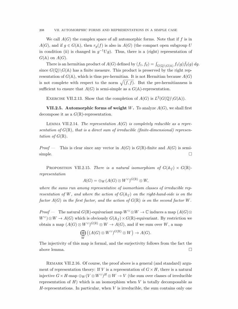
208 VII. AUTOMORPHIC FORMS AND REPRESENTATIONS IN A SIMPLE CASE
We call A(G) the complex space of all automorphic forms. Note that if f is in
A(G), and if g ∈ G(A), then rg(f) is also in A(G) (the compact open subgroup U
in condition (ii) is changed in g−1Ug). Thus, there is a (right) representation of
G(A) on A(G).
There is an hermitian product ofA(G) defined by (f1, f2) =∫G(Q)\G(A) f1(g)f2(g) dg.
since G(Q)\G(A) has a finite measure. This product is preserved by the right rep-
resentation of G(A), which is thus pre-hermitian. It is not Hermitian because A(G)
is not complete with respect to the norm»
(f, f). But the pre-hermitianness is
sufficient to ensure that A(G) is semi-simple as a G(A)-representation.
Exercise VII.2.13. Show that the completion of A(G) is L2(G(Q)\G(A)).
VII.2.5. Automorphic forms of weight W . To analyze A(G), we shall first
decompose it as a G(R)-representation.
Lemma VII.2.14. The representation A(G) is completely reducible as a repre-
sentation of G(R), that is a direct sum of irreducible (finite-dimensional) represen-
tation of G(R).
Proof — This is clear since any vector in A(G) is G(R)-finite and A(G) is semi-
simple.
Proposition VII.2.15. There is a natural isomorphism of G(Af ) × G(R)-
representation
A(G) = ⊕W (A(G)⊗W∨)G(R) ⊗W,
where the sums run among representative of isomorhism classes of irreducible rep-
resentation of W , and where the action of G(Af ) on the right-hand-side is on the
factor A(G) in the first factor, and the action of G(R) is on the second factor W .
Proof — The natural G(R)-equivariant map W∨⊗W → C induces a map (A(G)⊗W∨)⊗W → A(G) which is obviously G(Af )×G(R)-equivariant. By restriction we
obtain a map (A(G)⊗W∨)G(R) ⊗W → A(G), and if we sum over W , a map⊕W
Ä(A(G)⊗W∨)G(R) ⊗W
ä→ A(G).
The injectivity of this map is formal, and the surjectivity follows from the fact the
above lemma.
Remark VII.2.16. Of course, the proof above is a general (and standard) argu-
ment of representation theory: If V is a representation of G×H, there is a natural
injective G×H-map ⊕W (V ⊗W∨)H ⊗W → V (the sum over classes of irreducible
representation of H) which is an isomorphism when V is totally decomposable as
H-representations. In particular, when V is irreducible, the sum contains only one

VII.2. AUTOMORPHIC FORMS AND AUTOMORPHIC REPRESENTATIONS 209
non-zero term, and V = Z⊗W , where W is an irreducible representation of H and
Z = (V ⊗W∨)H is an irreducible representation of G.
We know analyze the G(Af )-representation (A(G)⊗W∨)G(R).
Definition VII.2.17. We denote A(G,W ) the space of functions f : G(Af )→W ∗ such that
(i) The function f satisfies, for all γ ∈ G(Q) and all g ∈ G(Af ), f(γg) =
f(g)|γ−1∞
, where γ∞, the canonical image of γ in G(R) acts on f(g) ∈ W∨
using the right representation of G(R) on W∨.
(ii) The function f is right-invariant by some open compact subgroup U of
G(Af ) (U depends on f).
Such functions are called automorphic forms of weight W .
Obviously A(G,W ) is a right smooth G(Af )-representation
Proposition VII.2.18. There is a natural isomorphism of G(Af )-representation
(induced by the restriction from G(A) to G(Af ))
(A(G)⊗W )G(R) = A(G,W )
Proof — First, (A(G)⊗W∨)G(R) is trivially identified with the space of functions
f : G(A)→W∨ satisfying:
(i) The function f is left-invariant under G(Q).
(ii) The function f is right-invariant by some open compact subgroup U of
G(Af ) (U depends on f).
(iii) The function f is G(R)-covariant on the right: that is, f(gh) = f(g)|h for
g ∈ G(A), h ∈ G(R).
Start with an f as above and define f ′ : G(Af )→ W ∗ by restriction. Then we
have for γ ∈ G(Q) and g ∈ G(Af ),
f ′(γg) = f((γg, 1∞)) (by definition of f ′)
= f(γ(g, 1)γ−1∞ )
= f((g, 1))|γ−1∞
using (i) and (iii)
= f ′(g)|γ−1∞
Hence f ′ ∈ A(G,W ). Conversely, given an f ′ ∈ A(G,W ), there is a unique way to
extend it to an map f : G(A) → W∨ satisfying (i), (ii) and (iii) above, namely by
setting f(g, g∞) = f ′(g)|g−1∞
. Checking that f actually is in (A(G)⊗W )G(R) is the
same computation as above.
Remark VII.2.19. The proof of this proposition is a very standard trick in the
theory of automorphic forms. It is important to understand it completely.

210 VII. AUTOMORPHIC FORMS AND REPRESENTATIONS IN A SIMPLE CASE
Proposition VII.2.20. For every compact open subgroup U ⊂ G(Af ), the space
A(G,W )U is finite dimensional. In other words, the representation A(G,W ) is
admissible.
Proof — A function f ∈ A(G,W )U is completely determined by its value in W ∗
on a set of representatives in G(Af ) of the quotient G(Q)\G(Af )/U . This set is
finite by Cor. ??. Since W is finite dimensional the result follows.
There is also a pre-hermitian product on A(G,W ). Choose ( , )W∨ a G(R)-
invariant hermitian product on W∨ (such an Hermitian product exists since G(R)
is compact, and is unique up to multiplication by a scalar since W ∗ is irreducible).
The we define, for f.f ′ ∈ A(G,W ):
(f, f ′) =
∫G(Q)\G(Af )
(f(g), f ′(g))W∨ dg
which makes sense since (f(γg), f ′(γg))W∨ = (f(g)|γ−1∞, f ′(g)|γ−1
∞)W∨ = (f(g), f ′(g))W ′
so the integrand is a function on G(Q)\G(Af ). Hence A(G,W ) is semi-simple as a
G(Af )-representation.
VII.2.6. Automorphic representations.
Theorem VII.2.21. The representation A(G,W ) is a direct sum of irreducible
representation of G(Af ) with finite multiplicity.
Proof — This follows from the semi-simplicty of A(G,W ) just seen and its ad-
missibility (Prop. VII.2.20) in view of Prop VII.1.13.
Corollary VII.2.22. There is a decomposition
A(G) = ⊕m(π)π
as G(A) = G(Af ) × G(R)-representations, where the π = πf ⊗ π∞ are irreducible
representations of G(A), with pif an irreducible admissible representation of G(Af )
and π∞ being a (finite-dimensional) irreducible representation of G(R). Moreover
the multipliicty m(π) are finite.
This follows from the Theorem and Prop. VII.2.15.
Definition VII.2.23. An irreducible representation π of G(A) that appears in
the decomposition of A(G) is said automorphic. The number m(π) is called its
(automorphic) multiplicity. The component πl of πf (for l a prime), and π∞ are
called the local component of π. The equivalence class of the component π∞ is also
called the weight of π.

VII.3. A FRAGMENT OF THE THEORY OF ADMISSIBLE REPRESENTATION OF GLn OF A LOCAL FIELD211
VII.2.7. The automorphic representations are algebraic. Let π be an
automorphic representation and set W = π∞ be its weight, a representation of
G(R). Let us recall an elementary lemma of representation theory:
Lemma VII.2.24. Assume G(R) is compact, and G is reductive.
(i) The restriction by the map G(R) → G(C) induces a bijection between
the equivalence classes of complex algebraic representations of G(C) and
complex irreducible continuous representations of G(R).
(ii) If W is any irreducible finite-dimensional representation of G(R), the re-
striction of G(R) to G(Q) has a model WQ over Q.
From this we deduce easily
Proposition VII.2.25. The admissible G(Af )-representation A(G,W ) is de-
fined over Q. So are the πf for π any automorphic representations.
Proof — Just define A(G,W )Q as the space of functions f : G(Af ) → W ∗Q such
that
(i) The function f satisfies, for all γ ∈ G(Q) and all g ∈ G(Af ), f(γg) =
f(g)|γ−1 .
(ii) The function f is right-invariant by some open compact subgroup U of
G(Af ) (U depends on f).
This is clearly an admissible representation over Q, and tensorizing it by C gives
back A(G,W ), which proves the first assertion. The second follows form the first
by Exercise VII.1.9
VII.2.8. Levels.
Definition VII.2.26. A level U is
VII.3. A fragment of the theory of admissible representation of GLn of
a local field
In this subsection, let F be an extension of Ql, and G = GLn(F ), which is a
lctd group.
VII.3.1. Some algebraic subgroups, and the Bruhat decomposition.
First do the following easy exercise in group theory:
Exercise VII.3.1. Let G be a group, and A and B be two subgroups (not
necessarily normal). Show that the following are equivalent:
(i) AB = G
(ii) BA = G
(iii) A′B′ = G where A′ (resp. B′) is a conjugate of A (resp. of B) in G.

212 VII. AUTOMORPHIC FORMS AND REPRESENTATIONS IN A SIMPLE CASE
We let B the subgroup of upper triangular matrices in G (a Borel), N the sub-
group of upper triangular matriceswhose diagonal coefficients are 1 (the unipotent
radical of B) and T the subgroup of diagonal matrices (a maximal split torus)
Exercise VII.3.2. (easy) Show that N = [B,B]; in particular N is normal in
B. Show that B = NT , and N ∩ T = 1. In particular, there is a natural split
exacts equence 1→ N → B → T → 1 and T is abelianization of B.
Let W be the group of matrices whose coefficients are only 1 or 0, and with
exactly one 1 on each row and each column. Obviously W acts by permutation on
the standard basis of Fn and is thus naturally isomorphic to Sn. Also W acts by
conjugation on T .
Proposition VII.3.3 (Bruhat’s decomposition). One has
G =∐w∈W
BwB.
In other words, W is a set of representatives of B\G/B.
Proof — To give a conceptual proof, let’s introduce some terminology:
Let V = Fn. A flag in Fn is a family 0 = V0 ⊂ V1 ⊂ · · · ⊂ Vn−1 · · · ⊂ Vn = n
where each Vi is a subspace of V of dimension i. For example, taking Vi the space
generated by the i first elements of the canonical basis of Fn defines a flag F0.
The group G has a left t action on the sets of flags, defined by g(V0, V1, . . . , Vn) =
(gV0, gV1, . . . , gVm) and B is just the stabilizer of F0 for that action action. More-
over it is easy to see that G acts transitively on the set of flags so the map g 7→ gF0
is easily seen to be an isomorphism of G-sets from G/B onto the set of flags.
A lines decomposition is a set of n lines in V whose sum is V . For example, the
set of lines generated by a vector of the canonical basis is a lines decomposition L0.
We say that a lines decomposition belongs to a flag (V0, V1, . . . , Vn) if every of
the Vi is a sum of (necessarily i) lines of the line decomposition. For example L0
belongs to F0, and more generally, the lines decomposition that belongs to L0 are
the lines decomposition bL0 for b ∈ B.
The flags in which a line decomposition belong are clearly in bijection with the
ordering of the n lines of the line decomposition (the flag attached to an ordering
L1, . . . , Ln of lines is 0 ⊂ L1 ⊂ L1 ⊕ L2 ⊂ . . . ). In particular there are n! of them.
Now the key and easy fact is that for any two flags F and F ′ there exists a line
decomposition that belongs to both of them. This is left as an exercise.
In particular, if g ∈ G, then there is a line decomposition L belongings to both
F0 and gF0. Since L belongs to F0, it is of the form bL0ome b ∈ B. The flags F0
and F defines two ordering of the lines of L, hence of L0, and there is a permutation
matrix w ∈ W that transform the first ordering into the second : it follows that
bwF0 = gF0 and bwb′ = g for some b′ ∈ B. Thus G = ∪w∈WBwB. That the union
is disjoint is easy.
VII.4. AUTOMORPHIC REPRESENTATIONS FOR A FORM OF GLn THAT IS COMPACT AT INFINITY213
VII.3.2. Normalized induction.
VII.3.3. The Jacquet functor and decomposition of principal series.
VII.3.4. Maximal compact subgroups, Iwahoris, and the Iwasawa’s
decomposition.
VII.3.5. The spherical Hecke algebras, the Iwahori-Hecke algebra,
and the Atkin-Lehner algebra.
VII.3.6. Unramified representation.
VII.3.7. Refinements of unramifed representations.
VII.4. Automorphic representations for a form of GLn that is compact
at infinity
In this subsection, we assume that G is an algebraic group over Q such that
(a) G(R) is compact.
(b) GC ' GLn.
Hypothesis (b) implies that G is reducible and connected, hence the results of the
above subsection still apply here. There is a classification of the group satisfying
(b) (cf [?] or [?]).
VII.4.1. Classification of weights. As we have seen

CHAPTER VIII
Chenevier’s eigenvarieties
215


CHAPTER IX
A p-adic L-function on unitary eigenvariety and its zerolocus
217


CHAPTER X
Solution to exercises
Solution to Exercise I.1.1 See [E, Proposition 2.10].
Solution to Exercise I.1.2 See the solution to Exercise I.4.2.
Hint to Exercise I.1.3 By construction of the characteristic polynomial, this
question reduces to the case where M is free, in which case it is trivial.
Solution to Exercise I.3.3 The surjective tautological mapH⊗R→ TA factors
through T since any element h ∈ H⊗R such that ψ(h) = 0 obviously acts by 0 on
A. Hence we have a natural surjective map T → TA. Its kernel is by construction
the ideal generated by the elements ψ(h) of EndRM than vanish on A. If M/A is
torsion, such an endomorphism ψ(h) is torsion in EndR(M), hence is 0 if R is a
domain because in this case EndR(M) is torsion free. This proves 1.
For 2. and an example of non-injectivity, takes A = B = 0. For an example
of non-surjectivity, take A = B = R and M = A ⊕ B with H generated by one
element T which acts as the identity on M . Then the map T → TA × TB is the
diagonal embedding R→ R2 which is not surjective.
3. is proved exactly as the second part of 1.
For 4. let e = (T − a)/(b − a) in T , so e acts by 0 on A and 1 and B, that is
the image of e ∈ T is 0 in TA and 1 in TB. If tA ∈ TA and tB ∈ TB, there exists
uA ∈ T that maps on tA in TA (since the map T → TA is surjective by 1.) and
uB ∈ T that maps on tB in TB (same reason). Then t := (1− e)tA + etB ∈ T maps
to (tA, tB) in TA × TB.
Hint to Exercise I.3.4 For 1. consider the map T → T ∨ that sends an endo-
morphism of M to its transpose.
2. is just a reformulation of the classical result that over any field a square
matrix is conjugate to its transpose.
For 3. and R not a field, check that one just need to find a matrix in Mn(R)
which is not conjugate (in GLn(R)) to its transpose. Then check that for R = Z,
the matrix T =
Ç1 −53 −1
åis not similar to its transpose over Z.
219
220 X. SOLUTION TO EXERCISES
For 3. and R = C, take M = C3 and H generated by two elements X and Y
acting on M by the matrices X =
Ñ0 0 01 0 00 0 0
éand Y =
Ñ0 0 00 0 01 0 0
é.
Solution to Exercise I.3.4 1. and 2. should be clear after the hint.
For 3. and the case of a ring, checking that the matrix T =
Ç1 −53 −1
å∈ M2(Z)
is not conjugate to its transpose is a straightforward but tedious computation. For
a conceptual proof, and an explanation of how this example was found and how to
find many other ones, see [ConK], especially Example 15.
For 3. and the case of a field, considering the example given in the hint we
observe that ImY ⊕ ImX has dimension 2 while Im tY ⊕ Im tX has dimension
1. There can therefore be no matrices P ∈ GL3(C) such that PXP−1 = tX and
PY P−1 = tY , which shows that as an H-module, M is not isomorphic to M∨.
Solution to Exercise I.3 For 1. let M = R2, and ψ : a + bε 7→Ça b0 a
åfor
a ∈ R, b ∈ I. For 2. take R = C[X,Y ]. Since R is regular of dimension 2, any
finite torsion-free R-algebra is an eigenalgebra, and there are plenty of them that
are non-flat.
Solution to Exercise I.4.2 The eigenalgebra T is the quotient of Zp[T ] by the
ideal of operators that act trivially on M . Let P (X) ∈ Zp[X]. If P (T ) = 0 as an
operator on M , then P is divisible by the minimal polynomial (X − 1)2 of T in
Qp[X], so is divisible by (X−1)2 in Zp[X] (since the algorithm of euclidean division
by a monic polynomial like (X − 1)2 is identical in Zp[X] and Qp[X]). It follows
that T ' Zp[X]/(X − 1)2 with the isomorphism sending T on X.
The eigenalgebra T ′ is simply Fp since T acts as the identity on M ⊗ Fp = F2p.
The map T ⊗Zp Fp = Fp[X]/(X − 1)2 → T ′ = Fp is the map that sends X on 1. Of
course this map is not an isomorphism.
Solution to Exercise I.5.4 This is standard: by induction on the number
of generators of ψ(H), one reduces to the case of one generator T of ψ(H). In
this case let P (X) be the characteristic (or minimal) polynomial of T and write
P (X) = (X−a1)n1 . . . (X−ar)nr where the ai are distinct. Let Pi(X) be the same
polynomial with the factor (X − ai)ni removed. Then the Pi’s are relatively prime,
and a Bezout relation between them shows that M =∑i ker(T−ai)ni , a sum which
is obviously direct.
Solution to Exercise I.5.5 We obviously have M [χ] ⊗ k′ ⊂ M ′[χ′] in M ′ and
the equality follows from the equality of dimensions, since the rank of a system of
linear equations over k does not change when we extend the scalar to k′. Same
argument for M(χ).
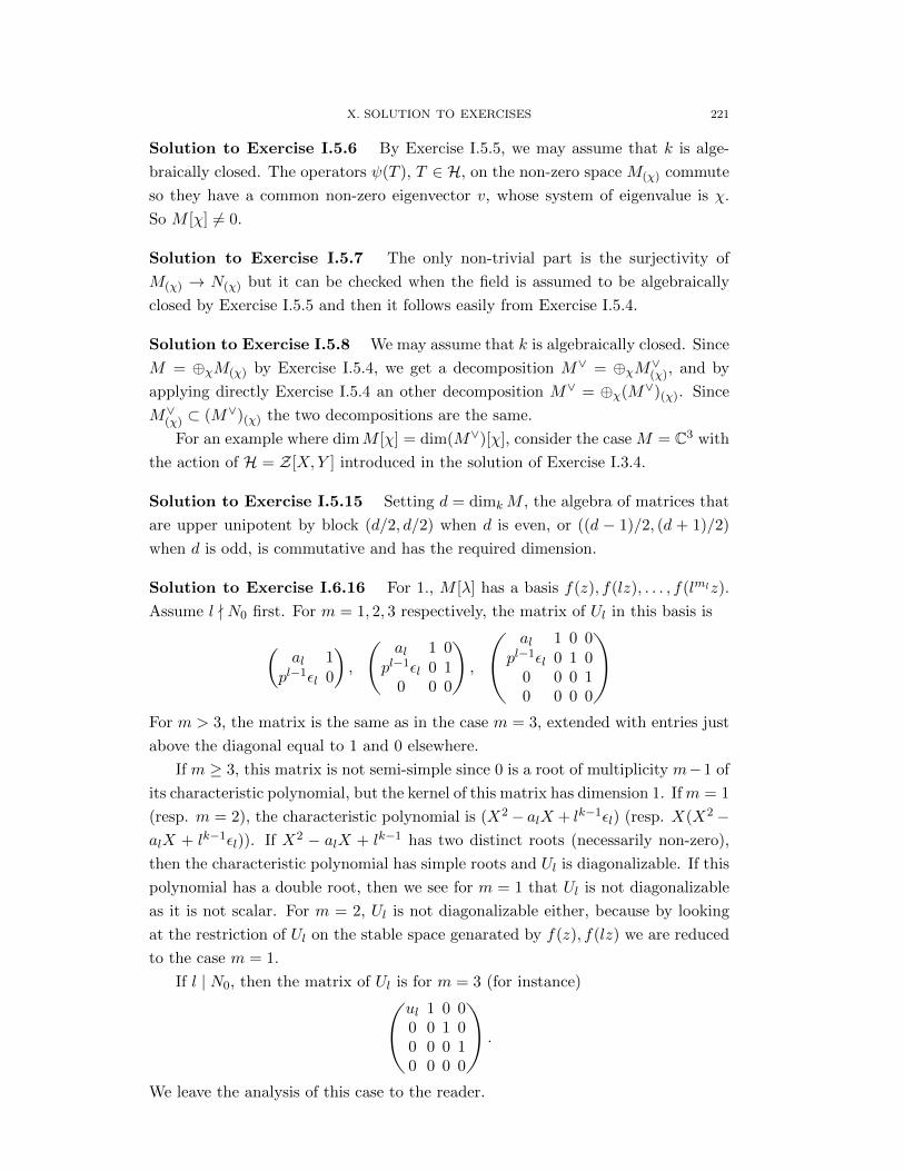
X. SOLUTION TO EXERCISES 221
Solution to Exercise I.5.6 By Exercise I.5.5, we may assume that k is alge-
braically closed. The operators ψ(T ), T ∈ H, on the non-zero space M(χ) commute
so they have a common non-zero eigenvector v, whose system of eigenvalue is χ.
So M [χ] 6= 0.
Solution to Exercise I.5.7 The only non-trivial part is the surjectivity of
M(χ) → N(χ) but it can be checked when the field is assumed to be algebraically
closed by Exercise I.5.5 and then it follows easily from Exercise I.5.4.
Solution to Exercise I.5.8 We may assume that k is algebraically closed. Since
M = ⊕χM(χ) by Exercise I.5.4, we get a decomposition M∨ = ⊕χM∨(χ), and by
applying directly Exercise I.5.4 an other decomposition M∨ = ⊕χ(M∨)(χ). Since
M∨(χ) ⊂ (M∨)(χ) the two decompositions are the same.
For an example where dimM [χ] = dim(M∨)[χ], consider the case M = C3 with
the action of H = Z[X,Y ] introduced in the solution of Exercise I.3.4.
Solution to Exercise I.5.15 Setting d = dimkM , the algebra of matrices that
are upper unipotent by block (d/2, d/2) when d is even, or ((d − 1)/2, (d + 1)/2)
when d is odd, is commutative and has the required dimension.
Solution to Exercise I.6.16 For 1., M [λ] has a basis f(z), f(lz), . . . , f(lmlz).
Assume l - N0 first. For m = 1, 2, 3 respectively, the matrix of Ul in this basis isÇal 1
pl−1εl 0
å,
Ñal 1 0
pl−1εl 0 10 0 0
é,
Üal 1 0 0
pl−1εl 0 1 00 0 0 10 0 0 0
êFor m > 3, the matrix is the same as in the case m = 3, extended with entries just
above the diagonal equal to 1 and 0 elsewhere.
If m ≥ 3, this matrix is not semi-simple since 0 is a root of multiplicity m−1 of
its characteristic polynomial, but the kernel of this matrix has dimension 1. Ifm = 1
(resp. m = 2), the characteristic polynomial is (X2− alX + lk−1εl) (resp. X(X2−alX + lk−1εl)). If X2 − alX + lk−1 has two distinct roots (necessarily non-zero),
then the characteristic polynomial has simple roots and Ul is diagonalizable. If this
polynomial has a double root, then we see for m = 1 that Ul is not diagonalizable
as it is not scalar. For m = 2, Ul is not diagonalizable either, because by looking
at the restriction of Ul on the stable space genarated by f(z), f(lz) we are reduced
to the case m = 1.
If l | N0, then the matrix of Ul is for m = 3 (for instance)Üul 1 0 00 0 1 00 0 0 10 0 0 0
ê.
We leave the analysis of this case to the reader.
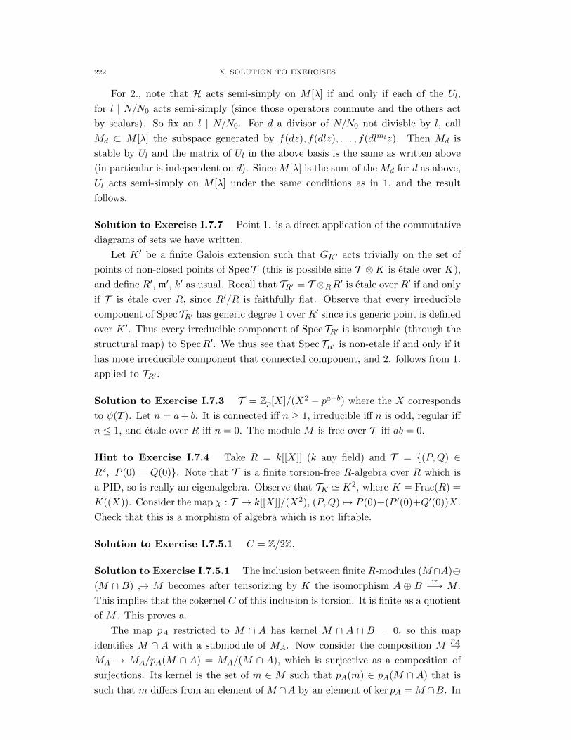
222 X. SOLUTION TO EXERCISES
For 2., note that H acts semi-simply on M [λ] if and only if each of the Ul,
for l | N/N0 acts semi-simply (since those operators commute and the others act
by scalars). So fix an l | N/N0. For d a divisor of N/N0 not divisble by l, call
Md ⊂ M [λ] the subspace generated by f(dz), f(dlz), . . . , f(dlmlz). Then Md is
stable by Ul and the matrix of Ul in the above basis is the same as written above
(in particular is independent on d). Since M [λ] is the sum of the Md for d as above,
Ul acts semi-simply on M [λ] under the same conditions as in 1, and the result
follows.
Solution to Exercise I.7.7 Point 1. is a direct application of the commutative
diagrams of sets we have written.
Let K ′ be a finite Galois extension such that GK′ acts trivially on the set of
points of non-closed points of Spec T (this is possible sine T ⊗K is etale over K),
and define R′, m′, k′ as usual. Recall that TR′ = T ⊗RR′ is etale over R′ if and only
if T is etale over R, since R′/R is faithfully flat. Observe that every irreducible
component of Spec TR′ has generic degree 1 over R′ since its generic point is defined
over K ′. Thus every irreducible component of Spec TR′ is isomorphic (through the
structural map) to SpecR′. We thus see that Spec TR′ is non-etale if and only if it
has more irreducible component that connected component, and 2. follows from 1.
applied to TR′ .
Solution to Exercise I.7.3 T = Zp[X]/(X2 − pa+b) where the X corresponds
to ψ(T ). Let n = a+ b. It is connected iff n ≥ 1, irreducible iff n is odd, regular iff
n ≤ 1, and etale over R iff n = 0. The module M is free over T iff ab = 0.
Hint to Exercise I.7.4 Take R = k[[X]] (k any field) and T = (P,Q) ∈R2, P (0) = Q(0). Note that T is a finite torsion-free R-algebra over R which is
a PID, so is really an eigenalgebra. Observe that TK ' K2, where K = Frac(R) =
K((X)). Consider the map χ : T 7→ k[[X]]/(X2), (P,Q) 7→ P (0)+(P ′(0)+Q′(0))X.
Check that this is a morphism of algebra which is not liftable.
Solution to Exercise I.7.5.1 C = Z/2Z.
Solution to Exercise I.7.5.1 The inclusion between finite R-modules (M∩A)⊕(M ∩ B) → M becomes after tensorizing by K the isomorphism A ⊕ B '−→ M .
This implies that the cokernel C of this inclusion is torsion. It is finite as a quotient
of M . This proves a.
The map pA restricted to M ∩ A has kernel M ∩ A ∩ B = 0, so this map
identifies M ∩ A with a submodule of MA. Now consider the composition MpA→
MA → MA/pA(M ∩ A) = MA/(M ∩ A), which is surjective as a composition of
surjections. Its kernel is the set of m ∈ M such that pA(m) ∈ pA(M ∩ A) that is
such that m differs from an element of M ∩A by an element of ker pA = M ∩B. In
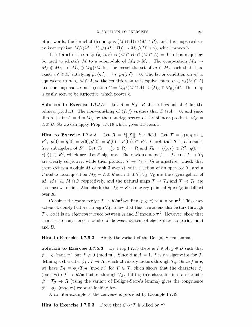
X. SOLUTION TO EXERCISES 223
other words, the kernel of this map is (M ∩ A)⊕ (M ∩ B), and this maps realizes
an isomorphism M/((M ∩A)⊕ (M ∩B))→MA/(M ∩A), which proves b.
The kernel of the map (pA, pB) is (M ∩ B) ∩ (M ∩ A) = 0 so this map may
be used to identify M to a submodule of MA ⊕ MB. The composition MA →MA ⊕MB → (MA ⊕MB)/M has for kernel the set of m ∈ MA such that there
exists m′ ∈ M satisfying pA(m′) = m, pB(m′) = 0. The latter condition on m′ is
equivalent to m′ ∈ M ∩ A, so the condition on m is equivalent to m ∈ pA(M ∩ A)
and our map realizes an injection C = MA/(M ∩A)→ (MA ⊕MB)/M . This map
is easily seen to be surjective, which proves c.
Solution to Exercise I.7.5.2 Let A = Kf , B the orthogonal of A for the
bilinear product. The non-vanishing of 〈f, f〉 ensures that B ∩ A = 0, and since
dimB + dimA = dimMK by the non-degeneracy of the bilinear product, MK =
A⊕B. So we can apply Prop. I.7.16 which gives the result.
Hint to Exercise I.7.5.3 Let R = k[[X]], k a field. Let T = (p, q, r) ∈R3, p(0) = q(0) = r(0), p′(0) = q′(0) + r′(0) ⊂ R3. Check that T is a torsion-
free subalgebra of R3. Let TA = p ∈ R = R and TB = (q, r) ∈ R2, q(0) =
r(0) ⊂ R2, which are also R-algebras. The obvious maps T → TA and T → TBare clearly surjective, while their product T → TA × TB is injective. Check that
there exists a module M of rank 3 over R, with a action of an operator T , and a
T -stable decomposition MK = A⊕B such that T , TA, TB are the eigenalgebras of
M , M ∩ A, M ∩ B respectively, and the natural maps T → TA and T → TB are
the ones we define. Also check that TK = K3, so every point of Spec TK is defined
over K.
Consider the character χ : T → R/m2 sending (p, q, r) to p mod m2. This char-
acters obviously factors through TA. Show that this characters also factors through
TB. So it is an eigencongruence between A and B modulo m2. However, show that
there is no congruence modulo m2 between system of eigenvalues appearing in A
and B.
Hint to Exercise I.7.5.3 Apply the variant of the Deligne-Serre lemma.
Solution to Exercise I.7.5.3 By Prop I.7.15 there is f ∈ A, g ∈ B such that
f ≡ g (mod m) but f 6≡ 0 (mod m). Since dimA = 1, f is an eigenvetor for T ,
defining a character φf : T → R, which obviously factors through TA. Since f ≡ g,
we have Tg ≡ φf (T )g (mod m) for T ∈ T , shich shows that the character φf
(mod m) : T → R/m factors through TB. Lifting this character into a character
φ′ : TB → R (using the variant of Deligne-Serre’s lemma) gives the congruence
φ′ ≡ φf (mod m) we were looking for.
A counter-example to the converse is provided by Example I.7.19
Hint to Exercise I.7.5.3 Prove that OM/T is killed by πv.
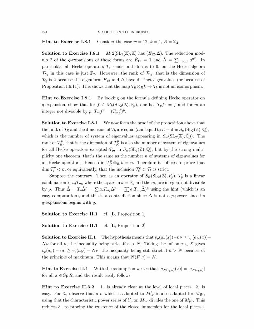
224 X. SOLUTION TO EXERCISES
Hint to Exercise I.8.1 Consider the case w = 12, k = 1, R = Z2.
Solution to Exercise I.8.1 M12(SL2(Z),Z) has (E12,∆). The reduction mod-
ulo 2 of the q-expansions of those forms are E12 = 1 and ∆ =∑n odd qn
2. In
particular, all Hecke operators Tp sends both forms to 0, on the Hecke algebra
TF2 in this case is just F2. Howewer, the rank of TZ2 , that is the dimension of
TQ is 2 because the eigenform E12 and ∆ have distinct eigenvalues (or because of
Proposition I.6.11). This shows that the map TR⊗Rk → Tk is not an isomorphism.
Hint to Exercise I.8.1 By looking on the formula defining Hecke operator on
q-expansion, show that for f ∈ Mk(SL2(Z),Fp), one has Tpfp = f and for m an
integer not divisible by p, Tmfp = (Tmf)p.
Solution to Exercise I.8.1 We now form the proof of the proposition above that
the rank of TR and the dimension of Tk are equal (and equal to n = dimSw(SL2(Z),Q),
which is the number of system of eigenvalues appearing in Sw(SL2(Z), Q)). The
rank of T pR , that is the dimension of T pK is also the number of system of eigenvalues
for all Hecke operators excepted Tp, in Sw(SL2(Z), Q), but by the strong multi-
plicity one theorem, that’s the same as the number n of systems of eigenvalues for
all Hecke operators. Hence dim T pR ⊗R k = n. Therefore it suffices to prove that
dim T pk < n, or equivalently, that the inclusion T pk ⊂ Tk is strict.
Suppose the contrary. Then as an operator of Sw(SL2(Z), Fp), Tp is a linear
combination∑aiTmi where the ai are in k = Fp,and themi are integers not divisible
by p. Thus ∆ = Tp∆p =
∑aiTmi∆
p = (∑aiTmi∆)p using the hint (which is an
easy computation), and this is a contradiction since ∆ is not a p-power since its
q-expansions begins with q.
Solution to Exercise II.1 cf. [L, Proposition 1]
Solution to Exercise II.1 cf. [L, Proposition 2]
Solution to Exercise II.1 The hypothesis means that vp(an(x))−nν ≥ vp(aN (x))−Nν for all n, the inequality being strict if n > N . Taking the inf on x ∈ X gives
vp(an) − nν ≥ vp(aN ) − Nν, the inequality being still strict if n > N because of
the principle of maximum. This means that N(F, ν) = N .
Hint to Exercise II.1 With the assumption we see that |aN(Q,ν)(x)| = |aN(Q,ν)|for all x ∈ SpR, and the result easily follows.
Hint to Exercise II.3.2 1. is already clear at the level of local pieces. 2. is
easy. For 3., observe that a ν which is adapted to M ′W is also adapted for MW ,
using that the characteristic power series of Up on MW divides the one of M ′W . This
reduces 3. to proving the existence of the closed immersion for the local pieces (

X. SOLUTION TO EXERCISES 225
EW,ν → E ′W,ν , which is easy. For 4., apply 3. twice and observe that the eigenvariety
for M2W is the same as for MW .
Solution to Exercise II.4 A system of eigenvalues appearing in M ′′W apears
either in MW or in M ′W . Hence the exercise follows from the above theorem.
Solution to Exercise II.5.1 In an irreducible one-dimensional rigid analytic
subspace, any set with an accumulation point is Zariski-dense. In particular a+ bNis Zariski dense. If x ∈ a+bN, and V is an affinoid closed ball of radius r > 0 around
a, then for n big enough x + pnbN ∈ V ∩ X and those set has x as accumulation
point.
Solution to Exercise III.1.1 1.a. Let A,B,C be such a triangle. Let D be the
point such that (ABDC) is a parallelogram. Then there is no points of Z2 in that
paralellogram, except A,B,C and D since any point in (ABDC) either lies on the
triangle (ABC) or on the triangle (BCD) in which case the symmetric of P with
respect to the middle of (BC) would be an integral point in (ABC).
We can assume that that A is the origin (0, 0) by translation. Let Λ be the
lattice in R2 generated by the vectors ~AB, ~AC. Clearly Λ ⊂ Z2. We claim that
this inclusion is an equality. Indeed, if P ∈ Z2, there is v ∈ Λ such that p − v lies
in the parallelogram (ABCD). Since p− v is in Z2, it is by the above either A, B,
C or D. In any case p− v ∈ Λ so p ∈ Λ.
It follows that the vectors ~AB, ~AC generates Z2. Hence their determinant is
±1, and the area of the triangle (ABC) is 1/2,
1.b. Let A = (0, 0), B = (a, c), C = (b, d). Assume that the angle ~AB, ~AC is
less than 180 degrees by exchanging B and C if necessary. If the triangle (A,B,C)
has area 1/2, the matrix γ
Ça bc d
åhas determinant ±1, and actually 1 by our angle
hypothesis. Thus γ ∈ SL2(Z) sends ∞ − 0 to a/c − b/d1.c. Let A = (0, 0), B = (a, c), C = (b, d). Assume that the angle ~AB, ~AC is
less than 180 degrees by exchanging B and C if necessary. We prove by induction
on the number of points of Z2 in the triangle (ABC) that a/c− b/d lies in the
Z[SL2(Z)]-module generated by ∞ − 0. Since those divisors clearly generate
∆0 as Z-module, this would be sufficient to prove Manin’s lemma.
To start the induction, note that when (ABC) has only three points in Z2, we
know that it has area 1/2 by 1.a. So by 1.b. we are done.
In general, if (ABC) has more than three points in Z2, let D = (e, f) be a
fourth point. By replacing D by an other point of Z2 in the segment [AD] (which
lies inside the triangle (ABC)), we can assume that e and f are relatively prime
integers. Note that D is not on [AB] (resp. nor on [AC]) since we have assumed
that a and c (resp. b and d) are relatively prime. Therefore the triangles (ABD)
and (ADC) are non-flat, and have strictly less integral points that (ABC). By

226 X. SOLUTION TO EXERCISES
induction hypothesis, we know that a/c − e/f and e/f − b/d both belong
to the Z[SL2(Z)]-module generated by ∞ − 0). So their sum also does, which
proves the induction step.
2. follows from easily from 1. using that SL2(Z)/Γ is finite.
3. By induction on the number of integral points in a polygon, any (reasonable)
polygon can be covered by triangles whose vertices are in Z2 and that contain no
other point of Z2. Since we know by a. that Pick’s theorem is true for any of
those triangles, it is sufficient to check that Pick’s theorem is additive, that is holds
for any polygon with vertices in Z2 that is the union of two smaller polygon with
vertices in Z2, disjoint interior, and an edge in common, provided Pick’s theorem
is true for those two smaller polygons. This is an easy computation. We leave the
details to the reader.
Hint to Exercise III.1.2 If this is difficult, read or re-read the chapter on Hecke
operators in [Shi]
Solution to Exercise III.1.2 We have
Γ
Ç1 00 l
åΓ =
l−1∐a=0
Ç1 a0 l
å∐Çl 00 1
åfor l - N and the same without the last matrix if l | N . Since all those matrices
have determinant l, the result follows from the definition of the Hecke operators.
Hint to Exercise III.1.3 Look up a good reference in algebraic topology.
Solution to Exercise III.1.4 The image of (x0, y0) by (22) only depends on
x = β(x0) by the commutativity of (23). To see it only depends on y = β(y0),
exchange G with G∨ and i with n− i.
Solution to Exercise III.1.4 By exhanging G with G∨, we only need to show
that for x ∈ H i! (X,G
∨), there is a y ∈ Hn−i! (X,G) such that (x, y) 6= 0. Seeing x as
an element of H i(X,G∨), there is by the non-degeneracy of (21) a y0 ∈ H1c (X,G∨)
such that (x, y0) 6= 0. Setting y = β(y0), we have (x, y) 6= 0.
Solution to Exercise III.2.5 No, we have dimCW [χ] = dimC W [χ].
Solution to Exercise III.2.5 The map c is clearly R-linear, so we only need to
check that c(iw) = ic(w). If w = w1 + iw2 with w1, w2 ∈WR, then iw = −w2 + iw1,
so c(iw) = −w2 + iw1 = i(w1 + iw2) = ic(w).
Hint to Exercise III.2.8 Γ0(N) has 2r cusps, which are parametrized by the
application from a : l1, . . . , lr → 0, 1; if c is such an application, the set ca
of rational numbers which are l-integral (resp. not l-integral) if a(l) = 1 (resp.
a(l) = 0) is a Γ0(N)-class in P1(Q).)
X. SOLUTION TO EXERCISES 227
Solution to Exercise III.3.1 In the definition of fχ(z), introducing the easy
equality χ(n) =
∑a(mod m)
χ(a)e2iπna/m
τ(χ) gives the formula for fχ(z). For the fact that
fχ(z) is a modular form, see [Shi, Prop. 3.64]
Solution to Exercise III.3.1 if ψ is any continuous character A∗Q/Q∗ → C∗,then ψ|R∗+ as the form x 7→ xs for some (unique) s ∈ C. Then ψ| |−s is a continuous
character on A∗Q/Q∗R+∗ and we conclude by Class Field Theory.
Solution to Exercise III.3.2 When m is prime to p, the polynomials (z −a/m)j are p-integral, so the right hand side of (??) is clearly p-integral. Let
us assume that k = 0. Then since φ±f are p-normalized, there is an irreducible
fraction a/m such that φf (∞ − a/m)/Ω±f has p-valuation 0. Thus by lin-
ear independence of characters, there is a character χ of conductor m such that∑a(mod m) χ(a)
φ±f
(∞−a/m)Ω±f
also has p-valuation zero.
Hint to Exercise III.4.2 Consult [BGR]
Solution to Exercise III.4.2 Choose a set E that satisfies the condition of
Prop. III.4.12 for both r1 and r2. Through the identifications A[r1](L) = cr1(L)E 'c(L)E and A[r2](L) = cr2(L)E ' c(L)E given by Corollary and ..., the restriction
map becomes the diagonal map c(L)E → c(L)E that on each component is the map
c(L)→ c(L), (an) 7→ ((r2/r1)nan). SInce (r2/r1)n goes to 0 when n goes to∞, this
map is compact by [Bu, Prop. 2.4].
Solution to Exercise III.5.1
Hint to Exercise III.5.3 See [CO2]
Hint to Exercise III.5.3 See [CO1]
Hint to Exercise III.5.3 This follows from the main results of [L, §3].
Hint to Exercise III.5.3 See [?]
Hint to Exercise III.5.3 The functions log+p (1 + x) and log−p (1 + x) defined in
[?] are good examples.
Solution to Exercise III.6.2 This is trivial.
Solution to Exercise III.6.3 Let an = pm = n+ 1 if n = pm− 1 for an integer
m, an = 0 otherwise. Then lim an = 0 so f(z) =∑anz
n ∈ A[1]. However, the
antiderivative g(z) =∑bnz
n of f has bpm = 1 for all m so g 6∈ A[1].
Solution to Exercise III.6.3 Why should it?
228 X. SOLUTION TO EXERCISES
Solution to Exercise III.6.3 For a., if d is an ultramteric distance that is
invariant by translation, then |x| := d(x, 0) is a norm: the first property is obvious,
and we have |x − y| = d(x − y, 0) = d(x, y) ≤ max(d(x, 0), d(0, y)) = max(|x|, |y|).Conversely, if | | is a norm, then | − x| = |0− x| ≤ |x| and by symmetry |x| = | − x|for all x. If then we set d(x, y) := |x−y|, then clearly one has d(x, y) = 0 if and only
if x = y; d(x, y) = d(y, x); d(x+ z, y + z) = d(x, y); and d(x, z) = |x− z| = |((x−y)− (z − y)| ≤ max(|x− y|, |z − y|) = max(d(x, y), d(z, y)) = max(d(x, y), d(y, z)).
For b., see [Sch, Prop. 8.1]
Solution to Exercise III.6.3 Points a. and c. are clear from the definition.
For point b., the canononical surjection π : X → X/ ker f is open: if U is open,
we need to show that π(U) is open which means that π−1(π(U)) = U + Kerf is
open, which is clear. Hence f = f π is open if and only if f is open. Since f is a
continuous isomorphism, it is open if and only if it is an homeomorphism. (After
[BGR, §1.1.9].)
For d., cf [BGR, §1.1.9]
For e., note that both X and Y are normable group by the above exercise. If f
is strict, f(X) ' X/ ker f is complete, hence closed in X. Connversely, if f(X) is
closed, it inherits a structure of Frechet, and the isomorphism f : X/ ker f → f(X)
is thus an homeomorphism by the open mapping theorem ([?, Prop. 8.6]).
For f., recall that f strict means that the continuous isomorphism f : X/ ker f →f(X) is an homeomorphism. The map f ′ : X ′/ ker f ′ → f ′(X ′) is just (f) ⊗ 1 by
flatness of R′ over R. Hence we are reduced to the case where f is an isomorphism.
In this case, that f is an homeomorphism means that for every semi-norm q in our
familiy of semi-norms on Y , one has two semi-norms p1 and p2 in our family on
X and two positive constant C1 and C2 such that C1p1 ≤ f∗q ≤ C2p2. But then
clearly C1p′1 ≤ f ′∗q′ ≤ C2p
′2 and it follows that f ′ is an homeomorphism.
Solution to Exercise III.6.3 This map is a morphism of Frechet space and
has a closed image by Theorem III.6.13. Therefore it is strict by point e. of
Exercise III.6.16.
Solution to Exercise III.6.5 Consider the following example: V = Q(N)p and Up
is the operator sending (u0, u1, u2, u3, u4, . . . ) to (u0, u0, u1, u2, u3, . . . ). Let W =
Qp with Up acting on it as the identity. Then the map V →W , (u0, u1, u2, . . . ) 7→ u0
is Up-equivariant and surjective, but V ≤0 →W≤0 is not surjective.
Solution to Exercise III.6.6 Similar to Exercise III.6.17.
Solution to Exercise III.7.1 One has f(pz) = p−1−kf|
Çp 00 1
å(z), and the
results follows from the fact that
Çp 00 1
åΓ
Çp 00 1
å−1
⊂ Γ1(N).
X. SOLUTION TO EXERCISES 229
Solution to Exercise III.7.3 To get from the first to the second line: we need
zj ∈ Pk.
Solution to Exercise IV.1.1 There is no solution: I don’t know the answer.
Solution to Exercise IV.1.2 After all, look in [BGR].
Hint to Exercise IV.4 Look up the appendix of [?].
Solution to Exercise IV.4 We have ρx = 1 ⊕ ωp. Since Up(x) = p, in a
neighborhood of x all classical point y are such that ρy is irreducible (cf. the
appendix of [?].) Hence by Ribet’s lemma ([?]) we can construct a non trivial
extension, in the category of GQ,lp-representations, of 1 by ωp, which is crystalline
at p by (iii) of Prop. IV.4.4. If there was infinitely many classical points y in the
given neighborhood of minimal tame level 1 (instead of l), then that extension
would also be unramified at l: but there is non-trivial extension of 1 by ωp in the
categroy of GQ-representations that is unramfied everywhere and crystalline at p,
because Q has only finitely many units (cf. the appendix of [?]).
Solution to Exercise VI.2.2 One has | logp κ(γ)| < 1 and | logp(γ)| = 1/p, so
| logp κ(γ)/ logp(γ)| < p. Hence∣∣∣(κi)∣∣∣ < pi|i!|−1. Since vp(i!) < i/(p − 1), |i!|−1 <
pi/(p−1) and the result follows.

Bibliography
[AB] M. Auslander & D.A. Buchsbaum, On ramification theory in noetherian rings, Amer. J.Math. 81 1959 749–765.
[AS] A. Ash & G. Stevens: Modular forms in characteristic l and special values of their L-functions, Duke Math, J 53(3), 849–868 (1986).
[AV] Y. Amice & J. Velu, Distributions p-adiques associees aux series de Hecke, JourneesArithmetiques de Bordeaux (Conf., Univ. Bordeaux, Bordeaux, 1974), pp. 119–131. As-terisque, Nos. 24-25, Soc. Math. France, Paris, 1975.
[B] J. Bellaıche, Critical p-adic L-function, to appear in inventiones mathematicae, 2012[B2] J. Bellaıche, Ribet’s lemma, generalizations, and pseudo-characters, notes from Hawaii CMI
summer school, available at the author’s webpage[BC] J. Bellaıche & G. Chenevier, Families of Galois representations and Selmer groups, Soc.
Math. France, Asterisque 324 (2009).[BD] J. Bellaıche & S. Dasgupta, the p-adic L-functions of evil Eisenstein series, preprint, sub-
mitted[1] BE C. Breuil & M. Emerton, Representations p-adiques ordinaires de GL2(Qp) et compat-
ibilite local-global, Asterisque No. 331 (2010), 255?315.[Bo] A. Borel, Some finiteness properties of adele groups over number fields, IHES Publ. math.
16 (1963), 5–30.[Bu] K. Buzzard, Eigenvarieties, Proc. of the LMS Durham Conference on L-functions and
arithmetic (2007).[BGR] S. Bosch, U. Guntzer & R. Remmert, Non-archimedian analysis, Springer Verlag,
Grundlehren der math. Wiss. 261 (1984).[Cara] H. Carayol, Sur les representations galoisiennes modulo l attachees aux formes modulaires.,
Duke Math. J. 59 (1989), no. 3, 785?801[Ca] P. Cartier, Representations of p-adic groups: a survey. Automorphic forms, representations
and L-functions (Proc. Sympos. Pure Math., Oregon State Univ., Corvallis, Ore., 1977),Part 1, pp. 111?155, Proc. Sympos. Pure Math., XXXIII, Amer. Math. Soc., Providence,R.I., 1979.
[C1] G. Chenevier, Familles p-adiques de formes automorphes pour GLn J. Reine Angew. Math.570 (2004), 143–217.
[C2] G. Chenevier, une correspondance de Jacquet-Langlands p-adique, Duke Math. J. 126 (2005),no. 1, 161–194.
[CC] . Chenevier & L. Clozel Corps de nombres peu ramifies et formes automorphes autoduales,J. Amer. Math. Soc. 22 (2009), no. 2, 467?519.
[C3] G. Chenevier, The p-adic analytic space of pseudocharacters of a profi-nite groups and pseudorepresentations over arbitrary rings, disponible surhttp://www.math.polytechnique.fr/˜chenevier/articles/determinants.pdf
[CO1] P. Colmez, Notes du cours de M2, Distributions p-adiques, available on the author’s web-page.
[CO2] P. Colmez, Notes du cours de M2, La fonction Zeta p-adique,, available on the author’swebpage.
[CO3] P. Colmez, Fonctions L p-adiques., Seminaire Bourbaki, Vol. 1998/99. Asterisque No. 266(2000), Exp. No. 851, 3, 21-58.
[CO4] P. Colmez, Les conjectures de monodromie p-adiques, in Sem. Bourbaki 2001-02, exp. 897,Asterisque 290 (2003), 53–101.
[Col] Coleman, Robert F. Classical and overconvergent modular forms. Invent. Math. 124 (1996),no. 1-3, 215?241.
[Col2] R. Coleman, p-adic Banach spaces and families of modular forms. Invent. Math. 127 (1997),no. 3, 417?479.
231
232 BIBLIOGRAPHY
[CGJ] R. Coleman, F. Gouvea, N. Jochnowitz, E2, Θ, and overconvergence. Internat. Math. Res.Notices 1995, no. 1
[CE] R. Coleman, B. Edixhoven, On the semi-simplicty of the Up-operator on modular forms,Math. Annalen 310, 119-127 (1998)
[CM] R. Coleman & B. Mazur, The eigencurve, Proc. Durham, 1996. London Math. Soc. LectureNote Ser. 254 (1998).
[Con1] B. Conrad, Irreducible components of rigid analytic spaces, Annales de l’institut Fourier 49(1999), 905–919.
[Con2] B. Conrad, Several approaches to non-Archimedean geometry. p-adic geometry, 9?63, Univ.Lecture Ser., 45, Amer. Math. Soc., Providence, RI, 2008.
[ConK] K. Conrad, Ideal classes and matrix conjugation over Z, available on
http://www.math.uconn.edu/kconrad/blurbs/gradnumthy/matrixconj.pdf[D] F. Diamond and J. Shurman, A first course in modular forms, Graduate Texts in Mathe-
matics, 228. Springer-Verlag, New York, 2005.[De] P. Deligne Formes modulaires et representations l-adiques, Seminaire Bourbaki vol. 1968/69
Exposes 347-363, Lecture Notes in Mathematics, 179, Berlin, New York.
[De] Formes modulaires de poids 1, Ann. Sci. Ecole Norm. Sup. (4) 7 (1974), 507?530 (1975).[E] D. Eisenbud, Commutative algebra with a view toward algebraic geometry, Springer GTM
150.[DDT] H. Darmon, F. Diamond & R. Taylor, Fermat’s Last Theorem in Elliptic curves, modular
forms and Fermat’s Last Theorem, edited by J. Coates & S.-T. Yau, International Press[G] R. Godement, Theorie des faisceaux[Gh] E. Ghate, An introduction to congruences between modular forms Currents trends in number
theory (Allahabad, 2000), 39?58, Hindustan Book Agency, New Delhi, 2002.[H1] H. Hida, Congruences of Cusp Forms and Special Values of Their Zeta Functions, Invent.
math. 63, 225-261 (1981)[H2] H. Hida, On congruence divisors of cusp forms as factors of the special values of their zeta
functions. Invent. Math. 64 (1981), no. 2, 221?262.[H3] H. Hida, Galois representations into GL2(Zp[[X]]) attached to ordinary cusp forms. Invent.
Math. 85 (1986), no. 3, 545?613.
[H4] H. Hida, Iwasawa modules attached to congruences of cusp forms Ann. Sci. Ecole Norm.Sup. (4) 19 (1986), no. 2, 231?273.
[H5] H. Hida, Elementary theory of L-functions and Eisenstein series London MathematicalSociety Student Texts, 26. Cambridge University Press, Cambridge, 1993
[2] N. Jacobson, Schur’s result on commutative matrices, Bulletin of the A.M.S. (1944)[Ki] M. Kisin, Overconvergent modular forms and the Fontaine-Mazur conjecture, Inv. Math.
153(2) (2003), 373–454.[Ka] Algebra und Differentialrechnung. (German) Bericht uber die Mathematiker-Tagung in
Berlin, Januar, 1953, pp. 58–163. Deutscher Verlag der Wissenschaften, Berlin, 1953.[K] W. Kim, ramifications points on the eigencurve, PhD Thesis, Berkeley (2006)[Ku] E. Kunz, Residues and duality for projective algebraic varieties.With the assistance of and
contributions by David A. Cox and Alicia Dickenstein. University Lecture Series, 47. Amer-ican Mathematical Society, Providence, RI, 2008.
[FermatBook] Modular forms and Fermat’s last theorem (Boston, MA, 1995), 1–16, Springer, NewYork, 1997.
[L] Lazard, Les zeros des fonctions analytiques d’une variable sur un corps value complet
(French) Inst. Hautes Etudes Sci. Publ. Math. No. 14 1962 47?75.[Li] R. Livne, On the conductors of mod l Galois representations coming from modular forms.
J. Number Theory 31 (1989), no. 2, 133–141.[Man] J. Manin, Periods of cusp forms, and p-adic Hecke series., Mat. Sb. (N.S.) 92(134) (1973),
378–401.[MTT] B. Mazur, J. Tate, j. Teitelbaum, On p-adic analogues of the conjectures of Birch and
Swinnerton-Dyer. Invent. Math. 84 (1986), no. 1, 1–48
[Mazur] B. Mazur Modular curves and the Eisenstein ideal. Inst. Hautes Etudes Sci. Publ. Math.No. 47 (1977), 33?186 (1978).
[MaW] B. Mazur & A. Wiles, The class field of abelian extensions of Q, Invent. Math. 76 no.2(1984), 179–330.
[M] L. Merel, Universal modular forms

BIBLIOGRAPHY 233
[Mi] T. Miyake, Modular forms, Springer monographs in mathemaics, translation of the 1976edition.
[N] E. Noether Idealdifferentiation und Differente., J. Reine Angew. Math. 188, (1950). 1?21.[Ny] L. Nyssen, Pseudo-representations, Math. Annalen 306 (1996), 257–283.[P] J. Park, p-adic family of half-integral weight modular forms via overconvergent Shintani
lifting, manuscripta mathematica, Volume 131, Numbers 3-4 / March (2010), 355-384.[Po] R. Pollack, On the p-adic L-function of a modular form at a supersingular prime Duke
Math. J. 118 (2003), no. 3, 523?558.[PS1] R. Pollack & G. Stevens Overconvergent modular symbols and p-adic L-functions, preprint,
available on http://math.bu.edu/people/rpollack/, to appear in Annales Scientifiques deL’Ecole Normale Superieure.
[PS2] R. Pollack & G. Stevens, Critical slope p-adic L-functions preprint, available onhttp://math.bu.edu/people/rpollack
[RW] Y. H. RHIE & G. WHAPLES, Hecke operators in cohomology of groups, J. Math. Soc.Japan Volume 22, Number 4 (1970), 431-442.
[Ri] Endomorphisms of Semi-Stable Abelian Varieties Over Number Fields, The Annals of Math-ematics, Second Series, Vol. 101, No. 3 (May, 1975), pp. 555-562
[Ri2] Congruence relations between modular forms, Proceedings of the International Congress ofMathematicians, Vol. 1, 2 (Warsaw, 1983), 503?514, PWN, Warsaw, 1984
[Ro] R. Rouquier, Caracterisation des caracteres et pseudo-caracteres, J. Algebra 180(2) (1996),571–586.
[3] I. Schur Zur Theorie vertauschbaren Matrizen, Journal Reine Angew. Math. vol 130 (1905),pp 66-76
[Sch] P. Schneider, Nonarchimedean functional analysis Springer Monographs in Mathematics.Springer-Verlag, Berlin, 2002.
[S] J.-P. Serre, Endomorphismes completement continus des espaces de Banach p-adiques,I.H.E.S
[S] J.-P. Serre, Local fields. Translated from the French by Marvin Jay Greenberg. GraduateTexts in Mathematics, 67. Springer-Verlag, New York-Berlin, 1979
[Shi] G. Shimura, Introduction to the arithmetic theory of Automorphic functions, Princetonuniversity press, 1971.
[Sho] V. Shokurov, Shimura integrals of cusp forms. Izv. Akad. Nauk SSSR Ser. Mat. 44 (1980),no. 3, 670–718, 720.
[St] W. Stein, Modular Forms, A Computational Approach, book, available onhttp://modular.math.washington.edu/books/modform/modform/index.html
[ST] N. E. Steenrod, Homology with local coefficients, The Annals of Mathematics, Second Series,Vol. 44, No. 4 (Oct., 1943), pp. 610-627
[S] G. Stevens, Rigid analytic modular symbols, preprint, available onhttp://math.bu.edu/people/ghs/research.d
[T] R. Taylor, Galois representations associated to Siegel modular forms of low weight, DukeMath. J. 63 (1991), 281–332.
[T] J. Tits Reductive groups over local fields. Automorphic forms, representations and L-functions (Proc. Sympos. Pure Math., Oregon State Univ., Corvallis, Ore., 1977), Part1, pp. 29?69, Proc. Sympos. Pure Math., XXXIII, Amer. Math. Soc., Providence, R.I.,1979
[V] M. Visik, Nonarchimedean measures connected with Dirichlet series, Math USSR Sb. 28,216–218.
[TW] R. Raylor & A. Wiles, Ring-theoretic properties of certain Hecke algebras. Ann. of Math.(2) 141 (1995), no. 3, 553?572.
[W] A. Wiles, The Iwasawa conjecture for totally real fields, Ann. of Math. 131(2) (1990), 493–540.
[W] A. Wiles, Modular elliptic curves and Fermat’s last theorem. Ann. of Math. (2) 141 (1995),no. 3, 443?551.