Efficiency, Leverage and Exit: The Role of

Information Asymmetry in Concentrated

Industries

January 23, 2012

Abstract

This paper develops a real options model of imperfect competitionwith asymmetric information that analyzes firms’ exit decisions. Op-timal exit decision is linked to firm characteristics such as financialleverage and efficiency. The model shows that informational asymme-tries between product market rivals can lead more efficient and lessleveraged firms to leave the product market prematurely. Moreover,the firm’s debt capacity is bounded by the rival firms’ leverage.

JEL: C73, D82, G32, L13Keywords: Efficiency and Firm Exit, Real Options, Firm Leverage andInformation Revelation, Oligopoly, Capital Structure

1

1 Introduction

Exit and contraction decisions are an important part of a firm’s strategic

planning as much as investment and expansion policies. A number of fac-

tors related to the states of the economy and the industry as well as to the

firm characteristics can contribute to a firm’s exit decision from its prod-

uct market. For instance, firms may be operating in mature industries in

which demand may be shrinking, rendering firms unable to cover their costs.

Likewise, a recessionary period may lead a firm to experience difficulties it

has not encountered in a boom period with high asset values.1 Industry

concentration and firm characteristics can be another crucial factor in the

exit decision. In an oligopolistic market, for example, a firm may engage

in predatory pricing, in expectation of inducing higher exit probability of

a weaker competitor (see Chevalier and Scharfstein (1996) and Klemperer

(1995)). In sum, exit decisions can be attributed to a complex interplay of

several factors ranging from the aggregate to the individual firm level.

Firm characteristics can be perceived as a channel through which macroe-

conomic conditions and industry factors determine the exit decision. The

same economic factors will affect firms differently as they exhibit cross-

sectional asymmetries. One important firm characteristic is the financial

structure. Over the past two decades, there has been a surge in interest in

the relationship between product market competition, on the one hand, and

capital structure on the other hand. Some theoretical models such as those

of Brander and Lewis (1986) and Maksimovic (1988) predict a more aggres-

sive competitive behavior as a result of higher leverage while others such

1Part of the difficulties experienced by firms in the current financial and economicturmoil can be ascribed to the fact that while asset values have suffered considerably invalue their stock of debt has remained in place.

2

as Poitevin (1989), Bolton and Scharfstein (1990) and Dasgupta and Tit-

man (1998) show that leverage makes product market competition softer.2

The relationship has also come under scrutiny in the empirical literature

that focuses on pricing and exit decisions. Chevalier (1995), for example,

explores the effect of leveraged buyouts (LBOs) on the pricing in the su-

permarket industry. She finds that in markets in which rival firms are also

highly leveraged, prices rise following the LBO. This is consistent with the

theoretical literature that predicts a softer product market competition as

leverage increases. She also finds evidence of predatory pricing in markets in

which the LBO firm faces less leveraged rivals. Similarly, Phillips (1995) and

Phillips and Kovenock (1997) investigate the effect of large recapitalizations

on the subsequent product market performance and survival of firms. They

find that firms that have undergone a large recapitalization are less likely to

invest and more likely to shut down plants.

Although understanding the role of financial leverage in pricing and exit

decisions is important, the picture remains inherently incomplete without

an understanding of the link between firm efficiency and financial leverage

and its implications for firm exit decisions. Dun and Bradstreet (1980) re-

port, for instance, that about 90% of business failures in the United States

and Canada relate to firm inefficiencies. More recently, studies by Zingales

(1998) and Khanna and Tice (2005) present evidence that both financial

leverage and firm efficiency are crucial in product market pricing and exit

decisions. Zingales (1998) investigates firm survival in the trucking industry

around the exogenous shock of the 1979 deregulation. He points to the role

of capital market imperfections and shows evidence that high leverage in-

2Competition can be considered to be soft if the expected price to cost margin isrelatively high.

3

creases the probability of exit 8 years after the deregulation, particularly in

the more imperfectly competitive segment of the industry. Interestingly, al-

though efficiency and survival probability are positively related, he also finds

that efficient high-debt firms leave the market after a negative shock. His

study ties the negative effect of leverage to the reduced investment and the

post-deregulation induced price war. Similarly, Khanna and Tice (2005) ex-

plore the exit and pricing decisions of discount stores across business cycles.

They present evidence that confirm a positive relation between financial

leverage and probability of exit and a negative relation between efficiency

and probability of exit. The interesting result in Khanna and Tice (2005)

is that, during recessions, efficient highly leveraged firms are more likely to

exit the market. Like Zingales (1998), Khanna and Tice (2005) relate this

finding to the price cutting behavior of the rivals in markets with heteroge-

neously levered firms. In sum, both papers demonstrate the importance of

capital market imperfections: these imperfections can lead to the exit of the

otherwise ”fit” firms out of the product markets.

In this paper, I propose a real options model of imperfect competition

with asymmetric information that analyzes a firm’s exit decision. The deci-

sion to exit is linked to macroeconomic factors such as the level of interest

rates, industry characteristics such as demand growth and volatility as well

as to firm characteristics represented by financial leverage and firm efficiency.

Importantly, I investigate the impact of information asymmetry as part of

industry characteristics. Information asymmetry, particularly in concen-

trated industries, is a crucial factor that impacts the strategic behavior of

incumbent firms. Firms form their competitive strategies conditioning on

the amount of information they are able to gather about their rivals. In the

4

model, firms update their conjectures based on the actions of their rivals.

Given these conjectures, firms optimally choose when to exit the market.

The model links this exit decision to firm leverage. However, I define firm

leverage more broadly as the sum of financial leverage and operating lever-

age. Operating leverage arises due to the fixed costs incurred to continue

operations. I use operating leverage as the efficiency parameter: an efficient

firm has a lower operating leverage, ceteris paribus. Using this specification

allows me to capture the idea that high financial leverage and high ineffi-

ciency are the measures of firm weakness and make the firm more likely to

exit market, as documented in the literature. It also allows me to define var-

ious competitive environments based on firms’ relative strength. Different

competitive environments, in turn, have different equilibrium implications.

There are several interesting results that emerge from the model. First,

I show that, under certain competitive environments, rival actions reveal

private information.3 The information revelation allows the stronger firm

in terms of total firm leverage to outlive its competitor. At the same time,

without conditioning on business cycles, the model does capture the Khanna

and Tice (2005) evidence that high-debt efficient firm can be driven out of

the market. I show that this is the case so long as the portion of total

firm leverage accounted for by debt is above a certain threshold, which, in

turn, depends on the total leverage of the product market rivals. This new

finding has important implications for the capital structure choice of firms in

concentrated industries. In particular, the relation implies that a firm’s debt

capacity is a function of its rivals’ leverage. To the best of my knowledge,

this is a new prediction in the literature.

3In the context of real options, information revelation through option exercise is not anew idea. In another seminal work, Grenadier (1999) addresses the issue of informationrevelation through option exercise to explain information cascades.

5

Second, I derive the equilibrium conditions under which information rev-

elation breaks down and devise an equilibrium that supports the exit of the

stronger firm. This result is particularly important as it raises the possibil-

ity that informational asymmetries can prove to be crucial in the outcome

of product market competition. The result relies on the ability of a weaker

firm to imitate a stronger firm. This ability is linked to the competitive en-

vironment. In a sense, this result augments the empirical finding of Zingales

(1998), predicting that not only the ”fittest” and the ”fattest” but also the

most informationally advantageous firms survive.

The paper fits naturally into the products markets and game theoretic

real options literatures. Although these strands of literature focus more on

investment decisions, there are papers that model exit decisions. Ghemawat

and Nalebuff (1985) develop the equilibrium concept in a Cournot setting in

which firms have different market shares and show that the firm with longer

potential monopoly tenure outlasts its rival(s). The equilibrium concept

of this paper resembles Ghemawat and Nalebuff’s idea. Closely related to

our paper is the study of Fudenberg and Tirole (1983). As in this article,

they model exit decisions with incomplete information. However, they do

not consider signaling possibilities to resolve the asymmetric information.

A model that does consider the effect of capital structure choice on entry

and exit decisions is that of Lambrecht (2001). He explores the strategic

impact of debt in a duopoly and shows that debt renegotiation can pro-

vide competitive advantage. The model developed in this paper builds on

the model developed in Lambrecht (2001). The main difference between his

model and the model presented here is that Lambrecht analyzes a setting

with complete information. More recently, Murto (2004) and Miltersen and

6

Schwartz (2007) develop models of exit decisions. While the former incorpo-

rates a richer set of exit strategies, the latter analyzes not only exit decisions

but also switching options. In this paper, I consider simple strategies and

instead focus more on the use of debt as a strategic tool. The paper also

relates to those of Grenadier (1999) and Lambrecht and Perraudin (2003).

Although these papers present models of investment rather than divestment

decisions, they deal with incomplete information and demonstrate that the

state variable carries information on which firms can base their strategies.

The informative role of the state variable is a crucial factor for the exit

decision in the model presented here. However, the model also shows how

the informative nature of the state variable can break down and how capital

structure decisions can substitute in terms of information revelation.

The rest of the paper is organized as follows. Section 2 introduces the

model and derives the equilibria of interest. In Section 3, the model is

analyzed further through simulations. Economic implications and testable

hypotheses are also discussed in Section 3. Finally, Section 4 concludes the

paper.

2 The Model

2.1 Assumptions

For parsimony, the model is set up as a duopoly in reduced form. Both

firms are assumed to have no further growth opportunities but they can exit

the market. An example could be two firms operating in a mature industry

such as the airlines industry. The firms employ assets in their operations

with salvage value Si > 0, i = 1, 2. The salvage value of assets can be thought

of as part of the opportunity cost of continuing to operate in the industry.

7

When equityholders find that the opportunity cost of continuation is too

high, they will leave the market. The salvage value can also be perceived as

the fire sale value of assets. A firm with a higher salvage value, therefore,

can be expected to leave the market sooner, ceteris paribus, since its assets

command a higher price in the market. Since the focus of the model is the

relation between leverage, exit and information asymmetry, I assume that

both firms have the same salvage value fixed at S.

The assets of a firm generate an operating income of Πxt (πxt) if the

firm operates as a monopolist (duopolist). The model assumes Π > π > 0,

implying monopoly rents for the firm that outlasts its rival. This structure

gives the firms the incentive to drive competitors out of the market. The

state variable, xt, is stochastic and can be thought of as the demand shocks.

It follows a geometric Brownian motion:

dxt = µxtdt+ σxtdwt (1)

where µ, σ are constant drift and volatility terms and dwt are the increments

of a standard Wiener process. We assume that the drift term, µ, is strictly

less than the riskless rate, r, to guarantee finite firm values.4

Both firms are initially assumed to be leveraged. Leverage is also the

main source of heterogeneity across firms. Firm leverage in the model has

two components. First, each firm has financial leverage. Financial leverage

entails the payment of a fixed coupon, ci, as long as the firm operates in

the market. Though not modeled explicitly, the coupon is set such that the

market value of debt at the initial date, D(x0; ci) is equal to its face value,

4The initial value of the state variable, x(0) = x0 is assumed to be sufficiently high sothat the initial setting is a duopoly.

8

B. When exit occurs, a portion α ∈ [0, 1] of the salvage value is lost. Capital

structure is taken as a static decision of the firm. This implies, in particular,

that bondholders have a fixed claim on the firm in which seniority plays no

role and that the value of debt remains unaffected when the rival firm exits

the market.5 Finally, the model does not consider any restrictive covenants

and renegotiation possibilities.

The second component of firm leverage is the operating leverage. Oper-

ating leverage is defined as the fixed costs the firms must incur to continue

to compete and proxies firm efficiency. These costs may arise due to supply

chain management, location and facilities choice and organizational factors

such as the efficiency of production processes and networks. To simplify the

exposition, I abstract from variable costs and assume that the fixed costs

do not affect the production decisions. As such, fixed costs drive only the

exit decisions. This simplification implies that fixed costs of operation are

similar to debt servicing. Just as with the debt contract, equityholders are

residual claimants as they must first pay out any fixed costs.

I assume that information asymmetry in the model relates to the operat-

ing leverage. For expositional purposes, information asymmetry is not taken

as reciprocal. That is, I assume that the fixed cost of firm 1, f1, is common

knowledge in the market. On the other hand, firm 1 knows only the dis-

tribution of the fixed costs of the rival firm 2. There is no other source of

information asymmetry in the model. For simplicity, the fixed cost of firm

5It could be argued that debt value should also be affected by the exit of the rival firmsince this enables the firm to generate higher operating profits, which, in turn, might leadto a higher debt capacity. However, given the assumption of a static capital structure,only the own firm actions will influence the debt value.

9

2 can be either low or high:

f2 =

fL, with p

fH , with q ≡ 1− p

Since fixed costs of operation are similar in nature to debt servicing, total

leverage of a firm can now be defined as the sum of these two parts. For

firm 1, F1 = c1 + f1 denotes total leverage. Total leverage of firm 2, on the

other hand, is given by:

F2 =

c2 + FL, with p

c2 + FH , with q ≡ 1− p

Murto (2004) develops a theory of exit in an oligopoly under the assump-

tion that the strategy space need not be connected sets as in Lambrecht

(2001). In such a setting, firms can also exit the market with an upward

movement of the state variable. In this paper, I restrict attention to strate-

gies in which exit is triggered by a single threshold. This allows me to keep

the model as simple as possible since, as Murto (2004) demonstrates, re-

laxing the connectedness assumption may under certain conditions result in

multiple equilibria.

2.2 Real Options and Information Revelation

I start this section with the analysis of various claims on the firm to obtain

total firm values. Then I describe the game and the strategies available to the

firms. Finally, I discuss the exit policies of both firms in various competitive

environments.

10

There are two groups of claimholders in the model. The first group is the

bondholders. The debt contract is a consol bond and promises bondhold-

ers a fixed payment of cidt unless equityholders decide to exit the market.

The value of the debt contract,therefore, comprises two parts. The first

part is the present value of the cash flow streams represented by the coupon

payments. The second component is associated with the flexibility of equi-

tyholders to determine the exit policy of the firm. This part captures the

fact that, at firm exit, bondholders give up the stream of coupon payments

and instead get a claim on the remaining value of the firm as the senior

claimholders.

The second group of claimholders is the equityholders. The value of eq-

uity depends on the industry structure. To analyze equity value, therefore,

assume, for now, that firm i eventually becomes the monopolist and firm j

leaves the market at some optimal trigger value xjd. The equity value for

firm i is divided into two regions separated by the exit trigger of the rival.

In each region, firm i continues to pay out Fi. However, when it operates as

a duopolist, it generates an operating income of πxt while, as a monopolist,

operating revenues are Πxt. Firm j, on the other hand, acts as a duopolist

until its own exit. Therefore, its equity value can be characterized in a single

region above its exit trigger, generating a net flow of πxt−Fj . Proposition 1

formalizes the above discusssion.

Proposition 1: (i) Debt value of both firms is given by:

Dk(x; ck) =ckr

+Akxλ2 , k ∈ i, j (2)

11

where λ2 < 0 is the root of the characteristic equation described in the Ap-pendix and

Ak =

0, if (1− α)S ≥ ckr

[

(1− α)S −ckr

]

(

1

xk

)λ2

, otherwise(3)

where xk, k = i, j is the exit trigger of firm k.(ii) Equity value of the firm that leaves the market first, firm j, is given by:

Ej(x) =

(

πx

r − µ−

Fj

r

)

+

(

ωj(1− α)S +Fj

r−

πxjdr − µ

)(

x

xjd

)λ2

=

(

πx

r − µ−

Fj

r

)

+Bjxλ2 (4)

where xjd is optimally derived as:

xjd =−λ2(r − µ)(ωj(1− α)rS + Fj)

(1− λ2)rπ(5)

and ωj(cj) is the portion of the salvage value recovered by equityholders afterpaying bondholders:

ωj(cj) =

(1− α)−cjrS

, if (1− α)S ≥cjr

0, otherwise(6)

(iii) Equity value of the firm that becomes a monopolist, firm i, is given by:

Ei(x) =

Eid(x), if t < τjEim(x), otherwise

(7)

where τj ≡ inf t > 0 : xt ≤ xjd is defined as the stopping time at whichfirm j leaves the market and E1d(x) and E1m(x) are determined, respectively,as:

Eid(x) =

(

πx

r − µ−

Fi

r

)

+

(

ωi(1− α)S +Fi

r−

Πximr − µ

)(

x

xim

)λ2

+

[

(Π− π)xjdr − µ

(

x

xjd

)λ2

]

=

(

πx

r − µ−

Fi

r

)

+ Cixλ2 +Dxjd

(

x

xjd

)λ2

(8)

12

Eim(x) =

(

Πx

r − µ−

Fi

r

)

+

(

ωi(1− α)S +Fi

r−

Πximr − µ

)(

x

xim

)λ2

=

(

Πx

r − µ−

Fi

r

)

+ Cixλ2 (9)

where the exit trigger for firm i, xim, is given by:

xim =−λ2(r − µ)(ωi(1− α)rS + Fi)

(1− λ2)rΠ(10)

(iv) Total firm value for firm k is given by:

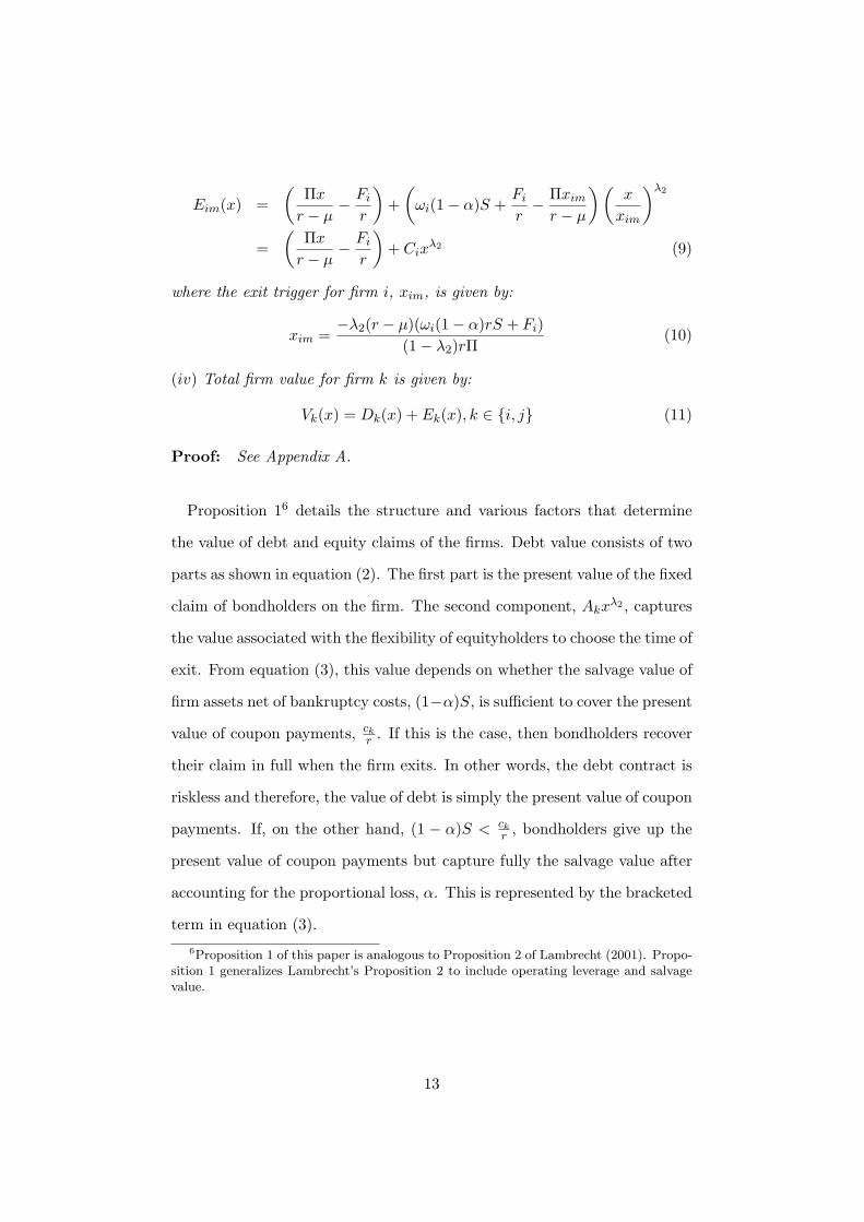
Vk(x) = Dk(x) + Ek(x), k ∈ i, j (11)

Proof: See Appendix A.

Proposition 16 details the structure and various factors that determine

the value of debt and equity claims of the firms. Debt value consists of two

parts as shown in equation (2). The first part is the present value of the fixed

claim of bondholders on the firm. The second component, Akxλ2 , captures

the value associated with the flexibility of equityholders to choose the time of

exit. From equation (3), this value depends on whether the salvage value of

firm assets net of bankruptcy costs, (1−α)S, is sufficient to cover the present

value of coupon payments, ckr. If this is the case, then bondholders recover

their claim in full when the firm exits. In other words, the debt contract is

riskless and therefore, the value of debt is simply the present value of coupon

payments. If, on the other hand, (1 − α)S < ckr, bondholders give up the

present value of coupon payments but capture fully the salvage value after

accounting for the proportional loss, α. This is represented by the bracketed

term in equation (3).

6Proposition 1 of this paper is analogous to Proposition 2 of Lambrecht (2001). Propo-sition 1 generalizes Lambrecht’s Proposition 2 to include operating leverage and salvagevalue.

13

As for the equity value, consider first firm j, which leaves the market

first. Its equity value is composed of three parts. First, the firm generates

operating revenues, πxt. The first term captures the present value of this

revenue stream discounted at the risk-adjusted rate. The firm must also pay

out the present value of fixed claims coming from financial and operating

leverage. This is captured by the second term. Together, these two parts

comprise the value of assets in place net of fixed obligations of the firm. The

final term in equation (4) characterizes the additional value associated with

the flexibility of equityholders to leave the market. Analogous to the debt

contract, at the exit trigger, xjd, equityholders give up the present value of

the assets in place and instead retrieve the salvage value of the assets.

The equity value of firm i comprises of two regions reflecting the product

market structure as shown in equation (7). In the region in which firm j has

not yet exited, firm i operates as duopolist. Therefore, its value comprises

the same elements as those in the equity value of firm j. The duopoly

equity value, however, is further enhanced by the strategic interaction. In

particular, the last term in equation (8) captures the incremental benefit

that accrues to firm i when firm j exits the market at xjd. Once firm j

leaves the market, firm i’s operating revenues jump by a factor Π

πand the

strategic effect disappears in equation (9), which captures the firm i value

as a monopolist.

The analysis in Proposition 1 is silent on which firm leaves the market

first. In what follows, I address this issue by considering various cases based

on relative strength of the firms. The analysis includes cases in which infor-

mation revelation occurs with strategic exercise of options as well as those

cases in which information revelation can break down. In the subsequent

14

analysis, the uninformed firm 1 is said to strictly dominate the informed

firm 2 of type k if F1 < Fk, k = L,H. Conversely, type k firm 2 strictly

dominates firm 1 if Fk < F1, k = L,H. In the case FL < F1 < FH , no

dominance occurs ex ante. Given these competitive environments, each firm

optimally determines when to exit the market based on its information set.

In particular, the uninformed firm 1 can choose to leave either at its duopoly

exit trigger, x1d or at the monopoly exit trigger x1m. The triggers x1d and

x1m are given, respectively by xjd and xim in Proposition 1 with the appro-

priate firm-specific parameters. Similarly, a type k firm 2 must determine

whether it exits at the duopoly trigger, xk2d or at the monopoly trigger, xk

2m.

Proposition 1 shows that all exit triggers are strictly increasing in the total

leverage of the firm. A higher firm leverage compared to the competitor,

therefore, implies that the firm exits the market sooner than the rival in

a frictionless environment. In terms of the information sets, knowing rival

firm leverage is equivalent to knowing the exit trigger.

Before analyzing these cases, it is crucial to define the concepts of reser-

vation trigger, which plays an important role in deriving the subsequent

equilibria, and revelation strategy.

As in Lambrecht (2001), the reservation trigger for firm i indicates how

long firm i would be willing to sustain losses if it could reap off monopoly

benefits once firm j exits the market. In order to define the reservation

trigger for firm i, consider Figure 1. Figure 1 shows the equity value of

firm i when it becomes the monopolist (the solid curve) and when it leaves

the market first at its duopoly exit trigger, xid (the dashed curve), denoted

by Ei(x) in equation (4) in Proposition 1. The U-shaped curves illustrate

the duopoly equity value of firm i, Eid(x) in equation (8), for different exit

15

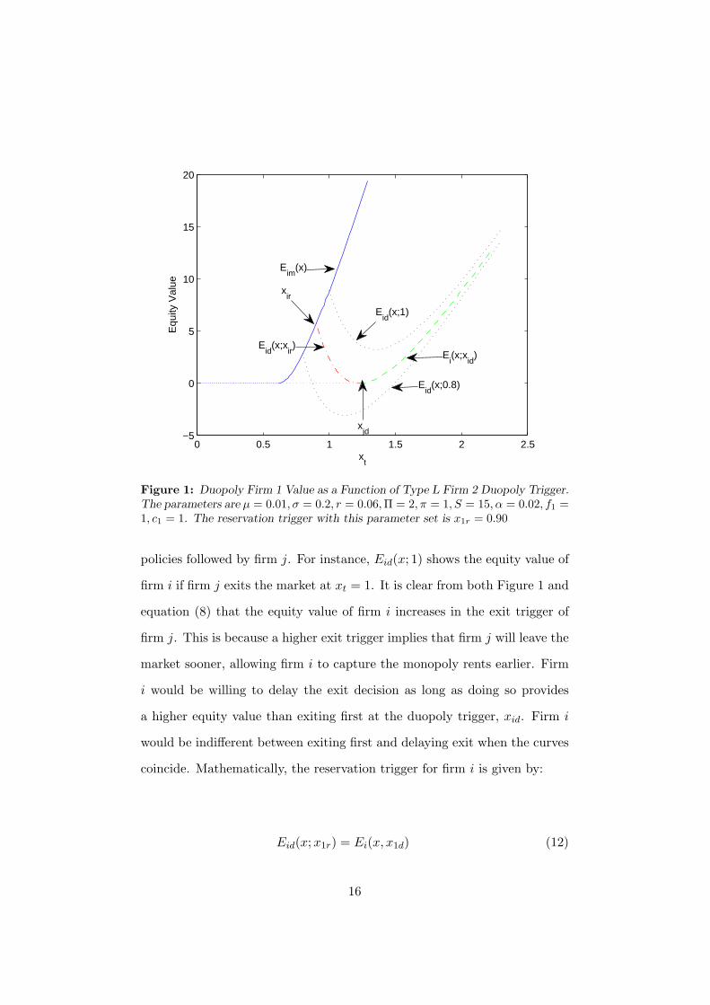
0 0.5 1 1.5 2 2.5−5

0

5

10

15

20

xt

Equ

ity V

alue

Eid

(x;1)

Eim

(x)

Eid

(x;0.8)

Ei(x;x

id)

xjd

xir

Eid

(x;xir)

Figure 1: Duopoly Firm 1 Value as a Function of Type L Firm 2 Duopoly Trigger.

The parameters are µ = 0.01, σ = 0.2, r = 0.06,Π = 2, π = 1, S = 15, α = 0.02, f1 =1, c1 = 1. The reservation trigger with this parameter set is x1r = 0.90

policies followed by firm j. For instance, Eid(x; 1) shows the equity value of

firm i if firm j exits the market at xt = 1. It is clear from both Figure 1 and

equation (8) that the equity value of firm i increases in the exit trigger of

firm j. This is because a higher exit trigger implies that firm j will leave the

market sooner, allowing firm i to capture the monopoly rents earlier. Firm

i would be willing to delay the exit decision as long as doing so provides

a higher equity value than exiting first at the duopoly trigger, xid. Firm i

would be indifferent between exiting first and delaying exit when the curves

coincide. Mathematically, the reservation trigger for firm i is given by:

Eid(x;x1r) = Ei(x, x1d) (12)

16

The left-hand-side of equation (12) indicates the equity value of firm i

when equity holders wait until the reservation trigger. The right-hand-side

of the equation captures the equity value when the firm exits the market

first at the duopoly trigger, xid. Applying equation (12) to firm 1 and type

k firm 2 yields the respective reservation tirggers:

x1r =

(ω1(1− α)rS + F1)(r − µ)

(Π− π)(1− λ2)r

(

1

xλ2

1d

−1

xλ2

1m

)1

1−λ2

xkr =

(ωk(1− α)rS + Fk)(r − µ)

(Π− π)(1− λ2)r

(

1

(xkd)λ2

−1

(xkm)λ2

)1

1−λ2

(13)

Note that the reservation trigger of each firm is a function only of its

own characteristics and market variables. In particular, the rival firm’s

characteristics such as its efficiency and financial leverage have no impact

on the reservation trigger. Furthermore, substituting for the exit triggers in

equation (12), it turns out that the reservation trigger is linearly increasing

in the firm’s total leverage. The reservation trigger can be written generically

as:

xir =(r − µ)

(1− λ2)r

[

πλ2 −Πλ2

(−λ2)λ2(Π− π)

]

1

1−λ2

(ωi(1− α)rS + Fi)

=(r − µ)

(1− λ2)rΩ(ωi(1− α)rS + Fi) (14)

Equation (14) allows us to make a natural order among reservation trig-

gers. This simplifies the derivation of the equilibrium. In addition, the reser-

vation trigger has the feature that it is between the duopoly and monopoly

thresholds, xim 6 xir 6 xid, i = 1, 2.

17

I now turn to the discussion of the revelation strategy. The revelation

strategy for the uninformed firm 1 aims to induce the rival firm to truth-

fully reveal its type through its actions. Since the action space for firm 2

involves exiting at either the duopoly or the monopoly triggers, the revela-

tion strategy leads a type H firm 2 to exit at xH2d, implying that the exercise

(or the lack thereof) of the exit option dissipates the information asymmetry

in the product markets. Note that firm 1 can devise a revelation strategy

using the reservation trigger. Since the reservation trigger measures a firm’s

willingness to endure losses in order to become a monopolist, a lower reser-

vation trigger can serve as a credible threat mechanism and force the H type

firm to truthfully reveal its type.

Having defined the concepts of the reservation trigger and the revelation

strategy, Proposition 2 establishes one of the main results of the paper in

the non-dominance case: that information revelation in product markets can

follow from strategic exercise of real options.

Proposition 2 (Information Revelation): Suppose FL < F1 < FH andx1d < xH

2r. Then the unique separating perfect Bayesian equilibrium (PBE)involves type L firm 2 leaving the market at its monopoly trigger and typeH firm 2 exiting when xt hits xH

2d. Firm 1 plays the revelation strategy inwhich it observes the firm 2 action at xH

2d. Firm 1 leaves the market eitherat its duopoly trigger if firm 2 has not exited at xH

2d or exits at the monopolytrigger if firm 2 has exited at xH

2d.

Proof: See Appendix A.

The significance of Proposition 2 stems from the fact that real options

exercises carry information. This information can be crucial so as to resolve

information asymmetry and to determine the outcome of product market

18

competition. Three remarks are in order here. First, although information

revelation ensures that the stronger firm in terms of total leverage outlives

the competitor, it does capture the possibility that the exit is due to high

debt rather than operating inefficiency. Suppose that firm 1 faces a type L

firm 2 and that f1 < fL. Firm 1 leaves the market due to relatively high

financial leverage if c1 − c2 > fL − f1.

Second, it is important to realize that Proposition 2 claims the separating

PBE is unique. The uniqueness of the PBE arises from the observation that

the firms play their dominant strategies given the parameter assumptions

in Proposition 2. In particular, a type H firm has no incentive to pool with

the type L firm since the duopoly trigger of firm 1 is below its reservation

trigger, xH2r. Hence, even if firm 1 is misled to believe that the competitor is

an L type firm, the exit at x1d would lead to unjustified losses beyond the

indifference point of the H type firm.

Finally, note that a full solution to the game describes what firms will do

for each possible parameter set, in particular, also when x1d ≥ xH2r. Following

the strategy outlined in Proposition 2 when x1d ≥ xH2r for the uninformed

firm 1 gives the high-leverage firm 2 the incentive to stay in the market

beyond its duopoly exit trigger. To see this, suppose that the state variable

hits xH2d. By staying until xH

2d − ǫ, ǫ > 0, the inefficient firm leads firm 1 to

believe that it faces a low-leverage rival and therefore, it leaves the market

at x1d. Since x1d ≥ xH2r, the high-leverage firm is willing to incur these

losses since it will eventually become a monopolist. Hence, the equilibrium

of Proposition 2 breaks down when x1d ≥ xH2r. On the other hand, since

the parameters of the game are known at the outset, firm 1 knows whether

or not x1d ≥ xH2r. The fact that the game is played in triggers implies firm

19

1 could devise another revelation strategy. If the expected payoff from the

revelation strategy is greater than that from exiting at the duopoly trigger,

firm 1 will adopt the revelation strategy. The revelation strategy when

x1d ≥ xH2r involves waiting until just after the reservation trigger of type H

firm 2, xH2r − ǫ. If firm 1 commits7 to this strategy, the best response of a

type H firm 2 would be to leave at the duopoly trigger. A type L firm 2

would wait until firm 1 leaves since xL2r < x1r. Note, however, that firm

1’s commitment to this strategy depends crucially on the beliefs it holds as

to the type of the rival upon observing no exit at the trigger xH2d. Denote

by r the conditional probability that firm 1 faces an L type rival given no

exit has occurred at xH2d. If firm 1 exits first at the duopoly trigger, its

expected equity value would be given by E1d(x) as specified in equation

(4). On the other hand, the revelation strategy yields an expected value

of rE1d(x;xH2r) + (1 − r)EH

1d(x). In this formulation, E1d(x;xH2r) denotes

the firm 1 value when equityholders exit at the reservation trigger of the

H type rival, xH2r, while EH

1d(x) is the value to equityholders when the rival

firm turns out to be an H type firm and exits at xH2d − ǫ, ǫ > 0. The latter

is given by equation (8). The next proposition shows that if the expected

value from the duopoly strategy exceeds that from the revelation strategy,

there exists indeed an equilibrium in which the high-leverage firm induces

the uninformed firm 1 to exit the market prematurely by taking advantage

of the information asymmetry.

Proposition 3: Suppose FL < F1 < FH and x1d ≥ xH2r. If firm 1’s prior

on an L type rival, p, satisfies

p ≥EH

1d(x)− E1d(x)

EH1d(x)− E1d(x;x

H2r)

(15)

7Firm 1 can credibly commit to the strategy since x1r < xH2r.

20

then there exists a PBE in which firm 1 leaves the market first at its duopolytrigger x1d.

Proof: See Appendix A.

Proposition 3 is another central result of the paper. For the result in

Proposition 3 to prevail, the uninformed firm’s prior about an L type rival

must be sufficiently high. When this is the case, firm 1 prefers to leave the

market first at its duopoly trigger. The distortionary effect of information

asymmetry may occur in a number of competitive settings and industry

characteristics. For instance, one may expect information asymmetry to be

particularly high in R&D intensive industries in which firms may want to

conceal private information in order to gain competitive advantage over the

rival. Information about a new entrant may also be scarce for an incumbent

firm.

The proposition shows a more efficient, low-debt firm can be driven out

of the market. In a sense, this result entails the evidence in Khanna and

Tice (2005) that a more efficient firm with high debt can be driven out of

the market earlier than a relatively less efficient rival with lower financial

leverage. At the same time, it is more general than the evidence in Khanna

and Tice (2005) since it shows that information asymmetry can cause the

exit of the stronger firm in the market.

Turning to the cases of strict dominance, Proposition 4 establishes that

as long as there is strict dominance between firms, information revelation

always takes place.

21

Proposition 4: (i) When F1 < Fk, k = L,H, the unique perfect Bayesianequilibrium involves firm 2 of type k = L,H leaving the market first. Typek firm equity value and the exit trigger are given by equations (4) and (5),respectively. The equity value of firm 1 is given by:

E1 =

pEL1d(x) + qEH

1d(x), if t < τHEL

1d(x), t ∈ [τH , τL]E1m(x), otherwise

(16)

where τk, k = L,H is the adapted stopping time at which type k firm 2 exits.Firm 1 exit trigger is as in equation (10).(ii) When Fk < F1, k = L,H, the unique perfect Bayesian equilibrium in-volves firm 2 of type k = L,H leaving the market last. Type k firm equityvalue and the exit trigger are given by equations (7) and (10), respectively.Firm 1 equity value and exit trigger are given by equations (4) and (5),respectively.

Proof: See Appendix A.

Similar to the previous results, Proposition 4 shows that total leverage

determines the order of exit in product markets. As opposed to Proposition

3, however, it argues that information asymmetry cannot be taken advantage

of and that it is immaterial to the outcome of competition. So long as there

is strict dominance between firms, the state variable and the exercise of

real options reveal private information. Similar to Proposition 2, the exit

in strict dominance cases might result either from operating inefficiency or

relatively high debt.

3 Economic Implications

This section aims to assess the significance of the results proposed in

Section 2 and to derive economic implications. Three broad questions are

addressed through simulations. First, how do firm values respond to changes

in crucial parameters of the model? Of particular interest is the effect of

information asymmetry on the value of the uninformed firm. Second, I

22

0 5 100

20

40

60

80

100

120

140

160

180

Demand Shock, xt

Tot

al F

irm 1

Val

uePanel A: Type L Rival

0 5 100

50

100

150

200

Demand Shock, xt

Tot

al F

irm 1

Val

ue

Panel B: Type H Rival

0 5 100

50

100

150

200

Demand Shock, xt

Tot

al F

irm 1

Val

ue

Panel C: Information Revelationp=1

p=0.2

p=0.5

p=0.5

p=0

p=1

p=1

p=0.5

p=0.2

x1m

xdH

xdL

xdH

xdH

x1d

Figure 2: Effect of Information Asymmetry on Uninformed Firm Value.

Panels A and B show the case F1 < Fk, k ∈ L,H. Panel C shows

information revelation conditional on type L rival.

investigate the relation between operating and financial leverage and analyze

corresponding empirical predictions. Finally, I define and show the risk

implications of the model. The parameter values used in the analysis are

given in Appendix B.

3.1 Implications for Firm Value

Figure 2 illustrates the impact of information asymmetry on the value

of the uninformed firm 1 for various values of the probability of an L type

rival. Panel A of Figure 2 conditions on an L type firm. The graph is

divided into four regions separated by the exit triggers x1m < xL2d < xH

2d.

The firm values are are identical in the regions in which xt < xH2d. This

is because all information asymmetry is resolved below xH2d. However, for

23

xt ≥ xH2d, the uninformed firm 1 value is an expectation over types. Several

observations are salient in Panel A. First, the figure exhibits a nonmonotonic

relation between firm value and the extent of information asymmetry. The

extent of information asymmetry is greatest at p = 0.5. Note that firm

value when p = 0.5 is between those when p = 1 and p = 0.2. Second,

when p = 1, that is, when firm 1 knows the rival’s type is L, firm 1 value

is continuous as shown by the dotted line in the figure. On the other hand,

when there is information asymmetry, firm 1 value jumps at the exit trigger

of an H type firm, xH2d. The size of the jump increases in the probability

of an H type firm, 1 − p. By attaching a higher probability to an H type

rival, firm 1 weighs the prospect of becoming a monopolist at an earlier

date, xH2d, relatively high. As firm 1 finds out that the rival is type L at

xH2d, the adjustment to firm value becomes more drastic. For instance, when

p = 0.5, the adjustment to firm value is about 11% whereas when p = 0.2,

the adjustment is as high as 22%. If one interprets p as the common prior

of firm 1 about the rival’s type, this observation shows the significance and

value of information held by competitors in product markets. Finally, note

that for large values of xt, the value functions close in on each other since, at

this range, firm 1 is far from the duopoly exit trigger xH2d and the probability

of becoming a monopolist soon is relatively low. The pattern of adjustment

is reversed when one conditions on an H type firm. Panel B of Figure 2

depicts this case. Analogous to Panel A, the graph is divided into three

regions separated by xH2d where information asymmetry is resolved and x1m

where firm 1 optimally leaves the market. In this case, p = 0 corresponds

to the perfect information setting in which firm 1 knows that the rival is

a highly leveraged firm. This is shown by long dashed lines in the figure.

When p = 0, firm 1 value is continuous. However, when there is information

24

asymmetry, firm 1 value experiences an upward adjustment at xH2d as it finds

out the rival’s type. This is because, before xH2d is hit, firm 1 value takes

into consideration the likelihood that the rival might be a low leveraged firm.

The value adjustment at xH2d is upward since the firm becomes a monopolist

at an earlier time relative to the case in which the rival is a low leveraged

firm. In other words, firm 1 receives either good or bad news when xH2d is

hit. In the case of Panel B, the news is good since the rival turns out to

be a high-leverage firm. As in Panel A, the adjustment to value in Panel

B is significant. When p = 0.5, the jump in value is approximately 13%.

A similar pattern is observed in Panel C of Figure 2 when F1 ∈ (FL, FH)

and x1d < xH2r so that the revelation strategy as outlined in Proposition 2

can be used. The figure conditions on the ex post realization of an L type

rival. The graph with the dashed lines shows the perfect information case

in which p = 1. In that case, firm 1 value is continuous and given simply

by its duopoly value without any strategic interaction terms.8 When there

is information asymmetry, firm 1 learns the rival’s type at xH2d = 2.90 and

firm value is adjusted accordingly. As with Panels A and B, the adjustment

at xH2d is significant.

3.2 Firm Leverage and Exit

The model developed in the paper defines firm leverage broadly as the

sum of financial leverage and operating leverage. Operating leverage, at the

same time, is the proxy for firm efficiency. In particular, it can be thought

of as a measure indicating how well the firm manages its supply chain and

networks or as a measure of production costs. Although all these relate to

real decisions of the firm as opposed to financial decisions, they represent a

8Refer to Proposition 1, equation (4).

25

fixed outlay for the firm as long as it operates. Therefore, it is analogous to

financial leverage.

In addition, operating leverage is often a consequence of the technology

choice of the firm. A change in technology can prove to be a difficult deci-

sion: it may involve a large, irreversible lump-sum investment cost as well

as adjustment costs and may require ongoing R&D activities prior to the

switch. Compared to a firm’s financial leverage, therefore, changes in oper-

ating leverage are more costly and likely to be infrequent.9 Recall also that

total firm leverage determines the competitive strength of the firm. That

is, firm i outlasts firm j so long as ci + fi = Fi < Fj = cj + fj . Therefore,

particularly in concentrated industries in which firms may have incentives

to induce the exit of their rivals, a firm’s financial leverage choice is con-

strained both by its technology choice and the leverage of its rivals. To see

this, suppose that fj < fi. If it turns out that cj − ci > fi − fj , a more

efficient firm will be driven out of the market due to excessive leverage since

Fi < Fj . Equivalently, for firm j to attain or maintain a competitive edge

over the rival, the portion of total leverage accounted for by debt, cj/Fj ,

must be bounded by Fi/Fj − fj/Fj .

Several testable implications emerge out of this. First, changes in a firm’s

technology and/or innovations that increase firm efficiency are expected to

precipitate a rise in financial leverage. Similarly, the financial leverage of

a firm is expected to increase subsequent to a major competitor’s exit or

contraction. This hypothesis is the result of two effects following a rival’s

exit. First, the firm’s financial leverage is no longer constrained by the

9This is not to say that changes in financial leverage can be carried out easily at nocost. See, among others, Fischer, Heinkel, and Zechner (1989) for a transaction-cost-basedexplanation.

26

rival firm’s leverage. Second, due to the exit of the rival, the firm can

experience an increase in its profitability, which, in turn, can lead to a

rise in financial leverage. At the industry level, the model predicts that

firms’ financial leverage moves together as increases (decreases) in the rival

firms’ debt relaxes (tightens) the constraint on other firms’ financial leverage,

ceteris paribus. Another policy implication is that firms with relatively high

debt levels are expected to invest more in measures that can increase firm

efficiency. This effect should be stronger in concentrated industries: as

Zingales (1998) and Khanna and Tice (2005) point out, in concentrated

industries with less levered rivals, predatory pricing can be observed. The

effect should also be observed more strongly for firms that are financially

constrained and unable to renegotiate the debt contract.

4 Conclusion

The empirical literature has shown the importance of the interaction be-

tween the capital structure choice and efficiency for a firm’s product market

behavior and the contraction and exit decisions. The evidence also suggests

that aggregate factors such as business cycles and industry features play

a crucial role as their impact differs across firms. This paper develops a

model that brings all these features together and analyzes the product mar-

ket competition with asymmetric information. The model illustrates how

firm-specific factors such as the debt, the efficiency and the quality of infor-

mation held about the rivals affect the exit decision in various competitive

environments. The relative position of a firm in terms of debt and efficiency

is an important determinant of the exit decision.

27

The model explains the role information asymmetry in the product mar-

kets. It shows that information asymmetry not only affects the outcome

of the product market competition but also contributes significantly to the

firm value and the risk dynamics. In particular, product market behavior

carries valuable information that can potentially change investors’ beliefs

about a firm’s future stream of cash flows.

Consistent with the empirical literature, the model predicts that a firm’s

total leverage is positively related to the probability of exit. The model dis-

tinguishes between the financial and the operating leverage. This distinction

allows one to link the exit decision explicitly to its drivers. Specifically, the

model shows that a relatively high level of debt can lead a firm to shut

down sooner. This result is consistent with the evidence in Khanna and

Tice (2005) and Zingales (1998). An important consequence of this result

is that the rival firms’ leverage imposes a constraint on a firm’s capital

structure choice. Furthermore, the model also generates a number of other

predictions. First, it predicts that the incumbent firms’ debt is expected to

increase following the exit or the contraction of the rival firms. Second, the

firms’ debt levels are expected to move together over time as the rival firms’

changes in their debt either tightens or relaxes the constraint on a firm’s

capital structure choice.

The model can be extended along several dimensions. A first step can

be to incorporate the product market pricing. In the reduced form model

of this paper, it is not clear how information asymmetry affects the pricing

decisions. Such an extension would also generate empirical predictions that

can be compared with the existing evidence in the literature. Second, the

model has the potential to investigate the impact of other firm-specific fea-

28

tures. Heterogeneous salvage values, for instance, would allow one to model

how the possibility of fire sales relate to the exit decisions. The model as-

sumes that a firm’s ability to control its costs is the proxy for its efficiency.

An alternative view of efficiency focuses on the firm’s ability to generate

cash flows from its asset base. Such alternative proxies can easily be in-

corporated into the model. Third, the distributional assumptions on the

information asymmetry can be relaxed or information asymmetry can be

assumed to be reciprocal. However, the qualitative results of the model are

unlikely to change as a consequence. Finally, the capital structure choice in

the model is a static decision of the firm. An interesting extension would be

to characterize the changes in capital structure and link it to the product

market competition.

Appendix

Appendix A. Proofs of Propositions

Proof of Proposition 1: To derive debt and equity values, I first valuea generic contingent claim, φ(x), that promises its holder a net cash flow ofg(x). Then I relate this value to debt and equity values.

Assuming complete markets, the no-arbitrage condition yields:

rφdt = gdt+ E(dφ) (17)

Using Ito’s lemma and taking expectations,

1

2σ2x2φ

′′

+ µxφ′

− rφ+ g = 0 (18)

The general solution to (18) is of the form:

φ(x) = A0 +A1xλ1 +A2x

λ2 (19)

where λ1 and λ2 are the roots of the following characteristic equation ob-

29

tained by plugging in the conjectured solution into the 18:

λ1 =1

2−

µ

σ2+

√

(

1

2−

µ

σ2

)2

+2r

σ2> 1

λ2 =1

2−

µ

σ2−

√

(

1

2−

µ

σ2

)2

+2r

σ2< 0

(20)

In equation (19), A0, A1 and A2 are constants to be determined from theboundary conditions.

To value debt, Dk(x), note that the debt contract promises a constantpayment of ckdt until the firm exits the market. Hence, g(x) = ck. To obtainthe coefficients in equation (19), impose the following boundary conditions:

limx→∞Dk(x) =ckr

Dk(xk) = min[(1− α)S, ckr]

(21)

where xk, k = i, j is the trigger at which equityholders leave the market.Note that this trigger is exogenous from the perspective of debtholders.The first of the boundary conditions tells that as xt tends to infinity, thevalue of debt approaches the present value of coupon payments discountedat the risk-free rate since for large xt, the probability of an eventual exitdiminishes. The second boundary condition regulates the behavior of debtvalue when the firm exits the market. Using these boundary conditionsyields the debt value in equations (2) and (3).

Before deriving equity value, it is useful to obtain an expression forthe portion of salvage value equityholders retain upon exit. The secondboundary condition in (21) indicates that if min[(1 − α)S, ck

r] = ck

r, then

the resale value of assets is sufficiently high so that equityholders retrievethe value (1 − α)S − ck

r, which, in turn, implies ωk(ck) = (1 − α) − ck

rS. If,

on the other hand, min[(1 − α)S, ckr] = (1 − α)S, then the salvage value

accrues to debtholders and equityholders receive nothing upon exit. In thiscase, ωk(ck) = 0.

Now consider the equity value of the firm that leaves the market first,firm j. In this case, g(x) = πx−Fj . To solve the differential in (18), imposethe following boundary conditions:

limx→∞Ej(x) =πx

r − µ−

Fj

rEj(xjd) = ωj(1− α)S∂Ej(xjd)

∂x= 0

(22)

The first of the boundary conditions is similar to that described for thedebt value. The second boundary condition is the so-called value-matching

30

condition which states that at the point of exit, equity value is simply equalto the salvage value recovered by equityholders. The third condition is thesmooth-pasting condition that ensures the optimality of the exit trigger.Solving equation (18) subject to the boundary conditions in (22) gives theequity value in (4) and the exit trigger in (5).

To derive Eid(x) in equation (8), impose the following boundary condi-tions:

limx→∞

Eid(x) =πx

r − µ−

Fi

r(23)

Eid(xjd) = Eim(xjd) (24)

Note that in equation (24), the duopoly equity value of firm i is partlydetermined by the action its rival takes. This is captured by the secondboundary condition. At xjd, firm j leaves the market, which entitles firmi to monopoly profits. Hence, the second boundary condition ensures thatequity value is continuous by equating Eid(x) to Eim(x) at xjd. After firmj has exited the market, firm i becomes a monopolist and its value satisfiesagain equation (18) with the following boundary conditions:

limx→∞

Eim(x) =Πx

r − µ−

Fi

r(25)

Eim(xim) = ωi(1− α)S (26)

∂Ei(xim)

∂x= 0 (27)

Solving equations (18), (24) and (27) delivers the third part of Proposition1.

Proof of Proposition 2: Before deriving the perfect Bayesian equilibrium(PBE), it is useful to describe the game in more detail. The game canbe modelled as a dynamic game of incomplete information in which theinformed firm 2 sends a signal to the uninformed firm 1 by either exiting orstaying in the market at the duopoly exit trigger of an H type firm, xH

2d. Inthe sequel, let M = m2L,m2H denote the set of signals sent by the typeL and type H firm 2, respectively. Hence, the set M = ne, e, for instance,corresponds to a setting in which a type L firm does not exit at xH

2d but antype H firm does.

Firm 1’s strategy space maps the signal sent by firm 2 to its action space.Let A = ane, ae denote the action taken by firm 1 upon observing no exit(ane) and exit (ae) at the duopoly trigger xH

2d. Once firm 1 observes rivalfirm behavior at xH

2d, it chooses whether to exit at its duopoly trigger, x1d,or the monopoly trigger, x1m.

The next step is to define the conditional probabilities firm 1 uses uponobserving firm 2’s signal. Let r denote the probability that the rival firm

31

is type L given that no exit has occurred at xH2d. Similarly, s denotes the

conditional probability of an L type rival when firm 2 exits at xH2d.

Let τH = inf

t : xt = xH2d

be an adapted stopping time denoting thetime at which the state variable first hits xH

2d. Consider the following strategyfor firm 1: (a) wait until xτH = xH

2d, (b) if at xτH = xH2d, firm 2 has not exited,

leave the market at x1d, (c) otherwise exit the market at x1m. In other words,firm 1 plays A = x1d, x1m. I now determine firms’ best responses to eachother under this scheme and argue that these best responses constitute thedominant strategies for each firm.

(1) First, consider type H firm 2. Since F1 < FH , by the strict mono-tonicity of the reservation triggers in the fixed costs, firm 1 can make acredible threat to type H firm 2 by holding on until x1r < xH

2r. Note alsothat type H firm 2 cannot mimic type L firm 2 since this requires that type Hfirm 2 wait credibly at least until x1d. But x1d < xH

2r by assumption. Hence,type H firm 2 would always leave the market at its duopoly trigger, xH

2d. Inother words, playing xH

2d is a dominant strategy for the H type firm.10

Now, consider type L firm 2. Since we have xL2r < x1r no matter what

strategy firm 1 follows, the best response of type L firm 2 would be to leavethe market at its monopoly trigger, xL

2m. Hence, exiting at xL2m is a dominant

strategy for a type L firm 2. Note that the ongoing discussion implies thetypes play a separating strategy and hence, r = 1 and s = 0.

(2) We now argue that the above profile outlined for firm 1 is the bestresponse to firm 2 strategies. Observe that for xt > xH

2d, firm 1 does notcommit itself to any strategy. Suppose now that xτH = xH

2d. Since regardlessof firm 1 strategy, type H(L) firm 2 will leave the market at its duopoly(monopoly) trigger, firm 1 finds out firm 2 type by observing firm 2 actionat xH

2d. If firm 2 has exited, firm 1 finds out that the competitor is of typeH and leaves the market at x1m by Proposition 1. If no exit has occurredat this point, firm 1 deduces that the competitor is of type L and thus exitsat x1d. Not only is x1d, x1m the best response to firm 2 strategies but itis also the dominant strategy for firm 1. To see why, note that if the rivalfirm exits at xH

2d, playing x1m dominates x1d by Proposition 1. If firm 2 hasnot exited at xH

2d, playing x1d dominates playing x1m since by assumptionx1d < xH

2r and only an L type firm would remain in the market for xt < xH2r.

In this case, since an L type firm plays its dominant strategy of xL2m, firm 1

would exit at x1d, ∀r ∈ [0, 1].Hence, the firms play their respective dominant strategies and the set

ne, e , x1d, x1m , r = 1, s = 0 constitute a PBE.

10It might happen that an H type firm trembles and does not leave at xH2d. But in

this case, the dominant strategy for the H type firm would be to leave the market atxH2d − ǫ, ǫ > 0.

32

Proof of Proposition 3: The structure of the game is similar to theone described for Proposition 2. Note, however, that although the signalspace remains the same as in Proposition 2, the action space for firm 1 nowdepends on the signal sent by firm 2. If firm 1 has observed exit at xHd , itsdecision is to choose whether to exit at x1d or at x1m. On the other hand,if firm 1 observes no exit behavior at xHd , it decides whether to exit whenxt hits x1d, or to wait until xHr in order to reveal rival firm type. As inProposition 2, however, if firm 2 exits at xH

2d, playing x1m is the dominantstrategy for firm 1. Therefore, in the sequel, I only consider firm 1 strategiesof the form ane, x1m.

Consider the case in which firm 2 has not exited at xH2d. We ask whether

there exists a belief, r, that justifies firm 1’s exit at the duopoly trigger x1d,thereby leading a type H firm 2 to become a monopolist.11

Consider the strategy x1d, x1m for firm 1. The expected payoff fromthis strategy is E1d(x) given in equation (4) since an L type rival would playits dominating strategy of leaving at xL

2m and an H type competitor wouldprefer to stay in the market beyond x1d since x1d ≥ xH

2r by assumption.Now consider the strategy

xH2r, x1m

. If firm 1 faces an L type rival,firm 2 would not exit at xH

2r and firm 1 would exit the market at xH2r as a

duopolist. Hence its value would be E1d(x;xH2r) where the value function is

as given in equation (4) but with the exit trigger x1d replaced with xH2r. On

the other hand, an H type rival would exit by xH2d− ǫ, ǫ > 0 to cut its losses.

This yields the value EH1d(x) given in equation (8). Hence, the expected

equity value from this strategy is:

rE1d(x;xH2r) + (1− r)EH

1d(x) (28)

Given the above expected values, firm 1 would perefer to leave at x1d ifE1d(x) is greater than the expression in (28). Manipulating this expressionthen yields:

r ≥EH

1d(x)− E1d(x)

EH1d(x)− E1d(x;x

H2r)

(29)

If firm 1 plays the above strategy, the best response of an L type firm2 is to play its dominant strategy of xL

2m while an H type firm plays xH2m

since xH2r ≤ x1d by assumption. This implies that firm 1’s updated beliefs

about an L type firm after observing no exit at xH2d, r, is given by the an-

terior probability p. Hence, the profile ne, ne , x1d, x1m , r = p wouldconstitute a pooling PBE if p satisfies equation (15).

11Recall that the working assumption is xH2r ≤ x1d. Therefore, it pays the H type firm

to hold on to the market until firm exits at x1d to capture monopoly rents.

33

Proof of Proposition 4: To prove part (i) of the proposition, distinguishbetween three cases depending on whether firm 2 types play separating orpooling strategies.(1) Suppose that both types play xkd, k = L,H, that is, both types exitat their respective duopoly triggers. Since x1m 6 x1r 6 x1d < xkd, k =L,H, firm 1 prefers to stay until its monopoly trigger. That is, exiting atthe monopoly trigger, x1m, is the best response of firm 1. This is easy tosee. Once firm 2 leaves the market at its duopoly trigger, firm 1 becomesthe monopolist. Proposition 1 shows that when firm 1 is a monopolist, itmaximizes its value if it waits until x1m. Now suppose that firm 1 indeedstays until x1m. As argued above, firm 2 would be willing to incur lossesuntil xkr to become a monopolist. However, by the strict monotonicity ofreservation triggers in the firm leverage, firm 1 can make a credible threatto firm 2 by holding on to the market until x1r. Given this, firm 2 wouldcut its losses and exit at the duopoly threshold. Hence the above profileconstitues a fixed point and is therefore an PBE.(2) Assume now that both types of firm 2 play xkm. It is evident that ifx1r < xkm and/or x1d < xkr , firm 2 would never play xkm, since firm 1 ineither case can hold on to the market longer than its competitor. However,even if x1m < xkr < x1d,

12 by the strict monotonicity of xir in Fi, we havex1r < xkr , k = L,H. That is, firm 1 can again hold out longer than firm 2to reap off monopoly profits. Hence, the best response of firm 1 is to stayuntil x1m. But since the best response of type k firm 2 is to exit at xkd, therecannot be any equilibrium with firm 1 leaving first when both types of firm2 play xkm.(3) It could also be that type L firm plays xL

2m and type H plays xH2d and

vice versa. However, the arguments in (2) establish that as long as x1r < xkr ,firm 1 can always outlast firm 2 no matter what type it is. Therefore, therecannot be any equilibrium involving firm 1 leaving first when types playseparating strategies.

It is straightforward to prove part (ii) of the proposition using the samearguments as in part (i). The proof again rests on the strict monotonicityof the reservation triggers in the fixed costs.

12That is, firm 2 could hold out until the duopoly trigger of firm 1 if it could becomethe monopolist.

34

Appendix B. Parameter Values

Table 1: Parameter Values for Figures 2-6

ParameterFigure 2

Figure 3 Figure 4 Figure 5 Figure 6Panel A&B Panel C

µ 0.01 0.01 -0.01 0.01 -0.01 0.01

σ 0.20 0.20 0.20 0.20 0.40 0.30

r 0.05 0.05 0.05 0.05 0.05 0.05

α 0.05 0.05 0.05 0.05 0.05 0.05

Π 2 2 2 2 5 5

π 1 1 1 1 1 1

S 20 20 20 20 20 20

f1 2 3.5 2 1 2 2

c1 2 2 4 1 3.5 5

fL 1.5 2 1 2 1 1

fH 2.5 3 2 4 2 3

c2 4 3 4 3 4 4

References

Bolton, P. and D. S. Scharfstein (1990). A theory of predation basedon agency problems in financial contracting. The American EconomicReview 80, 93–106.

Brander, J. A. and T. R. Lewis (1986). Oligopoly and financial structure:The limited liability effect. The American Economic Review 76, 956–970.

Chevalier, J. (1995). Do lbo supermarkets charge more? an empiricalanalysis of the effects of lbos on supermarket pricing. Journal of Fi-nance 50, 1095–1112.

Chevalier, J. and D. S. Scharfstein (1996). Capital market imperfectionsand countercyclical markups: Theory and evidence. American Eco-nomic Review 86, 703–725.

Dasgupta, S. and S. Titman (1998). Pricing strategy and financial policy.Review of Financial Studies 11, 705–737.

Fischer, E. O., R. Heinkel, and J. Zechner (1989). Dynamic capital struc-ture choice: Theory and tests. Journal of Finance 44, 19–40.

Fudenberg, D. and J. Tirole (1983). A theory of exit in duopoly. Econo-metrica 54, 943–960.

35

Ghemawat, P. and B. Nalebuff (1985). Exit. The Rand Journal of Eco-nomics 16, 184–194.

Grenadier, S. R. (1999). Information revelation through option exercise.The Review of Financial Studies 12, 95–129.

Khanna, N. and S. Tice (2005). Pricing, exit, and location decisions offirms: Evidence on the role of debt and operating efficiency. Journalof Financial Economics 75, 397–427.

Klemperer, P. (1995). Competition when consumers have switching costs:An overview with applications to industrial organization, macroeco-nomics, and international trade. Review of Economic Studies 62, 515–539.

Lambrecht, B. M. (2001). Impact of debt financing on entry and exit ina duopoly. The Review of Financial Studies 14, 765–804.

Lambrecht, B. M. and W. Perraudin (2003). Real options and preemptionunder incomplete information. Journal of Economic Dynamics andControl 27, 619–643.

Maksimovic, V. (1988). Capital structure in repeated oligopolies. TheRand Journal of Economics 19, 389–407.

Miltersen, K. R. and E. S. Schwartz (2007). Real Options with UncertainMaturity and Competition. Working Paper.

Murto, P. (2004). Exit in duopoly under uncertainty. The Rand Journalof Economics 35, 111–127.

Phillips, G. M. (1995). Increased debt and industry product markets: Anempirical analysis. Journal of Financial Economics 37, 189–238.

Phillips, G. M. and D. Kovenock (1997). Capital structure and productmarket behavior: An examination of plant exit and investment deci-sions. Review of Financial Studies 10, 767–803.

Poitevin, M. (1989). Financial signaling and the ”deep pocket” argument.The Rand Journal of Economics 2720, 26–40.

Zingales, L. (1998). Survival of the fittest or the fattest? exit and financingin the trucking industry. Journal of Finance 53, 905–938.

36