EhEEEEE - Defense Technical Information Center · 7d-r14i 091 applications of the variational...
98
7D-R14i 091 APPLICATIONS OF THE VARIATIONAL INTEGRAL IN ITERATIVE I I NUMERICAL SOLUTIONS..(U) AIR FORCE INST OF TECH I WRIGHT-PATTERSON RFB OH SCHOOL OFEENGI. K L MACDONALD pUNCLASSIFIED MAR 84 AFIT/GNE/ENP/84M-ii F/6 12/1 N EhEEEEE
Transcript of EhEEEEE - Defense Technical Information Center · 7d-r14i 091 applications of the variational...

7D-R14i 091 APPLICATIONS OF THE VARIATIONAL INTEGRAL IN ITERATIVE II NUMERICAL SOLUTIONS..(U) AIR FORCE INST OF TECHI WRIGHT-PATTERSON RFB OH SCHOOL OFEENGI. K L MACDONALD
pUNCLASSIFIED MAR 84 AFIT/GNE/ENP/84M-ii F/6 12/1 N
EhEEEEE

L3.
-:!--
-= 1-2W- L Ua L mUn
1=8
MICROCOPY RESOLUTION TEST CHARTNATIONAL BUREAU OF STANDARDS-1963-A
S.

7.r ~
Q6'S
NO
APLCTU FTEVRITOA NMqLI
ITRTV ERCLSU.OST ISTTIN YFe-EEIAIT"
I TI
W.5 MAY15S8
EPAT MET OF THEAI FRER Bl
AIRUIESIT
S ~- -I
Ap4 In MAY2 m 040 15 184

.4. ..o ..'° %
~~~ArIT IGIEWI 18 -- /
APPLICATIONS OF THE VARIATIOML IMEGRAL IN
ITERAIVE NMERICAL SOUITIO S TO THE
STATIONARY HEAT EQUATIOPS
THESIS
Ilark L. MacDonaldSecond Lieutenant, USAF
DTICl ELECTESAY 15 W84DJ
4 B
Approved for public release; distribution unlimited
le

4
AFIT/aNEIM/ I/4,-11
APPLICATIONS OF TC VARIATION AL ITT-7RAL
IN ITERATIVE I U ZRMICAL SOLUTIONS
TO T1 1
STATIARY HEAT EQUATIONS
TH1ESIS
Presented to the Faculty of the School of Engineering
of the Air Force Institute of Technology
Air University
in Partial Fulfillment of the
Requirements for the Degree of
IHaster of Science in Nuclear Engineering
iark L. icDonald, B.S.
Second Lieutenant, USAF
iiarch 1984
Approved for public release; distribution unlinited
.' ,,,:...:;.?, .,,..".::::...' ; . ....... ... .. ... , x~.... .. . . ...... ~ A~.....

A: Acknowledments
I would like to express my 4ppreciation to Dr. Bernard 1alan of
the Air Force Insitute of Technology for his I-uidance and assistance.
I would also like to thank Dr. N. Pagano of the Air Force IateriaIs
Laboratory for sponsoring this research project.
I-ark L. ilacDonald
ACCossiofn For
tNTIS C'~LTIC T't"
just 1 t
Dist specia l

Contents
4'4
Pace
Acl=owlederen ts ..................... ii
List of Figures . . . ............. . . ... v
List of Tables . . . . . . . . . . . . . . vii
Abstr ct .............. . ... viii
I. Introduction ........ ....... 1
Background . . . . . .1Problem . . . . . . . . ......... 2Scope *. . . ... .. .. .. 2Approach and Presentation . . . . . . . . . 2
II. Theoj * * . .. .. .... . . . .4. . . 4Variational Intezzral ... ........ 4Finite-Element 1.-ethod ....... .... 7Finite-Difference .ethod . . . . . . . o . . 9Solution of Simultaneous Equations . . . . . 11Stopping Criteria ............. 14
0III. Procedure . . . . . . . . . . . . . . . . . . . 22One-Dimensional Heat Equation . . . . . . . 22TNj-Dimensional Poisson Equation . . . . . . 26Two-Dimensional Laplace Equation . o . . . . 28Computer Codes ............... 31
IV. 1iurerical Results . . .. . . . . . .. . .. 34Variational Integral i irnirzn . . . . . . . . 34Stopping Criteria ............. 41Accuracy Criterion .. .. .. . . . .... 54
V. Conclusions and Recamendations .. - . o . . . . 59Conclusions . . . . . . . . . . . . . . .. 59Recootjndations .............. 60
Bibliograhy .. . . ............ 61
Appendix A: Exact Variational Integral . . . . . . . 53
i i
* . t. yI% -- a

Appendix E: Finite-Flemant Derivation for the 1-Dheat Ecuation ... . . . . . . . . . . . 65
Ap )pendix C: Derivation of an Anai! tical Solution for?oizson's Equation . . . . . . . . . . . . . . G9
Appendi.:: D: Scooppirx Criteria .............. 74
Vita . . . . . . . . . . 0 . . . . . C4
S. iv
- . , -'Of*-..-

List of Ficures
2.1 iiesh for a Retar-a Region 11...........
2.2 Iteration Limit . . . . . . . . . . . . . 16
2.3 y.otetical Iteration Lmit Comparison ...... 20
3.1 Heat Conduction in a Thin Rod . . . . . . . . 22
3.2 ibdal Divisions for the Thin Rod ........... . . . 24
3.3 Matrix Equation for Finite-Difference Approximation,Four Nodes . . . . . . . . . . . . . . . . . . . . . 25
3.4 Finite-Element Arrangement (Case One) . . . . . . . 29
* 3.5 Finite-Element Arrangement (Case To) . . . . . . . 30
4.1 Variational Integral iininin, 1-D Problem, FourNodes . . . . ..a . . .. .. .. . . . .. .. 35
4.2 Variational Integral I1inum, I-D Problem, EiitNodes . . . . . . . . . . .. 36
4.3 Variational Integral Ianimuzz, 1-D Problem, Sixteen-T odes . . . . . 0. . . . . . . . . . . . . . 37
4.4 Variational Integral H1inim~m,, Poisson Problem,Four ! odes o. . . .. . . . ......... . 38
4.5 Variational Integral dininx, Laplace Problem,Four Nodes . . . . . .. . . . . . . . .. .. 39
4.6 Temperature and Variational Integral Convergence . . 42
4.7 Stoppinw Criterion Comparison . . o o . . . . . . . 43
4 4.8 Error 1iorn Approximation .............. 45
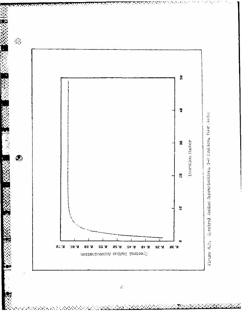
4.9 Spectral Padius Approximation, 1-D Problem, FourH odes *. .. . . .. .. .. .. .. . . .. . 46
4.10 Spectral Radius Approximation, 1-D Problem, Ei htNodes . . . . . . . . . . . . . . .. . . . . . . 47
V

Figure ke
4.11 Spectral Radius Approximation, 1-1 Problem, SixteenNodes ........ . . . . . ....... . 45
4.12 Nodal Tem'perature Suni . .............. . 49
4.13 Variational Integral ................ ....... 51
4.14 Stopping Criterion, Initial Trial Solution Abovethe Exact Solution ............. . . .. 52
4.15 Stopping Criterion, Initial Trial Solution belowthe Exact Solution . o . . . . . . . . . . . . . . . 53
4.16 Schematic Illustration of Accuracy CriterionFailure . .. .. .. .. .. ... .. .... 57
B.1 Finite-Zlement Temperature Interpolations . . . . . 65
D.1 Stopping Criterion, 1-D Problem, Four iodes .... 75
D.2 Stopping Criterion, 1-D Problem, Eight 1odes . . . . 76
D.3 Stopping Criterion, 1-D Problem, Sixteen Nodes . . . 77
D.4 Stopping Criterion, Poisson Problem, 4 x 4lo e . . . . . • . . . .• . . . . . .• . . . . 73
D.5 Stopping Criterion, Poisson Problem, 6 6% Nodes .. .. .. .. .. ... . . .... 79
" D.6 Stopoing Criterion, Poisson Problem, 5:: 8
14odes . . . . . . . . . . . . . . . . . . . . . . 60
D.7 Stopping Criterion, Laplace Problem, 4 x 4Nodes-l . .. . . . . . . . . . . . . . . .
D.8 Stopping Criterion, Laplace Problem, 6 x 6
D.9 Stopping Criterion, Laplace Problem, 8 0
Nodes • .. . . . •. . . 83
Svi
AL'.O

List of Tables
Table Page
I Variational Integral Approximation ........ .40
II Integral and Error Iorm Linima ....... ... 54
III Integral and Error i br for 1-D Problem ...... .55
IV Nodal Temperatures for 1-D Problem (Four lbdes) . . 56
V Integral and Error Non for Poisson Problem .. .... 58
vii
JII
. vii
9

Th-ree stationary heat cuations or solvec,- usinj- thie finite-p
di-fference n,,er-hoi. Thei ros-Fultin- set of are'aceiuations .. r
solve-- usin- the -auso-Seidcl iterative tecchfl.-ue. The ternoerazur'as
atC thc nodal n..ointz- .-ere su1)stituteci into a irricr'icz1 an)oro.:ination ofJ
the variationa. integral. The variational inte.-ral apr:iation wa-Cs
used to determine iwhlen to stos -the ite-rative process. The- war'iatioia
int~zrl soD~ri~crieror. %ras coprdto a stoprsin: criterion that
uses the dis-ilacenent be-t-.'e en iterations to arxiat te error
*bevvween. the iterative solution and the exact" solution. T.-he variational
intce-ral vias fo-..nd to be less effective as a stoni-in- criterion than
th,,e error esti,:.ate.
The variational integ,:ral wa xnndas a -. e-thod of determining,
whater thie finite-difference technrdiue or thie firnite-ele:.ent technmicue
--ave a mrore accurate solution. It ,.-as found t.hat the variational' in-
tc_:ral failecd, in some- cases, to rrcit the r..rozU'r-at '- t a
,.V
vii

. . .
I Introduction
Backciround
In practice, the number of boundary value problems that can be
solved analytically is quite limited. Consequently, numerical techni-
ques are used to approximate the partial differential equations associ-
ated with the boundary value problems. These nunrical techniques
often lead to large sets of simultaneous equations. These ec _1'.ins
are usually sparse (they contain few non-zero elements in thc oeffi-
cient matrix).
Iterative techniques are often used to solve large sets of simul-
taneous equations. These techniques have two major advantages over
methods that solve the simultaneous equations directly. First, itera-
Live methods avoid calculations with the many zero elements in the
coefficient matrix while direct methods perform calculations on every
element of the coefficient matrix. Secondly, iterative methods are not
as susceptible to the accumulation of round-off error.
An important difficulty with the iterative techniques is
determining when a sufficient number of iterations has been corpleted
to ensure an accurate solution. This thesis addresses the problem of
when to stop iterating.
1ny boundary value problems can be expressed as variational
integrals to be minimized. Accordingly, one possible test for conver-
gence oi the numerical solution to the boundary value problem is
whether it minimizes the associated variational integral.
--..#
• %I . --P- - . .- -- . - - . -..- -.- - - - - . , - ',.'. .,4". . -. ,.- -.. : .-.. . - ° '..
.1J4
Problem
The prinary purpose of this thesis is to determine the usefulness
of the variational integral as a test for termtinating the iterative
process.
The secondary purpose is to determine the usefulness of the
variational integral as a neans of determining %-ich numerical miethod
gives a more accurate solution.
Tbis thesis is limited to the study of stationary (time-inde-
pendent) heat equations in one and two spacial din-es ions. The numeri-
cal approximations to the boundary value problems consist of the
tinite-difference and finite-elennt techniaues. The iterative scheme
used is the Gauss-Seidel method (mitehod of successive displacements).
Approach and Presentation
* Section Ii introduces the theory necessary to understand the
variational integral, the finite-difference n'othod, and the finite-
elerptnt method. The Gauss-Seidel iterative technique is discussed.
The concept of norms is introduced and is applied in exan'r-imcg stopping
criteria.
Section III introduces the three stationary heat equations con-
sidered in this thesis. The variational integral formlations of the
prblenis are given and the numerical approximation techniques are
applied.
% Section IV presents the results of the study. First, errors
caused by approximating the variational integral are examined. Next,
the utility of the variational integral as a stopping criterion is
2

discussed. Finally, the usefulness of the variational integral as a
means of determining which numerical method gives a more accurate
solution is analyzed.
Section V drawrs conclusions and gives recamendations for future
studies.
.'.
-I.'Is
3
q0 . . . *~ . .*- .v * - " . . . . " " . . . " " q "% i . ."

V
Variationa 1 limtgra.
M.any problems in the physical sciences can be solved in two ways.
First, they can be written as differential equations subject to given
boundary conditions. Secondly, they can be written as variational
integrals to be extremized (maximized or m~inimized). The two formunla-
tions are equivalent because the function that will extremize the
variational integral will also satisfy the differential equation. This
equivalence ia demonstrated by the fact that the variational integral
is extremized only when an equation, called the Dler-lagrange
*, equation, is satisfied. This Euler-Lagrange equation is precisely the4 " same as the differential equation formulation of the problem
(Ref 8:67). In general, only elliptic differential equations can be
written in variational form (Refs 8:117; 5:164) but same exceptions
have been found (Ref 7:252-256).
In variational calculus, one looks for the function t(x,y) with
*' continuous second partial derivatives, that extremizes I (t) on region R
of the x-y plane:
1(M f!RF(x,y,t,t x t )dxdy (2.1)
where
t = t(x,y) (2.2)
,t (X Y)
ty= f Ix,y) (2.3)
t = t t(x, y) (2.4)y Cy
A' 4

-'T find t (x,y), examine the set of functions
t(x,y) = t(x,y) + En (x,y) (2.5)
where £ takes on some value close to zero and Th(x,y) is an arbitrary
function with continuous second partial derivatives. At this point, an
inportant assumption is made. It is assumed that t is given on the
boundary as a constant or as a function of x and y. As a consequence,
t is rot subject to variation on the boundary and i(x,y) nust equal
zero on the boundary.
Substituting Eq (2.5) into Eq (2.1) gives
J(s:) - I(t+En) = ffRF(X,y,t+Cr,tx+sn ,t +cn )dxdy (2.6)R X xy y
A necessary condition for I to nave an extremLun at t t is that
J(s) must have an extreum at E = 0. So
(E) IE= = 0 (2.7)
Differentiating Eq (2.6) with respect to c gives
~~3 ;;.ts(C) = R a " + Dx + @, DE d--%y (2.8)
or
= 1 = ss + rJ + r, -- W d (2.9)
By the chain rule (Ref 1:92)
at / F)=;F + a (2.10)axw;x t:3xa

| ..
Il
, Vtherefore
DF a, 3F r) a13'(.11
k =a 7- rvW T- (2.11
and
_ 3_ (r4 )- n -) (2.12)
Substituting Eqs (2.11) and (2.12) into Eq (2.9) gives
[ 3F D 3 ~3 F(C t - F - F dxd
+ a DF ) ,_Fd3 (2.13)
By applying Green's Theoren (Ref 1:197), the second integral in Eq
(12.13) can be transformed into a line integral
[F _L a xdFffjm ai ax Ah ay at yJ
@I( - t dxF (2.14)
But since n (x,y) = l e boundary, C
aJ(C) =ffn1i--- I-(-- idxy (2.15)
60*

Recall that
- (a ) 0 (2.7)
3Crh E0=O
if I is to have an extre mz at t = t. Therefore
[F_ a ( Wa F aF xdy 0 (2.16)
Since n is an arbitrary function of x and y then
aF a /3F = /3F (2.17)
Eq (2.17) is the Euler-Lagrange equation and it nust be satisfied for t
to extremize I(t). In the derivation that lead to Eq (2.17), it was
assumed that the function, t, was specified on the boundaries (Dirich-
let boundary conditions). Other boundary conditions could produce a
change in the integral that is to be extremized. A method of determining
the variational integral for other boundary conditions is given in
Mlikhlin (Ref 12:116-121). For all the problems considered in this
thesis, the Eler-Lagrange equation given as Eq (2.17) will give us a
function, F that extremizes I(t) as given in Eq (2.1).
Finite-Elemient 1-kathod
The finite eleuent method involves extremizing the variational
formulation of the problem. The solution region is divided into
interconnected subdmaiuns - the finite elenents. The elements in
one-dimensional problems are line segments. The Irost versatile ele-
ments in higher dimaisions are triangles for two-dimensional problems
4nd tetrahedrons for three-dimensional problem (&ef 8:86). Next,
iterpolation functions are chosen to represent the tenperatures
7
"".." "

over each element. These interpolation iunctions are often poly-
nanials. Suppose the function being integrated under the variational
-, integral contains derivatives up to the (r+l)th order. Then, the
v$.i interpolation tunctions must have rth order continuous derivatives at
the element interfaces and (r+l)th order continuous derivatives within
each element (Ref 8:124). When these criteria are met, the variational
integral for the entire solution region can be written as the sum of
the variational integrals of each element (Ref 8:78).
An interpolation function for the teeratures on an element is
written in terms of the nodal values associated with that element. The
variational integral is evaluated over the element and the integral is
differentiated with respect to the nodes and set equal to zero in order
to extremize the variational integral on that element. The equations
for each element are assembled to give the equations governing the
temperature over the entire region. in this mamer, a set of equations
is created which can be solved simultaneously to find the temperatures
at the element nodes. This set of sinmul=aneous equations can be
written in matrix form
At = b (2.18)
whkere
A = a coefficient matrix
t = vector of unknown nodal temperatures
b = vector of knwn constantsA
Rather than go into the details of the process here, an eample is
given in Appendix A.
8
A%

Finite-Difference Method
A differential equation can be converted into finite-difference
torm by approixmating the derivatives in the equation by dffferences.
The elementary definition of a derivative is (Ref 3:54)
dt lim t(x + x) - t(x) (219)dx -xO Ax
The derivative is approximated by a divided difference
dt z t(x + Ax) - t(x) (2.20)Ux Ax
In ne-dimensional problems, the solution region is broken into
line segments and a nodal point and its neighboring nodal points are
used to approximte the derivative at that nodal point. In this
manner, a linear difference equation is created for each nodal point.
The equations for the individual nodal points can be assembled to give
a set of algebraic equations to be solved simultaneously. Linear
combinations of Taylor series expansions give several difference
*, formulas with their associated truncation error (Ref 3:55-59):
First forward difference
4 .i6[=dt t(x + h) - t(x) + O(h) (2.21)
First central difference
dt t(x + h) - t(x - h) + o(h 2 (2.22)
S(.22h
j .1A9
99

-I.
. First backward difference
dt t(x) - t(x - h) + 0(h) (2.23)
Second forward difference
d2t - t(x + 2h) - 2t(x + h) + t(x) + O(h) (2.24)
dx2 h2
Second central difference
d 2.t - t(x + h) -2t(x) + t(x -h) + 0(h 2 ) (2.25)
dx2 h2
Second backward difference
A -t(x) - 2t(x - h) + t(x - 2h) + 0h (2.26)
dx2 h2
* where h is the distance between nodal points. Truncation error is a
result of ignoring higher order terms in the Taylor series. The
finite-difference method is also subject to scmthing called round-off
error. Round-off error is the result of the tact that a corputer can
store a limited number of significant figures. The total error due to
both trmcation and round-off error will be referred to as the discreti-
*zation error. It is the difference between the analytical solution and
the finite-difference solution at a particular nodal point.
For two-dimensional problems, a rectangular mesh is imposed over
the solution region in order to find approximate temperatures at the
nodal point of the mesh.
10
V-V V -".9, ~ ~ j~

.J ,1-b ,. , , , . ,- ,2 -,,' .,,7 _ ". .. -1 -j_ .-" . ' , " ' - , .,. . . .. .
-7-i
x
Figure 2. 1. Mesh for a Rectangular Region
Solution of Simultaneous Equations
Both the finite-elenent and finite-difference methods lead to a
set of simultaneous liner algebraic equations. There are two methods
of solving for the unknowns in these equations -- direct methods and
indirect methods. Direct methods lead to an exact answer, excluding
round-off error, after a finite number of arithmetic operations.
Direct methods tend to be time consuming since each element in the
coefficient matrix must be operated upon. In general, N3 operations
are required where N is the number of equations (Refs 3:111; 5:209).
Sae examples of exact methods are Gaussian Elimination and the lhcamis
method (Ref 3:9-12; 44-48).
Indirect iterative methods require an infinite number of opera-
tions to solve the equations exactly, but an adequate solution can
11

usually be achieved in a finite number of steps. These methods usually
require less than N3 operations, especially if there are many zeros in
the coefficient matrix as is the case in the finite-elenent and finite-
difference equations. Furthermore, cunulative round-off error does not
grow as in the direct methods (Ret 3:111).
The matrix equation
At = b (2.18)
can be re-written
t = Gt + c (2.27)
An iterative solution can be written in the form
4. (n+l) = Gt(n ) + c (2.28)
where
t(n ) = nth iterated vector
G = iteration matrix
c = known constant vector
The three most carrmnly used iteration methods are the Jacobi,
Gauss-Seidel, and successive over-relaxation rethods. They are derived
by factoring the coefficient matrix into strictly upper triangular,
diagonol and lower triangular matricies denoted by U, D, and L respec-
tively (Ref 3:46-47):
(U + D + L)t = b (2.29)
The Gauss-Seidel ithod (also known as the irethod of successive
displace nts) is used in this thesis. It expresses the (n+l)th
12

iterative vector in terms of both the nth iterative vector elkients and
the (n+l)th iterative vector elements as soon as they beccni available:(n"1 (n)
(L +D)t (n + l ) = -Ut -n ) + b (2.30)
or written in a fom similar to Ecj (2.27)
(n+1) -n)t = -(L + D)-Ut' n ) + (L + D) b (2.31)
Translated into a ccmputational algorithm:
(i-iz (n+l) n (n)_n(l)l1
t i a.-E a..t. + Z ai.t j -b (2.32)aii j=la jt j=i+l
where aij is the element in the ith raw and the jth column of the
coefficient matrix. One begins the process by choosing some arbitrary
initial trial vector, t 10 ) .
Norms
in the following sections, we will be concerned with measuring the
difference between exact temperatures aerived analytically and the
tenperatures found fra the iterative process. The error vector is
defined as
e (n) = t - t(n) (2.33)
where
e (n) = the error vector for the nth iteration
t = vector of exact nodal temperatures
t(n) = vector of nodal temperatures fran the nth iteration
rhe displacement vector (also known as the "residual vector") is
defined as
13
}" "' d (n) tl(n+l) t (n)G-34,. = - (2.34)
where
t (nk+l) = vector of nodal temperatures frat. the (n+l)th iteration
t (n) = vector of temperatures fram the nth iteration
It is often more convenient to measure the size of these vectors
as scalar quantities. A nom, symbolized by I I I , will allow one to
do just that. A vector n-norm can be defined by
I ItI In = (:ItiIn)1/n (2.35)1
where
t = vector
t. = ith element of vector t4I. 1
()The norm used in this thesis is
11tI = .tl. (2.36)
Stopping Criteria
Standard Method. One of the fundairental difficulties with itera-
tive methods is detenining when to stop iterating. Som common
criteria are (Ref 4:227)
I t ( ) _ t ( n- 1 ) I 1( . 7
or
or (n) -t (n-1)
. 4i t(n) < E (2.38)
for some prescribed c or
1
;; .. v ....,,'M, ,'J~~iv .'<.q,,- ...''< .. . .. " .. "" -'. ..14":.

n >N (2.39)
for some given N.
The problen with the above criteria is that
it(n) _ n-) < C (2.37)
.des not imply that
Ht(n - ti < E (2.40)
Figure 2.2 illustrates this fact (Ref 9:5). Thus, for problems where
convergence is slow, t ( may be far from the exact tenperature even
though it would have eventually been reached. However, choosing an
iteration limit that is to stringent might lead to a considerable waste
of ccmputer time.
A simple technique has been found that will allow one to use the
displacement vector, I d(n) II to estimate the error, IIe(n) i (Ref 14).
Recall that the matrix ecuation can be written as
t = Gt + c (2.27)
And an iterative solution can be written as
t(n+ l) = Gt (n ) + c (2.28)
%.
" 1y subtract Eq (2.28) fran Eq (2.27), the error vector can be written
e (n+l ) = Ge(n) (2.41)
.... The following discussion holds for all real srmmetric and scme
real nonsymmetric matricies (Ref 3:27). Assume that the initial error
5.%
5.0
'', ,... . '1 -. -*% . . -. , - ,, , - . , ". . .•.- , '. ' ' '. " . - " ". "..** "° -. - . , .. - - , '1

2; t (0)
iteration limit
errorTrue V. V _
Tenrp.
_ _ _ I _ __ _
Iteration n1,xer
Figure 2.2. Iteration Limit.
vector can be expanded in terms of eigenvectors Vi of the iteration
matrix G (Ref 14:236)
(0) iIC V . (2.42)
wbere C are scalars and m is the dineision of the square coefficientVl
matrix. Frcn Eq (2.4 1)
e (n ) = Oe 1(0 ) (2.43)
where Gn is G raised to the nth power.
16
V.V
,!d, 1J L ?.,.. , .

a77
: :'." e~~n) =_ n ZCV.(.4
In)
e ) = C.G'V. (2.45)
i=l 3- -;-
But GV. = X.V. by the definition of an eigenvalue where X. is an-1 1-1-a
eigenvalue corresponding to V ThenInl
e (n ) E _Cixinv i (2.46)i7-1
-- = 12 n .+( Xm n
e n ) ( n+ ... C(V (2.47)
If A1 1 > !x2 1 > Ix 31 > .. > 1Xm1
then for large sufficiently large n
e (n) X 1 nCIll (2.48)
e (n + l ) > 1ln+lcIVI (2.49)
so
e(n+l) > 1e(n) (2.50)
• .In order for the error vector to vanish
I x1 <1 (2.51)
IX_1 is called the spectral radius. Dq (2.50) shc;s that if 1 is
mnall, convergence occurs rapidly. In general, X1 increases for a
larger number of unknowns (Ref 3:116; 16:87). Thus, a problem takes
more iterations to solve as one increases the number of nodal points
., :.. used in the finite-difference and finite-elerent methods.
17

- - a - . . , . . . .. . . -
Fran Eq (2.33)
t t tn) + e( n ) (2.52)
"A. and fro=. Eq (2.50)
t t(n+l) + i e (n ) (2.53)
el.u~n.nating e (n ) between Eq (2.52) and Eq (2.53) gives
t t (n + l ) _ i t (n )
z (2.54)* .. 1
-a
- or t (n + l ) _ ( n )
t z t + tn - - (2.55)
Fran Eq (2.55), it can be seen that, if X. is close to one, then small
differences between successive iterations does not inply that the
iterative solution is close to the exact solution. But, given the
definition of the error vector and the displacement vector, the error
vector can be approximated by
(n) d(n)e -- (2.56)
a- "or-p..
:;.? 1Id(n) IlIle In) -I 1 (2.57)
'5l
18

.. 7.7 '7..
For most problens A will not be known but can be approximated in
the following manner (Ref 14:241). For sufficiently large n
e n) (n-1) (2.58)
1-•e"- (n+l) _e(n) (e(n) -e (n-1) (.9
t :(t n + l ) - t (n ) (t (l tn ) - t (n - i ) ( 2.60)
od n ) X Al (n-1)
(2.61)
(n)
1ii d -(2.62)I d_1 (
Therefore
"d(n)II
S~1 d(n)~ (2.63)( ( )
. One now has a sinple means of estimating the error between the
true solution and the iterative solution at the nth iteration and,
therefore, a criterion for stopping the iterative process. The
variational integral will be judged against this criterion. Young
provides a more refined version of this error approximation stopping
criterion (Ref 17:226-227). Warren gives a more detailed analysis of
this and related error estimates (Met 16).
Variational Integral. Since the variational integral is
ext-remzed for the exact solution to the boundary value problem, it is
.19

thought that the nodal temperatures frun the iterativc riethod can be
4 substituted into a numerical approximation of the variat-ional integral.
As the nodal temperatures approach the exact values at the nodal
points, the variational integral should be extremize. Thus, an error
criterion might be
"\" f~n ) llnl~l -(2.64)
for sane prescribed E. This criterion might not have the difficulty
that the standard criteria had for slowly converging problems as
illustrated in Figure 2.3.
V ...:
Va~riational1
Integr'al
I terationS Diffe'ren-ce
7 (rI+i)
I aIteration -Differece Zt ( n+l )
'%Ieain Itl_
Figure 2.3. Hypothetical Iteration Lit Comparison
20

.. .. , It is also thought that the variational integral can be used as a
stopping criteria for a special case of problems where the temperatures
,rom the iterative technique are either mstly above or mostly belcw
the exact values. Suppose the initial trial solution for nodal tepera-
tures is above the exact values but the iterative rrethod converges to
temperatures below the exact values; then, at some iteration, the
iterative solution will pass through the exact solution and the varia-
tional integral will be extremized. In practice, one will not kncw the
exact values but an initial trial solution can be chosen that is known
to be above the true solution and then an initial trial solution can be
chosen that is known to be below the true solution. One of these trial
solutions will pass through the exact solution.
v.
"-
21"'.

III Procedure
In this section, the three heat equatlons used in this thesis qnd
the computer codes used to evaluate the problnes are exaraned.
One-Dimensional Heat Equation
The problem to be examined is shown in Figure 3.1. The equation
to be solved is
d 2 t 2t = 0 (3.1)dx2
where m is a constant. The boundary conditions are
t (0) =1 (3.2)
d () 0(3.3)
141%
i t =1 thir rodI --- 0dx
L
Figure 3.1. Heat Conduction in a Thin Rod.
22

%4........ .......... ......... .......... ......... ..... 7. T . 17 7. -.q, 1 N .N .w -. . . . . . . . " , . :"
The equation is easily solved (Ref 11:21):
.t - cosh[m(L - x). (3.4),....Cos-, (mL)-
Variational Integrai. The variational integral for the
one-dimensional heat equation can be developed by ccmparing the
governing differential equation (Eq (3.1)) with the Euler-Lagrange
* equation in one dimension:
D.4 -F _d ( F 0 (3.5)
xI
The result of the comparison is that
.. 7 M (36
0 Thus, the integral to be extremized can be written
I(t) = 1 L , m2t d (3.7)
In order to use the variational integral when only the nodal
temperatures are known, the derivative in Eq (3.7) is approximated by a
forward difference and the integral is appro.imated by a sum (Ref
10:235):
%-t
ti+l ii(t) i+l -ti) + mti2 (xi+1 -x i) (3.8)
one can use the botuxary condition given in 14 (3.3) and the forward
difference approximation given by Eq (2.21) to show that for i = N,
23

tN% %- (3.9)
For the purpose of validating the computer code, the variational
v . integral was solved analytically in Appendix A:A.
1(t) = tanh(mL) (3.10)
Finite-Difference Fonrmlation. The thin rod shown in Figure 3.1
is divided with a number of equally spaced nodes as shown in Figure 3._ .
1 2 L- 1 T+- C.
4-.;
Figure 3.2. Nodal Divisions for Thin Rod.
The differential equation is approximated using Eq (2.25):
t i+ -2t i + ti I 2h2 + = 0 (3.11)
24
,-- .. . . . . . . ., .. . . ., . . .4 . . . . . , . . . . .. , , , ,, , .. , .. . . .. . . . . . -, -.+,,- .. " .. . . . . .. ,,- . . . .,. . . - . . .- . . . . . . . . . . . . . . . . . . ... . . " .'

-- W ..-.-.
where
h =xi+ -x i (3.12)
Eq 1(3.11) can also be written as
-ti_ + Dti - t4 = 0 (3.13)
where
D = 2 + (mhL) 2 (3.14)
Using the boundary condition given as Eq (3.3) and the central
difference approximation given by Eq (2.22),
• ,(, t+l= t- 1 (3.15)
thus Eq (3.13) for i = N is given by
-2t 1 _1 + DtIN - 0 (3.16)
and using the boundary condition given as Eq (3.2)
Dt t= 1 (3.17)
Therefore, for a problem with four unknown nodal temperatures, the
simultaneous equations can be written in matrix form as shown in Figure
3.3.D -1 0 0 tI 1-1 D -1 0 t 0
0 -1 D -1 t 3 0
,L% 0 0 -2 D t 4 L0
Figure 3.3. Matxix Equation for Finite-Difference Approximation, Four
.odes.25

% -"4 .,..
In order to validate the caputer cxde, m = 2 and L 1 so
that the tenperatures could be ccrpared with those given in the
literature (Wef 11:243).
Finite-Eienent Formulation. Tht. iite-elenent irethod is inore
involved than the finite-difference method and the derivation of the
matrix equation is given in Appendix B. The matrix fonulation of the
problem turns out to be identical to the finite-difference fornilation
(Figure 3.3) except that
", D = 12 + 4(mhL)2 (3.18)6 - (mhL)
oTwo-Dimensional Poisson's Equation
The problem to be examined is a square plate with uniform energy
generation across the plate. The equation to be solved is
-2t 2t + 0(3.19)2 2 k
-4..ax @y
where g and k are constants. The boundary conditions are
-(0,y)= 0 (3.20)
9t.WI(x,0) = 0 (3.21)
t(L,y) = 0 (3.22)
t(x,L) = 0 (3.23)
, . ..,, ',,2
i . 26

(-..
[ q The analytic solution is rather involved and is Qeveloped in Appendix
"":C. For the validation purposes, g, k, and L were set equal to one so
Sthat the numerical solutions could be camare with the literature lef
. Ii:260,384).
Variational integral. The variation~al integral is de'veloped by
-[i comparing the differential equation with the Euler-Lagrange equation in
<. two dimensions (Eq 2.17)). Thne integral is given by
ii1 I2t = I(LR ) 2- _-c
(dx[Lt)dy (3.25)
Theintegral is approximated by sums over both the x and y directions.
Thbe derivatives are approximated by back-wards differences in order to
take advantage of the derivative boundary conditions in the same way
~that the forward difference was used to take advantage of the deriva-
t4 ive boundary codto nthe one-dinvensional problem (pg. 23):
4.
' 1N M (ti"j - t i-l,j2
It 2i=0 j=0 A
.'. Ay i'jj 39xVy (3.26)
-j., ein addinat tional iitegral was solved analytically for
cFputer co e validation. oe derivation is very similar to the
derivation for the one-dimeensioul problem given in Appendix A.
ccm"Finite-Difference Formulation. The sqare plate is overlayed by a
system of square meshes each of dimension h by h.
27
',
. ''. .' 'C '.- . L -. .' :. -""" . '-"" ."""" 2 . (-" ". 2 '""" """". . " " " ' " 1 •" "-"- .

The heat equation Eq (3.19)) can be approximated using Eq (2.25):
-1 (ti+l,j -2tj +ti-l, ) +j+l 2ti, + t + 0 (3.27)
...%
where
x = ih (3.28)
y = jh (3.29)
The subscripts must be combined before the function, t, can be repre-
sented by a vector. This is easily done by incremnting the subscript
j through its range of values while, for each j, incrementing i through
its range of values. A matrix equation is found for the two-dimensional
problem in a manner very similar to -.hat of the one-dimensional problem
fdiscussed on page 24.
Finite-Element Fornulation. Triangular elements are used in the
two-dimensional problem. If one uses the same nodal points as used in
the finite-difference scheme, then the elements can be oriented in two
different fashions. The orientation in Figure 3.4 will be referred to
as "Case One" and the orientation in Figure 3.5 will be referred to as
"Case Two." The two arrangements lead to different matrix equations
and, consequently, different solutions.<' ,.TWo-Dimensional Laplace' s Equation
The problem to be considered is a square plate
a2t +at 0 (3.30)x2 + y2 =
28

subet to the boundary, conditions (.1
t (0,y) 0 03.32
t~x,L) =0 (3.33)
-t * (L,v) =101) (3.34)
y
-. .
%a.
Fiue3..FnteEam, r.geet(as n)
, *29

"-% .'.
x
Figure 3.5. Finite-Elewent Arrangement (Case IUV).
The problem is a rather starndard boundary value problem. There rore,
the analytic solution will not be derived i this thesis. Thne solution~r
Js given by (PEf 6:107):
00 200(1 - cos (nrr)) sinh (nx)sin ( ) (335)
t XY)=nl n-,sinh (nT-) LL(.5
Variational Integral. -lie variational integral is developed by
ccraring the differential equation with the L'uler-Lagrarige equation.
The integral is given by
I Mt2 + M 2 xy(3.36)
30
- . .-.. .. . . .. .. .. .
".%" % ,

.*,u -.' , . -f - _ - ' . " . . a -. -. - . -'
"'aV
The integral is approxirlated by sums over both the x and y directions.
Tne derivations are approximated by central dfferences."-"
N M .- t. 2 t(t) 1 ~ ~ i-l, t + i,j+l - t i'j-i h2
--t). "+ 2h h (3.37). It)z i=0 j=0 2h 2h
Finite-Difference Formlation. ,he square plate is overlayed by a
system of square Meshes and the problem is solved in the same way as
the Poisson problem. Due to tire constraints, the problem was not
solved using finite-elenent techniques.
Ccuputer Codes
All codes were written in Fortran-77 for a DEC Vax 11/780 ccputer.The cCUputer programs were quite similar for all three heat equations.
For each of the boundary value problems, a program was developed
that calculated the exact temperatures at the nodes and then varied
these temperatures by a given percentage. These tenperatures were
substituted into the variational integral approximation to determine
what effect errors in the temperatures had on the value of the varia-
tionzil integral.
Another code was written for each problem that was used in the
* zaalysis of the variational integral as a stopping criterion and as an
accuracy criterion. The matrix Lquations from the finite-difference
aria finite-element methods were solved iteratively using the Gauss-
Seidel mthod. The exact solution at the nodal points was calculated
using the analytical solution. After each iteration, the difference
ap d
31
-. . aa

between the exact and iterative temperatures was used to calculate the
percent difference between the exact and approximate temperatures
- [ (n)[ = [I - t (n) HII!.( - , ___ i_(3.38)
The difference between successive iterations was used to calculate
the percent change in temperature
I a")I t (n) - (3.39).4.
(n)_ t -
The reason for these new relationships is that when one actually
uses a stopping criteria, the percent error in a solution is usually
more useful than the absolute error. This also allows a ccparison
between the standard stopping criterion and the variational integral
criterion by eliminating the magnitudes of the temperatures and varia-
tional integrals. Note that Eqs (3.38) and (3.39) are very similar to
the error vector and displacement vector previously defined. In the
following sections the terms "error nori" and "displacement norm" will
*, refer to Eqs (3.38) and (3.39). The relationship
() -= f(n) (3.40)
?'_;;:,[ [ ! (n-)
is assumed to hold although it cannot be rigorously developed as was Eq
(2.63).
432
*..' 32
* .:,. ::.- :.'c

. .' The variational integral was cmpiuted after each iteration by
substituting the temperatures frm the iterative process into the
varidtional integral approximation. To ccaipare the variational inte-
gral as a stopping criterion to the stopping criterion defined in Eq
(3.40), the percent change in the variational integral is defined as
"£': l(n) _ (n-l)l
IAI(n) ' = (3.41)
.;3
.I*I* .9 .. . . . . . . . . . . . ., . , , - . . . . + . . . . . . . . . . . . . . . . . + . . .' a ., . ° " 4 " " ' - " , ' , °
" " " " " ' " " " " " " " " " "
" ...
" " " . . ' "
IV Numerical Results
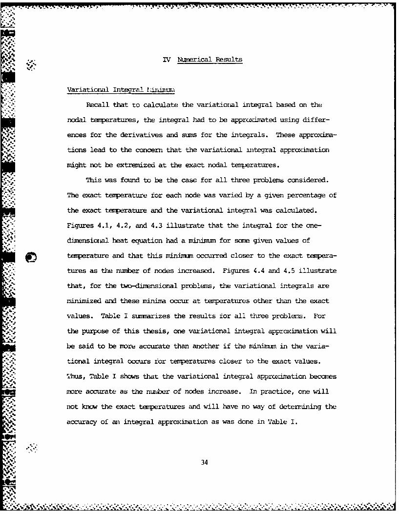
Variational Integra! I rLmci.r
Recall that to calculate the variational integral based on the
nodal tenTeratures, the integral had to be approximated using differ-
4ences for the derivatives and sums for the integrals. These approxima-
tions lead to the concern that the variational ntegral approximation
might not be extremized at the exact nodal teneratures.
This was found to be the case for all three problems considered.
... The exact temperature for each node was varied by a given percentage of
the exact temperature and the variational integral was calculated.
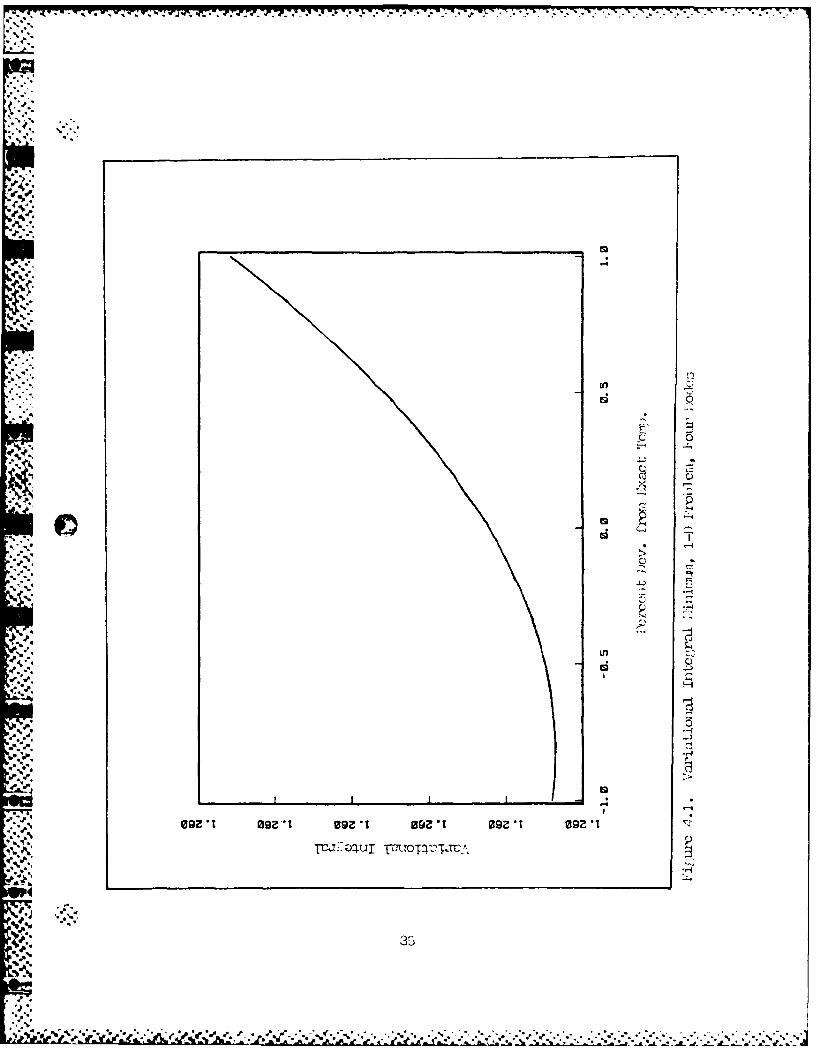
Figures 4.1, 4.2, and 4.3 illustrate that the integral for the one-
dimensiol heat equation had a minir=u for some given values of
Atemperature and that this =mnu occurred closer to the exact tempera-
.- tures as the number of nodes increased. Figures 4.4 and 4.5 illustrate
that, for the tWo-dixensional problems, the variational integrals are
minimized and these minima occur at temperatures other than the exact
values. Table I summarizes the results ±or all three problems. Forthe purpose of this thesis, one variational integral approximation will
be said to be more accurate than another if the ndnimum in the varia-
4.'-t tional integral occurs for temperatures closer to the exact values.
Thus, Table I shows that the variational integral approxiation becames
more accurate as the nutiber of nodes increase. In practice, one will
not know the exact temperatures and will have no way of determining the-4
accuracy of an integral approxination as was done in Table I.
:34
(4..
'4..V..* 9s.*
I'...
~ 4.
V.p4...
4h. %*.1~
In C.
0
E0
0,..
4..? 22
'4. *444%4
4,, 04.. .1~)
4~4. -.% -~ o
:..
4... U,V.
4..)V4 4-.* H
'.4 5-4
-4. 4-.
~~4~4~~~** -4
.4
6
-4 4-4
*444
ggVt 09Z1 0~.t 09~T 09VT~7o~uI r~1'3TdT~A
"4'.~ .~..
3S
.4
* 4,~

-. p.
9-:
o-
• e'
.:
4 .° • - • - _
.. ......... :- ... ' .. ' . ' .....- . :.;.v :.. : . .: : 2-,: ,) ' ;_U

C4
.4-.4
4.3 7

~. .~*,
.* .~
S. -~
-- 4: *~-~
-. 9.
-S*5%~
2
9: *5..* o4..) r4
*% *5'** x -
.5-S-S ~q
r -
S L.~
- 4*. -4S . '9
.9.,- 1 '-S* ** -S/ -S
C)
5- -4I C) -.
U') -"
Sd C)-I-,% '-Se
.4..9..
.5..4*5* *55*
* -4.5-
-a *. (-.5
'4 ~J~OU) uOtVt~TJ~A
-4.5.4
~
.4
9. 9. 5, -. * .. '. .% * - '9.9:9:9:9:9:9:9. *~-S~*~5*5.5% *5,** --- S * *** .* -S * - .5 5....--. - .55~5.S S S -- "-S u-SS*55 S *~.* S5*t*.~ ***,~*. *.*.*.*.*.

.1* .
* II
a..'.
,p. I •
_ * )
,--1
5. ii I IC
uu St uee £LE 0
5:,-
**• % * - . - . . - - - -. - - - ° .. . .- . .,- . -- , . -o -. -. . -o. - .- , . .. . -".'. ° -. -. .' ° "

.7
The exact value of the variational integral is calculated using
the analytical solution as shown in Appendix A. It can be seen, in
Table I, that the value of the variational integral approximation does
not approach the value of the exact variational integral in the Poisson
problem even though the accuracy of the integral approximation improves
for an increasing number of nodes (using the definition of accuracy
given above). Thus, relating the value of the integral approximation
to the exact value is of little use. Furthermre, one will not be able
to calculate the exact variational integral in "real-wdorld" problems
since the analytic solution will not be known.
Table I
Variational Integral Approximation
PoeExact Integral Percent. ""Problem Integral 1 Nodes Approximation 2 Deviation 3
4 1.260 -0.80One-Dimen. 0.964 8 1.105 -0.21
16 1.033 -0.0532 0.993 -0.01
Two-Dimen. 4x4 -0.1070 +13Poisson -0.1406 6x6 -0.0947 +9
8x8 -0.0884 +7
D.-Dimen. 4x4 4.35xi03 -53Laplace 1.04x10⁴ 6x6 5.92xi0 -45
8x8 7.21x10³ -39
1. Value of variational integral using analytic solution.
2. Value of variational integral approximation at its minimum.
3. Percent deviation from exact nodal temperatures where theminimun in the variational integral occurs.
40
. . . . . . .

,- . . .
Stopping Criteria
Recall fron Section II, that for a problemi with slow convergence,
the difference between tenperatures for successive iterations coula be
snall even though the difference between the iterated value and the
exact value was still quite large. t was thought that the variational
integral might give an alternative evaluation for terination since the
integral is extrtnized as the iterated nodal teperatures approach the
exact nodal temperatures. Figure 4.6 shows that as the stun of the
iterated temperatures approaches the sum of the exact temperatures, the
variational integral converges to a constant value.
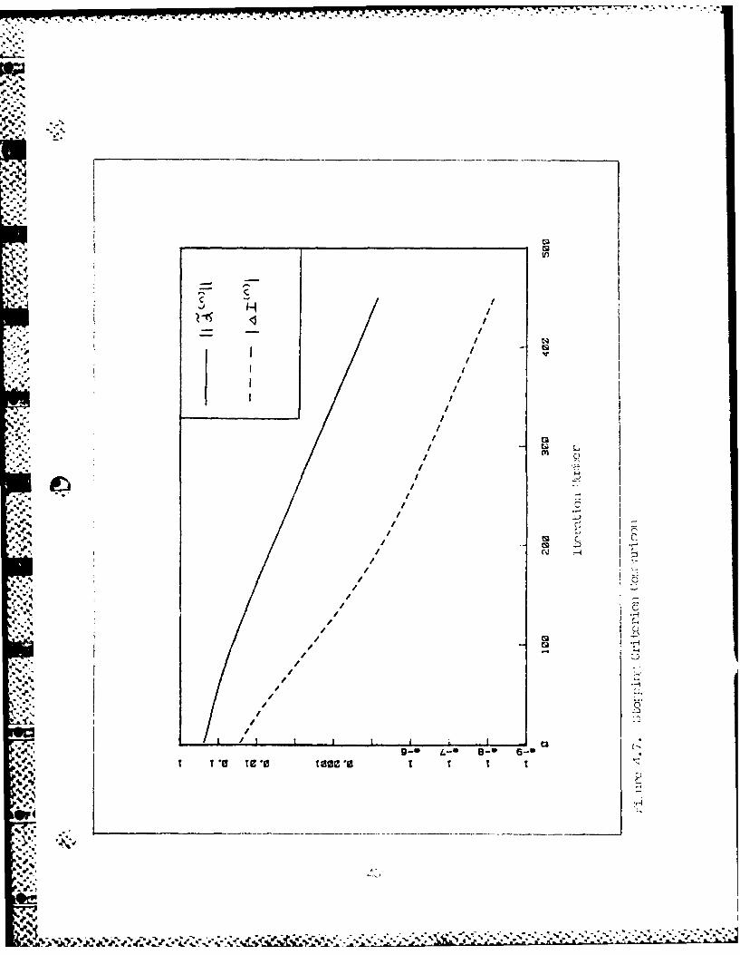
Figure 4.7 compares a common stopping criterion, IldlnII with the
variational integral stopping criterion, ! (n) It can be seen from
Figure 4.7 that, past a certain iteration, dn) 1 and (n)
* decrease at the same rate.
One can easily explain the linear decrease in [dn I (keeping in
A . mind nhat the y-axis in Figure 4.7 is a logarithmic scale). The slope
of ,, (n),, is given by
M = logl!a~n) {- _log! a(n-ll'j (4.1)
n - (n-i)
Recall that for large n
w.. .. I j{a (n ) }
SxI1 =(4.2)aj (n-1) H
or
logIA 1 - log, fa(n) II- log!ld(n-)fJl (4.3)
41
oil° - -. 5 .- ... * .S* . . * . .
* ° . . ........ * . *. * *0*

.5
II
'..- i °.
.n ' . I
* -I ,1
* II
* ," - I
I : I' ..
.%
" 4- ">]!-
:'.4% ,,' 4..4%;
""c: I " "
/ -
4.. * I
4 : t . / c
• O
.. * / ,.
4%.' /
II
1 / l_ I I/. i -4[
9_% 4." O- -
. o.. -- ,
Ii 43+ ^
"+ +I . /
' '+ ,", h!: +,,.., .'.+,,t +,-% +,"+ . .. ,. .,v .,, : " :: -. .. . ,, . -C-., ..- -. -., .,. -. . - +, . . . " .". ,+.",- ,,- .4 r ., .. - . .. .. . -." +,- ,,",ii.% -,.. .- . . -.- ,. . -. ". . . . +, - - .,, .

-.. . . . - - --
J-." .. By comparison of Lq. (4.1) and (4.3), it can be seen that
m = logi (4.4)
l.re importantly, Figure 4.7 shows that for sufficiently large n
! i Ixl In) (4.5);
.- ~-~-~'-~-- *' -~ -' - -. -' -£
4.
F
-V..
-% -~ .j1
-I
I C
'I
/I /
I I/
/I
I //
/I
/ .
* ~ 1~ . ~
//
/
/c~ C)~ -wN I-I
N'.
a
I,--4
I (4* I
r 0 ~0 1000'i. % t
C,)
Py4
'/ .y.P~P ..
4.
44.
*4%~
in
aea
d6I*0 91 0 *0 Ss*0 0; 0 ir*0 v 0 E 1 K *
Wl)

- --.- ~ -- - - - . - - . . - - - . -
V.'4
(4~
________ UU
.4.
U C)U,
p., -
k2
"4
4p -C) C)*~~44 -~
-4
U -~
Q-r
4-' '-4
C).4 4-' 0I -4
I 4-'.44
-- I
.4.
'-4.4.
UIn
.1
44,
4 -pC.)
NU
0t 0'8 0'-4
.4.44~4 N
uo~:Txo.Iodv v1r~tr: m~;~a~:
2U
-. 4
1"-'
'4-
*4%
.*.**.**~*.*.*~.**.. ~ .q* ~ -. -~ *~ .4 .4 44 ~*** .4~* .4 r4~* \~444~* ** .4 .4 ~1a *4~ *--* - -4 449*4 - A...

" ,:1
(4,l
h'.\p'. in
4'.2
4%%p

h. ,
, -I
e "
V I
I , I-i..
!III.qII

1.
the iterative method Passing through the sum of the exact nodal tuer-
atures after tlirty-seven iterations. Thus, one would expect the
variational integral to be extrernzed at the thirty-seventh iteration.
Ficure 4.13 shows that the variational integral was actually minimized
after ineteen iterations. This is understandable in light of the
S. previous discussion in which it was found that the variational integral
approximation is minimized for temperatures other than the exact
values. The results frm Figures 4.12 and 4.13 can be represented more
concisely using fAI (n) and I , (n) I . Figure 4.14 shows that the
variational integral stopping criterion, AI(n), has a "cusp" or local
minuinm where the variational integral is a minimum (nineteenth itera-
tion) and the error norm, jje(n) I has a cusp where the iterative
solution passes through the exact solution (thirty-seventh iteration).
In Figure 4.14, the initial trial solution was greater than the exact
solution. The finite-difference equations converged to temperatures
below the exact values. Figure 4.15 shows that when the initial trial
solution was below the exact solution, the iterative temperatures did
not pass through the exact values and no cusps were observed for either
IAI (n) I or 116(n) 1. Table II ccapares the iteration number where the
integral apprximatior is minimized to the iteration number where the
error norm is minimized. Appendix D shows that the results of the
stopping criteria study hold for all three problenils and all nodal
densities considered.
50
*4°

,L U,
.-. :.-
in
...- J
4
"°'-4
'
iU I . **I* . '! . -

* ...-.
C -
~q) ~ /- I -I I I/I,'
o
* I0 /
____________________________ //
/
III
I - -
4 1
.w4 / .
I - -
I/4 / 0
I-iI
I
'I C)
5, J
I
- c~j
00! - - - - - - - - - ~jj~* .5-4
* &4.)
I
I - I I I I I
0! 70 T90 t00*0 100000 I
C-.
%** **%*
*~"-h '
.5.
~~5f~*1

*, m .. - i
/°" I
• ~/ -
/ I-.
I 2"D
I
//
/ "
I --- .
%,Iw
-I I1 II8" 0 " ggg"
t/
/ lI'
" ,", ... ... . -.. . . .. , " ,, . . .. . , . ,. . . ' " - . . . .- . ... . .., .. . . ., . ,,..I. .. . .K.

Table II
Integral and Ehror Norm Minima
I2Probleml Nodes Integral2
4 6 96 15 26
One-Dimen. 8 30 5310 51 9016 150 280
qxw-Diren. 4x4 20 38
Poisson 6x6 43 968x9 74 185
Two-Dimien. 4x4 7 32Laplace 6x6 18 66
8x8 35 ill
1. Using the finite-difference method
2. Iteration number where the minimnm occurs
Accuracy Criterion
Since the variational integral is mindmized for the exact solu-
tion, it was thought that the variational integral approximation
could be used to determine which numerical method would give the best
approximation to the true solution. Two methods were considered--the
finite diffenxce method and the finite-element, method. Due to tine
constraints, only the one-divensional problem and the Poisson problem
were considered. Table III shows the results for the one-dimensional
problem.
,5lI,.

W f _ t f .* ~ ~ 7 ~ W ~~ . * ._ -~ ~ ' ~. *. K .r , o 7-
ft ft
,-...Integral and F-ror Norm for 1-D Problem
t.'.Nodes FPthod 1ntegr,
SFD 1.3720 0.0759..- F 1.3695 0.0812
,- .4 FD 1. 2606 0. 0549FE 1. 2594 0. 0569
5 - FD 1. 1967 0. 0429.FE !. 1960 0.0436
"--.6 FD 1. 1553 0. 0351- FE 1. 1.550 0. 0352
'- 7 FD 1.1264 0. 0298,'.> FE 1. 1262 0. 0295
, FD 1.1051 0.0259FE 1.3049 0.0253
4 FD: Finite-Dffere1nce MethodFE: Finite-E!erwent Method
,[ .:<Note that for nodal densities of less than six, the tenmperatures
, ! from the f inite-ele nt method rminimze the variational integral even
m though the finite-difference mthod minimizes the error norm. Ikxdal
[.[. -dusities greater than eight were considered but they gave the same
" -""results as densities six through eight and, consequently, were not
..... ;._. included in the table. The discrepancy between the integral and error
. .- _ norm for nodal densities less than six" cwi be explained. Table IV
• . '-' shows that the temeatures for the finite-elenent method are less than
$, the exact tenperatures while the tenperatures from the finite-dif-
'.-'4" .. -. ference method are greater than the exact terperatures.- f55
:E:1.550:.035
° 7 l 116o009FE".1620.29

Table I7V
Nodal Temperatures for .-D rrobln (Four Nodes)
Node Exact Finite-Diff. Finite-Elem.
1 0.6252 0.6289 0.62152 0.4102 0.4150 0.40513 0.2998 0.3049 0.29434 0.2658 0.2710 0.2604
Figure 4.16 is based on Figures 4.1 through 4.5 and shows how the
variational integral could fail to predict which rethod is most accu-
rate. For nodal densities greater than or equal to six, the finite-
element mthod gives more accurate temperatures and, therefore, the
variational integral approxiimtion correctly predicts the more accurate
ethod.
The results for the Poisson problem are sinTarized in Table V. It
4A was found that one finite-element case gave the rost accurate tempera-
tures while the other finite-element case gave the least accurate
answers. For all nodal densities considered, the variational integral
correctly predicted which rethod gave the most accurate solution. The
difficulty that occurred in the one-dimensional problem did not occur
for the Poisson problem because the majority of teoperatures for all
three methods gave tenperatures below the exact values.
56

. - . -
.~% *.~
I C...A 4-4
Q-4-,
+N
_____ C) --- 4
"N2 6
I.:
0
'-4
C)
.' ~% I -) IV.. I -
6* .*4~. ,-4
-. 4 -~
r4N.
C)
-1-,
0
.9
U)- a.
* .4* -4%
I~3 ~~1
4.. V 'if V-.' %'%~iV. *~*.'* **->*.. ~.$/.** - ., -2- *2-VW.-. ~-. -. ~-K - :-. *~*&*.~ 2 -V.A

=.*.
Table \7
Integral and Error Norm for Ibisson Problem
1Nodes Method ntegral HFE-2 -0.1632 0.4147
2x2 FD -0.1.680 0.1891FE-I -0.1710 0.0844
FE-2 -0.1806 0.39664x4 FD -0.1815 0.2143
FE-I -0.1821 0.1024
FE-2 -0.1940 0.39618x8 FD -0.1942 0.2366
4 FE-I -0.1944 0.1223
1. FD: Finite-Difference MethodFE-I: Finite-Elenent Method (Case COne)FE-2: Finite-Eement Method (Case Tklo)
_.5
A.!'p!
U*,.,. ". . - -"".- - - """ ... " '' -' " ' ," " '- - -" " . - .['' " , z , . . . , -,. '' "5 -' ,L .i.

*, , ,,,. i..- -. .,, *., , ., , . ., -,. '- . - . . . . . .. . .. . . ... . . . . .. . .. .
Conclusions and Reccaendations
""Conclusions
The variational integral approximation for each of the three
boundary value problems was minimized for temperatures other thun the
exact values. As the number of nodes was increased, the approximations
W*re nimiunzed at temperatures closer to the exact values.
As a stopping criterion, the variational integral was found to be
less effective than the error estimate criterion. For a sufficiently
".- / large number of iterations, the variational integral stopping criterion
decreased at the same rate as the error norm estimate criterion. But
the error norm estimate provides an estimate of the actual error norm--
for a limited nrumber of iterations while no such error estimate is
available frcn the variational integral stopping criterion. Further-
". ~more, the error norm estimate is easier to calculate.
For the special case where the temperatures frao the iterative
methods passed through the exact temperatures, it was found that the
•. -.% .% error norm was minimized at a different iteration than was the varia-
tional integral approximation. This was expected since the variational
integral approximations were not minimized for the exact temperatures.
- ".*~- Thus, the utility of the variational integral as a stopping criterion-.5-
for this special case depends on the accuracy of the variational
integral approximation.w.-
The variational integral approximation did not correctly predict
which method gave the rrst accurate solution in ::ome of the cases
studied. It is believed that this failure is due to the variational
959
"-.. 5a. _ Ii [- , q q - -l _ I [.[ I I

integral approximation being r:ininized at temperatures other than the
exact values.
[-,'[Recarnrendations
Many of the cifficulties of using the variational integral as a
stopping criterion or an accurac-y criterion are believed to be due to
the fact that the variational integral approximation is minimized at
,. temperatures other than the exact values. Thus, attention should be
focused on reducing or, at least, predicting this error. Better
methods of approximating the derivatives and integrals under the.
variational integral may exist.
For the accuracy criterion, consideration should be given to using
linear interpolation functions to transform the nodal temperatures into
a piecewise continuous function. These functions can be substituted
4. into the variational integral and the integral can be solved analyti-
cally. Other techniques that solve the boundary value problem over the
entire solution region such as the Rayleigh-£-tz and Galerkin methods
can also be substituted into the variational -ntegral to determine
which method gives the most accurate solution.
.
.
[:-'.. . - .--,'. --. ; -",'.- .:- -- '.... ..- ' -. ., -. '...''-...,%.... ,:..:,.,'...-. .:,-.-"v v ,- - ..-.0.=

4%
Bibliography
1. umwzigo, John C. and Lester A. Rubenfeld. Advanced Calculus and-:9 Its Applications to the Engineering and Physical Sciences. New
lork: John Wiley and Sons, inc., 1980.
2. Churchill, Ruel V. and James Ward Brown,. Fourier Series andBounKary Value Problems (Third Edition). New York: McGraw-HillBook Copany, 1978.
*'- .- 3. Clark, Melville Jr. and Kent F. Hansen. Nunirical Methods ofReactor Analysis. New York: Acaaanic Press, Ir;L., 1964.
4. Conte, S. D. and Carl De Boor. Elerentai- Numerical Analysis(Thira Edition). New York: McGraw-Hill Book Company, 1980.
5. Forsythe, George E. and Wolfgang R. Wasaw. Finite-Differenceiethods for Partial Differential Equations. New York: John Wiley
..-.. and Sons, Inc., 1960.
6. Gallof, Sanford. A umierical investigation and Utilization ofGreen's Functions. MS thesis. Wright-Patterson AFE, Ohio: AirForce Institute of Technology, June 1968.
-~7. Gurtin, M. E. "Variational Principles for Linear initital ValueProblems," Quarterly Journal of Applied Mathematics, 22: 252-256(1964).
8. Huebner, H. Kenneth. The Finite Element 11-thod for Engineers.. New York: John Wiley and Sons, Inc., 1975.
9. Kaplan, B. Investigation of the "Iteration Limit" in the. .-. Generalized Transient heat Transfer Program (THT). DC 59-11-198.
A-ircraft Nuclear Propulsion Department, General Electric, November1959.
10. Martin, Harold C. and Graham F. Carey. Introduction to FiniteElement Analysis. New York: Mcgraw-hill Book Catpany, 1973.
11. Myers, Glen E. Analytical Methods in Conduction Heat Transfer.New York: MacGraw-Hill Book Ccz:pany, 1971.
12. Mikhlin, S. G. Variational Methods in Mathematical Physics. New-_ York: The Macmilian Company, 1964.
13. Schechter, R. S. The Variational Method in Enigineering. NewYork: McGraw-Hill Book Company, 1967.
14. Smith, G. D. Numerical Solution of Partial Differential Equations(Seccrid Witir) . Oxford: Clarendcn Press, 1978.
.-.
4.',

15. Ty, ryint-U. Partial Differential Eauations of MathematicalPhysics. New York: Elsevier North Hollana, inc., 1980.
16. Warren, Robert A. Convergence and Error Criteria of IterativeNlumerical Solutions to the Transient Heat Conduction Equation. MS
.thesis. Wright-Patterson AFB, Ohio: Air Force institute ofTechnology, Mlarch 1982.
7. loung, David M. and iuis A. liageman. Applied iterative Piethods.New York: Academc Press, Inc., 1981.
.62
.4.
.':,;.:,,ho
,
'. 62j
p.

W47 4 7V % -..- WV W7 W- - - - 4 . .
Axppendix A
Exact variational Integral
-'The variational integral for the one-dine-nsional heat- equation is
1()- dt1 2 + m~ti dx (A.l1)2 o[
4-
integrating the first term by parts allows BEj (A.!1) to be written
I L A dtd(d) m2tx (A. 2)
Since the heat equation is given by
d t m t 0(A3
Eq (A.2) reduces to
x(t) (A. 4)
* Using the derivative boundary condition
dt(L) =0 (A. 5)
the integral can be written as
I (t) =-1 dtJ(A. 6)
63

Substitutinjg the exact texrperaturLu at x equa1 to zero gives
li)=tanh(mL) (A.)
C*AI
A.
4k'w

Appendix B
Finite-Element Derivation for the 1-D Heat Equation (Ref 11:332-339)
Use linear interpolation functions on the elemnts for the
one-diens ional heat equation as show in Figure B. 1.
t
St3 t ) t(E)t. 4 ti tj
'-$
4X 2 x3 x4 " i x " " "
Figure B.1. Finite-Element Temperature Interpolations
Therefore, the temperature within elent e is given by t (e ) = C (e) +C (e) x. The constants may be determined by evaluating at xi and x2 j
x't.e- xit.(e) = r- J B.l)xj xi
c(e) t - t i (B.2)2 xj - x
65

Consequently
t (e ) J ti -Xit1 (B.3)x. - xi xj -xi
ariddt . - ti
-3 (B.4)dx xji - x i
The integral for a given element can be written
21(e)=1
x (xiti . t 2+ 7 m I t+ -- )cix (B. 5)
After I (e) is integrated, it will be a function of t i and t only. To
z minimize I(e) it rust be differentiated with respect to both t and
t. One can arbitrarily do the differentiation first and then the
integration:
3 I(e) X t tj +fj _ _2 2-- = 1 x3 2 + 2j _ [ (x it i _ x ixjit )xi (xj x i ) x i (x- xi)2
2+ (xit. - 2xjt. + xitj)x + (t i - tj)x ]dx (B.6)
T.The integration is carried out to give
aI(e) _ t. - t.
a ti xj - xi
1 2 1
+ -2 [(iti + itj)(x - 3x2xi + 3xjx2 x3 ] (B.7)(xj - x i )
66

' . which can be sinplifiea:
!'! , (e ) ti - tj (xj - xi)
" = + -3 (2ti + t.) (B.8)Dti x. - x. 6 i
Similarly
(e) tj - ti + (xj (t + 2t (B.9)atj = x-x i 6 i j
Assembling the integral of the elements, we find
E (e)i I(tl, t2, .. Zm I (TB.10)
e=l
.T To find the miniruun of I, differentiate with respect to each m and set
each derivative equal to zero. Since there are M nodes, there will be
)M equations. Each equations will of the form
-i(1) DI (2) I(a) I i(b) ai(E)+ t+ ... + - + + ... + -0 (B. 1)
tm m
"he only two elements that will contain t in their integrals are the
elements irmediately adjacent to node m. If the elements denoted (a)
and (b) are the elements on either side of node m, then Eq (B.11)
reduces to
a(a) aI (b)t + t 0 (B.12)t tm
For element (a), use Eq (B.9) and let i = m - 1 and j =m
9I(a) tm tM- + m2Ax (tin_ + 2tm ) (B.13)
67

.-i - - ; , .. .- , .. . . . . . . . . ... ..... . .. . .-< < - 'L .- - ' - : " '' . - '-L ' -•
... . . :" ""-
*:: .-:. For elemnt (b), use Eq (B.8) and let i = n, and j m + I
3T (b) tm - tm+ 1+ -xt+x - (2t + tm1 ) (B.14)
m
* where
Ax = x - X. (B.15)D I
Substituting Eqs (B.14) and (B.13) into (L.12) gives
- t + Dt -t + 1 = 0 (B.16)
N, where
_12 + 4mn2 (1 22 2 2 (Ax) (B.17)• 6 - m2 (Ax)2
Eq (B.16) holds for all interior nodes. For the first node, the
boundary condition can be used:
to =1 (B.18)
For node M, the temperature appears only in elemnt (E). Setting i =
1 - 1 and j = M and using Lq (B.9)
a(E) t 5 tp + 231 Ax 6 (t 1 + 2t,,) (B.19)
or
- 1 + Dt1, " 0 (B.20)
where D is as in Eq (B. 17). One now has the M linear algebraic
equations to solve siultaneously.
4 68
........-....... ....

.-. ..,4pendix C
., .,..
Derivation of an AnalYtical Solution for Poisson's Ecuation
'21e equation to be solved is
2t + 2 (C.1)2 2
t(x,L) = 0 (C.2)
t(L,y) = 0 (C.3)
t(0,y = 0 (C.4)
= 0 (C.5)
Assumre that the solution can be written as t(x,y) = v(x,y) +
w(x,y) where v is the particular solution of Poisson's Equation and w
is the solution of the associated hcrrgeneous equation (Ref 16:239):
22v + .2v g (C.6)x-2 3y 2 k
S2 w .2 w+ 2w 0 (C.7)
x2 y2
with
•(x,L) = - V(x,L) (C.8)
-I.
w(L,y) = - v(L,y) (C.9)
T 'Pyw(0,y) =- _TV (0, Y) (C.10)
69
"e ' " . - .;' -. <.,. .'''' k-J ,-.', ". . *' ."': " *,,"_["'" ' ,, ," ,, ":.' "" :, ":"" " " ""-. "

c y
Assune v is of the form
v(x,y) = A + Bx + Cy + D.- L., + (C.12)
Substituting Eq (C.12) into Eq (C.6) gives
2D + 2F = - (C.13)k
4- Let
F- g (C.14)k
and
D (C.15)
The other coefficients are arbitrary so let
2
v (x, y) g 2 (C.16)2k 2 V
so that v reduces to zero on the sides y = 0 and y L.
Now solve for w using separation of variables:
w(x,y) = X(x)Y(y) (C.17)
This gives
X'tx) - ?,X(x) = 0 (C.18)
2 2
X(L)= ~2k 2k Y Y(y) (.9
~A X(O) = 0
70
-.- "* ,* . . . . .... C 4 C . % '~ V w

, a,,,.,L;. - -. . . . . .... L,. . . .... . ;:' - , "
. . .. . . ." .,... . ,- . ,..,.' -, . -.
• a.
and
Y-(y) + WY(y) = 0 (C.21)
Y(L) 0 (C.22)
Y'L) = 0 (C.23)
Try
Y =Acr-s( 'Y)+ Bsinqv55y) (C. 24)
Apply boundary conditions:
Y'(O) = 0 (C.25)
therefore
B= 0 (C.26)
Y (L) 0 (C.27)
consequently
=(2n + ) n = 0, 1, 2.. (C.28)
* and
Y(y) =o s 2n + 1)a (C.29)"-..,"
S.- Iram Eq (C.15)
2
X'lx) - [(2n + 1)2X(x) = 0 (C.30)
a....:.-.".
71
r . P'A-.'
'..a'p-
ra. ,- ,,," " a, *--. ", -* ." --,-- 'v ."- .-.-.-.- '=" -". . .. - ....' . .- . ' . . - ,_, - *. . . . . .,.. .. .,,
,. . s _ _ ',_ . ., s . m , - , ; " -' " S ;" " : .. " .. . ' - :. '-' .' : . ' ' ' ' ' ' ' - ' ' ' ' . ' ' . ' ' ' . [ '

-T
X(x) = Cerx + De-r x (C.31)
where
r = [(2n + 1)-L] (C.32)2L
Applying boundary conidition
X(O) = 0 (C.33)
Therefore
X(x) =C[&', + erx I (C.34)
or
Xlx) = cosh[ (2n + I)-I (C.35)
By superposition (Ref 15:7)
Coos 2n + l) cosh 2n + 1) (C.36)
• . w(x,y) = E +C(0.36)n=0 n I2 L
'q:pplying the last boundary condition (Eq (C.19)):
2o o22 - = 2[(2n + 1)j2] cosh [2n + 1) (C.37)
5..-. Cxs(.7
Nul tiplying both sides of Lq (C.37) by the term cos[ (2m + 1) T]
and then integrating with respect to y:
L.. 2, L~ L d 2
2O 2k s m + 1) a Cos 2m + 11L
n'=02 2L So g 2 § 2 +)Id
f C0 = C[s 2m+l) cos 2n+l) cosh 2n+l) dy (C.38)
726%
9 ' ; ', ' -." v' -,,'- ,- -',' ' .*,," " .*-. '*%" S.,-," -. " .."" .v -. -.- , .~ ;-o ' c.- . . . , . . ", ,-,2

*.For m #n, the right-haind side equals zero. Therefore
2 n+1gL (-1) 32
Cn 2k 3 3 7(.9(2n +1) 7- cosh (2n + 1
and I
Hi f+la~r 2 l~~lr 2 lTXn-O ~l Tr"~l I ch[h2n2l)-I I.
t(xy) 9 v- ~)+wxy (C.41)
2 2t(x,y) =2k - 2
2 00(1) nlofs[(2nfl+)l]h[(2+1).x]2L (C.42)
2k r n=O0 (2n+l) cosh[(2n+l) f I
735

Appendix D
Stopping Criteria
The following figures show the error norm, the error norm esti-
mate, and the variational integral stopping criterion for all three
heat equations solved by the finite-difference method. The figures
show that for a sufficiently large number of iterations, the error norm
approximation and the variational integral stopping criterion decrease
at the same rate.
The figures also show that when the iterative solution passes
through the exact solution, the variational integral achieves a local
minimum at a different iteration than does the error norm. In the case
of Laplace's problem, the error norm achieves a local minimum but it is
not pronounced enough to be visible on the graphs.
9. .6%
-. 7.5.2
q
".'.'*74

II
I /
II* .I
II
/
/
/
I . //
/
I
I . . --
. ./
I-
/ / Ct/,r.
,,*I,, . . ../
S.,.,.
d "4
I I I I~ - I = i
"-I
..;
S :---,-.-.*..;. ... ;'''. -;."7-* " "*,' . """""" ' ": " " . . ' ' "" =

*a " S t . -I .--
""4.
I/
I
II
. II
-I /
/, ,a/ n
//
//
II
,",.. /:
:-,
/:.= 4-

- - - - -...............-. ~.-... * .-
-4
0
a/ a
I
II
I
II
/I
II
/I
II
I/ CU
I m/
I -~ I-I 5 0I C,
/
/ - - e.~ K0
A-4
- -,
- a9-S L- 8-.
'A' 00! 01 1 10.0 10000 I I I Ij~.
.9
4 -
I'
*1
'~%b ~ .. ~bN.

* . . ..--.. -- .,-.
N -
'
____________________________________________ US
'V./
*1
/I
I/I U
/ Sp. p * I
I*1
I1
II
/I
I4. -~ I U -
I. a7 C -
-4I . III - -I-II
I SI
4. 0-. . s
N a-4-.,-.
- .r-4
-41.:..' 0U~ 01010 I;
t i-rn trn*m
4-...
U.
-4
~j:~ *:~'
*--.- *..
*APA.*:%(*4~%2*.~W*~?.d~* .A. ~. ~ ~C%*~. ~ ~ .'* *~*******4 ~ -. .4

4 - .-
4.
~4~6~44.
~
4%
4'
_____________________________ U.4 - U
//4-..
I/
//
//
IU
/ U)/ 4.44%~I
/
* //
C)/
9 0
I/.0 / U - 0U -/ 4.6 0- 4,C)
* II -4-' -.*4%, 1 4-'
/ ,-/
/44
I
C-7
74C)- 4-)- *r-4
4.
-4. 4-..
~aw.~: --- 4..1. ---4
4-'.4
* .-C-)
4.
893! 68! UT T 13 T9.U T0839I t
/4/
2aS
a j-4 ..~.E~ *~
I,
-.944.94

pIa-a
'a
a J.
I
G
/
A I -~
I N
-a I,
a. I*1 a*
/
'I /.4.. 1 K
I
,1a,
I
I wIl) c
/ -. 0..- j
/ 4-, -4
/I
f 4-3
I '-.4
a. I I~4I a-.
a -a- .4
*44 - - a- -4-. - - -
- 0- 4-'
'a. - 14I
.4. - -a.' - - - - .4-I
* 4aa '--4 4.
'I ~. .4
1 I I Ia - I I I I a.
9-' L- a- - 4
900? 00? 5? t US T00 ?090*0
.4--I
~*.i -
a * ~ ~*,-..- .~.- *--: ~ v-.- :~~-..s--.~; ~-4
-a

'4'
'4 -, .
"--%"
I, .
44, ...
/ /
--- 1 , / ,
.. /
.4 i_ . . . . . . ../ . . . . . .
...... . . . . . ..... • 2..-"."."-;--?.'. '-. ,.-.: '::."2,".?',;.; '- ..- " '-.'..-.>-' : '-,.''<,I

". %.'
-I,-."
:* .. ,
I .
. / r
II
/
I T+I
/ + '
,, I
I I I/ f l I
., /_ , e
.* 'IIo
. 1
. ,, + - ,.., + - .+ . % - .. . . ,. . . .- , .. ,, +,'++. .- .- . .- . . . .,,. ..-. .. . • .., ,. . +.,t"j "..,rI, ,C,--,.+,,'..
4. Ik ] " d m , , . " '+ ' + % + ,, , m- ,i:_ _ - -i iI ++

...l
I
8*
D88i,,/,
/ :"
8,/ /
I
/ 0,
I x
-- / H]
".. .a
.. 9. .- -. ,I. e
*8' 8 Is e e e e e "
a'e deI
:.. .,
qI
mu u x- :u- "
974- %Z
' .. " , .," . ' .- ,- ', ,'- . . -" . .. . . - .# .- '. .-. . . .' ... ' .I . ., - . . . .' %' . .' '.83% % .

n n n _ _ I ,, ,,,, ,..,,, n ,. ,- A - . -. ., ,. , ., . . ., - . . . . .
vita
j
mark L. M'ac~onald was borni 19 July 1961 in Augsburg, Germ-any.
After graduating frcin high school in Leavenworth, Kansas, he enrolled
in Iowa State University. In May 1982, he received the degree of
* bachelor of Science with Distinction rm~joring in Physics. upon grad-
uation, he received a cctmrission in the USAF through the W'iC program.
His first assignnent was to the School of Engineering, Air Force
'A'
Institute of Technology.
Pen anent Address: 12614 i spering Hills Avenue
i SiI 1 Creve Coeur, 14 r o 63141
484
-I
4ahlro ceewt itntonnjrn nPyis pnga-"
84iuatin, e rceivd aCC nisson n te UAF ~rogh he P9 Cprora-
His first * assgnen was. to the- Scoo o. ierng i oc

- ; - .• - . , .-: o - -. . ' . . : -- - . - " . , '-" . ' " "° ..
IF, rT A'.ST FTM.F
SECURITY CLASSIFICATION OF THIS PAGE
I REPORT DOCUMENTATION PAGEREPORT SECURITY CLASSIFICATION 1b. RESTRICTIVE MARKINGS
L, CLASSIFIED2a. SECURITY CLASSIFICATION AUTHORITY 3. DISTRIBUTIONAVAiLABILITY OF REPORT
App)roved for puL Iic r e;2b. DECLASSIF ICATION/DOWNGRADING SCHEDULE Apsrivedior, u,1i te.
distrib)ution u .1imi tcd.
4. PERFORMING ORGANIZATION REPORT NUMBER(S) 5. MONITORING ORGANIZATION REPORT NUMBER(S)
6a. NAME OF PERFORMING ORGANIZATION b. OFFICE SYMBOL 7a. NAME OF MONITORING ORGANIZATION
(If applicable)
School of EngineeringI AFIT/EJP6c. ADDRESS (City. State and ZIP Code) 7b. ADDRESS (City. State and ZIP Code)
Air Force Institute of TechnologyVrignt-Patterson AFB, Ohio 45433
8a. NAME OF FUNDING/SPONSORING 8~b. OFFICE SYMBOL 9. PROCUREMENT INSTRUMENT IDENTIFICATION NUMBERORGANIZATION (It applicabiei
Sc. ADDRESS (City. State and ZIP Code) 10. SOURCE OF FUNDING NOS.
PROGRAM PROJECT TASK WORK UNITELEMENT NO. NO. NO. NO.
11. TITLE Ilnc uae Security Clauafication)
See Box 1912. PERSONAL AUTHOR(S)
Iark L. MacDonald, B.S., 2d Lt, USAF.S.TYPE OF REPORT 13b. TIME COVERED 14. DATE OF REPORT (Yr.. Mo.. Day) 15. PAGE COUNT
* hi ThsisFROM ___ TO.__ 1984 rch 9316. SUPPLEMENTARY NOTATION ;-Ted !0 I r.1.i--AW h k_-If-
L..
17. COSATI CODES 18. SUBJECT TERMS (Continue on reverse ifSFIELD GROUP SUB. GR. _awsg-fau-504 A - aw -FIELD- GO Error Criteria, INumerical Converg-ence, Heat Conduction,
1 Variational Integral
19. ABSTRACT (Continue on reverse if neceuary and identify by block number)
Title: LOPLICATIO,3 OF THE VARIATIOi AL IN,17EGRAL IN, ITWAIVEiU IFRICAL SOLUTION.TS TO TI STATIOAYRY I-ECJT E..U..,A'Io:;S
Thesis ChTairnan: Dr. Lernard Kaplan
20. DISTRIBUTION/AVAILABILITY OF ABSTRACT 21. ABSTRACT SECURITY CLASSIFICATION
hiCLASSIFIEO/UNLIMITED R SAME AS RPT. C DTIC USERS 0 UNCIASSIFIED
22. NAME OF RESPONSIBLE INDIVIDUAL 22b TELEPHONE NUMBER 22c. OFFICE SYMBOLI nciude.Arga Code),'i Dr. 'Berard Kapnlan I513-255- 5533 AFIT/1Lr.
DO FORM 1473,83 APR EDITION OF I JAN 73 IS OBSOLETE. ]'I X,; T FT 7D4 SECURITY CLASSIFICATION OF THIS PAGE
..- , ..- ..................................

UI JCLXSSIFIED
SECURITY CLASSIFICATION OF THIS PAGE
(Box 19)
Three stationary heat equations .rere solved using the finite-difference rethod. The resultig set of al;ebraic equations wereSolvei- using the Gauss-Seidel iterative technique. The temperaturesat the nodal points wiere substituted into a nLtericJ acproximation ofthe variational integral. The variational integral approximation rasused to determine when to stop the iterative process. The variationalintegral stopping criterion was compared to a stoppinr criterion thatuses the disalacement beten iterations to a.rroximate the errorbetween the iterative solution and the exact solution. Tie variationalintegral was found to be less effective as a stopping criterion thanthe error estimate.
The variational integral was examined as a method of determiningwhether the finite-difference technique or the finite-element techniquegave a more accurate solution. It wras found that tie variational in-tegral failed, in soirw cases, to predict thie a)ere accurate method.