E.G.S. PILLAY ENGINEERING COLLEGE, NAGAPATTINAM 611...

E.G.S. PILLAY ENGINEERING COLLEGE,

NAGAPATTINAM – 611 002

DEPARTMENT OF MANAGEMENT STUDIES

LAB MANUAL

Subject Code : BA7211

Subject Name : Data Analysis and Business Modeling

Class & Branch : MBA (1stYear)

Academic Year : 2014 – 2015

Semester : 2ndSemester

Course Coordinator : 1. Mr. I. Arul Edison Anthony Raj, M.B.A., M.Phil., PGDIB., ADHRM(UK).

Assistant Professor,

Department of Management Studies,

E.G.S. Pillay Engineering College,

Nagapattinam – 611 002.

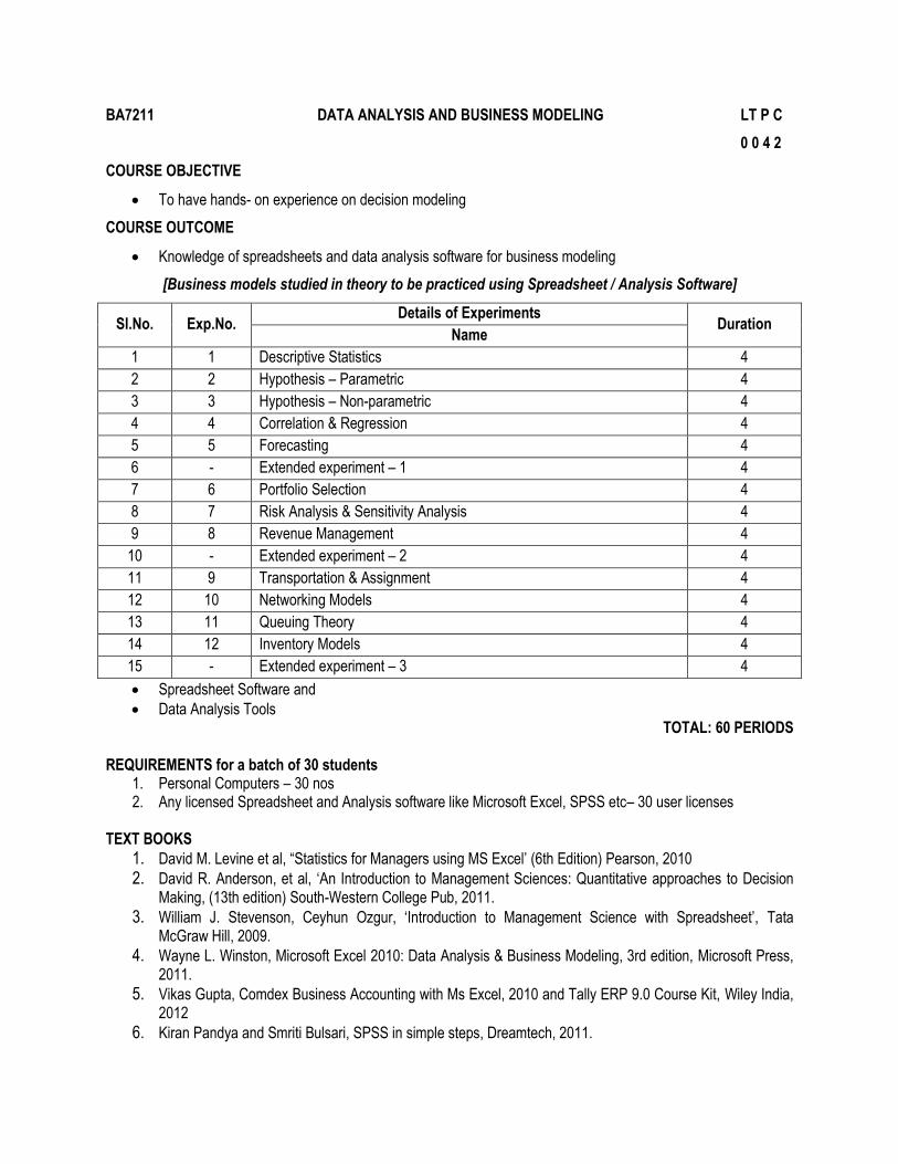
BA7211 DATA ANALYSIS AND BUSINESS MODELING LT P C

0 0 4 2

COURSE OBJECTIVE

To have hands- on experience on decision modeling

COURSE OUTCOME

Knowledge of spreadsheets and data analysis software for business modeling

[Business models studied in theory to be practiced using Spreadsheet / Analysis Software]

Sl.No. Exp.No. Details of Experiments

Duration Name

1 1 Descriptive Statistics 4

2 2 Hypothesis – Parametric 4

3 3 Hypothesis – Non-parametric 4

4 4 Correlation & Regression 4

5 5 Forecasting 4

6 - Extended experiment – 1 4

7 6 Portfolio Selection 4

8 7 Risk Analysis & Sensitivity Analysis 4

9 8 Revenue Management 4


11 9 Transportation & Assignment 4

12 10 Networking Models 4

13 11 Queuing Theory 4

14 12 Inventory Models 4


Spreadsheet Software and

Data Analysis Tools TOTAL: 60 PERIODS

REQUIREMENTS for a batch of 30 students

1. Personal Computers – 30 nos 2. Any licensed Spreadsheet and Analysis software like Microsoft Excel, SPSS etc– 30 user licenses

TEXT BOOKS

1. David M. Levine et al, “Statistics for Managers using MS Excel’ (6th Edition) Pearson, 2010

2. David R. Anderson, et al, ‘An Introduction to Management Sciences: Quantitative approaches to Decision Making, (13th edition) South-Western College Pub, 2011.

3. William J. Stevenson, Ceyhun Ozgur, ‘Introduction to Management Science with Spreadsheet’, Tata McGraw Hill, 2009.

4. Wayne L. Winston, Microsoft Excel 2010: Data Analysis & Business Modeling, 3rd edition, Microsoft Press, 2011.

5. Vikas Gupta, Comdex Business Accounting with Ms Excel, 2010 and Tally ERP 9.0 Course Kit, Wiley India, 2012

6. Kiran Pandya and Smriti Bulsari, SPSS in simple steps, Dreamtech, 2011.

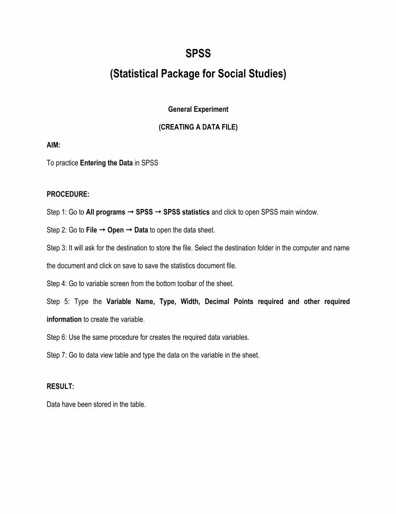
SPSS

(Statistical Package for Social Studies)

General Experiment

(CREATING A DATA FILE)

AIM:

To practice Entering the Data in SPSS

PROCEDURE:

Step 1: Go to All programs SPSS SPSS statistics and click to open SPSS main window.

Step 2: Go to File Open Data to open the data sheet.

Step 3: It will ask for the destination to store the file. Select the destination folder in the computer and name

the document and click on save to save the statistics document file.

Step 4: Go to variable screen from the bottom toolbar of the sheet.

Step 5: Type the Variable Name, Type, Width, Decimal Points required and other required

information to create the variable.

Step 6: Use the same procedure for creates the required data variables.

Step 7: Go to data view table and type the data on the variable in the sheet.

RESULT:

Data have been stored in the table.

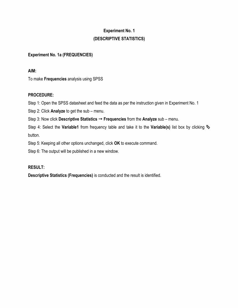
Experiment No. 1

(DESCRIPTIVE STATISTICS)

Experiment No. 1a (FREQUENCIES)

AIM:

To make Frequencies analysis using SPSS

PROCEDURE:

Step 1: Open the SPSS datasheet and feed the data as per the instruction given in Experiment No. 1

Step 2: Click Analyze to get the sub – menu.

Step 3: Now click Descriptive Statistics Frequencies from the Analyze sub – menu.

Step 4: Select the Variable1 from frequency table and take it to the Variable(s) list box by clicking

button.

Step 5: Keeping all other options unchanged, click OK to execute command.

Step 6: The output will be published in a new window.

RESULT:

Descriptive Statistics (Frequencies) is conducted and the result is identified.

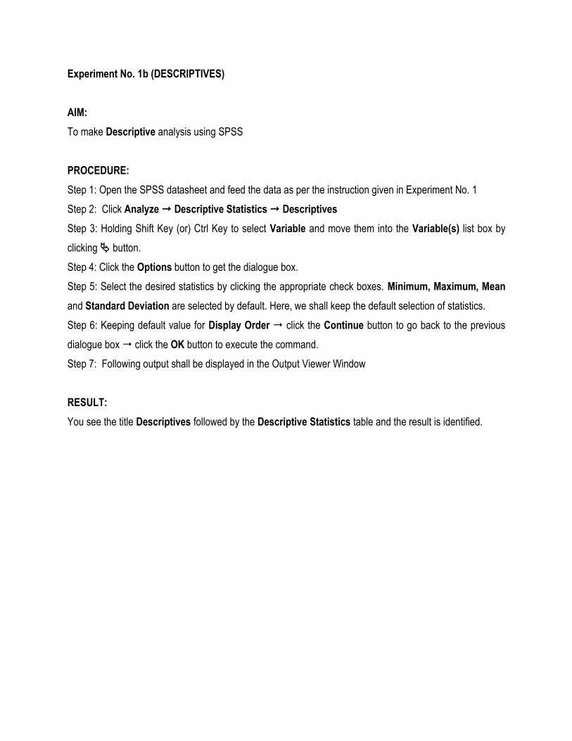
Experiment No. 1b (DESCRIPTIVES)

AIM:

To make Descriptive analysis using SPSS

PROCEDURE:


Step 2: Click Analyze Descriptive Statistics Descriptives

Step 3: Holding Shift Key (or) Ctrl Key to select Variable and move them into the Variable(s) list box by

clicking button.

Step 4: Click the Options button to get the dialogue box.

Step 5: Select the desired statistics by clicking the appropriate check boxes. Minimum, Maximum, Mean

and Standard Deviation are selected by default. Here, we shall keep the default selection of statistics.

Step 6: Keeping default value for Display Order click the Continue button to go back to the previous

dialogue box click the OK button to execute the command.

Step 7: Following output shall be displayed in the Output Viewer Window

RESULT:

You see the title Descriptives followed by the Descriptive Statistics table and the result is identified.

Experiment No. 1c (CROSSTABS) [an observation of Cross-tabulation]

AIM:

To make Crosstabs analysis using SPSS

PROCEDURE:


Step 2: Click Analyze Descriptive Statistics Crosstabs

Step 3: Select Variable1 and move it to the Rows list box and select Variable2 and move it to the

Columns list box.

Step 4: Click the Cells button to get the dialogue box.

Step 5: This allows you to add additional values to your table. Click the check box to select Observed,

Expected in the Counts frame; and the Row, Column and Total in the Percentage frame.

Step 6: Click the Continue button to go back to the previous dialogue box and then click the OK button

to execute the command.

Step 7: Following output shall be displayed in the Output Viewer Window

RESULT:

The output will display a heading Crosstabs followed by two tables – Case Processing Summary and

Variable1 * Variable2 Cross-tabulation and the result is identified.

Experiment No.2

(HYPOTHESIS – PARAMETRIC)

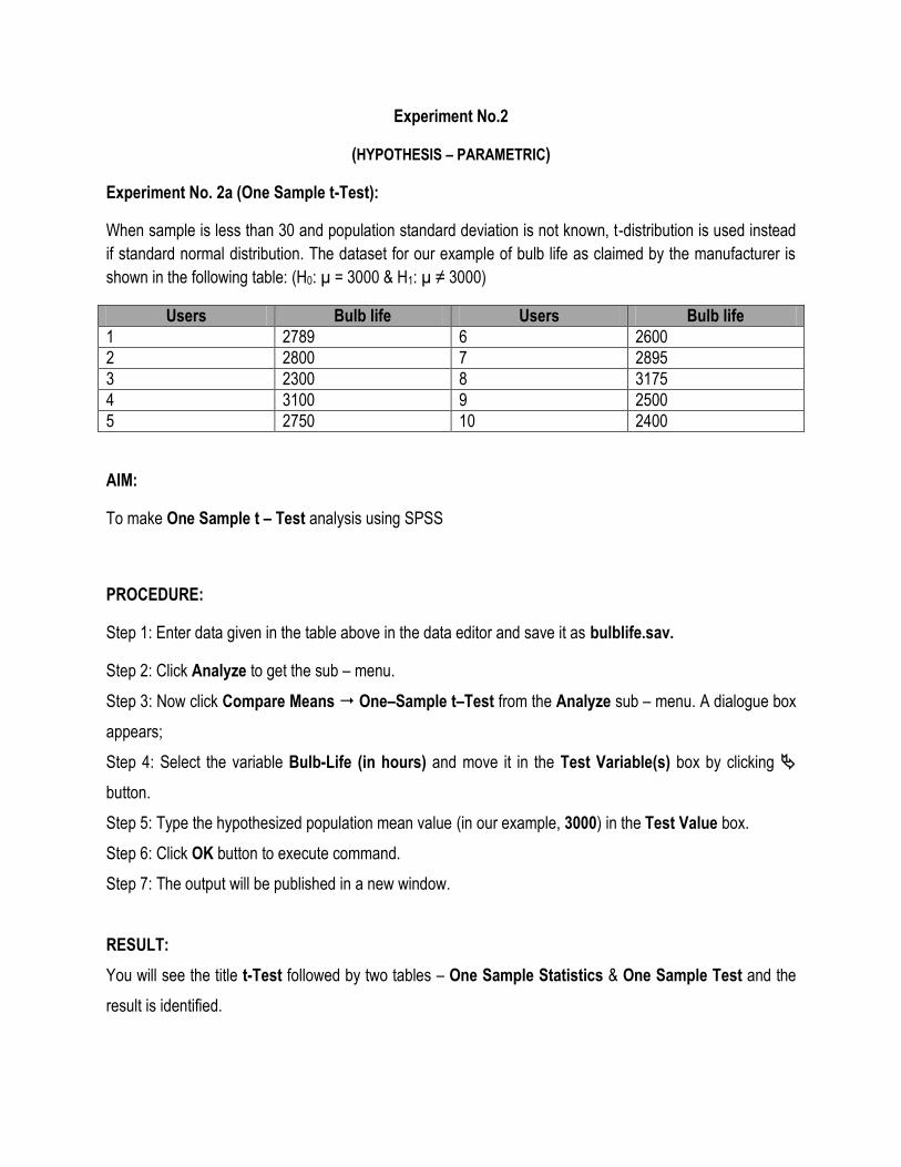
Experiment No. 2a (One Sample t-Test):

When sample is less than 30 and population standard deviation is not known, t-distribution is used instead

if standard normal distribution. The dataset for our example of bulb life as claimed by the manufacturer is

shown in the following table: (H0: µ = 3000 & H1: µ ≠ 3000)

Users Bulb life Users Bulb life

1 2789 6 2600

2 2800 7 2895

3 2300 8 3175

4 3100 9 2500

5 2750 10 2400

AIM:

To make One Sample t – Test analysis using SPSS

PROCEDURE:

Step 1: Enter data given in the table above in the data editor and save it as bulblife.sav.

Step 2: Click Analyze to get the sub – menu.

Step 3: Now click Compare Means One–Sample t–Test from the Analyze sub – menu. A dialogue box

appears;

Step 4: Select the variable Bulb-Life (in hours) and move it in the Test Variable(s) box by clicking

button.

Step 5: Type the hypothesized population mean value (in our example, 3000) in the Test Value box.

Step 6: Click OK button to execute command.

Step 7: The output will be published in a new window.

RESULT:

You will see the title t-Test followed by two tables – One Sample Statistics & One Sample Test and the

result is identified.

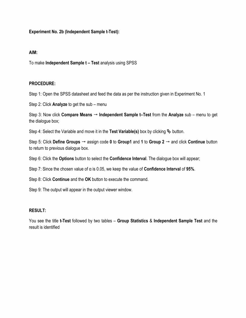
Experiment No. 2b (Independent Sample t-Test):

AIM:

To make Independent Sample t – Test analysis using SPSS

PROCEDURE:


Step 2: Click Analyze to get the sub – menu

Step 3: Now click Compare Means Independent Sample t–Test from the Analyze sub – menu to get

the dialogue box;

Step 4: Select the Variable and move it in the Test Variable(s) box by clicking button.

Step 5: Click Define Groups assign code 0 to Group1 and 1 to Group 2 and click Continue button

to return to previous dialogue box.

Step 6: Click the Options button to select the Confidence Interval. The dialogue box will appear;

Step 7: Since the chosen value of α is 0.05, we keep the value of Confidence Interval of 95%.

Step 8: Click Continue and the OK button to execute the command.

Step 9: The output will appear in the output viewer window.

RESULT:

You see the title t-Test followed by two tables – Group Statistics & Independent Sample Test and the

result is identified

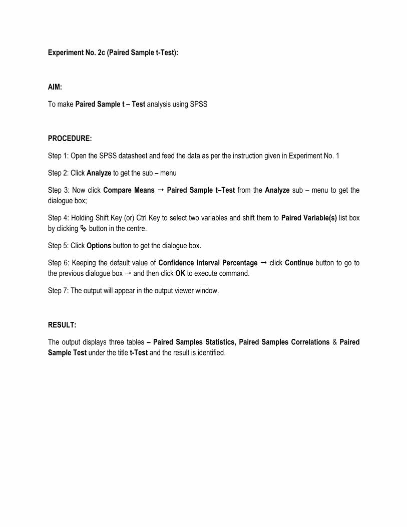
Experiment No. 2c (Paired Sample t-Test):

AIM:

To make Paired Sample t – Test analysis using SPSS

PROCEDURE:



Step 3: Now click Compare Means Paired Sample t–Test from the Analyze sub – menu to get the

dialogue box;

Step 4: Holding Shift Key (or) Ctrl Key to select two variables and shift them to Paired Variable(s) list box

by clicking button in the centre.

Step 5: Click Options button to get the dialogue box.

Step 6: Keeping the default value of Confidence Interval Percentage click Continue button to go to

the previous dialogue box and then click OK to execute command.

Step 7: The output will appear in the output viewer window.

RESULT:

The output displays three tables – Paired Samples Statistics, Paired Samples Correlations & Paired

Sample Test under the title t-Test and the result is identified.

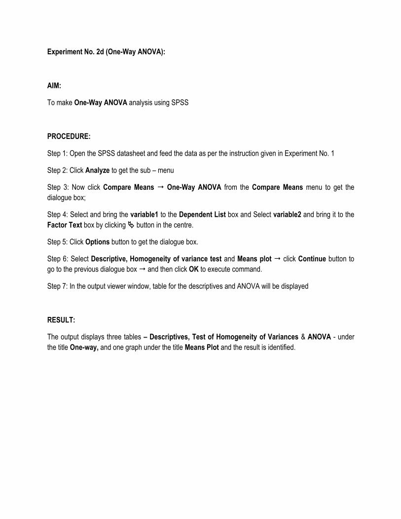
Experiment No. 2d (One-Way ANOVA):

AIM:

To make One-Way ANOVA analysis using SPSS

PROCEDURE:



Step 3: Now click Compare Means One-Way ANOVA from the Compare Means menu to get the

dialogue box;

Step 4: Select and bring the variable1 to the Dependent List box and Select variable2 and bring it to the

Factor Text box by clicking button in the centre.


Step 6: Select Descriptive, Homogeneity of variance test and Means plot click Continue button to

go to the previous dialogue box and then click OK to execute command.

Step 7: In the output viewer window, table for the descriptives and ANOVA will be displayed

RESULT:

The output displays three tables – Descriptives, Test of Homogeneity of Variances & ANOVA - under

the title One-way, and one graph under the title Means Plot and the result is identified.

Experiment No.3

(HYPOTHESIS – NON-PARAMETRIC)

Experiment No. 3a (Runs Test)

AIM:

To make Runs Test analysis using SPSS

PROCEDURE:



Step 3: Now click Non-parametric Legacy Dialogues Runs to get the dialogue box;

Step 4: Select Variable and move it to Test Variable List box by clicking button.


Step 6: Select the desired statistics by clicking the appropriate check boxes Descriptive and Quartiles

Check boxes. Here, we shall keep the default selection of statistics.

Step 7: Click Continue button to go to the previous dialogue box and then click OK to execute

command.

Step 7: The output will be displayed in the output viewer window.

RESULT:

The output displays two tables – Descriptive Statistics and Runs Test are displayed under the heading

NPar Tests and the result is identified.

Experiment No. 3b (Chi – Square Test)

AIM:

To make Chi – Square Test analysis using SPSS

PROCEDURE:



Step 3: Click Descriptive Statistics Crosstabs to get the dialogue box.

Step 4: Select Variable1 and move it to the Rows list box and select Variable2 and move it to the Columns

list box.

Step 5: Click Statistics button to get the dialogue box.

Step 6: This allows you to add additional values to your table. Click the check box to select Chi-Square

click Continue to return to the previous dialogue box.

Step 7: Keeping all other options unchanged, click OK button to execute the command.

Step 8: The output will be appear in output viewer window.

RESULT:

Three tables – Case Processing Summary and Variable1 * Variable2 Cross-tabulation and Chi-Square

Tests – are generated under the heading Crosstabs on executing the command for Chi-square test and

the result is identified.

Experiment No. 3c (Mann-Whitney U Test)

AIM:

To make Mann-Whitney U Test analysis using SPSS

PROCEDURE:



Step 3: Click Nonparametric Legacy 2 Independent Samples to get the dialogue box.

Step 4: Select Variable and move it to Test Variable List box by clicking button.

Step 5: Click Define Groups assign code 0 to Group1 and 1 to Group 2 and click Continue button

to return to previous dialogue box.


Step 7: Select Descriptive and Quartiles options in Statistics frame by clicking them.

Step 8: Click Continue button to go back to the previous dialogue box and keeping all other options

unchanged.

Step 9: Click OK to execute the command.


RESULT:

Under the title – Npar Test, a table – Descriptive Statistics are displayed. Just below this table, two more

tables – Ranks and Test Statistics are displayed under the heading Mann-Whitney Test and the result is

identified.

Experiment No. 3d (Wilcoxon Signed Rank Test)

AIM:

To make Wilcoxon Signed Rank Test analysis using SPSS

PROCEDURE:



Step 3: Click Nonparametric Legacy 2 Related Samples to get the dialogue box.

Step 4: Holding Shift Key (or) Ctrl Key to select two variables and shift them to Test Pairs list box by

clicking button in the centre.


Step 7: Select Descriptive and Quartiles by clicking on respective check boxes.


unchanged.



RESULT:

Descriptive Statistics table is displayed under the heading Npar Tests and two more tables – Ranks and

Test Statistics are displayed under the heading Wilcoxon Signed Ranks Test and the result is identified.

Experiment No. 3e (Kruskal - Wallis Test)

AIM:

To make Kruskal - Wallis Test analysis using SPSS

PROCEDURE:



Step 3: Click Nonparametric Legacy K Independent Samples to get the dialogue box.

Step 4: Select the Variable1 and move it in the Test Variable(s) and Variable2 in the Grouping Variable

box by clicking button.

Step 5: Click Define Range type in 1 in Minimum and 3 in Maximum and click Continue button to

return to previous dialogue box.


Step 7: Select Descriptive and Quartiles by clicking on respective check boxes.


unchanged.



RESULT:

Descriptive Statistics table is displayed under the heading Npar Tests and two more tables – Ranks and

Test Statistics are displayed under the heading Kruskal-Wallis Test and the result is identified.

Experiment No. 4

(CORRELATION & REGRESSION)

Experiment No. 4a (Correlations)

AIM:

To make correlation analysis using SPSS

PROCEDURE:

Step 1: Open the SPSS datasheet and feed the data as per the instruction given in Experiment No.1


Step 3: Click Correlate Bivariate to get the dialogue box.

Step 4: Holding Shift Key (or) Ctrl Key to select two or more variables and move these variables to the

Variables box by clicking button in the centre.


Step 6: To find out Means and standard deviations for each of the selected variables, select appropriate

check boxes in the Statistics frame.


unchanged.



RESULT:

Under the major heading – Correlations, a table titled Correlations is displayed and the result where

identified.

Experiment No. 4b (Regression)

AIM:

To make Multiple Regression analysis using SPSS

PROCEDURE:

Step 1: Open the SPSS datasheet and feed the data as per the instruction given in Experiment No.1


Step 3: Click Regression Linear to get the dialogue box.

Step 4: Select Variable1 and move it to Dependent text box and holding Shift Key (or) Ctrl Key to select

two or more Variables and bring these variables to the Independent(s) list box by clicking button in the

centre.

Step 5: Keeping other options unchanged click OK button to execute command.


RESULT:

Under the title Regression, four tables – Variables Entered and Removed, Model Summary, ANOVA

and Coefficients – will be displayed and the result where identified.

Experiment No. 5

(FORECASTING)

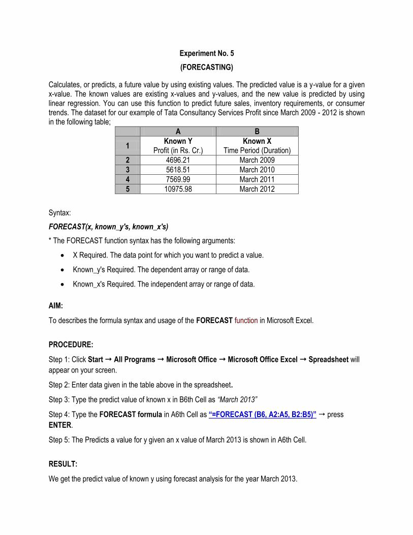
Calculates, or predicts, a future value by using existing values. The predicted value is a y-value for a given x-value. The known values are existing x-values and y-values, and the new value is predicted by using linear regression. You can use this function to predict future sales, inventory requirements, or consumer trends. The dataset for our example of Tata Consultancy Services Profit since March 2009 - 2012 is shown in the following table;

A B

1 Known Y

Profit (in Rs. Cr.) Known X

Time Period (Duration)

2 4696.21 March 2009

3 5618.51 March 2010

4 7569.99 March 2011

5 10975.98 March 2012

Syntax:

FORECAST(x, known_y's, known_x's)

* The FORECAST function syntax has the following arguments:

X Required. The data point for which you want to predict a value.

Known_y's Required. The dependent array or range of data.

Known_x's Required. The independent array or range of data.

AIM:

To describes the formula syntax and usage of the FORECAST function in Microsoft Excel.

PROCEDURE:

Step 1: Click Start All Programs Microsoft Office Microsoft Office Excel Spreadsheet will

appear on your screen.

Step 2: Enter data given in the table above in the spreadsheet.

Step 3: Type the predict value of known x in B6th Cell as “March 2013”

Step 4: Type the FORECAST formula in A6th Cell as “=FORECAST (B6, A2:A5, B2:B5)” press

ENTER.

Step 5: The Predicts a value for y given an x value of March 2013 is shown in A6th Cell.

RESULT:

We get the predict value of known y using forecast analysis for the year March 2013.

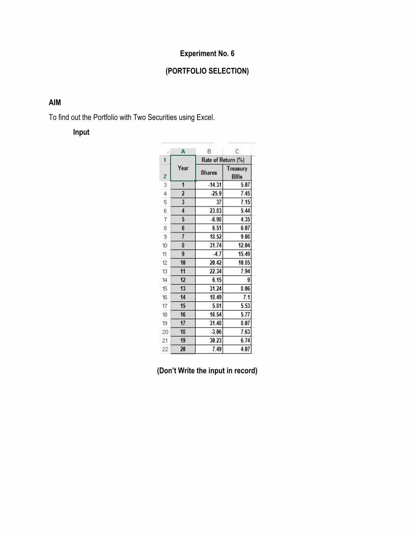
Experiment No. 6

(PORTFOLIO SELECTION)

AIM

To find out the Portfolio with Two Securities using Excel.

Input

(Don’t Write the input in record)

PROCEDURE

Step 1: To open Ms-Excel window click Ms-Excel from programme.

Step 2: Click new document from the office button to create a new spread sheet

Step 3: Type the problem in rows and columns

Step 4: For Portfolio Construction with Two Securities computations, you need three main values Mean,

Standard Deviation, Correlation.

Step 5: To Calculate Mean of Securities for 20 years type the Formula in the Formula bar as

=SUM(B3:B22)/20 for both Securities

Step 6: To Calculate Standard Deviation for 20 years type the Formula in the Formula bar as

=STDEV(B3:B22) for both Securities.

Step 7: To Calculate Correlation for 20 years type the Formula in the Formula bar as

=CORREL(B3:B22,C3:C22).

Step 8: To identify Optimal Portfolio Create a different combination of investment as W1 and W2 in Excel.

Step 9: To identify Optimal Portfolio Create a different combination of investment calculate Standard

Deviation and mean for each Combination

Step 10: To Calculate Standard Deviation for 2 securities type the Formula in the Formula bar as

=SQRT(E5^2*$B$24^2+F5^2*$C$24^2+2*$B$26*E5*F5*$B$24*$C$24).

Step 11: To Calculate mean for 2 securities type the Formula in the Formula bar as

=E5*$B$23+F5*$C$23.

RESULT:

Thus the Selection of Portfolio with Two Securities has been solved in Excel.

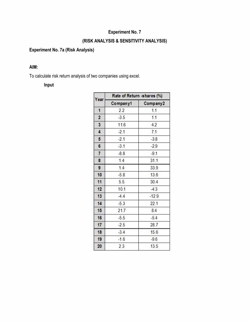
Experiment No. 7

(RISK ANALYSIS & SENSITIVITY ANALYSIS)

Experiment No. 7a (Risk Analysis)

AIM:

To calculate risk return analysis of two companies using excel.

Input

PROCEDURE:

Step 1: Click Start Programs MS Office MS Excel

Step 2: Enter the data (Given in Input) in the excel sheet.

Step 3: Insert the “Data Analysis” option to click File Add-Ins Select Analysis ToolPak and then

Excel Add-ins in Manage Click Go Add-Ins box will appear Select Analysis ToolPak

then click OK. (Note: can't find the Data Analysis button? Click here to load the Analysis ToolPak add-in.)

Step 4: Goto Data Analysis Descriptive Statistics Descriptive Statistics OK.

Step 5: A pop up menu appears. In that select the “Input range”, to drag the problem except year.

Step 6: Select the “Lables in first row” & “Summary Statistics”. Then move to output options, Click

“Output range”, select the empty cells OK.

Step 7: Then Risk Analysis for the company will displayed in the output screen.

RESULT:

We can see standard deviation, sample variance and Range are all greater for company 2 when compared

to company 1. Hence company 1 is better for investment than company 2.

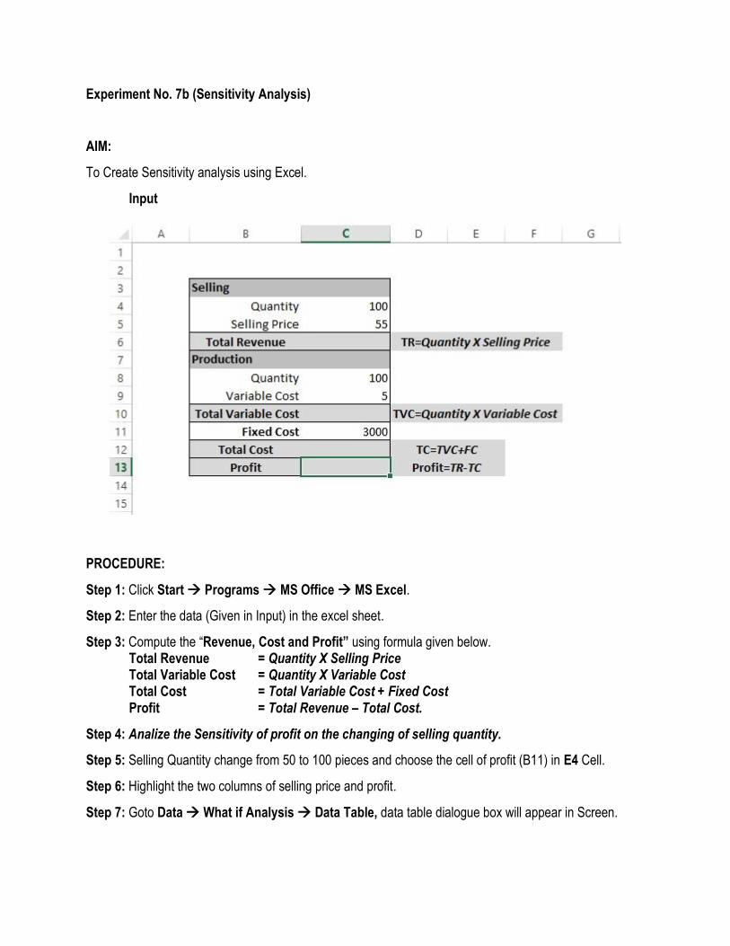
http://www.excel-easy.com/data-analysis/analysis-toolpak.html

Experiment No. 7b (Sensitivity Analysis)

AIM:

To Create Sensitivity analysis using Excel.

Input

PROCEDURE:

Step 1: Click Start Programs MS Office MS Excel.

Step 2: Enter the data (Given in Input) in the excel sheet.

Step 3: Compute the “Revenue, Cost and Profit” using formula given below. Total Revenue = Quantity X Selling Price Total Variable Cost = Quantity X Variable Cost Total Cost = Total Variable Cost + Fixed Cost Profit = Total Revenue – Total Cost.

Step 4: Analize the Sensitivity of profit on the changing of selling quantity.

Step 5: Selling Quantity change from 50 to 100 pieces and choose the cell of profit (B11) in E4 Cell.

Step 6: Highlight the two columns of selling price and profit.

Step 7: Goto Data What if Analysis Data Table, data table dialogue box will appear in Screen.

Step 8: Choose the Selling Quantity in “Column Input Cell”, because the selling price is on the column

then click OK.

Step 9: Analyize the Sensitivity of Profit on the changing percentage of decrease or increase of

fixed cost.

Step 10: Fixed cost will change from –15 % (decrease) to +10% (increase) and enter the fixed cost

amount 3000 in “D15” cell.

Step 11: In “E16” cell, enter the formula =$D$15*(1+D16) to calculate the fixed cost when in decrease or

increase and choose the cell of profit (B11) in “F15” Cell.

Step 12: Highlight the column fixed cost & profit and follow the step no. 7

Step 13: Choose the fixed cost in “Column Input Cell”, because the fixed cost is on the column then

click OK.

Step 14: Analize the Sensitivity of profit on the changing of selling quantity and variable cost.

Step 15: Selling price change from 50 to 100 pieces and variable cost changes from 3 to 7.

Step 16: “E25” Cell is the cell of profit that need to be analized. It must be the intersection of selling

quantity and then highlight the range and follow the step no. 7.

Step 17: Choose Row Input Cell is “Variable Cost” and Column Input Cell is “Selling Quantity”

then click OK.

RESULT:

Thus the calculated Sensitivity analysis using excel successfully.

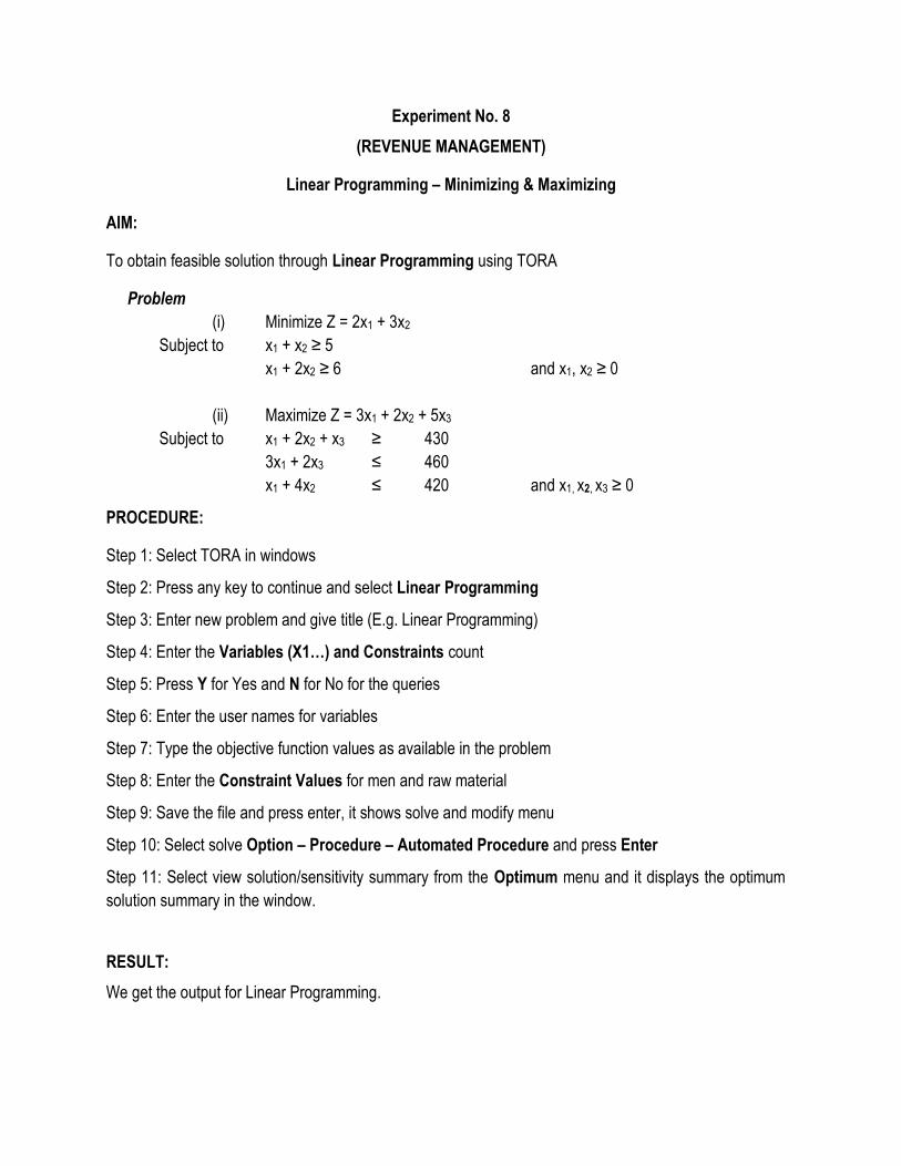
Experiment No. 8

(REVENUE MANAGEMENT)

Linear Programming – Minimizing & Maximizing

AIM:

To obtain feasible solution through Linear Programming using TORA

Problem

(i) Minimize Z = 2x1 + 3x2

Subject to x1 + x2 ≥ 5

x1 + 2x2 ≥ 6 and x1, x2 ≥ 0

(ii) Maximize Z = 3x1 + 2x2 + 5x3

Subject to x1 + 2x2 + x3 ≥ 430

3x1 + 2x3 ≤ 460

x1 + 4x2 ≤ 420 and x1, x2, x3 ≥ 0

PROCEDURE:

Step 1: Select TORA in windows

Step 2: Press any key to continue and select Linear Programming

Step 3: Enter new problem and give title (E.g. Linear Programming)

Step 4: Enter the Variables (X1…) and Constraints count

Step 5: Press Y for Yes and N for No for the queries

Step 6: Enter the user names for variables

Step 7: Type the objective function values as available in the problem

Step 8: Enter the Constraint Values for men and raw material

Step 9: Save the file and press enter, it shows solve and modify menu

Step 10: Select solve Option – Procedure – Automated Procedure and press Enter

Step 11: Select view solution/sensitivity summary from the Optimum menu and it displays the optimum

solution summary in the window.

RESULT:

We get the output for Linear Programming.

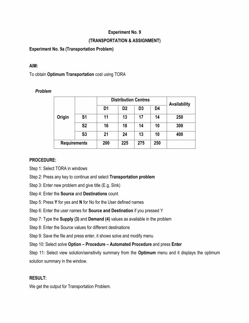
Experiment No. 9

(TRANSPORTATION & ASSIGNMENT)

Experiment No. 9a (Transportation Problem)

AIM:

To obtain Optimum Transportation cost using TORA

Problem

Origin

Distribution Centres Availability

D1 D2 D3 D4

S1 11 13 17 14 250

S2 16 18 14 10 300

S3 21 24 13 10 400

Requirements 200 225 275 250

PROCEDURE:


Step 2: Press any key to continue and select Transportation problem

Step 3: Enter new problem and give title (E.g. Sink)

Step 4: Enter the Source and Destinations count

Step 5: Press Y for yes and N for No for the User defined names

Step 6: Enter the user names for Source and Destination if you pressed Y

Step 7: Type the Supply (3) and Demand (4) values as available in the problem

Step 8: Enter the Source values for different destinations





RESULT:

We get the output for Transportation Problem.

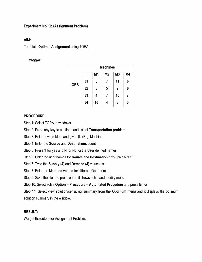
Experiment No. 9b (Assignment Problem)

AIM:

To obtain Optimal Assignment using TORA

Problem

JOBS

Machines

M1 M2 M3 M4

J1 5 7 11 6

J2 8 5 9 6

J3 4 7 10 7

J4 10 4 8 3

PROCEDURE:


Step 2: Press any key to continue and select Transportation problem

Step 3: Enter new problem and give title (E.g. Machine)

Step 4: Enter the Source and Destinations count

Step 5: Press Y for yes and N for No for the User defined names

Step 6: Enter the user names for Source and Destination if you pressed Y

Step 7: Type the Supply (4) and Demand (4) values as 1

Step 8: Enter the Machine values for different Operators





RESULT:

We get the output for Assignment Problem.

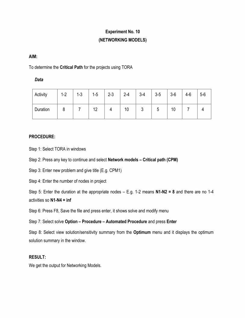
Experiment No. 10

(NETWORKING MODELS)

AIM:

To determine the Critical Path for the projects using TORA

Data

Activity 1-2 1-3 1-5 2-3 2-4 3-4 3-5 3-6 4-6 5-6

Duration 8 7 12 4 10 3 5 10 7 4

PROCEDURE:


Step 2: Press any key to continue and select Network models – Critical path (CPM)

Step 3: Enter new problem and give title (E.g. CPM1)

Step 4: Enter the number of nodes in project

Step 5: Enter the duration at the appropriate nodes – E.g. 1-2 means N1-N2 = 8 and there are no 1-4

activities so N1-N4 = inf

Step 6: Press F8, Save the file and press enter, it shows solve and modify menu




RESULT:

We get the output for Networking Models.

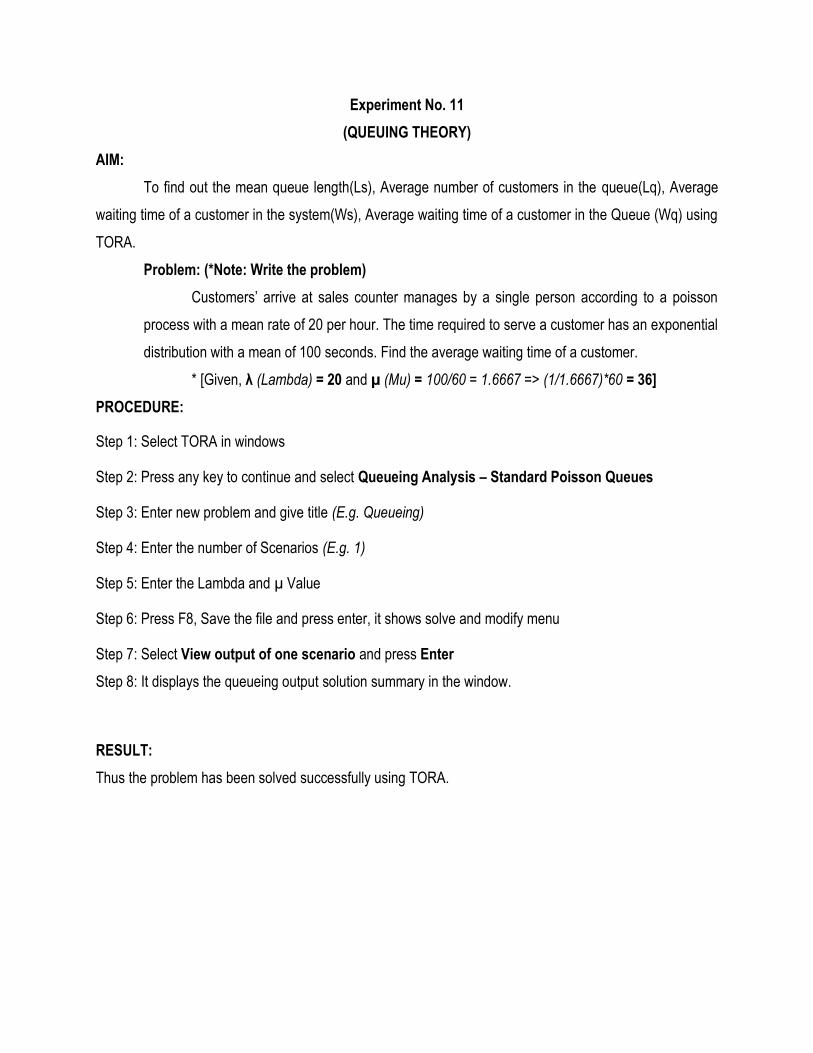
Experiment No. 11

(QUEUING THEORY)

AIM:

To find out the mean queue length(Ls), Average number of customers in the queue(Lq), Average

waiting time of a customer in the system(Ws), Average waiting time of a customer in the Queue (Wq) using

TORA.

Problem: (*Note: Write the problem)

Customers’ arrive at sales counter manages by a single person according to a poisson

process with a mean rate of 20 per hour. The time required to serve a customer has an exponential

distribution with a mean of 100 seconds. Find the average waiting time of a customer.

* [Given, λ (Lambda) = 20 and µ (Mu) = 100/60 = 1.6667 => (1/1.6667)*60 = 36]

PROCEDURE:


Step 2: Press any key to continue and select Queueing Analysis – Standard Poisson Queues

Step 3: Enter new problem and give title (E.g. Queueing)

Step 4: Enter the number of Scenarios (E.g. 1)

Step 5: Enter the Lambda and µ Value

Step 6: Press F8, Save the file and press enter, it shows solve and modify menu

Step 7: Select View output of one scenario and press Enter

Step 8: It displays the queueing output solution summary in the window.

RESULT:

Thus the problem has been solved successfully using TORA.

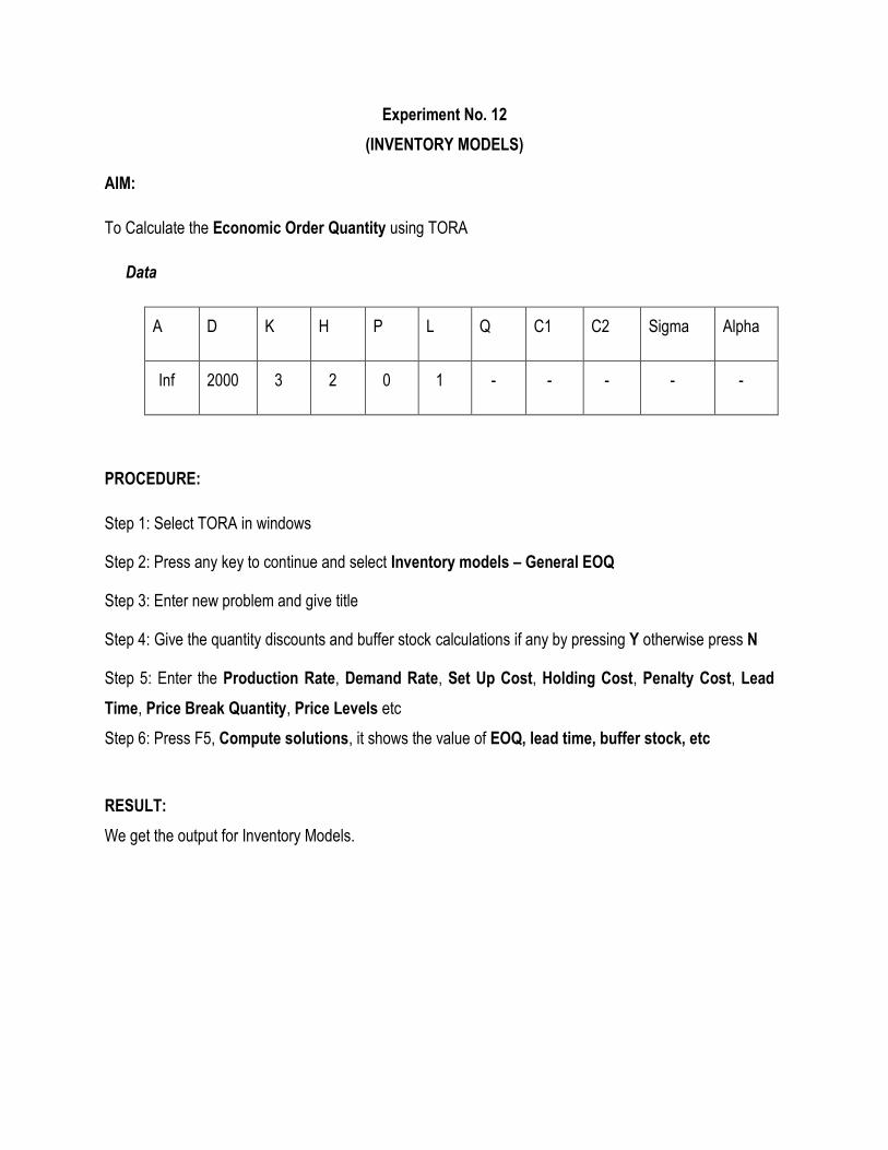
Experiment No. 12

(INVENTORY MODELS)

AIM:

To Calculate the Economic Order Quantity using TORA

Data

A D K H P L Q C1 C2 Sigma Alpha

Inf 2000 3 2 0 1 - - - - -

PROCEDURE:


Step 2: Press any key to continue and select Inventory models – General EOQ

Step 3: Enter new problem and give title

Step 4: Give the quantity discounts and buffer stock calculations if any by pressing Y otherwise press N

Step 5: Enter the Production Rate, Demand Rate, Set Up Cost, Holding Cost, Penalty Cost, Lead

Time, Price Break Quantity, Price Levels etc

Step 6: Press F5, Compute solutions, it shows the value of EOQ, lead time, buffer stock, etc

RESULT:

We get the output for Inventory Models.

E.G.S. PILLAY ENGINEERING COLLEGE, NAGAPATTINAM 611...

Documents

Transcript of E.G.S. PILLAY ENGINEERING COLLEGE, NAGAPATTINAM 611...