EGR 106 – Week 4 – Math on Arrays

Linear algebraic operations:– Multiplication– Division

Row/column based operations

Rest of chapter 3

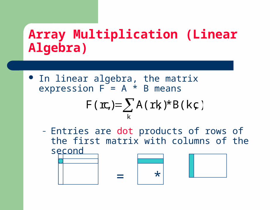
Array Multiplication (Linear Algebra)

In linear algebra, the matrix expression F = A * B means

– Entries are dot products of rows of the first matrix with columns of the second

= *

k

c)B(k,*k)A(r,c)F(r,

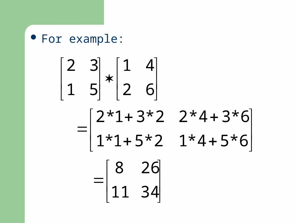
For example:

3411

268

6*54*12*51*1

6*34*22*31*2

62

41

51

32

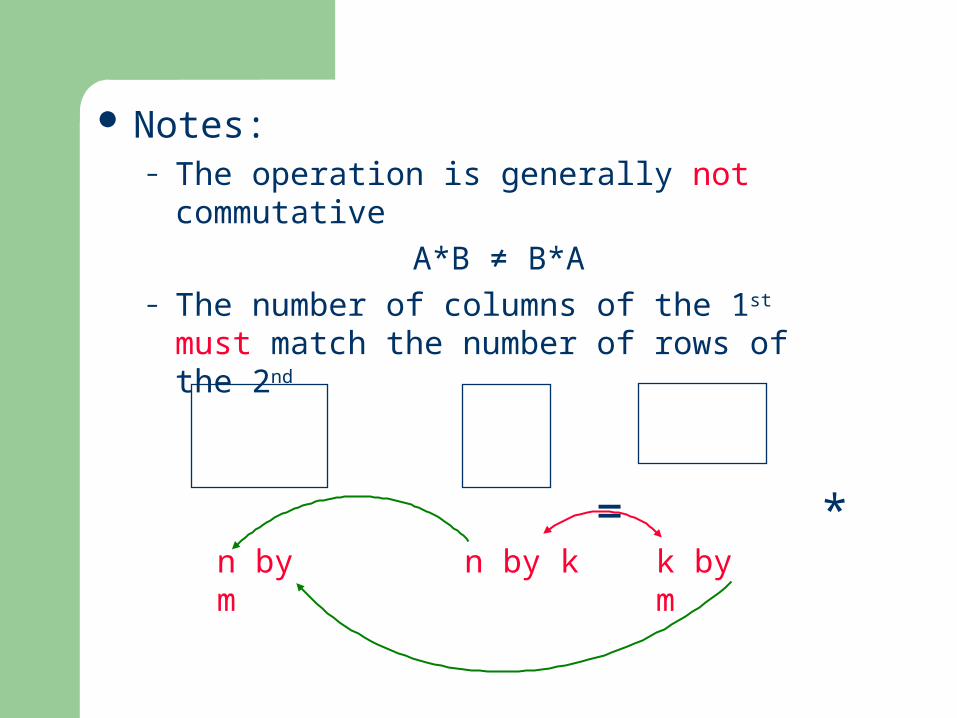
Notes: – The operation is generally not commutative

A*B ≠ B*A– The number of columns of the 1st must match

the number of rows of the 2nd

= *

n by k k by mn by m

For example, here multiplication works both ways, but is not commutative:

quite different!

And here it doesn’t work at all:

Application of Multiplication

Application of matrix multiplication: n simultaneous equations in m unknowns (the x’s)

nmnmnn

m

mm

bxaxaxa

bxaxaxa

bxaxaxa

1211

211222121

11212111

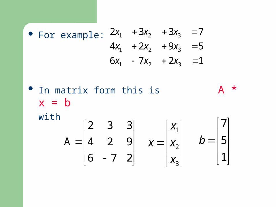
For example:

In matrix form this is A * x = bwith

3

2

1

x

x

x

x

276

924

332

A

1

5

7

2

9

3

7

2

3

6

4

2

3

3

3

2

2

2

1

1

1

x

x

x

x

x

x

x

x

x

1

5

7

b

In general: A * x = b

– A is n by m– x is m by 1– b is n by 1

nmnmnn

m

mm

bxaxaxa

bxaxaxa

bxaxaxa

1211

211222121

11212111

column vectors (lower case)

Usages – finding: – cable tensions in statics– fluid flow in piping – heat flow in thermodynamics

– e.g.

v

– currents in circuits– traffic flow– economics

i1 i2

R1

R2

R3

0

*2

1

322

221 v

i

i

RRR

RRR

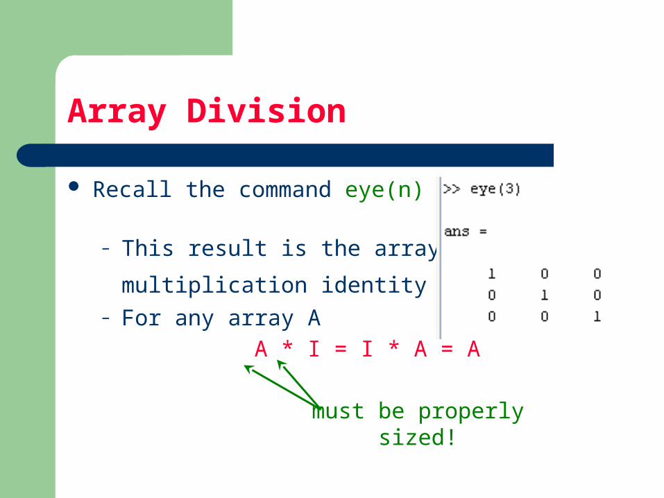
Array Division

Recall the command eye(n)

– This result is the array

multiplication identity matrix I– For any array A

A * I = I * A = A

must be properly sized!

Imagine that for square arrays A and B we have

A * B = B * A = I

then we call them inverses

A = B–1 B = A–1

In Matlab: A ^ -1 or inv(A)

When does A–1 exist?– A is square– A has a non-zero determinant (det(A))

For example:

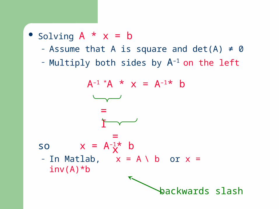
Solving A * x = b – Assume that A is square and det(A) ≠ 0

– Multiply both sides by A–1 on the left

A–1 *A * x = A–1* b

so x = A–1* b– In Matlab, x = A \ b or x = inv(A)*b

= I

= x

backwards slash

For example:

Check your work:

General Linear Equation Solving (not in the book!)

Problem types:– overdetermined– underdetermined

Solution methods:– Cramer's method – Gaussian elimination– inverse matrix– others

Solution situations:– non-singular:

one unique solution – singular:

no solutionmany solutions

MatLab does them all

Vector Based Operations

Some operations analyze a vector to yield a single value. For example:

sums the elements

Other operations for a vector A:

– Minimum: min(A)– Maximum: max(A)– Median: median(A)– Mean or average: mean(A)– Standard deviation: std(A)– Product of the elements: prod(A)

Some operators yield two results:

– min and max can

yield both the value and its location

– default is the first result

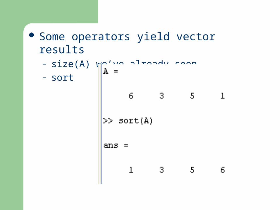
Some operators yield vector results – size(A) we’ve already seen – sort

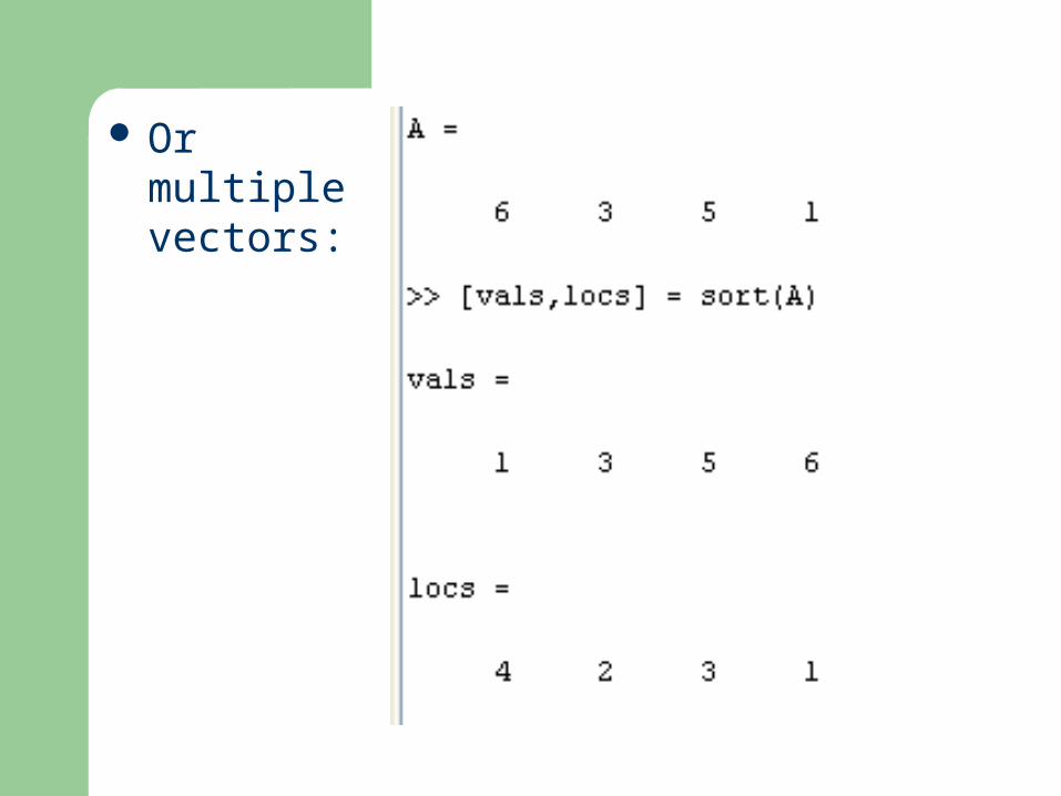
Or multiple vectors:

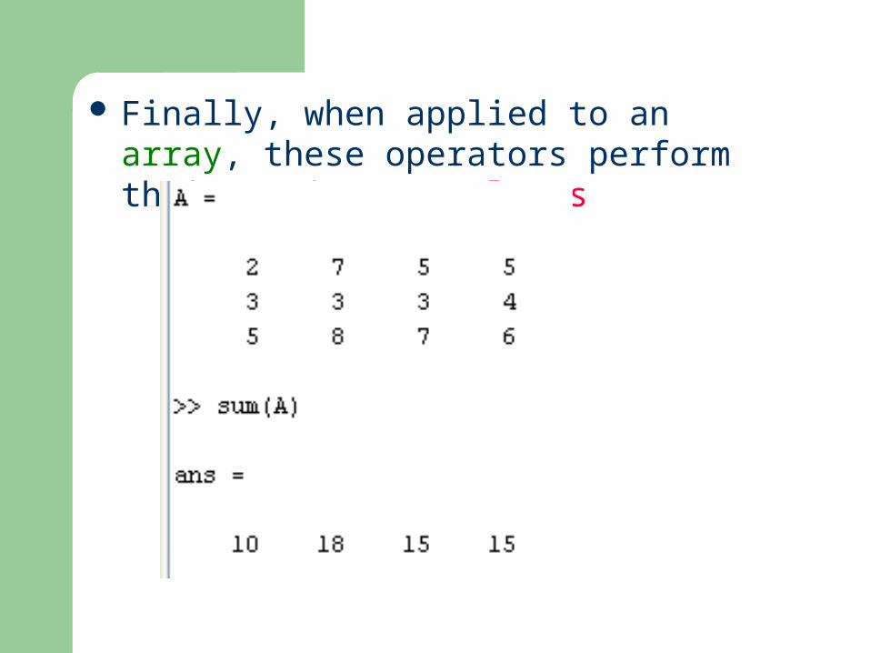
Finally, when applied to an array, these operators perform their action on columns

Unless you instruct it to work on rows!

the 2 means “use the 2nd dimension” i.e.

spanning the columns

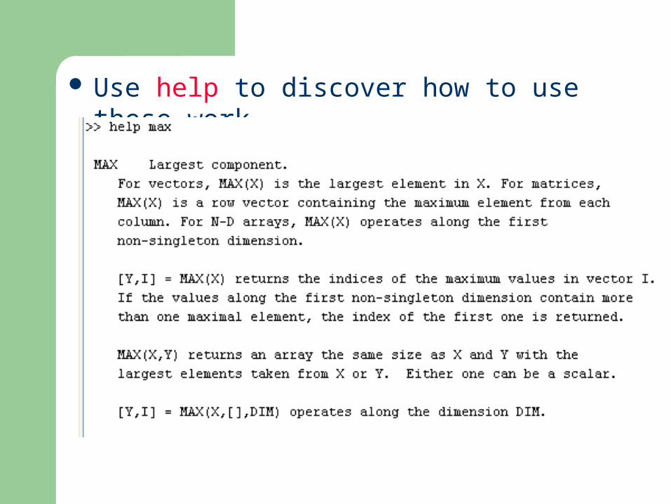
Use help to discover how to use these work