Efficient Algorithms for Route Planning Problems on Road...
103
Efficient Algorithms for Route Planning Problems on Road Networks P H.D. THESIS IN COMPUTER S CIENCE DOKTORARBEIT IN I NFORMATIK TESI DI DOTTORATO DI RICERCA IN I NFORMATICA Theodoros Chondrogiannis
Transcript of Efficient Algorithms for Route Planning Problems on Road...
Efficient Algorithms for Route Planning
Problems on Road Networks
PH.D. THESIS IN COMPUTER SCIENCE
DOKTORARBEIT IN INFORMATIK
TESI DI DOTTORATO DI RICERCA IN INFORMATICA
Theodoros Chondrogiannis


Relatore - Doktorvater - Faculty Advisor: Prof. Dr. Johann Gamper
Examination committee:Prof. Kyriakos Mouratidis (chair), Singapore Management UniversityProf. Dr. Matthias Renz, George Mason UniversityProf. Johann Gamper (secretary), Free University of Bozen-BolzanoProf. Dr. Gunther Specht (chair substitute member), University of InnsbruckProf. Dr. Peer Kroger (substitute member), Ludwig Maximillians University of MunchenProf. Prof. Alessandro Artale (internal substitute member), Free University of Bozen-Bolzano
Keywords: Shortest Path, Graph Partitioning, Spatial Network Queries, WebGIS, MultimodalNetworks, Alternative Routing
ACM categories: DATA STRUCTURES, Algorithms, Spatial databases and GIS
Copyright c� 2017 by Theodoros Chondrogiannis
This work is licensed under the Creative Commons Attribution-Noncommercial-Share Alike3.0 License. To view a copy of this license, visit http://creativecommons.org/licenses/by-nc-sa/3.0/ or send a letter to Creative Commons, 543 Howard Street, 5th floor, San Francisco,California, 94105, USA.


Acknowledgments
First and foremost, I want to thank my supervisor Prof. Johann Gamper for all his contri-butions of time, ideas and funding to make my PhD experience exciting and productive. Hehas taught me how deepened research in the field of computer science is done. The joy andenthusiasm he has for his research was truly inspiring for me.
Second, I would also like to thank Dr. Panagiotis Bouros and Prof. Dr. Ulf Leser for theircontributions to my work. I am grateful to them for inviting me to Humboldt-Universitat zuBerlin during my study period abroad. They taught me how important it is to collaborate andexchange ideas with other researchers in order to conduct top level research. My collaborationwith them was an invaluable experience.
Third, I would like to thank all of my group members and colleagues (current and for-mer ones), for their valuable inputs during the inspirational discussions in our seminars or inthe coffee breaks. Many thanks also to my colleagues from the University of Zurich and theUniversity of Salzburg for the valuable inputs during our annual retreat seminars.
I would also like to thank Roberto Cavaliere and Patrick Ohnewein from IDM Sudtirol fortheir collaboration and their feedback during the development of the prototype system MoTrISpresented in this thesis.
Also many thanks to Maria for her constant support and for putting up with me during thelast year of my PhD studies, especially during the time I was writing my thesis.
Lastly, I would like to thank my family for all their love and encouragement. Especially myparents Petros and Eleftheria, and my grandfather Nikos, who raised me with a love of scienceand taught me how to pursue with passion any targets I set in my life. Thank you.
Bolzano, 15/5/2017Theodoros Chondrogiannis
v

Abstract
Route planning services have become very popular over the past decade. The increasedavailability of road network data has triggered the development of a variety of new applications.In this spirit, the overall goal of this thesis is to propose efficient algorithms for tackling routeplanning problems on road networks. In particular, we study the following two problems:(a) the efficient processing of distance and shortest path queries and (b) the computation ofdissimilar yet short alternative paths.
Distance and shortest path queries can be used as building blocks for more complex querieson road networks. Therefore, the efficient processing of both types of queries is of great im-portance. However, most state-of-the-art methods focus solely on one type of query and donot efficiently support the other. To address this shortcoming, we propose the Partition-basedframework for Distance and Shortest Path queries (ParDiSP), which combines ideas from state-of-the-art approaches in a novel way and provides exceptional query times for both distanceand shortest path queries. Our framework first partitions the road network into components.Then exploits the properties of the partitioning for precomputations to boost query process-ing. ParDiSP answers distance queries solely by accessing precomputed distance tables andsignificantly limits the part of the road network that has to be accessed to process shortest pathqueries. A detailed experimental evaluation shows that: ParDiSP outperforms the state-of-the-art for shortest path queries, is comparable to the state-of-the-art for distance queries, and,for mixed query loads containing both distance and shortest path queries, outperforms even acombination of the best methods for each query type.
In many real-world scenarios though, returning only the shortest path is not enough. Mostcommercial navigation systems recommend, apart from the shortest path, a number of alterna-tive paths with different characteristics, leaving the final decision to the user. In this context,we formally introduce the k-Shortest Paths with Limited Overlap (k-SPwLO) problem seekingto compute k alternative paths which are as short as possible and sufficiently dissimilar basedon a user-controlled similarity threshold. We present three algorithms that examine the pathsfrom a source s to a target t in increasing order of their length and progressively construct theresult set. First, the baseline algorithm BSL builds upon the computation of K-shortest paths.Second, OnePass traverses the network to expand every path from the source that qualifiesthe similarity constraint. Third, MultiPass traverses the network k�1 times and employs two
vii
pruning criteria to reduce the number of paths that have to be examined. In an extensive ex-perimental evaluation we show that MultiPass is the fastest algorithm for processing k-SPwLOqueries as it outperforms both BSL and OnePass and, in most cases, by a large margin.
To achieve scalability, we also propose two heuristic algorithms that trade accuracy forefficiency. OnePass+ employs the same pruning criteria as MultiPass, but traverses the networkonly once. Therefore, some paths might be lost that otherwise would be part of the solution.ESX computes alternative paths by incrementally removing edges from the road network andrunning shortest path queries on the updated network. An extensive experimental analysison real road networks shows that OnePass+ runs significantly faster than MultiPass with itsresult being close to the exact solution, and ESX is faster than OnePass+ (though slightly lessaccurate) and scales for large road networks and large values of k.
Finally, we present MoTrIS, a service-oriented Multimodal Transport Information Systemfor routing services on road and transportation networks. We have implemented and integratedtwo of the algorithms presented in this thesis into MoTrIS: ParDiSP for processing distanceand shortest path queries, and ESX to recommend alternative paths. In addition, we haveimplemented an algorithm for processing distance and shortest path queries on multimodaltransportation networks. MoTrIS enables developers to create customized routing servicesand submit queries via a public API. We also show that MoTrIS is highly extensible. Newalgorithms can be easily integrated to support the processing of more types of routing queries.
viii

Contents
Acknowledgments v
Abstract vii
List of Figures xiii
1 Introduction 11.1 Motivation and Problem Setting . . . . . . . . . . . . . . . . . . . . . . . . . 1
1.1.1 Modelling and Querying Road Networks . . . . . . . . . . . . . . . . 11.1.2 Distance and Shortest Path Queries . . . . . . . . . . . . . . . . . . . 21.1.3 Alternative Routing . . . . . . . . . . . . . . . . . . . . . . . . . . . . 3
1.2 Objectives and Contributions . . . . . . . . . . . . . . . . . . . . . . . . . . . 41.2.1 ParDiSP Framework . . . . . . . . . . . . . . . . . . . . . . . . . . . 41.2.2 k-SPwLO Queries . . . . . . . . . . . . . . . . . . . . . . . . . . . . 41.2.3 MoTrIS Framework . . . . . . . . . . . . . . . . . . . . . . . . . . . 5
1.3 Publications . . . . . . . . . . . . . . . . . . . . . . . . . . . . . . . . . . . . 51.4 Thesis Organization . . . . . . . . . . . . . . . . . . . . . . . . . . . . . . . . 6
2 Related Work 72.1 Distance and Shortest Path Queries on Road Networks . . . . . . . . . . . . . 8
2.1.1 Speed-up Methods . . . . . . . . . . . . . . . . . . . . . . . . . . . . 82.1.2 Spatial Coherence-based Methods . . . . . . . . . . . . . . . . . . . . 92.1.3 Bounded-hop Methods . . . . . . . . . . . . . . . . . . . . . . . . . . 102.1.4 Hierarchical Methods . . . . . . . . . . . . . . . . . . . . . . . . . . . 122.1.5 Partition-based Methods . . . . . . . . . . . . . . . . . . . . . . . . . 12
2.2 Alternative Routing on Road Networks . . . . . . . . . . . . . . . . . . . . . . 142.2.1 Penalty-based Methods . . . . . . . . . . . . . . . . . . . . . . . . . . 142.2.2 Candidate Set-based Methods . . . . . . . . . . . . . . . . . . . . . . 152.2.3 Historical Data-based Methods . . . . . . . . . . . . . . . . . . . . . . 152.2.4 Other Methods . . . . . . . . . . . . . . . . . . . . . . . . . . . . . . 16
ix

2.3 Multimodal Networks . . . . . . . . . . . . . . . . . . . . . . . . . . . . . . . 162.4 Routing Applications and Systems . . . . . . . . . . . . . . . . . . . . . . . . 172.5 Summary . . . . . . . . . . . . . . . . . . . . . . . . . . . . . . . . . . . . . 18
3 Partition-based Shortest Path Query Processing 193.1 Preprocessing for ParDiSP . . . . . . . . . . . . . . . . . . . . . . . . . . . . 20
3.1.1 Road Network Partitioning . . . . . . . . . . . . . . . . . . . . . . . . 203.1.2 Extended Components . . . . . . . . . . . . . . . . . . . . . . . . . . 213.1.3 Transit Network . . . . . . . . . . . . . . . . . . . . . . . . . . . . . 223.1.4 Distance Tables and Component Distance Matrix . . . . . . . . . . . . 233.1.5 Preprocessing Algorithm . . . . . . . . . . . . . . . . . . . . . . . . . 24
3.2 Query Processing with ParDiSP . . . . . . . . . . . . . . . . . . . . . . . . . 253.2.1 Processing Distance Queries . . . . . . . . . . . . . . . . . . . . . . . 253.2.2 Processing Shortest Path Queries . . . . . . . . . . . . . . . . . . . . . 27
3.3 Theoretical Analysis . . . . . . . . . . . . . . . . . . . . . . . . . . . . . . . 283.4 Experimental Evaluation . . . . . . . . . . . . . . . . . . . . . . . . . . . . . 30
3.4.1 Setup and Datasets . . . . . . . . . . . . . . . . . . . . . . . . . . . . 303.4.2 Graph Partitioning . . . . . . . . . . . . . . . . . . . . . . . . . . . . 313.4.3 Preprocessing . . . . . . . . . . . . . . . . . . . . . . . . . . . . . . . 333.4.4 Query Processing . . . . . . . . . . . . . . . . . . . . . . . . . . . . . 35
3.5 Summary . . . . . . . . . . . . . . . . . . . . . . . . . . . . . . . . . . . . . 39
4 k-Shortest Paths with Limited Overlap 414.1 Alternative Paths . . . . . . . . . . . . . . . . . . . . . . . . . . . . . . . . . 424.2 k-Shortest Paths with Limited Overlap . . . . . . . . . . . . . . . . . . . . . . 434.3 Baseline Algorithm . . . . . . . . . . . . . . . . . . . . . . . . . . . . . . . . 444.4 OnePass Algorithm . . . . . . . . . . . . . . . . . . . . . . . . . . . . . . . . 45
4.4.1 Pruning Overlaping Sub-paths . . . . . . . . . . . . . . . . . . . . . . 454.4.2 The OnePass Algorithm . . . . . . . . . . . . . . . . . . . . . . . . . 46
4.5 MultiPass Algorithm . . . . . . . . . . . . . . . . . . . . . . . . . . . . . . . 484.5.1 Pruning Non-Promising Paths . . . . . . . . . . . . . . . . . . . . . . 484.5.2 The MultiPass Algorithm . . . . . . . . . . . . . . . . . . . . . . . . . 49
4.6 Optimization . . . . . . . . . . . . . . . . . . . . . . . . . . . . . . . . . . . 524.7 Experimental Evaluation . . . . . . . . . . . . . . . . . . . . . . . . . . . . . 52
4.7.1 Experimental Setup . . . . . . . . . . . . . . . . . . . . . . . . . . . . 524.7.2 Performance . . . . . . . . . . . . . . . . . . . . . . . . . . . . . . . 534.7.3 Memory Consumption . . . . . . . . . . . . . . . . . . . . . . . . . . 544.7.4 Failed Queries . . . . . . . . . . . . . . . . . . . . . . . . . . . . . . 55
4.8 Summary . . . . . . . . . . . . . . . . . . . . . . . . . . . . . . . . . . . . . 55
5 Heuristic Algorithms for k-SPwLO Queries 575.1 Baseline Heuristic Algorithm . . . . . . . . . . . . . . . . . . . . . . . . . . . 585.2 The OnePass+ algorithm . . . . . . . . . . . . . . . . . . . . . . . . . . . . . 595.3 Edge Subset Exclusion . . . . . . . . . . . . . . . . . . . . . . . . . . . . . . 605.4 Experimental Evaluation . . . . . . . . . . . . . . . . . . . . . . . . . . . . . 64
5.4.1 Experimental Setup . . . . . . . . . . . . . . . . . . . . . . . . . . . . 64
x

5.4.2 Performance . . . . . . . . . . . . . . . . . . . . . . . . . . . . . . . 645.4.3 Scalability . . . . . . . . . . . . . . . . . . . . . . . . . . . . . . . . 665.4.4 Result Quality and Completeness . . . . . . . . . . . . . . . . . . . . 66
5.5 Summary . . . . . . . . . . . . . . . . . . . . . . . . . . . . . . . . . . . . . 68
6 MoTrIS: A System for Multimodal Route Planning 696.1 MoTrIS Framework . . . . . . . . . . . . . . . . . . . . . . . . . . . . . . . . 70
6.1.1 System Overview . . . . . . . . . . . . . . . . . . . . . . . . . . . . . 706.1.2 Data Import and PostGIS . . . . . . . . . . . . . . . . . . . . . . . . . 706.1.3 Network Model . . . . . . . . . . . . . . . . . . . . . . . . . . . . . . 726.1.4 Timetable . . . . . . . . . . . . . . . . . . . . . . . . . . . . . . . . . 736.1.5 Query Processing . . . . . . . . . . . . . . . . . . . . . . . . . . . . . 736.1.6 Visualization . . . . . . . . . . . . . . . . . . . . . . . . . . . . . . . 746.1.7 Web Application . . . . . . . . . . . . . . . . . . . . . . . . . . . . . 74
6.2 Use-cases . . . . . . . . . . . . . . . . . . . . . . . . . . . . . . . . . . . . . 746.2.1 Administrator tasks . . . . . . . . . . . . . . . . . . . . . . . . . . . . 756.2.2 User/Developer . . . . . . . . . . . . . . . . . . . . . . . . . . . . . . 75
6.3 Summary . . . . . . . . . . . . . . . . . . . . . . . . . . . . . . . . . . . . . 77
7 Conclusion 797.1 Summary . . . . . . . . . . . . . . . . . . . . . . . . . . . . . . . . . . . . . 797.2 Future Work . . . . . . . . . . . . . . . . . . . . . . . . . . . . . . . . . . . . 80
Bibliography 81
xi


List of Figures
1.1 Two applications offering routing services . . . . . . . . . . . . . . . . . . . . 21.2 Illustration of alternative paths . . . . . . . . . . . . . . . . . . . . . . . . . . 3
3.1 Road network partitioned into four components. . . . . . . . . . . . . . . . . . 203.2 Extended component C⇤
1 of C1. . . . . . . . . . . . . . . . . . . . . . . . . . . 223.3 Transit Network of the example road network. . . . . . . . . . . . . . . . . . . 233.4 IDTs for node n0 and n20 and CDM with entry (C1, C3). . . . . . . . . . . . . 233.5 IDTs/CDM entry for a distance query from n0 to n20. . . . . . . . . . . . . . . 263.6 Joining distance tables to compute dist(n0, n20). . . . . . . . . . . . . . . . . 273.7 Border nodes per partition. . . . . . . . . . . . . . . . . . . . . . . . . . . . . 323.8 Component and extended component size per partition. . . . . . . . . . . . . . 323.9 Transit network size per partition. . . . . . . . . . . . . . . . . . . . . . . . . 333.10 Preprocessing time in ParDiSP. . . . . . . . . . . . . . . . . . . . . . . . . . . 343.11 Space overhead in ParDiSP. . . . . . . . . . . . . . . . . . . . . . . . . . . . 353.12 Preprocessing cost for PHL, AH, CH and ParDiSP. . . . . . . . . . . . . . . . 353.13 Cost of query processing in ParDiSP. . . . . . . . . . . . . . . . . . . . . . . . 363.14 Performance for distance queries. . . . . . . . . . . . . . . . . . . . . . . . . . 373.15 Performance for shortest path queries. . . . . . . . . . . . . . . . . . . . . . . 373.16 Performance for mixed query sets. . . . . . . . . . . . . . . . . . . . . . . . . 38
4.1 Running example. . . . . . . . . . . . . . . . . . . . . . . . . . . . . . . . . . 424.2 Computation of k-SPwLO (s,t,0.5,3) query with BSL. . . . . . . . . . . . . . . 454.3 Computation of the k-SPwLO (s,t,0.5,2) query with OnePass. . . . . . . . . . . 474.4 Pruning paths with Lemma 5. . . . . . . . . . . . . . . . . . . . . . . . . . . . 484.5 Computation of the k-SPwLO (s,t,0.5,3) query with MultiPass. . . . . . . . . . 514.6 Performance comparison varying requested paths k (✓=50%). . . . . . . . . . 534.7 Performance comparison varying similarity threshold ✓ (k=3). . . . . . . . . . 544.8 Performance comparison varying distance between s and t nodes (k=3, ✓ =
50%). . . . . . . . . . . . . . . . . . . . . . . . . . . . . . . . . . . . . . . . 544.9 Comparison of examined paths varying requested paths k (✓=5�%). . . . . . 55
xiii

4.10 Comparison of examined paths varying similarity threshold ✓ (k=3). . . . . . . 55
5.1 Example of SVP+. . . . . . . . . . . . . . . . . . . . . . . . . . . . . . . . . 595.2 Computing the priority of edge (n3, n5). . . . . . . . . . . . . . . . . . . . . . 625.3 Performance comparison of algorithms varying requested paths k (✓=50%). . . 655.4 Performance comparison of algorithms varying similarity threshold ✓ (k=3). . 665.5 Performance comparison of SVP+ and ESX for k 2 {2, 4, 8, 16} and ✓ = 50%. 675.6 Result quality of algorithms varying requested paths k (✓ = 50%). . . . . . . . 67
6.1 System architecture. . . . . . . . . . . . . . . . . . . . . . . . . . . . . . . . . 706.2 Sub-region road network extraction. . . . . . . . . . . . . . . . . . . . . . . . 716.3 Multimodal network. . . . . . . . . . . . . . . . . . . . . . . . . . . . . . . . 726.4 Selection of road the transportation networks. . . . . . . . . . . . . . . . . . . 766.5 Selection of road the transportation networks. . . . . . . . . . . . . . . . . . . 766.6 Sample query result visualization. . . . . . . . . . . . . . . . . . . . . . . . . 77
xiv

CHAPTER 1
Introduction
1.1 Motivation and Problem Setting
The increasing popularity of online mapping services such as Google Maps, Bing Mapsand OpenStreetMap, has motivated research on the efficient processing of various types ofqueries on (spatial) road networks. Route planning queries are frequently employed by users toplan trips by foot, car or public transportation. Apart from being widely used by mapping andnavigation services, route planning queries are often used as building blocks for more complexqueries and, hence, are an integral part of systems and applications in various fields, e.g.,transport services and crisis management systems. For these reasons, the efficient processingof such queries has recently attracted a considerable interest from both research and industry.
1.1.1 Modelling and Querying Road Networks
The most common way to represent a road network is as an undirected (or directed)weighted graph. Let G = (N,E) be a weighted graph representing a road network withnodes N and edges E ✓ N ⇥N , where nodes represent road intersections and edges representroad segments. Each edge e = (n
i
, nj
), e 2 E, has an assigned weight `(e), which capturesthe cost of moving from node n
i
to node nj
, e.g., distance or travel time. A (simple) pathp(s!t) from a source node s to a target node t is a connected and cycle-free sequence of edgeshe1=(s, n
i
), . . . , em
=(nj
, t)i. The length `(p) of a path p equals the sum of the weights of allcontained edges, i.e.,
`(p) =X
8e2p`(e).
The shortest path ps
(s!t) between two nodes s and t is the path that has the shortest lengthamong all paths that connect s and t. The length of the shortest path is also termed the (network)distance between s and t, i.e., d(s, t) = `(p
s
(s!t)).
1
2 Chapter 1. Introduction
1.1.2 Distance and Shortest Path Queries
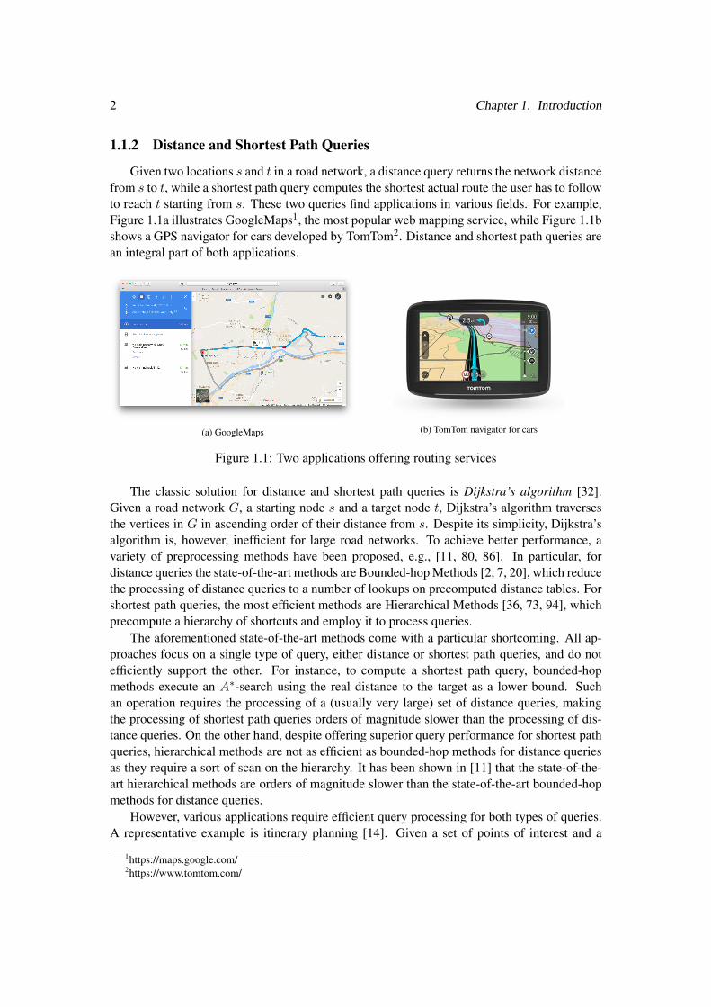
Given two locations s and t in a road network, a distance query returns the network distancefrom s to t, while a shortest path query computes the shortest actual route the user has to followto reach t starting from s. These two queries find applications in various fields. For example,Figure 1.1a illustrates GoogleMaps1, the most popular web mapping service, while Figure 1.1bshows a GPS navigator for cars developed by TomTom2. Distance and shortest path queries arean integral part of both applications.
(a) GoogleMaps (b) TomTom navigator for cars
Figure 1.1: Two applications offering routing services
The classic solution for distance and shortest path queries is Dijkstra’s algorithm [32].Given a road network G, a starting node s and a target node t, Dijkstra’s algorithm traversesthe vertices in G in ascending order of their distance from s. Despite its simplicity, Dijkstra’salgorithm is, however, inefficient for large road networks. To achieve better performance, avariety of preprocessing methods have been proposed, e.g., [11, 80, 86]. In particular, fordistance queries the state-of-the-art methods are Bounded-hop Methods [2, 7, 20], which reducethe processing of distance queries to a number of lookups on precomputed distance tables. Forshortest path queries, the most efficient methods are Hierarchical Methods [36, 73, 94], whichprecompute a hierarchy of shortcuts and employ it to process queries.
The aforementioned state-of-the-art methods come with a particular shortcoming. All ap-proaches focus on a single type of query, either distance or shortest path queries, and do notefficiently support the other. For instance, to compute a shortest path query, bounded-hopmethods execute an A⇤-search using the real distance to the target as a lower bound. Suchan operation requires the processing of a (usually very large) set of distance queries, makingthe processing of shortest path queries orders of magnitude slower than the processing of dis-tance queries. On the other hand, despite offering superior query performance for shortest pathqueries, hierarchical methods are not as efficient as bounded-hop methods for distance queriesas they require a sort of scan on the hierarchy. It has been shown in [11] that the state-of-the-art hierarchical methods are orders of magnitude slower than the state-of-the-art bounded-hopmethods for distance queries.
However, various applications require efficient query processing for both types of queries.A representative example is itinerary planning [14]. Given a set of points of interest and a
1https://maps.google.com/2https://www.tomtom.com/

1.1. Motivation and Problem Setting 3
time budget, itinerary planning computes one or more itineraries that visit as many points ofinterest as possible within the given time budget. During the planning phase, many distancequeries need to be answered between points of interest, and once valid combinations of pointsare found, the distinct paths connecting those points must be determined. In such scenarios,to achieve optimal performance, the maintenance of two separate structures is necessary. Thisleads to the first problem addressed in this thesis:
Problem 1. Existing solutions focus on one query type, either distance or shortest pathqueries, and do not efficiently support the other.
1.1.3 Alternative Routing
In many real-world scenarios, determining solely the shortest path is not enough. Mostcommercial route planning applications and navigation systems recommend alternative pathsthat might be longer than the shortest path but have other desirable properties (e.g., lower fuelconsumption), leaving the final decision to the user. Alternative routing is also very useful forthe transportation of goods using a fleet of vehicles, i.e., transportation of humanitarian aidthrough unsafe regions. By distributing the load into vehicles that follow different routes, theprobability that at least some of the goods will arrive at the destination safely can be increased.Another interesting scenario arises in emergency situations such as natural disasters and terror-ist attacks. To avoid panic and potential catastrophic collisions while dealing with the aftermathof such events, evacuation plans should include, apart from the shortest, alternative paths whichoverlap as little as possible.
Consider the scenario illustrated in Figure 1.2, which shows three distinct paths from loca-tion s to t in the city center of Bolzano. The solid/black line indicates the shortest path froms to t, whereas the dotted/red line indicates the next path in length order. Notice how similarthese two paths are. On the other hand, the green/dashed line indicates a third path which isclearly the longest but is significantly different from the shortest path. In practice, the pathscover very distant parts of the city’s road network. In applications like the ones discussed inthe previous paragraph, only the green/dashed path can be considered as a good and usefulalternative to the shortest path.
Figure 1.2: Illustration of alternative paths
Existing works for recommending alternative paths come with two important shortcomings.First, many approaches define alternative paths based on their similarity to the shortest path,

4 Chapter 1. Introduction
which may result in alternative paths being very similar to each other and, hence, of limitedinterest to the user. Second, most existing methods typically give no guarantees regarding thelength of the alternative paths. Naturally, the users have more interest in paths that are as shortas possible. This leads to the second problem addressed in this thesis:
Problem 2. There exist no solutions that compute k alternative paths that are as short aspossible and at the same time sufficiently dissimilar to each other.
1.2 Objectives and Contributions
The overall goal of this thesis is to propose efficient algorithms for route planning on roadnetworks. In particular, we study two different problems related to route planning: the efficientprocessing of distance and shortest path queries, and the computation of dissimilar yet shortalternative paths. In what follows, we summarize the technical contributions of this thesis.
1.2.1 ParDiSP Framework
We propose a Partition-based framework for Distance and Shortest Path queries (ParDiSP)that efficiently computes both types of queries. ParDiSP combines ideas from state-of-the-artapproaches in a novel way, thereby providing exceptional query times for both distance andshortest path queries. More specifically, ParDiSP partitions the road network into k componentsand precomputes auxiliary information. The precomputed information enables ParDiSP toprocesses distance queries as a bounded-hop method, i.e., by executing a number of table look-ups. For processing shortest path queries, ParDiSP utilizes the result of a distance query toidentify the subset of the road network that needs to be accessed to process the given query.Furthermore, in contrast to most existing methods, ParDiSP provides flexibility, i.e, the numberk of components can be used to adjust the trade-off between performance and space overhead.
In practice, ParDiSP exploits the properties of the road network partitioning to precomputeboth distance tables and graph structures. ParDiSP answers distance queries by combiningdistances from exactly three precomputed distance tables. Shortest path queries are decom-posed into three segments, which can be computed in parallel by accessing only a small part ofthe original road network. To compute the longest of the three segments, ParDiSP employs astate-of-the-art hierarchical method over a precomputed part of the road network. We evaluateParDiSP in terms of performance and preprocessing cost and show that: ParDiSP outperformstwo state-of-the-art solutions for shortest path queries; it is comparable to the state-of-the-artfor distance queries; and, for mixed query loads containing both distance and shortest pathqueries, ParDiSP outperforms a combination of the best methods for each query type, while itsspace requirements are significantly smaller.
1.2.2 k-SPwLO Queries
We propose a novel definition of alternative paths. More specifically, we recommend aset of k paths (including the shortest path) such that every path in the result is (a) sufficientlydissimilar to all shorter paths in the set and (b) as short as possible. We formalize this formof alternative routing as the k-Shortest Paths with Limited Overlap (k-SPwLO) problem. We

1.3. Publications 5
also present three algorithms to evaluate k-SPwLO queries. First, the baseline algorithm BSLbuilds upon the computation of the K-shortest paths. Second, OnePass traverses the roadnetwork once expanding every path from the source that qualifies the similarity constraint.Third, MultiPass extends and improves OnePass by employing an additional pruning criterionand processes queries by traversing the network k�1 times. In an extensive experimentalevaluation we show that MultiPass is the fastest algorithm for processing k-SPwLO queriesoutperforming both BSL and OnePass.
Despite MultiPass being the fastest exact solution for processing k-SPwLO queries, thealgorithm is not practical for large road networks. Therefore, we also propose two heuristicalgorithms3 that trade result quality for efficiency. Our first heuristic algorithm, OnePass+,employs the pruning power of MultiPass, but, similar to OnePass, traverses the road networkonly once. The second heuristic algorithm, ESX, reduces the search for alternative paths toa set of shortest path queries by incrementally removing edges from the road network. In theexperimental evaluation, we compare the heuristic algorithms with MultiPass, the most efficientexact solution, in terms of performance and result quality. OnePass+ runs significantly fasterthan MultiPass and its result is close to the exact solution, while ESX is faster than OnePass+
(though slightly less accurate) and it scales for large road networks and large values of k.
1.2.3 MoTrIS Framework
Finally, we present MoTrIS, a Multimodal Transport Information System, which integratestwo of the algorithm presented in this thesis: ParDiSP for processing distance and shortest pathqueries and ESX to recommend alternative routes. Apart from route planning on road net-works, MoTrIS tackles the challenge of combining different types of networks, i.e., road andtransportation networks, into a single multimodal network. Developers can create customizedrouting services over specific regions and with specific transportation modes. MoTrIS also pro-vides a public API which enables developers to submit queries and integrate the functionalitydirectly into their applications. We also show that MoTrIS is highly extensible. New algorithmscan be easily integrated to support the processing of more types of routing queries on road andmultimodal transportation networks.
1.3 Publications
The results presented in this thesis have been published at the following conferences:
- T. Chondrogiannis and J. Gamper, Exploring Graph Partitioning for Shortest Path Querieson Road Networks, In Proceedings of the 26th Grundlagen von Datenbanken (GvDB’14),pages 71-76, 2014
- T. Chondrogiannis, P. Bouros, J. Gamper and U. Leser, Alternative Routing: k-Shortest Pathswith Limited Overlap, In Proceedings of the 23rd ACM SIGSPATIAL International Confer-ence on Advances in Geographic Information Systems (GIS’15), pages 68:1-68:4, 2015
3In [18] the term ”approximate algorithms” was used instead of ”heuristic algorithms”. Since our algorithmscome with no error guarantees, we changed the terminology as the term ”heuristic” is more accurate.
6 Chapter 1. Introduction
- T. Chondrogiannis and J. Gamper, ParDiSP: A Partition-based Framework for Distance andShortest Path Queries on Road Networks, In Proceedings of the 17th IEEE InternationalConference on Mobile Data Management (MDM’16), pages 242-251, 2016
- T. Chondrogiannis, J. Gamper, R. Cavaliere and P. Ohnewein, MoTrIS: A Framework forRoute Planning on Multimodal Transportation Networks, In Proceedings of the 24th ACMSIGSPATIAL International Conference on Advances in Geographic Information Systems(GIS’16), pages 82:1-82:4, 2016
- T. Chondrogiannis, P. Bouros, J. Gamper and U. Leser, Exact and Approximate Algorithmsfor Finding k-Shortest Paths with Limited Overlap, In Proceedings of the 20th InternationalConference on Extending Database Technology (EDBT’17), pages 414-425, 2017
1.4 Thesis Organization
Chapter 2. This chapter discusses related research work in the areas of distance and shortestpath query processing as well as alternative routing. In addition, since our prototype system ispart of the thesis, we review state-of-the-art implementations with similar functionalities.
Chapter 3. This chapter presents the Partition-based Framework for Distance and Short-est Path Queries (ParDiSP) on road networks, which combines ideas from state-of-the-art ap-proaches for distance and shortest path processing in a novel way.
Chapter 4. In this chapter, we first introduce the k-SPwLO query for alternative routingon road networks. We also propose and evaluate three algorithms for processing k-SPwLOqueries which examine the paths from the source node in increasing order of their length andprogressively construct the result set.
Chapter 5. In this chapter, we study heuristics to compute k-SPwLO queries and we proposetwo heuristic algorithms which trade accuracy for efficiency. We also present the results of anextensive experimental evaluation, comparing the heuristic algorithms with the most efficientexact solution, both in terms of performance and result quality.
Chapter 6. This chapter presents MoTrIS, our service-oriented platform which integrates ouralgorithms. We describe the system architecture and we present use-cases which demonstratethe main functionalities of the platform.
Chapter 7. This chapter summarizes the achieved results and points out some interestingdirections for future research work.

CHAPTER 2
Related Work
In this chapter, we discuss related research work, which we divide in four parts. The firstpart in Section 2.1 focuses on state-of-the-art preprocessing-based methods for distance andshortest path query processing on static road networks. The second part in Section 2.2 reviewsalgorithms for computing alternative routes on road networks. The third part in Section 2.3discusses the problem of route planning on multimodal transportation networks, i.e., usingdifferent transportation modes. Finally, Section 2.4 provides an overview of popular opensource and commercial routing applications and systems.
7

8 Chapter 2. Related Work
2.1 Distance and Shortest Path Queries on Road Networks
In the last twenty years, the processing of spatial network queries has attracted consider-able interest and a variety of methods to process such queries have been proposed. In [65], astorage model for spatial network databases has been proposed along with algorithms for var-ious spatial network queries, i.e., k-nearest neighbor (kNN) queries, range queries and closestpair queries. For nearest neighbor and kNN queries in particular, various approaches have beenproposed [23, 30, 49, 65, 72]. Many algorithms have also been proposed for processing vari-ants of nearest neighbor queries, i.e., aggregate nearest neighbor queries [64, 90], group nearestneighbor queries [63] and reverse nearest neighbor queries [91].
Among spatial network queries, distance and shortest path queries are the most fundamentaland among the most popular queries. The classical solution for processing such queries isDijkstra’s algorithm [32]. Given a road network G = (N,E), a starting node s and a targetnode t, Dijkstra’s algorithm traverses the nodes in G in ascending order of their distancesfrom s. In practice, Dijkstra’s algorithm works as follows: each node is associated with atentative distance which is initially set to +1 for all nodes, apart from s for which the tentativedistance is set to 0. Starting from s, the algorithm expands all outgoing edges of s, checkswhether by traversing the current edge the distance to the adjacent node is lower than the currenttentative distance and, if necessary, updates the tentative distances of the adjacent nodes. Onceall outgoing edges are visited, the node is called expanded. At each iteration, the node withthe smallest tentative distance that has not yet been expanded is examined. The expansionterminates either when the target node t is encountered or there are no more nodes to expand,in which case there is no path connecting nodes s and t.
A simple improvement to Dijkstra’s algorithm is to perform a bidirectional search [67], i.e.,to execute Dijkstra’s algorithm simultaneously from the source s and backwards from the targett. The search stops when a valid meeting point of the two shortest path trees is determined.Bidirectional search can improve the execution time of Dijkstra’s algorithm by a factor of two.However the improvement is not sufficient; like Dijkstra’s algorithm, bidirectional search isalso impractical for large road networks.
In order to make distance and shortest path queries scalable for large road networks, avariety of preprocessing based methods have been proposed [11, 80]. Such methods aim atprecomputing auxiliary information offline, inflicting a relatively high one time cost, and em-ploy the precomputed information in order to reduce the query processing time. Dependingon the precomputed information and the way each method utilizes it, we can classify exist-ing methods into five main categories: Speed-up methods, Spatial Coherence-based methods,Bounded-hop methods, Hierarchical methods, and Partition-based methods. In what follows,we present the most important methods in each category.
2.1.1 Speed-up Methods
Speed-up or goal-directed methods employ a modified version of Dijkstra’s algorithm alongwith heuristics to prioritize the expansion of nodes that are closer to the target. As Dijkstra’salgorithm has to visit a very large part of the road network, speed-up methods aim at reducingthe part of the network that the search algorithm has to expand.
A⇤-search [40] is a classic goal-directed algorithm which employs lower bounds to reducethe search space and speed-up shortest path query processing. The lower bound is determined
2.1. Distance and Shortest Path Queries on Road Networks 9
by employing a heuristic function h : N � < on the nodes of the input road network. Thealgorithm then employs a modified version of Dijkstra’s algorithm setting the priority of eachnode n to dist(s, n) + h(n, t) causing the nodes that are closer to the target to be visitedfirst. Naturally, the tighter the lower bound, the less the nodes that the search algorithm isgoing to visit. For example, in the case where we have the tightest possible lower bounds,hence h(n, t) = dist(n, t), then, for any shortest path query from s to t, A⇤-search visits onlynodes on the shortest path from s to t. Like Dijkstra’s algorithm, A⇤-search can also run in abidirectional fashion too [38].
Common heuristics employed by A⇤-search on road networks is the Euclidean distanceand the Manhattan distance. However, such heuristics fail to take into consideration the struc-ture of the road network and, therefore, in many cases, the improvement is minimal. An al-ternative way to obtain lower bounds is to employ landmarks. Landmark-based A⇤-search(ALT) [38] precomputes distances from all nodes of the road network to a small subset ofnodes, called landmarks. During the execution of a shortest path query from a source node sto a target node t, the lower bound of the distance from a node n visited by the algorithm tot is computed by employing the triangle inequality. More precisely, for any landmark l, wehave dist(n, t) � dist(n, l)� dist(t, l) and dist(n, t) � dist(l, t)� dist(l, n). For each noden the algorithm always picks the tightest possible lower bound among all bounds computedusing different landmarks. Apparently, the quality of the lower bounds depends heavily on theselection of landmarks during preprocessing; several techniques for selecting lanmarks havebeen proposed [68].
The ALT algorithm has been improved by incorporating reach labels [39] resulting in theReach-based ALT (REAL) [37] algorithm. The reach of a node n is defined as R
st
(n) =
min{dist(s, n), dist(n, t)}. The shortest path search can be pruned at nodes with a reachtoo small to get to the source or the target. Although reach values are determined during thepreprocessing phase, computing exact reaches requires the computation of the all-pairs shortestpaths; such an operation is prohibitively expensive. The result of the query is correct even ifthe reach of a node represents an upper bound. Such upper bounds can be obtained much fasterby computing partial shortest path trees.
Despite offering a significant improvement to Dijkstra’s algorithm, speed-up methods arenot efficient enough for large road networks. Speed-up methods are two to three orders ofmagnitude slower than state-of-the-art methods for distance and shortest path queries [11]. Incontrast to state-of-the-art methods though, speed-up methods are usually space efficient, i.e.,have much lower memory requirements.
2.1.2 Spatial Coherence-based Methods
Spatial coherence-based methods exploit the property of road networks that shortest pathsare often spatially coherent, i.e., many shortest paths between different pairs of nodes sharecommon parts. To illustrate the concept of spatial coherence, let us consider four locations s,s0, t and t0 on a road network. If s is close to s0 and t is close to t0, the shortest path from sto t is more likely to share nodes with the shortest path from s0 to t0. Spatial coherence-basedmethods precompute the all-pair shortest paths and employ some data structure to index thepaths and answer queries.
Spatially Induced Linkage Cognizance (SILC) [72, 74] precomputes and indexes the short-est paths between all pairs of nodes using a quad-tree [34]. For each node n of the input road

10 Chapter 2. Related Work
network, SILC computes the shortest paths from n to all the other nodes of the road network.Then SILC imposes a grid on the road network and splits the grid into areas such that: (i) everyarea contains exactly one neighbor of n and (ii) the shortest path from n to any node insidean area passes through the neighbor of n assigned in the same area. Hence, given a shortestpath query from a source node s to a target node t, starting from s, SILC can identify which ofthe neighbors of the node examined at each iteration lies on the shortest path to t. It has beenshown that every lookup of SILC requires O(log n), while the number of lookups depends onthe number of nodes on the shortest path.
Path-Coherent Pairs Decomposition (PCPD) [77] imposes a grid over the road networksand precomputes the shortest paths between all pairs of nodes, like SILC. Then, PCPD stores allpaths in a concise format called path coherent pairs. A path coherent pair is a triple hA,B, ni,where A and B are two disjoint square regions of the grid and n is a node of the road networksuch that all shortest paths p(s!t) from some node s located inside A to some node t locatedinside B pass through node n. Similar to SILC, in order for PCPD to retrieve a shortest path,it requires linear time to the size of the path, i.e., the same number of lookups as the numberof nodes on the path. Each lookup using the aforementioned path coherent pairs scheme costsO(m) where m is the number of unique path coherent pairs computed during preprocessing.
Spatial coherence is also employed by distance oracles, an efficient approach for approxi-mate distance query processing. In [82], the authors propose an (1+✏, 0)-approximate distanceoracle, a multi-level approach which answers approximate distance queries in almost constanttime while inflicting relatively low space overhead. Another method for approximate distancequery processing is the ✏-approximate distance oracle presented in [76]. The oracle requiresO(n/✏2) space and retrieves the approximate network distance in O(log n) time using a B-tree. Although very efficient, methods based on distance oracles cannot answer exact distancequeries and approximate distance query processing is out of the scope of this thesis.
The main shortcoming of spatial coherence-based methods is that they incur significant pre-processing time and space overhead. In particular, although SILC and PCDP offer exceptionalquery times for both distance and shortest path queries, their space overhead is exponential tothe number of nodes [86]. Both methods have prohibitively high memory requirements evenwhen applied on road networks with less than a million nodes. Hence, spatial coherence-basedmethods are clearly not practical for large road networks with several millions of nodes.
2.1.3 Bounded-hop Methods
Bounded-hop methods precompute and store distances between selected pairs of nodes intoa set of distance tables. The distance between any pair of nodes is computed by accessing onlythe precomputed distance tables, and then the shortest path is retrieved by running an A⇤-searchfrom the source to the target using the exact distance as a lower bound; hence, the retrieval ofthe shortest path is linear to the size (number of nodes) of the path.
The 2-hop cover [20] is an early theoretical distance labeling scheme which works as fol-lows. During preprocessing, every node n of the road network is assigned with a set of labelsL(n) containing distances to selected nodes such that for any pair of nodes s and t, L(s)\L(t)contains at least one node on the shortest path from s to t. This method ensures that the shortestpath from s to t is covered by a node in L(s) \ L(t), i.e., the distance from s to t can be foundby combining only distances in L(s) and L(t). The 2-hop cover is the the minimum set ofnodes that can be used as labels to compute the shortest paths between any pair of nodes on the

2.1. Distance and Shortest Path Queries on Road Networks 11
road network. However, the computation of the 2-hop cover requires the computation of theall-pair shortest paths, thus is prohibitively expensive.
Hub Labeling (HL) [2, 3], is a labeling technique for distance queries on road networksbased on the theory of 2-hop cover. Each node is associated with a label L(n) which containsdistances to a set of nodes, i.e., the hubs of n. HL guarantees that the cover property of the2-hop cover is obeyed; hence, any distance dist(s, t) can be determined in linear time bycombining exactly two distance tables, i.e., L(s) and L(t). Apparently, the performance ofdistance queries depends on the size of the distance tables. Even though HL does not guaranteethat the size of the distance tables is minimum, the proposed label selection strategy leads tosmall distance tables and, therefore, exceptional query times.
Another popular bounded-hop technique is Transit Node Routing [12, 8]. In contrast to HL,TNR combines three distance tables to compute the distance between two nodes. Given a roadnetwork G = (N,E), during preprocessing TNR selects a small set T ✓ N of transit nodesand computes all pairwise distances between them. Then, the algorithm assigns to each noden 2 N a set of access nodes A(n) ✓ T and precomputes the distances from and to every accessnode in the assigned set. To determine the access nodes, the algorithm imposes a grid on theroad networks such that each grid cell contains at most one node. TNR chooses as access nodesof a given node, the nodes that are located inside neighboring grid cells. The result for a givendistance query q(s, t) is dist(s, t) = min{d(s, a
s
) + d(as
, at
) + d(at
, t)}, where as
2 A(s)and a
t
2 A(t).
Pruned Highway Labeling (PHL) [7] introduces a cost efficient preprocessing method toselect labels. Although a pure bounded-hop technique, PHL combines features from differ-ent aspects in the literature. In particular, PHL repeatedly separates input road networks byshortest paths, and then stores distances from nodes to the shortest paths. This is an idea alsoemployed by distance oracles for approximate distance query procesing [82]. PHL also utilizesthe concept of highways [73, 78] in order to compute the set of labels assigned to each node.During preprocessing, PHL computes labels such that any shortest path from a node s to a nodet can be expressed as a sequence of three paths hp(s, u), p(u, v), p(v, t)i, where path p(u, v)is a highway; distance dist(u, v) is precomputed while u and v are stored as labels of s and talong with their respective distances from s and t.
Bounded-hop methods and, in particular, HL [3], are the most efficient approaches for pro-cessing distance queries. Experiments presented in [11] have shown that HL requires less thana microsecond to process distance queries even on continental road networks. In comparisonto other approaches, HL is eight orders of magnitude faster than Dijkstra’s algorithm and fivetimes faster than TNR. However, HL requires a lot of preprocessing time and memory. Interms of performance, the method closest to HL is PHL [7]. PHL answers distance queriesapproximately in one microsecond, i.e., it is slightly slower than HL. However, PHL requiressignificantly less memory and preprocessing time than HL.
Although very efficient for distance queries, bounded-hop methods are not as efficient forshortest path queries. As we mentioned before, to retrieve the shortest path, bounded-hopmethods execute an A⇤-search from the source to the target using the real distance to the targetas a lower bound. Processing a shortest path query is essentially equivalent to processing a(large) set of distance queries, which depends heavily on the network structure and the lengthof the shortest path.

12 Chapter 2. Related Work
2.1.4 Hierarchical Methods
Hierarchical methods impose a hierarchical structure on the road network and processqueries by running a bidirectional search over the precomputed structure. The hierarchicalstructure usually consists of shortcuts which aim at abstracting the main arteries of the roadnetwork. By traversing the hierarchy instead of the original road network, the search space forcomputing shortest path queries is significantly reduced.
Highway Hierarchies (HH) [73] are based on the following observation. Certain edges ofthe road network, i.e., the highway edges, tend to be on many shortest paths where the sourceand the target are far apart. HH employs two sub-routines to build a hierarchy of shortcuts onthe road network. Node reduction introduces shortcuts to bypass nodes of low degree, i.e., oneor two. Edge reduction adds shortcuts to bypass non-highway edges. To identify non-highwayedges, HH performs a local check for each edge of the road network. To process queries, HHemploys a modified version of bidirectional search [67], which avoids expanding most of thenon-highway edges.
Contraction Hierarchies (CH) [36] is a direct successor of HH, which organizes the nodeson a road network into a hierarchy, based on their relative importance. During preprocessing,CH determines the importance of each node by employing a set of heuristics, generates a nodeorder and contracts each node on the road network following the precomputed order. The resultof the contraction process is the construction of a multi-level hierarchical structure of shortcuts.Like HH, to process shortest path queries a modified bidirectional search is executed over thehierarchical structure. At each step, the search algorithm visits nodes that are on the same or ahigher level than the last expanded node.
Arterial Hierarchy (AH) [94] is a method inspired by CH, which precomputes shortcutsby imposing a grid on the road network. AH organizes the nodes of the road network intolevels such that during query processing the network traversal will always visit a node froma higher level than the current one. AH is the only hierarchical method which comes withtheoretical guarantees regarding the space overhead and the query processing time. AH buildsthe shortcut hierarchy in a way that it guarantees the levels of the hierarchy will be O(log n).As a consequence, AH provides a time complexity of O(log n) for processing queries.
Hierarchical methods and, in particular, AH and CH are the most efficient methods forshortest path queries. In [94] it is shown that AH outperforms CH in both distance and short-est path queries at the cost of extra space and preprocessing time. Despite offering superiorquery performance for shortest path queries though, hierarchical methods are not as efficientas bounded-hop methods for distance queries as they require a sort of scan on the hierarchy. Ithas been shown in [11] that CH is approximately three orders of magnitude slower than HL fordistance queries.
2.1.5 Partition-based Methods
Partition-based methods first partition the input road network into a number of components.For this purpose, a third-party partitioning method is usually employed, which splits the nodesinto balanced components while attempting to minimize the number of connecting edges, i.e.,edges between border nodes of neighboring components. By employing the inherent propertiesof the partition, shortcuts and/or distance tables are precomputed to boost query processing.Most partition-based methods share some characteristics with methods from other categories,
2.1. Distance and Shortest Path Queries on Road Networks 13
i.e., speed-up, bounded-hop or hierarchical methods.Precomputed Cluster Distances (PCD) [60] is a speed-up technique which partitions the
input road network into components, precomputes the distances between all pairs of compo-nents and uses these distances to compute lower bounds. More specifically, PCD first partitionsthe road network into k components {C1 . . . C
k
}. During the preprocessing phase, the algo-rithm computes the distances between all pairs of components. The distance between twocomponents C
i
and Cj
is defined as the minimum distance between two nodes ni
2 Ci
andnj
2 Cj
. For computing a shortest path query from a source node s 2 CS
to a target nodet 2 C
t
, PCD executes an A⇤-search employing the distance between components to com-pute lower bounds. For any visited node n 2 C
n
, a valid lower bound on its distance to t isdist(s, n) + dist(C
n
, Ct
) + dist(bt
, t), where bt
is the border node of Ct
that is closest to t.Arc Flags [48] partitions the road network into k components and assigns to each edge of
the road network a vector of k bits (arc flags). The ith bit of the vector is set if the edge lies ona shortest path to some node of component i. While processing a shortest path query from s tot, the search algorithm prunes edges which do not have the bit set for the component containingtarget t. The arc flags for a component i are computed by growing a backward shortest pathtree from each border node (of component i), setting the ith flag for all edges on the tree.
Hierarchical Encoded Path Views (HEPV) [45] is a hierarchical partition-based methodwhich employs Spatial Partition Clustering (SPC) [42], a custom partitioning algorithm for roadnetworks. First, HEPV partitions the input road network into components using SPC. Duringthe preprocessing phase, the shortest path between every pair of border nodes is computed.HEPV stores and maintains the entire shortest path between two border nodes instead of themere distance, in the form of a path view. Next, an auxiliary graph is created, which consistsof several partial graphs. Each partial graph keeps all the path views which store shortest pathsbetween the border nodes of its associated component. Next, HEPV partitions the resultingauxiliary graph into subgraphs and computes shortest paths in the same fashion in order topopulate the next level of the hierarchy. The process continues until the top auxiliary graphis sufficiently small. To retrieve the shortest path between two nodes, HEPV retrieves andcombines the partial paths from the appropriate components, usually from two different levelsof the hierarchy. HiTi Graphs [46] also employ a similar approach to HEPV.
Customizable Route Planning (CRP) [26] partitions the road network into components andprecomputes distances between border nodes in each component. To partition the input roadnetwork, CRP employs PUNCH [27], another graph partitioning algorithm tailored to roadnetworks. To process queries, a modified bidirectional search algorithm is employed, whichexpands only the shortcuts and the edges in the source and the target component. In contrast toHEPV and HiTi, CRP stores only the distances between border nodes. Hence, for each shortcuton the shortest path, CRP has to retrieve the path from the original road network. Since theprecomputed information is limited to one distance table per node, the memory requirementsof CRP are quite low. Hence, CRP is able to handle various arbitrary metrics by precomputingmore distance tables per node.
Finally, G-tree [93], PTree [84] and G⇤-tree [5] use the same hierarchical partition-basedstructure for processing spatial network queries. All these methods partition the road networkrecursively and construct a hierarchy of components. For components at the lowest-level thedistances between every node and all border nodes are stored, whereas for the other componentsonly the distances between pairs of border nodes are stored. All approaches handle distance

14 Chapter 2. Related Work
queries using precomputed distance tables. In addition, G-Tree uses the structure to computenearest neighbor queries, PTree employs dynamic programming to retrieve shortest paths, andG⇤-tree [93] employs a different partitioning strategy to process k-closest pairs queries.
2.2 Alternative Routing on Road Networks
A first take on providing alternative routes on road networks is to solve the K-shortest(simple) paths problem. It has been shown that Yen’s algorithm, initially proposed in [89] andfurther optimized in [41, 59], is the most efficient algorithm for computing the K�shortestpaths. The main idea behind Yen’s algorithm is that, given a source node s and a target nodet, in order to compute the Kth shortest path from s to t we must have already computed thefirst K�1 shortest paths. Hence, the first step of Yen’s algorithm is to employ any traditionalalgorithm to compute the shortest path from s to t, e.g., Dijkstra’s algorithm. By analyzingthe shortest path, a candidate path will be generated for each node of the shortest path, andthe shortest among the candidate paths will be chosen as the next shortest path. The processcontinues until the Kth shortest path has been determined. In practice , the K�shortest pathscannot be employed for alternative routing. In most cases the K�shortest paths share largestretches and, therefore, they are of little practical value as alternative routes.
In [44], the authors propose an algorithm which directly extends Yen’s algorithm [89] tocompute k-dissimilar paths on road networks. Given a source node s and target node t, a lengthlimit x and a similarity threshold y, the goal is to incrementally compute k paths, the lengthof which does not exceed x and their pairwise similarity does not exceed y. The similaritybetween two paths is defined based on the length of their shared edges. The shortest pathfrom s to t is always included in the final result set. At each round, the algorithm computes aset of candidates, selects the most dissimilar path to the previously computed ones as the topcandidate and, if the candidate path satisfies the x, y constraints, it is added to the result set.The algorithm terminates when k valid paths have been found. Although pairwise dissimilarityis guaranteed, the algorithm does not aim at minimizing the length of the recommended paths.
In what follows, we describe different approaches presented in the bibliography on how togenerate alternative paths.
2.2.1 Penalty-based Methods
Penalty-based methods focus on the process of generating a set of paths different from theshortest path without, however, providing a formal definition of alternative routing. The mainidea of penalty-based methods is to compute the shortest path and then update the road networkby adding a penalty on the weights of the edges that lie on the shortest path. For example, in [6]the authors propose a method which doubles the weight of each edge that lies on the shortestpath. The alternative paths are computed by repeatedly running a shortest path algorithm, suchas Dijkstra’s algorithm, on the input road network, each time with the updated weights. Asimilar approach is adopted by [52] where the penalty is computed in terms of both the pathoverlap and the total turning cost, i.e., how many times the user has to switch between roadswhen following a path.
The main shortcoming of penalty-based methods is that there is no intuition behind thevalue of the penalty applied before each iteration. In general, using a large penalty would

2.2. Alternative Routing on Road Networks 15
result in dissimilar but possibly very long alternative paths. On the other hand, using a smallpenalty would require the algorithm to perform more iterations in order to find the desiredresult. Even so, penalty-based methods cannot provide a formal result set and, hence, theirefficiency depends upon the user’s choice of the penalty.
2.2.2 Candidate Set-based Methods
Another approach for alternative routing is to first compute a large set of candidate paths.Then, during a post-processing step, we examine the candidates with respect to a number ofconstraints (e.g., their length or the nodes they cross) and determine the final result set. Forexample, the Plateaux method [1] aims at computing paths that cross different highways of theroad network. Since highways rarely overlap, the produced paths are dissimilar. The problemand the proposed method in [1] were revisited and formally defined later in [9], which intro-duces the concept of alternative graphs having the same functionality as the plateaus, and werefurther improved in [66].
In [4], the authors use the set of single-via paths as their candidate set to compute alternativepaths. The proposed method first selects a subset of the network nodes called via-nodes, i.e.,all nodes of the road network apart from s and t. Then, it computes a single-via path for eachvia-node v by concatenating the shortest path from source s to v and the shortest path from vto target t. Each single-via path is compared to the shortest path based on a set of objectiveuser-defined criteria, i.e., excess length, local optimality and stretch. The single-via paths thatsatisfy all of the user-defined criteria are considered alternative paths. Optimizations for thismethod were recently presented in [56].
The main shortcoming of methods based on candidate sets is that none of the proposedmethods tackles the problem of computing multiple alternative paths dissimilar to each other.For example, the Plateaux method requires the existence of highways to recommend dissimilaralternative paths. However, in many real-world scenarios, i.e., within cities, the presence ofhighways is not always guaranteed. With regard to the method proposed in [4] where multiplesingle-via paths may be selected as alternative paths, their similarity only to the shortest pathis considered. Hence, the recommended paths may be very similar to each other. In Chapter 5we extend the method of [4] and propose the SVP+ algorithm, which builds upon the conceptof single-via paths and computes alternative paths dissimilar to each other.
2.2.3 Historical Data-based Methods
Historical data-based methods analyze historical information in order to extract informa-tion about the road network and provide more robust route planning services. A commonapproach is to analyze historical traffic information to compute traffic tolerant paths over time-dependent road networks [29, 51, 70, 88]. For alternative routing in particular, the k traffic-tolerant paths (TTP) problem [51] takes an s�t pair and historic traffic information as input,and returns k paths that minimize the aggregate (historic) travel time. In contrast to our workthough, TTP computes alternative paths without taking into consideration the similarity of theresult paths. Furthermore, similar to all historical data-based methods, TTP relies on the avail-ability of historical traffic information in order to compute alternative paths. In scenarios wheresuch information is not available, TPP cannot be applied.

16 Chapter 2. Related Work
Other historical data-based methods analyze and mine trajectory data in order to extractpopular routes [16, 17, 54, 81, 85, 92]. The main idea backing these methods is that expe-rienced drivers tend to follow routes based on their own preferences and/or their knowledgeabout the traffic conditions in a particular area. By mining trajectory data, useful informationcan be obtained and used by recommender systems in order to provide more reliable results.However, trajectory-based methods compute routes based on trajectories collected over a pe-riod of time under normal circumstances. Therefore, the number of routes that can be obtainedby using solely trajectory data is limited. Moreover, similar to historical traffic data for TPP,the availability of quality trajectory data is not always guaranteed.
2.2.4 Other Methods
Apart from the methods we described above, which define alternative routes using pathsimilarity, there are also other methods that define alternative routes in a different way. In [87],alternative shortest paths using edge avoidance are introduced. Given the shortest path p(s!t)and an edge e on p, the alternative path is the shortest path from s to t which avoids edge e.To compute alternative paths, the authors combine the concepts of distance oracles [75] anddistance sensitivity oracles [13] and propose iSPQF. The shortest path between every pair ofnodes avoiding each edge is precomputed and stored in a quadtree-based data structure inspiredby [72]. Given a road network G(N,E), iSPQF structure stores |N |2 quadtrees in total (|N |quadtrees per node). Alternative path queries are computed in almost constant time. Also,the authors show that by merging the quadtrees a worst case space complexity of O(n1.5
) isachieved. Although very efficient, iSPQF is limited to computing only one alternative routeinstead of a set.
Finally, the task of alternative routing can also be based on the pareto-optimal paths or theroute skyline query for multi-criteria networks [25, 50, 58, 61, 79]. A path p is part of thepareto-optimal set or the route skyline P if p is not dominated by another path p0 2 P . Path pdominates p0 iff p is no worse than p0 in all criteria/dimensions of the network (e.g., distance,travel time, gas consumption) and strictly better than p0 in at least one of those criteria. Thepareto-optimal paths or the route skyline can be directly seen as alternative routes to movefrom source node s to target node t or can be further examined in a post-processing phase toprovide the final alternative paths. Nevertheless, our definition of alternative routing is not amulti-criteria problem and the recommended paths by k-SPwLO cannot be obtained by firstcomputing the pareto-optimal path set.
2.3 Multimodal Networks
The multimodal route planning problem seeks journeys combining schedule-based trans-portation (e.g., buses and trains) with unrestricted modes (e.g., walking and driving). Thisproblem is significantly harder than its individual components as it involves the combination oftwo or more networks, usually of different types, into a single multimodal network.
A general approach to construct a multimodal network requires to build an individual net-work for each transportation mode. However, while a pedestrian network can be modeled usinga static graph, i.e., the weights of edges do not change over time, public transportation networksare usually modeled as schedule-based networks, a special case of time-dependent networks. In

2.4. Routing Applications and Systems 17
time-dependent networks, the weight of an edge varies depending on the time of the day that itis crossed. Each edge is associated with a time-dependent function which takes as an argumenta timestamp t and returns the weight of the edge on time t. For schedule-based networks inparticular, the function is used to query the schedule of the given transportation mode.
Pyrga et al. [69] summarize two different models for modeling timetable information. Thetime-expanded model constructs the time-expanded digraph in which every node corresponds toa specific time event (departure or arrival) at a station and edges between nodes represent eitherelementary connections between the two events (i.e., served by a train that does not stop in-between) or waiting within a station. The time-dependent model constructs the time-dependentdigraph in which every node represents a station and two nodes are connected by an edge if thecorresponding stations are connected by an elementary connection. The costs on the edges areassigned ”on-the-fly”, i.e., the cost of an edge depends on the time in which the particular edgewill be expanded by the shortest-path algorithm to answer the query.
After each individual network graph is constructed, all individual networks are merged intoa single multimodal network by adding link edges between nodes of different networks. Forexample, in order to combine a pedestrian network and a bus network, we add links so thatevery node of the bus network is connected to some node of the pedestrian network. Typicalexamples [28, 62] model walking as a static graph and public transportation networks using therealistic time-dependent model.
Various approaches for route planning [28, 31] and alternative routing [10, 24] on multi-modal networks have been proposed. A direct solution to compute the shortest path betweentwo nodes in a multimodal network though is to employ a modified version of Dijkstra’s al-gorithm [32]. Since the multimodal network contains both edges with a fixed weight andtime-dependent edges, the weight of each edge is determined ”on-the-fly” based on its type.Also, when the search algorithm switches from the road (static) network to a transportation(time-dependent) network, the waiting time, i.e., the time between the arrival of the user at astop and the departure time of the vehicle from the stop, has to be considered.
2.4 Routing Applications and Systems
Numerous systems that offer route planning services have been proposed in the last decade.OSRM/MoNav [55] obtains data from OpenStreetMap and allows the processing of distanceand shortest path queries on road networks. To optimize query processing OSRM/MoNav em-ploys CH [36]. Graphhopper 1 is a similar service-oriented open-source system which alsoemploys CH. TransDec [29] is a real-world data-driven framework which obtains data fromsensors and analyzes the traffic conditions on the road network. In addition, it stores and an-alyzes historical trajectory data to improve the quality of the results. In a similar context,CrowdPlanner [81] also employs historical information and recommends routes by taking intoconsideration the preferences of the users. For transportation networks, Graphast [57] is aframework which enables processing time-dependent spatio-temporal network queries [22].Finally, ISOGA [43] enables the computation of isochrones on multimodal networks for reach-ability analysis.
1https://graphhopper.com

18 Chapter 2. Related Work
2.5 Summary
To sum up, there has been a lot of research work in the area of route planning. In partic-ular, a huge variety of preprocessing-based methods for computing distance and shortest pathqueries on road networks have been proposed. State-of-the-art methods for distance queriesoffer exceptional query times, but they do not provide any efficient retrieval mechanism forthe shortest path. In contrast, state-of-the-art methods for shortest path queries show relativelypoor performance for distance queries. However, many applications require efficient queryprocessing for both types of queries. Our ParDiSP approach (cf. Chapter 3) aims at filling thisgap in existing research as it provides exceptional query times for both distance and shortestpath queries.
In the area of alternative routing, existing literature has approached the computation ofalternative paths from different perspectives. Most current approaches either do not propose aformal result set and, hence, provide no guarantees regarding the quality of the recommendedpaths, or they propose alternative paths based solely on their individual similarity to the shortestpath, which results in alternative paths that are very similar to each other. In contrast to theseapproaches, our k-SPwLO query (cf. Chapter 4) aims at computing paths that are sufficientlydissimilar to each other and as short as possible.
CHAPTER 3
Partition-based Shortest Path Query Processing
Our preliminary investigation in [19] showed that in order to boost distance and shortestpath query processing using a single approach is not enough. Bounded-hop methods are ex-ceptionally fast for distance queries. Reducing the evaluation of distance queries to a numberof lookups is clearly the best approach. For shortest path queries, we observed that in order tooptimize the evaluation, the utilization of some form of shortcuts is required. It has been shownin [86] that the most efficient way to generate shortcuts is to follow a hierarchical approach.
In this chapter, we present the Partition-based framework for Distance and Shortest Pathqueries (ParDiSP) on road networks. ParDiSP combines ideas from both bounded-hop and hi-erarchical methods in a novel way, taking the best of both worlds, and efficiently supports bothdistance and shortest path queries. During preprocessing, ParDiSP precomputes the distancesbetween any node in a component and the border nodes of the same component, the pairwisedistances between all border nodes, and the union of the shortest paths between all bordernodes. ParDiSP answers distance queries by combining distances from exactly three precom-puted distance tables. For shortest path queries, the information in the distance tables allowsto identify two border nodes that are traversed by the shortest path, thereby decomposing thepath into three segments which can be computed in parallel. In a comprehensive experimentalevaluation, we demonstrate the efficiency of ParDiSP on distance queries, shortest path queriesand mixed workloads containing both types of queries.
19

20 Chapter 3. Partition-based Shortest Path Query Processing
3.1 Preprocessing for ParDiSP
In the preprocessing phase, ParDiSP partitions the input road network into components andcomputes the following data structures: the extended component of each component, whichextends the component with all shortest paths between its border nodes; the transit network,which is composed of the shortest paths between the border nodes of each component togetherwith the connecting edges; in-component distance tables (IDT), which store for every nodein a component the distance from and to the border nodes of the component; and the compo-nent distance matrix (CDM), where each entry stores the distance between any pair of bordernodes of any two components. Finally, both for the preprocessing of the aforementioned struc-tures and to further improve the retrieval of shortest paths over the transit network, we employContraction Hierarchies (CH) [36], a state-of-the art method for shortest path queries.
3.1.1 Road Network Partitioning
Partitioning the road network is the first step of the preprocessing phase of every partition-based method. A node-based partition of a road network G = (N,E) is a set P (G) =
{C1, . . . , Ck
} of connected non-overlapping sub-networks Gi
= (Ni
, Ei
), termed components,such that:
• Ni
\Nj
= ; and Ei
\ Ej
= ; for i 6= j,
• N1 [ . . . [Nk
= N , and
• E1 [ . . . [ Ek
[ Econ
= E,
where Econ
is the set of connecting edges, i.e., the set of all edges for which the source andtarget nodes belong to different components. All edges (n
i
, nj
), where ni
and nj
are in thesame component, are assigned to the same component as n
i
and nj
as well. Furthermore, anode n
i
2 Ci
is a border node of Ci
if there exists a connecting edge (ni
, nj
) 2 Econ
(or(n
j
, ni
) 2 Econ
). For each component Ci
, we represent the set of border nodes as B(Ci
).Figure 3.1 illustrates a road network which is partitioned into four components, i.e.,
P (G) = {C1, C2, C3, C4}. The filled nodes are the border nodes. For instance,B(C1) = {n2, n3, n4} and B(C3) = {n16, n19} are the border nodes of the com-ponents C1 and C3, respectively. There is a total of five connecting edges E
con
=
{(n2, n6), (n3, n7), (n4, n8), (n12, n16), (n18, n19)}.
n0
n1 n2
n3
n4
n5
n6
n7
n8
n9
n10
n11
n12
n13
n14
n15
n16
n17
n18
n19
n20
4
4
4
2
87
3
2
2
3
3
2
3
6
5
3
5
3
4
7
2
4
4
6
2
4
25
5
5
3
2
C1
C2
C3
C4
Figure 3.1: Road network partitioned into four components.

3.1. Preprocessing for ParDiSP 21
As the problem of road network partitioning is out of the scope of this thesis, we useMETIS [47] to partition the road network, which is a multilevel graph partitioning method.Multilevel graph partitioning has been the most successful heuristic for partitioning largegraphs, and METIS has been described as the fastest and best known system that implementsthis partitioning method [15]. METIS has also been adopted by other partition-based methodsfor spatial-network query processing, e.g., the PTree [84].
There exist graph partitioning methods, such as PUNCH [27] and Spatial Partition Clus-tering (SPC) [42], which take advantage of road network characteristics in order to providea more efficient partitioning, i.e., reduce the number of border nodes even further. However,these algorithms do not provide much flexibility and produce partitions based on some objec-tive criteria related to the structure of the network, over which the user has no control, i.e.,natural cuts. For instance, if the best partition according to the objective criteria consists of twocomponents, only this partition can be produced. Such a partition would not be suitable forour approach. In contrast, METIS guarantees that the generated partition has exactly the samenumber of components as specified by the user.
To partition an input road network, METIS requires the number of components k as anargument and attempts to compute a partition while minimizing the total number of bordernodes. We also provide additional parameters to ensure that the components of the partitionwill always be contiguous. To store the partition of a road network, we simply add a tag/numberto each node, which indicates the component of the partition the node belongs to.
3.1.2 Extended Components
For each component C of a partitioned road network, we define the extended componentC⇤ of C which contains the nodes and edges of C plus all nodes and edges that are located ona shortest path between two border nodes of C.
Definition 1 (Extended Component). Let G = (N,E) be a road network with partitionP (G) = {C1, . . . , C
k
}. Given a component Ci
= (Ni
, Ei
), its extended component is de-fined as a sub-network C⇤
i
= (N⇤i
, E⇤i
) with
N⇤i
= Ni
[ {v | (u, v) 2 ps
(bi
!bj
) ^ bi
, bj
2 B(Ci
)},E⇤
i
= Ei
[ {(u, v) | (u, v) 2 ps
(bi
!bj
) ^ bi
, bj
2 B(Ci
)}.
Since the shortest path between two border nodes of a component C does not necessarilylie entirely in C, the extended component C⇤ may contain nodes and edges that are not in C. Inthis case, the shortest path p
s
(s!t) can be expressed as a concatenation of three shortest pathsps
(s!bi
) � ps
(bi
!bj
) � ps
(bj
!t), where bi
and bj
are border nodes of C. By the definition ofC⇤, p
s
(bi
!bj
) is covered by C⇤, while ps
(s!bi
) and ps
(bj
!t) are covered by C. Therefore,in order to determine the shortest path between two nodes s and t that are located in the samecomponent C, only nodes on the extended component C⇤ need to be accessed.
Figure 3.2 shows the extended component C⇤1 of C1. The shortest path between the two
border nodes n2 and n3 contains nodes n6 and n7 which are not in C1. Hence, C⇤1 is formed by
all nodes in C1 plus nodes n6 and n7 located in C2 and all edges in C1 plus the edges (n2, n6),(n6, n7) and (n7, n3) along the shortest path between n2 and n3. For the other components wehave C⇤
2 = C2, C⇤3 = C3 and C⇤
4 = C4.
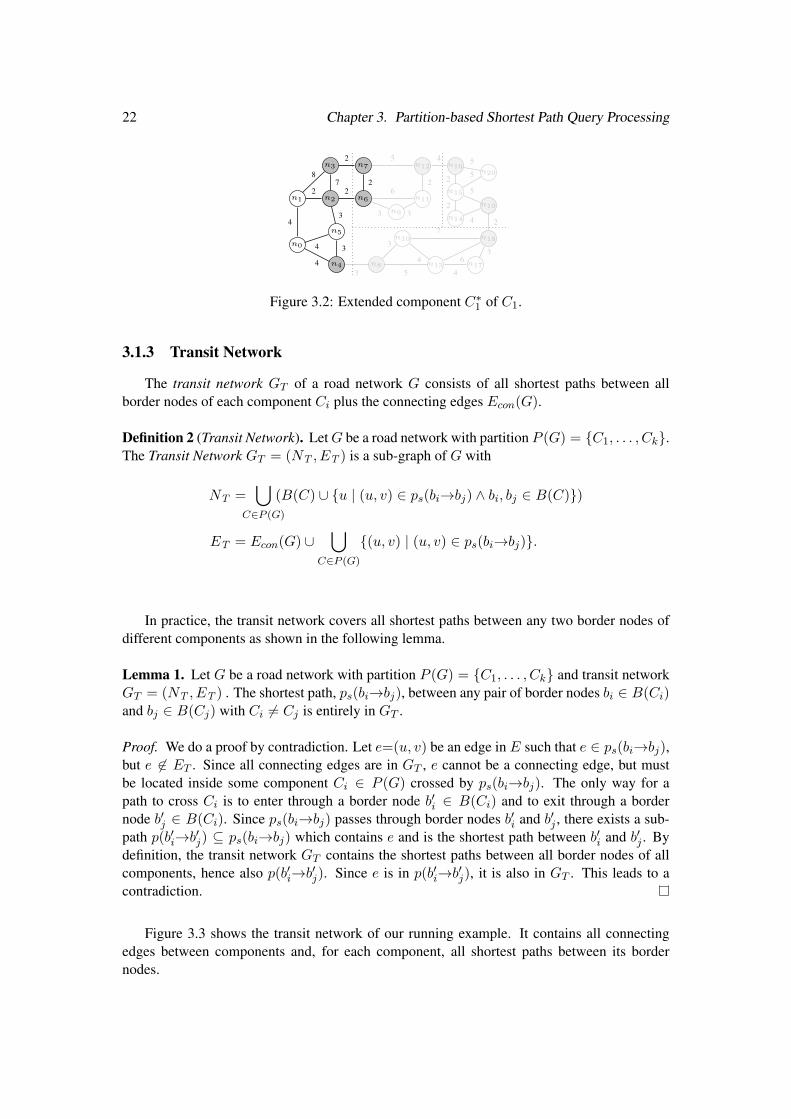
22 Chapter 3. Partition-based Shortest Path Query Processing
n0
n1 n2
n3
n4
n5
n6
n7
n8
n9
n10
n11
n12
n13
n14
n15
n16
n17
n18
n19
n20
4
4
4
2
87
3
3
2
2
2
3
3
6
5
3
5
3
4
7
2
4
4
6
2
4
25
5
5
3
2
Figure 3.2: Extended component C⇤1 of C1.
3.1.3 Transit Network
The transit network GT
of a road network G consists of all shortest paths between allborder nodes of each component C
i
plus the connecting edges Econ
(G).
Definition 2 (Transit Network). Let G be a road network with partition P (G) = {C1, . . . , Ck
}.The Transit Network G
T
= (NT
, ET
) is a sub-graph of G with
NT
=
[
C2P (G)
(B(C) [ {u | (u, v) 2 ps
(bi
!bj
) ^ bi
, bj
2 B(C)})
ET
= Econ
(G) [[
C2P (G)
{(u, v) | (u, v) 2 ps
(bi
!bj
)}.
In practice, the transit network covers all shortest paths between any two border nodes ofdifferent components as shown in the following lemma.
Lemma 1. Let G be a road network with partition P (G) = {C1, . . . , Ck
} and transit networkG
T
= (NT
, ET
) . The shortest path, ps
(bi
!bj
), between any pair of border nodes bi
2 B(Ci
)
and bj
2 B(Cj
) with Ci
6= Cj
is entirely in GT
.
Proof. We do a proof by contradiction. Let e=(u, v) be an edge in E such that e 2 ps
(bi
!bj
),but e 62 E
T
. Since all connecting edges are in GT
, e cannot be a connecting edge, but mustbe located inside some component C
i
2 P (G) crossed by ps
(bi
!bj
). The only way for apath to cross C
i
is to enter through a border node b0i
2 B(Ci
) and to exit through a bordernode b0
j
2 B(Ci
). Since ps
(bi
!bj
) passes through border nodes b0i
and b0j
, there exists a sub-path p(b0
i
!b0j
) ✓ ps
(bi
!bj
) which contains e and is the shortest path between b0i
and b0j
. Bydefinition, the transit network G
T
contains the shortest paths between all border nodes of allcomponents, hence also p(b0
i
!b0j
). Since e is in p(b0i
!b0j
), it is also in GT
. This leads to acontradiction.
Figure 3.3 shows the transit network of our running example. It contains all connectingedges between components and, for each component, all shortest paths between its bordernodes.

3.1. Preprocessing for ParDiSP 23
n0
n1 n2
n3
n4
n5
n6
n7
n8
n9
n10
n11
n12
n13
n14
n15
n16
n17
n18
n19
n20
3
2
2
3
3
2
5
3
7
4
25
24
4
4
2
87
3
6
3
5
4
2
4
63
2
4
5
5
Figure 3.3: Transit Network of the example road network.
3.1.4 Distance Tables and Component Distance Matrix
For each node in a component, we define an in-component distance table (IDT). The IDTof a node v 2 C
i
stores the distances from v to every border node of Ci
.
Definition 3 (In-component Distance Tables). Let G be a road network with partition P (G) =
{C1, . . . , Ck
}. The in-component distance table of a node v 2 Ci
is defined as
T (v) = {hbi
, d(v, bi
)i | bi
2 B(Ci
)}.
Figure 3.4 shows two IDTs. T (n0) stores the distances between n0 and the border nodesn2, n3 and n4 of component C1, whereas T (n20) stores the distances between n20 and theborder nodes n16 and n19 of component C3.
M
; M12 M14
M21 ; M23 M24
M31 M32 ; M34
M41 M42 M43 ;
T (n0)
n2 6n3 12n4 4
T (n20)
n16 5n19 10
M13
n2 n16 13n3 n16 11n4 n16 19n2 n19 20n3 n19 18n4 n19 15
Figure 3.4: IDTs for node n0 and n20 and CDM with entry (C1, C3).
Next, we compute the component distance matrix (CDM) of a partitioned road network.Given a partitioned road network G = (N,E), the CDM contains all the distances betweenborder nodes of any pair of components.
Definition 4 (Component Distance Matrix). Let G be a road network with partition P (G) =
{C1, . . . , Ck
}. The component distance matrix M is a k ⇥ k matrix, where each element isdefined as
Mij
=
8<
:{hu, v, d(u, v)i | u2B(C
i
) ^ v2B(Cj
)} i 6= j,
; i = j.
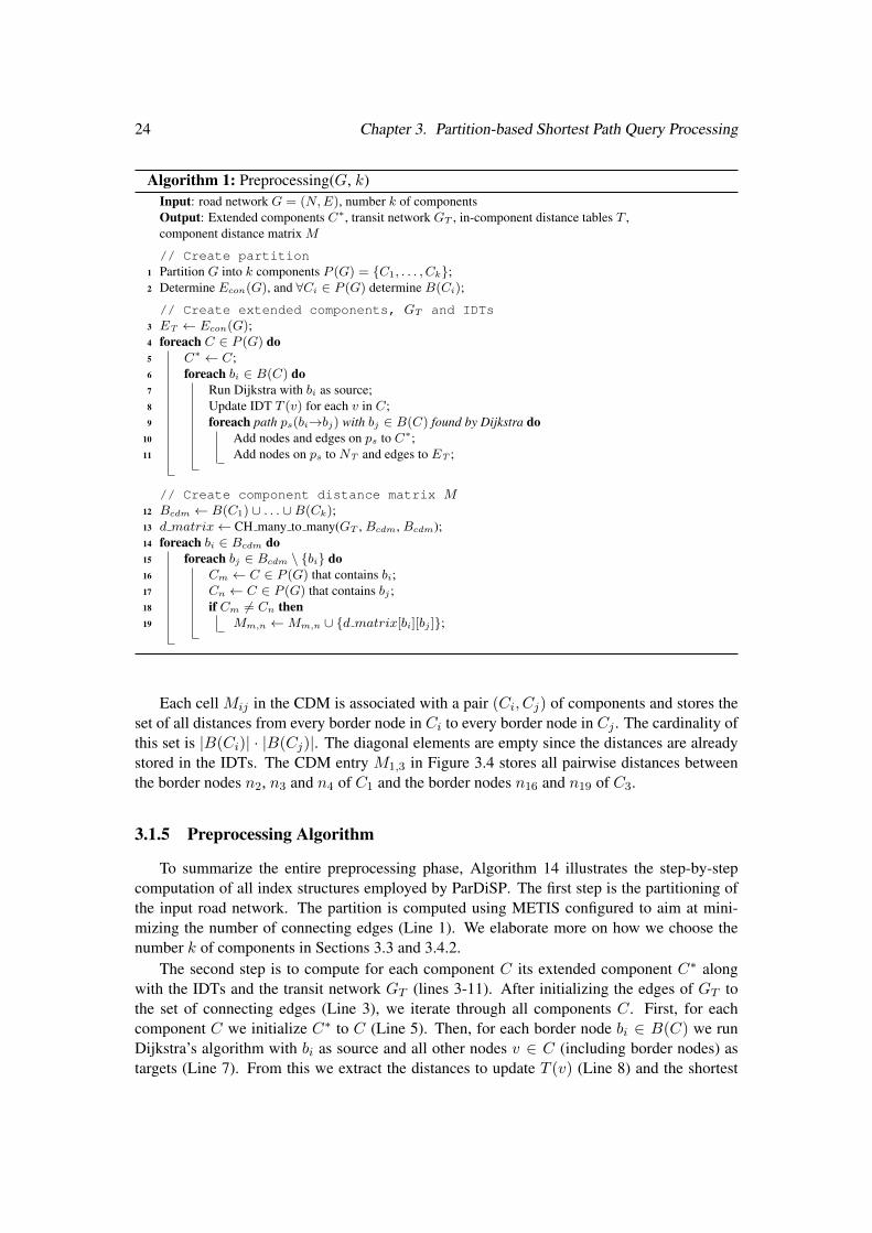
24 Chapter 3. Partition-based Shortest Path Query Processing
Algorithm 1: Preprocessing(G, k)Input: road network G = (N,E), number k of componentsOutput: Extended components C⇤, transit network G
T
, in-component distance tables T ,component distance matrix M
// Create partition1 Partition G into k components P (G) = {C1, . . . , Ck
};2 Determine E
con
(G), and 8Ci
2 P (G) determine B(Ci
);
// Create extended components, GT
and IDTs3 ET E
con
(G);4 foreach C 2 P (G) do5 C⇤ C;6 foreach b
i
2 B(C) do7 Run Dijkstra with b
i
as source;8 Update IDT T (v) for each v in C;9 foreach path p
s
(bi
!bj
) with bj
2 B(C) found by Dijkstra do10 Add nodes and edges on p
s
to C⇤;11 Add nodes on p
s
to NT and edges to ET ;
// Create component distance matrix M12 B
cdm
B(C1) [ . . . [B(Ck
);13 d matrix CH many to many(G
T
, Bcdm
, Bcdm
);14 foreach b
i
2 Bcdm
do15 foreach b
j
2 Bcdm
\ {bi
} do16 C
m
C 2 P (G) that contains bi
;17 C
n
C 2 P (G) that contains bj
;18 if C
m
6= Cn
then19 M
m,n
Mm,n
[ {d matrix[bi
][bj
]};
Each cell Mij
in the CDM is associated with a pair (Ci
, Cj
) of components and stores theset of all distances from every border node in C
i
to every border node in Cj
. The cardinality ofthis set is |B(C
i
)| · |B(Cj
)|. The diagonal elements are empty since the distances are alreadystored in the IDTs. The CDM entry M1,3 in Figure 3.4 stores all pairwise distances betweenthe border nodes n2, n3 and n4 of C1 and the border nodes n16 and n19 of C3.
3.1.5 Preprocessing Algorithm
To summarize the entire preprocessing phase, Algorithm 14 illustrates the step-by-stepcomputation of all index structures employed by ParDiSP. The first step is the partitioning ofthe input road network. The partition is computed using METIS configured to aim at mini-mizing the number of connecting edges (Line 1). We elaborate more on how we choose thenumber k of components in Sections 3.3 and 3.4.2.
The second step is to compute for each component C its extended component C⇤ alongwith the IDTs and the transit network G
T
(lines 3-11). After initializing the edges of GT
tothe set of connecting edges (Line 3), we iterate through all components C. First, for eachcomponent C we initialize C⇤ to C (Line 5). Then, for each border node b
i
2 B(C) we runDijkstra’s algorithm with b
i
as source and all other nodes v 2 C (including border nodes) astargets (Line 7). From this we extract the distances to update T (v) (Line 8) and the shortest

3.2. Query Processing with ParDiSP 25
paths to update C⇤ and GT
(lines 9-11).Finally, for the computation of the component distance matrix M we construct CH [36]
over the GT
and execute the many-to-many variant (Line 13). All border nodes of all compo-nents are used both as sources and as targets. The distance between every pair of border nodesis then added to the respective entry of M (lines 14-19).
3.2 Query Processing with ParDiSP
3.2.1 Processing Distance Queries
To compute distance queries from a source node s 2 Cs
to a target node t 2 Ct
, wedistinguish two cases:
1. s and t are in the same component
2. s and t are in different components.
First, if s and t are in the same component Ci
, we employ the ALT algorithm [38] overthe extended component C⇤
i
, which is essentially a bidirectional A⇤-search with landmarks.To compute a lower bound from any node n to the target node t, ALT hinges on the triangleinequality dist(n, t) � |dist(n, l) � dist(t, l)| for some landmark node l. We use the bordernodes of each component C
i
as landmarks, since the precomputed IDTs store all requireddistances to determine the lower bounds. Note that in case the A⇤-search expands a node thatis not in C (but in C⇤), the lower bound is set to 0. Such a strategy eagerly expands the nodesthat are in C⇤ but not in C.
Second, the distance between a source node s and a target node t that are located in differentcomponents C
s
and Ct
, respectively, is composed of three distances: the distance from s to aborder node b
s
of Cs
, the distance from a border node bt
of Ct
to t, and the distance from bs
tobt
, i.e.,
d(s, t) = min
b
s
2B(Cs
)b
t
2B(Ct
)
{d(s, bs
) + d(bs
, bt
) + d(bt
, t)}.
Since the three partial distances have already been precomputed and stored in the IDTs andin the CDM, the distance query amounts to joining three distance tables, regardless of how faraway the source and target nodes are. Figure 3.5 illustrates the three distance tables T (n0), M13
and T (N20) that are required to determine the distance from node n0 2 C1 to node n20 2 C20,along with the part of the road network that is accessed, i.e., C⇤
1 [GT
[ C⇤3 .
The algorithm to compute distance queries is shown in Algorithm 16. First, the componentsCs
and Ct
of the source node s and target node t, respectively, are determined (lines 1-2). IfCs
= Ct
, we execute ALT over the extended component C⇤s
(Line 4). Otherwise, if Cs
6= Ct
,we join the precomputed distance tables T (s), M
C
s
,C
t
, and T (t) (lines 6-15). The first loopjoins T (s) and the entry M
C
s
,C
t
of the component distance matrix, which yields the distancesbetween s and each border node of C
t
(lines 9-12). The second loop joins the intermediateresult in Ttmp with T (t) and determines the overall minimum distance, which is the distancefrom s to t (lines 13-15). Finally, the algorithm return the distance d from s to t in Line 16.

26 Chapter 3. Partition-based Shortest Path Query Processing
n0
n1 n2
n3
n4
n5
n6
n7
n8
n9
n10
n11
n12
n13
n14
n15
n16
n17
n18
n19
n20
4
4
4
2
87
32
3
5
5
4
52
2
2
3
3
7
45
2
3
6
5
3
4
2
4
63
2
C1
C2
C3
C4
T (n0)n2 6n3 12n4 4
M13
n2 n16 13n3 n16 11n4 n16 19n2 n19 20n3 n19 18n4 n19 15
T (n20)
n16 5n19 10
Figure 3.5: IDTs/CDM entry for a distance query from n0 to n20.
Algorithm 2: Distance Query(G, s, t)Input: road network G, source node s, target node tOutput: distance d(s, t)
1 Cs
C 2 P (G) that contains s;2 C
t
C 2 P (G) that contains t;
3 if Cs
= Ct
then4 d distance ALT(C⇤
s
, s, t);5 else6 T
tmp
empty array of size |T (t)|, initialized to1;7 d +1;8 k �1;9 for i = 0 to |M
Cs,Ct |� 1 do10 j i mod |T (s)|;11 if j = 0 then k k + 1;12 Ttmp [k] min(Ttmp [k], T (s)[j] + T2[i]);
13 for i = 0 to |T (t)|� 1 do14 d0 Ttmp [i] + T (t)[i];15 if d0 < d then d d0;
16 return d;
To achieve an efficient implementation of the joins, we keep for each component a sortedlist of border nodes. By doing so, the distance tables need to store only the distances (andnot the node ids) if they are sorted in the same order. Similarly, the entries of M store onlydistances. The entries are sorted first by the id of the target node and then by the id of thesource node. This implementation technique saves space by omitting the storage of node idsin the distance tables, and permits efficient joins of the tables since the indices of matchingelements can be computed directly.
Example 1. The execution of the algorithm is illustrated in Figure 3.6. The tables B(C1)
and B(C3) determine the sort order of the distance tables. The first entry of T (n0) stores thedistance from n0 to n2, whereas the first entry of T (n20) stores the distance from n16 to n20.The first loop joins T (n0) and M13 and produces the intermediate table Ttmp, which containsthe distances from n0 to the two border nodes n16 and n19 of C3. In the second loop, wesum one-to-one the elements of T
tmp
with the elements of T (n20) and keep the minimum, i.e.,19 + 5 = 24 is the distance between n0 and n20. This is possible since T
tmp
and T (t) areordered in the same way.
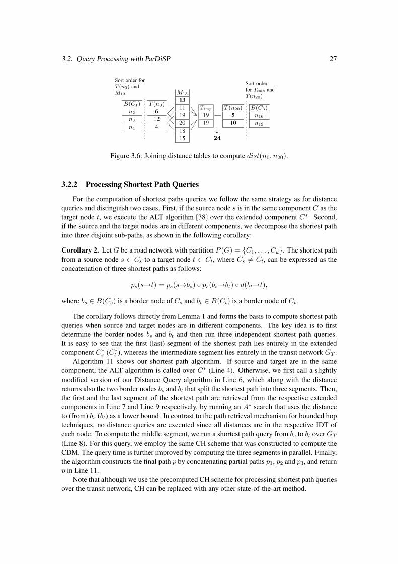
3.2. Query Processing with ParDiSP 27
B(C1)
n2
n3
n4
Sort order forT (n0) andM13
T (n0)
6124
M13
131119201815
Ttmp
1919
T (n20)
510
B(C3)
n16
n19
Sort orderfor Ttmp andT (n20)
24
Figure 3.6: Joining distance tables to compute dist(n0, n20).
3.2.2 Processing Shortest Path Queries
For the computation of shortest paths queries we follow the same strategy as for distancequeries and distinguish two cases. First, if the source node s is in the same component C as thetarget node t, we execute the ALT algorithm [38] over the extended component C⇤. Second,if the source and the target nodes are in different components, we decompose the shortest pathinto three disjoint sub-paths, as shown in the following corollary:
Corollary 2. Let G be a road network with partition P (G) = {C1, . . . , Ck
}. The shortest pathfrom a source node s 2 C
s
to a target node t 2 Ct
, where Cs
6= Ct
, can be expressed as theconcatenation of three shortest paths as follows:
ps
(s!t) = ps
(s!bs
) � ps
(bs
!bt
) � d(bt
!t),
where bs
2 B(Cs
) is a border node of Cs
and bt
2 B(Ct
) is a border node of Ct
.
The corollary follows directly from Lemma 1 and forms the basis to compute shortest pathqueries when source and target nodes are in different components. The key idea is to firstdetermine the border nodes b
s
and bt
and then run three independent shortest path queries.It is easy to see that the first (last) segment of the shortest path lies entirely in the extendedcomponent C⇤
s
(C⇤t
), whereas the intermediate segment lies entirely in the transit network GT
.Algorithm 11 shows our shortest path algorithm. If source and target are in the same
component, the ALT algorithm is called over C⇤ (Line 4). Otherwise, we first call a slightlymodified version of our Distance Query algorithm in Line 6, which along with the distancereturns also the two border nodes b
s
and bt
that split the shortest path into three segments. Then,the first and the last segment of the shortest path are retrieved from the respective extendedcomponents in Line 7 and Line 9 respectively, by running an A⇤ search that uses the distanceto (from) b
s
(bt
) as a lower bound. In contrast to the path retrieval mechanism for bounded hoptechniques, no distance queries are executed since all distances are in the respective IDT ofeach node. To compute the middle segment, we run a shortest path query from b
s
to bt
over GT
(Line 8). For this query, we employ the same CH scheme that was constructed to compute theCDM. The query time is further improved by computing the three segments in parallel. Finally,the algorithm constructs the final path p by concatenating partial paths p1, p2 and p3, and returnp in Line 11.
Note that although we use the precomputed CH scheme for processing shortest path queriesover the transit network, CH can be replaced with any other state-of-the-art method.
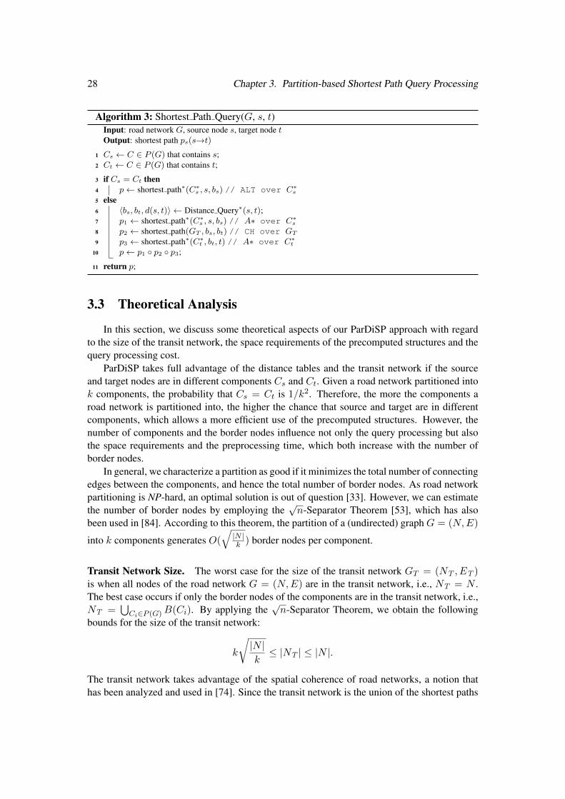
28 Chapter 3. Partition-based Shortest Path Query Processing
Algorithm 3: Shortest Path Query(G, s, t)Input: road network G, source node s, target node tOutput: shortest path p
s
(s!t)
1 Cs
C 2 P (G) that contains s;2 C
t
C 2 P (G) that contains t;
3 if Cs
= Ct
then4 p shortest path⇤
(C⇤s
, s, bs
) // ALT over C⇤s
5 else6 hb
s
, bt
, d(s, t)i Distance Query⇤(s, t);
7 p1 shortest path⇤(C⇤
s
, s, bs
) // A⇤ over C⇤s
8 p2 shortest path(GT
, bs
, bt
) // CH over GT
9 p3 shortest path⇤(C⇤
t
, bt
, t) // A⇤ over C⇤t
10 p p1 � p2 � p3;
11 return p;
3.3 Theoretical Analysis
In this section, we discuss some theoretical aspects of our ParDiSP approach with regardto the size of the transit network, the space requirements of the precomputed structures and thequery processing cost.
ParDiSP takes full advantage of the distance tables and the transit network if the sourceand target nodes are in different components C
s
and Ct
. Given a road network partitioned intok components, the probability that C
s
= Ct
is 1/k2. Therefore, the more the components aroad network is partitioned into, the higher the chance that source and target are in differentcomponents, which allows a more efficient use of the precomputed structures. However, thenumber of components and the border nodes influence not only the query processing but alsothe space requirements and the preprocessing time, which both increase with the number ofborder nodes.
In general, we characterize a partition as good if it minimizes the total number of connectingedges between the components, and hence the total number of border nodes. As road networkpartitioning is NP-hard, an optimal solution is out of question [33]. However, we can estimatethe number of border nodes by employing the
pn-Separator Theorem [53], which has also
been used in [84]. According to this theorem, the partition of a (undirected) graph G = (N,E)
into k components generates O(
q|N |k
) border nodes per component.
Transit Network Size. The worst case for the size of the transit network GT
= (NT
, ET
)
is when all nodes of the road network G = (N,E) are in the transit network, i.e., NT
= N .The best case occurs if only the border nodes of the components are in the transit network, i.e.,N
T
=
SC
i
2P (G)B(Ci
). By applying thepn-Separator Theorem, we obtain the following
bounds for the size of the transit network:
k
r|N |k |N
T
| |N |.
The transit network takes advantage of the spatial coherence of road networks, a notion thathas been analyzed and used in [74]. Since the transit network is the union of the shortest paths
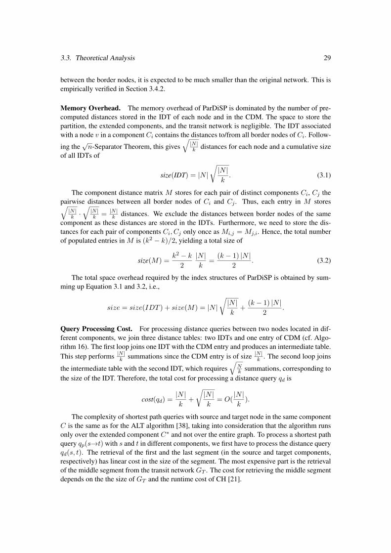
3.3. Theoretical Analysis 29
between the border nodes, it is expected to be much smaller than the original network. This isempirically verified in Section 3.4.2.
Memory Overhead. The memory overhead of ParDiSP is dominated by the number of pre-computed distances stored in the IDT of each node and in the CDM. The space to store thepartition, the extended components, and the transit network is negligible. The IDT associatedwith a node v in a component C
i
contains the distances to/from all border nodes of Ci
. Follow-
ing thepn-Separator Theorem, this gives
q|N |k
distances for each node and a cumulative sizeof all IDTs of
size(IDT) = |N |r
|N |k
. (3.1)
The component distance matrix M stores for each pair of distinct components Ci
, Cj
thepairwise distances between all border nodes of C
i
and Cj
. Thus, each entry in M storesq|N |k
·q
|N |k
=
|N |k
distances. We exclude the distances between border nodes of the samecomponent as these distances are stored in the IDTs. Furthermore, we need to store the dis-tances for each pair of components C
i
, Cj
only once as Mi,j
= Mj,i
. Hence, the total numberof populated entries in M is (k2 � k)/2, yielding a total size of
size(M) =
k2 � k
2
|N |k
=
(k � 1) |N |2
. (3.2)
The total space overhead required by the index structures of ParDiSP is obtained by sum-ming up Equation 3.1 and 3.2, i.e.,
size = size(IDT ) + size(M) = |N |r
|N |k
+
(k � 1) |N |2
.
Query Processing Cost. For processing distance queries between two nodes located in dif-ferent components, we join three distance tables: two IDTs and one entry of CDM (cf. Algo-rithm 16). The first loop joins one IDT with the CDM entry and produces an intermediate table.This step performs |N |
k
summations since the CDM entry is of size |N |k
. The second loop joins
the intermediate table with the second IDT, which requiresq
N
k
summations, corresponding tothe size of the IDT. Therefore, the total cost for processing a distance query q
d
is
cost(qd
) =
|N |k
+
r|N |k
= O(
|N |k
).
The complexity of shortest path queries with source and target node in the same componentC is the same as for the ALT algorithm [38], taking into consideration that the algorithm runsonly over the extended component C⇤ and not over the entire graph. To process a shortest pathquery q
p
(s!t) with s and t in different components, we first have to process the distance queryqd
(s, t). The retrieval of the first and the last segment (in the source and target components,respectively) has linear cost in the size of the segment. The most expensive part is the retrievalof the middle segment from the transit network G
T
. The cost for retrieving the middle segmentdepends on the the size of G
T
and the runtime cost of CH [21].

30 Chapter 3. Partition-based Shortest Path Query Processing
3.4 Experimental Evaluation
In this section, we describe the results of a detailed experimental evaluation of ParDiSPon real-world road networks. We analyze the runtime, the preprocessing cost and the memoryconsumption of ParDiSP in comparison to state-of-the-art methods for distance and shortestpath queries. Furthermore, we provide some additional measurements to back our claims re-garding the effect of road network partitioning to the preprocessing cost and the performanceof our ParDiSP approach.
3.4.1 Setup and Datasets
In our experimental evaluation we use four real-world public available datasets from the9th DIMACS Challenge1, each of which corresponds to a part of the road network in US. Thesedatasets are summarized in Table 3.1).
Table 3.1: Datasets.
Name Region # Nodes # EdgesNY New York City 264,346 733,846FL Florida 1,070,376 2,712,79CA California-Nevada 1,890,815 4,657,742E Eastern USA 3,598,623 8,778,114
We performed three sets of experiments in total. In the first set of experiments (Figures 3.7-3.11 and 3.13) we evaluate the performance of ParDiSP in terms of preprocessing cost, spaceoverhead and query processing time for different partitions of the same dataset varying thenumbers of components k from 128 to 1024.
In the second set of experiments (Figures 3.12, 3.14–3.16), we compare ParDiSP to threedifferent algorithms: Arterial Hierarchy (AH) [94], which has been shown to be the fastestapproach for shortest path queries [86]; Contraction Hierarchies (CH) [36], which we alsoemploy for the computation of the CDM; and Pruned Highway Labeling (PHL) [7], a state-of-the-art method for distance queries.
To determine the number of components k for ParDiSP for the second set of experiments,we use the insight we gained from the measurements of the first set. We observed that fordistance queries ParDiSP becomes faster as the number of components k is increasing while,for shortest path queries, ParDiSP shows the best performance for k = {256, 384, 512}. Sinceshortest path queries are more time consuming than distance queries we run our experimentsfor all datasets with k = 384. For the selected value of k, ParDiSP is adequately fast fordistance queries too.
Finally, in the third set of experiments (Figure 3.16), we analyze the query performancefor mixed query sets that contain both distance and shortest path queries. The ratio of distanceto shortest path queries in each query set varies between 20%/80%, 40%/60%, 60%/40%and 80%/20%. We compare ParDiSP with two combined approaches using state-of-the-artsolutions for each query type: PHL for distance queries and CH and AH, respectively, forshortest path queries, denoted as PHL-CH and PHL-AH.
1http://www.dis.uniroma1.it/challenge9/
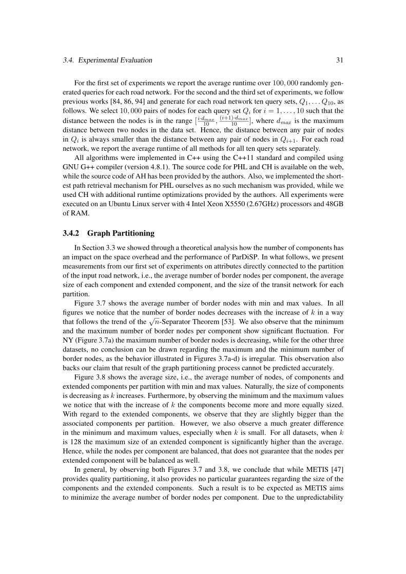
3.4. Experimental Evaluation 31
For the first set of experiments we report the average runtime over 100, 000 randomly gen-erated queries for each road network. For the second and the third set of experiments, we followprevious works [84, 86, 94] and generate for each road network ten query sets, Q1, . . . Q10, asfollows. We select 10, 000 pairs of nodes for each query set Q
i
for i = 1, . . . , 10 such that thedistance between the nodes is in the range [
i·dmax
10 , (i+1)·dmax
10 ], where dmax
is the maximumdistance between two nodes in the data set. Hence, the distance between any pair of nodesin Q
i
is always smaller than the distance between any pair of nodes in Qi+1. For each road
network, we report the average runtime of all methods for all ten query sets separately.All algorithms were implemented in C++ using the C++11 standard and compiled using
GNU G++ compiler (version 4.8.1). The source code for PHL and CH is available on the web,while the source code of AH has been provided by the authors. Also, we implemented the short-est path retrieval mechanism for PHL ourselves as no such mechanism was provided, while weused CH with additional runtime optimizations provided by the authors. All experiments wereexecuted on an Ubuntu Linux server with 4 Intel Xeon X5550 (2.67GHz) processors and 48GBof RAM.
3.4.2 Graph Partitioning
In Section 3.3 we showed through a theoretical analysis how the number of components hasan impact on the space overhead and the performance of ParDiSP. In what follows, we presentmeasurements from our first set of experiments on attributes directly connected to the partitionof the input road network, i.e., the average number of border nodes per component, the averagesize of each component and extended component, and the size of the transit network for eachpartition.
Figure 3.7 shows the average number of border nodes with min and max values. In allfigures we notice that the number of border nodes decreases with the increase of k in a waythat follows the trend of the
pn-Separator Theorem [53]. We also observe that the minimum
and the maximum number of border nodes per component show significant fluctuation. ForNY (Figure 3.7a) the maximum number of border nodes is decreasing, while for the other threedatasets, no conclusion can be drawn regarding the maximum and the minimum number ofborder nodes, as the behavior illustrated in Figures 3.7a-d) is irregular. This observation alsobacks our claim that result of the graph partitioning process cannot be predicted accurately.
Figure 3.8 shows the average size, i.e., the average number of nodes, of components andextended components per partition with min and max values. Naturally, the size of componentsis decreasing as k increases. Furthermore, by observing the minimum and the maximum valueswe notice that with the increase of k the components become more and more equally sized.With regard to the extended components, we observe that they are slightly bigger than theassociated components per partition. However, we also observe a much greater differencein the minimum and maximum values, especially when k is small. For all datasets, when kis 128 the maximum size of an extended component is significantly higher than the average.Hence, while the nodes per component are balanced, that does not guarantee that the nodes perextended component will be balanced as well.
In general, by observing both Figures 3.7 and 3.8, we conclude that while METIS [47]provides quality partitioning, it also provides no particular guarantees regarding the size of thecomponents and the extended components. Such a result is to be expected as METIS aimsto minimize the average number of border nodes per component. Due to the unpredictability

32 Chapter 3. Partition-based Shortest Path Query Processing
128 256 384 512 640 768 896 10240
30
60
90
120
150
k
Bor
dern
odes
/com
p.
(a) NY
128 256 384 512 640 768 896 10240
40
80
120
160
200
k
Bor
dern
odes
/com
p.
(b) FL
128 256 384 512 640 768 896 10240
60
120
180
240
300
k
Bor
dern
odes
/com
p.
(c) CA
128 256 384 512 640 768 896 10240
60
120
180
240
300
kB
orde
rnod
es/c
omp.
(d) E
Figure 3.7: Border nodes per partition.
128 256 384 512 640 768 896 10240
0.5
1
1.5
2
2.5
3
·103
k
#no
des
Component Extended Component
(a) NY
128 256 384 512 640 768 896 10240
2
4
6
8
10
12
·103
k
#no
des
(b) FL
128 256 384 512 640 768 896 10240
4
8
12
16
20
·103
k
#no
des
(c) CA
128 256 384 512 640 768 896 10240
10
20
30
40
·103
k
#no
des
(d) E
Figure 3.8: Component and extended component size per partition.
of graph partitioning, it is impossible to minimize the size of the extended components unlessboth the partition and the extended components are computed. On the other hand, minimizingthe average number of border nodes per component results in smaller IDTs and, hence, fasterprocessing of distance queries.
Figure 3.9 analyzes the number of nodes and edges of the resulting transit network. Thesize of the transit network increases with k, yet it is significantly smaller (approximately 2-5 times) than the the original road network. Hence, any query between border nodes can be

3.4. Experimental Evaluation 33
128 256 384 512 640 768 896 10240
0.1
0.2
0.3
0.4·106
k
#no
des
and
edge
s#Nodes #Edges
(a) NY
128 256 384 512 640 768 896 10240
0.2
0.4
0.6
0.8
1
·106
k
#no
des
and
edge
s
(b) FL
128 256 384 512 640 768 896 10240
0.3
0.6
0.9
1.2
1.5·106
k
#no
des
and
edge
s
(c) CA
128 256 384 512 640 768 896 10240
0.5
1
1.5
2
2.5
3
·106
k
#no
des
and
edge
s
(d) E
Figure 3.9: Transit network size per partition.
computed by accessing only a part of the road network which is only 1/2 to 1/5 the size of theoriginal. Furthermore, the space overhead of CH, which we build over the transit network, isexpected to decrease along with the number of components k.
For efficient query processing, apart from the size of the transit network, the density of thenetwork plays an important role too. The CH method that we use for queries over the transitnetwork works best for sparse networks. We observe though that the transit network is denserthan the original road network. The density of a road network is given by:
D(G) =
|E||D| · (|D|� 1)
.
For example, the density of the road network of NY is D(NY ) ' 10.5 ·10�6 while the densityof the the transit network varies from D(G
T
) ' 31 · 10�6 for k = 128 to D(GT
) ' 18 · 10�6
for k = 1024. In general, we observe that the density of the transit network decreases with theincrease of k. Hence, the more the components in a partition, the sparser the transit networkgets.
3.4.3 Preprocessing
Figure 3.10 analyzes the preprocessing time of ParDiSP varying the number k of compo-nents. We distinguish between the time for precomputing a) the extended components (C⇤)b) the IDTs and the transit network (G
T
+IDTs), and c) the CDM including the constructionof the CH scheme (CDM). In all figures, we observe that the time required to precompute theextended components decreases as k increases, whereas the time to precompute the CDM in-creases with k. Apparently, although more extended components need to be computed, sincethe size of the components and the number of border nodes decrease with k, each computa-tion of of an extended component requires much less time; thus the overall preprocessing time

34 Chapter 3. Partition-based Shortest Path Query Processing
128 256 384 512 640 768 896 10240
30
60
90
120
150
k
Run
time
(min
)C⇤ GT +IDTs CH+CDM
(a) NY
128 256 384 512 640 768 896 10240
150
300
450
600
k
Run
time
(min
)
(b) FL
128 256 384 512 640 768 896 10240
0.4
0.8
1.2
1.6·103
k
Run
time
(min
)
(c) CA
128 256 384 512 640 768 896 10240
1.5
3
4.5
6
·103
k
Run
time
(min
)
(d) E
Figure 3.10: Preprocessing time in ParDiSP.
drops. Next, we observe that the time required to compute the IDTs and the transit network issimilar for all values of k. On the contrary, the time required to compute the CDM increaseswith k, since the transit network becomes larger too. Also, the total number of border nodesincreases and, hence, there are more sources-targets in the many-to-many search. Finally, weobserve that for all datasets the preprocessing time shows a local minimum; for NY the prepro-cessing time is minimum for k = 512, for FL it is minimum for k = 384, for CA it is minimumfor k = 640 and for E it is minimum for k = 896.
Figure 3.11 shows the space overhead of ParDiSP varying the number k of components.We distinguish between the memory required to store a) the IDTs b) the CDM and c) theCH scheme over the transit network. The space required to store the extended componentsand the transit network is negligible. With an increasing number k of components, the spacerequired by the CDM increases, whereas the space for the IDTs decreases. The space requiredto store the CH scheme over the transit network slightly increases with k but it is negligible incomparison to the memory requirements for storing the IDTs and the CDM. Overall, with theexception of small values of k, the memory requirements are dominated by the CDM.
Figure 3.12 compares the preprocessing time and space overhead of ParDiSP (with k =
384) to AH, CH and PHL for all datasets. Figure 3.12a shows that CH outperforms ParDiSPand the other competitors in terms of preprocessing time on all datasets. For NY, PHL andParDiSP have similar preprocessing time while AH is the slowest. For FL and CA, PHL, AHand ParDiSP have similar preprocessing time while, for E, AH is the fastest method after CH,ParDiSP is slightly slower and PHL is the slowest method. Figure 3.12b analyzes the spaceoverhead. For NY all approaches have similar space requirements except for ParDiSP whichhas slightly more. For all the other datasets, CH is shown to consume the least space, followedby AH. PHL is the method which inflicts the highest space overhead by far. ParDiSP requiressignificantly less space than PHL, but more than CH and AH.
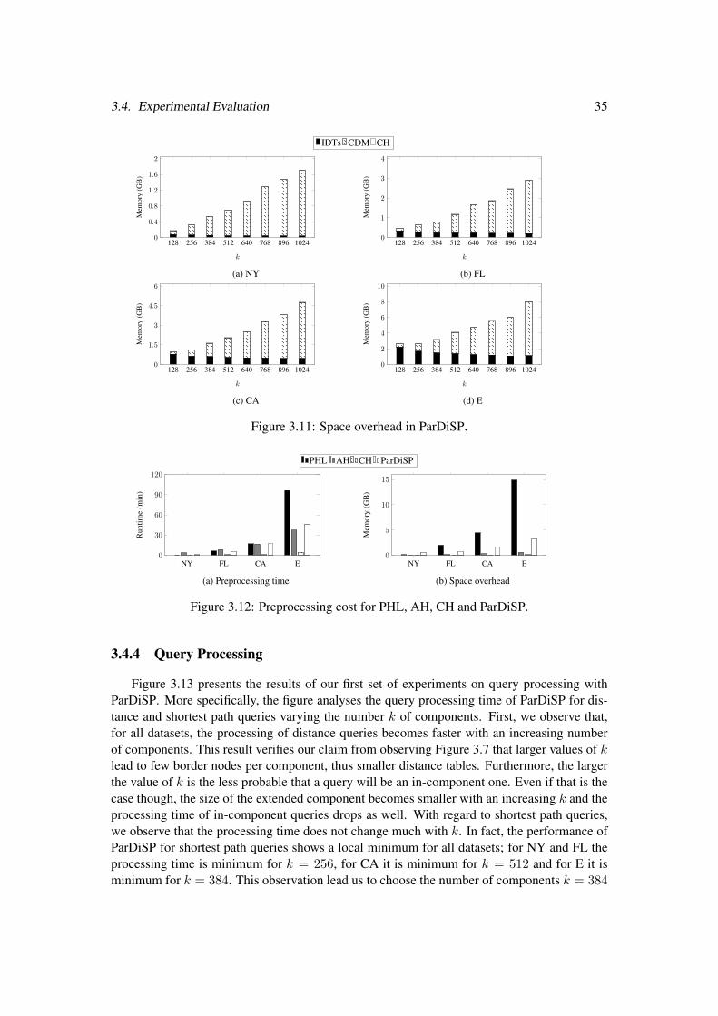
3.4. Experimental Evaluation 35
128 256 384 512 640 768 896 10240
0.4
0.8
1.2
1.6
2
k
Mem
ory
(GB
)IDTs CDM CH
(a) NY
128 256 384 512 640 768 896 10240
1
2
3
4
k
Mem
ory
(GB
)
(b) FL
128 256 384 512 640 768 896 10240
1.5
3
4.5
6
k
Mem
ory
(GB
)
(c) CA
128 256 384 512 640 768 896 10240
2
4
6
8
10
k
Mem
ory
(GB
)
(d) E
Figure 3.11: Space overhead in ParDiSP.
NY FL CA E0
30
60
90
120
Run
time
(min
)
PHL AH CH ParDiSP
(a) Preprocessing time
NY FL CA E0
5
10
15
Mem
ory
(GB
)
(b) Space overhead
Figure 3.12: Preprocessing cost for PHL, AH, CH and ParDiSP.
3.4.4 Query Processing
Figure 3.13 presents the results of our first set of experiments on query processing withParDiSP. More specifically, the figure analyses the query processing time of ParDiSP for dis-tance and shortest path queries varying the number k of components. First, we observe that,for all datasets, the processing of distance queries becomes faster with an increasing numberof components. This result verifies our claim from observing Figure 3.7 that larger values of klead to few border nodes per component, thus smaller distance tables. Furthermore, the largerthe value of k is the less probable that a query will be an in-component one. Even if that is thecase though, the size of the extended component becomes smaller with an increasing k and theprocessing time of in-component queries drops as well. With regard to shortest path queries,we observe that the processing time does not change much with k. In fact, the performance ofParDiSP for shortest path queries shows a local minimum for all datasets; for NY and FL theprocessing time is minimum for k = 256, for CA it is minimum for k = 512 and for E it isminimum for k = 384. This observation lead us to choose the number of components k = 384

36 Chapter 3. Partition-based Shortest Path Query Processing
128 256 384 512 640 768 896 10240
15
30
45
60
k
Run
time
(µs)
Distance Queries Shortest Path Queries
(a) NY
128 256 384 512 640 768 896 10240
30
60
90
120
150
k
Run
time
(µs)
(b) FL
128 256 384 512 640 768 896 10240
50
100
150
200
250
k
Run
time
(µs)
(c) CA
128 256 384 512 640 768 896 10240
100
200
300
400
500
k
Run
time
(µs)
(d) E
Figure 3.13: Cost of query processing in ParDiSP.
for our second set of experiments.Figures 3.14 and 3.15 report the results of our second set of experiments on the processing
time of distance and shortest path queries. In particular, Figure 3.14 compares the processingof distance queries with ParDiSP, AH, CH and PHL for all four datasets. In all datasets,the runtime of ParDiSP is constant, except for query set Q1, where the rate of in-componentqueries is comparably high. Clearly, processing in-component queries with ParDiSP is moreexpensive than processing cross-component queries. While PHL is the fastest solution for allfour datasets, ParDiSP is very close to this state-of-the-art solution. CH is approximately oneorder of magnitude slower than both ParDiSP and PHL and alt least two times slower thanAH, especially for query sets Q5 to Q10 Finally, we observe that, in all road networks, theperformance of AH deteriorates in the beginning, but improves significantly after Q4, i.e.,while the distance between query points increases. It appears that AH is better at processingqueries where the query points are far apart. However, even for Q10 where AH shows the bestperformance, it is still slower than our ParDiSP approach.
Figure 3.15 compares the processing of shortest path queries with ParDiSP, AH, CH andPHL for all four datasets. First, for the NY dataset we observe in Figure 3.15a that, althoughPHL is the fastest method for distance queries, it is extremely inefficient for shortest pathqueries. The reason for this poor performance is the large number of distance queries that needto be processed for retrieving the shortest path. Naturally, the performance of PHL deteriorateseven more for query sets where the query points are distant. For presentation purposes, we omitPHL in Figures 3.15b–3.15d.
With regard to the other algorithms, we observe that, for NY, AH and ParDiSP have similarperformance (with AH being sightly faster) while CH is clearly the slowest approach amongthe three. ParDiSP is the fastest approach in FL, CA and E, outperforming both CH and AHfor all query sets, with the exception of Q1 for the CA road network. Since the source and thetarget points of queries in Q1 are very close, the number of in-component queries that ParDiSP
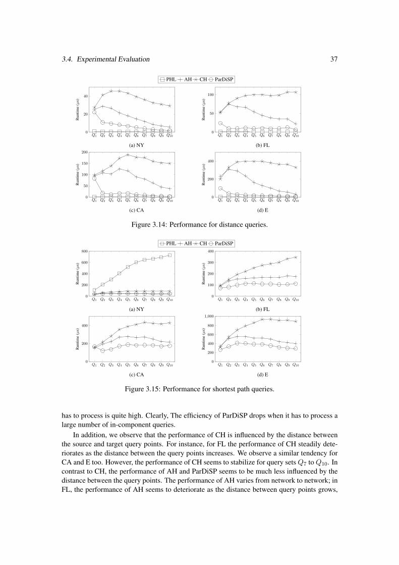
3.4. Experimental Evaluation 37
Q1 Q2 Q3 Q4 Q5 Q6 Q7 Q8 Q9 Q100
20
40
Run
time
(µs)
PHL AH CH ParDiSP
(a) NY
Q1 Q2 Q3 Q4 Q5 Q6 Q7 Q8 Q9 Q100
50
100
Run
time
(µs)
(b) FL
Q1 Q2 Q3 Q4 Q5 Q6 Q7 Q8 Q9 Q100
50
100
150
200
Run
time
(µs)
(c) CA
Q1 Q2 Q3 Q4 Q5 Q6 Q7 Q8 Q9 Q100
200
400
Run
time
(µs)
(d) E
Figure 3.14: Performance for distance queries.
Q1 Q2 Q3 Q4 Q5 Q6 Q7 Q8 Q9 Q100
200
400
600
800
Run
time
(µs)
PHL AH CH ParDiSP
(a) NY
Q1 Q2 Q3 Q4 Q5 Q6 Q7 Q8 Q9 Q100
100
200
300
400
Run
time
(µs)
(b) FL
Q1 Q2 Q3 Q4 Q5 Q6 Q7 Q8 Q9 Q100
200
400
Run
time
(µs)
(c) CA
Q1 Q2 Q3 Q4 Q5 Q6 Q7 Q8 Q9 Q100
200
400
600
800
1,000
Run
time
(µs)
(d) E
Figure 3.15: Performance for shortest path queries.
has to process is quite high. Clearly, The efficiency of ParDiSP drops when it has to process alarge number of in-component queries.
In addition, we observe that the performance of CH is influenced by the distance betweenthe source and target query points. For instance, for FL the performance of CH steadily dete-riorates as the distance between the query points increases. We observe a similar tendency forCA and E too. However, the performance of CH seems to stabilize for query sets Q7 to Q10. Incontrast to CH, the performance of AH and ParDiSP seems to be much less influenced by thedistance between the query points. The performance of AH varies from network to network; inFL, the performance of AH seems to deteriorate as the distance between query points grows,

38 Chapter 3. Partition-based Shortest Path Query Processing
Q1 Q2 Q3 Q4 Q5 Q6 Q7 Q8 Q9 Q100
20
40
60
80
Run
time
(µs)
PHL-AH PHL-CH ParDiSP
NY
Q1 Q2 Q3 Q4 Q5 Q6 Q7 Q8 Q9 Q100
100
200
300
Run
time
(µs)
FL
Q1 Q2 Q3 Q4 Q5 Q6 Q7 Q8 Q9 Q100
100
200
300
400
Run
time
(µs)
CA
Q1 Q2 Q3 Q4 Q5 Q6 Q7 Q8 Q9 Q100
200
400
600
800
Run
time
(µs)
E
(a) |Qd
| = 20%, |Qp
| = 80%
Q1 Q2 Q3 Q4 Q5 Q6 Q7 Q8 Q9 Q100
20
40
60
Run
time
(µs)
NY
Q1 Q2 Q3 Q4 Q5 Q6 Q7 Q8 Q9 Q100
50
100
150
200
250
Run
time
(µs)
FL
Q1 Q2 Q3 Q4 Q5 Q6 Q7 Q8 Q9 Q100
100
200
300
Run
time
(µs)
CA
Q1 Q2 Q3 Q4 Q5 Q6 Q7 Q8 Q9 Q100
200
400
600
Run
time
(µs)
E
(b) |Qd
| = 40%, |Qp
| = 60%
Q1 Q2 Q3 Q4 Q5 Q6 Q7 Q8 Q9 Q100
10
20
30
40
Run
time
(µs)
NY
Q1 Q2 Q3 Q4 Q5 Q6 Q7 Q8 Q9 Q100
50
100
150
Run
time
(µs)
FL
Q1 Q2 Q3 Q4 Q5 Q6 Q7 Q8 Q9 Q100
50
100
150
200
Run
time
(µs)
CA
Q1 Q2 Q3 Q4 Q5 Q6 Q7 Q8 Q9 Q100
100
200
300
400
Run
time
(µs)
E
(c) |Qd
| = 60%, |Qp
| = 40%
Q1 Q2 Q3 Q4 Q5 Q6 Q7 Q8 Q9 Q100
10
20
30
40
Run
time
(µs)
NY
Q1 Q2 Q3 Q4 Q5 Q6 Q7 Q8 Q9 Q100
20
40
60
80
Run
time
(µs)
FL
Q1 Q2 Q3 Q4 Q5 Q6 Q7 Q8 Q9 Q100
20
40
60
80
100
120
Run
time
(µs)
CA
Q1 Q2 Q3 Q4 Q5 Q6 Q7 Q8 Q9 Q100
50
100
150
200
Run
time
(µs)
E
(d) |Qd
| = 80%, |Qp
| = 20%
Figure 3.16: Performance for mixed query sets.
in CA, the performance does not deteriorate and appears to be most efficient for query sets Q2
and Q3, while in E, the performance deteriorates from Q1 to Q3 but then, from Q3 to Q10 itimproves steadily. The performance of ParDiSP is similar for all query sets.
Finally, Figure 3.16 shows the results of our third set of experiments with mixed querysets. For NY, PHL-AH is the fastest approach outperforming ParDiSP. For Q1 of CA, theperformance of ParDiSP displays a similar behavior as in our previous experiments, meaningthat the number of in-component queries is quite high. However, in all settings apart from NYand Q1 of CA, ParDiSP clearly outperforms both PHL-CH and PHL-AH. We also observe that

3.5. Summary 39
the gap between ParDiSP and the two competitors gets smaller with the increase of distancequeries in the query load. When more than 95% of the queries are distance queries, the threeapproaches have comparable performance for FL, CA and E. Finally, we observe that PHL-AHoutperforms PHL-CH for all settings. Such a result is expected as both methods use PHL fordistance queries, while AH is faster than CH in shortest path queries.
3.5 Summary
We presented ParDiSP, a framework for the efficient processing of both distance and short-est path queries on road networks. Given an input road network partitioned into components,ParDiSP precomputes a set of index structures which are utilized to optimize query processing.ParDiSP answers distance and shortest path queries by running the ALT algorithm if sourceand target are in the same component, using the precomputed distances to the border nodesto compute lower bounds. Otherwise, for distance queries, ParDiSP combines distances fromthree precomputed tables, whereas shortest path queries are decomposed into the retrieval ofthree sub-paths, which can be executed in parallel. Our experimental evaluation has shownthat ParDiSP outperforms the state-of-the-art for shortest path queries, while being comparableto the state-of-the-art for distance queries. For mixed query sets with distance and shortestpath queries, ParDiSP is, in most cases, more efficient even than a combination of the beststate-of-the-art approaches for the two query types, while incurring less space overhead.


CHAPTER 4
k-Shortest Paths with Limited Overlap
In this chapter, we introduce a novel approach to tackle the problem of computing alter-native paths on road networks. Our focus is to recommend a set of k paths (including theshortest path) such that every path in the result set is sufficiently dissimilar to all the otherpaths in the result set based on a user-specified similarity threshold and, at the same time, asshort as possible. We formalize this form of alternative routing as the k-Shortest Paths withLimited Overlap (k-SPwLO) problem. Furthermore, we propose three algorithms for evaluat-ing k-SPwLO queries. The baseline algorithm BSL computes first a (necessarily large) set ofcandidate paths and applies similarity filtering in a second step. OnePass traverses the networkonce and expands only those paths that qualify the similarity constraint. Finally, MultiPassextends and improves OnePass by employing an additional pruning criterion and computesk-SPwLO queries by traversing the network k�1 times.
41
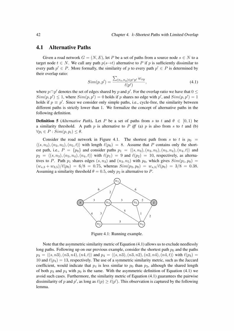
42 Chapter 4. k-Shortest Paths with Limited Overlap
4.1 Alternative Paths
Given a road network G = (N,E), let P be a set of paths from a source node s 2 N to atarget node t 2 N . We call any path p(s!t) alternative to P if p is sufficiently dissimilar toevery path p0 2 P . More formally, the similarity of p to every path p0 2 P is determined bytheir overlap ratio:
Sim(p, p0) =
P(n
x
,n
y
)2p\p0 wxy
`(p0), (4.1)
where p\ p0 denotes the set of edges shared by p and p0. For the overlap ratio we have that 0 Sim(p, p0) 1, where Sim(p, p0) = 0 holds if p shares no edge with p0, and Sim(p, p0) = 1
holds if p ⌘ p0. Since we consider only simple paths, i.e., cycle-free, the similarity betweendifferent paths is strictly lower than 1. We formalize the concept of alternative paths in thefollowing definition.
Definition 5 (Alternative Path). Let P be a set of paths from s to t and ✓ 2 [0, 1) bea similarity threshold. A path p is alternative to P iff (a) p is also from s to t and (b)8p
i
2 P : Sim(p, pi
) ✓.
Consider the road network in Figure 4.1. The shortest path from s to t is p0 =
h(s, n3), (n3, n5), (n5, t)i with length `(p0) = 8. Assume that P contains only the short-est path, i.e., P = {p0} and consider paths p1 = h(s, n3), (n3, n5), (n5, n4), (n4, t)i andp2 = h(s, n3), (n3, n4), (n4, t)i with `(p1) = 9 and `(p2) = 10, respectively, as alterna-tives to P . Path p1 shares edges (s, n3) and (n3, n5) with p0, which gives Sim(p1, p0) =
(ws,3 + w3,5)/`(p0) = 6/8 = 0.75, whereas Sim(p2, p0) = w
s,3/`(p0) = 3/8 = 0.38.Assuming a similarity threshold ✓ = 0.5, only p2 is alternative to P .
s
n1
n2
n3
n4
n5 t
6
4
3
26
3
5
5
3
12
2
Figure 4.1: Running example.
Note that the asymmetric similarity metric of Equation (4.1) allows us to exclude needlesslylong paths. Following up on our previous example, consider the shortest path p0 and the pathsp3 = h(s, n3), (n3, n4), (n4, t)i and p4 = h(s, n3), (n3, n2), (n2, n4), (n4, t)i with `(p3) =
10 and `(p4) = 13, respectively. The use of a symmetric similarity metric, such as the Jaccardcoefficient, would indicate that p4 is less similar to p0 than p3, although the shared lengthof both p3 and p4 with p0 is the same. With the asymmetric definition of Equation (4.1) weavoid such cases. Furthermore, the similarity metric of Equation (4.1) guarantees the pairwisedissimilarity of p and p0, as long as `(p) � `(p0). This observation is captured by the followinglemma.

4.2. k-Shortest Paths with Limited Overlap 43
Lemma 3. Given two paths p, p0 where `(p) � `(p0), and a similarity threshold ✓, iffSim(p, p0) < ✓ then also Sim(p0, p) < ✓.
Proof. Following Equation (4.1) for the similarity between p and p0 and given that `(p) � `(p0),we have:
P(n
x
,n
y
)2p\p0 wxy
`(p)
P(n
x
,n
y
)2p\p0 wxy
`(p0)) Sim(p0, p) Sim(p, p0).
Therefore, iff Sim(p, p0) < ✓ then also Sim(p0, p) < ✓.
4.2 k-Shortest Paths with Limited Overlap
We now introduce the problem of k-Shortest Paths with Limited Overlap (k-SPwLO).Given a source node s and a target node t, the goal is to recommend a set of k paths froms to t, sorted by length in increasing order such that (a) the shortest path p0(s!t) is alwaysincluded, (b) every path is dissimilar to its predecessors with respect to a similarity threshold✓, and (c) all k paths are as short as possible. Intuitively, this task can also be seen as pro-gressively recommending k paths to the user starting from the shortest path p0. Every pathpi
recommended next is alternative to the set of paths already recommended and as short aspossible. We formalize the k-SPwLO problem in the following definition.
Definition 6 (k-SPwLO). Given a road network G = (N,E), a source node s 2 N ,a target node t 2 N , a requested number of paths k and a similarity threshold ✓. Ak�SPwLO(s, t, ✓, k) query returns a set PLO = {p0, . . . , p
k�1} of k paths from s to t, forwhich the following holds:
• p0 is the shortest path from s to t,
• 8pi
, pj
2 PLO with i 6= j: Sim(pi
, pj
) ✓, and
• 8p /2 PLO one of the following two conditions holds:
– `(p) � `(pi
) holds 8pi
2 PLO– 9p
i
2 PLO with `(pi
) `(p) and Sim(p, pi
) > ✓.
The first bullet of Definition 6 guarantees that the shortest path p0(s!t) is always in theresult set PLO. The second bullet assures that the recommended paths in PLO are sufficientlydissimilar to each other. Finally, the third bullet guarantees that PLO contains the shortestamong all paths qualifying the previous constraints. More specifically, every path p that is notpart of the k-SPwLO, is either longer than all the paths in the set (Condition 1), or there is ashorter path p
i
in the set which causes p to violate the similarity constraint (Condition 2).A naıve approach for computing k-SPwLO queries is to iterate over all paths from the
source node s to the target node t and compute their pairwise similarity. However, such asolution is impractical; for real-world road networks, it is impossible to offline precompute andstore all paths connecting any pair of nodes as the enumeration of all possible paths is a #P -complete problem [83]. In what follows, we present three algorithms for processing k-SPwLOqueries (Sections 4.3-4.5) which examine paths in increasing length order and built the resultset progressively.
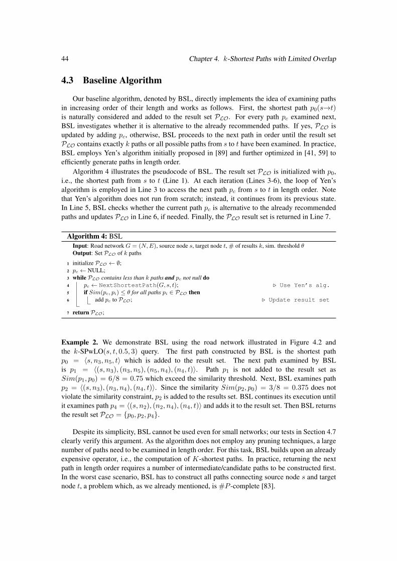
44 Chapter 4. k-Shortest Paths with Limited Overlap
4.3 Baseline Algorithm
Our baseline algorithm, denoted by BSL, directly implements the idea of examining pathsin increasing order of their length and works as follows. First, the shortest path p0(s!t)is naturally considered and added to the result set PLO. For every path p
c
examined next,BSL investigates whether it is alternative to the already recommended paths. If yes, PLO isupdated by adding p
c
, otherwise, BSL proceeds to the next path in order until the result setPLO contains exactly k paths or all possible paths from s to t have been examined. In practice,BSL employs Yen’s algorithm initially proposed in [89] and further optimized in [41, 59] toefficiently generate paths in length order.
Algorithm 4 illustrates the pseudocode of BSL. The result set PLO is initialized with p0,i.e., the shortest path from s to t (Line 1). At each iteration (Lines 3-6), the loop of Yen’salgorithm is employed in Line 3 to access the next path p
c
from s to t in length order. Notethat Yen’s algorithm does not run from scratch; instead, it continues from its previous state.In Line 5, BSL checks whether the current path p
c
is alternative to the already recommendedpaths and updates PLO in Line 6, if needed. Finally, the PLO result set is returned in Line 7.
Algorithm 4: BSLInput: Road network G = (N,E), source node s, target node t, # of results k, sim. threshold ✓Output: Set PLO of k paths
1 initialize PLO ;;2 p
c
NULL;3 while PLO contains less than k paths and p
c
not null do4 p
c
NextShortestPath(G, s, t); . Use Yen’s alg.5 if Sim(p
c
, pi
) ✓ for all paths pi
2 PLO then6 add p
c
to PLO; . Update result set
7 return PLO;
Example 2. We demonstrate BSL using the road network illustrated in Figure 4.2 andthe k-SPwLO(s, t, 0.5, 3) query. The first path constructed by BSL is the shortest pathp0 = hs, n3, n5, ti which is added to the result set. The next path examined by BSLis p1 = h(s, n3), (n3, n5), (n5, n4), (n4, t)i. Path p1 is not added to the result set asSim(p1, p0) = 6/8 = 0.75 which exceed the similarity threshold. Next, BSL examines pathp2 = h(s, n3), (n3, n4), (n4, t)i. Since the similarity Sim(p2, p0) = 3/8 = 0.375 does notviolate the similarity constraint, p2 is added to the results set. BSL continues its execution untilit examines path p4 = h(s, n2), (n2, n4), (n4, t)i and adds it to the result set. Then BSL returnsthe result set PLO = {p0, p2, p4}.
Despite its simplicity, BSL cannot be used even for small networks; our tests in Section 4.7clearly verify this argument. As the algorithm does not employ any pruning techniques, a largenumber of paths need to be examined in length order. For this task, BSL builds upon an alreadyexpensive operator, i.e., the computation of K-shortest paths. In practice, returning the nextpath in length order requires a number of intermediate/candidate paths to be constructed first.In the worst case scenario, BSL has to construct all paths connecting source node s and targetnode t, a problem which, as we already mentioned, is #P -complete [83].

4.4. OnePass Algorithm 45
s
n1
n2
n3
n4
n5 t
6
4
3
26
3
5
5
3
12
2
shortest path (p0) 1st alt. (p2) 2nd alt. (p4)
Pall
p0 h(s, n3), (n3, n5), (n5, t)i 8p1 h(s, n3), (n3, n5), (n5, n4), (n4, t)i 9p2 h(s, n3), (n3, n4), (n4, t)i 10p3 h(s, n3), (n3, n4), (n4, n5), (n5, t)i 11p4 h(s, n3), (n3, n1), (n1, t)i 11p5 h(s, n2), (n2, n4), (n4, t)i 11p6 h(s, n2), (n2, n4), (n4, n5), (n5, t)i 12p7 h(s, n2), (n2, n3), (n3, n5), (n5, t)i 12p8 h(s, n1), (n1, t)i 12p9 h(s, n3), (n3, n2), (n2, n4), (n4, t)i 13
(. . . )
Figure 4.2: Computation of k-SPwLO (s,t,0.5,3) query with BSL.
4.4 OnePass Algorithm
OnePass, our second algorithm, traverses the road network starting from source node s ex-panding only paths that satisfy the similarity constraint ✓. Hence, the number of paths examinedby OnePass for the computation of a k-SPwLO query is significantly lower than the number ofpaths examined by BSL. In what follows, we formally introduce this pruning criterion and wepresent the OnePass algorithm which employs it.
4.4.1 Pruning Overlaping Sub-paths
Let p(s!n) be a path connecting source node s to some node n, and pi
(s!t) 2 PLO bean already recommended path. Assume that p is extended to reach target t, resulting in pathp0(s!t). As p0 contains all edges shared by p and p
i
, its similarity with pi
is at least equal to thesimilarity of p with p
i
, i.e., Sim(p0, pi
) � Sim(p, pi
). Hence, given a similarity threshold ✓, ifthere exists p
i
2 PLO such that Sim(p, pi
) � ✓, path p can be safely discarded; no extensionof p can possibly be an alternative path. This pruning criterion is formally captured by thefollowing lemma:
Lemma 4. Let PLO be the set of already recommended paths. If p is an alternative path toPLO with respect to a similarity threshold ✓ then Sim(p0, p
i
) ✓ holds for every subpath p0 ofp and any p
i
2 PLO.
Proof. Let p be an alternative path to PLO, i.e., 8pi
2 PLO : Sim(p, pi
) ✓. Consider asubpath p0 of p and denote by E
p�p
0 the set of edges contained in p but not in p0. FollowingEquation (4.1), for the overlap ratio of p and p0 and 8p
i
2 PLO we have:
Sim(p, pi
) = Sim(p0, pi
) +
P(n
x
,n
y
)2Ep�p
0 wxy
`(pi
)
from which we get
Sim(p0, pi
) Sim(p, pi
)) Sim(p0, pi
) ✓.
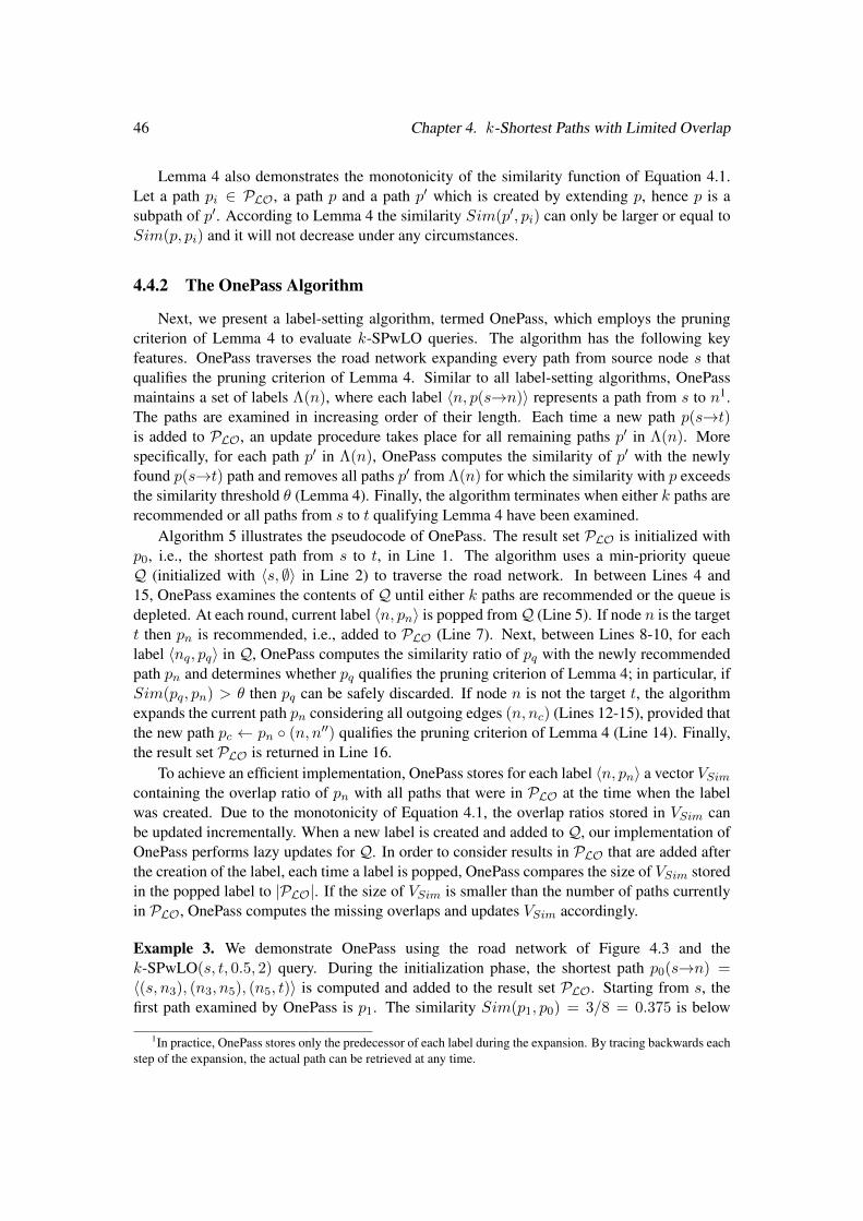
46 Chapter 4. k-Shortest Paths with Limited Overlap
Lemma 4 also demonstrates the monotonicity of the similarity function of Equation 4.1.Let a path p
i
2 PLO, a path p and a path p0 which is created by extending p, hence p is asubpath of p0. According to Lemma 4 the similarity Sim(p0, p
i
) can only be larger or equal toSim(p, p
i
) and it will not decrease under any circumstances.
4.4.2 The OnePass Algorithm
Next, we present a label-setting algorithm, termed OnePass, which employs the pruningcriterion of Lemma 4 to evaluate k-SPwLO queries. The algorithm has the following keyfeatures. OnePass traverses the road network expanding every path from source node s thatqualifies the pruning criterion of Lemma 4. Similar to all label-setting algorithms, OnePassmaintains a set of labels ⇤(n), where each label hn, p(s!n)i represents a path from s to n1.The paths are examined in increasing order of their length. Each time a new path p(s!t)is added to PLO, an update procedure takes place for all remaining paths p0 in ⇤(n). Morespecifically, for each path p0 in ⇤(n), OnePass computes the similarity of p0 with the newlyfound p(s!t) path and removes all paths p0 from ⇤(n) for which the similarity with p exceedsthe similarity threshold ✓ (Lemma 4). Finally, the algorithm terminates when either k paths arerecommended or all paths from s to t qualifying Lemma 4 have been examined.
Algorithm 5 illustrates the pseudocode of OnePass. The result set PLO is initialized withp0, i.e., the shortest path from s to t, in Line 1. The algorithm uses a min-priority queueQ (initialized with hs, ;i in Line 2) to traverse the road network. In between Lines 4 and15, OnePass examines the contents of Q until either k paths are recommended or the queue isdepleted. At each round, current label hn, p
n
i is popped from Q (Line 5). If node n is the targett then p
n
is recommended, i.e., added to PLO (Line 7). Next, between Lines 8-10, for eachlabel hn
q
, pq
i in Q, OnePass computes the similarity ratio of pq
with the newly recommendedpath p
n
and determines whether pq
qualifies the pruning criterion of Lemma 4; in particular, ifSim(p
q
, pn
) > ✓ then pq
can be safely discarded. If node n is not the target t, the algorithmexpands the current path p
n
considering all outgoing edges (n, nc
) (Lines 12-15), provided thatthe new path p
c
pn
� (n, n00) qualifies the pruning criterion of Lemma 4 (Line 14). Finally,
the result set PLO is returned in Line 16.To achieve an efficient implementation, OnePass stores for each label hn, p
n
i a vector VSim
containing the overlap ratio of pn
with all paths that were in PLO at the time when the labelwas created. Due to the monotonicity of Equation 4.1, the overlap ratios stored in V
Sim
canbe updated incrementally. When a new label is created and added to Q, our implementation ofOnePass performs lazy updates for Q. In order to consider results in PLO that are added afterthe creation of the label, each time a label is popped, OnePass compares the size of V
Sim
storedin the popped label to |PLO|. If the size of V
Sim
is smaller than the number of paths currentlyin PLO, OnePass computes the missing overlaps and updates V
Sim
accordingly.
Example 3. We demonstrate OnePass using the road network of Figure 4.3 and thek-SPwLO(s, t, 0.5, 2) query. During the initialization phase, the shortest path p0(s!n) =
h(s, n3), (n3, n5), (n5, t)i is computed and added to the result set PLO. Starting from s, thefirst path examined by OnePass is p1. The similarity Sim(p1, p0) = 3/8 = 0.375 is below
1In practice, OnePass stores only the predecessor of each label during the expansion. By tracing backwards eachstep of the expansion, the actual path can be retrieved at any time.
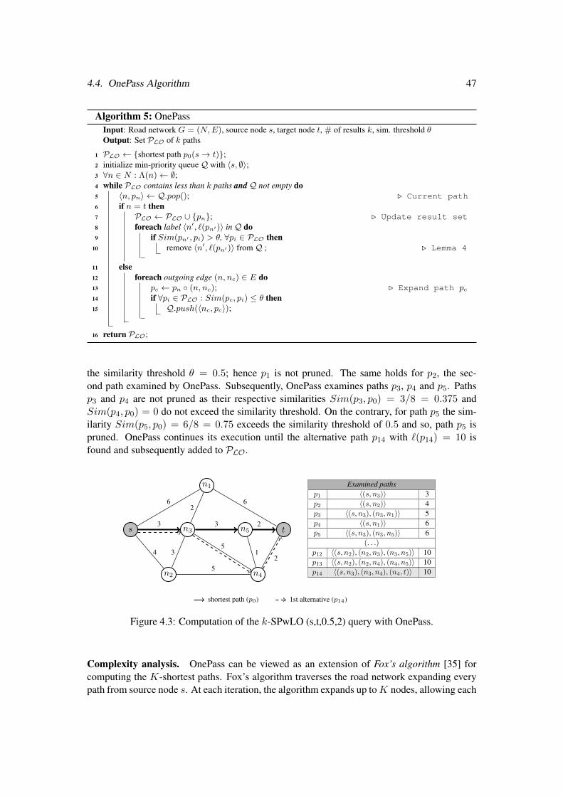
4.4. OnePass Algorithm 47
Algorithm 5: OnePassInput: Road network G = (N,E), source node s, target node t, # of results k, sim. threshold ✓Output: Set PLO of k paths
1 PLO {shortest path p0(s! t)};2 initialize min-priority queue Q with hs, ;i;3 8n 2 N : ⇤(n) ;;4 while PLO contains less than k paths and Q not empty do5 hn, p
n
i Q.pop(); . Current path6 if n = t then7 PLO PLO [ {p
n
}; . Update result set8 foreach label hn0, `(p
n
0)i in Q do
9 if Sim(pn
0 , pi
) > ✓, 8pi
2 PLO then10 remove hn0, `(p
n
0)i from Q ; . Lemma 4
11 else12 foreach outgoing edge (n, n
c
) 2 E do13 p
c
pn
� (n, nc
); . Expand path pc
14 if 8pi
2 PLO : Sim(pc
, pi
) ✓ then15 Q.push(hn
c
, pc
i);
16 return PLO;
the similarity threshold ✓ = 0.5; hence p1 is not pruned. The same holds for p2, the sec-ond path examined by OnePass. Subsequently, OnePass examines paths p3, p4 and p5. Pathsp3 and p4 are not pruned as their respective similarities Sim(p3, p0) = 3/8 = 0.375 andSim(p4, p0) = 0 do not exceed the similarity threshold. On the contrary, for path p5 the sim-ilarity Sim(p5, p0) = 6/8 = 0.75 exceeds the similarity threshold of 0.5 and so, path p5 ispruned. OnePass continues its execution until the alternative path p14 with `(p14) = 10 isfound and subsequently added to PLO.
s
n1
n2
n3
n4
n5 t
6
4
3
26
3
5
5
3
12
2
shortest path (p0) 1st alternative (p14)
Examined pathsp1 h(s, n3)i 3p2 h(s, n2)i 4p3 h(s, n3), (n3, n1)i 5p4 h(s, n1)i 6p5 h(s, n3), (n3, n5)i 6
(. . .)p12 h(s, n2), (n2, n3), (n3, n5)i 10p13 h(s, n2), (n2, n4), (n4, n5)i 10p14 h(s, n3), (n3, n4), (n4, t)i 10
Figure 4.3: Computation of the k-SPwLO (s,t,0.5,2) query with OnePass.
Complexity analysis. OnePass can be viewed as an extension of Fox’s algorithm [35] forcomputing the K-shortest paths. Fox’s algorithm traverses the road network expanding everypath from source node s. At each iteration, the algorithm expands up to K nodes, allowing each

48 Chapter 4. k-Shortest Paths with Limited Overlap
node to be expanded up to K times, and terminates when the target node has been expandedK times. The time complexity of Fox’s algorithm is O(|E|+K · |N | · log |N |). In contrast toFox’s algorithm, OnePass allows each node to be visited an unlimited number of times. Eachnode can be visited by OnePass as many times as the number of paths from s to t. OnePassterminates when either k paths are recommended or all paths from s to t qualifying Lemma 4are examined. Hence, the complexity of OnePass is O(|E| + K · |N | · log |N |), where K isthe number of shortest paths that have to be computed in order to cover the k results of thek-SPwLO query.
4.5 MultiPass Algorithm
Despite employing the pruning criterion of Lemma 4, OnePass still has to expand andexamine a large portion of all possible p(s!t) paths. In this section, we propose a novel label-setting algorithm, termed MultiPass, to enhance the computation of k-SPwLO. The algorithmemploys an additional powerful pruning criterion which significantly reduces the search spaceby avoiding expanding non-promising paths.
4.5.1 Pruning Non-Promising Paths
Let p0(s!t) be the shortest path from a source node s to a target node t as illustrated inFigure 4.4. In addition, let p
i
(s!n) and pj
(s!n) be two distinct paths from source s to anode n of the shortest path p0 such that `(p
i
) < `(pj
). Assuming that both pi
, pj
are extendedto reach target t following the same path p(n!t), any extension of p
i
will be shorter than therespective extension of p
j
. Furthermore, let Sim(pi
, p0) Sim(pj
, p0), i.e., the similarityof p
i
with p0 is equal or lower than the similarity of pj
with p0. Due to the monotonicity ofthe similarity function (Equation (4.1)), any extension of p
i
to n will have the same or lesssimilarity with p0 compared to the respective extension of p
j
. In other words, for any extensionof p
j
there will always be a shorter extension of pi
with less or equal similarity with p0; thus,pj
can be pruned.
s n tp0
pi
pj
Figure 4.4: Pruning paths with Lemma 5.
The same idea can be utilized to prune the search space when computing the short-est alternative path to a set of paths P . Consider again p
i
,pj
with `(pi
) < `(pj
) andSim(p
i
, p0) Sim(pj
, p0). Path pj
is pruned if for every path p 2 P the similarity Sim(pi
, p)is lower or equal to Sim(p
j
, p). This pruning criterion is formally captured by the followinglemma:
Lemma 5. Let P be a set of paths from a source node s to a target node t, and pi
, pj
be twopaths from s to some node n. If `(p
j
) > `(pi
) and 8p 2 P : Sim(pi
, p) Sim(pj
, p) holdthen path p
j
cannot be part of the shortest alternative path to P and we write pi
�P
pj
.

4.5. MultiPass Algorithm 49
Proof. We prove the lemma by contradiction. Assume that an extension p0j
=
h(s, ⇤), . . . , (⇤, n), . . . , (⇤, t)i of pj
(s!n) to target t is the shortest alternative path to P . Then,we show that an extension p0
i
= h(s, ⇤), . . . , (⇤, n), . . . , (⇤, t)i of pi
(s!n) to target t is also analternative path and it will be examined and recommended before p0
j
.According to the definition of an alternative path, Sim(p0
j
, p) ✓ holds 8p 2 P , andfollowing Lemma 4 Sim(p
j
, p) ✓ also holds 8p 2 P . Furthermore, due to the 8p 2 PLO :
Sim(pi
, p) Sim(pj
, p) assumption of Lemma 5, we get that Sim(pi
, p) ✓ holds 8p 2 P .As extension paths p0
i
and p0j
share the same sequence of edges connecting n to target t, wededuce that (a) Sim(p0
i
, p) ✓ holds 8p 2 P , i.e., p0i
is alternative to P and (b) `(p0i
) < `(p0j
)
which means that p0i
will be examined before p0j
.
The pruning criterion of Lemma 5 can be utilized to compute the shortest alternative pathto a set of paths as follows. Let P be the set of paths for which we want to compute theshortest alternative path, and P
n
the set of paths from s to some node n created during theexpansion of all paths from s. If P
n
contains a path p0(s!n) such that (a) p0 is longer thanany path p
n
2 Pn
\ {p0}, and (b) for every path p 2 P the similarity Sim(p0, p) is higher thanSim(p
n
, p) for all paths pn
2 Pn
\ {p0}, then p0 can be pruned. Note that the addition of a pathin P
n
may render condition (b) not applicable for another path already contained in Pn
. Toensure that set P
n
contains only paths for which both (a) and (b) hold, every time a new path isadded to P
n
, we have to check whether condition (b) still holds for all paths in the set.The aforementioned pruning criterion cannot be employed directly for the computation of
k-SPwLO queries. Consider again the example in Figure 4.4. Let p0 be the only path in the setof currently recommended alternative paths P . If during the search for the alternative path p1to P , p
j
is pruned because pi
�P
pj
holds, pj
cannot be part of the shortest alternative to P .However, there is no guarantee that p
j
will not be part of the shortest alternative to both p0 andp1. In particular, if p
i
is part of p1, then, during the search for the next alternative path, i.e.,the alternative path to P = {p0, p1}, p
i
may be pruned much earlier by Lemma 4. Hence, wehave to compute k-SPwLO queries in an iterative way. Each time a new alternative is addedto the k-SPwLO result set, we have to re-start the search for the next alternative path from thebeginning.
4.5.2 The MultiPass Algorithm
Next, we present MultiPass, a label-setting algorithm which employs both pruning criteriaof Lemma 4 and Lemma 5 to enhance the computation of k-SPwLO queries. The algorithmhas the following key features. For each node n of the road network, MultiPass maintains aset of labels ⇤(n). Each label represents a path from s to n and is of the form hn, p(s!n)i2.MultiPass traverses the road network k-1 times. At each iteration, the algorithm examines pathsfrom s in increasing order of their length and expands every path p(s!n) from s to a node nfor which the following holds: (a) its similarity with any already computed result does notexceed the input threshold ✓ (Lemma 4) and (b) its extension can possibly lead to the shortestalternative path during the current iteration (Lemma 5). Every time a new path p
n
(s!n) thatqualifies conditions (a) and (b) is found, a label hn, p
n
i is added to ⇤(n) and MultiPass removesall paths from ⇤(n) which do not qualify condition (b) anymore. As soon as a path to targett is found, MultiPass terminates current round, discards all stored labels, and re-traverses the
2Similar to OnePass, MultiPass stores only the predecessor of each label during the expansion.

50 Chapter 4. k-Shortest Paths with Limited Overlap
Algorithm 6: MultiPassInput: Road network G = (N,E), source node s, target node t, # of results k, similarity threshold ✓Output: Set PLO of k paths
1 PLO {shortest path p0(s!t)};2 while |PLO| < k and last round updated PLO do3 initialize min-priority queue Q with hs, ;i;4 8n 2 N : ⇤(n) ;;5 while Q not empty do6 hn, p
n
i Q.pop(); . Current path7 if n = t then8 PLO PLO [ {p
n
}; . Update result set9 break;
10 else11 foreach outgoing edge (n, n
c
) 2 E do12 p
c
pn
� (n, nc
); . Expand path pc
13 if 9pi
2 PLO : Sim(pc
, pi
)�✓ then14 continue; . Pruned by Lemma 415 else if 9hn
c
, p0c
i 2 ⇤(nc
) : p0c
�PLO pc
then16 continue; . Pruned by Lemma 517 else18 remove from Q and ⇤(n
c
) all hnc
, p0c
i : pc
�PLO p0c
; . Lemma 519 Q.push(hn
c
, pc
i);20 ⇤(n
c
) ⇤(nc
) [ {hnc
, pc
i};
21 return PLO;
network from source s. The algorithm terminates after k paths are added to result set PLO orthe last round failed to find an alternative path. In the latter case, a complete set of k-SPwLOwith respect to given ✓ and k values cannot be computed.
Algorithm 6 illustrates the pseudocode of MultiPass. The result set PLO is initialized withthe shortest path p0(s!t) (Line 1). The algorithm employs a min priority queue Q to traversethe road network. Before each traversal round, Q is initialized to hs, ;i (Line 3) and eachnode n is associated with a (initially empty) set of labels ⇤(n) (Line 4). At each round inbetween Lines 5 and 20, MultiPass pops label hn, p
n
i for current path pn
in Line 6. If n is thetarget t, then p
n
is added to PLO and the round terminates (Lines 7–9). Otherwise, MultiPassexpands the current path p
n
considering all outgoing edges (n, nc
) (Lines 10-16). Each newpath p
c
pn
�(n, nc
) (Line 12) is evaluated against the pruning criteria of Lemma 4 (Lines 13-14) and Lemma 5 (Lines 15-16). If p
c
qualifies both pruning criteria, MultiPass removes fromQ and ⇤(n
c
) every label representing a path p0n
such that pc
�PLO p0n
(Line 19). Finally, thenew label is added to Q (Line 19) and ⇤(n
c
) (Line 20) and the next label is popped from Q.The loop terminates after k paths are added to PLO or the last round failed to find an alternativepath. Finally, the PLO result set is returned in Line 21.
To achieve an efficient implementation, similar to OnePass, MultiPass also stores for eachlabel hn, p
n
i a vector VSim
containing the overlap ratio of pn
with all paths that were in PLOat the time when the label was created. The overlap ratios stored in V
Sim
are updated incre-mentally. When a new label is added to Q, MultiPass performs lazy updates for Q. Finally,each time a label is popped, MultiPass compares the size of V
Sim
stored in the popped label to
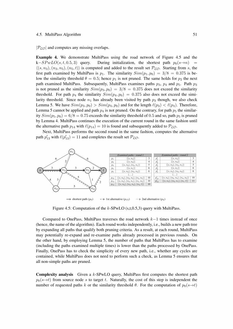
4.5. MultiPass Algorithm 51
|PLO| and computes any missing overlaps.
Example 4. We demonstrate MultiPass using the road network of Figure 4.5 and thek�SPwLO(s, t, 0.5, 3) query. During initialization, the shortest path p0(s!n) =
h(s, n3), (n3, n5), (n5, t)i is computed and added to the result set PLO. Starting from s, thefirst path examined by MultiPass is p1. The similarity Sim(p1, p0) = 3/8 = 0.375 is be-low the similarity threshold ✓ = 0.5; hence p1 is not pruned. The same holds for p2 the nextpath examined MultiPass. Subsequently, MultiPass examines paths p3, p4 and p5. Path p3is not pruned as the similarity Sim(p3, p0) = 3/8 = 0.375 does not exceed the similaritythreshold. For path p4 the similarity Sim(p4, p0) = 0.375 also does not exceed the simi-larity threshold. Since node n1 has already been visited by path p3 though, we also checkLemma 5. We have Sim(p3, p0) > Sim(p4, p0) and for the length `(p3) < `(p4). Therefore,Lemma 5 cannot be applied and path p4 is not pruned. On the contrary, for path p5 the similar-ity Sim(p5, p0) = 6/8 = 0.75 exceeds the similarity threshold of 0.5 and so, path p5 is prunedby Lemma 4. MultiPass continues the execution of the current round in the same fashion untilthe alternative path p14 with `(p14) = 10 is found and subsequently added to PLO.
Next, MultiPass performs the second round in the same fashion, computes the alternativepath p013 with `(p013) = 11 and completes the result set PLO.
s
n1
n2
n3
n4
n5 t
6
4
3
26
3
5
5
3
12
2
shortest path (p0) 1st alternative (p15) 2nd alternative (p4)
Examined paths - round 1p1 h(s, n3)i 3p2 h(s, n2)i 4p3 h(s, n3), (n3, n1)i 5p4 h(s, n1)i 6p5 h(s, n3), (n3, n2)i 6
(. . .)p12 h(s, n2), (n2, n3), (n3, n5)i 10p13 h(s, n2), (n2, n4), (n4, n5)i 10p14 h(s, n3), (n3, n4), (n4, t)i 10
Examined paths - round 2p01 h(s, n3)i 3p02 h(s, n2)i 4p03 h(s, n3), (n3, n1)i 5p04 h(s, n1)i 6p05 h(s, n3), (n3, n2)i 6
(. . .)p012 h(s, n2), (n2, n4), (n4, n5)i 10p013 h(s, n3), (n3, n1), (n1, t)i 11
Figure 4.5: Computation of the k-SPwLO (s,t,0.5,3) query with MultiPass.
Compared to OnePass, MultiPass traverses the road network k�1 times instead of once(hence, the name of the algorithm). Each round works independently, i.e., builds a new path treeby expanding all paths that qualify both pruning criteria. As a result, at each round, MultiPassmay potentially re-expand and re-examine paths already processed in previous rounds. Onthe other hand, by employing Lemma 5, the number of paths that MultiPass has to examine(including the paths examined multiple times) is lower than the paths processed by OnePass.Finally, OnePass has to check the simplicity of every new path, i.e., whether any cycles arecontained, while MultiPass does not need to perform such a check, as Lemma 5 ensures thatall non-simple paths are pruned.
Complexity analysis Given a k-SPwLO query, MultiPass first computes the shortest pathp0(s!t) from source node s to target t. Naturally, the cost of this step is independent thenumber of requested paths k or the similarity threshold ✓. For the computation of p0(s!t)

52 Chapter 4. k-Shortest Paths with Limited Overlap
any shortest path algorithm can be employed, e.g., Dijkstra’s algorithm [32] which requiresO(|E|+ |N | · log |N |).
To find each subsequent alternative path, all paths from source s that qualify the pruning cri-terion of Lemma 4 are expanded. However, as the value of the similarity threshold ✓ approaches1, the number of paths pruned by Lemma 4 significantly drops. In such a case, the result setis the K-Shortest paths. Furthermore in practice, there exists no formula for estimating thenumber of paths pruned by the pruning criterion of Lemma 5. Hence, each round of MultiPassbecomes equivalent to Fox’s algorithm [35] with a complexity O(|E|+K ·|N |·log |N |), whereK is the number of the shortest paths that have to be computed to cover the k-SPwLO result.Since k�1 rounds are required to compute a k-SPwLO query, the total runtime complexity ofMultiPass is O(k(|E| +K · |N | · log |N |)) where K >> k. As we explained in Section 4.2,the number of paths that have to be computed in order to cover the k-SPwLO set is very high;in extreme cases MultiPass may have to construct all paths from s to t.
Finally, note that the time complexity of MultiPass is worse than the time complexity ofOnePass. However, we show in our experimental evaluation that MultiPass is much fasterthan OnePass. The reason for this inconsistency is that although by employing the pruningcriterion of Lemma 5 MultiPass examines much less paths than OnePass, there can be noformal guarantees for the number of paths that are pruned. Although MultiPass has worsetheoretical time complexity though, in practice it is much more efficient than OnePass.
4.6 Optimization
To further improve the performance of OnePass and MultiPass we employ a lower bound,d(n, t), for the network distance d(n, t) of every node n to the target t. By employing such alower bound, both algorithm traverse the network in an A⇤-like fashion and direct the searchtowards the target, which avoids visiting nodes that are far away. In order to derive tight d(n, t)lower bounds, we first reverse the edges of the road network and then run Dijkstra’s algorithmfrom target t to every node n of the network [71]. In practice, at the beginning of the executionof both OnePass and MultiPass, instead of simply computing the shortest path from s to t, wecompute the shortest path tree from target t to each node n in the road network.
4.7 Experimental Evaluation
4.7.1 Experimental Setup
To demonstrate the efficiency of our algorithms, we measure the performance of BSL,OnePass and MultiPass using real road networks. To assess the runtime performance, we mea-sure the average response time over 1,000 random queries (i.e., pairs of nodes), varying thenumber k of requested paths, the similarity threshold ✓ and the distance between the querypoints in a similar fashion as in Section 3.4.1. In the first two experiments, we vary one ofthe two parameters and fix the other to its default value: 3 for k and 0.5 for ✓; in the thirdexperiment we fix both k and ✓ to their default values. All algorithms were implemented inC++ using the C++11 standard and compiled using GNU G++ compiler (version 4.8.1). Allexperiments were executed on an Ubuntu Linux server with 4 Intel Xeon X5550 (2.67GHz)processors and 48GB of RAM.

4.7. Experimental Evaluation 53
Due to the high execution time of BSL and OnePass, our experiments involve only the roadnetworks for the city of Oldenburg (6,105 nodes and 14,058 edges) and the city of San Joaquin(18,263 nodes and 47,594 edges). We also consider a timeout of 120 seconds. Each query thatfails to execute within the predefined timeout is considered failed.
4.7.2 Performance
The continuous lines in Figures 4.6-4.8 show the time for the queries for which all al-gorithms finished their execution in less than 120 seconds (successful queries), whereas thedashed lines show the time for all 1,000 queries including those which did not finish within120 seconds (timed-out/failed queries). In both figures we observe in that BSL is clearly im-practical. In fact, without the timeout, the response time of BSL would have been several ordersof magnitude higher than MultiPass (even with timeout MultiPass is from one to almost 4 or-ders of magnitude faster). Naturally, this is due to the large number of paths examined by BSLin length order, i.e., the paths returned by Yen’s algorithm. Hence, for presentation purposes,we report the results of BSL only for Oldenburg.
2 3 4 5
0
20
40
60
80
100
k
Res
pons
etim
e(s
ec)
BSL (suc) OnePass (suc.) MultiPass (suc.) BSL (all) OnePass (all) MultiPass (all)
(a) Oldenburg (✓=50%)
2 3 4 5
0
20
40
60
80
100
k
Res
pons
etim
e(s
ec)
(b) San Joaquin (✓=50%)
Figure 4.6: Performance comparison varying requested paths k (✓=50%).
Next, we observe that the performance of both OnePass and MultiPass deteriorates as thenumber k of requested paths increases. For all values of k though, MultiPass is clearly fasterthan OnePass. In most cases, MultiPass is at least two times faster. Another interesting obser-vation is that the performance curve of OnePass is almost linear, that is each iteration requiresapproximately the same time, e.g., for Oldenburg (Figure 4.6a) the algorithm needs similar timeto find the third and the fourth alternative path. On the other hand, MultiPass needs more timefor each subsequent result. This behavior can be explained by the fact that MultiPass restartsand re-expands paths.
With regard to parameter ✓, we observe in Figure 4.7 that in all cases, MultiPass is fasterthan OnePass. Especially for the lowest values of ✓, i.e., 0,1 and 0.3, MultiPass outperformsOnePass by at least an order of magnitude. The performance of OnePass is close to MultiPassonly for ✓=0.9, where the computed alternative paths can be very similar. Furthermore, thefact that the performance of OnePass and MultiPass deteriorates as ✓ increases, indicates thatthe pruning power of Lemma 4 deteriorates. However at the same time, we observe that forsmall values of ✓ the performance of MultiPass improves. This result indicates that for smallvalues of ✓ the pruning power of Lemma 5 increases.
Finally, Figure 4.8 compares the response time of all algorithms varying the distance be-tween query points. For all algorithms we observe that their performance deteriorates as the

54 Chapter 4. k-Shortest Paths with Limited Overlap
0.1 0.3 0.5 0.7 0.90
30
60
90
120
✓
Res
pons
etim
e(s
ec)
BSL (suc.) OnePass (suc.) MultiPass (suc.) BSL (all) OnePass (all) MultiPass (all)
(a) Oldenburg (k=3)
0.1 0.3 0.5 0.7 0.90
20
40
60
80
100
✓
Res
pons
etim
e(s
ec)
(b) San Joaquin (k=3)
Figure 4.7: Performance comparison varying similarity threshold ✓ (k=3).
distance between query points increases. Once again it is clear that BSL is the slowest algo-rithm, OnePass is faster than BSL, while MultiPass is clearly the fastest algorithm as it beatsboth BSL and OnePass. However, in Figure 4.8b we also observe that, even though MultiPassis the fastest algorithm, for Q5, where the distance between query points is the highest, Multi-Pass requires more than ten seconds to compute the k-SPwLO; thus, for larger road networks,MultiPass may not be very practical.
Q1 Q2 Q3 Q4 Q50
30
60
90
120
✓
Num
bero
flab
els
BSL (suc) OnePass (suc.) MultiPass (suc.) BSL (all) OnePass (all) MultiPass (all)
(a) Oldenburg
Q1 Q2 Q3 Q4 Q50
30
60
90
120
✓
Num
bero
flab
els
(b) San Joaquin
Figure 4.8: Performance comparison varying distance between s and t nodes (k=3, ✓ = 50%).
4.7.3 Memory Consumption
To provide a better insight on the performance of MultiPass and OnePass, we report inFigures 4.9 and 4.10 the number of labels each algorithm needs to examine before returningthe k-SPwLO result. We observe that, in all scenarios, MultiPass examines significantly fewerpaths than OnePass (even though we count the total number of paths from all rounds of Multi-Pass, hence some paths may be counted more than once).
With respect to the similarity threshold ✓, the result verifies our claim in Section 4.7.2regarding the pruning power of Lemmas 4 and reflm:prune2. As ✓ increases, the pruning powerof Lemma 4 deteriorates, and both OnePass and MultiPass construct more paths. However atthe same time, the next result can be determined earlier and, hence, the total runtime drops.In addition, as ✓ decreases, the pruning power of Lemma 5 increases, and more partial pathscan be pruned. This explains the behavior of MultiPass, where the number of examined pathsinitially increases, but after ✓=0.5 it goes down.

4.8. Summary 55
2 3 4 5
10
3
10
4
10
5
10
6
10
7
10
8
k
Num
bero
flab
els
OnePass (suc.) MultiPass (suc.) OnePass (all) MultiPass (all)
(a) Oldenburg (✓=50%)
2 3 4 5
10
3
10
4
10
5
10
6
10
7
10
8
10
9
k
Num
bero
flab
els
(b) San Joaquin (✓=50%)
Figure 4.9: Comparison of examined paths varying requested paths k (✓=5�%).
0.1 0.3 0.5 0.7 0.9
10
3
10
4
10
5
10
6
10
7
10
8
✓
Num
bero
flab
els
OnePass (suc.) MultiPass (suc.) OnePass (all) MultiPass (all)
(a) Oldenburg (k=3)
0.1 0.3 0.5 0.7 0.910
3
10
4
10
5
10
6
10
7
10
8
10
9
✓
Num
bero
flab
els
(b) San Joaquin (k=3)
Figure 4.10: Comparison of examined paths varying similarity threshold ✓ (k=3).
4.7.4 Failed Queries
Finally, in Table 4.1 we report the percentage of timed-out/failed queries for timeout valuesof 30, 60 and 120 seconds. First, we observe that the failure rate of BSL is clearly the highest.Also, we observe that the failure rate of OnePass is, in most cases, much higher than the failurerate of MultiPass. More specifically, for the road network of Oldenburg, the failure rate ofOnePass is more than 10% when k>3 or ✓<0.5. For the road network of San Joaquin, apartfrom the case where k=3 and ✓=0.9, the failure rate of OnePass is more than 30%, even whenthe timeout is set to 120 seconds. On the contrary, the failure rate of MultiPass for the roadnetwork of Oldenburg is in all cases below 10%. For the road network of San Joaquin, thefailure rate of MultiPass is below 10%, except for the cases where k>3. However, even incases where the failure rate of MultiPass is the highest (✓=0.5 and k>3), it is still significantlylower than the failure rate of OnePass and BSL.
4.8 Summary
We studied the problem of alternative routing on road networks. Our goal was to rec-ommend k paths that are sufficiently dissimilar to each other and as short as possible. Weformalized this task using the k-SPwLO query and designed three algorithms to evaluate suchqueries: BSL, a baseline solution based on Yen’s algorithm for the K�shortest paths; OnePass,a label-setting algorithm which traverses the network once and prunes partial paths that cannotlead to a solution; and our best algorithm, MultiPass, which progressively computes the result

56 Chapter 4. k-Shortest Paths with Limited Overlap
Table 4.1: Failure rate (%) for timeout set to 30, 60 and 120 sec.
roadnetwork ✓ k
BSL OnePass MultiPass30 60 120 30 60 120 30 60 120
Oldenburg
0.1 3 98.1 95.8 93.6 46.9 45.4 44.5 0 0 0
0.3 3 83.9 76.5 74.2 22.8 20.5 17.8 0 0 0
0.5 3 61.3 54.7 48.5 9.1 7.7 6.6 0 0 0
0.7 3 31.4 25.6 21 0.4 0.1 0.1 0 0 0
0.9 3 0.4 0 0 0 0 0 0 0 0
0.5 2 36.6 31.3 27.4 2.7 0.2 1.5 0 0 0
0.5 4 74.5 67.6 61.5 15.2 12.8 10.7 2.6 1.4 0.70.5 5 82.1 76.3 70.1 20.4 17.5 15 9.6 7.4 6.2
San Joaquin
0.1 3 99.3 99.1 98.7 77.5 76 74.6 3.2 1.8 1.30.3 3 97.5 96.6 96.2 66.8 65.2 63.2 8.1 5.6 4.40.5 3 93.8 93.1 91.3 52.3 49.4 46.6 6.8 5.1 3.50.7 3 86.2 83.4 81.3 35.8 33.6 32.1 2.1 0.9 0.30.9 3 61.3 54.1 46.7 3.1 2.3 1.6 0 0 0
0.5 2 85.1 82.6 80.6 36.5 34.1 33.2 0 0 0
0.5 4 96.2 94.7 93.8 61 59.3 56.8 28.9 25.5 22.50.5 5 97.2 96.3 95.5 67.5 64.8 62.3 45.2 42 39.1
set after traversing the network k�1 times, and reduces the search space by employing twopowerful pruning criteria. Through an extensive experimental evaluation using real road net-works, we demonstrated that MultiPass is superior to both BSL and OnePass; hence, MultiPassis the fastest exact algorithm for computing k-SPwLO queries.

CHAPTER 5
Heuristic Algorithms for k-SPwLO Queries
In the previous chapter, we showed that MultiPass is the most efficient algorithm for com-puting k-SPwLO. However, despite employing two pruning criteria, MultiPass still has to ex-amine a large number of paths, which essentially renders the algorithm not applicable on largeroad networks. In view of this, in this chapter, we investigate heuristic algorithms which ex-amine only a fraction of the paths required to process k-SPwLO queries. We first discuss abaseline algorithm termed SVP+, which builds on top of existing literature. Then, we proposetwo novel heuristic algorithms: OnePass+ employs the same pruning criteria as MultiPass, buttraverses the network only once. Thereby, some paths might be lost that otherwise would bepart of the solution. ESX computes alternative paths by incrementally removing edges fromthe road network and running shortest path queries on the updated network.
57
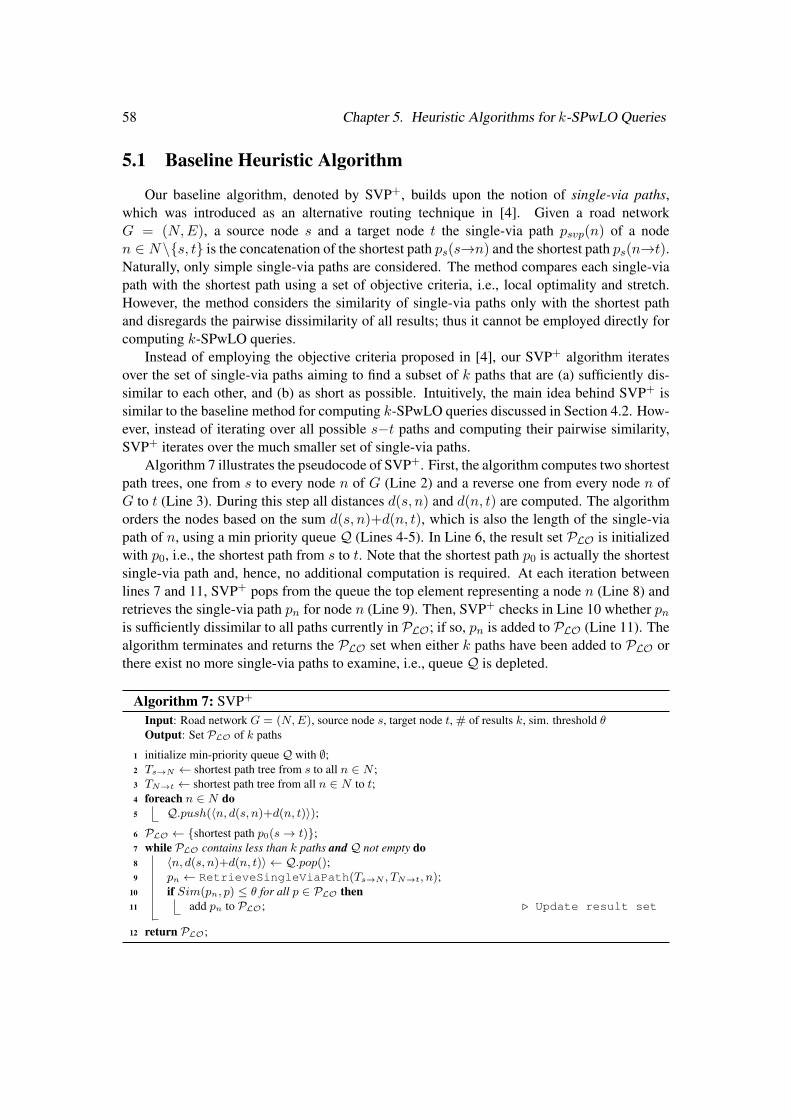
58 Chapter 5. Heuristic Algorithms for k-SPwLO Queries
5.1 Baseline Heuristic Algorithm
Our baseline algorithm, denoted by SVP+, builds upon the notion of single-via paths,which was introduced as an alternative routing technique in [4]. Given a road networkG = (N,E), a source node s and a target node t the single-via path p
svp
(n) of a noden 2 N \{s, t} is the concatenation of the shortest path p
s
(s!n) and the shortest path ps
(n!t).Naturally, only simple single-via paths are considered. The method compares each single-viapath with the shortest path using a set of objective criteria, i.e., local optimality and stretch.However, the method considers the similarity of single-via paths only with the shortest pathand disregards the pairwise dissimilarity of all results; thus it cannot be employed directly forcomputing k-SPwLO queries.
Instead of employing the objective criteria proposed in [4], our SVP+ algorithm iteratesover the set of single-via paths aiming to find a subset of k paths that are (a) sufficiently dis-similar to each other, and (b) as short as possible. Intuitively, the main idea behind SVP+ issimilar to the baseline method for computing k-SPwLO queries discussed in Section 4.2. How-ever, instead of iterating over all possible s�t paths and computing their pairwise similarity,SVP+ iterates over the much smaller set of single-via paths.
Algorithm 7 illustrates the pseudocode of SVP+. First, the algorithm computes two shortestpath trees, one from s to every node n of G (Line 2) and a reverse one from every node n ofG to t (Line 3). During this step all distances d(s, n) and d(n, t) are computed. The algorithmorders the nodes based on the sum d(s, n)+d(n, t), which is also the length of the single-viapath of n, using a min priority queue Q (Lines 4-5). In Line 6, the result set PLO is initializedwith p0, i.e., the shortest path from s to t. Note that the shortest path p0 is actually the shortestsingle-via path and, hence, no additional computation is required. At each iteration betweenlines 7 and 11, SVP+ pops from the queue the top element representing a node n (Line 8) andretrieves the single-via path p
n
for node n (Line 9). Then, SVP+ checks in Line 10 whether pn
is sufficiently dissimilar to all paths currently in PLO; if so, pn
is added to PLO (Line 11). Thealgorithm terminates and returns the PLO set when either k paths have been added to PLO orthere exist no more single-via paths to examine, i.e., queue Q is depleted.
Algorithm 7: SVP+
Input: Road network G = (N,E), source node s, target node t, # of results k, sim. threshold ✓Output: Set PLO of k paths
1 initialize min-priority queue Q with ;;2 T
s!N
shortest path tree from s to all n 2 N ;3 T
N!t
shortest path tree from all n 2 N to t;4 foreach n 2 N do5 Q.push(hn, d(s, n)+d(n, t)i);6 PLO {shortest path p0(s! t)};7 while PLO contains less than k paths and Q not empty do8 hn, d(s, n)+d(n, t)i Q.pop();9 p
n
RetrieveSingleViaPath(Ts!N
, TN!t
, n);10 if Sim(p
n
, p) ✓ for all p 2 PLO then11 add p
n
to PLO; . Update result set
12 return PLO;

5.2. The OnePass+ algorithm 59
Example 5. We demonstrate SVP+ using the road network of Figure 5.1 andthe k-SPwLO(s, t, 0.5, 3) query. First, SVP+ adds the shortest path p(s!t) =
h(s, n3), (n3, n5), (n5, t)i to the result set. Then, SVP+ iterates over the set of single-via pathsin length order. The table in Figure 5.1 shows the entire set of single-via paths for the exampleroad network. The first single-via paths examined are p
svp
(n3) and psvp
(n5). Both paths arerejected as their similarity with the shortest path exceed the similarity threshold ✓. Single-viapaths p
svp
(n3) and psvp
(n5) are the same with the shortest path, hence Sim(psvp
(n3), p) =
Sim(psvp
(n5), p) = 1. In fact, the single-via path of every node on the shortest path is theshortest path. Single-via path p
svp
(n4) is also rejected as Sim(psvp
(n4), p) = 6/8 = 0.75exceeds the similarity threshold. Next, SVP+ examines single-via path p
svp
(n2) for which thesimilarity with the shortest path is Sim(p
svp
(n2), p) = 0. Hence, psvp
(n2) is recommended,i.e., added to the result set. Finally, single-via path p
svp
(n1) is examined for which we haveSim(p
svp
(n1), p) = 3/8 = 0.375 and Sim(psvp
(n1), psvp(n2)) = 0; thus, psvp
(n1) is alsoadded to the result set.
s
n1
n2
n3
n4
n5 t
6
4
3
26
3
5
5
3
12
2
shortest path (p0) 1st alternative (p15) 2nd alternative (p4)
Single-via paths lengthpsvp
(n3) h(s, n3), (n3, n5), (n5, t)i 8psvp
(n5) h(s, n3), (n3, n5), (n5, t)i 8psvp
(n4) h(s, n3), (n3, n5), (n5, n4), (n4, t)i 9psvp
(n2) h(s, n2), (n2, n4), (n4, t)i 11psvp
(n1) h(s, n3), (n3, n1), (n1, t)i 11
Figure 5.1: Example of SVP+.
Notice that in Example 5, SVP+ fails to find the exact result for the given k-SPwLO query.In particular, path p = h(s, n3), (n3, n4), (n4, t)i, which is in the exact k-SPwLO result, is nota single-via path; hence, p is not examined by SVP+.
5.2 The OnePass+ algorithm
Our first heuristic algorithm, denoted by OnePass+, combines the feature of OnePass toscan the road network only once with the pruning power of Lemma 5, which is also used byMultiPass. OnePass+ has the following key features. Given a source node s and a target nodet, OnePass+ traverses the road network expanding every path p(s!n) from source s to a noden that qualifies both Lemma 4 and Lemma 5. This procedure is the same with each distinctround of MultiPass. In contrast to MultiPass though, each time a new path is added to theresult set PLO, an update procedure takes place for all remaining incomplete paths p(s!n).In particular, for every incomplete path p(s!n), OnePass+ computes the overlap of p withthe newly found result and, then, p is checked against Lemma 4 with respect to the updatedPLO. The same update procedure is also employed by OnePass. The algorithm terminates
60 Chapter 5. Heuristic Algorithms for k-SPwLO Queries
when either k paths are added to the result set or all paths from s to t qualifying both Lemma 4and Lemma 5 have been examined.
By not restarting after the computation of each new result, OnePass+ avoids expandingthe network multiple times. However, the fact that OnePass+ does not restart the expansionafter each round implies that the next best path might get pruned. In Section 4.5, we explainedthat for the MultiPass algorithm to find the exact solution, the restart is required. A path that ispruned as non-promising during the current round may be promising during the next round. Allsuch paths are excluded permanently from the search space of OnePass+ and, hence, OnePass+
cannot guarantee that the exact solution is found. Nevertheless, this case applies to only a smallsubset of the examined paths. The average length of paths in the result set of OnePass+ isexpected to be close to the optimal one.
Algorithm 8 illustrates the pseudocode of OnePass+. The algorithm employs a min priorityqueue Q (initialized with source s in Line 1) to traverse the road network. Result set PLO isinitialized with p0, i.e., the shortest path from s to t (Line 2). In between Lines 4 and 21,OnePass+ examines the contents of Q until either k paths are found and added to PLO or Q isdepleted. At each iteration, a label hn, p
n
i is popped from Q (Line 5). If node n is the targett (Line 6), then p
n
is added to PLO (Line 7) and the same update procedure as in OnePasstakes place (Lines 8-10), i.e., all paths p
h
with Sim(ph
, pc
) > ✓ are discarded. Otherwise, thealgorithm expands the current path p
n
considering all outgoing edges (n, nc
) (Lines 12-21).OnePass checks whether the new path p
c
pn
� (n, nc
) qualifies the pruning criteria of bothLemma 4 (Lines 14-15) and Lemma 5 (Lines 16-17) and updates Q and ⇤(n
c
) accordingly.OnePass adds a new label for p
c
to Q (Line 20) and ⇤(nc
) (Line 21) and proceeds with poppingthe next label from Q. Finally, the result set PLO is returned in Line 20.
Similar to OnePass and MultiPass, for each label our implementation of OnePass+ main-tains and updates incrementally a vector V
Sim
containing the overlaps of pn
with all paths thatwhere in PLO at the time when the label was created. Furthermore, OnePass+ also performslazy updates for Q. That is, for labels that have already been created and added to Q, OnePass+
updates VSim
only at the time when a label is popped from Q.
Complexity Analysis Given a k-SPwLO query from a node s to a node t, OnePass+ firstcomputes p0(s!t) using any shortest path algorithm, e.g., Dijkstra, and adds it to the resultset. Naturally, the cost of this step is independent of the number of requested paths k or thesimilarity threshold ✓. To compute alternatives, OnePass+ traverses the road network expand-ing every path p(s!n) from source s to a node n that qualifies both Lemma 4 and Lemma 5.As we discussed in the cost analysis of MultiPass, there can be no formal guarantees regardingthe number of paths that are pruned using either pruning criterion. In the worst case when nopaths are pruned, OnePass+ is equivalent to OnePass and Fox’s algorithm. Therefore, the timecomplexity of OnePass+ is also O(|E|+K · |N | · log |N |), where K is the number of shortestpaths that have to be computed in order to cover the k-SPwLO result.
5.3 Edge Subset Exclusion
Our second heuristic algorithm, denoted by ESX, computes k-SPwLO by iteratively ex-cluding edges from the road network. The idea behind ESX is the following. Given a roadnetwork G = (N,E), a source node s and a target node t, a requested number of paths k and a
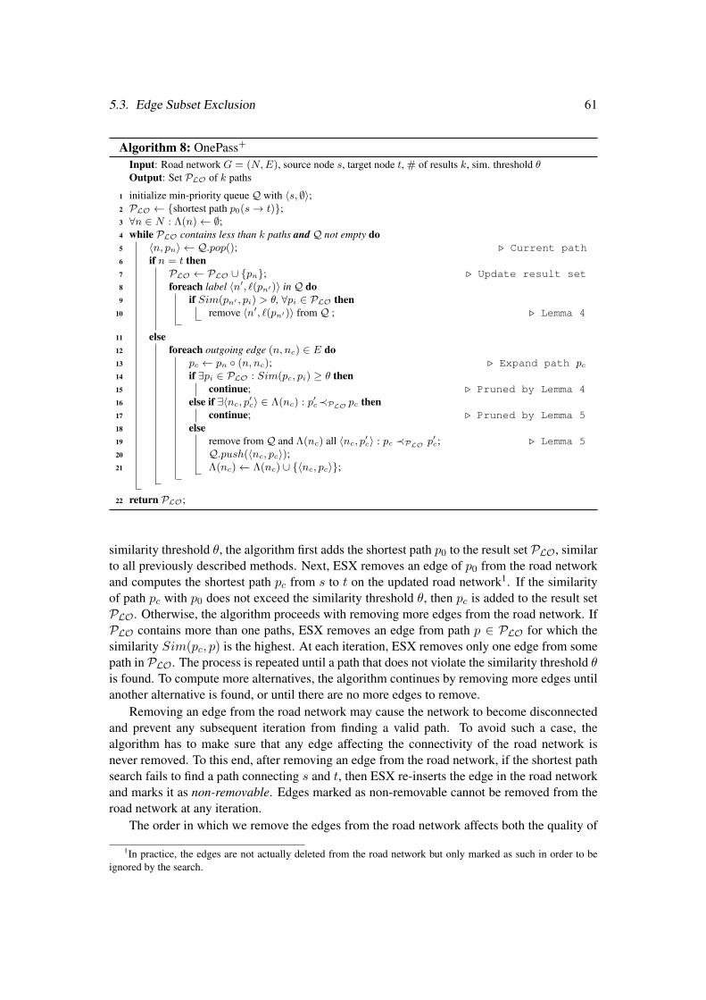
5.3. Edge Subset Exclusion 61
Algorithm 8: OnePass+
Input: Road network G = (N,E), source node s, target node t, # of results k, sim. threshold ✓Output: Set PLO of k paths
1 initialize min-priority queue Q with hs, ;i;2 PLO {shortest path p0(s! t)};3 8n 2 N : ⇤(n) ;;4 while PLO contains less than k paths and Q not empty do5 hn, p
n
i Q.pop(); . Current path6 if n = t then7 PLO PLO [ {p
n
}; . Update result set8 foreach label hn0, `(p
n
0)i in Q do
9 if Sim(pn
0 , pi
) > ✓, 8pi
2 PLO then10 remove hn0, `(p
n
0)i from Q ; . Lemma 4
11 else12 foreach outgoing edge (n, n
c
) 2 E do13 p
c
pn
� (n, nc
); . Expand path pc
14 if 9pi
2 PLO : Sim(pc
, pi
) � ✓ then15 continue; . Pruned by Lemma 416 else if 9hn
c
, p0c
i 2 ⇤(nc
) : p0c
�PLO pc
then17 continue; . Pruned by Lemma 518 else19 remove from Q and ⇤(n
c
) all hnc
, p0c
i : pc
�PLO p0c
; . Lemma 520 Q.push(hn
c
, pc
i);21 ⇤(n
c
) ⇤(nc
) [ {hnc
, pc
i};
22 return PLO;
similarity threshold ✓, the algorithm first adds the shortest path p0 to the result set PLO, similarto all previously described methods. Next, ESX removes an edge of p0 from the road networkand computes the shortest path p
c
from s to t on the updated road network1. If the similarityof path p
c
with p0 does not exceed the similarity threshold ✓, then pc
is added to the result setPLO. Otherwise, the algorithm proceeds with removing more edges from the road network. IfPLO contains more than one paths, ESX removes an edge from path p 2 PLO for which thesimilarity Sim(p
c
, p) is the highest. At each iteration, ESX removes only one edge from somepath in PLO. The process is repeated until a path that does not violate the similarity threshold ✓is found. To compute more alternatives, the algorithm continues by removing more edges untilanother alternative is found, or until there are no more edges to remove.
Removing an edge from the road network may cause the network to become disconnectedand prevent any subsequent iteration from finding a valid path. To avoid such a case, thealgorithm has to make sure that any edge affecting the connectivity of the road network isnever removed. To this end, after removing an edge from the road network, if the shortest pathsearch fails to find a path connecting s and t, then ESX re-inserts the edge in the road networkand marks it as non-removable. Edges marked as non-removable cannot be removed from theroad network at any iteration.
The order in which we remove the edges from the road network affects both the quality of
1In practice, the edges are not actually deleted from the road network but only marked as such in order to beignored by the search.
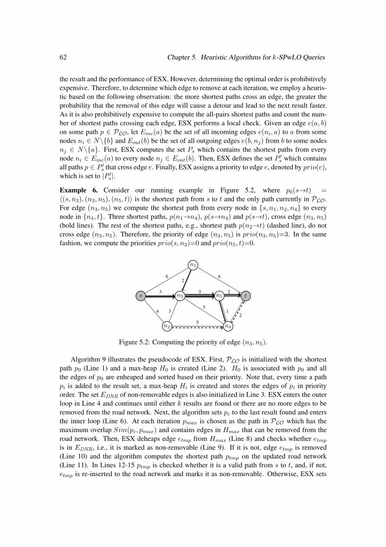
62 Chapter 5. Heuristic Algorithms for k-SPwLO Queries
the result and the performance of ESX. However, determining the optimal order is prohibitivelyexpensive. Therefore, to determine which edge to remove at each iteration, we employ a heuris-tic based on the following observation: the more shortest paths cross an edge, the greater theprobability that the removal of this edge will cause a detour and lead to the next result faster.As it is also prohibitively expensive to compute the all-pairs shortest paths and count the num-ber of shortest paths crossing each edge, ESX performs a local check. Given an edge e(a, b)on some path p 2 PLO, let E
inc
(a) be the set of all incoming edges e(ni
, a) to a from somenodes n
i
2 N\{b} and Eout
(b) be the set of all outgoing edges e(b, nj
) from b to some nodesnj
2 N\{a}. First, ESX computes the set Ps
which contains the shortest paths from everynode n
i
2 Einc
(a) to every node nj
2 Eout
(b). Then, ESX defines the set P 0s
which containsall paths p 2 P 0
s
that cross edge e. Finally, ESX assigns a priority to edge e, denoted by prio(e),which is set to |P 0
s
|.Example 6. Consider our running example in Figure 5.2, where p0(s!t) =
h(s, n3), (n3, n5), (n5, t)i is the shortest path from s to t and the only path currently in PLO.For edge (n3, n5) we compute the shortest path from every node in {s, n1, n2, n4} to everynode in {n4, t}. Three shortest paths, p(n1!n4), p(s!n4) and p(s!t), cross edge (n3, n5)
(bold lines). The rest of the shortest paths, e.g., shortest path p(n2!t) (dashed line), do notcross edge (n3, n5). Therefore, the priority of edge (n3, n5) is prio(n3, n5)=3. In the samefashion, we compute the priorities prio(s, n3)=0 and prio(n5, t)=0.
s
n1
n2
n3
n4
n5 t
6
4
3
26
3
5
5
3
12
2
Figure 5.2: Computing the priority of edge (n3, n5).
Algorithm 9 illustrates the pseudocode of ESX. First, PLO is initialized with the shortestpath p0 (Line 1) and a max-heap H0 is created (Line 2). H0 is associated with p0 and allthe edges of p0 are enheaped and sorted based on their priority. Note that, every time a pathpi
is added to the result set, a max-heap Hi
is created and stores the edges of pi
in priorityorder. The set E
DNR
of non-removable edges is also initialized in Line 3. ESX enters the outerloop in Line 4 and continues until either k results are found or there are no more edges to beremoved from the road network. Next, the algorithm sets p
c
to the last result found and entersthe inner loop (Line 6). At each iteration p
max
is chosen as the path in PLO which has themaximum overlap Sim(p
c
, pmax
) and contains edges in Hmax
that can be removed from theroad network. Then, ESX deheaps edge e
tmp
from Hmax
(Line 8) and checks whether etmp
is in EDNR
, i.e., it is marked as non-removable (Line 9). If it is not, edge etmp
is removed(Line 10) and the algorithm computes the shortest path p
tmp
on the updated road network(Line 11). In Lines 12-15 p
tmp
is checked whether it is a valid path from s to t, and, if not,etmp
is re-inserted to the road network and marks it as non-removable. Otherwise, ESX sets

5.3. Edge Subset Exclusion 63
pc
to ptmp
and proceeds to the next iteration. When the inner loop is finished, the algorithmchecks if p
c
is a valid alternative path by checking its similarity with all paths currently in PLO(Line 17). If p
c
is a valid alternative, it is added to PLO and a new max-heap Hc
associatedwith p
c
is initialized with the edges of pc
(Lines 18-19). Finally, after the outer loop is finished,the result set PLO is returned in Line 20.
Algorithm 9: ESXInput: Road network G(N,E), source node s, target node t, # of results k, sim. threshold ✓Output: Set PLO of k paths
1 PLO {shortest path p0(s! t)};2 initialize max-heap H0 hei,prio(G, e
i
)i, 8ei
2 p0; . Hi
is associated with pi
3 initialize EDNR
;;4 while PLO contains less than k paths and 9H
i
not empty do5 set p
c
last path added to PLO;6 while max{Sim(p
c
, pi
) : pi
2 PLO and Hi
not empty } > ✓ do7 Edge e
tmp
Hi
.pop();8 if e
tmp
2 EDNR
then9 continue;
10 G.remove(etmp
);11 Path p
tmp
ShortestPath(G, s, t);12 if p
tmp
is null then13 re-insert e
tmp
to G;14 insert e
tmp
to EDNR;15 continue;
16 pc
ptmp
;
17 if max{Sim(pc
, pi
) : pi
2 PLO} then18 add p
c
to PLO;19 initialize max-heap H
c
hej
,prio(G, ej
)i, 8ej
2 pc
;
20 return PLO;
Example 7. We demonstrate the functionality of ESX using the road network of Figure 5.2and the k�SPwLO(s, t, 0.5, 2) query. During initialization, the shortest path p0(s!t) =
h(s, n3), (n3, n5), (n5, t)i is computed and added to the result set PLO. Next, we com-pute the priority of each edge of the shortest path. Having computed the priorities, wefirst remove edge (n3, n5), which is the edge with the highest priority. Then, we computethe shortest path p0(s!t) on the updated road network. The shortest path is p0(s!t) =
h(s, n3), (n3, n4), (n4, t)i with `(p0(s!t)) = 10. We check the overlap of the new path withthe original shortest path and find that Sim(p0(s!t), p0) = 0.375, which does not exceed thesimilarity threshold. Therefore, p0(s!t) is added to PLO.
Complexity Analysis ESX reduces the search for an alternative path to a set of ordinaryshortest path queries. In particular, given a road network G = (N,E) let PLO be the result setof a k-SPwLO(s, t, ✓, k) query containing k paths. ESX requires |P |⇥ total number of edgesin P executions of shortest path queries, i.e., the number of shortest path queries that have tobe processed is linear to the number k of paths and the size of the result paths.
Finally, in our implementation of ESX we employed the optimization using lower boundsdescribed in Section 4.6, which reduces the cost for retrieving shortest paths and optimizes the
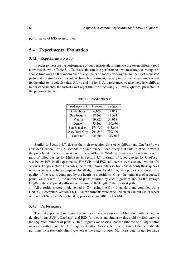
64 Chapter 5. Heuristic Algorithms for k-SPwLO Queries
performance of ESX even further.
5.4 Experimental Evaluation
5.4.1 Experimental Setup
In order to measure the performance of our heuristic algorithms we use seven different roadnetworks shown in Table 5.1. To assess the runtime performance, we measure the average re-sponse time over 1,000 random queries (i.e., pairs of nodes), varying the number k of requestedpaths and the similarity threshold ✓. In each experiment, we vary one of the two parameters andfix the other to its default value: 3 for k and 0.5 for ✓. As a reference, we also include MultiPassin our experiments, the fastest exact algorithm for processing k-SPwLO queries, presented inthe previous chapter.
Table 5.1: Road networks.
road network # nodes # edgesOldenburg 6,105 14,058
San Joaquin 18,263 47,594Vienna 19,826 54,918Denver 73,166 196,630
San Francisco 174,956 443,604New York City 264,346 730,100
Colorado 435,666 1,057,066
Similar to Section 4.7, due to the high execution time of MultiPass and OnePass+, weconsider a timeout of 120 seconds for each query. Each query that fails to execute withinthe predefined timeout is considered timed-out/failed. While we have already reported on theratio of failed queries for MultiPass in Section 4.7, the ratio of failed queries for OnePass+
was below 10% in all experiments. For SVP+ and ESX, all queries were executed within 120seconds. For presentation purposes, the results shown in this section consider only those querieswhich were successfully completed by all algorithms. In addition, we report experiments on thequality of the results computed by the heuristic algorithms. Given the number k of requestedpaths, we measure (a) the number of paths returned by each algorithm and (b) the averagelength of the computed paths in comparison to the length of the shortest path.
All algorithms were implemented in C++ using the C++11 standard and compiled usingGNU G++ compiler (version 4.8.1). All experiments were executed on an Ubuntu Linux serverwith 4 Intel Xeon X5550 (2.67GHz) processors and 48GB of RAM.
5.4.2 Performance
The first experiment in Figure 5.3 compares the exact algorithm MultiPass with the heuris-tic algorithms SVP+, OnePass+ and ESX for a constant similarity threshold ✓=50% varyingthe requested number of paths k. In all figures we observe that the runtime of all algorithmsincreases with the number k of requested paths. As expected, the runtime of the heuristic al-gorithms increases only slightly, whereas the exact solution MultiPass deteriorates for large

5.4. Experimental Evaluation 65
2 3 4 5
0
1
2
3
4
k
Res
pons
etim
e(s
ec)
MultiPass OnePass+ ESX SVP+
(a) Oldenburg
2 3 4 5
0
2
4
6
8
10
k
Res
pons
etim
e(s
ec)
(b) San Joaquin
2 3 4 5
0
1
2
3
4
5
k
Res
pons
etim
e(s
ec)
(c) Vienna
2 3 4 5
0
2
4
6
8
k
Res
pons
etim
e(s
ec)
(d) Denver
Figure 5.3: Performance comparison of algorithms varying requested paths k (✓=50%).
values of k. For k>3, MultiPass becomes one order of magnitude slower than OnePass+ andmore than two orders of magnitude slower than ESX and SVP+. Clearly, MultiPass cannotscale and, hence, we exclude it from our measurements on Vienna and Denver (Figures 5.3c-d). Furthermore, in Figures 5.3c-d we also observe that the performance of OnePass, SVP+ andESX is similar. However, for increasing values of k both SVP+ and ESX clearly outperformOnePass+ up two one order of magnitude.
The second experiment compares the exact algorithm MultiPass with the heuristic algo-rithms SVP+, OnePass+ and ESX for a constant requested number of paths k=3 varying thesimilarity threshold ✓. Figure 5.4 shows that for ✓<70%, MultiPass is much slower than theheuristic algorithms: one order of magnitude slower than OnePass+ and two orders of mag-nitude slower than SVP+ and ESX (for ✓=30%). For large values of ✓, the performance ofMultiPass gets closer to the performance of the heuristic algorithms (for ✓=90% MultiPassis even faster than ESX and SVP+). We also observe that OnePass+ is very fast for extremevalues of ✓ (✓=10% and ✓=90%), but it is rather slow for values in between.
Another interesting observation in Figures 5.3c–d and 5.4c–d is that the performance ofMultiPass and OnePass+ shows a local maximum for ✓=30%, which indicates the followingimportant trade-off. As ✓ increases, the pruning power of Lemma 4 deteriorates, and bothMultiPass and OnePass+ construct more paths. At the same time, the next result will be de-termined earlier, and hence the total runtime drops. In addition, as ✓ decreases, the pruningpower of Lemma 5 increases and more partial paths can be pruned. This explains the behaviorof MultiPass and OnePass+, where the response time initially increases, but after ✓=30% theruntime of both algorithms goes down again.
To sum up, the heuristic algorithms clearly outperform the correct algorithm MultiPass.Comparing the heuristic algorithms, we observe that SVP+ and ESX have a similar perfor-mance and are the clear winners for small and medium size datasets. Apparently, OnePass+ is
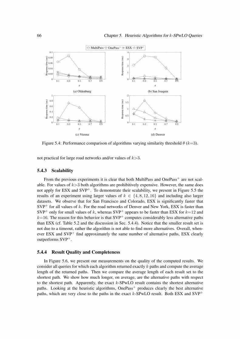
66 Chapter 5. Heuristic Algorithms for k-SPwLO Queries
0.1 0.3 0.5 0.7 0.90
0.02
0.04
0.06
0.08
0.1
✓
Res
pons
etim
e(s
ec)
MultiPass OnePass+ ESX SVP+
(a) Oldenburg
0.1 0.3 0.5 0.7 0.90
1
2
3
4
✓
Res
pons
etim
e(s
ec)
(b) San Joaquin
0.1 0.3 0.5 0.7 0.90
0.2
0.4
0.6
0.8
1
✓
Res
pons
etim
e(s
ec)
(c) Vienna
0.1 0.3 0.5 0.7 0.90
0.5
1
1.5
2
✓
Res
pons
etim
e(s
ec)
(d) Denver
Figure 5.4: Performance comparison of algorithms varying similarity threshold ✓ (k=3).
not practical for large road networks and/or values of k>3.
5.4.3 Scalability
From the previous experiments it is clear that both MultiPass and OnePass+ are not scal-able. For values of k>3 both algorithms are prohibitively expensive. However, the same doesnot apply for ESX and SVP+. To demonstrate their scalability, we present in Figure 5.5 theresults of an experiment using larger values of k 2 {4, 8, 12, 16} and including also largerdatasets. We observe that for San Francisco and Colorado, ESX is significantly faster thatSVP+ for all values of k. For the road networks of Denver and New York, ESX is faster thanSVP+ only for small values of k, whereas SVP+ appears to be faster than ESX for k=12 andk=16. The reason for this behavior is that SVP+ computes considerably less alternative pathsthan ESX (cf. Table 5.2 and the discussion in Sec. 5.4.4). Notice that the smaller result set isnot due to a timeout, rather the algorithm is not able to find more alternatives. Overall, when-ever ESX and SVP+ find approximately the same number of alternative paths, ESX clearlyoutperforms SVP+.
5.4.4 Result Quality and Completeness
In Figure 5.6, we present our measurements on the quality of the computed results. Weconsider all queries for which each algorithm returned exactly k paths and compute the averagelength of the returned paths. Then we compare the average length of each result set to theshortest path. We show how much longer, on average, are the alternative paths with respectto the shortest path. Apparently, the exact k-SPwLO result contains the shortest alternativepaths. Looking at the heuristic algorithms, OnePass+ produces clearly the best alternativepaths, which are very close to the paths in the exact k-SPwLO result. Both ESX and SVP+

5.4. Experimental Evaluation 67
4 8 8 12 12 16 160
2
4
6
8
10
12
k
Res
pons
etim
e(s
ec)
ESX SVP+
(a) Denver
4 8 8 12 12 16 160
10
20
30
40
k
Res
pons
etim
e(s
ec)
(b) San Francisco
4 8 8 12 12 16 160
10
20
30
40
50
k
Res
pons
etim
e(s
ec)
(c) New York
4 8 8 12 12 16 160
100
200
300
k
Res
pons
etim
e(s
ec)
(d) Colorado
Figure 5.5: Performance comparison of SVP+ and ESX for k 2 {2, 4, 8, 16} and ✓ = 50%.
recommend alternative paths that are, on average, up to 15% longer than the alternative pathsin k-SPwLO. The alternative paths recommended by ESX, though, are most of the time shorterthan the alternative paths recommended by SVP+.
2 3 4 5
0
5
10
15
20
25
k
Diff
.with
sp(%
)
k-SPwLO OnePass+ ESX SVP+
(a) Oldenburg
2 3 4 5
0
5
10
15
20
k
Diff
.with
sp(%
)
(b) San Joaquin
2 3 4 5
0
2
4
6
8
10
k
Diff
.with
sp(%
)
(c) Vienna
2 3 4 5
0
5
10
15
20
25
k
Diff
.with
sp(%
)
(d) Denver
Figure 5.6: Result quality of algorithms varying requested paths k (✓ = 50%).
Next, we measure the completeness of the result sets. Table 5.2 reports for each algorithmthe percentage of queries for which exactly k alternative paths were found. Apparently, theexact solution k-SPwLO has the highest completion ratio. The completion ratio OnePass+ is
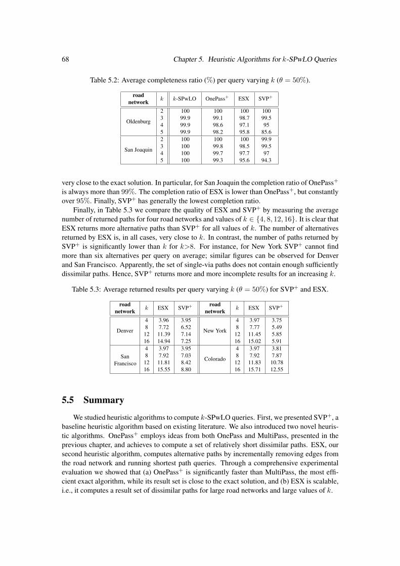
68 Chapter 5. Heuristic Algorithms for k-SPwLO Queries
Table 5.2: Average completeness ratio (%) per query varying k (✓ = 50%).
roadk k-SPwLO OnePass+ ESX SVP+
network
Oldenburg
2 100 100 100 1003 99.9 99.1 98.7 99.54 99.9 98.6 97.1 955 99.9 98.2 95.8 85.6
San Joaquin
2 100 100 100 99.93 100 99.8 98.5 99.54 100 99.7 97.7 975 100 99.3 95.6 94.3
very close to the exact solution. In particular, for San Joaquin the completion ratio of OnePass+
is always more than 99%. The completion ratio of ESX is lower than OnePass+, but constantlyover 95%. Finally, SVP+ has generally the lowest completion ratio.
Finally, in Table 5.3 we compare the quality of ESX and SVP+ by measuring the averagenumber of returned paths for four road networks and values of k 2 {4, 8, 12, 16}. It is clear thatESX returns more alternative paths than SVP+ for all values of k. The number of alternativesreturned by ESX is, in all cases, very close to k. In contrast, the number of paths returned bySVP+ is significantly lower than k for k>8. For instance, for New York SVP+ cannot findmore than six alternatives per query on average; similar figures can be observed for Denverand San Francisco. Apparently, the set of single-via paths does not contain enough sufficientlydissimilar paths. Hence, SVP+ returns more and more incomplete results for an increasing k.
Table 5.3: Average returned results per query varying k (✓ = 50%) for SVP+ and ESX.
roadk ESX SVP+ road
k ESX SVP+
network network
Denver
4 3.96 3.95
New York
4 3.97 3.758 7.72 6.52 8 7.77 5.4912 11.39 7.14 12 11.45 5.8516 14.94 7.25 16 15.02 5.91
SanFrancisco
4 3.97 3.95
Colorado
4 3.97 3.818 7.92 7.03 8 7.92 7.8712 11.81 8.42 12 11.83 10.7816 15.55 8.80 16 15.71 12.55
5.5 Summary
We studied heuristic algorithms to compute k-SPwLO queries. First, we presented SVP+, abaseline heuristic algorithm based on existing literature. We also introduced two novel heuris-tic algorithms. OnePass+ employs ideas from both OnePass and MultiPass, presented in theprevious chapter, and achieves to compute a set of relatively short dissimilar paths. ESX, oursecond heuristic algorithm, computes alternative paths by incrementally removing edges fromthe road network and running shortest path queries. Through a comprehensive experimentalevaluation we showed that (a) OnePass+ is significantly faster than MultiPass, the most effi-cient exact algorithm, while its result set is close to the exact solution, and (b) ESX is scalable,i.e., it computes a result set of dissimilar paths for large road networks and large values of k.

CHAPTER 6
MoTrIS: A System for Multimodal Route Planning
In this chapter, we present MoTrIS, a Multimodal Transport Information System. MoTrISdiffers from existing frameworks as it not only offers route planning services over road net-works, but also tackles the challenge of combining different types of networks into a singlemultimodal network. MoTrIS allows shortest path and distance query processing on multi-modal transportation networks. Such fundamental queries can be employed as basic buildingblocks for creating advanced solutions to different types of problems on multimodal networks,e.g., journey and itinerary planning. Selected algorithms presented in the previous chaptersof this thesis for route planning on road networks, have been implemented and integrated intoMoTrIS as well.
69

70 Chapter 6. MoTrIS: A System for Multimodal Route Planning
6.1 MoTrIS Framework
MoTrIS is a service-oriented framework designed to support applications that depend onmultimodal transportation networks. The framework allows users/developers to create cus-tomized services over specific regions. First, the users choose a road network and select themodes of transportation which will be associated with the selected road network. Then, MoTrIScreates a new instance/service where the selected street and transportation networks are com-bined into a single multimodal network. To enable easy access to query services, MoTrISprovides an API which allows users to employs the customized routing services directly intheir applications.
6.1.1 System Overview
Figure 6.1 illustrates the architecture of MoTrIS, which is composed of four core mod-ules: the network module represents the multimodal network; the timetable module handlesthe transportation network data, i.e., the schedule and the availability of each transportationmode; the query processing module includes algorithms for processing queries either on themultimodal network or on each of its individual components; and the visualization moduleproduces the results of each query execution.
Apart from the core modules, Figure 6.1 also illustrates the data import, which is re-sponsible for importing road and transportation network data into PostGIS1, a spatial-enabledRDBMS, as well as the web application, which allows users to create new services and runsample queries to test the services.
AP
I
QueryProcessing
Timetable
Visualization
Network
WebApplication
API Calls
Data ImportPostGIS
mExternal Sources (osm, gtfs)
Figure 6.1: System architecture.
6.1.2 Data Import and PostGIS
The data import module is responsible for importing road and transportation network datafrom various sources into PostGIS. In particular, we obtain road network data from Open-StreetMap2 (OSM). The road network data from OSM is then transformed into a routable graphformat and stored in a single relational table in PostGIS. Each tuple represents an edge of theroad network along with related information about the edge and its two adjacent nodes, i.e.,
1http://postgis.net2https://www.openstreetmap.org/

6.1. MoTrIS Framework 71
edge length, source and target node location, etc. Together with the road network, a polygonthat marks the boundaries of the region associated with the road network is stored in PostGIS.
Routing services can be employed over any imported region directly. To employ servicesover smaller regions though, the module allows users to specify sub-regions of already importedregions. Polygons representing sub-regions are stored in PostGIS in a hierarchical fashion,as illustrated in Figure 6.2. Note that in order to define a sub-region, the polygon boundingthe sub-region must entirely inside the polygon bounding an already imported region. Afterspecifying a polygon that represents a sub-region, the module extracts the edges of the roadnetwork that lie inside the given polygon. Then, PostGIS creates a view which models only thepart of the road network that is bounded by the given polygon3.
Figure 6.2 illustrates an example, where we have the entire network of Italy obtained fromOSM and stored in table italy streets. The polygons representing various cities and states arestored in table road network. To obtain the road network for the city of Bolzano, all the edgesthat lie entirely inside the respective polygon are extracted. Then, the view bolzano view iscreated which contains only the edges on the sub-network for the city of Bolzano.
Note that the extracted edges may not always form a connected road network but may formseveral ones. Since sub-regions are not always defined with the road network in mind, it ispossible that, in order to reach certain parts of the bounded region, the user has to travel outsidethe region first. To address this problem, the data import module comes with an optionalverification process which extracts only the largest sub-network and, hence, ensures that theroad network of every sub-region is a connected graph.
Italy
Veneto
Verona
South Tyrol
Merano Bolzano
italy streetsid src trg length geometry1 1 2 254 linestr 12 1 3 128 linestr 23 2 1 254 linestr 34 2 4 365 linestr 45 3 1 129 linestr 56 4 5 241 linestr 67 5 4 243 linestr 7
road networkid region boundary pid1 italy polygon 1 -2 s tyrol polygon 2 13 veneto polygon 3 14 merano polygon 4 25 bolzano polygon 5 26 verona polygon 6 3
bolzano viewid src trg length1 1 2 2542 1 3 1283 2 1 2544 2 4 3655 3 1 128
Figure 6.2: Sub-region road network extraction.
For transportation network data, we first create a set of relational tables in PostGIS thatmatch the General Transit Feed Specification4 (GTFS). We outline the key GTFS entities forbuilding a transportation network: stops, which are individual locations where vehicles pick upor drop off passengers and can be associated with several routes; routes, which are groups oftrips that are displayed to riders as a single transportation service, i.e., a bus line; trips, which
3In practice, instead of creating a view, we add a column of Bit type to the table storing the road network tomark the edges that are on the road network of the sub-region.
4https://developers.google.com/transit/gtfs/reference

72 Chapter 6. MoTrIS: A System for Multimodal Route Planning
BUS STOP
AB
C
u v
Route ARoute BRoute CRoad Network
p
Figure 6.3: Multimodal network.
store sequences of two or more stops that are on the same route; and stop times, which storethe time that a vehicle arrives at and departs from individual stops for each trip. The modulecreates additional columns for spatial data types. For example, the location of a stop is storedboth as two separate float numbers (representing longitude and latitude as dictated by GTFS)and as a Point data type.
Finally, the data import module associates each imported transportation network with analready imported (or extracted) road network. The associated road network is either providedmanually or is determined automatically as the network bounded by the smallest polygon whichalso bounds the given transportation network. For each stop in the transportation network, theclosest point p of the road network (the black point along the road network in Figure 6.3)is computed and edge e(u, v) which contains p is retrieved. Weights w
u
(u, p) and wv
(p, v),which represent the length of the segment of e from u to point p and the length of the segmentof e from point p to v, respectively, are determined. Finally, two links for each bus stop arestored as a single tuple hstop id, e id, u node id, v node id, w
u
, wv
i in PostGIS.Since the regions are stored hierarchically, the transportation network associated with a
given region can be directly employed for services on all the ancestors of the given region inthe hierarchy. For example, given the polygon hierarchy in Figure 6.2, a transportation networkassociated with Bolzano can be directly employed for services over South Tyrol and Italy.
6.1.3 Network Model
The network module is responsible for constructing and maintaining the multimodal net-work graph for each service in main memory. To construct a multimodal network, we firstchoose a region and the module obtain from the database the road network for the selectedregion. Then, the module loads from PostGIS the transportation networks selected by the userand models each transportation network following the time-dependent model [69]. For allroutes, the stops that each route serves are extracted from the trips. For each distinct pair of aroute and a stop, a node is created and added to the transportation network graph. For example,in Figure 6.3 there are three routes passing through the bus stop. Hence, there are three nodesA, B and C, one for each route, added to the transportation network graph. Subsequently, themodule extracts from the trips all pairs of consecutive stops. An edge connecting nodes thatare associated with consecutive stops and are on the same route, is added to the transportationnetwork graph. Each edge is assigned with a travel time function, which is executed on querytime and determines the weight, i.e., the time required to cross the edge.

6.1. MoTrIS Framework 73
Next, transfer link edges between nodes of the transportation network are generated toallow transfers. Apparently, a stop can be associated with more than one nodes. The numberof nodes associated with a given stop is the same as the number of routes that pass through thatstop. The module adds transfer link edges between all nodes associated with the same stop (reddashed lines in Figure 6.3). The weight of each link edge represents the time required to switchfrom one route to another. By default the transfer time is zero, unless it is specified explicitlyin the input GTFS timetable.
Finally, for each bus stop, the module loads from the database the precomputed links tonodes u and v of the road network. For each node n associated with a stop, two link edgese(u, n) and e(n, v) with weights w
u
and wv
, respectively, are added to the network graph,thereby connecting the transportation networks with the road network. In Figure 6.3, each ofthe two blue/dashed lines represents three link edges, each connecting a road network nodewith one of the nodes A, B, C of the transportation network, all associated with the same stop.
6.1.4 Timetable
The timetable module is responsible for storing in main memory and querying the scheduleof each transportation network. Given a timestamp and an edge of some transportation network,the timetable determines the weight of the edge, i.e., the time needed to cross the edge at thegiven timestamp. For example, given a bus network, the timetable module stores for each edgee a set of entries {n
s
, nd
, ts
, td
}, where ns
is the source node, nd
is the target node, ts
is thedeparture time of the bus from the stop associated with n
s
and td
is the arrival time of the busat the stop associated with n
t
. Given a timestamp t, i.e., arrival time of the user at the stopassociated with n
s
, the timetable determines the bus that the user should take to reach nd
. Theselected bus is the one which arrives at the stop after t, i.e., t
s
� t and the travel time td
� trequired to reach node n
d
, which also includes the waiting time, is minimum.
6.1.5 Query Processing
The query processing module executes queries over the multimodal network. Shortest pathqueries are of the form q(G, p
s
, pt
, t), where G is a multimodal network, ps
and pt
are thesource and destination query points on the map and t is the starting time of the journey. First,the module maps the query points to the multimodal network in the same way bus stops aremapped during the construction of the network. To compute the shortest path on the multimodalnetwork, a modified version of Dijkstra’s algorithm is used. During the expansion of edges onthe road network, the fixed weight is used, whereas during the expansion of edges on sometransportation network, the module queries the timetable to obtain the weights of the edges.
Apart from route planning on multimodal networks, the query processing module can alsoprocess queries over the road network by simply ignoring transportation and link edges. Forprocessing queries over the road network, we have implemented and integrated into MoTrIStwo of our algorithms: (a) ParDiSP, for processing distance and shortest path queries, and (b)ESX, for recommending alternative routes.
We have designed the query processing module in a way that it is highly extensible; newalgorithmic implementations can be integrated easily into our framework. Algorithms in thequery processing module can be accessed via a public API interface, which provides the userswith all the required calls for submitting queries and retrieve results. The multimodal network

74 Chapter 6. MoTrIS: A System for Multimodal Route Planning
is accessed in an abstract way and cannot be modified by the algorithms that are implemented inthe query processing module. By designing the module with extensibility in mind, we aim forMoTrIS to become a solid framework for further research that is not limited to route planningservices on multimodal networks. More algorithms for processing different types of queriescan be added to our framework, as long as the implementation of these algorithms does notrequire the modification of the network model.
6.1.6 Visualization
The visualization module is responsible for producing the results in a visualizable formatafter a query is successfully executed. Given the result of a shortest path query, first the moduleretrieves from the network model the geometries for all the edges contained in the shortest path.Then a response in GeoJSON5 format is generated, which can be visualized directly by mostexternal map services, e.g., Google Maps, Mapbox, OpemStreetMap, etc. Apart from the routeitself, the module includes in the GeoJSON response additional information about the result,such as distance, trip duration for each mode, cost of the trip, etc., provided that the informationis available in the dataset.
6.1.7 Web Application
The web application allows users to create, modify and test services. Users can create anew service by selecting the region/road network on which their service will be applied, thetransportation modes that will be supported by the new service and the queries that will beavailable. The application allows the visualization of the resulting multimodal network. Foreach route in the transportation network, the application also displays the links connecting thetransportation network stops with the street network.
Moreover, to get a clear picture of the query results, a testing interface which uses the APIfor submitting queries and visualizing the results is provided. The testing interface providesall the necessary tools to allow users to explore the functionality of the public API, along withinstructions on how to access the API directly from external applications. For the visualizationthe module employs Mapbox6.
6.2 Use-cases
This section present the main use-cases of our MoTrIS framework. We split the users ofMoTrIS into two groups:
• the administrators who manage existing data and import new data into PostGIS, and
• the developers who want to use our framework for building customized routing servicesand employ them in their applications
In what follows, we present use-cases for both user groups.
5http://geojson.org6https://www.mapbox.com
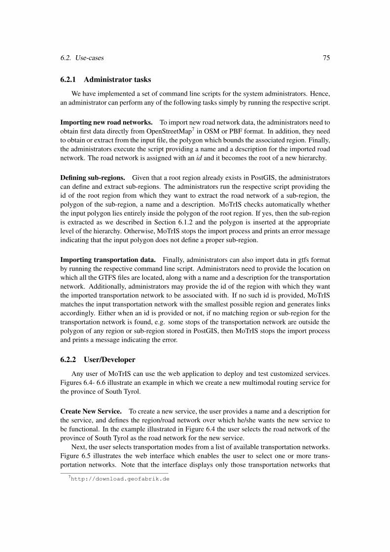
6.2. Use-cases 75
6.2.1 Administrator tasks
We have implemented a set of command line scripts for the system administrators. Hence,an administrator can perform any of the following tasks simply by running the respective script.
Importing new road networks. To import new road network data, the administrators need toobtain first data directly from OpenStreetMap7 in OSM or PBF format. In addition, they needto obtain or extract from the input file, the polygon which bounds the associated region. Finally,the administrators execute the script providing a name and a description for the imported roadnetwork. The road network is assigned with an id and it becomes the root of a new hierarchy.
Defining sub-regions. Given that a root region already exists in PostGIS, the administratorscan define and extract sub-regions. The administrators run the respective script providing theid of the root region from which they want to extract the road network of a sub-region, thepolygon of the sub-region, a name and a description. MoTrIS checks automatically whetherthe input polygon lies entirely inside the polygon of the root region. If yes, then the sub-regionis extracted as we described in Section 6.1.2 and the polygon is inserted at the appropriatelevel of the hierarchy. Otherwise, MoTrIS stops the import process and prints an error messageindicating that the input polygon does not define a proper sub-region.
Importing transportation data. Finally, administrators can also import data in gtfs formatby running the respective command line script. Administrators need to provide the location onwhich all the GTFS files are located, along with a name and a description for the transportationnetwork. Additionally, administrators may provide the id of the region with which they wantthe imported transportation network to be associated with. If no such id is provided, MoTrISmatches the input transportation network with the smallest possible region and generates linksaccordingly. Either when an id is provided or not, if no matching region or sub-region for thetransportation network is found, e.g. some stops of the transportation network are outside thepolygon of any region or sub-region stored in PostGIS, then MoTrIS stops the import processand prints a message indicating the error.
6.2.2 User/Developer
Any user of MoTrIS can use the web application to deploy and test customized services.Figures 6.4- 6.6 illustrate an example in which we create a new multimodal routing service forthe province of South Tyrol.
Create New Service. To create a new service, the user provides a name and a description forthe service, and defines the region/road network over which he/she wants the new service tobe functional. In the example illustrated in Figure 6.4 the user selects the road network of theprovince of South Tyrol as the road network for the new service.
Next, the user selects transportation modes from a list of available transportation networks.Figure 6.5 illustrates the web interface which enables the user to select one or more trans-portation networks. Note that the interface displays only those transportation networks that
7http://download.geofabrik.de

76 Chapter 6. MoTrIS: A System for Multimodal Route Planning
Figure 6.4: Selection of road the transportation networks.
are compatible with the selected road network. Therefore, the only available transportationnetwork shown in Figure 6.5 is that of SASA, the local city-bus company.
Figure 6.5: Selection of road the transportation networks.
After the user has verified his selection, MoTrIS extracts from the database the road net-work for the requested region as well as the timetables for the requested transportation net-works, and constructs the multimodal network for the new service. The new service is loadedinto the main memory and is ready to be accessed using the API.
Run Sample Queries. Next, we show how the user can submit shortest path queries toMoTrIS and visualize the results using the web interface. The application asks the user todefine a starting location, a destination, the date and the starting time (or the desirable arrivaltime) of his trip. Figure 6.6 illustrates the web interface of MoTrIS for testing query services.More specifically, the visualization of a shortest path query over a multimodal network for thecity of Bolzano is shown. The blue lines represent the parts of the route that the user crosseson foot while the orange lines represent the parts that are crossed by bus.
6.3. Summary 77
Figure 6.6: Sample query result visualization.
6.3 Summary
We presented MoTrIS, a service-oriented framework which provides support for buildingapplications on multimodal networks. Our framework combines street and transportation net-works into a single multimodal network and provides query services via a public API. Apartfrom route planning on multimodal transportation networks, MoTrIS can also be employedfor route planning on road networks. Selected algorithms presented in the previous chaptersof the thesis for route planning and alternative routing, have been integrated into MoTrIS aswell. MoTrIS comes with a web-interface which enables users to create, modify and test theirown customized services. Last but not least, MoTrIS was implemented with extensibility inmind; thus, more algorithms for processing different types of queries can be implemented andintegrated into our framework easily.


CHAPTER 7
Conclusion
7.1 Summary
In this thesis, we studied, formalized and proposed algorithmic solutions for two problemsrelated to route planning on road networks: the processing of distance and shortest path queriesand the computation of dissimilar yet short alternative paths.
For processing distance and shortest path queries on road networks, we presented ParDiSP,a framework which supports the efficient processing of both types of queries. We showed howParDiSP partitions the network into components and precomputes a set of index structures.Distance and shortest path queries are processed by running the ALT [38] algorithm if sourceand target are in the same component. Otherwise, for distance queries ParDiSP combinesdistances from three precomputed tables, whereas shortest path queries are decomposed intothe retrieval of three sub-paths, which can be executed in parallel. An experimental evaluationhas shown that ParDiSP outperforms the state-of-the-art for shortest path queries, while beingcomparable to the state-of-the-art for distance queries. For mixed query sets containing bothdistance and shortest path queries, ParDiSP is even more efficient than a combination of thebest state-of-the-art approaches for the two query types, while incurring less space overhead.
The second problem we studied is that of alternative routing on road networks. Our goalwas to recommend k paths that are sufficiently dissimilar to each other and as short as possible.We formalized this task using the k-Shortest Path with Limited Overlap query. We also de-signed and implemented three algorithms for processing k-SPwLO queries: BSL builds uponthe computation of the K�shortest paths; OnePass traverses the network once expanding onlypaths that do not violate the similarity constraint; and MultiPass progressively computes theresult set after traversing the network k�1 times, while employing two powerful pruning crite-ria. Through an extensive experimental evaluation, we demonstrated that MultiPass is the mostefficient algorithm for processing k-SPwLO queries outperforming its competitors and, in mostcases, by a large margin.
To achieve scalability though, we also introduced two heuristic algorithms. OnePass+
employs ideas from both OnePass and MultiPass and achieves to compute a set of dissimilar
79
80 Chapter 7. Conclusion
paths which, in terms of average length, is very close to the exact solution. ESX computesalternative paths by incrementally removing edges from the road network and running shortestpath queries. Through a comprehensive experimental evaluation we showed that OnePass+
is significantly faster than MultiPass while its result set is close to the exact solution, and, incontrast to the other algorithms, ESX is scalable and can compute k-SPwLO queries for largeroad networks and large values of k.
Finally, we have presented MoTrIS, a service-oriented framework which provides supportfor building applications on multimodal networks. Apart from integrating our algorithms forroute planning on road networks, MoTrIS combines street and transportation networks into asingle multimodal network and provides query services over such networks via a public API.In addition, MoTrIS comes with a web-interface which enables the users to create, modifyand test their own customized services. Last but not least, MoTrIS is highly extensible. Newalgorithms can be easily integrated and extend the capabilities of the platform.
7.2 Future Work
Future work points in different directions. First, regarding the computation of distance andshortest path queries, we plan to extend ParDiSP to support more dynamic scenarios, i.e., whenthe weights of the edges of a road network change over time. In addition, as both distance andshortest path queries are used as building blocks for processing more complex queries, we willstudy the problem of the efficient processing of such queries in batches, as well as the efficientcomputation of other spatial network queries, such as kNN queries and distance joins.
Second, with regard to alternative routing, we plan to extend and improve our algorithmsby employing preprocessing-based methods such as Contraction Hierarchies [36]. From a the-oretical point of view, we will investigate approximation algorithms with error guarantees. Wealso plan to extend the definition of alternative routing by considering additional criteria andconstraints besides the overlap between paths and their length. Last but not least, we will in-vestigate the computation of multiple dissimilar paths on different types of networks such associal networks and web graphs.
Third, we will study the problem of route planning on multimodal transportation networks.We plan to modify ParDiSP to support distance and shortest path query processing on multi-modal transportation networks. Furthermore, we would like to investigate alternative routingon multimodal transportation networks and the computation of dissimilar trips using appropri-ate similarity metrics, e.g. means of transport used, walking distance, journey cost etc.
Finally, we plan to extend MoTrIS with additional modules, such as a module to monitorthe timetable information and support real-time updates on the schedule. Moreover, we intendto use MoTrIS as basis for further research on more efficient algorithms for various problemson multimodal networks, such as the analysis and evaluation of transportation networks. Suchtools will support transportation scientists to identify problems and evaluate the usability ofexisting transportation systems, and will support the development of more efficient solutions.
Bibliography
[1] Choice Routing. Cambridge Vehicle Information Technology Ltd., 2005.
[2] I. Abraham, D. Delling, A. V. Goldberg, and R. F. Werneck. A Hub-based LabelingAlgorithm for Shortest Paths in Road Networks. In Proceedings of the 10th InternationalSymposium on Experimental Algorithms, SEA’11, pages 230–241, 2011.
[3] I. Abraham, D. Delling, A. V. Goldberg, and R. F. Werneck. Hierarchical Hub Labelingsfor Shortest Paths. In Proceedings of the 20th Annual European Conference on Algo-rithms, ESA’12, pages 24–35, 2012.
[4] I. Abraham, D. Delling, A. V. Goldberg, and R. F. Werneck. Alternative Routes in RoadNetworks. Journal of Experimental Algorithmics, 18:1–17, 2013.
[5] E. Ahmadi and M. A. Nascimento. K-Closest Pairs Queries in Road Networks. InProceedings of the 17th IEEE International Conference on Mobile Data Management,MDM’16, pages 232–241, 2016.
[6] V. Akgun, E. Erkut, and R. Batta. On Finding Dissimilar Paths. European Journal ofOperational Research, 121(2):232–246, 2000.
[7] T. Akiba, Y. Iwata, K. Kawarabayashi, and Y. Kawata. Fast Shortest-path DistanceQueries on Road Networks by Pruned Highway Labeling. In Proceedings of the 16thSIAM Workshop on Algorithm Engineering and Experiments, ALENEX’14, pages 147–154, 2014.
[8] J. Arz, D. Luxen, and P. Sanders. Transit Node Routing Reconsidered. In Proceedingsof the 12th International Symposium on Experimental Algorithms, SEA’13, pages 55–66,2013.
[9] R. Bader, J. Dees, R. Geisberger, and P. Sanders. Alternative Route Graphs in Road Net-works. In Proceedings of the 1st International ICST Conference on Theory and Practiceof Algorithms in (Computer) Systems, TAPAS’11, pages 21–32, 2011.
81
82 BIBLIOGRAPHY
[10] H. Bast, M. Brodesser, and S. Storandt. Result Diversity for Multi-modal Route Planning.In Proceedings of the 13th Workshop on Algorithmic Approaches for Transportation Mod-eling, Optimization, and Systems, ATMOS’13, pages 123–136, 2013.
[11] H. Bast, D. Delling, A. Goldberg, M. Muller-Hannemann, T. Pajor, P. Sanders, D. Wagner,and R. F. Werneck. Route Planning in Transportation Networks. Technical Report MSR-TR-2014-4, Microsoft Research, 2014.
[12] H. Bast, S. Funke, D. Matijevic, P. Sanders, and D. Schultes. In Transit to Constant TimeShortest-Path Queries in Road Networks. In Proceedings of the 9th SIAM Workshop onAlgorithm Engineering and Experiments, ALENEX’07, pages 45–59, 2007.
[13] A. Bernstein and D. Karger. A Nearly Optimal Oracle for Avoiding Failed Vertices andEdges. In Proceedings of the 41st Annual ACM Symposium on Theory of Computing,STOC’09, pages 101–110, 2009.
[14] P. Bolzoni, S. Helmer, K. Wellenzohn, J. Gamper, and P. Andritsos. Efficient ItineraryPlanning with Category Constraints. In Proceedings of the 23rd ACM SIGSPATIAL In-ternational Conference on Advances in Geographic Information Systems, GIS’14, pages203–212, 2014.
[15] A. Buluc, H. Meyerhenke, I. Safro, P. Sanders, and C. Schulz. Recent Advances in GraphPartitioning, volume 9220, pages 117–158. Springer International Publishing, 2016.
[16] V. Ceikute and C. S. Jensen. Vehicle Routing With User-Generated Trajectory Data. InProceedings of the 16th IEEE Conference on Mobile Data Management, MDM’15, pages14–23, 2015.
[17] Z. Chen, H. T. Shen, and X. Zhou. Discovering Popular Routes from Trajectories. InProceedings of the 27th IEEE International Conference on Data Engineering, ICDE’11,pages 900–911, 2011.
[18] T. Chondrogiannis, P. Bouros, J. Gamper, and U. Leser. Exact and Approximate Algo-rithms for Finding k-Shortest Paths with Limited Overlap. In Proceedings of the 20thInternational Conference on Extending Database Technology, EDBT’17, pages xxx–xxx,(to appear).
[19] T. Chondrogiannis and J. Gamper. Exploring Graph Partitioning for Shortest Path Querieson Road Networks. In Proceedings of the 26th GI-Workshop Grundlagen von Daten-banken, GvDB’14, pages 71–76, 2014.
[20] E. Cohen, E. Halperin, H. Kaplan, and U. Zwick. Reachability and Distance Queries via2-hop Labels. In Proceedings of the 13th ACM-SIAM Symposium on Discrete Algorithms,SODA’02, pages 937–946, 2002.
[21] T. Columbus. On the Complexity of Contraction Hierarchies. Master’s thesis, KarlsruheInstitute of Technology, 2009.

BIBLIOGRAPHY 83
[22] C. F. Costa, M. A. Nascimento, J. A. F. Macedo, and J. C. Machado. A⇤-based Solutionsfor KNN Queries with Operating Time Constraints in Time-Dependent Road Networks.In Proceedings of the 15th IEEE Conference on Mobile Data Management, MDM’14,pages 23–32, 2014.
[23] V. T. de Almeida and R. H. Guting. Using Dijkstra’s Algorithm to Incrementally Find thek-Nearest Neighbors in Spatial Network Databases. In Proceedings of the 21st AnnualACM Symposium on Applied Computing, SAC’06, pages 58–62, 2006.
[24] D. Delling, J. Dibbelt, T. Pajor, D. Wagner, and R. F. Werneck. Computing multimodaljourneys in practice. In Proceedings of the 12th Symposium on Experimental Algorithms,SEA’13, pages 260–271, 2013.
[25] D. Delling and W. Dorothea. Pareto Paths with SHARC. In Proceedings of the 8thInternational Symposium on Experimental Algorithms, SEA’09, pages 125–136, 2009.
[26] D. Delling, A. V. Goldberg, T. Pajor, and R. F. Werneck. Customizable Route Planning. InProceedings of the10th International Symposium on Experimental Algorithms, SEA’11,pages 376–387, 2011.
[27] D. Delling, A. V. Goldberg, I. Razenshteyn, and R. F. Werneck. Graph Partitioning withNatural Cuts. In Proceedings of the 35th International Parallel & Distributed ProcessingSymposium, IPDPS’11, pages 1135–1146, 2011.
[28] D. Delling, T. Pajor, and D. Wagner. Accelerating Multi-modal Route Planning byAccess-Nodes. In 17th European Symposium on Algorithms, ESA’09, pages 587–598,2009.
[29] U. Demiryurek, F. Banaei-Kashani, and C. Shahabi. TransDec: A Spatiotemporal QueryProcessing Framework for Transportation Systems. In Proceedings of the 26th IEEEInternational Conference on Data Engineering, ICDE’10, pages 1197–1200, 2010.
[30] K. Deng, X. Zhou, H. T. Shen, S. Sadiq, and X. Li. Instance Optimal Query Processingin Spatial Networks. The VLDB Journal, 18(3):675–693, 2009.
[31] J. Dibbelt, T. Pajor, and D. Wagner. User-Constrained Multimodal Route Planning. Jour-nal of Experimental Algorithmics, 19:1.1–1.19, 2015.
[32] E. W. Dijkstra. A Note on Two Problems in Connexion with Graphs. Numerische Math-ematik, 1(1):269–271, 1959.
[33] A. E. Feldmann and L. Foschini. Balanced Partitions of Trees and Applications. In 29thSymposium on Theoretical Aspects of Computer Science, volume 14 of STACS’12, pages100–111, 2012.
[34] R. A. Finkel and J. L. Bentley. Quad Trees: A Data Structure for Retrieval on CompositeKeys. Acta Informatica, 4(1):1–9, 1974.
[35] B. L. Fox. K-th shortest paths and applications to the probabilistic networks. ORSA/TIMSJoint National Mtg., 23:B263, 1975.

84 BIBLIOGRAPHY
[36] R. Geisberger, P. Sanders, D. Schultes, and D. Delling. Contraction Hierarchies : Fasterand Simpler Hierarchical Routing in Road Networks. In Proceedings of the 7th Interna-tional Workshop on Experimental Algorithms, WEA’08, pages 319–333, 2008.
[37] A. V. Goldberg. Reach for A*: Efficient Point-to-Point Shortest Path Algorithms. InProceedings of the 7th SIAM Workshop on Algorithm Engineering and Experiments,ALENEX’07, pages 129–143, 2007.
[38] A. V. Goldberg and C. Harrelson. Computing the Shortest Path: A⇤ Search Meets GraphTheory. In Proceedings of the 16th Annual ACM-SIAM Symposium on Discrete Algo-rithms, SODA’05, pages 156–165, 2005.
[39] R. Gutman. Reach-based Routing: A New Approach to Shortest Path Algorithms Op-timized for Road Networks. In Proceedings of the 6th SIAM Workshop on AlgorithmEngineering and Experiments, ALENEX’04, pages 100–111, 2004.
[40] P. E. Hart, N. J. Nilsson, and B. Raphael. A Formal Basis for the Heuristic Determina-tion of Minimum Cost Paths. IEEE Transactions on Systems Science and Cybernetics,4(2):100–107, 1968.
[41] J. Hershberger, M. Maxel, and S. Suri. Finding the K Shortest Simple Paths: A NewAlgorithm and Its Implementation. ACM Transactions on Algorithms, 3(4):26–36, 2007.
[42] Y. W. Huang, N. Jing, and E. A. Rundensteiner. Effective Graph Clustering for PathQueries in Digital Map Databases. In Proceedings of the 5th Conference on Informationand Knowledge Management, CIKM’96, pages 215–222, 1996.
[43] M. Innerebner, M. Bohlen, and J. Gamper. ISOGA: A System for Geographical Reacha-bility Analysis. In Proceedings of the 12th International Conference on Web and WirelessGIS, W2GIS’13, pages 180–189, 2013.
[44] Y.-J. Jeong, T. J. Kim, C.-H. Park, and D.-K. Kim. A Dissimilar Alternative Paths-searchAlgorithm for Navigation Services: A Heuristic Approach. KSCE Journal of Civil Engi-neering, 14(1):41–49, 2009.
[45] N. Jing, Y. W. Huang, and E. A. Rundensteiner. Hierarchical encoded path views for pathquery processing: an optimal model and its performance evaluation. IEEE Transactionson Knowledge and Data Engineering, 10(3):409–432, 1998.
[46] S. Jung and S. Pramanik. HiTi Graph Model of Topographical Roadmaps in NavigationSystems. In Proceedings of the 12th IEEE International Conference on Data Engineering,ICDE’96, pages 76–84, 1996.
[47] G. Karypis and V. Kumar. A Fast and High Quality Multilevel Scheme for PartitioningIrregular Graphs. SIAM Journal on Scientific Computing, 20(1):359–392, 1998.
[48] E. Kohler, R. H. Mohring, and H. Schilling. Fast Point-to-Point Shortest Path Compu-tations with Arc-Flags. In Proceedings of the 9th DIMACS Implementation Challenge,2006.

BIBLIOGRAPHY 85
[49] M. Kolahdouzan and C. Shahabi. Voronoi-based K Nearest Neighbor Search for SpatialNetwork Databases. In Proceedings of the 30th International Conference on Very LargeData Bases, VLDB’04, pages 840–851, 2004.
[50] H.-P. Kriegel, M. Renz, and M. Schubert. Route skyline queries: A multi-preference pathplanning approach. In Proceedings of the 26th IEEE International Conference on DataEngineering, ICDE’10, pages 261–272, 2010.
[51] P. H. Li, M. L. Yiu, and K. Mouratidis. Discovering historic traffic-tolerant paths in roadnetworks. GeoInformatica, 21(1):1–32, 2017.
[52] Y. Lim and H. Kim. A Shortest Path Algorith for Real Road Network based on PathOverlap. Journal of the Eastern Asia Society for Transportation Studies, 6:1426–1438,2005.
[53] R. J. Lipton and T. R.E. A Separator Theorem for Planar Graphs. SIAM Journal onApplied Mathematics, 36(2):177–189, 1979.
[54] W. Luo, H. Tan, L. Chen, and L. M. Ni. Finding Time Period-Based Most FrequentPath in Big Trajectory Data. In Proceedings of the 2013 ACM SIGMOD InternationalConference on Management of Data, SIGMOD’13, pages 713–724, 2013.
[55] D. Luxen, N. Gmbh, and C. Vetter. Real-Time Routing with OpenStreetMap data Cat-egories and Subject Descriptors. In Proceedings of the 19th ACM SIGSPATIAL Inter-national Conference on Advances in Geographic Information Systems, GIS’11, pages513–516, 2011.
[56] D. Luxen and D. Schieferdecker. Candidate Sets for Alternative Routes in Road Net-works. Journal of Experimental Algorithmics, 19:1–28, 2015.
[57] R. P. Magalhaes, J. Machedo, C. Ferreira, L. Cruz, G. Coutinho, and M. Nascimento.Graphast : An Extensible Framework for Building Applications on Time-dependent Net-works. In Proceedings of the 23rd ACM SIGSPATIAL International Conference on Ad-vances in Geographic Information Systems, GIS’15, pages 4–7, 2015.
[58] E. Q. V. Martins. On a Multicriteria Shortest Path Problem. European Journal of Opera-tion Research, 26(3):236–245, 1984.
[59] E. Q. V. Martins and M. M. B. Pascoal. A New Implementation of Yen’s Ranking Loop-less Paths Algorithm. 4OR: A Quarterly Journal of Operations Research, 1(2):121–133,2003.
[60] J. Maue, P. Sanders, and D. Matijevic. Goal-directed Shortest-path Queries Using Pre-computed Cluster Distances. Journal on Experimental Algorithms, 14(2):2–27, 2010.
[61] K. Mouratidis, Y. Lin, and M. lu Yiu. Preference Queries in Large Multi-cost Trans-portation Networks. In Proceedings of the 26th IEEE International Conference on DataEngineering, ICDE’10, pages 533–544, 2010.
[62] T. Pajor. Multi-modal route planning. Master’s thesis, UniversitaAat Karlsruhe (TH),2009.
86 BIBLIOGRAPHY
[63] D. Papadias, Q. Shen, Y. Tao, and K. Mouratidis. Group nearest neighbor queries. InProceedings of the 20th IEEE International Conference on Data Engineering, ICDE’04,pages 301–312, 2004.
[64] D. Papadias, Y. Tao, K. Mouratidis, and C. K. Hui. Aggregate Nearest Neighbor Queriesin Spatial Databases. ACM Transactions on Database Systems, 30(2):529–576, 2005.
[65] D. Papadias, J. Zhang, N. Mamoulis, and Y. Tao. Query Processing in Spatial NetworkDatabases. In Proceedings of the 29th International Conference on Very Large DataBases, VLDB’03, pages 802–813, 2003.
[66] A. Paraskevopoulos and C. Zaroliagis. Improved Alternative Route Planning. In Pro-ceedings of the 13th Workshop on Algorithmic Approaches for Transportation Modelling,Optimization, and Systems, ATMOS’13, pages 108–122, 2013.
[67] I. S. Pohl. Bi-directional and Heuristic Search in Path Problems. PhD thesis, StanfordUniversity, Stanford, CA, USA, 1969.
[68] M. Potamias, F. Bonchi, C. Castillo, and A. Gionis. Fast Shortest Path Distance Estima-tion in Large Networks. In Proceedings of the 18th ACM Conference on Information andKnowledge Management, CIKM’09, pages 867–876, New York, New York, USA, 2009.
[69] E. Pyrga, F. Schulz, D. Wagner, and C. Zaroliagis. Efficient Models for TimetableInformation in Public Transportation Systems. Journal of Experimental Algorithmics,12(2.4):2.4:1–2.4:39, 2008.
[70] L. Qi and M. Schneider. Trafforithm: A traffic-aware shortest path algorithm in real roadnetworks with traffic influence factors. In 1st International Conference on GeographicalInformation Systems Theory, Applications and Management, GISTAM’15, pages 1–8,2015.
[71] D. Sacharidis and P. Bouros. Routing Directions: Keeping it Fast and Simple. In Proceed-ings of the 21st ACM SIGSPATIAL International Conference on Advances in GeographicInformation Systems, GIS’13, pages 164–173, 2013.
[72] H. Samet, J. Sankaranarayanan, and H. Alborzi. Scalable Network Distance Browsing inSpatial Databases. In Proceedings of the 2008 ACM SIGMOD International Conferenceon Management of Data, SIGMOD’08, pages 43–54, 2008.
[73] P. Sanders and D. Schultes. Highway Hierarchies Hasten Exact Shortest Path Queries. InProceedings of the 13th European Symposium on Algorithms, ESA’05, pages 568–579,2005.
[74] J. Sankaranarayanan, H. Alborzi, and H. Samet. Efficient Query Processing on SpatialNetworks. In Proceedings of the 13th Annual ACM International Workshop on Geo-graphic Information Systems, GIS’05, pages 200–209, 2005.
[75] J. Sankaranarayanan and H. Samet. Distance Oracles for Spatial Networks. In Proceed-ings of the 25th IEEE International Conference on Data Engineering, ICDE’09, pages652–663, 2009.

BIBLIOGRAPHY 87
[76] J. Sankaranarayanan and H. Samet. Query Processing Using Distance Oracles for SpatialNetworks. IEEE Transactions on Knowledge and Data Engineering, 22(8):1158–1175,2010.
[77] J. Sankaranarayanan, H. Samet, and H. Alborzi. Path Oracles for Spatial Networks. Pro-ceedings of the VLDB Endowment, 2(1):1210–1221, 2009.
[78] D. Schultes and P. Sanders. Dynamic Highway-Node Routing. In Proceedings of the 6thInternational Workshop on Experimental Algorithms, WEA’07, pages 66–79, 2007.
[79] M. Shekelyan, G. Josse, and M. Schubert. Linear path skylines in multicriteria net-works. In Proceedings of the 31st IEEE International Conference on Data Engineering,ICDE’15, pages 459–470, 2015.
[80] C. Sommer. Shortest-path Queries in Static Networks. ACM Computing Surveys, 46(4):1–31, 2014.
[81] H. Su, K. Zheng, J. Huang, H. Jeung, L. Chen, and X. Zhou. CrowdPlanner : A Crowd-Based Route Recommendation System. In Proceedings of the 30th IEEE InternationalConference on Data Engineering, ICDE’14, pages 1144–1155, 2014.
[82] M. Thorup. Compact Oracles for Reachability and Approximate Distances in PlanarDigraphs. Journal of the ACM, 51(6):993–1024, 2004.
[83] L. Valiant. The Complexity of Enumeration and Reliability Problems. SIAM Journal ofComputing, 8(3):410–421, 1979.
[84] J. Wang, K. Zheng, H. Wang, N. Zheng, and Z. X. Cost-efficient Spatial Network Parti-tioning for Distance-based Query Processing. In Proceedings of the 15th IEEE Interna-tional Conference on Mobile Data Management, MDM’14, pages 13–22, 2014.
[85] L.-Y. Wei, Y. Zheng, and W.-C. Peng. Constructing Popular Routes from Uncertain Tra-jectories. In Proceedings of the 18th ACM SIGKDD International Conference on Knowl-edge Discovery and Data Mining, SIGKDD’12, pages 195–203, 2012.
[86] L. Wu, X. Xiao, D. Deng, G. Cong, A. D. Zhu, and S. Zhou. Shortest Path and DistanceQueries on Road Networks: An Experimental Evaluation. Proceedings of the VLDBEndowment, 5(5):406–417, 2012.
[87] K. Xie, K. Deng, S. Shang, X. Zhou, and K. Zheng. Finding Alternative Shortest Paths inSpatial Networks. ACM Transactions on Database Systems, 37(4):29:1–29:31, 2012.
[88] J. Xu, L. Guo, Z. Ding, X. Sun, and C. Liu. Traffic aware route planning in dynamic roadnetworks. In Proceedings of the 17th International Conference on Database Systems forAdvanced Applications, DASFAA’12, pages 576–591, 2012.
[89] J. Y. Yen. Finding the K Shortest Loopless Paths in a Network. Management Science,17(11):712–716, 1971.
88 BIBLIOGRAPHY
[90] M. L. Yiu, N. Mamoulis, and D. Papadias. Aggregate Nearest Neighbor Queries in RoadNetworks. IEEE Transactions on Knowledge and Data Engineering, 17(6):820–833,2005.
[91] M. L. Yiu, D. Papadias, N. Mamoulis, and Y. Tao. Reverse Nearest Neighbors in LargeGraphs. IEEE Transactions on Knowledge and Data Engineering, 18(4):540–553, 2006.
[92] J. Yuan, Y. Zheng, C. Zhang, and W. Xie. T-Drive : Driving Directions Based on TaxiTrajectories. In Proceedings of the 18th ACM SIGSPATIAL International Conference onAdvances in Geographic Information Systems, GIS’10, pages 99–108, 2010.
[93] R. Zhong, G. Li, K.-L. Tan, and L. Zhou. G-tree: An Efficient Index for kNN Searchon Road Networks. In Proceedingsof the 22nd ACM Conference on Information andKnowledge Management, CIKM’13, pages 39–48, 2013.
[94] A. D. Zhu, H. Ma, X. Xiao, S. Luo, Y. Tang, and S. Zhou. Shortest Path and DistanceQueries on Road Networks: Towards Bridging Theory and Practice. In Proceedings of the2013 ACM SIGMOD International Conference on Management of Data, SIGMOD’13,pages 857–868, 2013.

Copyright c� 2017 by Theodoros Chondrogiannis