Efficient Solution of Boolean Equations Using Variable ... · Efficient Solution of Boolean...

JKAU: Eng. Sci., vol. 15 no. 1, pp. 105-121 (1425 A.H./ 2004 A.D.)

105

Efficient Solution of Boolean Equations Using

Variable-Entered Karnaugh Maps

ALI MUHAMMAD ALI RUSHDI

Department of Electrical and Computer Engineering King Abdulaziz University

P.O. Box 80204, Jeddah 21589, Saudi Arabia [email protected]

ABSTRACT. A new method for obtaining a compact subsumptive general solution of a system of Boolean equations is presented. The method relies on the use of the variable-entered Karnaugh map (VEKM) to achieve successive elimination through successive map folding. It also makes an artificial distinction between don’t-care and can’t-happen conditions. Therefore, it is highly efficient as it requires the construction of maps that are both significantly fewer and significantly smaller than those required by classical methods. Moreover, the method is applicable to general Boolean equations and is not restricted to the two-valued case. Details of the method are formally justified, carefully explained and further demonstrated via an illustrative example.

1. Introduction

The topic of Boolean equations has been a hot topic of research for almost two centuries and its importance can hardly be overestimated. Boolean-equation solving permeates many areas of modern science such as logical design, biology, grammars, chemistry, law, medicine, spectroscopy, and graph theory [1]. Many important problems in operations research can be reduced to the problem of solving a system of Boolean equations. A notable example is the problem of an n-person coalition game with a domination relation between different strategies [2]. The solutions of Boolean equations serve also as an

Ali Muhammad Ali Rushdi 106

important tool in the treatment of pseudo-Boolean equations and inequalities, and their associated problems in integer linear programming [2].

The key step used in solving Boolean equations is that of deriving eliminants: entities that can be readily represented on maps. Brown [1] considered the possibility of using a Conventional Karnaugh Map (CKM) in which the rows and columns are arranged according to a reflected binary code, or using a Marquand diagram (also called Veitch chart) in which natural binary order is used. Though CKMs are easier to construct and read than Marquand diagrams, Brown [1] chose to employ Marquand diagrams to solve Boolean equations since the rules for using them are easier to state than those for using CKMs.

Tucker and Tapia [3.4] developed a new CKM method for solving two-

valued Boolean equations. Their method makes a clever distinction between don’t-care and can’t-happen conditions, and hence requires significantly fewer maps than a typical CKM method does. Though this method is presented without proof, some intuitive understanding of the reason for its mappings is given. Similarly to Brown [1], Tucker and Tapia [3,4] stated their rules in cellwise tabular form.

Rushdi [5] developed yet another mapping method for obtaining a

subsumptive general solution of a system of Boolean equations. This method is not restricted to the two-valued case and requires the construction of maps that are significantly smaller than those required by existing procedures. This is because it relies on the use of a more powerful map, namely the variable-entered Karnaugh map (VEKM). The VEKM is an adaptation of the CKM that retains most of its pictorial insight and effectively combines algebraic and mapping techniques. Historically, the VEKM was developed to double the variable-handling capability of the CKM [6]. Later, the VEKM was shown to be the direct or natural map for finite Boolean algebras other than the bivalent or 2-valued Boolean algebra (switching algebra) [1,5,7,8]. These algebras are sometimes called ‘big’ Boolean algebras, and are useful and unavoidable, even if unrecognizable, in many applications [1].

In the present work, we propose a combination of the method of Tucker

and Tapia [3,4] and that of Rushdi [5], i.e., we develop a mapping method that: (a) distinguishes don’t-care and can’t-happen conditions and (b) employs the VEKM to obtain a subsumptive general solution of a system of Boolean equations. The proposed combined method is highly efficient, as it requires the construction of maps that are both significantly fewer and significantly smaller than those required by classical methods. The rules of using these maps are easy to remember, as they are stated in a collective algebraic form. The

Efficient Solution of Boolean Equations ….

107

algebraic rules have an inherent nice regularity, and hence are preferable to the earlier cellwise tabular ones that obscure such regularities. As an offshoot of the present work, a formal proof of the basic concepts in Tucker and Tapia [3,4] is given.

The organization of the rest of this short note is as follows. Section 2

reviews the concept of subsumptive general solutions of a Boolean system of equations, while section 3 presents a simplified reformulation of the constructions in section 2. This reformulation leads to efficient constructions of subsumptive solutions that can use genuine VEKM representations or can use a CKM or an algebraic representation, which are the two opposite degenerate VEKM representations. An illustrative example follows in section 4 which serves not only to demonstrate the method proposed herein, but also to show its superiority to earlier methods in simplicity, efficiency, and compactness of solution form. Section 5 is devoted to some concluding remarks.

2. Subsumptive General Solutions This section is a review of the classical technique of constructing

subsumptive general solutions for a system of Boolean equations [1,5,9]. We consider an n-variable Boolean system on a Boolean algebra B that is usually a set of k, k ≥ 1, simultaneously asserted equations and/or inequalities. Such a system is always reducible [1] to an equivalent single equation

f (X) = 0, (2.1)

where X = [X1, X2, …, Xn]TT is a vector of n components Xi, each

belonging to the Boolean carrier B. The symbol f in (2.1) denotes an n-variable Boolean function f : Bn → B, whose eliminants fn ( X1, X2, …, Xn), …, fi( X1 , X2, …, Xi-1, Xi ), …, f2 (X1 , X2), f1( X1), f0 are constructed by setting fn = f and using the recursion

fi-1 ( X1 , X2, …, Xi-1 ) = ( fi /Xi ) ∧ ( fi / Xi ), i = n ,n-1, …,1. (2.2) The function fi-1, called the conjunctive eliminant of fi with respect to the

singleton {Xi}, is a conjunction of the two ratios or subfunctions fi /Xi = fi ( X1 , X2, …, Xi-1, 0 ), (2.3a)

fi / Xi = fi ( X1 , X2, …, Xi-1, 1 ), (2.3b)


obtained from fi by setting or restricting Xi in it to 0 and to 1 , respectively. These two ratios will be denoted by fi (0) and fi(1), respectively. A subsumptive general solution is produced by successive elimination of variables, a technique transforming the problem (2.1) of solving a single equation of n variables to that of solving n equations of one variable each. The solution requires a separate consistency condition

f0 = 0 , (2.4a)

plus expressing each of the pertinent variables as an interval of functions of

the preceding variables, namely, for i = 1, 2, …,n : si (X1 , X2, ..., Xi-1 ) ≤ Xi ≤ ti (X 1, X2, …, Xi-1 ), (2.4b)

where the si and ti functions are expressed as incompletely specified

Boolean functions (ISBFs) again in the interval form [1]

fi (0) fi (1) ≤ si ≤ fi (0), (2.5a)

fi (1) ≤ ti ≤ fi (0) ∨ fi (1). (2.5b) The form of the general solution above allows all the particular solutions of

(2.1), and nothing else, to be generated as a tree. Such a generation is of a modest computational complexity, and is performed only whenever needed. In fact, spatial economy dictates that a solution be displayed in a compact general form rather than as a list of particular solutions.

3. A Simplified Reformulation

In this section we reformulate the subsumptive general solution (2.4)-(2.5)

into a new form suitable for efficient computation. We note that the subsumptive solution has two sources of specification incompleteness: (a) each variable Xi is given as an interval of functions and (b) the bounding functions si and ti are also given in interval form. The interval form for Xi in (2.4b) can be rewritten in the don’t-care form [5]

Xi = si ∨ d (si ti ). (3.1)

Similarly, the interval forms for si and ti in (2.5) are rewritten in the don’t-

care forms si = fi (0)fi (1) ∨ c ( fi (0) fi (1) ), (3.2a)


109

ti = fi (1) ∨ c ( fi (0) fi (1) ), (3.2b)

where the new type of don’t cares in (3.2) is labeled as "c" rather than "d" so as to be distinguished from the earlier type in (3.1). The symbol "c" has been particularly chosen so as to denote a can’t-happen condition, which is a special case of don’t-care conditions. We will temporarily make an artificial distinction between can’t-happen conditions and ordinary don’t-care conditions. In this, we conform to the terminology of Tucker and Tapia [3,4] who made such a distinction in their table/map work. The substitution of (3.2) into (3.1) results in the following expression for Xi

Xi = fi(0)fi(1) ∨ c( fi(0) fi(1) ) ∨ d (fi (0)fi (1) ). (3.3) Note that (3.3) expresses Xi as an ORing of three disjoint parts: the

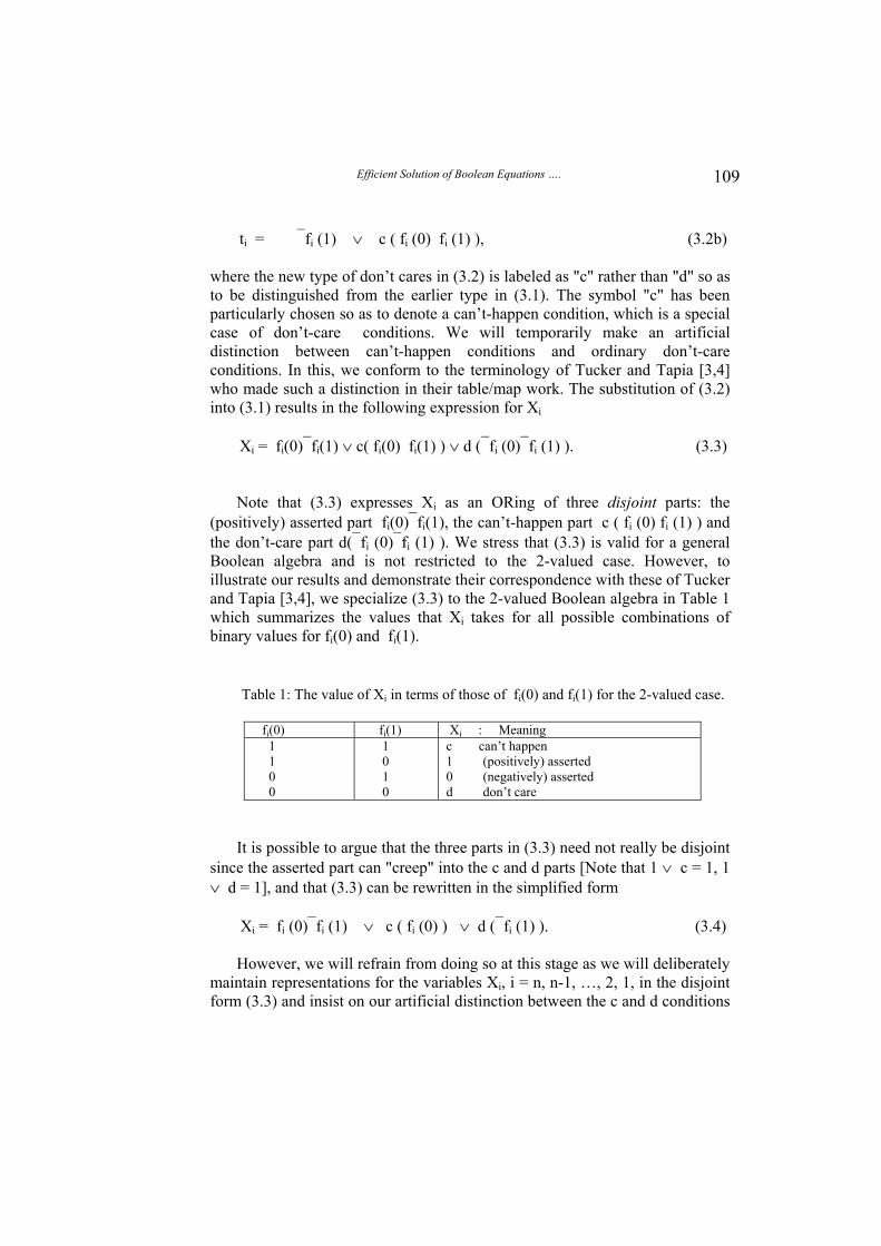
(positively) asserted part fi(0)fi(1), the can’t-happen part c ( fi (0) fi (1) ) and the don’t-care part d(fi (0)fi (1) ). We stress that (3.3) is valid for a general Boolean algebra and is not restricted to the 2-valued case. However, to illustrate our results and demonstrate their correspondence with these of Tucker and Tapia [3,4], we specialize (3.3) to the 2-valued Boolean algebra in Table 1 which summarizes the values that Xi takes for all possible combinations of binary values for fi(0) and fi(1).

Table 1: The value of Xi in terms of those of fi(0) and fi(1) for the 2-valued case.

fi(0) fi(1) Xi : Meaning 1 1 0 0

1 0 1 0

c can’t happen 1 (positively) asserted 0 (negatively) asserted d don’t care

It is possible to argue that the three parts in (3.3) need not really be disjoint

since the asserted part can "creep" into the c and d parts [Note that 1 ∨ c = 1, 1 ∨ d = 1], and that (3.3) can be rewritten in the simplified form

Xi = fi (0)fi (1) ∨ c ( fi (0) ) ∨ d (fi (1) ). (3.4) However, we will refrain from doing so at this stage as we will deliberately

maintain representations for the variables Xi, i = n, n-1, …, 2, 1, in the disjoint form (3.3) and insist on our artificial distinction between the c and d conditions


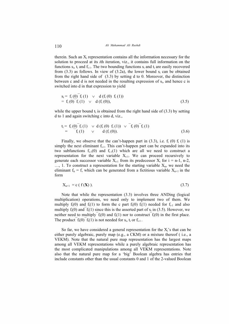
therein. Such an Xi representation contains all the information necessary for the solution to proceed at its ith iteration, viz., it contains full information on the functions si, ti and fi-1. The two bounding functions si and ti are easily recovered from (3.3) as follows. In view of (3.2a), the lower bound si can be obtained from the right hand side of (3.3) by setting d to 0. Moreover, the distinction between c and d is not needed in the resulting expression of si, and hence c is switched into d in that expression to yield

si = fi (0)fi (1) ∨ d (fi (0) fi (1)) = fi (0)fi (1) ∨ d (fi (0)), (3.5)

while the upper bound ti is obtained from the right hand side of (3.3) by setting d to 1 and again switching c into d, viz.,

ti = fi (0)fi (1) ∨ d (fi (0) fi (1)) ∨ fi (0)fi (1) = fi (1) ∨ d (fi (0)). (3.6)

Finally, we observe that the can’t-happen part in (3.3), i.e. fi (0) fi (1) is

simply the next eliminant fi-1. This can’t-happen part can be expanded into its two subfunctions fi-1(0) and fi-1(1) which are all we need to construct a representation for the next variable Xi-1. We can proceed recursively to generate each successor variable Xi-1 from its predecessor Xi for i = n-1, n-2, …, 1. To construct a representation for the starting variable Xn, we need the eliminant fn = f, which can be generated from a fictitious variable Xn+1 in the form

Xn+1 = c ( f (X) ). (3.7)

Note that while the representation (3.3) involves three ANDing (logical

multiplication) operations, we need only to implement two of them. We multiply fi(0) and fi(1) to form the c part fi(0) fi(1) needed for fi-1 and also multiply fi(0) andfi(1) since this is the asserted part of si in (3.5). However, we neither need to multiplyfi(0) and fi(1) nor to constructfi(0) in the first place. The productfi(0)fi(1) is not needed for si, ti or fi-1 .

So far, we have considered a general representation for the Xi’s that can be

either purely algebraic, purely map (e.g., a CKM) or a mixture thereof ( i.e., a VEKM). Note that the natural pure map representation has the largest maps among all VEKM representations while a purely algebraic representation has the most complicated manipulations among all VEKM representations. Note also that the natural pure map for a ‘big’ Boolean algebra has entries that include constants other than the usual constants 0 and 1 of the 2-valued Boolean


111

algebra. Such a map can be called a CKM on its pertinent algebra, but is easier to handle as a VEKM on the 2-valued Boolean algebra with the extra constants (the ones other than 1 and 0) viewed as functions of entered "variables" [1,5,7,8]. This means that while we have several choices for the 2-valued Boolean algebra, we do not have much of a choice when handling ‘big’ Boolean algebras in which case VEKMs seem to possess a clear advantage.

If the pertinent Boolean algebra is 2-valued and the Xi representation is a

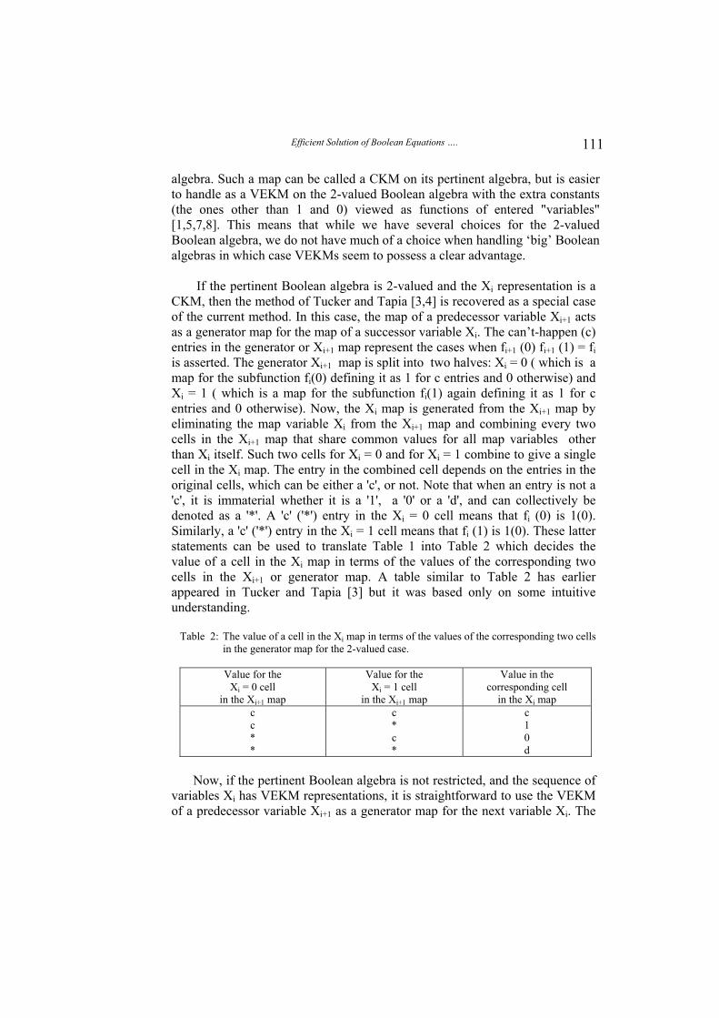
CKM, then the method of Tucker and Tapia [3,4] is recovered as a special case of the current method. In this case, the map of a predecessor variable Xi+1 acts as a generator map for the map of a successor variable Xi. The can’t-happen (c) entries in the generator or Xi+1 map represent the cases when fi+1 (0) fi+1 (1) = fi is asserted. The generator Xi+1 map is split into two halves: Xi = 0 ( which is a map for the subfunction fi(0) defining it as 1 for c entries and 0 otherwise) and Xi = 1 ( which is a map for the subfunction fi(1) again defining it as 1 for c entries and 0 otherwise). Now, the Xi map is generated from the Xi+1 map by eliminating the map variable Xi from the Xi+1 map and combining every two cells in the Xi+1 map that share common values for all map variables other than Xi itself. Such two cells for Xi = 0 and for Xi = 1 combine to give a single cell in the Xi map. The entry in the combined cell depends on the entries in the original cells, which can be either a 'c', or not. Note that when an entry is not a 'c', it is immaterial whether it is a '1', a '0' or a 'd', and can collectively be denoted as a '*'. A 'c' ('*') entry in the Xi = 0 cell means that fi (0) is 1(0). Similarly, a 'c' ('*') entry in the Xi = 1 cell means that fi (1) is 1(0). These latter statements can be used to translate Table 1 into Table 2 which decides the value of a cell in the Xi map in terms of the values of the corresponding two cells in the Xi+1 or generator map. A table similar to Table 2 has earlier appeared in Tucker and Tapia [3] but it was based only on some intuitive understanding.

Table 2: The value of a cell in the Xi map in terms of the values of the corresponding two cells

in the generator map for the 2-valued case.

Value for the Xi = 0 cell

in the Xi+1 map

Value for the Xi = 1 cell

in the Xi+1 map

Value in the corresponding cell

in the Xi map c c * *

c * c *

c 1 0 d

Now, if the pertinent Boolean algebra is not restricted, and the sequence of

variables Xi has VEKM representations, it is straightforward to use the VEKM of a predecessor variable Xi+1 as a generator map for the next variable Xi. The


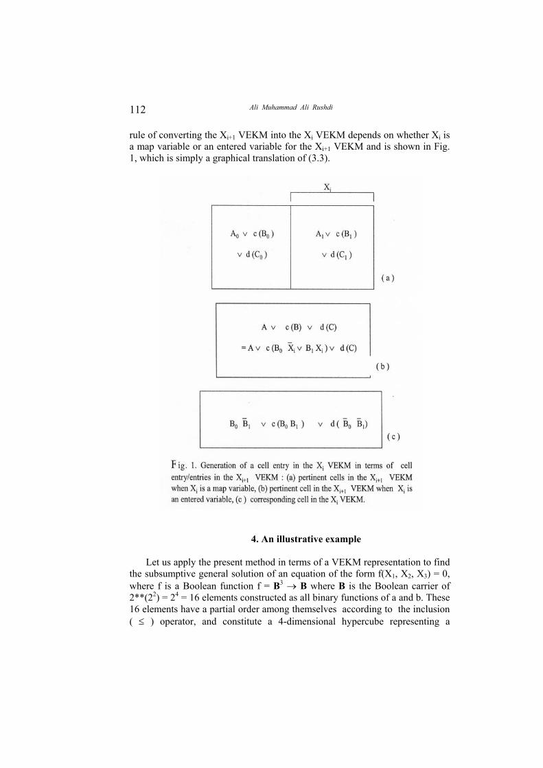
rule of converting the Xi+1 VEKM into the Xi VEKM depends on whether Xi is a map variable or an entered variable for the Xi+1 VEKM and is shown in Fig. 1, which is simply a graphical translation of (3.3).

4. An illustrative example

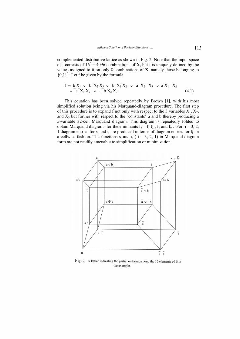
Let us apply the present method in terms of a VEKM representation to find the subsumptive general solution of an equation of the form f(X1, X2, X3) = 0, where f is a Boolean function f = B3 → B where B is the Boolean carrier of 2**(22) = 24 = 16 elements constructed as all binary functions of a and b. These 16 elements have a partial order among themselves according to the inclusion ( ≤ ) operator, and constitute a 4-dimensional hypercube representing a


113

complemented distributive lattice as shown in Fig. 2. Note that the input space of f consists of 163 = 4096 combinations of X, but f is uniquely defined by the values assigned to it on only 8 combinations of X, namely those belonging to {0,1}3 . Let f be given by the formula

f = b X1 ∨ bX2 X3 ∨ bX1 X2 ∨ aX2 X3 ∨a X1 X2

∨ aX1 X2 ∨ ab X2 X3. (4.1)

This equation has been solved repeatedly by Brown [1], with his most simplified solution being via his Marquand-diagram procedure. The first step of this procedure is to expand f not only with respect to the 3 variables X1, X2, and X3 but further with respect to the "constants" a and b thereby producing a 5-variable 32-cell Marquand diagram. This diagram is repeatedly folded to obtain Marquand diagrams for the eliminants f3 = f, f2 , f1 and f0 . For i = 3, 2, 1 diagram entries for si and ti are produced in terms of diagram entries for fi in a cellwise fashion. The functions si and ti ( i = 3, 2, 1) in Marquand-diagram form are not readily amenable to simplification or minimization.


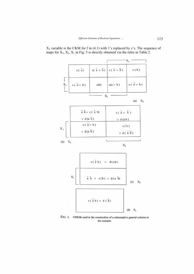
In our present procedure, however, we expand f only with respect to the true variables X1, X2, and X3 , thereby representing f by the 8-cell VEKM in Fig. 3 which has X1, X2, and X3 as map variables and has a and b as entered "variables". Since a and b are actually constants, this VEKM is a natural map for f. We switch the entries of this map into c entries and consider it a map for a fictitious variable X4 as shown in Fig. 4(a). This new map is the first in a series of generator VEKMs X4, X3, X2 and X1 given in Figs. 4(b)-4(d). The entries of a VEKM Xi, i = 3, 2, 1 are deduced from the can’t-happen entries of the predecessor or generator Xi+1 VEKM according to the transformation from (a) to (c) in Fig. 1. Now, the VEKM for every si (ti), i = 3, 2, 1, is obtained from that of the corresponding Xi with d set to 0(1) and c converted into d. The si and ti VEKMs are equivalent to those obtained for the current example by Rushdi [5], and can be used to construct minimal sum-of-products expressions via the procedure of Rushdi and Al-Yahya [8]. Finally, the subsumptive general solution for f = 0 is obtained as

a b = 0

0 ≤ X1 ≤ b a X1 ≤ X2 ≤ b ∨ X1

a X1 ≤ X3 ≤ a ∨bX2 ∨ bX2 . (4.2) The solution (4.2) is in its most simplified form, as verified from earlier

work by Brown [1], Rushdi [5], and Rudeanu [10]. For comparison purposes, Fig. 5 shows the VEKMs of Fig. 4 expanded in CKM form, with the original VEKM boundaries stressed as thick bold lines. The initial map of the fictitious


115

X4 variable is the CKM for f in (4.1) with 1’s replaced by c’s. The sequence of maps for X3, X2, X1 in Fig. 5 is directly obtained via the rules in Table 2.


117

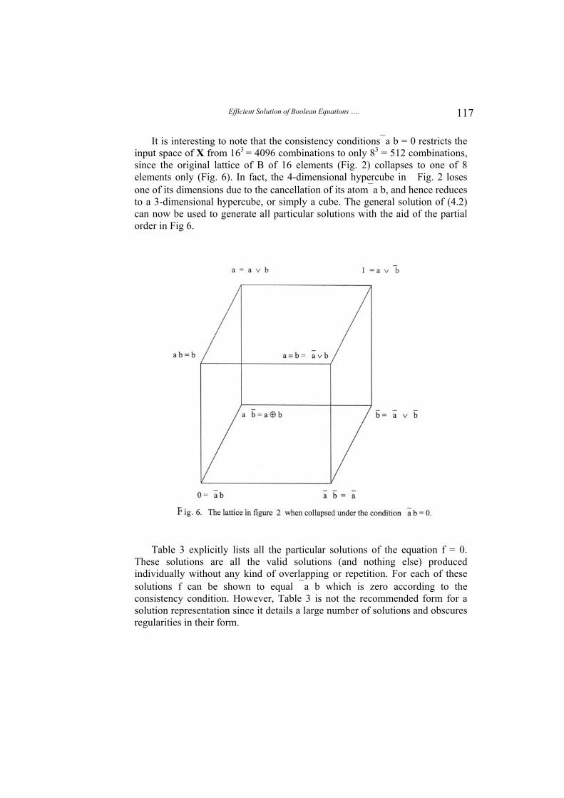
It is interesting to note that the consistency conditionsa b = 0 restricts the input space of X from 163 = 4096 combinations to only 83 = 512 combinations, since the original lattice of B of 16 elements (Fig. 2) collapses to one of 8 elements only (Fig. 6). In fact, the 4-dimensional hypercube in Fig. 2 loses one of its dimensions due to the cancellation of its atoma b, and hence reduces to a 3-dimensional hypercube, or simply a cube. The general solution of (4.2) can now be used to generate all particular solutions with the aid of the partial order in Fig 6.

Table 3 explicitly lists all the particular solutions of the equation f = 0.

These solutions are all the valid solutions (and nothing else) produced individually without any kind of overlapping or repetition. For each of these solutions f can be shown to equal a b which is zero according to the consistency condition. However, Table 3 is not the recommended form for a solution representation since it details a large number of solutions and obscures regularities in their form.


Table 3: Particular solutions equivalent to (4.2).

X1 X2 X3

X1 X2 X3

0 0 a 0 0 b 0 b a 0 b b 0 b a ∨ b 0 b 1 ab 0 a ab 0 b ab b a ab b b ab b a ∨ b ab b 1 ab ab a ab a a ab a a ∨ b a a 0 a a a a a ab a a b a a ∨ b 0 a a ∨ b a a a ∨ b ab a a ∨ b b a a ∨ b b a a ∨ b a ∨ b a a ∨ b a

a a ∨ b 1 b a 0 b a a b a ab b a b b b 0 b b a b a ∨ b 0 b a ∨ b a b a ∨ b ab b a ∨ b b b a ∨ b b b a ∨ b a ∨ b b a ∨ b a b a ∨ b 1 b 1 0 b 1 a b 1 b b 1 a ∨ b

5. Conclusions This paper presents an efficient manual method for obtaining the most

compact form of the subsumptive general solution of a system of Boolean equations. The method is an effective combination of mapping and algebraic methods (through its use of VEKM representations for Boolean functions and variables) and employs a minimum number of constructions (through its artificial distinction between don’t-care and can’t-happen conditions). Throughout its work, the method keeps track only of a single-variable representation that can have positively-asserted, don’t-care, can’t-happen or negatively-asserted components that are functions of the constants of the pertinent Boolean carrier. This single-variable representation leads to an immediate construction of the minimal sum-of-product expressions for the


119

lower and upper bound on the present variable as well as to a generation of the next variable representation. In addition to being highly economic, the present method is not restricted to two-valued Boolean equations and is naturally suitable for ‘big’ Boolean algebras.

The concepts and method developed herein can be utilized in various

application areas of Boolean equations [1,2,9,11,12]. In particular, an automated version of the present Boolean-equation solver can be applied in the simulation of gate-level logic. However, such an application must handle the incompatibility between the lattice structure of ‘big’ Boolean algebras, which are only partially ordered, and multi-valued logics, which are totally ordered [13]. The ideas expressed herein can also be incorporated in the automated solution of large systems of Boolean equations [11,14]. They can also be extended to handle quadratic Boolean equations [15], Boolean ring equations [9,16], and Boolean differential equations [17].

References

[1] Brown, F. M., Boolean Reasoning: The logic of Boolean Equations, Kluwer Academic

Publishers, Boston (1990). [2] Hammer, P. L. and S. Rudeanu, Boolean Methods in Operations Research and Related

Areas, Springer Verlag, Berlin, Germany (1968). [3] Tucker J. H., and M. A. Tapia, Using Karnaugh Maps to Solve Boolean Equations by

Successive Elimination, Proceedings of IEEE Southeastcon 92, Birmingham, AL, 2: 589-592 (1992).

[4] Tucker, J. H. and M. A. Tapia, Solution of a Class of Boolean Equations. Proceedings of IEEE Southeastcon 95, New York, NY, 1: 106-112 (1995).

[5] Rushdi, A. M., Using Variable-Entered Karnaugh Maps to Solve Boolean Equations, International Journal of Computer Mathematics, 78 (1): 23-38 (2001).

[6] Rushdi, A. M., Improved Variable-Entered Karnaugh Map Procedures, Computers and Electrical Engineering, 13 (1): 41-52 (1987).

[7] Rushdi, A. M. and H. A. Al-Yahya, A Boolean Minimization Procedure Using the Variable-Entered Karnaugh Map and the Generalized Consensus Concept, International Journal of Electronics, 87 (7): 769-794 (2000).

[8] Rushdi, A. M. and H. A. Al-Yahya, Further Improved Variable-Entered Karnaugh Map Procedures for Obtaining the Irredundant Forms of an Incompletely-Specified Switching Function, Journal of King Abdulaziz University: Engineering Sciences, 13 (1): 111-152 (2001).

[9] Rudeanu S., Boolean Functions and Equations, North-Holland Publishing Company & American Elsevier, Amsterdam, the Netherlands (1974).

[10] Rudeanu S., Algebraic Methods versus Map Methods of Solving Boolean Equations, International Journal of Computer Mathematics, 80 (7): 815-817 (2003).

[11] Crama, Y. and P. L. Hammer, Boolean Functions, E-book, Available at http://www..sig.egss.ulg.ac.be/rogp/Crama/Publications/BookPage.html, Accessed on April 15, 2002.

[12] Bochmann, D., A. D. Zakrevskij and Ch. Posthoff, Boolesche Gleichungen: Theorie, Anwendungen und Algorithmen (Boolean Equations: Theory, Applications and Algorithms) Sammelband-Verlag, Berlin, Germany (1984).


[13] Woods, S. and G. Casinovi, Multiple-Level Logic Simulation Algorithm, IEE Proceedings on Computers and Digital Techniques, 148 (3):129-137 (2001).

[14] Woods, S. and G. Casinovi, Efficient Solution of Systems of Boolean Equations, Proceedings of the 1996 IEEE/ACM International Conference on Computer-Aided Design, 542-546 (1996).

[15] Rudeanu S., On quadratic Boolean Equations, Fuzzy Sets and Systems, 75 (2): 209-213 (1995).

[16] Rudeanu S., Unique Solutions of Boolean Ring Equations, Discrete Mathematics, 122 (1-3): 381-383 (1993).

[17] Serfati, M., Boolean Differential Equations, Discrete Mathematics, 146 (1-3): 235-246 (2003).


121

الحل السريع للمعادالت البوالنية باستخدام خرائط حتوياتكارنوه متغيرة الم

علي محمد علي رشدي

قسم الهندسة الكهربائية وهندسة الحاسبات ، جامعة الملك عبد العزيز جدة ، الـمملكة العربية السعودية

يتم تقديم طريقة جديدة للحصول على حل عام :المستخلص وتعتمد الطريقة . احتوائي ملموم لنظام من المعادالت البوالنية

) خ ك غ ح (رنوه متغيرة المحتويات على استعمال خريطة كاكذلك . لتحقيق الحذف التتابعي من خالل الطي المتتابع للخريطة

ا بين اشتراطات انعدام األهمية ا مصطنًعتفتعل الطريقة تمييًزومن ثم فإنها تتمتع بكفاءة عالية . واشتراطات امتناع الحدوث

حيث إنها تتطلب إنشاء خرائط تقل في العدد بوضوح كما تصغر في الحجم بوضوح عن تلك التي تتطلبها الطرائق

عن ذلك، يمكن تطبيق الطريقة على المعادالت وفضالً. التقليديةإن تفصيالت . البوالنية العامة دون التقيد بالحالة ثنائية القيمة

الطريقة يتم تعليلها بصورة رصينة، كما يجري شرحها بعناية . ثة أمثلة توضيحيةعطى بيان لها من خالل ثالومن ثم ُي

Efficient Solution of Boolean Equations Using Variable ... · Efficient Solution of Boolean...

Documents

Transcript of Efficient Solution of Boolean Equations Using Variable ... · Efficient Solution of Boolean...