Efficient Simulations in Finance - boun.edu.tr

Efficient Simulations in Finance

Halis Sak

Department of Statistics and MathematicsWirtschaftsuniversitat Wien

Research Report Series

Report 71September 2008

http://statmath.wu-wien.ac.at/

Published online byhttp://epub.wu-wien.ac.at

EFFICIENT SIMULATIONS IN FINANCE

by

Halis Sak

B.Sc., in Mechanical Engineering, Middle East Technical University, 2000

M.Sc., in Industrial Engineering, Bogazici University, 2003

Submitted to the Institute for Graduate Studies in

Science and Engineering in partial fulfillment of

the requirements for the degree of

Doctor of Philosophy

Graduate Program in Industrial Engineering

Bogazici University

2008

ii


APPROVED BY:

Assoc. Prof. Wolfgang Hormann . . . . . . . . . . . . . . . . . . .

(Thesis Supervisor)

Assoc. Prof. Necati Aras . . . . . . . . . . . . . . . . . . .

Prof. Refik Gullu . . . . . . . . . . . . . . . . . . .

Assoc. Prof. Josef Leydold . . . . . . . . . . . . . . . . . . .

Prof. Suleyman Ozekici . . . . . . . . . . . . . . . . . . .

DATE OF APPROVAL: 30.05.2008

iii

ACKNOWLEDGEMENTS

I am grateful to my advisor, Assoc. Prof. Wolfgang Hormann for introducing me

to the field of simulation. Without his guidance and patience, I would have probably

being lost in this study. I am also grateful to the members of examining committee,

Prof. Suleyman Ozekici and Prof. Refik Gullu, for their helpful comments during my

study. It was a great pleasure for me to do my research under supervision of these

three researchers.

I had been working as a teaching assistant at Istanbul Kultur University during

most of the time of my thesis study. I want to thank Prof. Tulin Aktin for her support

as an employer during this period of time.

I have been partially supported from the scholarship program BIDEP 2211 of

The Scientific and Technological Research Council of Turkey (TUBITAK) during my

research. Many thanks to them for giving the feeling of financially secure for just doing

what we meant to do.

I have been working as a research assistant in a project for four months in the

department of Statistics and Mathematics, Vienna University of Economics and Busi-

ness Administration. I am grateful to Prof. Josef Leydold, Prof. Kurt Hornik, Karin

Haupt, Stefan Theußl and others for their support and hospitality during my time in

Vienna.

I want to thank my brothers, parents and to all who really care about me. Finally,

I want to specifically thank Hasim Sak and Sibel Tombaz for their support and love.

iv

ABSTRACT


Measuring the risk of a credit portfolio is a challenge for financial institutions

because of the regulations brought by the Basel Committee. In recent years lots of

models and state-of-the-art methods, which utilize Monte Carlo simulation, were pro-

posed to solve this problem. In most of the models factors are used to account for the

correlations between obligors. We concentrate on the the normal copula model, which

assumes multivariate normality of the factors. Computation of value at risk (VaR) and

expected shortfall (ES) for realistic credit portfolio models is subtle, since, (i) there is

dependency throughout the portfolio; (ii) an efficient method is required to compute

tail loss probabilities and conditional expectations at multiple points simultaneously.

This is why Monte Carlo simulation must be improved by variance reduction tech-

niques such as importance sampling (IS). Optimal IS probabilities are computed and

compared with the “asymptotically optimal” probabilities for credit portfolios consist-

ing of groups of independent obligors. Then, a new method is developed for simulating

tail loss probabilities and conditional expectations for a standard credit risk portfolio.

The new method is an integration of IS with inner replications using geometric short-

cut for dependent obligors in a normal copula framework. Numerical results show that

the new method is better than naive simulation for computing tail loss probabilities

and conditional expectations at a single x and VaR value. Furthermore, it is clearly

better than two-step IS in a single simulation to compute tail loss probabilities and

conditional expectations at multiple x and VaR values. Then, the performance of outer

IS strategies, which consider only shifting the mean of the systematic risk factors of

realistic credit risk portfolios are evaluated. Finally, it is shown that compared to the

standard t statistic a skewness-correction method of Peter Hall is a simple and more

accurate alternative for constructing confidence intervals.

v

OZET

VERIMLI FINANSAL SIMULASYONLAR

Basel komitesinin duzenlemeleri finansal enstituler icin zor bir is olan kredi

portfoy riskinin hesaplanmasını zorunlu kılar. Son yıllarda bir cok model ve Monte

Carlo simulasyonunu kullanan metodlar gelistirilmistir. Bu modellerin cogunda yukumluler

arası korrelasyonu saglamak icin faktorler kullanılır. Biz cok-faktorlu normalligin kabul

edildigi normal kapula modeli uzerinde yogunlasırız. Gercekci kredi potfoy modelleri

icin riskteki deger (VaR) ve beklenen kuyruk kaybı (ES) hesaplanması kompleks bir

istir, cunku; (i) portfoy icinde bagımlılık vardır; (ii) kuyruk kayıp olasılıklarını ve sartlı

beklentileri coklu noktalarda aynı anda verebilecek verimli bir metoda gereksinim duyu-

lur. Bu yuzden Monte Carlo simulasyonu onemli ornekleme (IS) gibi varyasyon azaltma

teknikleri ile gelistirilmelidir. Bagımsız ve kucuk guruplara bolunebilen yukumlulerden

olusan kredi portfoyleri icin en iyi IS olasılıkları hesaplanır ve bunlar “en iyi asim-

totik” olasılıklarla karsılastırılır. Daha sonra standart kredi portfoyleri icin kuyruk

kayıp olasılıklarını ve sartlı beklentileri simule edecek yeni bir metod gelistirilir. Yeni

metod normal kopula kapsamındaki bagımlı yukumluler icin IS’in geometrik kısa yolu

kullananan icsel replikasyonlarla birlesimidir. Numeriksel sonuclar, yeni metodun tek

bir x ve VaR degeri icin standart simulasyondan daha iyi oldugunu ortaya koyar.

Buna ek olarak, tek bir simulasyonda birden fazla x ve VaR degerleri icin kuyruk

kayıp olasılıklarının ve sartlı beklentilerinin hesaplanmasında iki-asamalı IS’den acık bir

sekilde daha iyidir. Daha sonra, gercekci kredi portfoyleri uzerinde sadece sistematik

risk faktorlerinin ortalamasını arttıran dıssal IS stratejileri incelenir. En sonunda, stan-

dart t istatistigiyle karsılastırıldıgında Peter Hall’un yamukluk duzeltme metodunun

guven aralıgı olusturulmasında kolay ve daha kesin bir alternatif oldugu gosterilir.

vi

TABLE OF CONTENTS

ACKNOWLEDGEMENTS . . . . . . . . . . . . . . . . . . . . . . . . . . . . . iii

ABSTRACT . . . . . . . . . . . . . . . . . . . . . . . . . . . . . . . . . . . . . iv

OZET . . . . . . . . . . . . . . . . . . . . . . . . . . . . . . . . . . . . . . . . . v

LIST OF FIGURES . . . . . . . . . . . . . . . . . . . . . . . . . . . . . . . . . viii

LIST OF TABLES . . . . . . . . . . . . . . . . . . . . . . . . . . . . . . . . . . xiii

LIST OF SYMBOLS/ABBREVIATIONS . . . . . . . . . . . . . . . . . . . . . xix

1. INTRODUCTION . . . . . . . . . . . . . . . . . . . . . . . . . . . . . . . . 1

2. THE CREDIT RISK MODEL . . . . . . . . . . . . . . . . . . . . . . . . . . 6

2.1. The Normal Copula Model . . . . . . . . . . . . . . . . . . . . . . . . . 6

2.2. Simulation . . . . . . . . . . . . . . . . . . . . . . . . . . . . . . . . . . 7

2.2.1. Naive Monte Carlo Simulation . . . . . . . . . . . . . . . . . . . 7

2.2.2. Importance Sampling . . . . . . . . . . . . . . . . . . . . . . . . 8

2.2.3. The Algorithm of Glasserman & Li . . . . . . . . . . . . . . . . 9

3. OPTIMAL IS FOR INDEPENDENT OBLIGORS . . . . . . . . . . . . . . . 14

3.1. Exponential Twisting for Binomial Distribution . . . . . . . . . . . . . 14

3.2. Optimal IS Probabilities . . . . . . . . . . . . . . . . . . . . . . . . . . 16

3.2.1. One Obligor Case . . . . . . . . . . . . . . . . . . . . . . . . . 16

3.2.2. Two Obligors Case . . . . . . . . . . . . . . . . . . . . . . . . . 20

3.2.3. One Homogeneous Group of Obligors . . . . . . . . . . . . . . . 29

3.2.4. Two Homogenous Groups of Obligors . . . . . . . . . . . . . . . 33

3.3. Application Example . . . . . . . . . . . . . . . . . . . . . . . . . . . . 46

3.3.1. Example 2 . . . . . . . . . . . . . . . . . . . . . . . . . . . . . . 50

4. A NEW ALGORITHM FOR THE NORMAL COPULA MODEL . . . . . . 52

4.1. Geometric Shortcut: Independent Obligors . . . . . . . . . . . . . . . . 52

4.2. Inner Replications using Geometric Shortcut: Dependent Obligors . . . 54

4.3. Integrating IS with Inner Replications using the Geometric Shortcut:

Dependent Obligors . . . . . . . . . . . . . . . . . . . . . . . . . . . . . 58

4.4. Computing Conditional Expectation of Loss: Dependent Obligors . . . 60

4.5. Numerical Results . . . . . . . . . . . . . . . . . . . . . . . . . . . . . 62

vii

4.5.1. Simultaneous Simulations . . . . . . . . . . . . . . . . . . . . . 67

4.6. Conclusion . . . . . . . . . . . . . . . . . . . . . . . . . . . . . . . . . . 72

5. COMPARISON OF MEAN SHIFTS FOR IS . . . . . . . . . . . . . . . . . . 73

5.1. Mode of Zero-Variance IS Distribution . . . . . . . . . . . . . . . . . . 73

5.1.1. Tail Bound Approximation . . . . . . . . . . . . . . . . . . . . . 74

5.1.2. Normal Approximation . . . . . . . . . . . . . . . . . . . . . . . 75

5.2. Homogenous Portfolio Approximation . . . . . . . . . . . . . . . . . . . 75

5.3. Numerical Results . . . . . . . . . . . . . . . . . . . . . . . . . . . . . 77

6. BETTER CONFIDENCE INTERVALS FOR IS . . . . . . . . . . . . . . . . 83

6.1. Hall’s Transformation of the t Statistic . . . . . . . . . . . . . . . . . . 83

6.2. TWO EXAMPLES . . . . . . . . . . . . . . . . . . . . . . . . . . . . . 84

6.2.1. Example 1 . . . . . . . . . . . . . . . . . . . . . . . . . . . . . . 84

6.2.2. Example 2 . . . . . . . . . . . . . . . . . . . . . . . . . . . . . . 85

6.3. Credit Risk Application . . . . . . . . . . . . . . . . . . . . . . . . . . 88

7. CONCLUSIONS . . . . . . . . . . . . . . . . . . . . . . . . . . . . . . . . . 92

APPENDIX A: ADDITIONAL NUMERICAL RESULTS AND NOTES . . . 94

A.1. Additional Numerical Results For Chapter 3 . . . . . . . . . . . . . . . 94

A.2. Asymptotically Optimal Mean Shift For One Dimensional Portfolio

Problem . . . . . . . . . . . . . . . . . . . . . . . . . . . . . . . . . . . 98

APPENDIX B: C CODES . . . . . . . . . . . . . . . . . . . . . . . . . . . . . 99

B.1. Common Codes . . . . . . . . . . . . . . . . . . . . . . . . . . . . . . . 99

B.2. Codes For The New Algorithm For The Normal Copula Model . . . . . 104

B.3. Codes For The Comparison of Mean Shifts For IS . . . . . . . . . . . . 120

B.4. Codes For The Better Confidence Intervals For IS . . . . . . . . . . . . 128

REFERENCES . . . . . . . . . . . . . . . . . . . . . . . . . . . . . . . . . . . . 132

REFERENCES NOT CITED . . . . . . . . . . . . . . . . . . . . . . . . . . . . 136

viii

LIST OF FIGURES

Figure 2.1. Tail loss probability computation using exponential twisting for

independent obligors. . . . . . . . . . . . . . . . . . . . . . . . . . 11

Figure 2.2. Tail loss probability computation using two-step IS of [13] for de-

pendent obligors. . . . . . . . . . . . . . . . . . . . . . . . . . . . 13

Figure 3.1. Naive simulation algorithm for P (L > x) (one obligor case) . . . . 17

Figure 3.2. IS algorithm for P (L > x) (one obligor case) . . . . . . . . . . . . 17

Figure 3.3. Naive simulation algorithm for E[L|L > x] (one obligor case) . . . 19

Figure 3.4. IS algorithm for E[L|L > x] (one obligor case) . . . . . . . . . . . 19

Figure 3.5. Naive simulation algorithm for P (L > x) (two independent obligors

case) . . . . . . . . . . . . . . . . . . . . . . . . . . . . . . . . . . 21

Figure 3.6. IS algorithm for P (L > x) (two independent obligors case) . . . . 21

Figure 3.7. Naive simulation algorithm for E[L|L > x] (two independent oblig-

ors case) . . . . . . . . . . . . . . . . . . . . . . . . . . . . . . . . 25

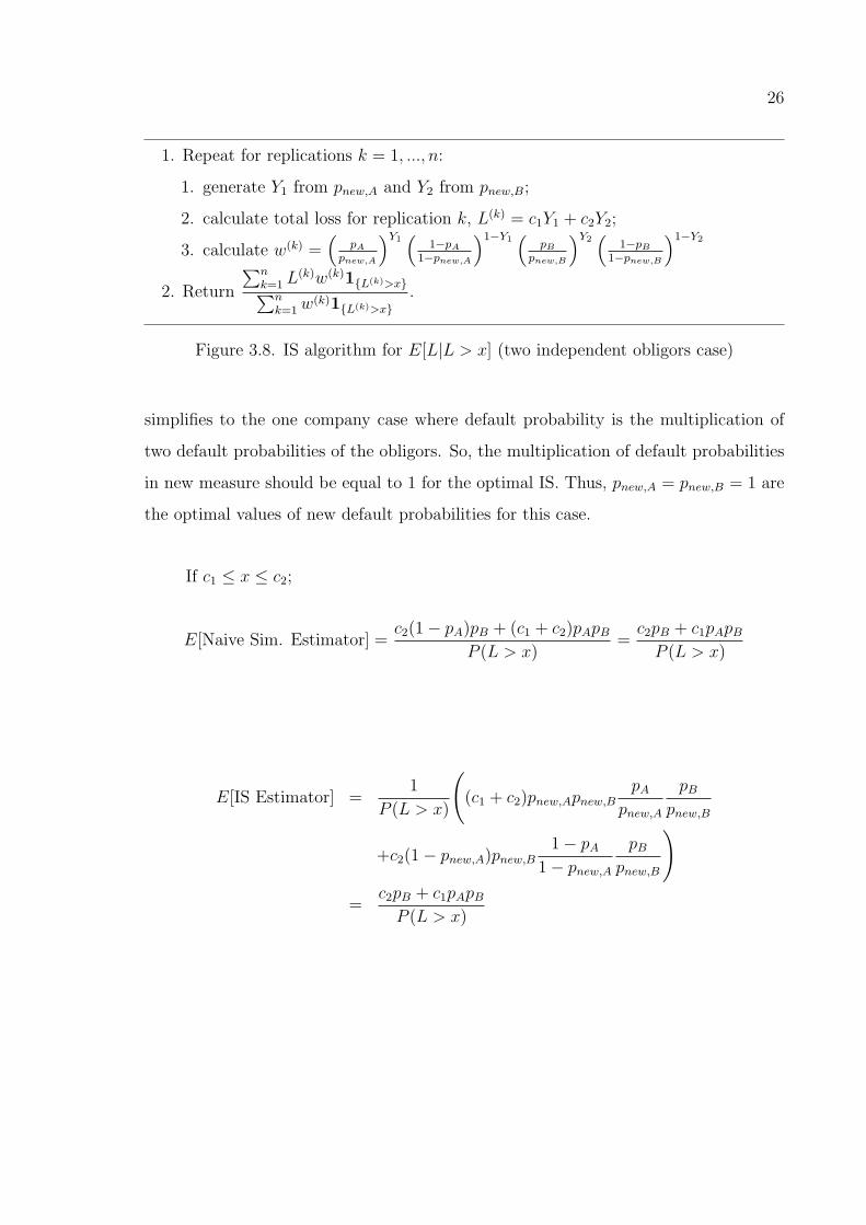
Figure 3.8. IS algorithm for E[L|L > x] (two independent obligors case) . . . 26

Figure 3.9. Naive simulation algorithm for P (L > x) (One homogeneous group

of obligors case) . . . . . . . . . . . . . . . . . . . . . . . . . . . . 29

Figure 3.10. IS algorithm for P (L > x) (One homogeneous group of obligors case) 30

ix

Figure 3.11. Naive simulation algorithm for E[L|L > x] (One homogeneous

group of obligors case) . . . . . . . . . . . . . . . . . . . . . . . . 31

Figure 3.12. IS algorithm for E[L|L > x] (One homogeneous group of obligors

case) . . . . . . . . . . . . . . . . . . . . . . . . . . . . . . . . . . 32

Figure 3.13. Naive simulation algorithm for P (L > x) (Two homogeneous groups

of obligors case) . . . . . . . . . . . . . . . . . . . . . . . . . . . . 34

Figure 3.14. IS algorithm for P (L > x) (Two homogeneous groups of obligors

case) . . . . . . . . . . . . . . . . . . . . . . . . . . . . . . . . . . 34

Figure 3.15. Optimal and exponential twisting [13] probabilities and correspond-

ing variances for pA = 0.05, pB = 0.05,mA = 5,mB = 2 and x = 2

in computing P (L > x). . . . . . . . . . . . . . . . . . . . . . . . . 36



in computing P (L > x). . . . . . . . . . . . . . . . . . . . . . . . . 37



in computing P (L > x). . . . . . . . . . . . . . . . . . . . . . . . . 37



in computing P (L > x). . . . . . . . . . . . . . . . . . . . . . . . . 38


ing variances for pA = 0.05, pB = 0.05,mA = 100,mB = 50 and

x = 30 in computing P (L > x). . . . . . . . . . . . . . . . . . . . 38

x



x = 30 in computing P (L > x). . . . . . . . . . . . . . . . . . . . 39

Figure 3.21. Naive simulation algorithm for E[L|L > x] (Two homogeneous

group of obligors case) . . . . . . . . . . . . . . . . . . . . . . . . 40

Figure 3.22. IS algorithm for E[L|L > x] (Two homogeneous group of obligors

case) . . . . . . . . . . . . . . . . . . . . . . . . . . . . . . . . . . 40



in computing E[L|L > x]. . . . . . . . . . . . . . . . . . . . . . . . 42












x = 30 in computing E[L|L > x]. . . . . . . . . . . . . . . . . . . 44

xi



x = 30 in computing E[L|L > x]. . . . . . . . . . . . . . . . . . . 45

Figure 4.1. Tail loss probability computation using naive simulation for inde-

pendent obligors. . . . . . . . . . . . . . . . . . . . . . . . . . . . 52

Figure 4.2. Geometric shortcut in generating default indicators . . . . . . . . 53

Figure 4.3. Tail loss probability simulation using the geometric shortcut for

independent obligors. . . . . . . . . . . . . . . . . . . . . . . . . . 54

Figure 4.4. Tail loss probability computation using naive simulation for depen-

dent obligors. . . . . . . . . . . . . . . . . . . . . . . . . . . . . . 55

Figure 4.5. Inner replications using geometric shortcut in generating default

indicators . . . . . . . . . . . . . . . . . . . . . . . . . . . . . . . 56

Figure 4.6. Tail loss probability simulation using inner replications using the

geometric shortcut for dependent obligors. . . . . . . . . . . . . . 57

Figure 4.7. Tail loss probability simulation using integration of IS with inner

replications using the geometric shortcut for dependent obligors. . 59

Figure 4.8. Naive simulation for computing ES for dependent obligors. . . . . 60

Figure 4.9. ES simulation using integration of IS with inner replications using

the geometric shortcut for dependent obligors. . . . . . . . . . . . 62

Figure 4.10. Comparison of new method with IS in estimating tail loss proba-

bilities in the 10-factor model using 1, 000 replications. . . . . . . 70

xii

Figure 4.11. Comparison of new method with IS in estimating expected shortfall

in the 10-factor model using 10, 000 replications. . . . . . . . . . . 71

xiii

LIST OF TABLES

Table 3.1. Portfolio composition (one obligor case) . . . . . . . . . . . . . . . 16

Table 3.2. Loss Distribution for the portflio (one obligor case) . . . . . . . . . 17

Table 3.3. Portfolio composition (independent two obligors) . . . . . . . . . . 20

Table 3.4. Loss Distribution for the portio (independent two obligors) . . . . 20

Table 3.5. Optimal (OP) and exponential twisting probabilities (ETP) and

corresponding standard deviations (sd) to compute P (L > x) (Two

independent obligors case). . . . . . . . . . . . . . . . . . . . . . . 25

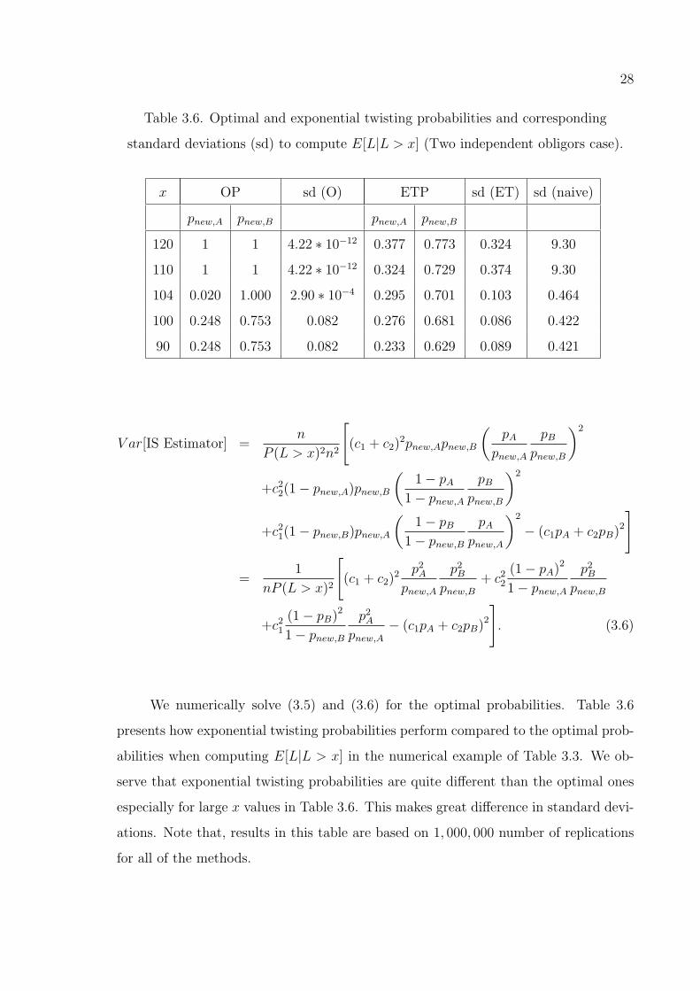
Table 3.6. Optimal and exponential twisting probabilities and corresponding

standard deviations (sd) to compute E[L|L > x] (Two independent

obligors case). . . . . . . . . . . . . . . . . . . . . . . . . . . . . . 28

Table 3.7. Optimal and exponential twisting IS probabilities and correspond-

ing standard deviations (sd) for the parameter values of m = 100

and p = 0.1 to compute P (L > x). . . . . . . . . . . . . . . . . . . 31


ing standard deviations (sd) for the parameter values of m = 100

and p = 0.1 to compute E[L|L > x]. . . . . . . . . . . . . . . . . . 33


variances (var). . . . . . . . . . . . . . . . . . . . . . . . . . . . . . 36


ing variances (var). . . . . . . . . . . . . . . . . . . . . . . . . . . 42

xiv

Table 3.11. Profiles of bonds included in the mutual funds . . . . . . . . . . . 47


ing variances to compute P (W < x). . . . . . . . . . . . . . . . . . 48


ing variances to compute E[W |W < x]. . . . . . . . . . . . . . . . 49

Table 3.14. Variances for simulating P (L > x) under IS using optimal and

exponential twisting probabilities and naive simulation. . . . . . . 51

Table 3.15. Variances for simulating E[L|L > x] under IS using optimal and

exponential twisting probabilities and naive simulation. . . . . . . 51

Table 4.1. Tail loss probabilities and half lengths (hl) of the confidence in-

tervals for naive, IS and the new method in the 10-factor model.

n = 10, 000. Execution times (in seconds) are in parentheses. . . . 64

Table 4.2. ES values and half lengths (hl) of the confidence intervals using

naive, IS and the new method in the 10-factor model. n = 100, 000.

Execution times (in seconds) are in parentheses. . . . . . . . . . . 64







Table 4.5. Portfolio composition for the 5-factor model; default probabilities,

exposure levels and factor loadings for six segments. . . . . . . . . 66

xv







Table 4.8. Tail loss probabilities and half lengths (hl) of the confidence inter-

vals in a single simulation using naive, IS and the new method in

the 10-factor model. n = 10, 000. Execution times for the methods

are 7, 16 and 12 seconds in the given order. . . . . . . . . . . . . . 69

Table 4.9. ES values and half lengths (hl) of the confidence intervals in a single

simulation using naive, IS and the new method in the 10-factor

model. n = 100, 000. Execution times for the methods are 66, 151

and 104 seconds in the given order. . . . . . . . . . . . . . . . . . . 69

Table 5.1. Half lengths (hl) of the confidence intervals for using tail bound ap-

proximation (TBA), normal approximation (NA) and homogenous

approximation (HA) for the optimal mean shift as outer IS and ex-

ponential twisting as inner IS in the 10-factor model to compute

tail loss probabilities. n = 10, 000. Execution times (in seconds)

are in parentheses. . . . . . . . . . . . . . . . . . . . . . . . . . . . 78





expected shortfalls. n = 100, 000. Execution times (in seconds) are

in parentheses. . . . . . . . . . . . . . . . . . . . . . . . . . . . . . 79

xvi





tail loss probabilities. n = 10, 000. Execution times (in seconds)

are in parentheses. . . . . . . . . . . . . . . . . . . . . . . . . . . . 80






in parentheses. . . . . . . . . . . . . . . . . . . . . . . . . . . . . . 80




ponential twisting as inner IS in the 5-factor model to compute tail

loss probabilities. n = 10, 000. Execution times (in seconds) are in

parentheses. . . . . . . . . . . . . . . . . . . . . . . . . . . . . . . 81



approximation (HA) for the optimal mean shift as outer IS and

exponential twisting as inner IS in the 5-factor model to compute


in parentheses. . . . . . . . . . . . . . . . . . . . . . . . . . . . . . 81

Table 6.1. Achieved coverage levels for 95 percent upper and lower endpoint

confidence intervals (x = 2) . . . . . . . . . . . . . . . . . . . . . . 86

xvii


confidence intervals (S0 = 100, r = 0.09). . . . . . . . . . . . . . . 87

Table 6.3. Nearly exact tail loss probabilities and upper and lower bound of

the confidence intervals by using ordinary t statistics and Hall’s

method in the 10-factor model. n = 1, 000. . . . . . . . . . . . . . 88



method in the 21-factor model. n = 1, 000. . . . . . . . . . . . . . 89



method in the 5-factor model. n = 1, 000. . . . . . . . . . . . . . . 89


confidence intervals for computing tail loss probabilities. n = 1, 000. 90

Table A.1. Optimal and exponential twisting [13] probabilities and percent dif-

ferences of variances between exponential twisting and optimal (%

diff. of var. ET-O) and naive simulation and optimal (percent diff.

of var. naive-O) for x = 1 in computing P (L > x). . . . . . . . . . 94



diff. of var. ET-O) and naive simulation and optimal (% diff. of

var. naive-O) for x = 1 in computing E[L|L > x]. . . . . . . . . . . 95



diff. of var. ET-O) and naive simulation and optimal (% diff. of

var. naive-O) for x = 5 in computing P (L > x). . . . . . . . . . . 96

xviii

Table A.4. Optimal and Exponential Twisting ( [13]) probabilities and percent

differences of variances between exponential twisting and optimal

(% diff. of var. ET-O) and naive simulation and optimal (% diff.

of var. naive-O) for x = 5 in computing E[L|L > x]. . . . . . . . . 97

Table A.5. Optimal mean shifts for various x values. . . . . . . . . . . . . . . 98

xix

LIST OF SYMBOLS/ABBREVIATIONS

ajl Factor loading of jth obligor for risk factor l

A First group of obligors

B Second group of obligors

c Loss resulting from default of an obligor or homogenous loss

cA Loss resulting from default of an obligor in group A

cB Loss resulting from default of an obligor in group B

cj Loss resulting from default of jth obligor

c∞ 100(1− α)% quantile of L∞d

Cov(Zk, Zl) Covariance between Zk and Zl

d Number of systematic risk factors

gj Weight for obligor j

E[T ] Expectation of a random variable T

E[T |S] Expectation of a random variable T conditional on an event

S

Eθ Expectation under exponential twisting with parameter θ

erfc(z) Complementary error function of z

exp(z) Exponential function of z

I Identity matrix

L Total loss of portfolio

Li ith possible (having probability greater than zero) loss value

in the portfolio loss distribution

L∞d Infinite homogenous portfolio loss function

L(k) Total loss of portfolio for replication k

m Number of obligors in portfolio

mA Number of obligors in group A

mB Number of obligors in group B

M2(x, θ) Second moment of estimator for P (L > x) for exponential

twisting with parameter θ

n Number of replications

xx

nin Number of inner replications

Nµ,σ Normal density function with mean µ and variance σ

p Default probability of an obligor or homogenous default prob-

ability

P Probability measure

pA Default probability of an obligor in group A

pB Default probability of an obligor in group B

pj Marginal default probability of jth obligor

pnew IS default probability

pnew,A IS default probability for obligors in group A

pnew,B IS default probability for obligors in group B

P (S) Probability of an event S

pZ Average of the conditional default probabilities for obligors

Q Importance Sampling probability measure

rs Speed up ratio

s Scaling factor to normalize weighted sum of factor loadings

V ar[T ] Variance of a random variable T

w Likelihood ratio

w(k) Likelihood ratio for replication k

X Multivariate normal vector of latent variables

Y Default indicator for an obligor (1 if default, 0 otherwise)

Yj Default indicator for jth obligor (1 if default, 0 otherwise)

Z Multivariate standard normal random variable for systematic

risk factors

Zl Standard normal random variable for systematic risk factor l

zδ/2 (1− δ/2) percentile of the standard normal distribution

1− α Probability level at which confidence interval is given

εj Idiosyncratic risk factor for obligor j

θ Exponential twisting parameter

µ Mean shift vector in IS

φ Density function for P

xxi

ψ Density function for Q

ψL(θ) Cumulant generating function of L given θ

Φ Standard normal cumulative distribution function

Ψ Weighted sum of factor loadings

CI Confidence Interval

ES Expected Shortfall

ET Exponential twisting

ETP Exponential twisting probability

GSL GNU Scientific Library

HA Homogenous approximation

hl Half length of confidence interval

IS Importance Sampling

max Maximize

NA Normal approximation

O Optimal IS

OP Optimal IS probability

prob. Probability

skw Skewness

sd Standard deviation

sup Supremum (least upper bound)

TBA Tail bound approximation

var Variance

VaR Value at Risk

VaRα Value at Risk at 100(1− α) percent confidence level

VR Variance Ratio

1

1. INTRODUCTION

Financial institutions are subject to a wide range of risks. [6] classifies them as

market risk, credit risk, liquidity risk, operational risk and systematic risk. This thesis

study considers only credit risk, which can be defined as risks associated with default

of obligors to make payments or changes in their credit quality.

Measuring the credit portfolio risk is a challenge for financial institutions because

of the regulations brought by Basel Committee [3]. In recent years lots of models

(see [4]) and state-of-the-art methods, which utilize Monte Carlo simulation, (see [11])

were proposed to solve this problem. The proposed models are with the exception of

CreditPortfolio View [27] factor based models. They use factors to account for the

correlations in the defaults of obligors. This ease the calibration of the models and

decrease computational effort for correlated losses. However, [20] report that multi-

factor models should be adjusted to achieve Basel II-consistent results and they show

how to do that.

We concentrate on the the normal copula model of [19], a Merton [29] type model,

to capture the dependence across obligors. Underlying risk factors are assumed to be

normal in this model. However, we are aware of the risks of using this model because

of weak tail dependence (see [8]).

Value at Risk (VaR) has been quite popular as a risk measure to be used in credit

risk models because of being conceptually simple and easy-to-compute. It is simply the

quantile of portfolio loss distribution. [2] defines VaR at 100(1−α) percent confidence

level (VaRα(X)) as

VaRα(X) = sup{x|P [X ≥ x] > α}

where sup{x|A} is the upper limit of x given event A.

2

Nevertheless, there are some shortcomings of VaR (see [1] and [2]). To summarize,

it ignores losses beyond VaR and is not coherent. [1] proposes Expected Shortfall (ES)

to solve the problems of VaR. ES is simply the expected amount of losses that are

larger than the VaR level. Thus, ES is defined as:

ESα(X) = E[X|X ≥ VaRα(X)]

for the 100(1− α) percent confidence level.

Computation of VaR and ES for realistic portfolio models is subtle, since, (i) there

is dependency throughout the portfolio; (ii) an efficient method is required to compute

tail loss probabilities and conditional expectations at multiple points simultaneously.

This is why Monte Carlo simulation is a widely used tool here. But, simulation is

not an easy option either. We need to apply variance reduction techniques such as IS,

control variate, etc. (see [11], Chapter 4) for rare-event simulations, simulating tail

loss probabilities and conditional expectations.

Variance reduction techniques for simulating tail loss probabilities and conditional

expectations in the normal copula framework are “hot topics”. Previous studies in

importance sampling (IS), in the the normal copula model, can be summarized as:

(a) outer IS: applying IS to common factors (see [7, 25]);

(b) inner IS: applying IS on the resulting conditional default probabilities (see [28]);

(c) two-step IS: applying outer IS first, then inner IS (see [12, 13,18]).

These papers apply different but similar methodologies to slightly different problems.

Note that all these works were finished in the last 4 years.

[13] and [28] apply an importance sampling (IS) technique which utilizes expo-

nentially twisted Bernoulli mass functions discussed in [31] for computing P (L > x).

Furthermore, [18] applies IS approach of [13], to the integrated market and credit

portfolio model described in [17].

3

[13] and [28] not only apply exponential twisting, but also show that it is “asymp-

totically optimal”1 for loss exceedance probabilities. However, [15] shows that asymp-

totically optimality of IS based on exponential twisting is true only in one point.

Moreover, [7] report that for practical purposes, asymptotically optimal IS methods

may fail. Even, they may perform worse than naive simulation for a typical medium-

sized portfolio. And, they propose an IS approach that is based on adaptive stochastic

approximation of Robbins-Monro.

It is well known that whenever we have a large skewness in a simulation, standard

method of using t statistc for the confidence interval construction for the mean does not

give robust results (see [11]). However, there are studies on how to decrease the effect

of skewness of the population when doing tests on the mean such as confidence interval

construction and hypothesis testing. [23] propose a transformation (Johnson’s trans-

formation) on the t variable to correct for the bias on the mean, but [21] reports that

it fails to correct for skewness. [21] propose another transformation (Hall’s transforma-

tion) that has desirable characteristics of monotonicity and invertibility to correct for

both bias and skewness from the distribution of t statistic. Furthermore, [34] compares

the performance of Johnson’s and Hall’s transformations and their bootstrap versions

by looking at the coverage accuracy of one-sided confidence intervals.

The organization of the thesis is as follows.

In Chapter 2 we first describe the widely used dependency model across obligors in

a credit portfolio called here the normal copula model (see Section 2.1). In that section

we also introduce the notation, which will be used throughout the thesis. In Section

2.2 we talk about simulation and one of the classical variance reduction techniques, IS.

Finally, we describe the IS approach of [13] for the normal copula model.

In Chapter 3 we show how to compute the optimal importance sampling proba-

bilities for credit portfolios consisting of groups of independent obligors both for tail

1asymptotically optimality refers to the case where the second moment decreases at the fastestpossible rate among all unbiased estimators as the event becomes rare (see [13]).

4

loss probability and expected shortfall simulation. In Section 3.1 we show that we

can apply exponential twisting directly on the binomial distribution to simulate tail

loss probabilities. In Section 3.2 we compare the optimal IS probabilities with the

“asymptotically optimal” ones for groups of obligors. In Section 3.3 we show how our

methodology which is used throughout the chapter can be used to compute optimal

probabilities for two small financial examples.

In Chapter 4 we propose a new efficient simulation method for computing tail

loss probabilities and conditional expectations in the normal copula framework. We

replace inner IS by inner replications implemented by a geometric shortcut in the two-

step IS of [13]. Section 4.1 analyzes the geometric shortcut for independent obligors.

In section 4.2 we consider dependent obligors and introduce the geometric shortcut

for inner replications. In Section 4.3 we add outer-IS to the inner replications of the

geometric shortcut for a portfolio having dependent obligors. While Sections 4.1-4.3

concentrate on the efficient simulations for computing tail loss probabilities, Section 4.4

applies our new method to the simulation of conditional expectations. We summarize

our numerical results in Section 4.5. Finally, we conclude in Section 4.6.

In Chapter 5 we evaluate outer IS strategies, which consider only shifting the

mean of the systematic risk factors in the numerical examples of Chapter 4. In Section

5.1 we describe the tail bound approximation used in [13] and the normal approxi-

mation used in Chapter 4, which are then used to find the mode of the zero-variance

IS distribution. In Section 5.2 we describe the homogenous portfolio approximation

of [25]. In Section 5.3 we assess the performance of these three ways to calculate the

mean shifts for the numerical examples of Chapter 4.

In Chapter 6 we evaluate the performance of Hall’s transformation in correcting

the confidence intervals for financial simulations that include IS. In Section 6.1 we give

the details of Hall’s transformation. In Section 6.2.1 and 6.2.2 we describe a portfolio

risk and an option pricing example and compare the coverage accuracy of one-sided

confidence intervals using ordinary t statistic and Hall’s transformation. For both of

the problems we have analytical solutions. In Section 6.3 we compare the performance

5

of Hall’s condence intervals and standard t intervals for the numerical examples of

Chapter 4.

We conclude in Chapter 7.

6

2. THE CREDIT RISK MODEL

2.1. The Normal Copula Model

We are interested in the the normal copula model of CreditMetrics (see [19])

for the dependence structure across obligors. We first of all give the notation used

throughout the thesis which is similar to [13].

m: number of obligors in portfolio

Yj: default indicator for jth obligor (equal to 1 if default occurs, 0 otherwise)

cj: loss resulting from the default of jth obligor

pj: marginal default probability of jth obligor

L =∑m

j=1 cjYj: total loss of portfolio

n: number of replications in a simulation

Our aim is to assess the distribution of tail loss probability and ES over a fixed

horizon. Values of cj’s are known and constant over the fixed horizon. Furthermore,

we assume that the marginal default probabilities (pj’s) are known.

The normal copula model introduces a multivariate normal vector (X1, ..., Xm) of

latent variables to obtain dependence across obligors. Relationship between the default

indicators and the latent variables are represented by

Yj = 1{Xj>xj}, j = 1, ...,m,

where Xj has standard normal distribution and xj = Φ−1(1− pj), with Φ−1 inverse of

the standard normal cumulative distribution function. Obviously, the threshold value

of xj is chosen such that P (Yj = 1) = pj.

The correlations among Xj are modeled as

Xj = bjεj + aj1Z1 + ...+ ajdZd, j = 1, ...,m, (2.1)

7

where εj and Z1, ..., Zd are independent standard normal random variables with b2j +

a2j1+...+a2

jd = 1. While, (Z1, ..., Zd) are systematic risk factors affecting all of the oblig-

ors, εj is the idiosyncratic risk factor affecting only obligor j. Furthermore, aj1, ..., ajd

are constant and nonnegative factor loadings, assumed to be known. Thus, given the

vector Z = (Z1, ..., Zd), we have the conditionally independent default probabilities

pj(Z) = P (Yj = 1|Z) = Φ

(ajZ + Φ−1(pj)

bj

), j = 1, ...,m, (2.2)

where aj = (aj1, ..., ajd).

2.2. Simulation

To evaluate the integrals Monte Carlo simulation is a widely used tool in many

fields such as option pricing, risk management, communication engineering, etc.. Since,

problems in risk management like in other fields can be written as an expectation under

a probability measure, we could use Monte Carlo simulation to solve these problems. It

has the advantage of giving an error bound on the final result but has the disadvantage

of being rather slow compared to other numerical methods. Nevertheless, it is the

fastest alternative for high dimensional integrals.

2.2.1. Naive Monte Carlo Simulation

If the integral we want to evaluate is

EP [g(x)] =

∫g(x)φ(x)dx

where P is the probability measure with density function φ(x) then the above expec-

tation is computed by

1

n

n∑k=1

g(x)

8

where x are random numbers generated from density φ(x) and n is the number of

replications.

2.2.2. Importance Sampling

The confidence intervals produced by naive Monte Carlo simulations are too wide

to give robust results for rare event simulations. This is why we need variance reduction

methods such as Importance Sampling (IS), control variate, etc.. (see Chapter 4 of [11]

for a good description of the methods and examples)

The fundamental idea of importance sampling is to modify the probability density

in such a way as to reduce variance. If for a probability measure, P ; we have density

φ; we can introduce a measure, Q; with new density, ψ; and rewrite the expectation

via

EP [g(x)] =

∫g(x)φ(x)dx =

∫g(x)

φ(x)

ψ(x)ψ(x)dx = EQ[g(x)w(x)]

where w(x) = φ(x)ψ(x)

is called likelihood ratio for IS weight. Our aim is to find a new

density ψ such that g(x)w(x) under measure Q has a lower variance than g(x) under

measure P . However, we shoud be careful about the distribution of the likelihood ratio

(see [10] and [22]).

Since, we are concerned with default risks of obligors in credit risk, we want more

defaults to occur in our IS simulation. Thus, we simply increase the default probabilities

of obligors. But, the problem is how much to increase the default probabilities to obtain

minimal variance.

In IS simulation, the above expectation is computed by

1

n

n∑k=1

g(x)w(x)

9

where x are random numbers generated from density ψ instead of φ. Thus, the variance

of the new estimator is

1

n

(EQ[g(x)2w(x)2]− (EP [g(x)])2) . (2.3)

However, the variance formula is as difficult as the original integral. So, for

real world problems, the minimization is intractable. But, we can find optimal IS

probabilities, minimizing (2.3) in special cases of credit risk problems (see Chapter 3)

or we can apply the minimization on the upper bound of this equation in some cases

(see below).

2.2.3. The Algorithm of Glasserman & Li

Here we describe the IS approach of Glasserman & Li [13] for simulating tail loss

probability. [13] considers the simpler case of independent obligors before dependent

obligors. In this case Y1, ..., Ym are independent Bernoulli random variables with pa-

rameters p1, ..., pm. For the IS approach, they simply increase each default probability

from pj to some larger value qj to make large losses more likely. Thus, the estimator

of P (L > x) is the product of the indicator 1{L>x} and the likelihood ratio

m∏j=1

(pjqj

)Yj (1− pj1− qj

)1−Yj.

Exponential twisting suggest to use a one-parameter family of the form

pj(θ) =pje

θcj

pjeθcj + (1− pj)(2.4)

for the IS probabilities. Here, θ is the exponential twisting parameter and if we choose

a θ > 0, we increase each default probability.

10

Under this condition, the likelihood ratio can be written as exp(−θL + ψL(θ))

where

ψL(θ) = logE [exp(θL)] =m∑j=1

log(1 + pj(e

cjθ − 1))

is the cumulant generating function of L.

The next step is to optimize the parameter θ to minimize the variance of the

simulation. To accomplish that it is enough to consider the second moment of the

estimator, given by

M2(x, θ) = Eθ[e−2θL+2ψL(θ)1{L>x}

]≤ exp(−2θx+ 2ψL(θ)) (2.5)

where Eθ is the expectation under exponential twisting distribution with parameter θ.

Since, it is a difficult problem to optimize the second moment, [13] suggest to optimize

the upper bound (2.5).

The minimizer θx is the unique solution to

ψ′

L(θx) = x (2.6)

for the case where E[L] =∑m

j=1 pjcj < x and equal to 0 otherwise. Note that, a

standard property of exponential twisting is that the Eθ[L] = ψ′L(θx) when θx > 0

so that the expectation under the new measure is always greater than or equal to x.

Algorithm given in Figure 2.1 shows the required steps of the method in more detail.

2.2.3.1. Two-step IS of Glasserman & Li: Dependent Obligors. In this secton, we con-

sider the more interesting case where Yj’s are dependent. We consider dependence

introduced through a normal copula. [13] applies “inner” IS as in the independent

case, but they do so conditional on the common factors Z = (Z1, ..., Zd)T . Conditional

11

1. Compute θ using (2.6) if E[L] =∑m

j=1 pjcj < x otherwise set θ = 0.

2. Calculate pj(θ), j = 1, ...,m as in (2.4).

3. Repeat for replications k = 1, ..., n:

1. generate Yj, j = 1, ...,m, from pj(θ);

2. calculate total loss for replication k, L(k) =∑m

j=1 cjYj;

3. calculate likelihood ratio for replication k, w(k) = exp(−θL(k) + ψL(θ));

4. Return 1n

n∑k=1

1{L(k)>x}w(k).

Figure 2.1. Tail loss probability computation using exponential twisting for

independent obligors.

independent probabilities are given in (2.2).

It is possible to compute the conditional cumulant generating function from the

conditional independent default probabilities as

ψL|Z(θ) = logE[exp(θL)|Z] =m∑j=1

log(1 + pj(Z)(ecjθ − 1))

and solve for the parameter θx(Z) that will minimize the upper bound of the second mo-

ment of the estimator as in the independent case. That is, if E[L|Z] =∑m

j=1 pj(Z)cj <

x then θx(Z) is the unique solution to

ψ′

L|Z(θx(Z)) = x. (2.7)

otherwise θx(Z) = 0.

[13] then define new conditional default probabilities

pj,θx(Z)(Z) =pj(Z)eθx(Z)cj

pj(Z)eθx(Z)cj + (1− pj(Z)), j = 1, ...,m. (2.8)

The IS procedure now generates default indicators Y1, ..., Ym from the twisted condi-

12

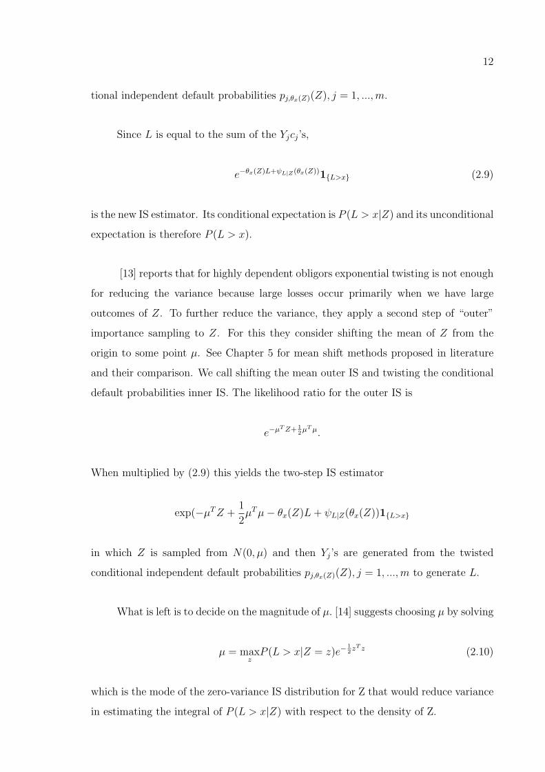
tional independent default probabilities pj,θx(Z)(Z), j = 1, ...,m.

Since L is equal to the sum of the Yjcj’s,

e−θx(Z)L+ψL|Z(θx(Z))1{L>x} (2.9)

is the new IS estimator. Its conditional expectation is P (L > x|Z) and its unconditional

expectation is therefore P (L > x).

[13] reports that for highly dependent obligors exponential twisting is not enough

for reducing the variance because large losses occur primarily when we have large

outcomes of Z. To further reduce the variance, they apply a second step of “outer”

importance sampling to Z. For this they consider shifting the mean of Z from the

origin to some point µ. See Chapter 5 for mean shift methods proposed in literature

and their comparison. We call shifting the mean outer IS and twisting the conditional

default probabilities inner IS. The likelihood ratio for the outer IS is

e−µTZ+ 1

2µTµ.

When multiplied by (2.9) this yields the two-step IS estimator

exp(−µTZ +1

2µTµ− θx(Z)L+ ψL|Z(θx(Z))1{L>x}

in which Z is sampled from N(0, µ) and then Yj’s are generated from the twisted

conditional independent default probabilities pj,θx(Z)(Z), j = 1, ...,m to generate L.

What is left is to decide on the magnitude of µ. [14] suggests choosing µ by solving

µ = maxzP (L > x|Z = z)e−

12zT z (2.10)

which is the mode of the zero-variance IS distribution for Z that would reduce variance

in estimating the integral of P (L > x|Z) with respect to the density of Z.

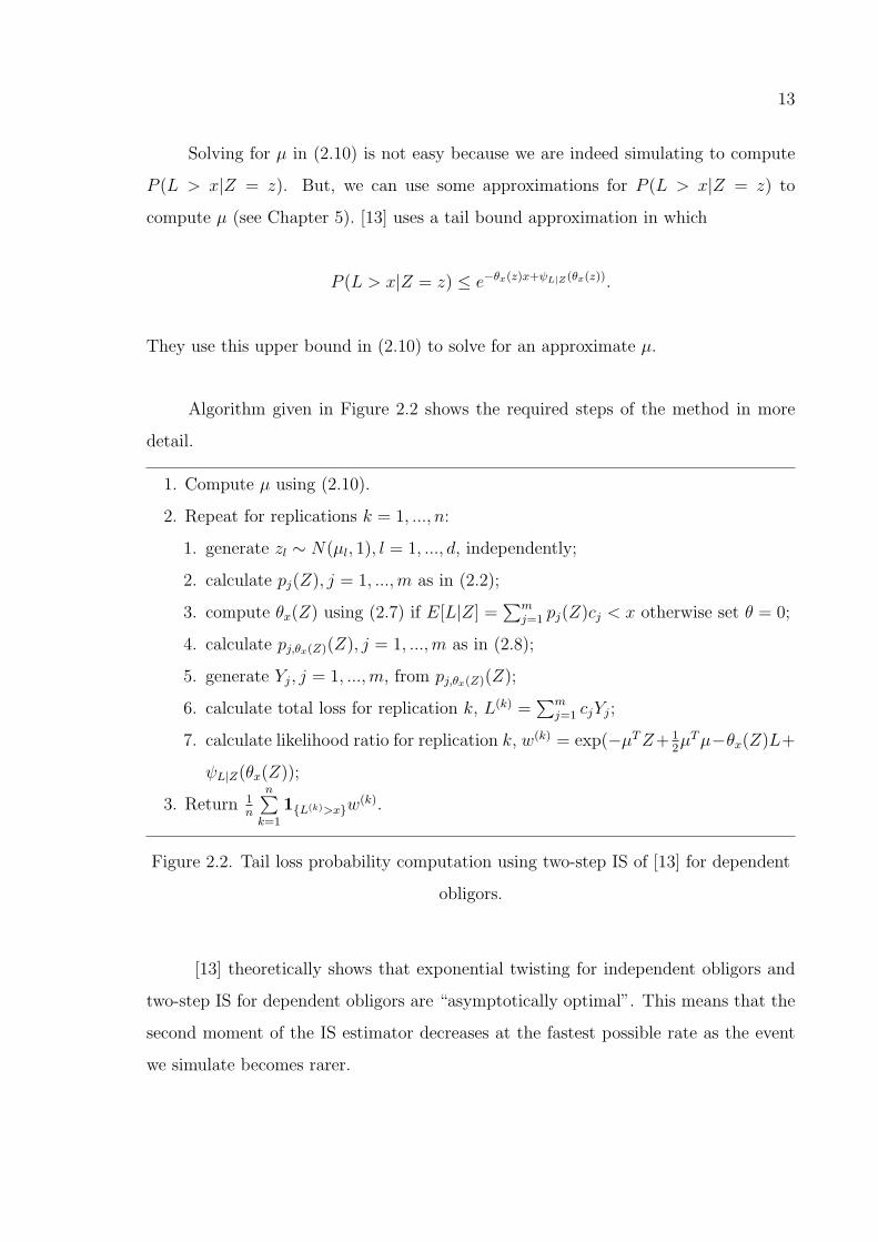
13

Solving for µ in (2.10) is not easy because we are indeed simulating to compute

P (L > x|Z = z). But, we can use some approximations for P (L > x|Z = z) to

compute µ (see Chapter 5). [13] uses a tail bound approximation in which

P (L > x|Z = z) ≤ e−θx(z)x+ψL|Z(θx(z)).

They use this upper bound in (2.10) to solve for an approximate µ.

Algorithm given in Figure 2.2 shows the required steps of the method in more

detail.

1. Compute µ using (2.10).


1. generate zl ∼ N(µl, 1), l = 1, ..., d, independently;

2. calculate pj(Z), j = 1, ...,m as in (2.2);

3. compute θx(Z) using (2.7) if E[L|Z] =∑m

j=1 pj(Z)cj < x otherwise set θ = 0;

4. calculate pj,θx(Z)(Z), j = 1, ...,m as in (2.8);

5. generate Yj, j = 1, ...,m, from pj,θx(Z)(Z);


j=1 cjYj;

7. calculate likelihood ratio for replication k, w(k) = exp(−µTZ+ 12µTµ−θx(Z)L+

ψL|Z(θx(Z));

3. Return 1n

n∑k=1

1{L(k)>x}w(k).

Figure 2.2. Tail loss probability computation using two-step IS of [13] for dependent

obligors.

[13] theoretically shows that exponential twisting for independent obligors and

two-step IS for dependent obligors are “asymptotically optimal”. This means that the

second moment of the IS estimator decreases at the fastest possible rate as the event

we simulate becomes rarer.

14

3. OPTIMAL IS FOR INDEPENDENT OBLIGORS

In this chapter, we assume that obligors default independently. This indepen-

dence assumption will allow the use use of the binomial distribution for the group

of obligors having the same default probability under the simplification of cj = 1 for

j = 1, ...,m for simulating the loss probabilities and expected shortfalls.

3.1. Exponential Twisting for Binomial Distribution

We can use the binomial distribution to simulate for the P (L > x) given that

obligors default independently, pj = p and cj = 1 for j = 1, ...,m. But the question is:

Can we use exponential twisting directly on this binomial distribution?

Since, L =∑m

j=1 cjYj =∑m

j=1 Yj, L is a random variable with binomial distribu-

tion. Thus

P (L > x) =m∑

j=bxc+1

(m

j

)pj(1− p)m−j.

Applying exponential twisting as IS, the new probability of default becomes

pθ =peθ

1 + p(eθ − 1),

and the likelihood ratio is e(−θL+ψ(θ)) where

ψ(θ) =m∑j=1

log(1 + p(eθ − 1))

= m log(1 + p(eθ − 1))

= log(1 + p(eθ − 1))m.

15

So, the new estimator for P (L > x) is

1{L>x}e−θL+log(1+pθ(eθ−1))m = (1 + p(eθ − 1))m1{L>x}e

−θL.

If we take the expectation of the new estimator under the new measure;

Eθ[(1 + p(eθ − 1))m1{L>x}e−θL]

= (1 + p(eθ − 1))me−θxEpθ [1{L>x}e−θ(L−x)]

= (1 + p(eθ − 1))me−θxEpθ [1{L−x}e−θ(L−x)]

= (1 + p(eθ − 1))me−θxm∑

j=bxc+1

(m

j

)pjθ(1− pθ)

m−je−θ(j−x)

=m∑

j=bxc+1

(m

j

)pjθ(1− pθ)

m−je−θ(j−x)(1 + p(eθ − 1))me−θx

=m∑

j=bxc+1

(m

j

)pjθ(1− pθ)

m−je−θj(1 + p(eθ − 1))m

=m∑

j=bxc+1

(m

j

)(peθ

1 + p(eθ − 1)

)j (1− peθ

1 + p(eθ − 1)

)m−je−θj(1 + p(eθ − 1))m

=m∑

j=bxc+1

(m

j

)pj

(1 + p(eθ − 1))j

(1 + p(eθ − 1)− peθ

1 + p(eθ − 1)

)m−j(1 + p(eθ − 1))m

=m∑

j=bxc+1

(m

j

)pj

(1 + p(eθ − 1))j(1− p)m−j

(1 + p(eθ − 1))m−j(1 + p(eθ − 1))m

=m∑

j=bxc+1

(m

j

)pj(1− p)m−j 1

(1 + p(eθ − 1))m(1 + p(eθ − 1))m

=m∑

j=bxc+1

(m

j

)pj(1− p)m−j.

It is nothing but P (L > x). So, the new estimator is an unbiased estimator of P (L > x).

Then, we try to find the θ that will minimize the second moment of the estimator

16

Table 3.1. Portfolio composition (one obligor case)

Exposure level (c) Default rate (p)

103 0.01

for P (L > x). The second moment of the new estimator is

M2(x, θ) = Eθ[e−2θL+2ψ(θ)1{L>x}

]≤ exp(−2θx+ 2ψ(θ)).

To make the optimization problem simple, we minimize the upper bound. Thus,

ψ(θ)′= x. (3.1)

The solution to (3.1) is θ = log( x(1−p)p(m−x)

). So, if E[L] = mp < x then θ = log( x(1−p)p(m−x)

)

otherwise θ = 0.

3.2. Optimal IS Probabilities

We concentrate on a small number of groups of obligors to give optimal IS proba-

bilities. But, this is not a weird assumption. For example, [17] make use of eight group

of ratings in his model. We want to see the percentage difference of variances in using

optimal and “asymptotically optimal” IS in this section.

3.2.1. One Obligor Case

We first of all consider the simplest case; there is only one obligor in our portfolio.

Portfolio composition is given in Table 3.1. The loss distribution for this portfolio is

given in Table 3.2. We should consider the case where 0 < x < 103 so that P (L > x)

is different than zero and 1.

17

Table 3.2. Loss Distribution for the portflio (one obligor case)

i Loss (Li) Probability of loss (P (Li))

1 103 0.01

2 0 0.99

3.2.1.1. Computing Tail Loss Probability. Our aim is to compute P (L > x). In this

simplest case of a portfolio we have an analytical solution

P (L > x) =2∑i=1

1{Li>x}P (Li) = p

where Li is the loss distribution value which has probability greater than zero.

Naive and IS simulation algorithms are given in Figures 3.1 and 3.2. In the

algorithm given in Figure 3.2, pnew is the IS default probability for the obligor.


1. generate Y from p;

2. calculate total loss for replication k, L(k) = cY ;

2. Return 1n

n∑k=1

1{L(k)>x}.

Figure 3.1. Naive simulation algorithm for P (L > x) (one obligor case)


1. generate Y from pnew;


3. calculate likelihood ratio for replication k, w(k) = ppnew

;

2. Return 1n

n∑k=1

1{L(k)>x}w(k).

Figure 3.2. IS algorithm for P (L > x) (one obligor case)

18

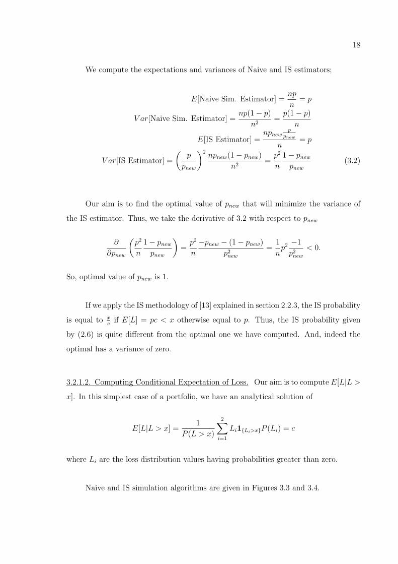
We compute the expectations and variances of Naive and IS estimators;

E[Naive Sim. Estimator] =np

n= p

V ar[Naive Sim. Estimator] =np(1− p)

n2=p(1− p)

n

E[IS Estimator] =npnew

ppnew

n= p

V ar[IS Estimator] =

(p

pnew

)2npnew(1− pnew)

n2=p2

n

1− pnewpnew

(3.2)

Our aim is to find the optimal value of pnew that will minimize the variance of

the IS estimator. Thus, we take the derivative of 3.2 with respect to pnew

∂

∂pnew

(p2

n

1− pnewpnew

)=p2

n

−pnew − (1− pnew)

p2new

=1

np2 −1

p2new

< 0.

So, optimal value of pnew is 1.

If we apply the IS methodology of [13] explained in section 2.2.3, the IS probability

is equal to xc

if E[L] = pc < x otherwise equal to p. Thus, the IS probability given

by (2.6) is quite different from the optimal one we have computed. And, indeed the

optimal has a variance of zero.

3.2.1.2. Computing Conditional Expectation of Loss. Our aim is to compute E[L|L >

x]. In this simplest case of a portfolio, we have an analytical solution of

E[L|L > x] =1

P (L > x)

2∑i=1

Li1{Li>x}P (Li) = c

where Li are the loss distribution values having probabilities greater than zero.

Naive and IS simulation algorithms are given in Figures 3.3 and 3.4.

19


1. generate Y from p;


2. Return

∑nk=1 L

(k)1{L(k)>x}∑nk=1 1{L(k)>x}

.

Figure 3.3. Naive simulation algorithm for E[L|L > x] (one obligor case)


1. generate Y from pnew;


3. calculate likelihood ratio for replication k, w(k) = ppnew

;

2. Return

∑nk=1 L

(k)w(k)1{L(k)>x}∑nk=1w

(k)1{L(k)>x}.

Figure 3.4. IS algorithm for E[L|L > x] (one obligor case)

We compute the expectations and variances of Naive and IS estimators;

E[Naive Sim. Estimate] =nc1p

nP (L > x)=

c1p

P (L > x)

V ar[Naive Sim. Estimate] =nc2

1p(1− p)n2P (L > x)2

=c2

1p(1− p)nP (L > x)2

E[IS Estimate] =nc1pnew

ppnew

nP (L > x)=

c1p

P (L > x)

V ar[IS Estimate] =

(pc1

pnew

)2npnew(1− pnew)

n2P (L > x)2=

c21p

2

nP (L > x)2

1− pnewpnew

. (3.3)

Our aim is to find the optimal value of pnew that will minimize the variance of

the IS estimator. Thus, we take the derivative of 3.3 with respect to pnew

∂

∂pnew

(p2c2

1

n

1− pnewpnew

)=p2c2

1

n

−pnew − (1− pnew)

p2new

=p2c2

1

n

−1

p2new

< 0.

Thus, optimal value of pnew is 1.

20

Table 3.3. Portfolio composition (independent two obligors)

Exposure level (cj, j = 1, 2) Default rate (pk, k = A,B)

Obligor A 103 0.01

Obligor B 105 0.05

Table 3.4. Loss Distribution for the portio (independent two obligors)

i Loss (Li) Probability (P (Li))

1 c1 + c2 = 208 0.01 ∗ 0.05 = 0.0005

2 c2 = 105 (1− 0.01) ∗ 0.05 = 0.0495

3 c1 = 103 0.01 ∗ (1− 0.05) = 0.0095

4 0 (1− 0.01) ∗ (1− 0.05) = 0.9405

[12] uses the same exponential twisting probabilities for expected shortfall con-

tributions with tail loss probability computation. Thus, from the previous section we

have seen that the exponential twisting probability is quite different from the optimal

probability 1.

3.2.2. Two Obligors Case

In this section, we consider the two obligors case. They default independently.

The portfolio composition is given in Table 3.3. The loss distribution for the portfolio

is given in Table 3.4.

3.2.2.1. Computing Tail Loss Probability. Our aim is to compute P (L > x). It has

the analytical solution

P (L > x) =4∑i=1

1{Li>x}P (Li)

where Li are the loss distribution values having probabilities greater than zero.

21

Naive and IS simulation algorithms are given in Figures 3.5 and 3.6 to compute

P (L > x).


1. generate Y1 from pA and Y2 from pB;

2. calculate total loss for replication k, L(k) = c1Y1 + c2Y2;

2. Return 1n

n∑k=1

1{L(k)>x}.

Figure 3.5. Naive simulation algorithm for P (L > x) (two independent obligors case)


1. generate Y1 from pnew,A and Y2 from pnew,B;


3. calculate likelihood ratio for replication k,

w(k) =(

pApnew,A

)Y1(

1−pA1−pnew,A

)1−Y1(

pBpnew,B

)Y2(

1−pB1−pnew,B

)1−Y2

;

2. Return 1n

n∑k=1

1{L(k)>x}w(k).

Figure 3.6. IS algorithm for P (L > x) (two independent obligors case)

If max{c1 , c2} < x < c1 +c2, the only possibility of L > x is the case where two of

the obligors default at the same time. Since, the defaults are independent, the problem

simplifies to the one company case where the default probability is the product of two

default probabilities of the obligors. So, the multiplication of default probabilities in

new measure should be equal to 1 for the optimal IS. Thus, pnew,A = pnew,B = 1 are

the optimal values of the new default probabilities for this case.

If c1 ≤ x ≤ c2;

E[Naive Sim. Estimator] =n [(1− pA)pB + pApB]

n= pB

V ar[Naive Sim. Estimator] =1

n

[pB − p2

B

]E[IS Estimator] =

n(pnew,Apnew,B

pApnew,A

pBpnew,B

+ (1− pnew,A)pnew,B1−pA

1−pnew,ApB

pnew,B

)n

= pB.

22

V ar[IS Estimator] =n

n2

(pnew,Apnew,B

(pA

pnew,A

pBpnew,B

)2

+

(1− pnew,A)pnew,B

(1− pA

1− pnew,ApB

pnew,B

)2

− p2B

)

=1

n

(p2Ap

2B

pnew,Apnew,B+

(1− pA)2 p2B

(1− pnew,A)pnew,B− p2

B

)

=1

n

(p2Ap

2B(1− pnew,A) + (1− pA)2 p2

Bpnew,Apnew,Apnew,B(1− pnew,A)

− p2B

)

=p2B

n

(p2A(1− pnew,A) + (1− pA)2 pnew,A

pnew,Apnew,B(1− pnew,A)− 1

)

=p2B

n

(p2A − p2

Apnew,A + pnew,A − 2pApnew,A + p2Apnew,A

pnew,Apnew,B(1− pnew,A)− 1

)=

p2B

n

(p2A + pnew,A − 2pApnew,Apnew,Apnew,B(1− pnew,A)

− 1

)

To minimize V ar[IS Estimator];

∂V ar[IS Estimator]

∂pnew,B=

p2B

n

− (p2A + pnew,A − 2pApnew,A) pnew,A(1− pnew,A)

(pnew,Apnew,B(1− pnew,A))2

=p2B

n

− (p2A + pnew,A − 2pApnew,A)

pnew,Ap2new,B(1− pnew,A)

So, ∂V ar[IS Estimator]∂pnew,B

≤ 0 if (p2A + pnew,A − 2pApnew,A) ≥ 0 which necessitates pnew,A ≥

−p2A1−2pA

for pA < 0.5 and pnew,A ≤−p2A

1−2pAfor pA > 0.5. Since, these conditions are always

satisfied, minimum is is attained for pnew,B = 1.

Then, if we put pnew,B = 1 into the equation and take the derivative with respect

to pnew,A;

23

∂V ar[IS Estimator]

∂pnew,A=

p2B

n

(2pA − 1

p2new,A − pnew,A

+pnew,A − 2pnew,ApA + p2

A

p3new,A − p2

new,A

+

pnew,A − 2pnew,ApA + p2A

pnew,A − 2p2new,A + p3

new,A

)= 0.

Solution is:

{pA,

pA2pA−1

}if pA 6= 1

2

{pA} if pA = 12

.

To summarize, for all cases pA <12, pA >

12

and pA = 12, the optimal solution is

pnew,A = pA and pnew,B = 1.

Thus, the optimal solution is pnew,B = 1 and pnew,A = pA. This is nothing but

the variance of the one company case where the default probability is equivalent to pB.

Note that c2 ≤ x ≤ c1 is the same as the previous case but this time we should

only change default probability of company A instead of B. So, the optimal solution

is pnew,A = 1 and pnew,B = pB.

If x < min{c1, c2};

E[Naive Sim. Estimator] =n [1− (1− pA)(1− pB)]

n

= pA + pB − pApB = p

V ar[Naive Sim. Estimator] =1

n

[p− p2

]

24

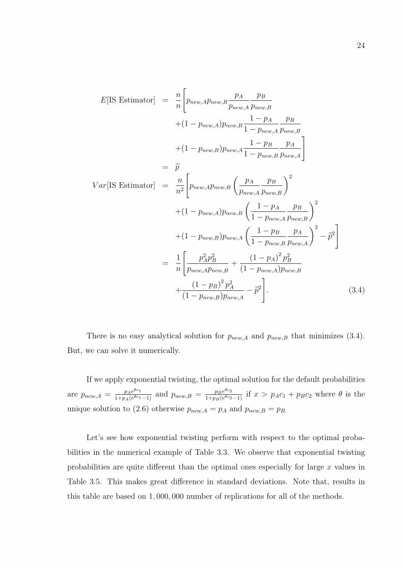
E[IS Estimator] =n

n

[pnew,Apnew,B

pApnew,A

pBpnew,B

+(1− pnew,A)pnew,B1− pA

1− pnew,ApB

pnew,B

+(1− pnew,B)pnew,A1− pB

1− pnew,BpA

pnew,A

]= p


n2

[pnew,Apnew,B

(pA

pnew,A

pBpnew,B

)2

+(1− pnew,A)pnew,B

(1− pA

1− pnew,ApB

pnew,B

)2

+(1− pnew,B)pnew,A

(1− pB

1− pnew,BpA

pnew,A

)2

− p2

]

=1

n

[p2Ap

2B

pnew,Apnew,B+

(1− pA)2 p2B

(1− pnew,A)pnew,B

+(1− pB)2 p2

A

(1− pnew,B)pnew,A− p2

]. (3.4)

There is no easy analytical solution for pnew,A and pnew,B that minimizes (3.4).

But, we can solve it numerically.

If we apply exponential twisting, the optimal solution for the default probabilities

are pnew,A = pAeθc1

1+pA(eθc1−1)and pnew,B = pBe

θc2

1+pB(eθc2−1)if x > pAc1 + pBc2 where θ is the

unique solution to (2.6) otherwise pnew,A = pA and pnew,B = pB.

Let’s see how exponential twisting perform with respect to the optimal proba-

bilities in the numerical example of Table 3.3. We observe that exponential twisting

probabilities are quite different than the optimal ones especially for large x values in

Table 3.5. This makes great difference in standard deviations. Note that, results in

this table are based on 1, 000, 000 number of replications for all of the methods.

25

Table 3.5. Optimal (OP) and exponential twisting probabilities (ETP) and

corresponding standard deviations (sd) to compute P (L > x) (Two independent

obligors case).

x OP sd (O) ETP sd (ET) sd (naive)

pnew,A pnew,B pnew,A pnew,B

120 1 1 4.07 ∗ 10−18 0.377 0.773 7.80 ∗ 10−7 2.22 ∗ 10−5

110 1 1 4.08 ∗ 10−18 0.324 0.729 8.99 ∗ 10−7 2.22 ∗ 10−5

104 0.010 1 9.23 ∗ 10−16 0.295 0.701 4.96 ∗ 10−5 2.18 ∗ 10−4

100 0.250 0.750 4.76 ∗ 10−5 0.276 0.681 4.95 ∗ 10−5 2.37 ∗ 10−4

90 0.250 0.750 4.76 ∗ 10−5 0.233 0.629 5.09 ∗ 10−5 2.36 ∗ 10−4


x]. It has an analytical solution of

E[L|L > x] =1

P (L > x)

4∑i=1

Li1{Li>x}P (Li)

where Li are the loss distribution values which have probabilities greater than zero.


E[L|L > x].


1. generate Y1 from pA and Y2 from pB;


2. Return

∑nk=1 L

(k)1{L(k)>x}∑nk=1 1{L(k)>x}

Figure 3.7. Naive simulation algorithm for E[L|L > x] (two independent obligors

case)

If max{c1 , c2} < x < c1 +c2, the only possibility of L > x is the case where two of

the bonds default at the same time. Since, the defaults are independent, the problem

26


1. generate Y1 from pnew,A and Y2 from pnew,B;


3. calculate w(k) =(

pApnew,A

)Y1(

1−pA1−pnew,A

)1−Y1(

pBpnew,B

)Y2(

1−pB1−pnew,B

)1−Y2

2. Return

∑nk=1 L


(k)1{L(k)>x}.

Figure 3.8. IS algorithm for E[L|L > x] (two independent obligors case)

simplifies to the one company case where default probability is the multiplication of

two default probabilities of the obligors. So, the multiplication of default probabilities

in new measure should be equal to 1 for the optimal IS. Thus, pnew,A = pnew,B = 1 are

the optimal values of new default probabilities for this case.

If c1 ≤ x ≤ c2;

E[Naive Sim. Estimator] =c2(1− pA)pB + (c1 + c2)pApB

P (L > x)=c2pB + c1pApBP (L > x)

E[IS Estimator] =1

P (L > x)

((c1 + c2)pnew,Apnew,B

pApnew,A

pBpnew,B

+c2(1− pnew,A)pnew,B1− pA

1− pnew,ApB

pnew,B

)=

c2pB + c1pApBP (L > x)

27


P (L > x)2n2

[(c1 + c2)2pnew,Apnew,B

(pA

pnew,A

pBpnew,B

)2

+c22(1− pnew,A)pnew,B

(1− pA

1− pnew,ApB

pnew,B

)2

− (c2pB + c1pApB)2

]

=1

nP (L > x)2

[(c1 + c2)2 p2

A

pnew,A

p2B

pnew,B

+c22

(1− pA)2

1− pnew,Ap2B

pnew,B− (c2pB + c1pApB)2

]. (3.5)

If x < min{c1, c2};

E[Naive Sim. Estimator] =1

P (L > x)

[c1(1− pB)pA + c2(1− pA)pB + (c1 + c2)pApB

]=

c1pA + c2pBP (L > x)

E[IS Estimator] =1

P (L > x)

[(c1 + c2)pnew,Apnew,B

pApnew,A

pBpnew,B

+c2(1− pnew,A)pnew,B1− pA

1− pnew,ApB

pnew,B

+c1(1− pnew,B)pnew,A1− pB

1− pnew,BpA

pnew,A

]=

c1pA + c2pBP (L > x)

28


standard deviations (sd) to compute E[L|L > x] (Two independent obligors case).


pnew,A pnew,B pnew,A pnew,B

120 1 1 4.22 ∗ 10−12 0.377 0.773 0.324 9.30

110 1 1 4.22 ∗ 10−12 0.324 0.729 0.374 9.30

104 0.020 1.000 2.90 ∗ 10−4 0.295 0.701 0.103 0.464

100 0.248 0.753 0.082 0.276 0.681 0.086 0.422

90 0.248 0.753 0.082 0.233 0.629 0.089 0.421


P (L > x)2n2

[(c1 + c2)2pnew,Apnew,B

(pA

pnew,A

pBpnew,B

)2

+c22(1− pnew,A)pnew,B

(1− pA

1− pnew,ApB

pnew,B

)2

+c21(1− pnew,B)pnew,A

(1− pB

1− pnew,BpA

pnew,A

)2

− (c1pA + c2pB)2

]

=1

nP (L > x)2

[(c1 + c2)2 p2

A

pnew,A

p2B

pnew,B+ c2

2

(1− pA)2

1− pnew,Ap2B

pnew,B

+c21

(1− pB)2

1− pnew,Bp2A

pnew,A− (c1pA + c2pB)2

]. (3.6)

We numerically solve (3.5) and (3.6) for the optimal probabilities. Table 3.6

presents how exponential twisting probabilities perform compared to the optimal prob-

abilities when computing E[L|L > x] in the numerical example of Table 3.3. We ob-

serve that exponential twisting probabilities are quite different than the optimal ones

especially for large x values in Table 3.6. This makes great difference in standard devi-

ations. Note that, results in this table are based on 1, 000, 000 number of replications

for all of the methods.

29

3.2.3. One Homogeneous Group of Obligors

We show that we can use binomial distribution in IS of [13] to compute P (L > x)

for an homogeneous portfolio in section 3.1. But, the question is what is the perfor-

mance of using this approach to compute P (L > x) and E[L|L > x] compared to the

optimal IS strategy.

Let’s take pj = p and cj = 1 from j = 1, ...,m so that L =∑m

j=1 cjYj =∑m

j=1 Yj

is a random variable with binomial distribution with parameters p and m.

3.2.3.1. Computing Tail Loss Probability. Our aim is to compute P (L > x) which has

an analytical solution of

P (L > x) =m∑

i=bxc+1

(m

i

)pi(1− p)m−i

under the assumptions we make.


P (L > x).


1. generate L(k) from binomial distribution with parameters p and m;

2. Return 1n

n∑k=1

1{L(k)>x}.

Figure 3.9. Naive simulation algorithm for P (L > x) (One homogeneous group of

obligors case)

It is easy to show the unbiasedness of IS estimator. Our aim is to choose a pnew

that will minimize the variance of the IS estimator.

30


1. generate L(k) from binomial distribution with parameters pnew and m;

2. calculate likelihood ratio for replication k, w(k) =(

ppnew

)L(k) (1−p

1−pnew

)m−L(k)

;

2. Return 1n

n∑k=1

1{L(k)>x}w(k).

Figure 3.10. IS algorithm for P (L > x) (One homogeneous group of obligors case)

The variance of the IS estimator is

1

n

[m∑

i=bxc+1

(p

pnew

)2i(1− p

1− pnew

)2m−2i(m

i

)pinew(1− pnew)m−i

−

m∑i=bxc+1

(m

i

)pi(1− p)m−i

2]

=1

n

m∑i=bxc+1

(m

i

)p2i (1− p)2m−2i

pinew (1− pnew)m−i−

m∑i=bxc+1

(m

i

)pi(1− p)m−i

2 .Since, the last term (square of the expectation of the naive and IS estimator) does

not depend on pnew, it is enough to minimize the first term (second moment of the

estimator). Thus, our optimization problem is

minpnew

m∑i=bxc+1

(m

i

)p2i (1− p)2m−2i

pinew (1− pnew)m−i

which we solve numerically.

Let’s see how exponential twisting probabilities perform compared to the optimal

probabilities in a numerical example given in Table 3.7. We observe that exponential

twisting probabilities are quite close to the optimal ones for x > 10. This is why we

don’t see much difference in standard deviations. Note that, results in this table are

based on 1, 000, 000 number of replications for all of the methods.

31

Table 3.7. Optimal and exponential twisting IS probabilities and corresponding

standard deviations (sd) for the parameter values of m = 100 and p = 0.1 to compute

P (L > x).


30 0.311 1.51 ∗ 10−11 0.300 1.53 ∗ 10−11 7.78 ∗ 10−8

25 0.261 9.17 ∗ 10−9 0.250 9.35 ∗ 10−9 2.02 ∗ 10−6

20 0.212 1.54 ∗ 10−6 0.200 1.58 ∗ 10−6 2.84 ∗ 10−5

15 0.164 5.80 ∗ 10−5 0.150 6.15 ∗ 10−5 1.96 ∗ 10−4

10 0.122 3.57 ∗ 10−4 0.100 4.93 ∗ 10−4 4.93 ∗ 10−4


x] which has an analytical solution of

E[L|L > x] =1

P (L > x)

m∑i=bxc+1

i

(m

i

)pi(1− p)m−i.

Naive and IS simulation algorithms are given in Figures 3.11 and 3.12.


1. generate L(k) from binomial distribution with parameters p and m;

2. Return

∑nk=1 L

(k)1{L(k)>x}∑nk=1 1{L(k)>x}

.

Figure 3.11. Naive simulation algorithm for E[L|L > x] (One homogeneous group of

obligors case)

Under the assumption of large number of replications, the denominator of the

ratio becomes P (L > x). So, it is easy to show the asymptotically unbiasedness of

the IS estimator. Our aim is to choose a pnew that will minimize the variance of IS

estimator.

32


1. generate L(k) from binomial distribution with parameters pnew and m;


3. calculate likelihood ratio for replication k, w(k) =(

ppnew

)L(k) (1−p

1−pnew

)m−L(k)

;

2. Return

∑nk=1 L


(k)1{L(k)>x}.

Figure 3.12. IS algorithm for E[L|L > x] (One homogeneous group of obligors case)

The asymptotic variance of the IS estimator is

1

nP (L > x)2

[m∑

i=bxc+1

i2(

p

pnew

)2i(1− p

1− pnew

)2m−2i(m

i

)pinew(1− pnew)m−i −

m∑i=bxc+1

i

(m

i

)pi(1− p)m−i

2]

=1

nP (L > x)2

m∑i=bxc+1

(m

i

)i2

p2i (1− p)2m−2i

pinew (1− pnew)m−i−

m∑i=bxc+1

(m

i

)ipi(1− p)m−i

2 .

Since, the last term (square of the expectation of the naive and IS estimator)

does not depend on pnew, it is enough to solve for pnew that will minimize the first term

(second moment of the estimator) to minimize the variance. Thus, our optimization

problem is

minpnew

m∑i=bxc+1

(m

i

)i2

p2i (1− p)2m−2i

pinew (1− pnew)m−i


Let’s see how exponential twisting probabilities perform compared to the optimal

probabilities in a numerical example given in Table 3.8. We observe that exponential

twisting probabilities are quite close to the optimal ones for x > 10. This is why we

don’t see much difference in standard deviations. Note that, results in this table are

33


standard deviations (sd) for the parameter values of m = 100 and p = 0.1 to compute

E[L|L > x].


30 0.311 0.083 0.300 0.085 402.640

25 0.261 0.064 0.250 0.065 13.051

20 0.212 0.046 0.200 0.047 0.761

15 0.165 0.029 0.150 0.030 0.085

10 0.125 0.016 0.100 0.020 0.020

based on 1, 000, 000 number of replications for all of the methods.

3.2.4. Two Homogenous Groups of Obligors

The last case of this section is to have two homogenous group of obligors. Again,

all obligors default independently. We assume that for the first group A, cj = 1, j =

1, ...,mA and the second B, cj = 1, j = 1, ...,mB. Moreover, we assume that x takes

integer values.

3.2.4.1. Computing Tail Loss Probability. Our aim is to compute P (L > x) which has

an analytical solution of

P (L > x) =

mA∑i=0

(mA

i

)piA(1− pA)mA−i

mB∑j=[bxc−i+1]+

(mB

j

)pjB(1− pB)mB−j

where [x]+ = max(0, x).


P (L > x).

Our aim is to minimize the variance of IS estimator to compute the optimal IS

34


1. generate L(k)A from binomial distribution with parameters pA and mA and L

(k)B

from binomial distribution with parameters pB and mB;

2. calculate total loss for replication k, L(k) = L(k)A + L

(k)B .

2. Return 1n

n∑k=1

1{L(k)>x}.

Figure 3.13. Naive simulation algorithm for P (L > x) (Two homogeneous groups of

obligors case)


1. generate L(k)A from binomial distribution with parameters pnew,A and mA and

L(k)B from binomial distribution with parameters pnew,B and mB;


w(k) =(

pApnew,A

)L(k)A(

1−pA1−pnew,A

)mA−L(k)A(

pBpnew,B

)L(k)B(

1−pB1−pnew,B

)mB−L(k)B

;

2. Return 1n

n∑k=1

1{L(k)>x}w(k).

Figure 3.14. IS algorithm for P (L > x) (Two homogeneous groups of obligors case)

35

probabilities. The resulting minimization problem is

minpnew,A,pnew,B

mA∑i=0

(mA

i

)pinew,A(1− pnew,A)mA−i

mB∑j=[bxc−i+1]+

(mB

j

)pjnew,B(1− pnew,B)mB−j

∗(

pApnew,A

)2i(1− pA

1− pnew,A

)2mA−2i(pB

pnew,B

)2j (1− pB

1− pnew,B

)2mB−2j

= minpnew,A,pnew,B

mA∑i=0

(mA

i

)p2iA(1− pA)2mA−2i

pinew,A(1− pnew,A)mA−i

mB∑j=[bxc−i+1]+

(mB

j

)

∗ p2jB (1− pB)2mB−2j

pjnew,B(1− pnew,B)mB−j


We give a numerical example to have an idea about how close the optimal and

exponential twisting probabilities and corresponding variances are in Table 3.9. Note

that, results in this table are based on 1, 000, 000 number of replications for all of

the methods. Furthermore, in Figures 3.15 to 3.20, we not only give optimal and

exponential twisting probabilities proposed by [13] (represented as +) but also contour

lines of variances and possible exponential twisting pairs of probabilities for P (L > x)

for the parameters in Table 3.9. Note that we use R [30] for plotting the graphs. We

observe that exponential twisting could be used to compute the optimal probabilities

from the figures. However, exponential twisting probabilities proposed by [13] are far

away from the optimal probabilities when the number of obligors is small and the tail

loss probability we simulate is not very small, as they use the tail approximation of the

variance in optimizing the exponential twisting parameter (θ). As it can be seen from

our figures and Table 3.9 exponential twisting is asymptotically optimal. That is when

the number of obligors increase and tail loss probability we simulate becomes smaller

(x increase), exponential twisting probabilities proposed by [13] are quite close to the

optimal ones.

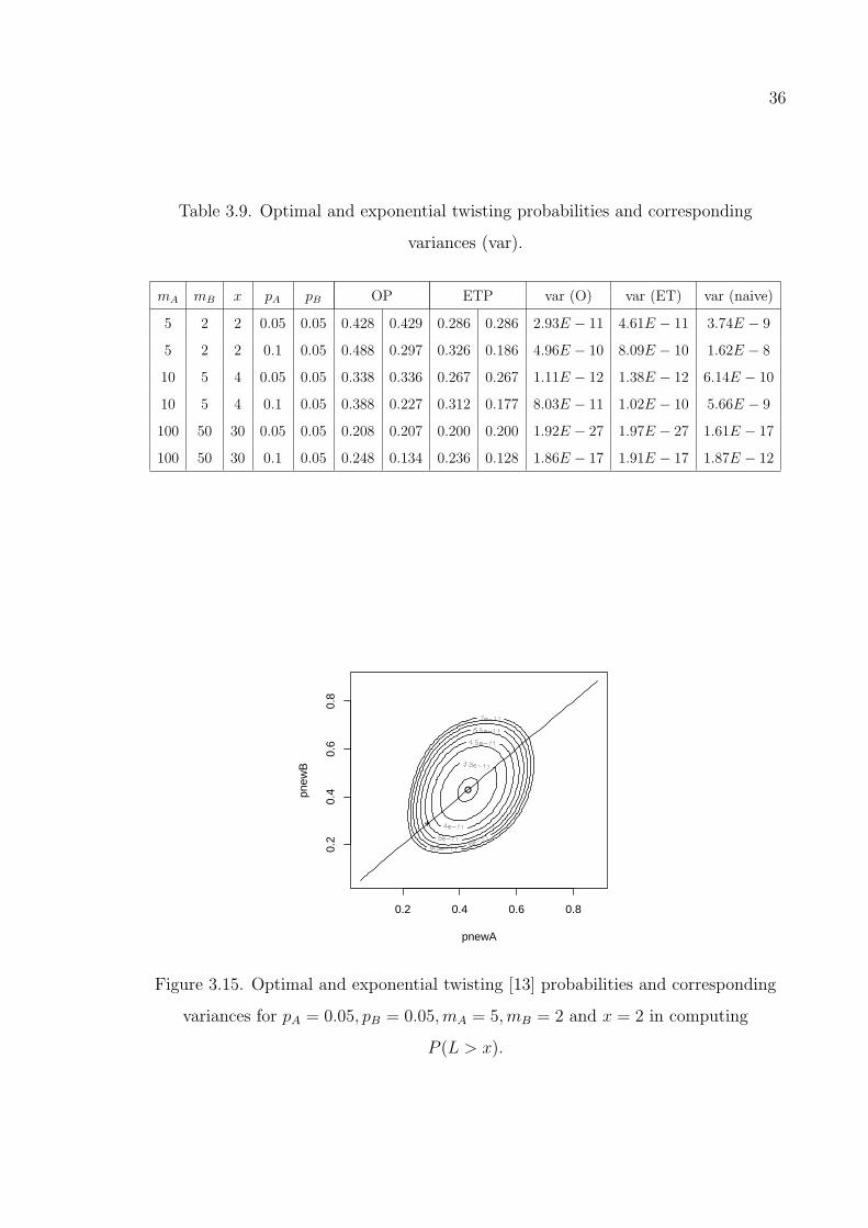
36


variances (var).

mA mB x pA pB OP ETP var (O) var (ET) var (naive)

5 2 2 0.05 0.05 0.428 0.429 0.286 0.286 2.93E − 11 4.61E − 11 3.74E − 9

5 2 2 0.1 0.05 0.488 0.297 0.326 0.186 4.96E − 10 8.09E − 10 1.62E − 8

10 5 4 0.05 0.05 0.338 0.336 0.267 0.267 1.11E − 12 1.38E − 12 6.14E − 10

10 5 4 0.1 0.05 0.388 0.227 0.312 0.177 8.03E − 11 1.02E − 10 5.66E − 9

100 50 30 0.05 0.05 0.208 0.207 0.200 0.200 1.92E − 27 1.97E − 27 1.61E − 17

100 50 30 0.1 0.05 0.248 0.134 0.236 0.128 1.86E − 17 1.91E − 17 1.87E − 12

0.2 0.4 0.6 0.8

0.2

0.4

0.6

0.8

pnewA

pnew

B

●

+

Figure 3.15. Optimal and exponential twisting [13] probabilities and corresponding

variances for pA = 0.05, pB = 0.05,mA = 5,mB = 2 and x = 2 in computing

P (L > x).

37

0.2 0.4 0.6 0.8

0.2

0.4

0.6

0.8

pnewA

pnew

B

●

+


variances for pA = 0.1, pB = 0.05,mA = 5,mB = 2 and x = 2 in computing P (L > x).

0.2 0.4 0.6 0.8

0.2

0.4

0.6

0.8

pnewA

pnew

B

●

+



P (L > x).

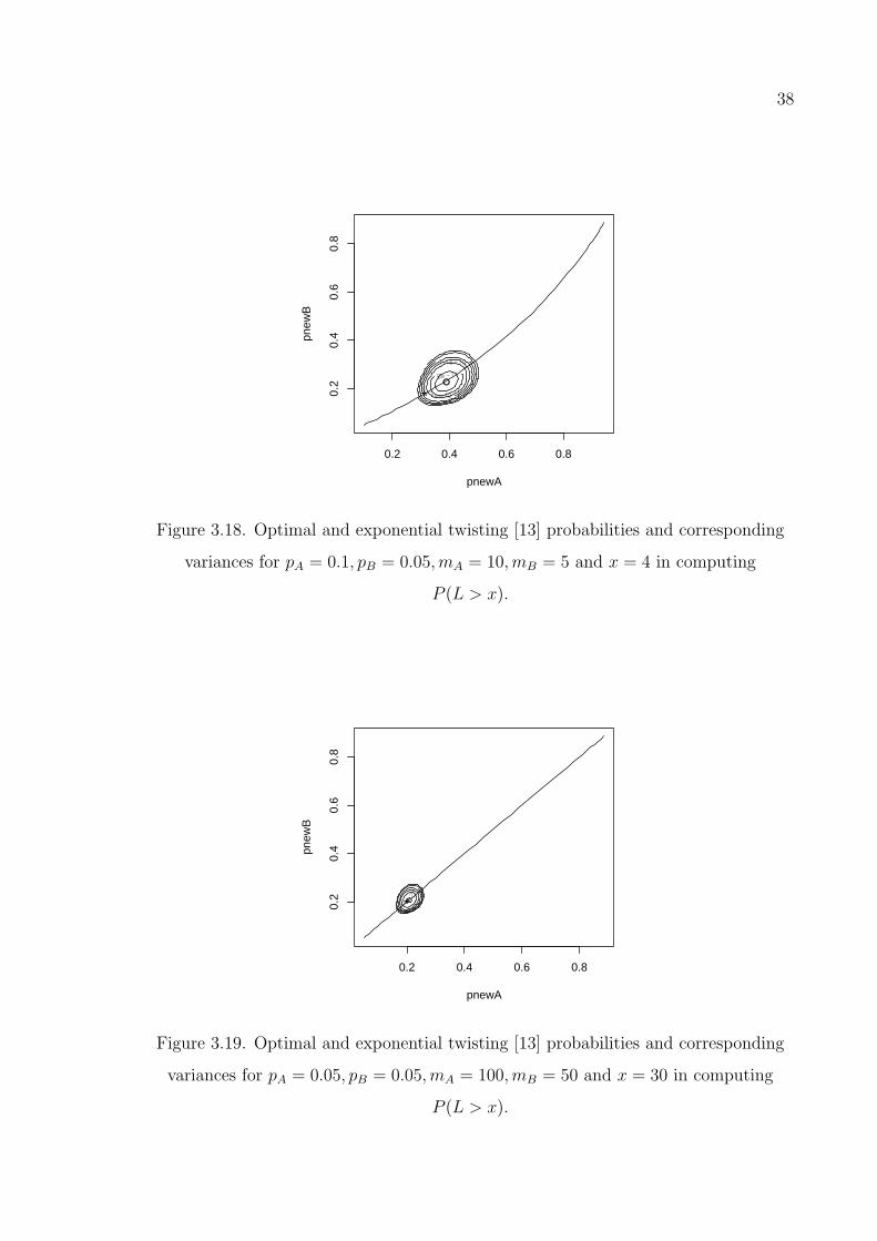
38

0.2 0.4 0.6 0.8

0.2

0.4

0.6

0.8

pnewA

pnew

B

●

+



P (L > x).

0.2 0.4 0.6 0.8

0.2

0.4

0.6

0.8

pnewA

pnew

B

+



P (L > x).

39

0.2 0.4 0.6 0.8

0.2

0.4

0.6

0.8

pnewA

pnew

B

●+



P (L > x).


x] which has an analytical solution of

E(L|L > x)

=1

P (L > x)

mA∑i=0

mB∑j=[bxc−i+1]+

(i+ j)

(mA

i

)piA(1− pA)mA−i

(mB

j

)pjB(1− pB)mB−j.


E[L|L > x].

Under the assumption of a large number of replications, the denominator of the

ratio becomes P (L > x). So, it is easy to show the asymptotical unbiasedness of the

IS estimator. Our aim is to choose the pnew,A and pnew,B pair that will minimize the

variance of IS estimator.

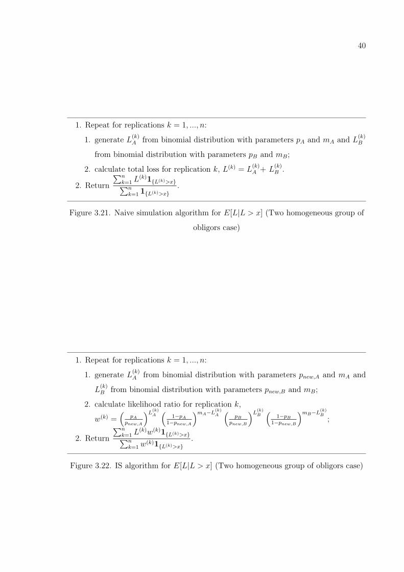
40


1. generate L(k)A from binomial distribution with parameters pA and mA and L

(k)B

from binomial distribution with parameters pB and mB;

2. calculate total loss for replication k, L(k) = L(k)A + L

(k)B .

2. Return

∑nk=1 L

(k)1{L(k)>x}∑nk=1 1{L(k)>x}

.

Figure 3.21. Naive simulation algorithm for E[L|L > x] (Two homogeneous group of

obligors case)


1. generate L(k)A from binomial distribution with parameters pnew,A and mA and

L(k)B from binomial distribution with parameters pnew,B and mB;


w(k) =(

pApnew,A

)L(k)A(

1−pA1−pnew,A

)mA−L(k)A(

pBpnew,B

)L(k)B(

1−pB1−pnew,B

)mB−L(k)B

;

2. Return

∑nk=1 L


(k)1{L(k)>x}.

Figure 3.22. IS algorithm for E[L|L > x] (Two homogeneous group of obligors case)

41

The resulting minimization problem is

minpnew,A,pnew,B

mA∑i=0

mB∑j=[bxc−i+1]+

(i+ j)2

(pA

pnew,A

)2i(1− pA

1− pnew,A

)2mA−2i

∗

(pB

pnew,B

)2j (1− pB

1− pnew,B

)2mB−2j (mA

i

)pinew,A(1− pnew,A)mA−i ∗(

mB

j

)pjnew,B(1− pnew,B)mB−j

= minpnew,A,pnew,B

mA∑i=0

(mA

i

)p2iA(1− pA)2mA−2i

pinew,A(1− pnew,A)mA−i

mB∑j=[bxc−i+1]+

(i+ j)2

(mB

j

)∗

p2jB (1− pB)2mB−2j

pjnew,B(1− pnew,B)mB−j


We give a numerical example to have an idea about how close the optimal and

exponential twisting probabilities proposed by [13] and corresponding variances are

in Table 3.10. Note that, results in this table are based on 1, 000, 000 number of

replications for all of the methods. Furthermore, in Figures 3.23 to 3.28, we not

only give optimal and exponential twisting probabilities proposed by [13] (represented

as +) but also contour lines of variances and possible exponential twisting pairs of

probabilities for E[L|L > x] for the parameters in Table 3.10. Since, we use the same

exponential twisting probabilities of [13] for both P (L > x) and E[L|L > x], and also

optimal probabilities we compute are nearly the same for both cases, the comments we

made for P (L > x) are completely valid for this section as well.

We give more numerical results in Table A.1 to A.4. Please note that, results in

these tables are based on 1, 000, 000 replications for all of the methods. It is obvious

that when we increase the number of obligors and keep the default probabilities the

same, percent differences of variances becomes smaller between exponential twisting

and optimal IS (see Tables A.3 and A.4). The reason is that asymptotical optimality

is not only related with rarity of the event we simulate but with the number of obligors

in the portfolio. So, when we increase the number of obligors we are indeed making the

event less rare but performance of exponential twisting is improving. However, there

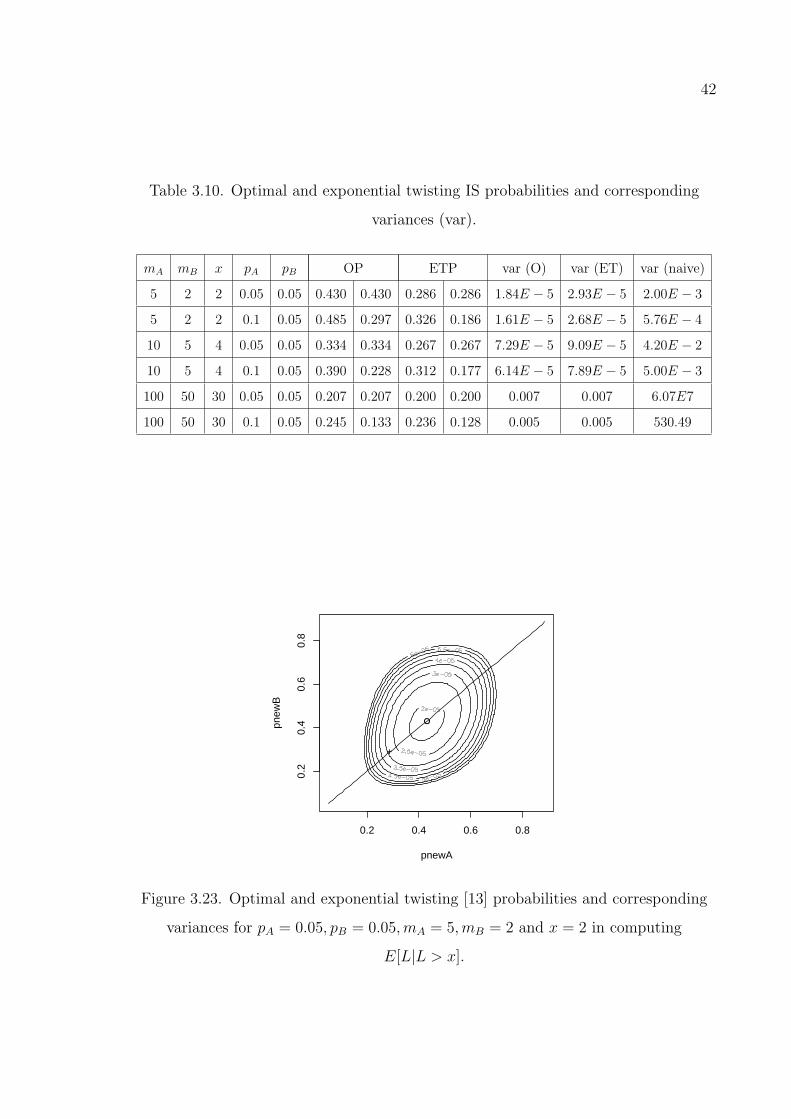
42


variances (var).

mA mB x pA pB OP ETP var (O) var (ET) var (naive)

5 2 2 0.05 0.05 0.430 0.430 0.286 0.286 1.84E − 5 2.93E − 5 2.00E − 3

5 2 2 0.1 0.05 0.485 0.297 0.326 0.186 1.61E − 5 2.68E − 5 5.76E − 4

10 5 4 0.05 0.05 0.334 0.334 0.267 0.267 7.29E − 5 9.09E − 5 4.20E − 2

10 5 4 0.1 0.05 0.390 0.228 0.312 0.177 6.14E − 5 7.89E − 5 5.00E − 3

100 50 30 0.05 0.05 0.207 0.207 0.200 0.200 0.007 0.007 6.07E7

100 50 30 0.1 0.05 0.245 0.133 0.236 0.128 0.005 0.005 530.49

0.2 0.4 0.6 0.8

0.2

0.4

0.6

0.8

pnewA

pnew

B

●

+



E[L|L > x].

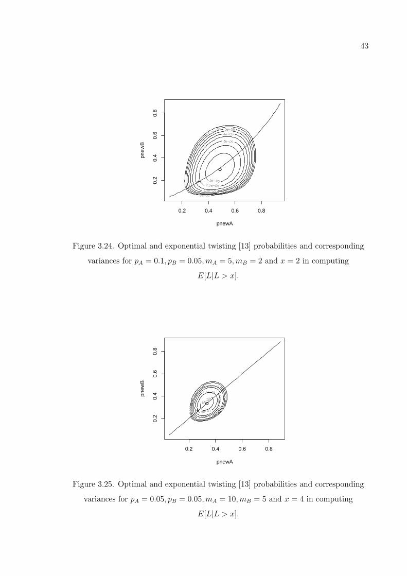
43

0.2 0.4 0.6 0.8

0.2

0.4

0.6

0.8

pnewA

pnew

B

●

+



E[L|L > x].

0.2 0.4 0.6 0.8

0.2

0.4

0.6

0.8

pnewA

pnew

B

●

+



E[L|L > x].

44

0.2 0.4 0.6 0.8

0.2

0.4

0.6

0.8

pnewA

pnew

B

●

+



E[L|L > x].

0.2 0.4 0.6 0.8

0.2

0.4

0.6

0.8

pnewA

pnew

B

●+



E[L|L > x].

45

0.2 0.4 0.6 0.8

0.2

0.4

0.6

0.8

pnewA

pnew

B

●+



E[L|L > x].

are exceptions to this situation in Tables A.1 and A.2. The reason is that for these

tables x = 1. So, the event we simulate is not rare as in Tables A.3 and A.4. And,

sometimes increasing the number of obligors can worsen the asymptotical optimality

since the event was not rare enough and we made it less rare.

The second observation is that when we keep the number of obligors the same

but increase the default probabilities, the performance of exponential twisting gets

worse. However, there is an exception to this. If the default probabilities are the same

then this has an affect on the performance of exponential twisting. Such that percent

difference of variances are not increasing further but decreasing. Under symmetric

default probabilities, exponential twisting works better compared to the non-symmetric

cases.

If we compare the percent differences for x = 1 and x = 5 for both tail loss

probabilities and for expected shortfall, percent differences are always smaller for x = 5.

As we explained above, this is directly related with the rarity of the event we simulate.

46

Finally, some of the exponential twisting probabilities are the same with the naive ones

in Tables A.1 and A.2. As we have explained throughout the chapter, if the expected

value of the loss is greater than or equal to x then the exponential twisting probabilities

are set to the original probabilities.

3.3. Application Example

In this section our aim is to show how our methodology which is used throughout

the chapter could be used to compute optimal probabilities for two small financial

examples.

Our first example is quite similar to the numerical example of [33] where it is

used to demonstrate that expected shortfall is a better risk measure than VaR when

one considers the tail risk of the portfolio. See Table 3.11 for the specific profile of

bonds in the mutual funds. Suppose that we want to invest 100 million dollar to these

mutual funds. We assume that defaults occur totally independently and maturity is 1

year. Moreover, we accept that all the information given in Table 3.11 is constant in

this 1 year duration.

If we use the notation below;

W0 : Initial wealth

W : Wealth at the end of the year 1

X1 : Amount invested in portfolio A

X2 : Amount invested in portfolio B,

then the expected utility (assuming logarithmic utility) of the final wealth will be

E[u(W )] =100∑i=0

(100

i

)0.01i0.99100−i

50∑j=0

(50

j

)0.05j0.9550−j ln(w(i, j))

where

w(i, j) = 1.03X1100− i

100+ 1.05X2

50− j50

+ 1.02(W0 −X1 −X2). (3.7)

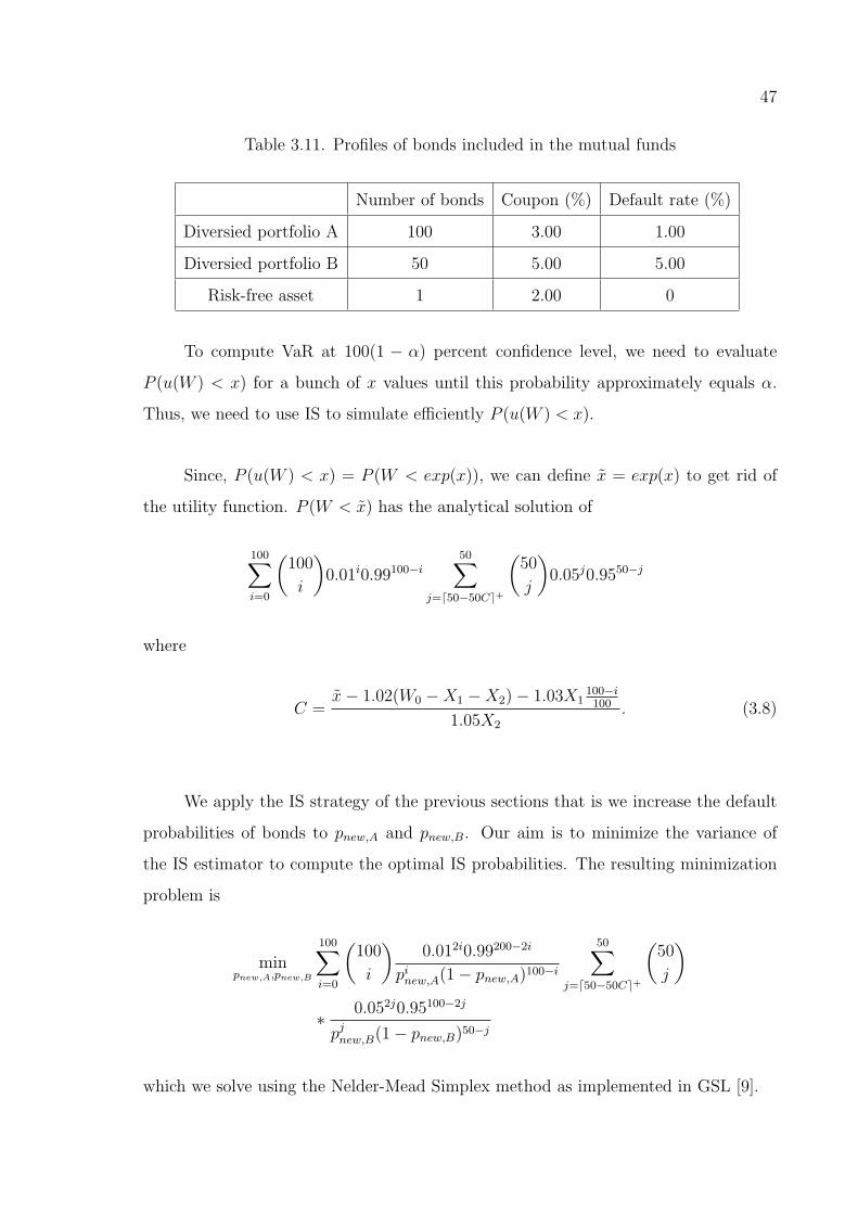
47

Table 3.11. Profiles of bonds included in the mutual funds

Number of bonds Coupon (%) Default rate (%)

Diversied portfolio A 100 3.00 1.00

Diversied portfolio B 50 5.00 5.00

Risk-free asset 1 2.00 0

To compute VaR at 100(1 − α) percent confidence level, we need to evaluate

P (u(W ) < x) for a bunch of x values until this probability approximately equals α.

Thus, we need to use IS to simulate efficiently P (u(W ) < x).

Since, P (u(W ) < x) = P (W < exp(x)), we can define x = exp(x) to get rid of

the utility function. P (W < x) has the analytical solution of

100∑i=0

(100

i

)0.01i0.99100−i

50∑j=d50−50Ce+

(50

j

)0.05j0.9550−j

where

C =x− 1.02(W0 −X1 −X2)− 1.03X1

100−i100

1.05X2

. (3.8)

We apply the IS strategy of the previous sections that is we increase the default

probabilities of bonds to pnew,A and pnew,B. Our aim is to minimize the variance of

the IS estimator to compute the optimal IS probabilities. The resulting minimization

problem is

minpnew,A,pnew,B

100∑i=0

(100

i

)0.012i0.99200−2i

pinew,A(1− pnew,A)100−i

50∑j=d50−50Ce+

(50

j

)

∗ 0.052j0.95100−2j

pjnew,B(1− pnew,B)50−j

which we solve using the Nelder-Mead Simplex method as implemented in GSL [9].

48


variances to compute P (W < x).

x P (W < x) OP ETP var (O) var (ET) var (naive)

100 5.33E − 2 0.026 0.092 0.023 0.085 6.22E − 7 6.56E − 7 5.04E − 6

99 6.47E − 3 0.035 0.111 0.032 0.106 1.39E − 8 1.43E − 8 6.43E − 7

98.5 2.46E − 3 0.039 0.119 0.037 0.115 2.27E − 9 2.30E − 9 2.45E − 7

98.2 9.87E − 4 0.040 0.131 0.040 0.121 4.10E − 10 4.31E − 10 9.86E − 8

98 6.68E − 4 0.041 0.136 0.042 0.124 1.94E − 10 2.07E − 10 6.68E − 8

To compute the exponential twisting probabilities (pnew,A, pnew,B), first of all we

should declare two variables (cA, cB) for the losses. Here, cA = X1(1 + 0.03)/mA and

cB = X2(1+0.05)/mB. Then, remember that exponential twisting uses the strategy; if

E[W ] > x then choose θ such that Eθ[W ] = x otherwise θ = 0 given that pnew,A(θ) =

pAeθcA

pAeθcA+(1−pA)

and pnew,B(θ) = pBeθcB

pBeθcB+(1−pB)

.

For X1 = 60, X2 = 20, we compute optimal and exponential twisting probabilities

for a series of x values in Table 3.12. Note that variances given in this table are for

10, 000 number of replications for all of the methods.

The second problem is to compute E[W |W < x] which has the analytical solution

of

1

P (W < x)

100∑i=0

(100

i

)0.01i0.99100−i

50∑j=d50−50Ce+

(50

j

)0.05j0.9550−jw(i, j)

where w is given in (3.7) and C is given in (3.8).

As we have done in previous sections, the asymptotic variance of our IS estimator

49


variances to compute E[W |W < x].

x E[W |W < x] OP ETP var (O) var (ET) var (naive)

100 99.47 0.026 0.092 0.023 0.085 2.18 2.30 17.58

99 98.51 0.035 0.111 0.032 0.106 3.23 3.33 149.05

98.5 98.12 0.039 0.119 0.037 0.115 3.64 3.69 390.85

98.2 97.77 0.040 0.131 0.040 0.121 4.04 4.25 967.25

98 97.63 0.041 0.136 0.042 0.124 4.15 4.43 1425.60

is

1

nP (W < x)2

[100∑i=0

(100

i

)0.012i0.99200−2i


50∑j=d50−50Ce+

(50

j

)

∗ 0.052j0.95100−2j

pjnew,B(1− pnew,B)50−j(w(i, j))2

−

100∑i=0

(100

i

)0.01i0.99100−i

50∑j=d50−50Ce+

(50

j

)0.05j0.9550−jw(i, j)

2 ]

Thus, the minimization problem for the optimal IS probabilities is

minpnew,A,pnew,B

100∑i=0

(100

i

)0.012i0.99200−2i


50∑j=d50−50Ce+

(50

j

)

∗ 0.052j0.95100−2j

pjnew,B(1− pnew,B)50−j(w(i, j))2

which we solve again using the Nelder-Mead Simplex method as implemented in GSL.

For X1 = 60, X2 = 20, we compute optimal and exponential twisting probabilities

for a series of x values in Table 3.13. Note that, variances given in this table are

for 10, 000 number of replications for all of the methods. Furthermore, we use the

same exponential twisting probabilities computed for simulating P (W < x). To our

knowledge, this is the proposed strategy in related papers for applying exponential

twisting for ES. If we compare the optimal probabilities in Tables 3.12 and 3.13, we

50

see that they are the same indeed. Thus, we see the correctness of this approach by

this small example.

3.3.1. Example 2

Our second numerical example is a portfolio consisting of obligors from two rating

groups, A and B. We have 1000 obligors (mA = mB = 1000) in each group and default

probabilities are 0.005 and 0.02. However, contrary to our first example exposure levels

are not the same in the groups. They have the form given below

cA,j = (d5j/mAe)2, j = 1, ...,mA

cB,j = (d5j/mBe)2, j = 1, ...,mB.

Possible exposures are 1, 4, 9, 16, and 25, with 200 obligors at each level. There

is no easy analytical solution for tail loss probability and expected shortfall in this

case. Our aim is again to compare optimal and exponential twisting probabilities and

corresponding variances but this time we should use simulation to compute them. We

use GSL to solve the 10-dimensional (10 groups of obligors) optimization problem for

optimal IS and the 1-dimensional optimization problem for exponential twisting using

1, 000, 000 replications of the simulations. In exponential twisting, we want to compute

a θ that will change the default probabilities as in (2.4) so that expectation of the losses

under this new measure will be equal to x.

The resultant variances are given in Table 3.14 for P (L > x) and in Table 3.15 for

E[L|L > x]. Note that the given variances are for 10, 000 replications. The numerical

results in this section once again show that exponential twisting probabilities are nearly

the same with optimal ones when the number of obligors is high and the event we

simulate is the rare.

[33] compares VaR and ES in a simple real-world problem. They conclude that

ES should also be used for financial risk management. However, they complain about

51

Table 3.14. Variances for simulating P (L > x) under IS using optimal and

exponential twisting probabilities and naive simulation.

x P (L > x) var (O) var (ET) var (naive)

400 4.33E − 2 4.05E − 7 4.22E − 7 4.13E − 6

450 9.88E − 3 2.93E − 8 3.07E − 8 1.04E − 6

500 1.81E − 3 1.21E − 9 1.27E − 9 1.90E − 7

550 2.67E − 4 3.01E − 11 3.01E − 11 2.00E − 8

Table 3.15. Variances for simulating E[L|L > x] under IS using optimal and

exponential twisting probabilities and naive simulation.

x E[L|L > x] var (O) var (ET) var (naive)

400 433.74 36.83 39.99 410.95

450 479.68 63.61 64.85 2626.26

500 526.49 98.57 99.11 13253.54

550 573.72 138.29 139.96 434281.00

the requirement of increased sample sizes (compared to VaR) when computing ES.

Different to that comment of [33], we have shown that IS can be easily applied to

compute the expected shortfall.

52

4. A NEW ALGORITHM FOR THE NORMAL COPULA

MODEL

In this chapter we propose a new efficient simulation method for computing tail

loss probabilities and conditional expectations in the normal copula framework. We re-

place inner IS (exponential twisting) by inner replications implemented by a geometric

shortcut.

It is important to estimate tail loss probabilities and conditional expectations for

VaR and ES. We first discuss the problem of simulating tail loss probabilities and

conditional expectations for single loss and value at risk values. In Section 4.5 we

consider the problem of simulating tail loss probabilities and conditional expectations

for several loss and value at risk values simultaneously.

4.1. Geometric Shortcut: Independent Obligors

We first consider the case of independent obligors (i.e. set all ajl = 0). This is

useful to clarify how we can improve naive simulation for computing tail probabilities.

The naive algorithm for tail loss probability computation is given in Figure 4.1.


1. generate Yj, j = 1, ...,m, from pj(z);


j=1 cjYj;

2. Return 1n

n∑k=1

1{L(k)>x}.

Figure 4.1. Tail loss probability computation using naive simulation for independent

obligors.

We use the default probabilities to generate default indicators in step 1 of the

algorithm given in Figure 4.1. We can always decrease the variance of P (L > x)

by increasing the number of replications without any variance reduction technique.

53

However, before increasing the number of replications, we should make the simulation

fast so that increasing the number of replications does not change the cost of naive

simulation too much. To accomplish this, observe that we only use the loss values of

replications in the output. Thus, we don’t need to generate each default indicator.

Instead, it is enough to know in which replications defaults occurred for each obligor.

So, for a large number of replications, e.g. n = 1000, and small values of pj it is sensible

to use the geometric distribution to generate the defaults for each obligor. Whenever

we get a default for obligor j, we increase the loss value (L(k)) for that replication by

the loss level of obligor j. That is, we change the direction of the simulation. Instead

of simulating the loss repetition by repetition we simulate the defaults of n repetitions

obligor by obligor. A visualization of this idea is given in Figure 4.2. Algorithm given

in Figure 4.3 contains the details of the “geometric shortcut” idea.

1'st GeometricJump

2'nd GeometricJump

3'rd GeometricJump

r.1r.2r.3

1'st GeometricJump

2'nd GeometricJump

3'rd GeometricJump

Obl. 1 Obl. 2 Obl. m

2'nd GeometricJump

3'rd GeometricJump

r.n

1'st GeometricJump

L(1)

L(2)

L(3)

L(n)

Figure 4.2. Geometric shortcut in generating default indicators

Let’s compute the speed up by comparing the required number of uniform random

numbers in the algorithms given in Figures 4.1 and 4.3 under the assumption that

generating geometric random variate has the same cost as generating uniform random

variates. Obviously 1 + bnpjc is the expected number of uniform random numbers

required for obligor j in the algorithm given in Figure 4.3. Moreover, if we use the

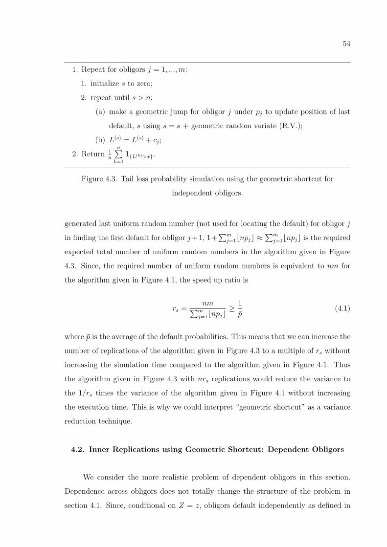
54

1. Repeat for obligors j = 1, ...,m:

1. initialize s to zero;

2. repeat until s > n:

(a) make a geometric jump for obligor j under pj to update position of last

default, s using s = s + geometric random variate (R.V.);

(b) L(s) = L(s) + cj;

2. Return 1n

n∑k=1

1{L(k)>x}.

Figure 4.3. Tail loss probability simulation using the geometric shortcut for

independent obligors.

generated last uniform random number (not used for locating the default) for obligor j

in finding the first default for obligor j+1, 1+∑m

j=1bnpjc ≈∑m

j=1bnpjc is the required

expected total number of uniform random numbers in the algorithm given in Figure

4.3. Since, the required number of uniform random numbers is equivalent to nm for

the algorithm given in Figure 4.1, the speed up ratio is

rs =nm∑m

j=1bnpjc≥ 1

p(4.1)

where p is the average of the default probabilities. This means that we can increase the

number of replications of the algorithm given in Figure 4.3 to a multiple of rs without

increasing the simulation time compared to the algorithm given in Figure 4.1. Thus

the algorithm given in Figure 4.3 with nrs replications would reduce the variance to

the 1/rs times the variance of the algorithm given in Figure 4.1 without increasing

the execution time. This is why we could interpret “geometric shortcut” as a variance

reduction technique.

4.2. Inner Replications using Geometric Shortcut: Dependent Obligors

We consider the more realistic problem of dependent obligors in this section.

Dependence across obligors does not totally change the structure of the problem in

section 4.1. Since, conditional on Z = z, obligors default independently as defined in

55

(2.2).

1. Repeat for replications k = 1, ..., n: /* Outer replications */

1. generate zl ∼ N(0, 1), l = 1, ..., d, independently;

2. calculate pj(z), j = 1, ...,m, as in (2.2) where z = (z1, ..., zd);

3. generate Yj, j = 1, ...,m, from pj(z); /* Inner replications of size 1 */


j=1 cjYj;

2. Return 1n

n∑k=1

1{L(k)>x}.

Figure 4.4. Tail loss probability computation using naive simulation for dependent

obligors.

Let us first give the naive simulation algorithm in Figure 4.4 to better explain

the possible improvement over it. We have to add two steps to the the independent

obligors case of the algorithm given in Figure 4.1: generating common risk factors and

calculating the conditional default probabilities. We would like to make use of the

geometric distribution to generate the default indicators for each obligor. However,

we can not proceed with the same pj values as, for each replication we have different

conditional default probabilities for each obligor. Thus, the only way we can use the

geometric shortcut is by increasing the number of inner replications. As a matter of

fact, it seems sensible to use the conditional default probabilities more than once as

their computation is quite expensive. We give a visualization of our algorithm in Figure

4.5 and the algorithm in Figure 4.6.

In the previous section for independent obligors we have calculated the speed up

ratio in (4.1). If we compute the same ratio, this time comparing the algorithms given

in Figures 4.4 and 4.6, for one outer replication, we get

m∑mj=1bninpj(z)c

≥ m∑mj=1 ninpj(z)

=1

ninpZ≥ 1

nin

⌊1

pZ

⌋

where pZ is the average of the conditional default probabilities for obligors. We don’t

want to be much slower than the naive simulation so this ratio should be greater than

56

1'st GeometricJump

2'nd GeometricJump

3'rd GeometricJump

i.r.1i.r.2i.r.3

Obl. 1 Obl. m

2'nd GeometricJump

3'rd GeometricJump

i.r.nin

1'st GeometricJump

1'st GeometricJump

2'nd GeometricJump

3'rd GeometricJump

i.r.1i.r.2i.r.3

Obl. 1 Obl. m

2'nd GeometricJump

3'rd GeometricJump

1'st GeometricJump

i.r.nin

L(1)

L(2)

L(3)

L(nin)L(nin)

L(1)

L(2)

L(3)

Outer Replication 1 Outer Replication n

Figure 4.5. Inner replications using geometric shortcut in generating default

indicators

1. Thus,

nin ≤⌊

1

pZ

⌋.

Up to now we compare inner replications of the algorithms given in Figures 4.4

and 4.6 (step (3) of the algorithm given in Figure 4.4 and step (4) of the algorithm

given in Figure 4.6). But, nin is also used in step 5 of the algorithm given in Figure

4.6. And, this step should not take much longer than calculating conditional default

probabilities (common step for both algorithms). Therefore, we should select nin such

that nin ≤ m. When we combine both constraints, we get nin = min(b1/pZc,m).

57




3. construct a loss vector L(in) of size nin = min(b1/pZc,m);

4. repeat for obligors j = 1, ...,m; /* Inner replications */

(a) initialize s to zero;

(b) repeat until s > n;

(I) make a geometric jump for obligor j under pj(z) using s = s +

geometric R.V.; ;

(II) L(s)(in) = L

(s)(in) + cj;

5. compute p(k)in = 1

nin

nin∑t=1

1{L(t)(in)

>x} where p(k)in denotes the loss probability of repli-

cation k;

2. Return 1n

n∑k=1

p(k)in .

Figure 4.6. Tail loss probability simulation using inner replications using the

geometric shortcut for dependent obligors.

58

4.3. Integrating IS with Inner Replications using the Geometric Shortcut:

Dependent Obligors

The implementation of inner replications using the geometric shortcut alone is

not sufficient to decrease the variance for highly dependent obligors. Because the main

source of variance is the outer simulation not the inner one for highly dependent oblig-

ors. Thus we need an IS strategy on Z to increase the conditional default probabilities.

It is easy to use a multi-normal IS density with different means (µl) and standard de-

viations (σl) for l = 1, ..., d. However, just shifting the mean vector could be sufficient

for the normal copula framework (see [14]). As mean shift we use the mode of the

zero-variance IS distribution (see Chapter 5).

Finding the mode of the zero-variance IS distribution requires the solution of the

multidimensional optimization problem;

maxzP (L > x|Z = z)e−z

T z/2.

We use the normal approximation for P (L > x|Z) because it is fast and reliable

in computing mean shifts compared to other methods (see Chapter 5). Since, E[L|Z =

z] =∑m

j=1 cjpj(z) and V ar[L|Z = z] =∑m

j=1 c2j [pj(z)− pj(z)2], we can use the normal

approximation:

P (L > x|Z = z) ≈ 1− Φ

(x− E[L|Z = z]√V ar[L|Z = z]

).

Thus, we have to solve the optimization problem

maxz

[1− Φ

(x− E[L|Z = z]√V ar[L|Z = z]

)]e−z

T z/2. (4.2)

After selecting a new mean µ for Z, we combine IS with inner replications using the

59

geometric shortcut. Only two steps of the algorithm given in Figure 4.6 are affected by

this integration. In step (1) of the algorithm given in Figure 4.6, instead of generating

zl from N(0, 1) we generate it from N(µl, 1) where µl is the component of vector µ in

dimension l. And, in step (5), we have to multiply the loss probability of the inner

replication k with the likelihood ratio

wµ = e−µTZ+µTµ/2, (4.3)

which relates the density of the N(0, I) distribution to that of the N(µ, I) distribution

where I is the identity matrix. The full algorithm is given below for the sake of

completeness.




2. calculate wµ as in (4.3);


4. construct a loss vector L(in) of size nin = min(b1/pZc,m);




(I) make a geometric jump for obligor j under pj(z) to update s = s +

R.V.;

(II) L(s)(in) = L

(s)(in) + cj;

6. compute p(k)in = wµ

nin

nin∑t=1

1{L(t)(in)

>x}. where p(k)in stands for the loss probability of

replication k;

3. Return 1n

n∑k=1

p(k)in .

Figure 4.7. Tail loss probability simulation using integration of IS with inner

replications using the geometric shortcut for dependent obligors.

60

4.4. Computing Conditional Expectation of Loss: Dependent Obligors

We described our new methodology for tail loss probability computation. It

is time to explain how the same methodology can be used for the computation of

conditional expectations. We consider only the integration of IS with inner replications

using the geometric shortcut for dependent obligors.

If we assume that P (L ≥ VaRα) > 0, ES can be represented as

r = E[L|L ≥ VaRα] =E[L1{L≥VaRα}

]P (L ≥ VaRα)

.

The naive simulation estimate for this ratio is

rnaive =

∑nk=1 L

(k)1{L(k)≥VaRα}∑nk=1 1{L(k)≥VaRα}

. (4.4)

See the algorithm using this estimate for ES given below.




3. generate Yj, j = 1, ...,m, from pj(z); /* Inner replications of size 1 */


j=1 cjYj;

2. Return rnaive.

Figure 4.8. Naive simulation for computing ES for dependent obligors.

[12] develops IS estimates for computing conditional expectation contributions of

obligors given that large losses occurs for the portfolio. We outline [12] before discussing

our new method for ES but describe the IS estimate of the conditional expectation of

the full portfolio instead of contributions of obligors. If f(z) is our distribution to

generate the z vector and g(z) is the new IS distribution for this purpose, w = f(z)g(z)

61

(equal to (4.3) for our problem) is the likelihood ratio for the generated loss, L. Then

r =E[Lw1{L≥VaRα}

]E[w1{L≥VaRα}]

(4.5)

where E denotes the expectation under the new measure, which means generating z

vector from g(z) instead of f(z) for the simulation estimate.

If L(k) and w(k) denotes the loss and likelihood ratio of the kth replication of a

simulation study in the given order then IS estimator of ES is

rIS =

∑nk=1 L

(k)w(k)1{L(k)≥VaRα}∑nk=1w

(k)1{L(k)≥VaRα}. (4.6)

To compute the precision of (4.6), [12] proposes to use a confidence interval

rIS ± zδ/2σIS√n

(4.7)

where

σIS =

(n∑n

k=1

(L(k)w(k) − rISw(k)

)21{L(k)≥VaRα}(∑n

k=1w(k)1{L(k)≥VaRα}

)2

)1/2

(4.8)

and zδ/2 is the (1 − δ/2) percentile of the standard normal distribution. This confi-

dence interval is given under the conditions; P (L ≥ VaRα) > 0, second moments of

the expectations given in (4.5) are bounded and taking the ratio zero whenever the

denominator is zero in (4.8).

Since, we have IS in our method, we should use a variant of the approach given

above. Inner replications using the geometric shortcut give new loss values in the

number of inner replications per replication. Thus, taking the average of loss values in

an inner replication and then using this value L(k) in (4.6) will be our new estimate for

62

ES. Thus,

rnew =

∑nk=1 L

(k)w(k)1{L(k)≥VaRα}∑nk=1w

(k)1{L(k)≥VaRα}. (4.9)

In the same manner, we can use the confidence interval given in (4.7) by just replacing

L(k) with L(k). See the algorithm given in Figure 4.9.




2. calculate w(k) as in (4.3);


4. construct a loss vector Lin of size nin = min(b1/pZc,m);




(I) make a geometric jump for obligor j under pj(z) to update s = s +

R.V.;

(II) L(s)(in) = L

(s)(in) + cj;

6. calculate L(k) = 1nin

∑nint=1 L

(t)in ;

3. Return rnew.

Figure 4.9. ES simulation using integration of IS with inner replications using the

geometric shortcut for dependent obligors.

4.5. Numerical Results

In this section, we evaluate the performance of our new method for the numerical

examples of [13]. We compare our new approach with naive Monte Carlo simulation

and the two-step IS method of [13] and [12] (both abbreviated as IS in the tables). We

give two different tables for the numerical examples. While, the first table compares

methods according to the size of the half lengths of the confidence intervals for point

estimates of tail loss probabilities, the second table does the same for point estimates

63

of the ES. We also give execution times of the methods for a better comparison.

Probability and half length of the 95 percent confidence interval are abbreviated as

prob. and hl in the tables. In the final column of the tables, we supply the variance

ratio (VR); variance of IS divided by variance of the new method for easy comparison.

See Appendix B.2 for the C codes.

The normal approximation method for computing mean shifts produces very sim-

ilar results with the tail bound approximation given in [13]. Thus, to compare solely

inner IS (exponential twisting) with inner replications using the geometric shortcut, we

use normal approximation to compute the optimal shifts for both methods in the nu-

merical results. Note that, the computation of the θ parameter, for twisting the default

probabilities in [13] is a tedious job. It is an optimization problem and computation

of accurate θ values decreases the variance but increases the execution time. We spent

some time to reach a fast and sufficiently precise version of the Newton method. Our

first implementation was 30 percent slower.

The first example of [13] is a portfolio of m = 1000 obligors in a 10-factor model.

The marginal default probabilities and exposures have the following form:

pj = 0.01(1 + sin(16Πj/m)), j = 1, ...,m;

cj = (d5j/me)2, j = 1, ...,m.

Thus, the marginal default probabilities vary between 0 percent and 2 percent

with a mean of 1 percent, and the possible exposures are 1, 4, 9, 16, and 25, with 200

obligors at each level. These parameters represent a significant departure from an

homogeneous model with constant pj.

For the factor loadings, the ajl are generated independently and uniformly from

the interval (0, 1/√d), d = 10; the upper limit of this interval ensures that the sum of

squared entries a2j1, ..., a

2jd for each obligor does not exceed 1. We simulate the tail loss

probability and expected shortfall for a series of x and VaRα values in Tables 4.1 and

64

4.2. Half lengths of the confidence intervals for the simulations and execution times of

the methods are given in the tables.

Table 4.1. Tail loss probabilities and half lengths (hl) of the confidence intervals for

naive, IS and the new method in the 10-factor model. n = 10, 000. Execution times

(in seconds) are in parentheses.

x prob. (naive) hl (naive) prob. (IS) hl (IS) prob. (new) hl (new) VR

500 3.78 ∗ 10−2(6) 3.73 ∗ 10−3 3.80 ∗ 10−2(15) 1.15 ∗ 10−3 3.81 ∗ 10−3(11) 8.66 ∗ 10−4 1.75

1, 000 9.40 ∗ 10−3(7) 1.89 ∗ 10−3 8.45 ∗ 10−3(16) 2.90 ∗ 10−4 8.55 ∗ 10−3(11) 2.29 ∗ 10−4 1.6

2, 000 9.00 ∗ 10−4(7) 5.88 ∗ 10−4 8.21 ∗ 10−4(16) 2.93 ∗ 10−5 8.54 ∗ 10−4(11) 2.69 ∗ 10−5 1.19

3, 000 1.00 ∗ 10−4(7) 1.96 ∗ 10−4 1.02 ∗ 10−4(16) 3.92 ∗ 10−6 1.07 ∗ 10−4(11) 3.79 ∗ 10−6 1.07

4, 000 - - 1.33 ∗ 10−5(16) 5.53 ∗ 10−7 1.29 ∗ 10−5(11) 5.25 ∗ 10−7 1.10

5, 000 - - 1.36 ∗ 10−6(16) 6.51 ∗ 10−8 1.42 ∗ 10−6(10) 6.07 ∗ 10−8 1.15

Table 4.2. ES values and half lengths (hl) of the confidence intervals using naive, IS

and the new method in the 10-factor model. n = 100, 000. Execution times (in

seconds) are in parentheses.

VaRα ES (naive) hl ES (IS) hl ES (new) hl VR

500 842.7(67) 12.5 841.1(147) 3.0 845.5(109) 2.9 1.07

1, 000 1, 413.8(66) 29.9 1, 419.2(150) 3.9 1, 420.2(106) 3.8 1.05

2, 000 2, 468.7(66) 98.5 2, 478.5(154) 4.3 2, 475.4(103) 4.6 0.87

3, 000 3, 471.9(66) 172.2 3, 476.3(145) 4.4 3, 476.1(101) 4.8 0.84

4, 000 4,744.5(65) 746.3 4, 452.9(153) 4.5 4, 444.4(98) 4.8 0.88

5, 000 - - 5, 403.1(155) 4.5 5, 397.7(97) 4.6 0.96

The next example is a 21-factor model, again with 1, 000 obligors. The marginal

default probabilities fluctuate as in the first example, and the exposures ci increases

from 1 to 100 linearly as i increases from 1 to 1, 000. The matrix of the factor loadings,

A = (ajl, j = 1, ..., 1000, l = 1, ..., 21), has the following block structure:

A =

R∣∣∣∣∣∣∣∣∣F

. . .

F

∣∣∣∣∣∣∣∣∣G...

G

, G =

g

. . .

g

,

65


naive, IS and the new method in the 21-factor model. n = 10, 000. Execution times


x prob. (naive) hl prob. (IS) hl prob. (new) hl VR

2, 500 5.20 ∗ 10−2(8) 4.36 ∗ 10−3 5.09 ∗ 10−2(17) 1.73 ∗ 10−3 5.03 ∗ 10−2(15) 1.57 ∗ 10−3 1.22

10, 000 1.09 ∗ 10−2(8) 2.04 ∗ 10−3 1.11 ∗ 10−2(21) 4.17 ∗ 10−4 1.12 ∗ 10−2(16) 4.02 ∗ 10−4 1.08

20, 000 2.30 ∗ 10−3(8) 9.39 ∗ 10−4 2.71 ∗ 10−3(20) 9.68 ∗ 10−5 2.77 ∗ 10−3(15) 9.74 ∗ 10−5 0.99

30, 000 8.00 ∗ 10−4(8) 5.53 ∗ 10−4 6.26 ∗ 10−4(20) 2.43 ∗ 10−5 6.37 ∗ 10−4(13) 2.47 ∗ 10−5 0.97

40, 000 - - 7.47 ∗ 10−5(21) 3.45 ∗ 10−6 7.36 ∗ 10−5(13) 3.35 ∗ 10−6 1.04

with R a column vector of 1, 000 entries all equal to 0.8; F, a column vector of 100

entries all equal to 0.4; G a 100× 10 matrix, and g, a column vector of 10 entries, all

equal to 0.4. We simulate the tail loss probability and expected shortfall for a series of

x and VaRα values in Tables 4.3 and 4.4.





2, 500 7, 614.7(208) 107.2 7, 584.6(349) 31.2 7, 580.3(307) 31.2 1.0

10, 000 16, 782.9(209) 237.9 16, 798.3(400) 41.5 16, 827.5(311) 41.8 0.99

20, 000 26, 195.7(209) 430.8 26, 395.6(442) 36.4 26, 422.9(302) 36.5 0.99

30, 000 34, 637.9(209) 569.1 34, 831.1(465) 28.4 34, 832.9(296) 28.6 0.99

40, 000 42,379.5(208) 959.0 42, 590.1(477) 16.9 42, 597.5(287) 17.0 0.99

We defined the third numerical example ourselves. It is a 5-factor model with

4800 obligors. Obligors are separated into 6 segments of size 800 each as seen in Table

4.5. Default probabilities, exposure levels and factor loadings are the same in each

segment for the obligors. We again simulate the tail loss probability and expected

shortfall for a series of x and VaRα values in Tables 4.6 and 4.7.

66

Table 4.5. Portfolio composition for the 5-factor model; default probabilities,

exposure levels and factor loadings for six segments.

Segment Obligor j pj cj aj,1 aj,2 aj,3 aj,4 aj,5

1A 1− 800 0.01 20 0.7 0.5 0.1

1B 801− 1600 0.02 10 0.7 0.5 0.1

2A 1601− 2400 0.02 10 0.7 0.2 0.4

2B 2401− 3200 0.04 5 0.7 0.2 0.4

3A 3201− 4000 0.03 5 0.7 0.4 0.5

3B 4001− 4800 0.05 1 0.7 0.4 0.5


naive, IS and the new method in the 5-factor model. n = 10, 000. Execution times (in



5, 000 4.66 ∗ 10−2(25) 4.13 ∗ 10−3 4.55 ∗ 10−2(52) 1.52 ∗ 10−3 4.55 ∗ 10−3(37) 1.46 ∗ 10−3 1.09

10, 000 2.02 ∗ 10−2(24) 2.76 ∗ 10−3 1.94 ∗ 10−2(53) 6.96 ∗ 10−4 1.81 ∗ 10−2(37) 5.97 ∗ 10−4 1.36

15, 000 8.00 ∗ 10−3(24) 1.75 ∗ 10−3 8.50 ∗ 10−3(54) 2.95 ∗ 10−4 8.36 ∗ 10−3(37) 2.84 ∗ 10−4 1.08

20, 000 5.30 ∗ 10−3(24) 1.42 ∗ 10−3 3.87 ∗ 10−3(57) 1.36 ∗ 10−4 4.03 ∗ 10−3(36) 1.39 ∗ 10−4 0.95

25, 000 2.40 ∗ 10−3(24) 9.59 ∗ 10−4 1.83 ∗ 10−3(57) 6.69 ∗ 10−5 1.81 ∗ 10−3(37) 6.60 ∗ 10−5 1.03

30, 000 1.10 ∗ 10−3(24) 6.50 ∗ 10−4 7.80 ∗ 10−4(59) 3.05 ∗ 10−5 8.13 ∗ 10−4(36) 3.11 ∗ 10−5 0.96





5, 000 10, 619.2(239) 169.8 10, 730.3(500) 52.4 10, 742.4(368) 55.0 0.91

10, 000 16, 167.4(240) 265.8 16, 295.9(517) 57.3 16, 225.6(367) 57.7 0.98

15, 000 21, 164.6(241) 358.1 21, 307.0(534) 56.4 21, 279.0(367) 56.2 1.00

20, 000 26, 100.9(239) 512.4 25, 836.0(543) 50.8 25, 784.9(365) 51.1 0.99

25, 000 29,989.0(242) 493.5 29, 989.7(559) 43.4 29, 959.6(367) 43.1 1.01

30, 000 33, 661, 6(241) 601.7 33, 748.1(573) 33.4 33, 764.4(368) 34.0 0.96

67

We did some numerical experiments to see how Tables 4.1−4.4 and 4.6−4.7 are

affected if we change the number of inner replications in the new method. They clearly

showed that the main source of variation in the simulation is the outer simulation. We

have arrived at this conclusion since increasing the number of inner replications does

not reduce the variance any more. Our choice for the number of inner replications used

in the algorithms is obviously a good approximation for the optimal number of inner

replications. Thus, we can report that both of the methods as the inner simulations

(inner replications using the geometric shortcut or exponential twisting) most of the

time reduce the variance as much as they could. But, we can add some comments; the

new method performs better when calculating larger loss probabilities for out of tail

cases and the new method is approximately one and a half times faster than IS in all

cases.

4.5.1. Simultaneous Simulations

We separately simulate tail loss probabilities (ES) for all x (VaRα) in producing

Tables 4.1 and 4.3 (4.2 and 4.4). However, in practice people are interested in the

tail loss probability distribution to assess VaR. In the same manner, we want to see

how expected shortfall changes with respect to VaRα. Thus, it is of greatest practical

importance to compute tail loss probabilities and ES for a wide range of x and VaRα

values in a single simulation. So, as the next step we compare these methods in

achieving loss probabilities (ES) simultaneously over a wide range of x (VaRα) values.

IS strategy of [13] ( [12]) fixes optimal mean shift and twisted default probabilities

on x (VaRα). This makes a single simulation of IS at more than one point difficult.

But, in section 6 of [13] it is suggested to use the IS distribution computed at the

smallest loss level for all values we need. Thus, in Table 4.8 (4.9), we apply the IS

distribution computed at x = 500 (VaRα = 500) for the rest of the x (VaRα) for

IS. Contrary to IS of [13] ( [12]), inner replications using the geometric shortcut do

not have any parameter that is related to x (VaRα). This means that there is no

problem to simultaneously apply the geometric shortcut for a wide range of x values

(VaRα). However, the new method is an integration of outer IS and the geometric

68

shortcut. Thus, we should change the implementation of outer IS to make the new

method simultaneously applicable. One simple way could be first of all computing

optimal mean shifts for the minimum and maximum x values (VaRα) then using a

density mixture of the normal distributions having means of these shifts and variances

1 to get optimal mean shifts for simulations. Similarly, instead of sampling from this

density mixture, we can use a normal distribution having the mean and variance of

this density mixture to get samples for the simulation. In Tables 4.8 and 4.9, we use

that normal distribution having the mean and variance of the density mixture of equal

weights as (outer) IS-density.

Combining outer IS described above and the geometric shortcut for inner repli-

cations performs much better than IS applied by [13] as can be seen from Tables 4.8

and 4.9. Only for the smallest x it is a little bit worse than IS as by the design of

outer IS the suggestion of [13] is best for the minimal x value and our normal mixture

approach is worse for small x values. Note that the improvement of our method comes

both from the usage of outer IS with a suitable larger variance and from the usage of

the geometric shortcut which works very well for all x-values considered. Numerical

results for the second example are similar to Tables 4.8 and 4.9, so we do not include

them here. Also note that our new method is about 30 percent and 50 percent faster.

Thus the actual gain is 30 percent and 50 percent higher than the Variance Reduction

factors given in Tables 4.8 and 4.9.

To visiualize what we have observed in Tables 4.8 and 4.9, we have drawn Figures

4.10 and 4.11. Simulations are based on 1, 000 and 10, 000 replications in the given

order for the figures. In each case, the three curves show the sample mean (the center

line) and a 95 percent confidence interval (the two outer lines) computed separately at

each point. Note that, while solid lines refer to sample mean and confidence interval

of the new method, dashed lines refer to sample mean and confidence interval of IS.

69

Table 4.8. Tail loss probabilities and half lengths (hl) of the confidence intervals in a

single simulation using naive, IS and the new method in the 10-factor model.

n = 10, 000. Execution times for the methods are 7, 16 and 12 seconds in the given

order.


500 3.90 ∗ 10−2 3.79 ∗ 10−3 3.90 ∗ 10−2 1.18 ∗ 10−3 3.97 ∗ 10−2 1.73 ∗ 10−3 0.47

1, 000 8.00 ∗ 10−3 1.75 ∗ 10−3 8.35 ∗ 10−3 3.16 ∗ 10−4 8.69 ∗ 10−3 3.09 ∗ 10−4 1.05

1, 500 2.80 ∗ 10−3 1.03 ∗ 10−3 2.42 ∗ 10−3 1.17 ∗ 10−4 2.60 ∗ 10−3 8.73 ∗ 10−5 1.79

2, 000 1.20 ∗ 10−3 6.80 ∗ 10−4 8.29 ∗ 10−4 3.76 ∗ 10−5 8.57 ∗ 10−4 2.99 ∗ 10−5 1.58

2, 500 2.00 ∗ 10−4 2.77 ∗ 10−4 2.84 ∗ 10−4 2.24 ∗ 10−5 3.00 ∗ 10−4 1.12 ∗ 10−5 3.99

3, 000 2.00 ∗ 10−4 2.77 ∗ 10−4 9.86 ∗ 10−5 1.01 ∗ 10−5 1.06 ∗ 10−4 4.46 ∗ 10−6 5.12

3, 500 − − 3.92 ∗ 10−5 5.00 ∗ 10−6 3.65 ∗ 10−5 1.73 ∗ 10−6 8.26

4, 000 − − 1.43 ∗ 10−5 2.40 ∗ 10−6 1.22 ∗ 10−5 6.80 ∗ 10−7 12.5

4, 500 − − 4.51 ∗ 10−6 1.11 ∗ 10−6 4.32 ∗ 10−6 2.73 ∗ 10−7 16.39

5, 000 − − 1.08 ∗ 10−6 4.17 ∗ 10−7 1.39 ∗ 10−6 1.02 ∗ 10−7 16.74

Table 4.9. ES values and half lengths (hl) of the confidence intervals in a single

simulation using naive, IS and the new method in the 10-factor model. n = 100, 000.

Execution times for the methods are 66, 151 and 104 seconds in the given order.


500 839.8 12.3 840.8 3.0 840.6 4.5 0.44

1, 000 1, 440.4 32.9 1, 420.9 4.2 1, 419.2 4.5 0.87

1, 500 1, 914.0 54.4 1, 960.4 5.5 1, 961.2 4.7 1.37

2, 000 2, 429.4 86.7 2, 473.8 7.1 2, 477.7 4.9 2.10

2, 500 3, 135.1 196.8 2, 977.9 9.0 2, 978.7 5.2 3.00

3, 000 3, 602.4 267.7 3, 470.6 11.5 3, 477.3 5.5 4.37

3, 500 4, 081.5 244.6 3, 967.7 14.7 3, 963.8 5.9 6.21

4, 000 4, 473.5 268.2 4, 449.5 19.1 4, 447.6 6.4 8.91

4, 500 − − 4, 918.4 24.3 4, 4925.3 6.9 12.40

5, 000 − − 5, 407.4 32.0 5, 396.5 7.6 17.73

70

1000 2000 3000 4000 5000

1e−

061e

−05

1e−

041e

−03

1e−

02

Loss level

Tai

l pro

babi

lity

new

IS

Figure 4.10. Comparison of new method with IS in estimating tail loss probabilities

in the 10-factor model using 1, 000 replications.

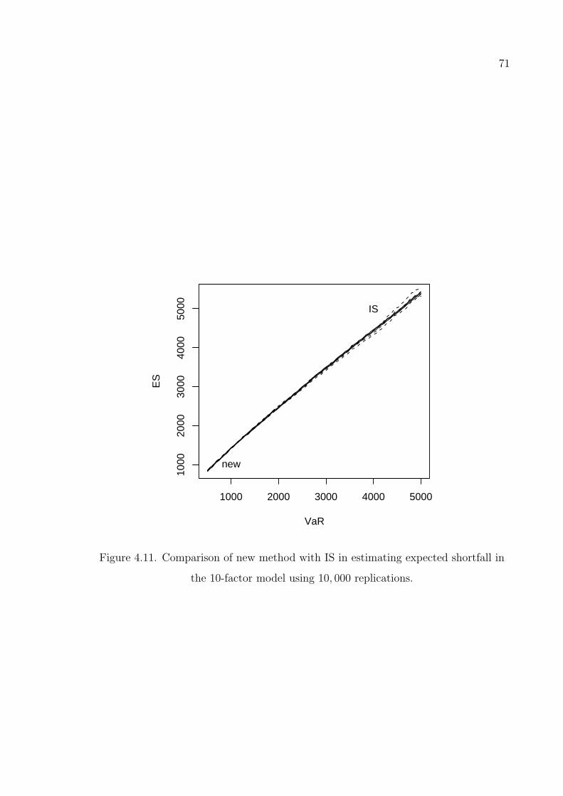
71

1000 2000 3000 4000 5000

1000

2000

3000

4000

5000

VaR

ES

new

IS

Figure 4.11. Comparison of new method with IS in estimating expected shortfall in

the 10-factor model using 10, 000 replications.

72

4.6. Conclusion

We developed a new method for simulating tail loss probabilities and ES for a

standard credit risk portfolio in this Chapter. The new method is an integration of

IS with inner replications using geometric shortcut for dependent obligors in a normal

copula framework. Numerical results show that our new method is much better than

naive simulation for computing tail loss probabilities and ES at a single x and VaRα

value. Furthermore, it is clearly better than two-step IS ( [12,13]) in a single simulation

to compute tail loss probabilities and ES at multiple x and VaRα values.

73

5. COMPARISON OF MEAN SHIFTS FOR IS

For the “normal copula” credit risk model inner importance sampling strategies

such as exponential twisting or inner replications of geometric shortcut proposed in

Chapter 4 are not enough for reducing the variance for highly dependent obligors.

Since, large losses occur primarily because of large outcomes of systematic risk fac-

tors in the normal copula framework. One of the classical methods to use as additional

(outer) importance sampling strategy is to shift the mean of the systematic risk factors.

There are many different approaches that use mean shift optimization heuristics (or

approximations) in the literature. See [7] for a summary and comparison of the three.

Although, these methods often work, [7] reports that some of the mean shifting meth-

ods are performing not better than naive Monte Carlo simulation for middium-sized

portfolios. We consider approximate homogenous portfolios only, since [16] reports

that for a multifactor heterogeneous model the use of a mixture of IS distributions,

each associated with a different shift of mean is required.

In this chapter we first of all explain three different approaches, tail bound ap-

proximation used in [13], normal approximation used in Chapter 4 and homogenous

portfolio approximation of [25]. The first two methods rely on the approximation (pro-

posed by [14]) that finds the optimal mean shift as the mode of the zero-variance IS

distribution whereas the last one uses homogenous portfolio approximation. Then we

assess the performance of these three approximations in the numerical examples of

Chapter 4.

5.1. Mode of Zero-Variance IS Distribution

P (L > x) is the integration of P (L > x|Z) under the distribution of Z. We are

willing to choose a new IS distribution for Z that reduces the variance of Monte Carlo

simulation for this integration. It is well-known that the zero-variance IS distribution

is a normalization of P (L > x|Z = z)e−zT z/2 where e−z

T z/2 is the probability density

of Z = z. However, the normalization constant is P (L > x), we are looking for.

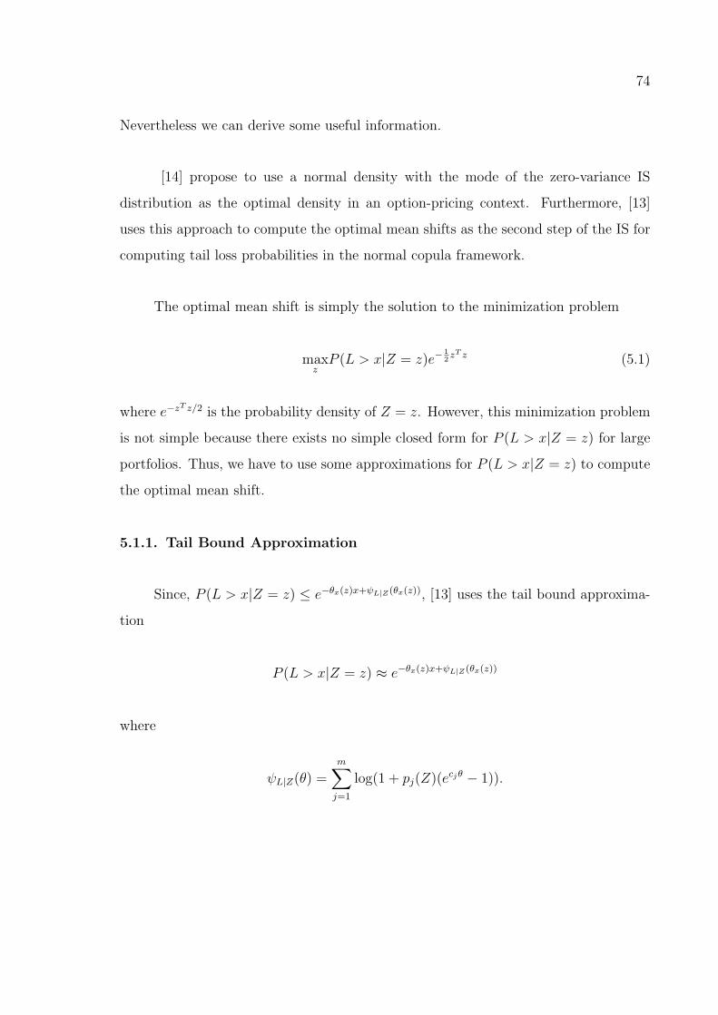
74

Nevertheless we can derive some useful information.

[14] propose to use a normal density with the mode of the zero-variance IS

distribution as the optimal density in an option-pricing context. Furthermore, [13]

uses this approach to compute the optimal mean shifts as the second step of the IS for

computing tail loss probabilities in the normal copula framework.

The optimal mean shift is simply the solution to the minimization problem

maxzP (L > x|Z = z)e−

12zT z (5.1)

where e−zT z/2 is the probability density of Z = z. However, this minimization problem

is not simple because there exists no simple closed form for P (L > x|Z = z) for large

portfolios. Thus, we have to use some approximations for P (L > x|Z = z) to compute

the optimal mean shift.

5.1.1. Tail Bound Approximation

Since, P (L > x|Z = z) ≤ e−θx(z)x+ψL|Z(θx(z)), [13] uses the tail bound approxima-

tion

P (L > x|Z = z) ≈ e−θx(z)x+ψL|Z(θx(z))

where

ψL|Z(θ) =m∑j=1

log(1 + pj(Z)(ecjθ − 1)).

75

5.1.2. Normal Approximation

We compute the conditional expectation and variance of the loss, E[L|Z = z] =∑mj=1 cjpj(z) and V ar[L|Z = z] =

∑mj=1 c

2j [pj(z)− pj(z)2] that we can use the normal

approximation:

P (L > x|Z = z) ≈ 1− Φ

(x− E[L|Z = z]√V ar[L|Z = z]

).

After approximating P (L > x|Z = z) using tail bound or normal approximation,

we solve the d-dimensional optimization problem in (5.1). We use the Nelder-Mead

Simplex method as implemented in GSL to solve the optimization problem.

5.2. Homogenous Portfolio Approximation

[25] proposes an IS strategy that computes an optimal mean shift using homoge-

nous portfolio approximation to calculate expected shortfall for credit portfolios. [25]

approximates the whole portfolio by a homogenous one in which all obligors default

with the same probability p and have the same exposure level c;

p =

∑mj=1 pjcj∑mj=1 cj

, c =

∑mj=1 cj

m.

Moreover, different to the latent variable structure in (2.1) all obligors have the same

factor loadings in the latent variables;

Xj = a0εj + a1Z1 + ..+ adZd, , j = 1, ...,m

where

(a1, ..., ad) =Ψ

swith Ψ = (Ψ1, ...,Ψm) =

m∑j=1

gj(aj1, ..., ajd)

76

and gj = pjcj. The scaling factor s is found by the equation

s2 =1

1− a20

d∑k=1

d∑l=1

ΨkΨlCov(Zk, Zl)

where

1− a20 =

∑dk=1

∑dl=1 ΨkΨlCov(Zk, Zl)−

∑mj=1 g

2j (1− a2

j0)(∑mj=1 gj

)2

−∑m

j=1 g2j

.

Please note that Cov(Zk, Zl) = 1 if k = l otherwise 0 for the credit portfolio model

used in [13] and Chapter 4.

The computation of scaling factor s is based on the idea that the weighted sum of

the latent variables’ covariances in the original and the homogeneous portfolio should

be equal. Thus, following equation holds

m∑i

m∑j

gigjCov(Xi, Xj) =m∑i

m∑j

gigjCov(Xi, Xj).

After evaluating the equivalent homogeneous portfolio, [25] considers the loss

function for the infinite homogeneous portfolio;

L∞d (Z1, ..., Zd) = cΦ(Φ−1(p) +

∑dl=1 alZl

a0

).

The IS estimator that shifts the mean of vector Z as µ = (µ1, ..., µd) is

L∞d 1{L∞d >c∞}N0,1

Nµ,1

for the expected shortfall of the infinite homogeneous portfolio for a given probability

level 100(1−α) percent. Please note that c∞ is the 100(1−α) percent quantile of L∞d .

77

[25] computes µ in two steps. In the first step they decrease the dimension of

the problem to one (only one systematic risk factor) and compute the optimal mean

shift for this case. Then, in the second step, they lift the optimal mean shift computed

in the first step to dimension d.

For the first step, the optimization problem is to find µ(1) that minimizes

∫ ∞Φ−1(1−α)

(L∞1 N0,1)2

Nµ(1),1

dx (5.2)

where

L∞1 = cΦ

(Φ−1(p) +

√1− a2

0x

a0

).

After computing µ(1), [25] uses the following equation

µk =µ(1)

∑dl=1Cov(Zk, Zl)al√

1− a20

, , k = 1, ..., d

to compute the optimal mean shift vector. For more details and proofs see [24].

To summarize, homogenous portfolio approximation of [25] has the advantage of

requiring a one-dimensional optimization problem instead of d-dimensional one. On

the other hand, it includes the evaluation of the numerical integration given in (5.2).

5.3. Numerical Results

In this section, we evaluate the performance of the optimal mean shift algorithms

given in the previous sections for the numerical examples of Chapter 4. Since, our

new methodology proposed in Chapter 4 has an outer IS strategy like the two-step

IS methodology of [13] and variances computed are approximately the same for single

loss values, we can use both of the methods for assessing the performance of outer

IS methodologies. We choose the two-step IS methodology of [13] because it is a well

78

Table 5.1. Half lengths (hl) of the confidence intervals for using tail bound

approximation (TBA), normal approximation (NA) and homogenous approximation

(HA) for the optimal mean shift as outer IS and exponential twisting as inner IS in

the 10-factor model to compute tail loss probabilities. n = 10, 000. Execution times


x prob. hl (TBA) hl (NA) hl (HA)

500 3.87 ∗ 10−2 1.14 ∗ 10−3(17) 1.14 ∗ 10−3(12) 1.19 ∗ 10−3(11)

1, 000 8.67 ∗ 10−3 2.99 ∗ 10−4(16) 2.95 ∗ 10−4(13) 2.99 ∗ 10−4(11)

2, 000 8.43 ∗ 10−4 2.98 ∗ 10−5(15) 2.93 ∗ 10−5(12) 2.99 ∗ 10−5(12)

3, 000 1.08 ∗ 10−4 4.14 ∗ 10−6(17) 3.95 ∗ 10−6(11) 4.10 ∗ 10−6(12)

4, 000 1.32 ∗ 10−5 5.51 ∗ 10−7(17) 5.38 ∗ 10−7(12) 5.52 ∗ 10−7(12)

known method and many could be interested in the results of this comparison. [7] omits

the exponential twisting part of [13] in their comparison of the methods. We include

it to compare the mean shifts for a good simulation method. See Appendix B.3 for the

C codes.

Half lengths (hl) of the confidence intervals for using tail bound approximation

(TBA), normal approximation (NA) and homogenous approximation (HA) for the op-

timal mean shift as outer IS and exponential twisting as inner IS in the 10-factor model

are given in Table 5.1 (to compute tail loss probabilities) and 5.2 (to compute expected

shortfalls). If we compare the half lengths of the confidence intervals, normal approx-

imation is most of the time better than the other two methods. On the other hand,

the fastest one is the homogenous approximation. As we have only slight differences

between the half lengths of the confidence intervals and execution times of the meth-

ods, we can definitely use all three methods for finding the mean shift of outer IS in

the 10-factor model.

Half lengths of the confidence intervals for using tail bound approximation, nor-

mal approximation and homogenous approximation for the optimal mean shift as outer

IS and exponential twisting as inner IS in the 21-factor model are given in Table 5.3

79




the 10-factor model to compute expected shortfalls. n = 100, 000. Execution times


VaRα ES hl (TBA) hl (NA) hl (HA)

500 842.1 2.99(126) 2.99(113) 2.99(108)

1, 000 1, 419.8 3.90(131) 3.91(121) 3.89(114)

2, 000 2, 478.0 4.30(127) 4.25(120) 4.28(120)

3, 000 3, 480.2 4.48(121) 4.48(114) 4.49(110)

4, 000 4, 447.2 4.47(126) 4.50(117) 4.47(117)

(to compute tail loss probabilities) and 5.4 (to compute expected shortfalls). If we

compare the methods according to their half length of the confidence intervals and

execution times, homogeneous approximation is always better than the other two in

the 21-factor model but the differences are small.

Half lengths of the confidence intervals for using tail bound approximation, nor-

mal approximation and homogenous approximation for the optimal mean shift as outer

IS and exponential twisting as inner IS in the 5-factor model are given in Table 5.3

(to compute tail loss probabilities) and 5.4 (to compute expected shortfalls). If we

solely look at the half length of the confidence intervals, homogeneous approximation

is definitely the worst in the 21-factor model. And, normal approximation is generally

slightly better than tail bound approximation. If we compare the execution times,

homogenous approximation is fastest as in the previous models and tail bound approx-

imation is slowest.

Summarizing we evaluate the performance of three mean shift optimization ap-

proximations: tail bound approximation, normal approximation and homogenous ap-

proximation. Note that, the calculated mean shifts are different to each other for the

methods discussed in this section as reported in [13]. For different models, we arrived

80




the 21-factor model to compute tail loss probabilities. n = 10, 000. Execution times



2, 500 4.96 ∗ 10−2 1.62 ∗ 10−3(25) 1.69 ∗ 10−3(14) 1.57 ∗ 10−3(11)

10, 000 1.16 ∗ 10−2 4.10 ∗ 10−4(27) 4.23 ∗ 10−4(16) 3.62 ∗ 10−4(13)

20, 000 2.69 ∗ 10−3 9.69 ∗ 10−5(26) 9.66 ∗ 10−5(17) 9.65 ∗ 10−5(13)

30, 000 6.29 ∗ 10−4 2.51 ∗ 10−5(37) 2.43 ∗ 10−5(17) 2.36 ∗ 10−5(13)

40, 000 7.59 ∗ 10−5 3.48 ∗ 10−6(27) 3.37 ∗ 10−6(16) 3.20 ∗ 10−6(14)




the 21-factor model to compute expected shortfalls. n = 100, 000. Execution times



2, 500 7, 597.3 49.31(125) 49.30(113) 48.73(111)

10, 000 16, 816.3 65.74(140) 65.51(129) 59.95(123)

20, 000 26, 360.4 56.63(150) 57.43(139) 56.45(127)

30, 000 34, 840.7 45.67(168) 44.74(145) 43.75(131)

40, 000 42, 587.9 27.05(160) 26.57(148) 26.05(131)

81




the 5-factor model to compute tail loss probabilities. n = 10, 000. Execution times (in



5, 000 4.64 ∗ 10−2 1.53 ∗ 10−3(55) 1.53 ∗ 10−3(52) 1.55 ∗ 10−3(46)

10, 000 1.82 ∗ 10−2 6.24 ∗ 10−4(56) 6.53 ∗ 10−4(54) 6.34 ∗ 10−4(51)

15, 000 8.29 ∗ 10−3 2.82 ∗ 10−4(58) 2.79 ∗ 10−4(55) 3.20 ∗ 10−4(51)

20, 000 3.91 ∗ 10−3 1.38 ∗ 10−4(61) 1.34 ∗ 10−4(55) 1.67 ∗ 10−4(53)

25, 000 1.88 ∗ 10−3 6.83 ∗ 10−5(60) 6.67 ∗ 10−5(57) 8.27 ∗ 10−5(53)

30, 000 7.71 ∗ 10−4 3.03 ∗ 10−5(67) 3.00 ∗ 10−5(58) 3.47 ∗ 10−5(55)




the 5-factor model to compute expected shortfalls. n = 100, 000. Execution times (in



5, 000 10, 729.5 52.76(513) 53.18(503) 53.38(457)

10, 000 16, 366.8 57.41(539) 56.28(534) 56.74(486)

15, 000 21, 296.4 56.39(540) 56.73(532) 61.05(504)

20, 000 25, 856.6 51.27(553) 50.50(544) 60.78(515)

25, 000 29, 948.1 43.36(565) 43.27(554) 49.38(526)

30, 000 33, 747.6 33.46(582) 33.48(569) 38.00(535)

82

at different conclusions. Half lengths of the confidence intervals are very similar for all

of the approximations. Also, the speed of the approximations are quite similar when

number of factors are large. However, tail bound approximation is slowest for a small

number of factors. Moreover, normal approximation (being simplest) or homogenous

approximation would be our choice when using one of these approximations. Since,

both are fast, reliable and outperform tail bound approximation.

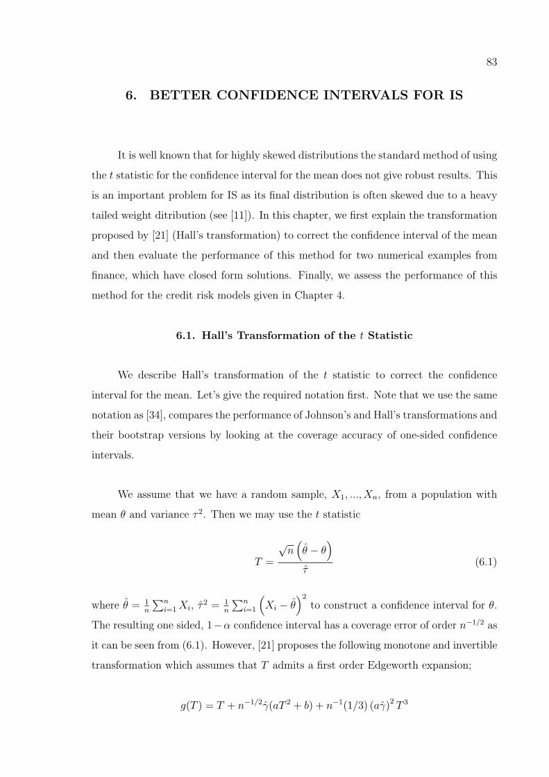
83

6. BETTER CONFIDENCE INTERVALS FOR IS

It is well known that for highly skewed distributions the standard method of using

the t statistic for the confidence interval for the mean does not give robust results. This

is an important problem for IS as its final distribution is often skewed due to a heavy

tailed weight ditribution (see [11]). In this chapter, we first explain the transformation

proposed by [21] (Hall’s transformation) to correct the confidence interval of the mean

and then evaluate the performance of this method for two numerical examples from

finance, which have closed form solutions. Finally, we assess the performance of this

method for the credit risk models given in Chapter 4.

6.1. Hall’s Transformation of the t Statistic

We describe Hall’s transformation of the t statistic to correct the confidence

interval for the mean. Let’s give the required notation first. Note that we use the same

notation as [34], compares the performance of Johnson’s and Hall’s transformations and

their bootstrap versions by looking at the coverage accuracy of one-sided confidence

intervals.

We assume that we have a random sample, X1, ..., Xn, from a population with

mean θ and variance τ 2. Then we may use the t statistic

T =

√n(θ − θ

)τ

(6.1)

where θ = 1n

∑ni=1Xi, τ

2 = 1n

∑ni=1

(Xi − θ

)2

to construct a confidence interval for θ.

The resulting one sided, 1−α confidence interval has a coverage error of order n−1/2 as

it can be seen from (6.1). However, [21] proposes the following monotone and invertible

transformation which assumes that T admits a first order Edgeworth expansion;

g(T ) = T + n−1/2γ(aT 2 + b) + n−1(1/3) (aγ)2 T 3

84

where γ = 1n

∑ni=1

(Xi − θ

)3

/τ 3, a = 1/3, b = 1/6. This transformation has a unique

inverse

T = g−1(x) = n1/2(aγ)−1[(1 + 3aγ(n−1/2x− n−1bγ))1/3 − 1

].

Using this transformation, [21] gives the upper and lower endpoint with confidence

1 − α: (−∞, θ − n−1/2τ g−1(zα)) and (θ − n−1/2τ g−1(z1−α),∞). It can be shown that

for the upper and lower endpoints 1 − α the coverage error converges with speed n−1

instead of n−1/2.

6.2. TWO EXAMPLES

In this section we want to assess the performance of Hall’s transformation com-

pared to the standard t statistics. We consider one-sided coverage accuracies as the

measure of evaluation as [21] and [34]. To be able to simulate exact coverage levels we

choose examples for which analytical solutions are available.

To give the coverage accuracies, we use 10, 000 samples in these examples. We

take the average of the 10, 000 bernoulli trials indicating whether the exact value of

the mean is in the calculated confidence intervals to estimate the coverage accuracies.

Thus, we can expect to have a natural variance on the coverage levels. It is easy to see

that the 99 percent acceptance region for the 95 percent one-sided coverage levels are

0.944 and 0.956. See Appendix B.4 for the C codes

6.2.1. Example 1

We want to compute the following probability

P

(L =

∑di=1 Zi√d

> x

)(6.2)

85

where Zi’s are iid standard normal variates. We are applying an IS strategy such that

new Zi’s are distributed normally with mean µi and standard deviation σi. For the one

dimensional case, we show that if we choose a mean shift (µ) such that the expected

value of L is x then this is an asymptotically optimal mean shift in Appendix A.2.

Thus, we choose µi = x/√d so that the expected value of L is x.

We give the achieved coverage levels for 95 percent upper and lower endpoint

confidence intervals for a series of σi, d and n values in Table 6.1. We observe that Hall’s

confidence interval works better than standard t statistic when n is small. Although,

increasing the dimension of the problem decreases the quality of the confidence level of

both methods except for the case with σi = 1.0, Hall’s transformation produces better

confidence intervals than ordinary t statistic.

6.2.2. Example 2

The maturity of the Asian option is 0.2 (years) and control points are 0.12, 0.14,

0.16, 0.18 and 0.2. We choose a geometric average Asian option to price since we have

a closed form solution for it and the price of it is quite close to an arithmetic average

Asian option.

We use IS to decrease the variance of the simulation. To compute the optimal

IS parameters, we use the Nelder-Mead Simplex method as implemented in GSL. We

use n = 10, 000, 000 for the optimization. Achieved coverage levels for 95 percent

upper and lower endpoint confidence intervals are given in Table 6.2 for S0 = 100 and

r = 0.09. Note that, we use 10, 000 simulated samples to compute the coverage levels.

It is easy to see from Table 6.2, there is no statistical evidence showing Hall’s

method is better than the standard t statistic for small values of the strike price (K).

However, as the strike price increases, Hall’s confidence interval clearly works better

than the standard t statistic.

86


confidence intervals (x = 2)

Upper Endpoint Lower Endpoint

σ d n Ordinary t Hall Ordinary t Hall

0.9

101000 0.935 0.946 0.959 0.948

10000 0.950 0.954 0.953 0.951

201000 0.925 0.942 0.968 0.950

10000 0.935 0.943 0.956 0.948

501000 0.897 0.929 0.980 0.954

10000 0.9257 0.942 0.969 0.950

1.0

101000 0.945 0.952 0.957 0.952

10000 0.947 0.948 0.953 0.951

201000 0.945 0.950 0.956 0.952

10000 0.950 0.951 0.954 0.953

501000 0.946 0.953 0.956 0.951

10000 0.946 0.948 0.954 0.952

1.1

101000 0.943 0.952 0.955 0.948

10000 0.948 0.951 0.955 0.953

201000 0.939 0.950 0.957 0.948

10000 0.943 0.946 0.954 0.952

501000 0.929 0.949 0.966 0.950

10000 0.942 0.949 0.960 0.954

87


confidence intervals (S0 = 100, r = 0.09).

optimal IS Upper Endpoint Lower Endpoint

volatility K µ σ n Ordinary t Hall Ordinary t Hall

0.1

90 0.108 1.0011000 0.955 0.954 0.953 0.954

10000 0.951 0.951 0.949 0.949

100 0.288 1.0351000 0.947 0.950 0.955 0.953

10000 0.947 0.948 0.952 0.952

105 0.477 1.1081000 0.946 0.953 0.958 0.951

10000 0.945 0.948 0.954 0.951

110 0.753 1.2831000 0.927 0.949 0.964 0.949

10000 0.944 0.951 0.956 0.950

115 1.106 1.5271000 0.905 0.951 0.979 0.954

10000 0.938 0.954 0.959 0.950

120 1.508 1.7981000 0.848 0.940 0.989 0.959

10000 0.920 0.945 0.969 0.951

88

6.3. Credit Risk Application

In this section, we evaluate the performance of Hall’s confidence interval compared

to standard t statistics on the numerical examples of Chapter 4. We use the two-step

IS methodology of [13] to compute tail loss probabilities and confidence intervals using

ordinary t statistics and Hall’s method in Tables 6.3 to 6.5. The tail loss probabilities in

the tables were computed using 1, 000, 000 simulations. There is only a small difference

in the upper and lower borders of the confidence intervals for the two methods for all

of the models.

Moreover, we computed achieved coverage probabilities for 95 percent upper and

lower endpoint confidence intervals for computing tail loss probabilities for all of the

models in Table 6.6. We use 10, 000 simulated samples to compute the coverage levels

in this table. Hall’s confidence interval apparently works better than the standard t

statistic for our credit risk examples.

Using Hall’s method for ES computation is more difficult as it requires the skew-

ness of the ratio estimate which is not considered in the literature.

Table 6.3. Nearly exact tail loss probabilities and upper and lower bound of the

confidence intervals by using ordinary t statistics and Hall’s method in the 10-factor

model. n = 1, 000.

Ordinary t Hall

x prob. upper bound lower bound upper bound lower bound

500 3.86 ∗ 10−2 4.09 ∗ 10−2 3.47 ∗ 10−2 4.10 ∗ 10−2 3.49 ∗ 10−2

1, 000 8.59 ∗ 10−3 9.46 ∗ 10−3 7.86 ∗ 10−3 9.51 ∗ 10−3 7.90 ∗ 10−3

2, 000 8.45 ∗ 10−4 9.84 ∗ 10−4 8.16 ∗ 10−4 9.88 ∗ 10−4 8.19 ∗ 10−4

3, 000 1.06 ∗ 10−4 1.15 ∗ 10−4 9.41 ∗ 10−5 1.15 ∗ 10−4 9.47 ∗ 10−5

4, 000 1.31 ∗ 10−5 1.41 ∗ 10−5 1.11 ∗ 10−5 1.42 ∗ 10−5 1.13 ∗ 10−5

To summarize, Hall’s method is a simple method and more accurate than the

89



model. n = 1, 000.

Ordinary t Hall


2, 500 5.00 ∗ 10−2 5.29 ∗ 10−2 4.37 ∗ 10−2 5.35 ∗ 10−2 4.41 ∗ 10−2

10, 000 1.12 ∗ 10−2 1.14 ∗ 10−2 9.44 ∗ 10−3 1.15 ∗ 10−2 9.49 ∗ 10−3

20, 000 2.72 ∗ 10−3 3.16 ∗ 10−3 2.62 ∗ 10−3 3.17 ∗ 10−3 2.63 ∗ 10−3

30, 000 6.16 ∗ 10−4 6.93 ∗ 10−4 5.63 ∗ 10−4 6.97 ∗ 10−4 5.66 ∗ 10−4

40, 000 7.35 ∗ 10−5 7.96 ∗ 10−5 6.25 ∗ 10−5 8.02 ∗ 10−5 6.30 ∗ 10−5



model. n = 1, 000.

Ordinary t Hall


5, 000 4.65 ∗ 10−2 5.05 ∗ 10−2 4.28 ∗ 10−2 5.08 ∗ 10−2 4.30 ∗ 10−2

10, 000 1.84 ∗ 10−2 2.18 ∗ 10−2 1.78 ∗ 10−2 2.20 ∗ 10−2 1.80 ∗ 10−2

15, 000 8.35 ∗ 10−3 9.30 ∗ 10−3 7.64 ∗ 10−3 9.41 ∗ 10−3 7.71 ∗ 10−3

20, 000 3.97 ∗ 10−3 4.27 ∗ 10−3 3.56 ∗ 10−3 4.29 ∗ 10−3 3.57 ∗ 10−3

25, 000 1.85 ∗ 10−3 2.02 ∗ 10−3 1.67 ∗ 10−3 2.03 ∗ 10−3 1.67 ∗ 10−3

30, 000 7.78 ∗ 10−4 8.99 ∗ 10−4 7.28 ∗ 10−4 9.03 ∗ 10−4 7.33 ∗ 10−4

90


confidence intervals for computing tail loss probabilities. n = 1, 000.

Upper Endpoint Lower Endpoint

model x Ordinary t Hall Ordinary t Hall

10− factor

500 0.935 0.943 0.962 0.955

1, 000 0.937 0.946 0.958 0.950

2, 000 0.943 0.951 0.960 0.954

3, 000 0.934 0.944 0.960 0.952

4, 000 0.935 0.945 0.958 0.951

21− factor

2, 500 0.928 0.939 0.971 0.961

10, 000 0.931 0.945 0.962 0.950

20, 000 0.938 0.949 0.963 0.957

30, 000 0.941 0.952 0.951 0.944

40, 000 0.939 0.951 0.957 0.947

5− factor

5, 000 0.935 0.945 0.961 0.951

15, 000 0.941 0.951 0.956 0.948

20, 000 0.947 0.955 0.951 0.944

25, 000 0.934 0.943 0.963 0.956

30, 000 0.943 0.952 0.958 0.950

91

standard t statistic in constructing the confidence interval for IS simulations. The dif-

ference between the methods becomes large when we have small number of simulations

(or large skewness). And, we may have to use small number of simulations for real

credit risk portfolios because of the number of obligors (up to 100, 000 is important in

practice) and/or the complexity of the dependence structure across obligors.

92

7. CONCLUSIONS

Understanding and improving of Monte Carlo simulations for portfolio credit risk

was the aim of this thesis. We focused on the normal copula model, which is the core

of most standard industry methodologies, for the dependence structure across obligors.

Throughout the thesis we considered not only VaR but also ES as risk measure.

We showed how we can compute optimal IS probabilities and compared them with

the “asymptotically optimal” probabilities for credit portfolios consisting of group of

independent obligors. The results showed that “asymptotically optimal” probabilities

are nearly the same with the optimal ones when the number of obligors is high and the

event we simulate is a rare event.

Then, we developed a new method for simulating tail loss probabilities and con-

ditional expectations for a standard credit risk portfolio. The new method is an inte-

gration of IS with inner replications using geometric shortcut for dependent obligors

in a normal copula framework. Numerical results show that our new method is much

better than naive simulation and as good as two-step IS (see [12,13]) for computing tail

loss probabilities and conditional expectations at a single x and VaRα value. Further-

more, it is clearly better than two-step IS in a single simulation to compute tail loss

probabilities and conditional expectations at multiple x and VaRα values. Therefore,

the new method is a substantial improvement for an important real world problem.

Then, we evaluated the performance of outer IS strategies, which consider only

shifting the mean of the systematic risk factors on realistic credit risk portfolios. The

results showed that normal approximation and homogenous approximation are better

than tail bound approximation as they are fast, reliable and outperform tail bound

approximation.

Finally, we demonstrated with examples that Hall’s transformation [21] could be

safely used in correcting the confidence intervals of financial simulations. Thus, we

93

suggest to use Hall’s confidence interval instead of standard t statistic for simulations

that include IS, especially also for credit risk simulations.

94

APPENDIX A: ADDITIONAL NUMERICAL RESULTS

AND NOTES

A.1. Additional Numerical Results For Chapter 3

Table A.1. Optimal and exponential twisting [13] probabilities and percent differences

of variances between exponential twisting and optimal (% diff. of var. ET-O) and

naive simulation and optimal (percent diff. of var. naive-O) for x = 1 in computing

P (L > x).

mA mB pA pB OP ETP % diff. of var. ET-O % diff. of var. naive-O

5 5 0.001 0.001 0.198 0.199 0.100 0.100 80.25 973724.78

5 5 0.001 0.01 0.05 0.356 0.021 0.179 94.94 40771.36

5 5 0.001 0.05 0.01 0.39 0.005 0.195 110.43 2421.61

5 5 0.01 0.01 0.198 0.199 0.100 0.100 82.30 10802.93

5 5 0.01 0.05 0.079 0.324 0.036 0.164 98.44 1574.12

5 5 0.05 0.005 0.358 0.046 0.180 0.020 103.11 1953.67

5 10 0.001 0.001 0.138 0.135 0.067 0.067 74.29 397629.38

5 10 0.001 0.01 0.02 0.189 0.010 0.095 80.51 9612.09

5 10 0.001 0.05 0.01 0.202 0.002 0.099 96.58 551.33

5 10 0.01 0.01 0.138 0.135 0.067 0.067 77.57 4655.53

5 10 0.01 0.05 0.04 0.184 0.019 0.091 102.29 476.23

5 10 0.05 0.005 0.318 0.039 0.163 0.018 97.44 1559.54

5 20 0.001 0.001 0.079 0.08 0.040 0.040 70.49 135733.58

5 20 0.001 0.01 0.01 0.098 0.005 0.049 76.45 2523.54

5 20 0.001 0.05 0.01 0.107 0.001 0.05 143.27 143.27

5 20 0.01 0.01 0.079 0.08 0.040 0.040 76.95 1739.69

5 20 0.01 0.05 0.02 0.103 0.01 0.05 145.22 145.22

5 20 0.05 0.005 0.278 0.033 0.139 0.015 92.16 1090.41

10 20 0.001 0.001 0.069 0.067 0.033 0.033 69.48 93302.38

10 20 0.001 0.01 0.01 0.095 0.005 0.047 76.30 2405.26

10 20 0.001 0.05 0.01 0.107 0.001 0.05 128.48 128.48

10 20 0.01 0.01 0.069 0.068 0.033 0.033 77.97 1242.87

10 20 0.01 0.05 0.02 0.099 0.01 0.05 133.24 133.24

10 20 0.05 0.005 0.168 0.018 0.083 0.009 104.07 399.51

20 20 0.001 0.001 0.05 0.05 0.025 0.025 68.65 52209.61

20 20 0.001 0.01 0.01 0.091 0.005 0.045 75.98 2193.01

20 20 0.001 0.05 0.01 0.107 0.001 0.05 102.20 102.20

20 20 0.01 0.01 0.05 0.05 0.025 0.025 81.92 742.15

20 20 0.01 0.05 0.02 0.093 0.01 0.05 112.71 112.71

20 20 0.05 0.005 0.098 0.01 0.05 0.005 133.12 133.12

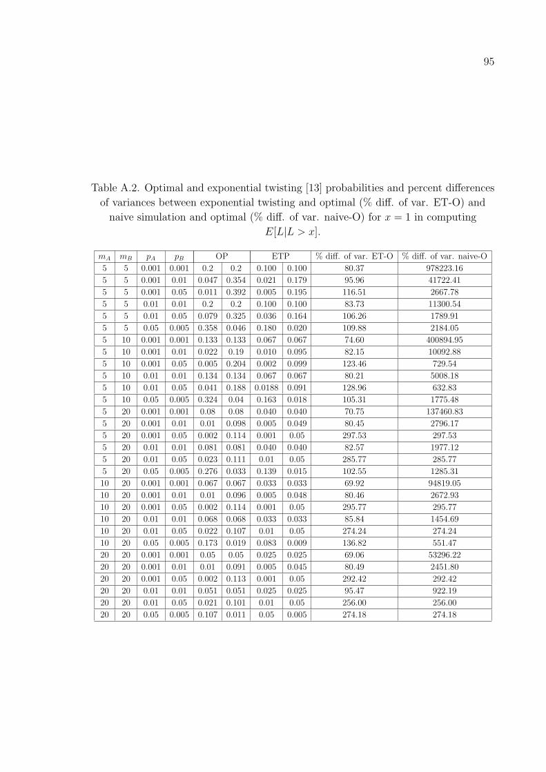
95



naive simulation and optimal (% diff. of var. naive-O) for x = 1 in computing

E[L|L > x].


5 5 0.001 0.001 0.2 0.2 0.100 0.100 80.37 978223.16

5 5 0.001 0.01 0.047 0.354 0.021 0.179 95.96 41722.41

5 5 0.001 0.05 0.011 0.392 0.005 0.195 116.51 2667.78

5 5 0.01 0.01 0.2 0.2 0.100 0.100 83.73 11300.54

5 5 0.01 0.05 0.079 0.325 0.036 0.164 106.26 1789.91

5 5 0.05 0.005 0.358 0.046 0.180 0.020 109.88 2184.05

5 10 0.001 0.001 0.133 0.133 0.067 0.067 74.60 400894.95

5 10 0.001 0.01 0.022 0.19 0.010 0.095 82.15 10092.88

5 10 0.001 0.05 0.005 0.204 0.002 0.099 123.46 729.54

5 10 0.01 0.01 0.134 0.134 0.067 0.067 80.21 5008.18

5 10 0.01 0.05 0.041 0.188 0.0188 0.091 128.96 632.83

5 10 0.05 0.005 0.324 0.04 0.163 0.018 105.31 1775.48

5 20 0.001 0.001 0.08 0.08 0.040 0.040 70.75 137460.83

5 20 0.001 0.01 0.01 0.098 0.005 0.049 80.45 2796.17

5 20 0.001 0.05 0.002 0.114 0.001 0.05 297.53 297.53

5 20 0.01 0.01 0.081 0.081 0.040 0.040 82.57 1977.12

5 20 0.01 0.05 0.023 0.111 0.01 0.05 285.77 285.77

5 20 0.05 0.005 0.276 0.033 0.139 0.015 102.55 1285.31

10 20 0.001 0.001 0.067 0.067 0.033 0.033 69.92 94819.05

10 20 0.001 0.01 0.01 0.096 0.005 0.048 80.46 2672.93

10 20 0.001 0.05 0.002 0.114 0.001 0.05 295.77 295.77

10 20 0.01 0.01 0.068 0.068 0.033 0.033 85.84 1454.69

10 20 0.01 0.05 0.022 0.107 0.01 0.05 274.24 274.24

10 20 0.05 0.005 0.173 0.019 0.083 0.009 136.82 551.47

20 20 0.001 0.001 0.05 0.05 0.025 0.025 69.06 53296.22

20 20 0.001 0.01 0.01 0.091 0.005 0.045 80.49 2451.80

20 20 0.001 0.05 0.002 0.113 0.001 0.05 292.42 292.42

20 20 0.01 0.01 0.051 0.051 0.025 0.025 95.47 922.19

20 20 0.01 0.05 0.021 0.101 0.01 0.05 256.00 256.00

20 20 0.05 0.005 0.107 0.011 0.05 0.005 274.18 274.18

96



naive simulation and optimal (% diff. of var. naive-O) for x = 5 in computing

P (L > x).


5 5 0.001 0.001 0.598 0.599 0.500 0.500 29.77 1.60E17

5 5 0.001 0.01 0.338 0.857 0.239 0.761 46.83 3.88E13

5 5 0.001 0.05 0.248 0.957 0.121 0.879 94.72 3.07E10

5 5 0.01 0.01 0.598 0.599 0.500 0.500 29.88 1.68E11

5 5 0.01 0.05 0.408 0.797 0.305 0.695 38.10 6.92E8

5 5 0.05 0.005 0.858 0.337 0.764 0.236 47.68 2.63E9

5 10 0.001 0.001 0.398 0.399 0.333 0.333 19.77 5.26E15

5 10 0.001 0.01 0.098 0.548 0.078 0.461 24.85 8.81E10

5 10 0.001 0.05 0.02 0.586 0.0180 0.491 28.42 1.14E7

5 10 0.01 0.01 0.398 0.399 0.333 0.333 19.90 5.81E9

5 10 0.01 0.05 0.168 0.52 0.129 0.436 23.37 4621209.84

5 10 0.05 0.005 0.768 0.219 0.672 0.164 30.14 5.00E8

5 20 0.001 0.001 0.238 0.24 0.200 0.200 15.54 1.30E14

5 20 0.001 0.01 0.04 0.291 0.031 0.24 16.61 5.94E8

5 20 0.001 0.05 0.01 0.299 0.006 0.248 17.96 89757.58

5 20 0.01 0.01 0.238 0.24 0.200 0.200 15.75 1.60E8

5 20 0.01 0.05 0.069 0.284 0.056 0.236 17.85 67547.46

5 20 0.05 0.005 0.648 0.139 0.563 0.109 21.52 7.38E7

10 20 0.001 0.001 0.198 0.199 0.167 0.167 14.74 3.79E13

10 20 0.001 0.01 0.04 0.283 0.030 0.235 15.91 4.89E8

10 20 0.001 0.05 0.01 0.298 0.006 0.247 17.46 86410.81

10 20 0.01 0.01 0.198 0.2 0.167 0.167 14.99 4.92E7

10 20 0.01 0.05 0.069 0.27 0.052 0.224 17.02 50179.78

10 20 0.05 0.005 0.458 0.071 0.387 0.057 19.84 1995254.55

20 20 0.001 0.001 0.148 0.149 0.125 0.125 13.83 5.72E12

20 20 0.001 0.01 0.03 0.263 0.028 0.222 14.52 3.40E8

20 20 0.001 0.05 0.01 0.295 0.006 0.244 16.36 80095.11

20 20 0.01 0.01 0.148 0.149 0.125 0.125 14.19 8278042.15

20 20 0.01 0.05 0.06 0.246 0.047 0.203 16.60 29893.18

20 20 0.05 0.005 0.268 0.033 0.223 0.027 17.36 49944.99

97

Table A.4. Optimal and Exponential Twisting ( [13]) probabilities and percent

differences of variances between exponential twisting and optimal (% diff. of var.

ET-O) and naive simulation and optimal (% diff. of var. naive-O) for x = 5 in

computing E[L|L > x].


5 5 0.001 0.001 0.6 0.6 0.500 0.500 29.79 1.60E17

5 5 0.001 0.01 0.342 0.858 0.239 0.761 46.88 3.89E13

5 5 0.001 0.05 0.244 0.957 0.121 0.879 94.85 3.08E10

5 5 0.01 0.01 0.6 0.6 0.500 0.500 29.91 1.68E11

5 5 0.01 0.05 0.404 0.796 0.305 0.695 38.20 6.96E8

5 5 0.05 0.005 0.861 0.338 0.764 0.236 47.81 2.64E9

5 10 0.001 0.001 0.4 0.4 0.333 0.333 19.78 5.26E15

5 10 0.001 0.01 0.101 0.55 0.078 0.461 24.94 8.85E10

5 10 0.001 0.05 0.024 0.588 0.018 0.491 29.22 1.17E7

5 10 0.01 0.01 0.4 0.4 0.333 0.333 19.94 5.84E9

5 10 0.01 0.05 0.164 0.519 0.129 0.436 23.60 4713387.76

5 10 0.05 0.005 0.764 0.218 0.672 0.164 30.25 5.04E8

5 20 0.001 0.001 0.24 0.24 0.200 0.200 15.56 1.30E14

5 20 0.001 0.01 0.038 0.291 0.031 0.242 16.72 6.00E8

5 20 0.001 0.05 0.008 0.299 0.006 0.248 18.73 94311.58

5 20 0.01 0.01 0.24 0.24 0.200 0.200 15.81 1.62E8

5 20 0.01 0.05 0.069 0.284 0.056 0.236 18.29 70992.21

5 20 0.05 0.005 0.645 0.139 0.563 0.109 21.61 7.46E7

10 20 0.001 0.001 0.2 0.2 0.1676 0.167 14.77 3.80E13

10 20 0.001 0.01 0.036 0.282 0.030 0.235 16.38 4.96E8

10 20 0.001 0.05 0.008 0.297 0.006 0.247 18.65 91151.17

10 20 0.01 0.01 0.2 0.2 0.167 0.167 15.08 5.00E7

10 20 0.01 0.05 0.065 0.269 0.052 0.224 17.92 53131.52

10 20 0.05 0.005 0.458 0.071 0.387 0.057 20.00 2043266.41

20 20 0.001 0.001 0.15 0.15 0.125 0.125 13.89 5.74E12

20 20 0.001 0.01 0.034 0.266 0.028 0.222 15.83 3.47E8

20 20 0.001 0.05 0.0080 0.294 0.006 0.244 18.47 85220.65

20 20 0.01 0.01 0.15 0.15 0.125 0.125 14.34 8459243.87

20 20 0.01 0.05 0.057 0.244 0.047 0.203 17.50 31860.70

20 20 0.05 0.005 0.268 0.033 0.223 0.027 17.84 52699.03

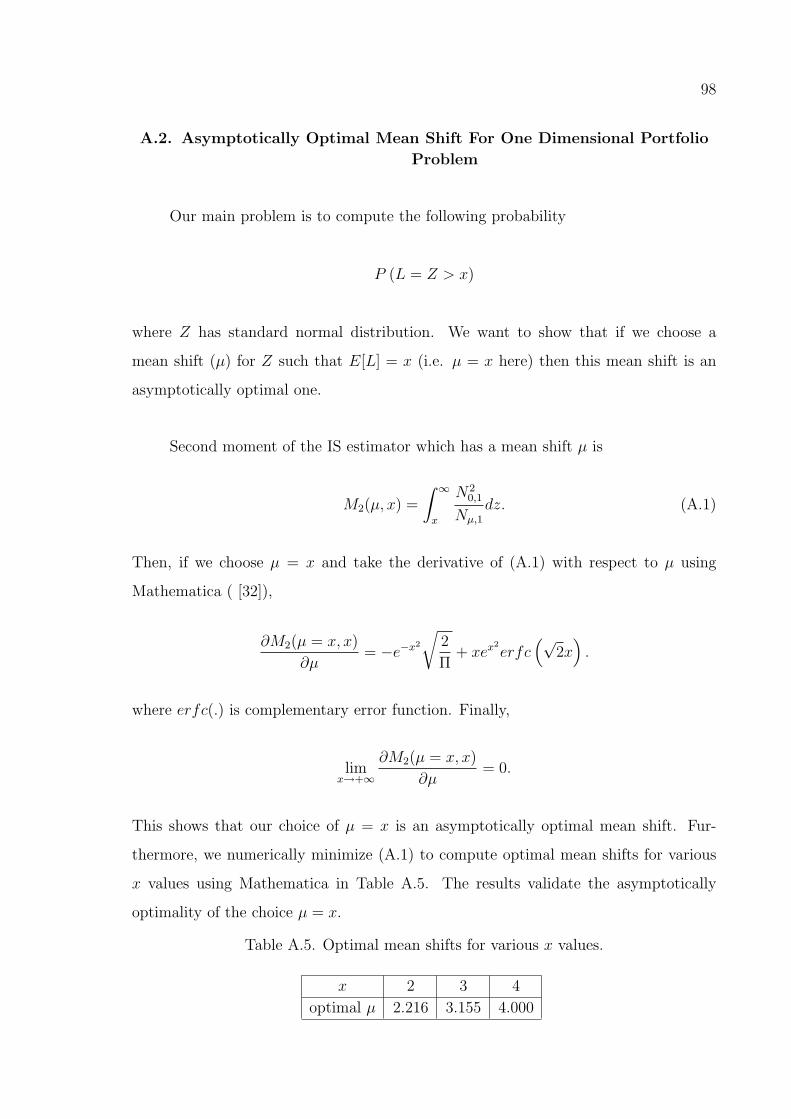
98

A.2. Asymptotically Optimal Mean Shift For One Dimensional Portfolio

Problem

Our main problem is to compute the following probability

P (L = Z > x)

where Z has standard normal distribution. We want to show that if we choose a

mean shift (µ) for Z such that E[L] = x (i.e. µ = x here) then this mean shift is an

asymptotically optimal one.

Second moment of the IS estimator which has a mean shift µ is

M2(µ, x) =

∫ ∞x

N20,1

Nµ,1

dz. (A.1)

Then, if we choose µ = x and take the derivative of (A.1) with respect to µ using

Mathematica ( [32]),

∂M2(µ = x, x)

∂µ= −e−x2

√2

Π+ xex

2

erfc(√

2x).

where erfc(.) is complementary error function. Finally,

limx→+∞

∂M2(µ = x, x)

∂µ= 0.

This shows that our choice of µ = x is an asymptotically optimal mean shift. Fur-

thermore, we numerically minimize (A.1) to compute optimal mean shifts for various

x values using Mathematica in Table A.5. The results validate the asymptotically

optimality of the choice µ = x.

Table A.5. Optimal mean shifts for various x values.

x 2 3 4

optimal µ 2.216 3.155 4.000

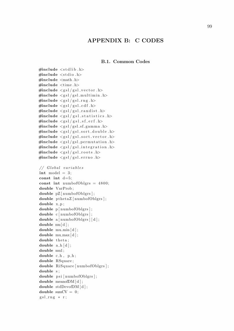
99

APPENDIX B: C CODES

B.1. Common Codes

#include <s t d l i b . h>#include <s t d i o . h>#include <math . h>#include <time . h>#include <g s l / g s l v e c t o r . h>#include <g s l / gs l mu l t imin . h>#include <g s l / g s l r n g . h>#include <g s l / g s l c d f . h>#include <g s l / g s l r a n d i s t . h>#include <g s l / g s l s t a t i s t i c s . h>#include <g s l / g s l s f e r f . h>#include <g s l / gs l s f gamma . h>#include <g s l / g s l s o r t d o ub l e . h>#include <g s l / g s l s o r t v e c t o r . h>#include <g s l / gs l pe rmutat i on . h>#include <g s l / g s l i n t e g r a t i o n . h>#include <g s l / g s l r o o t s . h>#include <g s l / g s l e r r n o . h>

// Globa l v a r i a b l e sint model = 3 ;const int d=5;const int numbofOblgrs = 4800 ;double VarProb ;double pZ [ numbofOblgrs ] ;double pthetaZ [ numbofOblgrs ] ;double x p ;double p [ numbofOblgrs ] ;double c [ numbofOblgrs ] ;double a [ numbofOblgrs ] [ d ] ;double mu[ d ] ;double mu min [ d ] ;double mu max [ d ] ;double theta ;double a h [ d ] ;double mu1 ;double c h , p h ;double RSquare ;double RiSquare [ numbofOblgrs ] ;double s ;double p s i [ numbofOblgrs ] ;double meanofDM [ d ] ;double stdDevofDM [ d ] ;double sumCV = 0 ;g s l r n g ∗ r ;

100

void GlassLiNumericExampleInit ( ){const g s l r n g t yp e ∗ Trand ;unsigned long randSeed ;Trand = g s l r n g d e f a u l t ;r = g s l r n g a l l o c (Trand ) ;

srand ( time (NULL) ) ;randSeed = rand ( ) ;g s l r n g s e t ( r , randSeed ) ;

// model 1 and 2for ( int i =0; i< numbofOblgrs ; i++){

i f ( model == 1){for ( int j = 0 ; j < d ; j++){

a [ i ] [ j ] = g s l rng un i f o rm ( r ) ∗ s q r t ( 1 . 0/ d ) ;

}p [ i ] = 0.01∗(1+ s i n (16∗M PI∗( i +1)/numbofOblgrs ) ) ;c [ i ] = pow( c e i l (5∗ (double ) ( i +1)/numbofOblgrs ) , 2 ) ;

}else i f ( model == 2){

a [ i ] [ 0 ] = 0 . 8 ;a [ i ] [ i /100+1] = 0 . 4 ;int k = i %100;a [ i ] [ k/10+11] = 0 . 4 ;p [ i ] = 0.01∗(1+ s i n (16∗M PI∗( i +1)/numbofOblgrs ) ) ;double c1 = 99 .0/999 ;double c0 = 1−c1 ;c [ i ] = c0 + c1 ∗( i +1);

}}

// model 3i f ( model == 3){

// Segment 1Afor ( int i =0; i< 800 ; i++){

a [ i ] [ 0 ] = 0 . 7 ;a [ i ] [ 1 ] = 0 . 5 ;a [ i ] [ 2 ] = 0 . 1 ;p [ i ] = 0 . 0 1 ;c [ i ] = 20 ;

}// Segment 1Bfor ( int i =800; i< 1600 ; i++){

a [ i ] [ 0 ] = 0 . 7 ;a [ i ] [ 1 ] = 0 . 5 ;a [ i ] [ 2 ] = 0 . 1 ;p [ i ] = 0 . 0 2 ;c [ i ] = 10 ;

}// Segment 2A

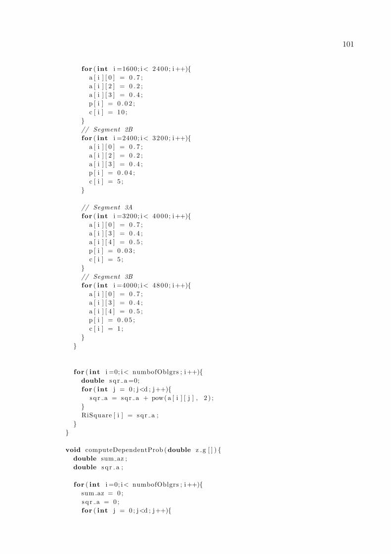
101

for ( int i =1600; i< 2400 ; i++){a [ i ] [ 0 ] = 0 . 7 ;a [ i ] [ 2 ] = 0 . 2 ;a [ i ] [ 3 ] = 0 . 4 ;p [ i ] = 0 . 0 2 ;c [ i ] = 10 ;


a [ i ] [ 0 ] = 0 . 7 ;a [ i ] [ 2 ] = 0 . 2 ;a [ i ] [ 3 ] = 0 . 4 ;p [ i ] = 0 . 0 4 ;c [ i ] = 5 ;

}

// Segment 3Afor ( int i =3200; i< 4000 ; i++){

a [ i ] [ 0 ] = 0 . 7 ;a [ i ] [ 3 ] = 0 . 4 ;a [ i ] [ 4 ] = 0 . 5 ;p [ i ] = 0 . 0 3 ;c [ i ] = 5 ;


a [ i ] [ 0 ] = 0 . 7 ;a [ i ] [ 3 ] = 0 . 4 ;a [ i ] [ 4 ] = 0 . 5 ;p [ i ] = 0 . 0 5 ;c [ i ] = 1 ;

}}

for ( int i =0; i< numbofOblgrs ; i++){double sq r a =0;for ( int j = 0 ; j<d ; j++){

sq r a = sq r a + pow( a [ i ] [ j ] , 2 ) ;}RiSquare [ i ] = sq r a ;

}}

void computeDependentProb (double z g [ ] ) {double sum az ;double sq r a ;

for ( int i =0; i< numbofOblgrs ; i++){sum az = 0 ;sq r a = 0 ;for ( int j = 0 ; j<d ; j++){

102

sum az = sum az + a [ i ] [ j ]∗ z g [ j ] ;s q r a = sq r a + pow( a [ i ] [ j ] , 2 ) ;

}pZ [ i ] = g s l c d f ugau s s i an P ( ( sum az+g s l c d f ugau s s i an P inv (p [ i ] ) ) / sq r t (1− sq r a ) ) ;

}}

void computeTwistedDependentProb (double z g [ ] ) {for ( int i =0; i< numbofOblgrs ; i++){

pthetaZ [ i ] = pZ [ i ]∗ exp ( theta ∗c [ i ] ) / (1 +pZ [ i ] ∗ ( exp ( theta ∗c [ i ] ) −1) ) ;

}}

double computeLoss ( ){double l o s s = 0 ;for ( int i =0; i<numbofOblgrs ; i++){

i f ( g s l r ng un i f o rm ( r ) < pthetaZ [ i ] ) {l o s s = l o s s + c [ i ] ;

}}return l o s s ;

}

double computeAverageProbDependent ( ){double avrg = 0 ;for ( int j =0; j<numbofOblgrs ; j++){

avrg = avrg + pZ [ j ] / numbofOblgrs ;}return avrg ;

}

// Bi s ec t i on method to s o l v e t h e t a .double solveThetaXZ (double z g [ ] ) {

int counter = 0 ;double a=0,b ;double va , vb , vc ;double de l t a = 0 . 00001 ;

double expected = 0 ;for ( int i =0; i<numbofOblgrs ; i++){

expected = expected + pZ [ i ]∗ c [ i ] ;}i f ( expected >= x p )

return 0 ;

va = theta y Equat ion ( a ) ;b = 0 . 0 1 ;while ( t rue ){

counter++;vb = theta y Equat ion (b ) ;

103

i f ( va∗vb<0){break ;

}b = 10∗b ;i f ( counter > 10){

return −1;}

}

double c ;

counter = 0 ;c = ( a+b )/2 ;vc = theta y Equat ion ( c ) ;while ( f abs ( vc)>de l t a ){

counter++;

i f ( counter > 1000){return −1;

}

i f ( va∗vc<0){b = c ;vb = theta y Equat ion (b ) ;

}else {

a = c ;va = theta y Equat ion ( a ) ;

}c = ( a+b )/2 ;vc = theta y Equat ion ( c ) ;

}return c ;

}

double solveThetaXZ Newton (double z g [ ] ) {double p0 = 0 . 1 ;double p ;double de l t a = 0 . 0 0 1 ;int count = 1 ;

while (1){p = p0 − theta y Equat ion ( p0 ) / derv theta y Equat ion ( p0 ) ;i f ( count == 3 | | f abs (p−p0 ) < de l t a )

break ;count ++;p0 = p ;

}i f ( f abs (p−p0 ) < de l t a )

return p ;else

return 0 ;

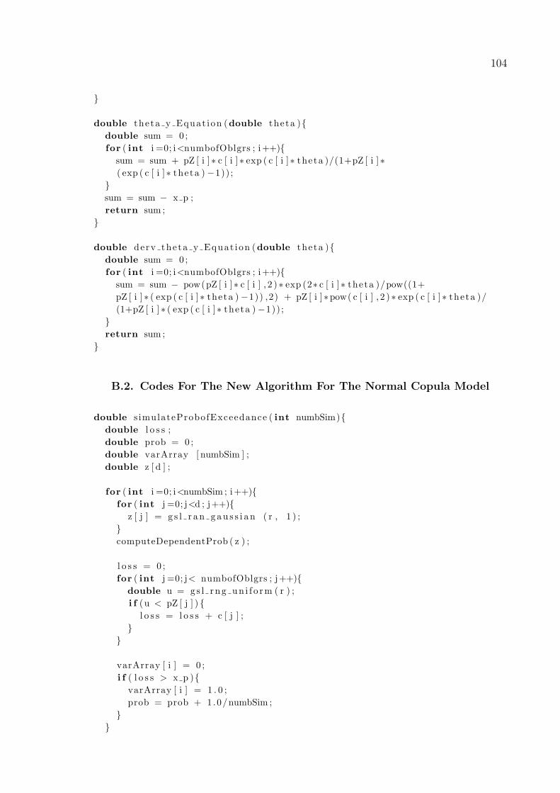
104

}

double theta y Equat ion (double theta ){double sum = 0 ;for ( int i =0; i<numbofOblgrs ; i++){

sum = sum + pZ [ i ]∗ c [ i ]∗ exp ( c [ i ]∗ theta )/(1+pZ [ i ]∗( exp ( c [ i ]∗ theta )−1)) ;

}sum = sum − x p ;return sum ;

}

double derv theta y Equat ion (double theta ){double sum = 0 ;for ( int i =0; i<numbofOblgrs ; i++){

sum = sum − pow(pZ [ i ]∗ c [ i ] , 2 ) ∗ exp (2∗ c [ i ]∗ theta )/pow((1+pZ [ i ] ∗ ( exp ( c [ i ]∗ theta )−1)) ,2) + pZ [ i ]∗pow( c [ i ] , 2 ) ∗ exp ( c [ i ]∗ theta )/(1+pZ [ i ] ∗ ( exp ( c [ i ]∗ theta )−1)) ;

}return sum ;

}

B.2. Codes For The New Algorithm For The Normal Copula Model

double s imulateProbofExceedance ( int numbSim){double l o s s ;double prob = 0 ;double varArray [ numbSim ] ;double z [ d ] ;

for ( int i =0; i<numbSim ; i++){for ( int j =0; j<d ; j++){

z [ j ] = g s l r a n g au s s i a n ( r , 1 ) ;}computeDependentProb ( z ) ;

l o s s = 0 ;for ( int j =0; j< numbofOblgrs ; j++){

double u = gs l rng un i f o rm ( r ) ;i f (u < pZ [ j ] ) {

l o s s = l o s s + c [ j ] ;}

}

varArray [ i ] = 0 ;i f ( l o s s > x p ){

varArray [ i ] = 1 . 0 ;prob = prob + 1.0/numbSim ;

}}

105

double var iance = g s l s t a t s v a r i a n c e ( varArray , 1 , numbSim ) ;double c on f i n t e r = 1 .96 ∗ pow( var iance /numbSim , 0 . 5 ) ;double lowerLim = prob − c on f i n t e r ;double upperLim = prob + con f i n t e r ;

return var iance ;}

double s imulateISProbofExceedance ( int numbSim){double l o s s ;double varArray [ numbSim ] ;double prob = 0 ;double expectedLoss = 0 ;double z [ d ] ;double l i k e l i h o odRa t i o ;

double mu muT = 0 ;for ( int k=0;k< d ; k++){

mu muT = mu muT + mu[ k ]∗mu[ k ] ;}


z [ j ] = g s l r a n g au s s i a n ( r , 1) + mu[ j ] ;}

computeDependentProb ( z ) ;

expectedLoss = 0 ;for ( int k=0;k< numbofOblgrs ; k++){

expectedLoss = expectedLoss + pZ [ k ]∗ c [ k ] ;}

i f ( expectedLoss >= x p )theta = 0 ;

else {// t h e t a = solveThetaXZ ( z ) ;

theta = solveThetaXZ Newton ( z ) ;}

computeTwistedDependentProb ( z ) ;

l o s s = computeLoss ( ) ;

double sum = 0 ;for ( int k=0;k< numbofOblgrs ; k++){

sum = sum + log (1 + pZ [ k ] ∗ ( exp ( theta ∗c [ k ] ) −1) ) ;}double mu zT = 0 ;for ( int k=0;k< d ; k++){

mu zT = mu zT + mu[ k ]∗ z [ k ] ;

106

}

varArray [ i ] = 0 ;

i f ( l o s s > x p ){l i k e l i h o odRa t i o = exp(− theta ∗ l o s s + sum)∗ exp(−mu zT+mu muT/2 ) ;varArray [ i ] = l i k e l i h o odRa t i o ;prob = prob + varArray [ i ] / numbSim ;

}}

double var iance = g s l s t a t s v a r i a n c e ( varArray , 1 , numbSim ) ;double c on f i n t e r = 1 .96 ∗ pow( var iance /numbSim , 0 . 5 ) ;

// doub le lowerLim = prob − c on f i n t e r ;// doub le upperLim = prob + con f i n t e r ;

return prob ;}

double s imulateProbofExceedanceOuterISInnerReplGeometr ic ( int numbSim){double varArray [ numbSim ] ;double prob = 0 ;double avrgDepProb ;int numInnerRepl ;double probIns ide ;double expectedAverage = 0 ;int l a s tP o s i t o n o fD e f l t ;double z [ d ] ;


z [ j ] = g s l r a n g au s s i a n ( r , 1) + mu[ j ] ;}computeDependentProb ( z ) ;

avrgDepProb = computeAverageProbDependent ( ) ;

numInnerRepl = GSL MIN( ( int ) (1/ avrgDepProb ) ,GSL MAX(100 , numbofOblgrs ) ) ;

double l o s s [ numInnerRepl ] ;

p robIns ide = 0 ;for ( int n=0;n<numInnerRepl ; n++){

l o s s [ n ] = 0 ;}

for ( int j =0; j<numbofOblgrs ; j++){l a s tP o s i t o n o fD e f l t = g s l r an g e ome t r i c ( r , pZ [ j ] ) − 1 ;

while ( l a s tP o s i t o n o fD e f l t < numInnerRepl &&l a s tPo s i t o n o fD e f l t >= 0) {

107

l o s s [ l a s tPo s i t o n o fD e f l t ] = l o s s [ l a s tP o s i t o n o fD e f l t ] + c [ j ] ;l a s tP o s i t o n o fD e f l t = l a s tPo s i t o n o fD e f l t +g s l r an g e ome t r i c ( r , pZ [ j ] ) ;

}}

for ( int n=0;n<numInnerRepl ; n++) {i f ( l o s s [ n ] > x p ) {

probIns ide = probIns ide + 1.0/ numInnerRepl ;}

}

double mu zT = 0 ;double mu muT = 0 ;for ( int k=0;k< d ; k++){

mu muT = mu muT + mu[ k ]∗mu[ k ] ;mu zT = mu zT + mu[ k ]∗ z [ k ] ;

}

varArray [ i ] = exp(−mu zT+mu muT/2) ∗ probIns ide ;expectedAverage = expectedAverage + exp(−mu zT+mu muT/2)/numbSim ;prob = prob + varArray [ i ] / numbSim ;

}

double var iance = g s l s t a t s v a r i a n c e ( varArray , 1 , numbSim ) ;double c on f i n t e r = 1 .96 ∗ pow( var iance /numbSim , 0 . 5 ) ;double lowerLim = prob − c on f i n t e r ;double upperLim = prob + con f i n t e r ;return var iance ;

}

double s imu la teNa iveExpec tedShor t f a l l ( int numbSim){double l o s s ;double varArray [ numbSim ] ;double expectedVal = 0 ;double z [ d ] ;double sumDen = 0 ;double l i k e l i h o odRa t i o ;


z [ j ] = g s l r a n g au s s i a n ( r , 1 ) ;}

computeDependentProb ( z ) ;l o s s = 0 ;

for ( int i =0; i<numbofOblgrs ; i++){i f ( g s l r ng un i f o rm ( r ) < pZ [ i ] ) {

l o s s = l o s s + c [ i ] ;

108

}}

varArray [ i ] = 0 ;

i f ( l o s s >= x p ){varArray [ i ] = l o s s ;sumDen = sumDen + 1 ;expectedVal = expectedVal + varArray [ i ] ;

}}

expectedVal = expectedVal / sumDen ;

double var iance = 0 ;for ( int i =0; i<numbSim ; i++){

i f ( varArray [ i ] > 0)var iance = var iance + pow( varArray [ i ] − expectedVal , 2 ) ;

}

var iance = numbSim ∗ var iance / pow(sumDen , 2 ) ;

double c on f i n t e r = 1 .96 ∗ pow( var iance /numbSim , 0 . 5 ) ;double lowerLim = expectedVal − c on f i n t e r ;double upperLim = expectedVal + con f i n t e r ;return expectedVal ;

}

double s imu la t e ISExpec t edSho r t f a l l ( int numbSim){double l o s s ;double varArray [ numbSim ] ;double l i k e l i h o odRa t i o [ numbSim ] ;double expectedVal = 0 ;double z [ d ] ;double suml ike l ihoodRat io = 0 ;






double expectedLoss = 0 ;for ( int k=0;k< numbofOblgrs ; k++){

109



else {theta = solveThetaXZ Newton ( z ) ;

}



varArray [ i ] = 0 ;l i k e l i h o odRa t i o [ i ] = 0 ;

i f ( l o s s >= x p ){double sum = 0 ;for ( int k=0;k< numbofOblgrs ; k++){

sum = sum + log (1 + pZ [ k ] ∗ ( exp ( theta ∗c [ k ] ) −1) ) ;}

double mu zT = 0 ;for ( int k=0;k< d ; k++){

mu zT = mu zT + mu[ k ]∗ z [ k ] ;}

l i k e l i h o odRa t i o [ i ]=exp(− theta ∗ l o s s + sum)∗ exp(−mu zT+mu muT/2 ) ;

varArray [ i ] = l o s s ;

suml ike l ihoodRat io = suml ike l ihoodRat io + l i k e l i h o odRa t i o [ i ] ;

expectedVal = expectedVal + varArray [ i ]∗ l i k e l i h o odRa t i o [ i ] ;}

}

expectedVal = expectedVal / suml ike l ihoodRat io ;


i f ( l i k e l i h o odRa t i o [ i ] > 0)var iance = var iance+pow( l i k e l i h o odRa t i o [ i ] , 2 ) ∗pow( varArray [ i ]− expectedVal , 2 ) ;

}

var iance = numbSim ∗ var iance / pow( suml ike l ihoodRat io , 2 ) ;

double c on f i n t e r = 1 .96 ∗ pow( var iance /numbSim , 0 . 5 ) ;double lowerLim = expectedVal − c on f i n t e r ;double upperLim = expectedVal + con f i n t e r ;

110

return expectedVal ;}

double s imulateExpectedShort fa l lOuter ISInnerReplGeometr i c ( int numbSim){double varArray [ numbSim ] ;double l i k e l i h o odRa t i o [ numbSim ] ;double expectedVal = 0 ;double avrgDepProb ;int numInnerRepl ;double expectedAverageIns ide ;int l a s tP o s i t o n o fD e f l t ;double z [ d ] ;double suml ike l ihoodRat io = 0 ;




z [ j ] = g s l r a n g au s s i a n ( r , 1) + mu[ j ] ;}computeDependentProb ( z ) ;




for ( int n=0;n<numInnerRepl ; n++){l o s s [ n ] = 0 ;

}




}}

expectedAverageIns ide = 0 ;for ( int n=0;n<numInnerRepl ; n++) {

expectedAverageIns ide = expectedAverageIns ide +l o s s [ n ] / numInnerRepl ;

}

111

varArray [ i ] = 0 ;l i k e l i h o odRa t i o [ i ] = 0 ;

i f ( expectedAverageIns ide >= x p ){double mu zT = 0 ;for ( int k=0;k< d ; k++){

mu zT = mu zT + mu[ k ]∗ z [ k ] ;}

l i k e l i h o odRa t i o [ i ] = exp(−mu zT + mu muT/2 ) ;

varArray [ i ] = expectedAverageIns ide ;

suml ike l ihoodRat io = suml ike l ihoodRat io + l i k e l i h o odRa t i o [ i ] ;

expectedVal = expectedVal + varArray [ i ]∗ l i k e l i h o odRa t i o [ i ] ;}

}

expectedVal = expectedVal / suml ike l ihoodRat io ;


i f ( l i k e l i h o odRa t i o [ i ] > 0)var iance = var iance + pow( l i k e l i h o odRa t i o [ i ] , 2 ) ∗pow( varArray [ i ] − expectedVal , 2 ) ;

}

var iance = numbSim ∗ var iance / pow( suml ike l ihoodRat io , 2 ) ;

double c on f i n t e r = 1 .96 ∗ pow( var iance /numbSim , 0 . 5 ) ;double lowerLim = expectedVal − c on f i n t e r ;double upperLim = expectedVal + con f i n t e r ;

return var iance ;}

double expectedLossGrtrThnVaRNormalDist (double mean ,double sigma , double x ){

double xs = (x−mean)/ sigma ;double expectedVal ;i f ( g s l s f e r f c ( xs / sq r t ( 2 ) ) > pow(10 ,−40))

expectedVal = exp(−pow( xs , 2 ) / 2 ) ∗ s q r t (2/M PI) /g s l s f e r f c ( xs / sq r t ( 2 ) ) ;

elseexpectedVal = 0 ;

expectedVal = sigma∗ expectedVal + mean ;return expectedVal ;

}

112

void simulateISProbofExceedanceVaR ( int numbSim , double x IS , int N){double varArray [N ] [ numbSim ] ;double prob [N ] ;double z [ d ] ;double u ;int key ;double x [N ] ;double probIns ide [N ] ;double expectedLoss , l o s s , l i k e l i h o odRa t i o ;

// A l l IS d i s t r i b u t i o n w i l l be f o r x . .x p = x IS ;

for ( int l = 0 ; l < N; l++){x [ l ] = l ∗500 + 500 ;prob [ l ] = 0 ;

}














sum = sum + log (1 + pZ [ k ] ∗ ( exp ( theta ∗c [ k ] ) −1) ) ;}double mu zT = 0 ;

113

for ( int k=0;k< d ; k++){mu zT = mu zT + mu[ k ]∗ z [ k ] ;

}

l i k e l i h o odRa t i o = exp(− theta ∗ l o s s + sum)∗ exp(−mu zT + mu muT/2 ) ;

for ( int l =0; l<N; l++){varArray [ l ] [ i ] = 0 ;i f ( l o s s > x [ l ] ) {

varArray [ l ] [ i ] = l i k e l i h o odRa t i o ;prob [ l ] = prob [ l ] + varArray [ l ] [ i ] / numbSim ;

}}

}

for ( int l = 0 ; l < N; l++){

double var iance = g s l s t a t s v a r i a n c e ( varArray [ l ] , 1 , numbSim ) ;double c on f i n t e r = 1 .96 ∗ pow( var iance /numbSim , 0 . 5 ) ;

p r i n t f ( ”x [ l ] %l f \n” , x [ l ] ) ;p r i n t f ( ”prob IS %.8 l f \n” , prob [ l ] ) ;p r i n t f ( ” c on f i n t e r IS %.12 l f \n” , c o n f i n t e r ) ;p r i n t f ( ”\n” ) ;

double lowerLim = prob [ l ] − c on f i n t e r ;double upperLim = prob [ l ] + c on f i n t e r ;

}

}

void simulateNaiveProbofExceedanceVaR ( int numbSim , int N){double varArray [N ] [ numbSim ] ;double prob [N ] ;double z [ d ] ;double x [N ] ;double probIns ide [N ] ;double l o s s ;


}


z [ j ] = g s l r a n g au s s i a n ( r , 1 ) ;}computeDependentProb ( z ) ;

l o s s = 0 ;for ( int j =0; j< numbofOblgrs ; j++){

114

double u = gs l rng un i f o rm ( r ) ;i f (u < pZ [ j ] ) {

l o s s = l o s s + c [ j ] ;}

}

for ( int l = 0 ; l < N; l++){varArray [ l ] [ i ] = 0 ;i f ( l o s s > x [ l ] ) {

varArray [ l ] [ i ] = 1 . 0 ;prob [ l ] = prob [ l ] + varArray [ l ] [ i ] / numbSim ;

}}

}

for ( int l = 0 ; l < N; l++){

double var iance = g s l s t a t s v a r i a n c e ( varArray [ l ] , 1 , numbSim ) ;

p r i n t f ( ”x [ l ] %l f \n” , x [ l ] ) ;p r i n t f ( ”prob naive %.8 l f \n” , prob [ l ] ) ;p r i n t f ( ” var i ance naive %.12 l f \n” , var i ance ) ;p r i n t f ( ”\n” ) ;

// doub le c on f i n t e r = 1.96 ∗ pow( var iance /numbSim , 0 . 5 ) ;// doub le lowerLim = prob [ l ] − c on f i n t e r ;// doub le upperLim = prob [ l ] + con f i n t e r ;}

}

void s imulateProbofExceedanceOuterISInnerReplGeometricDensityMixtureVaRNormalEq( int numbSim , double xmin , double xmax , int N){

double varArray [N ] [ numbSim ] ;double prob [N ] ;double avrgDepProb ;int numInnerRepl ;double expectedAverage = 0 ;int l a s tP o s i t o n o fD e f l t ;double z [ d ] ;double u ;int key ;double x [N ] ;double probIns ide [N ] ;


}

for ( int i =0; i<numbSim ; i++){

115

for ( int j =0; j<d ; j++){z [ j ] = g s l r a n g au s s i a n ( r , stdDevofDM [ j ] ) + meanofDM [ j ] ;

}





for ( int l =0; l<N; l++){probIns ide [ l ] = 0 ;

}


}




}}

for ( int n=0;n<numInnerRepl ; n++) {

for ( int l =0; l<N; l++){i f ( l o s s [ n ] > x [ l ] ) {

probIns ide [ l ] = probIns ide [ l ] + 1 .0/ numInnerRepl ;}

}}

double outerWeight = 1 . 0 ;for ( int k=0;k< d ; k++){

outerWeight = outerWeight ∗ 2 / ( exp (mu min [ k ]∗ z [ k ] −0 .5∗mu min [ k ]∗mu min [ k ] ) +exp (mu max [ k ]∗ z [ k ] − 0 .5∗mu max [ k ]∗mu max [ k ] ) ) ;

}

116

for ( int l =0; l<N; l++){varArray [ l ] [ i ] = outerWeight ∗ probIns ide [ l ] ;prob [ l ] = prob [ l ] + varArray [ l ] [ i ] / numbSim ;

}}

for ( int k = 0 ; k < N; k++){

double var iance = g s l s t a t s v a r i a n c e ( varArray [ k ] , 1 , numbSim ) ;p r i n t f ( ”x [ l ] %l f \n” , x [ k ] ) ;p r i n t f ( ”prob new %.8 l f \n” , prob [ k ] ) ;p r i n t f ( ” var i ance new %.12 l f \n” , var i ance ) ;p r i n t f ( ”\n” ) ;

double c on f i n t e r = 1 .96 ∗ pow( var iance /numbSim , 0 . 5 ) ;double lowerLim = prob [ k ] − c on f i n t e r ;double upperLim = prob [ k ] + c on f i n t e r ;

}

}

void densityMixtureNormalApprox (double xmin , double xmax){x p = xmin ;solveOptMeanShiftNormalApprox ( ) ;for ( int k=0;k< d ; k++){

mu min [ k ] = mu[ k ] ;}

x p = xmax ;solveOptMeanShiftNormalApprox ( ) ;for ( int k=0;k< d ; k++){

mu max [ k ] = mu[ k ] ;}

}

void normalEquivalentofDMNormalApprox (double xmin , double xmax){densityMixtureNormalApprox (xmin , xmax ) ;

for ( int k=0;k< d ; k++){meanofDM [ k ] = 0 .5∗mu min [ k ] + 0 .5∗mu max [ k ] ;stdDevofDM [ k ] = pow(1 + 0 .25∗ (pow(mu min [ k ] , 2 ) +pow(mu max [ k ] , 2 ) ) − 0 .5∗mu min [ k ]∗mu max [ k ] , 0 . 5 ) ;

}

}

void simulateISESWide x ( int numbSim , double x IS , int N){double varArray [ numbSim ] ;double l i k e l i h o odRa t i o [ numbSim ] ;int i sOver x [N ] [ numbSim ] ;double suml ike l ihoodRat io [N] , expectedVal [N ] ;

117

double z [ d ] ;double x [N ] ;double expectedLoss , l o s s ;

// A l l IS d i s t r i b u t i o n w i l l be f o r x . .x p = x IS ;

for ( int l = 0 ; l < N; l++){x [ l ] = l ∗50 + 500 ;suml ike l ihoodRat io [ l ] = 0 ;expectedVal [ l ] = 0 ;

}















mu zT = mu zT + mu[ k ]∗ z [ k ] ;}varArray [ i ] = l o s s ;l i k e l i h o odRa t i o [ i ] = exp(− theta ∗ l o s s + sum)∗ exp(−mu zT + mu muT/2 ) ;

118

for ( int l =0; l<N; l++){i sOver x [ l ] [ i ] = 0 ;i f ( l o s s >= x [ l ] ) {

i sOver x [ l ] [ i ] = 1 ;

suml ike l ihoodRat io [ l ] = suml ike l ihoodRat io [ l ] +l i k e l i h o odRa t i o [ i ] ;

expectedVal [ l ] = expectedVal [ l ] + l o s s ∗ l i k e l i h o odRa t i o [ i ] ;}

}}

for ( int l = 0 ; l < N; l++){expectedVal [ l ] = expectedVal [ l ] / suml ike l ihoodRat io [ l ] ;


i f ( i sOver x [ l ] [ i ] > 0)var iance = var iance + pow( l i k e l i h o odRa t i o [ i ] , 2 ) ∗pow( varArray [ i ] − expectedVal [ l ] , 2 ) ;

}

var iance = numbSim ∗ var iance / pow( suml ike l ihoodRat io [ l ] , 2 ) ;double c on f i n t e r = 1 .96 ∗ pow( var iance /numbSim , 0 . 5 ) ;

p r i n t f ( ”x [ l ] %l f \n” , x [ l ] ) ;p r i n t f ( ”ES IS %.8 l f \n” , expectedVal [ l ] ) ;p r i n t f ( ” c on f i n t e r IS %.12 l f \n” , c o n f i n t e r ) ;p r i n t f ( ”\n” ) ;

double lowerLim = expectedVal [ l ] − c on f i n t e r ;double upperLim = expectedVal [ l ] + c on f i n t e r ;

}}

void simulateESOuterISInnerReplGeometricWide x ( int numbSim , int N){double varArray [ numbSim ] ;double l i k e l i h o odRa t i o [ numbSim ] ;int i sOver x [N ] [ numbSim ] ;double suml ike l ihoodRat io [N] , expectedVal [N ] ;double z [ d ] ;double x [N ] ;double expectedLoss , l o s s ;int numInnerRepl ;double expectedAverageIns ide , avrgDepProb ;int l a s tP o s i t o n o fD e f l t ;

for ( int l = 0 ; l < N; l++){x [ l ] = l ∗50 + 500 ;

119

suml ike l ihoodRat io [ l ] = 0 ;expectedVal [ l ] = 0 ;

}


z [ j ] = g s l r a n g au s s i a n ( r , stdDevofDM [ j ] ) + meanofDM [ j ] ;}






}




}}

expectedAverageIns ide = 0 ;for ( int n=0;n<numInnerRepl ; n++) {

expectedAverageIns ide = expectedAverageIns ide +l o s s [ n ] / numInnerRepl ;

}

double outerWeight = 1 . 0 ;for ( int k=0;k< d ; k++){

outerWeight = outerWeight ∗ 2 / ( exp (mu min [ k ]∗ z [ k ] −0 .5∗mu min [ k ]∗mu min [ k ] ) + exp (mu max [ k ]∗ z [ k ] −0 .5∗mu max [ k ]∗mu max [ k ] ) ) ;

}

l i k e l i h o odRa t i o [ i ] = outerWeight ;varArray [ i ] = expectedAverageIns ide ;

for ( int l =0; l<N; l++){i sOver x [ l ] [ i ] = 0 ;

120

i f ( expectedAverageIns ide >= x [ l ] ) {i sOver x [ l ] [ i ] = 1 ;

suml ike l ihoodRat io [ l ] = suml ike l ihoodRat io [ l ] +l i k e l i h o odRa t i o [ i ] ;

expectedVal [ l ] = expectedVal [ l ] +expectedAverageIns ide ∗ l i k e l i h o odRa t i o [ i ] ;

}

}}

for ( int l = 0 ; l < N; l++){expectedVal [ l ] = expectedVal [ l ] / suml ike l ihoodRat io [ l ] ;


i f ( i sOver x [ l ] [ i ] > 0)var iance = var iance + pow( l i k e l i h o odRa t i o [ i ] , 2 ) ∗pow( varArray [ i ] − expectedVal [ l ] , 2 ) ;

}

var iance = numbSim ∗ var iance / pow( suml ike l ihoodRat io [ l ] , 2 ) ;double c on f i n t e r = 1 .96 ∗ pow( var iance /numbSim , 0 . 5 ) ;

p r i n t f ( ”x [ l ] %l f \n” , x [ l ] ) ;p r i n t f ( ”ES new %.8 l f \n” , expectedVal [ l ] ) ;p r i n t f ( ” c on f i n t e r new %.12 l f \n” , c o n f i n t e r ) ;p r i n t f ( ”\n” ) ;

double lowerLim = expectedVal [ l ] − c on f i n t e r ;double upperLim = expectedVal [ l ] + c on f i n t e r ;

}}

B.3. Codes For The Comparison of Mean Shifts For IS

int solveOptMeanShiftNormalApprox ( ){

s i z e t np = d ;double par [ d ] = {1 . 0} ;

const g s l mu l t im in fm in im i z e r type ∗T =gs l mul t imin fmin imizer nms implex ;

g s l mu l t im in fm in im i z e r ∗ s = NULL;g s l v e c t o r ∗ ss , ∗x ;g s l mu l t im in func t i on minex func ;

121

s i z e t i t e r = 0 , i ;int s t a tu s ;double s i z e ;

/∗ I n i t i a l v e r t e x s i z e v e c t o r ∗/s s = g s l v e c t o r a l l o c (np ) ;

/∗ Set a l l s t ep s i z e s to 1 ∗/g s l v e c t o r s e t a l l ( ss , 1 . 0 ) ;

/∗ S t a r t i n g po in t ∗/x = g s l v e c t o r a l l o c (np ) ;

g s l v e c t o r s e t a l l (x , 2 ) ;// g s l v e c t o r s e t ( x , 0 , 2 . 2 ) ;

/∗ I n i t i a l i z e method and i t e r a t e ∗/minex func . f = &my f ;minex func . n = np ;minex func . params = (void ∗)&par ;

s = g s l mu l t im i n fm i n im i z e r a l l o c (T, np ) ;g s l mu l t im in fm in im i z e r s e t ( s , &minex func , x , s s ) ;

do{

i t e r ++;s t a tu s = g s l mu l t im i n fm i n im i z e r i t e r a t e ( s ) ;

i f ( s t a tu s )break ;

s i z e = g s l mu l t im i n fm in im i z e r s i z e ( s ) ;s t a tu s = g s l mu l t im i n t e s t s i z e ( s i z e , 1e−2);

i f ( s t a tu s == GSL SUCCESS){

// p r i n t f (” converged to minimum at \n” ) ;}

}while ( s t a tu s == GSL CONTINUE && i t e r < 10000) ;

for ( i = 0 ; i < np ; i++){mu[ i ] = g s l v e c t o r g e t ( s−>x , i ) ;}

g s l v e c t o r f r e e ( x ) ;g s l v e c t o r f r e e ( s s ) ;g s l mu l t im i n fm in im i z e r f r e e ( s ) ;

122

return s t a tu s ;}

double objec t iveFunct ionZ ( const g s l v e c t o r ∗v , void ∗params ) {double z g [ d ] ;double sum = 0 ;

for ( int j =0; j< d ; j++){z g [ j ] = g s l v e c t o r g e t (v , j ) ;

}

computeDependentProb ( z g ) ;// doub le t h e t a = solveThetaXZ Newton ( z g ) ;

double theta = solveThetaXZ ( z g ) ;

double sumsqrz = 0 ;

for ( int i =0; i< numbofOblgrs ; i++){sum = sum + log (1 + pZ [ i ] ∗ ( exp ( theta ∗c [ i ] ) −1) ) ;

}

for ( int i =0; i< d ; i++){sumsqrz = sumsqrz + pow( z g [ i ] , 2 ) ;

}

return theta ∗x p − sum + 0.5∗ sumsqrz ;}

int so lveOptMeanShi ftGlassLi ( ){

s i z e t np = d ;double par [ d ] = {1 . 0} ;

const g s l mu l t im in fm in im i z e r type ∗T =gs l mul t imin fmin imizer nms implex ;

g s l mu l t im in fm in im i z e r ∗ s = NULL;g s l v e c t o r ∗ ss , ∗x ;g s l mu l t im in func t i on minex func ;



/∗ Set a l l s t ep s i z e s to 1 ∗/g s l v e c t o r s e t a l l ( ss , 1 . 0 ) ;

/∗ S t a r t i n g po in t ∗/

123

x = g s l v e c t o r a l l o c (np ) ;

g s l v e c t o r s e t a l l (x , 2 ) ;

/∗ I n i t i a l i z e method and i t e r a t e ∗/minex func . f = &objec t iveFunct ionZ ;minex func . n = np ;minex func . params = (void ∗)&par ;


do{



s i z e = g s l mu l t im i n fm in im i z e r s i z e ( s ) ;s t a tu s = g s l mu l t im i n t e s t s i z e ( s i z e , 1e−2);

}while ( s t a tu s == GSL CONTINUE && i t e r < 10000) ;

for ( i = 0 ; i < np ; i++){

mu[ i ] = g s l v e c t o r g e t ( s−>x , i ) ;}



double my f ( const g s l v e c t o r ∗v , void ∗params ) {double ∗dp = (double ∗) params ;double z g [ d ] ;double A = 0 , B = 0 ;double f z = 1 ;

for ( int j =0; j< d ; j++){z g [ j ] = g s l v e c t o r g e t (v , j ) ;

// p r i n t f (”% l f ,\n” , z g [ j ] ) ;

}

computeDependentProb ( z g ) ;

124

for ( int i =0; i< numbofOblgrs ; i++){A = A + c [ i ]∗pZ [ i ] ;B = B + pow( c [ i ] , 2) ∗ (pZ [ i ] − pow(pZ [ i ] , 2 ) ) ;

}

// p r i n t f (”A %l f B %l f \n” , A, B) ;

for ( int j =0; j< d ; j++){f z = f z ∗ g s l r a n g au s s i a n pd f ( z g [ j ] , 1 ) ;

}

return −(1−g s l c d f ugau s s i an P ( ( x p − A) / pow(B, 0 . 5 ) ) ) ∗ f z ;}

double returnCovar iance ( int i , int j ){i f ( i == j ){

return 1 ;}else {

return 0 ;}

}

double returnCovarianceOrg ( int i , int j ){double sum = 0 ;i f ( i == j ){

return 1 ;}else {

sum = 0 ;for ( int k=0;k< d ; k++){

sum = sum + a [ i ] [ k ]∗ a [ j ] [ k ] ;}return sum ;

}}

double returnCovarianceHom ( int i , int j ){double sum = 0 ;i f ( i == j ){

return 1 ;}else {

sum = 0 ;for ( int k=0;k< d ; k++){

sum = sum + pow( a h [ k ] , 2 ) ;}return sum ;

}}

125

void computePsi ( ){for ( int k=0;k< d ; k++){

p s i [ k ] = 0 ;for ( int i =0; i< numbofOblgrs ; i++){

p s i [ k ] = ps i [ k ] + p [ i ]∗ c [ i ]∗ a [ i ] [ k ] ;}

}}

void computeRSquare ( ){computePsi ( ) ;double sum1 = 0 ;for ( int i =0; i< d ; i++){

for ( int j =0; j< d ; j++){sum1 = sum1 + ps i [ i ]∗ p s i [ j ]∗ returnCovar iance ( i , j ) ;

}}

double sum2 = 0 ;for ( int i =0; i< numbofOblgrs ; i++){

sum2 = sum2 + pow(p [ i ]∗ c [ i ] , 2) ∗ RiSquare [ i ] ;}


sum3 = sum3 + pow(p [ i ]∗ c [ i ] , 2 ) ;}


sum4 = sum4 + p [ i ]∗ c [ i ] ;}sum4 = pow(sum4 , 2 ) ;

RSquare = (sum1 − sum2) / ( sum4 − sum3 ) ;p r i n t f ( ”RSquare %l f \n” , RSquare ) ;

}

void computeS ( ){computeRSquare ( ) ;double sum = 0 ;for ( int i =0; i< d ; i++){

for ( int j =0; j< d ; j++){sum = sum + ps i [ i ]∗ p s i [ j ]∗ returnCovar iance ( i , j ) ;

}}sum = sum / RSquare ;s = pow(sum , 0 . 5 ) ;p r i n t f ( ” s %l f \n” , s ) ;

}

126

void computeHomFactorLoadings ( ){computeS ( ) ;for ( int k=0;k< d ; k++){

a h [ k ] = 0 ;for ( int i =0; i< numbofOblgrs ; i++){

a h [ k ] = a h [ k ] + p [ i ]∗ c [ i ]∗ a [ i ] [ k ] ;}a h [ k ] = a h [ k ] / s ;

}}

void homogenousPortEquivalent ( ){double sum c ;c h = 0 ;for ( int i =0; i< numbofOblgrs ; i++){

c h = c h + c [ i ] / numbofOblgrs ;sum c = sum c + c [ i ] ;

}

p h = 0 ;for ( int i =0; i< numbofOblgrs ; i++){

p h = p h + p [ i ]∗ c [ i ] / sum c ;}

computeHomFactorLoadings ( ) ;

}

double f unc t i onToInteg ra te (double x , void ∗ params ){return pow( c h ∗ g s l c d f ugau s s i an P ( ( g s l c d f ugau s s i an P inv ( p h ) +pow(RSquare , 0 . 5 )∗ x )/ sq r t (1−RSquare ) )∗ g s l r a n g au s s i a n pd f (x , 1 ) , 2 ) /g s l r a n g au s s i a n pd f (x−mu1 , 1 ) ;

}

double i n t eg ra t eExpec tedShor t f a l l f o rHomPort f ( const g s l v e c t o r ∗v ,void ∗params ) {

double ∗dp = (double ∗) params ;mu1 = g s l v e c t o r g e t (v , 0 ) ;

g s l i n t e g r a t i on wo rk spa c e ∗ w =g s l i n t e g r a t i o n wo r k s p a c e a l l o c ( 1000 ) ;double r e su l t , e r r o r ;double alpha = 1 . 0 ;

g s l f u n c t i o n F ;F . func t i on = &funct i onToInteg ra t e ;F . params = &alpha ;g s l i n t e g r a t i o n q a g s (&F, g s l c d f ugau s s i an P inv (VarProb ) ,5 , 0 , 1e−4, 1000 , w, &r e su l t , &e r r o r ) ;g s l i n t e g r a t i o n wo r k s p a c e f r e e (w) ;return r e s u l t ;

}

127

double simVarianceHomPort ( const g s l v e c t o r ∗v , void ∗params ) {double ∗dp = (double ∗) params ;double l o s s ;double z h , l i k e l i h oodRat i o , mu zT ;

//one dimensiona l mean s h i f tmu1 = g s l v e c t o r g e t (v , 0 ) ;int numbSim = 1000000;double varArray [ numbSim ] ;double prob = 0 ;

double mu muT = mu1∗mu1 ;

for ( int i =0; i<numbSim ; i++){z h = g s l r a n g au s s i a n ( r , 1) + mu1 ;l o s s = c h ∗ g s l c d f ugau s s i an P ( ( g s l c d f ugau s s i an P inv ( p h ) +pow(RSquare , 0 . 5 )∗ z h )/ sq r t (1−RSquare ) ) ;

varArray [ i ] = 0 ;i f ( z h > g s l c d f ugau s s i an P inv (VarProb ) ){

mu zT = mu1∗ z h ;l i k e l i h o odRa t i o = exp(−mu zT+mu muT/2)∗ l o s s ;varArray [ i ] = l i k e l i h o odRa t i o ;prob = prob + varArray [ i ] / numbSim ;

}}double var iance = g s l s t a t s v a r i a n c e ( varArray , 1 , numbSim ) ;return var iance ;

}

int so lveforOneDimShi ftHomogenousPort fo l io ( ){

s i z e t np = 1 ;double par [ 1 ] = {1 . 0} ;

const g s l mu l t im in fm in im i z e r type ∗T =gs l mul t imin fmin imizer nms implex ;g s l mu l t im in fm in im i z e r ∗ s = NULL;g s l v e c t o r ∗ ss , ∗x ;g s l mu l t im in func t i on minex func ;



/∗ Set a l l s t ep s i z e s to 1 ∗/g s l v e c t o r s e t a l l ( ss , 0 . 0 1 ) ;

/∗ S t a r t i n g po in t ∗/

128

x = g s l v e c t o r a l l o c (np ) ;

g s l v e c t o r s e t a l l (x , 1 ) ;// g s l v e c t o r s e t ( x , 0 , 2 . 2 ) ;

/∗ I n i t i a l i z e method and i t e r a t e ∗/// minex func . f = &simVarianceHomPort ;

minex func . f = integ ra t eExpec tedShor t f a l l f o rHomPort f ;minex func . n = np ;minex func . params = (void ∗)&par ;


do{



s i z e = g s l mu l t im i n fm in im i z e r s i z e ( s ) ;s t a tu s = g s l mu l t im i n t e s t s i z e ( s i z e , 1e−5);}while ( s t a tu s == GSL CONTINUE && i t e r < 10000) ;



void computeMultiDimShiftKalkbrenerHomPort ( ){homogenousPortEquivalent ( ) ;so lveforOneDimShi ftHomogenousPort fo l io ( ) ;for ( int i =0; i< d ; i++){

mu[ i ] = mu1 ∗ a h [ i ] / pow(RSquare , 0 . 5 ) ;p r i n t f ( ”%l f \n” , mu[ i ] ) ;

}

}

B.4. Codes For The Better Confidence Intervals For IS

double t h i r d r o o t (double x ){return GSL SIGN (x )∗pow( f a b s f ( x ) , 1 . 0 / 3 ) ;

}

double inverseTrans form (double x , double a , double b ,

129

double skewness , int numbSim){double r e s ;r e s = pow(numbSim , 0 . 5 ) ∗ 1 . 0 / ( a∗ skewness )∗ ( t h i r d r o o t (1+3∗a∗ skewness ∗(pow(numbSim,−0.5)∗x−1.0/numbSim∗b∗ skewness ))−1) ;return r e s ;

}

g s l v e c t o r ∗ upperEndLowerEndConfInt ( int n , g s l v e c t o r ∗ sample ,double exact , double beta ){

g s l v e c t o r ∗ r e s = g s l v e c t o r a l l o c ( 2 ) ;g s l v e c t o r s e t z e r o ( r e s ) ;double sigma = pow( g s l s t a t s v a r i a n c e ( sample−>data , 1 , n ) , 0 . 5 ) ;double skewness = g s l s t a t s s k ew ( sample−>data , 1 , n ) ;double temp = inverseTrans form ( g s l c d f g au s s i a n P i nv (1−beta , 1 ) ,1 . 0 /3 , 1 . 0 /6 , skewness , n ) ;double bound = gs l s t a t s mean ( sample−>data , 1 , n)−pow(n ,−0.5)∗ sigma∗temp ;

i f ( exact<bound ){g s l v e c t o r s e t ( res , 0 , 1 ) ;

}temp = inverseTrans form ( g s l c d f g au s s i a n P i nv ( beta , 1 ) ,1 . 0 /3 , 1 . 0 /6 , skewness , n ) ;bound = gs l s t a t s mean ( sample−>data , 1 , n)−pow(n ,−0.5)∗ sigma∗temp ;

i f ( exact>bound ){g s l v e c t o r s e t ( res , 1 , 1 ) ;

}return r e s ;

}

g s l v e c t o r ∗ simulatemanyLossProb ( int m, int n , double exact ,double beta ){

g s l v e c t o r ∗ res , ∗resUp , ∗ resLower , ∗ sample , ∗ f i nResu l t , ∗ r e s t S t a t ;resUp = g s l v e c t o r a l l o c (m) ;resLower = g s l v e c t o r a l l o c (m) ;r e s t S t a t = g s l v e c t o r a l l o c (m) ;

f i nRe su l t = g s l v e c t o r a l l o c ( 4 ) ;

for ( int i =0; i<m; i++){//common sample f o r both methods .sample = s imulateISProbofExceedance forCI (n ) ;// t s t a tg s l v e c t o r s e t ( r e s tS ta t , i , ( g s l s t a t s mean ( sample−>data , 1 , n)−exact )/ ( g s l s t a t s s d ( sample−>data , 1 , n)/ sq r t (n ) ) ) ;// Ha l lr e s = upperEndLowerEndConfInt (n , sample , exact , beta ) ;g s l v e c t o r s e t ( resUp , i , g s l v e c t o r g e t ( res , 0 ) ) ;g s l v e c t o r s e t ( resLower , i , g s l v e c t o r g e t ( res , 1 ) ) ;g s l v e c t o r f r e e ( sample ) ;g s l v e c t o r f r e e ( r e s ) ;

130

}// t s t a tdouble resL = 0 ;double resU = 0 ;for ( int l =0; l<m; l++){

i f ( g s l v e c t o r g e t ( r e s tS ta t , l ) < g s l c d f g au s s i a n P i nv ( 0 . 9 5 , 1 ) )resL = resL + 1 .0 / m;

i f ( g s l v e c t o r g e t ( r e s tS ta t , l ) > g s l c d f g au s s i a n P i nv ( 0 . 0 5 , 1 ) )resU = resU + 1 .0 / m;

}g s l v e c t o r s e t ( f i nResu l t , 0 , resU ) ;g s l v e c t o r s e t ( f i nResu l t , 1 , g s l s t a t s mean ( resUp−>data , 1 ,m) ) ;g s l v e c t o r s e t ( f i nResu l t , 2 , resL ) ;g s l v e c t o r s e t ( f i nResu l t , 3 , g s l s t a t s mean ( resLower−>data , 1 ,m) ) ;

g s l v e c t o r f r e e ( resLower ) ;g s l v e c t o r f r e e ( resUp ) ;g s l v e c t o r f r e e ( r e s t S t a t ) ;return f i nRe su l t ;

}

g s l v e c t o r ∗ s imulateISProbofExceedance forCI ( int numbSim){g s l v e c t o r ∗ r e s ;r e s = g s l v e c t o r a l l o c (numbSim ) ;double l o s s ;double expectedLoss = 0 ;double z [ d ] ;double l i k e l i h o odRa t i o ;










theta = solveThetaXZ Newton ( z ) ;

131

}





mu zT = mu zT + mu[ k ]∗ z [ k ] ;}

g s l v e c t o r s e t ( res , i , 0 ) ;i f ( l o s s > x p ){

l i k e l i h o odRa t i o = exp(− theta ∗ l o s s + sum) ∗exp(−mu zT+mu muT/2 ) ;

g s l v e c t o r s e t ( res , i , l i k e l i h o odRa t i o ) ;}

}

double beta = 1−0.05;

double prob = gs l s t a t s mean ( res−>data , 1 , numbSim ) ;double var iance = g s l s t a t s v a r i a n c e ( res−>data , 1 , numbSim ) ;double c on f i n t e r = g s l c d f g au s s i a n P i nv ( beta , 1 ) ∗pow( var iance /numbSim , 0 . 5 ) ;double lowerLim = prob − c on f i n t e r ;double upperLim = prob + con f i n t e r ;

p r i n t f ( ”prob GL %.8 l f \n” , prob ) ;p r i n t f ( ”upper bound t %.8 l f \n” , upperLim ) ;p r i n t f ( ” lower bound t %.8 l f \n” , lowerLim ) ;

// Ha l l CIdouble sigma = pow( g s l s t a t s v a r i a n c e ( res−>data , 1 , numbSim ) , 0 . 5 ) ;double skewness = g s l s t a t s s k ew ( res−>data , 1 , numbSim ) ;

double temp = inverseTrans form ( g s l c d f g au s s i a n P i nv (1−beta , 1 ) ,1 . 0 /3 , 1 . 0 /6 , skewness , numbSim ) ;double upBound = gs l s t a t s mean ( res−>data , 1 , numbSim)−pow(numbSim,−0.5)∗ sigma∗temp ;

temp = inverseTrans form ( g s l c d f g au s s i a n P i nv ( beta , 1 ) ,1 . 0 /3 , 1 . 0 /6 , skewness , numbSim ) ;double lowBound = gs l s t a t s mean ( res−>data , 1 , numbSim)−pow(numbSim,−0.5)∗ sigma∗temp ;

return r e s ;}

132

REFERENCES

1. Artzner, P., F. Delbaen, J. M. Eber and D. Heath, 1997, “Thinking coherently”,

Risk, Vol. 10, No. 11, pp. 68–71.

2. Artzner, P., F. Delbaen, J. M. Eber and D. Heath, 1999, “Coherent measures of

risk”, Mathematical Finance, Vol. 9, No. 3, pp. 203–228.

3. Basel Committee On Banking Supervision, 2005, “International Convergence of

Capital Measurement and Capital Standards”. www.bis.org.

4. Bluhm, C., L. Overbeck and C. Wagner, 2003, An Introduction to Credit Risk

Modeling, Chapman & Hall/CRC.

5. Credit Suisse Financial Products, 1997, CreditRisk+: A CreditRisk Management

Framework, London.

6. Duffie, D. and. K. Singleton, 2003, Credit Risk: Pricing, Measurement and Man-

agement, Princeton University Press, Princeton.

7. Egloff, D., M. Leippold, S. Johri and C. Dalbert, 2005, “Optimal Importance

Sampling for Credit Portfolios with Stochastic Approximation”, Working Paper,

No. 217, National Centre of Competence in Research Financial Valuation and Risk

Management.

8. Frey, R., A. J. McNeil and M. Nyfeler, 2001, “Copulas and credit models”, RISK,

Vol. 8, pp. 111–114.

9. Galassi, M., J. Davies, J. Theiler, B. Gough, G. Jungman, M. Booth and F. Rossi,

2003, GNU Scientific Library Reference Manual (2nd Ed.), Network Theory Ltd.

10. Geweke, J., 1989, “Bayesian Inference in Econometric Models Using Monte Carlo

Integration”, Econometrica, Vol. 57, No. 6, pp. 1317–1339.

133

11. Glasserman, P., 2004, Monte Carlo Methods in Financial Engineering, Springer,

New York.

12. Glasserman, P., 2005, “Measuring marginal risk contributions in credit portfolios”,

Journal of Computational Finance, Vol. 9, No. 2, pp. 1–41.

13. Glasserman, P. and J. Li, 2005, “Importance Sampling for Portfolio Credit Risk”,

Management Science, Vol. 51, pp. 1643–1656.

14. Glasserman, P., P. Heidelberger and P. Shahabuddin, 1999, “Asymptotically op-

timal importance sampling and stratication for pricing path dependent options”,

Mathematical Finance, Vol. 9, No. 2, pp. 117–152.

15. Glasserman, P. and S. Juneja, 2007, “Uniformly Efficient Importance Sampling for

the Tail Distribution of Sums of Random Variables”, Mathematics of Operations

Research, Vol. 33, No. 1, pp. 36–50.

16. Glasserman, P., W. Kang and P. Shahabuddin, 2007, Fast Simulation of Multifactor

Portfolio Credit Risk, Working Paper, Graduate School of Business, Columbia

University.

17. Grundke, P., 2005, “Risk Measurement with Integrated Market and Credit Port-

folio Models”, Journal of Risk, Vol. 7, No. 3, pp. 63–94.

18. Grundke, P., 2006, “Importance Sampling for Integrated Market and Credit Port-

folio Models”, Working Paper, Department of Banking, University of Cologne.

19. Gupton, G., C. Finger and M. Bhatia, 1997, “CreditMetrics technical document”,

J.P. Morgan & Co., New York.

20. Gurtler, M., M. Hibbeln and C. Vohringer, 2008, “Adjusting Multi-Factor Models

for Basel II-Consistent Economic Capital”, Working Paper, Technical University

at Braunschweig Institute for Economics and Business Administration.

134

21. Hall, P., 1992, “On the removal of skewness by transformation”, Journal of the

Royal Statistical Society, Vol. 54, pp. 221–228.

22. Hesterberg, T., 1995, “Weighted Average Importance Sampling and Defensive Mix-

ture Distributions”, Technometrics, Vol. 37, No. 2, pp. 185-194.

23. Johnson, N. J., 1978, “Modied t tests and condence intervals for asymmetrical

populations”, Journal of the American Statistical Association, Vol. 73, No. 363,

pp. 536–544.

24. Kalkbrener, M., A. Kennedy and M. Popp, 2007, “Efficient Calculation of Expected

Shortfall Contributions in Large Credit Portfolios”, Journal of Computational Fi-

nance, Vol. 11, pp. 1-33.

25. Kalkbrener, M., H. Lotter and L. Overbeck, 2004, “Sensible and efficient capital

allocation for credit portfolios”, Risk, Vol. 17, No. 1, pp. 19–24.

26. Kiesel, R., W. Perraudin and A. Taylor, 2003, “The structure of credit risk: spread

volatility and ratings transitions”, Journal of Risk, Vol. 6, No. 1, pp. 1–27.

27. McKinsey & Company, German Office, 2001, CreditPortfolio View 2.0, Technische

Dokumentation.

28. Merino, S. and M. Nyfeler, 2004, “Applying importance sampling for estimating

coherent credit risk contributions”, Quantitative Finance, Vol. 4, pp. 199–207.

29. Merton, R. C., 1974, “On the pricing of corporate debt: The risk structure of

interest rates”, Journal of Finance, Vol. 29, No. 2, pp. 449–470.

30. R Development Core Team, 2007, “R: A language and environment for statistical

computing”, R Foundation for Statistical Computing, Vienna, Austria. ISBN 3-

900051-07-0, URL http://www.R-project.org.

31. Ross, S., 1997, Simulation, New York: Academic, pp. 167–78.

135

32. Wolfram Research, Inc., 2007, Mathematica, Version 6.0, Champaign, IL.

33. Yamai, Y. and T. Yoshiba, 2005, “Value-at-risk versus expected shortfall: A prac-

tical perspective”, Journal of Banking & Finance, Vol. 29, No. 4, pp. 997–1015.

34. Zhou X. H. and S. Gao, 2000, “One-sided condence intervals for means of positively

skewed distributions”, The American Statistician, Vol. 54, No. 2, pp. 100–104.

136

REFERENCES NOT CITED

Bentkus, V. and F. Gotze, 1996, “The Berry-Esseen bound for student’s statistic”, The

Annals of Probability, Vol. 24, No. 1, pp. 491–503.

Boyle, P., M. Broadie and P. Glasserman, 1997, “Monte Carlo methods for security

pricing”, J. Econom. Dynam. Control, Vol.21, No. 8–9, pp. 1267–1321.

Broadie, M. and P. Glasserman, 1997, “Pricing American-style securities by simula-

tion”, Journal of Economic Dynamics and Control, Vol. 21, No. 8–9, pp. 1323–

1352.

Broadie, M., P. Glasserman and G. Jain, 1997, “Enhanced Monte Carlo Estimates for

American Option Prices”, Journal of Derivatives, Vol. 5, pp. 25–44.

Broadie, M., P. Glasserman, and S. Kou, 1997, “A Continuity Correction for Discrete

Barrier Options”, Mathematical Finance, Vol. 7, pp. 325–349.

Broadie, M., P. Glasserman and Z. Ha, 1997, “Pricing American Options by Simula-

tion Using a Stochastic Mesh with Optimized Weights”, Probabilistic Constrained

Optimization: Methodology and Applications (S. P. Uryasev, Editor), Kluwer Aca-

demic Publishers, Norwell, Mass.

Bucklew, J. A., 2004, Introduction to Rare Event Simulation, Springer Series in Statis-

tics.

Frey, R. and A. J. McNeil, 2003, “Dependent defaults in models of portfolio credit

risk”, Journal of Risk, Vol. 6, No. 1, pp. 59–92.

Frey, R. and A. J. McNeil, 2002, “VaR and expected shortfall in portfolios of dependent

credit risks: conceptual and practical insights”, Journal of Banking and Finance,

Vol. 26, pp. 1317–1334.

137

Glasserman, P. and J. Li, 2003, “Importance Sampling for a Mixed Poisson Model of

Portfolio Credit Risk”, Proceedings of the 2003 Winter Simulation Conference, pp.

267–275.

Hormann, W., J. Leydold and G. Derflinger, 2004, Automatic Non-Uniform Random

Variate Generation, Springer-Verlag, Berlin Heidelberg.

Johns, M. V., 1988, “Importance Sampling for Bootstrap Confidence Intervals”, Jour-

nal of the American Statistical Association, Vol. 83, No. 403, pp. 709–714.

Kalkbrener, M., A. Kennedy and M. Popp, 2007, “Efficient Calculation of Expected

Shortfall Contributions in Large Credit Portfolios, Journal of Computational Fi-

nance, Vol. 11, No. 2, pp. 45–78.

Longstaff, F. A. and E. S. Schwartz, 2001, “Valuing American Options by Simulation:

Simple Least-Squares Approach”, Review of Financial Studies, Vol. 14, pp. 113–

147.

Merino, S. and M. Nyfeler, 2002, “Calculating portfolio loss”, Risk, August 2002, pp.

82-86.

Moody’s Investors Service, 2002, Default and Recovery Rates of Corporate Bond Is-

suers, A Statistical Review of Moody’s Ratings Performance 1970-2001. Special

Comment, New York.

Overton, M. L., 2001, Numerical Computing with IEEE Floating Point Arithmetic,

SIAM, Philadelphia.

Ritchken, P., 1995, “On Pricing Barrier Options”, Journal of Derivatives, Vol. 3, No.

2, pp. 19–28.

Smith, P. J., 2001, “Underestimation of rare event probabilities in importance sampling

simulations”, SIMULATION, Vol. 76, No. 3, pp. 140–150.

138

Xiao, J. Y., 2000, “Importance sampling for credit portfolio simulation”, RiskMetrics

Journal, Vol. 2, No. 2, pp. 23–28.

Yamai, Y. and T. Yoshiba, 2002, “Comparative analyses of expected shortfall and

VaR (2): Expected utility maximization and tail risk”, Monetary and Economic

Studies, Vol. 20, No. 2, pp. 95–115.

Efficient Simulations in Finance - boun.edu.tr

Documents

Transcript of Efficient Simulations in Finance - boun.edu.tr