Efficient Operation and Planning of Power Systems
230
Efficient Operation and Planning of Power Systems Lennart Söder Mikael Amelin Eleventh edition Royal Institute of Technology Electric Power Systems Stockholm 2011
Transcript of Efficient Operation and Planning of Power Systems

Efficient Operation and Planning of Power Systems
Lennart Söder Mikael Amelin
Eleventh edition
Royal Institute of TechnologyElectric Power Systems
Stockholm 2011

Cover illustrations:Virginia wind power plant, Näsudden, Gotland, SwedenKisiizi Hospital hydro power plant, Kisiizi, Rukungiri, UgandaBristaverket combined heat and power plant, Märsta, Uppland, Sweden

PREFACE
This compendium provides a general overview of how an electricity market works, as well as de-scriptions of various models and methods that can be used for calculations concerning efficientbalance keeping between production and consumption in a power system. The texts presented inthe compendium have evolved during several years and have been used in the education at KTHand the Mittunversitetet.
This eleventh edition of the compendium is more or less identical to the previous editions; somemisprints have been corrected, and a few examples and exercises have been added. An importantdifference compared to the seventh edition concerns the notation used in the section on hydropower planning. In order to be more in line with the standards used by the Swedish power compa-nies, this compendium uses the symbol Q for discharge and V for inflow. Unfortunately, the sev-enth edition used exactly the opposite notation.
We would like to give a warm thank you to the graduate and undergraduate students who havepointed out errors and contributed with suggestions for improvements of the compendium.Stockholm Lennart SöderJanuary 2011 Mikael Amelin
iii

iv

CONTENTS
Preface ................................................................................................................................................ iiiContents .............................................................................................................................................. vAbbreviations and Notation ............................................................................................. vii
1 Introduction ................................................................................................................................ 11.1 System Planning ......................................................................................................................... 11.2 Brief History ............................................................................................................................... 31.3 Electric Power Systems ............................................................................................................ 4
2 The Structure of an Electricity Market ............................................................... 72.1 Players in an Electricity Market ............................................................................................... 82.2 Electricity Trading ................................................................................................................... 10
2.2.1 The Ahead Trading .................................................................................................... 122.2.2 Real-time Trading ....................................................................................................... 142.2.3 Post Trading ................................................................................................................ 16
Exercises ............................................................................................................................................. 20Further Reading ................................................................................................................................. 20
3 Electricity Pricing ................................................................................................................ 213.1 Pricing ....................................................................................................................................... 213.2 A Simple Price Model ............................................................................................................. 22Exercises ............................................................................................................................................. 30Further Reading ................................................................................................................................. 33
4 Frequency Control ............................................................................................................... 354.1 Primary Control ....................................................................................................................... 354.2 Secondary Control ................................................................................................................... 404.3 Cost of Frequency Control .................................................................................................... 41Exercises ............................................................................................................................................. 41Further Reading ................................................................................................................................. 44
v

5 Short-term Planning ......................................................................................................... 455.1 Objective and Conditions ...................................................................................................... 455.2 Hydro Power ............................................................................................................................ 46
5.2.1 General Description of Hydro Power Plants ........................................................ 475.2.2 Discharge and Efficiency .......................................................................................... 475.2.3 Hydrological Coupling Between Hydro Power Plants ......................................... 535.2.4 Value of Stored Water ............................................................................................... 545.2.5 Some Short-term Hydro Power Planning Problems ............................................ 55
5.3 Thermal Power ........................................................................................................................ 615.3.1 General Description of Thermal Power Plants ..................................................... 615.3.2 Generation Cost ......................................................................................................... 615.3.3 Operation Constraints ............................................................................................... 635.3.4 Some Unit Commitment Problems ......................................................................... 68
5.4 Dual Variables ......................................................................................................................... 73Exercises ............................................................................................................................................. 76Further Reading ................................................................................................................................ 80
6 Simulation of Electricity Markets .......................................................................... 836.1 Problem Description .............................................................................................................. 83
6.1.1 Example of an Electricity Market Model ............................................................... 846.1.2 Examples of Applications ......................................................................................... 89
6.2 Probabilistic Production Cost Simulation ........................................................................... 926.2.1 Basic Principles ........................................................................................................... 936.2.2 Load Model ................................................................................................................. 986.2.3 Model of Thermal Power Plants ............................................................................ 1026.2.4 Wind Power Model .................................................................................................. 1046.2.5 Model of Dispatchable Hydro Power ................................................................... 1096.2.6 Simplified Calculation of the Loss of Load Probability ..................................... 112
6.3 Monte Carlo Simulation ....................................................................................................... 1156.3.1 Simple Sampling ....................................................................................................... 1156.3.2 Complementary Random Numbers ...................................................................... 1236.3.3 Control Variates ....................................................................................................... 1286.3.4 Stratified Sampling ................................................................................................... 1326.3.5 Monte Carlo Simulation of Electricity Markets ................................................... 136
Exercises ........................................................................................................................................... 145Further Reading .............................................................................................................................. 153
A Linear Programming ....................................................................................................... 155A.1 Optimisation Theory ............................................................................................................ 155A.2 Examples of LP problems ................................................................................................... 157Further Reading .............................................................................................................................. 169
B Solving Short-term Planning Problems .......................................................... 171B.1 GAMS ..................................................................................................................................... 173B.2 Matlab ..................................................................................................................................... 178
C Random Variables ............................................................................................................. 185
D The Normal Distribution .............................................................................................. 189
E Random Numbers .............................................................................................................. 193
Answers and Solutions ...................................................................................................... 197
Index .................................................................................................................................................. 219
vi

ABBREVIATIONS ANDNOTATION
Since this compendium covers quite a wide area, it is unfortunately impossible to avoid that thesame symbol may have different meanings in different contexts. An overview of the most impor-tant abbreviations and symbols used in the compendium is listed here in order to at least simplifysomewhat for the reader.
AbbreviationsAB aktiebolag (Swedish for limited company)AC alternating currentDC direct currentHE hour equivalent
HVDC high-voltage direct currentLP linear programming
MILP mixed integer linear programmingMSEK million Swedish KronorSEK Swedish Kronor
Modelling of Electricity Markets and Power Systems
Indices◊g (thermal) power plant◊i hydro power plant◊j segment in piecewise linear function◊n area◊m area◊t time period
installed capacity of ◊maximal value of ◊minimal value of ◊
SetsG (thermal) power plantsK hydro power plants directly upstreamM all downstream hydro power plants
◊◊◊
vii

Abbreviations and Notation
N areasP transmission lines
FunctionsB◊(◊) benefit function of ◊C◊(◊) cost function of ◊L◊(◊) loss function of ◊
α◊ constant term in the function ◊β◊ coefficient of linear term in the function ◊γ◊ coefficient of quadratic term in the function ◊
Variables and parametersD loadE equivalent load
ENS unserved energyf frequencyG (thermal) generationH hydro generationh heat contents of fuel
LOLO power deficitM contents of reservoir
MTTF mean time to failure MTTR mean time to repair
O outage in power plantP transmissionp purchase from power exchangep availabilityQ discharge in hydro power plantq unavailabilityR gainr sales to power exchangeS spillage
start of thermal power plantstart of thermal power plantstop of thermal power plant
T duration of time periodt time deviationt+ up timet– down time
TOC total operation costU unserved power
maximal unused capacity in non-dispatchable power plantsmaximal unused capacity in all power plants
u unit commitment of thermal power plantV inflowW non-dispatchable generationz active segment in piecewise linear functionγ production equivalentη (relative) efficiencyλ electricity price
s*s+
s–
UWUWG
viii
Abbreviations and Notation
λ failure rateμ marginal production equivalentμ repair rateτ water delay time between two hydro power plantsτ time constant of thermal power plantsφ fuel price
System indicesEENS expected energy not served
EG expected generationETOC expected total operation costLOLP risk of power deficit
Random Variables and Monte Carlo Simulationa◊ coefficient of variation for ◊
Cov[◊1, ◊2] covariance between ◊1 and ◊2E[◊] expectation value of ◊F◊(x) distribution function of ◊
duration curve of ◊f◊(x) density function of ◊g(◊) mathematical model
simplified mathematical modelm◊ estimated expectation value of ◊m◊h estimated expectation value of ◊ in stratum h
N(μ, σ) normal distribution with mean μ and standard deviation σn number of samples
P(◊) probability of ◊s◊ estimated standard deviation of ◊s◊h estimated standard deviation of ◊ in stratum hU pseudorandom number
U(a, b) uniform distribution between a and bVar[◊] variance of ◊
X result variablesY scenario parametersZ control variates
Φ(x) distribution function of the standardised normal distributionφ(x) density function of the standardised normal distributionμ◊ true expectation value of ◊μ◊h true expectation value of ◊ in stratum h
correlation coefficient of ◊1 and ◊2σ◊ true standard deviation of ◊σ◊h true standard deviation of ◊ in stratum hωh stratum weight of h◊* complementary random number of ◊
F◊ x( )
g ◊( )
ρ◊1 ◊2,
ix

x

Chapter 1
INTRODUCTION
This compendium describes methods and models for operation planning of electric power sys-tems. The compendium includes both a general overview of the function of electric power sys-tems and electricity trading, as well as a more technical part. The general part is opens with thischapter, where the subject system planning is introduced and a brief summary of the history ofelectricity and the structure of a power system. In chapter two it is explained which players can befound in an electricity market and how they can trade with each other. Then, in chapter three pro-vides an outline of the factors which influence the price in an electricity market.
The more technical part of the compendium is started in chapter four, which describes the con-trol systems which are necessary to maintain the instantaneous balance between production andconsumption in a power system. Chapter five considers short-term planning, i.e., methods used bythe players of the electricity market to plan their actions for the closest future (i.e, the cominghours or days). Then, chapter six describes different simulation methods which can be used toanalyse the expected behaviour of an electricity market. The compendium is then closed by a fewappendices which primarily describes the mathematics used in the compendium, but which alsodiscusses software which can be used in this context.
1.1 SYSTEM PLANNINGSystem planning is about using the resources of a system in the best possible way. This planninghas to consider the technical prerequisites of the system as well as the economy; one desires thebest possible performance to the least possible price. This of course means that there is a trade-offbetween technology and economy. This trade-off depends to a great extent on the time period ofthe planning. Some examples are given in table 1.1.
In a very short time perspective, seconds and minutes, the technology and safety of the system isthe most important. In an aircraft there are for example a number of control systems, which func-tion is to at any cost avoid a disaster. In an office each of the co-workers are devoted to less dra-matic—but for the office system equally important—tasks like writing letters, communicationwith customers and other duties. In a power system it is necessary to keep a stable frequency, sinceotherwise it might be necessary to shut down parts of the system.
In a slightly longer time perspective, maybe hours or days, maintaining the function of the sys-tem is still very important, but it is also necessary to include economical considerations. If an air-craft needs to make an emergency landing then cost is not a matter, but during normal conditionsit is more important to keep the timetable and to use the fuel in a reasonable way. In an office the
1.1 System Planning 1

Chapter 1 Introduction
short-term planning is about coordinating the duties of the co-workers so that all problem can besolved in time, but economical questions (e.g. “should we postpone the deadline of this project orshould we hire a consultant to finish it in time?”) also need to be considered. A power companymust for example plan which power plants should be used, and if the company should trade at thepower exchange.
The economical decisions become more dominating when the time perspective is weeks ormonth. The most important considerations are pricing and planning how to use the availableresources; an aviation company must decide which routes they should operate; a papermill mustdecide which kind of paper they should have in their assortment; in an office it must be decidedwhich kind of projects the company should undertake, etc. A power company must among otherthings plan how to use the available hydro energy over a longer time period (this is in practiceequivalent to assigning a price to the water) and decide whether or not the company should buy aninsurance against too high or too low electricity prices.
Maintenance planning of machines, education staff, etc., also has a time perspective of weeks ormonths. It is necessary to plan these activities so that the impact on the daily operation is minimal,while considering some technical limitations: How many aircraft do we have? Which kind of paperproducts can we manufacture in the existing machines? Can we close these power plants for main-tenance without having a significant risk of power deficit? It is also necessary to include a certainlevel of uncertainty in the planning: Will the equipment continue to work properly if we postponethe maintenance another month? Will we be able to solve the new project without further educa-tion of the staff ?
In a really long time perspective, i.e., one or more years into the future, the technical limitationsare few, as it is always possible to make investments in new equipment or hiring new staff mem-bers. The investment decisions are only about economy: Is it profitable to purchase new aircraft?Will we have enough new projects for the office in order to keep new staff members busy? Is itprofitable to build a new power plant or a new transmission line? These questions are complicatedby the need to include a considerable amount of uncertainty of future events. Therefore, it is nec-essary to have a good understanding of the underlying technology in order to decide whether ornot an investment is profitable.
In this compendium we will consider operation and planning of electric power systems, but themodels and methods which are used show many similarities to corresponding problems in other
Table 1.1 Comparison of the planning for different systems
System Regulation Operation Planning Investments
Aviationtechnical function
of aircraft and ground control
emergency plans, keeping schedules, economical flying
air routes,maintenance,
pricingnew aircraft
Papermill machine function
economical opera-tion, varying raw
material, optimal quality
submitting offers, pricing,
maintenancenew machines
Office the individual task of each co-worker
coordination,deadlines
submitting offers, estimating costs,
education
new staff, new equipment, new premises
Power system primary control,secondary control
coordination of power plants, eco-nomical operation
pricing, maintenance
new power plants,grid expansion,
long-term contracts
secondstechnologysecurity
→years
economyuncertainty
2 1.1 System Planning

Chapter 1 Introduction
systems. There are also many similarities between planning problems with different time perspec-tives, but it is always necessary to adjust the models to the particular system and time perspectivethat is studied.
1.2 BRIEF HISTORYThe first documented reference to an electric phenomenon is from Ancient Greece, where peoplehad noted that a strange force was created when amber was rubbed with a piece of fur; the ambercould then attract light objects such as hair. The strange force was what we today refer to as staticelectricity. It is possible that electricity also came to practical usage already during the antiquity. Ina village close to Baghdad, archeologists have found clay jars which possibly could have been usedas simple batteries. The findings are hard to date, but might be from about 250 BC. The GermanWilhelm König suggested the theory that the “batteries” could have been used for electroplatingof metallic objects. The Canadian Paul Keyser presented an alternative theory, in which the batter-ies would have been used for medical or religious purposes. The skeptics have a more common-place explanation: the clay jars could have been used as storage vessels for sacred scrolls.
Regardless of whether the findings from Baghdad were used as batteries or not, it would takeanother two millennia before electricity could be explained and utilised for practical applications.In 1600 the Englishman William Gilbert published a paper on magnetism, De magnete, magneticisiquecorporibus, where he coined the word “electricity” from “elektron”, which is the Greek word foramber. However, during the 17th and 18th centuries, only minor progress was made in the explo-ration of electricity. In 1660 the German Otto van Guericke invented a machine to generate staticelectricity, and using this device the phenomenon could be studied closer. In 1747 the EnglishmanWilliam Watson could show that a spark of static electricity was the same as an electric current.Using a kite during a thunderstorm, the American Benjamin Franklin showed in a famous (andextremely dangerous) experiment from 1752 that lightning also constituted an electric current.
The development took a leap during the 19th century. Inspired by the discoveries of the Italianphysician and physicist Luigi Galvani during the 1790s, his compatriot Alessandro Volta coulddevelop the first battery in 1800. During the following decades, the battery was further refined byseveral inventors, for example the Frenchman Gaston Planté who designed a rechargeable battery.The next major step was the generator, which made it possible to transform mechanical energyinto electric current. The principles of the direct current generator was developed by the English-man Michael Faraday 1831-32.
When it was possible to generate a continuous current and not just bursts of static electricity, italso became possible to design devices powered by electricity. The first electric lamp was designedby the Englishman Humphry Davy in the beginning of the 19th century, when he connected a bat-tery to a thin piece of carbon, which began to glow. The first direct current motor was created byFaraday in the 1820s.1
Up to this time, electricity had only been of interest to scientist or possibly as a fascinating phe-nomenon to show off at private parties. The first major application of electric energy was the elec-tric telegraph. In 1820 the Dane Hans Christian Ørstedt had discovered that a electric currentcould affect a compass needle. This discovery was followed in 1825 by the first electromagnet,designed by the Englishman William Sturgeon. Thanks to these advances it became possible totransmit messages using electricity. Patents of electric telegraph systems were issued in 1837 to theEnglishmen William Dothergill Cooke and Charles Wheatstone, as well as the American SamuelMorse.
1. A more modern direct current motor was invented by coincidence at an exhibition in Vienna 1873 whenthe Belgian Zénobe Gramme connected a rotating generator to a similar generator, which then started towork as a motor.
1.2 Brief History 3

Chapter 1 Introduction
In the 1870s the incandescent lamp was developed in parallel by the Englishman Joseph Swanand the American Thomas Edison. Electric lighting was the main usage of electricity during the1880s, when the first public power systems were built. The first enterprise was in Godalming,England, 1881 and was followed in 1882 by Holborn Viaduct, London, and Pearl Street, NewYork. These enterprises quickly spread to the rest of Europe and North America (for example, thefirst Swedish public power system was opened in the small city of Härnösand in 1885).
The first power systems comprised limited geographical areas, because the electric losses weretoo large on long power lines. To reduce the losses it was necessary to increase the voltage of thepower lines and this was not possible until the alternating current systems replaces direct current.During the 1880s, several inventors and engineers contributed to the development of the alternat-ing current generator and the transformer. With that it became possible to transform low voltageto higher voltage levels, thus making it possible to build larger power systems.
During the first half of the 20th century, electricity slowly but surely gained ground, and the iso-lated systems of the 19th century could be interconnected to national and international power sys-tems. The electricity was as before mainly generated in hydro power plants and thermal powerplants fuelled by coal and oil. Although the principles of the fuel sell had been described already in1839 by the Swiss Christian Friedrich Schönbein (and already the same year the Welshman WilliamGrove built a working prototype), but the fuel cell is still today too expensive to compete withother electricity generation other than for some specific purposes. The same goes for photovolta-ics, which generate electricity using the photoelectric effect.2 Instead it was the nuclear powerwhich became the first addition of non-traditional electricity generation. The first nuclear reactorused for electricity generation was tested in USA in 1951 and the first nuclear power plant used forlarge-scale electricity generation was opened in the Soviet Union in 1954.
The technology development within electronics was huge during the second half of the 20thcentury, causing an increase in electricity demand, but the results were used within the powerindustry. Using new components as for example thyristors increased the possibilities to controland efficient operation of large power systems. One of the applications of the new power electron-ics was HVDC (High Voltage Direct Current). However, the first HVDC links—for example theSoviet Union link Moscow-Kashira3 from 1951 and the Swedish link Västervik-Gotland from1954—used mercury arc valves (invented by the American Peter Hewitt Cooper in 1902) insteadof thyristors. Another usage for power electronics are so-called FACTS components,4 i.e., compo-nents which increase the controllability of AC lines, making it possible to utilise them in a moreefficient manner.
As a result of the oil crisis in the beginning of the 1970s and an increased environmental aware-ness during the 1980s, more and more interest has been given to renewable alternatives for elec-tricity generation. Most of the renewable electricity generation comes from hydro power (whichhas been used since the beginning of electricity). Since the 1980s, wind power has been subject toa rapid technology development and the installed wind power capacity has increased by 35%annually the last decade. Also the increase of biofuel in thermal power plants has increased.
1.3 ELECTRIC POWER SYSTEMSBy an electric power system we refer to all kinds of system including one or more generators,which supplies one or more electric load via an electric grid. This is a rather wide definition, which
2. By the way, it was his explanation of the photoelectric effect that earned Albert Einstein the Nobel Prizein physics 1905.
3. This link was by the way based on a never finalised German experiment, which was conquered by the RedArmy during the World War II.
4. Short for Flexible Alternating Current Transmission System.
4 1.3 Electric Power Systems

Chapter 1 Introduction
includes for example simple household appliances (such as an electric torch) and various vessels(cars, aircraft, ships, satellites). However, in this compendium we will focus on larger power sys-tems, which supplies a large number of consumers with varying demand for electricity, i.e., thetype of power system which constitutes such an important part of the infrastructure of a modernsociety.
Such power systems have a hierarchical structure, as shown in figure 1.1. The purpose of thegrid is to transfer electric energy from the generation sources to the final consumers. The trans-mission grid constitutes the top level of the grid. The transmission grid of a country is oftendirectly connected to the transmission grid of the neighbouring countries (cf. figure 1.2). The pur-pose of the transmission grid is to transfer large amounts of power over long distances. Earlier itwas necessary to use AV to achieve this, but today HVDC is used too (see section 1.2). Consumersare rarely connected directly to the transmission grid, but many large power plants are connectedat this level.
Below the transmission grid we find the sub-transmission grid (sometimes referred to asregional grids), which serves as a link between the transmission grid and the distribution grid.Generally, the transferred power is smaller and the distances shorter in the sub-transmission gridscompared to the transmission grid; hence, somewhat lower voltage levels are used. AC is mostcommon, but HVDC can also be used. Power plants might be connected directly to the sub-trans-mission grid, but it is still uncommon with consumers at these voltages.
The final link in the public electricity grid is the distribution grids, which extends all the way tothe final consumers. It is common to differentiate between distribution grids for high voltage, towhich larger consumers (for example industries) might be connected, and distribution grids for
Distribution grid (low voltage)
Distribution grid (low voltage)
Distribution grid (high voltage)
Distribution grid (high voltage)
Distribution grid (low voltage)
Distribution grid (high voltage)
Figure 1.1 The structure of a larger power system.
Nominal voltage[kV] Notion
1 000 ultra high voltage
800 800
extra high voltage 400 400
220 200
132 130
high voltage
66 70
45 50
33 30
22 20
11 10
6.6 6
3.3 3
0.4 low voltage
}
⎭⎪⎬⎪⎫
⎭⎪⎪⎪⎪⎪⎪⎪⎬⎪⎪⎪⎪⎪⎪⎪⎫
⎭⎬⎫
industrial grids only
}
Transmission grid
Sub-trans-mission grid Sub-transmission grid
1.3 Electric Power Systems 5

Chapter 1 Introduction
low voltage, which use the voltage levels found in ordinary wall sockets. Most of the consumersare connected to the distribution grids. There are also small-scale power plants which are con-nected to the distribution grid; this is referred to as distributed generation.
It is common that the consumers which are connected to the public grid have internal grids,which transfers the power to the electric devices the consumer wishes to use. These internal gridsare today almost exclusively AC grids, but considering that electronic devices constitute a largepart of the load nowadays, it is possible that DC will be used to a larger extent in the future.
HVDC
HVDC
HVDC
StenungsundKungälvGöteborg
Varberg
Falkenberg
Gnosjö
Halmstad
Ängelholm
Helsingborg
LundMalmö
Trelleborg
(220 k
V)
(220
kV)
(300 k
V)
Lübeck
Flensburg
RinghalsHelsing-borg
Cøpen-hagen
Gothen-burg
MalmöKarlshamn
Norrköping
Oskars-hamn
HasleStavanger
BergenRjukan
Oslo
Stockholm
Enköping
Nea
Trondheim
Tunnsjødal
Umeå
Sundsvall
Røssåga Rana
MelfjordSvartisen
Salten
Ofoten
Kobbelv
Narvik
Loviisa
Olkiluoto
Tallin
HVDC
Kristiansand
Rauma
Forsmark
0 100 200 km
N
Luleå
The power transmission networkin the Nordic Countries 2009
Hydro power plant
Thermal power plant (CHP)
Transformer or switching station
400 kV line
300 kV line
Joint operation link forvoltages below 220 kV
HVDC
Extend 2009 CableOverhead line
275 kV AC –75 km
220 kV AC 4070 km
130 kV AC 7 km
The Swedish grid, comprises mainly 220 and400 kV lines, switchyards and transformerstations and foreign links for alternating (AC)and direct current (DC).
400 kV AC 4 km10640 km
Planned/under construction
Sweden
Norway
Finland
Denmark
Rovaniemi
HelsingforsÅbo
Vasa
Tammerfors
Kemi
Uleåborg
–
HVDC (High Voltage DC) 460 km90 km
–
Viborg
Slupsk
Tekn
ikre
dakt
örer
na A
B 2
009
HVDC
HVDC
HVDC
Rostock
The Swedish Natural GasNetwork(high pressure)
Eemshaven
220 kV line
Figure 1.2 The transmission grid in Sweden and its neighbour-ing countries.
6 1.3 Electric Power Systems

Chapter 2
THE STRUCTURE OF ANELECTRICITY MARKET
Once a market was simply a place people where people would meet to buy, sell and trade goods.Today the word is used in a more figurative meaning to describe an arrangement for exchanginggoods. Hence, an electricity market is an arrangement to transfer electric energy from producers toconsumers. Electric energy is a somewhat special commodity, which has an impact on the struc-ture of an electricity market. Roughly speaking, the electricity market can be divided into threeparts (see figure 2.1).
To transfer electric energy it is necessary to have a special infrastructure in the form of wiresbetween producers and consumers. It would of course possible that each consumer had an exclu-sive direct wire to the producer from which the consumer is buying electricity, but such a solutionwould be very expensive. The only reasonable way for a large group of producers and consumersto trade electric energy is through a common power system. Electric energy cannot be stored; there-fore, the only way to maintain the balance between generation and load is to use automatic controlsystem (these systems will be further discussed in chapter 4). It is also necessary to have technicalsystems which monitors that individual lines are not overloaded and knocked out, as this couldlead to the collapse of the entire or large parts of the power system.
Hence, the power system secures that the consumers receive power when they need it. Naturally,
Producers
Consumers
Grid tariffs Electricity
Figure 2.1 Overview of an electricity market.
Payment of gridconnection
Electricenergy
Payment of electric energy
Electricenergy
Payment of electric energy
Power system
Payment of gridconnection
Economics EconomicsTechnology
trading
7

Chapter 2 The Structure of an Electricity Market
it costs to build and operate the grid on which the power is transferred; therefore, it has to bearranged that the players of the electricity market pays the investment and operation costs of thegrid. This is achieved by grid tariffs, which can be designed in several ways. In this presentation, wewill however not discuss this issue any closer.
The players who are using electricity should of course also pay for the generation of the energy.To administrate the payments of electric energy it is necessary to establish a system for electricitytrading. The electricity trading can also be organised in different ways, and in this chapter we willtry to provide an overview of the basic concepts of various solutions. The players that might existin an electricity market is introduces in the first part of the chapter, and the second part describesdifferent kinds of trading that can be found in an electricity market.
2.1 PLAYERS IN AN ELECTRICITY MARKETThis section describes the various functions that the players may have in an electricity market. It israre that each player in an electricity market has a single function; usually each company or author-ity can appear in several roles. Exactly which combinations are possible varies from electricity mar-ket to electricity market, but some examples that can be mentioned are large power companiesthat often have both electricity generation and a trading division, some process industries whichmay both be large consumers of electricity but which also have some electricity generation of theirown, and public agencies which appear both as owners of the transmission grid and as system op-erator.
Producers and Consumers
Quite naturally, the producers are the players that own and operate the power plants in the elec-tricity market. Equally obvious is that the consumers are the players that are the final consumers ofthe electric energy transferred through the grid. In figure 2.1 we find producers and consumers inall three sectors; they are of course connected to the power system, both producers and consum-ers have to pay for the benefit of being connected to the grid and the consumers pay the produc-ers for their electricity generation through the electricity trading.
It might be noted that electricity generation is an activity with major economics of scale, whichin several electricity markets have resulted in a few, large electricity producers. The number of con-sumers on the other hand is considerably higher and their consumption can vary significantly con-cerning peak power and annual energy consumption.
Retailers
Many consumers in electricity markets are to small to purchase directly from producers or a powerexchange. These consumes can then turn to a retailer, who will purchase electricity on their behalf.Thus, the business idea of the retailers—which sometimes are referred to as traders or independ-ent traders (if they lack generation resources of their own)—is to buy electricity directly from pro-ducers or the power exchange and resell it to consumers. Hence, the retailers are only involved inthe electricity trading sector in figure 2.1; they serve as a link between producers and consumers.
It might appear as if these retailers were just unnecessary, price increasing middlemen—and inthe worst case this might actually be true—but they can also supply important functions to theelectricity market. Primarily the existence of retailers means larger freedom of choice for the con-sumers, resulting in increased competition compared to if retailing was run by producers only. Theincreased competition may not just apply to the electricity price, but it is also possible that enter-prising retailers offer better service (for example more employees answering the telephones at the
8 2.1 Players in an Electricity Market

Chapter 2 The Structure of an Electricity Market
customer service) or special electricity products (such as for example power produced in environ-mentally benign power plants). The retailers may also take over part of the risks (both towardsproducers and consumers) by offering stable prices during longer periods than one trading period.
System Operator
It would be very difficult for an electricity market to be organised by its own; there is a need for aplayer which maintains safe operation of the power system and which administrates the electricitytrading. This player is referred to as system operator (commonly abbreviated ISO1 or TSO2). Thesystem operator may have many tasks. One of the most important is to be responsible for thetechnical operation of the power system, which among other things means to be responsible forfrequency control (which is described in chapter 4). It is also usually the system operator whomanages the post trading (see section 2.2.3).
It is self-evident that the system operator has a large influence on the electricity market. If thesystem operator also was a producer or retailer, it would be possible for the system operator tofavour itself in an appropriate manner; therefore, the system responsibility is normally given to anindependent organisation. It is however common that the system operator also acts as a gridowner, which means that the system operator may have to be a consumer in the electricity marketwhen buying electricity to cover for losses.
It should be noted that a single electricity market may have several system operators. For exam-ple, Denmark, Finland, Norway and Sweden have a common electricity market, where each coun-try has its own system operator. The practical division of the system responsibility is regulated by acontract (see the literature at the end of this chapter).
Balance Responsibility
As neither producers nor consumers can know beforehand exactly how much they will produceand consume respectively, it is unavoidable that the energy which is actually transferred by the griddeviates more or less from the plans of the players. These deviations are compensated in the phys-ical power system by automatic control systems and the actions of the system operator. However,they deviations must also be accounted for in the electricity trading, to assure that the players arepaid for all the energy that they have supplied to the grid and are paying for all the energy whichhas been extracted. The players which are responsible for this financial adjustment are referred toas balance responsible players. In figure 2.1 the balance responsible players are depicted as the arrowsbetween the power system and the electricity trading.
All players who participate in the electricity trading do not have to be balance responsible, but itis possible to transfer the responsibility to another player. It would for example be difficult for theaverage residential consumer to manage their own balance responsibility; therefore, it is commonthat the retailer take over their balance responsibility. As there is a cost for being balance responsi-ble (see section 2.2.3), the player who takes over the responsibility will of course require a paymentfor this service.
Grid Owners
Unlike electricity generation it is not appropriate to have a competitive market for transmissionand distribution of electricity, as they constitute so-called natural monopolies. This means that thecosts of the investments necessary to enter the market are so high that it is not beneficial to the so-
1. Independent System Operator.2. Transmission System Operator.
2.1 Players in an Electricity Market 9

Chapter 2 The Structure of an Electricity Market
ciety to have several competing firms. In other words, the cost of building parallel grids would besignificantly higher than the possible price press that would be the result of competing grids.Rather than letting the grid owners compete it is often decided to give some companies or munic-ipal authorities the exclusive right of power distribution within a limited area. Moreover, there isgenerally a company which owns the transmission network.
The main task of the grid owner is to operate and maintain the grid, and to provide an adequatepower quality. The grid owner is also responsible for measuring generation and consumption forthe producers and consumers who are connected to the grid. The grid owner may also have to buyelectricity to cover the electric losses of the grid. To cover the costs of these tasks, the grid ownercharges grid tariffs of the users. The grid tariffs are usually divided in a power part and an energypart. The power part corresponds to the fixed costs for building and maintaining the grid—thesecosts are primarily depending on the peak power of the grid user. The energy part corresponds tothe variable costs, i.e., primarily the electric losses.
To prevent the grid owners from exploiting their monopoly, it is common to regulate the gridtariffs. The regulation may either be cost-based or performance-based. In short, the cost-basedregulation means that the grid owner may charge tariffs which cover the actual costs of the gridand a certain profit. In performance-based regulation the grid tariffs depend on how well the gridworks; the better the performance, the higher tariffs can be charged.
2.2 ELECTRICITY TRADINGIn the introduction of this chapter it was established that the objective of the electricity trading isto ensure that the producers are paid for the energy they have generated and that the consumerspay for the energy they have consumed. However, as the power system is partly operated by auto-matic control system, the payment cannot be performed in real-time. The solution is to introducetrading periods, the duration of which can be chosen arbitrarily. The most common choice is totrade per hour, but some parts of the world (for example Great Britain) have chosen to trade inhalf-hour periods.
There are many ways to organise the electricity trading. To overview the different solutions, wemay divide them in three major categories (see figure 2.2). The oldest form is the vertically inte-grated electricity market, where each power company combines the roles of producer, retailer, gridowner and system operator. (The designation vertically integrated actually refers to that the com-panies manage all steps of the power delivery.) Each company has a franchise for one or moregeographical areas, where they have a monopoly of retailing; the consumers of a vertically inte-grated electricity market has no possibility to choose supplier, but must buy from the local powercompany. To prevent the power companies from taking advantage of their monopoly, the activitiesare regulated; hence, it is stated which electricity prices they may charge and which other responsi-bilities they have.
As the power companies of the vertically integrated electricity market do not compete, they candecide themselves how to solve the technical issues of safe system operation in the best manner.To reduce the operation costs they can also get involved in trading with each other in those caseswhen a power company has unused production capacity which is cheaper than the power plants ofthe other companies. It is even possible for the power companies to jointly plan the operation ofall power plants in the system. However, sometimes there are difficulties also in the tradingbetween vertically integrated companies. An example is when two companies trade, but have nodirect electric connection to each other’s grids; the trading will take place via the grid of a thirdcompany instead, which causes losses (and possibly other inconveniences) for the third company,which therefore wants to be compensated.
The advantage of a vertically integrated electricity market is that simpler technical solutions can
10 2.2 Electricity Trading

Chapter 2 The Structure of an Electricity Market
be used when one company manages all parts of the power system, and the investment in genera-tion, transmission and distribution may be coordinated. The obvious disadvantage is that there willnot be the same pressure to improve the performance as when several companies compete for thefavours of the consumers. Hoping to increase the efficiency of electricity markets, a global restruc-turing process was initiated during the late 20th century. In the restructured electricity markets thevertically integrated companies are divided, so that competitive activities (production and possiblyretailing) are separated from monopolies (system operator and grid owners).
Among the restructured electricity markets we can distinguish centralised and bilateral electricitymarkets. Characteristic of a centralised electricity market is that producers and consumers may nottrade directly. The producers have to submit their sales bids to a central power pool, which is man-aged by the system operator. In some cases the consumers (maybe represented by a retailer) alsosubmit purchase bids to the power pool, whereas in other cases the system operator forecasts theload during the trading period and buys the same amount from the power pool; thus, the systemoperator serves as retailer for all consumers. For each trading period the pool either determines anelectricity price for the whole market or a number of different electricity prices, which each applyto a part of the market.
In a bilateral electricity market the system operator has a more supervising role. The players donot have to trade through a power pool, but may sell and purchase freely (all transactions musthowever be reported to the system operator, so that after the trading period it is possible to con-trol that the players have fulfilled their undertakings). There is no official electricity price, but gen-erally there is a power pool also in bilateral electricity markets and the price of the pool serves as aguideline to those players trading bilaterally.
The electricity trading is divided in several steps, as the players of the electricity market do notknow exactly how much electricity will be traded during a certain trading period. In the firststep—the ahead trading—the players buy and sell as much as they think they need. During theactual trading period there is a real-time trading, the objective of which is to enable the systemoperator to reschedule generation and consumption to maintain safe operation of the power sys-
P
a) Vertically integrated electricitymarket. The consumers areforced to buy from the localpower company. The power com-panies may trade freely.
Figure 2.2 Three ways of structuring the electricity trading.
b) Centralised electricity market. Allproducers must sell to the cen-tralised power pool and all con-sumers must buy from the pool.
c) Bilateral electricity market. Allplayers may trade freely.
P - Producer C - Consumer R - Retailer
R
C
P
R
P
R
P
R
C CC CC
P
C
P P
P
P P P
Power pool
R
Power pool
CC CC CC
2.2 Electricity Trading 11
Chapter 2 The Structure of an Electricity Market
tem. Finally, there is a post trading, where the deviations between planned generation and con-sumption (i.e., the ahead trading and to some extent the real-time trading) and the actual genera-tion and consumption. Closer descriptions of these three steps follow below.
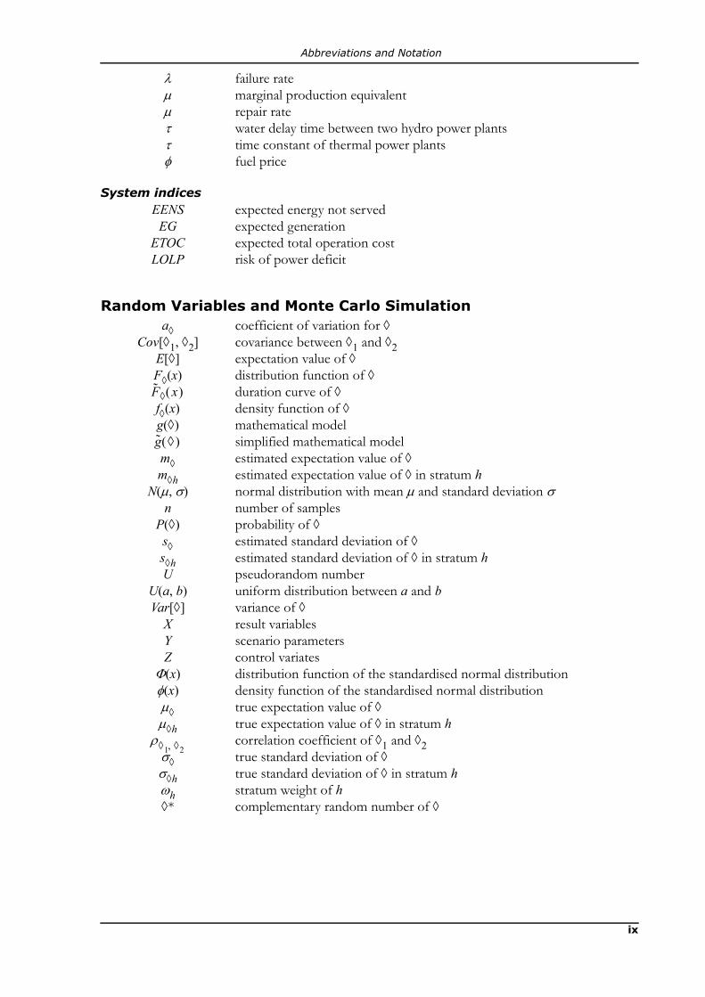
2.2.1 The Ahead TradingBy the ahead trading we refer to all trading which occurs before the actual trading period. Theplayers are assumed to plan so that they buy or produce themselves as much as they sell or con-sume themselves. The players may make a number of different agreements, from long-term con-tracts which are valid for several trading periods, to short-term contracts which only apply to a sin-gle trading period and which typically are made the day before the actual trading period. Bycombining various contracts the players can obtain favourable prices for most of their turnover bylong-term contracts, while they can adept to the circumstances at hand using shorter contracts (cf.figure 2.3). Below we will briefly describe the most common types of ahead trading.
Power Pools
Players who want to trade in a power pool submit purchase and sell bids respectively. These bidscan be designed in different ways. The most simple form of a purchase bid is to specify the highestprice that the player is willing to pay for a certain amount of electric energy during a certain trad-ing period. In a similar manner, a simple sell bid specifies the least price for which the player iswilling to sell a certain amount of electric energy during a certain trading period. Hence, the com-mon purchase and sell bids are valid for one particular trading period. It is also possible to allowbids that are valid for several trading periods. Such bids are called block bids and must be acceptedas a whole. If a player submits a purchase block for 1 000 MWh/h during 5 hours if the price is atmost 20 €/MWh, then this bid will only be accepted if the average electricity price during all fivehours does not exceed 20 €/MWh.
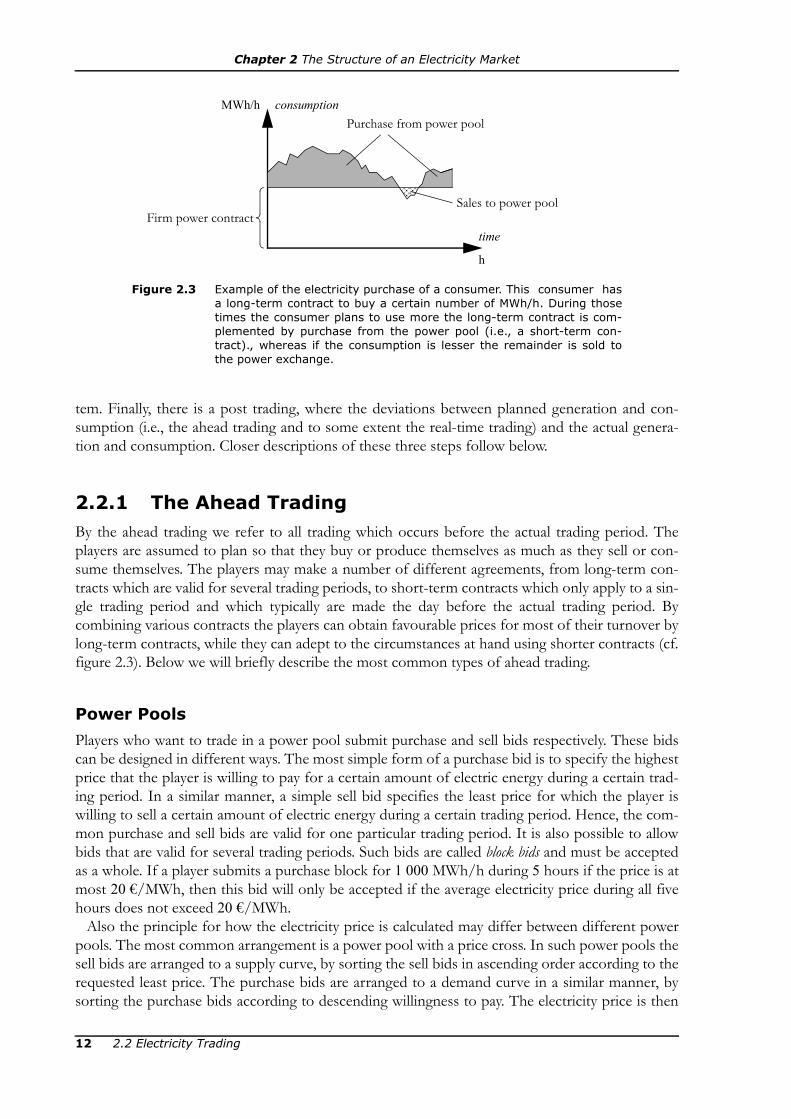
Also the principle for how the electricity price is calculated may differ between different powerpools. The most common arrangement is a power pool with a price cross. In such power pools thesell bids are arranged to a supply curve, by sorting the sell bids in ascending order according to therequested least price. The purchase bids are arranged to a demand curve in a similar manner, bysorting the purchase bids according to descending willingness to pay. The electricity price is then
Figure 2.3 Example of the electricity purchase of a consumer. This consumer hasa long-term contract to buy a certain number of MWh/h. During thosetimes the consumer plans to use more the long-term contract is com-plemented by purchase from the power pool (i.e., a short-term con-tract)., whereas if the consumption is lesser the remainder is sold tothe power exchange.
h
time
MWh/h consumption
Firm power contract
Purchase from power pool
Sales to power pool
12 2.2 Electricity Trading
Chapter 2 The Structure of an Electricity Market
determined by the price cross, i.e., the intersections between the two curves (see figure 2.4). Allbids to the left of the price cross are accepted and they all receive the same electricity price. Thus,all purchase bids where the highest price is higher than the electricity price given for the tradingperiod are accepted, as well as all sell bids where the least price is lesser than the electricity price.Notice that most players receive a price which are more beneficial than the price they were willingto pay and sell for respectively.
Another variant is to have a separate price for each transaction. The power pool lists all submit-ted bids and if a player finds the price appealing they can accept the bid.
Some power pools (for example the Nordic power exchange Nord Pool) have a limitation tohow much may be traded between different parts of the grid. In this case the grid is divided in priceareas. When a player submits a bid to the power pool, they have to specify the price area in whichenergy will be injected or extracted as well as the usual quantity, price and trading period. If thetrading between two areas should exceed the stipulated limitation, then the market is split in multi-ple parts with individual electricity prices for each part.
Bilateral Trading
By bilateral trading we refer to all agreements which are made directly by two players. The bilateraltrading must be reported to the system operator, as it is to be accounted for in the balances of thepost trading market (see section 2.2.3). Bilateral trading is not allowed in centralised electricitymarkets, where all transactions have to pass the power pool.
€/MWh price
Figure 2.4 Principle of a power pool with a price cross.
MWh/hquantity
Purchase bid
Sell bid
Table 2.1 Some examples of power pools.
Power Pool Area Trading period Pricing Bid have to be submitted
European Power Exchange
Germany, Aus-tria 1 hour Price cross No later than 12 a.m. the day before.
Nord Pool ElspotDenmark, Fin-land, Norway, Sweden
1 hour Price cross No later than 12 a.m. the day before.
Nord Pool Elbas Denmark, Fin-land, Sweden 1 hour As in bid
Not earlier than 2 p.m. the day before and no later than one hour before the trading
period.
2.2 Electricity Trading 13

Chapter 2 The Structure of an Electricity Market
Several kinds of contracts are used for bilateral trading. The two most common types of con-tracts are firm power contracts and take-and-pay contracts. Firm power means that a given con-stant power is traded during a given time period. This sort of contract is usually used to cover thebase load. Take-and-pay contracts mean that the buyer can consume as much as he or she wants,up to a certain limit. This type of contract is for example used by regular residential consumers; inthis case the power limit is set by the size of the main fuse.
A bilateral contract also states the electricity price paid by the buyer. The price can either be thesame for the entire duration of the contract (fixed price) or changing over time (variable price). Avariable price can for example be determined by the electricity price at a power exchange plus acertain uplift.
It can be noted that with the exception of a firm power contract with fixed price, a bilateral con-tract will result in some uncertainty. A consumer who is buying electricity at a variable price willnot know the price in advance and a producer who is selling electricity in a take-and-pay contractwill not know the exact sales until after the end of the trading period.
Financial Trading
The financial trading is a trading of various sorts of price insurances. A financial instrument is a bi-lateral agreement between two players. The financial trading is not reported to the system operatorand is not accounted for in the balances of the post trading market. Therefore, financial trading isallowed also in centralised electricity market, although they actually constitute bilateral contracts.
To simplify the financial trading it is possible to introduce different standard contracts. Thesecontracts can then be traded at special markets at a power exchange. Some examples of financialinstruments are options and futures:
•Options. Assume that company B wants to buy a given amount of power during aspecified time period, but the company is not willing to pay more than a certain maxi-mum price. Company B can make an agreement with company A, in which companyA promises to pay the difference if the price on the power exchange is higher than thedesired maximum price. Company B can then buy power from the power exchange.Company B pays company A for the agreement. Company A does not have to be apower company.
•Futures. Company B wants to buy a given amount of power during a specified peri-od to a specified price. Company B agrees with company A for the specified price.Company A then takes risk. Company A obtains the benefit or the loss depending onthe difference between the agreed price and the exchange price. Company A does nothave to be a power company.
2.2.2 Real-time TradingThe real-time trading refers to the trading which occurs during a trading period. The most impor-tant player in the real-time market is the system operator, who has the responsibility to maintainsafe operation of the power system. Therefore, the system operator sometimes has to change theproduction and consumption respectively, and this task is solved by real-time trading. As usual,there are several ways to design the real-time trading. In this compendium we will distinguish be-tween to main types of real-time trading: a real-time balancing market and central dispatch.
Real-time Balancing Market
In a real-time balancing market, the normal condition is that the players themselves decide how
14 2.2 Electricity Trading
Chapter 2 The Structure of an Electricity Market
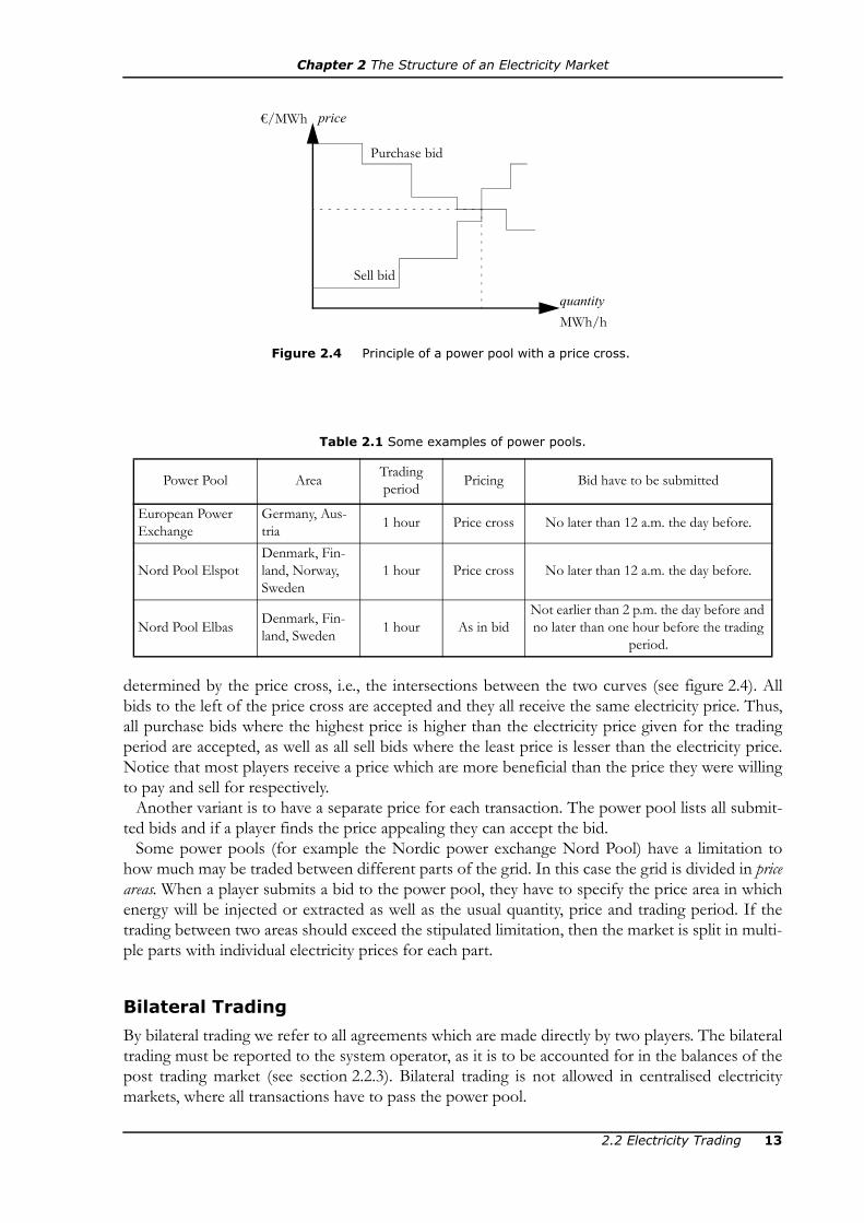
much to produce and consume respectively, but if necessary the system operator can persuade aplayer to change their production or consumption by activating bids which have been submitted tothe real-time balancing market. Two kinds of bids can be submitted to the real-time balancing mar-ket. When down-regulating the system is supplied with less energy than agreed upon in the aheadmarket (thus, a producer carries out down-regulation by reducing the production, whereas a con-
Income
Cost
Figure 2.5 Principles of pricing in a real-time balancing market. In this exam-ple there are seven power plants with increasing variable produc-tion costs. The planned production according to panel a has beensold in the ahead market, resulting in the indicated system price.Each producer now submits bids to the real-time balancing mar-
ket. The power plants which can down-regulate are willing to pay aprice not exceeding their variable production cost (otherwise buy-ing regulating power is a loss). In a similar way, the power plantswhich can up-regulate are only willing to do so if they get paid atleast as much as their variable production costs.In panels b and c regulating power is traded using separate prices
(corresponding to the upper and lower limits respectively of thesubmitted bids). In panel d and e uniform down- and up-regulatingprices are used instead. The first activated bids now receive a morefavourable price than the variable production cost.
MWh/h
production
€/MWh price
MWh/h
production
€/MWh price
MWh/h
production
€/MWh price
MWh/h
production
MWh/h
production
planned
systemprice
a) No regulation.
down-regulation
down-regulation
up-regulation
up-regulation
b) Down-regulation using sepa-rate regulation prices foreach bid.
d) Down-regulation using uni-form prices.
c) Up-regulation using separateregulation prices for each bid.
e) Up-regulation using uniformprices.
up-regulationprice
systemprice
down-regulation price
systemprice
systemprice
systemprice
€/MWh price €/MWh price
2.2 Electricity Trading 15

Chapter 2 The Structure of an Electricity Market
sumer carries out down-regulation by increasing the consumption). Down-regulation means thatthe player buys regulating power from the system operator and a down-regulation bid must there-fore state how much the player can down-regulate (in MW) and the maximal price (in €/MWh)which the player is willing to pay for the regulating power. Similarly, up-regulation means that theplayer sells regulating power to the system operator, i.e., an up-regulation bid states how much theplayer can up-regulate and the minimum price for which the player is willing to sell regulatingpower. Unlike the bids to the ahead market, bids to the real-time balancing market are not just fi-nancial but physical undertakings—the system operator measures generation and load and maycontrol that activated bids really have been carried out within time.
The pricing of the real-time balancing market can either be different for each activated bid orthere may be uniform prices for up- and down-regulation respectively. Separate pricing means thatthose players buying regulating power pay exactly the price they stated in their down-regulationbid and the players selling regulating power get paid as much as they stated in their up-regulationbids. Using this pricing scheme the players will—provided that the competition is good—not beable to make any profits from the real-time trading; for example, a producer will buy regulatingpower at the same price as it would have cost to produce it (cf. figure 2.5b) and will when sellingreceive just as much to cover the production cost (cf. figure 2.5c). Such arrangements are not veryattractive neither for producers nor consumers; it implies that they submits bids out of public dutyor that they are simply forced to submit bids whenever possible. To make a real-time balancingmarket more appealing it is possible to use marginal pricing instead, which means that a down-reg-ulation price is defined, which is equal to the lowest price among the activated down-regulationbids, and an up-regulation price, which is equal to the highest price among the activated up-regula-tion bids. All activated bids will then obtain these regulating prices. Thus, a producer may forexample buy regulating power to a price which is less than what it would have cost to produce thesame amount in an own power plant (cf. figure 2.5d) or may sell regulating power to a price whichis higher than the production cost cf. figure 2.5e).3
Central Dispatch
When central dispatch is applied, the system operator decides how much the other players shouldproduce or consume. The dispatch is based on the bids submitted by the other players during theahead trading. To give the players the possibility of correcting bids based on mistaken forecasts,the players may be allowed to adjust their bids before the real-time trading (to reduce the risk ofmarket manipulation it is possible to require that the players only may change their bids if theyprovide a reasonable motivation). Each trading period is divided in phases (in for example Aus-tralia, five minute intervals are used) and for each phase the system operator performs an eco-nomic dispatch, which means that the system operator solves a short-term planning problembased on the bids of the players. The result of the dispatch states for example how much is to beproduced in each power plant. Separate prices are obtained for each phase (or varying prices fordifferent parts of the grid if the economic dispatch accounts for losses and/or transmission limita-tions); these prices are referred to as real-time prices.
2.2.3 Post TradingAs noted earlier, the objective of the electricity trading is to assure that somebody is paying for the
3. It is actually possible to combine the two pricing schemes. An example of this is the Nordic electricity market,where the regulating bids activated to maintain balance between production and consumption are paid uniformup- and down-regulation prices, whereas those bids activated to prevent a part of the grid to be overloaded (so-called counter trading) receive separate prices.
16 2.2 Electricity Trading

Chapter 2 The Structure of an Electricity Market
energy transferred in the power system. When a trading period is ended the system operator cancompile how much the balance responsible and his or her clients have actually produced and con-sumed, as well as how much they have bought or sold in the ahead and real-time markets. This willalmost certainly result in a deviation between supplied and extracted energy. The purpose of thepost trading is to settle these deviations.
All balance responsible players having an imbalance have to trade in the post market in order toachieve balance. Players having positive imbalances (i.e., they have supplied more energy than theyhave extracted) sell imbalance power to the system operator. If there is a negative imbalanceinstead then the player has to buy imbalance power from the system operator.
The price of the imbalance power is generally related to the prices used during the real-time trad-ing and as usual there are several variants. The question is partly whether average pricing is used(as for example in Denmark, England-Wales and Spain) or marginal pricing (as for example inAustralia, Finland, Norway and Sweden), and partly whether or not separate prices are used forbuying and selling imbalance power. A one-price system means that all imbalance power is boughtand sold for the same price (this is the case in for example Australia, Norway, Spain and Ger-many), whereas a two-price system means that there are separate prices for negative and positiveimbalances respectively (this is the case in for example Denmark, Finland, Sweden and England-Wales).
An overview of the principles for one-price and two-price systems is given in figure 2.6. If thereal-time trading has required both up- and down-regulations then it must first be decided thedirection of the net regulation during the trading period; if the system operator has bought moreregulating power than they have sold then the trading period counts as up-regulation and viceversa. In a one-price system the up-regulation price is used for all imbalance power during up-reg-ulation periods (a) and the down-regulation price is used during down-regulation periods(figure 2.6b). If the real-time market uses central dispatch rather than a real-time balancing market,the real-time price is used instead of up- and down-regulation prices.
The two-price system means that a less favourable price is given to those players who areassumed to be the cause of the activation of regulating bids. During an up-regulation period thoseplayers who have not supplied enough energy, i.e., which have negative imbalances, must pay theup-regulation price (which is higher than the price in the ahead market), while the players havingpositive balance receive the same price as in the ahead market (figure 2.6c). During down-regula-tion on the other hand, those players having positive imbalance are assumed to have caused theneed for regulation and therefore are getting paid the down-regulation price (which is less than theahead market price), while the other players receive the same price as in the ahead market(figure 2.6d). This approach can also be applied to real-time prices originating from a central dis-patch; if the real-time price is higher than the ahead market price then there has been an up-regu-lation period and vice versa.
Using a one-price system a balance responsible having an imbalance in “the right direction” (i.e.,positive imbalance when the system has a net up-regulation and negative imbalance when the sys-tem has a net down-regulation) may buy or sell imbalance power to a price more favourable thanin the ahead market, which means that there in some cases will be profitable to have an imbalance.Thus, the one-price system introduces a possibility to intentionally obtain an imbalance, but it ishard to see how a player systematically could take advantage of this possibility. However, the one-price system means that the costs decrease for those being balance responsible of unpredictableproduction or consumption, because the cost of the occasions when the player has an imbalancein “the wrong direction” is to some extent compensated by the income of the occasions when theplayer has an imbalances in “the right direction”. In a two-price system it is never possible to makeany profits from an imbalance, which results in higher costs for the balance responsible players,who accordingly can be assumed to feel more pressure to keep their own balance in every tradingperiod.
2.2 Electricity Trading 17

Chapter 2 The Structure of an Electricity Market
Example 2.1 (trading of imbalance power): Consider two balance responsi-bility players in an electricity market. Player A is both acting as a producer and as aretailer and must plan generation and trading at the power pool to cover the expectedload of the consumers during the hour. Player B is a pure producer. Table 2.2 showsthe plans of the two players for the trading period between 10 am and 11 am.At 10:15 a power plant generating 200 MW belonging to player A fails. To at leastpartly compensate the lost generation A increases the generation in their hydro powerplants by 180 MW at 10:30.Player B submitted a sell bid to the power pool for a power plant having an operation
€/MWh price
MWh/h
imbalance
+–
a) Single-price system during anup-regulation period.
b) Single-price system during adown-regulation period.
c) Two-price system during an up-regulation period.
d) Two-price system during adown-regulation period.
e) Mixed price system during anup-regulation period. The costof positive imbalance is themean value of the system priceand the up-regulation price.
f) Two-price system with dead-band during a down-regulationperiod.
Figure 2.6 Different pricing schemes for the post market. Players have posi-tive imbalance when supplying more energy during the tradingperiod than they have extracted. The system price refers to theelectricity price in the ahead market, whereas up- and down-regu-lation prices refer to the prices of the real-time balancing market(corresponding to the real-time price if central dispatch is used).
up-regulation price
down-regulation price
up-regulationprice
systemprice
up-regulationprice
€/MWh price
MWh/h
imbalance
+–
€/MWh price
MWh/h
imbalance
+–
€/MWh price
MWh/h
imbalance
+–
€/MWh price
MWh/h
imbalance
+–
€/MWh price
MWh/h
imbalance
+–
systemprice
systemprice
down-regulation price
down-regulation price
18 2.2 Electricity Trading
Chapter 2 The Structure of an Electricity Market
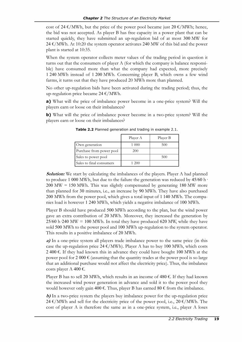
cost of 24 €/MWh, but the price of the power pool became just 20 €/MWh; hence,the bid was not accepted. As player B has free capacity in a power plant that can bestarted quickly, they have submitted an up-regulation bid of at most 300 MW for24 €/MWh. At 10:20 the system operator activates 240 MW of this bid and the powerplant is started at 10:35.When the system operator collects meter values of the trading period in question itturns out that the consumers of player A (for which the company is balance responsi-ble) have consumed more than what the company had expected, more precisely1 240 MWh instead of 1 200 MWh. Concerning player B, which owns a few windfarms, it turns out that they have produced 20 MWh more than planned.No other up-regulation bids have been activated during the trading period; thus, theup-regulation price became 24 €/MWh. a) What will the price of imbalance power become in a one-price system? Will theplayers earn or loose on their imbalances?b) What will the price of imbalance power become in a two-price system? Will theplayers earn or loose on their imbalances?
Solution: We start by calculating the imbalances of the players. Player A had plannedto produce 1 000 MWh, but due to the failure the generation was reduced by 45/60 h·200 MW = 150 MWh. This was slightly compensated by generating 180 MW morethan planned for 30 minutes, i.e., an increase by 90 MWh. They have also purchased200 MWh from the power pool, which gives a total input of 1 140 MWh. The compa-nies load is however 1 240 MWh, which yields a negative imbalance of 100 MWh.Player B should have produced 500 MWh according to the plan, but the wind powergave an extra contribution of 20 MWh. Moreover, they increased the generation by25/60 h·240 MW = 100 MWh. In total they have produced 620 MW, while they havesold 500 MWh to the power pool and 100 MWh up-regulation to the system operator.This results in a positive imbalance of 20 MWh.a) In a one-price system all players trade imbalance power to the same price (in thiscase the up-regulation price 24 €/MWh). Player A has to buy 100 MWh, which costs2 400 €. If they had known this in advance they could have bought 100 MWh at thepower pool for 2 000 € (assuming that the quantity trades at the power pool is so largethat an additional purchase would not affect the electricity price). Thus, the imbalancecosts player A 400 €.Player B has to sell 20 MWh, which results in an income of 480 €. If they had knownthe increased wind power generation in advance and sold it to the power pool theywould however only gain 400 €. Thus, player B has earned 80 € from the imbalance.b) In a two-price system the players buy imbalance power for the up-regulation price24 €/MWh and sell for the electricity price of the power pool, i.e., 20 €/MWh. Thecost of player A is therefore the same as in a one-price system, i.e., player A loses
Table 2.2 Planned generation and trading in example 2.1.
Player A Player B
Own generation 1 000 500Purchase from power pool 200Sales to power pool 500Sales to final consumers 1 200
2.2 Electricity Trading 19

Chapter 2 The Structure of an Electricity Market
400 € on the imbalance. For player B the income of the sold imbalance power isdecreased to 400 €, which means that player B neither gains nor loses from the imbal-ance.
Finally, it can be mentioned that there are some other variants of pricing imbalance power. Itmight for example be desirable to compromise between a wish to motivate the balance responsibleplayers to keep their balance and a wish to not disadvantage players having difficulties predictingor regulating production and consumption. Such a compromise is to use a two-price system,where those players having imbalance in “the right direction” will not receive a price as favourableas the corresponding regulating price, but still better than the price of the ahead market (for exam-ple a mixed price system as in figure 2.6e). It is also possible to refrain from punishing lesserimbalances by an unfavourable price (so-called dead-band; seefigure 2.6f).
EXERCISES2.1 Which are the responsibilities of the system operator?2.2 What does it mean to be balance responsible?2.3 What are the responsibilities of a grid owner?2.4 How is a vertically integrated electricity market organised?2.5 How is a centralised electricity market organised?2.6 How is a bilateral electricity market organised?2.7 What does ahead trading refer to?2.8 How is electricity traded in a power exchange?2.9 What is a block bid?2.10 What is a firm power contract?2.11 What is a take-and-pay contract?2.12 What does real-time trading refer to?2.13 What does an up-regulation bid mean?2.14 What does a down-regulation bid mean?2.15 What does post trading refer to?
FURTHER READING• S. Stoft, Power System Economics, IEEE Press, 2002. — Basic textbook on electricity markets.• I. Wrangensteen, Power System Economics – the Nordic Electricity Market, Tapir Academic Press, Trond-
heim 2007. — Basic textbook with focus on the Nordic electricity market.• “Balance Responsible Agreement”, Svenska kraftnät. [Available at http://www.svk.se] — The regu-
lation for balance responsible players in Sweden.• “EPEX Spot Market Rules and Regulations”, European Power Exchange, November 2011. [Availa-
ble at http://www.epexspot.com] — The regulation for the European Power Exchange.• “System Operation Agreement 2006-06-13”, Nordel, 2006. [Available at https://www.entsoe.eu]
— The contract which regulates the cooperation between the Nordic system operators.• “Trade at NPS”, Nord Pool Spot. [Available at http://www.npspot.com/trading/] — Description of
the Nordic power exchange Nord Pool.• “Trade at Nord Pool ASA’s Financial Market”, Nord Pool, March 2010. [Available at http://
www.nasdaqomxcommodities.com/trading/] — Description of the Nordic power exchange Nord Pool.
20 Exercises

Chapter 3
ELECTRICITY PRICING
This chapter describes a simple model for electricity pricing. The objective of the model is to pro-vide a basic understanding on the factors which influence the electricity price and the relative im-portance of individual factors.
3.1 PRICINGAs for any good which is traded in a free market environment, the price of electricity will be set bysupply and demand. Assume that there is a number of producers1 and it is known how much theycan produce of a particular good. Given a number of producers, the price for which they are will-ing to sell a particular good and which production costs they have. It is then possible to arrange asupply curve, which will show the total production of the good for a given price. In the same wayit is possible to create a demand curve, which shows the total consumption for a given price.Figure 3.1 shows examples of such curves.
The market price is set by the intersection of the supply and demand curves. It can be shownthat this trading maximises the total surplus, i.e., this is the most efficient solution from the soci-ety’s point of view. It should be noted that this is stable equilibrium point, because no player cangain anything from trying to deviate from the market price. Consider for example a producerwhich can not sell his or her production, because the producer is requiring a higher price than themarket price. No consumer will be interested in buying from this producer, as they can buy thesame good from some other producer to the market price instead. Admittedly, there are also someconsumers who are not supplied at all in the current equilibrium, but they are on the other handnot even willing to pay the market price. The only thing that our example producer can do to getmore customers is to reduce the price. This is only profitable if the marginal production cost, i.e.,the variable manufacturing cost, is less than the market price.
If we instead consider a producer who is selling the good, this producer could increase his or herby demanding a higher price. However, this is only possible if the wanted price not is higher thanthe market price. If the producer is trying to exceed this limit then the consumers instead will turnto the least expensive producer having free production capacity. This does of course presupposethat there are a lot of producers in the market and that the marginal cost is not showing too largedifferences; when there will always be a producer having unused production capacity available woa marginal cost which is only slightly higher than the market price.
1.We assume that all producers manufacture equivalent products.
3.1 Pricing 21
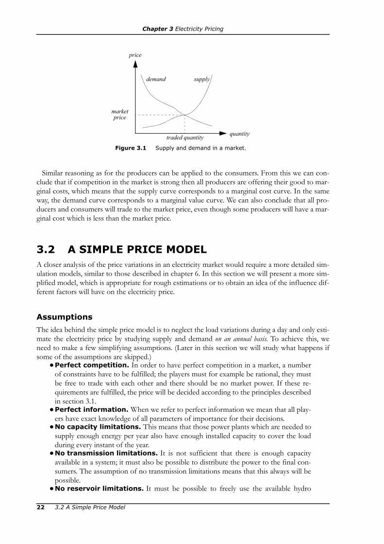
Chapter 3 Electricity Pricing
Similar reasoning as for the producers can be applied to the consumers. From this we can con-clude that if competition in the market is strong then all producers are offering their good to mar-ginal costs, which means that the supply curve corresponds to a marginal cost curve. In the sameway, the demand curve corresponds to a marginal value curve. We can also conclude that all pro-ducers and consumers will trade to the market price, even though some producers will have a mar-ginal cost which is less than the market price.
3.2 A SIMPLE PRICE MODELA closer analysis of the price variations in an electricity market would require a more detailed sim-ulation models, similar to those described in chapter 6. In this section we will present a more sim-plified model, which is appropriate for rough estimations or to obtain an idea of the influence dif-ferent factors will have on the electricity price.
Assumptions
The idea behind the simple price model is to neglect the load variations during a day and only esti-mate the electricity price by studying supply and demand on an annual basis. To achieve this, weneed to make a few simplifying assumptions. (Later in this section we will study what happens ifsome of the assumptions are skipped.)
•Perfect competition. In order to have perfect competition in a market, a numberof constraints have to be fulfilled; the players must for example be rational, they mustbe free to trade with each other and there should be no market power. If these re-quirements are fulfilled, the price will be decided according to the principles describedin section 3.1.
•Perfect information. When we refer to perfect information we mean that all play-ers have exact knowledge of all parameters of importance for their decisions.
•No capacity limitations. This means that those power plants which are needed tosupply enough energy per year also have enough installed capacity to cover the loadduring every instant of the year.
•No transmission limitations. It is not sufficient that there is enough capacityavailable in a system; it must also be possible to distribute the power to the final con-sumers. The assumption of no transmission limitations means that this always will bepossible.
•No reservoir limitations. It must be possible to freely use the available hydro
price
quantity
demand supply
Figure 3.1 Supply and demand in a market.
marketprice
traded quantity
22 3.2 A Simple Price Model

Chapter 3 Electricity Pricing
power energy during the year. To make this possible there must not be any reservoirlimitations, which prevents us from storing enough hydro energy from one part of theyear to another.
•The load is not price sensitive. If the load is not price elastic then the demandcurve is corresponding to a vertical line at the quantity corresponding to the annualload. On most markets it is reasonable to simplify the demand curve in this way, be-cause most consumers have take-and-pay contracts2 where they pay a fixed price perkWh. These consumers have no reason to change their electricity consumption even ifthe electricity price is increasing.
The supply curve can be compiled by combining the variable operation cost of the power plantsand the potential energy generation in each power source. The average electricity price during ayear (or any other longer time period) can then be estimated by determining the intersection of thesupply and demand, according to the pricing theory described above.
Example 3.1 (price in a simple electricity market): Assume that we have apower system supplied by hydro power and coal condensing. The potential hydropower generation is limited by the inflow, which is 60 TWh/year. The potential of thecoal condensing units is 30 TWh/year. The load is 75 TWh/year. The variable opera-tion costs are assumed to be 30-60 SEK/MWh for hydro power and 160-180 SEK/MWh for coal condensing. The operation costs are assumed to be linearwithin the stated intervals, i.e., if the generation is equal to zero then the price is equalto the lower value, and for maximal generation the price is equal to the higher value.Assume perfect competition, perfect information and that there are neither anycapacity, transmission nor reservoir limitations. Which electricity price will we have inthis system? Also calculate the difference between variable operation cost and totalincome of the power producers.Solution: The supply curve of this system is shown in figure 3.2. If the annual con-sumption would have been less than 60 TWh then the system could have been sup-plied solely by hydro power. The assumption of not having any capacity, transmissionor reservoir limits makes it possible to distribute the available hydro energy during theyear so that the whole load can be covered. If the price would be different during dif-ferent parts of the year, the hydro power producers could earn money by saving waterin the reservoirs from low price periods to high price periods. This would result in
2.See section 2.2.1.
10 TWh/yearGtot
150
100
50
200
20 30 40 50 60 70 80 90 100
Figure 3.2 Supply and demand of the electricity market in example 3.1.
DSEK/MWh λ
3.2 A Simple Price Model 23

Chapter 3 Electricity Pricing
increasing prices during the lower price periods and decreasing prices in the high priceperiods, until the price has been levelled out between the different parts of the year.For a load which is larger than 60 TWh some of the coal condensing units will beneeded. When the load is 75 TWh all coal condensing up to the marginal cost170 SEK/MWh. The assumption of perfect information means that the hydro powerowners are aware of this and will demand the price170 SEK/MWh for their electricitygeneration too. The assumption of perfect competition means that nobody will beable to sell power to a price higher than 170 SEK/MWh, because then they will loosetheir sales to somebody who offers to sell for 170 SEK/MWh.The total variable operation cost in this example is
PC = = 5 175 MSEK,
while the income isPV = 75 · 170 = 12 750 MSEK,
i.e., the total producers’ surplus is 12 750 – 5 175 = 7 575 MSEK. It should howeverbe noted that this surplus is not pure profit, but should also cover fixed costs as capi-tal cost and labour costs.
Price Sensitive Load
The simple price model does not change much if we release the assumption that the load is notprice sensitive; we will still look for the intersection of the supply and demand curves.
Example 3.2 (price sensitive load). Consider the same electricity market as inexample 3.1, but assume that part of the load is not price sensitive and a part of it thatis price sensitive. The price insensitive load is 72 TWh/year, while the price sensitiveload is 10 TWh if the price does not exceed 100 SEK/MWh and will then decreaselinearly until the price reaches 200 SEK/MWh; at this price level the elastic consump-tion has decreased to zero. Assume perfect competition, perfect information and thatthere are neither any capacity, transmission nor reservoir limitations. Which electricityprice will we have in this system? How large will the total consumption become?Solution: The supply and demand curves of this system are shown in figure 3.3. The
60 30 60+( )2
----------------------- 15 160 170+( )2
-----------------------------⋅+⋅
Figure 3.3 Supply and demand of the electricity market in example 3.2.
D
10 TWh/yearGtot
150
100
50
200
20 30 40 50 60 70 80 90 100
SEK/MWh λ
24 3.2 A Simple Price Model
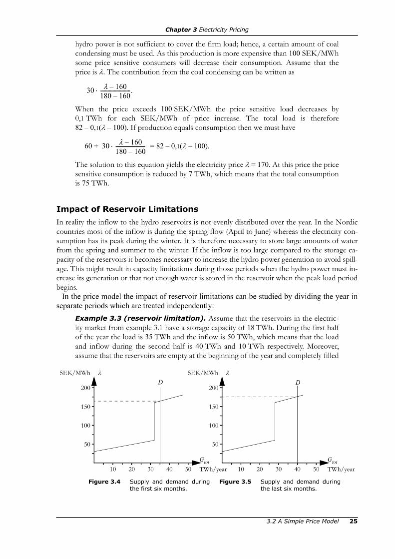
Chapter 3 Electricity Pricing
hydro power is not sufficient to cover the firm load; hence, a certain amount of coalcondensing must be used. As this production is more expensive than 100 SEK/MWhsome price sensitive consumers will decrease their consumption. Assume that theprice is λ. The contribution from the coal condensing can be written as
When the price exceeds 100 SEK/MWh the price sensitive load decreases by0,1 TWh for each SEK/MWh of price increase. The total load is therefore82 – 0,1(λ – 100). If production equals consumption then we must have
60 + = 82 – 0,1(λ – 100).
The solution to this equation yields the electricity price λ = 170. At this price the pricesensitive consumption is reduced by 7 TWh, which means that the total consumptionis 75 TWh.
Impact of Reservoir Limitations
In reality the inflow to the hydro reservoirs is not evenly distributed over the year. In the Nordiccountries most of the inflow is during the spring flow (April to June) whereas the electricity con-sumption has its peak during the winter. It is therefore necessary to store large amounts of waterfrom the spring and summer to the winter. If the inflow is too large compared to the storage ca-pacity of the reservoirs it becomes necessary to increase the hydro power generation to avoid spill-age. This might result in capacity limitations during those periods when the hydro power must in-crease its generation or that not enough water is stored in the reservoir when the peak load periodbegins.
In the price model the impact of reservoir limitations can be studied by dividing the year inseparate periods which are treated independently:
Example 3.3 (reservoir limitation). Assume that the reservoirs in the electric-ity market from example 3.1 have a storage capacity of 18 TWh. During the first halfof the year the load is 35 TWh and the inflow is 50 TWh, which means that the loadand inflow during the second half is 40 TWh and 10 TWh respectively. Moreover,assume that the reservoirs are empty at the beginning of the year and completely filled
30 λ 160–180 160–------------------------ .⋅
30 λ 160–180 160–------------------------⋅
Figure 3.4 Supply and demand duringthe first six months.
Figure 3.5 Supply and demand duringthe last six months.
D D
10 TWh/yearGtot
150
100
50
200
20 30 40 50
SEK/MWh λ
10 TWh/yearGtot
150
100
50
200
20 30 40 50
SEK/MWh λ
3.2 A Simple Price Model 25

Chapter 3 Electricity Pricing
after the first half of the year. Determine the electricity price during the year. The coalcondensing potential can be assumed to be evenly distributed over the year.Solution: During the first half of the year it is possible to generate 32 TWh of hydropower, i.e., the inflow during the period minus the water which is stored in the reser-voir after six months. Further, it is possible to use half of the coal condensing poten-tial. The resulting marginal cost curve is shown in figure 3.4. The electricity pricebecomes 164 SEK/MWh.During the second half of the year only 18 + 10 = 28 TWh hydro energy is available.Together with half of the coal condensing potential we get the marginal cost curveshown in figure 3.5. The electricity price during the second half of the year is176 SEK/MWh.Notice that the electricity price was higher in the period after the reservoirs werefilled. If the price would have been lower during the second half of the year then itwould have been profitable to store less water for that part of the year and use it tolower the price during the first six months instead. This way it would have been possi-ble to “move” water from the second half of the year to the first until the price differ-ence had been levelled out.
Impact of Forecast Uncertainties
In reality it is impossible to have perfect information about all factors affecting the operation ofthe power system. This is primarily a problem in power system with a large share of dispatchablehydro power, because long-term hydro power planning require knowledge about inflow, availabil-ity in thermal power plants and load in order to utilise the hydro energy in an optimal manner. Allthese quantities must however be estimated by forecasts.
One of the most uncertain forecasts is the annual inflow. If it is believed that the inflow will behigh then the need for thermal power will decrease and the marginal cost will be relatively low. If iton the other hand is believed that the inflow will be low then higher marginal costs will beexpected. This principle is illustrated in the following example:
Example 3.4 (uncertain inflow forecasts): Assume that an electricity markethas a potential of 30 TWh/year in the coal condensing units. There is also dispatcha-ble hydro power in the system, but the information about the inflow for the comingtwelve months are changing according to figure 3.6, i.e., at the beginning of the yearthe inflow is expected to be 60 TWh, but due to increased precipitation during the
5 weektime of the year
70
60
50
TWh/year V
10 15 20 25 30 35 40 45 50
Figure 3.6 Forecasted hydro power potential for the next twelve months inexample 3.4.
26 3.2 A Simple Price Model

Chapter 3 Electricity Pricing
spring the expectations are increased to 69 TWh after six months. In the autumn, theinflow is however far less than expected, which causes the expectations to decreasecontinuously to 57 TWh at the end of the year. The load is 75 TWh/year. The opera-tion costs are assumed to be linear within the stated intervals, i.e., if the generation isequal to zero then the price is equal to the lower value, and for maximal generationthe price is equal to the higher value. Assume perfect competition, perfect informa-tion about everything except the inflow and that there are neither any capacity, trans-mission nor reservoir limitations. How will the electricity price develop during thestudied year?Solution: The conditions in the first week of the year are exactly the same as inexample 3.1; hence, the electricity price is the same, i.e., 170 SEK/MWh. It can benoticed that this conclusion is based on the assumption that all players have the sameforecast about the inflow.After six months the players of the market believe that the inflow will be 69 TWh thenext twelve months. The supply curve in this case is shown in figure 3.7. The resultfrom example 3.1is also shown in the figure by a dotted line. The difference is that theincreased amount of hydro energy has shifted the coal condensing part of the supplycurve rightwards. The same reasoning as in example 3.1 yields that the electricity priceis 164 SEK/MWh.As the marginal cost of the coal condensing units is a linear function the electricityprice λ will be a linear function of the expected hydro power generation the nexttwelve months:
λ = 160 + = 210 – SEK/MWh.
This function is of course only valid when the electricity consumption is75 TWh/year and the marginal cost is set by the coal condensing units, i.e., when 45 ≤V ≤ 75. Using this relation and the given the expected hydro power potential accord-ing to figure 3.6 the electricity price must vary as shown in figure 3.8.
Market Power
Market power arises when one or more players have such a large market share that they can affect
Figure 3.7 Supply and demand after six months in example 3.4.
D
10 TWh/yearGtot
150
100
50
200
20 30 40 50 60 70 80 90 100
SEK/MWh λ
180 160–30
------------------------ 75 V–( ) 23---V
3.2 A Simple Price Model 27

Chapter 3 Electricity Pricing
the market price. A producer having market power can increase his or her profit by decreasing theelectricity generation. They can also force competitors to leave the market, by selling power to lessthan marginal cost and by that means lower the electricity price to a level where the competitor isno longer profitable. In other words, the producer is willing to accept a limited loss of profits inorder to get rid of a competitor and increase the profits in a long-term perspective.
A player with market power is often referred to as a price setter, unlike other players which are pricetakers. The difference between a price setter and a price taker is illustrated in figure 3.9. A pricetaker has such a small production capacity compared to the total turn-over of the market that theactions of the producer do not affect the demand, as shown in figure 3.9a. This producer will max-imise his or her profit by producing as much us possible as long as the marginal cost (i.e., the sup-ply curve) is less than the willingness to pay of the consumers (i.e., the demand curve). If all pro-ducers as producing so much that their marginal costs are equal to the marginal benefit, then themarket has reached the equilibrium point which maximised the total surplus.
However, if the producer is a price setter the situation is different. A price setter has such a largeshare of the market that his or her actions affect the price. In figure 3.9b we can see that if the pro-ducer decreases the production from q to q* then the profits are decreased by an amount corre-sponding to the shaded area B, but on the other hand the price is increasing, which means that theincome of the remaining sales increase by an amount equal to the shaded area A. If A is larger thanB then it would be profitable to decrease the production, even though the producer’s marginalcost is less than the market price. It must be noticed that the reduced production only is profitable
Figure 3.8 Development of the electricity price during theyear in example 3.4.
5 weektine of the year
180
170
160
SEK/MWh λ
10 15 20 25 30 35 40 45 50
price
quantity
price
quantity
demand
supply
demand supply
AB
qq*qa) Company specific supply and demand
of a price taker.b) Company specific supply and demand
of a price setter.
Figure 3.9 Illustration of the difference between a price taker and a price setter.
28 3.2 A Simple Price Model

Chapter 3 Electricity Pricing
for the price setter, but not for the society as a whole!Since market power is not good for the total surplus, the authorities usually try to limit market
power by legislation. This is however in many cases difficult, as it can be hard to prove that a com-pany is misusing its market power.
Example 3.5 (one player with market power): Assume that there is an elec-tricity market with one large producer, AB Kraftjätten, which can generate up to60 TWh/year at the cost 40 SEK/MWh. The remaining producers all have very smallcapacity compared to the turn-over of the market. Their marginal costs vary between40 SEK/MWh and 200 SEK/MWh, as shown in figure 3.10.During a certain year the demand is 80 TWh and we can assume that the load is notprice sensitive. Assume perfect information and that there are neither any capacity,transmission nor reservoir limitations. Which electricity price would we have if there isperfect competition? What would the electricity price be if AB Kraftjätten chooses toutilise its position as a price setter?Solution: In a perfect market the price would be set by the intersection of supply anddemand, i.e., 120 SEK/MWh. At this point Kraftjätten AB would generate its fullpotential. By reducing the generation the company can however increase the electric-
10 TWh/yearGtot
150
100
50
200
20 30 40 50 60 70 80 90 100
Figure 3.10 Supply and demand of the electricity market in example 3.5.
DSEK/MWh λ
10 TWhG
6 000
4 000
2 000
8 000
MSEK PS
20 30 40 50 60
Figure 3.11 The surplus of AB Kraftjätten as a function ofchosen annual generation.
Illicitarea
3.2 A Simple Price Model 29
Chapter 3 Electricity Pricing
ity price. For each TWh of reduced generation the electricity price will increase by4 SEK/MWh, i.e., we can express the electricity price as
λ(G) = 120 – 4(G – 60) = 360 – 4G,
where G is the annual generation of AB Kraftjätten. This relation is only valid when40 ≤ G ≤ 60; if the generation is lower than 40 TWh then there would be an energydeficit, which hardly would be tolerated by the system operator. In the allowed inter-val the surplus of AB Kraftjätten (i.e., income minus costs) by
PS(G) = G·λ(G) – 40G = 320G – 4G2.This function is shown in figure 3.11. As can be seen, the company is maximising itssurplus by decreasing the annual generation to 40 TWh. Such a large reduction mayhowever draw attention from the authorities, which for example could force the com-pany to be split in several smaller companies to increase competition. In the long runit might therefore be profitable for AB Kraftjätten to just reduce the generation a lit-tle, which will not give the same profits, but will allow the company to keep its posi-tion as a price setter.
EXERCISES3.1 Determine the electricity price in a small electricity market, where the annual con-
sumption is 72.5 TWh/year. The power is generated in nuclear power plants having avariable operation cost between 100 and 120 ¤/MWh (annual potential 40 TWh) andcombined heat and power plants with a variable operation cost between 80 and150 ¤/MWh (annual potential 35 TWh). The operation costs are assumed to be linearwithin the stated intervals, i.e., if the generation is equal to zero then the price is equalto the lower value, and for maximal generation the price is equal to the higher value.Assume perfect competition, perfect information and that there are neither anycapacity nor transmission limitations.
3.2 What will happen to the electricity price of the market in the previous exercise if10 TWh of the nuclear generation is replaced by 10 TWh wind power?
3.3 Figure 3.12 shows supply and demand for a certain electricity market.a) What will the electricity price become in this electricity market if we assume per-fect competition, perfect information and that there are neither transmission-, reser-voir nor capacity limitations?b) Assume that a certain company owns all hydro power plants in this electricity mar-ket and have fixed costs of 100 M¤/year. How large is the profit of the company?
3.4 Consider a simplified model of the electricity market in Land. Data for the powerplants are given in table 3.1. The operation costs are assumed to be linear within thestated intervals, i.e., if the generation is equal to zero then the price is equal to thelower value, and for maximal generation the price is equal to the higher value. a) Assume that the electricity market in Land has perfect competition, all players haveperfect information, and there are neither transmission nor capacity limitations. Howlarge is the electricity consumption in Land if the electricity price during a certain yearis 220 ¤/MWh?b) AB Vattenkraft owns hydro power plants with a combined production capacity of10 TWh/year. The fixed costs of the company are 650 M¤/year. How large are the
30 Exercises
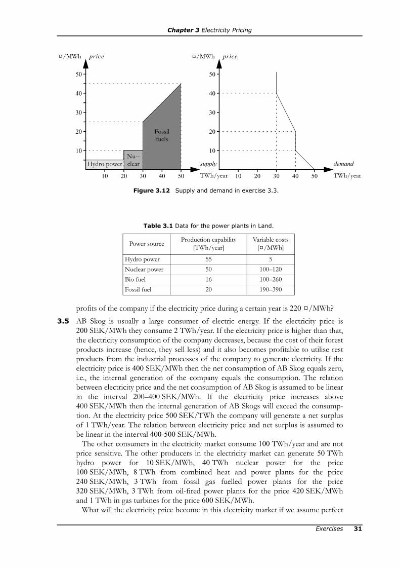
Chapter 3 Electricity Pricing
profits of the company if the electricity price during a certain year is 220 ¤/MWh?3.5 AB Skog is usually a large consumer of electric energy. If the electricity price is
200 SEK/MWh they consume 2 TWh/year. If the electricity price is higher than that,the electricity consumption of the company decreases, because the cost of their forestproducts increase (hence, they sell less) and it also becomes profitable to utilise restproducts from the industrial processes of the company to generate electricity. If theelectricity price is 400 SEK/MWh then the net consumption of AB Skog equals zero,i.e., the internal generation of the company equals the consumption. The relationbetween electricity price and the net consumption of AB Skog is assumed to be linearin the interval 200–400 SEK/MWh. If the electricity price increases above400 SEK/MWh then the internal generation of AB Skogs will exceed the consump-tion. At the electricity price 500 SEK/TWh the company will generate a net surplusof 1 TWh/year. The relation between electricity price and net surplus is assumed tobe linear in the interval 400-500 SEK/MWh.
The other consumers in the electricity market consume 100 TWh/year and are notprice sensitive. The other producers in the electricity market can generate 50 TWhhydro power for 10 SEK/MWh, 40 TWh nuclear power for the price100 SEK/MWh, 8 TWh from combined heat and power plants for the price240 SEK/MWh, 3 TWh from fossil gas fuelled power plants for the price320 SEK/MWh, 3 TWh from oil-fired power plants for the price 420 SEK/MWhand 1 TWh in gas turbines for the price 600 SEK/MWh.
What will the electricity price become in this electricity market if we assume perfect
Figure 3.12 Supply and demand in exercise 3.3.
TWh/year
supply
5040302010
¤/MWh price
50
40
30
10
20
TWh/year
demand
5040302010
¤/MWh price
50
40
30
10
20
Hydro powerNu--clear
Fossilfuels
Table 3.1 Data for the power plants in Land.
Power source Production capability [TWh/year]
Variable costs [¤/MWh]
Hydro power 55 5Nuclear power 50 100–120Bio fuel 16 100–260Fossil fuel 20 190–390
Exercises 31

Chapter 3 Electricity Pricing
competition, perfect information and that there are neither transmission-, reservoirnor capacity limitations?
3.6 Table 3.2 shows the available generation resources, marginal generation costs andannual consumption in the Nordic countries during year 2000. The operation costsare assumed to be linear within the stated intervals, i.e., if the generation is equal tozero then the price is equal to the lower value, and for maximal generation the price isequal to the higher value. Assume perfect competition, perfect information and thatthere are neither any capacity, transmission nor reservoir limitations. Finland imports4 TWh from Russia, Denmark exports 5 TWh to Germany, Sweden exports 0.5 TWhto Germany as well as 0.5 TWh to Poland.
a) Estimate the electricity price.b) Estimate the trading between the Nordic countries.c) How would the electricity price be affected if there is a reservoir limitation so thatthe reservoirs are filled on July 31? Everything else is assumed to be the same asabove. No numerical values have to be calculated; just describe the trend.
3.7 Consider the Nordic electricity market model in exercise 3.6. Assume that all play-ers—except one—are small enough to be considered as price-takers. Investigatewhether or not it is profitable to exercise market power for the large company in thefollowing two cases:a) Assume that one company, Voimajättiäs OY., owns all Finnish hydro power plantsand nuclear power plants.b) Assume that one company, Kraftjätten AB, owns all Swedish hydro power plantsand nuclear power plants.
3.8 An external cost is a cost which is due to the production or consumption of a good,which is neither paid by the producer nor the consumer, but paid by a third partyinstead. Emission of dangerous pollutants from combustion of fossil fuels is an exam-ple of an external cost in an electricity market.
The maximal annual production of the power plants in Land are shown in table 3.3below. The variable production costs are assumed to be linear in the intervals, i.e., theproduction is zero if the price is on the lower price level and the production is maxi-mal at the higher price level. The annual consumption in Land is 100 TWh. a) Assume perfect competition, perfect information and that there are neither capac-ity, transmission nor reservoir limitations. Moreover, assume that the cost of the emis-sions is an external cost. Estimate the electricity price in Land.
Table 3.2 Available generation resources and annual consumption.
Power sourceProduction capability [TWh/year] Cost
[SEK/MWh]Sweden Norway Finland Denmark
Hydro power 78 142 14 - 40Wind power 0.5 0 0 4 20Nuclear power 55 - 21.5 - 50–75Industrial backpressure 5 - 13 2 40–100Comb. heat and power 5 - 13 24 60–140Coal condensing - - 13 24 120–140Consumption 146 124 79 35
32 Exercises

Chapter 3 Electricity Pricing
b) The benefit to the society of the electricity generation can be measured by the totalsurplus, which is obtained by summation of
• the profit of the consumers, i.e., the value of the consumption (assumed to be500 ¤/MWh) minus the purchase cost
• the profit of the producers, i.e., the value of sold electricity minus the produc-tion cost
• the damage to the environment, which is assumed to be 50 ¤/ton pollutants.Determine the total surplus of the electricity market in Land.c) Suppose that Land introduces emission rights trading and that the price of theemission rights becomes 40 ¤/ton, i.e., for each ton harmful pollutants emitted, theproducer must pay 40 ¤ for the emission right. Which electricity price will they get inLand? How large is the total surplus going to be? Assume that the income Landreceives from selling emission rights is used to counteract the damage to the environ-ment caused by the emissions (i.e., the net damage of each ton pollutants is 10 ¤).
FURTHER READING• M. L. Katz & H. S. Rosen, Microeconomics, third edition, Irwin/McGraw-Hill, 1998. — Good basic text
book in microeconomics.• L. Söder, “Analysis of Electricity Markets”, compendium, Electric Power Systems Lab, KTH, Stock-
holm 2007. — Deeper analysis of the models presented in this chapter.
Table 3.3 Potential for electricity production in Land.
Power source Production capacity [TWh/year]
Variable costs[¤/MWh]
Harmful pollutants [ton/MWh]
Wind power 10 1 0Hydro power 60 10 0
Coal condensing 30 200–320 1Fossil gas 20 230–390 0.4
Further Reading 33

34

Chapter 4
FREQUENCY CONTROL
A very important property of electric energy is that it can not be stored. A battery for examplestores chemical energy (which readily can be converted to electric energy). Due to this property allelectric power systems must at all moments have balance between generation of electric energyand consumption. To keep this balance it is necessary to have automatic control systems whichcan respond swiftly (within seconds). This function is called primary control. Those familiar withcontrol theory recognises the primary control as the proportional part of a PI-regulator. Further-more, it is necessary to have additional controls which restores the balance in a slightly longer timeperspective (minutes); this corresponds to the integrating part of an PI-regulator. This control isreferred to as secondary control and can either be operated automatically or manually.
4.1 PRIMARY CONTROLThe primary control considers the capability of the system to meet sudden load and/or generationchanges. The primary control is separate for each synchronous power system A synchronous powersystem is a power system where all producers and consumers are connected to each other throughtransformers and AC transmission and distribution lines. Anything from a diesel generator setsupplying a single load to a multi-national grid as the Nordel system (which connect Norway, Swe-den, Finland and the eastern part of Denmark) can constitute a synchronous grid.
An AC line has to have the same electric frequency at both ends of the line. If there were differ-ent frequencies at the ends then the voltage angle shift would increase until it reaches 180°, result-ing in unacceptable large currents on the line. The same is valid for transformers. The conclusionis that in a synchronous grid the average electric frequency must be the same. For short periodsthe frequency can be slightly different, but that will cause large power oscillations in the grid,which can result in serious disturbances.
The Function of the Primary Control
In a synchronous grid there has to be some kind of primary control. A short description of thistype of control is given here:
• Assume that a power system is in balance, i.e., electricity generation and consumptionare equal.
• At a certain time the consumption increases, while the generation remains the same.• There is rotational energy stored in all synchronous machines connected to the sys-
4.1 Primary Control 35

Chapter 4 Frequency Control
tem, more exactly in the rotors and the connected turbine shafts. Since the generationand consumption always have to be in balance the load increase is compensated usingthe rotational energy, which causes the rotor speed to decrease in the synchronousmachines.
• In synchronous machines there is a strong connection between rotor speed and elec-tric frequency. This means that all synchronous machines in a synchronous grid inprinciple rotates at the same speed.1 The reduced rotor speed therefore results in afrequency decrease in the grid.
• In some power plants there is frequency sensitive equipment, which forces the gener-ation to increase when the frequency decreases. These power plants are referred to asprimary controlled units.
• As long as the frequency keeps falling the primary controlled units will increase theirgeneration. Finally, the balance between generation and consumption will be restoredand the frequency will be stable again. It should be noted that the new stable fre-quency will be less than the original frequency!
In the description above we assumed that it was a load increase that triggered the primary con-trol. A corresponding course of events will come up if there is a failure in a generating unit—if agenerating unit is stopped and the load is constant then the remaining units in the system will haveto increase their generation. A load decrease and/or a generation increase also causes similarcourses of events. The only difference is that the frequency is increasing, which results in genera-tion decreases in some power plants.
Permissible Frequency Range
In each power system there is a nominal frequency— North and South America usually 60 Hz,whereas most of the remaining world uses 50 Hz—and it is not possible to allow too large devia-tions from the nominal frequency, because there then is a risk that important components in thepower system are damaged. If for example the electric frequency would coincide with the har-monic oscillation frequency of turbine blades or shafts, then these power plants have to be shutdown to avoid expensive repairs. Another problem is that generators and transformers are de-signed for the nominal frequency and a deviating frequency can cause heating of the windings, re-sulting in damages. Finally, there might be certain kinds of loads that do not work satisfactory ifthe frequency deviates too much from the nominal.
The exact requirements on the frequency varies from power system to power system. As anexample we may consider the Swedish regulation (see table 4.1). If the frequency deviation is atmost 0.1 Hz then the frequency control is maintained by the primary control. For larger deviationsthe primary control reserves are exhausted and other countermeasures must be taken. In the firstplace international export on HVDC links is reduced and electric boilers and heat pumps areturned off.2 If these actions are not sufficient then it is necessary to disconnect load. Everyonewho is connected to the main grid of Svenska Kraftnät south of latitude 61° N are forced to installequipment which can automatically disconnect a part of the load (excluding electric boilers andheat pumps). This disconnection is activated in five steps, approximately equal in size. When allsteps have been activated at least 30% of the load should be disconnected.As a last resort Svenska
1. It can be added that almost all larger power plants (larger than 3 MW) use synchronous machines. Forsmall-scale generation (less than 1 MW) induction machines are often used, and such do not have thatsame strong connection between frequency and rotor speed.
2. I similar action in other power systems would be to stop any pumping in hydro power plants that can berun in “reverse” (such that water is pumped to the reservoirs during periods of low electricity prices andthen later used for electricity generation when the electricity price is higher). This kind of hydro power ishowever not used in Sweden.
36 4.1 Primary Control

Chapter 4 Frequency Control
Kraftnät can order manual load shedding. The manual load shedding should be carried out within15 minutes and include about 50% of the consumption, divided into five approximately equallylarge steps. Manual load shedding is often performed as so-called rotating load curtailment, whichmeans that one or more distribution network is disconnected for a while. The distribution net-works are then connected again at the same time as one or more other distribution networks aredisconnected. The objective of this procedure is to shed the load as fair as possible. However, itshould be noted that manual load shedding has never been used in Sweden so far. On the otherhand, load shedding might be very common in countries with a rapid load growth, as it might notbe possible to build new power plants fast enough.
Gain
As explained above there are some power plants which automatically adjust their generationwhenever the frequency of the system changes. The gain is a measure of how large the change ingeneration is for a certain change in frequency
Definition 4.1. The gain, R, indicates how the generation in a power plant ischanged when the frequency changes. It is measured in MW/Hz. If G0 is the genera-tion at nominal frequency, f0 = 50 Hz, it holds that G = G0 – R(f – f0).
The notion of gain is illustrated in figure 4.1.In practice it is often inconvenient to use the formula given in definition 4.1. It is easier to just
calculate how the changes in generation and frequency relates to each other:ΔG = R·Δf. (4.1)
Then it is simple to conclude whether a certain change corresponds to an increase or a decrease;there must be a shortage of generation if the frequency is falling and therefore the primary controlmust result in an increase of generation, etc.
Table 4.1 Frequency control in the Swedish power system.
Frequency interval [Hz] Actions
49.9 - 50.1 Primary control.49.0 - 49.8 Control changes on HVDC-links.49.0 - 49.4 Automatic disconnection of electric boilers and heat pumps.48.0 - 48.8 Automatic load shedding.
< 48.0 Manual load shedding (rotating load curtailment).
f0 Hz
frequency
G0
MW generation
G
G
Figure 4.1 The relation between frequency and generation in apower plant participating in the primary control.
R = gain = absolute value of the slope of the line
4.1 Primary Control 37
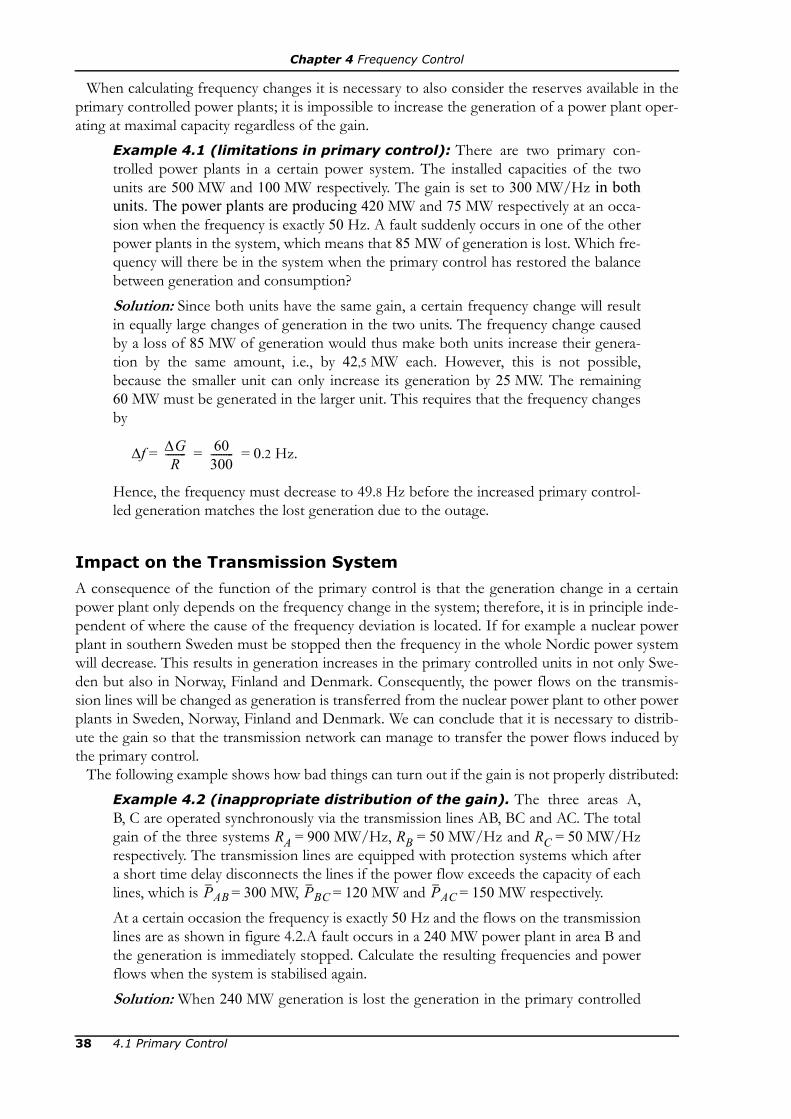
Chapter 4 Frequency Control
When calculating frequency changes it is necessary to also consider the reserves available in theprimary controlled power plants; it is impossible to increase the generation of a power plant oper-ating at maximal capacity regardless of the gain.
Example 4.1 (limitations in primary control): There are two primary con-trolled power plants in a certain power system. The installed capacities of the twounits are 500 MW and 100 MW respectively. The gain is set to 300 MW/Hz in bothunits. The power plants are producing 420 MW and 75 MW respectively at an occa-sion when the frequency is exactly 50 Hz. A fault suddenly occurs in one of the otherpower plants in the system, which means that 85 MW of generation is lost. Which fre-quency will there be in the system when the primary control has restored the balancebetween generation and consumption?Solution: Since both units have the same gain, a certain frequency change will resultin equally large changes of generation in the two units. The frequency change causedby a loss of 85 MW of generation would thus make both units increase their genera-tion by the same amount, i.e., by 42,5 MW each. However, this is not possible,because the smaller unit can only increase its generation by 25 MW. The remaining60 MW must be generated in the larger unit. This requires that the frequency changesby
Δf = = 0.2 Hz.
Hence, the frequency must decrease to 49.8 Hz before the increased primary control-led generation matches the lost generation due to the outage.
Impact on the Transmission System
A consequence of the function of the primary control is that the generation change in a certainpower plant only depends on the frequency change in the system; therefore, it is in principle inde-pendent of where the cause of the frequency deviation is located. If for example a nuclear powerplant in southern Sweden must be stopped then the frequency in the whole Nordic power systemwill decrease. This results in generation increases in the primary controlled units in not only Swe-den but also in Norway, Finland and Denmark. Consequently, the power flows on the transmis-sion lines will be changed as generation is transferred from the nuclear power plant to other powerplants in Sweden, Norway, Finland and Denmark. We can conclude that it is necessary to distrib-ute the gain so that the transmission network can manage to transfer the power flows induced bythe primary control.
The following example shows how bad things can turn out if the gain is not properly distributed:Example 4.2 (inappropriate distribution of the gain). The three areas A,B, C are operated synchronously via the transmission lines AB, BC and AC. The totalgain of the three systems RA = 900 MW/Hz, RB = 50 MW/Hz and RC = 50 MW/Hzrespectively. The transmission lines are equipped with protection systems which aftera short time delay disconnects the lines if the power flow exceeds the capacity of eachlines, which is = 300 MW, = 120 MW and = 150 MW respectively.At a certain occasion the frequency is exactly 50 Hz and the flows on the transmissionlines are as shown in figure 4.2.A fault occurs in a 240 MW power plant in area B andthe generation is immediately stopped. Calculate the resulting frequencies and powerflows when the system is stabilised again. Solution: When 240 MW generation is lost the generation in the primary controlled
ΔGR
-------- 60300---------=
PAB PBC PAC
38 4.1 Primary Control

Chapter 4 Frequency Control
power plants must increase by that amount. The increase is distributed between theareas according to their share of the total gain, RABC, which equals 1 000 MW/Hz:
ΔGA = = 216 MW,
ΔGB = = 12 MW,
ΔGC = = 12 MW.
Since the load in area A remains unchanged the whole generation increase must beexported. There is however only 150 MW free capacity on the connections AB andAC. One of the lines and then the other will be overloaded and disconnected regard-less of how the generation increase in area A is divided between the two lines. Thus,there will be two separate systems: A and B + C respectively.In system A the load and the generation not involved in the primary control is thesame as before the fault in area B. The earlier export of 300 MW has however beenlost, which implies that the primary controlled generation must decrease correspond-ingly. Thus, we will have a frequency increase ΔfA = 300/900 Hz = 0.33 Hz, whichyields fA = 50.33 Hz.In the system B + C there is a deficit of 240 MW due to the failure. Moreover, theimport from area A has been lost, which gives us a total deficit of 540 MW. As bothareas have equally large gain, the generation will increase by 270 MW in both areas. Inarea C, we have an generation increase of 270 MW and a reduced import of 100 MW.There are no changes in load and the generation in those power plants which are notparticipating in the primary control; hence, the export to area B must be increased by170 MW. Thus, that transmission line will also be overloaded.Compared to the situation before the failure, area C has lost an import of 100 MWand an export of 40 MW. This leaves us with a deficit of 60 MW, which gives us thefrequency decrease ΔfC = 60/50 Hz = 1.2 Hz. The frequency in area C must then befC = 48.8 Hz.Area B is now left to its own gain. In total, the area has lost 240 MW generation and240 MW import from areas A and C. The frequency change required to compensatefor the lost generation is ΔfB = 480/50 Hz = 9.6 Hz! Such a large frequency decrease ishowever not acceptable. Probably the system operator will order rotating load curtail-
A
C
200 MWB
40 MW100 MW
Figure 4.2 Transmission before the gener-ation is reduced in area B.
RARABC------------- 240 MW⋅
RBRABC------------- 240 MW⋅
RCRABC------------- 240 MW⋅
4.1 Primary Control 39
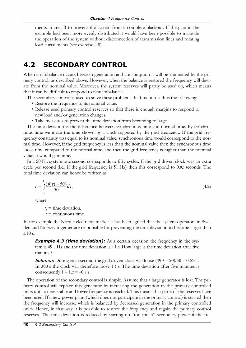
Chapter 4 Frequency Control
ments in area B to prevent the system from a complete blackout. If the gain in theexample had been more evenly distributed it would have been possible to maintainthe operation of the system without disconnection of transmission lines and rotatingload curtailments (see exercise 4.8).
4.2 SECONDARY CONTROLWhen an imbalance occurs between generation and consumption it will be eliminated by the pri-mary control, as described above. However, when the balance is restored the frequency will devi-ate from the nominal value. Moreover, the system reserves will partly be used up, which meansthat it can be difficult to respond to new imbalances.
The secondary control is used to solve these problems. Its function is thus the following:• Restore the frequency to its nominal value.• Release used primary control reserves so that there is enough margins to respond to
new load and/or generation changes.• Take measures to prevent the time deviation from becoming to large.
The time deviation is the difference between synchronous time and normal time. By synchro-nous time we mean the time shown by a clock triggered by the grid frequency. If the grid fre-quency constantly was equal to its nominal value, synchronous time would correspond to the nor-mal time. However, if the grid frequency is less than the nominal value then the synchronous timeloose time compared to the normal time, and then the grid frequency is higher than the nominalvalue, it would gain time.
In a 50 Hz system one second corresponds to fifty cycles. If the grid driven clock sees an extracycle per second (i.e., if the grid frequency is 51 Hz) then this correspond to 0.02 seconds. Thetotal time deviation can hence be written as
ti = (4.2)
where
ti = time deviation,t = continuous time.
In for example the Nordic electricity market it has been agreed that the system operators in Swe-den and Norway together are responsible for preventing the time deviation to become larger than±10 s.
Example 4.3 (time deviation): At a certain occasion the frequency in the sys-tem is 49.8 Hz and the time deviation is +1 s. How large is the time deviation after fiveminutes?Solution: During each second the grid driven clock will loose (49.8 – 50)/50 = 0.004 s.In 300 s the clock will therefore loose 1.2 s. The time deviation after five minutes isconsequently 1 – 1.2 = –0.2 s.
The operation of the secondary control is simple. Assume that a large generator is lost. The pri-mary control will replace this generator by increasing the generation in the primary controlledunits until a new, stable and lower frequency is reached. This means that parts of the reserves havebeen used. If a new power plant (which does not participate in the primary control) is started thenthe frequency will increase, which is balanced by decreased generation in the primary controlledunits. Hence, in that way it is possible to restore the frequency and regain the primary controlreserves. The time deviation is reduced by starting up “too much” secondary power if the fre-
f τ( ) 50–( )50
-------------------------- τ,d0
t
∫
40 4.2 Secondary Control

Chapter 4 Frequency Control
quency has been too low for too long time.Secondary control is a necessary function in all power systems, but it can be implemented in sev-
eral ways. In many power systems the so-called AGC (Automatic Generation Control) is used,which means that the control systems in the power plants in addition to the gain also have an inte-grating part, which eliminates the frequency deviation. AGC is not used in the Nordic synchro-nous grid; instead, all secondary control is managed manually form the control rooms of the sys-tem operators.
It should be noted that if generation is lost in a certain part of the system then it might be neces-sary to start up new generation in the same part of the system in order to prevent the transmissionfrom changing too much.
4.3 COST OF FREQUENCY CONTROLThe frequency control is, as said above, necessary if the power system should be able to functionat all; hence, it can be seen as an example of a technical function which is far more important thaneconomy (cf. section 1.1); the costs caused by a total collapse of the power system is by far largerthan the costs of maintaining the frequency. Still, it can be interesting to have an idea of what iscausing the costs of frequency control.
All power plants have certain operation points where the efficiency is as high as possible. Whenperforming short-term planning of power plants it is of course desirable to use these best effi-ciency points as much as possible. The primary controlled units can however not be planned tooperate at maximum efficiency, as the generation is partly determined by the gain and the systemfrequency. The primary control therefore means that some primary controlled units will be oper-ated at a lower efficiency than the maximal. In most cases the decrease in efficiency is small andthe costs are consequently also rather small.
Another cost for the primary control is that it costs to keep margins in the primary controlledunits. Sometimes it might occur that a more expensive power plant, which is not part of the pri-mary control, is used even though there is unused capacity in a less expensive primary controlledunit. The unused capacity of the primary controlled unit can however not be utilised, since thepower plant then would be unable to increase its generation if the frequency decreases. It is alsopossible that situations occur when a more expensive primary controlled unit is used, even thoughthere is unused capacity in a less expensive power plant which is not participating in the primarycontrol. In this case the primary controlled unit is operated at part capacity in order to be capableof reducing its generation if the frequency should be increased.
The secondary control includes rescheduling the operation of hydro power plants and—in thosesystem where AGC is used—thermal power plants so that better efficiency points can be used, i.e.,a cost decrease. Extra costs can however occur during short time periods when the primary con-trol reserve is restored, for example if an expensive, but fast-started, power plant (for instance agas turbine) is started while waiting for less expensive reserves to be ready for operation.
EXERCISES4.1 A power plant generates 100 MW when the frequency is exactly 50 Hz. When the fre-
quency decreases to 49.95 Hz the power plant increases its generation to 110 MW.What is the gain of this power plant?
4.2 The frequency in a power system is exactly 50 Hz. The total gain in the system is2 000 MW/Hz. Calculate the new frequency when the primary control has restoredbalance after the following events:
4.3 Cost of Frequency Control 41

Chapter 4 Frequency Control
a) The load increases by 100 MW.b) The load decreases by 80 MW.c) A power plant, which is not participating in the primary control, increases its gen-eration by 80 MW.d) A power plant with the gain 200 MW/Hz, which is currently generating 400 MW,is stopped due to a serious fault.
4.3 The total gain in a certain power system is 5 000 MW/Hz. The largest power plant inthe system is a nuclear power plant of 800 MW; this power plant does not participatein the primary control. The second largest power plant is a hydro power plant of650 MW, which has the gain 50 MW/Hz. In which of the following cases will it bepossible to maintain a frequency within the interval 49.9 to 50.1 Hz?a) Generation and consumption are in balance, and the frequency is 50.05 Hz whenthe nuclear power plant — which is operated at maximal generation — must bestopped immediately.b) Generation and consumption are in balance, and the frequency is 49.98 Hz whenthe hydro power plant must be disconnected due to a short-cut in a transformer. Thehydro power plant was generating 400 MW before the error.c) Generation and consumption are in balance, and the frequency is 49.99 Hz. Duringthe half-time pause of a football game, 200 000 TV viewers start making coffee, whichcauses a load increase of 250 MW within just a few minutes.d) The generation exceeds the consumption by 150 MW, and the frequency is49.93 Hz. A stroke of lightning causes a major black-out in a city, which results in aload decrease of 650 MW.e) Generation and consumption are in balance and the frequency is exactly 50 Hz.The time deviation is –16 seconds and it is desired to reduce the deviation to –10 sec-onds within 10 minutes. No other generation or load changes occur during these 10minutes.
4.4 The hydro power plant Fors has the installed capacity 100 MW. It is not possible togenerate less than 40 MW in the power plant, because then there would be a risk ofdamaging the turbines. The gain of the power plant is set to 200 MW/Hz and thegeneration is 70 MW when the frequency is exactly 50 Hz.a) How much is Fors generating when the system frequency is 49.82 Hz?b) How much is Fors generating when the system frequency is 49.94 Hz?c) How much is Fors generating when the system frequency is 50.06 Hz?d) How much is Fors generating when the system frequency is 50.18 Hz?
4.5 The island Ön has two power plants participating in the primary control. The gain ineach power plant is 50 MW/Hz. One of the power plants has an installed capacity of50 MW and generates 44 MW at 8:00 AM. The other power plants has an installedcapacity of 100 MW and generates 62 MW at 8:00 AM.
Ön is connected to Land via an AC transmission line. This line has a maximal trans-mission capacity of 400 MW and is equipped with a protection system which after ashort time delay disconnects the line if the maximal capacity is exceeded. At 8:00 AMthe transmission on the line is 390 MW from Land to Ön.
The power plants located in Land which are participating in the primary control hasa total gain of 4 950 MW/Hz available in the frequency range 50±0.4 Hz.
42 Exercises

Chapter 4 Frequency Control
At 8:00 AM the frequency is 49.98 Hz. Just after that a nuclear power plant isstopped in Land. The nuclear power plant has an installed capacity of 1 200 MW andwas generating 1 006 MW when the failure occurred. a) How much does the electricity generation in Ön increase due to the failure?b) Will the transmission line to Land be able to transfer the generation increase with-out being disconnected?c) Which frequency will be obtained in Land and Ön? Answer with three decimals!
4.6 Assume that a power system is supplied by a thermal power plant with the maximumcapacity 220 MW and three hydro power plants with the capacities 200 MW, 400 MWand 600 MW respectively. At a certain occasion the frequency of the system is exactly50 Hz, the thermal power plant is generating 190 MW and the hydro power plants areoperating at 80% of their installed capacity. The two smaller hydro power plants havea gain of 250 MW/Hz and the largest hydro power plant has the gain 500 MW/Hz.At this occasion the thermal power plant is suddenly stopped. Calculate the systemfrequency and the generation in the hydro power plants when the balance is restored.
4.7 A power system is divided in two areas, A and B. The maximal transmission capacitybetween the two areas is 500 MW. The connections between A and B are equippedwith protection systems which after short time delay disconnects overloaded trans-mission lines. In average, area A exports 200 MW to area B. The dimensioning fault(i.e., the largest production loss which can be caused by a failure in a power plant) is800 MW in area A and 400 MW in area B. The dimensioning fault does not affectpower plants participating in the primary control.a) Assume that it has been decided that the frequency may not drop more than0.2 Hz if a dimensioning fault occurs in either of the areas. How large must the totalgain be then?b) Moreover, assume that it has been decided that the system should be able to man-age a dimensioning fault in either of the areas, which occurs when the power flowbetween the areas correspond to the average, without any transmission lines becom-ing overloaded. How must the total gain be distributed between area A and B?
4.8 Consider the same system as in example 4.2, but assume that the gain is 300 MW/Hzin each area. Check that the system can manage the transmission changes induced bythe primary control and calculate the resulting system frequency.
4.9 Consider the same system as in example 4.2, but assume that the gain in the three sys-tems are RA = 650 MW/Hz, RB = 500 MW/Hz and RC = 450 MW/Hz respectively.At a certain occasion the frequency is exactly 50 Hz and the power flows of the trans-mission lines are as shown in figure 4.3. A short circuit, caused by a stroke of light-ning, causes the protection system to disconnect line AC. Calculate the resulting fre-quencies and the transmission on the tie lines when the system is stabilised again.
4.10 Table 4.2 shows how the total gain is divided among the countries in the synchronousNordel system at a certain occasion. The table also shows the transmission betweenthe countries. At this occasion the frequency is exactly 50 Hz and the time deviation is+1 s. At this occasion a 200 MW coal condensing unit is stopped in Sjælland. Fiveminutes later the load in Norway increases by 100 MW and five minutes after that a300 MW thermal power plant is started in Finland. Calculate the following quantities10 minutes after the start of the Finnish power plant: the frequency, the time devia-tion and the transmission between the countries.
All necessary data are not given for this problem, so one assumption has to be
Exercises 43
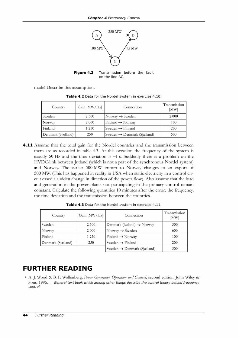
Chapter 4 Frequency Control
made! Describe this assumption.
4.11 Assume that the total gain for the Nordel countries and the transmission betweenthem are as recorded in table 4.3. At this occasion the frequency of the system isexactly 50 Hz and the time deviation is –1 s. Suddenly there is a problem on theHVDC-link between Jutland (which is not a part of the synchronous Nordel system)and Norway. The earlier 500 MW import to Norway changes to an export of500 MW. (This has happened in reality in USA when static electricity in a control cir-cuit cased a sudden change in direction of the power flow). Also assume that the loadand generation in the power plants not participating in the primary control remainconstant. Calculate the following quantities 10 minutes after the error: the frequency,the time deviation and the transmission between the countries.
FURTHER READING• A. J. Wood & B. F. Wollenberg, Power Generation Operation and Control, second edition, John Wiley &
Sons, 1996. — General text book which among other things describe the control theory behind frequencycontrol.
Table 4.2 Data for the Nordel system in exercise 4.10.
Country Gain [MW/Hz] Connection Transmission [MW]
Sweden 2 500 Norway → Sweden 2 000Norway 2 000 Finland → Norway 100Finland 1 250 Sweden → Finland 200Denmark (Sjælland) 250 Sweden → Denmark (Sjælland) 500
Table 4.3 Data for the Nordel system in exercise 4.11.
Country Gain [MW/Hz] Connection Transmission [MW]
Sweden 2 500 Denmark (Jutland) → Norway 500Norway 2 000 Norway → Sweden 600Finland 1 250 Finland → Norway 100Denmark (Sjælland) 250 Sweden → Finland 200
Sweden → Denmark (Sjælland) 500
A
C
250 MWB
75 MW100 MW
Figure 4.3 Transmission before the faulton the line AC.
44 Further Reading

Chapter 5
SHORT-TERM PLANNING
There is a large variety of models and calculations methods that can be used for operation plan-ning of power plants in a system. Although the various models have common characteristics, it isalways necessary at least to some extent to adjust a planning problem to the circumstances at hand.In this chapter we will present a selection of basic models for short-term planning of hydro powerplants and thermal power plants respectively.
The models described in this chapter are linear, and readers who are not familiar with linear pro-gramming are advised to study appendix A in order to better profit from the chapter.
5.1 OBJECTIVE AND CONDITIONSThe objective of a short-term planning is to determine detailed plans how to act for the closest fu-ture. Normally a short-term plan would comprise a time span between a day and a week, which issubdivided into a number of periods. The length of the periods may vary, but the natural choice isto let each period correspond to a trading period in the electricity market—in this description wewill assume that each period corresponds to an hour. Thus, the result of a short-term plan is aplan, which for example states how much each power plant should generate during each hour ofthe planning period. It is also possible to decide how much should be purchased or sold to otherplayers (in particular the power pool).
The Difference Between Short-term Planning and Season Planning
It should be noted that when we in this compendium refer to short-term planning, we mean aproblem where all important factors influencing the operation schedule are known or that there is a reliable fore-cast. In reality this condition will be hard to fulfil. If we for example consider a player who intendto trade at the power exchange Nord Pool, then this player must submit bids of a particular 24-hour period no later than at noon the day before. Then all submitted bids are compiled and it isnotified which bid were accepted and which electricity prices will apply during the 24 hours.Hence, the player must decide how to act before the prices are set and the prices can then be af-fected by the decision made by the player.
When planning the operation it is possible to account for several plausible chains of events; suchplanning problems are in this compendium referred to as season planning problems, as they usu-ally include a longer time perspective than the short-term planning problem. Season planningproblems are much larger than short-term planning problems, and are more difficult to manage
5.1 Objective and Conditions 45
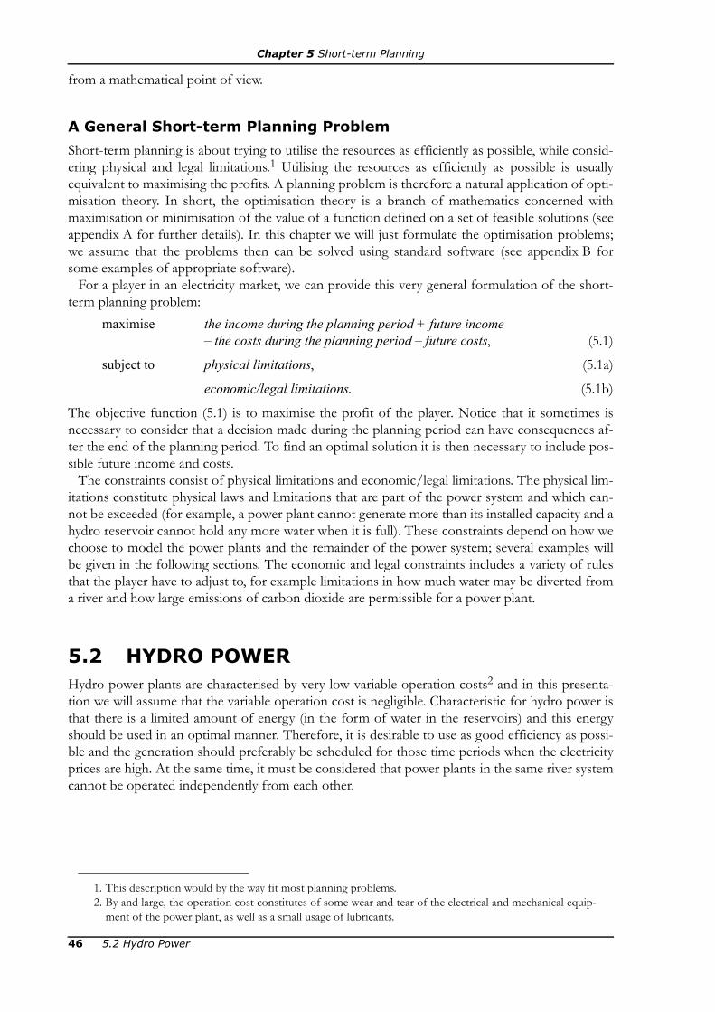
Chapter 5 Short-term Planning
from a mathematical point of view.
A General Short-term Planning Problem
Short-term planning is about trying to utilise the resources as efficiently as possible, while consid-ering physical and legal limitations.1 Utilising the resources as efficiently as possible is usuallyequivalent to maximising the profits. A planning problem is therefore a natural application of opti-misation theory. In short, the optimisation theory is a branch of mathematics concerned withmaximisation or minimisation of the value of a function defined on a set of feasible solutions (seeappendix A for further details). In this chapter we will just formulate the optimisation problems;we assume that the problems then can be solved using standard software (see appendix B forsome examples of appropriate software).
For a player in an electricity market, we can provide this very general formulation of the short-term planning problem:
maximise the income during the planning period + future income – the costs during the planning period – future costs, (5.1)
subject to physical limitations, (5.1a)
economic/legal limitations. (5.1b)
The objective function (5.1) is to maximise the profit of the player. Notice that it sometimes isnecessary to consider that a decision made during the planning period can have consequences af-ter the end of the planning period. To find an optimal solution it is then necessary to include pos-sible future income and costs.
The constraints consist of physical limitations and economic/legal limitations. The physical lim-itations constitute physical laws and limitations that are part of the power system and which can-not be exceeded (for example, a power plant cannot generate more than its installed capacity and ahydro reservoir cannot hold any more water when it is full). These constraints depend on how wechoose to model the power plants and the remainder of the power system; several examples willbe given in the following sections. The economic and legal constraints includes a variety of rulesthat the player have to adjust to, for example limitations in how much water may be diverted froma river and how large emissions of carbon dioxide are permissible for a power plant.
5.2 HYDRO POWERHydro power plants are characterised by very low variable operation costs2 and in this presenta-tion we will assume that the variable operation cost is negligible. Characteristic for hydro power isthat there is a limited amount of energy (in the form of water in the reservoirs) and this energyshould be used in an optimal manner. Therefore, it is desirable to use as good efficiency as possi-ble and the generation should preferably be scheduled for those time periods when the electricityprices are high. At the same time, it must be considered that power plants in the same river systemcannot be operated independently from each other.
1. This description would by the way fit most planning problems.2. By and large, the operation cost constitutes of some wear and tear of the electrical and mechanical equip-
ment of the power plant, as well as a small usage of lubricants.
46 5.2 Hydro Power

Chapter 5 Short-term Planning
5.2.1 General Description of Hydro Power PlantsA hydro power plant generates electric power by utilising the difference in potential energy be-tween an upper and a lower water level. The potential energy is converted to kinetic energy whenthe water is discharged from the upper to the lower water level via a turbine. The turbine in itsturn is driving a generator, where the kinetic energy is transformed to electric energy.
The most important parts of a hydro power plant are shown in figure 5.1. The water is often col-lected in one or more hydro reservoirs, but there are also so-called run-of-the-river hydro powerplants which do not have any possibility to store water. Through the intake the water is led via anheadrace tunnel (or a headrace channel) and the penstock to the turbine itself. The exact layoutvaries from plant to plant and depends on several factors, as for example the bedrock, the headand the distance between reservoir and turbine. Figure 5.1a shows the typical layout of a hydropower plant with low head, where the water is led directly from the intake through a very shortpenstock to the turbine. After passing the turbine, the water is released directly out into the naturalriverbed, which may have been dredged in order to increase the head. It is also possible to spillwater past the power station, by opening gates in the dam.
In figure 5.1b a power plant with higher head is shown. In this case the water is led via a head-race tunnel through the rock before it reaches the penstock. Also the powerhouse and the tailracetunnel are excavated in the rock. The natural riverbed is used if there is a need to spill water pastthe power plant; hence, it is normally drained or has a very reduced water flow.
Discharge, spillage and reservoir contents are all measured in hour equivalents (HE), which cor-responds to the water flow 1 m3/s during 1 hour. Observe that the unit HE sometimes is inter-preted as a volume and sometimes as water flow! It should however always be clear from the con-text what is meant.
5.2.2 Discharge and EfficiencyThe efficiency of a hydro power plant is depending on the head (i.e., the height difference betweenthe water level at the intake and the water level at the end of the tailrace) and the discharge throughthe turbine. The relation between power generation, discharge and head is a non-linear function,which somehow must be approximated by a linear or piecewise linear function in order to be in-cluded in an LP model. The impact of the head is rather small and we will therefore neglect thisfactor. The problem is then to find a linear approximation of the power generation as a functionof the discharge, H(Q).
When calculating the power generation in a hydro power plant it is important to understand thedifference between the following three notions:
Definition 5.1. The production equivalent is the quota between the energy genera-tion and the discharge through the turbines. The production equivalent is different fordifferent discharges. It is denoted by γ and measured in MWh/HE. Given the genera-tion and the discharge, the production equivalent is calculated by
γ(Q) =
Definition 5.2. The marginal production equivalent is a measure of how much thepower generation will increase for a small change of the discharge, i.e., dH(Q)/dQ. Themarginal production equivalent is denoted by μ and is also measured in MWh/HE. Definition 5.3. The relative efficiency normally refers to the production equivalentfor some discharge compared to the maximal production equivalent of the powerplant. The relative efficiency is denoted η and measured in per cent. Given the pro-
H Q( )Q
------------- .
5.2 Hydro Power 47

Chapter 5 Short-term Planning
a) Hydro power plant with low head.
b) Hydro power plant with high head.
Figure 5.1 Overview of the layout of typical Swedish hydropower plants.
HeadTurbine
Generator
Powerhouse
Sub-station
Dam
Sub-station
Sub-station
Natural riverbed
Dam
Intake
Headrace tunnelPenstock
Tailracetunnel
Powerhouse
Powerhouse
Headrace tunnelTailrace tunnel
Draft tube
Hydro reservoir
Hydro reservoir
Hydro reservoir
Hydro reservoir
Intake
Head
48 5.2 Hydro Power
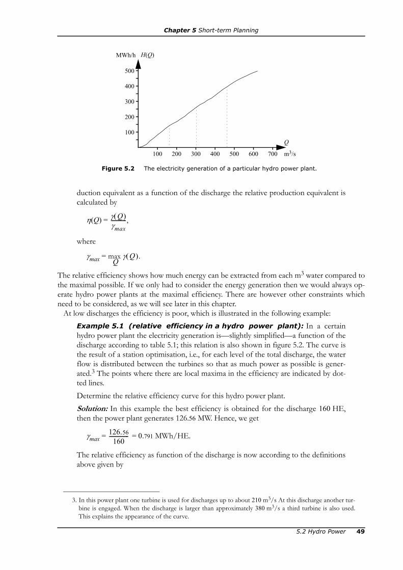
Chapter 5 Short-term Planning
duction equivalent as a function of the discharge the relative production equivalent iscalculated by
η(Q) =
where
γmax =
The relative efficiency shows how much energy can be extracted from each m3 water compared tothe maximal possible. If we only had to consider the energy generation then we would always op-erate hydro power plants at the maximal efficiency. There are however other constraints whichneed to be considered, as we will see later in this chapter.
At low discharges the efficiency is poor, which is illustrated in the following example:Example 5.1 (relative efficiency in a hydro power plant): In a certainhydro power plant the electricity generation is—slightly simplified—a function of thedischarge according to table 5.1; this relation is also shown in figure 5.2. The curve isthe result of a station optimisation, i.e., for each level of the total discharge, the waterflow is distributed between the turbines so that as much power as possible is gener-ated.3 The points where there are local maxima in the efficiency are indicated by dot-ted lines.Determine the relative efficiency curve for this hydro power plant.Solution: In this example the best efficiency is obtained for the discharge 160 HE,then the power plant generates 126.56 MW. Hence, we get
γmax = = 0.791 MWh/HE.
The relative efficiency as function of the discharge is now according to the definitionsabove given by
3. In this power plant one turbine is used for discharges up to about 210 m3/s At this discharge another tur-bine is engaged. When the discharge is larger than approximately 380 m3/s a third turbine is also used.This explains the appearance of the curve.
γ Q( )γmax------------ ,
γ Q( )Q
max .
200 m3/s
Q
MWh/h H(Q)
100 300 400 500 600 700
Figure 5.2 The electricity generation of a particular hydro power plant.
300
400
100
200
500
126.56160
---------------
5.2 Hydro Power 49

Chapter 5 Short-term Planning
η(Q) =
which results in the relative efficiency curve shown in figure 5.3. A piecewise linear model of the power generation in a hydro power plant means that the genera-
tion as function of the discharge is divided into one or more segments. The breakpoints betweenthe segments are preferably located to those discharges where there are local maxima in the effi-ciency, because these discharges are then more likely to appear in the solution of the planningproblem.4 In each segment the marginal production equivalent is approximated by a constant, asshown in figure 5.4. This interpretation means that the total discharge through power plant i mustbe divided in one variable per segment:
Qi, t = (5.2)
where
Qi, t = discharge through power plant i during hour t,Qi, j, t = discharge in power plant i, segment j, during hour t,
ni = number of segments in power plant i.
Table 5.1 The electricity generation of a particular hydro power plant.
Q [m3/s] H [MW] Q [m3/s] H [MW] Q [m3/s] H [MW] Q [m3/s] H [MW]
0 0 160 126.5600 320 248.5638 480 367.9099
20 6.3280 180 139.2476 340 261.6786 500 380.4710
40 18.9840 200 150.7646 360 273.9391 520 392.8106
60 37.9680 220 165.1450 380 285.8516 540 404.5016
80 56.5090 240 181.4870 400 302.7948 560 415.9394
100 74.3540 260 198.6676 420 319.9279 580 426.6654
120 91.7876 280 216.3860 440 336.9027 600 436.6320
140 109.7433 300 233.2659 460 352.9442 620 445.3014
4. To understand why it is like this it would be necessary to further study feasible solutions to LP problems,which is beyond the scope of this compendium.
γ Q( )0.791------------ H Q( )
0.791Q---------------- ,=
200 m3/s
Q
% η(Q)
100 300 400 500 600 700
Figure 5.3 Relative efficiency curve of the hydro power plant in example 5.1.
100
98
96
94
92
90
Qi j t, , ,j 1=
ni
∑
50 5.2 Hydro Power

Chapter 5 Short-term Planning
The total power generation in the power plant is calculated by
Hi, t = (5.3)
where
Hi, t = power generation in power plant i during hour t,μi, j = marginal production equivalent for power plant i, segment j.
In appendix A (examples A.12 and A.13) it is shown that integer variables might be required torepresent a piecewise linear function in a correct manner. In this case we have a certain total dis-charge, which is to be divided between the different segments.5 There is however just one divisionwhich is corresponding to the physical interpretation of the model, i.e., the division where firstsegments are fully utilised before any discharge is made from the next segment. To avoid integervariables, the piecewise linear function must be such that it is more profitable to use the first seg-ment than the second, and the second segment must be preferable to the third, etc. This meansthat the marginal production equivalents have to be decreasing in the linear model (as it is moreprofitable to use a segment having a high marginal production equivalent, since more electricenergy is obtained per HE of water), i.e.,
μi, j > μi, k if j < k. (5.4)
Let us now study an example of a model of a hydro power plant:Example 5.2 (linear model of a hydro power plant): Determine a piece-wise linear model of the hydro power plant in example 5.1.Solution: As discussed above it is important that the model is convex, i.e., the morewater that is discharged the lesser is the efficiency. Such a model can be obtained byusing the local best efficiency points as breakpoints for the piecewise linear function.It can be seen in figure 5.2 and figure 5.3 that the efficiency has a local maximum forthe discharges 60 m3/s, 300 m3/s and 460 m3/s respectively. The electricity genera-tion for these discharges are given in table 5.1.The piecewise linear function is shown in figure 5.4. The marginal production equiva-lents correspond to the slope of the linear segments of the piecewise linear curve:
μ1 = (126.5600 – 0)/(160 – 0) ≈ 0.79 MWh/HE,μ2 = (233.2659 – 126.5600)/(300 – 160) ≈ 0.76 MWh/HE,μ3 = (352.9442 – 233.2659)/(460 – 300) ≈ 0.75 MWh/HE,μ4 = (445.3014 – 352.9442)/(620 – 460) ≈ 0.58 MWh/HE.
Hence, the model for this hydro power plant can be formulated mathematically as
H =
0 ≤ Q1 ≤ 160,
0 ≤ Q2 ≤ 140 (= 300 – 160),
0 ≤ Q3 ≤ 160 (= 460 – 300),
5. For example, Q1 = 20 and Q2 = 0 provides the same total discharge according to (5.2) as Q1 = 0 andQ2 = 20.
μi j, Qi j t, , ,j 1=
ni
∑
μjQj,j 1=
4
∑
5.2 Hydro Power 51

Chapter 5 Short-term Planning
0 ≤ Q4 ≤ 160 (= 620 – 460).
In figure 5.4 we can se that the resemblance between the real electricity generation and the linearmodel is quite good (in particular close to the break points of the piecewise linear function). How-ever, it is also possible to see that for low discharges the linear model is significantly overestimat-ing the electricity generation.6 A straightforward method to avoid this problem is to quite simplyforbid certain discharges. The principle is illustrated in the following example:
Example 5.3 (forbidden discharge domain): Suppose that the productionequivalent as a function of the discharge in a certain power plant i is as shown infigure 5.5. As can be seen in the figure, the efficiency is relatively low for dischargesbelow 50 m3/s (and consequently so is the production equivalent); therefore, theplant should be scheduled so that either more than 50 HE is discharged or nothing atall. Create a linear model of the power generation as a function of the discharge.
6. If we for example consider the electricity generation at the discharge 20 m3/s then the linear model statesthat the generation is 20μ1 ≈ 15.8 MW, whereas it in reality is about 6.3 MW. Thus, the linear model overes-timates the generation by 150%!
200 m3/s
Q
MWh/h H(Q)
100 300 400 500 600 700
Figure 5.4 Piecewise linear model of the electricity generation of the hydropower plant in examples 5.1 and 5.2. The real electricity gener-ation as a function of the discharge is shown by a dotted line.
μ1
μ2
μ3
μ4
Q4Q3
Q2Q1
300
400
100
200
500
100 m3/s
Q
MWh/HE γ(Q)
50 150 200 250 300 350
0.1
Figure 5.5 Example of modelling the electricity generation in a hydropower plant using a mixed integer linear model.
QKi0.3
0.4
0.2
52 5.2 Hydro Power
Chapter 5 Short-term Planning
Solution: For simplicity we choose to divide the generation as function of the dis-charge in only two segments. The first segment includes only one point, namely theorigin. The other segment includes all discharges between 50 HE and maximal dis-charge (300 HE). We assume that the marginal production equivalent in the secondsegment is a constant, μKi, which for example could be chosen as the average of γ(Q)in the interval between 50 and 300 HE. Now we introduce a binary integer variable which represent the active segment duringa certain hour:
zi, t =
The discharge in the continuous segment is denoted by QKi, t. The total discharge inthe power plant can thus be written as
Qi, t = 50zi, t + QKi, t,
which means that the power generation isHi, t = 50μKizi, t + μKiQKi, t.
The equations above will only provide correct results if we introduce a constraintwhich forces the discharge of the second segment to be equal to zero when zi, t = 0.This is achieved by the following inequality constraint:
QKi, t ≤ zi, t.
Finally, we have to introduce variable limits for QKi, t and zi, t:0 ≤ QKi, t,
zi, t ∈ {0, 1}.
It can be noted that avoiding running the power plant at a poor efficiency level is not the onlyreason to forbid certain domains of the discharge. It can also be possible that certain dischargescauses vibrations in the turbines which may result in expensive repairs. The method described inthe example can be generalised to a model where the accepted levels of discharge are no charge atall, a number of local best efficiency points and a continuous interval up to maximal discharge.
5.2.3 Hydrological Coupling Between Hydro Power Plants
In order to use the available water as efficiently as possible it is necessary to coordinate the opera-tion of hydro power plants located in the same river system. The coordination partly has to try toachieve the best possible efficiency in all power plants and partly has to avoid situations wherespillage is necessary (for example if a power plant is operated at maximal discharge even thoughthe downstream reservoir can not store the water). The modelling of the efficiency was describedin the previous section. To avoid spillage it is necessary to consider the hydrological coupling be-tween the power plants, which means that each power plant has to fulfil the following balanceequation:
new reserovir contents = old reservoir contents + water inflow – water outflow. (5.5)
This is a physical necessity and has to be valid for each hour (or any other specified time period).
0 if the discharge is equal to 0 HE,1 if the discharge is larger than or equal to 50 HE.⎩
⎨⎧
QKi
5.2 Hydro Power 53

Chapter 5 Short-term Planning
Mathematically (5.5) is expressed as
Mi, t = Mi, t – 1 – Qi, t – Si, t + Vi, t, (5.6)
where
Mi, t = contents of reservoir i at the end of hour t [HE],Qi, t = discharge in power plant i during hour t [HE],Si, t = spillage past power plant i during hour t [HE],K i = the set of indices for power plants directly upstream of power plant i,τj, i = the delay time for the water between power plant j and the closest down-
stream power plant i [h],Vi, t = local inflow to reservoir i during hour t [HE].
It must be noted that the delay time τji between two power plants is a relatively complex functionof season,7 the water flow and the reservoir levels. For simplicity we assume that the delay time isconstant, i.e., water discharged or spilled from a certain reservoir will reach the next reservoir aftera given number of minutes. Assume that the delay time between j and i is hj hours and mj minutes,independent of the discharge, etc. The following expression for the discharge can then be used:
(5.7)
i.e., a weighted average of the discharge hj and hj + 1 hours earlier. A similar expression can be for-mulated for the spillage.
Juridical restrictions and physical laws imply that reservoir levels as well as discharges are limited.For the last hour in the planning period it is common that there is an upper and a lower limit forthe reservoir contents, which is obtained from long-term plans. These limitations can be formu-lated as
≤ Qi, t ≤ (5.8)
≤ Mi, t ≤ (5.9)
≤ Mi, T ≤ (5.10)
where
= lower limit for discharge in power plant i during hour t,= upper limit for discharge in power plant i during hour t,= lower limit for the contents of reservoir i,= upper limit for the contents of reservoir i,= lower limit for the contents of reservoir i at the end of hour T, i.e., at the end
of the planning period,= lower limit for the contents of reservoir i at the end of hour T.
Generally the allowed reservoir levels are given in metres above the sea level. These limits canhowever easily be translated into limits for the reservoir contents.
5.2.4 Value of Stored WaterWhen planning the operation of hydro power plants it is necessary to consider that the electricity
7. The delay time is for example affected by whether or not the river is icy.
Qj t τj i,–, Sj t τj i,–,j Ki∈∑+
j Ki∈∑+
Qj t τj i,–,mj60------Qj t hj– 1–,
60 mj–60
-----------------Qj t hj–, ,+=
Qi Qi,
Mi Mi,
Mi T, Mi T, ,
QiQiMiMi
Mi T,
Mi T,
54 5.2 Hydro Power

Chapter 5 Short-term Planning
price can vary. At occasions when the electricity price is low it might very well be preferable togenerate nothing at all and rather save the water of the hydro reservoirs for a later occasion, whenthe electricity price is more favourable. Consequently, it is not sufficient to maximise the incomeduring the planning period, but it is also necessary to consider the future income that can be ob-tained from the stored water at the end of the planning period.
There are two methods to include the value of stored water. The most simple is to decide inadvance how much water that should be stored at the end of the planning period. This presetvalue could for example originate from the company long-term plans. A more advanced method isto determine a function to value the water. The value of the water depends partly on how muchelectric energy can be generated from the water and partly on which electricity prices can beexpected when the power is sold, i.e.,
Bi(Mi) = (5.11)
where
Bi(Mi) = value of the water stored in reservoir i,λe = expected electricity price,
Mi, T = contents of reservoir i after the end of the planning period,γj = expected future production equivalent in power plant j,
M i = the set of indices for all power plants downstream of reservoir i (including power plant i itself).
It should be noted that we have to consider that the water in a certain reservoir eventually willreach the reservoirs downstream and therefore will be used for power generation in these powerplants too!
5.2.5 Some Short-term Hydro Power Planning ProblemsIn the previous sections we have shown how to model the electricity generation in hydro powerplants and the hydrological coupling between power plants in the same river system as well as howto calculate the value of stored water. With that, it is time to give a few examples how these modelscan be applied when formulating short-term planning problems for hydro power plants:
Example 5.4 (planning of sales to a power pool): Assume that you are theowner of the hydro power plants Degerforsen and Edensforsen in River Ångermanäl-ven. (Degerforsen is located upstream of Edensforsen.) Data for the two power plantsare given in table 5.2. The electricity generation in the two power plants are sold to apower exchange, where the electricity price the next six hours is forecasted to 165,168, 194, 202, 187 and 183 SEK/MWh respectively. Assume that water which isstored after the sixth hour can be discharged later and that the electricity which then isgenerated will be sold for 185 SEK/MWh. The inflow during the period is equal tothe mean annual flow and the reservoirs are half-filled at the beginning of the plan-ning period. Assume constant efficiency for the power plants, i.e., constant produc-tion equivalent, and that the installed capacity is reached at maximum discharge.Neglect the head losses and the delay time between the power plants. Suggest a dis-charge plan for the two power plants during the next six hours.Solution: Since the operation cost in a hydro power plant is negligible, the planningproblem can be formulated in words as
maximise income of sold energy + value of stored water,subject to hydrological balance in the hydro power plants.
λeMi T, γj,j Mi∈∑
5.2 Hydro Power 55

Chapter 5 Short-term Planning
Before we formulate this problem as an LP problem, we make sure that we havedefined all variables and parameters involved. We start by defining Degerforsen aspower plant number 1 and Edensforsen as number 2. Then we define the optimisa-tion variables (i.e., the variables controlled by the decisions of the company):The following parameters are given directly in the problem text:
= installed capacity in power plant i =
= maximal discharge8 in power plant i =
λf = expected future electricity price = 185,
λ t = expected electricity price during hour t =
The remaining parameters are obtained through simple calculations. The maximal res-ervoir contents9 must be converted from m3 to HE:
= maximal contents of reservoir i =
The start contents is 50% of the maximal, i.e.,
8. Found under the heading “design flow” in table 5.2.9. Found under the heading “active storage of reservoir” in table 5.2. The heading ”volume contents of the
dam” refers to the volume of the dam construction itself.
Table 5.2 Data for Degerforsen and Edensforsen.
Degerforsen Edensforsen
Year of completion 1966 1956Type of power plant Above ground Below groundGross head [m] 24 28Mean annual flow [m3/s] 163 164Design flow[m3/s] 300 270Number and type of turbines 2 × Kaplan 2 × KaplanInstalled capacity[MW] 62 63Average annual energy production [GWh] 295 320Type of dam Rockfill/earthfill EarthfillHeight of dam[m] 18 19Length of dam crest[m] 2 150 700Volume contents of the dam[m3] 235 000 100 000Active storage of the reservoir [m3] 5 000 000 4 000 000Maximum discharge capacity of spillways[m3/s] 1 365 1 350
Hi62 i 1,=63 i 2,=⎩
⎨⎧
Qi300 i 1,=270 i 2,=⎩
⎨⎧
165168194202187183⎩
⎪⎪⎪⎨⎪⎪⎪⎧ t 1,=
t 2,=t 3,=t 4,=t 5,=t 6.=
Mi5 000 000 3 600⁄ 1 389≈4 000 000 3 600⁄ 1 111≈⎩
⎨⎧ i 1,=
i 2.=
56 5.2 Hydro Power

Chapter 5 Short-term Planning
Mi, 0 = start content of reservoir i = 0.5
The local inflow is assumed to be equal to the mean annual flow at Degerforsen. ForEdensforsen the local inflow is equal to the difference between the mean annual flowin the two power plants:
Vi = local inflow to reservoir i =
Finally, we have to calculate the constant production equivalent according to the datain the assignment:
γi = production equivalent in power plant i =
Then we define the optimisation variables (i.e., the variables which are depending onthe decisions of the company):
Qi, t = discharge in power plant i during hour t, i = 1, 2, t = 1, …, 6,Si, t = spillage from reservoir i during hour t, i = 1, 2, t = 1, …, 6,
Mi, t = contents of reservoir i at the end of hour t, i = 1, 2, t = 1, …, 6.The next step is to formulate the objective function:
maximise + λf ((γ1 + γ2)M1(6) + γ2M2(6)).
The constraints are the hydrological balance for Degerforsen and Edensforsenrespectively:
M1, t – M1, t – 1 + Q1, t + S1, t = V1, t = 1, … 6,
M2, t – M2, t – 1 + Q2, t + S2, t – Q1, t – S1, t = V2, t = 1, … 6.
Finally we have to consider the limits for the optimisation variables:0 ≤ Qi, t ≤ i = 1, 2, t = 1, …, 6,0 ≤ Si, t, i = 1, 2, t = 1, …, 6,0 ≤ Mi, t ≤ i = 1, 2, t = 1, …, 6.
Solving the optimisation problem above yield the discharge plan displayed in table 5.3.
Table 5.3 Discharge plan in example 5.4.
Hour, t 0 1 2 3 4 5 6
M1 [HE] 694.4 857.4 1 020.4 883.4 746.4 609.4 772.4M2 [HE] 555.6 556.6 557.6 588.6 619.6 650.6 651.6Q1 [HE] 0 0 300 300 300 0Q2 [HE] 0 0 270 270 270 0
H1 [MWh] 0 0 62 62 62 0H2 [MWh] 0 0 63 63 63 0
S1 [HE] 0 0 0 0 0 0S2 [HE] 0 0 0 0 0 0
Mi694556⎩
⎨⎧ i 1,=
i 2.=≈
163164 163– 1=⎩
⎨⎧ i 1,=
i 2.=
Hi
Qi----- 0.207 i 1,=
0.233 i 2,=⎩⎨⎧
≈
λt γiQi t,i 1=
2
∑t 1=
6
∑
Qi,
Mi,
5.2 Hydro Power 57
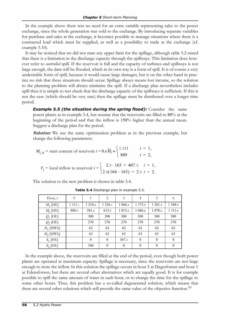
Chapter 5 Short-term Planning
In the example above there was no need for an extra variable representing sales to the powerexchange, since the whole generation was sold to the exchange. By introducing separate variablesfor purchase and sales at the exchange, it becomes possible to manage situations where there is acontracted load which must be supplied, as well as a possibility to trade at the exchange (cf.example 5.10).
It may be noticed that we did not state any upper limit for the spillage, although table 5.2 statedthat there is a limitation in the discharge capacity through the spillways. This limitation does how-ever refer to controlled spill. If the reservoir is full and the capacity of turbines and spillways is notlarge enough, the dam will be flooded, which in its own way is a form of spill. It is of course a veryundesirable form of spill, because it would cause large damages, but it on the other hand in prac-tice no risk that these situations should occur. Spillage always means lost income, so the solutionto the planning problem will always minimise the spill. If a discharge plan nevertheless includesspill then it is simple to test check that the discharge capacity of the spillways is sufficient. If this isnot the case (which should be very rare) then the spillage must be distributed over a longer timeperiod.
Example 5.5 (the situation during the spring flood): Consider the samepower plants as in example 5.4, but assume that the reservoirs are filled to 80% at thebeginning of the period and that the inflow is 150% higher than the annual mean.Suggest a discharge plan for the period.Solution: We use the same optimisation problem as in the previous example, butchange the following parameters:
Mi, 0 = start content of reservoir i = 0.8
Vi = local inflow to reservoir i =
The solution to the new problem is shown in table 5.4.
In the example above, the reservoirs are filled at the end of the period, even though both powerplants are operated at maximum capacity. Spillage is necessary, since the reservoirs are not largeenough to store the inflow. In this solution the spillage occurs in hour 3 at Degerforsen and hour 1at Edensforsen, but there are several other alternatives which are equally good. It is for examplepossible to spill the same amount of water in each hour, or to change the time for the spillage tosome other hours. Thus, this problem has a so-called degenerated solution, which means thatthere are several other solutions which will provide the same value of the objective function.10
Table 5.4 Discharge plan in example 5.5.
Hour, t 0 1 2 3 4 5 6
M1 [HE] 1 111.1 1 218.6 1 326.1 1 066.4 1 173.9 1 281.4 1 388.9M2 [HE] 888.9 581.4 613.9 1 013.6 1 046.6 1 078.6 1 111.6Q1 [HE] 300 300 300 300 300 300Q2 [HE] 270 270 270 270 270 270
H1 [MWh] 62 62 62 62 62 62H2 [MWh] 63 63 63 63 63 63
S1 [HE] 0 0 367.2 0 0 0S2 [HE] 340 0 0 0 0 0
Mi1 111889⎩
⎨⎧ i 1,=
i 2,=≈
2.5 163⋅ 407.5=2.5 164 163–( ) 2.5=⎩
⎨⎧ i 1,=
i 2.=
58 5.2 Hydro Power
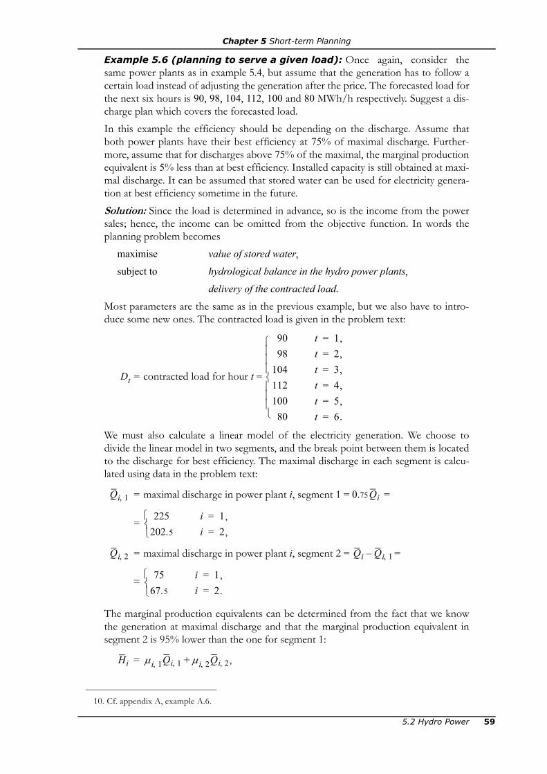
Chapter 5 Short-term Planning
Example 5.6 (planning to serve a given load): Once again, consider thesame power plants as in example 5.4, but assume that the generation has to follow acertain load instead of adjusting the generation after the price. The forecasted load forthe next six hours is 90, 98, 104, 112, 100 and 80 MWh/h respectively. Suggest a dis-charge plan which covers the forecasted load.In this example the efficiency should be depending on the discharge. Assume thatboth power plants have their best efficiency at 75% of maximal discharge. Further-more, assume that for discharges above 75% of the maximal, the marginal productionequivalent is 5% less than at best efficiency. Installed capacity is still obtained at maxi-mal discharge. It can be assumed that stored water can be used for electricity genera-tion at best efficiency sometime in the future.Solution: Since the load is determined in advance, so is the income from the powersales; hence, the income can be omitted from the objective function. In words theplanning problem becomes
maximise value of stored water,subject to hydrological balance in the hydro power plants,
delivery of the contracted load.Most parameters are the same as in the previous example, but we also have to intro-duce some new ones. The contracted load is given in the problem text:
Dt = contracted load for hour t =
We must also calculate a linear model of the electricity generation. We choose todivide the linear model in two segments, and the break point between them is locatedto the discharge for best efficiency. The maximal discharge in each segment is calcu-lated using data in the problem text:
= maximal discharge in power plant i, segment 1 = 0.75 =
=
= maximal discharge in power plant i, segment 2 = =
=
The marginal production equivalents can be determined from the fact that we knowthe generation at maximal discharge and that the marginal production equivalent insegment 2 is 95% lower than the one for segment 1:
10. Cf. appendix A, example A.6.
9098
104112100
80⎩⎪⎪⎪⎨⎪⎪⎪⎧ t 1,=
t 2,=t 3,=t 4,=t 5,=t 6.=
Qi 1, Qi
225202.5⎩
⎨⎧ i 1,=
i 2,=
Qi 2, Qi Qi 1,–
7567.5⎩
⎨⎧ i 1,=
i 2.=
Hi μi 1, Qi 1, μi 2, Qi 2, ,+=
5.2 Hydro Power 59

Chapter 5 Short-term Planning
μi, 2 = 0.95μi, 1.
Solving these systems of equations, we getμi, j = marginal production equivalent of power plant i, segment j ≈
≈
The optimisation variables are also more or less the same as in example 5.4 exceptthat we now need two discharge variables per power plant and hour:Qi, j, t = discharge in power plant i, segment j,during hour t, i = 1, 2, j = 1, 2,
t = 1, …, 6.The objective function in this problem is just the value of stored water:
maximise λf((μ1, 1 + μ2, 1)M1(6) + μ2, 1M2(6)).
The hydrological constraints are almost the same as in example 5.4, but we have somemore variables for the discharge:
M1, t – M1, t – 1 + Q1, 1, t + Q1, 2, t + S1, t = V1, t = 1, … 6,
M2, t – M2, t – 1 + Q2, 1, t + Q2, 2, t + S2, t – Q1, 1, t – Q1, 2, t – S1, t = V2, t = 1, … 6.
The requirement to deliver contracted load is included in the following load balanceconstraints, which in this case states that the total hydro power generation shouldequal the contracted load:
= Dt, t = 1, … 6.
Finally, we have to consider the following limits:0 ≤ Qi, j, t ≤ i = 1, 2, j = 1, 2, t = 1, …, 6,
0.209 i 1 j, 1,= =0.199 i 1 j, 2,= =0.236 i 2 j, 1,= =0.224 i 2 j, 2.= =⎩
⎪⎪⎨⎪⎪⎧
Table 5.5 Discharge plan in example 5.6.
Hour, t 0 1 2 3 4 5 6
M1 [HE] 694.4 656.0 594.0 532.0 460.4 398.4 407.8M2 [HE] 555.6 555.5 565.3 548.4 514.0 515.0 467.1
Q1, 1 [HE] 201.4 225 225 225 225 153.6Q1, 2 [HE] 0 0 0 9.6 0 0Q2, 1 [HE] 202.5 202.5 202.5 202.5 202.5 202.5Q2, 2 [HE] 0 13.6 40.4 67.5 22.6 0Q1 [HE] 201.4 225 225 234.6 225 153.6Q2 [HE] 202.5 216.1 242.9 270 225.1 202.5
H1 [MWh] 42.2 47.1 47.1 49 47.1 32.2H2 [MWh] 47.8 50.9 56.9 63 52.9 47.8
S1 [HE] 0 0 0 0 0 0S2 [HE] 0 0 0 0 0 0
μi j, Qi j t, ,j 1=
2
∑i 1=
2
∑
Qi j, ,
60 5.2 Hydro Power

Chapter 5 Short-term Planning
0 ≤ Si, t, i = 1, 2, t = 1, …, 6,0 ≤ Mi, t ≤ i = 1, 2, t = 1, …, 6.
The solution to this planning problem is shown in table 5.5.
5.3 THERMAL POWERA thermal power plant11 has variable operation cost which is depending on the used fuel and howthe power plant is operated (the efficiency can vary with the loading of the unit). The generationcost is the most important factor when planning the schedule of these power plants, but in wemust also consider that fuel is used when starting a thermal power plant and that the power plantscannot increase or decrease their generation at any rate.
5.3.1 General Description of Thermal Power PlantsA thermal power plant generates electricity by combustion of a fuel. The heat generated at thecombustion is converted to mechanical energy, which is then transformed to electric energy in agenerator.
Thermal power plants can be designed in several ways. In the smallest thermal power plants, thegenerator is powered directly by a regular petrol or diesel engine. This type of thermal power plantis referred to as petrol and diesel generator sets respectively, and may have a rated capacity ofabout 500 W up to about 50 MW. Another type of thermal power plant is gas turbines. Also thesepower plants power the electric generator directly by an engine, but in this case it is of the samekind as the jet engines used in aircraft. Gas turbines for electricity generation typically have a ratedcapacity of about 10 MW to 100 MW. Finally, we have the largest thermal power plants, which arebased on a steam cycle (see figure 5.6). The fuel is combusted in the boiler. Water is pumpedthrough the boiler and heated to steam. The hot steam passes a turbine, which powers the electricgenerator. The steam from the turbine goes back to condenser, where it is cooled down to wateragain and pumped back to the boiler. A nuclear power plant works according to the same basicprinciple, but there are a few variants. In a boiling water reactor the water is heated by the warmthof the nuclear fission and then goes directly to the turbine. In a pressurised water reactor the waterpasses the nuclear reactor under pressure, which causes the water to be heated to several hundreddegrees centigrade without vaporising. The hot water is then passing a steam generator, whichsimply acts as a large heat exchanger; the heat of the water from the reactor transfer is used tovaporise the water in the steam generator. The steam is then passing the turbine, in the same man-ner as for the other steam cycles (see figure 5.6b).
All thermal power plants generate heat as part of the process. A so-called condensing unit onlygenerates electricity. In a combined heat and power plant (CHP) part of the heat is utilised, forexample as district heating. By this means a larger share of the heat content of the fuel is utilised,which results in a higher total efficiency of than for a condensing power plant.
5.3.2 Generation CostThe electricity generation in a thermal power plant depends on the fuel input. If the efficiencywould be constant then a given fuel price would result in a constant operation cost per MWh.However, in practice the efficiency of a thermal power plant is varying depending on the fuel in-put, which thus means that the generation cost becomes a non-linear function of the power out-
11. This footnote has just been added to maintain the footnote numbering in pace with the Swedish edition.
Mi,
5.3 Thermal Power 61

Chapter 5 Short-term Planning
put. To derive a formula for the generation cost of a thermal power plant we start by calculatingthe necessary fuel input for a particular electricity generation:
F(G) = (5.12)
whereF(G) = fuel input as a function of the generation [tonnes/h or m3/h],
G = electricity generation [MWh/h],h = heat contents [MWh/tonnes or MWh/m3] (cf. table 5.6),
η(G) = efficiency at the generation G [%].If the fuel price is φ then we get the following expression for the generation cost:
C(G) = φF(G) = (5.13)
A linear model of the generation cost could be obtained by using a piecewise linear approximationof (5.13)—using similar methods as we used in section 5.2.2 to linearise the electricity generationas function of the discharge in a hydro power plant—but it is more common to approximate(5.13) by a polynomial of degree two:
C(G) = α + βG + γG2. (5.14)
GeneratorTurbine
To the grid
To district heating,
Boiler
Condenser
a) Condensing or CHP plant. A boiling water reactor works in the sameway, but the water is passing a nuclear reactor instead of a boiler.
Figure 5.6 Overview of the layout of larger thermal power plants.
GeneratorTurbine
To the grid
To cooling towerCondenser
Reactor
Steam generator
cooling tower or river
b) Pressurised water reactor.
or river
Gh η G( )⋅-------------------- ,
φ Gh η G( )⋅-------------------- .
62 5.3 Thermal Power

Chapter 5 Short-term Planning
In a LP problem we cannot model the generation cost by a second degree function, but as the co-efficient of the quadratic term, γ, usually is far smaller than the linear coefficient, β, it is in manycases to approximate γ by zeros, which results in a linear function.
5.3.3 Operation ConstraintsWhen planning the operation of a thermal power plant it is necessary to consider that ta change inthe fuel input does not immediately affect the electricity generation. How fast a thermal powerplant can respond to changes depend primarily on its size. Petrol and diesel generator sets are asfast as similar engines in cars; the time scale is thus about seconds. Gas turbines and steam cyclepower plants are slower. In particular, it takes a certain time before these power plants can starttheir generation; gas turbines may take some ten minutes to be started, whereas the largest thermalpower plants may require some hours.
In this section we will give a few examples of how operation constraints can be included in theshort-term planning problem of thermal power plants.
Start-up Costs
Thermal power plants require a certain fuel input to start the process or to prevent that the plantis damaged. It is therefore common that a thermal power plant in addition to the upper limit ofthe electricity generation (which is decided by the installed capacity) also have a lower limit whenthe power plant has been committed. This requirement must be considered in the model of theelectricity generation of a thermal power plant.
Consider a thermal power plant during a certain hour. If the power plant is committed in thishour then the upper limit of the generation is equal to the installed capacity; otherwise, it is equalto zero. This requirement can be expressed as
Gg, t ≤ ug, t· (5.15)
whereGg, t = generation in power plant g during hour t,ug, t = unit commitment in power plant g during hour t (1 if the power plant is
committed, 0 otherwise),= maximal generation when power plant g is committed.
Hence, to determine whether or not the power plant has been committed during a certain periodof the short-term planning problem, we have to introduce a binary integer variable, ug, t. Using this
Table 5.6 Data of some common fuels.
Fuel Heat contents [kWh/kg] Density [kg/m3]
Coal, coke 4.5 - 9.0 450 - 800Diesel oil 11.9 840Petrol 11.9 730Fossil gas 14.4 0.75
Ethanol 7.5 790Wood fuels 5.3a
a. Per kg dry fuel.
310 - 470Uranium 880 000 18 680
Gg,
Gg
5.3 Thermal Power 63

Chapter 5 Short-term Planning
variable we may also represent the lower limit of the electricity generation:
Gg, t ≥ ug, t· (5.16)
where
= minimal generation when power plant g is committed.When the power plant has been committed the lower limit is equal to and when the powerplant is off-line the lower limit is equal to zero. Combined, the two equations (5.15) and (5.16)forces the generation Gg, t to the interval when ug, t equals one (i.e., when the powerplant is committed). When ug, t is equal to zeros, the only possibility to fulfil both constraints is toset Gg, t = 0.
Starting up a thermal power plant results in a certain cost, as some fuel is used to heat the powerplant to operational temperature. In small thermal power plants, this cost is low, but in larger unitsit might be significant. The amount of fuel necessary to heat the boiler depends on its currenttemperature, which in its turn is depending on how long it was since the power plant was takenoff-line. The start-up cost can be written as t
Cstart-up(t) = Ccold-start(1 – e–t/τ) + Cfixed, (5.17)
whereCstart-up(t) = start-up cost after an off-line period of t hours,Ccold-start = start-up cost when the boiler is cooled to room temperature,
τ = thermal time constant of the boiler,Cfixed = fixed start-up cost.
In (5.17) we also have a fixed cost, which for example can include extra staff and maintenancecosts for start-up of the power plant.
Example 5.7 (start-up cost in a thermal power plant): Assume that thecold-start cost of a particular thermal power plant is 1 000 ¤, that the thermal timeconstant of the boiler is 2 hours and that there are no fixed start-up costs. How manyhours after the unit has been taken off-line will it take before the start-up cost is 90%of the cold-start cost? How large is the start-up cost for the intermediate hours?(Assume that the power plant always is started after a number of complete hours.)Solution: We want the time t such that Ccold-start(1 – e–t/τ) ≥ 0.9Ccold-start, i.e.,
t ≥ –2 ln(0.1) = 4.6,The result is therefore that the start-up cost exceeds 900 ¤ after five hours.The start-up cost when the power plant is started after 1, …, 5 hours is given by
Cstart-up(1) = 1 000(1 – e–1/2) ≈ 393 ¤,Cstart-up(2) = 1 000(1 – e–2/2) ≈ 632 ¤,Cstart-up(3) = 1 000(1 – e–3/2) ≈ 777 ¤,Cstart-up(4) = 1 000(1 – e–4/2) ≈ 865 ¤,Cstart-up(5) = 1 000(1 – e–5/2) ≈ 918 ¤.
If the power plant only will be off-line for a short time i might be profitable to not stop the com-bustion in the boiler even though no electricity is generated (so-called banking). In this case, thefuel input is kept just above what is necessary to maintain the operation temperature of the boiler.This fuel input can be assumed to be constant, which makes the start-up cost directly proportionalto the time the power plant has been off-line:
Gg,
Gg,
Gg t,
Gg t, Gg t,,[ ]
64 5.3 Thermal Power

Chapter 5 Short-term Planning
Cstart-up = Cbanking · t (5.18)
Example 5.8 (banking): Consider the same power plant as in example 5.7 andassume that banking costs 250¤/h. How long must the power plant be off-line tomake it more profitable to stop the combustion in the boiler and let it start coolingdown?Solution: We want the time t such that 1 000(1 – e–t/2) = 250t. This equation must besolved numerically; then we find that t ≈ 3.19 h, i.e., if the power plant is to stay off-line at most three hours, banking is preferable, but if it should be off-line four hoursor more then it is better to let the boiler start cooling.
To include the start-up cost in the objective function, we need to introduce more binary varia-bles, which are equal to one the hour when the power plant is started and equal to zero the otherhours. As we seen above, the start-up cost depends on the time the power plant has been off-lineand we therefore need to introduce separate start-up variables for the off-line times we wish toconsider. For the sake of simplicity, let us assume that we only need to differentiate between off-line times of one hour or at least two hours.12 Introduce the following variables:
= start-up of power plant g during hour t after one hour down time (1 if the power plant is started after one hour down time, otherwise 0),
= start-up of power plant g during hour t after at least two hours down time (1 if the power plant is started after at least two hours down time, otherwise 0).
The total start-up cost during the planning period is then expressed as
(5.19)
where= start-up cost when power plant g is started after one hour down time,= start-up cost when power plant g is started at least two hours down time.
As there is a cost associated to non-zero start-up variables, the LP solver will try to set all start-upvariables to equal zero. Therefore, special constraints are necessary to guarantee that the start-upvariables are given the right value whenever the power plant is started:
≥ ug, t – ug, t – 1 – ug, t – 2, (5.20)
≥ ug, t – ug, t – 1 – . (5.21)
Table 5.7 demonstrates that these constraints provide the desired results. (Please note that wemust know the state of the power plants for the two hours before the first hour of the planningperiod.) The right hand side of (5.20) is the lower limit of the start-up variable and this lowerlimit must equal one only if the power plant is committed in hour t and has been off-line duringthe previous two hours. As is a binary variable, the start-up variables must equal one in thesecases. In all other cases the lower limit is zero or negative, and then the start-up variable will equalzero in the optimal solution.
In a similar manner is the right hand side of (5.21) the lower limit for the start-up variable .In this case the lower limit is equal to one only if the power plant is committed in hour t and hasbeen off-line the previous hour. Moreover, the start-up variable must equal zeros, as bothstart-up variables of a power plant cannot be equal to one during the same hour.
12. The reasoning that follows is of course easy to modify to take other possible off-line times into account.
sg t,*
sg t,**
Cg*sg t,* Cg**sg t,**+( ),t T∈∑
g G∈∑
Cg*Cg**
sg t,**
sg t,* sg t,**
sg t,**
sg t,**
sg t,*
sg t,**
5.3 Thermal Power 65

Chapter 5 Short-term Planning
Minimal Up and Down Time
It is not unusual in unit commitment problems to use simpler models of the start-up costs, wherethe start-up costs are assumed to be constant. As a compensation we can introduce a requirementof the down time of a decommitted unit and the up time of a committed unit. Introduce the fol-lowing variables:
= start-up variable for power plant g during hour t (1 if the power plant is started before this hour, otherwise 0),
= stop variable for power plant g during hour t (1 if the power plant is stopped before this hour, otherwise 0).
The total start and stop cost can then be written as
(5.22)
where= start-up cost of power plant g,= stop cost of power plant g.
The requirement of minimal up and down time are formulated as follows:
+ ≤ 1, (5.23)
+ ≤ 1, (5.24)
Table 5.7 Verification of the constraints (5.20) and (5.21).
Hour
–1 0 1 2 3 4
Case I (one hour down time)State, ut 1 1 0 1 1 1Lower limit for start-up after at least twohours off-line, ut – ut – 1 – ut – 2
–2 0 0 –1
Lower limit for start-up after one houroff-line, ut – ut – 1 – –1 1 0 0
Case II (two hours down time)State, ut 1 1 0 0 1 1Lower limit for start-up after at least twohours off-line, ut – ut – 1 – ut – 2
–2 –1 1 0
Lower limit for start-up after one houroff-line, ut – ut – 1 – –1 0 0 0
Case III (three hours down time)State, ut 1 1 0 0 0 1Lower limit for start-up after at least twohours off-line, ut – ut – 1 – ut – 2
–2 –1 0 1
Lower limit for start-up after one houroff-line, ut – ut – 1 – –1 0 0 0
st**
st**
st**
sg t,+
sg t,–
Cg+sg t,
+ Cg–sg t,
–+( ),t T∈∑
g G∈∑
Cg+
Cg–
sg t,+ sg k,
–
k t=
t tg+ 1–+
∑
sg t,– sg k,
+
k t=
t tg– 1–+
∑
66 5.3 Thermal Power

Chapter 5 Short-term Planning
where= minimal up time of power plant g,= minimal down time of power plant g.
If a power plant is started in hour t, i.e., when = 1, the constraint (5.23) forces to becomezero for the next hours; thus, the power plant cannot be taken off-line during this period. Theconstraint (5.24) works in a similar way.
If the requirement of minimal up and down time should have any effect then we must also havea constraint which forces the start-up and stop variables to get the correct values whenever thestate of a unit is changed. This is simply achieved by the following constraint:
ug, t – ug, t – 1 = – . (5.25)
It is easy to verify that this constraint forces and to behave as we desire. If the powerplant is committed then ug, t = 1 and ug, t – 1 = 0, i.e., the left hand side is equal to one. The onlyway for the right hand side to become one is to let = 1; hence, the start-up variable is forcedto become one when the power plant is started. When the power plant is taken off-line the lefthand side equals minus one and the only solution then is to choose = 1. If the state of the unitremains the same then the left hand side is zero and (5.25) can be fulfilled either by setting =
= 1 or by setting = = 0. As start-up and stop of a power plant is associated to a costaccording to (5.22), it will be optimal to choose the latter alternative.
Limited Generation Changes
A large thermal power plant cannot increase or decrease its generation at any rate. To increase thegeneration the boiler must be supplied more thermal energy (to increase the steam flow), whichrequires some time. It is neither possible to reduce the generation at any rate, as the steam is cool-ing the boiler and if the flow is interrupted to abruptly then there is a risk of damaging the boiler.In the planning problem it might therefore be necessary to include ramping constraints, whichlimit how much the generation may change from one hour to another.
Let us start by considering a generation increase. A limitation of the permissible generationincrease from one hour to the next means that the difference in generation between one hour andthe previous one, i.e., Gg, t – Gg, t – 1, must be below a certain maximal generation increase, Unfortunately, this requirement is only valid for those hours when the unit has been committedalso the previous hour. The first hour after the power plant has been started the generationincrease can exceed if the minimal generation, is larger than Assume that themaximal generation during the first hour the power plant is being committed is We may thenexpress the above reasoning as the following constraint:
Gg, t – Gg, t – 1 ≤ + (5.26)
This constraint is verified in table 5.8. In those cases when the power plant is off-line in hour t, i.e.,when ug, t = 0, the maximal generation increase is of no interest, as the power plant cannot in-crease its generation when it is off-line. In the other two cases we see that the maximal generationincrease is equal to if the power plant was committed the previous hour too, and that it be-comes equal to maximal generation capacity the first hour after start-up if the power plant was off-line the previous hour.
A similar constraint is applied for generation decrease:
Gg, t – 1 – Gg, t ≤ + (5.27)
tg+
tg–
sg t,+ sg t,
–
tg+
sg t,+ sg t,
–
sg t,+ sg t,
–
sg t,+
sg t,–
sg t,+
sg t,– sg t,
+ sg t,–
ΔgG+.
ΔgG+ Gg, Δg
G+.Gg
1.
ΔgG+ sg t,
+ Gg1 Δg
G+–( ).
ΔgG+
ΔgG– sg t,
– Gg ΔgG––( ).
5.3 Thermal Power 67

Chapter 5 Short-term Planning
5.3.4 Some Unit Commitment ProblemsIn the previous sections we have shown how to model the generation cost of thermal powerplants, and the operation constraints of larger thermal power plants. With that, it is time to give afew examples how these models can be applied in unit commitment problems:
Example 5.9 (planning of sales to a power pool). Kraftbolaget AB ownsthe thermal power plant Sotinge. The power plant has three blocks, i.e., separate boil-ers and turbines; data for these are given in table 5.9. The electricity generation ofSotinge is sold to the power pool ElKräng. Kraftbolaget AB are now about to submitbids from midnight to midday the following day. A forecast of the electricity prices forthis period is given in table 5.10. Assume that the start-up cost is independent of thedown time and that the stop cost is negligible. According to the plan for the currentday, block I will be committed until midnight, whereas the other two blocks are takenoff-line at 8 pm. Suggest a operation plan for the three blocks during the first twelvehours of the next day.
Solution: In words the problem can be formulated asmaximise income of sold electricity – generation costs – start-up costs
Table 5.9 Data for the fictitious thermal power plant Sotinge.
Sotinge I Sotinge II Sotinge III
Installed capacity [MW] 240 110 170Minimal generation when committed [MW] 80 40 60Generation cost [SEK/MWh] 300 310 320Start-up cost [SEK/start] 25 000 13 000 20 000Minimal up time [h] 3 3 3Minimal down time [h] 3 3 3
Table 5.10 Expected electricity prices at ElKräng.
Hour Price [SEK/MWh] Hour Price [SEK/MWh] Hour Price [SEK/MWh]
1 316 5 309 9 3592 313 6 318 10 3553 306 7 342 11 3484 299 8 353 12 344
Table 5.8 Verification of the constraints (5.26) and (5.27).
State of the previous hour,
ug, t – 1
State of the hour at hand, ug, t
Maximal generation increase, Maximal generation decrease,
0 0
0 1
1 0
1 1
ΔgG+ sg t,
+ Gg1
ΔgG+–( )+ Δg
G– sg t,– Gg Δg
G––( )+
ΔgG+ Δg
G–
Gg1 Δg
G–
ΔgG+ Gg
ΔgG+ Δg
G–
68 5.3 Thermal Power

Chapter 5 Short-term Planning
subject to limitations in generation capacity,minimal up and down times.
Before we start formulating this problem as a MILP problem we make sure that wedefine the variables and parameters that are used in the problem. We start by definingthe blocks as unit 1, 2 and 3 respectively.The following parameters are given in the problem text:
ug, 0 = commitment of unit g at the beginning of the planning period =
λt = expected electrictiy price hour t =
= installed capacity of power plant g =
= minimal generation when power plant g is committed =
βGg = variable generation cost in power plant g =
= start-up cost in power plant g =
Then we state the optimisation variables used in the problem:Gg, t = generation in power plant g, hour t, g = 1, 2, 3, t = 1, …, 12,ug, t = unit commitment of power plant g during hour t, g = 1, 2, 3, t = 1, …, 12,
= start-up variable for power plant g hour t, g = 1, 2, 3, t = 1, …, 12,= stop variable for power plant g hour t, g = 1, 2, 3, t = 1, …, 12.
The objective of the planning is to maximise the income of sold electricity minus thevariable generation costs and the start-up costs, which gives us the following objectivefunction:
maximise
100⎩
⎪⎨⎪⎧ g 1,=
g 2,=g 3,=
316313306299309318⎩
⎪⎪⎪⎨⎪⎪⎪⎧ t 1,=
t 2,=t 3,=t 4,=t 5,=t 6,=
342353359355348344
t 7,=t 8,=t 9,=
t 10,=t 11,=t 12,=
Gg
240110170⎩
⎪⎨⎪⎧ g 1,=
g 2,=g 3,=
Gg
804060⎩
⎪⎨⎪⎧ g 1,=
g 2,=g 3,=
300310320⎩
⎪⎨⎪⎧ g 1,=
g 2,=g 3,=
Cg+
25 00013 00020 000⎩
⎪⎨⎪⎧ g 1,=
g 2,=g 3.=
sg t,+
sg t,–
λt βG–( )Gg t, Cg+sg t,
+–( ).g 1=
3
∑t 1=
12
∑
5.3 Thermal Power 69

Chapter 5 Short-term Planning
The constraints of this problem should limit the generation in each power plant aswell as force the power plants to remain on-line for at least three hours after beingstarted and remain off-line for at least three hours after the being stopped. The gener-ation limitations are managed by the following constraints:
Gg, t – ug, t ≤ 0, g = 1, 2, 3, t = 1, …, 12,
ug, t – Gg, t ≤ 0, g = 1, 2, 3, t = 1, …, 12.
The next constraint sets the relation between unit commitment, start and stop:
ug, t – ug, t – 1 – + = 0, g = 1, 2, 3, t = 1, …, 12.
Then we have the constraints which represents the minimal up and down timesrespectively:
+ + ≤ 1, g = 1, 2, 3, t = 1, …, 10,
+ ≤ 1, g = 1, 2, 3, t = 11,
+ + ≤ 1, g = 1, 2, 3, t = 1, …, 10,
+ ≤ 1, g = 1, 2, 3, t = 11.
Finally we state the variable limits. Notice that the upper and lower limits of Gg, t iscontrolled by the constraints for generation limitations; hence, Gg, t can be consideredas a free variable.
ug, t ∈ {0, 1}, g = 1, 2, 3, t = 1, …, 12,
∈ {0, 1}, g = 1, 2, 3, t = 1, …, 12,
∈ {0, 1}, g = 1, 2, 3, t = 1, …, 12.
Solving the optimisation problem above yield the operation plan displayed intable 5.11.
Gg
Gg
sg t,+ sg t,
–
sg t,+ sg t 1+,
– sg t 2+,–
sg t,+ sg t 1+,
–
sg t,– sg t 1+,
+ sg t 2+,+
sg t,– sg t 1+,
+
sg t,+
sg t,–
Table 5.11 Operation plan in example 5.9.
Hour, t 1 2 3 4 5 6 7 8 9 10 11 12
G1, t [MW] 240 240 240 80 240 240 240 240 240 240 240 240G2, t [MW] 110 110 40 40 40 110 110 110 110 110 110 110G2, t [MW] 0 0 0 0 0 0 170 170 170 170 170 170
u1, t 1 1 1 1 1 1 1 1 1 1 1 1u2, t 1 1 1 1 1 1 1 1 1 1 1 1u3, t 0 0 0 0 0 0 1 1 1 1 1 1
0 0 0 0 0 0 0 0 0 0 0 01 0 0 0 0 0 0 0 0 0 0 00 0 0 0 0 0 1 0 0 0 0 00 0 0 0 0 0 0 0 0 0 0 00 0 0 0 0 0 0 0 0 0 0 00 0 0 0 0 0 0 0 0 0 0 0
s1 t,+
s2 t,+
s3 t,+
s1 t,–
s2 t,–
s3 t,–
70 5.3 Thermal Power

Chapter 5 Short-term Planning
In the example above we see that two of the blocks are committed even when the electricityprice is less than the variable generation cost. The explanation is of course that it is so expensive torestart the units after decommitting them that it is cheaper to generate some electricity at a loss.Therefore, the generation is reduced as much as possible without stopping the unit.
Example 5.10 (planning of bilateral trade and sales to power pool):Consider Sotinge power plant again, but assume that Kraftbolaget AB also has a bilat-eral contract to sell 200 MWh/h to AB Elleverantören.In this example a variable start-up cost should be used instead of minimal up- anddown times. Assume that the start-up costs given in example 5.9 correspond to thecold-start cost and that the thermal time constants are 2.5 hours in block I, 1.5 hoursin block II, and 2 hours in block III. After three hours of down time, the start-up costis assumed to equal the cold-start cost.Solution: The income of the firm power contract does not influence the operation ofthe power plants; therefore, it can be omitted from the objective function. In wordsthe planning problem may then be expressed as
maximise income of sold electricity – generation costs – start-up costssubject to limitations in generation capacity,
start-up constraints,load balance.
Most of the parameters are the same as in example 5.9, but we also need to introducea few new ones. The firm sales and the thermal time constants are given above:
D = firm power sales = 200,
τ = thermal time constants =
In the previous example it was sufficient to know the state of the units the hourbefore the beginning of the planning period. In this case we must know the state forthree hours last three hours when calculating the start-up costs of the power plants.
ug, t = unit commitment of power plant g the hours before the start of the planning
period =
The cold-start cost and the start-up cost after at least three hours down time isassumed to be the same as the cost in table 5.9. The start-up cost for shorter downtimes are calculated according to (5.17):
= start-up cost after at least three hours down time =
= start-up cost after two hours down time =
2.51.52⎩
⎪⎨⎪⎧ g 1,=
g 2,=g 3.=
10⎩
⎨⎧ g 1, t 2 1 0,,–,–= =
g 2 3, t, 2 1 0,,–,–= =
Cg***25 00013 00020 000⎩
⎪⎨⎪⎧ g 1,=
g 2,=g 3.=
Cg**
5.3 Thermal Power 71

Chapter 5 Short-term Planning
=
= start-up cost after one hour down time =
=
The start and stop variables of example 5.9 are not used here, but we will introducethree separate start-up variables for start-up after a given down time. We must alsointroduce variables for the trade at ElKräng. Hence, we get the following optimisationvariables in this problem:
Gg, t = generation in power plant g, hour t, g = 1, 2, 3, t = 1, …, 12,ug, t = unit commitment in power plant g during hour t, g = 1, 2, 3, t = 1, …, 12,
= start-up of power plant g in hour t after at least three hours down time, g = 1, 2, 3, t = 1, …, 12,
= start-up of power plant g in hour t after two hours down time, g = 1, 2, 3, t = 1, …, 12,
= start-up of power plant g in hour t after one hour down time,g = 1, 2, 3, t = 1, …, 12,
pt = purchase from ElKräng hour t, t = 1, …, 12,rt = sales to ElKräng hour t, t = 1, …, 12.
The objective function is now to maximise the income of sold electricity minus thecosts of purchase, generation and start-ups:
maximise
The generation limitations are the same as before:
Gg, t – ug, t ≤ 0, g = 1, 2, 3, t = 1, …, 12,
ug, t – Gg, t ≤ 0, g = 1, 2, 3, t = 1, …, 12.
Then we have the constraints that make sure the start-up variables are given the cor-rect values:
ug, t – ug, t – 1 – ug, t – 2 – ug, t – 3 – ≤ 0, g = 1, 2, 3, t = 1, …, 12,
ug, t – ug, t – 1 – ug, t – 2 – – ≤ 0, g = 1, 2, 3, t = 1, …, 12,
ug, t – ug, t – 1 – – – ≤ 0, g = 1, 2, 3, t = 1, …, 12.
We also need load balance constraints to guarantee that the company’s own genera-tion plus purchase are equal to the firm power contract plus sales to the power pool:
+ pt – rt = Dt, t = 1, …, 12.
Finally we state the variable limits. Notice that the upper and lower limits of Gg, t is
1 e 2 τ/––( )Cg***13 7679 573
12 642⎩⎪⎨⎪⎧ g 1,=
g 2,=g 3.=
≈
Cg*
1 e 1 τ/––( )Cg***8 2426 3267 869⎩
⎪⎨⎪⎧ g 1,=
g 2,=g 3.=
≈
sg t,***
sg t,**
sg t,*
λt rt pt–( ) βGgGg t, Cg***sg t,*** Cg**sg t,** Cg*sg t,* + + +( )g 1=
3
∑–⎝ ⎠⎜ ⎟⎛ ⎞
.t 1=
12
∑
Gg
Gg
sg t,***
sg t,*** sg t,**
sg t,*** sg t,** sg t,*
Gg t,g 1=
3
∑
72 5.3 Thermal Power

Chapter 5 Short-term Planning
controlled by the constraints for generation limitations; hence, Gg, t can be consideredas a free variable.
ug, t ∈ {0, 1}, g = 1, 2, 3, t = 1, …, 12,
∈ {0, 1}, g = 1, 2, 3, t = 1, …, 12,
∈ {0, 1}, g = 1, 2, 3, t = 1, …, 12,
∈ {0, 1}, g = 1, 2, 3, t = 1, …, 12,
0 ≤ pt, t = 1, …, 12,
0 ≤ rt, t = 1, …, 12.
Solving the optimisation problem above yield the operation plan displayed intable 5.12.
5.4 DUAL VARIABLESUsually when solving an LP problem, the solution also includes the value of the so-called dual vari-ables (see appendix A, examples A.8-A.10). One dual variable can be obtained for each constraintand for each variable limit. The dual variables show how much the optimal value would change if asmall change is made to the right hand side of the corresponding constraint13 and for smallchanges of the variable limits. In practice it is not very convenient to use the dual variables in thismanner, as it is hard to know in advance whether or not a change is “large” or “small”—if theproblem is not extremely large and difficult to solve it is generally preferable to simply solve the
13. This requires that the problem is formulated in standard form, i.e., all terms including optimisation varia-bles should be in the left hand side, while the right hand side only includes known parameters.
sg t,***
sg t,**
sg t,*
Table 5.12 Operation plan in example 5.10.
Hour, t 1 2 3 4 5 6 7 8 9 10 11 12
G1, t [MW] 240 240 240 80 240 240 240 240 240 240 240 240G2, t [MW] 110 110 40 40 40 110 110 110 110 110 110 110G2, t [MW] 0 0 0 0 0 0 170 170 170 170 170 170
u1, t 1 1 1 1 1 1 1 1 1 1 1 1u2, t 1 1 1 1 1 1 1 1 1 1 1 1u3, t 0 0 0 0 0 0 1 1 1 1 1 1
0 0 0 0 0 0 0 0 0 0 0 01 0 0 0 0 0 0 0 0 0 0 00 0 0 0 0 0 1 0 0 0 0 00 0 0 0 0 0 0 0 0 0 0 00 0 0 0 0 0 0 0 0 0 0 00 0 0 0 0 0 0 0 0 0 0 00 0 0 0 0 0 0 0 0 0 0 00 0 0 0 0 0 0 0 0 0 0 00 0 0 0 0 0 0 0 0 0 0 0
pt 0 0 0 80 0 0 0 0 0 0 0 0rt 150 150 80 0 800 150 320 320 320 320 320 320
s1 t,***s2 t,***s3 t,***s1 t,**s2 t,**s3 t,**s1 t,*s2 t,*s3 t,*
5.4 Dual Variables 73

Chapter 5 Short-term Planning
new problem directly.The interesting about dual variables is rather that they do not just have a mathematical meaning,
but they also have practical interpretation in reality. The objective function of a short-term plan-ning problem corresponds to the profit or costs during the planning period; hence, the dual varia-bles state how much the profit or costs will change for small changes of the prerequisites of theplanning problem. We may therefore consider the dual variables as a sort of derivatives of benefitand cost functions. This means that the dual variables can be interpreted as various prices,14 asdemonstrated in the following examples:
Example 5.11 (dual variables of hydrological balance constraints).Which unit has the dual variables of a hydrological balance constraint? Are these dualvariables going to be larger than zero, equal to zero or lesser than zero? What practicalinterpretation can be given these dual variables? Assume that the short-term planningproblem is formulated as maximisation of the profits.Solution: The unit of the objective function is currency (¤) and the unit of the hydro-logical balance constraint is HE. The dual variables thus states how the profits willchange for a change in the right hand side of the problem when stated in standardform, which means that only the local inflow will be found in the right hand side. Theunit must therefore be ¤/HE. During normal conditions an increased inflow will result in increased income (eitherby generating more electricity or by having more water stored in the reservoirs at theend of the planning period), which means that the dual variables must be larger thanzero. However, this is not valid if the inflow is so large that water has to be spilled; inthis case the income is not affected by increased inflow and the dual variables get thevalue zero.In practice these dual variables correspond to a price which might be associated to thewater in a certain reservoir. This price is referred to as water value.Example 5.12 (dual variables of load balance constraints). Which unithas the dual variables of a load balance constraint? Are these dual variables going tobe larger than zero, equal to zero or lesser than zero? What practical interpretation canbe given these dual variables? Assume that the short-term planning problem is formu-lated as maximisation of the profits.Solution: The unit of the objective function is currency (¤) and the unit of the hydro-logical balance constraint is MWh. The dual variables thus states how the profits willchange for a change in the right hand side of the problem when stated in standardform, which means that only the load will be found in the right hand side. The unitmust therefore be ¤/MWh. If the load increases then the value of the objective function decreases. Admittedly,the income of sold electricity increases during the planning period, but if the load isgiven in advance then this income are also given in advance and will not be accountedfor in the objective function. On the other hand is the generation cost increasing (inthermal power plants) or there will be a less amount of water stored at the end of theperiod. The dual variable is therefore negative or—in some rare cases—equal to zero.In practice these dual variables correspond to the marginal production cost of theplayer performing the planning. If there is perfect competition in the market then thisvalue also corresponds to the electricity price.
14. Therefore, economic literature frequently uses the notion “shadow prices” instead of dual variables.
74 5.4 Dual Variables

Chapter 5 Short-term Planning
The dual variables are also useful for checking that a correct optimal solution has been found forthe planning problem. The dual variables of interest are in general less than the primal variables ofinterest; hence, it is less work to study the dual variables. Moreover, it is easier to check that theprices in the system are reasonable than to study the relation of the primal variables in detail. Thisis illustrated in the following examples:
Example 5.13 (checking the operation plan). Consider the planning prob-lem in example 5.4, but assume that the electricity prices of the six hours are fore-casted to 213, 225, 229, 227, 230 and 232 SEK/MWh respectively and that the futureelectricity generation is assumed to be sold for 228 SEK/MWh. Assume that a com-puter program has been written to solve this problem and that the program suggeststhe following discharge plan:
The dual variables of the hydrological constraints have the following values:
The optimal value of the objective function is 183 136.8. Is the suggested dischargeplan really optimal?Solution: No, there is something wrong with the discharge plan. The water value ofDegerforsen should be higher than the water value in Edensforsen, as the water in thereservoir of Degerforsen can be used for electricity generation in both power plants,whereas the water in the reservoir of Edensforsen only can be used in that particularpower plant.Where is then the error? We can try to substitute the variable values of the dischargeplan into the objective function and a few of the constraints as they were formulatedin example 5.4:Objective function:
+ λf((γ1 + γ2)M1(6) + γ2M2(6)) = … = 183 136.8.
Hydrological balance of Degerforsen hour 1:RHS: M1, 1 – M1, 0 + Q1, 1 + S1, 1 = 857,4 – 694,4 + 0 + 0 = 163.
LHS: V1 = 163.
Hydrological balance of Edensforsen hour 1:RHS: M2, 1 – M2, 0 + Q2, 1 + S2, 1 – Q1, 1 – S1, 1 = 556.6 – 555.6 + 0 + 0 – 0 – 0 = 1.
t = 1 t = 2 t = 3 t = 4 t = 5 t = 6
M1, t [HE] 857.4 1 020.4 883.4 1346.4 1 388.9 1 388.9M2, t [HE] 556.6 557.6 537.0 538.0 269.0 0Q1, t [HE] 0 0 0 0 120.6 163.0Q2, t [HE] 0 0 21.6 0 270.0 270.0S1, t [HE] 0 0 0 0 0 0S2, t [HE] 0 0 0 0 0 0
t = 1 t = 2 t = 3 t = 4 t = 5 t = 6
Degerforsen 47.5 47.5 47.5 47.5 47.5 47.5Edensforsen 53.4 53.4 53.4 53.4 53.4 53.4
λT γiQi t,i 1=
2
∑t 1=
6
∑
5.4 Dual Variables 75
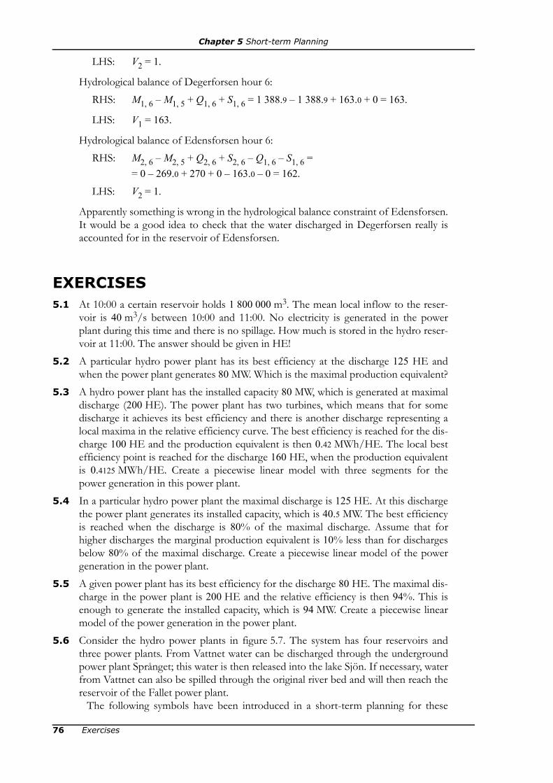
Chapter 5 Short-term Planning
LHS: V2 = 1.
Hydrological balance of Degerforsen hour 6:RHS: M1, 6 – M1, 5 + Q1, 6 + S1, 6 = 1 388.9 – 1 388.9 + 163.0 + 0 = 163.
LHS: V1 = 163.
Hydrological balance of Edensforsen hour 6:RHS: M2, 6 – M2, 5 + Q2, 6 + S2, 6 – Q1, 6 – S1, 6 =
= 0 – 269.0 + 270 + 0 – 163.0 – 0 = 162.LHS: V2 = 1.
Apparently something is wrong in the hydrological balance constraint of Edensforsen.It would be a good idea to check that the water discharged in Degerforsen really isaccounted for in the reservoir of Edensforsen.
EXERCISES5.1 At 10:00 a certain reservoir holds 1 800 000 m3. The mean local inflow to the reser-
voir is 40 m3/s between 10:00 and 11:00. No electricity is generated in the powerplant during this time and there is no spillage. How much is stored in the hydro reser-voir at 11:00. The answer should be given in HE!
5.2 A particular hydro power plant has its best efficiency at the discharge 125 HE andwhen the power plant generates 80 MW. Which is the maximal production equivalent?
5.3 A hydro power plant has the installed capacity 80 MW, which is generated at maximaldischarge (200 HE). The power plant has two turbines, which means that for somedischarge it achieves its best efficiency and there is another discharge representing alocal maxima in the relative efficiency curve. The best efficiency is reached for the dis-charge 100 HE and the production equivalent is then 0.42 MWh/HE. The local bestefficiency point is reached for the discharge 160 HE, when the production equivalentis 0.4125 MWh/HE. Create a piecewise linear model with three segments for thepower generation in this power plant.
5.4 In a particular hydro power plant the maximal discharge is 125 HE. At this dischargethe power plant generates its installed capacity, which is 40.5 MW. The best efficiencyis reached when the discharge is 80% of the maximal discharge. Assume that forhigher discharges the marginal production equivalent is 10% less than for dischargesbelow 80% of the maximal discharge. Create a piecewise linear model of the powergeneration in the power plant.
5.5 A given power plant has its best efficiency for the discharge 80 HE. The maximal dis-charge in the power plant is 200 HE and the relative efficiency is then 94%. This isenough to generate the installed capacity, which is 94 MW. Create a piecewise linearmodel of the power generation in the power plant.
5.6 Consider the hydro power plants in figure 5.7. The system has four reservoirs andthree power plants. From Vattnet water can be discharged through the undergroundpower plant Språnget; this water is then released into the lake Sjön. If necessary, waterfrom Vattnet can also be spilled through the original river bed and will then reach thereservoir of the Fallet power plant.
The following symbols have been introduced in a short-term planning for these
76 Exercises

Chapter 5 Short-term Planning
power plants:Indices for power plants and reservoirs: Vattnet/Språnget 1, Forsen 2, Sjön 3, Fallet 4.
γi = expected future production equivalent for water stored in reservoir i, i = 1, 2, 3, 4,
λt = expected electricity price during hour t, t = 1, …, 24,λ25 = expected electricity price after the end of the planning period,
Mi, 0 = contents of reservoir i at the beginning of the planning period, i = 1, 2, 3, 4, Mi, t = contents of the reservoir i at the end of hour t, i = 1, 2, 3, 4, t = 1, …, 24,μi, j = marginal production equivalent for power plant i, segment j, i = 1, 2, 3, 4,
j = 1, 2,Qi, j, t = discharge in power plant i, segment j, during hour t,
i = 1, 2, 3, 4, j = 1, 2, t = 1, …, 24.Si, t = spillage from reservoir i during hour t, i = 1, 2, 3, 4, t = 1, …, 24,Vi, t = local inflow to reservoir i during hour t, i = 1, 2, 3, 4, t = 1, …, 24.
a) Which symbols denote optimisation variables and parameters respectively?b) Formulate the objective function if the purpose of the planning is to maximise theincome of generated hydro power plus the value of stored water.c) Formulate the hydrological constraints of this system. The delay time between thepower plants can be neglected.
Sjön
Fallet
Språnget
Forsen
Vattnet
Figure 5.7 The river system in exercise 5.6.
Exercises 77

Chapter 5 Short-term Planning
5.7 AB Vattenkraft owns two hydro power plants, located as shown in figure 5.8. Data ofthe hydro power plants are given in table 5.13. The company expects that the electric-ity price the coming five hours will be 200, 210, 210, 220 and 210 SEK/MWh respec-tively. After this period the average electricity price is estimated to 200 SEK/MWhand stored water is assumed to be used for generation at best efficiency. The reser-voirs are half-filled at the beginning of the planning period.
Since the river where the power plants are located is an important breeding area forsalmon, the Environment Court has judged that the company must build fish ladderswhich allow fish to pass the dams. The minimum water flow in each fish ladder mustbe 1 m3/s; this water can thus not be used for power generation. Moreover, the Envi-ronment Court has decided that for tourism reasons the river flow in the river sec-tions downstream each power plant may not be less than 10 m3/s.
Formulate the planning problem of AB Vattenkraft as a an LP problem. The waterdelay time between the power plants can be neglected.
5.8 The thermal power plant Flisinge is fuelled by biomass. The fuel costs 200 ¤/m3 andhas a density of 400 kg/m3. The heat contents of the fuel is 5 MWh/ton and the effi-
Table 5.13 Data of the hydro power plants in exercise 5.7.
Power plantMaximal reservoir
contents [HE]
Marginal production equivalents [MWh/HE]
Local inflow [m3/s]
Språnget 10 000 0.36 for discharges between 0 and 300 HE0.32 for discharges between 300 and 400 HE 150
Fallet 2 000 0.48 for discharges between 0 and 100 HE0.46 for discharges between 100 and 200 HE 10
Språnget
FalletFish ladder
Fish ladder
Figure 5.8 The hydro power plants in exercise 5.7.
78 Exercises
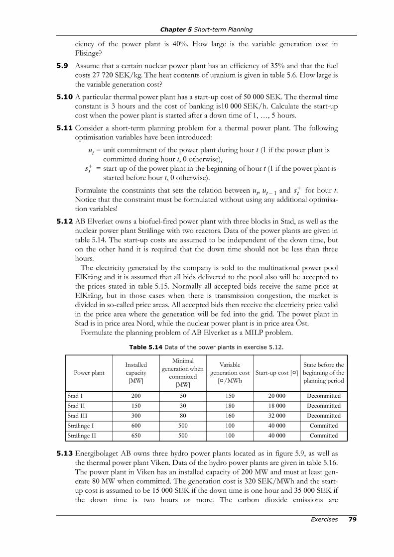
Chapter 5 Short-term Planning
ciency of the power plant is 40%. How large is the variable generation cost inFlisinge?
5.9 Assume that a certain nuclear power plant has an efficiency of 35% and that the fuelcosts 27 720 SEK/kg. The heat contents of uranium is given in table 5.6. How large isthe variable generation cost?
5.10 A particular thermal power plant has a start-up cost of 50 000 SEK. The thermal timeconstant is 3 hours and the cost of banking is10 000 SEK/h. Calculate the start-upcost when the power plant is started after a down time of 1, …, 5 hours.
5.11 Consider a short-term planning problem for a thermal power plant. The followingoptimisation variables have been introduced:
ut = unit commitment of the power plant during hour t (1 if the power plant is committed during hour t, 0 otherwise),
= start-up of the power plant in the beginning of hour t (1 if the power plant is started before hour t, 0 otherwise).
Formulate the constraints that sets the relation between ut, ut – 1 and for hour t.Notice that the constraint must be formulated without using any additional optimisa-tion variables!
5.12 AB Elverket owns a biofuel-fired power plant with three blocks in Stad, as well as thenuclear power plant Strålinge with two reactors. Data of the power plants are given intable 5.14. The start-up costs are assumed to be independent of the down time, buton the other hand it is required that the down time should not be less than threehours.
The electricity generated by the company is sold to the multinational power poolElKräng and it is assumed that all bids delivered to the pool also will be accepted tothe prices stated in table 5.15. Normally all accepted bids receive the same price atElKräng, but in those cases when there is transmission congestion, the market isdivided in so-called price areas. All accepted bids then receive the electricity price validin the price area where the generation will be fed into the grid. The power plant inStad is in price area Nord, while the nuclear power plant is in price area Öst.
Formulate the planning problem of AB Elverket as a MILP problem.
5.13 Energibolaget AB owns three hydro power plants located as in figure 5.9, as well asthe thermal power plant Viken. Data of the hydro power plants are given in table 5.16.The power plant in Viken has an installed capacity of 200 MW and must at least gen-erate 80 MW when committed. The generation cost is 320 SEK/MWh and the start-up cost is assumed to be 15 000 SEK if the down time is one hour and 35 000 SEK ifthe down time is two hours or more. The carbon dioxide emissions are
Table 5.14 Data of the power plants in exercise 5.12.
Power plantInstalled capacity [MW]
Minimal generation when
committed [MW]
Variable generation cost
[¤/MWhStart-up cost [¤]
State before the beginning of the planning period
Stad I 200 50 150 20 000 DecommittedStad II 150 30 180 18 000 DecommittedStad III 300 80 160 32 000 DecommittedStrålinge I 600 500 100 40 000 CommittedStrålinge II 650 500 100 40 000 Committed
st+
st+
Exercises 79

Chapter 5 Short-term Planning
0.33 tonnes/MWh. During start-up the emissions are 15 tonnes if the down time wasone hour and 36 tonnes otherwise. Energibolaget AB has an environmental policywhich states that they should never emit more than 850 tonnes carbon dioxide a day.
Currently Energibolaget AB sells all of its generation to AB Elhandel. The con-tracted sales are 350 MWh/h between 8 am and 5 pm, and 150 MWh/h during theremaining hours.
Energibolaget AB now wants to plan the operation for the next 24 hours. Formulatethe planning problem of the company as a n MILP problem. Assume that the electric-ity price after the planning period will be 330 SEK/MWh and that stored water willbe used for electricity generation at the maximal marginal production equivalent. Thereservoirs are filled to 75% at the beginning of the planning period. The water delaytime can be neglected.
FURTHER READING• J. F. Bard, “Short-term Scheduling of Thermal-electric Generators Using Lagrangian Relaxation”,
Operations Research, Vol. 36, No. 5, September-October 1988. — Example of thermal power plant mod-els.
• G. W. Chang, Y. D. Tsai, C. Y. Lai & J. S. Chung, “A Practical Mixed Integer Linear ProgrammingBased Approach for Unit Commitment”, 2004 IEEE Power Engineering Society General Meeting Proceed-ings, Denver 2004. — Example of thermal power plant models.
Table 5.15 Expected power pool prices in exercise 5.12.
Hour 1 2 3 4 5 6 7 8 9 10 11 12
Price area Nord 116 118 108 108 115 160 210 290 291 291 290 273Price area Öst 116 118 108 108 115 130 136 148 148 150 145 141
Hour 13 14 15 16 17 18 19 20 21 22 23 24
Price area Nord 272 163 138 137 140 142 137 134 130 120 98 105Price area Öst 141 139 138 137 140 142 137 134 130 120 98 105
Forsen
Strömmen
Ån
Thermal powerplant Viken
Figure 5.9 The power plants in exercise 5.13.
80 Further Reading

Chapter 5 Short-term Planning
• O. Nilsson, L. Söder & D. Sjelvgren, “Integer Modelling of Spinning Reserve Requirements in ShortTerm Scheduling of Hydro Systems”, IEEE Transactions on Power Systems, Vol. 13, No. 3, August1998 — Example of a mixed integer linear model for hydro power.
• A. J. Wood & B. F. Wollenberg, Power Generation Operation and Control, second edition, John Wiley &Sons, 1996 — General textbook which describes both hydro power and thermal power plants.
Table 5.16 Data of the hydro power plants in exercise 5.13.
Power plantMaximal reservoir
contents [m3]
Marginal production equivalents [MWh/HE]
Local inflow [m3/s]
Forsen 7 200 000 0.28 for discharges between 0 and 150 HE0.21 for discharges between 150 and 310 HE 125
Ån 2 880 000 0.42 for discharges between 0 and 200 HE0.32 for discharges between 200 and 400 HE 175
Strömmen 3 600 000 0.34 for discharges between 0 and 180 HE0.28 for discharges between 180 and 370 HE 30
Further Reading 81

82

Chapter 6
SIMULATION OFELECTRICITY MARKETS
There are many contexts in which there is a need to predict the long-term behaviour of an electric-ity market. The most simple alternative is then to use rough estimates (as for example the simpleprice model in chapter 3), but to perform a deeper analysis it is necessary to simulate the electricitymarket. The starting point when simulating an electricity market is to make assumptions about theresources of the system (for example generation and transmission capacity), the demand and theregulation controlling the electricity trade. Given these inputs, we try to predict the function of theelectricity market.
The choice of model and method in an electricity market simulation is of course depending onthe factors which are to be studied. If we for example want to study the impact of various environ-ment regulations then it is necessary to somehow model how the players of the electricity marketrespond to the various market designs. There is a wide range of possible models—in this compen-dium we will have to restrict ourselves to the most basic models for electricity market simulation.
We will describe two simulation methods. The first is probabilistic production cost simulation(PPC). This method is limited to a rather simplistic model of the electricity market, as it is basedon analytical calculations. The other method is Monte Carlo simulation, which is a more versatilesimulation method—the only limitation to the possible models to be simulated by Monte Carlomethods is the computation capacity of the computer used for the simulation. A completedescription of Monte Carlo simulation would not fit into this compendium and we will thereforeonly provide an introduction to the subject.
6.1 PROBLEM DESCRIPTIONBefore we address the actual simulation methods it is appropriate to investigate what kind of prob-lems can be analysed by an electricity market simulation. The objective of simulating an electricitymarket is as mentioned above to predict the behaviour of the electricity market given a set of con-ditions (inputs). Let us introduce the designation scenario for a given situation, where available re-sources, demand as well as all other factors influencing the electricity market are known. As allthese conditions vary more or less randomly in an electricity market, there will in general be an in-finite number of possible scenarios. To predict the behaviour of the electricity market we wouldtherefore like to know how the electricity market will work in each scenario.
The conditions in a particular scenario is described by a number of parameters, which we mayrefer to as scenario parameters. Each scenario parameter is a random variable, the probability distribu-tion of which is known (consequently, the probability distribution is an input to the simulation).
6.1 Problem Description 83

Chapter 6 Simulation of Electricity Markets
Exactly which scenario parameters we have depend on which model we have chosen. For themoment, it is sufficient that we collect all scenario parameters in the random vector Y.
The simulation also requires a mathematical model of the electricity market. In this model thereare several constants, the value of which is the same in all scenarios. We refer to these constants asmodel constants, and as the scenario parameters, they constitute inputs for the simulation. We maysay that the model constants in combination with the structure of the mathematical model forms amathematical function, g, which shows how the electricity market responds to a particular sce-nario. In many cases the electricity market is so complex that the function g only can be definedindirectly, for example from the solution of an optimisation problem (we will see an example ofthis later in this section).
The outputs of the simulation shows how the electricity market behaves in each possible sce-nario. It is possible to study several characteristics, as for example resource usage and prices.Depending on which properties we want to study, we will have to define a number of result varia-bles. For the moment, we collect all result variables in a random vector, X. As the scenario param-eters, the result variables are random variables, but the major difference is that the probability dis-tribution of the result variables is unknown prior to the simulation.
Thus, the relation between the scenario parameters and the result variables is given by the math-ematical model, i.e.,
X = g(Y). (6.1)To predict the behaviour of the electricity market is equivalent to calculating the probability distri-bution of the result variables. In many cases it is inconvenient to consider all possible events in de-tail (i.e., to consider all possible outcomes of the result variables). It is more appropriate to usesimple, easily understood measures, which summarises the most important characteristics of anelectricity market. Most straightforward is to define a number of key values—system indices—whichcan be used for comparison of alternative electricity markets. The system indices are in practicestatistical measures (generally expectation values) of the result variables. Therefore, we may saythat the actual objective of an electricity market simulation is to determine
E[X] = E[g(Y)]. (6.2)Below we will give an example of how an electricity market model can be designed and how the re-sults of a simulation can be used for electricity market analysis.
6.1.1 Example of an Electricity Market ModelThe electricity market model should, as described above, describe how the electricity market re-sponds to a particular scenario. In many cases this means that we formulate an optimisation prob-lem corresponding to the short-term planning problem the players of the electricity market wouldhave to solve. The model suggested here is a multi-area model intended for Monte Carlo simula-tion. (However, as we will see later in this chapter, the model of probabilistic production cost sim-ulation is a special case of the multi-area model.) In a Monte Carlo simulation a number of ran-domly chosen scenarios are investigated and it is observed how the electricity market behaves inthose (see section 6.3). These observations are obtained by analysing the solution to the optimisa-tion problem. A Monte Carlo simulation can require that a large number of scenarios are consid-ered; therefore, it is desirable that each optimisation problem can be solved as quickly as possible.In practice this means that we should minimise the number of variables in the problem.
One way to reduce the number of variables, while still modelling different power plants andtransmission losses is to use a multi-area model. The power system is then divided in several areasconnected transmission lines (see figure 6.1). All power plants and all consumption must belocated in a specific area. In the model we assume that there is perfect competition and that all
84 6.1 Problem Description

Chapter 6 Simulation of Electricity Markets
players have perfect information. Moreover, we make the following assumption of the modelledplayers:
•Thermal power plants. The thermal power plants are modelled by a certain avail-able generation capacity and a cost function. As we learned in section 5.3 it is neces-sary to use integer variables to model the start-up costs of a thermal power plant.Therefore we neglect the start-up costs, because including them would significantlyincrease the solution time of the multi-area problem. Hence, the cost function is justfunction of the generation cost. This function could be quadratic, i.e.,
CGg(Gg) = αGg + βGgGg + (6.3)
Several thermal power plants located in the same area might be combined into anequivalent power plant.
•Non-dispatchable power plants. By non-dispatchable power plants we refer tosuch power plants where the generation capacity depend on some factor beyond hu-man control. Examples of non-dispatchable units are wind power plants, hydro powerplants without reservoirs and photovoltaics. The designation non-dispatchable is actu-ally slightly misleading, because it is always possible to reduce the generation of thesepower plants (for example by spilling water in a hydro power plant). However, in prac-tice this is only done when absolutely necessary to maintain safe operation of thepower system, as the variable generation cost in the non-dispatchable units generally isso low that it is optimal to run these units at the maximal available capacity.
In the multi-area model we assume that the generation cost in the non-dispatchablepower plants is negligible. The available generation capacity in all non-dispatchableunits is summed per area.
•The grid. In the model the grid is only represented by the interconnections betweenthe areas. Between two areas there can only be one interconnection in each directionand these interconnections are characterised by a certain available transmission capac-ity and a certain loss function. The loss function can be quadratic, i.e.,
Ln, m(Pn, m) = βLn, mPn, m + (6.4)
We assume that the players of the electricity market have full control of the power
Figure 6.1 The power system in a multi-area problem.
Area 1
Area 2
Area 3
γGgGg2.
γLn m, Pn m,2 .
6.1 Problem Description 85

Chapter 6 Simulation of Electricity Markets
flow between the areas, as long as the transmission capacity is not exceeded.•Load. In the model it is assumed that the load is not price sensitive. Hence, the load
can be modelled as a certain demand in each area. As there are no guarantee that therealways is sufficient generation capacity, we will have to introduce a possibility to dis-connect a part of the load. This possibility is represented in the model by a special var-iable for load shedding (unserved power).
Mathematical Formulation
The multi-area problem can in words be expressed asminimise generation cost + penalty cost of load shedding, (6.5)
subject to load balance in each area(i.e., generation + import = load – load shedding + export), (6.5a)
limitations in generation and transmission capacity. (6.5b)
The following parameters are included in the multi-area problem:CGg = cost function for generation in thermal power plant g,CUn = penalty cost for unserved load in area n,
G = set of thermal power plants g,Gn = set of thermal power plants g located in area n,
= maximal generation in thermal power plant g,Dn = load in area n,
Ln, m = loss function for transmission from area n to area m,N = set of areas n,P = set of interconnections (n, m),
Pn←m = set of areas m capable of exporting to area n,Pn→m = set of areas m capable of importing from area n,
= maximal non-dispatchable generation in area n.The following optimisation variables are included in the multi-area problem:
Gg = generation in thermal power plant g,Pn, m = transmission from area n to area m,
Un = unserved power in area n,Wn = non-dispatchable generation in area n.
Using these symbols we get the following mathematical formulation of the multi-area problem:
minimise (6.6)
subject to
∀ n ∈ N, (6.6a)
0 ≤ Gg ≤ ∀ g ∈ G, (6.6b)0 ≤ Pn, m ≤ ∀ (n, m) ∈ P, (6.6c)0 ≤ Un ≤ Dn, ∀ n ∈ N, (6.6d)0 ≤ Wn ≤ ∀ g ∈ N. (6.6e)
Notice that the objective function has to include a penalty cost for unserved load, because other-
Gg
Wn
CGg Gg( ) CUn Un( )n N∈∑+
g G∈∑
Gg Wn Pm n, Lm n, Pm n,( )–( )m Pn←m∈
∑+ +g Gn∈
∑ Dn Un– Pn m, ,m Pn→m∈
∑+=
Gg,
Pn m, ,
Wn,
86 6.1 Problem Description
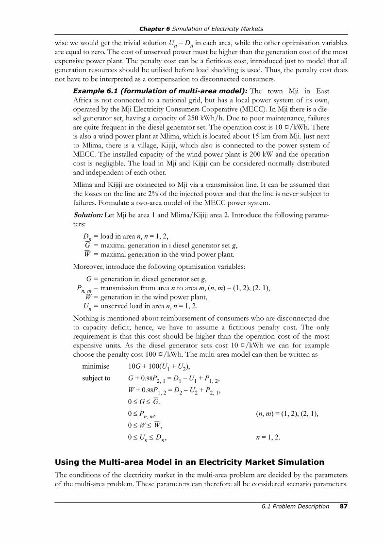
Chapter 6 Simulation of Electricity Markets
wise we would get the trivial solution Un = Dn in each area, while the other optimisation variablesare equal to zero. The cost of unserved power must be higher than the generation cost of the mostexpensive power plant. The penalty cost can be a fictitious cost, introduced just to model that allgeneration resources should be utilised before load shedding is used. Thus, the penalty cost doesnot have to be interpreted as a compensation to disconnected consumers.
Example 6.1 (formulation of multi-area model): The town Mji in EastAfrica is not connected to a national grid, but has a local power system of its own,operated by the Mji Electricity Consumers Cooperative (MECC). In Mji there is a die-sel generator set, having a capacity of 250 kWh/h. Due to poor maintenance, failuresare quite frequent in the diesel generator set. The operation cost is 10 ¤/kWh. Thereis also a wind power plant at Mlima, which is located about 15 km from Mji. Just nextto Mlima, there is a village, Kijiji, which also is connected to the power system ofMECC. The installed capacity of the wind power plant is 200 kW and the operationcost is negligible. The load in Mji and Kijiji can be considered normally distributedand independent of each other.Mlima and Kijiji are connected to Mji via a transmission line. It can be assumed thatthe losses on the line are 2% of the injected power and that the line is never subject tofailures. Formulate a two-area model of the MECC power system.Solution: Let Mji be area 1 and Mlima/Kijiji area 2. Introduce the following parame-ters:
Dn = load in area n, n = 1, 2,= maximal generation in i diesel generator set g, = maximal generation in the wind power plant.
Moreover, introduce the following optimisation variables:G = generation in diesel generator set g,
Pn, m = transmission from area n to area m, (n, m) = (1, 2), (2, 1),W = generation in the wind power plant,
Un = unserved load in area n, n = 1, 2.Nothing is mentioned about reimbursement of consumers who are disconnected dueto capacity deficit; hence, we have to assume a fictitious penalty cost. The onlyrequirement is that this cost should be higher than the operation cost of the mostexpensive units. As the diesel generator sets cost 10 ¤/kWh we can for examplechoose the penalty cost 100 ¤/kWh. The multi-area model can then be written as
minimise 10G + 100(U1 + U2),subject to G + 0.98P2, 1 = D1 – U1 + P1, 2,
W + 0.98P1, 2 = D2 – U2 + P2, 1,0 ≤ G ≤
0 ≤ Pn, m, (n, m) = (1, 2), (2, 1),0 ≤ W ≤
0 ≤ Un ≤ n = 1, 2.
Using the Multi-area Model in an Electricity Market Simulation
The conditions of the electricity market in the multi-area problem are decided by the parametersof the multi-area problem. These parameters can therefore all be considered scenario parameters.
GW
G,
W,Dn,
6.1 Problem Description 87
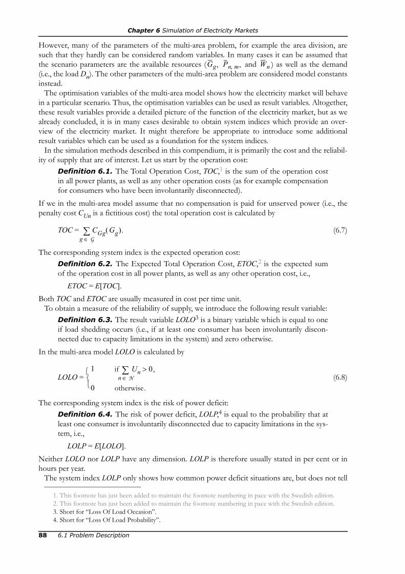
Chapter 6 Simulation of Electricity Markets
However, many of the parameters of the multi-area problem, for example the area division, aresuch that they hardly can be considered random variables. In many cases it can be assumed thatthe scenario parameters are the available resources ( and ) as well as the demand(i.e., the load Dn). The other parameters of the multi-area problem are considered model constantsinstead.
The optimisation variables of the multi-area model shows how the electricity market will behavein a particular scenario. Thus, the optimisation variables can be used as result variables. Altogether,these result variables provide a detailed picture of the function of the electricity market, but as wealready concluded, it is in many cases desirable to obtain system indices which provide an over-view of the electricity market. It might therefore be appropriate to introduce some additionalresult variables which can be used as a foundation for the system indices.
In the simulation methods described in this compendium, it is primarily the cost and the reliabil-ity of supply that are of interest. Let us start by the operation cost:
Definition 6.1. The Total Operation Cost, TOC,1 is the sum of the operation costin all power plants, as well as any other operation costs (as for example compensationfor consumers who have been involuntarily disconnected).
If we in the multi-area model assume that no compensation is paid for unserved power (i.e., thepenalty cost CUn is a fictitious cost) the total operation cost is calculated by
TOC = (6.7)
The corresponding system index is the expected operation cost:Definition 6.2. The Expected Total Operation Cost, ETOC,2 is the expected sumof the operation cost in all power plants, as well as any other operation cost, i.e.,
ETOC = E[TOC].
Both TOC and ETOC are usually measured in cost per time unit.To obtain a measure of the reliability of supply, we introduce the following result variable:
Definition 6.3. The result variable LOLO3 is a binary variable which is equal to oneif load shedding occurs (i.e., if at least one consumer has been involuntarily discon-nected due to capacity limitations in the system) and zero otherwise.
In the multi-area model LOLO is calculated by
LOLO = (6.8)
The corresponding system index is the risk of power deficit:Definition 6.4. The risk of power deficit, LOLP,4 is equal to the probability that atleast one consumer is involuntarily disconnected due to capacity limitations in the sys-tem, i.e.,
LOLP = E[LOLO].
Neither LOLO nor LOLP have any dimension. LOLP is therefore usually stated in per cent or inhours per year.
The system index LOLP only shows how common power deficit situations are, but does not tell
1. This footnote has just been added to maintain the footnote numbering in pace with the Swedish edition.2. This footnote has just been added to maintain the footnote numbering in pace with the Swedish edition.3. Short for “Loss Of Load Occasion”.4. Short for “Loss Of Load Probability”.
Gg, Pn m, , Wn
CGg Gg( ).g G∈∑
1
0⎩⎨⎧ if Un 0,>
n N∈∑
otherwise.
88 6.1 Problem Description

Chapter 6 Simulation of Electricity Markets
us anything about the size of the problem; we have a power deficit even if just a 60 W light bulbhas been disconnected. To get a measure of the extent of a power deficit situation we make thefollowing definitions:
Definition 6.5. The unserved energy, ENS,5 is the energy that could not be deliv-ered due to capacity limitations in the power system.
In the multi-area model ENS is calculated by
ENS = (6.9)
The corresponding system index is the expected unserved energy:Definition 6.6. The expected unserved energy, EENS,6 is the expected energy thatcould not be delivered due to capacity limitations in the power system, i.e.,
EENS = E[ENS].
Both ENS and EENS are usually measured as energy per time unit.It must be observed that there is no simple relation between LOLP and EENS! It is not uncom-
mon to believe that the unserved energy equals the LOLP multiplied by the maximal load or theLOLP multiplied by the average load. This could be the case at some occasions, bute it is abso-lutely no general rule (cf. exercise 6.7).
Example 6.2 (scenario parameters and result variables in a multi-area model): Consider the multi-area model in example 6.1. Assume that theobjective of the simulation is to determine the system indices ETOC and LOLP. Whichscenario parameters are included in the model? Which result variables are relevant andhow can values of those be obtained?Solution: The scenario parameters are the quantities that can vary randomly andwhich determine the conditions for operation of the system. In this case we have themaximal generation capacity in the power plants, and as well as the load in eacharea, D1 and D2.The relevant result variables in this simulation are TOC and LOLO, because the systemindices ETOC and LOLP are the expectation values of these result variables. For a par-ticular scenario, we can solve the multi-area problem from example 6.1 and then cal-culate the values of the result variables according to
TOC = 10G,
LOLO =
6.1.2 Examples of ApplicationsElectricity market simulation can be used to study how an electricity market can be expected to be-have with various prerequisites. By comparing the results it is thus possible to conclude whether ornot an investment is profitable, or which arrangement of the electricity trading will be best toachieve a specified goal. In this section, we will give some short examples of how the results of anelectricity market simulation will be used.
5. Short for “Energy Not Served”.6. Short for “Expected Energy Not Served”. Sometimes the abbreviation UE (for “Unserved Energy”) is
used.
Un.n N∈∑
G W,
0
1⎩⎨⎧ om U1 U2+ 0,=
om U1 U2 0.>+
6.1 Problem Description 89

Chapter 6 Simulation of Electricity Markets
The Value of an Investment
To determine the value of an investment it is necessary to find out how the above described sys-tem indices are affected by the investment. This requires at least two simulations: one simulationof the system before the investment is made and then a simulation of how the system behaves af-ter the investment. The value of the investment is the difference of the system indices between thetwo simulations. The value of the investment can then be compared to the cost of the investment.The cost of the investment must consider interest rates and depreciation time. A simple way to ac-complish this is to use the so-called annuity formula:
AC = (6.10)
where
AC = annual cost [¤],I = investment cost [¤],r = real rate of interest [%],n = depreciation time [years].
The annuity formula distributes the initial investment cost as an annual amount over the wholedeprecation time. If the annual amounts are summed, the result is higher than the initial invest-ment (if r > 0), due to the interest rate.
Example 6.3 (the value of a transmission line): Consider an electricitymarket divided into two regions. In region A the load is 150 kWh/h during peak peri-ods and 100 kWh/h otherwise. In region B the corresponding values are 100 kWh/hand 50 kWh/h respectively. Workdays between 6 a.m. and 8 p.m., and weekendsbetween 10 a.m. and 5 p.m. are considered peak periods. In region A there are twodiesel generator sets with operation costs 10 ¤/kWh, and in region B there is one die-sel generator set with an operation cost of 12 ¤/kWh. All units have an availability of90% and a capacity of 100 kWh/h.At present time the two regions are not interconnected; however, the construction ofa transmission line is discussed. The transmission line can be considered loss free andhaving an unlimited capacity. The cost of the project, including capital costs andannual maintenance, is estimated to 275 000 ¤/year. Is it profitable to build the trans-mission line?Solution: Two cases have to be simulated: the current situation with two separate sys-tem as well as the situation when the two regions are interconnected and can betreated as a single system. Later in this chapter we will describe methods to performthese simulations. For the moment it is sufficient to study the result, which are shownin the table below.
By comparing the two cases we can find that the transmission line results in an annualcost saving of 260 000 ¤/year, due to the reduced operation costs. If this was the only
Table 6.1 System index with and without the transmission line.
System index No transmission line
With the transmission line
ETOC [¤/h] 2 002.50 1 972.80
LOLPA [%] 1014.5
LOLPB [%] 10
I r 100⁄1 1 r 100⁄+( ) n––------------------------------------------- ,⋅
90 6.1 Problem Description
Chapter 6 Simulation of Electricity Markets
criteria to be evaluated the transmission line would seem unprofitable. However, with-out the transmission line the risk of power deficit for the market as a whole is 19%,7which is reduced to 14.5% if the transmission line is built. If the increased reliability isvalued to at least 15 000 ¤/year then the transmission line is profitable. If the reduc-tion in loss of load probability is less than that then the transmission line should notbe built.
The Capacity Credit of a Power Plant
If the available generation capacity is less than the power demand then some consumption has tobe disconnected. The risk of power deficit, LOLP, is in the normal case very low, but it can neverbe reduced to zero, i.e., LOLP > 0If we have a certain system and build another power plant, theprobability of consumers having to be disconnected will decrease, as the generation capacity of thesystem increases. The ability of a power plant to increase the reliability of supply is referred to asits capacity credit. Of course, also the existing power plants in system have a capacity credit, becauseif they were removed the LOLP of the system would increase.
The capacity credit can be expressed in several ways. Two possible definitions are the following:Definition 6.7. The capacity credit of a power plant g expressed as equivalent firmpower is measured by comparing the ability of the power plant to decrease the LOLPto the corresponding ability of a 100% reliable power plant. Including the power plantg the system has certain risk of power deficit, LOLP′. Excluding power plant g andreplacing it by a 100% reliable power plant with the installed capacity yieldsanother risk of power deficit, LOLP′′. If LOLP′ = LOLP′′ then the power plants havethe same ability to decrease the risk of power deficit, and then it said that power plantg has the capacity credit expressed as equivalent firm power.Definition 6.8. The capacity credit of a power plant g expressed as equivalent loadincrease is measured by studying the ability of power plant g to prevent the risk ofpower deficit from increasing as the load increases. A given mean load μD yields a cer-tain risk of power deficit LOLP′ when power plant g is excluded from the system. Ifpower plant g is included and the mean load is increased by Δ then the risk of powerdeficit becomes LOLP′′. If LOLP′ = LOLP′′ then the power plant has prevented therisk of power deficit to increase for this load increase, and then it is said that powerplant g has the capacity credit Δ expressed as an equivalent, equally distributed loadincrease.
There are many possible variations of these definitions. It is for example possible to replace the100% reliable power plant in definition 6.7 by a standard power plant having a availability8 lessthan 100%. In definition 6.8 we could have another distribution of the load increase, for examplea load which is increasing more during peak load periods.
Example 6.4 (capacity credit): Table 6.2 shows how the LOLP is changed in acertain system when the load increases and new power plants are added. Determinethe capacity credit of the wind power expressed as equivalent firm power and asequivalent load increase. Solution: 100 MW wind power has been added in variant 1 and this results in thesame risk of power deficit as in variant 2, where 22.2 MW of firm power has been
7. To obtain this figure it is necessary to consider that LOLPA is 19% during peak periods but only 1% other-wise, whereas LOLPB is the same regardless of which time it is. The probability of all consumers in bothregions being supplied is therefore 0.5·0.81·0.9 + 0.5·0.99·0.9 = 81%.
8. See section 6.2.3 for a more thorough description of the reliability of a power plant.
G
G
6.1 Problem Description 91

Chapter 6 Simulation of Electricity Markets
added instead. This means, according to definition 6.7, that in this system 100 MWwind power has the capacity credit 22.2 MW expressed as equivalent firm power.In variant 3 the mean load has increased to 522.4 MW, but the standard deviation ofthe load remains the same, which means that the load increase is equally large at alltimes. The LOLP is the same as in the original system, thanks to the 100 MW windpower which has been added. According to definition 6.8, we can conclude that100 MW wind power in this system has the capacity credit 22.4 expressed as an evenlydistributed load increase.In variant 4 the mean load has increased to 514.0 MW. However, in this case the loadincrease is larger during peak load periods, which is reflected by the fact that thestandard deviation of the load has increased to 105 MW. The LOLP is the same as inthe original system, thanks to the 100 MW wind power which has been added. We canconclude that 100 MW wind power in this system has the capacity credit 14.0expressed as an unevenly distributed load increase.
It can be noted that the example above counters the wide-spread misconception that “windpower has no capacity credit because it is not always windy”. It is correct that the wind power hasa lower capacity credit than the same installed capacity in a power plant which is not weatherdependent, but as the example shows still wind power has the ability to decrease the risk of powerdeficit.
6.2 PROBABILISTIC PRODUCTION COST SIMULATION
In this section we will present the method of probabilistic production cost simulation (PPC). Themethod, which was developed in the late 1960s, can be used to simulate simple electricity markets.The main concept of the method is to use such a simple electricity market model that all scenarioparameters can be combined into a single one-dimensional probability distribution. From this dis-tribution it is possible to analytically calculate system indices as ETOC and LOLP.
In order to avoid too complex calculations it is necessary to make some simplifying assumptions.The most important assumption is to neglect all correlations9 between random variables, as for
Table 6.2 Data of various system configurations in example 6.4.
Original system Variant 1 Variant 2 Variant 3 Variant 4
Load (normally distributed) [MW]Mean 500.0 500.0 500.0 522.3 514.0Standard deviation 100.0 100.0 100.0 100.0 105.0
Installed capacity in different power plants [MW]Coal condensing (95% availability) 5 × 200 5 × 200 5 × 200 5 × 200 5 × 200Wind powera
a. At any given moment (independent of the load) the probability that the wind power can generate installed capacity is assumed to be 10%; the probability of half the installed capacity being available is 40% and the probability of no generation at all is 50%. This means that the wind power in aver-age generates 30% of installed capacity.
0 100 0 100 100Firm power (100% availability) 0 0 22.2 0 0
LOLP [%] 0.0787 0.0537 0.0537 0.0787 0.0787
92 6.2 Probabilistic Production Cost Simulation

Chapter 6 Simulation of Electricity Markets
example load and available generation capacity. This assumption is so fundamental for probabilis-tic production cost simulation that we state it formally:
Assumption 6.9. All random variables in a probabilistic production cost simulationare assumed to be independent!
In practice it is sometimes possible to consider correlated variables in a simplified manner, whichwill be shown in the subsection on simulation of wind power.
Another simplification in PPC is that the transmission grid is more or less entirely neglected.The power system model in a probabilistic production cost simulation may therefore be seen as avariant of the electricity market model from section 6.1.1, but with just one area.
The description of probabilistic production cost simulation starts by a compilation of the mostbasic calculations in the method. Then we show how to obtain the necessary models of load andsimple power plants. Later we add more advanced models of wind power and dispatchable hydropower. Finally we also describe a method to simplify the calculation of the LOLP by using the so-called normal approximation.
6.2.1 Basic PrinciplesAssume that we know the duration curve of theload in a system, 10 and that this loadmust be supplied by a single power plant. Thepower plant is however not completely reliable;there is a possibility that the plant is failing andcan not generate any electric power at all. Theprobability of this is called the availability. In thispower plant we have the availability p1 and theoperation cost β1. By comparing the load dura-tion curve and the generation duration curve ofthe power plant it is comparatively easy to calcu-late the system reliability and operation cost, asshown in the following example:
Example 6.5. In a simple system theload is constantly 200 kW. The system issupplied by a 200 kW power plant having an availability of 80% and the operationcost 1 ¤/kWh. Calculate the EENS, LOLP and ETOC of the system.Solution: Since the load is constant the probability is 1 that the load exceeds the levelx if x < 200 kW and 0 if x ≥ 200 kW, which results in the duration curve shown infigure 6.2. When the power plant is available, a probability which is stated to 80%, itwill generate enough to meet the load. The duration curve of the power generation istherefore such that the probability is 1 that the generation exceeds the level x if x isnegative. However, negative generation is obviously not possible, so that part of theduration curve is not interesting. The probability is 0.8 that x is exceeded if x is largerthan or equal to zero but less than 200 kW and the probability is 0 then x ≥ 200 kW.This duration curve is illustrated by the shadowed part of the figure.From the figure we can directly obtain the most important system indices. The
9. See appendix C.10. Definitions of duration curves and other important notions concerning random variables are found in
appendix C.
kW
x
100 200 300
1
0.6
0.8
0.4
0.2
F0
400 500
EENS
Figure 6.2 Calculation of system indicesdirectly from the load durationcurve.
F0 x( ) ,
6.2 Probabilistic Production Cost Simulation 93

Chapter 6 Simulation of Electricity Markets
unserved energy corresponds to the white part below the load duration curve, whichconstitutes 20% of the total load, i.e., EENS = 0.2·200 kWh/h = 40 kWh/h.Similarly,we can calculate the expected generation in the power plant to 160 kWh/h, whichyields an expected total operation cost ETOC = 160 ¤/h. The loss of load probabilityis the same as the probability of the power plant not being available, i.e., LOLP = 20%.
The example above is however almost trivial. If the load had more than one possible value and ifthe system also would include backup units which are uses when the base power plant is unavaila-ble or for peak load periods (cf. figure 6.3)then it would be much more difficult to determine thevalue of the system indices just by reasoning. Apparently we need a smart method to simplify andsystematise the calculations. One such smart method is to introduce equivalent load duration curves.
Equivalent Load
The consequence of a failure in a generating unit is that the power generation of that unit has tobe replaced by increased generation in some other unit. If no other unit is available then there willbe a power deficit. A failure in power plant can thus be seen as a load increase for the remainingunits. From a system point of view, the failure is equivalent to a situation where the unit continuesoperation as before, but there is a load increase equal to the generation of the failing unit. We willtherefore introduce the notion equivalent load:
Definition 6.10. The equivalent load is given by
whereEg = equivalent load for the power plant next to be dispatched after unit g,D = actual load,
Ok = outage in unit k.The desired simplification of the calculation of the system indices can be achieved by studying theequivalent load duration curve. The question is then how to determine the equivalent load dura-tion curve.
Example 6.6. Study the same system as in example 6.5. What does the equivalentload duration curve look like?
Figure 6.3 A system with two power plants andtwo possible load levels. The gener-ation in the least expensive unit(capacity 200 kW, availability 80%,operation cost 1 ¤/kWh) is shown bythe lighter shadowed area. There isalso a backup unit (capacity 100 kW,availability 50%, operation cost2 ¤/kWh) which is used when thebase unit is unavailable or when theload is high (indicated by the twodarker areas). The expectationvalue of unserved energy is indi-cated by the white areas below theload duration curve.kW
x
100 200 300
F0
400 500
1
0.6
0.8
0.4
0.2
Eg D Ok,k 1=
g
∑+=
94 6.2 Probabilistic Production Cost Simulation

Chapter 6 Simulation of Electricity Markets
Solution: The actual load is always 200 kW. There is also a 20% probability that wehave an outage in the power plant. Since the power plant always generates 200 kWwhen it is available, an outage in the power plant must be equivalent to a load increaseby the same amount. Thus, the probability is 80% that the equivalent load is 200 kWand 20% that it is 400 kW. This results in the duration curve shown in figure 6.4.
In the example above it was not difficult tofind the equivalent load duration curve by simplereasoning. In order to study more complex sys-tems we will however need a more general for-mula. Suppose that we have a power plant withthe availability p1 (and hence the unavailabilityq1 = 1 – p1) and the installed capacity Wewant to calculate the probability that the equiva-lent load is exceeding a given level x. There aretwo possibilities for this; either the power plant isavailable and the actual load is larger than x orthe power plant is unavailable and the actual loadis larger than x – If we assume that actualload and outages in power plants are independ-ent random variables, this may be expressed as
P(E > x) = p1·P(D > x) + q1·P(D > x – ). (6.11)
The probability that a random variable exceeds a given level is equal to the value of the durationcurve at the same level.11 As before, the load duration curve is denoted and we introducethe notation for the equivalent load duration curve, which means that (6.11) can be writtenas
= p1· + q1· (6.12)
This relation is true for all values of x. Using (6.12) it is possible to calculate the entire equivalentload duration curve.
Example 6.7. Calculate the equivalent load duration curve of the system inexample 6.5 using (6.12).Solution: The load duration curve can be written as
Applying the formula yields that
=
=
This is exactly the duration curve which was obtained by reasoning in example 6.6.The equation (6.12) shows how the equivalent load is calculated in the case when the actual load
11. See definition C.3.
EENS
Figure 6.4 Equivalent load duration curvefor the system in examples 6.5and 6.6.
kW
x
100 200 300
F0
400 500
1
0.6
0.8
0.4
0.2
G1.
G1.
G1
F0 x( )F1 x( ),
F1 x( ) F0 x( ) F0 x G1–( ).
F0 x( )10⎩
⎨⎧ x 200,<
200 x≤ .=
F1 x( ) 0.8F0 x( ) 0.2F0 x 200–( )+=
0.8 1 0.2 1⋅+⋅ 1=0.8 0 0.2 1⋅+⋅ 0.2=
0⎩⎪⎨⎪⎧ x 200,<
200 x 400,<≤400 x.≤
6.2 Probabilistic Production Cost Simulation 95
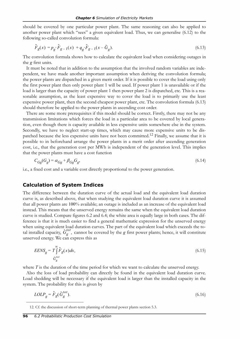
Chapter 6 Simulation of Electricity Markets
should be covered by one particular power plant. The same reasoning can also be applied toanother power plant which “sees” a given equivalent load. Thus, we can generalise (6.12) to thefollowing so-called convolution formula:
= pg· + qg· (6.13)
The convolution formula shows how to calculate the equivalent load when considering outages inthe g first units.
It must be noted that in addition to the assumption that the involved random variables are inde-pendent, we have made another important assumption when deriving the convolution formula;the power plants are dispatched in a given merit order. If it is possible to cover the load using onlythe first power plant then only power plant 1 will be used. If power plant 1 is unavailable or if theload is larger than the capacity of power plant 1 then power plant 2 is dispatched, etc. This is a rea-sonable assumption, as the least expensive way to cover the load is to primarily use the leastexpensive power plant, then the second cheapest power plant, etc. The convolution formula (6.13)should therefore be applied to the power plants in ascending cost order.
There are some more prerequisites if this model should be correct. Firstly, there may not be anytransmission limitations which forces the load in a particular area to be covered by local genera-tion, even though there is capacity available in less expensive units somewhere else in the system.Secondly, we have to neglect start-up times, which may cause more expensive units to be dis-patched because the less expensive units have not been committed.12 Finally, we assume that it ispossible to in beforehand arrange the power plants in a merit order after ascending generationcost, i.e., that the generation cost per MWh is independent of the generation level. This impliesthat the power plants must have a cost function
CGg(Gg) = αGg + βGgGg, (6.14)
i.e., a fixed cost and a variable cost directly proportional to the power generation.
Calculation of System Indices
The difference between the duration curve of the actual load and the equivalent load durationcurve is, as described above, that when studying the equivalent load duration curve it is assumedthat all power plants are 100% available; an outage is included as an increase of the equivalent loadinstead. This means that the unserved energy remains the same when the equivalent load durationcurve is studied. Compare figures 6.2 and 6.4; the white area is equally large in both cases. The dif-ference is that it is much easier to find a general mathematic expression for the unserved energywhen using equivalent load duration curves. The part of the equivalent load which exceeds the to-tal installed capacity, cannot be covered by the g first power plants; hence, it will constituteunserved energy. We can express this as
EENSg = (6.15)
where T is the duration of the time period for which we want to calculate the unserved energy.Also the loss of load probability can directly be found in the equivalent load duration curve.
Load shedding will be necessary if the equivalent load is larger than the installed capacity in thesystem. The probability for this is given by
LOLPg = (6.16)
12. Cf. the discussion of short-term planning of thermal power plants section 5.3.
Fg x( ) Fg 1– x( ) Fg 1– x Gg–( ).
Ggtot,
T Fg x( ) x,d
Ggtot
∞
∫
Fg Ggtot( ).
96 6.2 Probabilistic Production Cost Simulation

Chapter 6 Simulation of Electricity Markets
To be able to calculate the total operation cost it is necessary to know the expected generation ineach power plant. Unlike the unserved power the expected generation is however not unchangedwhen the equivalent load duration curve is calculated. This is clearly visible when comparing fig-ures 6.2 and 6.4; the shaded area is larger in the latter figure. The expected generation of a powerplant can however by determined by studying how the power plant affects the unserved energy inthe system. Before power plant g is added to the system we have the unserved energy EENSg – 1.After using (6.13) we get the unserved energy EENSg. he difference between these values must ofcourse be due to energy generation in power plant g; thus we can calculate the expected genera-tion by
EGg = EENSg – 1 – EENSg. (6.17)
An alternative way of calculating the expected generation is to use the following formula:13
EGg = (6.18)
Verification and derivation of this formula is left to the reader; see exercises 6.2 and 6.3.As we know the expected generation in each power plant it is possible to calculate the total oper-
ation cost by summation of the expected costs in each power plant:
(6.19)
where βGk is the variable operation cost in the cost function (6.14).Example 6.8. Calculate the unserved energy, loss of load probability and expectedoperation cost per hour in the system described in figure 6.3.Solution: The load duration curve is given in the figure:
The larger power plant has the lower operation cost and should therefore be addedfirst:
=
=
Then the second power plant is added:
=
13. It should be noted that this formula cannot be applied to power plants which have more than one possiblestate of availability (see section 6.2.4).
T pg Fg 1– x( ) x.d
Gg 1–tot
Ggtot
∫⋅
ETOCg βGkEGk,k 1=
g
∑=
F0 x( )1
0.20⎩
⎪⎨⎪⎧ x 200,<
200 x 300,<≤300 x≤ .
=
F1 x( ) 0.8F0 x( ) 0.2F0 x 200–( )+=
0.8 1 0.2 1⋅+⋅ 1=0.8 0,2 0.2 1⋅+⋅ 0.36=
0.8 0 0.2 1⋅+⋅ 0.2=0.8 0 0.2 0.2⋅+⋅ 0.04=
0⎩⎪⎪⎨⎪⎪⎧ x 200,<
200 x 300,<≤300 x 400,<≤400 x 500,<≤
500 x.≤
F2 x( ) 0.5F1 x( ) 0.5F1 x 100–( )+=
6.2 Probabilistic Production Cost Simulation 97

Chapter 6 Simulation of Electricity Markets
=
To calculate the expected generation in the two power plants we must know theunserved energy before and after adding the power plants to the equivalent load dura-tion curve. Since we want to calculate the operation cost per hour it is most practicalto use the same period length in the calculations of unserved energy and expectedgeneration:
EENS0 = = 1·200 + 0.2·100 = 220 kWh,
EENS1 = = 0.36·100 + 0.2·100 + 0.04·100 = 60 kWh,
EENS2 = = 0.28·100 + 0.12·100 + 0.02·100 = 42 kWh,
EG1 = EENS0 – EENS1 = 160 kWh,
EG2 = EENS1 – EENS2 = 18 kWh.
It is now easy to calculate the expected operation cost per hour:ETOC = β1·EG1 + β2·EG2 = 1·160 + 2·18 = 196 ¤/h.
The loss of load probability is given by
LOLP = = 28%
and the unserved energy is 42 kWh/h, as we already have calculated
6.2.2 Load ModelWhen using the method of probabilistic production cost simulation the load is described solely bya duration curve. This means that we either assumed that the producers are obliged to supply theload as long as it is technically possible or that the load is price independent (i.e., the consumersare willing to pay any price as long as their load is supplied). Obligation to supply is common inregulated electricity market, where it is common with so-called concession holders, which havemonopoly on power delivery within a specified area, but also are obliged to supply all consumerswithin that area. In modern restructured electricity markets there is a tendency that the consumersare becoming more price sensitive, but it is still a reasonable simplification to assume price inde-pendent load.
In those cases when the load is assumed to follow some given probability distribution, e.g. thenormal distribution, the load duration curve can easily be calculated using the definitions given inappendices C and D. Below we will show how the load duration curve can be determined startingfrom a specified typical load profile:
0.5 1 0.5 1⋅+⋅ 1=0.5 0.36 0.5 1⋅+⋅ 0.68=
0.5 0.2 0.5 0.36⋅+⋅ 0.28=0.5 0.04 0.5 0.2⋅+⋅ 0.12=0.5 0 0.5 0.04⋅+⋅ 0.02=
0⎩⎪⎪⎪⎨⎪⎪⎪⎧ x 200,<
200 x 300,<≤300 x 400,<≤400 x 500,<≤500 x 600,<≤
600 x.≤
1 F0 x( ) xd0
∞
∫⋅
1 F1 x( ) xd200
∞
∫⋅
1 F2 x( ) xd300
∞
∫⋅
F2 300( )
98 6.2 Probabilistic Production Cost Simulation

Chapter 6 Simulation of Electricity Markets
Definition 6.11. The load curve, D(k), states the mean load per hour during a spec-ified time period: k = 1, …, T.14
A given load curve can be transformed into the real load duration curve by sorting the load levelsin descending order. This means that the real load duration curve is defined as follows:
Definition 6.12. The real load duration curve, LDCR(k), states the load level whichis exceeded during k hours.
It should be noted that information is lost during the transformation from load curve to real loadduration curve, as it is no longer possible to determine how fast the load is increasing or decreas-ing, or how often a given load level will be exceeded during a given time period.
Example 6.9. Table 6.3 shows the load during a typical day in a system. Draw thereal load duration curve of this load.
Solution: In figure 6.5 the load curve corresponding to the values stated in table 6.3 isshown. The real load duration curve is obtained by simply sorting the load levels ofthe load curve in descending order, as shown in figure 6.6. The curve should be inter-preted so that the peak load 700 MWh/h is exceeded during 3 hours (and hence alsoduring 1 or 2 hours), etc.
The next step is to switch the axis of the real load duration curve:Definition 6.13. The inverted load duration curve, LDC(x), states how many hours
14. Some other period length than an hour can be used if desirable.
Table 6.3 Load during a typical day in example 6.9.
Hour Load [MWh/h] Hour Load [MWh/h] Hour Load [MWh/h]
1 400 9 700 17 7002 400 10 700 18 6003 500 11 600 19 6004 500 12 500 20 6005 500 13 500 21 5006 600 14 500 22 5007 600 15 600 23 5008 600 16 600 24 400
10 h
k
5 15
800
600
400
200
20
MWh/h D
10 h
k
5 15
800
600
400
200
20
MWh/h LDCR
Figure 6.5 Load curve of the load intable 6.3.
Figure 6.6 Real duration curve of theload in table 6.3.
6.2 Probabilistic Production Cost Simulation 99

Chapter 6 Simulation of Electricity Markets
a certain load level x is exceeded.The inverted load duration curve is valid for a specified time period. By normalising the verticalaxis, i.e., dividing all values by the duration of the studied time period, T, a normalised load dura-tion curve is obtained. This is the more formal term for what we in section 6.2.1 referred to as theload duration curve; however, we will continue to use the shorter term. The definition of a loadduration curve is completely in accordance to the general definition of duration curves which isgiven in appendix C.
Example 6.10. Determine the load duration curve of the load in example 6.9.Solution: Switching axis of the real load duration curve from figure 6.6 results in theinverted load duration curve shown in figure 6.7. The load duration curve is thenobtained by scaling the inverted load duration curve.Alternatively, the problem could have been solved using the data from table 6.3directly. The frequency function, i.e., the probability of a specified load level is easilycomputed from the table:
fD(x) =
Using theorem C.4 we get
which is exactly the same duration curve as shown in figure 6.8.In the examples above we have only considered simple loads which only have a few possible lev-
els. In reality the load is of course a continuous random variable. The earlier stated formu-
400 MWh/h
x
200 600
25
15
10
5
800
h LDC
20
400 MWh/h
x
200 600 800
FD
Figure 6.7 The inverted dura-tion curve of the loadin table 6.3.
Figure 6.8 Duration curve of theload in table 6.3.
1
0.6
0.8
0.4
0.2
3 24⁄ 0.125=9 24⁄ 0.375=9 24⁄ 0.375=3 24⁄ 0.125=⎩
⎪⎪⎨⎪⎪⎧ x 400,=
x 500,=x 600,=x 700.=
FD x( ) fD t( )t x>∑
0.125 0.375 0.375 0.125+ + + 1=0.375 0.375 0.125+ + 0.875=
0.375 0.125+ 0.5=0.125
0⎩⎪⎪⎨⎪⎪⎧
= =
x 400,<400 x 500,<≤500 x 600,<≤600 x 700,<≤
700 x,≤
100 6.2 Probabilistic Production Cost Simulation

Chapter 6 Simulation of Electricity Markets
lae—both concerning the load duration curve and calculation of system indices—are valid alsothen, but the calculations are harder. Therefore, it is appropriate to divide a continuous load dura-tion curve into constant segments, i.e., to approximate the continuous function by a staircase-looking function, similar to the one obtained in example 6.10. The segment size (in MWh/h) cor-respond to the width of the “steps”. For a given segment size it is then possible to represent theduration curve using a vector.
Example 6.11. What is the vector representation of the load duration curve inexample 6.10?Solution: In this case it is natural to use the step size 100 MWh/h, which means thatthe vector representation becomes [1 1 1 1 0.875 0.5 0.125 0]. The first element shouldbe interpreted as the value of in the first segment, i.e., 0 ≤ x < 100, the secondelement is the value in the second segment 100 ≤ x < 200, etc.
Given a specified segment size there are several possible ways to divide a continuous durationcurve into segments. It is appropriate to select a segmentation which does not change the area be-low the duration curve, since this area is related to the expectation value of the corresponding ran-dom variable (according to theorem C.10). Performing a segmentation according to this principlemay need quite a lot of work and is therefore not always worth the pains. Instead of putting a largeeffort on finding the best approximation it might be better to just reduce the segment size.
Example 6.12 (segmentation of a load duration curve): Suppose that theload in a system is normally distributed and has a mean value of 300 MW and a stand-ard deviation of 50 MW. Approximate the load duration curve using two segmentsizes: 50 MW and 100 MW respectively.Solution: First we have to select a method to determine the value in each segment ofthe approximated load duration curve A simple method is to assume that thecontinuous load duration curve is more or less linear within each segment, and thenchoose as the mean of the linear approximation:
for (s – 1) · Δx ≤ x < s · Δx,
where s denotes the s:th segment and Δx is the segment size. The result of applyingthis strategy is shown in figure 6.9. As can be seen in the figure, the assumption aboutlinearity is reasonable around the mean load 300 MW, but is less good for low and
FD x( )
400 MWh/h
x
200 600
FD
100 300 500 700
Figure 6.9 Approximation of the load duration curve inexample 6.12.
1
0.6
0.8
0.4
0.2
FD* .
FD*
FD* x( )FD s 1–( ) Δx⋅( ) FD s Δx⋅( )+
2------------------------------------------------------------------------=
6.2 Probabilistic Production Cost Simulation 101

Chapter 6 Simulation of Electricity Markets
high load levels. The error is significantly larger in the approximation using the widerstep length (dashed line in the figure).
6.2.3 Model of Thermal Power PlantsIn section 6.2.1 we used a power plant model where the units were characterised by three proper-ties: the installed capacity generation cost βG, and availability p. This model is suitable for ther-mal power plants.
The installed capacity of a power plant hardly offers any problem to determine, as it is definedby the technical performance of the equipment in the power plant. The operation cost of thermalpower plants have already been treated in section 5.3.2. Notice that a probabilistic production costsimulation cannot consider start-up or stop costs, as all information about the time-line of eventsis lost when a chronological load curve is transformed into a load duration curve (cf.section 6.2.2).
The availability is difficult to calculate using a theoretical model and must in practice be based onassumptions, for example by comparison to operational statistics of similar power plants. A powerplant can not be operated continuously; every now and then it has to be stopped for maintenance.We can distinguish between corrective and preventive maintenance. Corrective maintenancemeans that a vital component must be repaired in order to allow the power plant to generatepower. Corrective maintenance is thus performed after failures and can not be anticipated. Thepurpose of preventive maintenance is to reduce the risk of failures and is performed both for eco-nomical and security reasons. The preventive maintenance must be planned in advance, so that thepower plant is taken off-line at some occasion when the disturbance is as small as possible. TheSwedish nuclear power plants are for example maintained during the summer, when the load inthe Swedish system is low.
The convolution formula (6.13) is based on the assumption that load and outages in powerplants are independent random variables. This is a reasonable assumption for failures in powerplants. Preventive maintenance is however scheduled to specified occasions and there will there-fore be a correlation between the load and preventive maintenance. This problem can be avoided(for example by performing separate calculations of the system indices during those periods whenimportant power plants are stopped for maintenance), but to simplify the presentation we willrestrict ourselves to studying corrective maintenance in this compendium.
During the time the power plant is repaired it is said to be unavailable; the remaining time it isavailable. Notice that an available power plant is not necessarily dispatched, as the load might be solow that the power plant is not needed. The availability of a power plant is the probability of thepower plant being available. The most simple way to calculate the availability is to study statisticsof the operation of the power plant (or a similar power plant). These calculations require the fol-lowing notions:
Definition 6.14. The Mean Time To Failure is calculated by15
MTTF =
where K is the number of periods when the power plant is available and tu(k) is theduration of each of these periods.Definition 6.15. The Mean Time To Repair is calculated by16
15. This footnote has just been added to maintain the footnote numbering in pace with the Swedish edition.16. This footnote has just been added to maintain the footnote numbering in pace with the Swedish edition.
G,
1K---- tu k( ) ,
k 1=
K
∑
102 6.2 Probabilistic Production Cost Simulation
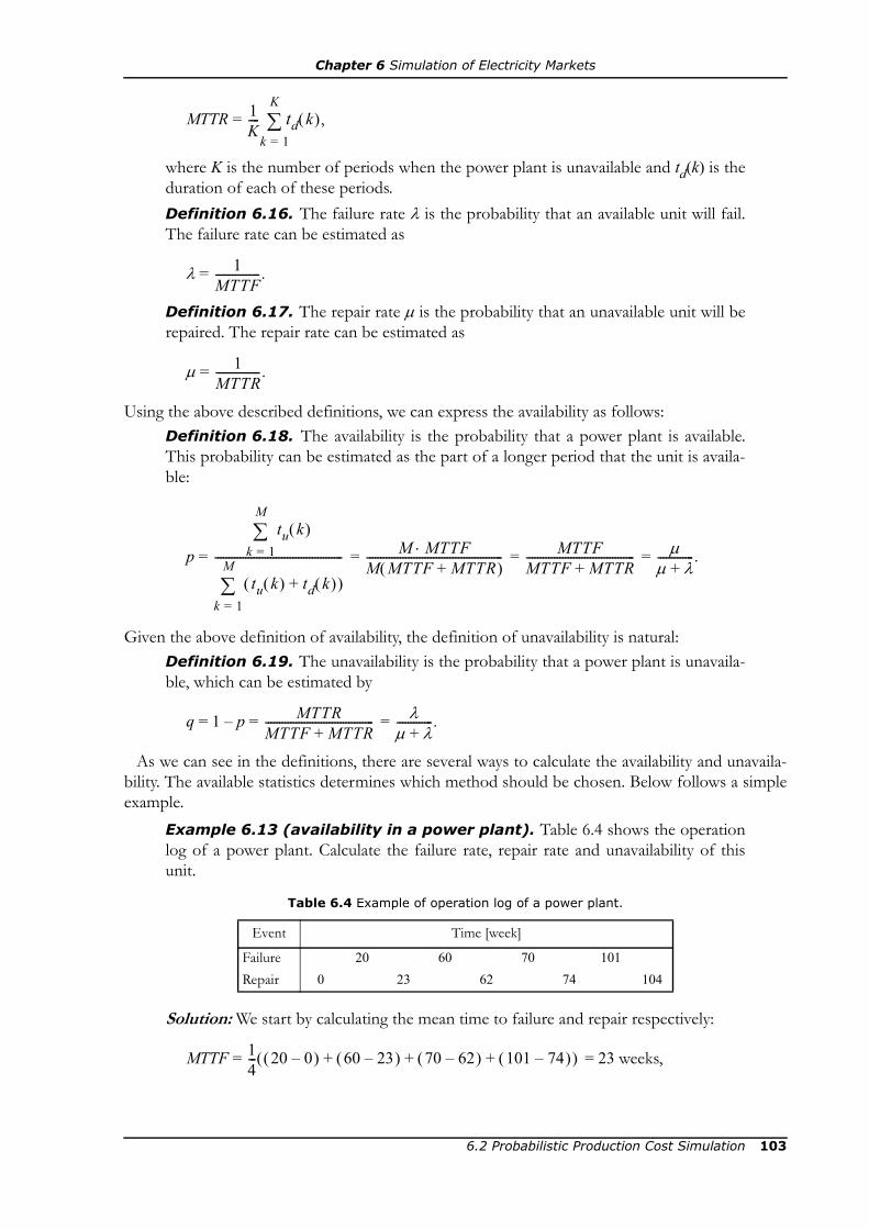
Chapter 6 Simulation of Electricity Markets
MTTR =
where K is the number of periods when the power plant is unavailable and td(k) is theduration of each of these periods.Definition 6.16. The failure rate λ is the probability that an available unit will fail.The failure rate can be estimated as
λ =
Definition 6.17. The repair rate μ is the probability that an unavailable unit will berepaired. The repair rate can be estimated as
μ =
Using the above described definitions, we can express the availability as follows:Definition 6.18. The availability is the probability that a power plant is available.This probability can be estimated as the part of a longer period that the unit is availa-ble:
p = = = =
Given the above definition of availability, the definition of unavailability is natural:Definition 6.19. The unavailability is the probability that a power plant is unavaila-ble, which can be estimated by
q = 1 – p = =
As we can see in the definitions, there are several ways to calculate the availability and unavaila-bility. The available statistics determines which method should be chosen. Below follows a simpleexample.
Example 6.13 (availability in a power plant). Table 6.4 shows the operationlog of a power plant. Calculate the failure rate, repair rate and unavailability of thisunit.
Solution: We start by calculating the mean time to failure and repair respectively:
MTTF = = 23 weeks,
Table 6.4 Example of operation log of a power plant.
Event Time [week]
Failure 20 60 70 101Repair 0 23 62 74 104
1K---- td k( ),
k 1=
K
∑
1MTTF---------------- .
1MTTR---------------- .
tu k( )k 1=
M
∑
tu k( ) td k( )+( )k 1=
M
∑---------------------------------------------- M MTTF⋅
M MTTF MTTR+( )------------------------------------------------- MTTF
MTTF MTTR+--------------------------------------- μ
μ λ+------------- .
MTTRMTTF MTTR+--------------------------------------- λ
μ λ+------------- .
14--- 20 0–( ) 60 23–( ) 70 62–( ) 101 74–( )+ + +( )
6.2 Probabilistic Production Cost Simulation 103

Chapter 6 Simulation of Electricity Markets
MTTR = = 3 weeks.
The failure and repair rates can now be calculated according to their definitions:
λ = ≈ 0.0435 failures/week (when the power plant is available),
μ = ≈ 0.3333 repairs/week (when the power plant is unavailable).
When calculating the unavailable we assume that the two years recorded in the opera-tion log are representative; hence, the unavailability is estimated to
q = = ≈ 0.1154.
6.2.4 Wind Power ModelA wind power plant converts the kinetic energy of the wind into electric energy. Since the windspeed is varying so will the electricity generation. Figure 6.10 shows the electricity generation as afunction of the wind speed for two different types of wind power plants. The turbine in the left di-agram is pitch controlled, which means that when the wind speed is higher than vr the wind is“spilled” by feathering the blades. The motive for this solution is that it is not necessary to dimen-sion important parts (as for example the gearbox and the generator) for power levels that arerather rare. The optimal level of rated power in this type of power plant is thus a trade-off betweenthe costs of designing the power plant for high wind speeds and the income of the energy sales.The wind power plant in the right diagram is stall regulated, which have a fixed blade angle. How-ever, at high wind speeds, some of the wind passes by due to turbulence. An advantage of this typeof turbine compared to the pitch controlled units is that there is no need to invest in controlequipment. A minor disadvantage is that the peak capacity is not exactly defined and the peak isonly obtained for a relatively small wind speed interval. Both types of units are shut down at highwind speeds, because the wind gets too turbulent then, which causes unacceptable strains on theunit.
14--- 23 20–( ) 62 60–( ) 74 70–( ) 104 101–( )+ + +( )
1MTTF----------------
1MTTR----------------
MTTRMTTF MTTR+--------------------------------------- 3
3 23+---------------
10 m/s
v
kW W(v)
5 15
2 000
1 500
1 000
500
20 25 10 m/s
v
5 15
2 000
1 500
1 000
500
20 25
kW W(v)
Figure 6.10 The relation between wind speed and electricity generation for two kindsof wind power plants (Vestas V80-2.0 MW and NEG Micon NM 1500C).
vr
104 6.2 Probabilistic Production Cost Simulation

Chapter 6 Simulation of Electricity Markets
Available Generation Capacity
The electricity generation in a wind power plant is depending on whether the plant is technicallyavailable or not, as well as the current wind speed. To obtain a density function of the availablegeneration capacity of a wind power plant it is therefore necessary to include both the availabilityof the unit and the wind speed distribution.
If actual wind speed statistics for a site is available then these statistics should of course be usedas basis for the wind power model. However, if such statistics are not available then it is commonto assume that the wind is Rayleigh distributed. This means that the wind speed has the followingduration curve:
(6.20)
where α is a scaling parameter. Figure 6.11 shows examples of the density function and durationcurve of Rayleigh distributed wind speeds with the mean wind speed 5 m/s and 10 m/s respec-tively. As can be seen, the Rayleigh distribution resembles the normal distribution; the main differ-ence is that a Rayleigh distributed random variable never can obtain negative values. The relationbetween α and the mean wind speed can be calculated using theorem C.10:
μv = ≈ 0.89α. (6.21)
Let us now study the probability that the available wind power generation capacity in a 100%reliable wind power plant is larger than W kW. If v(W) is the inverse function of the electricitygeneration as function of the wind speed, W, and vco is the wind speed for which the wind powerplant is disconnected, then the wanted probability is equal to the probability that the wind speedbelongs to the interval [v(W), vco], i.e.,
(6.22)
It is of course only possible to apply (6.22) when the function v(W) exists. This is the case for pitchcontrolled wind power plants, where v(W) is the inverse function of W(v) in the interval v ∈ (0, vr).
Fv v( )1 v 0,<
e v α⁄( )2– v 0,≥⎩⎨⎧
=
10 m/s
v
5 15 20 25
FV
10 m/s
v
5 15 20 25
fV
0.2
0.1
0.05
0.15
Figure 6.11 The density function and duration curves of Rayleigh distributedwind speeds.
μv = 5 m/s
μv = 5 m/s
μv = 10 m/s μv = 10 m/s
1
0.6
0.8
0.4
0.2
0 Fv˜ v( ) vd
0
∞
∫+ e v α⁄( )2– vd0
∞
∫12---α π= =
FW W( ) Fv v W( )( ) Fv vco( )– ev W( )( )
α-----------------⎝ ⎠
⎛ ⎞ 2–
evcoα
-------⎝ ⎠⎛ ⎞
2–
.–= =
6.2 Probabilistic Production Cost Simulation 105

Chapter 6 Simulation of Electricity Markets
For stall regulated units there is no inverse function of W(v) in that interval (cf. figure 6.10). In or-der to model stall regulated wind power plants it is necessary to approximate the generation func-tion W(v) by a non-decreasing function.
There will be a strong correlation between the generation in wind power units whenever severalunits are located in the same area, since the wind speed will be more or less the same for allunits.17 To fulfil the requirement that all random variables in a probabilistic production cost simu-lation should be independent it is simplest to create a single model for the total generation of thewind farm. In this model we will also consider that the turbines are not 100% available. In order tosimplify the calculations, we will neglect the variations of the wind speed and assume that all tur-bines of the wind farm have exactly the same generation function W(v) and availability p. The totalwind power generation is then only depending on the current wind speed and the number of avail-able wind power plants.
The density function of the total wind power generation, Wtot, is quite obvious when all turbinesare unavailable:
(6.23)
If exactly n turbines are available (n > 0) then the probability that the total wind power generationequals Wtot is equal to the probability that each of the available turbines is generating Wtot/n, as weassume that the wind speed is the same for all units and all units are generating the same power fora given wind speed. Thus, we get the following probability density function:
n > 0, (6.24)
where is given by (6.22).To consider that the number of available turbines also is a random variable we can summarise
the density functions according to (6.23) and (6.24), while weighting each density function by theprobability of having exactly n units available. The result is the following probability density for awind farm of N power plants:
(6.25)
where
p = availability of a single unit,q = unavailability of a single unit = 1 – p,
= binomial coefficient, i.e, the number of ways to select n elements from a total population of N elements
It should be noted that Wtot according to (6.25) is a continuous random variable. Those are, as al-ready have been mentioned in section 6.2.2, impractical to use when performing probabilistic pro-duction cost simulations; therefore, it is appropriate to divide these density functions into seg-ments too. It is recommended to use the same segment size as for the segmentation of the loadduration curve.
Example 6.14 (model of a small wind farm): Assume that there is a windfarm with two identical units. From the wind conditions at the site the following
17. Small variations will be caused by the topology of the site. Moreover, windward units will “steal” somewind from leeward units.
fWtot
0 1 Wtot 0,=
0 Wtot 0.≠⎩⎨⎧
=
fWtot
n Wtot( ) fWWtot
n----------⎝ ⎠
⎛ ⎞ ddWtot--------------FW
Wtotn
----------⎝ ⎠⎛ ⎞ ,–= =
FW
fWtotWtot( ) pnq N n–( ) N
n⎝ ⎠⎛ ⎞ fWtot
n Wtot( ),n 0=
N
∑=
Nn⎝ ⎠
⎛ ⎞
106 6.2 Probabilistic Production Cost Simulation

Chapter 6 Simulation of Electricity Markets
model of the individual plants has been obtained (excluding the probability of fail-ures):
fW(W) =
Determine a model of the total power generation in the wind farm if the availability ofthe units are 99%.Solution: If none of the units is available then we get the trivial frequency function
= 1 when Wtot equals zero; otherwise we have = 0. If one of the units isavailable then = fW(Wtot), and when both units are available the result is
= fW(Wtot/2), i.e.,
=
The probability that none of the units is available is 0,01·0,01 = 10–4. The probabilitythat the first unit is available but not the second is 0,99·0,01 = 0,0099, which is as prob-able as the second unit being available but not the first. Hence, the probability thatone unit is available is 2·0,0099 = 0,0198. Finally, the probability of both units beingavailable is 0,99·0,99 = 0,9801. The frequency function of the total generation is then
= =
=
Calculation of System Indices for Wind Power Systems
The convolution formula (6.13) is based on the assumption that a power plant either is generatingits installed capacity or nothing at all. Moreover, it is assumed that load variations and failures inpower plants are independent, i.e., failures are equally likely for all load levels. These assumptionsare however not correct for wind power.
The wind power generation can, as described above, take any value between zero and installedcapacity. Each of these levels have a given probability which is stated by the probability densityfW(x). To calculate the equivalent load duration curve we can generalise (6.13) to the followingequation:
(6.26)
where
Ng = number of states in power plant g,pg, i = = probability of state i,
0.2 W 0,=0.4 W 300,=0.4 W 600.=⎩
⎪⎨⎪⎧
fWtot0 fWtot
0
fWtot1 Wtot( )
fWtot2 Wtot( )
fWtot2 Wtot( )
0.2 Wtot 0,=
0.4 Wtot 600,=
0.4 Wtot 1 200.=⎩⎪⎨⎪⎧
fWtotWtot( ) 0.0001fWtot
0 Wtot( ) 0.0198fWtot1 Wtot( ) 0.9801fWtot
2 Wtot( )+ +
0.0001 1 0.0198 0.2 0.9801 0.2⋅+⋅+⋅ 0.20008=
0.0001 0 0.0198 0.4 0.9801 0⋅+⋅+⋅ 0.00792=
0.0001 0 0.0198 0.4 0.9801 0.4⋅+⋅+⋅ 0.39996=
0.0001 0 0.0198 0 0.9801 0.4⋅+⋅+⋅ 0.39204=⎩⎪⎪⎨⎪⎪⎧ Wtot 0,=
Wtot 300,=
Wtot 600,=
Wtot 1 200.=
Fg x( ) pg i, Fg 1– x xg i,–( ),i 1=
Ng
∑=
fWg W xg i,–( )
6.2 Probabilistic Production Cost Simulation 107
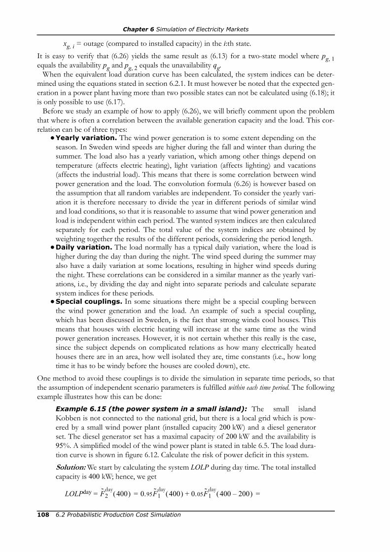
Chapter 6 Simulation of Electricity Markets
xg, i = outage (compared to installed capacity) in the i:th state.It is easy to verify that (6.26) yields the same result as (6.13) for a two-state model where pg, 1equals the availability pg and pg, 2 equals the unavailability qg.
When the equivalent load duration curve has been calculated, the system indices can be deter-mined using the equations stated in section 6.2.1. It must however be noted that the expected gen-eration in a power plant having more than two possible states can not be calculated using (6.18); itis only possible to use (6.17).
Before we study an example of how to apply (6.26), we will briefly comment upon the problemthat where is often a correlation between the available generation capacity and the load. This cor-relation can be of three types:
•Yearly variation. The wind power generation is to some extent depending on theseason. In Sweden wind speeds are higher during the fall and winter than during thesummer. The load also has a yearly variation, which among other things depend ontemperature (affects electric heating), light variation (affects lighting) and vacations(affects the industrial load). This means that there is some correlation between windpower generation and the load. The convolution formula (6.26) is however based onthe assumption that all random variables are independent. To consider the yearly vari-ation it is therefore necessary to divide the year in different periods of similar windand load conditions, so that it is reasonable to assume that wind power generation andload is independent within each period. The wanted system indices are then calculatedseparately for each period. The total value of the system indices are obtained byweighting together the results of the different periods, considering the period length.
•Daily variation. The load normally has a typical daily variation, where the load ishigher during the day than during the night. The wind speed during the summer mayalso have a daily variation at some locations, resulting in higher wind speeds duringthe night. These correlations can be considered in a similar manner as the yearly vari-ations, i.e., by dividing the day and night into separate periods and calculate separatesystem indices for these periods.
•Special couplings. In some situations there might be a special coupling betweenthe wind power generation and the load. An example of such a special coupling,which has been discussed in Sweden, is the fact that strong winds cool houses. Thismeans that houses with electric heating will increase at the same time as the windpower generation increases. However, it is not certain whether this really is the case,since the subject depends on complicated relations as how many electrically heatedhouses there are in an area, how well isolated they are, time constants (i.e., how longtime it has to be windy before the houses are cooled down), etc.
One method to avoid these couplings is to divide the simulation in separate time periods, so thatthe assumption of independent scenario parameters is fulfilled within each time period. The followingexample illustrates how this can be done:
Example 6.15 (the power system in a small island): The small islandKobben is not connected to the national grid, but there is a local grid which is pow-ered by a small wind power plant (installed capacity 200 kW) and a diesel generatorset. The diesel generator set has a maximal capacity of 200 kW and the availability is95%. A simplified model of the wind power plant is stated in table 6.5. The load dura-tion curve is shown in figure 6.12. Calculate the risk of power deficit in this system.Solution: We start by calculating the system LOLP during day time. The total installedcapacity is 400 kW; hence, we get
LOLPday = = =F2day
400( ) 0.95F1day
400( ) 0.05F1day
400 200–( )+
108 6.2 Probabilistic Production Cost Simulation

Chapter 6 Simulation of Electricity Markets
= +
+ == 0.95·(0.3 · 0 + 0.4 · 0 + 0.3 · 0.1) + 0.05·(0.3 · 0.1 + 0.4 · 0.7 + 0.3 · 1) = 5.9%.
In the same way we can calculate the night time LOLP:
LOLPnight = 0.95·(0.1 · 0 + 0.5 · 0 + 0.4 · 0) + + 0.05·(0.1 · 0 + 0.5 · 0.2 + 0.4 · 1) = 2.5%.
To calculate the total system LOLP we use the weighted average of these two values:
LOLP = ≈ 4.5%.
6.2.5 Model of Dispatchable Hydro PowerHydro power plants can be divided into two types: run-of-the-river plants and dispatchable plants.A run-of-the-river plant has no reservoir, which means that the available generation capacity is de-termined by whether or not the power plant is technically available, and the water flow at the siteof the plant. Thus, a run-of-the-river plant has similar properties as a wind power plant and can beincluded in a probabilistic production cost simulation using models resembling those described insection 6.2.4.
Dispatchable hydro power, i.e., hydro power plants having reservoirs, are not as dependent ofthe river flow, since water from the reservoir can be used when the natural flow is low. It is ratherthe available energy (i.e., the size of the inflow to the reservoirs during a year or some other appro-
100 kW
x
50 150 200 250
FDday
100 kW
x
50 150 200 250
FDnight
a) Day time (7 a.m. to 9 p.m.) b) Night time (9 p.m. to 7 a.m.).
Figure 6.12 The load for the small island in example 6.15.
1
0.6
0.8
0.4
0.2
1
0.6
0.8
0.4
0.2
Table 6.5 Model of the wind power plant in example 6.15.
Outage [kW]
Probability during the day
[%]
Probability during the night
[%]
0 30 10100 40 50200 30 40
0.95 0.3FDday
400 0–( ) 0.4FDday
400 100–( ) 0.3FDday
400 200–( )+ +( )⋅
0.05 0.3FDday
200 0–( ) 0.4FDday
200 100–( ) 0.3FDday
200 200–( )+ +( )⋅
1424------LOLPday 10
24------LOLPnight+
6.2 Probabilistic Production Cost Simulation 109

Chapter 6 Simulation of Electricity Markets
priate time period) which limits the electricity generation in these plants. As hydro power plants ingeneral have negligible or very small operation costs, the best way to utilise the available dispatch-able hydro energy is to replace the generation in the most expensive thermal power plants. In thissection we will describe a simple method to approximately determine which thermal power plantshould be replaced given a particular energy limit of the dispatchable hydro power.
The Impact of Hydro Power on Operation Costs
The operation cost of a hydro power plant is generally smaller than the operation cost of thermalpower plants. Therefore, it is obvious that in a hydro-thermal power system the total operationcost, ETOC, will be reduced the more hydro energy which is available during the studied period.What the need is a method to determine the total operation cost as a function of the available hy-dro energy, i.e., ETOC(WH).
Probabilistic production cost is as described earlier based on the assumption that the powerplants are dispatched in a given merit order, which means that the g:th unit only is used when theequivalent load can not be covered by power plants 1, …, g – 1. The power plant which is first inthe merit order will be generating as much as possible. If the first and second unit are switchedthen the former first power plant will decrease its generation, since a part of the load will be cov-ered by the former second power plant instead. In other words, the expected generation of apower plant will decrease whenever the power plant is moved down in the merit order. This ena-bles us to calculate the total operation cost for at least some levels of the expected energy genera-tion in the hydro power. If a system has G thermal power plants and one dispatchable hydropower plant then we must perform G + 1 separate simulations in order to try all positions of thehydro power, which undeniably would require quite a lot of calculations. Fortunately, there is ashort cut.
Assume that we are given a merit order and then shifts power plant g and power plant g + 1.This will apparently not affect the expected energy generation of those power plants which aredispatched before the g:th unit, i.e., power plant 1, …, g – 1, because these power plants will seeexactly the same equivalent load as before; the equivalent load is as we know equal to the real loadplus outages in higher prioritised units. It is less obvious that the expected energy generation ofthe power plants positioned later than unit g + 1 in the merit order are not affected neither!
Theorem 6.20. Assume that there are two power plants having the installed capaci-ties and respectively, and the availability pA and pB respectively. Further,assume that these power plants are used to cover the equivalent load he sameequivalent load duration curve (i.e., will then be obtained, regardless of inwhich order the units are dispatched.Proof: We try to add unit A first:
=
=
Then we try to add unit B first:
=
GA GBFg.
Fg 2+ ),
Fg 1+AB
x( ) pAFg x( ) qAFg x GA–( ),+=
Fg 2+AB
x( ) pBFg 1+AB
x( ) qBFg 1+AB
x GB–( )+=
pB pAFg x( ) qAFg x GA–( )+( ) qB pAFg x GB–( ) qAFg x GA– GB–( )+( ).+
Fg 1+BA
x( ) pBFg x( ) qBFg x GB–( ),+=
Fg 2+BA
x( ) pAFg 1+BA
x( ) qAFg 1+BA
x GA–( )+=
110 6.2 Probabilistic Production Cost Simulation

Chapter 6 Simulation of Electricity Markets
=
The result is clearly that Since the expected generation only is affected in the two power plants which are switched, therewill only be two possible levels of the expected generation of the thermal power plants; one level ifthe power plant is dispatched before the hydro power and another—lower—level if the thermalpower plant is dispatched after the hydro power. Thus, by performing two simulations, one havingthe hydro power as the first power plant in the merit order and one there it is last in the merit or-der, it will be possible to calculate both levels of the expected generation in all thermal powerplants. With that, the expected generation of all thermal power plants can be calculated given aparticular priority for the hydro power. Knowing the expected generation it is also possible to cal-culate theETOC using (6.19). The result is a few points of the function ETOC(WH); or the remain-ing values of WH the ETOC can be determined using linear interpolation between the two closesknown points.
Example 6.16 (simulation of dispatchable hydro): The power plants in acertain electricity market are listed in table 6.6. The hydro power plant is dispatchableand the annual inflow is 1 TWh. The load duration curve is shown in figure 6.13.Determine the expected operation cost of the system.Solution: The simulations are performed according to the equations derived insection 6.2.1. The calculations need no special considerations, but are comparativelyspace consuming and are therefore excluded. The result of four simulations are shownin table 6.6. Actually, it would have been sufficient to simulate the system with themerit orders H, A, B, C and A, B, C, H respectively; the other two positions were onlysimulated to illustrate the claim that the expected generation in the thermal powerplants only has two possible levels, depending on whether the unit is dispatchedbefore or after the hydro power. We can also notice that the EENS and LOLP is notaffected by the merit order of the power plants.Using the results from table 6.6 it is possible to estimate the operation cost as a func-tion of the available hydro energy, as shown in figure 6.14. Using linear interpolationwe obtain ETOC ≈ 351,82 M¤/year in this case.
pA pBFg x( ) qBFg x GB–( )+( ) qA pBFg x GA–( ) qBFg x GB– GA–( )+( ).+
Fg 2+ x( ) Fg 2+AB
x( ) Fg 2+BA
x( ).= =
200 GWh/yearEGH
500
400
300
M¤/year ETOC
400 600 800 1 000 1 200 1 400 1 600 1 800 2 000
Figure 6.14 Estimation of the total operation cost in a system with dispatcha-ble hydro power as function of the available hydro energy. Thepoints obtained from the simulations are marked by small cir-cles. Between these points it is assumed that the function ispiecewise linear.
6.2 Probabilistic Production Cost Simulation 111

Chapter 6 Simulation of Electricity Markets
The Water Value
The water stored in the reservoirs has a value, as it can be used to replace future generation inmore expensive power plants. The marginal water value (often referred to just as the water value)is the decrease in the total operation cost given an extra MWh of available hydro energy. The unitof water value is therefore ¤/MWh. When considering the function ETOC(WH) the water value iscorresponding to the slope of the linear segments, which means that we will get different watervalues depending on the amount of available hydro energy. The explanation is that the dispatcha-ble hydro generation will be used to replace the most expensive thermal power plant. When theexpected generation of that plant is decreased to zero, then the hydro power will replace the sec-ond most expensive thermal power plant, etc. As the water value is equal to the operation cost ofthe last replaced thermal power plant it will be highest when there is just so much water availablethat a part of the energy generation in the most expensive thermal power plant can be replaced.
6.2.6 Simplified Calculation of the Loss of Load Probability
As shown in the earlier parts of section 6.2 it is necessary to perform quite a lot of calculationsduring probabilistic production cost simulations. The large amount of calculations is primarily dueto the convolution equations. For a real system with a large number of power plants of different
Table 6.6 Results of the simulations in example 6.16.
System indexMerit order
H, A, B, C A, H, B, C A, B, H, C A, B, C, H
EGA [GWh/year] 2 373.08 3 153.60 3 153.60 3 153.60
EGB [GWh/year] 224.10 224.10 946.08 946.08
EGC [GWh/year] 37.24 37.24 37.24 222.61
EGH [GWh/year] 1 734.48 953.96 231.99 46.61
ETOC [M¤/year] 278.37 356.42 464.72 501.79
EENS [GWh/year] 11.09 11.09 11.09 11.09
LOLP [%] 0.9 0.9 0.9 0.9
400 MWh/h
x
200 600
FD
Figure 6.13 Load duration curvein example 6.16.
Table 6.6 Power plants in example 6.16.
Power plant Capacity [MW]
Availa-bility [%]
Operation cost
[¤/MWh]
Dispatchable hydro H 200 99 0Thermal plant A 400 90 100Thermal plant B 300 90 150Thermal plant C 200 95 200
1
0.5
0.75
0.25
112 6.2 Probabilistic Production Cost Simulation

Chapter 6 Simulation of Electricity Markets
sizes and using a relatively large accuracy in the segmentation of the load duration curve (i.e., asmall segment size), the number of calculations become very large. In this section we will presenta faster, simplified method, which can be used to estimate the LOLP.
As mentioned in section 6.2.2 the load is often modelled by one or more normal distributions. Ifthat is not the case and a typical load profile is used instead, it is still possible to obtain a normalapproximation of the load:
μD = E[D], (6.27a)
σD = (6.27b)
i.e., it is assumed that the load is normally distributed and having the same expectation value andstandard deviation as the real load. The difference will hence be that the real load is likely to haveanother probability distribution. The expectation value and standard deviation can be calculatedusing the definitions and theorems stated in appendix C.
Example 6.17 (normal approximation of a load): Determine a normal ap-proximation of the load in examples 6.9 and 6.10.Solution: Since the frequency function of the load is known (from the solution toexample 6.10), we can directly apply definitions C.6 and C.7:
μD = 400·0.125 + 500·0.375 + 600·0.375 + 700·0.125 =
= 550 MW,
σD = =
= ≈≈ 86.6 MW.
Outages in power plants can also be considered to be approximately normally distributed. For atwo-state model we get
= E[Og] = pg·0 + qg· = qg· (6.28a)
= =
= = {pg = 1 – qg} =
= = { = qg· } = =
= = (6.28b)
For power plants having more than two possible states it is in most cases best to directly apply thedefinitions of expectation value and standard deviation.
Example 6.18 (normal approximation of a wind farm): Determine a nor-mal approximation of the wind farm from example 6.14Solution: The probability of having a given capacity available in the wind farm hasalready been calculated in example 6.14. The probability of an outage x = 1 200 – Wtotis
Var D[ ],
xfD x( )x∑=
x μD–( )2fD x( )x∑
150–( )2 0.125⋅ 50–( )2 0.375⋅ 502 0.375⋅ 1502 0.125⋅+ + +
μOgGg Gg,
σOgVar Og[ ] E Og μOg
–( )2[ ] pg 0 μOg–( )2 qg Gg μOg
–( )2+= =
pgμOg2 qgGg
2 2qgμOgGg– qgμOg
2++
μOg2 qgGg
2 2μOgqgGg–+ μOg
Gg qgGg2 qgGg( )2–
Gg qg qg2– Gg qgpg.
6.2 Probabilistic Production Cost Simulation 113

Chapter 6 Simulation of Electricity Markets
According to definitions C.6 and C.7 we get
= 0.39204·0 + 0.39996·600 + 0.00792·900 + 0.20008·1 200 =
= 487.2 kW,
= … ≈ 315.7 kW.
The basis of the convolution equation (6.13) and its generalised variant (6.26) is that the equiva-lent load is the sum of the actual load and outages in power plants. When both load and outagesare modelled by normal distributions it becomes possible to replace the convolution by summaris-ing normal distributions, which means that the equivalent load duration curve of g power plantscan—according to theorem D.4—be written as
∈ N(μg, σg) (6.29)
where
μg = (6.29a)
σg = (6.29b)
A power deficit occurs when the equivalent load exceeds the installed capacity. The probabilityof this is determined by
LOLPg ≈ (6.30)
It is important to remember that this approximation of the loss of load probability is based on theassumption that the equivalent load is at least approximately normally distributed. This is a reason-able assumption for large systems with approximately normally distributed load and power plantsof similar size.
Example 6.19. Assume that the load in example 6.17 should be covered by Gpower plants of 200 MW each. The availability of each plant is 80%. Calculate the riskof power deficit for G = 1, …, 12.Solution: he normal approximation of a single power plant can be obtained using(6.28a) and (6.28b):
= 0.2 · 200 = 40 MW,
= = 80 MW.
fOvx( )
0.39204
0.39996
0.00792
0.20008⎩⎪⎪⎨⎪⎪⎧
=
x 0,=x 600,=x 900,=
x 1 200.=
μOvxfOv
x( )x∑=
σOvx μOv
–( )2 fOvx( )( )
x∑=
FgN
μD μOg,
i 1=
g
∑+
σD2 σOg
2
i 1=
g
∑+ .
FgN
Ggtot( ) 1 Φ
Ggtot μg–
σg----------------------
⎝ ⎠⎜ ⎟⎛ ⎞
.–=
μOg
σOg200 0.2 0.8⋅
114 6.2 Probabilistic Production Cost Simulation

Chapter 6 Simulation of Electricity Markets
We can now apply (6.30). The results are listed in table 6.7. For comparison, theresults of the “exact” simulation18 using the equations (6.13) and (6.16) are alsoshown.Apparently it is possible to obtain results with rather large relative errors in the esti-mation of the LOLP using the simplified method, but the size of order is still correct.
6.3 MONTE CARLO SIMULATIONIt is not always possible to directly calculate expectation values according to their definition (whichis found inappendix C). The problem can either be that the integral itself is hard to solve or thatthe integrand is not known, for example because the density function of the random variable isunknown. An alternative for these cases is to use so-called Monte Carlo methods, which are basedon estimation of the properties of the variable by random observations. In section 6.1 we showedthat the system indices to be calculated in an electricity market simulation actually are the expecta-tion values of various result variables. Hence, Monte Carlo methods seem suitable for estimatingdifferent system indices.
In this section we will describe basic methods which can be used for Monte Carlo simulation ofelectricity markets. These methods are applied on fairly simple examples.
6.3.1 Simple SamplingBy simple sampling we refer to a sample survey, where we completely randomly select observa-tions—samples—of a random variable. From these samples it is possible to obtain an estimate ofthe probability distribution of the random variable.
Table 6.7 The risk of power deficit in example 6.19.
Number of power plants
LOLP
Using the simplified method
Using the exact method
1 0.9995 12 0.9468 0.9200
3 0.6658 0.5040
4 0.3104 0.2128
5 0.1042 0.0771
6 0.0278 0.0253
7 6.3435·10–3 7.7184·10–3
8 1.2933·10–3 2.2349·10–3
9 2.4316·10–4 6.2106·10–4
10 4.3046·10–5 1.6701·10–5
11 7.2789·10–6 4.3725·10–6
12 1.1878·10–6 1.1194·10–6
18. Remember that the earlier described method also is based on simplifications and assumptions.
6.3 Monte Carlo Simulation 115

Chapter 6 Simulation of Electricity Markets
Theory
The basic idea of all Monte Carlo methods is that the expectation value of a random variable canbe estimated by random observations of the variable. The expectation value can be interpreted asthe mean of an infinite series of observation of the random variable.19 It is—for natural rea-sons—impossible to perform an infinite series of experiments to determine the expectation value.However, the more observations that are made of a random variable, the more likely it will be thatthe mean of these observations is close to the expectation value. The expectation value can thusbe estimated by calculating the mean of a large enough number of observations. This is referred toas simple sampling.
Theorem 6.21. If there are n independent observations, x1, …, xn, of the randomvariable X then the mean of these observations, i.e.,
is an estimate of E[X].There is of course a formal proof of this theorem, but we will restrict ourselves to illustrating theprinciple in a simple example:
Example 6.20 (tossing a coin): Calculate the density function of the mean out-come when a coin is tossed 1, 2, 3, 10, 100 and 1 000 times respectively. Comparethese density function to the expectation value of the coin toss.Solution: Let the random variable C be equal to 0 if the result of tossing the coin wastails and 1 if it was heads. Introduce the symbol Hn for the mean of n coin tosses, i.e.,
Hn =
Notice that Hn is also a random variable, as it is a function of the sum of a number ofrandom observations.f the coin is tossed n times then it is possible to obtain 2n different outcomes, pro-vided that we take into account in which order the results were received. In this casethe order does not matter, as it is only the total number of heads that affect the mean.It is therefore sufficient to know how many of the 2n outcomes correspond to a givenvalue of Hn.Let h be the number of heads in a series of observations. The number of ways toselect h elements out of a population of n elements is given by the binomial coefficient
For n = 1 we get the binomial coefficients
= 1, = 1.
The interpretation is that when one experiment is performed then there is only oneway to have the outcome heads 0 times and 1 time respectively. For n = 2 we get
19. Cf. definition C.6.
mX1n--- xi
i 1=
n
∑=
1n--- ci
i 1=
n
∑ .
nh⎝ ⎠
⎛ ⎞ n!h! n h–( )!------------------------ .=
10⎝ ⎠
⎛ ⎞ 11⎝ ⎠
⎛ ⎞
116 6.3 Monte Carlo Simulation

Chapter 6 Simulation of Electricity Markets
0.2 10.80.60.4
x0.1
0.2
0.3
0.4
0.5
fH1
a) Density function after one trial. b) Density function after two trials.
Figure 6.15 Density function for the mean result tossing a coin.
c) Density function after three trials. d) Density function after ten trials.
e) Density function after 100 trials. f) Density function after 1 000 trials.
0.2 10.80.60.4
x
0.1
0.2
0.3
0.4
fH3
0.2 10.80.60.4
x0.05
0.1
0.15
0.2
0.25
fH10
0.2 10.80.60.4
x
0.02
0.04
0.06
0.08
fH100
0.2 10.80.60.4
x0.005
0.01
0.015
0.02
0.025
fH1000
0.2 10.80.60.4
x0.1
0.2
0.3
0.4
0.5
fH2
6.3 Monte Carlo Simulation 117
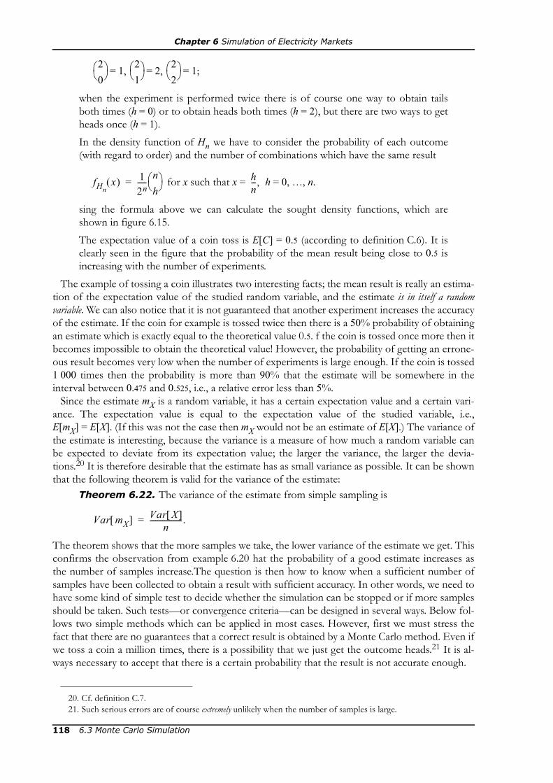
Chapter 6 Simulation of Electricity Markets
= 1, = 2, = 1;
when the experiment is performed twice there is of course one way to obtain tailsboth times (h = 0) or to obtain heads both times (h = 2), but there are two ways to getheads once (h = 1).In the density function of Hn we have to consider the probability of each outcome(with regard to order) and the number of combinations which have the same result
for x such that x = h = 0, …, n.
sing the formula above we can calculate the sought density functions, which areshown in figure 6.15.The expectation value of a coin toss is E[C] = 0.5 (according to definition C.6). It isclearly seen in the figure that the probability of the mean result being close to 0.5 isincreasing with the number of experiments.
The example of tossing a coin illustrates two interesting facts; the mean result is really an estima-tion of the expectation value of the studied random variable, and the estimate is in itself a randomvariable. We can also notice that it is not guaranteed that another experiment increases the accuracyof the estimate. If the coin for example is tossed twice then there is a 50% probability of obtainingan estimate which is exactly equal to the theoretical value 0.5. f the coin is tossed once more then itbecomes impossible to obtain the theoretical value! However, the probability of getting an errone-ous result becomes very low when the number of experiments is large enough. If the coin is tossed1 000 times then the probability is more than 90% that the estimate will be somewhere in theinterval between 0.475 and 0.525, i.e., a relative error less than 5%.
Since the estimate mX is a random variable, it has a certain expectation value and a certain vari-ance. The expectation value is equal to the expectation value of the studied variable, i.e.,E[mX] = E[X]. (If this was not the case then mX would not be an estimate of E[X].) The variance ofthe estimate is interesting, because the variance is a measure of how much a random variable canbe expected to deviate from its expectation value; the larger the variance, the larger the devia-tions.20 It is therefore desirable that the estimate has as small variance as possible. It can be shownthat the following theorem is valid for the variance of the estimate:
Theorem 6.22. The variance of the estimate from simple sampling is
The theorem shows that the more samples we take, the lower variance of the estimate we get. Thisconfirms the observation from example 6.20 hat the probability of a good estimate increases asthe number of samples increase.The question is then how to know when a sufficient number ofsamples have been collected to obtain a result with sufficient accuracy. In other words, we need tohave some kind of simple test to decide whether the simulation can be stopped or if more samplesshould be taken. Such tests—or convergence criteria—can be designed in several ways. Below fol-lows two simple methods which can be applied in most cases. However, first we must stress thefact that there are no guarantees that a correct result is obtained by a Monte Carlo method. Even ifwe toss a coin a million times, there is a possibility that we just get the outcome heads.21 It is al-ways necessary to accept that there is a certain probability that the result is not accurate enough.
20. Cf. definition C.7.21. Such serious errors are of course extremely unlikely when the number of samples is large.
20⎝ ⎠
⎛ ⎞ 21⎝ ⎠
⎛ ⎞ 22⎝ ⎠
⎛ ⎞
fHnx( ) 1
2n----- n
h⎝ ⎠⎛ ⎞= h
n--- ,
Var mX[ ] Var X[ ]n
------------------ .=
118 6.3 Monte Carlo Simulation

Chapter 6 Simulation of Electricity Markets
A very simple method to decide how long a simulation should be going on is to decide thenumber of samples in advance. The number of samples can be chosen intuitively (if similar sys-tems have been simulated earlier) or calculated. The latter alternative requires some knowledgeabout the problem to be solved, as shown in the following example:
Example 6.21. An electricity market should be simulated using a multi-area model.The result LOLP = 1.0% was obtained from a probabilistic production cost simula-tion. The true value of the LOLP should be slightly higher, since the multi-area modelincludes the transmission losses. How man scenarios should be studied if it is desira-ble that there is a 95% probability that the estimate should be within ±0.05% of thetrue value?22 Assume that no variance reduction techniques are applied and that theestimates mLOLO can be assumed to be normally distributed around the true value.Solution: It is 95% chance that a N(μ, σ)-distributed random variable belongs to theinterval μ ± 1.96σ (cf. appendix D). The standard deviation of the estimate,
must therefore be less than 0.0005/1.96 ≈ 0.000255. According totheorem 6.22 we get
Var[mLOLO] =
Var[LOLO] is unknown, but can be approximated byVar[LOLOPPC] = {use definition C.7} = LOLPPPCS(1 – LOLPPPC).
Combining these formulae yields
n ≥ ≈ 152 127.
To be on the safe side, we should study about 153 000 scenarios.23
An alternative method is to start with a limited number of samples and then try to estimatewhether or not the accuracy is acceptable. If it is then the simulation can be ended, otherwiseanother batch of samples is taken. This approach requires that there is some kind of measure ofthe accuracy. Such a measure is the so-called coefficient of variation, which is defined as
aX = (6.31)
The variance of the estimate, Var[mX], is not known when simulating. However, according totheorem 6.22 it is equal to Var[X]/n, where Var[X] can be estimated by
(6.32)
for simple sampling.If aX is less than some relative tolerance, ρ, then the accuracy is assumed to be sufficient. The
lower the value of ρ, the more accurate results can be expected. If variance reduction techniquesare used efficiently for simulation of electricity markets then a relative tolerance about 10 to 20%should be sufficient for reasonable accurate results.
22. In the sense that if the true LOLP is 1.08% then we want the estimate to be in the interval 1.03% to 1.13%.23. It should be noted that this number can be significantly reduced if variance reduction techniques would be
applied.
Var mLOLO[ ],
Var LOLO[ ]n
------------------------------- .
0.01 0.99⋅0.0002552-----------------------
Var mX[ ]mX
-------------------------- .
sX2
xi mX–( )2
i 1=
n
∑
n 1–-----------------------------------= ,
6.3 Monte Carlo Simulation 119
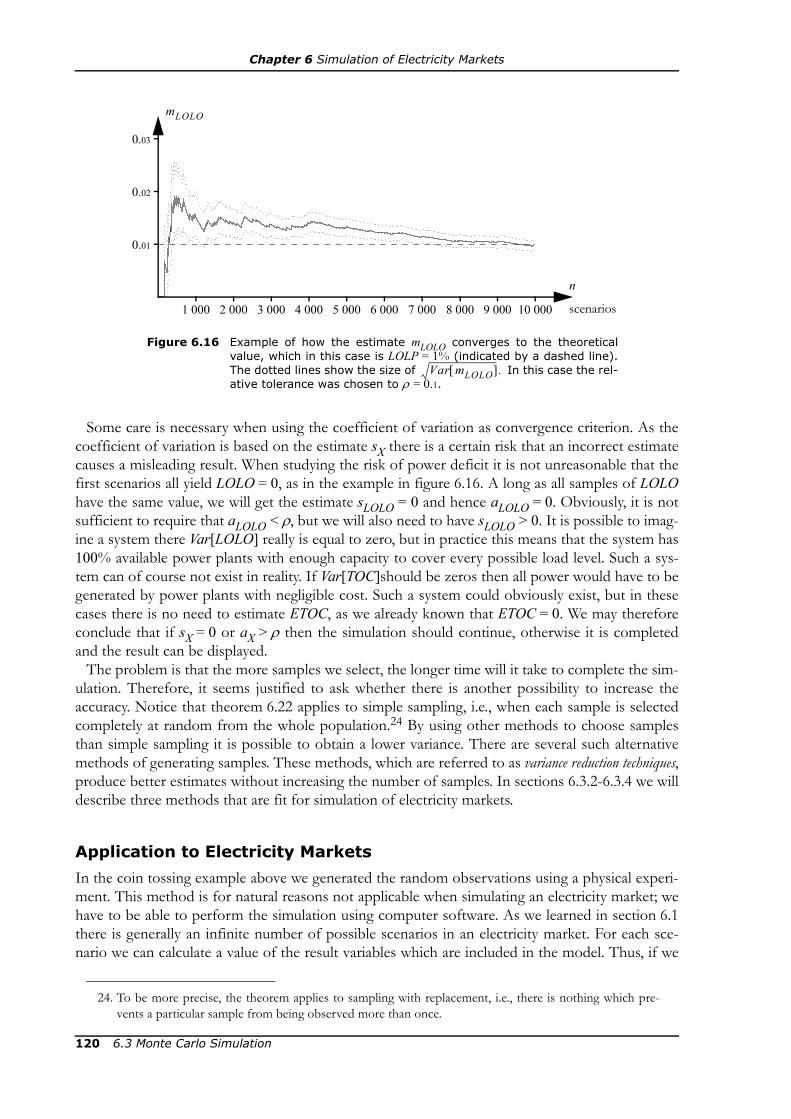
Chapter 6 Simulation of Electricity Markets
Some care is necessary when using the coefficient of variation as convergence criterion. As thecoefficient of variation is based on the estimate sX there is a certain risk that an incorrect estimatecauses a misleading result. When studying the risk of power deficit it is not unreasonable that thefirst scenarios all yield LOLO = 0, as in the example in figure 6.16. A long as all samples of LOLOhave the same value, we will get the estimate sLOLO = 0 and hence aLOLO = 0. Obviously, it is notsufficient to require that aLOLO < ρ, but we will also need to have sLOLO > 0. It is possible to imag-ine a system there Var[LOLO] really is equal to zero, but in practice this means that the system has100% available power plants with enough capacity to cover every possible load level. Such a sys-tem can of course not exist in reality. If Var[TOC]should be zeros then all power would have to begenerated by power plants with negligible cost. Such a system could obviously exist, but in thesecases there is no need to estimate ETOC, as we already known that ETOC = 0. We may thereforeconclude that if sX = 0 or aX > ρ then the simulation should continue, otherwise it is completedand the result can be displayed.
The problem is that the more samples we select, the longer time will it take to complete the sim-ulation. Therefore, it seems justified to ask whether there is another possibility to increase theaccuracy. Notice that theorem 6.22 applies to simple sampling, i.e., when each sample is selectedcompletely at random from the whole population.24 By using other methods to choose samplesthan simple sampling it is possible to obtain a lower variance. There are several such alternativemethods of generating samples. These methods, which are referred to as variance reduction techniques,produce better estimates without increasing the number of samples. In sections 6.3.2-6.3.4 we willdescribe three methods that are fit for simulation of electricity markets.
Application to Electricity Markets
In the coin tossing example above we generated the random observations using a physical experi-ment. This method is for natural reasons not applicable when simulating an electricity market; wehave to be able to perform the simulation using computer software. As we learned in section 6.1there is generally an infinite number of possible scenarios in an electricity market. For each sce-nario we can calculate a value of the result variables which are included in the model. Thus, if we
24. To be more precise, the theorem applies to sampling with replacement, i.e., there is nothing which pre-vents a particular sample from being observed more than once.
2 000 scenarios
n
1 000 3 000 4 000 5 000
mLOLO
0.03
0.02
0.01
7 0006 000 8 000 9 000 10 000
Figure 6.16 Example of how the estimate mLOLO converges to the theoreticalvalue, which in this case is LOLP = 1% (indicated by a dashed line).The dotted lines show the size of In this case the rel-ative tolerance was chosen to ρ = 0.1.
Var mLOLO[ ].
120 6.3 Monte Carlo Simulation

Chapter 6 Simulation of Electricity Markets
randomly create a scenario, we can use the electricity market model to calculate a sample of eachresult variable. For simplicity, we collect the outcomes of all scenario parameters in a vector Y,while we in a similar manner collect the values of all result variables in a vector X, i.e.,
X = g(Y),where g is the mathematical model of the electricity market (cf.section 6.1). Hence, simple sam-pling of an electricity market is equivalent to randomising n scenarios, y1, …, yn, calculate the resultvariables for each scenario and form the mean of the observed outcomes of the result variables,i.e.,
mX = (6.33)
To generate random scenarios we need a random number generator. A computer cannot gener-ate truly random numbers, but by using clever functions it is possible to use a start value—aseed—to generate a sequence of pseudorandom numbers. This sequence is assuredly determinis-tic, but for an outsider it is impossible to predict the next number in the sequence by just observ-ing the previous numbers. A good random number generates a sequence having approximately thesame statistical properties as a sequence of U(0, 1)-distributed random number.25 These randomnumbers can then be transformed to random number of the same probability distribution as thescenario parameters. It is recommended to use the inverse transform method (which is describedin appendix E) for this transformation.
Assume that we have an electricity market simulation with K scenario parameters and that n sce-narios are to be generated. The routine for applying simple sampling can then be summarised asfollows (cf. figure 6.17):
Step 1. Generate a random number uk, i and transform it according to the probabil-ity distribution of the scenario parameter k, i.e., let yk, i = Step 2. Repeat step 1 for each of the K scenario parameters and combine the out-comes to a vector yi. Calculate xi = g(yi).Step 3. Repeat step 1-2 for each of the n scenarios. Calculate
mX =
Let us now study a small example of simple sampling of an electricity market:Example 6.22 (simple sampling of a small power system). The SouthAmerican village Pueblo is not connected to the national grid, but has a local grid ofits own. The load in Pueblo is normally distributed with the mean 180 kW and stand-ard deviation 40 kW. The system is supplied by three power plants: a hydro power
Inversetransformmethod
SamplingU Y X mX
Figure 6.17 The principle of simple sampling.
Randomnumber
generator
Mathe-maticalmodel
25. By U(0, 1)-distributed random number we mean random numbers which can get a value between 0 and 1,and where all outcomes are equally probable.
1n--- xi
i 1=
n
∑ 1n--- g yi( ).
i 1=
n
∑=
FYk1– uk i,( ).
1n--- xi.
i 1=
n
∑
6.3 Monte Carlo Simulation 121

Chapter 6 Simulation of Electricity Markets
plant and two diesel generator sets. The hydro power plant is a run-of-the-river plant(i.e., there is no reservoir) and has an installed capacity of 150 kW. The least recordedwater flow in the river where the hydro power plant is located, was large enough torun the plant at installed capacity. The operation cost is negligible. The two diesel gen-erator sets are of 100 and 50 kW respectively. The larger generator has an operationcost of 1 ¤/kWh. However, the efficiency of this unit is very poor when it is onlypartly loaded, and it is therefore never operated at less than 40 kW. If it is necessary awater heater can be used to consume any surplus generation. The smaller diesel gener-ator set has an operation cost of 2 ¤/kWh. All units have an availability of 100%.Determine the ETOC of the system and verify the result.Solution: Both available capacity and operation cost of the power generators are fixedand can therefore be considered model constants.The only scenario parameter in thissystem is then the load, D. The objective of the simulation is to determine ETOC,which implies that we need to generate samples of the result variable TOC. The elec-tricity market model g should therefore describe the relation between the load and thetotal operation cost. We assume that the system is operated so that the operation costis minimised and that everything possible is done to avoid disconnection of consum-ers. This means that the system is operated as described in table 6.8. Using this strat-egy, we can draw the function TOC = g(D) as in figure 6.18. In this simple example of a Monte Carlo simulation we limit ourselves to creating 10scenarios, which in this case corresponds to randomising 10 values of the load (referto appendix E for a description of how random numbers of an arbitrary distributioncan be created). Then we calculate the mean of the operation cost for these ten sam-ples. Using appropriate software we obtain the ten scenarios listed in table 6.9. (Theten samples are also indicated in figure 6.18.) The estimate of the expectation value ofthe operation cost is therefore
=
= (40.0 + 0 + 62.1 + 0 + 49.0 + 64.8 + 75.0 + 61.3 + 31.1 + 42.8)/10 ≈ 42.61.
Table 6.8 Model of the power system operation in Pueblo.
D [kW] TOC [¤/h] Comment
0 - 150 0 The hydro power plant follows the load.
150 - 170 2·(D – 150) The hydro power plant is operated at full capacity.The small diesel generator follows the load.
170 - 190 40The hydro power plant is operated at full capacity.The large diesel generator set is operated at 40 kW.Surplus generation is consumed by the water heater.
190 - 250 (D – 150) The hydro power plant is operated at full capacity.The large diesel generator set follows the load.
250 - 300 100 + 2·(D-250)The hydro power plant is operated at full capacity.The large diesel generator set is operated at full capacity.The small diesel generator set follows the load.
> 300 200 All units are operated at full capacity.Some consumption is disconnected.a
a. As nothing else is stated in the assignment, we assume that no compensation is paid to those affected.
mTOC110------ TOCi
i 1=
10
∑=
122 6.3 Monte Carlo Simulation
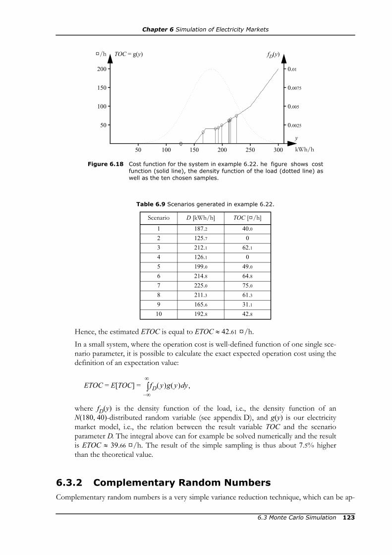
Chapter 6 Simulation of Electricity Markets
Hence, the estimated ETOC is equal to ETOC ≈ 42.61 ¤/h.In a small system, where the operation cost is well-defined function of one single sce-nario parameter, it is possible to calculate the exact expected operation cost using thedefinition of an expectation value:
ETOC = E[TOC] =
where fD(y) is the density function of the load, i.e., the density function of anN(180, 40)-distributed random variable (see appendix D), and g(y) is our electricitymarket model, i.e., the relation between the result variable TOC and the scenarioparameter D. The integral above can for example be solved numerically and the resultis ETOC ≈ 39.66 ¤/h. The result of the simple sampling is thus about 7.5% higherthan the theoretical value.
6.3.2 Complementary Random NumbersComplementary random numbers is a very simple variance reduction technique, which can be ap-
Figure 6.18 Cost function for the system in example 6.22. he figure shows costfunction (solid line), the density function of the load (dotted line) aswell as the ten chosen samples.
100 kWh/h
y
50 150 200 250
200
100
50
150
¤/h TOC = g(y)
300
0.01
0.005
0.0025
0.0075
fD(y)
Table 6.9 Scenarios generated in example 6.22.
Scenario D [kWh/h] TOC [¤/h]
1 187.2 40.02 125.7 03 212.1 62.14 126.1 05 199.0 49.06 214.8 64.87 225.0 75.08 211.3 61.39 165.6 31.110 192.8 42.8
fD y( )g y( ) y,d∞–
∞
∫
6.3 Monte Carlo Simulation 123

Chapter 6 Simulation of Electricity Markets
plied in all kinds of Monte Carlo simulations. The technique is based on modifying the randomnumber generator so that it generates series of random values which are not independent. Theconsequence is that less samples are necessary to get a good spread of the samples.
Theory
Assume that mX1 and mX2 are two estimates of the expectation value, μX, of a certain random var-iable, i.e., E[mX1] = E[mX2] = E[X] = μX. If we consider the average of mX1 and mX2 we find thatthe expectation value is
(6.34)
Hence, the average of mX1 and mX2 is also an estimate of μX, which maybe is not very surprising.However, the interesting is that the variance of the average is
(6.35)
The variance of the average is, as can be seen, less than the variance of mX1 and mX2respectively.Above all, it is possible to utilise that the covariance can become negative. A simple way of creat-ing estimates with a negative covariance is to use complementary random numbers.
Random numbers of any probability distribution can be created by transformation of U(0, 1)-distributed random numbers (see appendix E). If U is U(0, 1)-distributed then the complementaryrandom number of U is given by U* = 1 – U. We can see that U* also is a U(0, 1)--distributed ran-dom variable. If the outcome of U is high then U* will receive a low value and vice versa, whichobviously means that U and U* are negatively correlated. If Y is a random variable from an arbi-trary probability distribution and Y has been obtained by transforming U, and Y* is obtained byapplying the same transformation on U*, then Y and Y* will be negatively correlated.
Example 6.23 (random complement of a normally distributed randomvariable): Randomise a sample from an N(5, 2)-distribution. Calculate the comple-mentary random number of this sample.Solution: Normally distributed random variables can, as described in appendix E, beobtained by transformation of random number from a U(0, 1)-distribution. Assumethat we start with U = 0.15. Using theorem E.2 we get Y ≈ –1.04, which is an N(1, 0)-distributed random number. This value is transformed to the desired normal distribu-tion using theorem D.3, which yields 5 + 2·(–1.04) ≈ 2.93.The random complement is obtained by performing the same transformations onU* = 1 – 0.15, which corresponds to 7.07 rom the desired normal distribution. Consid-ering that the normal distribution is symmetrical it is logical that Y* is as much higherthan the mean value as Y is smaller than the mean.
Application to Electricity Markets
Complementary random numbers are very straightforward to apply when simulating electricitymarkets. Assume that n scenarios yi has been generated and that the complementary randomnumber, yi* is calculated for each scenario. When the result variables are calculated both for theoriginal scenarios and those based on complementary random numbers. Notice that as we in gen-eral will have more than one scenario parameter in an electricity market simulation, we will obtainmore than one scenario based on complementary random numbers. Each scenario parameter willhave two possible values: the original value and its complement. The original values and comple-
EmX1 mX2+
2-------------------------- 1
2---E mX1[ ] 1
2---E mX2[ ]+ μX.= =
VarmX1 mX2+
2-------------------------- 1
4---Var mX1[ ] 1
4---Var mX2[ ] 1
2---Cov mX1 mX2,[ ].+ +=
124 6.3 Monte Carlo Simulation
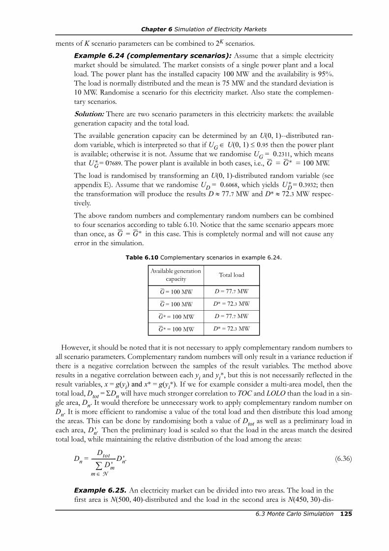
Chapter 6 Simulation of Electricity Markets
ments of K scenario parameters can be combined to 2K scenarios. Example 6.24 (complementary scenarios): Assume that a simple electricitymarket should be simulated. The market consists of a single power plant and a localload. The power plant has the installed capacity 100 MW and the availability is 95%.The load is normally distributed and the mean is 75 MW and the standard deviation is10 MW. Randomise a scenario for this electricity market. Also state the complemen-tary scenarios.Solution: There are two scenario parameters in this electricity markets: the availablegeneration capacity and the total load.The available generation capacity can be determined by an U(0, 1)--distributed ran-dom variable, which is interpreted so that if UG ∈ U(0, 1) ≤ 0.95 then the power plantis available; otherwise it is not. Assume that we randomise UG = 0.2311, which meansthat = 07689. The power plant is available in both cases, i.e., = = 100 MW.The load is randomised by transforming an U(0, 1)-distributed random variable (seeappendix E). Assume that we randomise UD = 0.6068, which yields = 0.3932; thenthe transformation will produce the results D ≈ 77.7 MW and D* ≈ 72.3 MW respec-tively.The above random numbers and complementary random numbers can be combinedto four scenarios according to table 6.10. Notice that the same scenario appears morethan once, as = in this case. This is completely normal and will not cause anyerror in the simulation.
However, it should be noted that it is not necessary to apply complementary random numbers toall scenario parameters. Complementary random numbers will only result in a variance reduction ifthere is a negative correlation between the samples of the result variables. The method aboveresults in a negative correlation between each yi and yi*, but this is not necessarily reflected in theresult variables, x = g(yi) and x* = g(yi*). If we for example consider a multi-area model, then thetotal load, Dtot = ΣDn will have much stronger correlation to TOC and LOLO than the load in a sin-gle area, Dn. It would therefore be unnecessary work to apply complementary random number onDn. It is more efficient to randomise a value of the total load and then distribute this load amongthe areas. This can be done by randomising both a value of Dtot as well as a preliminary load ineach area, Then the preliminary load is scaled so that the load in the areas match the desiredtotal load, while maintaining the relative distribution of the load among the areas:
Dn = (6.36)
Example 6.25. An electricity market can be divided into two areas. The load in thefirst area is N(500, 40)-distributed and the load in the second area is N(450, 30)-dis-
Table 6.10 Complementary scenarios in example 6.24.
Available generation capacity Total load
= 100 MW D = 77.7 MW
= 100 MW D* = 72.3 MW
= 100 MW D = 77.7 MW
= 100 MW D* = 72.3 MW
UG* G G*
UD*
G G*
G
G
G*
G*
Dn'.
DtotDm'
m N∈∑
--------------------Dn'.
6.3 Monte Carlo Simulation 125

Chapter 6 Simulation of Electricity Markets
tributed. The load level in the two areas are independent random variables. Generatetwo scenarios for this electricity market in such a way that the total load in the secondscenario is equal to the complementary random number of the total load in the firstscenario. Use the following five random numbers from an N(0, 1)-distribution: 1.65,–0.74, 0.27, –0.04 and 1.23.Solution: We start by establishing the fact that the total load is the sum of two nor-mally distributed random variables; hence, the total load is normally distributed andhas a mean of 500 + 450 = 950 and the standard deviation = 50. We cannow use theorem D.3 to transform the given random numbers to the appropriate nor-mal distribution. We may start by transforming the first random number into a valueof the total load, which results in Dtot = 950 + 50 · 1.65 = 1 032.5 MW. As the normaldistribution is symmetrical, we then get the complementary random numberDtot* = 950 – 50 · 1.65 = 867.5 MW.The next two random numbers are transformed into preliminary values of the load inthe two areas for the first scenario:D1
i = 500 + 40 · (–0.74) = 470.4 MW and D2i = 400
+ 30 · 0.27 = 408.1 MW. Then these values are scaled to match the desired value of thetotal load in the first scenario:
D1 = ≈ 552.9 MW,
D2 = ≈ 479.6 MW.
Finally, we use the last two random values to generate preliminary values of the load inthe two areas for the second scenario: D1
ii = 500 + 40 · (–0.04) = 498.4 MW andD2
ii = 400 + 30 · 1.23 = 436.9 MW. This time the preliminary load is scaled so that thesum equals the complementary random number of the total load in the first scenario,which means that we get the following area loads:
D1 = ≈ 462.3 MW,
D2 = ≈ 405.2 MW.
Assume that we have an electricity market simulation with K scenario parameters (out of whichKV scenario parameters are such that it makes sense to apply complementary random numbers)and that n scenarios are to be generated. The routine for applying complementary random num-bers can then be summarised as follows (cf. figure 6.19):
Step 1. Generate a random number uk, i and transform it according to the probabil-ity distribution of the scenario parameter k, i.e., let yk, i = If applicable tothis scenario parameter, also transform the complementary random number i.e., let = Step 2. Repeat step 1 for each of the K scenario parameters. Create 2K complemen-
402 302+
1 032.5470.4 408.1+( )
-------------------------------------470.4
1 032.5470.4 408.1+( )
-------------------------------------408.1
867.5498.4 436.9+( )
-------------------------------------498.4
867.5498.4 436.9+( )
-------------------------------------436.9
U Y XmX
Figure 6.19 The principle of complementary random numbers.
U* Y* X*Inverse
transformmethod
SamplingRandomnumber
generator
Mathe-maticalmodel
FYk1– uk i,( ).
yk i,*FYk
1– 1 u– k i,( ).
126 6.3 Monte Carlo Simulation
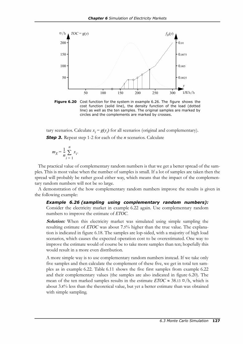
Chapter 6 Simulation of Electricity Markets
tary scenarios. Calculate xi = g(yi) for all scenarios (original and complementary).Step 3. Repeat step 1-2 for each of the n scenarios. Calculate
mX =
The practical value of complementary random numbers is that we get a better spread of the sam-ples. This is most value when the number of samples is small. If a lot of samples are taken then thespread will probably be rather good either way, which means that the impact of the complemen-tary random numbers will not be so large.
A demonstration of the how complementary random numbers improve the results is given inthe following example:
Example 6.26 (sampling using complementary random numbers):Consider the electricity market in example 6.22 again. Use complementary randomnumbers to improve the estimate of ETOC.Solution: When this electricity market was simulated using simple sampling theresulting estimate of ETOC was about 7.5% higher than the true value. The explana-tion is indicated in figure 6.18. The samples are lop-sided, with a majority of high loadscenarios, which causes the expected operation cost to be overestimated. One way toimprove the estimate would of course be to take more samples than ten; hopefully thiswould result in a more even distribution.A more simple way is to use complementary random numbers instead. If we take onlyfive samples and then calculate the complement of these five, we get in total ten sam-ples as in example 6.22. Table 6.11 shows the five first samples from example 6.22and their complementary values (the samples are also indicated in figure 6.20). Themean of the ten marked samples results in the estimate ETOC ≈ 38.13 ¤/h, which isabout 3.8% less than the theoretical value, but yet a better estimate than was obtainedwith simple sampling.
1n--- xi.
i 1=
n
∑
Figure 6.20 Cost function for the system in example 6.26. The figure shows thecost function (solid line), the density function of the load (dottedline) as well as the ten samples. The original samples are marked bycircles and the complements are marked by crosses.
100 kWh/h
y
50 150 200 250
200
100
50
150
¤/h TOC = g(y)
300
0.01
0.005
0.0025
0.0075
fD(y)
6.3 Monte Carlo Simulation 127

Chapter 6 Simulation of Electricity Markets
6.3.3 Control VariatesOne of the most important reasons to use Monte Carlo methods is that they can manage modelswhich are too complex to be treated analytically. However, using control variates, it becomes pos-sible to use simplified analytical models to improve the result of the Monte Carlo-simulation.
Theory
Assume that X is a random variable with a certain expectation value i.e., E[X] = Moreo-ver, assume that there is another random variable, a control variate Z, the expectation value of which,E[Z]= is known (through analytical calculations or from earlier investigations). Rather than es-timating E[X] we choose to estimate the expected difference between X and Z. An estimate of E[X]is then calculated by
mX = m(X – Z) + μZ, (6.37)
becauseE[m(X – Z) + μZ] = E[X – Z] + μZ = E[X] – μZ + μZ = μX. (6.38)
The variance of the difference X – Z isVar[X – Z] = Var[X] + Var[Z] – 2Cov[X, Z]. (6.39)
If we can find a control variate Z which has a strong positive correlation to X then it is possiblethat 2Cov[X, Z] > Var[Z]; hence, X – Z may have a lower variance than X. Simple sampling of X – Zis then according to theorem 6.22 resulting in a smaller variance of the estimate than if X is sam-pled directly.
Application to Electricity Markets
The prerequisite of applying control variates is that there is an analytical model to compare with.For each scenario generated in the Monte Carlo simulation, we calculate the result variables of thedetailed model, i.e.,
X = g(Y), (6.40a)as well as the analytical model, i.e.,
Z = (6.40b)
A suitable analytical model to be used in electricity market simulations is a single-area model,where the load is not price sensitive and the electricity market is in every scenario assumed to min-imise the total operation cost while maintaining balance between generation and consumption.
Table 6.11 Scenarios generated in example 6.23.
Scenario D [kWh/h] TOC [¤/h] D* [kWh/h] TOC* [¤/h]
1 187.2 40.0 172.8 40.02 125.7 0 234.3 84.33 212.1 62.1 147.9 04 126.1 0 233.9 83.95 199.0 49.0 161.0 22.0
μX, μX.
μZ,
g Y( ).
128 6.3 Monte Carlo Simulation

Chapter 6 Simulation of Electricity Markets
Such a model can be defined from the solution to the following, simple LP problem:
minimise (6.41)
subject to (6.41a)
0 ≤ ≤ ∀ g ∈ G, (6.41b)
0 ≤ (6.41c)
In the optimisation problem (6.41) we have the following variables:= generation in power plant g,= unserved power.
The parameters areDtot = total load,
= available generation capacity in power plant g,βg = generation cost in power plant g,βU = penalty cost for unserved power.26
From the solution to (6.41) we can define the control variates
(6.42a)
(6.42b)
It should be noted that the optimisation problem (6.41) is very straightforward to solve by handcalculations. The power plants are sorted in a merit order according to ascending cost. Then thegeneration in the least expensive power plant is increased until it either covers the load or reachesits available capacity. In the latter case we proceed and try with the next power plant, etc. As a lastresort we use load shedding to balance the constraint (6.41a).
Since the model in (6.41) corresponds to the model used in probabilistic production cost simula-tion; thus, the expectation value of the control variates can be calculated using the methodsdescribed in section 6.2.
Assume that we have an electricity market simulation with K scenario parameters and that n sce-narios are to be generated. The routine for applying control variates can then be summarised asfollows (cf. figure 6.21):
Step 1. Generate a random number uk, i and transform it according to the probabil-ity distribution of the scenario parameter k, i.e., let yk, i = Step 2. Repeat step 1 for each of the K scenario parameters and combine the out-comes to a vector yi. Calculate the result variables xi = g(yi) and the control variateszi =Step 3. Repeat step 1-2 for each of the n scenarios. Calculate
26. As in the multi-area problem from section 6.1.1, we are here forced to introduce a possibly fictitious costfor load shedding in order to prevent the load balance to be maintained by disconnecting all load, eventhough there is unused generation capacity available.
βgGg βUU+g G∈∑
Gg U+g G∈∑ Dtot,=
Gg Gg,
U.
Gg
U
Gg
TOC˜ βgGg,g G∈∑=
LOLO˜ 1 if U 0,>0 otherwise.⎩
⎨⎧
=
FYk1– uk i,( ).
g yi( ).
6.3 Monte Carlo Simulation 129

Chapter 6 Simulation of Electricity Markets
mX – Z =
Step 4. Calculate μZ = E[Z].
Step 5. Calculate mX = mX – Z + μZ.
The principle of applying a control variate is illustrated in the following example:Example 6.27 (sampling using a control variate). Consider the electricitymarket from example 6.22 once again. Use a control variate to improve the estimateof ETOC.Solution: The same ten samples were used as in example 6.22. However, in this casethe value of samples is equal to the difference between the detailed model, g(D), andthe simplified model, Let us denote this difference by TOCD, i.e., TOCD = TOC
U mX – Z
Figure 6.21 The principle of control variates.
Y
X
Z
+
–
mX
μZ
++Inverse
transformmethod
SamplingRandomnumber
generator
Mathmati-cal model(detailed)
Mathmati-cal model
(simplified)
1n--- xi zi–( ) .
i 1=
n
∑
Figure 6.22 Cost function for the system in example 6.27. The figure shows costfunction for the detailed model (solid line), cost function for a PPCmodel (dashed line)—notice that these lines coincide except for asmall interval. The figure also shows the ten samples, which consti-tute the difference between the solid and the dashed lines. Finally,the density function of the load is shown (dotted line).
100 kWh/h
y
50 150 200 250
200
100
50
150
¤/h TOC = g(y)
300
0.01
0.005
0.0025
0.0075
fD(y)
g D( ).
130 6.3 Monte Carlo Simulation

Chapter 6 Simulation of Electricity Markets
– As we can see in table 6.12, the two models only differ in two cases. Themean of the ten samples is 1.84 ¤/h, which means that we obtain the estimatemTOCD = 1.84 ¤/h. By performing a probabilistic production cost simulation of thissystem we get ≈ 36.27 ¤/h. The estimate using a control variate is thus
mTOC = mTOCD + = 36.27 + 1.84 ≈ 38.11 ¤/h.
Hence, the control resulted in an improvement of the estimate which is about thesame as when we were using complementary random numbers in example 6.26. Tounderstand why the estimate is improved, we can study how the expectation values arecalculated with and without control variate:
ETOC = E[TOC] =
ETOC = E[TOCD] + =
Table 6.12 Scenarios generated in example 6.27.
Scenario D [kWh/h] TOC [¤/h] [¤/h] TOCD [¤/h]
1 187.2 40.0 37.2 2.82 125.7 0 0 03 212.1 62.1 62.1 04 126.1 0 0 05 199.0 49.0 49.0 06 214.8 64.8 64.8 07 225.0 75.0 75.0 08 211.3 61.3 61.3 09 165.6 31.1 15.6 15.610 192.8 42.8 42.8 0
TOC˜
TOC˜ .
μTOC˜
μTOC˜
100 kWh/h
y
50 150 200 250
0.5
0.3
0.2
0.4
¤/h integrand
300
Figure 6.23 Illustration of the integrand for calculation of the expectation valuewith and without control variate The solid line shows the integrandfD(y)g(y) and the dashed line shows The differencebetween them corresponds to the shaded area.
fD y( )g y( ).
0.1
fD y( )g y( ) y,d∞–
∞
∫
μTOC˜ fD y( ) g y( ) g y( )–( ) y μTOC˜ .+d
∞–
∞
∫
6.3 Monte Carlo Simulation 131

Chapter 6 Simulation of Electricity Markets
The integrands of these two expressions are shown in figure 6.23. ETOC correspondsto the area below the solid line, i.e., both the shaded and the white area, whereas theexpectation value of TOCD corresponds to just the shaded area. When using the con-trol variate, we try to estimate the shaded area, while the white area is given usingprobabilistic production cost simulation. An error of 10% in the Monte Carlo esti-mate will therefore affect the whole result when ETOC is estimated directly, but only asmall part of the result (the shaded area) when a control variate is used.
6.3.4 Stratified SamplingThe idea of stratified sampling is to divide the samples in different subpopulations which are re-ferred to as strata,27 and which are investigated separately. Some are practical (it may for examplebe so that different parts of a study must be performed using different methods), but there arealso possibilities to gain efficiency. If it is possible to collect samples having similar properties inthe same stratum then the variance within each stratum will be reduced. Since reduced variancemeans increased efficiency according to theorem 6.22, the result is that the expectation value ofthe samples within the stratum can be determined faster and/or more accurately. These expecta-tion values can then simply be weighted together to obtain an expectation value of the entire pop-ulation.
Theory
Assume that we have a random variable X with the sample space 28 X. In stratified sampling thesample space is divided in L strata, where stratum h comprises the outcomes Xh, which is a subsetof X. Strata may not overlap, i.e., each outcome must belong to exactly one stratum:
= ∅, (6.43a)
Xh ∩ Xj = ∅ ∀ h ≠ j. (6.43b)
Each stratum is assigned a weight corresponding to how large part of the population which be-longs to the stratum:
ωh = = P(X ∈ Xh), (6.44)
where
ωh = stratum weight of stratum h,Nh = number of units (i.e., possible outcomes) in stratum h,N = number of units in the entire population.
As can be seen above, the stratum weight can also be considered as the probability that a randomobservation of X will fall into stratum h.
Is is now possible to consider L separate random variables Xh, h = 1, …, L, each with the samplespace Xh. The expectation value of each stratum is calculated separately. In some cases it might bepossible to analytically determine E[Xh]; if not, we can estimate it by simple sampling:
27. This footnote has just been added to maintain the footnote numbering in pace with the Swedish edition.28. The sample space is the set of possible outcomes of X.
Xhh∪
NhN------
132 6.3 Monte Carlo Simulation
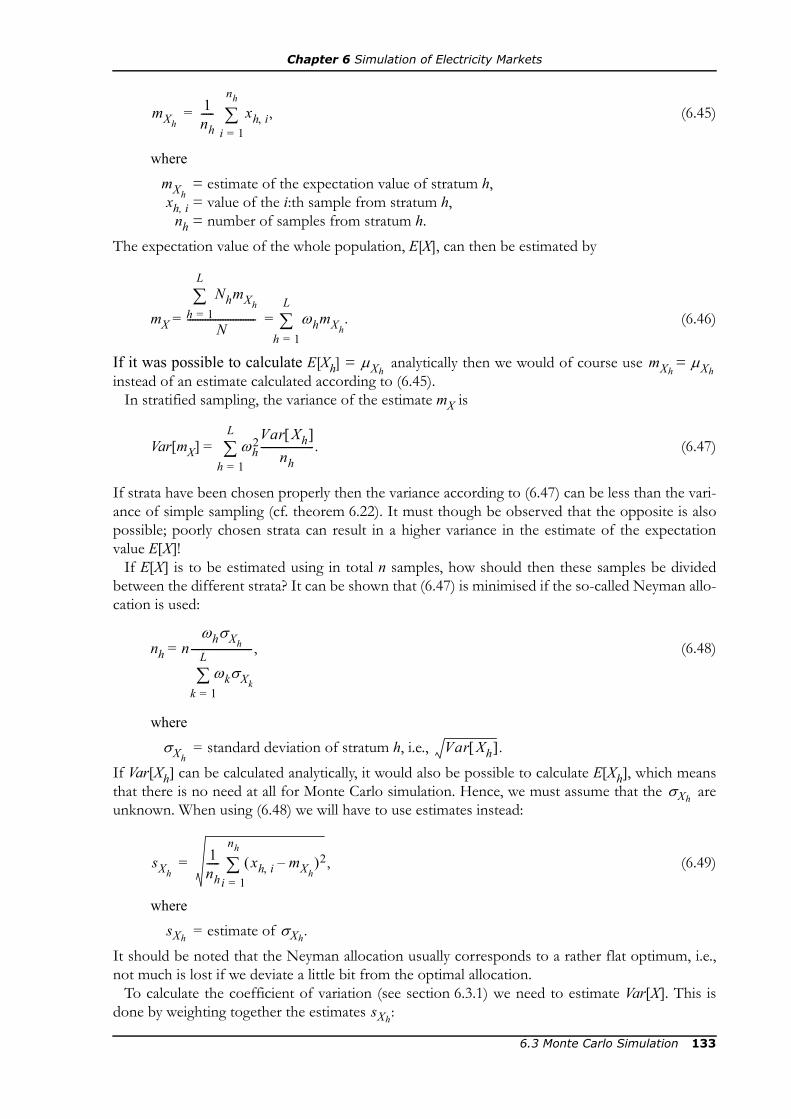
Chapter 6 Simulation of Electricity Markets
(6.45)
where
= estimate of the expectation value of stratum h,xh, i = value of the i:th sample from stratum h,
nh = number of samples from stratum h.The expectation value of the whole population, E[X], can then be estimated by
mX = (6.46)
If it was possible to calculate E[Xh] = analytically then we would of course use =instead of an estimate calculated according to (6.45).
In stratified sampling, the variance of the estimate mX is
Var[mX] = (6.47)
If strata have been chosen properly then the variance according to (6.47) can be less than the vari-ance of simple sampling (cf. theorem 6.22). It must though be observed that the opposite is alsopossible; poorly chosen strata can result in a higher variance in the estimate of the expectationvalue E[X]!
If E[X] is to be estimated using in total n samples, how should then these samples be dividedbetween the different strata? It can be shown that (6.47) is minimised if the so-called Neyman allo-cation is used:
nh = (6.48)
where
= standard deviation of stratum h, i.e., If Var[Xh] can be calculated analytically, it would also be possible to calculate E[Xh], which meansthat there is no need at all for Monte Carlo simulation. Hence, we must assume that the areunknown. When using (6.48) we will have to use estimates instead:
(6.49)
where
= estimate of It should be noted that the Neyman allocation usually corresponds to a rather flat optimum, i.e.,not much is lost if we deviate a little bit from the optimal allocation.
To calculate the coefficient of variation (see section 6.3.1) we need to estimate Var[X]. This isdone by weighting together the estimates
mXh
1nh----- xh i,
i 1=
nh
∑ ,=
mXh
NhmXhh 1=
L
∑
N--------------------------- ωhmXh
.h 1=
L
∑=
μXhmXh
μXh
ωh2Var Xh[ ]
nh--------------------- .
h 1=
L
∑
nωhσXh
ωkσXkk 1=
L
∑------------------------ ,
σXhVar Xh[ ].
σXh
sXh
1nh----- xh i, mXh
–( )2
i 1=
nh
∑ ,=
sXh σXh.
sXh:
6.3 Monte Carlo Simulation 133

Chapter 6 Simulation of Electricity Markets
(6.50)
Application to Electricity Markets
Before stratified sampling can be used in a simulation of an electricity market the strata have to bedefined. As mentioned in the theory section above, an inappropriate stratification may result in aless accurate result than when using simple sampling; hence, strata need to be chosen carefully. Wewill return to this issue in section 6.3.5; for now we restrict ourselves to discussing how stratifiedsampling is applied given a specific stratification.
Assume that we have an electricity market simulation with K scenario parameters and L strata,and that nh scenarios are to be generated from each stratum. The routine for applying stratifiedsampling can then be summarised as follows (cf. figure 6.24):
Step 1. Consider stratum h. If possible, calculate E[Xh] = μXh using analytical meth-ods, set mXh = μXh and proceed to step 5. Step 2. Generate a random number uk, h, i and transform it according to the proba-bility distribution in stratum h of the scenario parameter k, i.e., let yk, h, i =
Step 3. Repeat step 2 for each of the K scenario parameters and combine the out-comes to a vector yh,i. Calculate xh, i = g(yh, i).Step 4. Repeat step 2-3 for each of the nh scenarios. Calculate
mXh =
sX2 ωh
2sXh2 .
h 1=
L
∑=
Figure 6.24 The principle of stratified sampling. The expectation value ofeach stratum is estimated by simple sampling (as in the top andbottom strata in the figure) or is known from analytical calcula-tions (as in the middle stratum).
mX1
+
U Y1 X1
ω1
μXh+
ωh+
ωL
…
…
mXLU YL XL
mX
Inversetransformmethod
SamplingRandomnumber
generator
Mathe-maticalmodel
Inversetransformmethod
SamplingRandomnumber
generator
Mathe-maticalmodel
FYk h,1– uk h i, ,( ).
1nh----- xh i, .
i 1=
nh
∑
134 6.3 Monte Carlo Simulation

Chapter 6 Simulation of Electricity Markets
Step 5. Repeat step 1-4 for each of the L strata.
Step 6. Calculate mX =
The following example demonstrates how stratified sampling is used in a simulation of an elec-tricity market:
Example 6.28 (stratified sampling). Again we will study the electricity marketfrom example 6.22. Use stratified sampling to improve the estimate of ETOC.Solution: It is important to define strata and choose number of samples per stratumin a wise manner in order to get good results from stratified sampling. For themoment we will however make these decision based on engineer’s intuition. There-fore, let stratum 1 be all scenarios where the load is less then or equal to 150 kW, stra-tum 2 is the scenarios where the load is higher than 150 kW but less than 250 kW andfinally stratum 3 consists of all other load levels. Then we generate two scenarios eachfrom stratum 1 and 3, while the remaining six samples are allocated to stratum 2. Thechosen scenarios and the stratum boundaries are shown in table 6.13 and are also indi-cated in figure 6.25. The expectation value of each stratum is
ETOC1 = 0,
ETOC2 ≈ 45,73,
ETOC3 ≈ 136,23.
In order to estimate ETOC we also need the stratum weights. According to (6.44) weget
ω1 = P(D ≤ 150) = Φ((150 – 180)/40) ≈ 0.23,
ω2 = P(150 < D ≤ 250) = Φ((250 – 180)/40) – Φ((150 – 180)/40) ≈ 0.73,
ω3 = P(D > 250) = 1 – Φ((250 – 180)/40) ≈ 0.04.
The estimate of the whole population is then according to (6.46) ETOC ≈ 38.99 ¤/hor about 1.7% less than the true value. Thus, also stratified sampling provided a defi-
ωhmXh.
h 1=
L
∑
Figure 6.25 Cost function for the system in example 6.28. The figure shows thecost function (solid line) as well as the density function of the load(dotted line) and the ten chosen samples.The stratum boundariesare indicated by dash-dotted lines.
100 kWh/h
y
50 150 200 250
200
100
50
150
¤/h TOC = g(y)
300
0.01
0.005
0.0025
0.0075
fD(y)
6.3 Monte Carlo Simulation 135

Chapter 6 Simulation of Electricity Markets
nitely better estimate of the operation cost. There are two reasons why stratified sam-pling improves the result. One is that it is possible to define homogenous strata, ie.e.,strata where the individual deviations between the units which belong to the strata aresmall; thereby, few samples are required to obtain a good estimate of the expectationvalue for that stratum. In this case TOC is equal to zero for all scenarios in stratum 1.The second explanation it is possible to use few sample in less important strata, whichresult in less accurate estimates for those strata, but that will not affect the final resultvery much. In the example above the estimate of ETOC3 is rather poor (the true valueis 131.54 ¤/h, i.e., the estimate above is 3.5% too high), but this error does not have alarge impact on the final result, because stratum 3 has much lower stratum weightthan the other two strata.
6.3.5 Monte Carlo Simulation of Electricity MarketsTo complete our presentation concerning Monte Carlo simulation of electricity markets, we willaddress some further aspects. More precisely, we will discuss how several variance reduction tech-niques can be combined and we will provide some more details about how stratified samplingshould be applied.
Combining Several Variance Reduction Techniques
It is perfectly possible to combine the three variance reduction techniques described in the previ-ous sections. The procedure is demonstrated in the following example:
Example 6.29 (simulation using a combination of three variancereduction techniques). Consider the electricity market in example 6.22 again.What is the estimate of ETOC when all three variance reduction techniques areapplied simultaneously?Solution: We use the same stratification as in example 6.28. From strata 1 and 3 threewe create one original scenario and one complementary scenario each. In stratum 3we create three original scenarios and thereby obtain three complementary scenarios.The selected samples are shown in table 6.14 and are also indicated in figure 6.26. Thefollowing estimates are obtained in each stratum:
ETOCD1 = 0,
Table 6.13 Scenarios generated in example 6.28.
Stratum Scenario D [kWh/h] TOC [¤/h]
11 134.8 02 143.9 0
2
1 158.0 15.92 214.4 64.43 158.1 16.24 224.0 74.05 213.8 63.86 179.0 40.0
31 269.4 138.82 266.8 133.6
136 6.3 Monte Carlo Simulation
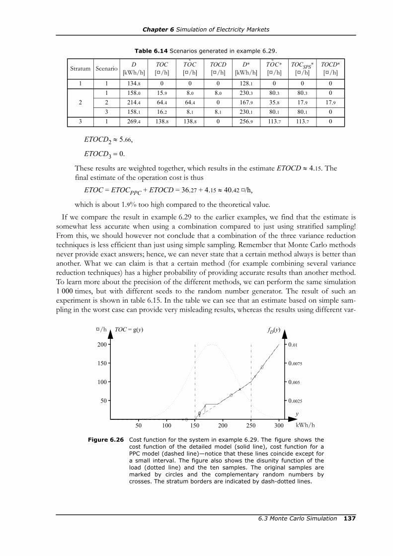
Chapter 6 Simulation of Electricity Markets
ETOCD2 ≈ 5.66,
ETOCD3 = 0.
These results are weighted together, which results in the estimate ETOCD ≈ 4.15. Thefinal estimate of the operation cost is thus
ETOC = ETOCPPC + ETOCD = 36.27 + 4.15 ≈ 40.42 ¤/h,
which is about 1.9% too high compared to the theoretical value. If we compare the result in example 6.29 to the earlier examples, we find that the estimate is
somewhat less accurate when using a combination compared to just using stratified sampling!From this, we should however not conclude that a combination of the three variance reductiontechniques is less efficient than just using simple sampling. Remember that Monte Carlo methodsnever provide exact answers; hence, we can never state that a certain method always is better thananother. What we can claim is that a certain method (for example combining several variancereduction techniques) has a higher probability of providing accurate results than another method.To learn more about the precision of the different methods, we can perform the same simulation1 000 times, but with different seeds to the random number generator. The result of such anexperiment is shown in table 6.15. In the table we can see that an estimate based on simple sam-pling in the worst case can provide very misleading results, whereas the results using different var-
100 kWh/h
y
50 150 200 250
200
100
50
150
¤/h TOC = g(y)
300
0.01
0.005
0.0025
0.0075
fD(y)
Figure 6.26 Cost function for the system in example 6.29. The figure shows thecost function of the detailed model (solid line), cost function for aPPC model (dashed line)—notice that these lines coincide except fora small interval. The figure also shows the disunity function of theload (dotted line) and the ten samples. The original samples aremarked by circles and the complementary random numbers bycrosses. The stratum borders are indicated by dash-dotted lines.
Table 6.14 Scenarios generated in example 6.29.
Stratum Scenario D [kWh/h]
TOC [¤/h]
[¤/h]
TOCD [¤/h]
D* [kWh/h]
[¤/h]
TOCSPS* [¤/h]
TOCD* [¤/h]
1 1 134.8 0 0 0 128.1 0 0 0
21 158.0 15.9 8.0 8.0 230.3 80.3 80.3 02 214.4 64.4 64.4 0 167.9 35.8 17.9 17.93 158.1 16.2 8.1 8.1 230.1 80.1 80.1 0
3 1 269.4 138.8 138.8 0 256.9 113.7 113.7 0
TOC˜ TOC˜ *
6.3 Monte Carlo Simulation 137
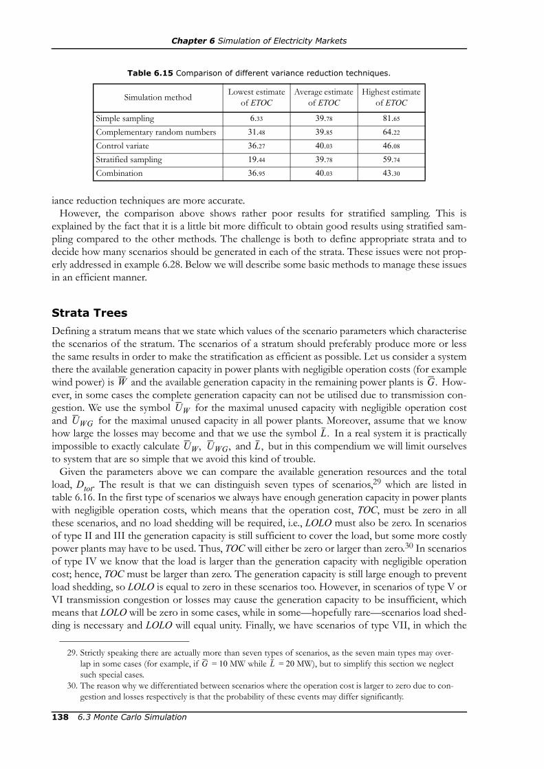
Chapter 6 Simulation of Electricity Markets
iance reduction techniques are more accurate.However, the comparison above shows rather poor results for stratified sampling. This is
explained by the fact that it is a little bit more difficult to obtain good results using stratified sam-pling compared to the other methods. The challenge is both to define appropriate strata and todecide how many scenarios should be generated in each of the strata. These issues were not prop-erly addressed in example 6.28. Below we will describe some basic methods to manage these issuesin an efficient manner.
Strata Trees
Defining a stratum means that we state which values of the scenario parameters which characterisethe scenarios of the stratum. The scenarios of a stratum should preferably produce more or lessthe same results in order to make the stratification as efficient as possible. Let us consider a systemthere the available generation capacity in power plants with negligible operation costs (for examplewind power) is and the available generation capacity in the remaining power plants is How-ever, in some cases the complete generation capacity can not be utilised due to transmission con-gestion. We use the symbol for the maximal unused capacity with negligible operation costand for the maximal unused capacity in all power plants. Moreover, assume that we knowhow large the losses may become and that we use the symbol In a real system it is practicallyimpossible to exactly calculate and but in this compendium we will limit ourselvesto system that are so simple that we avoid this kind of trouble.
Given the parameters above we can compare the available generation resources and the totalload, Dtot. The result is that we can distinguish seven types of scenarios,29 which are listed intable 6.16. In the first type of scenarios we always have enough generation capacity in power plantswith negligible operation costs, which means that the operation cost, TOC, must be zero in allthese scenarios, and no load shedding will be required, i.e., LOLO must also be zero. In scenariosof type II and III the generation capacity is still sufficient to cover the load, but some more costlypower plants may have to be used. Thus, TOC will either be zero or larger than zero.30 In scenariosof type IV we know that the load is larger than the generation capacity with negligible operationcost; hence, TOC must be larger than zero. The generation capacity is still large enough to preventload shedding, so LOLO is equal to zero in these scenarios too. However, in scenarios of type V orVI transmission congestion or losses may cause the generation capacity to be insufficient, whichmeans that LOLO will be zero in some cases, while in some—hopefully rare—scenarios load shed-ding is necessary and LOLO will equal unity. Finally, we have scenarios of type VII, in which the
Table 6.15 Comparison of different variance reduction techniques.
Simulation method Lowest estimate of ETOC
Average estimate of ETOC
Highest estimate of ETOC
Simple sampling 6.33 39.78 81.65
Complementary random numbers 31.48 39.85 64.22
Control variate 36.27 40.03 46.08
Stratified sampling 19.44 39.78 59.74
Combination 36.95 40.03 43.30
29. Strictly speaking there are actually more than seven types of scenarios, as the seven main types may over-lap in some cases (for example, if = 10 MW while = 20 MW), but to simplify this section we neglectsuch special cases.
30. The reason why we differentiated between scenarios where the operation cost is larger to zero due to con-gestion and losses respectively is that the probability of these events may differ significantly.
W G.
UWUWG
L.UW, UWG, L,
G L
138 6.3 Monte Carlo Simulation
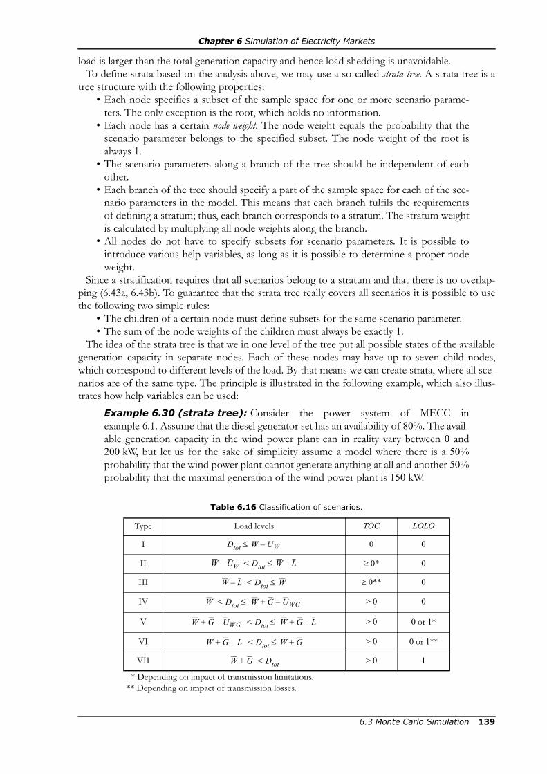
Chapter 6 Simulation of Electricity Markets
load is larger than the total generation capacity and hence load shedding is unavoidable.To define strata based on the analysis above, we may use a so-called strata tree. A strata tree is a
tree structure with the following properties:• Each node specifies a subset of the sample space for one or more scenario parame-
ters. The only exception is the root, which holds no information.• Each node has a certain node weight. The node weight equals the probability that the
scenario parameter belongs to the specified subset. The node weight of the root isalways 1.
• The scenario parameters along a branch of the tree should be independent of eachother.
• Each branch of the tree should specify a part of the sample space for each of the sce-nario parameters in the model. This means that each branch fulfils the requirementsof defining a stratum; thus, each branch corresponds to a stratum. The stratum weightis calculated by multiplying all node weights along the branch.
• All nodes do not have to specify subsets for scenario parameters. It is possible tointroduce various help variables, as long as it is possible to determine a proper nodeweight.
Since a stratification requires that all scenarios belong to a stratum and that there is no overlap-ping (6.43a, 6.43b). To guarantee that the strata tree really covers all scenarios it is possible to usethe following two simple rules:
• The children of a certain node must define subsets for the same scenario parameter.• The sum of the node weights of the children must always be exactly 1.
The idea of the strata tree is that we in one level of the tree put all possible states of the availablegeneration capacity in separate nodes. Each of these nodes may have up to seven child nodes,which correspond to different levels of the load. By that means we can create strata, where all sce-narios are of the same type. The principle is illustrated in the following example, which also illus-trates how help variables can be used:
Example 6.30 (strata tree): Consider the power system of MECC inexample 6.1. Assume that the diesel generator set has an availability of 80%. The avail-able generation capacity in the wind power plant can in reality vary between 0 and200 kW, but let us for the sake of simplicity assume a model where there is a 50%probability that the wind power plant cannot generate anything at all and another 50%probability that the maximal generation of the wind power plant is 150 kW.
Table 6.16 Classification of scenarios.
Type Load levels TOC LOLO
I Dtot ≤ 0 0
II < Dtot ≤ ≥ 0* 0
III < Dtot ≤ ≥ 0** 0
IV < Dtot ≤ > 0 0
V < Dtot ≤ > 0 0 or 1*
VI < Dtot ≤ > 0 0 or 1**
VII < Dtot > 0 1
* Depending on impact of transmission limitations.** Depending on impact of transmission losses.
W UW–
W UW– W L–
W L– W
W W G UWG–+
W G UWG–+ W G L–+
W G L–+ W G+
W G+
6.3 Monte Carlo Simulation 139

Chapter 6 Simulation of Electricity Markets
Lighting constitutes a large share of the load in the MECC system; hence, the powerdemand has a peak in the evening between 6 p.m. and 12 midnight. The load is thenN(175, 48)-distributed in Mji and N(75, 20)-distributed in Kijiji. During the rest of theday, the load in Kijiji is considerably lower—N(30, 7)-distributed—whereas there inMji also is some industrial activities resulting in a relatively high load during off-peakhours—the load is then N(120, 24)-distributed.a) Disregards of the transmission losses on the line between Mji and Kijiji. Suggestan appropriate strata tree for the system, and calculate the stratum weights.b) How will the strata tree change if the losses on the transmission line are included,if it can be assumed that the maximal losses are 3 kW?Solution: a) It would have been sufficient to create a strata tree with two levels belowthe root, if the probability distribution of both the available generation capacity andthe load had been the same regardless of the time of the day. To manage the load in asimple way, we can however introduce another level representing the time of the day.This is actually not a scenario parameter (i.e., time is not included in the multi-areamodel), but is an example of a help variable.We choose to place the time on the level just below the root, and on the next level weput the available generation capacity in the wind power plant and the diesel gen-erator set respectively. At the bottom level of the tree we have the load (D).31
As there are no transmission limitations and we disregard the transmission losses, wehave = 0, = 0 and = 0. We will therefore not find any scenarios of type II,III, V or VI in this strata tree. However, we will find a special case reminding of typeVII scenarios, but there TOC = 0, because = 0.
31. An alternative approach would have been to place the time below the available generation capacity. Theessential is that the time is above the load level of the tree, as the time determines which probability distri-bution should be used for calculation of the node weights on the load level.
00
Dtot
WG
≥ 0
ωh 0.075 0.0375 0.0375 0.3 0 0.15 0.15 0 0.025 0.0007 0.0243 0.05 0.05 0.0027 0.0971 0.0002
Type Spec. I Spec. IV VII I IV VII Spec. I Spec. IV VII I IV VIITOC 0 0 0 > 0 2 500 0 > 0 2 500 0 0 0 > 0 2 500 0 > 0 2 500
LOLO 1 0 1 0 1 0 0 1 1 0 1 0 1 0 0 1
0,1
1
Time Off-peak0.75
Figure 6.27 Strata tree for the system in example 6.30. All states of and Dtotare stated in kW.
W, G
1Root
≤ 150 > 150 ≤ 250 > 250 ≤ 150 150-400 > 400 ≥ 0 ≤ 150 > 150 ≤ 250 > 250 ≤ 150 150-400 > 400
2500
250150
0150
Peak
00
2500
250150
0150
0.25
0,1 0.4 0.4 0.1 0.1 0.4 0.4
0.5 0.5 1 0 0.5 0.5 0 1 0.027 0.973 0.5 0.5 0.027 0.971 0.002
W( )G( )
UW UWG L
G
140 6.3 Monte Carlo Simulation

Chapter 6 Simulation of Electricity Markets
We start by investigating the system during off-peak hours. As 75% of the time countsas off-peak, the node weight of the “off-peak” node is 0.75. There are now four possi-ble states of the available generation capacity; either the wind power plant is capableof generating 0 or 150 kW, while at the same time the diesel generator set may eitherbe available or unavailable. The probability of each these four states is easily calcu-lated, which gives us the node weights for the four first nodes on the generationcapacity level of the strata tree (see figure 6.27). In the first of these four nodes, there is no generation capacity available and loadshedding will therefore be necessary regardless of the current load. Thus, all these sce-narios have the same properties and there is no need for a further separation.In the next node we have 150 kW wind power available. In this case we need to childnodes: one for scenarios where the load does not exceed 150 kW and one for the sce-narios there the load is larger than 150 kW. According to theorem D.4 the total load inthe system is N(150, 25)-distributed, which means that the probability that the load isless than 150 kW is exactly 50%. The node weights of these two load nodes is there-fore 0.5 each. In the third node on the generation capacity level, only the diesel generator set is avail-able; therefore it is desirable to differentiate between scenarios where the total load islesser than or greater than 250 kW. However, when calculating the node weights, wefind that the probability that the total load does not exceed 250 kW is 99.997%. Con-sequently, the node weight of the other node (where Dtot > 250) is only 0.00003, whichmay cause numerical problems when generating random numbers. We may thereforechoose to exclude this node from the strata tree.Then we have a node where both the wind power plant and the diesel generator setcan be used for electricity generation. Here we need three load nodes to distinguishbetween scenarios with different properties. A load up to 150 kW can be coveredusing the wind power plant only, whereas both units are needed for a load between150 and 400 kW, and if the load exceeds 400 kW then load shedding is necessary. Thenode weight of the third load node is however in practice zero, and therefore weexclude this node. The two remaining load nodes will then each have the node weight0.5.If we study the system during peak hours, we will find the same states of the availablegeneration capacity. In the generation level, the right part of the strata tree is thereforeidentical to the left one. On the load level, it is the same intervals that are interesting,but as the total load during the evening is N(250, 52)-distributed, we will have othernode weights (see figure 6.27).Finally, the stratum weights are calculated by multiplying the node weights along eachbranch of the tree. The results are shown in figure 6.27.b) When considering the losses it is not always possible to predict the properties of ascenario just by comparing the available generation capacity and the total load. If forexample we investigate the last node on the generation level, we see that the availablegeneration capacity with negligible operation cost is 150 kW. As it is stated in theproblem that the losses will not exceed 3 kW, we can be certain that TOC = 0 andLOLO = 0 for all scenarios where the total load is less than 147 kW. When the totalload is between 147 and 150 kW, the losses will determine if the wind power plant issufficient or if the diesel generator set will be needed (which would result in TOC > 0).If the load is larger than 150 kW then the diesel generator set will definitely beneeded, i.e., we will have TOC > 0. The question is now if there will be a power deficit
6.3 Monte Carlo Simulation 141

Chapter 6 Simulation of Electricity Markets
or not. As long as the load plus the losses is not larger than the total generation capac-ity (400 kW) we will have LOLO = 0. We can be certain about this if the total load isbetween 150 and 397 kW. Between 397 and 400 kW, the losses will determine if we getLOLO = 0 or LOLO = 1. However, if the load exceeds 400 kW we can be certain thatload shedding will be necessary. Hence, we can identify five intervals for the load,where the scenarios will have similar properties, and these five intervals are repre-sented by five nodes in the strata tree, as illustrated in figure 6.28. A correspondingseparation will be necessary also for the other generation capacity nodes in the stratatree from figure 6.27.
As we can see in the example above, strata trees can become quite big even for a small powersystem. For larger electricity markets, we must expect that there will be thousands of possiblestates for the available generation capacity, resulting in a huge strata tree having ten thousands ofdifferent branches. Much of the gain from applying stratified sampling will be lost if there wouldbe so many strata. This problem can be managed by allowing one stratum to cover severalbranches of the strata tree. All scenarios of type I have the same characteristics; hence, all branchescorresponding to type I scenarios could be merged into a single stratum, etc. It should however benoted that this method means that conditional probability distributions have to be used. How tomanage these calculations is though beyond the scope of this presentation.
Sample Allocation
When strata have been defined, it is necessary to decide how many samples should be taken fromeach stratum. In general it is best to use the Neyman allocation, because it automatically allocatesmore samples to the strata where the uncertainty (i.e. the variance) is the largest, while strata witha large impact on the final result (i.e., high stratum weight) are prioritised. However, we are study-ing two—or maybe even more—result variables, while the Neyman allocation is based on compar-ing the variance in different strata for one single random variable. If the Neyman allocation is calcu-lated with regard to TOC and when compared to the Neyman allocation for LOLO, we will in mostcases get partly conflicting allocations. A simple solution to this dilemma is to simply use a com-promise between the allocations which are optimal for each variable.
To use the Neyman allocation it is necessary to have estimates of the variance within each stra-tum.32 To obtain such estimates we need to take a few samples from each stratum. Hence, at the
32. Cf. (6.48) and (6.49).
> 400
250150
≤ 147 147-150 150-397 397-400
Peak
Dtot
WG
Time
Type I III IV VI VIITOC 0 ≥ 0 > 0 > 0 2 500
LOLO 0 0 0 0 or 1 1
Figure 6.28 Part of the strata tree in example 6.30b.
142 6.3 Monte Carlo Simulation
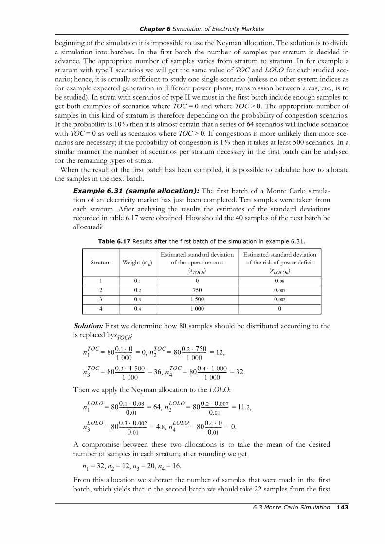
Chapter 6 Simulation of Electricity Markets
beginning of the simulation it is impossible to use the Neyman allocation. The solution is to dividea simulation into batches. In the first batch the number of samples per stratum is decided inadvance. The appropriate number of samples varies from stratum to stratum. In for example astratum with type I scenarios we will get the same value of TOC and LOLO for each studied sce-nario; hence, it is actually sufficient to study one single scenario (unless no other system indices asfor example expected generation in different power plants, transmission between areas, etc., is tobe studied). In strata with scenarios of type II we must in the first batch include enough samples toget both examples of scenarios where TOC = 0 and where TOC > 0. The appropriate number ofsamples in this kind of stratum is therefore depending on the probability of congestion scenarios.If the probability is 10% then it is almost certain that a series of 64 scenarios will include scenarioswith TOC = 0 as well as scenarios where TOC > 0. If congestions is more unlikely then more sce-narios are necessary; if the probability of congestion is 1% then it takes at least 500 scenarios. In asimilar manner the number of scenarios per stratum necessary in the first batch can be analysedfor the remaining types of strata.
When the result of the first batch has been compiled, it is possible to calculate how to allocatethe samples in the next batch.
Example 6.31 (sample allocation): The first batch of a Monte Carlo simula-tion of an electricity market has just been completed. Ten samples were taken fromeach stratum. After analysing the results the estimates of the standard deviationsrecorded in table 6.17 were obtained. How should the 40 samples of the next batch beallocated?
Solution: First we determine how 80 samples should be distributed according to theis replaced bysTOCh:
= = 0, = = 12,
= = 36, = = 32.
Then we apply the Neyman allocation to the LOLO:
= = 64, = = 11.2,
= = 4.8, = = 0.
A compromise between these two allocations is to take the mean of the desirednumber of samples in each stratum; after rounding we get
n1 = 32, n2 = 12, n3 = 20, n4 = 16.
From this allocation we subtract the number of samples that were made in the firstbatch, which yields that in the second batch we should take 22 samples from the first
Table 6.17 Results after the first batch of the simulation in example 6.31.
Stratum Weight (ωh)Estimated standard deviation
of the operation cost(sTOCh)
Estimated standard deviation of the risk of power deficit
(sLOLOh)
1 0.1 0 0.08
2 0.2 750 0.007
3 0.3 1 500 0.002
4 0.4 1 000 0
n1TOC 800.1 0⋅
1 000-------------- n2
TOC 800.2 750⋅1 000
--------------------
n3TOC 800.3 1 500⋅
1 000------------------------ n4
TOC 800.4 1 000⋅1 000
------------------------
n1LOLO 800.1 0.08⋅
0.01-------------------- n2
LOLO 800.2 0.007⋅0.01
----------------------
n3LOLO 800.3 0.002⋅
0.01---------------------- n4
LOLO 800.4 0⋅0.01
--------------
6.3 Monte Carlo Simulation 143

Chapter 6 Simulation of Electricity Markets
stratum, 2 from the second, 10 from the third and 6 from the fourth.When the second batch is finished it is possible to calculate a new Neyman allocation based on
the results of the first two batches. This procedure can be repeated after each batch, until an accu-rate enough result has been obtained.
A problem that might arise is that it might be detected that too many samples have been takenfrom a particular stratum. As the computation work of analysing these “unnecessary” samplesalready has been performed, it would be a waste of work to exclude these samples from the simu-lation. It is better to try to distribute the remaining samples as good as possible. We can say thatthose strata that have received too many samples have “stolen” samples from the remaining strata.The question is how the stolen samples should be divided between the strata; apparently there areseveral ways to solve this problem. An appropriate compromise is to reduce an equal share ofsamples from the affected strata. This can be done using the following algorithm:
Step 1. Determine the requested sample allocation for the b:th batch given by
= (6.51)
where denotes the number of samples in batch b from stratum h and is the total number of samples in stratum h according to the Neyman allocation.Step 2. Let H + be the index set of the strata which should be allocated more sam-ples and H – be the index set of those strata which have received too many samples,i.e.,
H + = {h: > 0}, H – = {h: < 0}. (6.52)
Step 3. Calculate the total number of requested samples according to
Δ+ (6.53)
and the total number of unnecessary samples according to
Δ– (6.54)
Step 4. The final sample allocation nh, b is obtained by choosing
nh, b = 0 ∀ h ∈ H – (6.55)
and
nh, b = (1 – Δ–/Δ+) ∀ h ∈ H +. (6.56)
The algorithm is illustrated in the following example:Example 6.32 (impossible sample allocation with several possiblecompromise solutions): The first batch of a Monte Carlo simulation of an elec-tricity market has just been completed. Ten samples were taken from each stratum.After analysing the results the estimates of the standard deviations recorded intable 6.18 were obtained. How should the 40 samples of the next batch be allocated?Solution: We start by examining the Neyman allocation of the operation cost:
= = 0, = = 8,
n'h b, nhNeyman nh c, ,
c 1=
b 1–
∑–
n'h b, nhNeyman
n'h b, n'h b,
n'h b,h H+
∈∑=
n'h b,h H–
∈∑–=
n'h b,
n1TOC 800.1 0⋅
1000-------------- n2
TOC 800.2 500⋅1000
--------------------
144 6.3 Monte Carlo Simulation

Chapter 6 Simulation of Electricity Markets
= = 38.4, = = 33.6.
Then we study the Neyman allocation according to the LOLO:
= = 64, = = 8.8,
= = 7.2, = = 0.
The compromise allocation after rounding isn1 = 32, n2 = 8, n3 = 23, n4 = 17.
As 10 samples have been taken from each stratum we receive the following requestedsample allocation in the second batch:
= 22, = –2, = 13, = 7.
The total number of unnecessary samples, Δ–, is thus 2 and the total number ofrequested samples, Δ+, is 42. The reduction in the strata which receive too few sampleis therefore 2/42 ≈ 5%. After rounding we get the following sample allocation for thesecond batch:
= 21, = 0, = 12, = 7.
EXERCISES6.1 The load in a certain power system is 100 MWh/h during workdays between 8 a.m.
and 8 p.m., 80 MWh/h during weekends between 8 a.m. and 8 p.m., 60 MWh/h dur-ing evenings between 8 p.m. and 12 p.m., and 50 MWh/h during all other periods.Draw the load duration curve.
6.2 Show that (6.17) and (6.18) yields the same expected generation.6.3 Prove equation (6.18).
Hint: A power plant g will be dispatched—provided that it is available—when theprevious plant is available but does not have enough capacity to cover the load, or ifthe previous power plant is unavailable. How can the expected generation in these twocases be calculated using equivalent load duration curves?
Table 6.18 Results after the first batch of the simulation in example 6.32.
Stratum Weight (ωh)Estimated standard deviation
of the operation cost(sTOCh)
Estimated standard deviation of the risk of power deficit
(sLOLOh)
1 0.1 0 0.08
2 0.2 500 0.0055
3 0.3 1 600 0.003
4 0.4 1 050 0
n3TOC 800.3 1600⋅
1000----------------------- n4
TOC 800.4 1050⋅1000
-----------------------
n1LOLO 800.1 0.08⋅
0.01-------------------- n2
LOLO 800.2 0.0055⋅0.01
-------------------------
n3LOLO 800.3 0.003⋅
0.01---------------------- n4
LOLO 800.4 0⋅0.01
--------------
n12 n2
2 n32 n4
2
n12 n2
2 n32 n4
2
Exercises 145
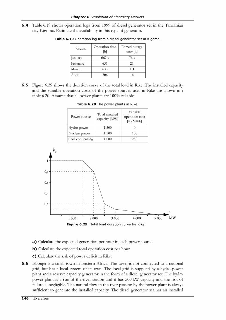
Chapter 6 Simulation of Electricity Markets
6.4 Table 6.19 shows operation logs from 1999 of diesel generator set in the Tanzaniancity Kigoma. Estimate the availability in this type of generator.
6.5 Figure 6.29 shows the duration curve of the total load in Rike. The installed capacityand the variable operation costs of the power sources uses in Rike are shown in itable 6.20. Assume that all power plants are 100% reliable.
a) Calculate the expected generation per hour in each power source.b) Calculate the expected total operation cost per hour.c) Calculate the risk of power deficit in Rike.
6.6 Ebbuga is a small town in Eastern Africa. The town is not connected to a nationalgrid, but has a local system of its own. The local grid is supplied by a hydro powerplant and a reserve capacity generator in the form of a diesel generator set. The hydropower plant is a run-of-the-river station and it has 500 kW capacity and the risk offailure is negligible. The natural flow in the river passing by the power plant is alwayssufficient to generate the installed capacity. The diesel generator set has an installed
Table 6.19 Operation log from a diesel generator set in Kigoma.
Month Operation time [h]
Forced outage time [h]
January 667.5 76.5February 651 21March 633 111April 706 14
Table 6.20 The power plants in Rike.
Power source Total installed capacity [MW]
Variable operation cost
[¤/MWh]
Hydro power 1 500 0Nuclear power 1 500 100Coal condensing 1 000 250
MW
x
5 000
F0
1
0,8
4 0003 0002 0001 000
0,6
0,2
0,4
Figure 6.29 Total load duration curve for Rike.
146 Exercises
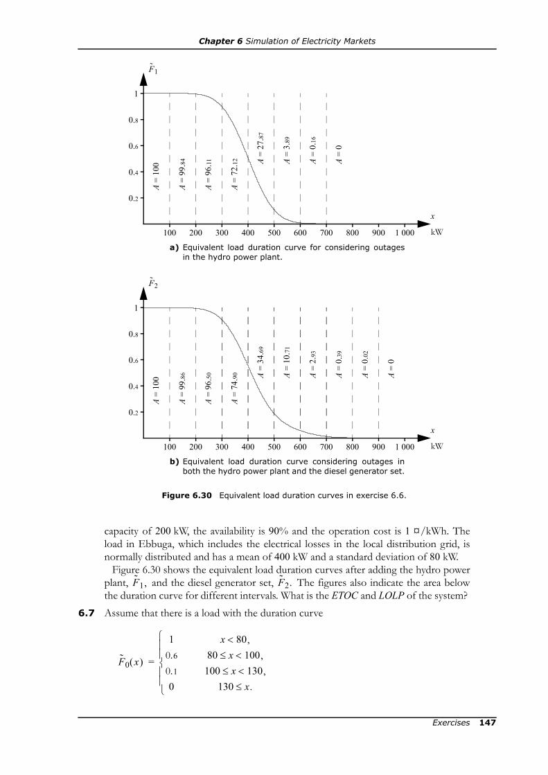
Chapter 6 Simulation of Electricity Markets
capacity of 200 kW, the availability is 90% and the operation cost is 1 ¤/kWh. Theload in Ebbuga, which includes the electrical losses in the local distribution grid, isnormally distributed and has a mean of 400 kW and a standard deviation of 80 kW.
Figure 6.30 shows the equivalent load duration curves after adding the hydro powerplant, and the diesel generator set, The figures also indicate the area belowthe duration curve for different intervals. What is the ETOC and LOLP of the system?
6.7 Assume that there is a load with the duration curve
F1
kW
x
1 000
1
0.6
0.4
0.2
0.8
900800700600500400300200100
Figure 6.30 Equivalent load duration curves in exercise 6.6.
A =
100
A =
99.84
A =
96.11
A =
72.12 A
= 27
.87
A =
3.89
A =
0.16
A =
0
A =
100
A =
99.86
A =
96.50
A =
74.90 A
= 34
.69
A =
10.71
A =
2.93
A =
0.39
A =
0.02
A =
0
F2
kW
x
1 000900800700600500400300200100
a) Equivalent load duration curve for considering outagesin the hydro power plant.
b) Equivalent load duration curve considering outages inboth the hydro power plant and the diesel generator set.
1
0.6
0.4
0.2
0.8
F1, F2.
F0 x( )
10.60.10⎩
⎪⎪⎨⎪⎪⎧
=
x 80,<80 x 100,<≤
100 x 130,<≤130 x.≤
Exercises 147

Chapter 6 Simulation of Electricity Markets
a) Calculate LOLP and EENS if the system is supplied by a 120 MW unit, which isalways available.b) Calculate LOLP and EENS if the system is supplied by a 150 MW unit, which has90% availability.
6.8 Large parts of the rural areas of Eggwanga have no access to electricity. To speed upthe development, the Eggwangan authorities have decided to let private companiesbuild and operate isolated power systems in rural areas. The condition is that the com-panies do not charge more than 1 ¤/kWh and that the risk of power deficit does notexceed 2%. In the small town Akabuga some local businessmen are considering tostart the Akabuga Electricity Company Ltd. (AECL), which will build a local gridwhich can supply the town and its closes surroundings with electric power. Oneoption is to supply the grid from diesel generator sets. It is planned to use a numberof similar diesel generator sets, where each unit has a capacity of 200 kW, availability90% and a generation cost of 0.50 ¤/kWh. The investment and maintenance costs ofa diesel generator set is 50 000 ¤/year. The investment and maintenance costs of thedistribution system is expected to be 2 M¤/year.a) The equivalent load duration curve when four diesel generator sets is shown intable 6.21. Will AECL be profitable according to this calculation? (Disregard theLOLP requirement in this assignment.)b) Would it be profitable to invest in another diesel generator set, so that the totalinstalled capacity is 1 000 kW? (Continue to disregard the LOLP requirement.)
6.9 Another option for the electricity supply of Akabuga is to use diesel generator sets ofthe same sort as in exercise 6.8, as well as a small hydro power plant in Ekikko, whichis located a short distance from the town. The hydro power plant has an installedcapacity of 400 kW. Both operation cost and the risk of failures in the hydro powerplant is negligible.a) Figure 6.31 shows the load duration curve, as well as the equivalent load dura-
Table 6.21 Equivalent load duration curves in exercise 6.8.
Interval
1 1 1 1 1 x < 4000.6 0.64 0.676 0.7084 0.73756 400 ≤ x < 6000.1 0.15 0.199 0.2467 0.29287 600 ≤ x < 8000.01 0.019 0.0321 0.04879 0.068581 800 ≤ x < 1 000
0 0.001 0.0028 0.00573 0.010036 1 000 ≤ x < 1 2000 0 0.0001 0.00037 0.000906 1 200 ≤ x < 1 4000 0 0 0.00001 0.000046 1 400 ≤ x < 1 6000 0 0 0 0.000001 1 600 ≤ x < 1 8000 0 0 0 0 1 800 ≤ x
Table 6.22 Integral calculations of the equivalent load duration curve in exercise 6.9
g = 1 200.00 199.66 119.11 21.17 1.73 0.01
g = 4 200.00 199.75 140.94 49.97 9.82 1.19
F0 x( ) F1 x( ) F2 x( ) F3 x( ) F4 x( )
Fg x( ) xd0
200
∫ Fg x( ) xd200
400
∫ Fg x( ) xd400
600
∫ Fg x( ) xd600
800
∫ Fg x( ) xd800
1 000
∫ Fg x( ) xd1 000
∞
∫
F0,
148 Exercises
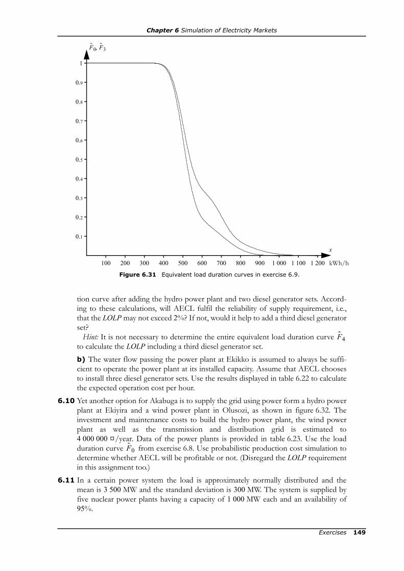
Chapter 6 Simulation of Electricity Markets
tion curve after adding the hydro power plant and two diesel generator sets. Accord-ing to these calculations, will AECL fulfil the reliability of supply requirement, i.e.,that the LOLP may not exceed 2%? If not, would it help to add a third diesel generatorset?
Hint: It is not necessary to determine the entire equivalent load duration curve to calculate the LOLP including a third diesel generator set.b) The water flow passing the power plant at Ekikko is assumed to always be suffi-cient to operate the power plant at its installed capacity. Assume that AECL choosesto install three diesel generator sets. Use the results displayed in table 6.22 to calculatethe expected operation cost per hour.
6.10 Yet another option for Akabuga is to supply the grid using power form a hydro powerplant at Ekiyira and a wind power plant in Olusozi, as shown in figure 6.32. Theinvestment and maintenance costs to build the hydro power plant, the wind powerplant as well as the transmission and distribution grid is estimated to4 000 000 ¤/year. Data of the power plants is provided in table 6.23. Use the loadduration curve from exercise 6.8. Use probabilistic production cost simulation todetermine whether AECL will be profitable or not. (Disregard the LOLP requirementin this assignment too.)
6.11 In a certain power system the load is approximately normally distributed and themean is 3 500 MW and the standard deviation is 300 MW. The system is supplied byfive nuclear power plants having a capacity of 1 000 MW each and an availability of95%.
F4
300 kWh/h
x
F0 F3,
100 200 400 500 600 700 800 900 1 000 1 100 1 200
Figure 6.31 Equivalent load duration curves in exercise 6.9.
1
0.6
0.8
0.9
0.7
0.5
0.1
0.3
0.4
0.2
F0
Exercises 149

Chapter 6 Simulation of Electricity Markets
a) Use the normal approximation to determine the system LOLP. The distributionfunction of the standardised normal distribution is found in appendix D.b) Assume that V MW of wind power is added to this system and that the outage inthese power plants can be assumed to be normally distributed with the mean
= 0,6V and the standard deviation = 0.1V. Use the normal approximation ofprobabilistic production cost simulation to determine how much wind power is neces-sary to replace one of the nuclear power plants, without changing the system LOLPcompared to part a.
6.12 Assume that an electricity market has been simulated using Monte Carlo techniquesand that the following results have been obtained:
= 512 000 ¤/h, = 16,
where toci and loloi are the observations from scenario i of TOC and LOLO respec-tively. Which estimates of ETOC and LOLP are obtained from this simulation?
6.13 In a Monte Carlo simulation of an multi-area model, 10 000 scenarios have been gen-erated. In 12 of these, the total unserved power, ΣUn, was larger than zero. What is theLOLP estimate from this simulation?
6.14 Consider the suggested power system for Akabuga in exercise 6.8. Generate a sce-nario for a Monte Carlo simulation of the power system of Akabuga using the follow-ing random numbers from a U(0, 1)-distribution: 0.93 and 0.74. Use the durationcurves of load as well as available generation capacity found in figure 6.33. Also gener-ate the complementary scenarios. Which estimations of ETOC and LOLP are obtainedfrom the four scenarios?
Akabuga
Ekiyira
Olusozi
Figure 6.32 Suggested power system for Akabuga in exercise 6.10.
Table 6.23 Data of the planned power plants in exercise 6.10.
Power plant Installed capacity [kW]
Generation cost [¤/kWh]
Possible states of the available generation capacity
Ekiyira 800 Negligible 800 kW (100%)
Olusozi 600 Negligible 600 kW (12%), 400 kW (18%),200 kW (37%), 0 kW (33%)
μOv σOv
tocii 1=
2 000
∑ loloii 1=
2 000
∑
150 Exercises
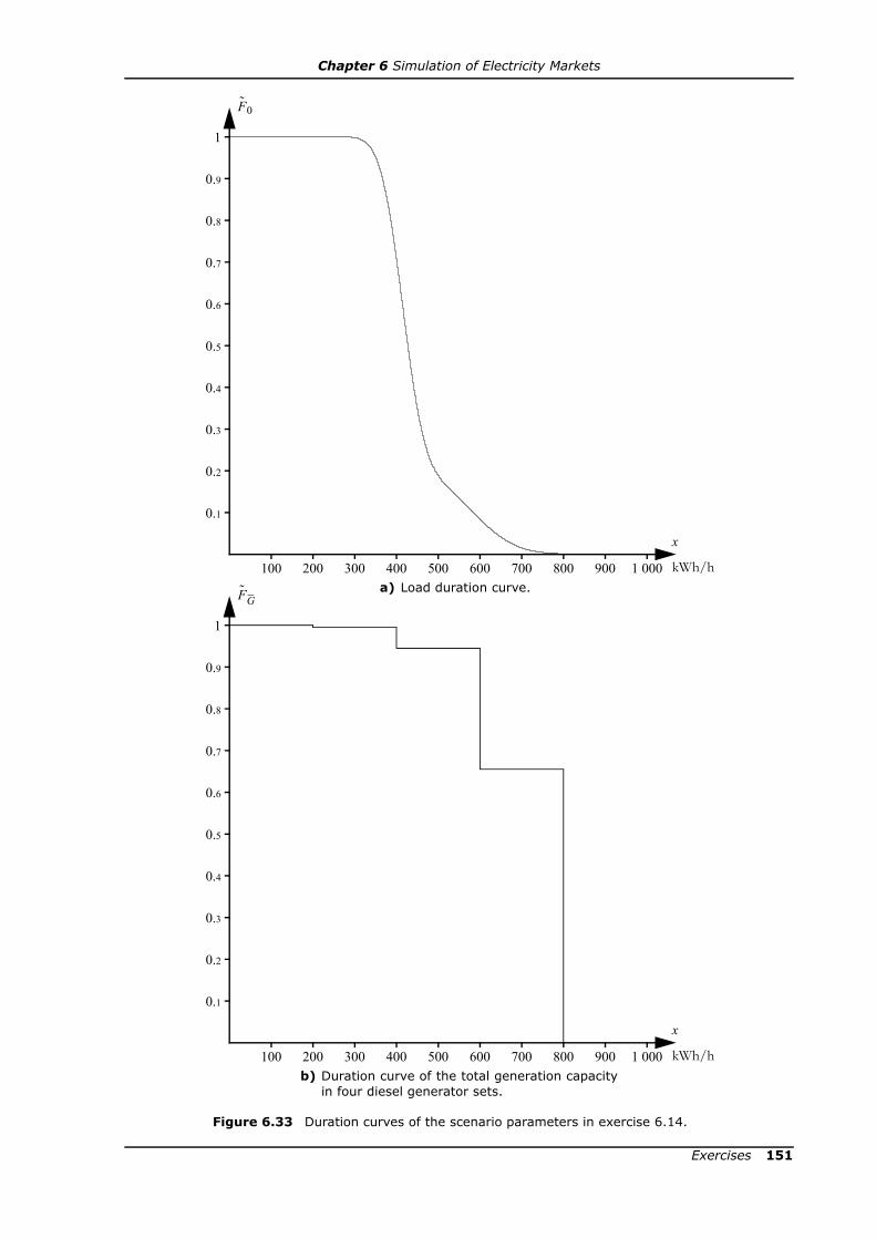
Chapter 6 Simulation of Electricity Markets
400 kWh/h
x
100 600 800
F0
1 000300 500 900200 700
400100 600
1
0.6
800
0.8
FG
1 000
0.9
0.7
300 500 900200 700 kWh/h
x
a) Load duration curve.
b) Duration curve of the total generation capacityin four diesel generator sets.
Figure 6.33 Duration curves of the scenario parameters in exercise 6.14.
0.5
0.1
0.3
0.4
0.2
1
0.6
0.8
0.9
0.7
0.5
0.1
0.3
0.4
0.2
Exercises 151

Chapter 6 Simulation of Electricity Markets
6.15 Consider the suggested power system for Akabuga in exercise 6.9.b. The losses on theline between Ekikko and Akabuga can be modelled as a quadratic function,L(P) = 2·10–5P2. The following five scenarios have been generated in a Monte Carlosimulation of this system:
Which estimate of ETOC is obtained from these five scenarios if a control variate isused?
6.16 Consider the suggested power system for Akabuga in exercise 6.10. In a closer studyof the suggested option, AECL has developed a more detailed model of the system,where for example the transmission losses are included. The losses between Ekiyiraand Olusozi are modelled as a quadratic function, L1, 2(P1, 2) = 3·10–5 and thelosses on the line between Olusozi and Akabuga are assumed to be L2, 3(P2, 3) =8·10–5·
To make sure that the estimate of the risk of power deficit is accurate, it is recom-mended to use stratified sampling.a) Figure 6.34 shows a part of the strata tree in this simulation. (The strata tree is verylarge—2 726 branches—and therefore just a small part is shown.) Suggest appropri-ate intervals for the nodes representing the load.b) If each branch of the strata tree is treated as a separate stratum, there would be2 726 strata. This is somewhat unnecessary; therefore, all strata of the same type hasbeen merged together. Only three strata remain after the merging.
Three result variables are interesting in this simulation: LOLO (power deficit), H(hydro power generation) and W (wind power generation). After some simulation theresults shown in tabell 6.24 have been collected. Which estimates do we get of the riskof power deficit and the generation in the power plants?
6.17 The first batch of a Monte Carlo simulation of an electricity market has just beencompleted. 16 samples were taken from each stratum. After analysing the results the
[kW] [kW] [kW] [kW] D
400 200 200 0 724400 200 200 200 503400 200 0 200 381400 200 200 200 612400 200 200 200 449
H G1 G2 G3
P1 2,2 ,
P2 3,2 .
Root
H 800=W 350=
= available capacity in the hydro power plant = available capacity in the wind power plant
HW
? < D? < D ≤ ?D ≤ ?
Figure 6.34 Part of the strata tree in exercise 6.16.
152 Exercises
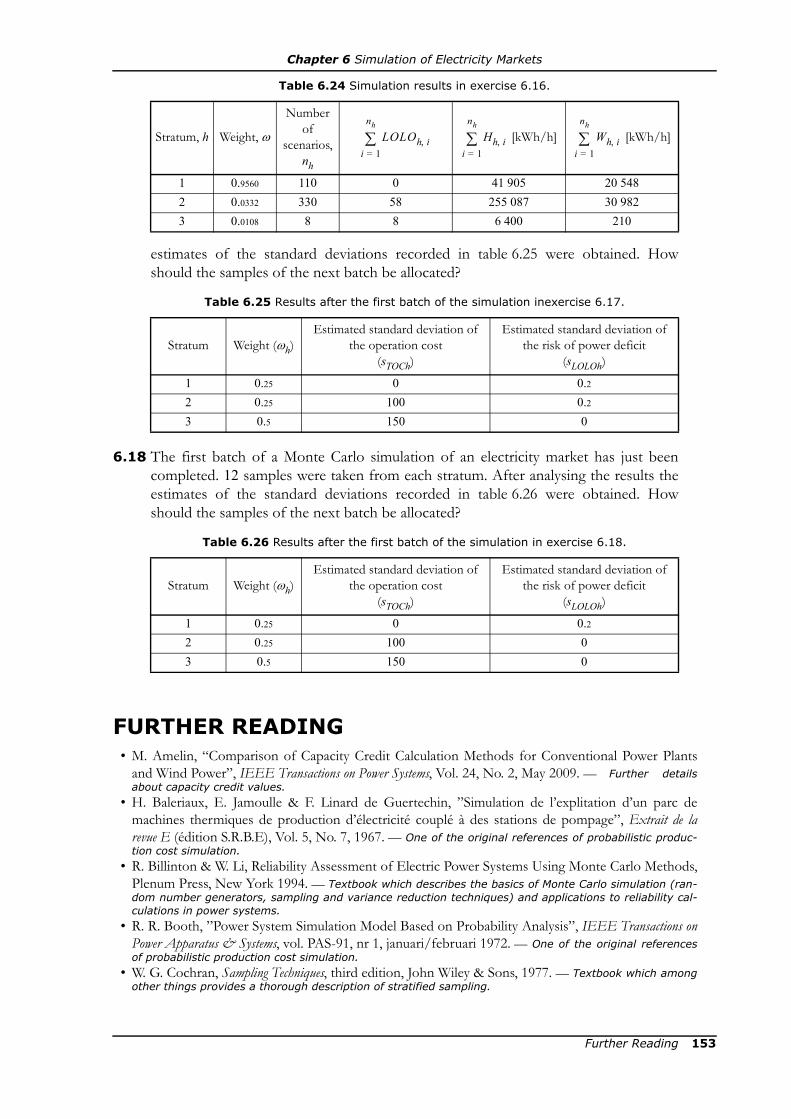
Chapter 6 Simulation of Electricity Markets
estimates of the standard deviations recorded in table 6.25 were obtained. Howshould the samples of the next batch be allocated?
6.18 The first batch of a Monte Carlo simulation of an electricity market has just beencompleted. 12 samples were taken from each stratum. After analysing the results theestimates of the standard deviations recorded in table 6.26 were obtained. Howshould the samples of the next batch be allocated?
FURTHER READING• M. Amelin, “Comparison of Capacity Credit Calculation Methods for Conventional Power Plants
and Wind Power”, IEEE Transactions on Power Systems, Vol. 24, No. 2, May 2009. — Further detailsabout capacity credit values.
• H. Baleriaux, E. Jamoulle & F. Linard de Guertechin, ”Simulation de l’explitation d’un parc demachines thermiques de production d’électricité couplé à des stations de pompage”, Extrait de larevue E (édition S.R.B.E), Vol. 5, No. 7, 1967. — One of the original references of probabilistic produc-tion cost simulation.
• R. Billinton & W. Li, Reliability Assessment of Electric Power Systems Using Monte Carlo Methods,Plenum Press, New York 1994. — Textbook which describes the basics of Monte Carlo simulation (ran-dom number generators, sampling and variance reduction techniques) and applications to reliability cal-culations in power systems.
• R. R. Booth, ”Power System Simulation Model Based on Probability Analysis”, IEEE Transactions onPower Apparatus & Systems, vol. PAS-91, nr 1, januari/februari 1972. — One of the original referencesof probabilistic production cost simulation.
• W. G. Cochran, Sampling Techniques, third edition, John Wiley & Sons, 1977. — Textbook which amongother things provides a thorough description of stratified sampling.
Table 6.24 Simulation results in exercise 6.16.
Stratum, h Weight, ω
Number of
scenarios, nh
[kWh/h] [kWh/h]
1 0.9560 110 0 41 905 20 5482 0.0332 330 58 255 087 30 9823 0.0108 8 8 6 400 210
Table 6.25 Results after the first batch of the simulation inexercise 6.17.
Stratum Weight (ωh)Estimated standard deviation of
the operation cost(sTOCh)
Estimated standard deviation of the risk of power deficit
(sLOLOh)
1 0.25 0 0.22 0.25 100 0.23 0.5 150 0
Table 6.26 Results after the first batch of the simulation in exercise 6.18.
Stratum Weight (ωh)Estimated standard deviation of
the operation cost(sTOCh)
Estimated standard deviation of the risk of power deficit
(sLOLOh)
1 0.25 0 0.22 0.25 100 03 0.5 150 0
LOLOh i,i 1=
nh
∑ Hh i,i 1=
nh
∑ Wh i,i 1=
nh
∑
Further Reading 153

154
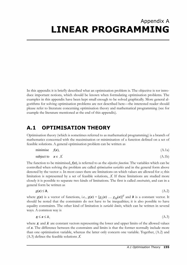
Appendix A
LINEAR PROGRAMMING
In this appendix it is briefly described what an optimisation problem is. The objective is tor intro-duce important notions, which should be known when formulating optimisation problems. Theexamples in this appendix have been kept small enough to be solved graphically. More general al-gorithms for solving optimisation problems are not described here—the interested reader shouldplease refer to literature concerning optimisation theory and mathematical programming (see forexample the literature mentioned at the end of this appendix).
A.1 OPTIMISATION THEORYOptimisation theory (which is sometimes referred to as mathematical programming) is a branch ofmathematics concerned with the maximisation or minimisation of a function defined on a set offeasible solutions. A general optimisation problem can be written as
minimise f(x), (A.1a)
subject to x ∈ X. (A.1b)
The function to be minimised, f(x), is referred to as the objective function. The variables which can becontrolled when solving the problem are called optimisation variables and in the general form abovedenoted by the vector x. In most cases there are limitations on which values are allowed for x; thislimitation is represented by a set of feasible solutions, X. If these limitations are studied moreclosely it is possible to separate two kinds of limitations. The first is called constraints, and can in ageneral form be written as
g(x) ≤ b, (A.2)where g(x) is a vector of functions, i.e., g(x) = [g1(x) … gM(x)]T and b is a constant vector. Itshould be noted that the constraints do not have to be inequalities; it is also possible to haveequality constraints. The other kind of limitation is variable limits, which can be written in severalways. A common way is
(A.3)
where and are constant vectors representing the lower and upper limits of the allowed valuesof x. The difference between the constraints and limits is that the former normally include morethan one optimisation variable, whereas the latter only concern one variable. Together, (A.2) and(A.3) defines the feasible solutions X.
x x x,≤ ≤
x x
A.1 Optimisation Theory 155

Appendix A Linear Programming
Linear Programming
A linear programming problem (LP problem) is a special class of optimisation problem, where theobjective function as well as the constraints are linear functions. An LP problem in standard formhaving N constraints and M variables is formulated as follows:
minimise c1x1 + c2x2 + … + cMxM (A.4)
subject to a1, 1x1 + a1, 2x2 + … + a1, MxM = b1,
a2, 1x1 + a2, 2x2 + … + a2, MxM = b2,
…
aN, 1x1 + aN, 2x2 + … + aN, MxM = bN,
xi ≥ 0, i = 1, …, M.
This problem can be formulated in a more compact manner using matrices:
minimise cTx (A.5)
subject to Ax = b, (A.5a)
x ≥ 0, (A.5b)
where
c = x = A = b =
An advantage of using linear programming is that there is commercial software available, whichcan provide fast solutions to problems having thousands or tens of thousands optimisation varia-bles.
Formulating Optimisation Problems
When formulating optimisation problem is very important to be clear. Even relatively simpleproblems may require a large number of variables and parameters; hence, misunderstandings easilyoccur if the problem is not formulated so that it is easy to read and understand. What is easy toread and understand is of course depending on the context. A mathematician, who wants to ana-lyse how the problem should be solved, will probably prefer to have the problem formulated insome kind of standard form, which often includes a very compact formulation using vectors, ma-trices, etc. (cf. the previous section).
This strict mathematical form is however not very practical for engineering purposes, when it ismore interesting to see the coupling between the real problem and its mathematical formulation. Itis for example impractical to collect all optimisation variables in a vector x; it is preferable choosesuch symbols for the optimisation variables so that it is possible to immediately realise whichquantity they denote. For the same reason it is impractical to use a vector function to describe theconstraints; it is better to write each constraint separately. If the problem includes several similarconstraints then it is possible to avoid repeating all these constraints by introducing appropriateindices for the concerned variables and parameters. In this compendium, we will stick to this wayof formulating optimisation problems.
Even though a problem is formulated in a less strict mathematical form it is recommended to tryto keep the structure of the optimisation problem, i.e., it should be easy to see what is the objec-
c1
cM
,…
x1
xM
,…
a1 1, … a1 M,
aN 1, … aN M,
,… ……
b1
bN
.…
156 A.1 Optimisation Theory

Appendix A Linear Programming
tive function, which are the constraints and which are the variable limits. It is also important toclearly state which symbols denote optimisation variables and which denote problem parameters.An appropriate routine when formulating optimisation problems is therefore as follows:
•Formulate the problem in words. Start by thinking through the problem youare about to formulate and make sure that you understand it. Then describe yourproblem in words.
•Define symbols. Review which variables and parameters which are involved in theproblem and state clear definitions of them. If you are using indices to distinguishsimilar variables it is recommended to already at this point state the possible values foreach index and each variable.
•Write the mathematical formulation. Formulating the problem can now beconsidered as the problem of translating the problem formulated in words into equa-tions and inequalities using the defined notation.
A.2 EXAMPLES OF LP PROBLEMSWe start by an example of how an LP problem is formulated in standard form:
Example A.1 (LP problem in standard form): Alice’s mother will have someguests and wants to serve coffee and something light to eat. The mother says ”Alice,can you please go to the shop? I would like to fill the fruit bowl (which can containtwo litres) and my five guests should have at least two each of what you buy. Here is100 SEK. You can keep the change.”Alice thinks that apples and pears will be nice. The pears cost 3 SEK each and apples5 SEK each. It can be assumed that there are 6 pears to 1 litre; the apples are largerand have a volume of 0.3 litres each. Formulate Alice’s planning problem as an LPproblem in standard form.Solution: Let x1 denote the number of pears and x2 the number of apples Alice isbuying. The problem can be formulated Alice minimising the costs of the purchasewile fulfilling the requirements of her mother:
minimise z = 3x1 + 5x2
subject to x1 + 0.3x2 ≥ 2,
x1 + x2 ≥ 10,
x1 ≥ 0, x2 ≥ 0.
The solution to this problem is shown in figure A.1. The borders of the constraintsand the variable limits are marked by dashed lines and the area which does not fulfilthe requirements is shaded. Different combinations of x1 and x2 which result in thesame value of the objective function are shown by thin, straight lines. As can be seenin the figure, the minimal value of z is obtained in the intersection of the constraintsx1/6 + 0.3x2 ≥ 2 and 4x1 + x2 ≥ 10. In that point we have x1 = 7.5 and x2 = 2.5, i.e., Aliceshould by 7.5 pears and 2.5 apples.To write Alice’s problem in standard form we must introduce slack variables, to obtainequality constraints. Hence, we get the following constraints:
x1 + 0.3x2 – x3 = 2,
16---
16---
A.2 Examples of LP problems 157
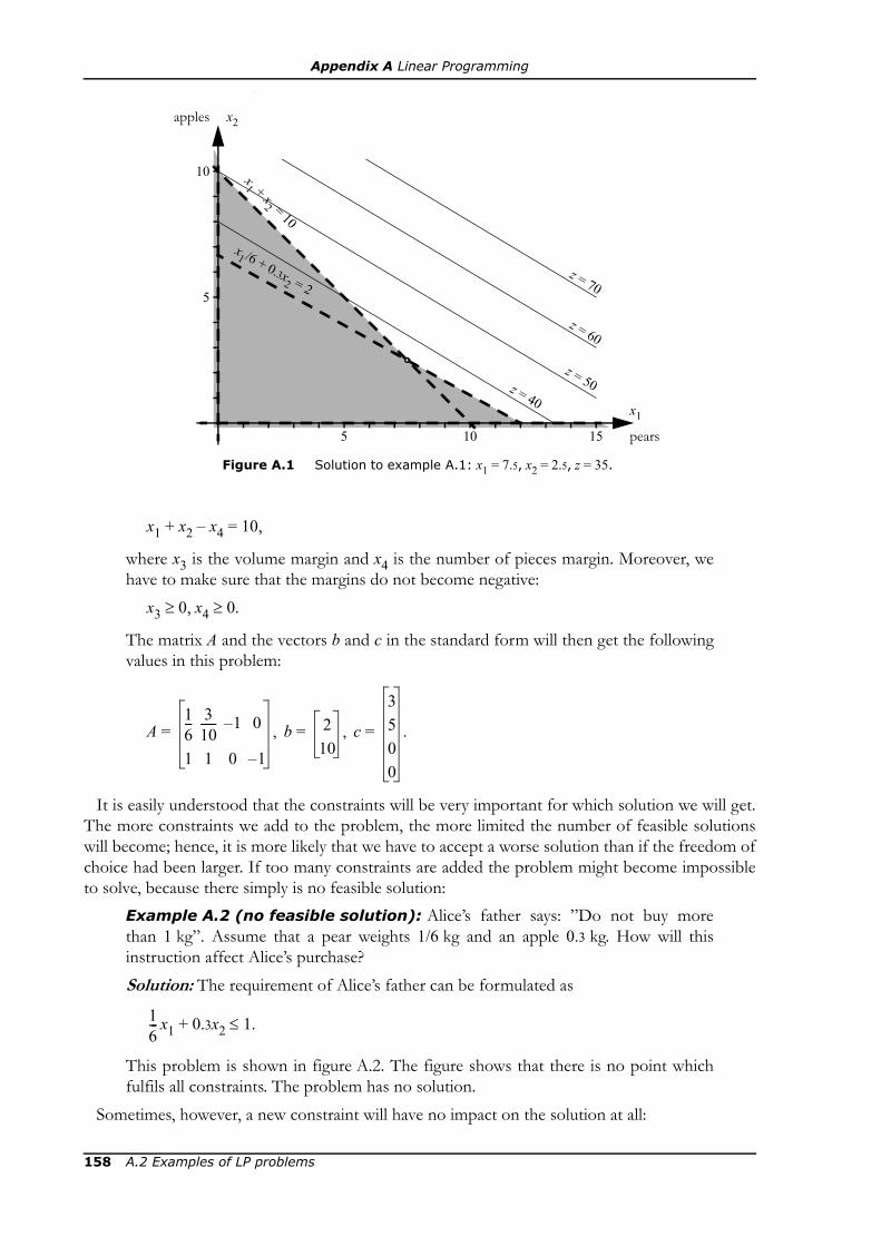
Appendix A Linear Programming
x1 + x2 – x4 = 10,
where x3 is the volume margin and x4 is the number of pieces margin. Moreover, wehave to make sure that the margins do not become negative:
x3 ≥ 0, x4 ≥ 0.
The matrix A and the vectors b and c in the standard form will then get the followingvalues in this problem:
A = b = c =
It is easily understood that the constraints will be very important for which solution we will get.The more constraints we add to the problem, the more limited the number of feasible solutionswill become; hence, it is more likely that we have to accept a worse solution than if the freedom ofchoice had been larger. If too many constraints are added the problem might become impossibleto solve, because there simply is no feasible solution:
Example A.2 (no feasible solution): Alice’s father says: ”Do not buy morethan 1 kg”. Assume that a pear weights 1/6 kg and an apple 0.3 kg. How will thisinstruction affect Alice’s purchase?Solution: The requirement of Alice’s father can be formulated as
x1 + 0.3x2 ≤ 1.
This problem is shown in figure A.2. The figure shows that there is no point whichfulfils all constraints. The problem has no solution.
Sometimes, however, a new constraint will have no impact on the solution at all:
Figure A.1 Solution to example A.1: x1 = 7.5, x2 = 2.5, z = 35.
5 pears
x1
5
apples x2
10 15
10
z = 70
x1 + x
2 = 10
x1 /6 + 0.3x2 = 2
z = 60
z = 50z = 40
16--- 3
10------ 1– 0
1 1 0 1–, 2
10,
3500
.
16---
158 A.2 Examples of LP problems
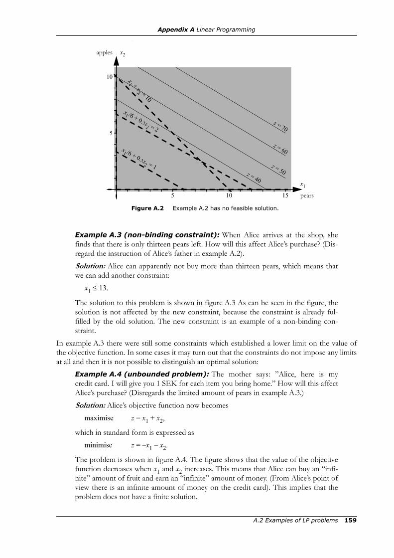
Appendix A Linear Programming
Example A.3 (non-binding constraint): When Alice arrives at the shop, shefinds that there is only thirteen pears left. How will this affect Alice’s purchase? (Dis-regard the instruction of Alice’s father in example A.2).Solution: Alice can apparently not buy more than thirteen pears, which means thatwe can add another constraint:
x1 ≤ 13.
The solution to this problem is shown in figure A.3 As can be seen in the figure, thesolution is not affected by the new constraint, because the constraint is already ful-filled by the old solution. The new constraint is an example of a non-binding con-straint.
In example A.3 there were still some constraints which established a lower limit on the value ofthe objective function. In some cases it may turn out that the constraints do not impose any limitsat all and then it is not possible to distinguish an optimal solution:
Example A.4 (unbounded problem): The mother says: ”Alice, here is mycredit card. I will give you 1 SEK for each item you bring home.” How will this affectAlice’s purchase? (Disregards the limited amount of pears in example A.3.)Solution: Alice’s objective function now becomes
maximise z = x1 + x2,
which in standard form is expressed asminimise z = –x1 – x2.
The problem is shown in figure A.4. The figure shows that the value of the objectivefunction decreases when x1 and x2 increases. This means that Alice can buy an “infi-nite” amount of fruit and earn an “infinite” amount of money. (From Alice’s point ofview there is an infinite amount of money on the credit card). This implies that theproblem does not have a finite solution.
5 pears
x1
5
apples x2
10 15
10
z = 70
x1 + x
2 = 10
x1 /6 + 0.3x2 = 2
z = 60
z = 50
Figure A.2 Example A.2 has no feasible solution.
x1 /6 + 0.3x2 = 1z = 40
A.2 Examples of LP problems 159

Appendix A Linear Programming
An interesting property of LP problems is that a small change in the objective function does notaffect the optimal solution, but only the value of the objective function, as shown in the followingexample:
Example A.5 (new objective function): When Alice arrives at the shop shefinds that pears cost 4 SEK each. How will this affect Alice’s purchase?Solution: The objective function now becomes
minimise z = 4x1 + 5x2
Figure A.3 Solution to example A.3: x1 = 7.5, x2 = 7.5, z = 35.
5 pears
x1
5
apples x2
10 15
10
z = 70
x1 + x
2 = 10
x1 /6 + 0.3x2 = 2
z = 40
z = 60
z = 50
Figure A.4 Solution to example A.4: x1 = ∞, x2 = ∞, z = –∞.
5 pears
x1
5
apples x2
10 15
10 x1 + x
2 = 10
x1 /6 + 0.3x2 = 2
z = –12
z = –14
z = –16
z = –18
z = –20
z = –22
z = –24
160 A.2 Examples of LP problems

Appendix A Linear Programming
and the new problem is shown in figure A.5. As can be seen in the figure, the samepoint is optimal—Alice should still buy 7.5 pears and 2.5 apples, but the total cost isnow 42.50 SEK.
In some cases there are several solutions which are equally good. This means that there in thesecases are an finite optimal value of the objective function, but there is an infinite number of solu-tions.
Example A.6 (degenerated solution): Assume that Alice finds that the pearscost 5 SEK each. How will this affect Alice’s purchase?Solution: The objective function now becomes
minimise z = 4x1 + 5x2,
which is shown in figure A.6. In this case there is no unique solution, but an infinitenumber of solutions all providing the optimal value z = 50.
Some problems have several different solutions which all give a value of the objective functionwhich is close to the optimal—it is said that these problems have a flat optimum. A flat optimumindicates that the problem is almost degenerated. In practice a flat optimum means that a somedeviations from the optimal solution might be tolerable, as the impact on the objective function issmall.
Example A.7 (flat optimum): Compare the following two cases:a) Pears cost 4.90 SEK each and apples 5 SEK each,b) Pears cost 5 SEK each and apples cost 4,90 SEK each.
Solution: The objective function in case a isminimise z = 4.9x1 + 5x2,
and in case b we getminimise z = 5x1 + 4.9x2.
Figure A.5 Solution to example A.5: x1 = 7.5, x2 = 2.5, z = 42.5.
5 pears
x1
5
apples x2
10 15
10 x1 + x
2 = 10
x1 /6 + 0.3x2 = 2
z = 40z = 50
z = 60
z = 70
A.2 Examples of LP problems 161

Appendix A Linear Programming
Both solutions are displayed in figure A.7. As can be seen in the figure, we get twovery different solutions, but the optimal value of the objective function is approxi-mately the same in both cases. Also notice that in both cases the value of the objectivefunction would not deteriorate very much if we choose the wrong alternative. In casea it is optimal to buy 7.5 pears and 2.5 apples (cost 49.25 SEK), but if Alice would buyonly apples instead, the cost would just increase by 0.75 SEK. Also in case b the costwould only increase by 0.75 SEK if she buys 7.5 pears and 2.5 apples instead of buyingjust apples.
Each LP problem has a corresponding so-called dual problem. Analysis of the dual problem canprovide useful information about the original (the primal) problem. A more thorough explanationof the relation between primal and dual problems would be too complex for this appendix, but inthe following two examples we will show how to obtain the dual problem and how the solutioncan be utilised.
Example A.8 (dual formulation of an LP problem): When Alice is passingby the candy in the shop, she recalls that her mother din not say anything about buy-ing fruit. Alice could buy popcorn and bonbons instead, but would that be cheaper?Assume that popcorn cost λ1 SEK/litre and the bonbons cost λ2 SEK each. Moreo-ver, assume that the volume of the bonbons is negligible and that the number of pop-corn is not considered. Let x5 be the number of litres of popcorn and x6 the numberof bonbons. Which is the maximal prices of popcorn and bonbons which Alice canafford if she does not want to loose money on this alternative?Solution: With these new conditions, Alice’s problem can be written as
Φ(λ1, λ2) = minimise 3x1 + 5x2 + λ1x5 + λ2x6
subject to x1 + 0.3x2 – x3 + x5 = 2,
x1 + x2 – x4 + x6 = 10,
Figure A.6 Solution to example A.6: x1 ∈ [0, 7.5], x2 = 10 – x1, z = 50.
5 pears
x1
5
apples x2
10 15
10 x1 + x
2 = 10
x1 /6 + 0.3x2 = 2
z = 40z = 50
z = 70z = 60
16---
162 A.2 Examples of LP problems

Appendix A Linear Programming
xi ≥ 0, i = 1, …, 6,
where the prices λ1 and λ2 both must be larger than or equal to zero. If we rearrangethe constraints to obtain expressions for x5 and x6, and substitute these expressionsinto the objective function, then the problem becomes
Φ(λ1, λ2) = minimise +
+ λ2(10 – x1 – x2 – x4)subject to xi ≥ 0, i = 1, …, 4.
Figure A.7 Solutions to example A.7.
5 pears
x1
5
apples x2
10 15
10 x1 + x
2 = 10
x1 /6 + 0.3x2 = 2
5 pears
x1
5
apples x2
10 15
10 x1 + x
2 = 10
x1 /6 + 0.3x2 = 2
a) x1 = 7.5, x2 = 2.5, z = 49.25.
z = 40
z = 50z = 70
z = 60z = 40
z = 50z = 70
z = 60
b) x1 = 0, x2 = 10, z = 49.
3x1 5x2 λ1 2 16---x1– 0.3x2– x3–⎝ ⎠
⎛ ⎞+ +
A.2 Examples of LP problems 163

Appendix A Linear Programming
This means that we have applied Lagrange relaxation to the constraints inexample A.1. This has resulted in two new variables: λ1 and λ2. λ1 is a dual variableconnected to the first constraint (because the first constraint is a volume constraintand popcorn are assumed to only possess volume). Similarly, λ2 is a dual variable ofthe second constraint (because it is a quantity constraint and bonbons are consideredonly by their numbers). We can say that λ1 is a volume value and λ2 a quantity value.To simplify the analysis of Alice’s problem we rewrite it once more:
Φ(λ1, λ2) = minimise +
+ 2λ1 + 10λ2 + λ1x3 + λ2x4subject to xi ≥ 0, i = 1, …, 4.
The expressions λ1x3 and λ2x4 must be larger than or equal to zero (as all involvedvariables are larger than or equal to zero) and are consequently minimised if Alicechooses x3 = x4 = 0. We can now investigate for which prices popcorn and bonbonsare preferable for Alice. If
then the product x3(3 – λ1/6 – λ2) must also be larger than or equal to zero. In thatcase the expression is minimised if Alice does not buy any pears, i.e., if she choosesx1 = 0. By similar reasoning we can conclude that she will not buy any apples (i.e., shewill choose x2 = 0) if
Which prices are then the highest which Alice can afford if she is to prefer popcornand bonbons? We can formulate this as a new optimisation problem:
maximise z = 2λ1 + 10λ2
subject to λ1 + λ2 ≤ 3,
0.3λ1 + λ2 ≤ 5,
λ1 ≥ 0, λ2 ≥ 0.
This problem is referred to as the dual problem of Alice’s original problem. Infigure A.7 we see that the solution to the dual problem is λ1 = 15 and λ2 = 0.5. Hence,given these prices Alice will choose x1 = x2 = x3 = x4 = 0. To fulfil the constraints ofthe original problem she therefore chooses x5 = 2 and x6 = 10, i.e., she buys two litrespopcorn and ten bonbons. Her cost for this purchase is 35 SEK, which is the samecost as for buying 7.5 pears and 2.5 apples. Thus, at these prices Alice does not earanything on buying popcorn and bonbons instead of apples and pears. If the priceswere just somewhat lower than 15 SEK/litre and 0.5 SEK each respectively, it wouldbe profitable for Alice to fill the fruit bowl by popcorn and bonbons.Example A.9 (application of dual variables): While Alice is walking to theshop she considers how much she could earn by deceiving her mother, for example bybuying only 1,9 litres instead of 2.Solution: The primal problem in this case is
minimise z = 3x1 + 5x2
x1 3 16---λ1– λ2–⎝ ⎠
⎛ ⎞ x2 5 0.3λ1– λ2–( )+
3 16---λ1– λ2 0≥–
5 0.3λ1– λ2 0.≥–
16---
164 A.2 Examples of LP problems

Appendix A Linear Programming
subject to x1 + 0.3x2 ≥ 1.9,
x1 + x2 ≥ 10,
x1 ≥ 0, x2 ≥ 0.
Assume that we solve the dual problem instead, which in this case becomesmaximise z = 1.9λ1 + 10λ2
subject to λ1 + λ2 ≤ 3,
0.3λ1 + λ2 ≤ 5,
λ1 ≥ 0, λ2 ≥ 0.
This implies only a small modification of the objective function compared to the dualproblem in example A.8. The solution is shown in figure A.9. As can be seen in thefigure, the modification of the objective function is so small that the optimal solutionstays in the same corner of the feasible region, i.e., λ1 = 15 and λ2 = 0.5. The optimalvalue of the objective function has however changed to
z = 1.9λ1 + 10λ2 = 33.50.
Rather than solving the dual problem again we could have assumed that the optimalsolution would not move, which means that we can study the impact of the modifica-tion by using the dual variables:
Δz = (1.9 – 2)λ1 = –0.1λ1 = –1.5.
Hence, the dual variables can be seen as the marginal value of the limit imposed by aconstraint. In this case, λ1 is the marginal value of a volume change.
The dual variables can thus be used for quick estimations of how the optimal value of the objec-
Figure A.8 Solution to the dual problem in example A.8: λ1 = 15, λ2 = 0.5, z = 35.
5
5
SEK each λ2
10
10
SEK/litre
λ1
15 20
λ1/6 + λ2 = 3
0.3λ1 + λ2 = 5
z = 20 z = 40
z = 60
16---
16---
A.2 Examples of LP problems 165
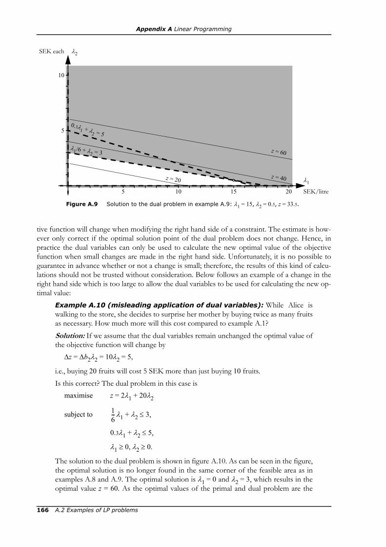
Appendix A Linear Programming
tive function will change when modifying the right hand side of a constraint. The estimate is how-ever only correct if the optimal solution point of the dual problem does not change. Hence, inpractice the dual variables can only be used to calculate the new optimal value of the objectivefunction when small changes are made in the right hand side. Unfortunately, it is no possible toguarantee in advance whether or not a change is small; therefore, the results of this kind of calcu-lations should not be trusted without consideration. Below follows an example of a change in theright hand side which is too large to allow the dual variables to be used for calculating the new op-timal value:
Example A.10 (misleading application of dual variables): While Alice iswalking to the store, she decides to surprise her mother by buying twice as many fruitsas necessary. How much more will this cost compared to example A.1?Solution: If we assume that the dual variables remain unchanged the optimal value ofthe objective function will change by
Δz = Δb2λ2 = 10λ2 = 5,
i.e., buying 20 fruits will cost 5 SEK more than just buying 10 fruits.Is this correct? The dual problem in this case is
maximise z = 2λ1 + 20λ2
subject to λ1 + λ2 ≤ 3,
0.3λ1 + λ2 ≤ 5,
λ1 ≥ 0, λ2 ≥ 0.
The solution to the dual problem is shown in figure A.10. As can be seen in the figure,the optimal solution is no longer found in the same corner of the feasible area as inexamples A.8 and A.9. The optimal solution is λ1 = 0 and λ2 = 3, which results in theoptimal value z = 60. As the optimal values of the primal and dual problem are the
Figure A.9 Solution to the dual problem in example A.9: λ1 = 15, λ2 = 0.5, z = 33.5.
5
5
SEK each λ2
10
10
15 20
λ1/6 + λ2 = 3
0.3λ1 + λ2 = 5
z = 20 z = 40
z = 60
SEK/litre
λ1
16---
166 A.2 Examples of LP problems

Appendix A Linear Programming
same, we can conclude that it will cost Alice 60 SEK to buy at least twenty fruits, i.e.,the real cost increase is 25 SEK.
In an ordinary LP problem the variables may have any value within the variable limits. However,it is also possible to introduce further restrictions to the allowed values of the optimisation varia-bles, namely that some variables may only assume integer values. These problems are called MILPproblems.1
Example A.11 (integer solution): Most shops does not allow the customers to
1. Short for “Mixed Integer Linear Programming”.
Figure A.10 Solution to the dual problem in example A.10: λ1 = 0, λ2 = 3, z = 60.
5
5
SEK each λ2
10
10
15 20
λ1/6 + λ2 = 3
0.3λ1 + λ2 = 5
SEK/litre
λ1z = 20 z = 40
z = 60
Figure A.11 Solution to example A.11: x1 = 7, x2 = 3, z = 36.
5 pears
x1
5
apples x2
10 15
10
z = 70
x1 + x
2 = 10
x1 /6 + 0.3x2 = 2
z = 60
z = 50z = 40
A.2 Examples of LP problems 167
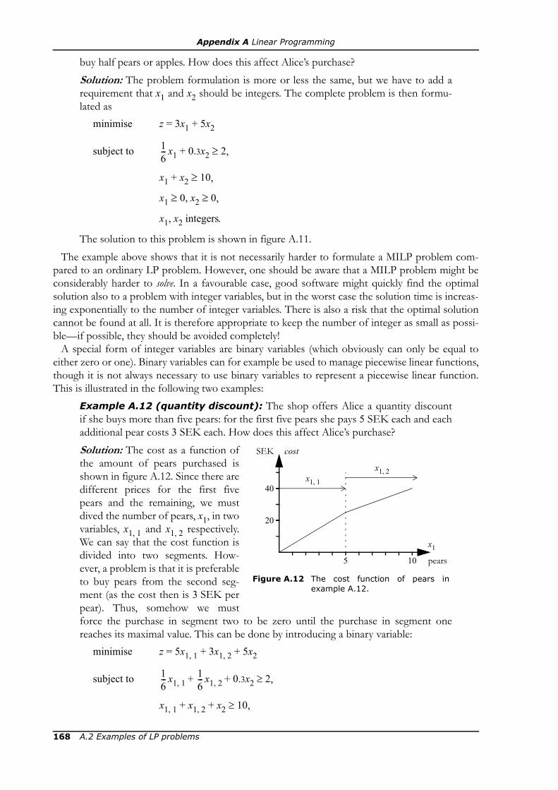
Appendix A Linear Programming
buy half pears or apples. How does this affect Alice’s purchase?Solution: The problem formulation is more or less the same, but we have to add arequirement that x1 and x2 should be integers. The complete problem is then formu-lated as
minimise z = 3x1 + 5x2
subject to x1 + 0.3x2 ≥ 2,
x1 + x2 ≥ 10,
x1 ≥ 0, x2 ≥ 0,
x1, x2 integers.
The solution to this problem is shown in figure A.11.The example above shows that it is not necessarily harder to formulate a MILP problem com-
pared to an ordinary LP problem. However, one should be aware that a MILP problem might beconsiderably harder to solve. In a favourable case, good software might quickly find the optimalsolution also to a problem with integer variables, but in the worst case the solution time is increas-ing exponentially to the number of integer variables. There is also a risk that the optimal solutioncannot be found at all. It is therefore appropriate to keep the number of integer as small as possi-ble—if possible, they should be avoided completely!
A special form of integer variables are binary variables (which obviously can only be equal toeither zero or one). Binary variables can for example be used to manage piecewise linear functions,though it is not always necessary to use binary variables to represent a piecewise linear function.This is illustrated in the following two examples:
Example A.12 (quantity discount): The shop offers Alice a quantity discountif she buys more than five pears: for the first five pears she pays 5 SEK each and eachadditional pear costs 3 SEK each. How does this affect Alice’s purchase?Solution: The cost as a function ofthe amount of pears purchased isshown in figure A.12. Since there aredifferent prices for the first fivepears and the remaining, we mustdived the number of pears, x1, in twovariables, x1, 1 and x1, 2 respectively.We can say that the cost function isdivided into two segments. How-ever, a problem is that it is preferableto buy pears from the second seg-ment (as the cost then is 3 SEK perpear). Thus, somehow we mustforce the purchase in segment two to be zero until the purchase in segment onereaches its maximal value. This can be done by introducing a binary variable:
minimise z = 5x1, 1 + 3x1, 2 + 5x2
subject to x1, 1 + x1, 2 + 0.3x2 ≥ 2,
x1, 1 + x1, 2 + x2 ≥ 10,
16---
5 pears
x1
40
SEK cost
10
20
x1, 1
x1, 2
Figure A.12 The cost function of pears inexample A.12.
16--- 1
6---
168 A.2 Examples of LP problems

Appendix A Linear Programming
x1, 1 – 5s ≥ 0,
– x1, 2 + M·s ≥ 0,
x1, 1 ≥ 0, x1, 2 ≥ 0, x2 ≥ 0, s ∈ {0, 1}.
The objective function now uses the piecewise linear cost function of pears. The firsttwo constraints are more or less the same as in example A.1—the difference is that x1is substituted by x1, 1 + x1, 2. The two new constraints are used to guarantee that x1, 2 iszero unless x1, 1 is equal to five. If the binary variable s is equal to zero then the fourthconstraint (where M denotes an arbitrary large number) forces x1, 2 to be less than orequal to zero. Combined with the variable limit x1, 2 ≥ 0 the only possible solution isx1, 2 = 0. On the other hand, if s is equal to one, the fourth constraint states that x1, 2should be less than or equal to the arbitrary large number M, which in practice is nolimitation. In this case it is the third constraint that is binding, as it forces x1, 1 to be atleast equal to five.Example A.13 (limited offer): Assume that the shop has a special offer insteadof a quantity discount. The special offer is that each customer may buy at most fivepears for 3 SEK each and that each additional pear costs the full price, which is5 SEK each. How does this affect Alice’s purchase?Solution: Alice’s cost function inthis case is shown in figure A.13. Wehave to divide x1 in two segments inthis case too, but the difference isthat now it is purchase in the firstsegment that is most profitable. Inthis case it does not matter if a solu-tion is feasible even though x1, 1 < 5while x1, 2 > 0, because such a solu-tion will not be optimal. Hence, it isunnecessary (but not incorrect) tointroduce a binary variable; every-thing that is needed is a limitationthat x1, 1 may not exceed five. The most simple way of formulating Alice’s problem isthen as follows:
minimise z = 3x1, 1 + 5x1, 2 + 5x2
subject to x1, 1 + x1, 2 + 0.3x2 ≥ 2,
x1, 1 + x1, 2 + x2 ≥ 10,
5 ≥ x1, 1 ≥ 0, x1, 2 ≥ 0, x2 ≥ 0.
FURTHER READING• M. S. Bazaraa, H. D. Sherali & C.M. Shetty, Nonlinear Programming: Theory and Algorithms, second edi-
tion, John Wiley & Sons, 1993. — Complete review of non-linear optimisation. Definitions of many im-portant concepts in optimisation theory.
• S. P. Bradley, A. C. Hax & T. L. Magnanti, Applied Mathematical Programming, Addison-Wesley Publish-ing Company, 1977. — Basic textbook with good examples.
5 pears
x1
40
SEK cost
10
20
x1, 1
x1, 2
Figure A.13 The cost function of pears inexample A.13.
16--- 1
6---
Further Reading 169

Appendix A Linear Programming
• F. S. Hillier & G. J. Lieberman, Introductions to Operations Research, sixth edition, McGraw-Hill, 1995.— Textbook in operations research with good examples.
• S. G. Nash & A. Sofer, Linear and Nonlinear Programming, McGraw-Hill, 1996. — Complete, moderntextbook.
170 Further Reading

Appendix B
SOLVING SHORT-TERMPLANNING PROBLEMS
In this compendium we focus on formulating short-term planning problems, but in practise it isof course also necessary to actually solve them. In a real short-term planning problem there will behundreds or thousands of optimisation variables and then it is of course impossible to solve beproblem by hand calculations. The solution is to use computers and today there is a variety of soft-ware to solve both linear programming problems and other kinds of optimisation problems.
The challenge when using computer software to solve optimisation problems is to ascertain thatthe intended problem has been solved—a small programming error may easily result in an incor-rect solution or an infeasible problem. It is therefore important to be careful both when formulat-ing the optimisation problem and then entering it into the computer. In this appendix we will pro-vide an example of how to set about.
In example 5.6 we formulated a short-term planning problem for two hydro power plants.Below we will show how this problem can be solved using different programming languages.However, let us start with a compilation of the original problem formulation:
Indices of power plants
Degerforsen 1, Edensforsen 2.
Parameters
The following parameters are given:
= installed capacity in power plant i =
= maximal discharge in power plant i =
= maximal contents of reservoir i =
λf = expected future electricity price = 185,
wi = mean annual flow =
Hi62 i 1,=63 i 2,=⎩
⎨⎧
Qi300 i 1,=270 i 2,=⎩
⎨⎧
Mi5 000 000 3 600⁄4 000 000 3 600⁄⎩
⎨⎧ i 1,=
i 2,=
163 i 1,=164 i 2,=⎩
⎨⎧
171

Appendix B Solving Short-term Planning Problems
Dt = contracted load for hour t =
The following parameters are calculated based on the given parameters:Mi, 0 = start contents of reservoir i = i = 1, 2,
Vi = local inflow to reservoir i =
= maximal discharge in power plant i, segment 1 = 0.75 i = 1, 2,
= maximal discharge in power plant i, segment 2 = i = 1, 2,μi, 1 = marginal production equivalent of power plant i, segment 1 =
= i = 1, 2,
μi, 2 = marginal production equivalent of power plant i, segment 2 = 0.95μi, 1.
Optimisation variablesQi, j, t = discharge in power plant i, segment j, during hour t,
i = 1, 2, j = 1, 2, t = 1, …, 6,Si, t = spillage from reservoir i during hour t, i = 1, 2, t = 1, …, 6,
Mi, t = contents of reservoir i at the end of hour t, i = 1, 2, t = 1, …, 6.
Objective function
maximise λf((μ1, 1 + μ2, 1)M1, 6 + μ2, 1M2, 6).
Constraints
M1, t – M1, t – 1 + Q1, 1, t + Q1, 2, t + S1, t = V1, t = 1, … 6,
M2, t – M2, t – 1 + Q2, 1, t + Q2, 2, t + S2, t – Q1, 1, t – Q1, 2, t – S1, t = V2, t = 1, … 6,
= Dt, t = 1, … 6.
Variable limits
0 ≤ Qi, j, t ≤ i = 1, 2, j = 1, 2, t = 1, …, 6,
0 ≤ Si, t, i = 1, 2, t = 1, …, 6,
0 ≤ Mi, t ≤ i = 1, 2, t = 1, …, 6.
9098
104112100
80⎩⎪⎪⎪⎨⎪⎪⎪⎧ t 1,=
t 2,=t 3,=t 4,=t 5,=t 6.=
0.5Mi,w1
w2 w1–⎩⎨⎧ i 1,=
i 2,=
Qi 1, Qi,
Qi 2, Qi Qi 1, ,–
Hi
Qi 1, 0.95Qi 2,+------------------------------------- ,
μi j, Qi j t, ,j 1=
2
∑i 1=
2
∑
Qi j, ,
Mi,
172

Appendix B Solving Short-term Planning Problems
B.1 GAMSGAMS is a programming language especially dedicated to formulation of optimisation problems.The idea is that problems and inputs are formulated in a standardised way—regardless of whetherthe problem at hand is linear or non-linear—and then the problem is passed on to special solvers.A GAMS program is written in an ordinary text file (it is most straightforward to use the built-ineditor). When executing the program (choose Run in the menu File) GAMS will process the fileand check that the problem syntax is correct. If that is the case then the problem is passed to asuitable solver. The solution (or an error message if no solution was found) is then returned toGAMS, where it is possible to choose how to present the results. Finally, the result is written to atext file having the same name as the program file, but with the suffix .lst. This listing file can beviewed in the built-in editor. Any errors encountered during the run results in error messages inthe listing file.
We start by defining the indices to be used in the program. GAMS requires that all possibleindex values are states, in order to allow the program to check that other statements only useallowed values. The syntax for defining index values is
set symbol ”explanatory text” /element1, element2/;
The keyword set (we may also use the plural form sets) states that an index is going to be de-fined, and is followed by the symbol used to denote the index. Then an explanatory text follows,which GAMS will echo when listing the results. The explanatory text may not exceed 80 charac-ters. If no slashes, commas or semi-colons are used in the text, there is no need for the quotationmarks. Finally, the possible index values are listed within the slashes. It is allowed to define morethan one index in the same set statement; the most straightforward is then to define each indexin a row of its own.
Indices of power plants
Degerforsen 1, Edensforsen 2. Setsi power plant/Degerforsen, Edensforsen/
j segment /segment1*segment2/t hour /hour1*hour6/
;
Notice that we may define a sequence of numbered index values using *; the allowed values of theindex t are thus "hour1", "hour2", "hour3", "hour4", "hour5" and "hour6".
The next step is to declare the parameters of the problem. The syntax for declaring parameters issimilar to the one for index values:
Parameters
The following parameters are given:
= installed capacity in power plant i =
=
= maximal discharge in power plant i =
=
ParametersHmax(i) installed capacity in
power plant i/Degerforsen 62,Edensforsen 63/
Qtotmax(i)maximal discharge inpower plant i /Degerforsen 300,Edensforsen 270/
Hi
62 i 1,=63 i 2,=⎩
⎨⎧
Qi
300 i 1,=270 i 2,=⎩
⎨⎧
B.1 GAMS 173

Appendix B Solving Short-term Planning Problems
= maximal contents of reservoir i =
=
λf = expected future electricity price = = 185,
wi = mean annual flow =
=
Dt = contracted load for hour t =
=
Mmax(i) maximal contents of reservoir i/Degerforsen 5e6,Edensforsen 4e6/
lambdaf expected future electricity price /185/
w(i) mean annual flow atpower plant i/Degerforsen 163,Edensforsen 164/
D(t) contracted load hour t /hour1 90, hour2 98,hour3 104, hour4 112,hour5 100, hour6 80/
Mstart(i) start contents of reservoir i
V(i) local inflow to reservoir i
Qmax(i,j) "maximal discharge in power plant i, segment j"
mu(i,j) "marginal productionequivalent for power plant i, segment j"
;
When a parameter has more than one index, a dot is used to separate different index values. Themaximal discharge in each power plant and segment could thus be stated in the following man-ner:1
ParametersQmax(i,j) ”maximal discharge in power plant i, segment j”
/Degerforsen.segment1 225,Edensforsen.segment1 202.5,Degerforsen.segment2 75,Edensforsen.segment2 67.5/
;
However, in order to avoid rounding errors it might be better to let GAMS perform the calcula-tions. In that case, it is sufficient to declare that the parameter exists and then assign values later:The following parameters are calculated based on the given parameters:
Mi, 0 = start contents of reservoir i = i = 1, 2,
Vi = local inflow to reservoir i =
=
Mmax(i) = Mmax(i)/3600;Mstart(i) = 0.5*Mmax(i);V(i) = w(i) - w(i-1);Qmax(i,"segment1") =
0.75*Qtotmax(i);Qmax(i,"segment2") = Qtotmax(i) -
Qmax(i,"segment1");mu(i,"segment1") =
Hmax(i)/(Qmax(i,"segment1") + 0.95*Qmax(i,"segment2"));
mu(i,"segment2") = 0.95*mu(i,"segment1");
Mi
5 000 000 3 600⁄4 000 000 3 600⁄⎩
⎨⎧ i 1,=
i 2,=
163 i 1,=164 i 2,=⎩
⎨⎧
9098
10411210080⎩
⎪⎪⎪⎨⎪⎪⎪⎧ t 1,=
t 2,=t 3,=t 4,=t 5,=t 6.=
1. An alternative approach would be to use the key word Table. See GAMS Users Guide (which can beaccessed from the help menu in the GAMS window) for further details.
0.5Mi,
w1
w2 w1–⎩⎨⎧ i 1,=
i 2,=
174 B.1 GAMS

Appendix B Solving Short-term Planning Problems
= maximal discharge in power plant i,
segment 1 = 0.75 i = 1, 2,
= maximal discharge in power plant i,
segment 2 = i = 1, 2,
μi, 1 = marginal production equivalent ofpower plant i, segment 1 =
= i = 1, 2,
μi, 2 = marginal production equivalent ofpower plant i, segment 2 = 0.95μi, 1.
Notice that GAMS automatically performs assignments over all possible values of the indicesinvolved in the expression. Thus, the first row in the code above will be interpreted by GAMS as
Mmax(”Degerforsen”) = Mmax(”Degerforsen”)/3600;
andMmax(”Edensforsen”) = Mmax(”Edensforsen”)/3600;
Another feature of GAMS is that expressions which contain non-existing index values will auto-matically be removed from the calculations. When the index i is equal to "Edensforsen" therow
V(i) = w(i) - w(i-1);
is read as V("Edensforsen") = w("Edensforsen") - w("Degerforsen");
i.e., i – 1 is automatically replaced by the previous index value. But when i is equal to"Degerforsen" there is no previous index value (as "Degerforsen" is the first powerplant in the definition of the set); hence this part is removed and then the row reads
V("Degerforsen") = w("Degerforsen");
We must also declare which optimisation variables we have in the problem. Notice that wealready now can state some variable limits by using the keywords positive, negative,binary, integer and free. GAMS requires that there is at least one free variable in eachproblem, as the variable to be maximised or minimised must be able to assume any value. The dec-larations are similar to the index values and parameters, i.e., a symbol is stated followed by anexplanatory text (however, no values are stated):
Optimisation variables
Qi, j, t = discharge in power plant i, segment j, during hour t, i = 1, 2,j = 1, 2, t = 1, …, 6,
Si, t = spillage from reservoir i during hour t, i = 1, 2, t = 1, …, 6,
Mi, t = contents of reservoir i at the end of hour t, i = 1, 2, t = 1, …, 6.
Positive variablesQ(i,j,t) "discharge in power
plant i, segment j, during hour t"
S(i,t) spillage from reservoir i during hour t
M(i,t) contents of reservoir i at the end of hour t
Qi 1,
Qi,
Qi 2,
Qi Qi 1, ,–
Hi
Qi 1, 0.95Qi 2,+------------------------------------- ,
B.1 GAMS 175

Appendix B Solving Short-term Planning Problems
;
Free variablez value of stored water
;
The relation between the optimisation variables are described by equations in GAMS. An equa-tion must first be declared; this is done in a similar manner as for variables. Then, the actual equa-tion is defined according to the following syntax:
symbol .. LHS type RHS;
Here, symbol is the name the equation was given when declared. The name of the equation isseparated from the equation definition by two dots. Both the left hand side (LHS) and right handside (RHS) are mathematical expressions. The relation between the left and right hand sides aredepending on the type of the equation (see table B.1). There is no difference in syntax betweenthe objective function and the constraints; the objective function is simply the equation stating thevalue of the free variable to be minimised or maximised:
Objective function
maximise λf((μ1, 1 + μ2, 1)M1, 6 + μ2, 1M2, 6). Equationobjfnc objective function;
objfnc.. z =e= lambdaf*((mu("Degerforsen",
"segment1") +mu("Edensforsen", "segment1"))
*M("Degerforsen","hour6")
+ mu("Edensforsen","segment1")
*M("Edensforsen","hour6"));
The constraints are also stated as equations. Once again we can utilise that GAMS removesexpressions if the index value does not exist. However, in the hydrological constraints there is acomplication, which cannot be managed by GAMS itself. In the first hour there is no optimisationvariable Mi, t – 1, but there is a parameter Mi, 0, which in the program has been given the symbolMstart(i). This parameter should only be included in those hydrological constraints for whicht is equal to "hour1". This is implemented by using a so-called dollar condition, which meansthat after an expression we may type a $-sign, followed by a condition. If this condition is not ful-filled the expression will be removed, in the same way as non-existing index values are removed.The function ord can be used to obtain the position of an index value in a set. As "hour1" isthe first value in the set t, the condition ord(t) = 1 will only be fulfilled for the hydrologicalbalances during the first hour.
Table B.1 GAMS equation types.
Type of equations
Mathematical symbol Sense
=e= = Left hand side must equal right hand side=l= ≤ Left hand side must be less than or equal to the right hand side=g= ≥ Left hand side must be greater than or equal to right hand side
176 B.1 GAMS
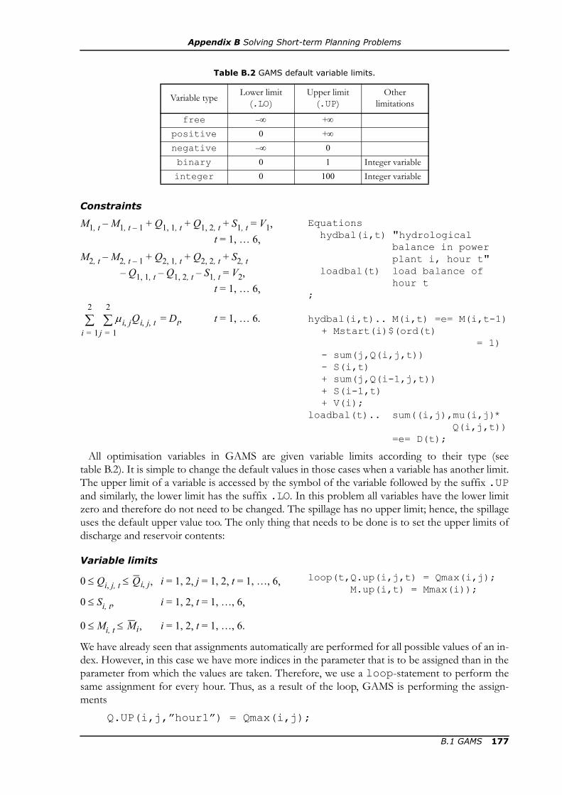
Appendix B Solving Short-term Planning Problems
Constraints
M1, t – M1, t – 1 + Q1, 1, t + Q1, 2, t + S1, t = V1,t = 1, … 6,
M2, t – M2, t – 1 + Q2, 1, t + Q2, 2, t + S2, t – Q1, 1, t – Q1, 2, t – S1, t = V2,
t = 1, … 6,
= Dt, t = 1, … 6.
Equationshydbal(i,t) "hydrological
balance in power plant i, hour t"
loadbal(t) load balance of hour t
;
hydbal(i,t).. M(i,t) =e= M(i,t-1)+ Mstart(i)$(ord(t)
= 1)- sum(j,Q(i,j,t))- S(i,t)+ sum(j,Q(i-1,j,t))+ S(i-1,t)+ V(i);
loadbal(t).. sum((i,j),mu(i,j)*Q(i,j,t))
=e= D(t);
All optimisation variables in GAMS are given variable limits according to their type (seetable B.2). It is simple to change the default values in those cases when a variable has another limit.The upper limit of a variable is accessed by the symbol of the variable followed by the suffix .UPand similarly, the lower limit has the suffix .LO. In this problem all variables have the lower limitzero and therefore do not need to be changed. The spillage has no upper limit; hence, the spillageuses the default upper value too. The only thing that needs to be done is to set the upper limits ofdischarge and reservoir contents:
Variable limits
0 ≤ Qi, j, t ≤ i = 1, 2, j = 1, 2, t = 1, …, 6,
0 ≤ Si, t, i = 1, 2, t = 1, …, 6,
0 ≤ Mi, t ≤ i = 1, 2, t = 1, …, 6.
loop(t,Q.up(i,j,t) = Qmax(i,j);M.up(i,t) = Mmax(i));
We have already seen that assignments automatically are performed for all possible values of an in-dex. However, in this case we have more indices in the parameter that is to be assigned than in theparameter from which the values are taken. Therefore, we use a loop-statement to perform thesame assignment for every hour. Thus, as a result of the loop, GAMS is performing the assign-ments
Q.UP(i,j,”hour1”) = Qmax(i,j);
μi j, Qi j t, ,j 1=
2
∑i 1=
2
∑
Table B.2 GAMS default variable limits.
Variable type Lower limit (.LO)
Upper limit (.UP)
Other limitations
free –∞ +∞
positive 0 +∞
negative –∞ 0binary 0 1 Integer variableinteger 0 100 Integer variable
Qi j, ,
Mi,
B.1 GAMS 177

Appendix B Solving Short-term Planning Problems
M.UP(i,”hour1”) = Mmax(i);
Q.UP(i,j,”hour2”) = Qmax(i,j);
M.UP(i,”hour2”) = Mmax(i);
etc.We can now solve the problem. First we give a name to the model, while stating which equations
are included in the model (in this case it is all equations, which is stated by /all/). Then we askGAMS to solve the optimisation problem. First, we must specify which type of solver that is to beused. In this case we have an LP problem; therefore, we state that the problem should be solved“using lp”. It we would like to solve a MILP problem, we would have stated “using mip”,and if we would like to solve a non-linear problem, we would state “using nlp”. GAMS willautomatically select the solver which is most appropriate for problems of the specified type.Finally, we must state which variable is to be minimised or maximised. In this case it is z that shallbe maximised. Remember that the variable to be maximised or minimised must be declared as afree variable.
model hydroplanning /all/;
solve hydroplanning using lp maximizing z;
Finally we instruct GAMS to write the most important results at the end of the listing file. At thesame time, we can also calculate the total discharge and electricity generation in each power plantand hour (cf. the discharge plan in table 5.5). To calculate the total discharge and electricity gener-ation we need the optimal values of the discharge Vi, j, t. When GAMS is solving the optimisationproblem the optimal solution is stored in parameters having the same name as the optimisationvariable followed by the suffix .L. Hence, the optimal discharge is accessed through Q.L. We canalso obtain the dual variables of both constraints and variable limits. The dual variables are storedin parameters which have the same name as the constraint or the optimisation variable followed bythe suffix .M.
ParametersQtot(i,t) "total discharge in
power plant i, hour t"
H(i,t) "generation in power plant i, hour t"
;
loop((i,t),Qtot(i,t) =sum(j,Q.L(i,j,t));H(i,t) = sum(j,mu(i,j)*Q.L(i,j,t)));
display M.L, Q.L, Qtot, H, S.L;display hydbal.M, loadbal.M;
B.2 MATLABMatlab is a general programming language for technical computing. There is a large range ofready-made functions for many areas of computing. With the exception of the most basic mathe-matical functions—which are included in the software—all functions are written in ordinary textfiles (it is most straightforward to use the built-in editor).
178 B.2 Matlab

Appendix B Solving Short-term Planning Problems
Functions to solve optimisation problems are found in the so-called Matlab OptimizationToolbox, but there are also freeware functions to be found on the Internet. Below it is demon-strated how our problem can be solved using linprog (which is included in OptimizationToolbox). As most Matlab functions for solving LP problems, linprog requires that the prob-lem is formulated using matrices. In this case the problem should be on the form
minimise fTx (B.1)
subject to Ax ≤ b, (B.1a)
Aeqx = beq, (B.1b)
lb ≤ x ≤ ub. (B.1c)
The function linprog can be called with different inputs and outputs, depending on how wewish to use the function.2 Below follows a description of what is needed to solve the example inthis appendix.
Assume that a problem has Nineq inequality constraints, Neq equality constraints and M variables.In that case linprog uses the following inputs:
f coefficients of the objective function (column vector with M elements),A coefficients of the inequality constraints (matrix with Nineq rows and M col-
umns),b right hand side of the inequality constraints (column vector with Nineq ele-
ments),Aeq coefficients of the equality constraints (matrix with Neq rows and M col-
umns),beq right hand side of the equality constraints (column vector with Neq ele-
ments),lb lower bound of the optimisation variables (column vector with M elements),ub upper bound of the optimisation variables (column vector with M elements).
The result of a call is x optimal solution (column vector with M elements).
The difficulty when solving the planning problem is to correctly define the inputs necessary tocall linprog. To make sure that no mistakes are made in this process, it is appropriate to write aMatlab program which follows the original problem formulation as closely as possible. Hence, westart by clarifying the index values we use for the power plants:
Indices of power plants
Degerforsen 1, Edensforsen 2. % Indices of the power plants:% Degerforsen 1, Edensforsen 2
In Matlab everything on a row after a %-sign is considered a comment. Hence, no calculations areperformed by the two rows above—they are just intended to make the program easier to under-stand.
The next step is to define all parameter values:
2. Please refer to the built-in help function of Matlab for a more detailed description.
B.2 Matlab 179

Appendix B Solving Short-term Planning Problems
Parameters
The following parameters are given:
= installed capacity in power plant i =
=
= maximal discharge in power plant i =
=
= maximal contents of reservoir i =
=
λf = expected future electricity price = = 185,
wi = mean annual flow =
=
Dt = contracted load for hour t =
=
Given parametersnpowerplants = 2;nhours = 6;Hmax = [62; 63]; % Hmax(i)Qtotmax = [300; 270];
% Qtotmax(i)Mmax = [5e6; 4e6]/3600; % Mmax(i)lambdaf = 185;w = [163; 164]; % w(i)D = [90 98 104 112 100 80];
% D(t)
The following parameters are calculated based on the given parameters:
Mi, 0 = start contents of reservoir i = i = 1, 2,
Vi = local inflow to reservoir i =
=
= maximal discharge in power plant i,
segment 1 = 0.75 i = 1, 2,
% Calculated parametersMstart = 0.5*Mmax; % Mstart(i)V = [w(1); w(2)-w(1)]; % V(i)% Qmax(i,j)Qmax(:,2) = Qtotmax - Qmax(:,1);Qmax(:,1) = .75*Qtotmax;% mu(i,j)mu(:,1) = Hmax./(Qmax(:,1) +
0.95*Qmax(:,2));mu(:,2) = 0.95*mu(:,1);
Hi
62 i 1,=63 i 2,=⎩
⎨⎧
Qi
300 i 1,=270 i 2,=⎩
⎨⎧
Mi
5 000 000 3 600⁄4 000 000 3 600⁄⎩
⎨⎧ i 1,=
i 2,=
163 i 1,=164 i 2,=⎩
⎨⎧
9098
10411210080⎩
⎪⎪⎪⎨⎪⎪⎪⎧ t 1,=
t 2,=t 3,=t 4,=t 5,=t 6.=
0.5Mi,
w1
w2 w1–⎩⎨⎧ i 1,=
i 2,=
Qi 1,
Qi,
180 B.2 Matlab
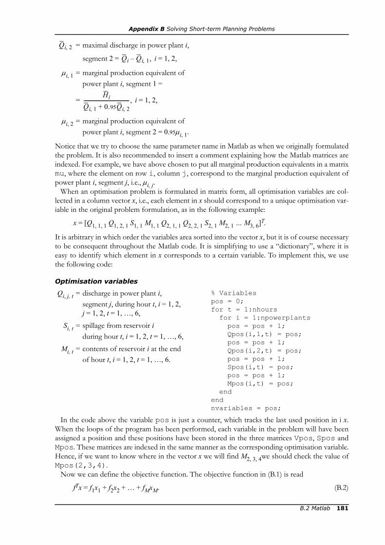
Appendix B Solving Short-term Planning Problems
= maximal discharge in power plant i,
segment 2 = i = 1, 2,
μi, 1 = marginal production equivalent ofpower plant i, segment 1 =
= i = 1, 2,
μi, 2 = marginal production equivalent ofpower plant i, segment 2 = 0.95μi, 1.
Notice that we try to choose the same parameter name in Matlab as when we originally formulatedthe problem. It is also recommended to insert a comment explaining how the Matlab matrices areindexed. For example, we have above chosen to put all marginal production equivalents in a matrixmu, where the element on row i, column j, correspond to the marginal production equivalent ofpower plant i, segment j, i.e., μi, j.
When an optimisation problem is formulated in matrix form, all optimisation variables are col-lected in a column vector x, i.e., each element in x should correspond to a unique optimisation var-iable in the original problem formulation, as in the following example:
x = [Q1, 1, 1 Q1, 2, 1 S1, 1 M1, 1 Q2, 1, 1 Q2, 2, 1 S2, 1 M2, 1 … M3, 6]T.
It is arbitrary in which order the variables area sorted into the vector x, but it is of course necessaryto be consequent throughout the Matlab code. It is simplifying to use a “dictionary”, where it iseasy to identify which element in x corresponds to a certain variable. To implement this, we usethe following code:
Optimisation variables
Qi, j, t = discharge in power plant i, segment j, during hour t, i = 1, 2,j = 1, 2, t = 1, …, 6,
Si, t = spillage from reservoir i during hour t, i = 1, 2, t = 1, …, 6,
Mi, t = contents of reservoir i at the end of hour t, i = 1, 2, t = 1, …, 6.
% Variablespos = 0;for t = 1:nhoursfor i = 1:npowerplantspos = pos + 1; Qpos(i,1,t) = pos;pos = pos + 1; Qpos(i,2,t) = pos;pos = pos + 1; Spos(i,t) = pos;pos = pos + 1; Mpos(i,t) = pos;
endendnvariables = pos;
In the code above the variable pos is just a counter, which tracks the last used position in i x.When the loops of the program has been performed, each variable in the problem will have beenassigned a position and these positions have been stored in the three matrices Vpos, Spos andMpos. These matrices are indexed in the same manner as the corresponding optimisation variable.Hence, if we want to know where in the vector x we will find M2, 3, 4we should check the value ofMpos(2,3,4).
Now we can define the objective function. The objective function in (B.1) is read
fTx = f1x1 + f2x2 + … + fMxM. (B.2)
Qi 2,
Qi Qi 1, ,–
Hi
Qi 1, 0.95Qi 2,+------------------------------------- ,
B.2 Matlab 181

Appendix B Solving Short-term Planning Problems
When calling linprog we just need to state the coefficients, f. If we look at the problem formu-lation we find that only two optimisation variables are included in the objective function, whichmeans that most of the coefficients in f are equal to zero. To shorten the Matlab code we can startby a vector of the right size, which just hold zeros (such a vector is generated by the functionzeros). Then we change just those coefficients that are non-zero. For example, the coefficientbefore M2, 6 is equal to μ2, 1 and if M2, 6 is the n:th element of the vector x then the n:th element off should equal μ2, 1. To know the position of M2, 6 we use the earlier defined “dictionary” Mpos:
Objective function
maximise λf((μ1, 1 + μ2, 1)M1, 6 + μ2, 1M2, 6). % Objective function:f = zeros(nvariables,1);f(Mpos(1,nhours)) = ...
lambdaf*(mu(1,1) + mu(2,1));f(Mpos(2,nhours)) = ...
lambdaf*mu(2,1);
The constraints are built in a similar manner as the objective function. Each constraint corre-sponds to a certain row in the matrices A and Aeq respectively, and a certain row in the columnvectors b and beq respectively. We use a counter cnstr to keep track of which constraint we cur-rently define; each time we start stating the coefficients of a new constraint we first increase thevalue of cnstr by one.
Notice that in the hydrological constraints we are forced to use an if-clause to manage differentcases. The first hour (i.e., then t = 1) the reservoir contents at the end of the previous hour is aknown parameter, which should be added to the right hand side of the constraint, whereas Mi, t – 1is an optimisation variable for the other hours. Moreover, in the hydrological balance of Degerfor-sen (which we defined as power plant 1) there is no incoming water from discharge and spillage inthe power plant upstream; hence, these coefficients should only be included if i > 1.
Constraints
M1, t – M1, t – 1 + Q1, 1, t + Q1, 2, t + S1, t = V1,t = 1, … 6,
M2, t – M2, t – 1 + Q2, 1, t + Q2, 2, t + S2, t – Q1, 1, t – Q1, 2, t – S1, t = V2,
t = 1, … 6,
= Dt, t = 1, … 6.
% Constraintsnconstraints = 3*nhours;Aeq = zeros(nconstraints,...
nvariables);beq = zeros(nconstraints,1);cnstr = 0;for t = 1:nhoursfor i = 1:npowerplantscontrnr = cnstr + 1;Aeq(cnstr,Mpos(i,t)) = 1;if k == 1beq(cnstr) = beq(cnstr) ...
+ Mstart(i);elseAeq(cnstr,Mpos(i,t-1)) ... = -1;
endAeq(cnstr,Qpos(i,1,t)) = 1;Aeq(cnstr,Qpos(i,2,t)) = 1;Aeq(cnstr,Spos(i,t)) = 1;if i > 1Aeq(cnstr,Qpos(i-1,1,t))... = -1;
μi j, Qi j t, ,j 1=
2
∑i 1=
2
∑
182 B.2 Matlab

Appendix B Solving Short-term Planning Problems
Aeq(cnstr,Qpos(i-1,2,t))...= -1;
Aeq(cnstr,Spos(i-1,t))...= -1;
endbeq(cnstr) = beq(cnstr) + ...
V(i);endcnstr = cnstr + 1;for i = 1:npowerplantsfor j = 1:2Aeq(cnstr,Qpos(i,j,t)) = ...mu(i,j);
endendbeq(cnstr) = D(t);
end
Finally we have to define the upper and lower limits on all optimisation variables. The lower lim-its are all zeros; therefore, the vector lb is easily defined directly by the function zeros. Theupper limits are different for different variables. The most common limit is +∞ and we may there-fore start from a vector of the correct size, where all elements are equal to +∞ (such a vector canbe generated by the function inf) and then we change the upper limits that are not infinite:
Variable limits
0 ≤ Qi, j, t ≤ i = 1, 2, j = 1, 2, t = 1, …, 6,
0 ≤ Si, t, i = 1, 2, t = 1, …, 6,
0 ≤ Mi, t ≤ i = 1, 2, t = 1, …, 6.
% Variable limits:lb = zeros(nvariables,1);ub = inf(nvariables,1);for t = 1:nhoursfor i = 1:npowerplantsfor j = 1:2ub(Qpos(i,j,t)) = ...
Vmax(i,j);endub(Mpos(i,t)) = Mmax(i);
endend
Now that all inputs have been defined (we have no inequality constraints, so there is no need todefine A and b; they are replaced by empty matrices in the call to linprog) and are ready tosolve the optimisation problem. As linprog solves a minimisation problem and we have formu-lated a maximisation problem we must remember to negate the objective function! The functionlinprog can in addition to the optimal solution also return additional information about theproblem. For example is the value of the dual variables of both constraints and variable limits cal-culated. The dual variables are the fifth value returned by linprog. Hence, we are only inter-ested of the first and fifth value, and the values in between are stored in the waste parameterswaste1, waste2 and waste3:
% Solve the optimisation problem:[x,waste1,waste2,waste3,y] =
linprog(-f,[],[],...Aeq,beq,lb,ub);
The function returns the optimal solution stored in the vector x. To get a better overview of theoptimal solution we can extract the individual optimisation variables and put them in separate
Qi j, ,
Mi,
B.2 Matlab 183

Appendix B Solving Short-term Planning Problems
matrices for each kind of variable (discharge, spillage and reservoir contents). At the same time, wecan also calculate the total discharge and electricity generation in each power plant and hour (cf.the discharge plan in table 5.5). The dual variables are returned in a Matlab structure. A dot fol-lowed by the field name in question is used to access a field in the structure., The structure storingthe dual variables has the fields .ineqlin (dual variables of the inequality constraints),.eqlin (dual variables of the equality constraints), .upper (dual variables of the upper variablelimits) and .lower (dual variables of the lower variable limits).
% Sort the results:Qres = [];Sres = [];Mres = [];for t = 1:nhoursfor i = 1:npowerplantsfor j = 1:2Qres(i,j,t) = ...
x(Vpos(i,j,t));endSres(i,t) = x(Spos(i,t));Mres(i,t) = x(Mpos(i,t));Qtot(i,t) = sum(Qres(i,:,t));H(i,t) = ...mu(i,1)*Qres(i,1,t) + ...mu(i,2)*Qres(i,2,t);
endendoptvalue = round(f’*x)Mres, Qres, Qtot, H, Sresdualvariables = y.eqlin
184 B.2 Matlab
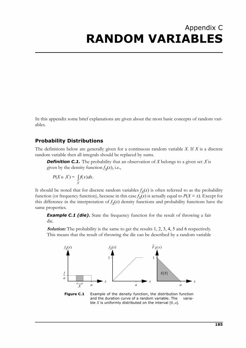
Appendix C
RANDOM VARIABLES
In this appendix some brief explanations are given about the most basic concepts of random vari-ables.
Probability Distributions
The definitions below are generally given for a continuous random variable X. If X is a discreterandom variable then all integrals should be replaced by sums.
Definition C.1. The probability that an observation of X belongs to a given set X isgiven by the density function fX(x), i.e.,
P(X ∈X ) =
It should be noted that for discrete random variables fX(x) is often referred to as the probabilityfunction (or frequency function), because in this case fX(x) is actually equal to P(X = x). Except forthis difference in the interpretation of fX(x) density functions and probability functions have thesame properties.
Example C.1 (die). State the frequency function for the result of throwing a fairdie.Solution: The probability is the same to get the results 1, 2, 3, 4, 5 and 6 respectively.This means that the result of throwing the die can be described by a random variable
f x( ) x.dX∫
a
1a---
fX(x)
xa
fX(x)
xa
xX
11
E[X]
Figure C.1 Example of the density function, the distribution functionand the duration curve of a random variable. The varia-ble X is uniformly distributed on the interval [0, a].
FX x( )
185
Appendix C Random Variables
X, where the probabilities of each of the six possible outcomes are equal, i.e.,
fX(x) =
Definition C.2. The probability that X ≤ x is given by the distribution functionFX(x), i.e., FX(x) = P(X ≤ x).Definition C.3. The probability that X > x is given by the duration curve i.e.,
= P(X > x).Theorem C.4. The density function, the distribution function and the durationcurve are related through
= 1 – FX(x) = =
Proof: The first two equalities follow directly from definitions C.1-C.3. The last equal-ity is obtained by observing that the probability of X ∈ R is exactly 100%, which canbe written as
⇔
Example C.2. What is the probability that the result of throwing a die is not largerthan 3?Solution: The probability that X ≤ 3 is given by
FX(3) = = 0.5.
When adding two random variables the result will be a new random variable having a probabilitydistribution of its own. The following applies to independent variables:1
Theorem C.5. The density function of the sum, Z, of two independent random var-iables X and Y can be obtained by a convolution formula. For independent discreterandom variables the convolution formula is written as
fZ(x) =
and for independent continuous random variables it reads
fZ(x) =
Convolution can also be applied to distribution functions and duration curves.Example C.3. Assume that you have two fair dice and that X is the outcome of onedie and Y is the outcome of the other die. What is the probability that the sum of bothoutcomes is equal to 9?Solution: Both dice have the same frequency function as in example C.1, i.e.,
1. See the section Correlations on page 188.
16---
0⎩⎪⎨⎪⎧
x 1 2 3 4 5 6---, , , , ,=
all other x.
FX x( ),FX x( )
FX x( ) 1 fX t( ) td∞–
x
∫– fX t( ) t.dx
∞
∫
fX t( ) td∞–
∞
∫ 1= fX t( ) td∞–
x
∫ fX t( ) tdx
∞
∫+ 1.=
fX i( )i 1=
3
∑ 36---=
fX i( )fY x i–( )i
∑
fX t( )fY x t–( ) t.d∞–
∞
∫
186

Appendix C Random Variables
fY(x) = fX(x). Let Z = X + Y. The probability that Z = 9 is given by
fZ(9) = = fX(3)·fY(6) + fX(4)·fY(5) + fX(5)·fY(4) + fX(6)·fY(3) =
=
Expectation Value and Variance
The density and distribution functions defined above provide detailed information about a ran-dom variable. In many cases it is of larger practical importance to just know the expected averageand a measure of how much a single sample can diverge from the average. This information isgiven by the expectation value and the variance:
Definition C.6. The expectation value of a random variable X is given by
E[X] =
Definition C.7. The variance of a random variable X is equal to the expected squareof the deviation from the average, i.e.,
Var[X] = E[(X – E[X])2] =
Another common measure is the standard deviation, which simply is the square root of the vari-ance.
Example C.4. Calculate the expectation value, variance and standard deviation of afair die.Solution:
E[X] = = 3.5.
Var[X] = =
= ≈ 2.92.
σX = = ≈ 1.71.
The following two theorems show how the expectation value and variance are affected by linearoperations:
Theorem C.8. If a random variable X is multiplied by a scalar a then the expectationvalue and variance of aX is given by
E[aX] = aE[X],
Var[aX] = Var[X].
Theorem C.9. The expectation value and variance of the sum of two random varia-bles X and Y are given by
fX i( )fY 9 i–( )i 3=
6
∑
16--- 1
6--- 1
6--- 1
6--- 1
6--- 1
6--- 1
6--- 1
6---⋅+⋅+⋅+⋅ 4
36------ .=
xfX x( ) x.d∞–
∞
∫
x E X[ ]–( )2fX x( ) x.d∞–
∞
∫
xfX x( )x 1=
6
∑ 16--- x
x 1=
6
∑ 1 2 3 4 5 6+ + + + +6
------------------------------------------------- 216------= = =
x E X[ ]–( )2fX x( )x 1=
6
∑ x2fX x( ) E X[ ]( )2–x 1=
6
∑ 16--- x2 3,5–
x 1=
6
∑= =
1 4 9 16 25 36+ + + + +6
---------------------------------------------------------- 216
------⎝ ⎠⎛ ⎞ 2
– 3512------=
Var X[ ] 3512------
a2
187
Appendix C Random Variables
E[X + Y] = E[X] + E[Y],Var[X + Y] = Var[X] + Var[Y] + 2Cov[X, Y].
In this compendium we will often use duration curves to describe random variables. One of thereasons why duration curves are useful is that it is possible to calculate the expectation value of thecorresponding random variable by studying the area below the duration curve:
Theorem C.10. If is the smallest possible outcome of X then the expectationvalue of X is given by
E[X] = + .
In power system analysis the smallest possible outcome s often equal to zero, which means thatthe expectation value is equal to the area below the part of the duration curve which belongs tothe first quadrant. This is illustrated in figure C.1.
Correlations
When studying more than one random variable it is generally very important to know how theirprobability distributions are related to each other. A very important notion in this context is inde-pendent random variables. There are several definitions of independent random variables, but sim-ply speaking, two random variables are X and Y are independent if the outcome of X does not af-fect the outcome of Y and vice versa. For example, if a dice is rolled twice, and X is the firstoutcome and Y the second, then X and Y should be independent.2 If X is the first outcome and Yis the sum of the two results, then X and Y are dependent; Y will have different probability func-tions when the outcome of X is known.
One measure of how the probability distributions of two random variables are correlated to eachother is the covariance:
Definition C.11. The covariance of two random variables X and Y is given byCov[X, Y] = E[(X – E[X])(Y – E[Y])].
A related notion is the correlation coefficient:Definition C.12. The correlation coefficient of two random variables X and Y isgiven by
ρX, Y = .
The correlation coefficient will always be in the interval [–1, 1]. If ρ(X, Y) = 0 the variables X and Yare considered to be uncorrelated. Independent variables are always uncorrelated, but the converseis not always true.3 If ρ(X, Y) is positive, then the variables are positively correlated, which meansthat if we for example know that the outcome of X was higher than the average, then it is morelikely that also Y was over the average. If the variables instead are negatively correlated (ρ(X,Y) < 0) then a high value of X result in an increased probability of a low value of Y.
2. Unless there is something fishy about the dice.3. Consider for example a U(–1, 1)-distributed random variable X and Y = X2. Although Y is clearly depend-
ing on X, the correlation coefficient ρ(X, Y) = 0.
x
x FX˜ x( ) xd
x
∞
∫
x
Cov X Y,[ ]Var X[ ]Var Y[ ]
---------------------------------------
188

Appendix D
THE NORMALDISTRIBUTION
The normal distribution (also referred to as theGaussian distribution) is a probability distributionwhich have a lot of uses. A general normal distribu-tion is characterised by two parameters: the mean μand the standard deviation σ.
Definition D.1. A random variable X isnormally distributed if it has the followingdensity and distribution functions:
fX(x) =
and
FX(x) =
This is denoted X ∈ N(μ, σ).Using the definitions of expectation value andstandard deviation it is possible to control that thedensity function and distribution functions abovecorrespond to the expectation value μ and standarddeviation σ.
An important special case is when the mean iszero and the standard deviation is equal to one:
Definition D.2. The standardised normaldistribution has μ = 0 and σ = 1. The densityfunction of an N(0, 1)-distributed randomvariable is denoted ϕ(x) and the distribution function is denoted Φ(x).
Figure D.1 shows ϕ(x) and Φ(x). Notice the symmetry!Theorem D.3. If X ∈ N(μ, σ) then Y = (X – μ)/σ ∈ N(0, 1).
From theorem D.3 we can conclude that if Y ∈ N(0, 1) then X = μ + σY ∈ N(μ, σ). The practicalimportance of the theorem is that the standardised normal distribution can be used for calcula-
–1
x
–2 1 32
0.4
0.2
–3
ϕ(x)
0.3
0.1
–1
x
–2 1 32
1
0.5
–3
Φ(x)
0.75
0.25
Figure D.1 The density function and distri-bution function of the standard-ised normal distribution.
1σ 2π--------------e
x μ–( )2
2σ2-------------------–
1σ 2π-------------- e
y μ–( )2
2σ2-------------------–
y.d∞–
x
∫
189

Appendix D The Normal Distribution
tions of a general normal distribution.Example D.1. The random variable X is normally distributed with μ = 100 andσ = 50. Calculate the probability that X is larger than 90.Solution: According to the definition we have
P(X > 90) = 1 – P(X ≤ 90) = 1 – FX(90) = 1 – = 1 – Φ(–0.2) =
= {symmetry} = 1 – (1 – Φ(0.2)).
The value of Φ(0.2) can be calculated on a computer or found in table D.1; the resultis that the probability of X > 90 is about 57.93%.
An advantage of the normal distribution is that it is easy to add normally distributed variables:Theorem D.4. Assume that there are independent normally distributed random var-iables, X1 ∈ N(μ1, σ1), …,Xn ∈ N(μn, σn). Then it holds that the sum is
Example D.2. Assume that X ∈ N(100, 30) and Y ∈ N(200, 40) and that X and Y areindependent. Calculate the probability that the sum of these variables is larger than350.Solution: If Z = X + Y then Z is, according to theorem D.4, normally distributed withthe mean
μZ = 100 + 200 = 300
and the standard deviation
σZ = = 50.
Hence we get,
P(X + Y > 350) = 1 – = 1 – Φ(1) ≈ 0,1587.
Table
A table of the distribution function of the standardised normal distribution, i.e.,
Φ(x) =
is given below. For x < 0 we can calculate Φ(x) usingΦ(–x) = 1 – Φ(x).
Φ 90 μ–σ
---------------⎝ ⎠⎛ ⎞
ciXii 1=
n
∑ N ciμii 1=
n
∑ ci2σi
2
i 1=
n
∑,⎝ ⎠⎜ ⎟⎛ ⎞
.∈
302 402+
Φ 350 300–50
------------------------⎝ ⎠⎛ ⎞
12π
---------- ey2
2-----–
yd∞–
x
∫
190

Appendix D The Normal Distribution
Table D.1 The distribution function of the standardised normal distribution.
x .00 .01 .02 .03 .04 .05 .06 .07 .08 .09
0.0 0.50000 0.50399 0.50798 0.51197 0.51595 0.51994 0.52392 0.52790 0.53188 0.535860.1 0.53983 0.54380 0.54776 0.55172 0.55567 0.55962 0.56356 0.56749 0.57142 0.575350.2 0.57926 0.58317 0.58706 0.59095 0.59483 0.59871 0.60257 0.60642 0.61026 0.614090.3 0.61791 0.62172 0.62552 0.62930 0.63307 0.63683 0.64058 0.64431 0.64803 0.651730.4 0.65542 0.65910 0.66276 0.66640 0.67003 0.67364 0.67724 0.68082 0.68439 0.68793
0.5 0.69146 0.69497 0.69847 0.70194 0.70540 0.70884 0.71226 0.71566 0.71904 0.722400.6 0.72575 0.72907 0.73237 0.73565 0.73891 0.74215 0.74537 0.74857 0.75175 0.754900.7 0.75804 0.76115 0.76424 0.76730 0.77035 0.77337 0.77637 0.77935 0.78230 0.785240.8 0.78814 0.79103 0.79389 0.79673 0.79955 0.80234 0.80511 0.80785 0.81057 0.813270.9 0.81594 0.81859 0.82121 0.82381 0.82639 0.82894 0.83147 0.83398 0.83646 0.83891
1.0 0.84134 0.84375 0.84614 0.84849 0.85083 0.85314 0.85543 0.85769 0.85993 0.862141.1 0.86433 0.86650 0.86864 0.87076 0.87286 0.87493 0.87698 0.87900 0.88100 0.882981.2 0.88493 0.88686 0.88877 0.89065 0.89251 0.89435 0.89617 0.89796 0.89973 0.901471.3 0.90320 0.90490 0.90658 0.90824 0.90988 0.91149 0.91309 0.91466 0.91621 0.917741.4 0.91924 0.92073 0.92220 0.92364 0.92507 0.92647 0.92785 0.92922 0.93056 0.93189
1.5 0.93319 0.93448 0.93574 0.93699 0.93822 0.93943 0.94062 0.94179 0.94295 0.944081.6 0.94520 0.94630 0.94738 0.94845 0.94950 0.95053 0.95154 0.95254 0.95352 0.954491.7 0.95543 0.95637 0.95728 0.95818 0.95907 0.95994 0.96080 0.96164 0.96246 0.963271.8 0.96407 0.96485 0.96562 0.96638 0.96712 0.96784 0.96856 0.96926 0.96995 0.970621.9 0.97128 0.97193 0.97257 0.97320 0.97381 0.97441 0.97500 0.97558 0.97615 0.97670
2.0 0.97725 0.97778 0.97831 0.97882 0.97932 0.97982 0.98030 0.98077 0.98124 0.981692.1 0.98214 0.98257 0.98300 0.98341 0.98382 0.98422 0.98461 0.98500 0.98537 0.985742.2 0.98610 0.98645 0.98679 0.98713 0.98745 0.98778 0.98809 0.98840 0.98870 0.988992.3 0.98928 0.98956 0.98983 0.99010 0.99036 0.99061 0.99086 0.99111 0.99134 0.991582.4 0.99180 0.99202 0.99224 0.99245 0.99266 0.99286 0.99305 0.99324 0.99343 0.99361
2.5 0.99379 0.99396 0.99413 0.99430 0.99446 0.99461 0.99477 0.99492 0.99506 0.995202.6 0.99534 0.99547 0.99560 0.99573 0.99585 0.99598 0.99609 0.99621 0.99632 0.996432.7 0.99653 0.99664 0.99674 0.99683 0.99693 0.99702 0.99711 0.99720 0.99728 0.997362.8 0.99744 0.99752 0.99760 0.99767 0.99774 0.99781 0.99788 0.99795 0.99801 0.998072.9 0.99813 0.99819 0.99825 0.99831 0.99836 0.99841 0.99846 0.99851 0.99856 0.99861
3.0 0.99865 0.99869 0.99874 0.99878 0.99882 0.99886 0.99889 0.99893 0.99896 0.999003.1 0.99903 0.99906 0.99910 0.99913 0.99916 0.99918 0.99921 0.99924 0.99926 0.999293.2 0.99931 0.99934 0.99936 0.99938 0.99940 0.99942 0.99944 0.99946 0.99948 0.999503.3 0.99952 0.99953 0.99955 0.99957 0.99958 0.99960 0.99961 0.99962 0.99964 0.999653.4 0.99966 0.99968 0.99969 0.99970 0.99971 0.99972 0.99973 0.99974 0.99975 0.99976
3.5 0.99977 0.99978 0.99978 0.99979 0.99980 0.99981 0.99981 0.99982 0.99983 0.999833.6 0.99984 0.99985 0.99985 0.99986 0.99986 0.99987 0.99987 0.99988 0.99988 0.999893.7 0.99989 0.99990 0.99990 0.99990 0.99991 0.99991 0.99992 0.99992 0.99992 0.999923.8 0.99993 0.99993 0.99993 0.99994 0.99994 0.99994 0.99994 0.99995 0.99995 0.999953.9 0.99995 0.99995 0.99996 0.99996 0.99996 0.99996 0.99996 0.99996 0.99997 0.99997
191

192

Appendix E
RANDOM NUMBERS
Without algorithms to generate random numbers it would be impossible to perform Monte Carlosimulations on computers. Several methods for creating so-called pseudorandom numbers havebeen developed. The term pseudorandom is used to indicate that these numbers are not truly ran-dom, but based on a seed. Given the same seed a pseudorandom number generator will producethe same sequence of numbers. A good generator will produce a long sequence before it start re-peating itself. Further, it is desirable that the generated numbers are as close as possible to a uni-form distribution and that the correlation between the numbers is negligible.
Software which can generate good random numbers is readily available on all modern computersystems and we will therefore not study how a random number generator is working. Instead ofthat, we will show how to create random numbers with a certain distribution by transformation ofa U(0, 1)-distributed random numbers, and how to select random numbers from a specified inter-val.
Generating Random Numbers from an Arbitrary Distribution
The common random number generator creates random numbers which are uniformly distributedbetween 0 and 1, i.e., random numbers from a U(0, 1)-distribution. The following theorem showshow random numbers of most other distributions can be created:
Theorem E.1. If a random variable U is U(0, 1)-distributed then the random varia-ble Y = has the distribution function FY(x).
in the theorem is the inverse function of FY(x). The theorem is therefore referred to as theinverse transform method.
Example E.1. Assume a simplified wind power plant model according to table E.1.Calculate a value of the available generation capacity starting from the randomnumber U0 = 0.75 from a U(0, 1)-distribution.
Table E.1 Simplified model of the available generation capacity in a certain wind power plant.
Available generation capacity [kW] Probability [%]
0 45500 35
1 000 20
FY1– U( )
FY1– x( )
193

Appendix E Random Numbers
Solution: The table gives us the density function
According to theorem C.4 we get
Although it is possible to state the inverse function with a formal mathemat-ical expression, it is more simple to solve the problem graphically. Figure E.1 showsthe distribution function As we all know, the inverted function is obtained byswitching the x- and y-axis. may hence be found by starting at 0.75 on they-axis and then draw a horizontal line until the curve is reached. From there a ver-tical line is drawn to the x-axis and there the result can be read. In this case we obtain
= 500 kW.
It can be noted that when a graphic method is uses—as in the example above—it does not matterwhether the distribution function or duration curve is used.
Generating Normally Distributed Random Numbers
The normal distribution does not have an inverse function It is however possible to usean approximation of the inverse function for the transformation:
Theorem E.2. If U is a U(0, 1)-distributed random number then X is a N(0, 1)-dis-tributed random number, if X is calculated according to
fW x( )
0.45
0.35
0.2
0⎩⎪⎪⎨⎪⎪⎧
=
x 0,=x 500,=
x 1 000,=otherwise.
FW x( ) fW t( )t x≤∑
00.45
0.81⎩
⎪⎪⎨⎪⎪⎧ x 0,<
0 x 500,<≤500 x 1 000,<≤
1 000 x.≤
= =
FW1– x( ),
FW.FW
1– 0.75( )FW
W
kW
x
1
0.6
0.4
0.8
FW
Figure E.1 Distribution function of the windpower model in example E.1.
500
0.2
1 000
Φ 1– x( )!
194

Appendix E Random Numbers
Q =
t =
c0 = 2.515517, c1 = 0.802853, c2 = 0.010328,
d1 = 1.432788, d2 = 0.189269, d3 = 0.001308,
z = t –
and finally
X =
It should be noted that each value of U corresponds to a unique value of X!
Generating Random Numbers from a Part of a Distribution
When using stratified sampling it is necessary to be able to direct the outcome of a random varia-ble to specified interval. For uniformly distributed random numbers this is a trivial task. If wewant the outcome to belong to the interval [a, b] then we just need to scale a U(0, 1)-distributedrandom number U0:
U = (b – a)U0 + a. (E.1)
Since random numbers of an arbitrary distribution can be obtained by transforming U(0, 1)-dis-tributed random numbers, it is possible to generate random numbers belonging to a specifiedinterval by first determining which interval of the U(0, 1) distribution which after transformationwill correspond to the desired interval.
Example E.2. Assume that the load in a power system is N(950, 50)-distributed andthat a random load larger than 1 000 MW is needed. Calculate a load level given therandom number U0 = 0.4908 from a U(0, 1)-distribution.Solution: First we determine which value of an N(0, 1)-distribution which corre-sponds to 1 000 in an N(950, 50)-distribution:
x = = 1.
Then we calculate which value this corresponds to when a U(0, 1)-distribution ran-dom variable is transformed according to theorem E.2:
a = Φ(x) ≈ {use table D.1} ≈ 0.84134.Thus, a U(0.84134, 1)-distributed random number will after transformation correspondto a value within the desired interval. The calculations are thenU = a + U0·(1 – a) ≈ 0.91921, {transformation to a U(0.84134, 1)-distribution}
X ≈ {apply theorem E.2} ≈ 1.4000, {transformation to an N(0, 1)-distribution}D = 950 + 50X ≈ 1 020.0. {transformation to an N(950, 50)-distribution}
U1 U–⎩
⎨⎧ if 0 U 0.5,≤ ≤
if 0.5 U< 1,≤
2 Qln– ,
c0 c1t c2t2+ +
1 d1t d2t2 d3t3+ + +--------------------------------------------------
z–0z⎩
⎪⎨⎪⎧ if 0 U 0.5,<≤
if U 0.5,=if 0.5 U< 1.≤
1 000 950–50
---------------------------
195

196

ANSWERS AND SOLUTIONS
2.1
See page 9.
2.2
See page 9.
2.3
See page 9.
2.4
See the introduction to section 2.2 and figure 2.2.
2.5
See the introduction to section 2.2 and figure 2.2.
2.6
See the introduction to section 2.2 and figure 2.2.
2.7
See section 2.2.1.
2.8
See page 12.
2.1-2.8 197
Answers and Solutions
2.9
A block bid is a purchase or sell bid which comprises several trading periods and which must beaccepted as a whole.
2.10
The customer buys the same amount of energy in each trading period as long as the contract isvalid.
2.11
During the time the contract is valid, the customer is allowed to consume as much energy theywant each trading period, provided that the maximal power is not exceeded.
2.12
See section 2.2.2.
2.13
See page 14.
2.14
See page 14.
2.15
See section 2.2.3.
3.1
At an electricity price of 100 ¤/MWh the combined heat and power (CHP) having a variable op-eration cost less than the electricity price will be used. As the relation between the variable opera-tion cost and the used potential is assumed to be linear, we must have
i.e., we use 35 · (100 – 80)/(150 – 80) = 10 TWh CHP. This is not enough.If the electricity price is higher than 100 ¤/MWh but less than 120 ¤/MWh both CHP and
nuclear power is used. Assume that the electricity price is λ. The total used potential is then
+
used CHP used nuclearSetting this expression to be equal to 72.5 and solving for λ yields the electricity priceλ = 125 ¤/MWh. This is however more than 120 ¤/MWh, i.e., the price when the entire nuclearpotential is used. Thus, we can conclude that 40 TWh of the load is covered by nuclear generation
current price intervaltotal price interval
--------------------------------------------------- used potentialtotal potential--------------------------------- ,=
35 λ 80–150 80–---------------------⋅ 40 λ 100–
120 100–------------------------ .⋅
198 2.9-3.1

Answers and Solutions
and the remaining 32.5 TWh must be generated by the CHP:
= 32.5 ⇒ λ = 145 ¤/MWh.
3.2
The electricity price is not changed, but remains at 145 ¤/MWh.
3.3
a) The electricity price is determined by the intersection of the supply and demand curves. Theintersection can be found graphically by drawing both curves in the same figure. An alternativemethod of solution is to assume an electricity price, λ, between 25 and 40 ¤/MWh. The supply atthese price levels can be written as 30 (hydro & nuclear) + (λ – 25) (fossil fuels) and the demandcan be written 40 – (λ – 20)/2. These two expressions should be equal, which results in the electric-ity price λ = 30 ¤/MWh.b) AB Vattenkraft generates 20 TWh at a variable cost of 5 ¤/MWh, which means that the totalvariable generation cost is 100 M¤/year. Everything is sold for the price 30 ¤/MWh, which gen-erates an income of 600 M¤/year. Hence, the profit is 600 (income) – 100 (variable costs) – 100(fixed costs) = 400 M¤/year.
3.4
a) The hydro generation and nuclear generation are both maximal at the electricity price220 ¤/MW. The contribution from the bio fuelled power plants equals (220 – 100)/(260 –100) · 16 = 12 TWh and the fossil fuelled power plants supply (220 – 190)/(390 –190) · 20 = 3 TWh. Thus, the total generation is 120 TWh/year and the electricity consumption isobviously equally large.b) The income of AB Vattenkraft amounts to 10 TWh/year · 220 ¤/MWh = 2 200 M¤/year.From the income we should subtract the total variable costs (10 TWh/year · 5 ¤/MWh =50 M¤/year) and the fixed costs, which results in the profit 1 500 M¤/year.
3.5
Assume that the electricity price is 240 SEK/MWh. The total generation capacity is then98 TWh/year. However, at this electricity price AB Skog is a net consumer of electricity; hence,the demand is larger than 100 TWh/year. The electricity price must therefore be higher in order toget a balance between supply and demand.
If the electricity price is 320 SEK/MWh then the total generation capacity is 101 TWh/year.The consumption of AB Skog at this price is 0.8 TWh/year, which results in a total consumptionof 100.8 TWh/year. Consequently, it will be possible to obtain balance between supply anddemand at this price.
3.6
a) 128.21 SEK/MWh.b) Sweden imports approximately 4.2 TWh, Norway exports 18 TWh, Finland imports approxi-mately 10.1 TWh and Denmark imports approximately 3.7 TWh.
35 λ 80–150 80–---------------------⋅
3.2-3.6 199
Answers and Solutions
c) If the reservoirs are filled then a part of the hydro energy must be used earlier than desired(otherwise the water has to be spilled). Hence, there will be a surplus of water before the 31st ofJuly, which implies that the generation in the most expensive thermal power plants can be reduced;thus, the electricity price will be less than 128,21 SEK/MWh during this time. After 31st of Julythere is a shortage of water, which must be compensated by increased generation in more expen-sive thermal power plants, i.e., the electricity price will be higher than 128,21 SEK/MWh.
3.7
a) Assume that the company reduces nuclear generation having a variable operation cost75 SEK/MWh by 1 TWh. This results in a reduced profit approximately equal to 1 TWh · (128.21– 75) SEK/MWh ≈ 53.5 MSEK. On the other hand, the profit on sales from hydro power and theremaining nuclear power is increased, because for each TWh generation reduction by VoimajättiläsOY. results in a price increase of approximately 0.42 SEK/MWh. The extra profit is thus34.5 TWh·0.42 SEK/MWh ≈ 14.5 MSEK, which is not even close to the lost profit. The companyis therefore better of not trying to manipulate the Nordic electricity price.b) Similar reasoning as above yields a lost profit of 53.5 MSEK, but an extra profit of 55.6 MSEK.Kraftjätten AB could therefore gain of increasing the Nordic electricity price by voluntarily reduc-ing the nuclear generation.
3.8
a) Assume an electricity price λ between 230 and 390 ¤/MWh. At this price all wind power andhydro power will be utilised, i.e., 70 TWh. The contribution from coal condensing and fossil gascan be written as
By setting this expression equal to 30 and solving for λ, we get the electricity price 290 ¤/MWh.b) Naturally, the consumers’ purchase costs corresponds to the producers’ income of sold elec-tricity, i.e., these two terms will cancel each other. The total surplus is therefore equal to the valueof the consumption minus the coal production cost minus the cost of the emissions. At the elec-tricity price 290 ¤/MWh we use 90/120 = 75% of the coal condensing, i.e., 22.5 TWh, and60/160 = 37.5% of the fossil gas, i.e., 7.5 TWh. Thus, we get the following total surplus:
TS = 100·500 – 10·1 – 60·10 – 22.5·(290 + 200)/2 – 7.5·(290 + 230)/2– 22.5·1·50 – 7.5·0.4·50 TWh/year·¤/MWh = 40 652.5 M¤/year.
c) Including the emission rights, the cost of all coal condensing is increased by 1·40 = 40 ¤/MWh,while the costs of fossil gas is increased by 0.4·40 = 16 ¤/MWh. The two power sources must stillproduce in total 30 TWh; hence, we get the equation
⇒ λ = 322 ¤/MWh.
The coal condensing generation is decreased to 20.5 TWh, whereas the fossil gas generation is in-creased to 9.5 TWh. The total surplus is now
TS = 100·500 – 10·1 – 60·10 – 20.5·(322 + 240)/2 – 9.5·(322 + 246)/2– 20.5·1·10 – 9.5·0.4·10 = 40 668.05 M¤/year.
λ 200–320 200–------------------------30 λ 230–
390 230–------------------------20.+
λ 240–360 240–------------------------30 λ 246–
406 246–------------------------20+ 30=
200 3.7-3.8

Answers and Solutions
4.1
R = ΔG/Δf = 10/0.05 = 200 MW/Hz.
4.2
a) The increase in electricity consumptions results in a frequency decrease 100/2 000 = 0.05 Hz,i.e., the new frequency is 50 – 0.05 = 49.95 Hz.b) The decrease in electricity consumptions results in a frequency increase 80/2 000 = 0.04 Hz, i.e.,the new frequency is 50 + 0.04 = 50.04 Hz.c) The increase in electricity generation results in a frequency increase 80/2 000 = 0.04 Hz, i.e., thenew frequency is 50 + 0.04 = 50.04 Hz.d) Due to the failure of the power plant, the new system gain is 1 800 MW/Hz. The decrease inelectricity generation results in a frequency decrease 400/1 800 ≈ 0.22 Hz, i.e., the new frequency is50 – 0.22 = 49.78 Hz.
4.3
a) f = 49.89 Hz, i.e., not within the interval.b) f ≈ 49.90 Hz (rounded upwards), i.e., not within the interval.c) f = 49.94 Hz, i.e., within the interval.d) f = 50.09 Hz, i.e., within the interval.e) The specified reduction of the time error requires f = 50.50 Hz, i.e., not within the interval.
4.4
a) G = G0 – R(f – f0) = 70 – 200(49.82 – 50) = 106 MW. This is however more than the installed ca-pacity; therefore, Fors will generate as much as possible, i.e., 100 MW.b) G = G0 – R(f – f0) = 70 – 200(49.94 – 50) = 82 MW.c) G = G0 – R(f – f0) = 70 – 200(50.06 – 50) = 58 MW.d) G = G0 – R(f – f0) = 70 – 200(50.18 – 50) = 34 MW. This is however less than the least possiblegeneration; therefore, Fors will generate as little as possible, i.e., 40 MW.
4.5
a) The gain in each power plant is about 1% of the total gain in the synchronous grid; hence, thepower plants should supply about 1% of the generation increase, i.e., 10 MW. However, the firstpower plant can only increase its generation by 6 MW. The other power plants of the system mustthen altogether supply 1 000 MW. To achieve this generation increase the frequency must decreaseby 0.2 Hz. This means that the other power plant on Ön increases its generation by 10 MW, i.e., to72 MW (which is possible as it is less than the installed capacity). The total generation increase onÖn is therefore 16 MW. b) The earlier import of 390 MW is decrease to an import of 374 MW, which does not cause anyproblem for the transmission line. c) The new frequency of the system is 49.780 Hz.
4.1-4.5 201

Answers and Solutions
4.6
f = 49.8 Hz, G1 = 200 MW, G2 = 370 MW, G3 = 580 MW.
4.7
a) The necessary gain is given by Rtot = ΔG/Δf = 800 MW/0.2 Hz = 4 000 MW/Hz. b) If the fault occurs in area B then area A may not increase its export by more than 300 MW. AsΔGA/ΔG = RA/Rtot it is not possible to have more than 300/400, i.e., 75%, of the gain in area A.
If the fault occurs in area A then area B may not increase the export by more than 700 MW,which means that at most 700/800, i.e., 87.5%, of the gain can be located in area B.
4.8
The generation increase is 80 MW in each area; hence, the flow on the transmission lines AB andBC must increase by 80 MW, which is possible. The new system frequency is approximately49.7 Hz.
4.9
All transmission lines are disconnected. The frequencies become fA ≈ 50.54 Hz, fB ≈ 49.35 Hz andfC ≈ 49.94 Hz respectively.
4.10
The total gain is 2 500 + 2 000 + 1 250 + 250 = 6 000 MW/Hz. When the coal condensing unit isstopped the generation decreases by 200 MW; thus, the frequency decreases by 200/6 000 ≈0.033 Hz. This frequency lasts for five minutes resulting in a time deviation of –5·60·0.033·/50 =–0.2 s.
After five minutes the load increases by 100 MW; thus, the frequency decreases by and 100/6 000≈ 0.017 Hz. The total frequency decrease is now –0.033 – 0.017 = 0.05 Hz. This frequency also lastsfor five minutes resulting in a further time deviation of –5·60·0.05·/50 = –0.3 s.
Ten minutes after the fault in the coal condensing unit the generation is increased by 300 MW;thus the frequency increases by 300/6 000 = 0.05 Hz. By that, the frequency is restored to 50 Hzand the time error will not change any more. The total time error is now +1 {the start value} – 0.2– 0.3 = 0.5 s.
As the frequency has returned to 50 Hz no primary controlled generation is activated, but theneighbouring countries of Sweden have changed their net generation, which affects the transmis-sion between the countries. As there is a circular flow between Norway, Sweden and Finland thereis an infinite number of solutions to how the transmission changes. Let us therefore assume thatthe flow on the smallest connection (i.e., the one between Finland and Norway) remainsunchanged. The new transmission flows then become as follows:
• Sweden → Denmark: 500 {start value} + 200 = 700 MW,• Norway → Sweden: 2 000 {start value} – 100 = 1 900 MW,• Sweden → Finland: 200 {start value} – 300= –100 MW.
4.11
f = 49.833 Hz, ti = –3 s, PN→S = –66.67 MW, PF→N = 100 MW {asssumed constant},
202 4.6-4.11

Answers and Solutions
PS→F = –8.33 MW, PS→D = 458.33 MW.
5.1
1 800 000 m3 water corresponds to 1 800 000/3 600 = 500 HE. As the inflow is 40 HE, whereasno water is released, the reservoir must contain 540 HE at the end of the hour.
5.2
The production equivalent is given by γ(Q) = H(Q)/Q. The maximal production equivalent is ob-tained at best efficiency, i.e., γmax = 80/125 = 0.64 MWh/HE.
5.3
For start, we know that at the discharge zero the generation is zero. Let us denote this point byQ0 = 0 and H0 = 0. Moreover, we know that at maximal discharge the installed capacity is gener-ated; this point we denote Q3 = 200 and H3 = 80. To calculate the marginal production equivalentswe also need the electricity generation at the two breakpoints best efficiency and local best effi-ciency. These are given by the formula H = γ(Q) · Q:
Q1 = 100, γ(Q1) = 0.42 ⇒ H1 = 0.42 · 100 = 42 MW,
Q2 = 160, γ(Q2) = 0.4125 ⇒ H2 = 0.4125 · 160 = 66 MW.
The marginal production equivalents can now be calculated according to
μj =
which results in the following linear model of the power plant:
μ1 = 0.42 MWh/HE, = 100 HE,
μ2 = 0.40 MWh/HE, = 60 HE,
μ3 = 0.35 MWh/HE, = 40 HE.
5.4
μ1 = 0.33 MWh/HE, = 100 HE, μ2 = 0.30 MWh/HE, = 25 HE.
5.5
μ1 = 0.50 MWh/HE, = 80 HE, μ2 = 0.45 MWh/HE, = 120 HE.
5.6
a) Parameters: γi, λt, λ25, Mi, 0 and Vi, t. Optimisation variables: Mi, t, Si, t and Qi, j, t.
Hj Hj 1––Qj Qj 1––------------------------ ,
Q1
Q2
Q3
Q1Q2
Q1Q2
5.1-5.6 203
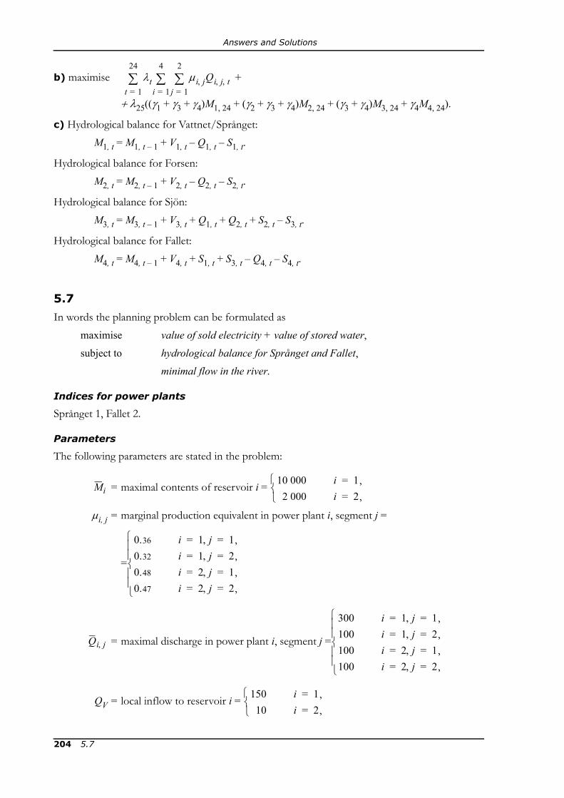
Answers and Solutions
b) maximise +
+ λ25((γ1 + γ3 + γ4)M1, 24 + (γ2 + γ3 + γ4)M2, 24 + (γ3 + γ4)M3, 24 + γ4M4, 24).
c) Hydrological balance for Vattnet/Språnget:M1, t = M1, t – 1 + V1, t – Q1, t – S1, t.
Hydrological balance for Forsen:M2, t = M2, t – 1 + V2, t – Q2, t – S2, t.
Hydrological balance for Sjön:M3, t = M3, t – 1 + V3, t + Q1, t + Q2, t + S2, t – S3, t.
Hydrological balance for Fallet:M4, t = M4, t – 1 + V4, t + S1, t + S3, t – Q4, t – S4, t.
5.7
In words the planning problem can be formulated asmaximise value of sold electricity + value of stored water,subject to hydrological balance for Språnget and Fallet,
minimal flow in the river.
Indices for power plants
Språnget 1, Fallet 2.
Parameters
The following parameters are stated in the problem:
= maximal contents of reservoir i =
μi, j = marginal production equivalent in power plant i, segment j =
=
= maximal discharge in power plant i, segment j =
QV = local inflow to reservoir i =
λt μi j, Qi j t, ,j 1=
2
∑i 1=
4
∑t 1=
24
∑
Mi10 000 i 1,=
2 000 i 2,=⎩⎨⎧
0.36 i 1 j, 1,= =0.32 i 1 j, 2,= =0.48 i 2 j, 1,= =0.47 i 2 j, 2,= =⎩
⎪⎪⎨⎪⎪⎧
Qi j,
300 i 1 j, 1,= =100 i 1 j, 2,= =100 i 2 j, 1,= =100 i 2 j, 2,= =⎩
⎪⎪⎨⎪⎪⎧
150 i 1,=10 i 2,=⎩
⎨⎧
204 5.7

Answers and Solutions
= minimal spillage through the fish ladder of power plant i = 1, i = 1, 2,
= minimal total water flow downstream power plant i = 10, i = 1, 2,λf = expected future electricity price = 185,
λt = expected electricity price during hour t =
The only parameters which have to be calculated are the start contents of the reservoirs:
Mi, 0 = start contents of reservoir i = 0.5 =
Optimisation variables
Qi, j, t = discharge in power plant i, segment j, during hour t, i = 1, 2, j = 1, 2, t = 1, …, 5,
Si, t = spillage from reservoir i during hour t, i = 1, 2, t = 1, …, 5,Mi, t = contents of reservoir i at the end of hour t, i = 1, 2, t = 1, …, 5.
Objective function
maximise + λf((μ1, 1 + μ2, 1)M1, 5 + μ2, 1M2, 5).
Constraints
Hydrological balance for Språnget:M1, t – M1, t – 1 + Q1, 1, t + Q1, 2, t + S1, t = V1, t, t = 1, … 5.
Hydrological balance for Fallet:M2, t – M2, t – 1 + Q2, 1, t + Q2, 2, t + S2, t – Q1, 1, t – Q1, 2, t – S1, t = V2, t, t = 1, … 5.
Minimal flow in the river:
Qi, 1, t + Qi, 2, t + Si, t ≥ i = 1, 2, t = 1, … 5.
Variable limits
0 ≤ Qi, j, t ≤ i = 1, 2, j = 1, 2, t = 1, …, 5,
≤ Si, t, i = 1, 2, t = 1, …, 5,
0 ≤ Mi, t ≤ i = 1, 2, t = 1, …, 5.
5.8
One m3 of the fuel corresponds to 0.4 ton. As the heat content is 5 MWh/ton and the efficiency is40% we get 0,8 MWh electricity per m3 fuel. If the fuel costs 200 ¤/m3 then the variable genera-tion cost is 200/0.8 = 250 ¤/MWh.
Si
Θi
200 t 1,=210 t 2,=210 t 3,=220 t 4,=210 t 5.=⎩
⎪⎪⎨⎪⎪⎧
Mi5 000 i 1,=1 000 i 2.=⎩
⎨⎧
λt μi j, Qi j t, ,j 1=
2
∑i 1=
2
∑t 1=
5
∑
Θi,
Qi j, ,
Si
Mi,
5.8 205

Answers and Solutions
5.9
90 SEK/MWh.
5.10
Cstart-up(1) = 10 000, Cstart-up(2) = 20 000, Cstart-up(3) = 30 000, Cstart-up(4) = 36 820, Cstart-up(5) = 40 566.
5.11
ut – ut – 1 ≤
5.12
In words the planning problem can be formulated asmaximise value of sold electricity – generation costs – start-up costs,subject to limitations in generation capacity,
relation between start-up and unit commitment,requirement on minimum down time in the power plants.
Indices for power plants
Stad I 1, Stad II 2, Stad III 3, Strålinge I 4, Strålinge II 5.
Indices for price areas
Nord 1, Öst 2.
Parameters
The following parameters are stated in the problem:
= installed capacity in power plant g =
= minimal generation when power plant g is committed =
st+.
Gg
200 g 1,=150 g 2,=300 g 3,=600 g 4,=650 g 5,=⎩
⎪⎪⎨⎪⎪⎧
Gg
503080
500500⎩
⎪⎪⎨⎪⎪⎧ g 1,=
g 2,=g 3,=g 4,=g 5,=
206 5.9-5.12

Answers and Solutions
βGg = variable generation cost in power plant g =
= start-up cost in power plant g =
ug, t = commitment of unit g at the beginning of the planning period =
=
λn, t = expected electricity price in area n during hour t =
=
= minimal down time of power plant g = 3, g = 1, …, 5.
Optimisation variables
Gg, t = generation in power plant g, hour t, g = 1, …, 5, t = 1, …, 24,ug, t = unit commitment of power plant g during hour t, g = 1, …, 5, t = 1, …, 24,
= start-up variable for power plant g, hour t, g = 1, …, 5, t = 1, …, 24,= stop variable for power plant g, hour t, g = 1, …, 5, t = 1, …, 24.
Objective function
maximise
Constraints
Maximal generation:
Gg, t – ug, t ≤ 0, g = 1, …, 5, t = 1, …, 24.
150180160100100⎩
⎪⎪⎨⎪⎪⎧ g 1,=
g 2,=g 3,=g 4,=g 5,=
Cg+
20 00018 00032 00040 00040 000⎩
⎪⎪⎨⎪⎪⎧ g 1,=
g 2,=g 3,=g 4,=g 5,=
01⎩
⎨⎧ g 1 2 3, t, , 1 0,,–= =
g 4 5, t, 1 0,,–= =
116118108115160130210136290148⎩
⎪⎪⎪⎪⎪⎪⎪⎨⎪⎪⎪⎪⎪⎪⎪⎧ n 1 2, t, 1,= =
n 1 2, t, 2,= =n 1 2, t, 3 4,,= =n 1 2, t, 5,= =n 1, t 6,= =n 2, t 6,= =n 1, t 7,= =n 2, t 7,= =n 1, t 8,= =n 2, t 8,= =
291148150290145273141272163139
n 1, t 9 10,,= =n 1, t 9,= =n 2, t 10,= =n 1, t 11,= =n 2, t 11,= =n 1, t 12,= =n 2, t 12 13,,= =n 1, t 13,= =n 1, t 14,= =n 2, t 14,= =
138137140142137134130120
98105
n 1 2, t, 15,= =n 1 2, t, 16,= =n 1 2, t, 17,= =n 1 2, t, 18,= =n 1 2, t, 19,= =n 1 2, t, 20,= =n 1 2, t, 21,= =n 1 2, t, 22,= =n 1 2, t, 23,= =n 1 2, t, 24,= =
tg–
sg t,+
sg t,–
λ1 t, Gg t, λ2 t, Gg t,g 4=
5
∑+g 1=
3
∑⎝ ⎠⎜ ⎟⎛ ⎞
βGgGg t, Cg+sg t,
++( ).g 1=
5
∑t 1=
24
∑–t 1=
24
∑
Gg
5.12 207

Answers and Solutions
Minimal generation:
ug, t – Gg, t ≤ 0, g = 1, …, 5, t = 1, …, 24.
Relation between start-up, stop and unit commitment:
ug, t – ug, t – 1 – + = 0, g = 1, …, 5, t = 1, …, 24.
Requirement on down time:
≤ 1, g = 1, …, 5, t = 1, …, 22,
+ ≤ 1, g = 1, …, 5, t = 23.
Variable limits
ug, t ∈ {0, 1}, g = 1, …, 5, t = 1, …, 24,
∈ {0, 1}, g = 1, …, 5, t = 1, …, 24,
∈ {0, 1}, g = 1, …, 5, t = 1, …, 24.
5.13
In words the planning problem can be formulated asmaximise value of stored water – generation costs – start-up costs,subject to hydrological balance for Forsen, Ån and Strömmen,
limitations in generation capacity,
relation between start-up and unit commitment in Viken,delivery of contracted load,limitations in daily carbon dioxide emissions.
Indices of hydro power plants
Forsen 1, Ån 2, Strömmen 3.
Parameters
The following parameters are stated in the problem:μi, j = marginal production equivalent in power plant i, segment j =
=
Gg
sg t,+ sg t,
–
sg t,– sg k,
+
k t 1+=
t tg– 1–+
∑+
sg t,– sg t 1+,
+
sg t,+
sg t,–
0,28 i 1 j, 1,= =0,21 i 1 j, 2,= =0,42 i 2 j, 1,= =0,32
0,34
0,48
i 2 j, 2,= =i 3 j, 1,= =i 3 j, 1,= =⎩
⎪⎪⎪⎨⎪⎪⎪⎧
208 5.13
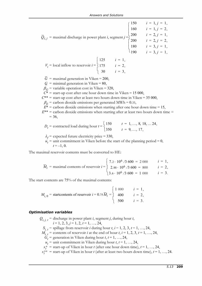
Answers and Solutions
= maximal discharge in power plant i, segment j =
Vi = local inflow to reservoir i =
= maximal generation in Viken = 200,= minimal generation in Viken = 80,
βG = variable operation cost in Viken = 320,C* = start-up cost after one hour down time in Viken = 15 000,
C** = start-up cost after at least two hours down time in Viken = 35 000,βE = carbon dioxide emissions per generated MWh = 0.33,E* = carbon dioxide emissions when starting after one hour down time = 15,
E** = carbon dioxide emissions when starting after at least two hours down time == 36,
Dt = contracted load during hour t =
λf = expected future electricity price = 330,ut = unit commitment in Viken before the start of the planning period = 0,
t = –1, 0.The maximal reservoir contents must be converted to HE:
= maximal contents of reservoir i =
The start contents are 75% of the maximal contents:
Mi, 0 = startcontents of reservoir i = 0.75 =
Optimisation variables
Qi, j, t = discharge in power plant i, segment j, during hour t, i = 1, 2, 3, j = 1, 2, t = 1, …, 24,
Si, t = spillage from reservoir i during hour t, i = 1, 2, 3, t = 1, …, 24,Mi, t = contents of reservoir i at the end of hour t, i = 1, 2, 3, t = 1, …, 24,
Gt = generation in Viken during hour t, t = 1, …, 24,ut = unit commitment in Viken during hour t, t = 1, …, 24,
= start-up of Viken in hour t (after one hour down time), t = 1, …, 24,= start-up of Viken in hour t (after at least two hours down time), t = 1, …, 24.
Qi j,
150 i 1 j, 1,= =160 i 1 j, 2,= =200 i 2 j, 1,= =200180190
i 2 j, 2,= =i 3 j, 1,= =i 3 j, 1,= =⎩
⎪⎪⎪⎨⎪⎪⎪⎧
125175
30⎩⎪⎨⎪⎧ i 1,=
i 2,=i 3,=
GG
150350⎩
⎨⎧ t 1 … 8 18 …24,, , , ,=
t 9 … 17,, ,=
Mi
7.2 106 3 600⁄⋅ 2 000=2.88 106 3 600⁄⋅ 800=
3.6 106 3 600⁄⋅ 1 000=⎩⎪⎨⎪⎧ i 1,=
i 2,=i 3.=
Mi
1 000400500⎩
⎪⎨⎪⎧ i 1,=
i 2,=i 3.=
st*st**
5.13 209
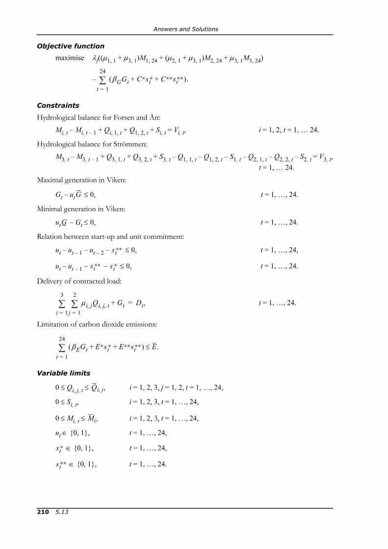
Answers and Solutions
Objective function
maximise λf((μ1, 1 + μ3, 1)M1, 24 + (μ2, 1 + μ3, 1)M2, 24 + μ3, 1M3, 24)
–
Constraints
Hydrological balance for Forsen and Ån:Mi, t – Mi, t – 1 + Qi, 1, t + Q1, 2, t + Si, t = Vi, t, i = 1, 2, t = 1, … 24.
Hydrological balance for Strömmen:M3, t – M3, t – 1 + Q3, 1, t + Q3, 2, t + S3, t – Q1, 1, t – Q1, 2, t – S1, t – Q2, 1, t – Q2, 2, t – S2, t = V3, t,
t = 1, … 24.Maximal generation in Viken:
Gt – ut ≤ 0, t = 1, …, 24.
Minimal generation in Viken:
ut – Gt ≤ 0, t = 1, …, 24.
Relation between start-up and unit commitment:
ut – ut – 1 – ut – 2 – ≤ 0, t = 1, …, 24,
ut – ut – 1 – – ≤ 0, t = 1, …, 24.
Delivery of contracted load:
t = 1, …, 24.
Limitation of carbon dioxide emissions:
Variable limits
0 ≤ Qi, j, t ≤ i = 1, 2, 3, j = 1, 2, t = 1, …, 24,
0 ≤ Si, t, i = 1, 2, 3, t = 1, …, 24,
0 ≤ Mi, t ≤ i = 1, 2, 3, t = 1, …, 24,
ut ∈ {0, 1}, t = 1, …, 24,
∈ {0, 1}, t = 1, …, 24,
∈ {0, 1}, t = 1, …, 24.
βGGt C*st* C**st**++( ).t 1=
24
∑
G
G
st**
st** st*
μi j, Qi j t, , Gt+j 1=
2
∑i 1=
3
∑ Dt,=
βEGt E*st* E**st**++( ) E.≤t 1=
24
∑
Qi j, ,
Mi,
st*
st**
210 5.13
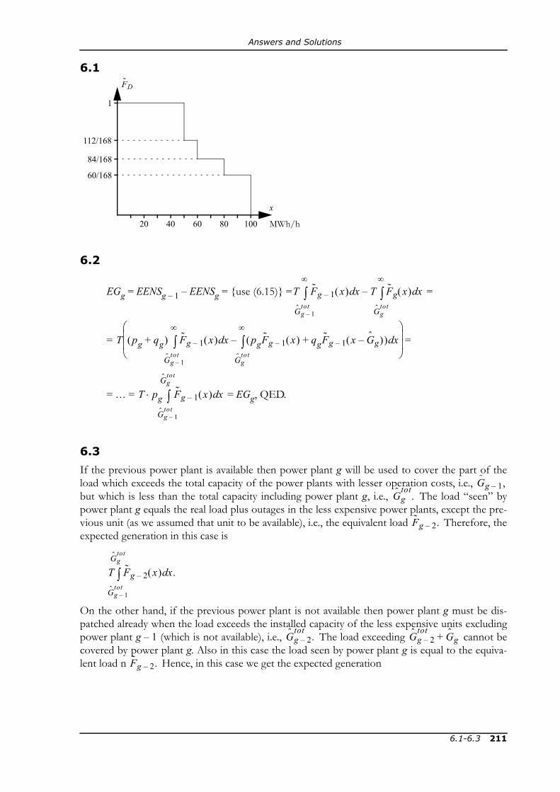
Answers and Solutions
6.1
6.2
EGg = EENSg – 1 – EENSg = {use (6.15)} = =
= =
= … = = EGg, QED.
6.3
If the previous power plant is available then power plant g will be used to cover the part of theload which exceeds the total capacity of the power plants with lesser operation costs, i.e., but which is less than the total capacity including power plant g, i.e., The load “seen” bypower plant g equals the real load plus outages in the less expensive power plants, except the pre-vious unit (as we assumed that unit to be available), i.e., the equivalent load Therefore, theexpected generation in this case is
On the other hand, if the previous power plant is not available then power plant g must be dis-patched already when the load exceeds the installed capacity of the less expensive units excludingpower plant g – 1 (which is not available), i.e., The load exceeding cannot becovered by power plant g. Also in this case the load seen by power plant g is equal to the equiva-lent load n Hence, in this case we get the expected generation
40 MWh/h
x
20 60 80 100
FD
1
112/168
84/168
60/168
T Fg 1– x( ) x T Fg x( ) xd
Ggtot
∞
∫–d
Gg 1–tot
∞
∫
T pg qg+( ) Fg 1– x( ) x pgFg 1– x( ) qgFg 1– x Gg–( )+( ) xd
Ggtot
∞
∫–d
Gg 1–tot
∞
∫⎝ ⎠⎜ ⎟⎜ ⎟⎛ ⎞
T pg Fg 1– x( ) xd
Gg 1–tot
Ggtot
∫⋅
Gg 1– ,Gg
tot.
Fg 2– .
T Fg 2– x( ) x.d
Gg 1–tot
Ggtot
∫
Gg 2–tot
. Gg 2–tot
Gg+
Fg 2– .
6.1-6.3 211

Answers and Solutions
This expression can be simplified by adding to both the upper and lower limit of the inte-gral, while subtracting the same amount from the integration variable. This yields
The expected generation in power plant g is the sum of the generation in the two cases describedabove. If we consider the probability of each case then we obtain the following expression for thetotal expected generation:
EGg = =
=
The function to be integrated is clearly on the same form as the right hand side of (6.13). Hence,the formula above can be simplified to
EGg =
which is the formula we should derive.
6.4
Since we do not know the number and duration of each failure we cannot calculate the MTTF.However, the table shows the sums
= 667.5 + 651 + 633 + 706 = 2 657.5 h
and
= 76.5 + 21 + 111 + 14 = 222.5 h.
This is enough estimation to estimate the availability using the expression
T Fg 2– x( ) x.d
Gg 2–tot
Gg 2–tot
Gg+
∫
Gg 1–
T Fg 2– x Gg 1––( ) x.d
Gg 1–tot
Ggtot
∫
T pg pg 1– Fg 2– x( ) x qg 1– Fg 2– x( ) xd
Gg 1–tot
Ggtot
∫+d
Gg 1–tot
Ggtot
∫⎝ ⎠⎜ ⎟⎜ ⎟⎛ ⎞
⋅
T pg pg 1– Fg 2– x( ) qg 1– Fg 2– x Gg 1––( )+( ) x.d
Gg 1–tot
Ggtot
∫⋅
T pg Fg 1– x( ) x,d
Gg 1–tot
Ggtot
∫⋅
tu k( )k 1=
M
∑
td k( )k 1=
M
∑
212 6.4
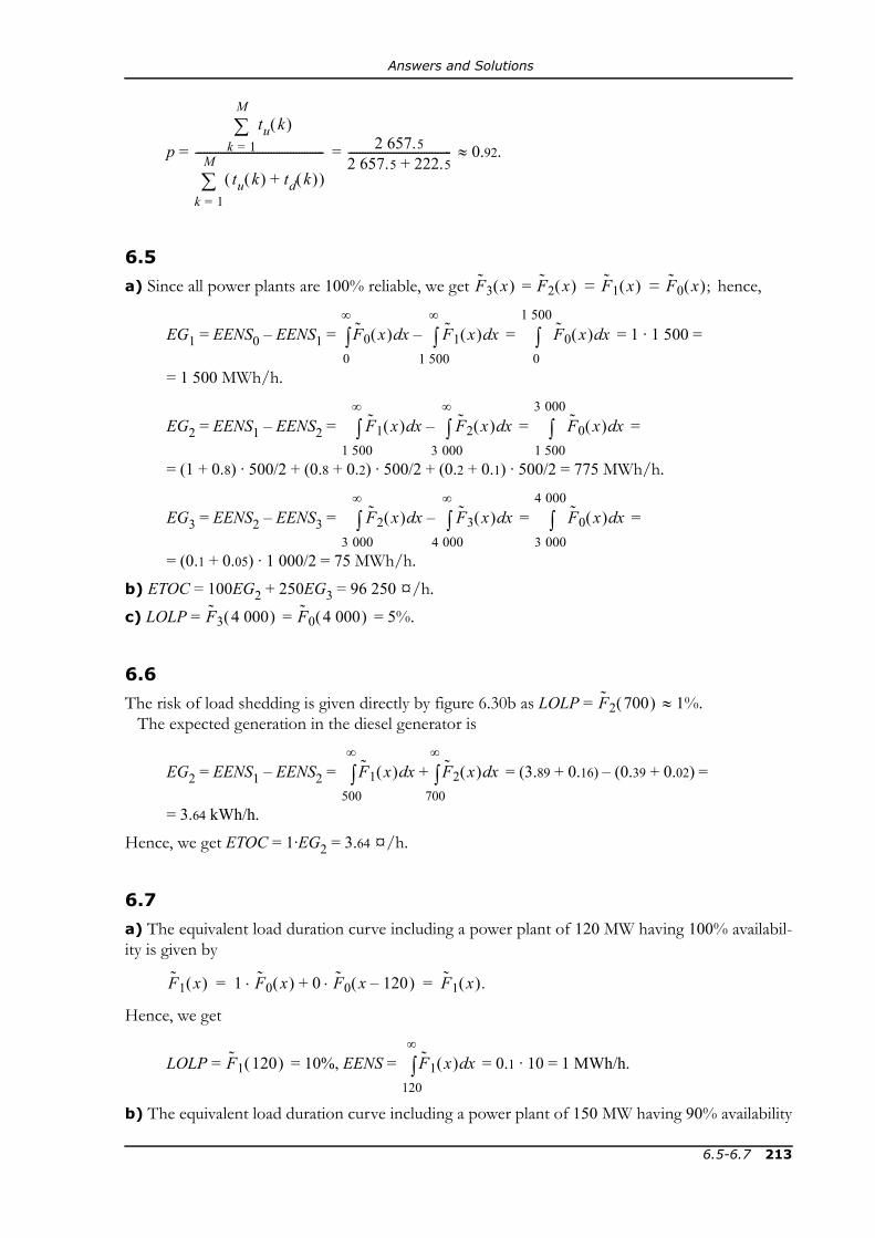
Answers and Solutions
p = = ≈ 0.92.
6.5
a) Since all power plants are 100% reliable, we get = = = hence,
EG1 = EENS0 – EENS1 = = = 1 · 1 500 =
= 1 500 MWh/h.
EG2 = EENS1 – EENS2 = = =
= (1 + 0.8) · 500/2 + (0.8 + 0.2) · 500/2 + (0.2 + 0.1) · 500/2 = 775 MWh/h.
EG3 = EENS2 – EENS3 = = =
= (0.1 + 0.05) · 1 000/2 = 75 MWh/h.b) ETOC = 100EG2 + 250EG3 = 96 250 ¤/h.c) LOLP = = = 5%.
6.6
The risk of load shedding is given directly by figure 6.30b as LOLP = ≈ 1%.The expected generation in the diesel generator is
EG2 = EENS1 – EENS2 = = (3.89 + 0.16) – (0.39 + 0.02) =
= 3.64 kWh/h.Hence, we get ETOC = 1·EG2 = 3.64 ¤/h.
6.7
a) The equivalent load duration curve including a power plant of 120 MW having 100% availabil-ity is given by
Hence, we get
LOLP = = 10%, EENS = = 0.1 · 10 = 1 MWh/h.
b) The equivalent load duration curve including a power plant of 150 MW having 90% availability
tu k( )k 1=
M
∑
tu k( ) td k( )+( )k 1=
M
∑---------------------------------------------- 2 657.5
2 657.5 222.5+-------------------------------------
F3 x( ) F2 x( ) F1 x( ) F0 x( );
F0 x( ) xd0
∞
∫ F1 x( ) xd1 500
∞
∫– F0 x( ) xd0
1 500
∫
F1 x( ) xd1 500
∞
∫ F2 x( ) xd3 000
∞
∫– F0 x( ) xd1 500
3 000
∫
F2 x( ) xd3 000
∞
∫ F3 x( ) xd4 000
∞
∫– F0 x( ) xd3 000
4 000
∫
F3 4 000( ) F0 4 000( )
F2 700( )
F1 x( ) x F2 x( ) xd700
∞
∫+d500
∞
∫
F1 x( ) 1 F0 x( ) 0 F0 x 120–( )⋅+⋅ F1 x( ).= =
F1 120( ) F1 x( ) xd120
∞
∫
6.5-6.7 213
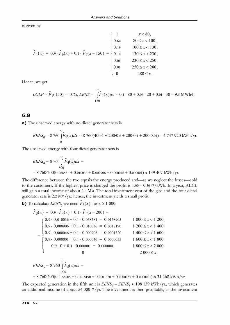
Answers and Solutions
is given by
Hence, we get
LOLP = = 10%, EENS = = 0.1 · 80 + 0.06 · 20 + 0.01 · 30 = 9.5 MWh/h.
6.8
a) The unserved energy with no diesel generator sets is
EENS0 = = 8 760(400·1 + 200·0.6 + 200·0.1 + 200·0.01) = 4 747 920 kWh/yr.
The unserved energy with four diesel generator sets is
EENS4 = =
= 8 760·200(0.068581 + 0.010036 + 0.000906 + 0.000046 + 0.000001) ≈ 139 407 kWh/yr.The difference between the two equals the energy produced and—as we neglect the losses—soldto the customers. If the highest price is charged the profit is 1.00 – 0.50 ¤/kWh. In a year, AECLwill gain a total income of about 2.3 M¤. The total investment cost of the gird and the four dieselgenerator sets is 2.2 M¤/yr.; hence, the investment yields a small profit.b) To calculate EENS5 we need for x ≥ 1 000:
=
EENS5 = =
= 8 760·200(0.0158905 + 0.0018190 + 0.0001320 + 0.0000055 + 0.0000001) ≈ 31 268 kWh/yr.The expected generation in the fifth unit is EENS4 – EENS5 ≈ 108 139 kWh/yr., which generatesan additional income of about 54 000 ¤/yr. The investment is then profitable, as the investment
F1 x( ) 0,9 F0 x( ) 0,1 F0 x 150–( )⋅+⋅
10.64
0.19
0.10
0.06
0.01
0⎩⎪⎪⎪⎪⎨⎪⎪⎪⎪⎧ x 80,<
80 x 100,<≤100 x 130,<≤130 x 230,<≤230 x 250,<≤250 x 280,<≤
280 x.≤
= =
F1 150( ) F1 x( ) xd150
∞
∫
8 760 F0 x( ) xd0
∞
∫
8 760 F4 x( ) xd800
∞
∫
F5 x( )
F5 x( ) 0.9 F4 x( ) 0.1 F4 x 200–( )⋅+⋅=0.9 0,010036 0.1 0.068581⋅+⋅ 0.0158905=0.9 0,000906 0.1 0.010036⋅+⋅ 0.0018190=0.9 0,000046 0.1 0.000906⋅+⋅ 0.0001320=0.9 0,000001 0.1 0.000046⋅+⋅ 0.0000055=
0.9 0 0.1 0.000001⋅+⋅ 0.0000001=0⎩
⎪⎪⎪⎨⎪⎪⎪⎧ 1 000 x 1 200,<≤
1 200 x 1 400,<≤1 400 x 1 600,<≤1 600 x 1 800,<≤1 800 x 2 000,<≤
2 000 x≤ .
=
8 760 F5 x( ) xd1 000
∞
∫
214 6.8
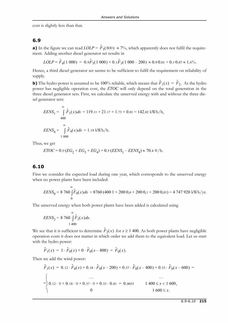
Answers and Solutions
cost is slightly less than that.
6.9
a) In the figure we can read LOLP = ≈ 7%, which apparently does not fulfil the require-ment. Adding another diesel generator set results in
LOLP = ≈ 0.9·0.01 + 0.1·0.07 ≈ 1.6%.
Hence, a third diesel generator set seems to be sufficient to fulfil the requirement on reliability ofsupply.b) The hydro power is assumed to be 100% reliable, which means that As the hydropower has negligible operation cost, the ETOC will only depend on the total generation in thethree diesel generator sets. First, we calculate the unserved energy with and without the three die-sel generator sets:
EENS1 = = 119.11 + 21.17 + 1.73 + 0.01 = 142.02 kWh/h,
EENS4 = = 1.19 kWh/h.
Thus, we getETOC = 0.5·(EG2 + EG3 + EG4) = 0.5·(EENS1 – EENS4) ≈ 70.4 ¤/h.
6.10
First we consider the expected load during one year, which corresponds to the unserved energywhen no power plants have been included:
EENS0 = = 8760·(400·1 + 200·0,6 + 200·0,1 + 200·0,01) = 4 747 920 kWh/yr.
The unserved energy when both power plants have been added is calculated using
EENS2 =
We see that it is sufficient to determine for x ≥ 1 400. As both power plants have negligibleoperation costs it does not matter in which order we add them to the equivalent load. Let us startwith the hydro power:
Then we add the wind power:
=
=
F3 800( )
F4 1 000( ) 0.9F3 1 000( ) 0.1F3 1 000 200–( )+=
F1 x( ) F2.=
F1 x( ) xd400
∞
∫
F4 x( ) xd1 000
∞
∫
8 760 F0 x( ) xd0
∞
∫
8 760 F2 x( ) x.d1 400
∞
∫
F2 x( )
F1 x( ) 1 F0 x( ) 0 F0 x 800–( )⋅+⋅ F0 x( ).= =
F1 x( ) 0.12 F0 x( ) 0.18 F0 x 200–( ) 0.37 F0 x 400–( ) 0.33 F0 x 600–( )⋅+⋅+⋅+⋅=
…0.12 0 0.18 0 0.37 0 0.33 0.01⋅+⋅+⋅+⋅ 0.0033=
0⎩⎪⎨⎪⎧ …
1 400 x 1 600,<≤
1 600 x.≤
6.9-6.10 215

Answers and Solutions
We getEENS2 = 8760· 200·0,0033 = 5 782 kWh/yr.
The generation in the two power plants is equal to the difference between EENS0 and EENS2, i.e.,4 742 138 kWh/yr. If all energy is sold for 1 ¤/kWh then the income will be larger than the an-nual cost. The investments seems to be profitable.
6.11
a) According to the problem we have μL = 3 500 and σL = 300. Using the definitions we get thefollowing mean and standard deviation of outages in the nuclear power plants: μO = 0.95·0 +0.05·1 000 = 50 and = 0.95·(0 – 50)2 + 0.05·(1 000 – 50)2 = 47 500. The equivalent load durationcurve including the five nuclear power plants has the mean
μ5 = μL + 5μO = 3 750
and the standard deviation
σ5 = ≈ 572.
The loss of load probability is then
LOLP ≈ = 1 – = 1 – =
= 1 – Φ(2.18) = {use table} = 0.0146.b) With four nuclear power plants and wind power we get an equivalent load duration curve withthe mean
μ4V = μL + 4μO + 0.6V = 3 700 + 0.6V
and the standard deviation
σ4V = =
If the LOLP is to remain unchanged we must have
= Φ(2.18)
⇒
4 000 + V – 3 700 – 0,6V = 2.18 ·
If we take the square of both sides of the equation and rearrange the expression we get
0.11 + 240V – 1 245 878 = 0 ⇒ V ≈ 2 430.
Thus, it is necessary to build about 2 430 MW wind power if the risk of power deficit should bethe same as before.
6.12
ETOC is estimated by mTOC = = 256 ¤/h.
σO2
ρL2 5ρO
2+
F5N 5 1 000⋅( ) Φ5 000 μ5–
σ5-------------------------⎝ ⎠
⎛ ⎞ Φ 5 000 3 750–572
--------------------------------⎝ ⎠⎛ ⎞
σL2 4σO
2 0.1V( )2+ + 280 000 0.01V2+ .
Φ4 000 V μ4V–+
σ4V---------------------------------------⎝ ⎠
⎛ ⎞
280 000 0.01V2+ .
V2
12 000------------ toci
i 1=
2 000
∑
216 6.11-6.12

Answers and Solutions
LOLP is estimated by mLOLO = = 0.8%.
6.13
LOLP is estimated to 0.12%.
6.14
The U(0, 1)-distributed random numbers are transformed to random number with the distribu-tion FY(x) using the inverse transform method, i.e., by calculating Y = The inverse distri-bution function can be found in the figures, which gives the following random numbers and com-plementary random numbers:
D ≈ 360, D* ≈ 620, = 600, = 800.
We get the following samples of TOC and LOLO:
Hence, ETOC is estimated to 242.50 ¤/h and LOLP to 25%.
6.15
ETOC is estimated to about 71.7 ¤/h when using the control variate method.
D TOC LOLO
600 360 180 0600 620 300 1800 360 180 0800 620 310 0
Mean 242,50 0,25
12 000------------ loloi
i 1=
2 000
∑
FY1– U( ).
G G*
500 kWh/h
x
1
0.6
0.4
0.8
F0
U
D
U*
D*
0.2
500 kWh/h
x
1
0.6
0.4
0.8
FG
U
U*0.2
G G*
G
6.13-6.15 217

Answers and Solutions
6.16
a) The maximal losses in this system are obtained when both hydro and wind power generatestheir installed capacity:
L1, 2 = 3·10–5·8002 = 19.2 kW, {800 = installed hydro capacity}
L2, 3 = 8·10–5·(780.8 + 600)2 ≈ 152.5 kW, {720.8 = maximal import from Ekiyira, 600 = installed wind capacity}
Hence, the maximal losses are = 171.7 kW. This means that there are three interesting intervalsfor the load:
b) First, we compute the mean of the observations for each stratum:
= = 0,
= = 0.1758,
= = 1.
The final estimate of LOLP is calculated by weighting the results according to their stratumweights:
LOLP ≈ = 0.9560 · 0 + 0.0332 · 0.1758 + 0.0108 · 1 = 0.0166 ≈ 1.7%.
The estimates of the expected generation in the power plants is calculated in a similar manner:E[H] ≈ 0.9560 · 41 905/110 + 0.0332 · 255 087/330 + 0.0108 · 6 400/8 ≈ 398 kWh/h,E[W] ≈ 0.9560 · 20 548/110 + 0.0332 · 30 982/330 + 0.0108 · 210/8 ≈ 182 kWh/h.
6.17
= 8, = 20, = 20.
6.18
= 22, = 0, = 14.
TOC LOLO
D ≤ 978.3 0 0978.3 < D ≤ 1 150 0 0 or 1
1 150 < D 0 1
L
mLOLO1
1n1----- LOLO1 i,
i 1=
n1
∑= 0110---------
mLOLO2
1n2----- LOLO2 i,
i 1=
n2
∑= 58330---------
mLOLO3
1n3----- LOLO3 i,
i 1=
n3
∑= 88---
ωhmLOLOhh 1=
3
∑
n12 n2
2 n32
n12 n2
2 n32
218 6.16-6.18

INDEX
annuity formula 90availability 103
balance responsibility 9, 17bilateral electricity market 11block bid 12
capacity credit 91capacity limitation 22central dispatch 16centralised electricity market 11combined heat and power 61complementary random number 124, 126, 137condensing power plant 61constraint 155consumer 8, 11control variate 128, 129, 137convolution 186correlation 188correlation coefficient 188covariance 188
demand curve 12, 21density function 185distributed generation 6distribution function 186distribution grid 5down-regulation 15dual variable 73, 164, 166duration curve 186
EENS 89, 96EG 97ENS 89ETOC 88, 97expectation value 187
failure rate 103financial trading 14firm power 14forecast uncertainty 26frequency 36futures 14
gain 37Gaussian distribution 189grid 5
in multi-area model 85in probabilistic production cost simulation 93
grid owner 9
hydro power 47, 48efficiency 47–50forbidden discharge 52–53hydrological coupling 53in probabilistic production cost
simulation 109–111piecewise linear model 50–53short-term planning 55–61value of stored water 54water value 112
inverse transform method 193investment, value of 90
linear programming 156degenerated solution 161dual problem 162flat optimum 161integer solution 167standard form 157unbounded problem 159
loadmodel 86, 98–102
219

Index
price sensitivity 24load shedding 36–37
see also LOLO, LOLPLOLO 88LOLP 88, 96
market power 27mathematical programming 155MILP see linear programming, integer solutionmodel constant 84Monte Carlo simulation 115MTTF 102MTTR 103multi-area model 84–89
Neyman allocation 133non-dispatchable power plant
model 85normal distribution 189, 194nuclear power 61, 62
objective function 155operation cost
see TOC, ETOCoptimisation theory 155options 14
perfect competition 22perfect information 22photovoltaics 85power deficit
see LOLO, LOLPpower pool 11, 12power system 5price area 13price cross 12primary control 35probabilistic production cost simulation 92
calculation of system indices 96, 107convolution formula 96, 107equivalent load 94normal approximation 112–115
probability distribution 185producer 8, 11pseudorandom number 193
random number 193random variable 185real-time balancing market 14repair rate 103reservoir limitation 22, 25, 109–111
result variable 84in multi-area model 88–89
retailer 8, 11risk of power deficit
see LOLP
sample allocation 142–145scenario 83scenario parameter 83
in multi-area model 87, 89season planning 45secondary control 40short-term planning 45simple sampling 116, 121, 137strata tree 138–142stratified sampling 132, 134, 137sub-transmission grid 5supply curve 12, 21synchronous power system 35system index 84
in multi-area model 88–89probabilistic production cost simulation 96
system operator 9
take-and-pay 14thermal power 61, 62
availability 102–104down time 66–67efficiency 61generation changes 67in multi-area model 85short-term planning 68–73start-up costs 63–65unit commitment 68up time 66–67
time deviation 40TOC 88transmission grid 5transmission limitation 22
in multi-area model 85
unavailability 103up-regulation 16
variable limit 155variance 187variance reduction technique 120vertically integrated electricity market 10, 11
wind power 104model 85, 105–107
220