Computational Statistics and Data Analysis 56 (2012) 1511–1527

Contents lists available at SciVerse ScienceDirect

Computational Statistics and Data Analysis

journal homepage: www.elsevier.com/locate/csda

Efficient Bayesian inference for stochastic time-varying copula modelsCarlos Almeida ∗, Claudia CzadoDepartment of Mathematical Statistics, Technische Universität München, Germany

a r t i c l e i n f o

Article history:Received 23 February 2010Received in revised form 26 August 2011Accepted 26 August 2011Available online 10 October 2011

Keywords:Time varying dependenceNon-Gaussian copulasKendall’s τ

Bayesian inferenceMarkov Chain Monte CarloCoarse grid sampler

a b s t r a c t

There is strong empirical evidence that dependence in multivariate financial time seriesvaries over time. To model this effect, a time varying copula class is developed, whichis called the stochastic copula autoregressive (SCAR) model. Dependence at time t ismodeled by a real-valued latent variable,which corresponds to the FisherZ transformationof Kendall’s τ for the chosen copula family. This allows for a common scale so that ageneral range of copula families including the Gaussian, Clayton and Gumbel copulas canbe used and compared in our modeling framework. The inclusion of latent variables makesmaximum likelihood estimation computationally difficult, therefore a Bayesian approach isfollowed. This approach allows the computation of credibility intervals in addition to pointestimates. TwoMarkov ChainMonte Carlo (MCMC) sampling algorithms are proposed. Thefirst one is a naïve approach using Metropolis–Hastings within Gibbs, while the second isa more efficient coarse grid sampler. The performance of these samplers are investigatedin a simulation study and are applied to data involving financial stock indices. It is shownthat time varying dependence is present for this data and can be quantified by estimatingthe underlying time varying Kendall’s τ with point-wise credible intervals.

Crown Copyright© 2011 Published by Elsevier B.V. All rights reserved.

1. Introduction

Since the introduction of copulas by Sklar (1959) as a tool for constructing multivariate distributions they have becomemore and more popular (see for example the books by Joe, 1997 and Nelsen, 2006). In particular, copula models have beenshown to capture asymmetric return dependences in financial time series data and can therefore be used to both estimateand forecast Value-at-Risk(VaR) with a high level of accuracy; see for example Frees and Valdez (1998) and Cherubini et al.(2004).

In suchmodels univariate parametric time series are assumed for eachmargin, while dependence among the error termsis generated by a copulamodel with constant dependent parameter over time. See Bauwens et al. (2006) for a survey of suchmodels. However empirical work shows that the assumption of constant time dependency is not appropriate for many datasets; see for example Erb et al. (1994), Longin and Solnik (1995) and Engle (2002). This insight started a strong interestin copula based models with time varying dependence parameters. Dias and Embrechts (2004) and Manner and Candelon(2007) use a change point approach to identify a change in the copula dependence, while Giacomini et al. (2009) use thelocal change point (LCP) method of Mercurio and Spokoiny (2004).

An empirical illustration of time varying dependence is shown in Fig. 1. Using ARMA(1, 1)+ GARCH(1, 1) with t-studentinnovations filtered log returns of the Dow Jones Industrial (DJI) and NASDAQ from 01/03/2001 to 10/31/2008 Kendall’s τhave been estimated based on centered rolling windows with different lengths. Even for a window with 250 observationssome time variability can be observed.

∗ Correspondence to: Department of Mathematical Statistics, Technische Universität München, Boltzmannstr. 3, D-85747 Garching, Germany.Tel.: +49 89 28917439.

E-mail addresses: calmeida@ma.tum.de (C. Almeida), czado@ma.tum.de (C. Czado).

0167-9473/$ – see front matter Crown Copyright© 2011 Published by Elsevier B.V. All rights reserved.doi:10.1016/j.csda.2011.08.015

1512 C. Almeida, C. Czado / Computational Statistics and Data Analysis 56 (2012) 1511–1527

Fig. 1. Centered rolling windows based estimates of Kendalls’ τ for DJI and NASDAQ from 01/03/2001 to 10/31/2008 after marginal ARMA(1, 1) +GARCH(1, 1) filtering with t-student innovations.

A recent survey of time varying copula models is given byManner and Reznikova (2009). Early time-varying dependencemodels are the DCC models proposed by Tse and Tsui (2002) and Engle (2002), which model conditional correlations. Theyare observation driven and require special efforts to achieve a positive definite correlationmatrix. As noted by Bauwens et al.(2006) a drawback of these DCCmodels is that the parameters needed tomodel time dependences are scalar and thus implythat the conditional correlations between different pairs of variables obey the same nonstochastic dynamics. Additionally,since these models are correlation based they incorporate only dependences allowed by elliptical distributions.

More general are copula-GARCHmodels (Patton, 2006; Jondeau andRockinger, 2006; Bauwens et al., 2006). Thesemodelsassume GARCH margins, while the dependence is modeled by a copula. Estimation is usually carried out in a two stepapproach, since a joint estimation of all parameters is too computationally burdensome. First the marginal parameters areestimated and then these estimates are used to transform the standardized innovations via the probability integral transformto the so called copula data. Finally this copula data is used to estimate the copula parameters. Joe (2005) and Patton (2006)have shown that this leads to consistent, but not efficient estimators, whenmaximum likelihood (ML) estimators are used atthe two estimation steps. Consistency is also achieved if one uses normalized ranks of the standardizedmarginal innovationsto transform to copula data. Liu and Luger (2009) have proposed an algorithm to improve the efficiency in copula-GARCHmodels when ML estimation is used. Subsequent time-varying copula-GARCH models have been suggested by Jondeau andRockinger (2006) and Patton (2006).

As an alternative to GARCH models, stochastic volatility (SV) models (see for example Taylor, 1986) can be used asmarginal models together with a copula to construct multivariate financial time series models. Multivariate generalizationsof the SV model were proposed by Harvey et al. (1994) while Yu and Meyer (2006) considered a bivariate SV model withtime dependent stochastic correlations assuming multivariate normal or t errors. The use of marginal SV models togetherwith an arbitrary bivariate copula family have been investigated by Hafner andManner (2010). They allow for time-varyingstochastic copula parameters by choosing a transformation from the copula parameter space to the real numbers andassuming a Gaussian AR(1) model for the transformed copula parameter. Estimation is facilitated using efficient importancesampling (Liesenfeld and Richard, 2003; Richard and Zhang, 2007), however standard error are difficult to estimate.

In a Bayesian approachusingMarkovChainMonte Carlo (MCMC) algorithms abroad range of inference, including credibleintervals can be obtained in a straightforward manner using samples from the posterior distribution.

This advantage of the Bayesian approach has been recognized by Yu and Meyer (2006) and Ausin and Lopes (2010).However it is challenging to construct and implement MCMC algorithms that are fast and mix well. Yu and Meyer (2006)utilizes one parameter at the time Gibbs sampling for each component of the parameter vector. They contend that thismight not be an efficient way of sampling from the posterior. In contrast Ausin and Lopes (2010) consider a copula-GARCHmodel with the nonstochastic dependence dynamics chosen as in Tse and Tsui (2002). This restricts the class of copulasconsidered to the class of elliptical copulas. Ausin and Lopes (2010) estimate marginal and copula parameters jointly.They use multivariate randomwalk Metropolis–Hastings (MH) updates for the dynamic copula parameters and the GARCHparameters of each margins, respectively. They report that individual random walk MH-updates result in slow mixing ofthe MCMC samples. Their dynamics of the copula parameters is nonstochastic and observation driven, thus BayesianMCMCalgorithms are much simpler.

Our goal is to develop efficient MCMC estimation algorithms for stochastic time-varying copula models. To modelstochastic dynamics, a Gaussian AR(1) model for the inverse Fisher transformation of the Kendall’s τ parametercorresponding to the chosen copula is used. This is in line with the model considered in Hafner and Manner (2010). Thisapproach is valid for any copula specified by a single parameter, and specifically Gaussian, double Clayton and the doubleGumbel copula have been studied. For a definition of double Clayton and double Gumbel, respectively, see Section 4. Thesampling schemes proposed here can be generalized to two-parameter families if the dynamics are clearly specified. Forexample, in a t-copula family, the Kendall’s τ could be time dependent and the degrees of freedom remain constant.However, extra parameters will usually result in slower mixing.

C. Almeida, C. Czado / Computational Statistics and Data Analysis 56 (2012) 1511–1527 1513

To build the sampling scheme, a latent variable approach based on the data augmentation principle of Tanner and Wong(1987) is used. A first naïve Gibbs sampling method for updating the latent variables individually is developed. As expectedthis is not very efficient and the sampler is improved by developing by a coarse grid sampler as introduced by Liu andSabatti (2000). The model is applied to the daily returns of the DJI and the NASDAQ data and interesting empirical resultsare uncovered.

The paper is organized as follows. In Section 2 the proposed stochastic dynamic copula model is introduced andappropriate priors are chosen. In Section 3 expressions for the full conditional densities which are needed for aMetropolis–Hastings within Gibbs sampler are derived. An appropriate coarse grid method for updating the latent variablesis also developed. A large simulation study to investigate the behavior of the MCMC samplers is conducted in Section 4. Anapplication to daily returns of DJI and NASDAQ is presented in Section 5 including an evaluation of the forecast performance.Here we used the continuous rank probability score of Gneiting and Raftery (2007) to assess the quality of forecast. Finally,concluding remarks and an outlook are given in Section 6.

2. Model

Let (y1, y2) ∈ R2 be a bivariate randomvectorwithmarginal cumulative distribution functions (cdfs) Fi, i = 1, 2 and jointcdf H . Using Sklar’s theorem (Sklar, 1959), H can be expressed as H(y1, y2) = C(F1(y1), F2(y2)), where C is a copula cdf. Forabsolutely continuous distributions this can be rewritten for densities as h(y1, y2) = c(F1(y1), F2(y2))f1(F1(y1))f2(F2(y2)),where c is the corresponding copula density.

In financial applications knowledge of the past is collected in the filtration Ft−1 and time series data (y1,t , y2,t) fort = 1, . . . , T is observed. Patton (2006) models the conditional joint distribution of (y1,t , y2,t) given Ft−1 as

Ht(y1,t , y2,t | Ft−1) = C(F1,t(y1,t | Zt−1, β1), F2,t(y2,t | Zt−1, β2) | Zt−1, α).

Here Zt−1 is a set of variables in Ft−1, while βi, i = 1, 2 are parameters for the marginal models and α for the dependencemodel, respectively. It follows immediately that the log-likelihood (L) can be decomposed as follows:

L12(β1, β2, α) = L1(β1)+L2(β2)+LC (β1, β2, α),

which separates the contributions to the joint likelihood (L12) into marginal contributions (Li, i = 1, 2) and the copulacontribution (LC ). This motivates a two stage estimator.

In the first stage the marginal parameters βi, i = 1, 2 are estimated by maximizing over Li(βi) separately, giving βi.For the second stage the dependence parameter α is estimated by maximizing LC (β1, β2, α) over α. This approach is calledinference function for margins or IFM method. It was introduced by Joe (1996) and its consistency was proved in Joe (1997).

Genest et al. (1995) propose a different two step estimator, where themargins are transformed by ranks to copula data inthe first stage. This corresponds to an empirical probability integral transformation. In the second stage only the dependenceparameter α is estimated. This semi-parametric method is also consistent and more robust than the IFM method whenmisspecification of margins is severe (see Kim et al., 2007).

While consistency results are available for a two step approach in the classical setting, this is not the case in a Bayesiansetting. However empirical studies of Czado et al. (2011) for a time constant copula model with AR(1) margins, Ausin andLopes (2010) for a different time varying copula model and Hofmann and Czado (submitted for publication) for a timeconstant copula model with GARCH(1, 1) margins have shown that results do not vary substantially if one ignores theestimation uncertainty of the margins. Therefore we follow a pragmatic view point, where marginal models are fittedindependently and residuals (or fitted innovations) will be considered as ‘‘true’’ observations.

Thus, we focus on building a copula model on [0, 1]2 which allows for time varying dependence. In particular, Fi,t(yi,t |Zt−1, βi) is replaced by Fi,t(yi,t | Zt−1, βi) and is treated as the true observations ui,t = Fi,t(yi,t | Zt−1, βi) for i = 1, 2.

Let ut := (u1,t , u2,t)⊤∈ [0, 1]2: t = 1, . . . , T be a sample such a that

ut | (u1, . . . , ut−1), (θ1, . . . , θt) ∼ Cθt , (1)

where Cθt corresponds to a copula distributionwith time varying parameter θt ∈ Θ ⊂ R. The parameters θt will bemodeledas latent variables where the latent variable θt−1 directly influences only ut−1 and θt as shown in Fig. 2.

This structure implies the following conditional independence conditions:

1. The variables u1, . . . , uT are conditionally independent given the latent variables θ1, . . . , θT , i.e.

p(u1, . . . , uT | θ1, . . . , θT ) =

Tt=1

p(ut | θ1, . . . , θT ). (2)

2. The present observation ut does not depend on the past and future latent variables θ1, . . . , θt−1, θt+1, . . . , θT given thepresent value of the latent variable θt , i.e.

p(ut | θ1, . . . , θT ) = p(ut | θt). (3)

1514 C. Almeida, C. Czado / Computational Statistics and Data Analysis 56 (2012) 1511–1527

Fig. 2. Assumed time dependence between u1, . . . , uT induced through latent variables θ1, . . . , θT (arrows indicate dependence).

This structure potentially excludes some interesting cases. For example consider two nonsimultaneous traded indices,such asDAX (Deutscher Aktien IndeX) versusDJI. The closingDJI value at day t hasmore influence on theDAX closing value atday t + 1 compared to the one at time t , since there are only few common open trading hours. This suggests a dependencedescribed by: p(ut | u1, . . . , ut−1, θ1, . . . , θt) in (2). However, this makes the computation infeasible and might involvesome identifiability issues.

The fact that the parameters of the different copula families have different domains, motivates a reparametrizationto a common domain that allows dependence to be compared across copula families. From the literature on copulas, agenerally accepted measure of dependence is the Kendall’s τ coefficient. Most bivariate copula families have a one-to-one transformation from the parameter space Θ into the range corresponding Kendall’s τ values, which we denote byτt := τ(θt).

In our examples, wewill consider only bivariate copulas where the range of possible Kendall’s τ values is in the completeinterval [−1, 1]. This includes the Gaussian copula

τ(θt) =

2πsin−1(θt)

, but not the standard Clayton

τ(θt) =

θ2+θ

> 0

and Gumbelτ(θt) =

θθ−1 > 0

. Therefore we use the double Clayton and Gumbel copulas, which also allows for negative

Kendall’s τ . A precise definition is given in Study II of Section 4.We utilize the inverse Fisher Z transformation h from R to (−1, 1) given by τt :=

exp(2γt )−1exp(2γt )+1

=: h(γt).Thus the relationship between the latent variables γt ∈ R and the time varying copula parameter θt is given by

θt = τ−1(τt) = τ−1exp(2γt)− 1exp(2γt)+ 1

. (4)

Since we require (−1, 1) to be the range of possible Kendall’s τ(θt) values, the relationship between γt and θt is one-to-one.We now specify a stochastic time series model for γt . Possible choices are randomwalk, an autoregressive model or even

a regime switching model for γt . To avoid non-stationarity and enforce parsimony we select the stationary AR(1) model forγt . This also allows comparison to the model proposed in Hafner and Manner (2010), whose parameters are estimated in aclassical framework. More precisely, we assume

γt = µ+ φ(γt−1 − µ)+ σεt for t = 2, . . . , T ,

γ1 ∼ N

µ,σ 2

1− φ2

,

(5)

where εt ∼ N(0, 1) i.i.d. and N(a, b2) denotes a normal distribution with mean a and variance b2. To enforce stationarity,the copula dependence parameter vector α = (µ, φ, σ 2) is in R× (−1, 1)×R+. Further we call the model specified by (1)and (5) a stochastic copula autoregressive (SCAR) model and denote it by SCAR(µ, φ, σ 2).

Stationarity in (5) enforces the copula parameter to return to a conditional mean depending solely on µ. In the randomwalk case (φ = 1) µ is not identified, therefore this cannot be treated using (5). For the financial data presented later theestimated value of φ was far from 1.Likelihood.

Using x1:N := (x1, . . . , xN)⊤ and assuming the conditions (2) and (3), the joint likelihood of u1:T and γ1:T can beexpressed as:

p(u1:T , γ1:T | α) =

1≤t≤T

p(ut | γt) · p(γ1 | α)

2≤t≤T

p(γt | γt−1, α), (6)

where p(ut | γt) is determined by cθt (ut). More precisely for ut = (u1,t , u2,t)⊤ and using (4) we have:

p(ut | γt) = cθt (u1,t , u2,t), where θt = τ−1(h(γt)). (7)Prior specifications.

For the priors of the copula parameters α = (µ, φ, σ 2) standard priors for AR(1) models are used (see e.g. Chib andGreenberg, 1994). In particular we assume p(α) = p(φ | µ, σ 2)p(µ | σ 2)p(σ 2) with

(a) σ 2∼ IG(a, b),

(b) µ | σ 2∼ N(c, d2),

(c)φ + 1

2| σ 2, µ ∼ Beta(e, f ),

(8)

C. Almeida, C. Czado / Computational Statistics and Data Analysis 56 (2012) 1511–1527 1515

where a, b, c, d2, e and f are known hyper-parameters. Here IG(a, b) denotes the inverse Gamma distribution with density

p(σ 2) = baΓ (a)

1

σ 2

a+1exp

−

bσ 2

and Beta(e, f ) the Beta distributionwith density p(x) = 1

B(e,f )xe−1(1−x)f−1, respectively.

Since the prior for (µ, σ 2) is a conjugate prior for (6) for known φ, the full conditionals for µ and σ 2 are easy to deriveanalytically, while for updating φ we require a Metropolis–Hastings (MH) step. Therefore a MH within Gibbs sampler willbe developed. The values of the hyper-parameters can be chosen to reflect prior information. A reference prior is availableby considering the limiting case when a→ 0, b→ 0, d2 →∞, e→ 1, f → 1 giving p(µ, φ, σ 2) ∝ 1

σ 2 .

3. Posterior inference

In this section MH within Gibbs samplers are developed for the model parameters α and latent variables γ =(γ1, . . . , γT )

⊤ jointly. A first sampler consists of naïvely updating γ individually. A second more efficient sampling schemewill then be developed using ideas of Liu and Sabatti (2000).Updating latent variables γ .

Let γA := (γt : t ∈ A) and γ\A := γAC . Similarly we define uA and u\A. It follows that

p(γA | u1:T , α, γ\A) = p(γA | uA, γ\A, α)

∝ p(uA, γA | γ\A, α)

= p(γA | γ\A, α)p(uA | γA, γ\A, α)

= p(γA | γ\A, α)p(uA | γA) (by (2) and (3)). (9)

Thus, in a blocked Gibbs sampling scheme for updating γA by using p(γA | u1:T , α, γ\A), only the observations included inuA are involved. Consequently some computations are simplified.Naïve method.

The update of the latent variables γ is based on the data augmentation principle of Tanner and Wong (1987). The latentvariables are treated as unknown and therefore simulated from the posterior. The full conditional distributions can bederived as follows.

From (9) it follows for A = {t} that

p(γt | u1:T , γ\t , α) ∝ p(γt | γ\t , α)p(ut | γt). (10)

The Gaussian AR(1) specification for γt , given in (5), implies:

γt | γ\t , α ∼ N(γ ∗t , σ ∗t2), (11)

where

γ ∗1 := µ+ φ(γ2 − µ), σ ∗12:= σ 2,

γ ∗t := µ+φ

1+ φ2(γt+1 + γt−1 − 2µ), σ ∗t

2:=

σ 2

1+ φ2, for t = 2, . . . , T − 1,

γ ∗T := µ+ φ(γT−1 − µ), σ ∗T2:= σ 2.

Thus, in order to update γt given u1:T , γ\t , α, we perform a Metropolis–Hasting (MH) step for γt with proposal density

N(γ ∗t , σ ∗t2) and MH-ratio given by: min

p(ut |γt )p(ut |γt )

, 1

, where γt is the proposal value and γt the current value. For moredetails see Algorithm 1 in Appendix A.

Despite its generality and easy implementation, this updating procedure has drawbacks. It shows poor convergence andmixing. One reason for this could be that the proposal density is far from the posterior one. Improvementswill depend on thefunctional form of the selected copula family. For example Geweke and Tanizaki (2001) suggest different proposal densitieswhich depend on approximations of posterior densities or at least on approximations of the first and second moments.However, we will follow a different way of improving the mixing of the MCMC algorithm. In the naïve method, the latentvariables are updated individually taking into account the autoregressive structure of the latent variables. Therefore wesuggest to extend the single updating step to updating steps for neighborhoods.Coarse grid (CG) method.

The basis of this method can be found in Liu and Sabatti (2000). It requires more computational effort, but the behaviorof the simulated Markov chain is improved significantly.

The general idea of the CG method is to find a group of random transformations which leaves the distribution such asthe posterior or the full conditional distribution invariant. Here we choose the full conditional distribution of γ1:T , since theautoregressive structure implies slowmixing of this full conditional. These random transformations are then applied to thenaïve sample. Motivated by Example 4.1 of Liu and Sabatti (2000), we consider for each t = 1, . . . , T the following group oftransformations:

Γt := {gt : gt(γ1:T ) = γ1:T + λtbt}, (12)

1516 C. Almeida, C. Czado / Computational Statistics and Data Analysis 56 (2012) 1511–1527

where bt ∈ RT is fixed, and λt ∈ R. Even though bt can be chosen arbitrarily, a convenient choice incorporates somecharacteristics of the Markovian structure. As in Liu and Sabatti (2000) we use:

b1 =

1,

φ

1+ φ2, 0, . . . , 0

⊤,

b2 =

φ, 1,

φ

1+ φ2, 0, . . . , 0

⊤,

bt =

0, . . . , 0,

φ

1+ φ2, 1,

φ

1+ φ2, 0, . . . , 0

⊤for t = 3, . . . , T − 2,

bT−1 =

0, . . . , 0,

φ

1+ φ2, 1, φ

⊤and

bT =

0, . . . , 0,

φ

1+ φ2, 1⊤

,

(13)

which corresponds to transform (γt−1, γt , γt+1) intoγt−1 +

φλt1+φ2 , γt + λt , γt+1 +

φλt1+φ2

, for t = 3, . . . , T − 2. The group

of transformations given in (12) and (13) satisfies the condition of Theorem 1 in Liu and Sabatti (2000). Therefore the densityp(λt | u1:T , γ1:T , α) of the random transformation λt which leaves the conditional distribution p(γ1:T | u1:T , α) invariant isproportional to

p(λt | u1:T , γ1:T , α) ∝ p(gt(γ1:T ) | u1:T , α) · |Jgt (γ1:T )| · Lt(dλt). (14)

Here Jgt (γ1:T ) is the Jacobian matrix of the transformation and Lt is the left Haar invariant measure associated to the groupof transformations Γt . Is easy to verify that |Jλt (γ1:T )| = 1 and that Lt is the Lebesgue measure.

From the general model specification, and using the Bayes’ Theorem together with using (2) and (3), the full conditionalcan be expressed as

p(γ1:T | α, u1:T ) ∝ p(u1:T | γ1:T , α)p(γ1:T | α)

= p(u1:T | γ1:T )p(γ1:T | α).

Denoting by RT ∈ RT×T the matrix with (i, j)-th element given by φ|i−j|, 1 ≤ i, j ≤ T , it follows from the AR(1)specification in (5) that

γ1:T | α ∼ NT

1Tµ,

σ 2

1− φ2RT

, (15)

which implies that

p(γ1:T | α) ∝ exp−

1− φ2

2 σ 2(γ1:T − 1Tµ)⊤R−1T (γ1:T − 1Tµ)

.

This yields

p(gt(γ1:T )|α) ∝ exp−

1− φ2

2σ 2(γ1:T + λtbt − 1Tµ)⊤R−1T (γ1:T + λtbt − 1Tµ)

.

Using (14) it follows that

p(λt | γ1:T , u1:T , α) ∝ exp−

1− φ2

2σ 2(γ1:T + λtbt − 1Tµ)⊤R−1T (γ1:T + λtbt − 1Tµ)

· p(u1:T | gt(γ1:T ))

= exp−

1− φ2

2 σ 2(λ2

t b⊤

t R−1T bt)+ 2(γ1:T − 1Tµ)⊤R−1T btλt

· p(u1:T | gt(γ1:T ))

∝ exp

− (1− φ2)b⊤t R−1T bt

2σ 2

λt +

(γ1:T − 1Tµ)⊤R−1T bt

b⊤t R−1T bt

2 · p(u1:T | gt(γ1:T ))

= exp−

1

2V ∗t2 (λt − λ∗t )

2· p(u1:T | gt(γ1:T )) (16)

with

λ∗t := −(γ1:T − 1Tµ)⊤R−1T bt

b⊤t R−1T bt

and V ∗t2:=

σ 2

(1− φ2)b⊤t R−1t bt

. (17)

C. Almeida, C. Czado / Computational Statistics and Data Analysis 56 (2012) 1511–1527 1517

Now, by applying Eq. (16), we can show that, for all a ∈ Rp(λt | γ1:T , u1:T , α) = p(λt + a | γ1:T − a1T , u1:T , α) holds. Thiscorresponds to the transformation-invariant property (1) of Liu and Sabatti (2000). Therefore we can apply Theorem 2 ofLiu and Sabatti (2000) and use MH steps for updating λt . Therefore, we sample λt derived from a MH step with proposaldistribution N(λ∗t , V

∗t2) and MH-ratio

minp(uAt | γAt + λtbAt )

p(uAt | γAt ), 1

, (18)

where At = {j ∈ {1, . . . , T }: bt,j = 0} and bt,j is the jth component of bt .In summary, the complete coarse grid update proceeds as follows:

• For current values of α update γ1:T using the naïve method.• For t = 1, . . . , T , simulate a λt by using MH step as described in (18), compute gt(γ1:T ) = γ1:T + λtbt and use them as

new values for γ1:T .

The MH-ratio in (18) can be computed quickly. This is due to the large number of zeros in bt (the cardinality of At is twoor three). Further terms in the likelihood concerning u\At cancel out in the ratio due to conditional independences. Moredetails are given in Algorithm 2 in Appendix A. In Appendix B we provide simple equations for determining λ∗t and V ∗t

2.For the future, different transformations could be considered, a possibility is to use a different set of vectors {bt : t =

1, . . . , T } but a careful check of the invariant property (Condition 1 from Liu and Sabatti, 2000) needs to be conducted;additionally the computational cost needs to be considered.Updating model parameters α of the latent variables.

The conditional independence conditions imply that once the latent variables are updated, the new values for theparameters µ, φ, σ 2 depend only on the current values of the latent variables γ1:T and not on the observed values u1:T ,i.e.

p(µ, φ, σ 2| γ1:T , u1:T ) = p(µ, φ, σ | γ1:T ). (19)

Therefore, by using the conjugacy of the chosen prior, the full conditional distributions of µ and σ 2 are given by:

σ 2| µ, φ, γ1:T , u1:T ∼ IG(a, b) and (20)

µ | σ 2, φ, γ1:T , u1:T ∼ N(c, d2), (21)

where a := a+ T2 , b := b+ 1

2

Tt=2(γt − µ− φ(γt−1 − µ))2 + (1− φ2)(γ1 − µ)2

, d2 :=

1d2+

(T−1)(1−φ)2+(1−φ2)2

and

c := d2

cd2+

1σ 2

(1− φ2)γ1 +

Tt=2(γt − φγt−1)

. For φ, the full conditional density is given by:

p(φ | µ, σ 2, γ1:T , u1:T ) ∝ (1+ φ)e−12 (1− φ)f−

12 ϕ

φ;

S1S0

,σ 2

S0

1[−1,1](φ), (22)

where ϕ(·;µ, σ 2) is the normal densitywithmeanµ and variance σ 2, S0 :=T−1

t=2 (γt−µ)2 and S1 :=T

t=2(γt−µ)(γt−1−

µ). Therefore a MH-step is carried out using a truncated normal as proposal, which is corrected by using the remainingfactors. Algorithm 3 in Appendix A summarizes the updating of the latent model parameters. We remark that the derivationof the full conditionals follows the same development as in Chib and Greenberg (1994) except for a modification in the fullconditional of φ, where a different prior was chosen.

4. Simulation studies

Two studies are conducted, the first one investigates the accuracy of the CG sampler as the sample size increases, whilethe second one studies and compares the performance of the two samplers under different copulas.Study I (Small sample performance of the CG sampler for a Gaussian SCAR (µ, φ, σ 2)).

For this study we simulate from a Gaussian-SCAR(0.5, 0.9, .152) model with different sample sizes, i.e. the dependenceis described by a Gaussian copula, and the parameters of the AR(1) latent process are µ = 0.5, φ = 0.9 and σ 2

= 0.152.For each sample size T = 100+ 10 i; i = 0, . . . , 200 a Markov chain has been simulated by using the CG sampler and 90%credible intervals have been estimated based on 100000 iterates with a thinning of 10. The panels in Fig. 3 show that thecredibility intervals contain the true values and they become smaller when the sample size increases.

To gain more insight into the behavior of the CG sampler the results of a single CG run using 100000 iterations with athinning of 10 for a single Gaussian SCAR data set of T = 2000 is shown in Fig. 4. We see that the posterior mode estimatesare not too far from the true values.

In a bivariate Gaussian copula model with parameter θ we can express Kendall’s τ as τ = 12 sin−1(θ). Therefore we

use the latent MCMC iterates for γt together with (4) to construct posterior mean estimates and credible intervals for thecorresponding time varying Kendall’s τt pointwise. Fig. 5 shows posterior mean estimates (solid line) and 90% credible

1518 C. Almeida, C. Czado / Computational Statistics and Data Analysis 56 (2012) 1511–1527

Fig. 3. Estimated 90% credibility intervals (dotted lines) together with posterior mean estimates (solid line) for the parameters of a Gaussian-SCAR(0.5, 0.9, 0.15), as sample size T increases using the CG sampler. The horizontal line indicates the true parameter values.

0.7

0.5

0.3

0 20000 60000

0 20000 60000

0 20000 60000

0.84

0.90

0.94

0.10

0.16

0.8

0.4

0.0

0.8

0.4

0.0

0.8

0.4

0.0

0 10 20 30 40 50

0 10 20 30 40 50

0 10 20 30 40 50

02

46

80

1020

010

2030

0.3 0.4 0.5 0.6 0.7

0.84 0.88 0.92 0.96

0.10 0.12 0.14 0.16 0.18 0.20

Fig. 4. MCMC traces (left column), estimated autocorrelations of MCMC iterates (middle column) and posterior density estimates (right column) for µ

(top row), φ (middle row) and σ (bottom row) using a CG sampler for a sample from a Gaussian-SCAR(0.5, 0.9, 0.152) of size T = 2000 (– posterior modeestimates, – true values).

intervals for τt based on the CG sampler using the Gaussian SCAR(0.5, 0.9, 0.152) sample of T = 1000 for the last 200observations. It shows that the true τt values (dotted lines) are well covered. Furthermore we see wider credible intervalsfor lower values of τt compared to higher values. This is due to the fact that an observation (u1,t , u2,t) where u1,t ≈ u2,t canbe associated with high dependence but also with low dependence, while an observation where u1,t ≪ u2,t or u1,t ≫ u2,tcan only be associated with lower dependence. Thus low values of the Kendall’ τ , i.e. lower dependence, are less preciselyestimated. Additionallywe see that the credible intervals are nonsymmetric, reflectingnonsymmetric posterior distributionsof τt .Study II (Comparing of coarse grid and naïve sampler under several copula SCAR(µ, φ, σ 2) models).

In this study we fix the sample size to T = 1000 and generate 100000 MCMC iterations for the naïve (N) and forCG sampler, respectively, for each data set. Data sets are generated from Gaussian, double Clayton and double GumbelSCAR(µ, φ, σ 2) models.

The definition of a double Clayton is as follows: Denoting by C(θ) a Clayton copula with parameter θ ∈ [0,∞). A randomvector (U, V ) ∈ [0, 1]2 is distributed as a double Clayton with θ ∈ R if (U, V ) is distributed as a Clayton C(θ) for θ ≥ 0and (U, 1− V ) is distributed as a Clayton C(−θ) for θ < 0. The copula for θ < 0 can also be viewed as a rotated copula by90°. This idea can be applied to other copula families such as the Gumbel copula and further examples can be found in Joe(1997).

The motivation for using these copulas rather than a simple Clayton or Gumbel is to avoid problems when negativedependence estimates occurs. This could happen if τt is negatively estimated for some MCMC iterations. Even if negativedependence is not present in the data, we will expect at most a few negative τt iterations. This approach permits us to use

C. Almeida, C. Czado / Computational Statistics and Data Analysis 56 (2012) 1511–1527 1519

Fig. 5. Estimated posterior Kendall’s τt for the last 200 observations from a Gaussian-SCAR(0.5, 0.9, 0.152) copula data set of size T = 1000 using the CGsampler with 100000 iterations.

Table 1Estimated relative biaswith estimated standard errors in parentheses and the inefficiency factors of Gaussian SCARmodels. The improvement in percentageof the CG sampler over the N sampler is shown in parentheses.

True values SN Relative bias INEFFµ φ σ µ φ σ µ φ σ

N sampler

0.5 0.5 0.15 2.89 −0.004 (0.004) 0.019 (0.042) −0.104 (0.022) 45.74 296.54 436.380.9 0.5 0.15 5.20 −0.001 (0.002) 0.004 (0.034) −0.030 (0.018) 35.31 184.58 284.140.5 0.8 0.15 2.00 0.001 (0.005) −0.002 (0.006) 0.007 (0.018) 16.84 159.57 274.820.9 0.8 0.15 3.60 −0.004 (0.003) 0.005 (0.006) −0.014 (0.012) 12.42 114.18 184.900.5 0.5 0.10 4.33 0.006 (0.003) −0.156 (0.049) −0.037 (0.023) 72.23 372.83 501.520.9 0.5 0.10 7.79 −0.002 (0.002) −0.088 (0.038) −0.011 (0.020) 59.07 292.00 395.590.5 0.8 0.10 3.00 0.008 (0.004) −0.058 (0.021) 0.047 (0.025) 41.28 345.24 478.990.9 0.8 0.10 5.40 −0.006 (0.002) −0.029 (0.010) 0.045 (0.021) 31.19 239.08 360.840.5 0.0 0.15 3.33 −0.004 (0.003) – −0.151 (0.022) 78.02 339.51 474.08

CG sampler

0.5 0.5 0.15 2.89 −0.001 (0.004) −0.093 (0.038) −0.049 (0.022) 24.70 (85%) 207.37 (43%) 273.87 (59%)0.9 0.5 0.15 5.20 −0.002 (0.002) −0.020 (0.032) −0.024 (0.016) 19.94 (77%) 130.24 (42%) 169.95 (67%)0.5 0.8 0.15 2.00 −0.006 (0.005) −0.020 (0.009) 0.051 (0.019) 5.40 (212%) 122.83 (30%) 184.95 (49%)0.9 0.8 0.15 3.60 −0.000 (0.003) −0.022 (0.006) 0.069 (0.015) 5.26 (136%) 72.86 (57%) 108.72 (70%)0.5 0.5 0.10 4.33 −0.008 (0.003) −0.316 (0.054) 0.026 (0.022) 41.94 (72%) 284.60 (31%) 327.79 (53%)0.9 0.5 0.10 7.79 −0.001 (0.002) −0.240 (0.046) 0.055 (0.018) 34.03 (74%) 217.26 (34%) 215.37 (84%)0.5 0.8 0.10 3.00 0.003 (0.004) −0.092 (0.016) 0.195 (0.024) 13.49 (206%) 228.14 (51%) 286.78 (67%)0.9 0.8 0.10 5.40 −0.001 (0.002) −0.068 (0.009) 0.197 (0.019) 10.54 (196%) 142.49 (68%) 177.93 (103%)0.5 0.0 0.15 3.33 0.001 (0.003) – −0.121 (0.022) 55.89 (39%) 271.59 (25%) 329.19 (44%)

the same sampling algorithms. Therefore we can compare a Gaussian SCAR copula model to a Clayton or Gumbel withouthaving to consider the sign of the dependence.

In order to evaluate the performance of the two samplers as well as to quantify the expected improvement in efficiencyof the CG sampler over the N sampler, we simulate 120 data sets for a Gaussian, double Clayton and double GumbelSCAR(µ, φ, σ 2)models, respectively, and for each of several parameter configurations. Parameter configurations are chosento allow for several asymptotic signal to noise ratios, given by SN := µ

σ√1−φ2

. In addition we are interested in evaluating no

persistence (φ = 0) versus high persistence (high φ).As first performance measure for the MCMC samplers we chose the average relative bias of the posterior mode estimate

over the 120 data set given in the left part of Tables 1–3 for the Gaussian, double Clayton and double Gumbel SCAR models,respectively. From this we see that the estimated relative bias for all parameters is lower for smaller µ values. The samebehavior can be seen with regard to the parameters φ and σ , i.e. a higher value gives lower relative bias estimates. Themag-nitude of the relative bias estimates does not change over different SCAR models and also both samplers show roughly thesame performance with regard to relative bias estimates for higher σ values. For a lower σ value the relative bias estimatesfor φ and σ increases more for the CG sampler compared to the N sampler. Overall the performance is satisfactory.

To compare the performance of the two samplers further we now utilize the inefficiency factor estimate (INEFF) ofHastings (1970). For the convenience of the reader we recall the definition. Suppose the posterior quantity E(η | DATA)

for η = g(θ) is estimated by η := 1R

Rr=1 η(r) with η(r)

:= g(θ (r)). Here θ (r) is the rth MCMC iterate of the sampler to be

1520 C. Almeida, C. Czado / Computational Statistics and Data Analysis 56 (2012) 1511–1527

Table 2Estimated relative bias with estimated standard errors in parentheses and the inefficiency factors of double Clayton SCAR models. The improvement inpercentage of the CG sampler over the N sampler is shown in parentheses.

True values SN Relative bias INEFFµ φ σ µ φ σ µ φ σ

N sampler

0.5 0.5 0.15 2.89 −0.003 (0.004) −0.019 (0.040) −0.077 (0.019) 35.83 230.90 358.690.9 0.5 0.15 5.20 0.000 (0.002) −0.000 (0.033) −0.051 (0.019) 35.20 192.20 307.710.5 0.8 0.15 2.00 0.007 (0.005) 0.002 (0.006) −0.009 (0.018) 14.45 153.70 255.790.9 0.8 0.15 3.60 0.003 (0.003) 0.003 (0.006) −0.016 (0.015) 12.03 109.42 182.100.5 0.5 0.10 4.33 −0.000 (0.003) −0.201 (0.044) −0.035 (0.021) 64.19 329.27 461.030.9 0.5 0.10 7.79 0.000 (0.002) −0.113 (0.041) −0.039 (0.023) 62.66 320.74 431.610.5 0.8 0.10 3.00 0.003 (0.004) −0.074 (0.016) 0.105 (0.026) 33.20 281.16 412.700.9 0.8 0.10 5.40 −0.001 (0.002) −0.017 (0.010) 0.026 (0.021) 30.52 239.23 379.060.5 0.0 0.15 3.33 −0.005 (0.004) – −0.144 (0.020) 66.61 305.61 425.80

CG sampler

0.5 0.5 0.15 2.89 −0.008 (0.003) −0.027 (0.042) −0.060 (0.019) 18.47 (94%) 169.40 (36%) 234.15 (53%)0.9 0.5 0.15 5.20 −0.002 (0.002) −0.042 (0.034) −0.040 (0.016) 20.07 (75%) 149.03 (29%) 184.66 (67%)0.5 0.8 0.15 2.00 0.002 (0.005) −0.009 (0.008) 0.012 (0.015) 4.52 (220%) 100.37 (53%) 153.32 (67%)0.9 0.8 0.15 3.60 0.002 (0.003) −0.004 (0.006) 0.033 (0.013) 4.59 (162%) 71.61 (53%) 107.12 (70%)0.5 0.5 0.10 4.33 0.000 (0.003) −0.212 (0.053) 0.038 (0.023) 33.83 (90%) 252.45 (30%) 287.54 (60%)0.9 0.5 0.10 7.79 0.003 (0.002) −0.333 (0.051) 0.074 (0.018) 34.80 (80%) 220.34 (46%) 232.24 (86%)0.5 0.8 0.10 3.00 0.001 (0.004) −0.056 (0.011) 0.141 (0.021) 10.32 (222%) 186.41 (51%) 251.48 (64%)0.9 0.8 0.10 5.40 0.002 (0.002) −0.053 (0.009) 0.157 (0.018) 10.08 (203%) 155.25 (54%) 196.22 (93%)0.5 0.0 0.15 3.33 −0.003 (0.003) – −0.100 (0.020) 48.94 (36%) 237.90 (28%) 280.08 (52%)

Table 3Estimated relative bias with estimated standard errors in parentheses and the inefficiency factors of double Gumbel SCAR models. The improvement inpercentage of the CG sampler over the N sampler is shown in parentheses.

True values SN Relative bias INEFFµ φ σ µ φ σ µ φ σ

N sampler

0.5 0.5 0.15 2.89 0.004 (0.004) −0.052 (0.036) −0.070 (0.025) 48.40 307.06 519.210.9 0.5 0.15 5.20 −0.005 (0.002) −0.017 (0.041) −0.099 (0.024) 42.28 272.69 426.410.5 0.8 0.15 2.00 0.001 (0.006) 0.002 (0.009) −0.030 (0.019) 18.71 194.24 336.790.9 0.8 0.15 3.60 0.005 (0.003) −0.012 (0.008) 0.034 (0.018) 13.43 135.34 226.140.5 0.5 0.10 4.33 0.002 (0.004) −0.184 (0.050) −0.008 (0.025) 72.93 377.98 596.860.9 0.5 0.10 7.79 −0.000 (0.002) −0.070 (0.049) −0.035 (0.025) 65.64 366.32 508.710.5 0.8 0.10 3.00 −0.002 (0.004) −0.091 (0.017) 0.081 (0.024) 46.23 368.38 550.140.9 0.8 0.10 5.40 0.003 (0.002) −0.020 (0.012) 0.025 (0.023) 35.54 309.62 453.140.5 0.0 0.15 3.33 −0.008 (0.004) – −0.192 (0.025) 82.23 370.30 584.31

CG sampler

0.5 0.5 0.15 2.89 −0.003 (0.004) −0.127 (0.044) −0.047 (0.023) 25.27 (92%) 225.41 (36%) 327.64 (58%)0.9 0.5 0.15 5.20 −0.004 (0.002) −0.048 (0.035) −0.039 (0.019) 21.52 (96%) 162.64 (68%) 219.07 (95%)0.5 0.8 0.15 2.00 0.003 (0.005) −0.024 (0.007) 0.044 (0.018) 5.29 (253%) 133.98 (45%) 208.17 (62%)0.9 0.8 0.15 3.60 0.004 (0.003) −0.020 (0.009) 0.036 (0.014) 5.45 (146%) 94.97 (43%) 142.48 (59%)0.5 0.5 0.10 4.33 0.004 (0.004) −0.316 (0.055) 0.077 (0.027) 41.79 (75%) 284.57 (33%) 362.65 (65%)0.9 0.5 0.10 7.79 −0.001 (0.002) −0.317 (0.049) 0.138 (0.020) 35.47 (85%) 234.91 (56%) 253.98 (100%)0.5 0.8 0.10 3.00 −0.007 (0.005) −0.109 (0.017) 0.200 (0.027) 14.20 (226%) 242.60 (52%) 321.97 (71%)0.9 0.8 0.10 5.40 −0.000 (0.002) −0.113 (0.015) 0.256 (0.021) 12.24 (190%) 178.85 (73%) 220.02 (106%)0.5 0.0 0.15 3.33 −0.000 (0.003) – −0.133 (0.022) 54.94 (50%) 280.70 (32%) 391.57 (49%)

investigated. The variance of the estimate η is given by

Var(η) =Var(η(1))

R

1+

1R

Rr=s

Cor(η(r), η(s))

.

Here the assumption of a constant value of Var(η(r)) is made. Thus the term

INEFF := 1+1R

Rr=s

Cor(η(r), η(s))

is called the inefficiency factor, since it measures the additionalmultiplicative number of iterates needed in aMCMC schemecompared to estimation based on a i.i.d. sample to achieve the sameaccuracy. It can be estimatedusing empirical correlationsfrom the 120 replicate data sets.

C. Almeida, C. Czado / Computational Statistics and Data Analysis 56 (2012) 1511–1527 1521

Table 4Parameter estimates of marginal ARMA(1, 1) + GARCH(1, 1) models with studentinnovations together with estimated standard deviation in parentheses usingmaximum likelihood for each margin. using DJI and NASDAQ from 05/20/2004 until10/31/2008.

Dow Jones NASDAQ

κ 1.700e−04 1.999e−04(1.205e−04) (1.481e−04)

λ 6.699e−01 6.155e−01(2.040e−01) (2.145e−01)

η −7.206e−01 −6.609e−01(1.916e−01) (2.053e−01)

ω 4.139e−07 8.147e−07(3.742e−07) (7.203e−07)

δ 7.813e−02 6.690e−02(1.579e−02) (1.461e−02)

β 9.254e−01 9.323e−01(1.632e−02) (1.666e−02)

ν 6.852e+00 1.000e+01(1.429e+00) (2.554e+00)

Ljung–Box Test (p-value) 0.4656205 0.8396792

In addition to the estimated INEFF we also determine the reduction of the INEFF in percentage when we change fromthe N sampler to the CG sampler. These are given in parentheses in the lower right hand part of Tables 1–3, respectively. Asexpected, we see that the inefficiency factors are high for theN sampler. The CG sampler has considerably lower inefficiencyfactors. The gain varies between 36% and 253% for µ, 25% and 73% for φ and 44% and 106% for σ for all scenarios and allSCAR models considered.

We mention that a fast implementation is available. More precisely, 100000 iteration for a bivariate time series of size1000 takes about 15 min on a Intel Core Duo T7500 running in 2.2 GHz, and using only one processor. The computationaltime is not linear in T since it requires the simulation of the latent variables. For example the time for running a similarMarkov chain based on T = 2000 takes around 1 h by using the same computational facilities.

5. Empirical application

To apply the proposed methodology we selected daily log returns of the DJI and NASDAQ from 05/20/2004 until10/31/2008. Since this period includes the current financial crisiswe expect the residual dependence between the log returnsafter fitting marginal time series to be time varying. In particular we consider

y1,t := log(DJIt)− log(DJIt−1) andy2,t := log(NASDAQt)− log(NASDAQt−1).

Marginal estimation.We estimate two separate univariate ARMA(1, 1)+ GARCH(1, 1) models with t-student innovations (see e.g. Bollerslev,

1986) for each margin to account for marginal time dependence given by

yi,t = κi + λiyi,t−1 + ηiεi,t−1 + εi,t ,

εi,t = σi,tzi,t ,

with σ 2i,t = ωi + δiε

2i,t−1 + βiσ

2i,t−1 and zi,t ∼ Tν , for i = 1, 2 and t = 1, . . . , T .

Marginal parameter estimates and their estimated standard errors in parenthesis are provided in Table 4. A carefulanalysis of the marginal fit using QQ -plots and histograms shows that t-student innovations are sufficient and the resultsof the Ljung–Box test indicate that the marginal time dependences have been captured.Estimation of residual dependence.

Since the ARMA(1, 1)+ GARCH(1, 1) provides a good fit the margins, we define

ui,t = Tν

εi,t

σi,t

for t = 1, . . . , T , i = 1, 2,

where σi,t and εi,t are computed by using the maximum likelihood estimates of κi, λi, ηi, ωi, δi and βi and Tν is the cdf ofa t-student distribution with ν degree of freedom. We treat ut := (u1,t , u2,t) for t = 1, . . . , T as an i.i.d. sample from aSCAR(µ, φ, σ 2) model. We investigate three copulas, namely the Gaussian, the double Clayton and the double Gumbel. Werun the CG sampler for 100000 iterations. We found a burnin of 10000 iterations and a subsampling of every 50th iteratesufficient, thus 1800MCMC iterations are used to estimate the posterior mean and quantiles. These estimates are containedin top rows of Table 5. We see that φ = 0 and σ = 0 are far away from the 90% credible intervals for all SCAR models

1522 C. Almeida, C. Czado / Computational Statistics and Data Analysis 56 (2012) 1511–1527

Table 5Posterior mean estimates and 90% credible bounds for copula parameters of SCAR models(top) and for Kendall’s τ for time constant copula models (bottom) for the DJI/NASDAQ data.

5% Mean 95%

Gaussian-SCAR µ 0.868 0.916 0.962φ 0.833 0.903 0.954σ 0.069 0.073 0.093

Double Clayton-SCAR µ 0.711 0.750 0.786φ 0.221 0.576 0.875σ 0.089 0.164 0.224

Double Gumbel-SCAR µ 0.827 0.877 0.924φ 0.833 0.907 0.958σ 0.049 0.066 0.088

Gaussian τ 0.701 0.711 0.722Clayton τ 0.585 0.601 0.614Gumbel τ 0.687 0.699 0.712

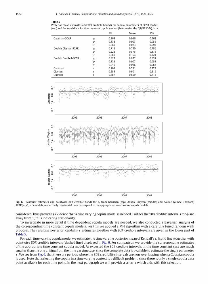
Fig. 6. Posterior estimates and pointwise 80% credible bands for τt from Gaussian (top), double Clayton (middle) and double Gumbel (bottom)SCAR(µ, φ, σ 2) models, respectively. Horizontal lines correspond to the appropriate time constant copula models.

considered, thus providing evidence that a time varying copula model is needed. Further the 90% credible intervals for φ areaway from 1, thus indicating stationarity.

To investigate in more detail if time dependent copula models are needed, we also conducted a Bayesian analysis ofthe corresponding time constant copula models. For this we applied a MH algorithm with a carefully tuned random walkproposal. The resulting posterior Kendall’s τ estimates together with 90% credible intervals are given in the lower part ofTable 5.

For each time varying copulamodel we estimate the time varying posteriormean of Kendall’s τt (solid line) togetherwithpointwise 80% credible intervals (dashed line) displayed in Fig. 6. For comparison we provide the corresponding estimatesof the appropriate time constant copula model. As expected the 80% credible intervals in the time constant case are muchsmaller than the one arising from the time varying case, since the complete data is available to estimate the single parameterτ . We see from Fig. 6, that there are periods where the 80% credibility intervals are non-overlappingwhen a Gaussian copulais used. Note that selecting the copula in a time varying context is a difficult problem, since there is only a single copula datapoint available for each time point. In the next paragraph we will provide a criteria which aids with this selection.

C. Almeida, C. Czado / Computational Statistics and Data Analysis 56 (2012) 1511–1527 1523

Forecasting.To explore the forecasting performance of different SCAR(µ, φ, σ 2)modelswe consider a normalized sum and difference

of the standardized residuals given by

st =12(r1,t + r2,t) and dt =

12(r1,t − r2,t), (23)

where ri,t :=νi−2νi

T−1νi(ui,t), for i = 1, 2 and t = 1, . . . , T . These quantities were chosen since they correspond to scaled ver-

sions of two portfolios, one investing equally in both indices (corresponding to st ) and onewith short selling (correspondingto dt ) often used in pairs trading. We could also investigate the performance of these two portfolios on the original scale ofthe data however, as only the copulas of each model are different, this diagnostic is also appropriate.

The distribution of st and dt depends on the joint distribution of ut , and thus on Cθt , respectively. Therefore st and dtare useful quantities for evaluating the forecasting abilities of a SCAR(µ, φ, σ 2) model. In particular we are interested incomparing one day ahead forecasts for st and dt , respectively. Before doing so, it is instructive to examine the properties ofthese quantities in more detail. By the linearity of the expectation it follows that

E(st | u1:t−1) = E(dt | u1:t−1) = 0 ∀t = 2, . . . , T .

Since V (r1,t | u1:t−1) = V (r2,t | u1:t−1) = 1 holds, we have for t = 2, . . . , T

Cov(st , dt | u1:t−1) =14Cov(r1,t + r2,t , r1,t − r2,t | u1:t−1)

=14

V (r1,t | u1:t−1)− V (r2,t | u1:t−1)

+

14

Cov(r1,t , r2,t | u1:t−1)− Cov(r2,t , r1,t | u1:t−1)

= 0.

Further, we determine

V (st | u1:t−1) =V (r1,t | u1:t−1)+ V (r2,t | u1:t−1)+ 2Cov(r1,t , r2,t | u1:t−1)

4

=1+ E((r1,t r2,t | u1:t−1))

2=

1+ E((E(r1,t r2,t | γt , u1:t−1) | u1:t−1))

2

=12(1+ E(g(γt) | u1:t−1)), (24)

where g(γt) := E(r1,t r2,t | γt , u1:t−1) = E(r1,t r2,t | γt) =(ν1−2)(ν2−2)

ν1ν2

[0,1]2 T

−1ν1

(u)T−1ν2(v)cθt (u, v)d(u, v), and θt defined as

in (4). Similarly it follows that

V (dt | u1:t−1) =12(1− E(g(γt) | u1:t−1)). (25)

Comparing (24) and (25), we see that if µ ≥ 0, the temporal variability of γt has less influence on the conditional varianceof st compared to the one for dt . Further the quantity st is very sensitive to outliers. Thus we expect dt to have higherdiscriminative power than st for different SCAR(µ, φ, σ 2) models.

We now show how theMCMC iterations of the CG sampler can be used to construct one day ahead forecasts for st and dt ,respectively, based on 1000 previous observations (i.e. uℓ−1000:ℓ−1) from 05/14/2008 until 10/31/2008. For this we performthe following steps, for each ℓ = T + 1, . . . , T + 120:

• Run the CG sampler based on uℓ−1000:ℓ−1 for R iterations withMCMC valuesµ(r)ℓ−1, φ

(r)ℓ−1, σ

(r)ℓ−1 and γ

(r)1:ℓ−1 for r = 1, . . . , R.

• Forecast the corresponding latent value γ(r)ℓ by simulating γ

(r)ℓ from N(µ

(r)ℓ−1 + φ

(r)ℓ−1(γ

(r)ℓ−1 − µ

(r)ℓ−1), (σ

(r)ℓ−1)

2).

• Forecast the corresponding copula parameter θ(r)ℓ by setting θ

(r)ℓ := τ−1

exp(2γ (r)

ℓ)−1

exp(2γ (r)ℓ

)+1

.

• Forecast the corresponding copula data (u(r)1,ℓ, u

(r)2,ℓ) by simulating them from C

θ(r)ℓ

and compute the corresponding

forecasts s(r)ℓ and d(r)ℓ using (23).

The continuous rank probability score (CRPS) of Gneiting and Raftery (2007) is a summarymeasure to evaluate forecasts.It takes both forecast precision as well as forecast variability into account. For an illustration of this property see Figure 1 ofGschlößl and Czado (2007). It is defined as follows: Suppose a random quantity X is to be forecasted based on a distributionfunction F(x). If X = x0 is observed the CRPS of x0 is defined as

CRPS(x0) =∞

−∞

|F(x)− 1(−∞,x](x0)|dx.

1524 C. Almeida, C. Czado / Computational Statistics and Data Analysis 56 (2012) 1511–1527

Table 6Average estimated CRPS scores for sℓ and dℓ , respectively.

Type Model CRPS(s(o)) CRPS(d(o))

Time Gaussian-SCAR 0.650 0.126Varying Double Clayton-SCAR 0.651 0.131

Double Gumbel-SCAR 0.648 0.127Time Gaussian 0.656 0.137Constant Clayton 0.664 0.141

Gumbel 0.658 0.137

Table 7Number out of 120 forecast days, where CRPS(s(o)ℓ ) and CRPS(d(o)

ℓ ) are lowerfor the SCAR model compared to the time constant model, respectively.

ns nd

Gaussian-SCAR 48 68Double Clayton-SCAR 68 81Double Gumbel-SCAR 55 71

A forecast distribution with a smaller CRPS is to be preferred. Here the corresponding observed values are defined throwr (o)i,ℓ =

νi−2νi

εi,ℓσi,ℓ

by

s(o)ℓ :=12(r (o)

2,ℓ + r (o)2,ℓ) and d(o)

ℓ :=12(r (o)

2,ℓ − r (o)2,ℓ).

In our situation we want to forecast sℓ based on the Bayesian predictive distribution Fℓ(s) = P(sℓ ≤ s | uℓ−1000:ℓ−1). Asin Panagiotelis and Smith (2008) the corresponding CRPS(s(o)ℓ ) can be estimated by

CRPS(s(o)ℓ ) =1R

Rr=1

|s(r)ℓ − s(o)ℓ | −121R

Rr=1

|s(r)ℓ − s′(r)ℓ |,

where s′(r)ℓ is independently resampled from s(r)ℓ ; r = 1, . . . , R. Similarly a CRPS for dℓ can be defined and estimated by

CRPS(d(o)ℓ ). For all forecast dayswe determine CRPS(s(o)) = 1

120

T+120ℓ=T+1

CRPS(s(o)ℓ ).We define CRPS(d(o)) in a similar fashion.These average estimates are contained in Table 6. It shows that normalized residual sum sℓ is forecasted equallywell by SCARand time constant models regardless of the copula family chosen, while for the normalized residual difference dℓ, the timevarying models are preferred.

We are denoting by ns (nd) the number out of 120 forecast days the statistic CRPS(s(o)ℓ ) ( CRPS(d(o)ℓ )) is smaller for the

time varying SCAR model compared to the corresponding time constant model. These quantities are given in Table 7. Wesee again that different time varying SCARmodels cannot be distinguished from their time constant counterpart with regardto forecasting the normalized residual sum sℓ, but there is a noticeable difference in the quality of forecasts of dℓ. The copulachoice has a higher influence on the forecasting performance of dt than st , thus we expect portfolios with short selling to bemore affected by the choice of the copula type.

In summary we have shown that there is evidence of time varying copula dependence in the residuals for this data set.

6. Summary and outlook

We considered SCAR copula models allowing for stochastic time-varying dependence driven by time dependent latentvariables. The latent variables follow a stationary AR(1) model and the inverse Fisher transform relates the latent variable attime t to the Kendall’s τ at time t . Any one-parameter bivariate copula can be used. For the simulation and applicationwe chose the Gaussian, double Clayton and double Gumbel copula, allowing for positive and negative dependencessimultaneously. The SCAR model formulation allows for easy comparison of different copula families, since the timedependence is modeled in terms of Kendall’s τt and not with respect to the parameter θt which specifies the copulafamily.

We took a Bayesian approach using MCMC sampling for estimation and inference, since maximum likelihood requiresoptimization over computationally intensive T -dimensional integrals with respect to the latent variables. In additionthe Bayesian approach allows easy construction of credible intervals, enabling the assessment of the precision of pointestimates. Further, using the MCMC iterates we can easily construct point-wise credible intervals for interesting time-varying quantities such as Kendall’s τt or the tail dependence coefficient λt , as long there are simple relationships betweenthe copula parameter θt , Kendall’s τt and the tail dependence coefficient λt .

C. Almeida, C. Czado / Computational Statistics and Data Analysis 56 (2012) 1511–1527 1525

The need of having to update all latent variables requires special carewhen aMCMC algorithm is designed.We developedtwo sampling schemes. One is a naïve sampling scheme for the latent variables which uses individual Metropolis–Hastingsteps. This sampler however exhibits large autocorrelations. We improved this sampling scheme by developing a coarsegrid sampler. We found a random transformation satisfying the conditions of Liu and Sabatti (2000), which does not changethe posterior and is easy to sample. In a simulation study we showed that this procedure improves the mixing of the MCMCchain as measured by the effective sample size.

In the application to financial stock indices we demonstrated the need to incorporate time varying dependence. Weapplied the coarse grid sampler for SCAR models with Gaussian, double Clayton and double Gumbel copulas.

There are several interesting open problems to investigate. First, one can develop a joint Bayesian analysis of marginalmodels such as GARCH or stochastic volatility (SV) models as suggested in Ausin and Lopes (2010) using a nonstochasticdependence dynamics.

Second,we can extend this bivariatemodel tomore dimensions by usingmultivariate copulas. A very flexible class of suchmodels has been suggested and applied to financial time series data by Aas et al. (2009). It uses the pair-copula construction(PCC) method and a recent survey of these PCCmodels are given in Czado (2010). The advantage of such an approach is thatthemodel is formulatedwith respect to conditional parameters,which in contrast to correlation parameters in amultivariateGaussian or t-copula can be chosen independently. Time varying dependence can be incorporated in a similar fashion as forthe SCAR copula models. Efficient Bayesian inference for such models is currently being studied.

Finally more suitable model comparison criteria for non-nested SCAR models are needed. One possible approach herewould be to investigate Bayesian adaptations to non-nestedmodel comparison tests such as suggested by Vuong (1989) andClarke (2007). A first such adaptation was provided in Czado et al. (in press) in the context of spatial count data.

Acknowledgments

Claudia Czado and Carlos Almeida gratefully acknowledge the financial support from the Deutsche Forschungsgemein-schaft (Cz 86/1-3: Statistical inference for high dimensional dependence models using pair-copulas). The numerical com-putations were performed on a Linux cluster supported by DFG grant INST 95/919-1 FUGG. We thank the referees for theirhelpful comments and suggestions, which improved the manuscript considerably.

Appendix A. Algorithms

Algorithm 1 Updating latent variables (naïve method).

Input: γ(r−1)t , 1 ≤ t ≤ T

Output: γ(r)t , 1 ≤ t ≤ T

1: for t ← 1, T do2: Simulate γt from N(γ ∗t , σ ∗t

2) ◃ See Eq. (11)

3: Compute k = min

p(ut |γt )p(ut |γ

(r−1)t )

, 1

4: MH-Step:5: if unif(0,1)≤ k, γ (r)

t ← γt

6: else γ(r)t ← γ

(r−1)t

7: end for

Algorithm 2 Updating latent variables (coarse grid method).

Input: γ(r−1)t , 1 ≤ t ≤ T

Output: γ(r)t , 1 ≤ t ≤ T

1: for t ← 1, T do2: Simulate λt from N(λ∗t , Vt)

∗◃ See Eq. (17)

3: Set γ1:T = γ(r−1)1:T + λt bt

4: Compute k = min

p(u1:T |γ1:T )

p(u1:T |γ(r−1)1:T )

, 1

5: MH-Step:6: if unif(0,1)≤ k, γ (r)

1:T ← γ1:T

7: else γ(r)1T← γ

(r−1)1:T

8: end for

1526 C. Almeida, C. Czado / Computational Statistics and Data Analysis 56 (2012) 1511–1527

Algorithm 3 Updating parameters.Input: µ(r−1), φ(r−1), σ (r−1)

Output: µ(r), φ(r), σ (r)

1: Update of µ:2: σ 2(r) from IG(a, b) ◃ see Eq. (20)3: Update of µ:4: µ(r) from N(c, d2) ◃ see Eq. (21)5: Update of φ6: Simulate φ from N

S1S0

, 1S0

· 1[−1,1](φ) ◃ See Eq. (22)

7: Compute k = min1, (1+φ)

e− 12 (1−φ)

f− 12

(1+φ(r−1))e− 1

2 (1−φ(r−1))f− 1

2

,

8: if unif(0,1)≤ k, φ(r)← φ

9: else φ(r)← φ(r−1)

Appendix B. Conditional expectations and variances for the coarse grid method

The values of λ∗t and V ∗t for the definition of bt as in Eq. (13).

For t = 1, 2 : λ∗t = −(γt − µ)+ φ2(γt+2 − µ)

V ∗t = σ 2(1+ φ2)

For t = 3, . . . , T − 2 : λ∗t = −(γt − µ)+φ2(γt−2 + γt+2 − 2µ)

1+ φ4

V ∗t =σ 2(1+ φ2)

1+ φ4

For t = T − 1, T : λ∗t = −(γt − µ)+ φ2(γt−2 − µ)

V ∗t = σ 2(1+ φ2).

References

Aas, K., Czado, C., Frigessi, A., Bakken, H., 2009. Pair-copula constructions of multiple dependence. Insurance: Mathematics and Economics 44 (2), 182–198.Ausin, M.C., Lopes, H.F., 2010. Time-varying joint distribution through copulas. Computational Statistics & Data Analysis 54, 2383–2399.Bauwens, L., Laurent, S., Rombouts, J.V.K., 2006. Multivariate GARCH models: a survey. Journal of Applied Econometrics 21 (1), 79–109.Bollerslev, T., 1986. Generalized autoregressive conditional heteroskedasticity. Journal of Econometrics 31 (3), 307–327.Cherubini, U., Luciano, E., Vecchiato, W., 2004. Copula Methods in Finance. In: Wiley Finance Series, John Wiley & Sons Ltd., Chichester.Chib, S., Greenberg, E., 1994. Bayes inference in regression models with ARMA (p, q) errors. Journal of Econometrics 64 (1–2), 183–206.Clarke, K., 2007. A simple distribution-free test for nonnested hypotheses. Political Analysis 15 (3).Czado, C., 2010. Pair-copula constructions of multivariate copulas. In: Durante, F., Härdle, W., Jaworki, P., Rychlik, T. (Eds.), Workshop on Copula Theory

and its Applications. Springer, Dortrech.Czado, C., Gärtner, F., Min, A., 2011. Analysis of Australian electricity loads using joint Bayesian inference of d-vines with autoregressive margins.

In: Kurowicka, D., Joe, H. (Eds.), Dependence Modeling—Handbook on Vine Copulae. World Scientific Publishing Co.Czado, C., Schabenberger, H., Erhardt, V., 2009. Nonnested model selection for spatial count regression models with application to health insurance.

Statistical Papers (in press).Dias, A., Embrechts, P., 2004. Change-point analysis for dependence structures in finance and insurance. In: Szegoe, G. (Ed.), Risk Measures for the 21th

Century. In: Wiley Finance Series, pp. 32–335.Engle, R., 2002. Dynamic conditional correlation: a simple class of multivariate generalized autoregressive conditional heteroskedasticity models. Journal

of Business & Economic Statistics 20 (3), 339–350.Erb, C.B., Harvey, C.R., Viskanta, T.E., 1994. Forecasting international equity correlations. Financial Analysts Journal 50 (6), 32–45.Frees, E.W., Valdez, E.A., 1998. Understanding relationships using copulas. North American Actuarial Journal 2 (1), 1–25.Genest, C., Ghoudi, K., Rivest, L.-P., 1995. A semiparametric estimation procedure of dependence parameters in multivariate families of distributions.

Biometrika 82 (3), 543–552.Geweke, J., Tanizaki, H., 2001. Bayesian estimation of state-space models using the metropolis-hastings algorithm within gibbs sampling. Computational

Statistics & Data Analysis 37 (2), 151–170.Giacomini, E., Härdle, W., Spokoiny, V., 2009. Inhomogeneous dependence modeling with time-varying copulae. Journal of Business & Economic Statistics

27 (2), 224–234.Gneiting, T., Raftery, A.E., 2007. Strictly proper scoring rules, prediction, and estimation. Journal of the American Statistical Association 102 (477), 359–378.Gschlößl, S., Czado, C., 2007. Spatial modelling of claim frequency and claim size in non-life insurance. Scandinavian Actuarial Journal 107, 202–225.Hafner, C.M., Manner, H., 2010. Dynamic stochastic copula models: estimation, inference and applications. Journal of Applied Econometrics.Harvey, A., Ruiz, E., Shephard, N., 1994. Multivariate stochastic variance models. The Review of Economic Studies 61 (2), 247–264.Hastings, W.K., 1970. Monte Carlo sampling methods using Markov chains and their applications. Biometrika 57 (1), 97–109.Hofmann, M., Czado, C., 2010. Assessing value-at-risk using joint Bayesian inference of d-vines with GARCH (1,1) margins (submitted for publication).Joe, H., 1996. Families of m-variate distributions with given margins and m(m − 1)/2 bivariate dependence parameters. In: Distributions with Fixed

Marginals and Related Topics. Seattle, WA, 1993. In: IMS Lecture Notes Monogr. Ser., Vol. 28. Inst. Math. Statist., Hayward, CA, pp. 120–141.Joe, H., 1997. Multivariate Models and Dependence Concepts. In: Monographs on Statistics and Applied Probability, vol. 73. Chapman & Hall, London.Joe, H., 2005. Asymptotic efficiency of the two-stage estimation method for copula-based models. Journal of Multivariate Analysis 94 (2), 401–419.Jondeau, E., Rockinger, M., 2006. The copula-GARCHmodel of conditional dependencies: an international stockmarket application. Journal of International

Money and Finance 25, 827–853.

C. Almeida, C. Czado / Computational Statistics and Data Analysis 56 (2012) 1511–1527 1527

Kim, G., Silvapulle, M.J., Silvapulle, P., 2007. Comparison of semiparametric and parametric methods for estimating copulas. Computational Statistics &Data Analysis 51 (6), 2836–2850.

Liesenfeld, R., Richard, J.-F., 2003. Estimation of dynamic bivariate mixture models: comments on Watanabe (2000). Journal of Business & EconomicStatistics 21 (4), 570–576.

Liu, Y., Luger, R., 2009. Efficient estimation of copula-GARCHmodels. Computational Statistics & Data Analysis 53 (6), 2284–2297. (The Fourth Special Issueon Computational Econometrics).

Liu, J.S., Sabatti, C., 2000. Generalised Gibbs sampler and multigrid Monte Carlo for Bayesian computation. Biometrika 87 (2), 353–369.Longin, F., Solnik, B., 1995. Is the correlation in international equity returns constant: 1960–1990? Journal of International Money and Finance 14 (1), 3–26.Manner, H., Candelon, B., 2007. Testing for asset market linkages: a new approach based on time-varying copulas. METEOR Research Memorandum (RM)

07/052.Manner, H., Reznikova, O., 2009. Time-varying copulas: a survey. Institut de Statistique UCL, DP0917.Mercurio, D., Spokoiny, V., 2004. Statistical inference for time-inhomogeneous volatility models. Annals of Statistics 32 (2), 577–602.Nelsen, R.B., 2006. An Introduction to Copulas, 2nd ed. In: Springer Series in Statistics, Springer, New York.Panagiotelis, A., Smith, M., 2008. Bayesian density forecasting of intraday electricity prices using multivariate skew t distributions. International Journal of

Forecasting 24 (4), 710–727.Patton, A.J., 2006. Estimation of multivariate models for time series of possibly different lengths. Journal of Applied Econometrics 21 (2), 147–173.Richard, J.-F., Zhang, W., 2007. Efficient high-dimensional importance sampling. Journal of Econometrics 141 (2), 1385–1411.Sklar, M., 1959. Fonctions de répartition à n dimensions et leurs marges. Publications de l’Intitut de Statistique de l’Universit de Paris 8, 229–231.Tanner, M.A., Wong, W.H., 1987. The calculation of posterior distributions by data augmentation. Journal of the American Statistical Association 82 (398),

528–540.Taylor, S.J., 1986. Modelling Financial Time Series. John Wiley and Sons.Tse, Y.K., Tsui, A.K.C., 2002. A multivariate generalized autoregressive conditional heteroscedasticity model with time-varying correlations. Journal of

Business & Economic Statistics 20 (3), 351–362.Vuong, Q.H., 1989. Likelihood ratio tests for model selection and nonnested hypotheses. Econometrica 57 (2), 307–333.Yu, J., Meyer, R., 2006. Multivariate stochastic volatility models: Bayesian estimation and model comparison. Econometric Reviews 25, 361–384.