ARTICLE

Efficiency stagnation in global steel productionurges joint supply- and demand-side mitigationeffortsPeng Wang1,2, Morten Ryberg 3✉, Yi Yang1,4,5, Kuishuang Feng 6,7, Sami Kara 2✉, Michael Hauschild3 &

Wei-Qiang Chen 1,8✉

Steel production is a difficult-to-mitigate sector that challenges climate mitigation commit-

ments. Efforts for future decarbonization can benefit from understanding its progress to date.

Here we report on greenhouse gas emissions from global steel production over the past

century (1900-2015) by combining material flow analysis and life cycle assessment. We find

that ~45 Gt steel was produced in this period leading to emissions of ~147 Gt CO2-eq.

Significant improvement in process efficiency (~67%) was achieved, but was offset by a

44-fold increase in annual steel production, resulting in a 17-fold net increase in annual

emissions. Despite some regional technical improvements, the industry’s decarbonization

progress at the global scale has largely stagnated since 1995 mainly due to expanded pro-

duction in emerging countries with high carbon intensity. Our analysis of future scenarios

indicates that the expected demand expansion in these countries may jeopardize steel

industry’s prospects for following 1.5 °C emission reduction pathways. To achieve the

Paris climate goals, there is an urgent need for rapid implementation of joint supply- and

demand-side mitigation measures around the world in consideration of regional conditions.

https://doi.org/10.1038/s41467-021-22245-6 OPEN

1 Key Lab of Urban Environment and Health, Institute of Urban Environment, Chinese Academy of Sciences, Xiamen, China. 2 Sustainability in Manufacturingand Life Cycle Engineering Research Group, School of Mechanical and Manufacturing Engineering, The University of New South Wales, Sydney, Australia.3 Quantitative Sustainability Assessment Group, Sustainability Division, Department of Technology, Management and Economics, Technical University ofDenmark, Kgs, Lyngby, Denmark. 4 Key Laboratory of the Three Gorges Reservoir Region’s Eco-Environment, Ministry of Education, Chongqing University,Chongqing, China. 5 Environmental Studies Program, Dartmouth College, Hanover, NH, USA. 6 Institute of Blue and Green Development, ShandongUniversity, Weihai, China. 7 Department of Geographical Sciences, University of Maryland, College Park, MD, USA. 8 University of Chinese Academy ofSciences, Beijing, China. ✉email: moryb@dtu.dk; s.kara@unsw.edu.au; wqchen@iue.ac.cn

NATURE COMMUNICATIONS | (2021) 12:2066 | https://doi.org/10.1038/s41467-021-22245-6 | www.nature.com/naturecommunications 1

1234

5678

90():,;

Steel is the most used metal in our modern world, but itsproduction is highly energy- and carbon- intensive. Toachieve a climate-safe future as required by the Paris

Agreement, there is a need for reaching net-zero emissions byaround 2050 and net negative emissions thereafter1,2 for everysector including the steel industry3,4. However, steel production,together with other energy-intensive industries such as cementand petrochemicals, is considered a difficult-to-mitigate sector5–7.Their decarbonisation remains extremely challenging on thefollowing grounds: First, their global demands are projected toincrease to support a growing and increasingly affluentpopulation8,9. Second, some carbon-based resource is essential forhigh-temperature heat and steelmaking and cannot be easilyreplaced7,10,11. Third, the long-lived facilities in their productionmay further hinder the required mitigation progress due to thecarbon lock-in effect12,13. Thus, compared to transportation andenergy sectors, the corresponding innovation, progress andunderstanding related to the decarbonisation of global steelindustry are generally lagging behind14–16.

Strategies for decarbonising the steel industry have primarilyfocused on production efficiency improvement, including energyefficiency measures10,17,18, production technologies innovation19,20

and fuel switching21–23. However, the effectiveness of suchproduction-based strategies in terms of carbon reduction hasrecently been questioned3,14,24,25. This calls for attention to gaugethe entire progress that the global steel industry has made on GHGmitigation. Most of previous investigations have been limitedto specific production technologies24,26,27 where the interplaybetween material flows and supply-side technical efficiency waswidely overlooked. Such lack of understanding could prohibit thedevelopment of strategies that are more effective for steel industrytoward future GHG emission mitigation.

Here, we integrated dynamic material flow analysis (MFA)with life cycle assessment (LCA) to estimate annual production,efficiency and GHG emissions of global steel production based on19 dominant processes during 1900–2015. By examining theinterplay between material flows and GHG emissions, we foundan exponential increase in steel production volume (ca. 3.4%/year) and associated GHG emissions (ca. 2.5%/year) over the past115 years, despite a concomitant reduction in the carbon emis-sions intensity by ~67% achieved through technical innovationand efficiency improvement. We then performed a decomposi-tion analysis to reveal the contribution of efficiency improvementand production outputs to these emission changes, the results ofwhich highlighted the inadequacy of process efficiency alone inachieving absolute emissions reduction. We found that the GHGintensity of the global steel industry had stagnated in the past15–20 years before 2015. By region specific investigation, wefound that there were improvements in technology efficienciesduring the past few decades but these were offset by the con-comitant growth of steel production with low process efficiency(especially in China and India). This stagnation indicates theurgency of the joint implementation of process efficiency anddemand-side measures to reduce GHG emissions and achieveclimate targets.

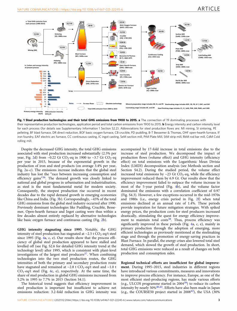
Results and discussionGHG emissions weigh three times more than the steel pro-duced. We estimate that global steel production emitted a total of~147 billion tonnes (Gt) CO2-eq from 1900 to 2015, accountingfor ~9% of global GHG emissions during this period (see Fig. 1 foreach process, with additional details in Section S1.2). The iron-making stage contributed the most (around 50%) to the totalemissions, caused mainly by the use of carbon as a fuel and as areductant in the blast furnace (i.e., 58 Gt)27. The steelmaking stage

(excluding iron foundry) emitted 33 Gt of CO2-eq totally, of whicharound half pertained to the open-hearth furnace (Fig. 1a).Despite a much lower carbon intensity (Fig. 1b), the steel finishingstage emitted 27 Gt CO2-eq mainly due to the vast productionflows (Fig. 2c). Over the studied period, the total GHG emissionsfrom mineral treatment were 18.7 Gt CO2-eq and this number isexpected to increase in the future as a result of decreasing oregrade. The entire production system can be divided into twomajor production routes (see Fig. S1.2), i.e., the primary route withthe ore-blast furnace system and the secondary route with scrap-electric arc furnace system. They differ substantially in terms ofefficiency, resource use, emissions, and production volumes28–30.The secondary production route was around one-eighth ascarbon-intensive as the primary route31, and accounted for ~5% oftotal annual GHG emissions in 2015 as shown in Fig. 2d, e.Historically, it is estimated that the primary production routeemitted 132 Gt CO2-eq over the studied period, accounting forover 90% of the total GHG emissions from steel production.

Figure 3a presents the cumulative flows and stocks of steel alongits material cycle from 1900 to 2015. Our analysis shows that thesteel industry consumed ~46 Gt iron ore and ~31 Gt home, newand old scrap to produce ~45 Gt steel products during this period,which, in terms of weight, is around one-third of the total steelproduction-related GHG emissions (147 Gt CO2-eq). At present,over half of those steel products remain as societal in-use stocks(i.e., ~25 Gt) with the largest share stored in buildings (~16 Gt)which were mainly constructed in the past 20 years (driven by largeemerging economies, including China and India32). In general,those societal in-use stocks are quite young with ~83% of globalsteel in-use stocks being built after 1990 (Fig. 3a). Given that theaverage lifetime of steel products is ~70 years9, a rapid increase inold scrap generation can be foreseen in these countries over the next30–50 years. Indeed, the past few decades have already witnessed asignificant increase in old scrap generation from ~45 Mt/year in1950 to ~427 Mt/year in 2015 (Fig. 2g), concomitant with aremarkable improvement in steel recycling rate (now remaining ataround 70%) (Fig. 2h). However, such an increase may not lead to anet decrease in steel production-related GHG emissions, as this willdepend on the future increase in total steel demand and whether itcan be, to a large extent, satisfied by secondary steel production33.Unfortunately, our analysis shows that these improvements havenot kept up with the fast growth in steel consumption in recentdecades as in-use stocks in emerging economies like China were tooyoung (average age: 8.6 years in Fig. 3a) to generate enough oldscrap, forcing regional steel production to rely heavily on ironores34. This led to a notable decrease in the share of secondaryproduction relative to primary production from 30% in 1995 to21% in 2015 (Fig. 2i), contributing partly to the increase of thesector’s total GHG emissions.

Efficiency improvement offset by demand growth. Given thatenergy constitutes 20–40% of total steel production costs35, steelproducers have a strong incentive to improve their energy effi-ciency. Our analysis shows that the steel industry has reducedGHG emissions intensity by ~67% since 1900 (Fig. 4a), and thesteepest decrease occurred before 1940 due to energy efficiencyimprovement in the blast furnace27. After the 1940s, the largestdrop in emissions intensity occurred between 1970 and 1995(from ~4.5 to 2.6 t CO2-eq/t steel), due to the improvement inenergy efficiency through technological advances, such as the useof pelletizing in lieu of sintering for ore preparation and increaseduse of BOF instead of open-hearth furnace. Moreover, the con-tinued decarbonisation of the electricity grid since the energycrisis in the 1970s has also contributed substantially to loweringthe GHG intensity of steel production (Table S2.5–S2.6).

ARTICLE NATURE COMMUNICATIONS | https://doi.org/10.1038/s41467-021-22245-6

2 NATURE COMMUNICATIONS | (2021) 12:2066 | https://doi.org/10.1038/s41467-021-22245-6 | www.nature.com/naturecommunications

Despite the decreased GHG intensity, the total GHG emissionsassociated with steel production increased substantially (2.5% peryear, Fig. 2d) from ~0.22 Gt CO2-eq in 1900 to ~3.7 Gt CO2-eqper year in 2015, because of the exponential growth in theproduction of iron and steel products (on average 3.4% per year,Fig. 2a–c). The emissions increase indicates that the global steelindustry has lost the “race between increasing consumption andefficiency gains”36. The demand growth was closely linked tonational and global progress in urbanisation and industrialisation,as steel is the most fundamental metal for modern society.Consequently, the steepest production rise occurred in recentdecades due to the rapid demand growth in emerging economieslike China and India. (Fig. 3b). Correspondingly, ~45% of the totalGHG emissions from the global steel industry occurred after 1990.Previously dominant technologies like Puddling, Crucible, Besse-mer, Open-hearth furnace and Ingot casting were thus within afew decades almost entirely replaced by alternative technologieslike basic oxygen furnace and continuous casting (Fig. 2b).

GHG intensity stagnating since 1995. Notably, the GHGintensity of steel production has stagnated at ~2.5 t CO2-eq/t steelsince 1995 (Fig. 4a, c, e). Our results show that the process effi-ciency of global steel production appeared to have stalled andlevelled off (see Fig. S2.6 for detailed GHG intensity trend at thetechnology level) after 1995, which is consistent with plant-levelinvestigations of the largest steel producers37. When combiningtechnologies into the two steel production routes, the GHGintensities of both the primary and secondary production routehave stagnated and remained at ~2.8 t CO2-eq/t steel and ~1.0 tCO2-eq/t steel (Fig. 4c, e), respectively. At the same time, theshare of steel production in global GHG emissions increased from5.2% in 1995 to 7.7% in 2015 (Section S4.1).

The historical trend suggests that efficiency improvement insteel production is important but insufficient to achieve netemissions reduction: 3.2-fold reduction in GHG intensity was

accompanied by 17-fold increase in total emissions due to theincrease of steel production. We decomposed the impact ofproduction flows (volume effect) and GHG intensity (efficiencyeffect) on total emissions with the Logarithmic Mean DivisiaIndex (LMDI) decomposition analysis (see Methods section andSection S4.2). During the studied period, the volume effectincreased total emissions by ~23 Gt CO2-eq, while the efficiencyimprovement reduced them by 6.9 Gt. Our results show that theefficiency improvement failed to outpace the volume increase inmost of the 5-year period (Fig. 4b), and the volume factordominated the emissions with a correlation coefficient of 0.97(Fig. S4.3). However, a few exceptions occurred in the mid-1970sand 1980s (i.e., energy crisis period in Fig. 2f) when totalemissions declined at an annual rate of 1.4%. These periodsprovide inspiration for future mitigation strategies. With spikedenergy prices, the production costs for steel producers increaseddrastically, stimulating the quest for energy efficiency improve-ment to maintain total costs38. Thus, process efficiency wassignificantly improved in these periods (Fig. 4a, c, e), mainly inprimary production through the adoption of emerging, moreefficient technologies as previously mentioned at the steelmakingstage and through the promotion of energy-saving practices inBlast Furnace. In parallel, the energy crises also lowered total steeldemand, which slowed the growth of steel production. In short,total GHG emissions were reduced as a result of changes on bothproduction and consumption sides.

Regional technical efforts are insufficient for global improve-ment. During 1995–2015, steel industries in different regionshave introduced various commitments, measures and innovationsto improve process efficiency. For instance, Europe, as one of themost efficient steel-producing regions, has made various efforts(e.g., ULCOS programme started in 200439) to reduce its carbonintensity by nearly 50%40,41. Efforts have also been made in Japan(e.g., the COURSE50 project started in 200842), the USA (30%

5.5 Gt

Mining (MI)

12.7 Gt

Sintering(SI): 1880s-now

0.5 Gt

Pelle�ng(PE): 1880s-now

GHG emission intensity(tCO2/t)

Primary energy intensity (GJ/t)

0 5 10 15 20

MISI

PEDRBF

OHFBOFEAF

CCICIF

SeMRbMPtMStM

CdM

0123

Blast Furnace(BF): 1400s-now

58 Gt

Direct Reduc�on(DR): 1970s-now

1.2 Gt

Scrap

Electric Arc Furnace(EAF): 1878-now

Basic Oxygen Furnace(BOF): 1952-now

Open Hearth Furnace(OHF): 1864-now

Crucible(CB): 1740-1921

Iron Foundry(IF): 1700s-now

Pudding(PD): 1785-1925

Bessemer & Thomas(B-T): 1860-1975

9.9 Gt

0.2 Gt

0.06 Gt

0.8 Gt

15 Gt

6.8 Gt

7.0 Gt

Con�nuous Cas�ng(CC): 1955-now

Ingot Cas�ng(IC): 1900s-now

0.6 Gt

3.0 Gt

0.7 Gt

Sec�on Mill(SeM): 1500s-now

Plate Mill(PtM): 1800s-now

Strip Mill(StM): 1800s-now

Rod & Bar Mill(RbM): 1800s-now

Cold Rolling Mill(CdM): 1926-now

1.2 Gt

4.3 Gt

5.0 Gt

7.7 Gt

a. Total GHG emission from each process (1900-2015)

b. Carbon and energy intensity of present process

Note:

Total GHG emission from 1900 to 2015

Fe mass flows Mineral prepara�on stage includes MI, SI, and PE

Ironmaking stage includes BF, and DR

Steelmaking stage includes BOF, CB, PD, B-T, OHF, and EAF

Steel finishing stage includes CC, IC, SeM, PtM, StM, RbM, and CdM

Obsolete technology

Fig. 1 Steel production technologies and their total GHG emissions from 1900 to 2015. a The connection of 19 dominating processes withtheir representative production technologies, application period and total carbon emissions from 1900 to 2015. b Energy intensity and carbon intensity levelfor each process (for details see Supplementary Information 1 Section S2.2). Abbreviations for steel production flows are: MI mining, SI sintering, PEpelleting, BF blast furnace, DR direct reduction, BOF basic oxygen furnace, CB crucible, PD puddling, B-T Bessemer & Thomas, OHF open-hearth furnace, IFiron foundry, EAF electric arc furnace, CC continuous casting, IC ingot casting, SeM section mill, PtM Plate Mill, StM strip mill, RbM rod bar mill, CdM Coldrolling mill.

NATURE COMMUNICATIONS | https://doi.org/10.1038/s41467-021-22245-6 ARTICLE

NATURE COMMUNICATIONS | (2021) 12:2066 | https://doi.org/10.1038/s41467-021-22245-6 | www.nature.com/naturecommunications 3

energy intensity reduction since 199043) and other nations. Withthe help of continuous technological advancements and earlyretirement of redundant inefficient facilities, China has also madeprogress in improving its steel production efficiency (by ~30%44)during the past few decades. Moreover, the state-of-the-artironmaking technology blast furnace is approaching the practicalminimum energy requirement31. Nevertheless, those regionaltechnical improvements are found to be insufficient to reduce theoverall GHG intensity (let alone the total GHG emission) of steelproduction at the global level (as indicated in Fig. 3b, c) due to thestructural changes in regional production flows.

By categorising those regions into different groups based ontheir emissions intensities (i.e., Tier 1, 2 and 3 in Fig. 3b), we find

an 8-fold expansion of crude steel production flows from themost carbon-intensive regions (i.e., Tier 3; Fig. 3c), rising from129 Mt/year in 1995 to 914 Mt/year in 2015. By contrast, theoperating production capacity from low (Tier 1) and medium(Tier 2) carbon-intensive regions has shrunk in the same period(Fig. 3b). Indeed, the share of global steel production in Tier 1and 2 regions decreased from 83% to 43% during the studiedperiod. The change in production flow structure has offset thementioned regional technical advances. Notably, the poor carbonperformance of Tier 3 regions was not simply attributed to theirtechnical backwardness45, but also closely linked to the distribu-tion between primary and secondary production routes. Emer-ging economies have been fuelled by the fast expansion of steel

Fig. 2 The steel production technologies and their annual production and GHG emissions from 1900 to 2015. a–c Annual production flows fromeach production technology, derived from dynamic material flow analysis (details see Supplementary Information 1 Section S3.1, Unit: Million tons/year).d–f Annual greenhouse gas (GHG) emissions from primary, secondary and total production routes. The GHG emissions represent the sum of scope 1–3emissions taking a life cycle assessment approach with scope 1 covering the direct emissions from the production site, Scope 2 including the indirectemissions from the energy used for the production and Scope 3 including indirect emissions associated with other inputs used in the steel production.g The historical trend of old scrap generation. h The estimated End-of-life (EoL) steel scrap recycling rate, calculated year by year from our dynamicmaterial flow analysis. i The relative contribution of the secondary production route to total steel production. Data for d–i are presented as the deterministicresults and the shaded areas indicate the 95% confidence interval of the estimates. Abbreviations for steel production flows are: MI mining, SI sintering, PEpelleting, BF blast furnace, DR direct reduction, BOF blast oxygen furnace, CB crucible, PD puddling, BT Bessemer & Thomas, OHF open-hearth furnace, IFiron foundry, EAF electric arc furnace, CC continuous casting, IC ingot casting, SeM section mill, PtM plate mill, StM strip mill, RbM rod bar mill, CdM coldrolling mill.

ARTICLE NATURE COMMUNICATIONS | https://doi.org/10.1038/s41467-021-22245-6

4 NATURE COMMUNICATIONS | (2021) 12:2066 | https://doi.org/10.1038/s41467-021-22245-6 | www.nature.com/naturecommunications

flows (production and consumption) and limited scrap avail-ability. Thus, the production was dominated by the primaryproduction route, which resulted in high GHG intensity for theentire steel industry (see the comparison between the USA andChina46,47). Accordingly, our results highlight the necessity ofcoordinating the implementation of low-carbon technologieswhile also considering the regional structural changes in steelflows (particularly for emerging economies) to achieve deepdecarbonisation of global steel production.

Achievement of 1.5 °C climate target is jeopardized. Future steelflow projections indicate a continuation of the observed historicalpathway: steel demand in emerging economies continuing to growand the ratio of scrap-based production flow remaining at 20–30%till 2035. As a consequence, the global GHG emissions intensity willunlikely to decrease in the near future. The recent World SteelAssociation’s statistics48 has also confirmed that emissions intensityhad been stagnant from 2015 to 2019. In connection to the 1.5 °Cclimate target, this means that 37% of the GHG emissions budget

Mining Preparation Ironmaking Steelmaking Casting Rolling and Finishing Fabrication In-use

SI

BFBOF CC

StM CdMMI

Reserve:53,962

Iron ore:45,942

PE

Sinter: 35,867

Pellet: 5,781

DRI

Pig iron: 36,567

1,101

Home scrap: 11,665

Recycled new and old scrap:

15,000

Internal recycling

EAF

BM

CB

26,042

12,343

12,262

1,080

76

19

2,886IF

PD

OHF IC

27,409

15,863

RbM

PtM

SeM

HR CSS:14,265

HR Bars:17,989

Plates: 4,018

Shapes: 3,013

16,091

Construc�on

Transporta�on

Machinery

Consumer Goods

18,763

5,749

7,069

6,582

End-of-life

New and old scrap generation: 20,700

Period: 1900-2015; Unit: Million tons; S: Stock amount (Unit: Million tons); A: Average age of exis�ng stock (unit: year); P: Stock per capita (cap. in box)

Flows

Processes

EU

NA

DAO

CN

IN

LAC

12,867

287

AF

428

6036

7330

975

4815

1202

4,718

2,537

100

506

132

1,206

150

204

S: 8,089 A: 25P: 11.2 ton/cap.

DAM

S:3,506 A: 27P: 9.82 ton/cap.

S:3,413 A: 18P: 17.8 ton/cap.

S:6,824 A: ~8.6P: 4.7 ton/cap.

S: 844 A: ~11P: 0.64 ton/cap.

S: 324 A: ~17 P: 0.29 ton/cap.

S:825 A: ~16P: 1.32

S:1,052 A: ~12P: 0.7

Stocks

0 1 2 30300600900 0300600900

Exis�ng opera�ng capacity 1995 and 2015 (Mt)

Representa�ve CO2 intensity of steel produc�on in 2016 (tCO2/t steel)

CN

IN

DAM

AF

DAO

LAC

NA

EU

1995 2015 Tier 1 Tier 2 Tier 3

0

400

800

1200

1600

2000

1995 2000 2005 2010 2015

Tier 1

Tier 2

Tier 3

0%

20%

40%

60%

80%

100%

1995 2015

Crude steel produc�on of different CO2 intensity group

EU NA DAM AF DAO LAC IN CN

Tier 1

Tier 2

Tier 3

b. c.

Crud

e st

eel p

rodu

c�on

(Uni

t: M

t/ye

ar)

a.

Shrinking of high efficient produc�on in steel-mature na�ons

Expansion of low efficient produc�on in steel-emerging na�ons

Produc�on ra�o

Fig. 3 Historical steel flows and stocks along with its life cycle, and the recent trend of regional flows since 1995. a The global historical steel cycle in aSankey diagram where the numbers represent the accumulated annual flows over the past 115 years. b The change in operating production capacity foreach studied region between 1995 and 2015, which is assumed to equal annual crude steel production based on data from World Steel Associationyearbook73. The CO2 intensities of these regions are obtained based on the benchmark investigation of Global Efficiency Intelligence45 where only a limitednumber of nations is collected for the comparison of the situation45 in the year 2016. The boundary for this calculation differs from ours, so we onlycategorised these nations into three efficiency tiers (i.e. EU and NA in tier 1, LAC, DAO, AF and DAM in tier 2 and IN and CN in tier 3) for indicativeanalysis. c The annual trend of steel production in the studied regions, which demonstrates that the historical growth in production flow was driven by theemerging nations (China, India, etc.) with poor efficiency performance (described in Section S4.3) as shown in their share change between 1995 and 2015.The abbreviations for regions are: EU Europe, NA North America, DAO Developed Asia and Oceania, AF Africa, DAM Developing Asia and Middle East,LAC Latin America and the Caribbean, IN India, CN China. Abbreviations for steel production flows are: MI mining, SI sintering, PE pelleting, BF blastfurnace, DR direct reduction, BOF blast oxygen furnace, CB crucible, PD puddling, BT Bessemer & Thomas, OHF open-hearth furnace, IF iron foundry, EAFelectric arc furnace, CC continuous casting, IC ingot casting, SeM section mill, PtM plate mill, StM strip mill, RbM rod bar mill, CdM cold rolling mill.

NATURE COMMUNICATIONS | https://doi.org/10.1038/s41467-021-22245-6 ARTICLE

NATURE COMMUNICATIONS | (2021) 12:2066 | https://doi.org/10.1038/s41467-021-22245-6 | www.nature.com/naturecommunications 5

for steel production until 2050 has already been exhausted49. Fur-thermore, if the stagnation trend continues (as assumed in our BAUscenario; S1 in Fig. 5b), the entire carbon budget for steel produc-tion until 2050 could be fully exhausted by around 2035 to meet thegrowing steel demand. Meanwhile, the remaining carbon budgetwill also be exhausted before 2040 despite the implementation ofeither low-carbon technologies (S2 in Fig. 5b) or material efficiency(S3 in Fig. 5b) as indicated in IEA SDS (sustainable developmentscenario) trend31. Accordingly, we revisited previous GHG emissionprojections and found that meeting the 1.5 °C climate target49 isunlikely unless we achieve a radical and immediate intensityreduction with an average rate of 0.85 t CO2-eq/t steel per decade tobecome fully carbon-neutral by 2047 (S4 in Fig. 5b) or an additional34% reduction in steel demand31 (S5 in Fig. 5b). It will require arapid innovation and implementation of low-carbon technologies toachieve the necessary reduction in GHG intensity. We summarised

37 types of breakthrough technologies in Section S4.5 and groupedthem into seven categories: (a) Hydrogen-based options, (b)Electrolysis-based options, (c) CCUS with direct/smelting reduc-tion, (d) Biomass-based options, (e) Blast furnace-improvement, (f)Carbon-free EAF and (g) Low-carbon rolling technologies. Incombination, the breakthrough technologies have the potential toreduce GHG emissions at the required rate to become carbon-neutral by 2047. However, the rate of technology development andimplementation is critical. To realise the 1.5 °C climate target,breakthrough technologies must be developed to a level that is fullyoperational and be implemented at global scale. Based on the reviewof the 37 breakthrough technologies, the rate of developmentappears too slow as most technologies are planned to be available in10–25 years and with only limited implementation at that time.Aside from supply-side technology measures, various demand-sidemitigation measures targeting material flows and technically

-2

-1

0

1

2

3

4

5

0

1

2

3

4

5

1900 1923 1946 1969 1992 2015

0

2

4

6

8

10

1900 1923 1946 1969 1992 2015

0

2

4

6

8

10

1900 1923 1946 1969 1992 2015

a. Steel production-GHG intensity(Unit: t CO2-eq/t steel)

Scope 2

Scope 1

Scope 3

c. Primary production-GHG intensity(Unit: t CO2-eq/t steel)

Scope 2

Scope 1

Scope 3

e. Secondary production-GHG intensity(Unit: t CO2-eq/t steel)

Scope 2

Scope 1

Scope 3

Volumechange rate

Intensitychange rate

Emission change rate

b. Emission Decomposition for steel production(Unit: Gt CO2-eq)

-2

-1

0

1

2

3

4

5d. Emission Decomposition for primary production(Unit: Gt CO2-eq)

-0.2

-0.1

0.0

0.1

0.2

0.3

0.4

0.5 f. Emission Decomposition for secondary production(Unit: Gt CO2-eq)

The 1st-23rd of 5-year period

The 1st-23rd of 5-year period

The 1st-23rd of 5-year period

Fig. 4 Improvement in the steel process efficiency and its linkages with production volume and GHG emission. a, c, e The historical GHG intensityevolution in scopes 1, 2 and 3 for the total, primary and secondary production routes respectively. The red dot line highlights the start of a staggering period(see Supplementary Information 1 Section S4.3). We further decomposed the factors of volume and intensity from total emission impact (seeSupplementary Information 1 Section S4.2). b, d, f The changes in emissions, volume and intensity during the 1st to 23rd 5-year period for total, primary andsecondary production routes, respectively.

ARTICLE NATURE COMMUNICATIONS | https://doi.org/10.1038/s41467-021-22245-6

6 NATURE COMMUNICATIONS | (2021) 12:2066 | https://doi.org/10.1038/s41467-021-22245-6 | www.nature.com/naturecommunications

assisted lifestyle change beyond the direct control of the industryhave received attention25,50,51.

Given the pressing carbon constraints on the steel industry, weargue the need for integration of supply-side and demand-sidemeasures to meet the 1.5 °C climate target. Indeed, a combination ofsupply- and demand-side measures would entail less radicalreduction measures on both sides compared to if either side wouldneed to achieve the reductions alone. We will not venture into thesetup of such a combination and whether the GHG reductionrequirements should be shared equally between the two sides or if acertain split should be applied. However, a combination of effortsbetween supply- and demand side is likely to achieve the 1.5 °C

climate target at a quicker rate as the reduction requirements, to alarger extent, can be based on existing or nearly operational supply-side technology measures and demand-side mitigation measures.Indeed, the actual supply- and demand-side measures must bespecialised based on regional steel flow and technical features. Thecorresponding region-specific priorities are suggested as follows:

(1) Harnessing emerging low-carbon technologies in emergingsteel markets. As our analysis indicates, global steel producershave actively made progress on the innovation and adoptionof emerging technologies31. Again, the effectiveness of low-carbon technologies on climate mitigation lies in their

0

30

60

90

2019 2024 2029 2034 2039 2044 2049

0

50

100

150

200

250

2010 2020 2030 2040 2050

S1

S2

S3

S4

S5

b. Cumula�ve GHG emission from global steel produc�on(Gt CO2e)

IEA-1.5DS:GHG budget (2010-2050)~106 Gt CO2-eq 37% of which has been exhausted by 2019

0.00

0.50

1.00

1.50

2.00

2.50

2000 2010 2020 2030 2040 2050

Stagna�ng efficiency1

IEA-1.5DS

30% lower0.71 tCO2/t in 2050

Less material for same service

(34% demand reduc�on compared to SDS)

a. Future regional steel produc�on flows (Mt/year)

IEA-1.5DS

2

1

3

4

5

1 2 4 3

5

Radical technical efficiency improvement

(0.85 tCO2/t reduc�on per decade)

423

5

c. Cumula�ve steel demand under different scenarios(Gt)

d. Steel emission intensity trend (t CO2e/t steel)

Demand expansion scale 2050/2020

10.50 32Global average level: 1.34

La�n America and Caribbean

5

0

100

200

300

2020 2035 2050

0

100

200

300

2020 2035 20500

100

200

2020 2035 2050

0

200

400

600

800

1000

1200

2020 2035 2050

0

100

200

300

400

500

2020 2035 2050

0

100

200

300

400

500

2020 2035 2050

0

100

200

2020 2035 2050

North AmericaEurope

Developed Asia and Oceania

India

Developing Asia and Middle East

China

Scrap

Scrap

Scrap

Scrap

Scrap

Scrap

Scrap

Scrap genera�on amount in 2050 (Mt/year)

Primary produc�on amount (Mt/year)

Secondary produc�on amount (Mt/year)

0

100

200

300

2020 2035 2050

Africa

Scrap

Fig. 5 Feasibility of material and technical efficiency improvement scenarios to avoid the exhaustion of steel-related 1.5DS carbon budgets. Scenariosare intended to represent explorative estimations rather than actual projections, and their settings are given in Supplementary Information 1 Section S4.4.a The regional growth of steel production flows from primary and secondary production routes (obtained from IEA Stated Policy Scenario (SPS) from itslatest steel report31) and scrap generation (our calculation of scraps is based on the method from Pauliuk et al.9). We also adopt scenario analysis ofrequired efficiency improvement trends under the 1.5DS carbon budget based on the projections of global steel production flows. b, c, d Six potentialscenarios are generated for global steel production flows, i.e., Scenario 1(S1) BAU with ongoing stagnating efficiency trend with IEA SPS demand trend,Scenario 2(S2) with technical efficiency improvement under IEA’s sustainable development scenario with 30% intensity reduction by 2050, and Scenario 3(S3) with material efficiency improvement under IEA’s sustainable development scenario with 12% reduction of total steel demand. All scenarios 1–3 willexhaust the carbon budget before 2050 as shown in Fig. 5b. Thus, Scenario 4(S4) and Scenario 5(S5) test the potential need of radical technical efficiencyimprovement (i.e. 0.85 t CO2-eq/t steel reduction per decade) and material efficiency improvement (i.e. 34% additional demand reduction compared toIEA Sustainable Development Scenario) as ways to meet the budget constraint.

NATURE COMMUNICATIONS | https://doi.org/10.1038/s41467-021-22245-6 ARTICLE

NATURE COMMUNICATIONS | (2021) 12:2066 | https://doi.org/10.1038/s41467-021-22245-6 | www.nature.com/naturecommunications 7

spatial-temporal race with steel flow growth. In the short-term, there will be a faster increase of steel flows in the first15 years (i.e., ~400 Mt additional capacity for largely primaryproduction mainly in India, Developing Asia, and MiddleEast, etc.). This makes the period from 2020 to 2035 andthose regions more critical. According to technical reviewstudies4,31,52, promising nearly zero-carbon technologiesunder options a) and b) (e.g., projects like HYBRIT,SALCOS, SIDERWIN, MOE in Table S4.4) will not be fullycommercially viable until then. This calls for other strategiesand technologies to be used in the meantime. Technologies inoption c) (i.e., CCUS with direct/smelting reduction) becomepreferable (compared to CCUS on thermal power plants53)to cover steel flows in emerging steel markets before 2035. Inaddition, projects, such as HIsarna/FINEX/HYL with CCS,Al Reyadah CCS in Table S4.5 are nearly at commercial scale.Based on the latest IEA report31 and others54,55, this isparticularly important for India, which is the largestemerging steel market and sitting at the next carbonemissions frontier. Moreover, there is a regional mismatchof technology innovation and implementation. At present,the EU is pioneering innovation and testing of low-carbontechnologies. Hence, it is recommended to focus on andincentivise technology sharing among regions to facilitatepenetration of emerging low-carbon technologies (from Tier1 regions) in emerging steel markets (e.g., Tier 3 regions).Moreover, technology designers should consider the futureresource availability (e.g., coal, natural gas, hydrogenavailability) and other market factors associated with theemerging markets to aid penetration in emerging markets.

(2) Radical early retirement of primary production capacity inChina. The existing long-lived production facilities can posea grave threat to the 1.5 °C climate target13. As calculated byIEA, the committed direct CO2 emissions from existingsteel facilities can reach ~65 Gt from 2019 to 2060, whichcan nearly exhaust the remaining carbon budget in the 1.5 °C scenario. Thus, a radical early retirement of primaryproduction capacity is needed. This will be challenging asthe global blast furnace fleet is relatively young with anaverage age of 13 years. Our further MFA (Fig. 5a) suggeststhat China should reduce its primary facilities by ~170 Mt(equivalent to the present total primary production capacityin EU and North America) in the next 15 years and further~500 Mt by 2050. China has shown the ability andwillingness for early retirement of facilities, and ~100–150Mt of existing facilities have already been retired during2016–202056. Aside from China, the excessive capacity hasbeen widely considered as one of the main challenges facingthe global steel sector at present57 (i.e., ~30% (550 Mt)capacity redundancy in 2018), which calls for optimisingthe production capacity at a global scale to eliminate theirlow-efficiency facilities. Other mitigation options in optione) (e.g., BF top gas recycling, fuel switching, carboncirculation, etc,) should also be applied in the refurbish-ment and retrofitting of existing production capacities.

(3) Towards a closed-loop steel cycle in developed nations. Steelis, in principle, infinitely recyclable33. Use of scrap steel forsteel production entails much lower energy consumptionand GHG emissions compared to ore-based primary steelproduction9,58. This makes steel recycling an importantdeep-decarbonisation strategy6,11,17,29,59. We predict thatthe future global scrap supply will rise by ~3.5-fold from2020 to 2050, and find that developed regions such asEurope, developed Asia and North America could generatescrap equivalent to their steel demand by 2050. In principle,

this can allow these regions to operate in closed steel cyclesby shifting to a scrap-based EAF production route9. Inparticular, China will become the largest scrap supplierafter 2035, which can enable a boost in scrap-based steelproduction capacity. This can substantially contribute tothe decarbonisation of the global steel industry, especially ifthe electricity used in scrap-based EAFs is based onrenewable sources, such as the case in option f (e.g., theNucor plant in Missouri). However, in practice, the successof scrap recycling is dependent on other factors, such associal behaviour, governmental regulation, product design,and existing facility inertia. Moreover, the scrap qualityfrom contaminated scrap mix60 remains a great challengefor producing high-quality steel that is comparable to theprimary route. Thus, closing the steel cycle requires moreattention to the development of smart and low-carbonsorting, separation and refinery production, etc. as well asmeasures for improving source separation of steel scrap toimprove the overall quality of secondary steel production.

(4) Incorporating material efficiency measures into the decarbo-nisation portfolio. Material efficiency61 refers to increasingthe output per material input. Material efficiency measureshave been widely examined for steel29,61,62 as this isconsidered an essential decarbonisation strategy28. Materialefficiency measures alone are insufficient for achieving net-zero targets and must be combined with the adoption oflow-carbon production technologies. Here, material effi-ciency can help lighten the load on the technological shift.Indeed, the latest IEA report31 estimates that ~40% of thecumulative emissions reduction can be achieved throughmaterial efficiency (detailed strategies for each end-use sectorare summarised in Table S4.5). Apart from direct materialdemand, those material efficiency strategies can also bringvarious co-benefits for systematic GHG reduction. Forinstance, development of lighter vehicles can reduce steelrequirements by a factor of four and significantly increasefuel efficiency, thus reducing fuel use and associated GHGemissions while still maintaining the same mobility service63.

(5) Global cooperation for a green steel market. As the windowof opportunity for achieving the 1.5 °C target isnarrowing29, there is an urgent need for immediate andsignificant actions as suggested by various studies64.However, these cannot be functional without a joinedglobal effort, since steel products are produced and tradedin an extremely competitive global market. Indeed, theproduction cost of steel is expected to increase by 20–40%with those emerging carbon-free routes20, and this mayhinder the incentives for steel producers to followdecarbonisation paths, especially in developing regionswith large emerging steel demand. Thus, the globalinnovation system for low-carbon technology developmentshould be strengthened with regards to reducing techno-logical costs. Moreover, the global changes in productionflows can generate local and global carbon benefits (e.g.,Australia as a future centre of ironmaking with significantiron ore and renewable potential65). Simultaneously, aglobal market for green steel should be fostered undervarious international trade and climate agreements. Thiscould, for instance, be facilitated through certificationschemes with a transparent carbon footprint from steelproducers (e.g., environmental product declaration).Another suggested option for moving the steel industrytoward the 1.5 °C target is high carbon taxation (i.e., 100$/tCO2+ 4% per year since 2020)17, which would alsoincentivise steel production to reduce GHG emissions.

ARTICLE NATURE COMMUNICATIONS | https://doi.org/10.1038/s41467-021-22245-6

8 NATURE COMMUNICATIONS | (2021) 12:2066 | https://doi.org/10.1038/s41467-021-22245-6 | www.nature.com/naturecommunications

In conclusion, our study demonstrates that the total carbonreduction relies not only on the implementation of low-carbontechnologies but also on their interplay with the changes ofproduction flows at global level. Historical evidence from the steelindustry shows that regional process efficiency improvementefforts have not been able to keep up with the growth inproduction flow, leading to a 17-fold net increase in annual GHGemissions during the studied period. Moreover, we also see thatthe GHG intensity of steel production at global scale hasstagnated in past decades. Thus, it is recommended that keynations and steel producers clarify and develop roadmaps for steeldecarbonisation which combine both supply-side and demand-side measures to stop the stagnation and further increase processefficiency as well as reduce the growth in steel demand to be ableto sufficiently reduce GHG emissions at global scale. Indeed, it isimportant that these roadmaps are ambitious enough to meet thesteel industry’s targets for realising the 1.5 °C target that was setout in the Paris agreement on climate change.

MethodsHistorical GHG emission from steel production. The schematic diagram of Fig.S1.1 outlines the key procedures and their linkages of our analytical framework, thedetailed description of which can be found in Section S1. In accordance with IPCC66

as well as other studies29,67, we performed a process-based approach to quantify thetotal greenhouse gas (GHG) emission of the iron and steel industry (assumed to bethe sum of studied processes). Notably, unlike some studies that only focused on atsteelmaking (IPCC66), our analysis expanded the system boundary to the entire steelproduction chain as illustrated in Fig. S1.2. This allows for a more comprehensiveinvestigation, which includes mining, material preparation, ironmaking, steelmak-ing and steel finishing. Those processes are represented by 19 types of dominantproduction technologies, the system boundary of which is presented in Fig.S2.6–S2.19. In general, our quantitative method is summarised as below:

TotE tð Þ ¼ ∑iEi tð Þ´TPi tð Þ ð1Þ

where TotE tð Þ is the total emissions from global steel production at a studied time t,calculated as the sum of emissions from individual steel production technologies i,equal to their annual production output TPi tð Þ (quantified using material flowanalysis) times their GHG emissions intensities Ei(t) at time t (quantified usingLCA). This approach involves five main steps:

(1) Production technologies investigation. This step began with a literaturereview on global steel production technologies and routes change. Some ofthe literature, especially that on the historical development of ironmaking27

and steelmaking26 technologies, provides important information for ouranalysis, helping us define system boundaries, identify key technologies forglobal steel production and track technology progress in quantifyingproduction activities and emission trends (details in Section S1).

(2) Material flow analysis. We carried out a dynamic material flow analysis(MFA)68 to quantify (i) yearly production of the studied technologies and(ii) dynamic material stocks and flows along the steel cycle from theproduction stage to downstream stages including manufacturing, in-use andend-of-life. Details and data sources are given in Table S2.1. Such analysiscan provide the activities data of each technology (process) needed forquantifying the total GHG emissions. However, all material flows areexpressed as average Ferrous (Fe) content of the product amount. This canhave a slight effect on the final results as presented in Section S3.1.

(3) Emission quantification. Following existing approach29,67, we quantified bothdirect and indirect GHG emissions per mass unit output (in Fe content) on anannual basis for each steel production technology. The GHG emissionsinventory we compiled draws primarily on unit process data from theEcoinvent v.369,70, but also incorporates data from a variety of sourcesincluding technical reports, published LCA datasets and existing literature (fordetails, see Section S2.2). Notably, we assumed the technology-based GHGemissions intensity to represent the global average level while the geographicaldifferences were ignored due to a lack of detailed and complete regionaldatasets. The historical development in GHG emissions intensities is based ona historical technology investigation (Section S1.2). The GHG emissionsestimates have been cross-checked with the world steel association’s availablestatistics. The historical change of each technology’s emissions intensity andtheir variance is presented in Fig. S2.6. The GHG emissions have been groupedinto three scopes: Scope 1 covers direct GHG emissions from the productionsite, Scope 2 covers indirect GHG emissions from the generation of electricityand heat that are used in the production, and Scope 3 covers GHG emissionsassociated with all other activities related to steel production (our treatment ofprocess off-gases is similar to the previous studies29,67). As both electricity andheat are important inputs for steel processing, the historical development in

the distribution of energy carriers used for electricity and heat generation wasalso considered and assumed to follow the global average trend (seeSupplementary Information 1 Tables S2.5 and S2.6). Data pertaining to thelife cycle inventory data for each technology is given in Supplementary Data 1.

(4) Decomposition analysis. We applied the Logarithmic Mean Divisia Index(LMDI) decomposition method71 to quantify the influence of changes inproduction volume and GHG intensity for the two main production routeson the absolute emission change. The total emissions, production activitiesand emissions intensity for each production route are obtained byaggregating the detailed data of each production technology over everyfive-year period from 1900 to 2015. Details on the decomposition analysiscan be found in Section S4.2.

(5) Uncertainty analysis. Uncertainties of our analysis are mainly related toincomplete knowledge and model assumptions about the historicaldevelopment and efficiencies of steel production technologies. Here, weapplied the Pedigree-matrix approach72 to derive quantitative uncertaintyestimates based on qualitative data quality indicators (DQIs) which includereliability, completeness, temporal correlation, geographical correlation andtechnological correlation. Scores between 1 and 5 for each of the five DQIsare used to assign empirically based coefficients of variation to the parameterdata. The resulting uncertainties of input data sources (see Section S2.3) werethen applied in Monte-Carlo simulation (100,000 iterations) to quantify theuncertainties of model results (details in Section S3).

(6) Model validation. The model-simulated historical production of steel differsfrom historical statistics by less than 19% in most years (Fig. S3.2 and Fig.S3.3) and a Pearson correlation coefficient of 0.9997 was found between thetwo. We also compared our GHG intensities with previous estimates foundin the literature (Section S3.3) for the period after 1950 due to a lack ofearlier estimates. Ours are close to previous estimates (Fig. S3.8) with aPearson correlation coefficient of 0.856.

Regional retrospective and prospective analysis. We further divided global steelstocks and flows into 8 regions (i.e., Europe, North America, Developed Asia andOceania, China, India, Developing Asia and Middle East, Latin America andCaribbean and Africa). We applied the method developed by Pauliuk et al.9,32 forour regional retrospective (1995–2015) and prospective analysis (2016–2050) withtwo updated datasets from world steel yearbooks73 and IEA’s latest projections31 ofregional steel production (i.e., Stated Policies Scenario and Sustainable Develop-ment Scenario). The Sustainable Development Scenario incorporates imple-mentation of various material efficiency strategies which help to reduce 20% oftotal steel demand compared to the Stated Policies Scenario. The detailed results ofeach region are mapped in Figs. 2 and 5 and described in Section S4.3. We furthercollected datasets regarding regional crude steel production capacity from anOECD database57. For simplicity, the steel trade flows are not considered in ourregional analysis. Thus, our analysis of steel stocks and flows should not be viewedas actual trends but as a what-if analysis on future potential trends.

Scenario and strategies analysis. We conducted a scenario analysis of therequired efficiency improvement trends based on the projections of global steelproduction flows under the 1.5 °C scenario (1.5DS) carbon budget. In total, sixtypes of scenarios were generated (details in Section S4.4). Scenario 1(S1) tests theGHG emissions growth assuming that emissions intensity continues to stagnatewith IEA Stated Policy Scenario31 demand trend, Scenario 2(S2) tests the impact oftechnical efficiency improvement on future GHG emissions under IEA’s Sustain-able Development Scenario with 30% intensity reduction by 205031. Scenario 3(S3)tests the impact of material efficiency improvement on future GHG emissionsunder IEA’s Sustainable Development Scenario with 12% reduction of total steeldemand from 2019 to 205031. We found that Scenario 1–3 will fully exhaust the1.5DS carbon budget before 2050. Consequently, we further proposed Scenario 4(S4) and Scenario 5(S5) to explore the potential of technical efficiency improve-ment (i.e., 0.85 tCO2-eq/t steel reduction per decade) and material efficiencyimprovement (i.e., 34% additional demand reduction compared to IEA SustainableDevelopment Scenario) under such a budget constraint, respectively. The total1.5DS budget was estimated to be ~420–580 Gt CO2 according to reference13, andthis study adopted a high variance estimation of 106 Gt CO2 allocated by IEA1.5DS (see Section S4.4), which accounts for 18–28% of the total budget. However,the present emissions of steel industry only account for 7–9% of global totalemission, indicating a more stringent carbon constraint on future steel productionthan our analysis. To enrich our analysis, we further collected detailed break-through low-carbon technologies as well as detailed material efficiency strategiesfrom various reports and studies as listed in Tables S4.4 and S4.5, respectively.

Reporting summary. Further information on research design is available in the NatureResearch Reporting Summary linked to this article.

Data availabilityThe authors declare that the source data supporting the findings of this study are studyare available within the paper, and its supplementary information files. Supplementary

NATURE COMMUNICATIONS | https://doi.org/10.1038/s41467-021-22245-6 ARTICLE

NATURE COMMUNICATIONS | (2021) 12:2066 | https://doi.org/10.1038/s41467-021-22245-6 | www.nature.com/naturecommunications 9

Information 1 contains supplementary methods and results. The supplementary resultsfor material flow analysis and greenhouse gas emission are given in Section S3–S4 ofSupplementary Information 1. Data pertaining to the life cycle inventory data for eachtechnology is given in Supplementary Data 1 in excel format. Source data underlying allfigures in the main manuscript are provided as a Source Data file. Correspondence andother requests for materials or data related to this study should be addressed tocorresponding author M.R. upon reasonable request.

Received: 11 May 2020; Accepted: 3 March 2021;

References1. IPCC. Global Warming of 1.5°C. An IPCC Special Report on the impacts of

global warming of 1.5°C above pre-industrial levels and related globalgreenhouse gas emission pathways, in the context of strengthening the globalresponse to the threat of climate change, sustainable development, and effortsto eradicate poverty. (Intergovernmental Panel on Climate Change, 2018).

2. IPCC. Climate Change 2014: Mitigation of Climate Change. Contribution ofWorking Group III to the Fifth Assessment Report of the IntergovernmentalPanel on Climate Change (Cambridge University Press, 2014).

3. Rissman, J. et al. Technologies and policies to decarbonize global industry:review and assessment of mitigation drivers through 2070. Appl. Energy 266,114848 (2020).

4. Bataille, C. G. F. Physical and policy pathways to net-zero emissions industry.Wiley Interdiscip. Rev. Clim. Chang. 11, 1–20 (2020).

5. Davis, S. J. et al. Net-zero emissions energy systems. Science 360, eaas9793(2018).

6. Energy Transitions Commission. Mission Possible: Reaching Net-zero CarbonEmissions From Harder-to-abate Sectors By Mid-century (Energy TransitionsCommission, 2019).

7. Friedmann, S. J., Fan, Z. & Tang, K. Low-Carbon Heat Solutions for HeavyIndustry: Sources, Options, and Costs Today (The Center on Global EnergyPolicy, Columbia University, 2019).

8. IEA. Energy Technology Perspectives 2016: Towards Sustainable Urban EnergySystems (International Energy Agency, 2016).

9. Pauliuk, S., Milford, R. L., Mu, D. B. & Allwood, J. M. The steel scrap age.Environ. Sci. Technol. 47, 3448–3454 (2013).

10. He, K. & Wang, L. A review of energy use and energy-efficient technologies forthe iron and steel industry. Renew. Sustain. Energy Rev. 70, 1022–1039 (2017).

11. Tian, S., Jiang, J., Zhang, Z. & Manovic, V. Inherent potential of steelmakingto contribute to decarbonisation targets via industrial carbon capture andstorage. Nat. Commun. 9, 1–8 (2018).

12. IEA. Transforming industry through CCUS. OECD iLibrary https://doi.org/10.1787/09689323-en (International Energy Agency, 2019).

13. Tong, D. et al. Committed emissions from existing energy infrastructurejeopardize 1.5 °C climate target. Nature 572, 373–377 (2019).

14. Åhman, M., Nilsson, L. J. & Johansson, B. Global climate policy and deepdecarbonization of energy-intensive industries. Clim. Policy 17, 634–649(2017).

15. Peters, G. et al. Carbon dioxide emissions continue to grow amidst slowlyemerging climate policies. Nat. Clim. Change 10, 2–10 (2020).

16. Pee, A. de et al. Decarbonization of Industrial Sectors: The Next Frontier(McKinsey & Company, 2018).

17. van Ruijven, B. J. et al. Long-term model-based projections of energy use andCO2 emissions from the global steel and cement industries. Resour. Conserv.Recycl. 112, 15–36 (2016).

18. Fais, B., Sabio, N. & Strachan, N. The critical role of the industrial sector inreaching long-term emission reduction, energy efficiency and renewabletargets. Appl. Energy 162, 699–712 (2016).

19. Hasanbeigi, A., Arens, M. & Price, L. Alternative emerging ironmakingtechnologies for energy-efficiency and carbon dioxide emissions reduction: atechnical review. Renew. Sustain. Energy Rev. 33, 645–658 (2014).

20. Vogl, V., Åhman, M. & Nilsson, L. J. Assessment of hydrogen direct reductionfor fossil-free steelmaking. J. Clean. Prod. 203, 736–745 (2018).

21. Zhang, Q., Zhao, X., Lu, H., Ni, T. & Li, Y. Waste energy recovery and energyefficiency improvement in China’ s iron and steel industry. Appl. Energy 191,502–520 (2017).

22. Sonter, L. J., Barrett, D. J., Moran, C. J. & Soares-Filho, B. S. Carbon emissionsdue to deforestation for the production of charcoal used in Brazil’s steelindustry. Nat. Clim. Change 5, 359–363 (2015).

23. Rehfeldt, M., Worrell, E., Eichhammer, W. & Fleiter, T. A review of theemission reduction potential of fuel switch towards biomass and electricity inEuropean basic materials industry until 2030. Renew. Sustain. Energy Rev. 120,109672 (2020).

24. Dahmus, J. B. Can efficiency improvements reduce resource consumption? Ahistorical analysis of ten activities. J. Ind. Ecol. 18, 883–897 (2014).

25. Creutzig, F. et al. Towards demand-side solutions for mitigating. Nat. Clim.Change 8, 260–263 (2018).

26. Emi, T. Steelmaking technology for the last 100 years: toward highly efficientmass production systems for high quality steels. ISIJ Int. 55, 36–66 (2015).

27. Naito, M., Takeda, K. & Matsui, Y. Ironmaking technology for the last 100years: deployment to advanced technologies from introduction oftechnological know-how, and evolution to next-generation process. ISIJ Int.55, 7–35 (2015).

28. Allwood, J. M., Cullen, J. M. & Milford, R. L. Options for achieving a 50% cut inindustrial carbon emissions by 2050. Environ. Sci. Technol. 44, 1888–1894 (2010).

29. Milford, R. L., Pauliuk, S., Allwood, J. M. & Müller, D. B. The roles of energyand material efficiency in meeting steel industry CO2 targets. Environ. Sci.Technol. 47, 3455–3462 (2013).

30. Olmez, G. M., Dilek, F. B., Karanfil, T. & Yetis, U. The environmental impactsof iron and steel industry: a life cycle assessment study. J. Clean. Prod. 130,195–201 (2016).

31. IEA. Iron and Steel Technology: Towards More Sustainable Steelmaking(International Energy Agency, 2020).

32. Pauliuk, S., Wang, T. & Müller, D. B. Steel all over the world: Estimating in-use stocks of iron for 200 countries. Resour. Conserv. Recycl. 71, 22–30 (2013).

33. Reck, B. K. & Graedel, T. E. Challenges in metal recycling. Science 337,690–695 (2012).

34. Wang, P., Jiang, Z., Geng, X., Hao, S. & Zhang, X. Quantification of Chinesesteel cycle flow: historical status and future options. Resour. Conserv. Recycl.87, 191–199 (2014).

35. WSA. Energy Use In The Steel Industry (World Steel Association, 2018).36. Peters, G. P., Weber, C. L., Guan, D. & Hubacek, K. China’s growing CO2

emissions - a race between increasing consumption and efficiency gains.Environ. Sci. Technol. 41, 5939–5944 (2007).

37. Fryer, D., Chan, C. & Crocker, T. Nerves of Steel: Who’s Ready to Get Tough onEmissions? (CDP, 2016).

38. Marlay, R. C. Trends in industrial use of energy. Science 226, 1277–1283(1984).

39. Meijer, K. et al. ULCOS: ultra-low CO2 steelmaking. Ironmak. Steelmak. 36,249–251 (2009).

40. Arens, M., Worrell, E. & Schleich, J. Energy intensity development of the Germaniron and steel industry between 1991 and 2007. Energy 45, 786–797 (2012).

41. Pardo, N., AntonioMoya, J. & Vatopoulos, K. Prospective Scenarios on EnergyEfficiency and CO2 Emissions in The EU Iron & Steel Industry Energy 54,113–128 (2013).

42. Tonomura, S., Kikuchi, N., Ishiwata, N., Tomisaki, S. & Tomita, Y. Conceptand current state of CO2 ultimate reduction in the steelmaking process(COURSE50) aimed at sustainability in the Japanese steel industry. J. Sustain.Metall. 2, 191–199 (2016).

43. Vehec, J. R. Technology Roadmap Research Program for the Steel Industry(American Iron and Steel Institute, 2010).

44. Chen, Q., Gu, Y., Tang, Z., Wei, W. & Sun, Y. Assessment of low-carbon ironand steel production with CO2 recycling and utilization technologies: a casestudy in China. Appl. Energy 220, 192–207 (2018).

45. Hasanbeigi, A. & Springer, C. How Clean Is the U.S. Steel Industry?AnInternational Benchmarking of Energy and CO2 Intensities. (Global EfficiencyIntelligence, 2019).

46. Hasanbeigi, A. et al. Comparison of carbon dioxide emissions intensity of steelproduction in China, Germany, Mexico, and the United States. Resour.Conserv. Recycl. 113, 127–139 (2016).

47. Hasanbeigi, A. et al. Comparison of iron and steel production energy use andenergy intensity in China and the U.S. J. Clean. Prod. 65, 108–119 (2014).

48. World Steel Association. Sustainable steel indicators 2019 and the steel supplychain (World Steel Association, 2019).

49. Rogelj, J. et al. Mitigation Pathways Compatible with 1.5°C in the Context ofSustainable Development. In: Global Warming of 1.5°C. An IPCC SpecialReport on the impacts of global warming of 1.5°C above pre-industrial levelsand related global greenhouse gas emission pathways, in the context ofstrengthening the global response to the threat of climate change, sustainabledevelopment, and efforts to eradicate poverty. (IPCC, 2018).

50. Duscha, V., Denishchenkova, A. & Wachsmuth, J. Achievability of the ParisAgreement targets in the EU: demand-side reduction potentials in a carbonbudget perspective. Clim. Policy 19, 1–14 (2018).

51. Creutzig, F. et al. Beyond technology: demand-side solutions for climatechange mitigation. Annu. Rev. Environ. Resour. 41, 173–198 (2016).

52. Fischedick, M., Marzinkowski, J., Winzer, P. & Weigel, M. Techno-economicevaluation of innovative steel production technologies. J. Clean. Prod. 84,563–580 (2014).

53. Åhman, M. et al. Hydrogen Steelmaking for a Low-carbon Economy. EESSReport No 109 (Stockholm Environment Institute, 2018).

54. Dhar, S., Pathak, M. & Shukla, P. R. Transformation of India's steel andcement industry in a sustainable 1.5° C world. Energy Policy 137, 111104(2020).

ARTICLE NATURE COMMUNICATIONS | https://doi.org/10.1038/s41467-021-22245-6

10 NATURE COMMUNICATIONS | (2021) 12:2066 | https://doi.org/10.1038/s41467-021-22245-6 | www.nature.com/naturecommunications

55. Hall, W., Spencer, T. & Sachin Kumar. Towards a Low Carbon Steel Sector:Overview of the Changing Market, Technology, and Policy Context for IndianSteel. 1–114 (The Energy and Resources Institute, 2020).

56. MIIT. The 13th Five-year-plan For The Steel Industry. (Ministry of Industryand Information Technology of China, 2016).

57. OECD. OECD Steelmaking Capacity Database, 2000–2019. https://www.oecd.org/sti/ind/steelcapacity (OECD Steel Committee, 2020).

58. Morfeldt, J., Nijs, W. & Silveira, S. The impact of climate targets on future steelproduction - an analysis based on a global energy system model. J. Clean.Prod. 103, 469–482 (2015).

59. Material Economics. The Circular Economy: A Powerful Force For ClimateMitigation (Material Economics, 2018).

60. Daehn, K. E., Cabrera Serrenho, A. & Allwood, J. M. How will coppercontamination constrain future global steel recycling? Environ. Sci. Technol.51, 6599–6606 (2017).

61. Allwood, J. M., Ashby, M. F., Gutowski, T. G. & Worrell, E. Materialefficiency: a white paper. Resour. Conserv. Recycl. 55, 362–381 (2011).

62. Hertwich, E. G. et al. Material efficiency strategies to reducing greenhouse gasemissions associated with buildings, vehicles, and electronics — a review.Environ. Res. Lett. 14, 043004 (2019).

63. Serrenho, A. C., Norman, J. B. & Allwood, J. M. The impact of reducing carweight on global emissions: the future fleet in Great Britain. Philos. Trans. R.Soc. A Math. Phys. Eng. Sci. 375, 20160364 (2017).

64. Ryan, N., Miller, S., Skerlos, S. & Cooper, D. Reducing CO2 emissions from U.S.steel consumption by 70% by 2050. Environ. Sci. Technol. 54, 14598–14608(2020).

65. Gielen, D., Saygin, D., Taibi, E. & Birat, J. P. Renewables-baseddecarbonization and relocation of iron and steel making: a case study. J. Ind.Ecol. 24, 1113–1125 (2020).

66. IPCC. Guidelines for National Greenhouse Gas Inventories (IntergovernmentalPanel on Climate Change, 2006).

67. Müller, D. B., Liu, G. & Bangs, C. Stock dynamics and emission pathways ofthe global aluminum cycle. Nat. Clim. Change. 3, 338–342 (2013).

68. Müller, E., Hilty, L. M., Widmer, R., Schluep, M. & Faulstich, M. Modelingmetal stocks and flows: a review of dynamic material flow analysis methods.Environ. Sci. Technol. Technol. 48, 2102–2113 (2014).

69. Classen, M. et al. Life Cycle Inventories of Metals Data v2.1 (2009). ecoinventv2.1 Rep. No. 10 1–926 (The ecoinvent Centre, 2009).

70. Weidema, B. P. et al. Overview and methodology, Data quality guideline for theecoinvent database version 3. Ecoinvent Report 1(v3). (The ecoinvent Centre,2013).

71. Ang, B. W. The LMDI approach to decomposition analysis: a practical guide.Energy Policy 33, 867–871 (2005).

72. Ciroth, A., Muller, S., Weidema, B. & Lesage, P. Empirically based uncertaintyfactors for the pedigree matrix in ecoinvent. Int. J. Life Cycle Assess. 21,1338–1348 (2016).

73. WSA. Steel Statistical Yearbook 2019 (World Steel Association, 2019).

AcknowledgementsP.W. and W-Q. C. acknowledge the support from the National Natural Science Foundationof China (No. 71904182 and 71961147003) and Key Program of Frontier Science of theChinese Academy of Sciences (QYZDB-SSW-DQC012). P.W. acknowledges the supportfrom UNSW Postdoc Writing Fellowship and CAST Young Talent Support Project.

Author contributionsP.W., M.R., S.K. and M. H. designed the research. P.W., M.R. and Y.Y. performed theanalysis. K.F. contributed expertise on historical trend analysis. P.W., W-Q.C. and Y.Y.contributed regional analysis and future scenario settings. P.W. and M.R. led the draftingof this manuscript. All authors contributed significantly to the final writing of this article.

Competing interestsThe authors declare no competing interests.

Additional informationSupplementary information The online version contains supplementary materialavailable at https://doi.org/10.1038/s41467-021-22245-6.

Correspondence and requests for materials should be addressed to M.R., S.K. or W.-Q.C.

Peer review information Nature Communications thanks Chris Bataille and the other,anonymous, reviewer(s) for their contribution to the peer review of this work. Peerreviewer reports are available.

Reprints and permission information is available at http://www.nature.com/reprints

Publisher’s note Springer Nature remains neutral with regard to jurisdictional claims inpublished maps and institutional affiliations.

Open Access This article is licensed under a Creative CommonsAttribution 4.0 International License, which permits use, sharing,

adaptation, distribution and reproduction in any medium or format, as long as you giveappropriate credit to the original author(s) and the source, provide a link to the CreativeCommons license, and indicate if changes were made. The images or other third partymaterial in this article are included in the article’s Creative Commons license, unlessindicated otherwise in a credit line to the material. If material is not included in thearticle’s Creative Commons license and your intended use is not permitted by statutoryregulation or exceeds the permitted use, you will need to obtain permission directly fromthe copyright holder. To view a copy of this license, visit http://creativecommons.org/licenses/by/4.0/.

© The Author(s) 2021

NATURE COMMUNICATIONS | https://doi.org/10.1038/s41467-021-22245-6 ARTICLE

NATURE COMMUNICATIONS | (2021) 12:2066 | https://doi.org/10.1038/s41467-021-22245-6 | www.nature.com/naturecommunications 11