Efficiency of an Expansive Transition in an Open Channel ...

DUET Journal Vol. 1, Issue 1, June 2010

Efficiency of an Expansive Transition in an Open Channel Subcritical Flow

B. C. Basak and M. Alauddin

Department of Civil Engineering Dhaka University of Engineering & Technology, Gazipur, Bangladesh

E-mail: [email protected]

ABSTRACT

Open channel transitions involving an expansion of width are a common feature of canals and flumes. Subcritical flow through an expansion transition can result in significant head loss due to separation of flow and subsequent eddy formation. The body of the hydraulic structure is subjected to lateral vibrations due to intermittent shedding of eddies, which are dangerous and hence, undesirable. Moreover, uneven distribution of velocity may cause asymmetry of flow and thus develop scour at places of highly concentrated velocities. This paper presents the results of experimental investigations on subcritical flow through gradual expansion in rectangular rigid-bed channels. The velocity distributions of flow through the transition models are made, thus, the efficiencies of the transitions evolved by different investigators are evaluated. 1. INTRODUCTION Open channel expansions for subcritical flow are encountered in the design of hydraulic structures such as aqueducts, siphons, barrages, and so on. In these structures the flow tends to separate while subjected to the positive pressure gradient associated with flow deceleration, thus resulting in a considerable loss of energy. In an expanding flow, the distribution of velocity in the cross section can be extremely uneven, and uneven distribution of velocity may cause asymmetry of flow and thus develop scour at places of highly concentrated velocities. This study involves the performance-evaluation of transitions evolved by different investigators in an open channel subcritical flow. To evaluate the transition profiles, efficiencies of the transition models are determined in a laboratory setup flow, defining this as the ratio of gain of potential energy to loss of kinetic energy. 2. AVAILABLE METHODS Because of the importance of knowledge concerning expansions in rigid-bed channels, several investigators studied with different aspects of flow in expansion. The methods available for the design of expansion transitions were contributed by Hinds [1], Hartley et al [2], Chaturvedi [3], Nashta and Garde [4], and Swamee and Basak [5]. A brief outline of each method is given as follows (Referred to Fig. 1). Hinds [1] assumed the water-surface profile in the transition to be composed of two reverse parabolas of equal length connected at the centre of the transition, and found the bed-width profile corresponding to the assumed water-

surface profile. For this purpose Eq. (1) is taken as a form loss equation. The loss due to surface resistance is neglected, as it is small. The form loss, hL, is assumed to vary uniformly along the transition length and is expressed as:

E LE V A TIO N

S

00

y

0y

x

x

PLA N

L

b

0

Flow b

x

y

L

b L

Fig. 1: Definition sketch: Rectangular expansion transition

⎟⎟⎠

⎞⎜⎜⎝

⎛ −=

gVVKh

2

2L

20

HL (1)

where, V0 and VL = the velocity at the inlet and outlet of expansion respectively, KH = the loss coefficient lying between 0.3 and 0.75 [6], and g = the acceleration due to gravity. The equations of the two reverse parabolas representing the water depth y at a distance x from the inlet are given by

5.00;)(2 20L0 ≤≤−+= ξξyyyy (2a)

and 15.0;)1)((2 2

0LL ≤≤−−−= ξξyyyy (2b)

Dhaka University of Engineering & Technology, Gazipur 27


in which y0 and yL = the depth of flow at inlet and outlet of

channels respectively; and Lx

=ξ .

Equating total energies at the inlet and at a section 5.00 ≤≤ ξ , and using Eq. (1) and (2a), the bed width

profile is obtained as

⎢⎢⎣

⎡+

−

−+

−= LξSg2

yb

)K1(Q

)yy(2y

K1Qb 02

02

0

H2

20L0

H

ξ

] 5.020

20 )(4)(4 −

−−−− ξξ yygyyg LL (3a) in which Q = the discharge, and S0 = the channel-bed slope. Similarly, applying energy equation at the outlet and at a section 15.0 ≤≤ ξ and using Eq. (1) and (2b), the corresponding bed-width profile is

] 5020L00

2L

2L

H2

20LL

H

ξ1yyg4ξ1LSg2

yb

K1Q

ξ1yy2y

K1Qb

.))(()(

)(

))((−

−−+−−

⎢⎢⎣

⎡ −

−−−

−=

Hartley et al [2] assumed the following linear variation of the velocity:

ξVVVV )( 0L0 −+= (4) in which V = the velocity of flow at a distance x and further assumed constant depth throughout the transition,

bVVbVb == LL00 (5) Combining Eqs. (4) and (5), the bed-width profile was obtained as:

( )[ ] 110

1L

10

−−−− −+= ξbbbb (6) Chaturvedi [3] generalized Eq. (6) in designing the rectangular expansion transition in the following manner:

( )[ ] n1n

0n

Ln

0−−−− −+= ξbbbb (7)

where from experimental investigation the best value of n was claimed to be 1.5. Nashta and Garde [4], based on minimization of the form loss and friction loss recommended the following equation for the transition:

( ) ])1(1[ 55.00L0 ξξbbbb −−−+= (8)

Based on optimal control theory, a methodology has been presented for optimal design of a rectangular subcritical expansive transition by Swamee and Basak [5]. Analyzing a large number of optimal profiles, an equation for the design of rectangular transitions was presented as

( )775.035.1

0L0 1152.2−

⎥⎥⎦

⎤

⎢⎢⎣

⎡+⎟

⎠⎞

⎜⎝⎛ −−+=

xLbbbb (9)

However, no experimental evidence is available for the latest development. 3. EXPERIMENTAL SETUP AND PROCEDURE The experiments were carried out in a flume of Water Resources Engineering Laboratory, DUET, Gazipur, which consisted of steel frame and bed, side walls of Perspex sheet. To test the transition models a contracted reach of

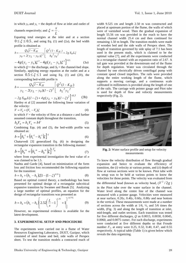
width 9.525 cm and length 2.50 m was constructed and placed at upstream portion of the flume, the walls of which were of varnished wood. Then the gradual expansion of length 55.56 cm was provided in the reach to have the normal channel width 25.4 cm and then continued for remaining 1.50 m length. The transition models were made of wooden bed and the side walls of Perspex sheet. The length of transition governed by side splay of 7:1 has been used in the present study, which is claimed to be the optimal value [7], and all the experiments were conducted in a rectangular channel with an expansion ratio of 2.67. A tail gate was provided at the downstream end of the flume for depth regulation. Water was circulated through the channel by one electrically driven centrifugal pump with constant speed closed impellers. The rails were provided along the entire working length of the flume, which supports a moving carriage, and a continuous scale calibrated in millimeters is provided along the length of one of the rails. The carriage with pointer gauge and Pitot tube is used for depth of flow and velocity measurements respectively (Fig. 2). (3b)

Fig. 2: Water surface profile and setup for velocity measurements

To know the velocity distribution of flow through gradual expansion and hence to evaluate the efficiency of transition, the (i) velocity at various points, and (ii) depth of flow at various sections were to be known. Pitot tube with its setup was to be held at various points to know the velocities for those points. The velocity was evaluated from the differential head (known as velocity head, ( ) in the Pitot tube over the water surface in the channel. Water level along the centre line of the channel was measured with a pointer gauge. Velocities were measured at near surface, 0.20y, 0.40y, 0.60y, 0.80y and near bottom in the vertical. These measurements were made at a number of sections across the width at 1/6, ½, and 5/6 times the width, (Fig. 3) and along the length of transition at inlet, mid-length, and outlet sections. Each transition was tested for five different discharges, Q as 0.0015, 0.0030, 0.0045, 0.0060, and 0.0075 cumec. For each discharge, experiments were conducted at five different depths so that Froude number F

gV 2/2

1, at entry were 0.25, 0.32, 0.40, 0.47, and 0.55 respectively. A typical table (Table 1) is given below which reveals the data organizing.



Table 1: Local velocity (Model IV, Q = 0.0045 cumec) 4. BACKGROUND OF EFFICIENCY For finding the efficiency, it is necessary to consider the velocity variation across the channel. Referring to section 1-1 at the inlet, Fig. 3, let v be the velocity of flow through an infinitesimal area dA. Assuming that the flow is essentially in the direction of the axis of the transition, the volume of fluid per unit time passing through the elementary area is vdA, and then the mass rate of flow through this area is ρvdA. The kinetic energy of this fluid

mass per unit time is ( ) 2

21 vvdAρ , or dAv3

21 ρ . The total

Inlet tank Perspex sheet sidewall

kinetic energy per unit time passing over the entire section

1-1, is obtained by integrating the term dAv3

21 ρ , i.e.,

dAvA∫

1

3

21 ρ , where A1 indicates integration over the cross-

section 1-1. In a similar manner, the kinetic energy per unit time for section 2-2, at the outlet of transition is

dAvA∫

2

3

21 ρ . As the fluid passes through the transition, the

actual reduction in kinetic energy per unit time, or the power available for transformation in the transition, is the

difference of the above two, i.e., dAvdAvAA ∫∫ −

21

33

21

21 ρρ .

All of this energy is not transformed into useful work. It may be helpful to imagine the transition as a pump. The pump raises the pressure of the fluid entering. The term

dAvdAvAA ∫∫ −

21

33

21

21 ρρ might be regarded as the power

supplied or input to the pump. The head gained by the fluid flowing through the transition is ( , where y)12 yy − 1 and y2 refer to the depths of flow at sections 1-1 and 2-2 respectively. If Q be the rate of flow per sec, potential energy gained by the fluid per sec will be ( )12 yygQ −ρ which gives the actual power, the pump adds to the fluid. The purpose of transition is to convert kinetic energy into useful pressure energy. Hence, the efficiency of the transition is defined by

( )

∫ ∫−

−=

1 2

33

12

21

21

A AdAvdAv

yygQ

ρρ

ρε (10)

Fig. 3: Top view of flume with the section showing the various points of velocity measurements

Q m3/s F 1

y 1 at inlet mm

∆ y 1, mm

y 2 at outlet mm

∆ y 2, mm

y 3 at L /4 mm

y 4 at L /2 mm

y 5 at 3L /4 mm

0.25 153.0 30.6 155.3 31.1 153.8 154.3 154.80.32 129.0 25.8 131.5 26.3 130.0 130.8 131.40.4 110.0 22.0 114.2 22.8 111.3 112.3 113.20.47 101.0 20.2 105.4 21.1 102.8 104.3 105.00.55 89.0 17.8 94.8 19.0 91.0 92.8 94.0

0.0045

Reading, h in mm

Velocity, v in

m/sec

Reading, h in mm

Velocity, v in

m/sec

Reading, h in mm

Velocity, v in

m/sec

Reading, h at 0.6y4,

mm

Avg. Vel, v in m/sec

0.1 y 10.0 0.443 10.5 0.454 10.0 0.4430.2 y 10.5 0.454 11.0 0.465 10.5 0.4540.4 y 10.0 0.443 10.5 0.454 10.0 0.4430.6 y 9.0 0.420 9.5 0.432 9.0 0.420 3.0 0.2430.8 y 8.0 0.396 8.5 0.408 7.5 0.384 5.5 0.3280.9 y 6.0 0.343 7.0 0.371 6.0 0.343 5.5 0.3280.1 y 5.0 0.313 6.0 0.343 2.5 0.221 4.5 0.2970.2 y 6.5 0.357 7.5 0.384 3.0 0.243 2.5 0.2210.4 y 6.0 0.343 6.5 0.357 2.5 0.2210.6 y 3.0 0.243 4.0 0.280 1.5 0.172 4.5 0.2970.8 y 1.0 0.140 2.0 0.198 1.0 0.140 4.0 0.2800.9 y 0.0 0.000 0.0 0.000 0.0 0.000

V. at mid-length

0.4

Inlet

Outlet at b /3, and 2b /3 at I/O

Frou

de

No.

, F1

Sect

ion At

Depths

At b /6 At b /2 At 5b /6

b) Cross-section at inlet of transition model with various points of measurements

b/6 b/2 5b/6 Near surface

0.2 y

0.4 y

0.8 y

Near bottom

Bed width, b

Flow depth, y

Transition model Control weir

Outflow

Wooden channel Inlet transition 1

250 cm 35 cm 65 cm 55.56 cm 150 cm

2

25.4 cm 9.525 cm

a) Top view of flume

0.6 y



Suppose, be the average velocity at section 1-1 and be the average velocity at section 2-2. Then one can write

1V 2V

12

13

21

21

1

αρρ ⎟⎠⎞

⎜⎝⎛=∫ QVdAv

A (11)

and

22

13

21

21

2

αρρ ⎟⎠⎞

⎜⎝⎛=∫ QVdAv

A (12)

where, 1α and 2α are numerical constants, known as energy coefficients for non-uniformity of velocity distribution. Now Eq. (10) takes the form

( ) ( )

⎟⎟⎠

⎞⎜⎜⎝

⎛−

−=

⎟⎠⎞

⎜⎝⎛−⎟

⎠⎞

⎜⎝⎛

−=

gV

αg

Vα

yy

αρQVαQV

yygQε

2221

21 2

22

21

1

12

22

212

1

12

ρ

ρ (13)

The energy coefficients, 1α and 2α are obtained numerically from Eqs. (11) and (12). 5. ANALYSIS OF DATA The velocities measured at different depths in the vertical indicated the usual turbulent boundary layer profile (mentioned in data table); as such, only the average velocity over a vertical was used in further analysis. Using the data for depth of flow and local velocity, the flow area and average velocity at the sections were known, and thus energy correction factors were calculated. After then these data were used to evaluate the efficiency of transition from the expression shown above. The table (Table 2) given below shows this in brief. Four transition profiles used commonly in the field [2, 3, 4 and 5], are tested for performance and compared the efficiency of the models, i.e. Model I, II, III, and IV respectively.

Table 2: Average velocity, energy correction factor, and efficiency (Model IV, Q = 0.0045 cumec)

The percentage efficiencies for different discharges and Froude numbers, and also overall efficiencies of the transition models are presented in Table 3a. The efficiencies of the transition models for average of discharges and average of Froude numbers are also summarized in Table 3b, where the comparative feature of performance of the models is observed. The efficiency

Table 3a: Overall hydraulic efficiencies of the transition models

Table 3b: Hydraulic efficiencies of the transition models (for avg. of Q and avg. of F1)

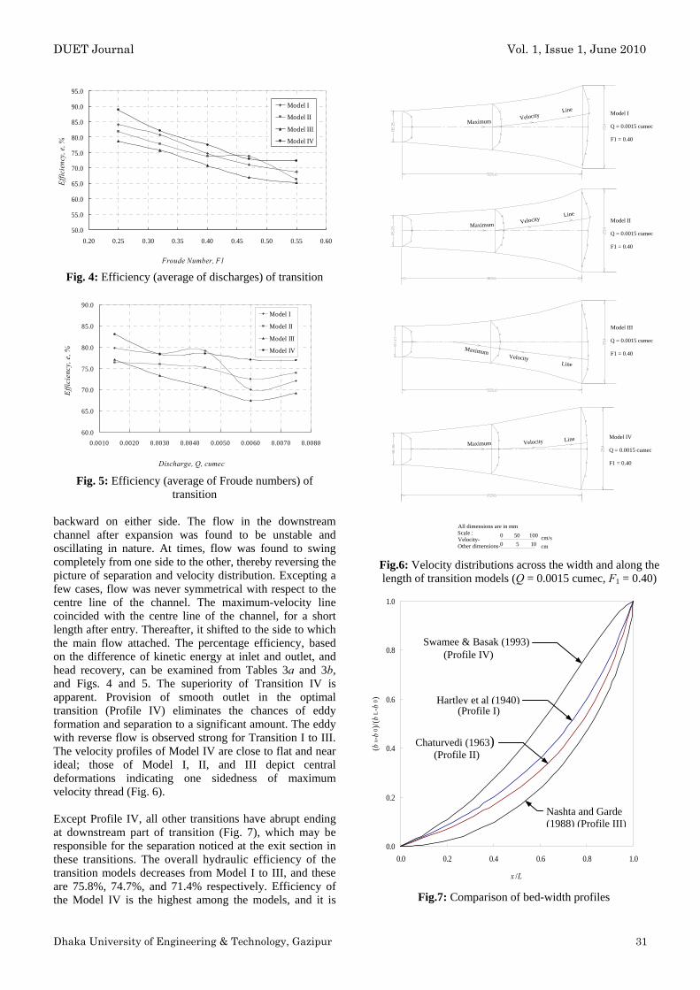
curves for average of discharges and for average of Froude numbers for the four models have been shown in Figs. 4 and 5, respectively. 6. EXPERIMENTAL OBSERVATION AND

RESULTS The surface configuration in the transitions I, II, and III exhibited local disturbances leading to diagonal waves, starting in the inlet section and persisting towards the entire length of the transition. The separation of flow took place at the boundaries near the exit of the transition. The points of separation were not symmetrical on either side; this was also observed by several investigators earlier. The separation points were found to move forward and

Avg. Vel., v ∆y v ∆y

Avg. V / strip

Avg. V / Section v 3∆y

α / Strip

α / Section

Efficiency,ε , %

0.448 0.0220 0.010 0.00200.448 0.0220 0.010 0.00200.432 0.0220 0.009 0.00180.408 0.0220 0.009 0.00150.370 0.0220 0.008 0.00110.459 0.0220 0.010 0.00210.459 0.0220 0.010 0.00210.443 0.0220 0.010 0.00190.420 0.0220 0.009 0.00160.389 0.0220 0.009 0.00130.448 0.0220 0.010 0.00200.448 0.0220 0.010 0.00200.432 0.0220 0.009 0.00180.402 0.0220 0.009 0.00140.363 0.0220 0.008 0.00110.335 0.0228 0.008 0.00090.350 0.0228 0.008 0.00100.293 0.0228 0.007 0.00060.191 0.0228 0.004 0.00020.070 0.0228 0.002 0.00000.363 0.0228 0.008 0.00110.370 0.0228 0.008 0.00120.319 0.0228 0.007 0.00070.239 0.0228 0.005 0.00030.099 0.0228 0.002 0.00000.232 0.0228 0.005 0.00030.232 0.0228 0.005 0.00030.197 0.0228 0.004 0.00020.156 0.0228 0.004 0.00010.070 0.0228 0.002 0.0000

Outlet

Strip I 0.248

0.234Strip II 0.278

Strip III 0.177

0.425

1.02

1.01

76.2

1.01

1.02

1.49

1.391.36

1.32

Section

Inlet

Strip I 0.421

Strip II 0.434

Strip III 0.419

0.25 87.8 84.2 80 89.20.32 82.8 70.3 83.8 890.4 78.4 75.5 80.9 80.90.47 73.4 79.1 68.6 76.70.55 76.4 72.7 71.9 790.25 88.1 77.8 78.1 87.10.32 83 80 72.8 77.70.4 79.3 76.5 70.8 78.70.47 70.1 76.6 74 76.40.55 71.4 68.9 70.4 71.70.25 85.6 84.7 80.7 92.70.32 86.6 81.3 75.9 78.10.4 77.6 74.4 68.9 76.20.47 77.3 69.8 65.7 72.40.55 68.2 65.3 61.2 72.90.25 80 81.2 76.6 86.70.32 76 75.3 74.3 80.40.4 70.2 72.1 67 77.60.47 64.6 72.2 59 71.10.55 59.1 61.3 59.8 69.30.25 78.8 81.7 77.8 88.10.32 74.8 82.4 71.7 85.50.4 68.3 70.7 66.2 73.80.47 69.5 70.9 67.2 67.90.55 68.7 63.8 62.5 68.9

78.7

0.002

75.8 74.7 71.4

.003

.005

.006

.008

Model III Model IV

Efficiency, ε , %

Overall Efficiency,

ε , %

Efficiency ε , %

Overall Efficiency

ε , %Dis

char

ge,

Q, c

umec

Frou

de N

o.,

F1

Model I Model II

Efficiency ε , %

Overall Efficiency

ε , %

Efficiency, ε , %

Overall Efficiency,

ε , %

0

0

0

0

forAvg. Q

for Avg.F 1

forAvg. Q

for Avg.F 1

for Avg.Q

forAvg.

for Avg.Q

for Avg.F 1

0.25 84.1 81.9 78.6 88.80.320.4

80.6 77.9 75.7 82.10 74.8 73.8 70.8 77.4

71.0 73.7 66.9 72.968.8 66.4 65.2 72.4

0.002 79.8 76.4 77.0 83.00.003 78.

0.470.55

4 76.0 73.2 78.30.005 79.1 75.1 70.5 78.50.006 70.0 72.4 67.3 77.00.008 72.0 73.9 69.1 76.8

Frou

deNo

., F

1

Disc

harg

e,Q

, cum

ec Model I Model II Model III Model IVAverage Efficiency Average EfficiencyAverage EfficiencyAverage Efficiency



50.0

55.0

60.0

65.0

70.0

75.0

80.0

85.0

90.0

95.0

0.20 0.25 0.30 0.35 0.40 0.45 0.50 0.55 0.60

Froude Number, F1

Effic

ienc

y, e

, %

Model I

Model II

Model III

Model IV

Fig. 4: Efficiency (average of discharges) of transition

60.0

65.0

70.0

75.0

80.0

85.0

90.0

0.0010 0.0020 0.0030 0.0040 0.0050 0.0060 0.0070 0.0080

Discharge, Q, cumec

Effic

ienc

y, e

, %

Model I

Model II

Model III

Model IV

Fig. 5: Efficiency (average of Froude numbers) of

transition backward on either side. The flow in the downstream channel after expansion was found to be unstable and oscillating in nature. At times, flow was found to swing completely from one side to the other, thereby reversing the picture of separation and velocity distribution. Excepting a few cases, flow was never symmetrical with respect to the centre line of the channel. The maximum-velocity line coincided with the centre line of the channel, for a short length after entry. Thereafter, it shifted to the side to which the main flow attached. The percentage efficiency, based on the difference of kinetic energy at inlet and outlet, and head recovery, can be examined from Tables 3a and 3b, and Figs. 4 and 5. The superiority of Transition IV is apparent. Provision of smooth outlet in the optimal transition (Profile IV) eliminates the chances of eddy formation and separation to a significant amount. The eddy with reverse flow is observed strong for Transition I to III. The velocity profiles of Model IV are close to flat and near ideal; those of Model I, II, and III depict central deformations indicating one sidedness of maximum velocity thread (Fig. 6). Except Profile IV, all other transitions have abrupt ending at downstream part of transition (Fig. 7), which may be responsible for the separation noticed at the exit section in these transitions. The overall hydraulic efficiency of the transition models decreases from Model I to III, and these are 75.8%, 74.7%, and 71.4% respectively. Efficiency of the Model IV is the highest among the models, and it is

All dimensions are in mmScale :Velocity-Other dimensions-

MaximumModel IV

Q = 0.0015 cumec

F1 = 0.40

0 50 50

cm10cm/s100

Velocity Line

Maximum

Maximum

MaximumModel I

Q = 0.0015 cumec

F1 = 0.40

Model III

Q = 0.0015 cumec

F1 = 0.40VelocityLine

Model II

Q = 0.0015 cumec

F1 = 0.40

VelocityLine

VelocityLine

(

F

x -0 )

/(L

-0 )

bb

bb

Dhaka University of Engineering & Technology, Gazipur

ig.6: Velocity distributions across the width and along thelength of transition models (Q = 0.0015 cumec, F = 0.40)

0.0

0.2

0.4

0.6

0.8

1.0

0.0 0.2 0.4 0.6 0.8 1.0

x /L

1

Swamee & Basak (1993) (Profile IV)

Hartley et al (1940) (Profile I)

Chaturvedi (1963) (Profile II)

Nashta and Garde (1988) (Profile III)

Fig.7: Comparison of bed-width profiles

31


78.7%. Abrupt ending in the transition profiles evolved by Hartley et al [2], Chaturvedi [3], and Nashta and Garde [4], shifts the efficiency curves (Figs. 4 and 5) downward, whereas smooth ending in the optimal transition (Profile IV) makes it efficient over others, and keeps the efficienccurve at top. Figure 8 shows the overall hydraulic efficiency of the various transition profiles, where dominance of the Profile IV is observed over others.

y iii.

7. CONC In the ligcould be i. Th

prproth

ii. ThMwi

flow decreases, the local velocity remains considerably high, which if allowed to persist in erodible channels will scour away bed and sides of channel.

REFERENCES

[1] J. Hinds, “The hydraulic design of flume and siphon transitions,” Trans., ASCE, 92, pp. 1423-1459, 1928.

[2] G. E. Hartley, J. P. Jain and A. P. Bhattacharya, “Report

on the model experiments of fluming of bridges on Purwa branch,” Technical Memorandum. 9, United Provinces Irrigation Res. Inst., Lucknow (now at Roorkee), India, pp. 94-110, 1940.

[3] R. S. Chaturvedi, “Expansive subcritical flow in open

channel transitions,” J. Inst. of Engrs., India, 43(9), pp. 447-487, 1963.

60.062.064.066.068.070.072.074.076.078.080.0

Model I Model II Model III Model IV

F

Effic

ienc

y, ε

, %

Dhaka U

ig.8: Efficiency of the Transition Models

LUSIONS

ht of the present study the following conclusions drawn:

e Transition Profile IV yields a design that oduces the highest efficiency among the existing ofiles. So, this can be suggested for field use over ers. e velocity distribution after expansion in case of odel I, II, and III becomes highly non-uniform th the result that although the average velocity of

[4] C. F. Nashta, and R. J. Garde, “Subcritical flow in

rigid-bed open channel expansions,” J. Hydr. Res., 26(1), pp. 49-65, 1988.

[5] P. K. Swamee and B. C. Basak, “A comprehensive

open-channel expansion transition design,” J. of Irrg. and Drainage Div., ASCE, 119(1), pp. 1-17, 1993.

[6] H. M. Morris and J. M. Wiggert, Applied Hydraulics in Engineering. Second Ed., The Ronald Press Co., New York, N. Y., 1972, pp. 184-188.

[7] S. K. Mazumder, “Optimum length of transition in open channel expansive subcritical flow,” J. Inst. of Engrs., India, 48(3), pp. 463-478, 1967.

niversity of Engineering & Technology, Gazipur 32

Efficiency of an Expansive Transition in an Open Channel ...

Documents

Transcript of Efficiency of an Expansive Transition in an Open Channel ...