Effects of the Kinematic Model on Forward-Model Based ...
71
Wright State University Wright State University CORE Scholar CORE Scholar Browse all Theses and Dissertations Theses and Dissertations 2017 Effects of the Kinematic Model on Forward-Model Based Effects of the Kinematic Model on Forward-Model Based Spotlight SAR ECM Spotlight SAR ECM David T. Pyles Wright State University Follow this and additional works at: https://corescholar.libraries.wright.edu/etd_all Part of the Electrical and Computer Engineering Commons Repository Citation Repository Citation Pyles, David T., "Effects of the Kinematic Model on Forward-Model Based Spotlight SAR ECM" (2017). Browse all Theses and Dissertations. 1864. https://corescholar.libraries.wright.edu/etd_all/1864 This Thesis is brought to you for free and open access by the Theses and Dissertations at CORE Scholar. It has been accepted for inclusion in Browse all Theses and Dissertations by an authorized administrator of CORE Scholar. For more information, please contact [email protected].
Transcript of Effects of the Kinematic Model on Forward-Model Based ...

Wright State University Wright State University
CORE Scholar CORE Scholar
Browse all Theses and Dissertations Theses and Dissertations
2017
Effects of the Kinematic Model on Forward-Model Based Effects of the Kinematic Model on Forward-Model Based
Spotlight SAR ECM Spotlight SAR ECM
David T. Pyles Wright State University
Follow this and additional works at: https://corescholar.libraries.wright.edu/etd_all
Part of the Electrical and Computer Engineering Commons
Repository Citation Repository Citation Pyles, David T., "Effects of the Kinematic Model on Forward-Model Based Spotlight SAR ECM" (2017). Browse all Theses and Dissertations. 1864. https://corescholar.libraries.wright.edu/etd_all/1864
This Thesis is brought to you for free and open access by the Theses and Dissertations at CORE Scholar. It has been accepted for inclusion in Browse all Theses and Dissertations by an authorized administrator of CORE Scholar. For more information, please contact [email protected].
Effects of the Kinematic Model on Forward-ModelBased Spotlight SAR ECM
A Thesis submitted in partial fulfillmentof the requirements for the degree of
Master of Science in Electrical Engineering
by
David T. PylesB.S.E.E., Wright State University, 2016
2017Wright State University

Wright State UniversityGRADUATE SCHOOL
January 2, 2018
I HEREBY RECOMMEND THAT THE THESIS PREPARED UNDER MY SUPER-VISION BY David T. Pyles ENTITLED Effects of the Kinematic Model on Forward-ModelBased Spotlight SAR ECM BE ACCEPTED IN PARTIAL FULFILLMENT OF THE RE-QUIREMENTS FOR THE DEGREE OF Master of Science in Electrical Engineering.
Michael A. Saville, Ph.D., P.E.Thesis Director
Brian D. Rigling, Ph.D.Chair, Department of Electrical Engineering
Committee onFinal Examination
Michael A. Saville, Ph.D., P.E.
Brian D. Rigling, Ph.D.
Steve Gorman, Ph.D.
Barry Milligan, Ph.D.Interim Dean of the Graduate School
ABSTRACT
Pyles, David T. M.S.E.E., Department of Electrical Engineering, Wright State University, 2017.Effects of the Kinematic Model on Forward-Model Based Spotlight SAR ECM.
Spotlight synthetic aperture radar (SAR) provides a high-resolution remote image-
formation capability for airborne platforms. SAR image formation processes exploit the
amplitude, time, and frequency shifts that occur in the transmitted waveform due to elec-
tromagnetic propagation and scattering. These shifts are predictable through the SAR for-
ward model which is dependent on the waveform parameters and emitter flight path. The
approach to develop an electronic countermeasure (ECM) system that is founded on the
SAR forward model implies that the ECM system should alter the radar’s waveform in a
manner that produces the same amplitude, time, and frequency shifts that a real scatterer
would produce at a desired location. A collection of such scatterers would be capable of
forming a larger collective energy distribution in the final image. However, since the for-
ward model is dependent on the radar platform’s kinematic model, the jamming energy
distribution created from a forward-model based ECM system will inherently have some
level of sensitivity to kinematic error. This thesis discusses a forward-model based ECM
modulation scheme and provides an assessment of its sensitivity through Monte Carlo sim-
ulations and an entropy-based image similarity distance.
iii

Contents
1 Introduction 11.1 Overview . . . . . . . . . . . . . . . . . . . . . . . . . . . . . . . . . . . 11.2 Challenges . . . . . . . . . . . . . . . . . . . . . . . . . . . . . . . . . . . 21.3 Hypothesis . . . . . . . . . . . . . . . . . . . . . . . . . . . . . . . . . . 21.4 Outline . . . . . . . . . . . . . . . . . . . . . . . . . . . . . . . . . . . . 3
2 Background 42.1 Literature Review . . . . . . . . . . . . . . . . . . . . . . . . . . . . . . . 42.2 Spotlight SAR Theory . . . . . . . . . . . . . . . . . . . . . . . . . . . . 5
2.2.1 Kinematic and Processing Model . . . . . . . . . . . . . . . . . . 72.2.2 Phase Analysis . . . . . . . . . . . . . . . . . . . . . . . . . . . . 112.2.3 K Error, Moving Targets, and Auto-Focus . . . . . . . . . . . . . . 13
2.3 ECM Development . . . . . . . . . . . . . . . . . . . . . . . . . . . . . . 152.4 Summary . . . . . . . . . . . . . . . . . . . . . . . . . . . . . . . . . . . 20
3 Methodology 213.1 Proposed Study . . . . . . . . . . . . . . . . . . . . . . . . . . . . . . . . 213.2 Experiment Procedure . . . . . . . . . . . . . . . . . . . . . . . . . . . . 22
3.2.1 Emitter Model . . . . . . . . . . . . . . . . . . . . . . . . . . . . 233.2.2 Monte Carlo Accuracy . . . . . . . . . . . . . . . . . . . . . . . . 243.2.3 Image Similarity Metric . . . . . . . . . . . . . . . . . . . . . . . 25
4 Results 284.1 Use Case Example . . . . . . . . . . . . . . . . . . . . . . . . . . . . . . 33
5 Conclusion 36
Bibliography 37
Appendix A Information Bounds and Waveform Parameters 41
Appendix B Linear Frequency Modulated Waveform Considerations 46
iv

Appendix C SAR Processing Model 49
Appendix D Jaccard Distance Examples 52
Appendix E Linear Frequency Modulated Waveform Model and Processing 55
v
List of Figures
2.1 Illumination grid on the scene. Each isorange contour r′ follows the groundat a constant range r from the emitter. In spotlight SAR mode the centralreference point (CRP) remains constant. . . . . . . . . . . . . . . . . . . . 6
2.2 General data processing model. . . . . . . . . . . . . . . . . . . . . . . . . 82.3 DMF result for a bed-of-nails scene. The radar kinematic and waveform
parameters are provided in Tab. 2.1. . . . . . . . . . . . . . . . . . . . . . 102.4 DMF result for a bed-of-nails scene with a 5 percent error in the range
estimate. . . . . . . . . . . . . . . . . . . . . . . . . . . . . . . . . . . . . 112.5 The change in range and cross-range contours for two different points of
a flight path. With a pulse transmitted at each angle, the target resides ondifferent range and cross-range contours, resulting in a change in phase. . . 12
2.6 Ideal phase arguments with x = 10 km, y from −500 : 500 m, similar toFig. 2.5, and radar parameters consistent with Tab. 2.1. . . . . . . . . . . . 13
2.7 Ideal phase arguments with an estimation error of x = Est×X , where Estis the scale factor listed in the legend. The radar parameters used here arethe same as used for Fig. 2.6. . . . . . . . . . . . . . . . . . . . . . . . . . 15
2.8 Illumination grid geometry. The radar is located at (xr, yr) moving in a +ydirection, the jammer is at (xJ , yJ ), and the desired false target displace-ment is some (∆x1,∆y1) from the jammer and some angle θ from the +yvelocity vector of the radar. . . . . . . . . . . . . . . . . . . . . . . . . . . 17
4.1 a) Simulation scene. As the radar travels in the positive cross-range direc-tion, a pulse echoes from the ECM Location along a blue line. The ECMsystem alters the waveform such that the data resembles a pulse return fromthe false target location along the appropriate path, shown as a red line. b)The range history of both the ECM system and the false target. This rangehistory is equivalent to the length of the red and blue lines in (a) for eachpulse. . . . . . . . . . . . . . . . . . . . . . . . . . . . . . . . . . . . . . 29
4.2 Top: Upper 60 dB of comparison image generated with no noise and anideal K. Bottom: Upper 30 dB of local energy distribution region of thecomparison image. . . . . . . . . . . . . . . . . . . . . . . . . . . . . . . 29
4.3 Jaccard estimates for noise-only error. 1000 Monte Carlo trials were runfor each SNR. . . . . . . . . . . . . . . . . . . . . . . . . . . . . . . . . . 30
vi
4.4 Calculated number of trials required to meet the specified confidence levelfor the velocity and location random variables required to acheive a 98%confidence level that the result is within 4% of the true average, accordingto Eq. (3.6). . . . . . . . . . . . . . . . . . . . . . . . . . . . . . . . . . . 31
4.5 Average Jaccard distance versus standard deviation in velocity (V), range(X), and cross-range (Y) for the specified N trials. . . . . . . . . . . . . . . 32
4.6 Select example results in range (X) dimension.a) Left: DMF result of σx = 0.1172 m, Jaccard = 0.0777. Right: Zoomedand scaled version of left image.b) Left: DMF result of σx = 1.2690 m, Jaccard = 0.4281. Right: Zoomedand scaled.c) Left: DMF result of σx = 4.1750 m, Jaccard = 0.7829. Right: Zoomedand scaled.d) Left: DMF result of σx = 67.2336 m, Jaccard = 0.9919. Right: Zoomedand scaled, note that the distribution resides near the scene extent. . . . . . 34
4.7 Select example results in range (Y) dimension.a) Left: DMF result of σy = 0.1172 m, Jaccard = 0.0534. Right: Zoomedand scaled version of left image.b) Left: DMF result of σy = 1.2690 m, Jaccard = 0.3941. Right: Zoomedand scaled.c) Left: DMF result of σy = 4.1750 m, Jaccard = 0.6485. Right: Zoomedand scaled.d) Left: DMF result of σy = 67.2336 m, Jaccard = 0.9806. Right: Zoomedand scaled, note that the distribution resides near the scene extent. . . . . . 35
A.1 One projection samples the illuminated area in a polar format. Range iscalculated based the on time delay from the center Doppler line. Cross-range is mapped through the phase measurements for each isorange delay. . 42
A.2 A collection of slices in Fourier space. The annulus represents the skewedimage K-space in the form of Doppler shifts, centered vertically on fr atγ = 4πfc/c. Note that only the shaded portion of each slice is collecteddue to the bandlimited nature of radars. . . . . . . . . . . . . . . . . . . . 43
A.3 Range gate example, data is only collected during the desired time windowtw. . . . . . . . . . . . . . . . . . . . . . . . . . . . . . . . . . . . . . . . 44
A.4 Tw bounds for range gating based on desired scene size Lx, x0 = 10 km. . . 45
B.1 Effective bandwidth extents for a given scene size (LxxLy). Note that βeffis equivalent to twice the max fd deviation from fc. x0 = 10 km, v =340.29 m/s, fc = 10 GHz, and θc = π/4 rad. . . . . . . . . . . . . . . . . . 47
B.2 Effective bandwidth extents for a given scene size (LxxLy) and LFM wave-form. The same parameters were used here as for Fig. B.1, along with aPW = 10 us, and K = 50 MHz/us. . . . . . . . . . . . . . . . . . . . . . 48
D.1 Translational and rotational affect on the normalized Jaccard Distance forthe top image. . . . . . . . . . . . . . . . . . . . . . . . . . . . . . . . . . 53
vii

D.2 Monte Carlo result histogram of the Jaccard Distance between an image Aand B = A+ n, where n ∼ N (0, .022) w.g.n. for 1000 trials. . . . . . . . . 54
E.1 Relative velocity model. . . . . . . . . . . . . . . . . . . . . . . . . . . . 59
viii

AcknowledgmentFirst and foremost I am grateful to God for the many blessing given while completing
this work. I wish to express my sincere gratitude to Cornelius for providing a unique
perspective of the remote imaging field and for guiding my foundational learning in the
area. I also thank my advisor Dr. Saville for helping to make this thesis what it is, and
thank Dr. Rigling and Dr. Gorman for serving on my thesis committee.
ix

Dedicated to my amazing wife, Emily.
x
Introduction
1.1 Overview
Spotlight synthetic aperture radar (SAR) allows for remote formation of high-resolution
images of a localized area of the earth. This mode is facilitated by a radar carried by
an aerial vehicle that illuminates the desired area for some amount of time and collects
backscatter signals from different angles. SAR image formation processes (IFP) exploit
the amplitude, time, and frequency shifts that occur in the transmitted waveform due to
electromagnetic propagation and scattering. The magnitude and hysteresis of each shift is
dependent on the relative kinematics between the emitter and the scene, which is observed
through analysis of the forward model. The approach to develop an electronic counter-
measure (ECM) system that is founded on the SAR forward model implies that the ECM
system should alter the radar’s waveform in a manner that produces the same amplitude,
time, and frequency shifts that a real scatterer would produce. This approach increases
confidence that the ECM waveform results in the desired energy distribution in the final
image regardless of the waveform or IFP utilized by the SAR system. However, since the
forward model is dependent on the radar platform’s kinematic model, the jamming energy
distribution created from a forward-model based ECM system will inherently have some
level of sensitivity to kinematic error. This thesis discusses a forward-model based ECM
modulation scheme and provides an assessment of its sensitivity through Monte Carlo trials
and image similarity calculations.
1
1.2 Challenges
A major challenge of SAR ECM development is the complex dependency of the time-
variant geometry between the radar, the ECM platform, and the illuminated scene. In
this work, the SAR ECM system is assumed to have the capability to determine a SAR
platform’s location and trajectory to some degree of accuracy. The SAR ECM system is
assumed to have basic digital radio frequency memory (DRFM) capabilities, which include
the capability to record the waveform transmitted by the radar, perform basic signal pro-
cessing tasks to the data, and transmit a response waveform at a power level sufficient to
achieve a jamming-to-signal ratio of one [1, 2, 3]. Also, the radar’s IFP and the utilization
of auto-focus techniques are expected to be unknown to the ECM system, which may blur
the intended energy distribution in an undesirable manner. There are numerous other chal-
lenges, such as ECM technique effectiveness assessments, but they are specific to an ECM
technique and are not considered here. Also any multi-path effects are ignored.
1.3 Hypothesis
SAR IFPs are fundamentally dependent on an estimate of the geometric relationship of
the antenna and the illuminated area in order to exploit the amplitude, time, and frequency
shifts that are present in the received waveform to produce a facsimile of the scene. There-
fore, the hypothesis presented is that the quality of the resulting jamming energy distribu-
tion in a spotlight SAR processed image is limited by the accuracy of the forward-model
based ECM system’s estimation of the radar platform’s kinematic model.
2
1.4 Outline
The development approach for SAR ECM in this work is inspired by recent literature on
the subject. Following the primary assumptions often presented in other works, Chapter
2 discusses spotlight SAR theory and presents the forward model with a linear-frequency
modulated (LFM) signal model. Chapter 2 continues with kinematic and general SAR-
processing models which explain how the scene is estimated from the collected waveform
data and results in an image. Phase analysis of the LFM signal model is then used to
express the forward model in a manner which clearly exposes the kinematic relationships.
The spotlight SAR theory section concludes by discussing common errors in SAR IFPs and
the effects of moving targets.
The second half of Chapter 2 discusses general ECM theory with a focus on an ECM
system’s required knowledge of the radar’s kinematic model in order to control a jamming
energy distribution. ECM waveform design is assessed as an extension of the SAR phase
analysis in order to identify a forward-model based modulation scheme that a DRFM may
utilize in order to embed the ECM user’s desired false target information into the returned
waveform.
Chapter 3 presents the methodology that is followed in order to assess the sensitivity
of the jamming energy point spread function to errors in the ECM system’s kinematic
estimate. This includes a discussion of Monte Carlo trial accuracy and the Jaccard Distance.
Finally, chapter 4 presents the results of the experiment detailed in chapter 3.
3
Background
2.1 Literature Review
SAR ECM has been studied from multiple perspectives. The authors of [4] approached
noise and deception jamming requirements with respect to effective radiated power levels
with the assumption that the jammer has knowledge of the radar’s location, timing, and
waveform details. In [5], the authors analyzed noise jamming techniques against a general
SAR ground moving target indicator process and determined the necessary jamming-to-
signal ratio required for noise jamming to effectively hide a moving target’s Doppler shift.
The authors of [6] studied active deception jamming for a single false target, multiple false
targets, and scene generation. In [7], the authors provided an analysis of the effects on
inverse SAR jamming through sinusoidal phase modulation. The authors of [8] provided
an ECM signal generation method to counter space-born SAR emitters through parallel
computing. In [9], the authors demonstrated SAR ECM jamming through the utilization of
micro-Doppler perturbations, which result in vibrating-target effects [16]. In [26] and [27]
the authors present a DRFM-based image generation method which utilize individual false
targets to create a jamming image. These studies provide much in regards to ECM tech-
niques, however their effectiveness may be limited due to the emitter’s unknown or poorly
estimated flight path and possible use of auto-focus. While many studies assume a straight
emitter flight path in order to simplify analysis, in practice the estimates of a flight path
distort the intended ECM energy distribution.
4
2.2 Spotlight SAR Theory
Spotlight SAR systems persistently illuminate a local area and exploit the properties of
electromagnetic propagation and scattering to form images from the amplitude, time, and
frequency shifts of the microwave spectrum. The scattering of a pulse p from the scene
reflects back some portion of the pulse’s energy which is determined by the scene’s reflec-
tivity density ρ at time t. A 2-dimensional estimate of ρ is formed by the radar from the
1-dimensional collection of pulse returns [11]. Each scatterer reflects back the transmitted
waveform with amplitude, time, and frequency shifts unique to that scatterer’s reflectiv-
ity density and location. To demonstrate, allow the mth LFM pulse transmitted from the
emitter to be modeled as
sTx(t−mPRI) = A0p(t−mPRI)ej2πfc(t−mPRI)+jπk(t−mPRI)2 , (2.1)
where A0 is the pulse amplitude, fc is the carrier frequency, PRI is the pulse repetition
interval, M is the number of pulses, k is the frequency-modulation factor, and time t is
proportional to range r through the standard range equation
t =2r
c, (2.2)
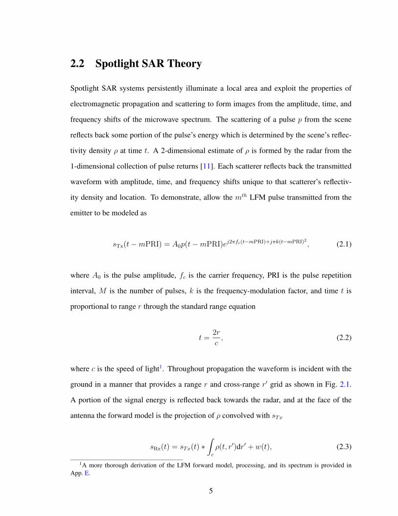
where c is the speed of light1. Throughout propagation the waveform is incident with the
ground in a manner that provides a range r and cross-range r′ grid as shown in Fig. 2.1.
A portion of the signal energy is reflected back towards the radar, and at the face of the
antenna the forward model is the projection of ρ convolved with sTx
sRx(t) = sTx(t) ∗∫c
ρ(t, r′)dr′ + w(t), (2.3)
1A more thorough derivation of the LFM forward model, processing, and its spectrum is provided inApp. E.
5
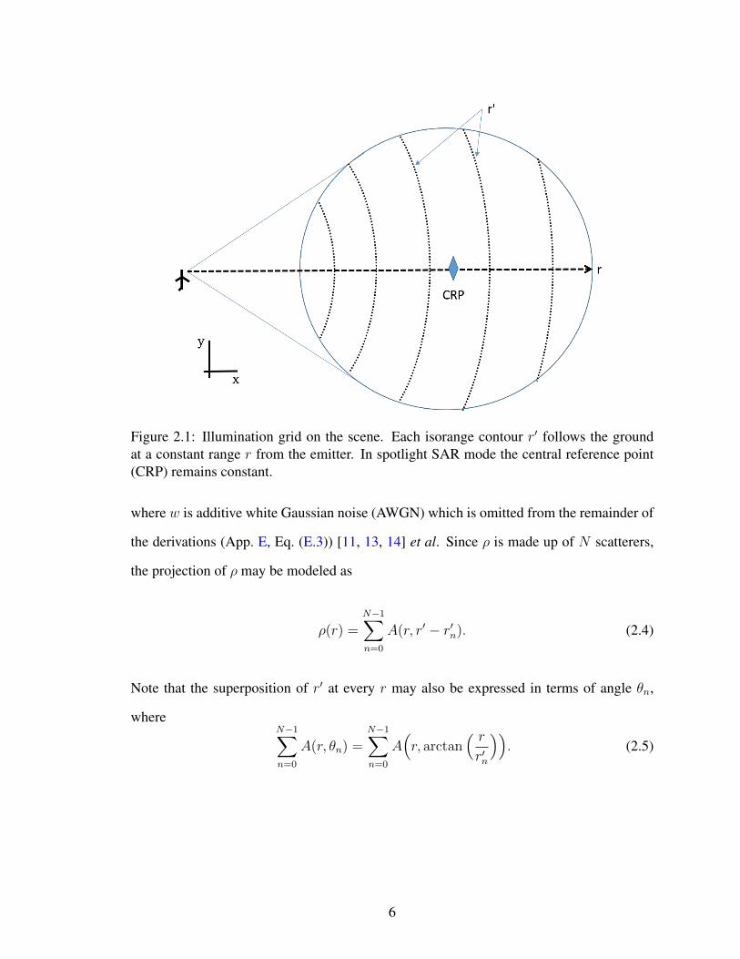
Figure 2.1: Illumination grid on the scene. Each isorange contour r′ follows the groundat a constant range r from the emitter. In spotlight SAR mode the central reference point(CRP) remains constant.
where w is additive white Gaussian noise (AWGN) which is omitted from the remainder of
the derivations (App. E, Eq. (E.3)) [11, 13, 14] et al. Since ρ is made up of N scatterers,
the projection of ρ may be modeled as
ρ(r) =N−1∑n=0
A(r, r′ − r′n). (2.4)
Note that the superposition of r′ at every r may also be expressed in terms of angle θn,
whereN−1∑n=0
A(r, θn) =N−1∑n=0
A(r, arctan
( rr′n
)). (2.5)
6
The time shifts τn and frequency shifts fdn for each scatterer are dependent on their location
(xn, yn) and velocity vn relative to the emitter through
τn =2√x2n + y2
n
c(2.6)
fdn =2vnfc cos(θn)
c=
2vnfc cos(
arctan(ynxn
))c
=2vfcyn
c√x2n + y2
n
, (2.7)
assuming xn 6= 0. Eqs. (2.4), (2.6), and (2.7) allow the forward model Eq. (2.3) to be
modeled in the more common form, for one pulse,
sRx(t) = A0
N−1∑n=0
p(t− τn)Anej2π(fc+fdn)(t−τn)+jπk(t−τn)2 , (2.8)
which shows the amplitude, time, and frequency shifts that represent the scene within the
forward model of a LFM signal.
2.2.1 Kinematic and Processing Model
The scene reflectivity density is embedded in the waveform through the time, Doppler,
and amplitude shifts of Eqns. (2.6) and (2.7), as shown in Eq. (2.8). However, Eqns (2.6)
and (2.7) are not limited to a position and velocity model. Throughout a CPI, the trans-
mitted waveform reflects from the scene at some time-varying distance defined by x and
y, while the platform is traveling at speed −→v with acceleration −→a . A notation that is more
commonly used in SAR signal models is
K(−→r ,−→v ,−→a ; t) =
−→r = xx(t) + yy(t) + zz(t)
−→v = xvx(t) + yvy(t) + zvz(t)
−→a = xax(t) + yay(t) + zaz(t),
(2.9)
7
Figure 2.2: General data processing model.
and could include modeling of roll, pitch, yaw, or other motions of the radar platform. A
high fidelity model may utilize even more detail, such as the level of detail afforded by the
Brawler and BLUEMAX models [28, 29].
An ideal K for traditional spotlight SAR results in polar-format data with uniform
sampling in frequency and angle, however errors induced by a non-ideal K (such as range
migration and antenna vibration) result in uneven sampling. Other polar coordinate and
waveform considerations are discussed in Appendices A, B, and [13, 14, 15, 16, 17, 23].
Following the collection of M pulse returns, exploitation of the amplitude, time, and
frequency shifts is performed through an image formation process (IFP). Although there
are numerous methods of processing spotlight SAR data into an image, they maintain the
common goal of forming a “clear” image, and generally follow the steps discussed next. As
shown in Fig. 2.2, the received signal is demodulated if necessary and then sampled by an
analog-to-digital converter, after which the IFP forms an image as a 2-D map. An IFP, such
as the down-sampled matched filter (DMF) or polar-format algorithm (PFA), is utilized to
focus the scene data. Due to space-variant and invariant errors that may occur during the
collection, some auto-focus technique may be applied to the image to focus the final image
ρ [16, 13]. A more in depth discussion of this processing model and the DMF is provided
in Appendix C and [13, 14, 15, 16, 18]. Also, an example case for the matched-filter and
deramp process of an LFM signal is provided in App. E.
Typical IFPs utilize demodulation techniques to isolate the time and Doppler shifts.
For example a spotlight SAR system that utilizes the traditional PFA to process a received
LFM waveform will result in an image which contains two well known sources of phase
8
error. Residual video phase will be present due to incomplete demodulation if only a de-
ramp procedure is utilized (App. E, Eq. (E.19)) [11, 13, 14] et al. Error due to range
curvature, which manifests as a quadratic phase change, will be present since the PFA’s
matched-filter is based on the first-order Taylor series of the differential range between the
radar and a reference range [35]2. Both errors may be corrected in order to isolate the
desired information in a form that results in a clear image [11, 13, 14, 35]. Regardless,
residual artifacts and methods to correct them, which are specific to the waveforms and/or
IFPs used, are well documented and expected to be utilized in order to produce a quality
image [11, 13, 14, 18] et al.
The IFP used to simulate the examples in this paper is a Taylor-windowed DMF (dis-
cussed in Appendix C, Eq. (C.2), and [19]). While this IFP is known to be slower than
some other IFPs, the DMF’s matched filter is calculated from the full forward model to
include range-curvature. The simulated radar’s K is limited to
−→r (t) = ~r0 + ~vt (2.10)
−→r0 = xx0 + yy0 + zz0 (2.11)
~v = yv0 (2.12)
where x0 and y0 are the initial range and cross-range to the CRP, and v0 is the initial ve-
locity of the emitter platform. The radar’s waveform parameters are provided in Table 2.1,
where fc, BW, PW, k, and PRI are the carrier frequency, bandwidth, pulse width, linear-
frequency modulation rate, and pulse repetition interval, respectively3. Figure 2.3 provides
an example result of this IFP for a bed-of-nails scene. The examples provided in this paper
are limited to individual point scatterers for convenience and to allow objective compar-
2Range curvature error will be noticeable if the scene extent is large enough, as detailed in [35].3Although the PW used is unrealistic (3-60 µs is more common [18]), it is used throughout the examples
in order to show blurring effects clearly.
9
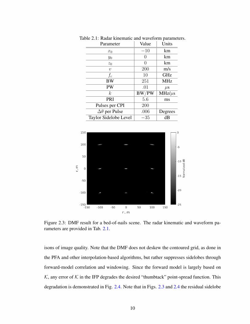
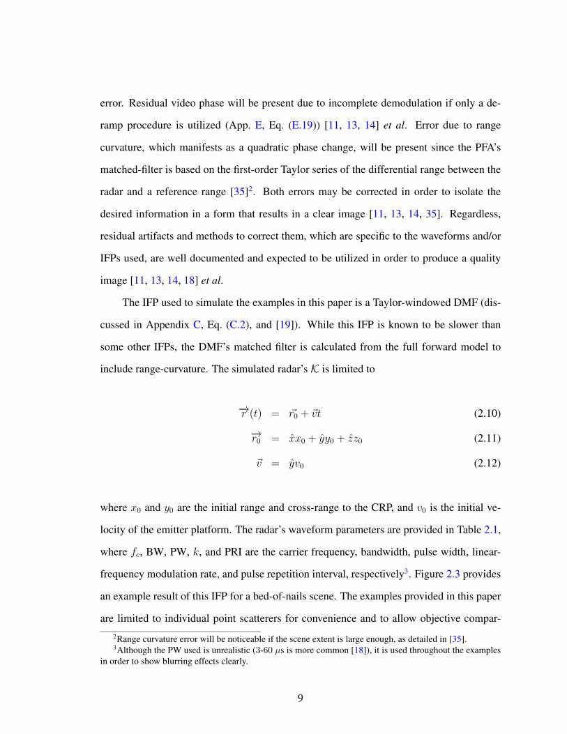
Table 2.1: Radar kinematic and waveform parameters.Parameter Value Units
x0 −10 kmy0 0 kmz0 0 kmv 200 m/sfc 10 GHz
BW 251 MHzPW .01 µsk BW/PW MHz/µs
PRI 5.6 msPulses per CPI 200∆θ per Pulse .006 Degrees
Taylor Sidelobe Level −35 dB
Figure 2.3: DMF result for a bed-of-nails scene. The radar kinematic and waveform pa-rameters are provided in Tab. 2.1.
isons of image quality. Note that the DMF does not deskew the contoured grid, as done in
the PFA and other interpolation-based algorithms, but rather suppresses sidelobes through
forward-model correlation and windowing. Since the forward model is largely based on
K, any error of K in the IFP degrades the desired “thumbtack” point-spread function. This
degradation is demonstrated in Fig. 2.4. Note that in Figs. 2.3 and 2.4 the residual sidelobe
10
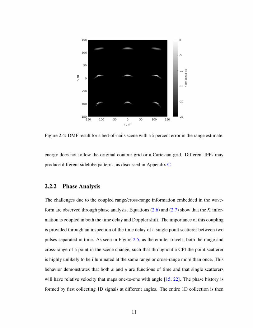
Figure 2.4: DMF result for a bed-of-nails scene with a 5 percent error in the range estimate.
energy does not follow the original contour grid or a Cartesian grid. Different IFPs may
produce different sidelobe patterns, as discussed in Appendix C.
2.2.2 Phase Analysis
The challenges due to the coupled range/cross-range information embedded in the wave-
form are observed through phase analysis. Equations (2.6) and (2.7) show that the K infor-
mation is coupled in both the time delay and Doppler shift. The importance of this coupling
is provided through an inspection of the time delay of a single point scatterer between two
pulses separated in time. As seen in Figure 2.5, as the emitter travels, both the range and
cross-range of a point in the scene change, such that throughout a CPI the point scatterer
is highly unlikely to be illuminated at the same range or cross-range more than once. This
behavior demonstrates that both x and y are functions of time and that single scatterers
will have relative velocity that maps one-to-one with angle [15, 22]. The phase history is
formed by first collecting 1D signals at different angles. The entire 1D collection is then
11
Figure 2.5: The change in range and cross-range contours for two different points of aflight path. With a pulse transmitted at each angle, the target resides on different range andcross-range contours, resulting in a change in phase.
mapped into a 2D fast-time tf , slow-time ts array, where for M pulses
ts ∈ (0,MPRI) (2.13)
∆ts = PRI (2.14)
tf ∈ (0,PRI) (2.15)
∆tf =PW
TBW, (2.16)
where the time-bandwidth product TBW is a measure of pulse compression [11, 12]. An
example of the phase argument response from a single scatterer throughout a synthetic
aperture is provided in Fig. 2.6 which demonstrates that the phase arguments provide a
12
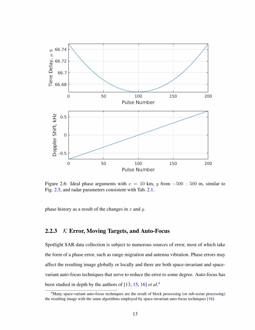
Figure 2.6: Ideal phase arguments with x = 10 km, y from −500 : 500 m, similar toFig. 2.5, and radar parameters consistent with Tab. 2.1.
phase history as a result of the changes in x and y.
2.2.3 K Error, Moving Targets, and Auto-Focus
Spotlight SAR data collection is subject to numerous sources of error, most of which take
the form of a phase error, such as range migration and antenna vibration. Phase errors may
affect the resulting image globally or locally and there are both space-invariant and space-
variant auto-focus techniques that serve to reduce the error to some degree. Auto-focus has
been studied in depth by the authors of [13, 15, 16] et al.4
4Many space-variant auto-focus techniques are the result of block processing (or sub-scene processing)the resulting image with the same algorithms employed by space-invariant auto-focus techniques [16].
13
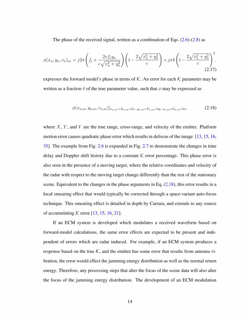
The phase of the received signal, written as a combination of Eqs. (2.6)-(2.8) as
φ(xn, yn, vn)m = j2π
(fc +
2vfcyn
c√x2n + y2
n
)(t−
2√x2n + y2
n
c
)+ jπk
(t−
2√x2n + y2
n
c
)2
,
(2.17)
expresses the forward model’s phase in terms of K. An error for each K parameter may be
written as a fraction δ of the true parameter value, such that φ may be expressed as
φ(xn,m, yn,m, vn,m)|xn,m=Xn,m+δx, yn,m=Yn,m+δy, vn,m=Vn,m+δv, (2.18)
where X , Y , and V are the true range, cross-range, and velocity of the emitter. Platform
motion error causes quadratic phase error which results in defocus of the image [13, 15, 16,
35]. The example from Fig. 2.6 is expanded in Fig. 2.7 to demonstrate the changes in time
delay and Doppler shift history due to a constant K error percentage. This phase error is
also seen in the presence of a moving target, where the relative coordinates and velocity of
the radar with respect to the moving target change differently than the rest of the stationary
scene. Equivalent to the changes in the phase arguments in Eq. (2.18), this error results in a
local smearing effect that would typically be corrected through a space-variant auto-focus
technique. This smearing effect is detailed in depth by Carrara, and extends to any source
of accumulating K error [13, 15, 16, 21].
If an ECM system is developed which modulates a received waveform based on
forward-model calculations, the same error effects are expected to be present and inde-
pendent of errors which are radar induced. For example, if an ECM system produces a
response based on the true K, and the emitter has some error that results from antenna vi-
bration, the error would effect the jamming energy distribution as well as the normal return
energy. Therefore, any processing steps that alter the focus of the scene data will also alter
the focus of the jamming energy distribution. The development of an ECM modulation
14
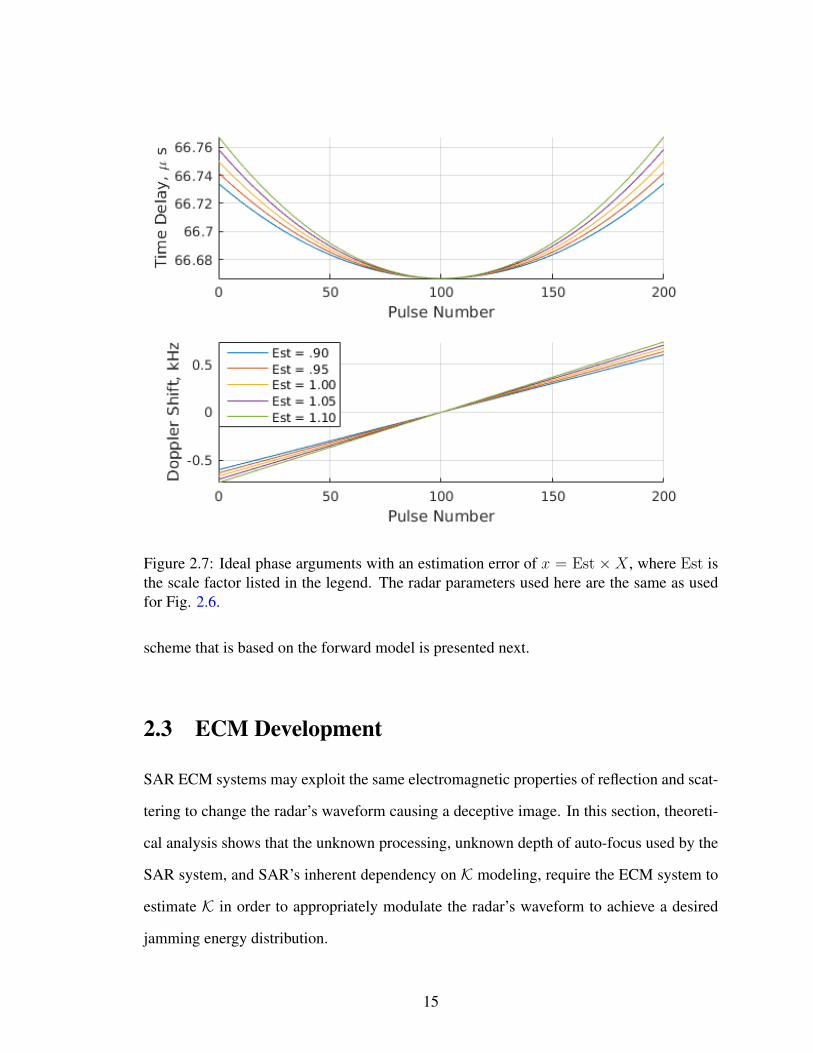
Figure 2.7: Ideal phase arguments with an estimation error of x = Est ×X , where Est isthe scale factor listed in the legend. The radar parameters used here are the same as usedfor Fig. 2.6.
scheme that is based on the forward model is presented next.
2.3 ECM Development
SAR ECM systems may exploit the same electromagnetic properties of reflection and scat-
tering to change the radar’s waveform causing a deceptive image. In this section, theoreti-
cal analysis shows that the unknown processing, unknown depth of auto-focus used by the
SAR system, and SAR’s inherent dependency on K modeling, require the ECM system to
estimate K in order to appropriately modulate the radar’s waveform to achieve a desired
jamming energy distribution.
15

An ECM system may receive a signal from the emitter, modify it, and transmit it back
to the emitter in order to embed false information in the waveform. As previously stated, the
jammer is assumed to have basic DRFM capabilities, such as those detailed by the authors
of [1]. With the appropriate waveform modification this may result in the formation of a
desired energy distribution in the final image. Additive jamming energy J augments the
received signal as
sRx(t) = sRx
(ρ(t), sTx(t),K(t)
)+ sRx
(ρJ(t), sTx(t),KJ(t)
), (2.19)
where ρJ represents the scene density that the ECM signal embeds and KJ is the jammer’s
estimate of K.
The DRFM applies the amplitude, time, and frequency shifts to the waveform in dif-
ferent ways. First, the amplitude is likely to be held at a maximum in order to maintain
the highest possible jamming-to-signal ratio. The time shift is accomplished through de-
laying the transmission of the recorded pulse for an appropriate amount of time. If the
ECM system is capable of estimating the radar’s PRI then the target may also be effec-
tively placed in front of the jammer in range [1, 2, 3]. The frequency shift may be applied
through multiplication of the recorded signal with a designed coefficient or set of coeffi-
cients [2, 3, 26, 27].
An approach to ECM waveform development begins with the generation of a single
false target at a desired point in the reconstructed image. As seen in Fig. 2.8, from the
jammer’s perspective at location (xJ , yJ ) a received pulse has a specific angle of arrival
and therefore requires different modulation coefficients in order to produce a false target
displaced by some ∆x1 and ∆y1 from the jammer. Assuming the radar position is xr =
16
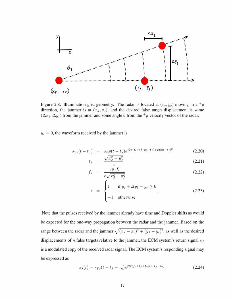
Figure 2.8: Illumination grid geometry. The radar is located at (xr, yr) moving in a +ydirection, the jammer is at (xJ , yJ ), and the desired false target displacement is some(∆x1,∆y1) from the jammer and some angle θ from the +y velocity vector of the radar.
yr = 0, the waveform received by the jammer is
sTx(t− tJ) = A0p(t− tJ)ej2π(fc+εfJ )(t−tJ )+jπk(t−tJ )2 (2.20)
tJ =
√x2J + y2
J
c(2.21)
fJ =vyJfc
c√x2J + y2
J
(2.22)
ε =
1 if yj + ∆y1 − yr ≥ 0
−1 otherwise. (2.23)
Note that the pulses received by the jammer already have time and Doppler shifts as would
be expected for the one-way propagation between the radar and the jammer. Based on the
range between the radar and the jammer√
(xJ − xr)2 + (yJ − yr)2, as well as the desired
displacements of n false targets relative to the jammer, the ECM system’s return signal sJ
is a modulated copy of the received radar signal. The ECM system’s responding signal may
be expressed as
sJ(t) = sTx(t− tJ − τn)ej2π(fc+fJ+fn)(t−tJ−τn), (2.24)
17
where theK based time shift (Eq. (2.6)) and Doppler shift (Eq. (2.7)) are calculated through
x1 = xJ − xr + ∆x1 (2.25)
y1 = yJ − yr + ∆y1 (2.26)
v1 = vr + ∆v (2.27)
τn = 2
(√x2
1 + y21
c− tj
)(2.28)
fn = 2
(v1y1fc
c√x2
1 + y21
− fJ
)(2.29)
to embed theK-based false target facsimile into the ECM’s waveform. Note that Eqs. (2.28)
and (2.29) are both offset by one propagation factor relative to the jammer, tj and fj , in
order to ensures that once the waveform propagates from the jammer to the receiver the
time delay and Doppler shift specific to the jammer will no longer be in the waveform.
To demonstrate, assume the jammer received an LFM waveform modeled by Eq. (2.20).
Following Eq. (2.24), the modulated signal transmitted by the jammer is
sJ(t) = p(t− tJ)e−j2π(fc+fJ )(t−tJ )−jπk(t−tJ )2)
× p(t− τn)e−j2πfnt (2.30)
= p
(t− 2
√x2
1 + y21
c+ tJ
)e−jΦ (2.31)
Φ = 2π
(fc +
2v1y1fc
c√x2
1 + y21
− vyJfc
c√x2J + y2
J
)(t− 2
√x2
1 + y21
c+ tJ
)
− πk
(t− 2
√x2
1 + y21
c+ tJ
)2
,
(2.32)
18
such that the forward model at the face of the receiver becomes
sRx = p
(t− 2
√x2
1 + y21
c
)e−jΦ (2.33)
Φ = 2π
(fc +
2v1y1fc
c√x2
1 + y21
)(t− 2
√x2
1 + y21
c
)
− πk
(t− 2
√x2
1 + y21
c
)2
, (2.34)
as would be expected from the pulse return of a scatterer at the false target’s location.
A numerical example is provided with the following radar, ECM, and false target
location (xF , yF ) and displacement in meters:
xr, yr = (0, 0) (2.35)
xJ , yJ = (400, 300) (2.36)
xF , yF = (500, 1200) (2.37)
∆x1,∆y1 = (100, 900), (2.38)
as shown in Fig. 2.8. The radar emits a pulse which propagates to the ECM location. The
signal model changes according to Eq. (2.20) at the ECM’s reception of the pulse such that
tJ =500
c(2.39)
fJ =vrfcc
300
500. (2.40)
The ECM system delays and modulates the received signal according to Eqs. (2.28) and (2.29)
19
such that
τn =1300− 500
c(2.41)
fn =vrfcc
(1200
1300− 300
500
). (2.42)
The one-way propagation from the jammer back to the radar results in the forward model
expressed in Eq. (2.34) with the following time and Doppler shifts
τn =2(1300)
c=
2√
5002 + 12002
c(2.43)
fn =2vrfcc
(1200
1300
), (2.44)
as would be expected from the pulse return of a scatterer at the false target’s location.
2.4 Summary
Equation (2.24) provides the K-based modulation which an ECM system may implement
in order to ensure the desired jamming energy distribution forms in the final image. Where
there are multiple ways for an ECM system to estimate the SAR platform’s K, the level
of precision required to maintain confidence in the resultant jamming energy distribution
quality may be found through modeling and simulation.
20
Methodology
3.1 Proposed Study
To support the hypothesis that the quality of the resulting jamming energy distribution is
limited by the accuracy of the forward-model based ECM system’s estimation of the radar’s
K, the sensitivity of jamming energy distributions to K error is assessed through Monte
Carlo simulation. These simulations have a defined accuracy as discussed in Sec. 3.2.2.
Since the K variables x1, y1, and v1, defined by Eqs. (2.25), (2.26), and (2.27), do
not contribute to the phase equivalently, they are evaluated individually to observe any
characteristics that are unique to each parameter. Three sets of Monte Carlo simulations
are performed, each with one K variable treated as a uniform random variable and the
other two as constants. For each Monte Carlo set the random variable is given a standard
deviation σ, individually denoted as σxr , σyr , and σvr . Following signal modeling and
DMF processing, the Jaccard Distance is used to quantify the final image’s similarity with
an ideal image, discussed further in Sec. 3.2.3. The ideal image is generated through a zero-
error K calculation and a noiseless system. Note that the exact source of the K-estimation
error is not of interest here.
Since any jamming distribution may be made through the use of a sufficient number of
false point targets, the degradation of a single false target located at the CRP is evaluated.
The results are presented in 2D graphs that compare each standard deviation of one K
parameter and the average Monte Carlo result of the Jaccard Distance to allow one to
21

form a conclusion of how sensitive the jamming energy distribution is to K error within a
specified confidence level.
3.2 Experiment Procedure
The combination of the emitter models, Monte Carlo accuracy derivation, and Jaccard dis-
tance metric, discussed next, provide the tools required to assess the sensitivity of an ECM
system’s control of the jamming energy distribution to K errors. The following steps are
proposed:
1. Generate the reference image; an ideal and noiseless SAR image based on Tabs. 3.1
and 3.2.
2. Demonstrate the average Jaccard distance for a−20 to 20 signal-to-noise ratio sweep.
3. For each standard deviation σxr , σyr , and σvr , empirically find the equivalent Jaccard
distance standard deviation σ. This step and those that follow are noiseless. The
standard deviations for σxr and σyr range between [10−3, 102] m with a logarithmic
step size. The standard deviations for σvr range between [10−3, 102] m/s with a
logarithmic step size.
4. Estimate the necessary number of Monte Carlo trials N for each σ, found in step 2,
through Eq. (3.6) with the confidence coefficient zc that corresponds to the confidence
level of 98%. These steps provide that with 98% confidence the estimated Jaccard
distance for each specific σ is accurate to within 4 % of the true average. The values
of 98% and 4% were arbitrarily chosen.
5. Run the Monte Carlo trials for eachN corresponding to the appropriate σ. MATLAB R©’s
rand function is used to calculate the appropriate population samples (Sec. 3.2.2) [34].
22
6. Display the trends of each σ versus the average Jaccard distance and discuss any key
characteristics of the results.
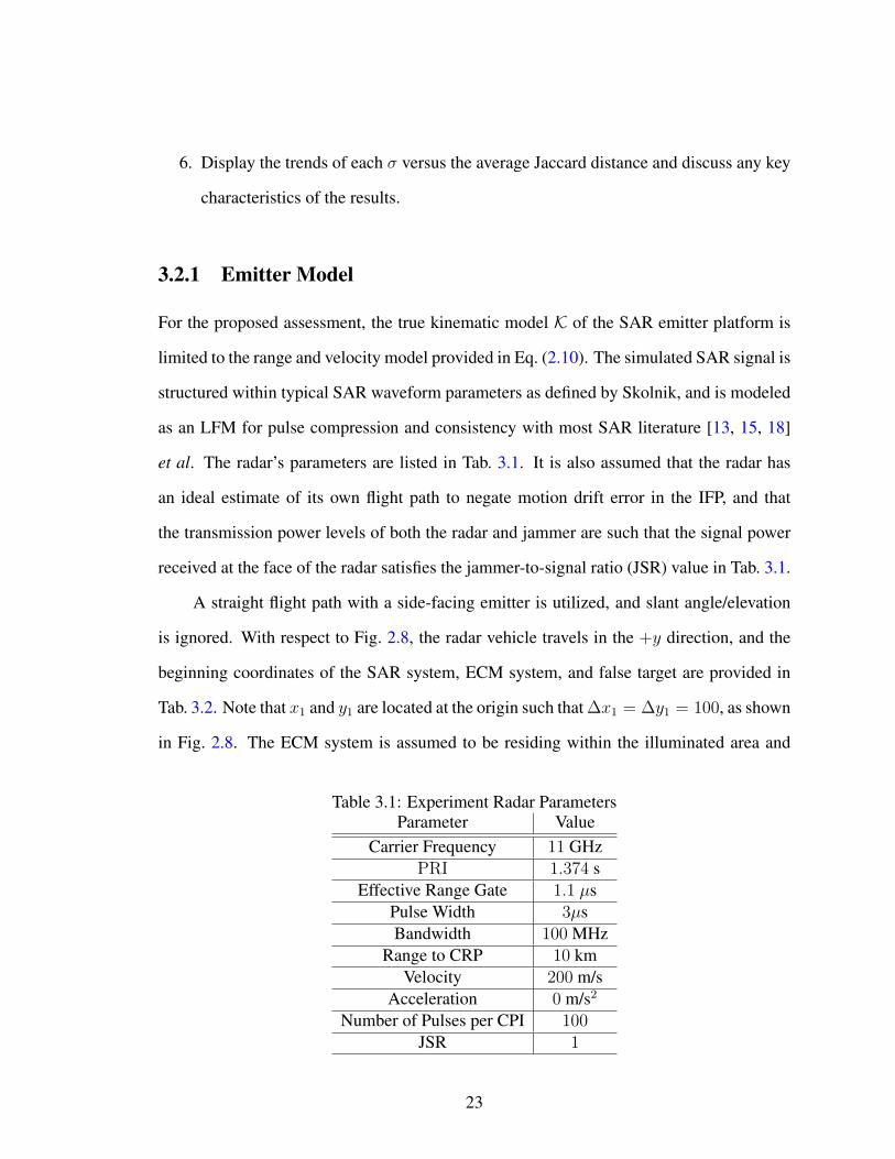
3.2.1 Emitter Model
For the proposed assessment, the true kinematic model K of the SAR emitter platform is
limited to the range and velocity model provided in Eq. (2.10). The simulated SAR signal is
structured within typical SAR waveform parameters as defined by Skolnik, and is modeled
as an LFM for pulse compression and consistency with most SAR literature [13, 15, 18]
et al. The radar’s parameters are listed in Tab. 3.1. It is also assumed that the radar has
an ideal estimate of its own flight path to negate motion drift error in the IFP, and that
the transmission power levels of both the radar and jammer are such that the signal power
received at the face of the radar satisfies the jammer-to-signal ratio (JSR) value in Tab. 3.1.
A straight flight path with a side-facing emitter is utilized, and slant angle/elevation
is ignored. With respect to Fig. 2.8, the radar vehicle travels in the +y direction, and the
beginning coordinates of the SAR system, ECM system, and false target are provided in
Tab. 3.2. Note that x1 and y1 are located at the origin such that ∆x1 = ∆y1 = 100, as shown
in Fig. 2.8. The ECM system is assumed to be residing within the illuminated area and
Table 3.1: Experiment Radar ParametersParameter Value
Carrier Frequency 11 GHzPRI 1.374 s
Effective Range Gate 1.1 µsPulse Width 3µsBandwidth 100 MHz
Range to CRP 10 kmVelocity 200 m/s
Acceleration 0 m/s2
Number of Pulses per CPI 100JSR 1
23
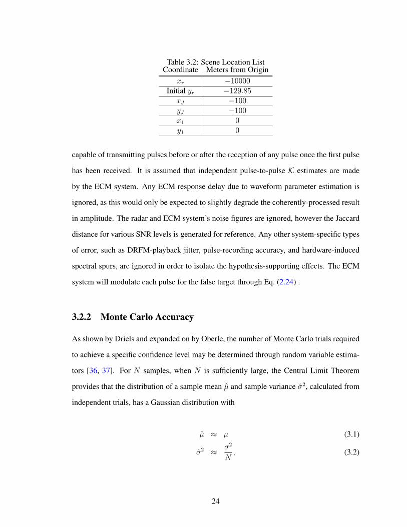
Table 3.2: Scene Location ListCoordinate Meters from Origin
xr −10000Initial yr −129.85xJ −100yJ −100x1 0y1 0
capable of transmitting pulses before or after the reception of any pulse once the first pulse
has been received. It is assumed that independent pulse-to-pulse K estimates are made
by the ECM system. Any ECM response delay due to waveform parameter estimation is
ignored, as this would only be expected to slightly degrade the coherently-processed result
in amplitude. The radar and ECM system’s noise figures are ignored, however the Jaccard
distance for various SNR levels is generated for reference. Any other system-specific types
of error, such as DRFM-playback jitter, pulse-recording accuracy, and hardware-induced
spectral spurs, are ignored in order to isolate the hypothesis-supporting effects. The ECM
system will modulate each pulse for the false target through Eq. (2.24) .
3.2.2 Monte Carlo Accuracy
As shown by Driels and expanded on by Oberle, the number of Monte Carlo trials required
to achieve a specific confidence level may be determined through random variable estima-
tors [36, 37]. For N samples, when N is sufficiently large, the Central Limit Theorem
provides that the distribution of a sample mean µ and sample variance σ2, calculated from
independent trials, has a Gaussian distribution with
µ ≈ µ (3.1)
σ2 ≈ σ2
N, (3.2)
24
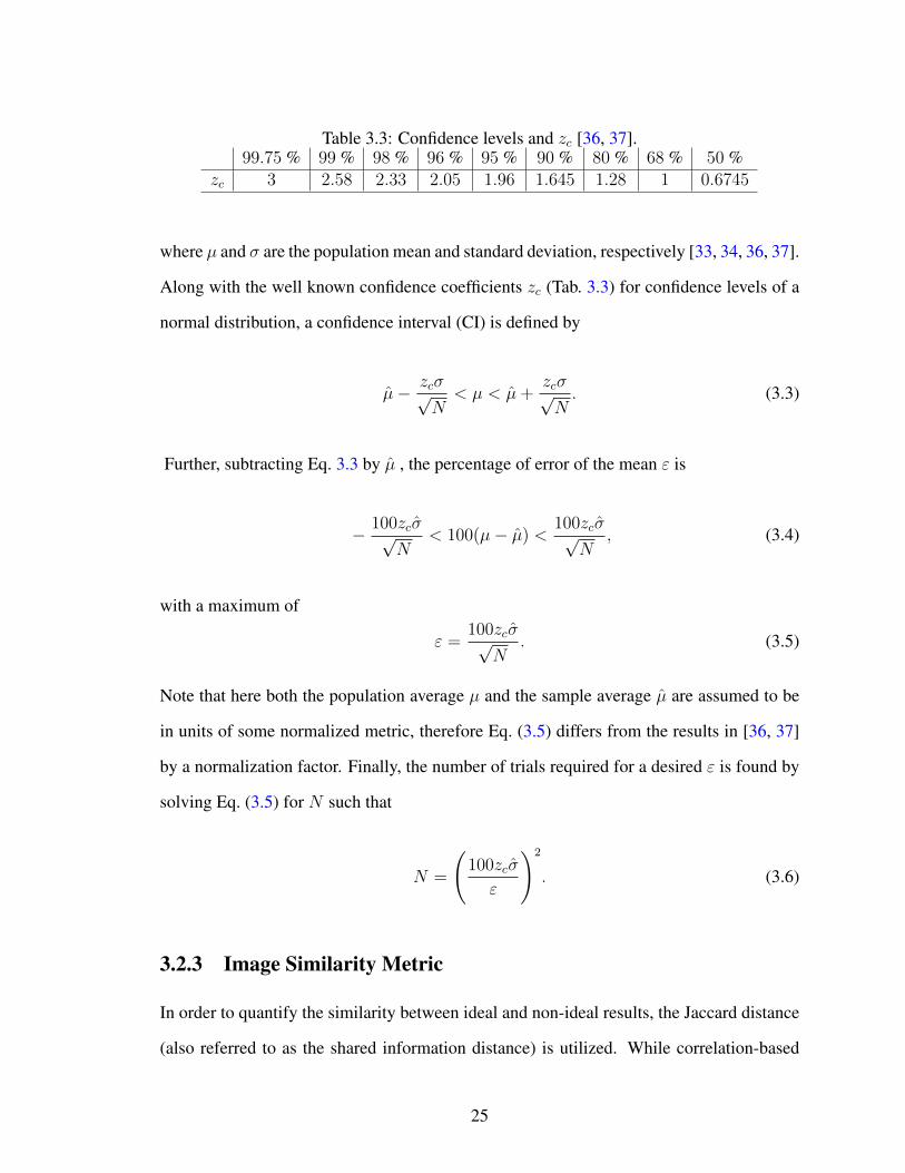
Table 3.3: Confidence levels and zc [36, 37].99.75 % 99 % 98 % 96 % 95 % 90 % 80 % 68 % 50 %
zc 3 2.58 2.33 2.05 1.96 1.645 1.28 1 0.6745
where µ and σ are the population mean and standard deviation, respectively [33, 34, 36, 37].
Along with the well known confidence coefficients zc (Tab. 3.3) for confidence levels of a
normal distribution, a confidence interval (CI) is defined by
µ− zcσ√N< µ < µ+
zcσ√N. (3.3)
Further, subtracting Eq. 3.3 by µ , the percentage of error of the mean ε is
− 100zcσ√N
< 100(µ− µ) <100zcσ√
N, (3.4)
with a maximum of
ε =100zcσ√
N. (3.5)
Note that here both the population average µ and the sample average µ are assumed to be
in units of some normalized metric, therefore Eq. (3.5) differs from the results in [36, 37]
by a normalization factor. Finally, the number of trials required for a desired ε is found by
solving Eq. (3.5) for N such that
N =
(100zcσ
ε
)2
. (3.6)
3.2.3 Image Similarity Metric
In order to quantify the similarity between ideal and non-ideal results, the Jaccard distance
(also referred to as the shared information distance) is utilized. While correlation-based
25

measurements are valid, they are more sensitive to translational changes in the image due to
their nature as a measurement of linear dependency between two objects than entropy-based
methods. Euclidean distance and other Minkowski distances are spatially dependent and
therefore also more sensitive to translational shifts than entropy-based methods. Therefore,
an entropy-based measurement was chosen due to its increased sensitivity to structural
changes in the compared images [32].
The authors of [31, 32] demonstrate that many entropy based measures used in the
past to compare image similarity do not satisfy the fundamental requirements for a dis-
tance metric, commonly known as the identity axiom, the triangle inequality, the symmetry
axiom, and that a distance is always positive (App. D). However, they provide the following
definition of the Jaccard distance which does satisfy these requirements:
d(A,B) = HAB −MI, (3.7)
whereHAB is the joint entropy of imagesA andB, andMI is their mutual information [32,
33]. Since “image similarity” is not an easily perceived distance, the Jaccard Distance is
more clearly understood (and less subjective) when normalized such that
D(A,B) =d(A,B)
HAB
∈ [0, 1], (3.8)
where a value of zero denotes when A and B are the most similar, and a value of one
denotes when A and B are the most dissimilar. Translational, rotational, and noise affects
on the Jaccard Distance are demonstrated in App. D.
Note that while the Jaccard distance is being used for image similarity measurements,
the images themselves represent cross-ambiguity functions of the transmitted signal and
the scene, as expressed in Eq. (2.3). Small shifts in the scene may cause the sidelobes to
act constructively or destructively, so it is possible for a small shift in the K estimate to
26

cause an increase or decrease in the Jaccard distance. However, as the K error continues to
increase, a generally increasing (furthering) trend is expected in the Jaccard distance.
27
Results
Following step 1, as defined in Sec. 3.2, the ideal reference image was formed from the
geometry shown in Fig. 4.1a, as described by the parameters given in Tabs. 2.1 and 3.2.
The ideal range history for both the ECM location and the false target location is shown
in Fig. 4.1b. The generated comparison image is shown in Fig. 4.2. Following step 2, as
defined in Sec. 3.2, the average Jaccard distance for various SNR values is demonstrated in
Fig. 4.3.
Following steps 3 and 4, the standard deviation of the Jaccard σ for each K parameter
was directly calculated at σx, σy, and σv. These values were used to calculate the required
number of trials N . The resulting N trials required to achieve a 98% confidence level
that the Monte Carlo results for each step in standard deviation are with in 4% of the true
average is shown in Fig. 4.4.
28
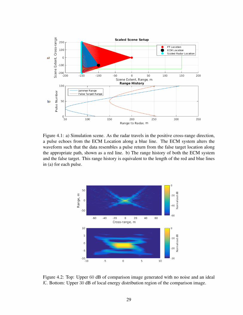
Figure 4.1: a) Simulation scene. As the radar travels in the positive cross-range direction,a pulse echoes from the ECM Location along a blue line. The ECM system alters thewaveform such that the data resembles a pulse return from the false target location alongthe appropriate path, shown as a red line. b) The range history of both the ECM systemand the false target. This range history is equivalent to the length of the red and blue linesin (a) for each pulse.
Figure 4.2: Top: Upper 60 dB of comparison image generated with no noise and an idealK. Bottom: Upper 30 dB of local energy distribution region of the comparison image.
29
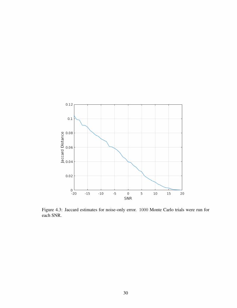
Figure 4.3: Jaccard estimates for noise-only error. 1000 Monte Carlo trials were run foreach SNR.
30
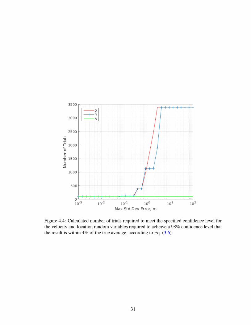
Figure 4.4: Calculated number of trials required to meet the specified confidence level forthe velocity and location random variables required to acheive a 98% confidence level thatthe result is within 4% of the true average, according to Eq. (3.6).
31
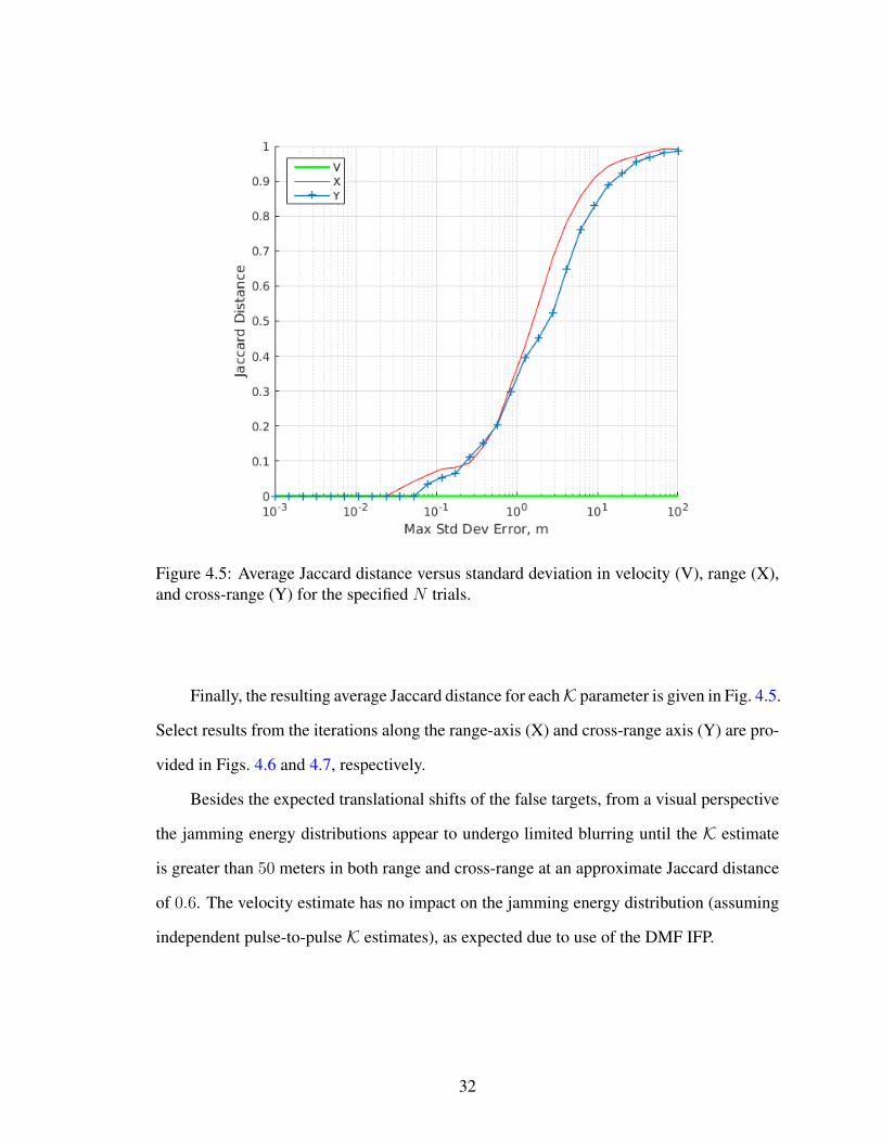
Figure 4.5: Average Jaccard distance versus standard deviation in velocity (V), range (X),and cross-range (Y) for the specified N trials.
Finally, the resulting average Jaccard distance for eachK parameter is given in Fig. 4.5.
Select results from the iterations along the range-axis (X) and cross-range axis (Y) are pro-
vided in Figs. 4.6 and 4.7, respectively.
Besides the expected translational shifts of the false targets, from a visual perspective
the jamming energy distributions appear to undergo limited blurring until the K estimate
is greater than 50 meters in both range and cross-range at an approximate Jaccard distance
of 0.6. The velocity estimate has no impact on the jamming energy distribution (assuming
independent pulse-to-pulse K estimates), as expected due to use of the DMF IFP.
32

4.1 Use Case Example
While the results shown are unique to the DMF IFP and an LFM waveform, they demon-
strate the usefulness of the assessment method. Any other waveform or IFP will have
similar but unique results which may be assessed through the same method. Further con-
straining the Jaccard calculation to a minimum desired dB from the peak of the mainlobe
and isolating a region of interest (likely the mainlobe, regardless of translation) would im-
prove the intuition afforded by the results. Also, evaluating the point spread function at
every individual pixel would allow for the development of Jaccard contour maps, which
would be valuable since the change in the jamming energy distribution is not likely sym-
metric about any axis. The Jaccard contour maps for all 3 K parameter pairs, (x,y), (x,v),
and (y,v), may assist in identifying ECM system regions of operability.
33
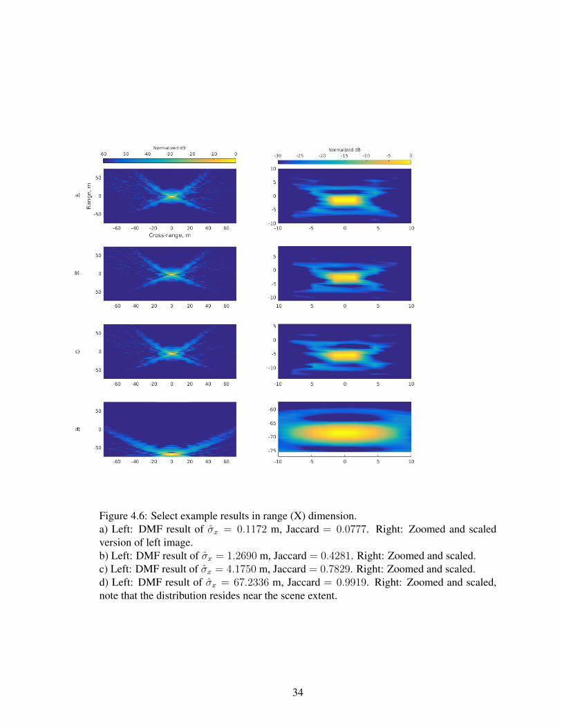
Figure 4.6: Select example results in range (X) dimension.a) Left: DMF result of σx = 0.1172 m, Jaccard = 0.0777. Right: Zoomed and scaledversion of left image.b) Left: DMF result of σx = 1.2690 m, Jaccard = 0.4281. Right: Zoomed and scaled.c) Left: DMF result of σx = 4.1750 m, Jaccard = 0.7829. Right: Zoomed and scaled.d) Left: DMF result of σx = 67.2336 m, Jaccard = 0.9919. Right: Zoomed and scaled,note that the distribution resides near the scene extent.
34
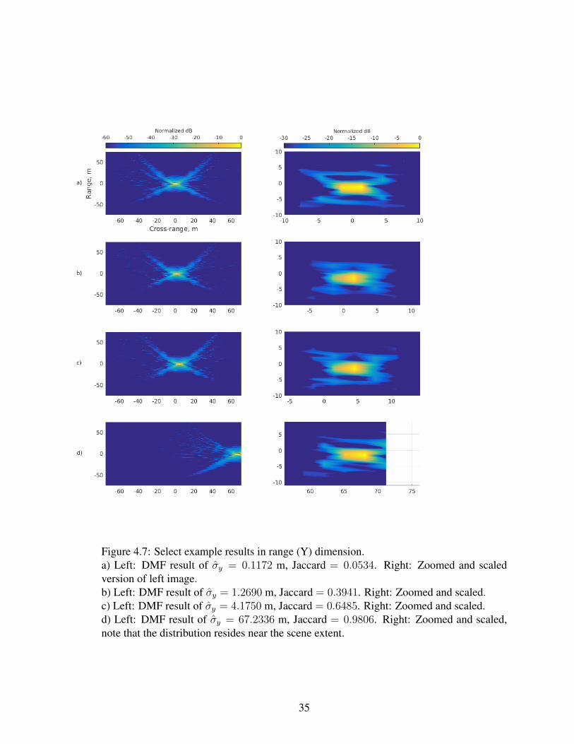
Figure 4.7: Select example results in range (Y) dimension.a) Left: DMF result of σy = 0.1172 m, Jaccard = 0.0534. Right: Zoomed and scaledversion of left image.b) Left: DMF result of σy = 1.2690 m, Jaccard = 0.3941. Right: Zoomed and scaled.c) Left: DMF result of σy = 4.1750 m, Jaccard = 0.6485. Right: Zoomed and scaled.d) Left: DMF result of σy = 67.2336 m, Jaccard = 0.9806. Right: Zoomed and scaled,note that the distribution resides near the scene extent.
35
Conclusion
Throughout this thesis it has been shown that the quality of the resulting jamming energy
distribution is clearly limited to the ECM system’s K estimate accuracy. The modeling
of the LFM forward model allowed for the development of the forward-model based false-
target ECM method. The appropriately constrained Jaccard distance allowed for the change
in jamming energy distributions to be measured. The Central Limit Theorem and Law
of Large Numbers allowed for the Jaccard distance calculations to be bounded within a
specified level of accuracy. Further, the assessment method was extended to a practical
use-case example.
In general, this thesis has provided that an ECM system designer may assess the worst-
case K estimation as a limit to the accuracy and quality of jamming energy distribution
formation. Future work may include an extension to moving target indicators, optimum
scene design with regards to resolvability, development of Jaccard contour maps, and the
development of a tracking-jamming combined system.
36
Bibliography
[1] T. Kusel, M. Inggs, J. Pienaar, “A Comparison Between The Spectral Fidelity of
Three Digital Radio Frequency Memory Architectures,” in Transactions of the AOC,
2004.
[2] D. Adamy, EW 101: A First Course in Electronic Warfare, Norwood, MA: Artech
House, Inc., 2001.
[3] P. J. Hannen, Radar and Electronic Warfare Principles for the Non-Specialist, 4th ed
Raleigh, NC: SciTech Publishing, 2013.
[4] R. S. Harness and M. C. Budge, Jr., “A Study on SAR Noise Jamming and False
Target Insertion,” in IEEE Southeast Conference, 2014.
[5] J. Jiang, Y. Wu, and H. Wang, “Analysis of Active Noise Jamming Against Synthetic
Aperture Radar Ground Moving Target Indication,” in 8th International Congress on
Image and Signal Processing, 2015.
[6] Y. Liu, T. Li, and Z. Gu, “Research on SAR Active Deception Jamming Generation
Technique,” in Fifth International Conference on Instrumentation and Measurement,
Computer, Communication and Control, 2015.
37
[7] M. Guo, N. Tai, H. Zhu, C. Wang, and N. Yuan, “Study on Inverse Synthetic Aperture
Radar Jamming Method Based on Sinusoidal Phase Modulations,” in IEEE Informa-
tion Technology, Networking, Electronic and Automation Control Conference, 2016.
[8] Q. Sun, T. Shu, S. Zhou, B. Tang, and W. Yu, “A Novel Jamming Signal Generation
Method for Deceptive SAR Jammer,” in IEEE Radar Conference, 2014.
[9] L. Xu, D. Feng, and X. Wang, “Improved Synthetic Aperture Radar Micro-Doppler
Jamming Method Based on Phase-Switched Screen,” IET Radar, Sonar, and Naviga-
tion, vol. 10, no. 3, 2016.
[10] B. Donnell, “Using Shadows to Detect Targets in Synthetic Aperture Radar Imagery,”
M.S. thesis, Dept. Eng., AFIT, Wright-Patterson Air Force Base, OH, 2009.
[11] R. E. Blahut, Theory of Remote Image Formation, 1st ed. The Edinburgh Building,
Cambridge CB2 2RU, UK: Cambridge University Press, 2004.
[12] N. Levanon, E. Mozeson Radar Signals Hoboken, NJ: John Wiley and Sons, Inc.,
2004.
[13] C. V. Jakowatz Jr, D. E. Wahl, P. H. Eichel, D. C. Ghiglia, P. A. Thompson, Spotlight-
Mode Synthetic Aperture Radar: A Signal Processing Approach Massachusetts:
Kluwer Academic Publishers, 1996.
[14] M. A. Richards, Fundamentals of Radar Signal Processing New York: McGraw-
Hill, 2005.
[15] J. C. Curlander, R. N. McDonough, Synthetic Aperture Radar Systems and Signal
Processing New York: John Wiley and Sons, Inc., 1991.
[16] W. G. Carrara, R. S. Goodman, R. M. Majewski, Spotlight Synthetic Aperture Radar
Signal Processing Algorithms Norwood, MA: Artech House, Inc., 1995.
38
[17] M. A. Richards, J. A. Scheer, W. A. Holm, Principles of Modern Radar Raleigh,
NC: SciTech Publishing, 2010.
[18] M. I. Skolnik, RADAR Handbook, 3rd ed. New York: McGraw-Hill, 2008.
[19] B. Edde, Radar: Principles, Technology, Applications Upper Saddle River, NJ:
Prentice Hall, PTR., 1995.
[20] K. E. Dungan, L. A. Gorham, L. J. Moore, “SAR Digital Spotlight Implementation in
MATLAB R©,” Proceedings of SPIE, vol. 8746, no. 87460A-1, 2013.
[21] Y. Liu, W. Wang, X. Pan, L. Xu, G. Wang, “Influence of Estimate Error of Radar
kinematic Parameter on Deceptive Jamming Against SAR,” IEEE Sensors Journal,
vol. 16, no. 15, 2016.
[22] C. A. Wiley, “Synthetic Aperture Radars: A Paradigm For Technology Evolution,”
IEEE Transactions on Aerospace and Electronic Systems, vol. AES-21, no. 2, 1985.
[23] G. W. Stimson, Introduction to Airborne Radar Raleigh, NC: SciTech Publishing,
1998.
[24] D. C. Munson, “Image Reconstruction from Frequency-Offset Fourier Data,“ Pro-
ceedings of the IEEE, vol. 72, no. 6, 1984.
[25] M. C. Budge, R. S. Harness, “A Study on SAR noise Jamming and False Target
Insertion,“ IEEE Southeast Conference, 2014.
[26] P. E. Pace, D. J. Fouts, S. Ekestorm, C. Karow, “Digital False-Target Image Synthe-
sister for Countering ISAR,“ IEEE Proceedings - Radar Sonar Navigation, vol. 149,
no. 5, 2002.
[27] D. J. Fouts, P. E. Pace, C. Karow, S. Ekestorm, “A Single-Chip False Target Radar
Image Generator for Coutnering Wideband Imaging Radars,“ IEEE Journal of Solid-
State Circuits, vol. 37, no. 6, 2002.
39
[28] J. Flinger, “BLUEMAX-II,” Fairchild Republic Company, Farmingdale, NY, 1988.
[29] B. O’Neal, “Brawler - A Fighter Pilot Decision Logic Model,” IEEE WESCON, 1996.
[30] F. Golnaraghi, B. Kuo, Automatic Control Systems, 9th ed. Hoboken, NJ: Wiley,
2010.
[31] C. H. Bennett, P. Gacs, M. Li, P. M.B. Vitanyi, W. H. Zurek, “Information Distance,”
IEEE Transactions on Information Theory, vol. 44, no. 4, 1998.
[32] A. Melbourne, G. Ridgway, D. J. Hawkes, “Image Similarity Metrics in Image Reg-
istration,” Proceedings of SPIE, vol. 7623, no. 762335, 2010.
[33] T. M. Cover and J. A. Thomas, Elements of Information Theory, 2nd ed. Hoboken,
NJ: John Wiley and Sons, Inc., 2006.
[34] S. M. Kay, Intuitive Probability and Random Processes using MATLAB R©, New
York, NY: Springer Science+Business Media, LLC, 2006.
[35] B. D. Rigling and R. L. Moser, “Taylor Expansion of the Differential Range for Mono-
static SAR,” IEEE Transactions on Aerospace and Electronic Systems, vol. 41, no. 1,
2005.
[36] M. R. Driels and Y. S. Shin, “Determining the Number of Iterations for Monte Carlo
Simulations of Weapon Effectiveness,” Department of Mechanical and Astronautical
Engineering, Naval Postgraduate School, Monterey, CA, Apr. 2004.
[37] W. Oberle, “Monte Carlo Simulations: Number of Iterations and Accuracy,” Weapons
and Materials Research Directorate, Army Research Laboratory, Aberdeen Proving
Ground, MD, Jul. 2015.
40
Appendix A
Information Bounds and Waveform
Parameters
With an understanding of the change that the information of the scene makes in the re-
ceived waveform, limits of the information provide parameters for the radar. Through the
projection-slice theorem, each projection (Fig. A.1) provides a slice of the 2D spectrum of
the image which is offset by fc.1 Multiple slices form an annulus (Fig. A.2) [14, 16].
Resolution
The length of a slice is provided through the range resolution
∆x =cPW
2TBW(A.1)
where TBW is the time-bandwidth product and PW is the pulse width. The slice length
is therefore1The 2D spectrum of an image is typically represented in K space. What will be seen here is that the
Fourier data collected is a shifted and skewed version of the K space of the scene.
41
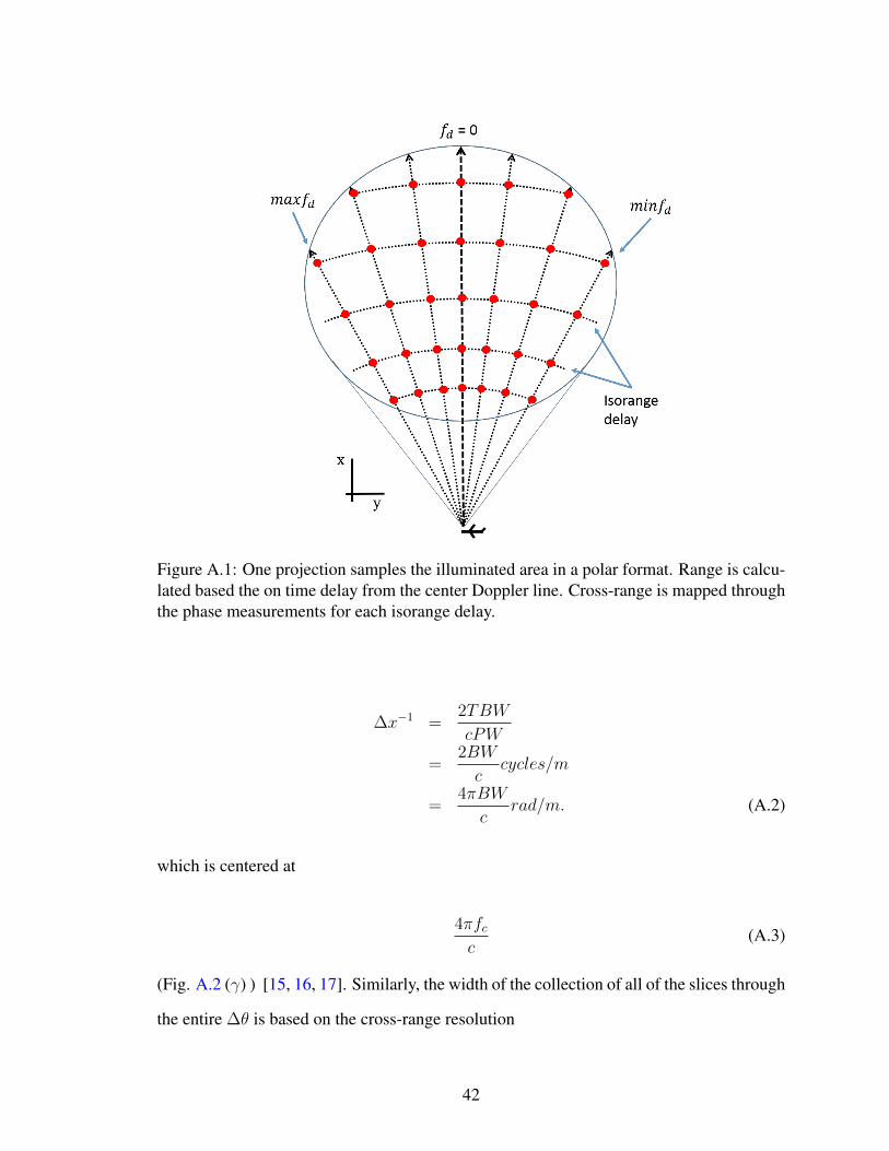
Figure A.1: One projection samples the illuminated area in a polar format. Range is calcu-lated based the on time delay from the center Doppler line. Cross-range is mapped throughthe phase measurements for each isorange delay.
∆x−1 =2TBW
cPW
=2BW
ccycles/m
=4πBW
crad/m. (A.2)
which is centered at
4πfcc
(A.3)
(Fig. A.2 (γ) ) [15, 16, 17]. Similarly, the width of the collection of all of the slices through
the entire ∆θ is based on the cross-range resolution
42
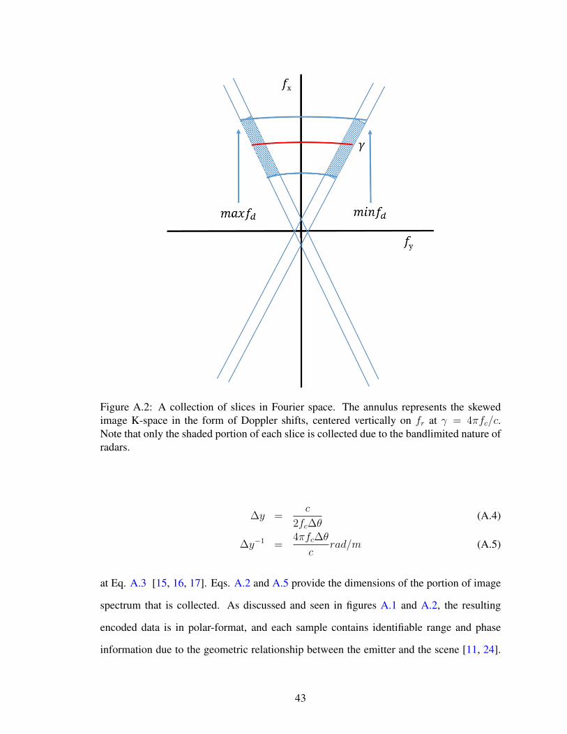
Figure A.2: A collection of slices in Fourier space. The annulus represents the skewedimage K-space in the form of Doppler shifts, centered vertically on fr at γ = 4πfc/c.Note that only the shaded portion of each slice is collected due to the bandlimited nature ofradars.
∆y =c
2fc∆θ(A.4)
∆y−1 =4πfc∆θ
crad/m (A.5)
at Eq. A.3 [15, 16, 17]. Eqs. A.2 and A.5 provide the dimensions of the portion of image
spectrum that is collected. As discussed and seen in figures A.1 and A.2, the resulting
encoded data is in polar-format, and each sample contains identifiable range and phase
information due to the geometric relationship between the emitter and the scene [11, 24].
43
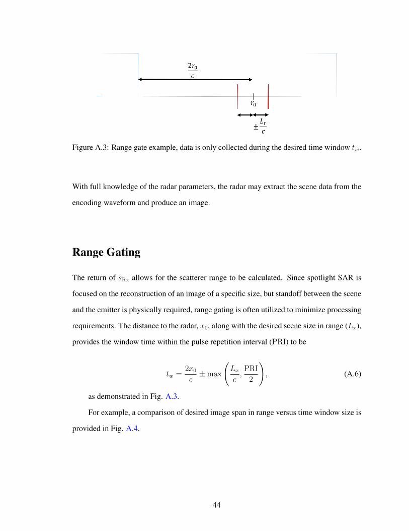
Figure A.3: Range gate example, data is only collected during the desired time window tw.
With full knowledge of the radar parameters, the radar may extract the scene data from the
encoding waveform and produce an image.
Range Gating
The return of sRx allows for the scatterer range to be calculated. Since spotlight SAR is
focused on the reconstruction of an image of a specific size, but standoff between the scene
and the emitter is physically required, range gating is often utilized to minimize processing
requirements. The distance to the radar, x0, along with the desired scene size in range (Lx),
provides the window time within the pulse repetition interval (PRI) to be
tw =2x0
c±max
(Lxc,PRI
2
), (A.6)
as demonstrated in Fig. A.3.
For example, a comparison of desired image span in range versus time window size is
provided in Fig. A.4.
44

Figure A.4: Tw bounds for range gating based on desired scene size Lx, x0 = 10 km.
45
Appendix B
Linear Frequency Modulated Waveform
Parameters
SAR was first developed through the observation that at any time t, an individual point
scatterer will provide a unique Doppler shift (fd) due to the variation of the emitter velocity
relative to each scatterer
fd =2vfc cos(θc)
c(B.1)
where v, θc, fc, and c represent the velocity, cone angle, carrier frequency, and speed of
light, respectively; which is utilized by some A [22]. Disregarding any moving scatterers
in the scene relative to the ground, the desired scene size in cross-range (Ly) determines
the angular deviation (∆θ) for each cross-range bin and therefore the effective bandwidth
(βeff ) for that scene (Fig. B.1(b)).
∆θ = sin−1
(Lxx0
)(B.2)
βeff =2vfc cos(θc ±∆θ)
c(B.3)
Since longer collect ranges are inversely proportional to ∆θ, the desired ∆CR may
46
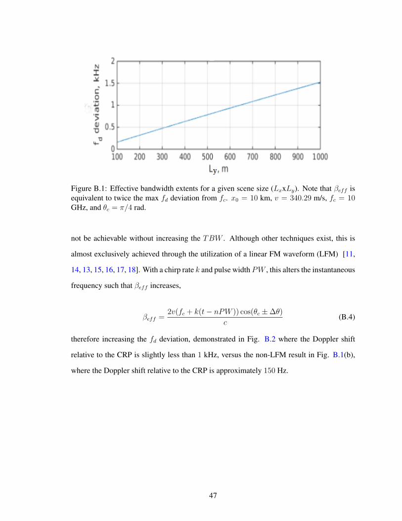
Figure B.1: Effective bandwidth extents for a given scene size (LxxLy). Note that βeff isequivalent to twice the max fd deviation from fc. x0 = 10 km, v = 340.29 m/s, fc = 10GHz, and θc = π/4 rad.
not be achievable without increasing the TBW . Although other techniques exist, this is
almost exclusively achieved through the utilization of a linear FM waveform (LFM) [11,
14, 13, 15, 16, 17, 18]. With a chirp rate k and pulse width PW , this alters the instantaneous
frequency such that βeff increases,
βeff =2v(fc + k(t− nPW )) cos(θc ±∆θ)
c(B.4)
therefore increasing the fd deviation, demonstrated in Fig. B.2 where the Doppler shift
relative to the CRP is slightly less than 1 kHz, versus the non-LFM result in Fig. B.1(b),
where the Doppler shift relative to the CRP is approximately 150 Hz.
47
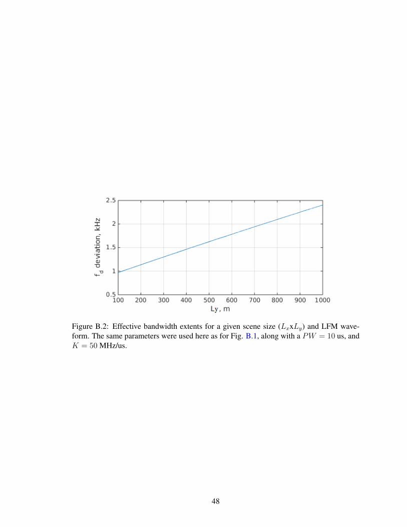
Figure B.2: Effective bandwidth extents for a given scene size (LxxLy) and LFM wave-form. The same parameters were used here as for Fig. B.1, along with a PW = 10 us, andK = 50 MHz/us.
48
Appendix C
SAR Processing Model
1. Sampling: sRx is sampled at some rate ∆tf that satisfies the Nyquist sampling re-
quirement of sTx such that the samples form a sampling index tn.
2. Demodulation and Shaping: Many image formation processes utilize demodulation-
on-receive in order to minimize computational cost. Regardless, the data is then
shaped into a 2D fast-time, slow-time map (sRx(tf , ts)). The combination of the PRI
and tn provides the indices for the fast-time and slow-time [11]. Although the emit-
ter is constantly traveling, for simplicity it is assumed that for each individual PRI
the emitter remains static. This implies a general physical position, velocity, and
acceleration analysis being evaluated only along the ts index. Further, this allows
ts and θ to be used interchangeably. sRx(tf , ts) is formed in order to facilitate im-
age formation through manipulation of the information history afforded by Fourier
and/or correlation theory.
3. Image Formation Algorithm: An image formation algorithm (A) is utilized in order
to extract the information encoded in sRx(tf , ts) and focus the data to a general ’top-
down’ viewpoint image (ψ) such that
ψ(tf , ts) = A(sRx(tf , ts)). (C.1)
49
The method used for the examples in this paper is the downsampled matched filter
(DMF). This method generates the physical model response individually for a tar-
get at each pixel, such that for an NxM image there will be NM forward model
response generations. The value estimated for each pixel is the result of the squared
dot product of the received fast-time, slow-time map and the corresponding individ-
ual forward model response (sM ) [19]. This value represents the radar cross section
of the pixel area in proportion to the rest of the map. This method does not directly
remap the coordinate system to Cartesian to utilize traditional processing, but calcu-
lates the correlation of the received data and a possible reflector at each pixel such
that
ψ(x0, y0) = −→sRx(ρ, sTx,K) • −→sM(δ(x− x0,y − y0), sTx,K). (C.2)
4. Autofocus: It is common for errors to be present in the data which may be space-
invariant and/or space-variant. Typically an autofocus technique (a) is utilized in
order to form the final focused image ρ through
ρ = a(ψ). (C.3)
For example, one common autofocus technique is the Map Drift Algorithm which
is primarily utilized to account for errors in K. It functions through finding some
correction coefficient ∆err by finding the displacement from zero of the maximum
of
ψ1 ? ψ2 (C.4)
where ψ1 and ψ2 represent halves of the data (subapertures) with respect to the
desired axis and ? represents cross-correlation. For side-looking radar, since the
50
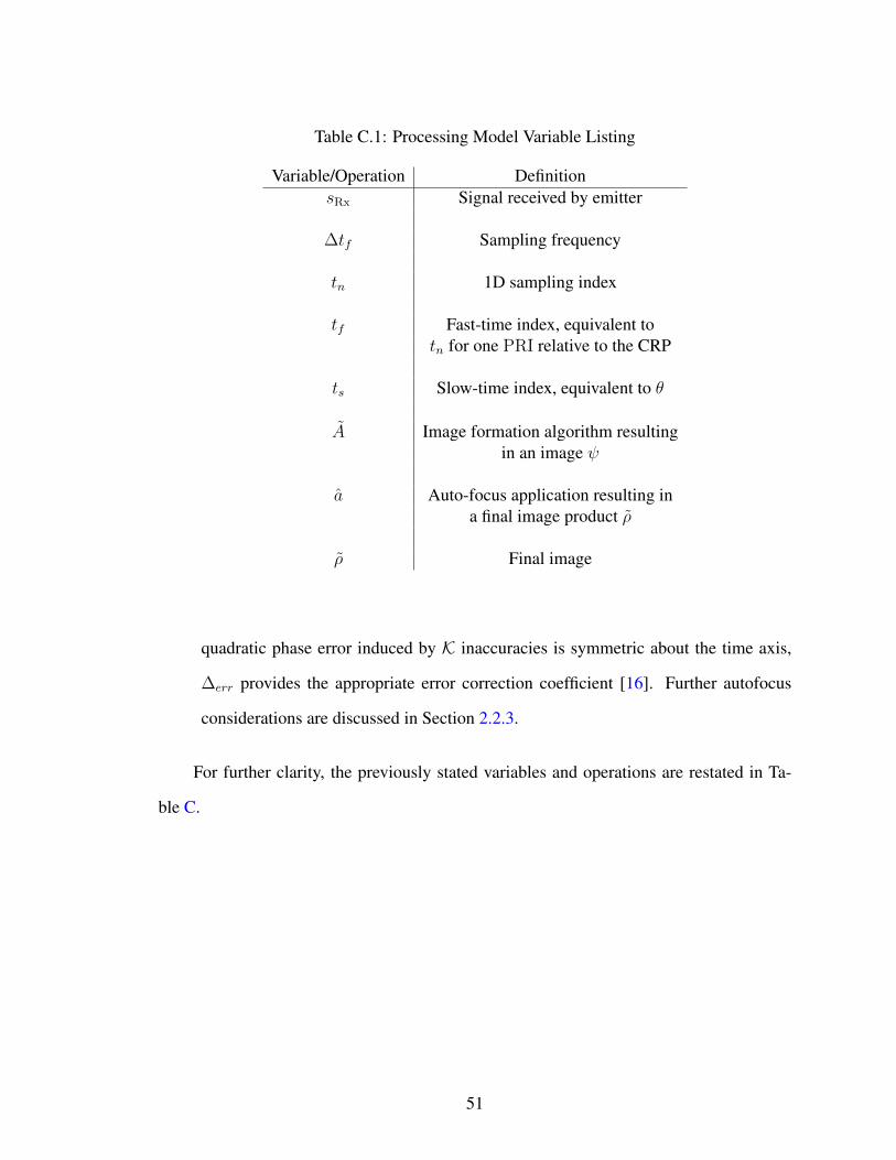
Table C.1: Processing Model Variable Listing
Variable/Operation DefinitionsRx Signal received by emitter
∆tf Sampling frequency
tn 1D sampling index
tf Fast-time index, equivalent totn for one PRI relative to the CRP
ts Slow-time index, equivalent to θ
A Image formation algorithm resultingin an image ψ
a Auto-focus application resulting ina final image product ρ
ρ Final image
quadratic phase error induced by K inaccuracies is symmetric about the time axis,
∆err provides the appropriate error correction coefficient [16]. Further autofocus
considerations are discussed in Section 2.2.3.
For further clarity, the previously stated variables and operations are restated in Ta-
ble C.
51
Appendix D
Jaccard Distance Examples
The Jaccard Distance, or shared information distance, satisfies the fundamental require-
ments as an image similarity metric, which are the following: the identity axiom, the tri-
angle inequality, the symmetry axiom, and its value is always positive [31, 32]. In order
to provide some level of intuition into the magnitude of the Jaccard Distance between an
image A and a modified version of that image, B, as B degrades from A, translational,
rotational, and combined sweeps of the offsets between A and B are shown in Fig. D.1.
Further, Fig. D.2 shows the histogram of the Jaccard Distance for 1000 Monte Carlo trials
for
D(A,B)∣∣∣B=A+n
(D.1)
where
n ∼ N (0, 0.22) w.g.n. (D.2)
52
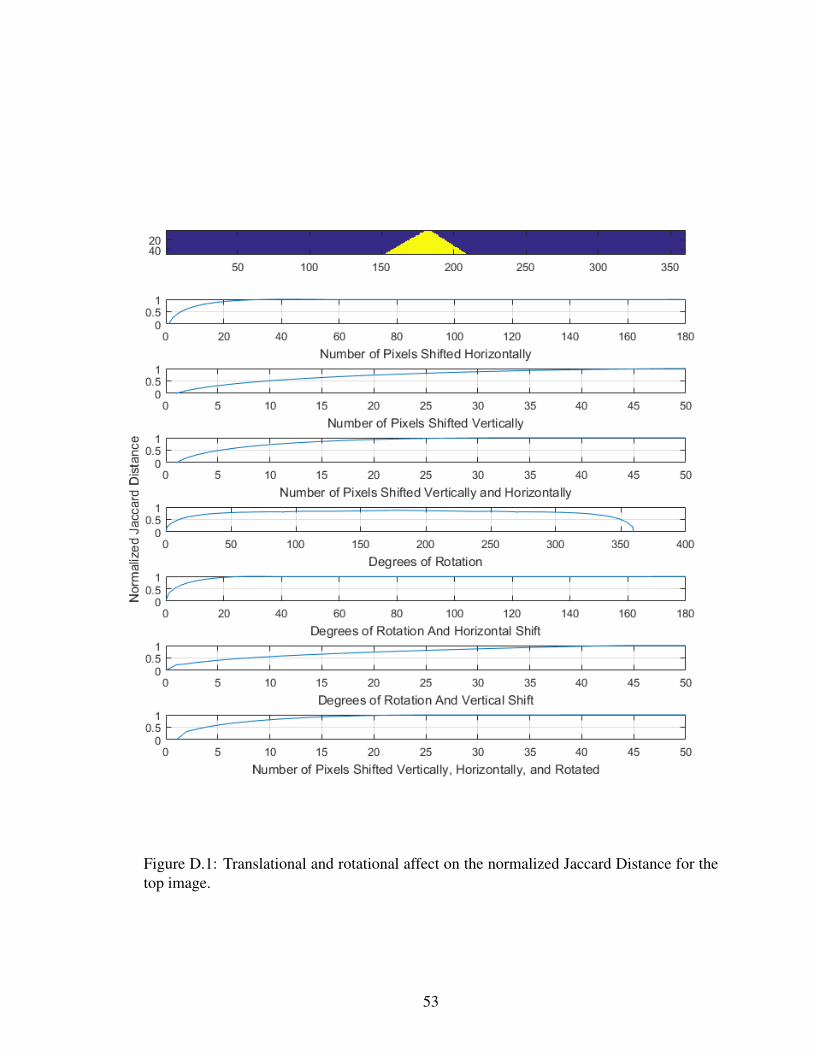
Figure D.1: Translational and rotational affect on the normalized Jaccard Distance for thetop image.
53
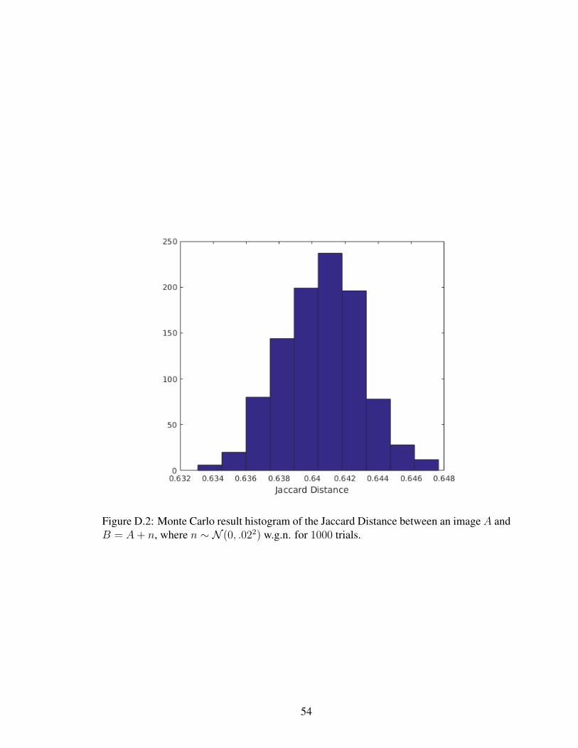
Figure D.2: Monte Carlo result histogram of the Jaccard Distance between an image A andB = A+ n, where n ∼ N (0, .022) w.g.n. for 1000 trials.
54
Appendix E
Linear Frequency Modulated Waveform
Model and Processing
The transmitted LFM waveform
sTx(t) = A0p(t)e−jΦ(t) (E.1)
Φ(t) = 2πf0t+ πkt2, (E.2)
where t, p, A0, f0, and k denote time, pulse envelope, amplitude, carrier frequency, and
chirp rate, respectively. sTx interacts with the scene reflectivity density ρ such that a portion
of the signal energy is reflected back towards the emitter, and may be modeled with some
time shift τ such that the signal received by the radar sRx is
sRx = ρ(t− τ) ∗ sTx(t− τ). (E.3)
Applying the standard 2-way range equation
t =2r
c, (E.4)
55
where r is the range and c is the speed of light, to Eq. (E.3) provides
sRx = ρ(r) ∗ sTx(t−2r
c). (E.5)
Showing the scene reflectivity density ρ as N scatterers
ρ(r) = Anδ(r − rn) (E.6)
allows Eq. (E.5) to be represented as
sRx = ρ(r) · sTx(t) (E.7)
= Anδ(r − rn) · sTx(t− 2r
c
)(E.8)
= AnsTx
(t− 2rn
c
)(E.9)
= AnA0p(t− 2rn
c
)ej2πf0
(t− 2rn
c
)+jπk
(t− 2rn
c
)2. (E.10)
The kinematic model of the radar K is represented through
r − rn =√
(x− xn)2 + (y − yn)2 + (z − zn)2 (E.11)
and therefore the scene ρ may be shown as relative to the radar’s K as
ρ(x, y, z) = Anδ(x− xn)δ(y − yn)δ(z − zn). (E.12)
56
Processing the received signal with a matched filter provides the result y(t) through
y(t) = sRx(t) ∗ s∗Tx(t− 2r0
c
)(E.13)
= AnA0p(t− 2rn
c
)ejΦ(t− 2rn
c
)· A−1
0 p(t− 2r0
c
)e−jΦ
(t− 2r0
c
)(E.14)
= Anp(t− 2r0
c
)ej2πfc
(t− 2rn
c
)+jπk
(t− 2rn
c
)2× ej2πfc
(t− 2r0
c
)+jπk
(t− 2r0
c
)2(E.15)
= Anp(t− 2r0
c
)ej(
4πfcc
(r0−rn)+ 4πktc
(r0−rn)+ 4πkc2
(r2n−r20))
(E.16)
Expanding the range terms provides that
(r2n − r2
0) = (r2n − 2rnr0 + r2
0) + 2rnr0 − 2r20
= (rn − r0)2 + 2rnr0 − 2r20 (E.17)
y(t) = Anp(t− 2r0
c
)ej
4πc
(fc+kt)(r0−rn)+k((rn−r0)2+2rnr0−2r20 . (E.18)
The deramp process produces
y(t) = Anp(t− 2r0
c
)ej
4πc
(fc+kt)(r0−rn)+k((rn−r0)2
= Anp(t− 2r0
c
)e−j
4πc
(fc+kt)(rn−r0)−k((rn−r0)2 , (E.19)
which may be simplified and written to isolate the time dependent terms through
t′ = t− 2r0
c(E.20)
∆r = rn − r0 (E.21)
y(t′) =(p(t′)e−j
4πkt′c
∆r)(Ane
−j 4πfcc
∆r+j 4πkc2
∆r2). (E.22)
57
The spectrum of the processed signal provides the superimposed Doppler shifts which are
typically mapped to cross-range locations. The spectrum of y is found through
Y (ζ) = F{y(t′)} (E.23)
=
∫ ∞−∞
y(t′)e−jζt′∂t′ (E.24)
= Ane−j 4πfc
c∆r+j 4πk
c2∆r2∫ ∞−∞
p(t′)e−j4πkt′c
∆re−jζt′∂t′. (E.25)
The spectrum Y is further simplified by allowing
ζn =4πk∆r
cs.t. (E.26)
Y (ζ) = Ane−j 4πfc
c∆r+j 4πk
c2∆r2∫ ∞−∞
p(t′)e−jζnt′e−jζt
′∂t′. (E.27)
If a rectangular pulse is assumed,
Y (ζ) = Ane−j 4πfc
c∆r+j 4πk
c2∆r2sinc(ζ)δ(ζ − ζn) (E.28)
= Ane−j 4πfc
c∆r+j 4πk
c2∆r2sinc(ζ − ζn), (E.29)
and a single ζn produces
|Y (ζn)| = Ansinc(ζ − ζn). (E.30)
The width of the sinc(ζ) mainlobe is the range resolution δr as shown in Eq. (A.1), which
may also be shown with Eq. (E.26) through
δζ =2π
PW=
4πkδr
c(E.31)
δr =c
2kPW=
c
2BW. (E.32)
The velocity of a scatterer ~vg relative to the velocity of the radar ~vr creates a Doppler
shift fd in sTx when incident with the scatterer. The phase of the received signal, from
58
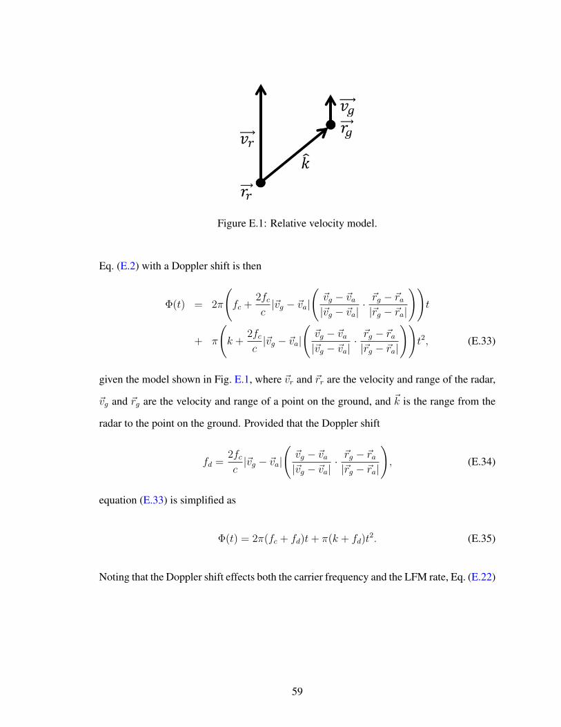
Figure E.1: Relative velocity model.
Eq. (E.2) with a Doppler shift is then
Φ(t) = 2π
(fc +
2fcc|~vg − ~va|
(~vg − ~va|~vg − ~va|
· ~rg − ~ra|~rg − ~ra|
))t
+ π
(k +
2fcc|~vg − ~va|
(~vg − ~va|~vg − ~va|
· ~rg − ~ra|~rg − ~ra|
))t2, (E.33)
given the model shown in Fig. E.1, where ~vr and ~rr are the velocity and range of the radar,
~vg and ~rg are the velocity and range of a point on the ground, and ~k is the range from the
radar to the point on the ground. Provided that the Doppler shift
fd =2fcc|~vg − ~va|
(~vg − ~va|~vg − ~va|
· ~rg − ~ra|~rg − ~ra|
), (E.34)
equation (E.33) is simplified as
Φ(t) = 2π(fc + fd)t+ π(k + fd)t2. (E.35)
Noting that the Doppler shift effects both the carrier frequency and the LFM rate, Eq. (E.22)
59
may be used to show both the time and frequency shifts as
y(t′) = Anp(t′)e−j
4π(k+fd)t′
c∆r−j 4π(fc+fd)
c∆r+j
4π(k+fd)
c2∆r2 (E.36)
= Anp(t′)e−j2π(k+fd)t′∆t−j2π(fc+fd)∆t+jπ(k+fd)∆t2 (E.37)
= Anp(t′)e−j2π(fc+fd)∆t−j2π(k+fd)t′∆t+jπ(k+fd)∆t2 . (E.38)
Equation (E.38) provides a typical expression for the matched filter result of an LFM signal,
where the left third of the phase contains all of the needed scene information to locate the
scatterer. The remaining phase terms make up the well known residual video phase, which
may be corrected [13, 15, 16, 18].
60


![Kinematic model for quasi static granular displacements … · International Journal of Rock Mechanics & Mining Sciences ] (]]]]) ]]]–]]] Kinematic model for quasi static granular](https://static.fdocuments.us/doc/165x107/5ba61e9b09d3f22c448b7cff/kinematic-model-for-quasi-static-granular-displacements-international-journal.jpg)
![[PPT]SCARA – Forward Kinematics - Zimtok5.com - Home · Web viewSCARA – Forward Kinematics Use the DH Algorithm to assign the frames and kinematic parameters SCARA – Forward](https://static.fdocuments.us/doc/165x107/5b2123fa7f8b9a9b0a8b466a/pptscara-forward-kinematics-home-web-viewscara-forward-kinematics.jpg)