Effects of subsampling of passive acoustic recordings on ... et al... · Effects of subsampling of...

Effects of subsampling of passive acoustic recordingson acoustic metrics

Karolin Thomisch,a) Olaf Boebel, and Daniel P. ZitterbartOcean Acoustics Lab, Alfred-Wegener-Institut Helmholtz Zentrum f€ur Polar- und Meeresforschung,27570 Bremerhaven, Germany

Flore SamaranObservatoire PELAGIS CNRS–UMS 3462, University of La Rochelle, 17000 La Rochelle, France

Sofie Van ParijsNortheast Fisheries Science Center, 166 Water Street, Woods Hole, Massachusetts 02543, USA

Ilse Van OpzeelandOcean Acoustics Lab, Alfred-Wegener-Institut Helmholtz Zentrum f€ur Polar- und Meeresforschung,27570 Bremerhaven, Germany

(Received 2 March 2015; accepted 5 June 2015; published online 15 July 2015)

Passive acoustic monitoring is an important tool in marine mammal studies. However, logistics and

finances frequently constrain the number and servicing schedules of acoustic recorders, requiring a

trade-off between deployment periods and sampling continuity, i.e., the implementation of a

subsampling scheme. Optimizing such schemes to each project’s specific research questions is

desirable. This study investigates the impact of subsampling on the accuracy of two common

metrics, acoustic presence and call rate, for different vocalization patterns (regimes) of baleen

whales: (1) variable vocal activity, (2) vocalizations organized in song bouts, and (3) vocal activity

with diel patterns. To this end, above metrics are compared for continuous and subsampled data

subject to different sampling strategies, covering duty cycles between 50% and 2%. The results

show that a reduction of the duty cycle impacts negatively on the accuracy of both acoustic

presence and call rate estimates. For a given duty cycle, frequent short listening periods improve

accuracy of daily acoustic presence estimates over few long listening periods. Overall, subsampling

effects are most pronounced for low and/or temporally clustered vocal activity. These findings

illustrate the importance of informed decisions when applying subsampling strategies to passive

acoustic recordings or analyses for a given target species. VC 2015 Author(s). All article content,except where otherwise noted, is licensed under a Creative Commons Attribution 3.0 UnportedLicense. [http://dx.doi.org/10.1121/1.4922703]

[JFL] Pages: 267–278

I. INTRODUCTION

Passive acoustic monitoring (PAM) is a widely used tool

in marine mammal research concerning primarily spatio-

temporal distribution patterns and behavior of vocalizing spe-

cies (e.g., Mellinger et al., 2007; Van Parijs et al., 2009; Van

Opzeeland et al., 2010). Recent methodological advances

have broadened the field of PAM applications to also include

abundance estimations for some marine mammals (K€usel

et al., 2011; Marques et al., 2011; Ward et al., 2012; Harris

et al., 2013). While dependent on vocalizations from the tar-

get species, PAM exhibits several advantages over traditional

visual surveys, such as the possibility to collect data under

poor weather conditions, during darkness and in areas with

dense ice cover, allowing marine mammal monitoring in

regions and at times otherwise inaccessible (both logistically

and financially) (e.g., Mellinger et al., 2007). In particular,

autonomous passive acoustic recorders are the tool of choice

for collecting long-term data series in remote areas that are

inaccessible to ships during much of the year, such as the

Arctic and Southern Oceans (e.g., �Sirovic et al., 2009;

Samaran et al., 2010; Stafford et al., 2012; Sousa-Lima et al.,2013; Van Opzeeland et al., 2013). In many cases, logistic

and financial constraints determine the frequency at which

recorders are serviced, resulting in time spans of up to two to

three years between recorder deployment and retrieval (e.g.,�Sirovic et al., 2004; Miksis-Olds et al., 2010; Rettig et al.,2013). However, to date, the majority of autonomous record-

ing instruments do not quite feature sufficient capacity in

terms of battery life and/or data storage to record continu-

ously for such prolonged deployment periods at high sam-

pling rates (e.g., Rettig et al., 2013).

Nevertheless, as multi-year data are indispensable to

capture long-term trends in temporal and seasonal occur-

rences of species, full coverage of the period between

recorder deployment and retrieval is highly desirable.

This often requires recordings to be subsampled (e.g.,

Burtenshaw et al., 2004; Gedamke et al., 2007; Stafford

et al., 2012; Rettig et al., 2013), i.e., to be collected at a re-

petitive pattern of sampling periods and non-sampling

periods at a given repetition cycle. Likewise, for humana)Electronic mail: [email protected]

J. Acoust. Soc. Am. 138 (1), July 2015 VC Author(s) 2015 2670001-4966/2015/138(1)/12/10

Redistribution subject to ASA license or copyright; see http://acousticalsociety.org/content/terms. Download to IP: 24.218.226.58 On: Thu, 16 Jul 2015 12:46:59

http://dx.doi.org/10.1121/1.4922703

mailto:[email protected]

http://crossmark.crossref.org/dialog/?doi=10.1121/1.4922703&domain=pdf&date_stamp=2015-07-01

screening of comprehensive, continuous data sets, research-

ers may resort to analyzing subsets of the data to accelerate

the analysis process (e.g., Oleson et al., 2007; Van

Opzeeland et al., 2010).

Subsampling of a given percentage of time might, how-

ever, be implemented in different ways, with the extremes

being either many short listening periods (sampling bouts) or

few long listening periods. This option immediately gives

rise to the question of potential impacts of the subsampling

scheme on ecological inferences drawn from the ensuing

data which, in turn, leads to the question for the most suita-

ble sampling scheme for a given species. Simply put, if the

recording period is limited, for example, to 1 h during a day,

one wonders whether sampling once daily for an hour, twice

daily for half an hour, or four times a day for 15 min repre-

sents the vocal behavior of a given species best.

The choice of a specific subsampling scheme will be

driven by the research question, power and storage capacity

of the recording equipment and most importantly the desire

not to introduce any biases to the data which can be achieved

by seeking an optimal sampling scheme based on pre-

existing knowledge on vocalization patterns (e.g., Sousa-

Lima et al., 2013). Impacts of subsampling are likely to

depend strongly on the characteristics of the focal species’

vocal behavior: In case of frequent, regular calls, results

from subsampled data may remain representative of the

respective period. However, if vocal activity occurs rarely or

exhibits a distinct diurnal pattern, sampling exclusively at

off-periods would result in substantial misrepresentations of

the focal species’ acoustic presence. Consequently, suitable

subsampling requires tuning to the acoustic behavior of

the focal species, such as rate and temporal structure of call

production.

Acoustic presence (a binary parameter) and call rate

(a continuous numeric parameter) are two frequently used

metrics to investigate various aspects of marine mammal

ecology (e.g., Mellinger et al., 2007; �Sirovic et al., 2007;

Van Opzeeland et al., 2013), such as spatio-temporal pat-

terns in occurrence and distribution, locations of feeding or

overwintering habitats as well as density estimations (see

also Table I and references therein). In turn, an unbiased

assessment of a focal species’ acoustic presence is essential

for descriptions of its occurrence and distribution on spatial

and/or temporal scales (Table I).

Continuous passive acoustic recordings of North

Atlantic right whales (NARW, Eubalaena glacialis) and

Antarctic blue whales (ABW, Balaenoptera musculus inter-media) were used in this study to investigate the potential

impacts of different subsampling schemes on acoustic pres-

ence and call rates by comparing the ensuing results with

regard to their representativeness.

II. MATERIALS AND METHODS

A. Passive acoustic data acquisition

Continuous passive acoustic data were collected at three

different locations. On the Ekstr€om ice shelf at 70� 310 S, 8�

130 W, the PerenniAL Acoustic Observatory in the Antarctic

Ocean (PALAOA) collects continuous underwater record-

ings from a coastal Antarctic environment since 2005 with a

Reson TC4032 hydrophone, deployed at approximately

160 m depth (Boebel et al., 2006; Kindermann et al., 2008).

In the Indian Ocean, southwest of Amsterdam Island

(‘SWAMS’, 42� 590 S, 74� 350 E), continuous acoustic record-

ings were collected from October 2006 to April 2008 with an

ITC-1032 hydrophone moored at 1000 m depth (see Samaran

et al., 2013 for further details). In Massachusetts Bay, MA,

continuous acoustic data were recorded from January 2006 to

February 2007 by means of marine autonomous recording

units (MARUs) deployed at depths ranging from 41 to 76 m

TABLE I. Acoustic parameters used in the present case study and possible inferences on the focal species’ ecology based on these parameters as reported by

previous studies.

Parameter Direct and further inferences References (exemplary)a

Acoustic presence Occurrence of a focal species at recording location(s)

with potential indications on suitability of habitat for

overwintering/breeding/feeding/etc.

(Mussoline et al., 2012; Rankin et al., 2005; Samaran et al.,2013; �Sirovic et al., 2009; Stafford et al., 2004)

Spatial and temporal patterns in distribution of focal species

in certain area

(Gedamke et al., 2007;b Matthews et al., 2014; Mussoline

et al., 2012; Samaran et al., 2013; �Sirovic et al., 2004)

Diel vocalization patterns (Mussoline et al., 2012)

Associations with abiotic or biotic factors (Burtenshaw et al., 2004)b

Vocalization rate Abundance and density estimations of animals at recording

location/in study area

(Marques et al., 2013; �Sirovic et al., 2004)

Estimation of historical catch numbers of different blue

whale populations from calling patterns

(Monnahan et al., 2014)

Movement/migration patterns of animals (Samaran et al., 2013; �Sirovic et al., 2004; �Sirovic et al.,2009)

Diel vocalization patterns (Matthews et al., 2014; Stafford et al., 2005; Wiggins et al.,2005)

Associations with abiotic or biotic factors (�Sirovic et al., 2004; �Sirovic and Hildebrand, 2011)

Effects of anthropogenic noise on focal species (Di Iorio and Clark, 2010; McDonald et al., 1995; Melc�on

et al., 2012)

aReferences were selected exemplarily, mainly representing passive acoustic research on the focal species of this study, i.e., blue whale (Balaenoptera muscu-lus) and North Atlantic right whale (Eubalaena glacialis).bStudies based on subsampled acoustic data.

268 J. Acoust. Soc. Am. 138 (1), July 2015 Thomisch et al.


at 10 separate locations throughout the Stellwagen Bank

National Marine Sanctuary (see Mussoline et al., 2012 for

further details).

B. Focal species and vocalizations

The continuous passive acoustic recordings used in this

study contained a variety of marine mammal sounds, yet

only ABW Z-calls and NARW up-calls are examined herein.

ABW Z-calls (Fig. 1) consist of three components, starting

with a constant frequency tone at 27 Hz which lasts for about

8–12 s, followed by a short downsweep to 19 Hz of about

1–2 s duration and a longer (8–12 s) slightly frequency

modulated tone at about 18–19 Hz (e.g., Ljungblad et al.,1998; Rankin et al., 2005). The NARW’s up-call is a fre-

quency modulated call lasting approximately 1 s with an

increasing frequency from 50 to 200 Hz (Fig. 1), which is

considered to serve as contact call (Clark, 1982; Parks and

Clark, 2007).

C. Passive acoustic data sets

Five data subsets, each comprising seven days, were

extracted from the three continuous data sets described in

Sec. II A. Each subset is representative of a different pattern

of calling behavior including: (1) variable acoustic activity,

(2) clear song sequences, and (3) vocal activity featuring a

clear diel pattern.

1. Variable, temporally unstructured acoustic activitywith both high and low calling rates

To explore how subsampling may affect data featuring

variable acoustic activity, i.e., without any clear song pattern

or diurnal trend, two sets from the PALAOA data were cho-

sen on the basis of results from previous analyses of seasonal

vocal activity of Antarctic blue whales (Van Opzeeland,

2010) (Fig. 2). Generally, Z-calls are considered to be

repeated every 60 to 65 s in patterned sequences (“song”)

(e.g., Ljungblad et al., 1998; �Sirovic et al., 2004), however,

clear song sequences were not present in this selection of

PALAOA data. Instead, the acoustic activity was variable

with periods of higher and lower calling activity. The

selected data were resampled at 6 kHz and ABW Z-call

detection was performed visually by manually screening 1-

min spectrograms (FFT 8,192 points, Hanning window,

time, and frequency resolution 1.3 s, 0.75 Hz) with Adobe

Audition 2.0, resulting in call count data at 1-min resolution.

“Regime A–high call rate” represented high vocal activity of

an average of 55 6 18 (standard deviation) Z-calls per hour,

whereas “regime B–low call rate” represented data with me-

dium vocal activity of 20 6 8 Z-calls per hour on average.

FIG. 1. Spectrogram of Antarctic blue

whale Z-call (left panel) and North

Atlantic right whale up-call vocal-

ization (right panel). Sound file of

NARW up-call was downloaded

from http://www.nefsc.noaa.gov/psb/

acoustics/sounds.html.

FIG. 2. Passive acoustic data sets used for exploring the effects of different subsampling schemes on call rate and acoustic presence estimation.

J. Acoust. Soc. Am. 138 (1), July 2015 Thomisch et al. 269


http://www.nefsc.noaa.gov/psb/acoustics/sounds.html

http://www.nefsc.noaa.gov/psb/acoustics/sounds.html

No diurnal patterns were evident in these data. Data sets

comprised four consecutive days from January and three

consecutive days from February (1–4 January 2012 and 1–3

February 2012) for regime A and three consecutive days

from June and four consecutive days from July (9–11 June

2012 and 1–4 July 2012) for regime B (Fig. 2). The number

of consecutive days was constrained by the presence of noisy

periods on some days, caused, for example, by glacier calv-

ing. Noisy days were excluded as these potentially affected

the reliability of call counts.

2. Structured acoustic activity with clear songsequences by single and multiple individuals

The Indian Ocean data contained sequences of ABW

Z-call vocalizations organized in regular song structures.

Calls were automatically detected using a template detec-

tor in XBAT (Figueroa and Robbins, 2008; see Samaran

et al., 2013 for further details). ABW Z-call song featuring

inter-call intervals of 60–65 s typically stem from a single

calling individual (e.g., �Sirovic et al., 2004) and such

events were hence considered as representing single sing-

ers. Periods with shorter inter-call intervals are representa-

tive of the presence of multiple singers. Seven consecutive

recording days from June 2007 (18–24 June 2007) con-

taining individual song were selected to form “regime

C–single song,” with 17 6 8 Z-calls per hour on average

(Fig. 2). “Regime D–multiple song” comprised a second

set of seven consecutive days (23–29 August 2007, Fig. 2)

of continuous recordings with 35 6 22 Z-calls per hour on

average, containing ABW song sequences with shorter

inter-call intervals (with �30% of inter-call intervals rang-

ing between 15 and 45 s). No diurnal patterns were evident

in these data.

3. Call activities exhibiting strong diel patterns

The Stellwagen Bank acoustic data, containing NARW

vocalizations, were analyzed in XBAT, using a custom-

written automated call detection algorithm to detect NARW

up-calls (see Mussoline et al., 2012 for further details).

Seven consecutive recording days (6–12 April 2006, repre-

senting pooled call detections from nine different locations)

with distinct diel fluctuations [i.e., increased NARW vocal

activity during twilight and at night (Mussoline et al., 2012)]

were selected to comprise “regime E–diel patterns” (Fig. 2).

Hourly call rates ranged from 0 to 137 up-calls per hour

(mean 12 6 6 up-calls per hour).

D. Subsampling schemes

Subsampling schemes are defined by their cycle periods(sc, “sampling intervals”) and duty cycles D, commonly

given in percent but as a fractional number hereinafter

(Table II and Fig. 3) The corresponding listening period sl

(i.e., length of a sampling bout) is then given by sl ¼ D � sc.

In the course of a day, the cycle is repeated 24 h=sc ¼ Ntimes (number of cycles per day), with sc usually chosen

such that N 2N (Fig. 3).

The potential repercussions of different sampling

schemes are explored in this publication by varying (a) the

cycle period (sc) (or correspondingly the number of cyclesper day N) and (b) the duty cycle D. Table III lists the ana-

lyzed combinations of cycling periods and duty cycles that

result in full minute listening periods. A given duty cycle Dmay be realized differently in terms of cycle period and

corresponding listening period (rows of Table III), resulting

in different sampling strategies (e.g., a single long listening

period versus multiple shorter windows distributed evenly

over the course of a day).

In PAM studies, commonly little consideration is given

to when exactly a cycle period commences within a day,

while the start of a listening period mostly matches that of

the corresponding cycle period. However, (phase) shifts

of either are feasible. Within a cycle period (sc) the number

of independent (non-overlapping) listening periods equals

1/D, called the number or realizations r hereinafter (Fig. 3).

For our statistical analysis of the effects of data subsampling,

all possible 1/D realizations were processed to estimate the

variability of call rates and acoustic presence estimations

(Table II). This procedure provided 7=D (1/D realizations

times seven days) independent estimates of acoustic pres-

ence and call rates per regime, respectively.

1. Daily acoustic presence estimationsfrom subsampled data

For continuous data, a species was considered present if

at least one call was evident during a day. For subsampled

data, a focal species was considered acoustically present if at

TABLE II. Index of abbreviations and symbols.

Symbol Definition

sc Cycle period [h], i.e., the interval at which data collection is repeated

N Number of cycles per day

sl Duration of listening period [min], i.e., the period over which data are acquired continuously

D ¼ sl / sc; duty cycle

1/D ¼ sc / sl; number of independent realizations of a given sampling scheme, i.e., number of listening periods per cycle

d Metric depicting correctness of acoustic presence determination in subsampled data compared to true acoustic presence in continuous data;

d¼ 1 representing correct acoustic presence estimation and d¼ 0 representing incorrect acoustic presence estimation

pp Probability to correctly assess acoustic presence of a focal species during the day

pc Probability to assess call rate of a focal species within a certain range (i.e., 10%, 50%, and 100%, respectively) of the true call rate



least one call was detected in any of the N listening periods

of that day (Table III). Daily acoustic presence was esti-

mated from the call counts in the rth realization in all Ncycles of the jth day. If the assessments of acoustic presence

from subsampled data and from continuous data matched,

the decision was considered correct (d¼ 1), and incorrect

otherwise (d¼ 0).

To evaluate the probability pp of having properly deter-

mined the acoustic presence during that day, d was deter-

mined for each of the 1/D independent realizations r of the

listening period per day (Table II). This procedure resulted

in 1/D independent estimates dr,j of correctness of presence

assessment per day. The probability pp was calculated from

all 7=D independent dr,j estimates in each acoustic regime,

permitting to establish an average probability of correct

acoustic presence determination and its standard deviation

(n ¼ 7=D) for each sampling scheme:

pp ¼D

7�X7

j¼1

X1=D

r¼1

dr;j: (1)

Between-regime comparisons of the results were conducted

for selected duty cycles (12; 1

4; 1

10; 1

20; and 1

60Þ.

2. Daily call rate estimations from subsampled data

Continuous call count data were subsampled according

to the schemes listed in Table III, and hourly call rates �cwere estimated from the call rates ci of the rth realization in

all N cycles of the jth day:

cr;j ¼1

N

XN

i¼1

ci;r;j: (2)

This estimation was accomplished for all possible realiza-

tions r of listening periods within a cycle providing 1/D in-

dependent daily call rates cr;j per day (Fig. 4).

To assess the variability of call rate estimates within a

given sampling scheme, the ratios of call rates from sub-

sampled data and true call rates from continuous data were

calculated for all cr;j :

ratior;j ¼cr;j � ytrue

ytrue

: (3)

This procedure was repeated for all 1/D ratiosr,j at each day

and resulted in 7=D independent estimates per regime pro-

viding average and standard deviation of call rate estima-

tions at a given subsampling scheme. As animal abundance

estimates from acoustic data strongly depend on the accu-

racy of call rate assessments, the probability pc of estimating

the actual call rate within a range of 10%, 50%, and 100%,

respectively, was calculated (Table II). Results from selected

duty cycles (12; 1

4; 1

10; 1

20; and 1

60Þ were used for between-

regime comparisons.

III. RESULTS

Impacts of different subsampling schemes on daily

acoustic presence were evaluated by determining the proba-

bility of a correct decision regarding acoustic presence.

TABLE III. Listening periods for tested subsampling schemes (i.e., listening period [min] per cycle [h]), representing different duty cycles. Duty cycles high-

lighted in bold indicate subsampling schemes that were used for comparative analyses and interpretation of subsampling effects on passive acoustic data in the

present study.

Duty cycle Cycle period sc

D D [%] 1 h 2 h 3 h 4 h 6 h 8 h 1/D

No. of independent realizations

per regime

1/2 50.0 30 min 60 min 90 min 120 min 180 min 240 min 2 14





1/8 12.5 15 min 30 min 45 min 60 min 8 56

1/9 11.1 20 min 40 min 9 63




1/16 6.3 15 min 30 min 16 112

1/18 5.6 10 min 20 min 18 126


1/24 4.2 5 min 10 min 15 min 20 min 24 168


1/32 3.1 15 min 32 224

1/36 2.8 5 min 10 min 36 252

1/40 2.5 3 min 6 min 9 min 12 min 40 280

1/45 2.2 4 min 8 min 45 315

1/48 2.1 5 min 10 min 48 336


cycles per day N 24 12 8 6 4 3



Subsampling effects on call rate estimates were assessed by

considering the probability of call rate estimates better than

10%, 50%, and 100% of the true call rate.

A. Acoustic presence

Analyses of the continuous data sets reveal that ABWs

were acoustically present on all days in regimes A, B, C, and

D, while NARW up-calls were detected during all days of

regime E. The average time-span of hourly acoustic presence

varied between regimes, with 24 6 0 h of acoustic presence

per day for regime A and B, 19.43 6 5.77 h of acoustic pres-

ence per day for regime C, 23 6 2.24 h of acoustic presence

per day for regime D and 19.14 6 2.41 h of acoustic presence

per day for regime E.

The probability pp to correctly assess daily acoustic

presence of ABWs and NARWs on the basis of subsampled

data was dependent on duty cycle, cycle period and acoustic

regime (Fig. 5). While acoustic presence was always

assessed correctly for high duty cycles (D > 14), small duty

cycles (D � 110

) underestimated the acoustic presence for

some regimes (Fig. 5). Similarly, for a given duty cycle, the

probability of estimating presence correctly was smaller for

long cycles sc (>6 h), i.e., few cycles per day. The repercus-

sions of subsampling also depended strongly on the acoustic

regime, i.e., on the vocalization pattern of the focal species.

For regimes A, B, and D, subsampling had no or only minor

effects on the likelihood of correct presence estimation, even

at small duty cycles (Fig. 5). In regime A, acoustic presence

was always assessed correctly, regardless of the duty cycle,

while in regime B and D presence assessment was correct in

at least 97% of cases for all duty cycles (Fig. 5).

Contrastingly, effects of subsampling were more pronounced

for regimes C and E. While duty cycles of D > 14

did not

affect the probability to correctly estimate acoustic presence,

this probability decreased at smaller duty cycles for both

regimes (Fig. 5). For example, acoustic presence was cor-

rectly assessed with a probability of 73% to 90% at D ¼ 160

for regime E, with probabilities decreasing with increasing

cycle periods (Fig. 5).

FIG. 3. Exemplary scheme of terms used in the context of subsampling of passive acoustic data.

FIG. 4. Exemplary scheme of analysis algorithm to estimate hourly call rates from subsampled passive acoustic data assuming a subsampling scheme of

15 min per hour (DC¼ [1/4]). Upper panel: first run of algorithm estimating hourly call rates in the first 15 min per hour, lower panel: second run of algorithm

estimating hourly call rates in the second 15 min per hour.



B. Call rate estimations

The total number of ABW calls detected in the original

data sets varied between regimes with 9183 calls in regime

A (54.64 6 17.73 calls per hour), 3353 calls in regime B

(19.95 6 7.96 calls per hour), and 2830 (16.85 6 8.81 calls

per hour) and 5823 calls (34.67 6 21.65 calls per hour) in

regimes C and D, respectively. For regime E, 1945 NARW

calls (11.58 6 6.14 calls per hour) were detected.

Call rates based on subsampled data varied significantly

depending on the sampling scheme applied (Fig. 6).

Generally, the variability of call rate estimates increased

with decreasing duty cycle, i.e., call rates based on subsam-

pling with large duty cycles (D > 14) differed less from the

true call rate than call rates based on small duty cycles

(D < 120

) (Fig. 6). For a given duty cycle, increasing cycle

periods sc resulted in a higher variability within the call rate

estimates, i.e., a more widely spread data distribution and

potentially higher deviations from the true call rate (Fig. 6).

While this effect was clearly detectable in regime C, D, and

E, it was less evident in regimes A and B. In turn, effects of

subsampling on call rate estimations also depended strongly

on the vocal behavior of the focal species, i.e., the data

regime analyzed.

In order to quantify the validity of the call rate estimates

from subsampled data, the probability pc that the call rate

estimated from a given subsampling scheme is within a

specified range X (with X being 10%, 50%, and 100%,

respectively) of the true call rate was assessed (Fig. 7). As

expected, the probability to obtain call rate estimates within

a certain range of the true call rate depended on the subsam-

pling scheme chosen (i.e., pc decreased as duty cycle

decreased and/or cycle period increased) as well as on the

acoustic regime analyzed (Fig. 7). However, effects of

subsampling scheme and acoustic regime were much more

pronounced at 10% accepted deviation between estimated

and true call rates compared to a deviation range of 100%.

The probability pc to estimate the call rate within 10%

of the true call rate was highest for regime A and consider-

ably decreased with duty cycle and cycle period in all

regimes (Fig. 7). In regime E, the lowest probability

was observed with pc< 0.5 at D ¼ 12

and pc< 0.2 at D � 110

(Fig. 7). For estimating the call rates within a 50% range

from the true call rate, the probability was highest for regime

A with a probability of 1 for all D � 110

and of minimally

0.95 at D � 120

(Fig. 7). Except for at D ¼ 12

where all call

rate estimates were within a 50% range of the true call rate,

smaller probabilities were observed for regimes B, C, and D

with minimal pc values of 0.8, 0.55, and 0.76, respectively,

at D ¼ 160

(Fig. 7). Regime E exhibited the smallest probabil-

ities at all subsampling schemes analyzed with pc falling

below 0.5 at large cycle periods of duty cycles D � 110

(Fig. 7). Finally, the probability to estimate the true call rate

FIG. 5. Between-regime comparisons

of probabilities to correctly assess

acoustic presence of ABWs and

NARWs from subsampled data at dif-

ferent sampling schemes. Letters indi-

cate acoustic regimes with (A) regime

A (high ABW call rates), (B) regime B

(lower ABW call rates), (C) regime C

(single ABW singer), (D) regime D

(multiple ABW singers), and (E) re-

gime E (NARW vocalizations with dis-

tinct diel pattern). Within a given duty

cycle, bars represent different cycle

periods sc (from left to right: 1, 2, 3, 4,

6, and 8 h, respectively).



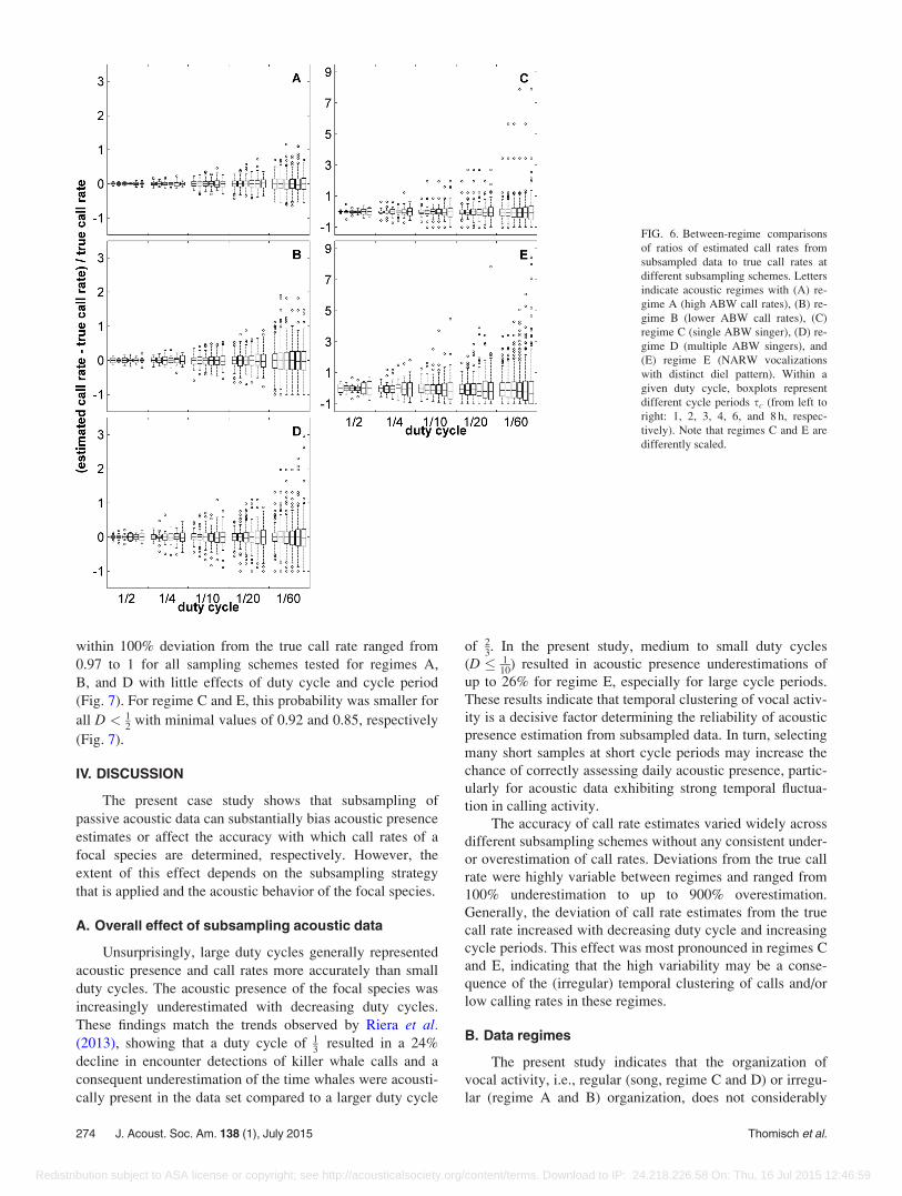
within 100% deviation from the true call rate ranged from

0.97 to 1 for all sampling schemes tested for regimes A,

B, and D with little effects of duty cycle and cycle period

(Fig. 7). For regime C and E, this probability was smaller for

all D < 12

with minimal values of 0.92 and 0.85, respectively

(Fig. 7).

IV. DISCUSSION

The present case study shows that subsampling of

passive acoustic data can substantially bias acoustic presence

estimates or affect the accuracy with which call rates of a

focal species are determined, respectively. However, the

extent of this effect depends on the subsampling strategy

that is applied and the acoustic behavior of the focal species.

A. Overall effect of subsampling acoustic data

Unsurprisingly, large duty cycles generally represented

acoustic presence and call rates more accurately than small

duty cycles. The acoustic presence of the focal species was

increasingly underestimated with decreasing duty cycles.

These findings match the trends observed by Riera et al.(2013), showing that a duty cycle of 1

3resulted in a 24%

decline in encounter detections of killer whale calls and a

consequent underestimation of the time whales were acousti-

cally present in the data set compared to a larger duty cycle

of 23. In the present study, medium to small duty cycles

(D � 110

) resulted in acoustic presence underestimations of

up to 26% for regime E, especially for large cycle periods.

These results indicate that temporal clustering of vocal activ-

ity is a decisive factor determining the reliability of acoustic

presence estimation from subsampled data. In turn, selecting

many short samples at short cycle periods may increase the

chance of correctly assessing daily acoustic presence, partic-

ularly for acoustic data exhibiting strong temporal fluctua-

tion in calling activity.

The accuracy of call rate estimates varied widely across

different subsampling schemes without any consistent under-

or overestimation of call rates. Deviations from the true call

rate were highly variable between regimes and ranged from

100% underestimation to up to 900% overestimation.

Generally, the deviation of call rate estimates from the true

call rate increased with decreasing duty cycle and increasing

cycle periods. This effect was most pronounced in regimes C

and E, indicating that the high variability may be a conse-

quence of the (irregular) temporal clustering of calls and/or

low calling rates in these regimes.

B. Data regimes

The present study indicates that the organization of

vocal activity, i.e., regular (song, regime C and D) or irregu-

lar (regime A and B) organization, does not considerably

FIG. 6. Between-regime comparisons

of ratios of estimated call rates from

subsampled data to true call rates at

different subsampling schemes. Letters

indicate acoustic regimes with (A) re-

gime A (high ABW call rates), (B) re-

gime B (lower ABW call rates), (C)

regime C (single ABW singer), (D) re-

gime D (multiple ABW singers), and

(E) regime E (NARW vocalizations

with distinct diel pattern). Within a

given duty cycle, boxplots represent

different cycle periods sc (from left to

right: 1, 2, 3, 4, 6, and 8 h, respec-

tively). Note that regimes C and E are

differently scaled.



impact the effects of subsampling. Instead, the calling activ-

ity level and potential temporal clustering of the focal spe-

cies’ vocal behavior determine the accuracy with which

subsampled data can represent the actual patterns in acoustic

behavior. Generally, species with high vocalization rates that

call throughout the day are more likely to be detected even

with small duty cycles compared to irregularly and/or rarely

calling species (Miksis-Olds et al., 2010). This is also

reflected in differences in the accuracies of call rate esti-

mates when regime pairs A and B as well as C and D are

compared; both basically exhibit the same temporal structure

but differ in the frequency of occurrence of calls, showing

the more calls, the higher the accuracy of call rate estimates.

Highest deviations between estimated and true call rates

were observed in regime E, representing vocal behavior with

a comparatively low vocalization rate and a distinct diel

pattern.

In the context of using passive acoustic data for density

estimation of calling animals, highly accurate call rate esti-

mates and/or knowledge on the potential uncertainty of these

estimates is crucial, as call rate linearly enters the density

estimates (Marques et al., 2013). Under subsampling, most

reliable results may be obtained by employing a subsampling

strategy that collects short samples at short cycle periods.

This will positively affect the accuracy with which cue rates

can be assessed as more of the natural variability can be cov-

ered by the sampling scheme.

However, subsampling acoustic recordings is not suita-

ble for species vocalizing rarely or to reliably capture unpre-

dictable temporal clusters of acoustic activity, for example,

when the species of interest passes the recorder’s acoustic

range only sporadically. Existing knowledge on the fre-

quency and timing of occurrences of temporal clusters in

vocal activity may aid the choice of a subsampling scheme,

provided that the patterns in vocal behavior of the focal spe-

cies are sufficiently well understood.

C. Subsampling strategies

Before deciding on a subsampling strategy, several

aspects concerning the research goal need consideration,

such as: What is the main purpose of the recording? What is

the temporal scale relevant to the investigation (e.g., is col-

lecting multi-year data worth the cost of subsampling to

cover the entire deployment period)? What knowledge on

acoustic behavior of the focal species is already available,

and is this representative for the study area and/or recording

season?

Single species studies, for example, investigating acous-

tic animal density in a given area, might benefit from adjust-

ing the recording parameters as much as possible to the

target species. When data storage is the limiting factor, stud-

ies investigating low-frequency baleen whale species may

decide to lower the sample rate to the minimum required to

FIG. 7. Between-regime comparisons of probabilities to estimate call rates from subsampled data within a specified range X [with X being 10% (upper panel),

50% (middle panel), and 100% (lower panel), respectively] of the true call rate at different subsampling schemes. Regimes A–E (indicated by different colors)

represent different vocal characteristics of the focal species as given in Fig. 6. Within a given duty cycle, markers indicate different cycle periods sc (from left

to right: 1, 2, 3, 4, 6, and 8 h, respectively).



capture only the calls of interest to maximize the time span

over which acoustic data can be collected. Alternatively,

adaptive subsampling may be considered to selectively cap-

ture only the events or species of interest throughout the

entire period, although this method is not appropriate to re-

cord rarely calling species or short events (e.g., Miksis-Olds

et al., 2010; Sousa-Lima et al., 2013). Furthermore, pilot

studies during which continuous records are collected in or

near the area of interest or information from previous inves-

tigations may provide a basis to decide on if and/or which

duty cycles are suitable to reliably capture the vocalizations

of interest. Recording in a Matryoshka mode may provide a

solution to collect detailed “snapshots” that can be used to,

for example, gauge acoustic animal densities during specific

parts of the year. Matryoshka mode, referring to the Russian

nested dolls, employs continuous or large duty cycles that

are again set to cycle over a larger time scale.

For studies aiming to explore acoustic biodiversity or

soundscape ecology in an area for which no acoustic records

exist yet, it may be inevitable to collect continuous records

given that principally all events are of interest. By, for exam-

ple, continuously collecting a week of data each month, a

relatively reliable overview of the event types and species

that are (substantially) acoustically present in the vicinity of

the recorder may be gained throughout the entire recording

time span, depending on the storage and battery capacity of

the recording instrument. To reliably capture transiting spe-

cies or species that frequent the region only sporadically,

truly continuous records are the only possibility to collect

reliable information. When logistically and financially possi-

ble, multiple recorders programmed to record subsequently

after the previous one has stopped may allow covering

the entire period that the devices are in the water with

(near-)continuous acoustic data.

Alongside maximizing the probability of capturing the

species of interest, requirements on the acoustic data to

answer specific research questions should also be taken

into account. For example, humpback whale (Megapteranovaeangliae) acoustic presence may be reliably estimated

from short samples at short cycle periods data with relatively

small duty cycles, however assessing the number of singers

and in-detail analyses of song structure require substantially

longer samples.

The decision on a certain subsampling strategy is often

not primarily (or not at all) driven by biological parameters

or considerations. The only recording parameter that in most

cases is adapted to meet the specific research objectives is the

sample rate, which (when too low) may result in missed call

events or species misidentification due to, for example, alias-

ing (Oswald et al., 2004). The fact that other vocal character-

istics of the focal species are not evaluated when deciding on

sampling strategies is in most cases not an active decision but

rather the result of lacking knowledge on the acoustic behav-

ior for many species (e.g., Mellinger et al., 2007). However,

informed decisions on subsampling strategies can only be

based on a solid understanding of vocal behavior for which,

ironically, a representative acoustic sampling strategy is

fundamental. If such information is not available, it may be

preferable to collect continuous samples of limited duration

across the year.

Technological developments may sooner or later allow

autonomous collection of continuous acoustic records over

long time scales with high sample rates, relaxing the need to

record in subsampling mode due to instrument limitations.

Nevertheless, these extensive data sets also need to be

analyzed and stored which are other aspects where subsam-

pling again may come into play. However, in contrast to sub-

sampled recordings, subsampled analyses allow evaluation

of the representativeness of the selected sampling strategy

by comparisons to the continuous data records, according to

the principle applied in the present case study.

V. CONCLUSION

The present case study demonstrates that subsampling

acoustic data might have substantial effects on the assess-

ment of acoustic presence and call rate, depending on the

vocal characteristics of the focal species. If subsampling at a

given duty cycle is mandatory due to logistic constraints,

data collection in many short listening periods is preferable.

Such sampling scheme results in many sampling cycles per

day and hence, enables optimal representation of potential

variability in the vocal behavior throughout the day and is

best suited for assessments of both acoustic presence and

call rate of the focal species.

Vocal characteristics as represented by different acous-

tic regimes in this study partly affected the accuracy of

acoustic presence and call rate estimates from subsampled

data. The organization of vocal activity (i.e., in terms of reg-

ular or irregular structure of vocalizations) did not markedly

affect the results from subsampled data. Contrastingly,

differences in vocalization rates had considerable impact on

acoustic presence and call rate estimates from subsampled

data, with accuracy improving with increasing call rates (in

the continuous data). Furthermore, temporal clustering of

vocal activity (i.e., diel vocalization pattern) considerably

decreased the accuracy with which acoustic presence and

call rates were assessed in the present study.

Subsampling during data collection may not be neces-

sary in studies on species vocalizing at low frequencies as

the sampling rate may be adjusted to a comparatively low

level and in turn, recording continuously during the entire

deployment period may be possible. However, subsampling

may increasingly become necessary when shifting the focus

towards species with high-frequency vocalizations as well as

in multi-species studies covering a broad frequency range to

investigate an area’s acoustic biodiversity or soundscape.

While technological advancements concerning power supply

and data storage capacities will likely allow acquisition of

large (near-)continuous data sets in the near future, human

screening of the data will in many cases still be necessary to

a certain degree, for example, for verification of automatic

detection outcomes, and in turn, may still require subsam-

pling of the total data to be manageable.

Polar oceans are areas where subsampling of acoustic

recordings occurs relatively frequently as a consequence of

the logistic difficulties of accessing the area. For many



species inhabiting the polar oceans, relatively little is known

on acoustic diversity, interactions, and acoustics-based ani-

mal densities, whereas gaining insights as to how climate-

induced ecosystem changes affect the species in these areas

is particularly crucial in the context of monitoring and

managing potential changes. Optimizing passive acoustic

data collection procedures in terms of sampling strategies

lies at the heart of improving the current status of knowledge

and providing fundamental information for future manage-

ment and conservation strategies.

ACKNOWLEDGMENTS

We thank Jean-Yves Royer for the sampling of the

SWAMS data collected for the Deflo-Hydro program. Many

thanks to Lars Kindermann for maintenance of the PALAOA

observatory, processing and providing the PALAOA data.

Stefanie Spiesecke, Elke Burkhardt, and Stefan Frickenhaus

have provided conceptual advice and insightful comments on

the present study. Special thanks to the logistics department

of the Alfred Wegener Institute for Polar and Marine

Research, Bremerhaven, Germany, Reederei F. Laeisz

GmbH, Rostock, Germany and FIELAX Services for Marine

Science and Technology GmbH, Bremerhaven, Germany and

the overwintering teams at Neumayer Station for their

contribution to setup and/or maintenance of PALAOA.

Boebel, O., Kindermann, L., Klinck, H., Bornemann, H., Pl€otz, J.,

Steinhage, D., Riedel, S., and Burkhardt, E. (2006). “Real-time underwater

sounds from the Southern Ocean,” EOS Trans. Am. Geophys. Union 87,

361.

Burtenshaw, J. C., Oleson, E. M., Hildebrand, J. A., McDonald, M. A.,

Andrew, R. K., Howe, B. M., and Mercer, J. A. (2004). “Acoustic and sat-

ellite remote sensing of blue whale seasonality and habitat in the

Northeast Pacific,” Deep Sea Res. (II Top. Stud. Oceanogr.) 51, 967–986.

Clark, C. W. (1982). “The acoustic repertoire of the Southern right whale, a

quantitative analysis,” Anim. Behav. 30, 1060–1071.

Di Iorio, L., and Clark, C. W. (2010). “Exposure to seismic survey alters

blue whale acoustic communication,” Biol. Lett. 6, 51–54.

Figueroa, H., and Robbins, K. (2008). “XBAT: An open-source extensible

platform for bioacoustic research and monitoring,” in ComputationalBioacoustics for Assessing Biodiversity, edited by K.-H. Frommolt, R.

Bardeli, and M. Clausen (Bundesamt f€ur Naturschutz, Bonn), pp.

143–155.

Gedamke, J., Gales, N., Hildebrand, J., and Wiggins, S. (2007). “Seasonal

occurrence of low frequency whale vocalisations across eastern Antarctic

and southern Australian waters, February 2004 to February 2007,” SC/59/

SH57, presented to the IWC Scientific Committee, 2007, Anchorage, AK,

pp. 11.

Harris, D., Matias, L., Thomas, L., Harwood, J., and Geissler, W. H. (2013).

“Applying distance sampling to fin whale calls recorded by single seismic

instruments in the northeast Atlantic,” J. Acoust. Soc. Am. 134,

3522–3535.

Kindermann, L., Boebel, O., Bornemann, H., Burkhardt, E., Klinck, H., van

Opzeeland, I., Pl€otz, J., and Seibert, A.-M. (2008). “A perennial acoustic

observatory in the Antarctic Ocean,” in Computational Bioacoustics forAssessing Biodiversity, edited by K.-H. Frommolt, R. Bardeli, and M.

Clausen (Bundesamt f€ur Naturschutz, Bonn), pp. 15–28.

K€usel, E. T., Mellinger, D. K., Thomas, L., Marques, T. A., Moretti, D., and

Ward, J. (2011). “Cetacean population density estimation from single

fixed sensors using passive acoustics,” J. Acoust. Soc. Am. 129,

3610–3622.

Ljungblad, D. K., Clark, C. W., and Shimada, H. (1998). “A comparison of

sounds attributed to pygmy blue whales (Balaenoptera musculus brevi-cauda) recorded south of the Madagascar Plateau and those attributed to

‘true’ blue whales (Balaenoptera musculus) recorded off Antarctica,” Rep.

Intl. Whal. Comm. 48, 439–442.

Marques, T. A., Munger, L., Thomas, L., Wiggins, S., and Hildebrand, J. A.

(2011). “Estimating North Pacific right whale Eubalaena japonica density

using passive acoustic cue counting,” Endanger. Species Res. 13, 163–172.

Marques, T. A., Thomas, L., Martin, S. W., Mellinger, D. K., Ward, J. A.,

Moretti, D. J., Harris, D., and Tyack, P. L. (2013). “Estimating animal

population density using passive acoustics,” Biol. Rev. 88, 287–309.

Matthews, L. P., McCordic, J. A., and Parks, S. E. (2014). “Remote acoustic

monitoring of North Atlantic right whales (Eubalaena glacialis) reveals

seasonal and diel variations in acoustic behavior,” PLoS One 9, e91367.

McDonald, M. A., Hildebrand, J. A., and Webb, S. C. (1995). “Blue and fin

whales observed on a seafloor array in the Northeast Pacific,” J. Acoust.

Soc. Am. 98, 712–721.

Melc�on, M. L., Cummins, A. J., Kerosky, S. M., Roche, L. K., Wiggins, S.

M., and Hildebrand, J. A. (2012). “Blue whales respond to anthropogenic

noise,” PLoS One 7, e32681.

Mellinger, D. K., Stafford, K. M., Moore, S., Dziak, R. P., and Matsumoto,

H. (2007). “An overview of fixed passive acoustic observation methods

for cetaceans,” Oceanography 20, 36–45.

Miksis-Olds, J. L., Nystuen, J. A., and Parks, S. E. (2010). “Detecting ma-

rine mammals with an adaptive sub-sampling recorder in the Bering Sea,”

Appl. Acoust. 71, 1087–1092.

Monnahan, C. C., Branch, T. A., Stafford, K. M., Ivashchenko, Y. V., and

Oleson, E. M. (2014). “Estimating historical eastern north pacific blue

whale catches using spatial calling patterns,” PLoS One 9, e98974.

Mussoline, S. E., Risch, D., Hatch, L. T., Weinrich, M. T., Wiley, D. N.,

Thompson, M. A., Corkeron, P. J., and Van Parijs, S. M. (2012).

“Seasonal and diel variation in North Atlantic right whale up-calls:

Implications for management and conservation in the northwestern

Atlantic Ocean,” Endanger. Species Res. 17, 17–26.

Oleson, E. M., Wiggins, S. M., and Hildebrand, J. A. (2007). “Temporal

separation of blue whale call types on a southern California feeding

ground,” Anim. Behav. 74, 881–894.

Oswald, J. N., Rankin, S., and Barlow, J. (2004). “The effect of recording

and analysis bandwidth on acoustic identification of delphinid species,”

J. Acoust. Soc. Am. 116, 3178–3185.

Parks, S. E., and Clark, C. (2007). “Acoustic communication: Social sounds

and the potential impacts of noise,” in The Urban Whale: North AtlanticRight Whales at the Crossroads, edited by S. D. Kraus and R. M. Rolland

(Harvard University Press, Cambridge, MA), pp. 310–333.

Rankin, S., Ljungblad, D., Clark, C., and Kato, H. (2005). “Vocalisations of

Antarctic blue whales, Balaenoptera musculus intermedia, recorded dur-

ing the 2001/2002 and 2002/2003 IWC/SOWER circumpolar cruises,

Area V, Antarctica,” J. Cetacean Res. Manage 7, 13–20.

Rettig, S., Boebel, O., Menze, S., Kindermann, L., Thomisch, K., and van

Opzeeland, I. (2013). “Local to basin scale arrays for passive acoustic

monitoring in the Atlantic sector of the Southern Ocean,” in InternationalConference and Exhibition on Underwater Acoustics, edited by J.

Papadakis, and L. Bjorno, Corfu Island, Greece.

Riera, A., Ford, J. K., and Chapman, N. R. (2013). “Effects of different anal-

ysis techniques and recording duty cycles on passive acoustic monitoring

of killer whales,” J. Acoust. Soc. Am. 134, 2393–2404.

Samaran, F., Adam, O., and Guinet, C. (2010). “Discovery of a mid-latitude

sympatric area for two southern hemisphere blue whale subspecies,”

Endanger. Species Res. 12, 157–165.

Samaran, F., Stafford, K. M., Branch, T. A., Gedamke, J., Royer, J.-Y., Dziak,

R. P., and Guinet, C. (2013). “Seasonal and geographic variation of southern

blue whale subspecies in the Indian Ocean,” PLoS One 8, e71561.�Sirovic, A., and Hildebrand, J. A. (2011). “Using passive acoustics to model

blue whale habitat off the Western Antarctic Peninsula,” Deep Sea Res. (II

Top. Stud. Oceanogr.) 58, 1719–1728.�Sirovic, A., Hildebrand, J. A., and Wiggins, S. M. (2007). “Blue and fin

whale call source levels and propagation range in the Southern Ocean,”

J. Acoust. Soc. Am. 122, 1208–1215.�Sirovic, A., Hildebrand, J. A., Wiggins, S. M., McDonald, M. A., Moore, S.

E., and Thiele, D. (2004). “Seasonality of blue and fin whale calls and the

influence of sea ice in the Western Antarctic Peninsula,” Deep Sea Res. (I

Oceanogr. Res. Pap.) 51, 2327–2344.�Sirovic, A., Hildebrand, J. A., Wiggins, S. M., and Thiele, D. (2009). “Blue

and fin whale acoustic presence around Antarctica during 2003 and 2004,”

Mar. Mamm. Sci. 25, 125–136.

Sousa-Lima, R. S., Norris, T. F., Oswald, J. N., and Fernandes, D. P. (2013).

“A review and inventory of fixed autonomous recorders for passive acous-

tic monitoring of marine mammals,” Aquat. Mamm. 39, 23–53.



http://dx.doi.org/10.1029/2006EO360002

http://dx.doi.org/10.1016/j.dsr2.2004.06.020

http://dx.doi.org/10.1016/S0003-3472(82)80196-6

http://dx.doi.org/10.1098/rsbl.2009.0651

http://dx.doi.org/10.1121/1.4821207

http://dx.doi.org/10.1121/1.3583504

http://dx.doi.org/10.3354/esr00325

http://dx.doi.org/10.1111/brv.12001

http://dx.doi.org/10.1371/journal.pone.0091367

http://dx.doi.org/10.1121/1.413565

http://dx.doi.org/10.1121/1.413565


http://dx.doi.org/10.5670/oceanog.2007.03

http://dx.doi.org/10.1016/j.apacoust.2010.05.010



http://dx.doi.org/10.1016/j.anbehav.2007.01.022

http://dx.doi.org/10.1121/1.1804635

http://dx.doi.org/10.1121/1.4816552





http://dx.doi.org/10.1121/1.2749452



http://dx.doi.org/10.1111/j.1748-7692.2008.00239.x

Stafford, K. M., Bohnenstiehl, D. R., Tolstoy, M., Chapp, E., Mellinger, D.

K., and Moore, S. E. (2004). “Antarctic-type blue whale calls recorded at

low latitudes in the Indian and eastern Pacific Oceans,” Deep Sea Res. (I

Oceanogr. Res. Pap.) 51, 1337–1346.

Stafford, K. M., Moore, S. E., Berchok, C. L., Wiig, Ø., Lydersen, C.,

Hansen, E., Kalmbach, D., and Kovacs, K. M. (2012). “Spitsbergen’s

endangered bowhead whales sing through the polar night,” Endanger.

Species Res. 18, 95–103.

Stafford, K. M., Moore, S. E., and Fox, C. G. (2005). “Diel variation in blue

whale calls recorded in the eastern tropical Pacific,” Anim. Behav. 69, 951–958.

Van Opzeeland, I. (2010). “Acoustic ecology of marine mammals in polar

oceans,” Berichte zur Polar-und Meeresforschung (Reports on Polar and

Marine Research), Vol. 619, 332 pp.

Van Opzeeland, I., Van Parijs, S., Bornemann, H., Frickenhaus, S.,

Kindermann, L., Klinck, H., Pl€otz, J., and Boebel, O. (2010). “Acoustic

ecology of Antarctic pinnipeds,” Mar. Ecol. Prog. Ser. 414, 267–291.

Van Opzeeland, I., Van Parijs, S., Kindermann, L., Burkhardt, E., and

Boebel, O. (2013). “Calling in the cold: Pervasive acoustic presence of

humpback whales (Megaptera novaeangliae) in Antarctic coastal waters,”

PLoS One 8, e73007.

Van Parijs, S. M., Clark, C. W., Sousa-Lima, R. S., Parks, S. E., Rankin,

S., Risch, D., and van Opzeeland, I. C. (2009). “Management and

research applications of real-time and archival passive acoustic sensors

over varying temporal and spatial scales,” Mar. Ecol. Prog. Ser. 395,

21–36.

Ward, J. A., Thomas, L., Jarvis, S., Dimarzio, N., Moretti, D., Marques, T.

A., Dunn, C., Claridge, D., Hartvig, E., and Tyack, P. (2012). “Passive

acoustic density estimation of sperm whales in the Tongue of the Ocean,

Bahamas,” Mar. Mamm. Sci. 28, E444–E455.

Wiggins, S. M., Oleson, E. M., McDonald, M. A., and Hildebrand, J. A.

(2005). “Blue whale (Balaenoptera musculus) diel call patterns offshore

of Southern California,” Aquat. Mamm. 31, 161–168.



http://dx.doi.org/10.1016/j.dsr.2004.05.007

http://dx.doi.org/10.1016/j.dsr.2004.05.007



http://dx.doi.org/10.1016/j.anbehav.2004.06.025

http://dx.doi.org/10.3354/meps08683


http://dx.doi.org/10.3354/meps08123

http://dx.doi.org/10.1111/j.1748-7692.2011.00560.x

http://dx.doi.org/10.1578/AM.31.2.2005.161

Effects of subsampling of passive acoustic recordings on ... et al... · Effects of subsampling of...

Documents

Transcript of Effects of subsampling of passive acoustic recordings on ... et al... · Effects of subsampling of...