1

Effects of Genetic and Environmental Factors on Trait Network Predictions from

Quantitative Trait Locus Data

David L. Remington

University of North Carolina at Greensboro, Greensboro, North Carolina 27402

Genetics: Published Articles Ahead of Print, published on January 12, 2009 as 10.1534/genetics.108.092668

2

Running head: Factors affecting QTL functional prediction

Keywords: quantitative trait locus, structural equation model, functional prediction, trait

network, common environment

Corresponding author: David L. Remington, Department of Biology, 312 Eberhart Bldg.,

University of North Carolina at Greensboro, P.O. Box 26170, Greensboro, NC 27402-6170. tel:

336-334-4967. fax: 336-334-5839. e-mail: dlreming@uncg.edu

3

ABSTRACT

The use of high-throughput genomic techniques to map gene expression quantitative trait

loci (eQTLs) has spurred the development of path analysis approaches for predicting functional

networks linking genes and natural trait variation. The goal of this study was to test whether

potentially confounding factors, including effects of common environment and genes not

included in path models, affect predictions of cause-effect relationships among traits generated

by QTL path analyses. Structural equation modeling (SEM) was used to test simple QTL-trait

networks under different regulatory scenarios involving direct and indirect effects. SEM

identified the correct models under simple scenarios, but when common environmental effects

were simulated in conjunction with direct QTL effects on traits, they were poorly distinguished

from indirect effects, leading to false support for indirect models. Application of SEM to

loblolly pine QTL data provided support for biologically plausible a priori hypotheses of QTL

mechanisms affecting height and diameter growth. However, some biologically implausible

models were also well-supported. The results emphasize the need to include any available

functional information, including predictions for genetic and environmental correlations, to

develop plausible models if biologically useful trait network predictions are to be made.

4

The emergence of genome technologies provides unprecedented opportunities to dissect

the networks of gene regulation, expression, functions, and interactions by which genes affect

phenotypes. The field of systems biology arising from these opportunities has been devoted

primarily to understanding constitutive processes through investigations and modeling of

phenotypic effects of knockout mutants, but recent interests have expanded into understanding

how natural genetic variation affects phenotypic variability (BENFEY and MITCHELL-OLDS 2008;

FEDER and MITCHELL-OLDS 2003; KEURENTJES et al. 2008; KOONIN and WOLF 2008). Genetic

mapping of quantitative trait loci (QTLs) in segregating families has become a key tool for

uncovering the genetic architecture of natural trait variation and ultimately identifying the

underlying genes over the last two decades (MACKAY 2001; MACKAY 2004). However, the use

of high-throughput techniques has expanded the definition of “quantitative trait” to encompass

transcript levels assayed on a genome-wide scale, leading to expression QTL (eQTL) mapping

(BREM et al. 2002; KEURENTJES et al. 2007; SCHADT et al. 2005), and similar approaches are

being used to map QTLs associated with metabolomic variation (KEURENTJES et al. 2006; LISEC

et al. 2008).

Interest in incorporating eQTL data into a systems biology framework has spawned the

development of new analytical approaches for predicting functional networks linking genes and

traits using multiple-trait QTL data. Basic methods for combined analysis of traditional

multiple-trait QTLs, such as mapping QTLs for eigenvectors defined by principal components

analysis (PCA; BREWER et al. 2007; LANGLADE et al. 2005) and multiple-trait QTL analysis

(HALL et al. 2006; JIANG and ZENG 1995; RAUH et al. 2002), may be useful for detecting

pleiotropic (or closely linked) QTLs and providing insights on the nature of multiple-trait QTL

effects, but yield little information for causal inference. One proposed method for identifying

5

key regulators of gene expression variation uses average expression levels of gene regulatory

networks identified a priori as composite traits for eQTL analysis (KLIEBENSTEIN et al. 2006).

In another approach, expression patterns of genes located within eQTL regions shared among

genes in known pathways are compared to those of the genes in the pathway to identify likely

pathway regulators (KEURENTJES et al. 2007).

In contrast with the above approaches, DOSS et al. (2005) suggested using patterns of

overall vs. residual correlations of gene expression in eQTL studies, which differ among tightly

linked genes for pairs with shared vs. independent regulatory mechanisms, in combination with

path analysis to make causative predictions about gene regulation. Inference methods based on

this reasoning have been proposed for de novo prediction of causal relationships in gene

regulatory pathways (LIU et al. 2008; ZHU et al. 2004), between gene regulation processes and

disease (SCHADT et al. 2005), and among sets of functionally related complex morphological and

metabolic phenotypes (LI et al. 2006). Various models of network regulatory structure, in which

sets of QTLs control variation in multiple traits directly or indirectly through cause-effect

relationships, are tested with genetic marker and trait data to identify the models best supported

by the data. Statistical approaches include Bayesian networks (ZHU et al. 2004), likelihood

methods to evaluate conditional trait correlations for their support under alternative regulatory

model configurations (NETO et al. 2008; SCHADT et al. 2005), and structural equation modeling

to compare the fit of different regulatory path models to the multiple-trait covariance structure

(LI et al. 2006; LIU et al. 2008). These techniques use information from residual trait

correlations that is normally neglected in conventional QTL analysis, with the exception of some

multiple-trait QTL analysis techniques (JIANG and ZENG 1995) where it is used to increase the

power to detect joint QTLs but not for functional prediction.

6

Structural equation modeling (SEM) is well-suited to causal network prediction because

it can accommodate a large variety of model structures including feedback relationships (LIU et

al. 2008) and is adaptable to various modes of exploratory and confirmatory analyses of

biological models (LI et al. 2006; LIU et al. 2008; STEIN et al. 2003; TONSOR and SCHEINER

2007). Moreover, SEM is supported by software packages such as SAS/STAT (SAS INSTITUTE

INC. 2002) and AMOS (AMOS DEVELOPMENT CORPORATION 2006). Path analysis has long been

recognized as potentially valuable but probably underutilized tool for testing causative rather

than merely correlative relationships in quantitative genetic data (LYNCH and WALSH 1998;

WRIGHT 1921). Nevertheless, some important issues must be considered in evaluating the

reliability of SEM and other path analysis methodologies for inferring trait networks from QTL

data. For one thing, cause-effect relationships between traits, environmental effects, and effects

of other QTLs can all generate within-genotype trait correlations (DOSS et al. 2005; SCHADT et

al. 2005; STEIN et al. 2003). Can path analysis correctly distinguish these potentially

confounding effects? Secondly, how valid are the results of path analysis for exploring the

likelihood of different model structures (i.e. different directions of cause-effect relationships

among traits) rather than merely testing for the presence of particular connections within an

established structure or estimating path coefficients for a particular model? Third, the true

regulatory networks shaping patterns of trait variation may be much more complex than the

tested models, including feedback loops or unobserved traits and QTLs (LIU et al. 2008; SCHADT

et al. 2005). Under these circumstances, will poor support for overly simple models provide

reliable clues to the existence of a more complex network structure?

The goal of this study was to test the causal inferences from structural equation models

under a set of relatively simple QTL regulatory scenarios. Specifically, I wanted to test whether

7

models could correctly distinguish direct vs. indirect mechanisms of QTL effects on a pair of

traits, and test the effects of incomplete identification of QTLs, common environmental effects,

and direct regulation of unobserved traits on model predictions. To do this, I simulated multiple

QTL data sets using a backcross design involving three QTLs jointly affecting two traits in

various direct and indirect modes of action. SEMs representing different models were tested for

their capability to distinguish the correct functional scenario from incorrect scenarios in each

case. For the sake of consistent comparisons, similar locations for each QTL and similar sets of

effect sizes on the observed traits were simulated under all of the initial scenarios, a constraint

that was later relaxed. Finally, I used SEM to evaluate data from a loblolly pine (Pinus taeda L.)

QTL study of diameter and height growth, for which biologically reasonable predictions could be

made about models of joint genetic effects on the set of traits.

MATERIALS AND METHODS

QTL simulations and detection: All data sets were initially simulated using QTL

Cartographer version 1.17 (BASTEN et al. 1994; BASTEN et al. 2004) and modified as needed to

incorporate indirect QTL effects. The simulated genome using the Rmap routine consisted of

five chromosomes, each with 8 markers spaced 15 cM apart starting at position 0 cM, generated

using the Kosambi map function. Three QTLs were simulated using Rqtl at the following

locations: chromosome 1, 50 cM (Q1); chromosome 2, 40 cM (Q2); and chromosome 3, 60 cM

(Q3). Thus, the first two simulated QTLs were in intervals between markers and the third was at

a marker position. Environmental variance was set to keep the total phenotypic variance close to

1.0 so all effect sizes would be approximately in phenotypic standard deviation units. Effects of

8

all QTLs were strictly additive, with simulated allele substitution effects (a) after all

modifications on traits T1 and T2, respectively, of 0.7 and 0.5 for Q1, and 0.5 and 0.35 for Q2

and Q3. Thus, a for each QTL was uniformly greater on T1 than on T2 by a factor of

approximately 2 and the simulated variance explained by each QTL for T1 was very close to

double that for T2. Backcross families of 500 progeny segregating for the genetic markers and

three QTLs in the two traits were simulated in QTL Cartographer using Rcross.

Direct-effects scenario: Under a scenario of direct effects, the simulated QTLs directly

and independently affect both traits (Figure 1a). All marker and trait data were directly

simulated in QTL Cartographer as described above.

Indirect-effects scenario: Under the indirect (or cause-effect) scenario, the simulated

QTLs directly affect only trait 1, which in turn affects trait 2 (Figure 1b). Only the data for t1

was simulated in QTL Cartographer with the effect sizes as described above for the basic model.

Data for t2 were simulated using the equation:

iii ztt 22

122

2 += , (1)

where t1i and t2i are the values for T1 and T2, respectively, in progeny i, and zi is a standard

normal random variate generated using the RANNOR command in SAS version 9 (SAS

INSTITUTE INC. 2002). Thus, half the variance in T2 is explained by the value of T1, yielding

expected substitution effects for Q1, Q2, and Q3 of approximately 0.5, 0.35, and 0.35,

respectively, in T2, similar to the effect sizes under the direct effects model. A new marker-trait

input file was then created for Rcross that included the simulated values for both traits.

Latent-direct scenario: In this scenario, the three QTLs are assumed to have direct

effects on an unobserved trait T0, which in turn has independent direct effects on T1 and T2

(Figure 1c). Progeny values for T0 were simulated in Rcross using substitution effects of 1.0,

9

0.7, and 0.7 for the three QTLs. Progeny values for T1 and T2 were then simulated using the

equations:

iii ztt 122

022

1 += , (2a)

and

iii ztt 223

021

2 += , (2b)

with T0 explaining half of the variance in T1 and one quarter of the variance in T2, where z1i and

z2i are standard normal variates. This resulted in substitution effects for the three QTLs on the

two traits that were similar to those described above for the base model. The generated values

for t1 and t2 were then used as input into Rcross.

Direct-effects common-environment scenarios: In these scenarios, the simulated QTLs

directly and independently affected the two traits in similar fashion to the direct effects model,

but a common environmental effect on the two traits was included (Figure 1d). To generate

simulated data sets under this scenario, two traits T1* and T2* were first simulated using Rqtl and

Rcross, with Q1, Q2, and Q3 having substitution effects of 1.0, 0.7, and 0.7, respectively, on T1*

and 0.7, 0.5, and 0.5 on T2*. Three vectors of standard normal variates, zC, z1, and z2, were then

generated to represent common, T1-specific, and T2-specific environmental effects, respectively.

Progeny values for T1 and T2 were then generated using the equations:

iCiii czbztt 1*12

21 ++= , (3a)

and

iCiii czbztt 2*22

22 ++= . (3b)

Values of b and c were chosen so that b2 + c2 = 0.5, and were varied in different simulated data

sets to adjust the strength of the common environmental effect. Values of 22=b and c = 0 were

10

used to simulate strong environmental correlation, and 15.0=b and 35.0=c were used to

generate a weaker environmental correlation. The resulting substitution effects of QTLs on the

two traits were thus similar to those of the base model. The values for T1 and T2 were then

substituted for the original T1* and T2* values as input into QTL Cartographer.

Heterogeneous-effects common-environment scenarios: These scenarios were similar to

the direct-effects common-environment scenarios and data were generated using the same

approach, except that the assumption of a homogeneous ratio of relative QTL effects on the two

traits was relaxed (Figure 1e). Values for T1* and T2* were changed to result in substitution

effects for Q1, Q2, and Q3 of 0.7, 0.5, and 0.3 for T1, and 0.5, 0.5, and 0.5 for T2. Both strong

and weak environmental correlations were simulated in different data sets.

F2 direct-effects scenario: A model with direct and independent effects on the two traits

was also used to simulate an F2 family of 500 progeny. QTL locations and additive substitution

effects on the two traits were identical to the basic model described above, and a dominance

effect was also included such that the simulated d/a ratio for both traits was 22 for Q1, 1.0 for

Q2, and 0 for Q3.

QTL detection and structural equation modeling: QTL effects and locations were

estimated by maximum-likelihood composite interval mapping in QTL Cartographer, using

model 6 in Zmapqtl. Prior to running Zmapqtl, background markers were fit using forward plus

backward stepwise regression using a p-value threshold of 0.05 in SRmapqtl to control for

background effects including those of other QTLs when conducting the QTL scans. In Zmapqtl,

a 2 cM walking speed was used to scan the genome for QTL effects, a window size of 10 cM

around each tested position was used to control for QTL effects outside the current marker

interval, and up to 5 of the markers selected in SRmapqtl were used to control for background

11

effects. For backcross data sets, an empirical genome-wide α = 0.05 likelihood ratio test statistic

threshold of 11.28 was estimated from 1000 permutations of simulated data set 1 for the direct

effects scenario. For F2 data sets, an empirical threshold of 14.37 was similarly estimated from

permutation tests of one of the two F2 simulations. Finally, multiple-trait composite interval

mapping was done using model 6 in JZmapqtl to estimate joint QTL effects on the two traits.

The positions with the peak multiple-trait likelihood ratios when comparing the full and reduced

(a = 0) models were used as the QTL locations in the subsequent SEM analysis in place of the

“true” simulated locations. If the detected multiple-trait likelihood peaks were more than 3 cM

outside the range defined by the single-trait likelihood peaks identified using Zmapqtl, a location

closer to the range of the detected single-trait peaks was chosen to represent the QTL.

“Virtual markers” were generated for the likelihood ratio peak locations of each detected

QTL. For backcross progeny sets, the virtual marker score was the probability of inheriting a

donor parent allele from the heterozygous parent, given the flanking marker genotypes (coded as

1 for a heterozygote and 0 for a recurrent parent homozygote) and recombination frequencies

with the respective markers. For F2 progeny, additive genotypic coefficients at flanking markers

were scored as 1, 0, and -1 for parent 1 homozygotes, heterozygotes, and parent 2 homozygotes,

respectively. Dominance coefficients were scored as 0.5 and -0.5 for heterozygotes and

homozygotes, respectively. The additive and dominance scores for each virtual marker were

calculated as the expected values of the additive and dominance genotypic coefficients at the

estimated QTL position, given the flanking marker scores and recombination frequencies with

each marker. The MultiRegress module in QTL Cartographer was used to calculate the additive

and dominance scores for the F2 datasets

12

SEM was conducted using PROC CALIS in SAS version 9 (SAS INSTITUTE INC. 2002).

SEMs were implemented by solving a set of linear equations for each tested model using

maximum-likelihood estimation, with each equation describing a trait value (an endogenous

variable) as a linear function of variables directly “upstream”, which could be virtual marker

scores at QTL positions and/or another trait. In F2 designs, additive and dominance scores at

each virtual marker were included as separate variables. Virtual markers for all QTLs significant

at the empirical threshold for at least one of the two traits were included as variables in the SEM.

All simulated QTLs were detected with genome-wide significance for at least one, and generally

both, traits. In all cases in which a simulated QTL lacked genome-wide significance for a trait, a

likelihood ratio peak with at least comparisonwise significance was present. In several simulated

data sets, significant effects were also detected at loci that did not correspond to simulated QTL

locations, and these were also included in the models. The coefficients of the virtual marker

scores in the linear equations represent the maximum-likelihood estimates of direct QTL effects

on the traits. This approach differs from the mixture model maximum-likelihood estimation used

for interval mapping in QTL Cartographer. However, in models in which the only explanatory

variables were direct QTL effects on the observed traits, the estimated QTL effects from SEM

were very similar to those obtained with QTL Cartographer. When common environmental

effects were included in models, they were incorporated either as unobserved variables (known

as latent variables) affecting multiple traits or as a covariance between the error terms for the

traits, with both approaches producing the same results. The SEM methodology described above

was implemented in PROC CALIS by using Lineqs statements.

Analyses of all data sets included: (a) a full model with direct effects of all three QTLs

on both T1 and T2 and indirect effects of T1 on T2 (Fig. 1f); (b) a direct-effects model

13

corresponding to Figure 1a; (c) an indirect-effects model corresponding to Figure 1b; and (d) a

reversed indirect-effects model, corresponding to Figure 1b but with T2 downstream of T1. The

full model under both backcross and F2 scenarios could not be tested because it was fully

specified (i.e. had zero degrees of freedom), and thus the solutions resulted in a perfect fit to the

covariance structure of the marker-trait data (see also NETO et al. 2008). Alternative fully-

specified models with the same sets of observed (manifest) variables but different path structures

also have a statistically equivalent perfect fit to the data. Including the full model in the

analyses, however, provided unique estimates of the relative contributions of the direct and

indirect paths to the values of T2, given the model structure. A model corresponding to the

direct-effects common-environment scenario (Figure 1d) could not be tested under the simulated

conditions. This model has no degrees of freedom if all QTLs are included as effects for both

traits, and thus the maximum-likelihood solutions perfectly fit the data as in the full model.

Models corresponding to the latent direct scenario (Figure 1c, with the unobserved T0 included

in the model as a latent variable) also could not be validly tested. Due to the path structure in

which T0 is directly connected to all explanatory QTLs and observed traits, the latent variable

can be fit optimally to be highly correlated to the upstream trait in an indirect scenario or to

characterize the correlated QTL effects on the two traits in a direct scenario. Consequently, a

latent direct model fit the data better than both the direct and indirect models under all of the

simulated scenarios and is uninformative about the true model.

Structural equation models were evaluated and compared using three criteria. (1) The

likelihood ratio (LR) test statistic (LRT) is -2 times the log likelihood ratio for the data under the

tested model vs. a fully-specified model. All tested models are nested within a fully-specified

model (either the full model described above or a statistically equivalent model with a different

14

path structure), so the LR test statistic has an asymptotic χ2 distribution based on the number of

degrees of freedom in the tested model. A significant p-value (p < 0.05) represents a failure of

the tested model to explain the covariance structure of the data fully (i.e. insufficiency of the

model), and insignificant p-values identify models that adequately fit the data (MITCHELL 1992).

(2) Standard and adjusted goodness-of-fit indices (GFI and AGFI, respectively) estimate model

fit based on the residual errors, with the latter adjusted for degrees of freedom. Thus, GFI may

be considered analogous to the R2 in a linear model and AGFI analogous to an adjusted R2.

While both measures should produce values between 0 and 1, poorly-fitting models with small

degrees of freedom may result in negative AGFI (PROC CALIS documentation in SAS

INSTITUTE INC. 2002). (3) Akaike’s Information Criterion (AIC; AKAIKE 1974; AKAIKE 1987)

reduces the LRT statistic by twice the number of degrees of freedom in the model, allowing

comparison of non-nested models. The model with the lowest AIC is favored.

Loblolly pine QTL data collection and analysis: Year 8 height and diameter data were

collected on 146 surviving selfed progeny of a single loblolly pine parental clone from a

previously-reported genetic mapping study of inbreeding depression, growing in a South

Carolina Forestry Commission field site near Tillman, SC (REMINGTON and O'MALLEY 2000a;

REMINGTON and O'MALLEY 2000b). Malformed trees for which diameters and heights could not

be measured conventionally were assigned heights of 1.0 m and diameters of 1.0 cm when

severely dwarfed, and heights of 2.0 m and diameters of 3.0 cm. for larger bent-over or multiple-

stemmed trees, which the field measurement crew determined to be reasonable estimates.

QTL mapping was done using the 8-year field data, previously-scored AFLP

marker data (REMINGTON and O'MALLEY 2000a; REMINGTON and O'MALLEY 2000b), and a

genetic map developed from outcross progeny of the same parental clone (REMINGTON et al.

15

1999). Composite interval mapping was performed using QTL Cartographer as described above

for simulated data. Trait data for year 3 height from the study of REMINGTON and O'MALLEY

(2000A) were also included, and height growth between year 3 and year 8 (year 3-8 growth) was

calculated from the difference between the year 8 and year 3 height measurements. Permutation

tests on year 8 height data established an extremely high empirical genome-wide α = 0.05 LR test

statistic threshold of 55.76 for year 8 height, probably because the trait data were bimodally

distributed due to very large phenotypic effects of the QTL associated with the cad locus in year

8. I therefore used for all traits the empirical genome-wide α = 0.05 LR test statistic threshold of

16.42 estimated for earlier height growth measurements in REMINGTON and O'MALLEY (2000A).

I also included two suggestive QTL peaks for year 3 height with lower test statistic values

because they corresponded to significant QTL regions for annual growth in either year 2 or year

3. For the purposes of this study, using this lower threshold is actually conservative, since not

including all true QTL effects in the model introduces residual trait correlations that lead to bias

in the SEM results. Virtual markers were developed for single-trait or multiple-trait QTL

likelihood peak locations estimated from Zmapqtl or JZMapqtl and evaluated by SEM in SAS

PROC CALIS as described above for simulated data.

In evaluating SEMs for year 3 height and year 3-8 growth and for year 8 height and

diameter, QTL regions were included as direct effects for each trait unless there was no evidence

at all of contribution to one of the traits (i.e. no likelihood ratio peak in the region exceeding the

nominal comparison-wise significance level of 5.99 and with homozygous effects in the same

direction as those of the other traits). Excluding non-contributing QTL effects provided

additional degrees of freedom that allowed testing of models that included various combinations

of direct, indirect, and correlated-environment effects on traits. This opportunity did not exist

16

with the simulated data, since in nearly every case all QTLs were either significant at a genome-

wide level or suggestive at a comparisonwise level for both traits. In models with indirect

effects, QTL regions contributing only to the downstream trait were included as effects on that

trait.

RESULTS

Backcross simulations and SEM testing: Two simulated backcross data sets were

tested against structural equation models (SEMs) for each causal scenario to test the hypotheses

(a) that the correct model would have the best fit to the simulated data sets using AIC as a

criterion and (b) that the correct model would adequately explain the simulated data (likelihood

ratio p-value ≥ 0.05). All simulations consisted of three QTLs (Q1, Q2 and Q3) affecting two

observed traits (T1 and T2). The three QTLs were simulated to have homogeneous effects ratios

on the two traits except as noted. Simulation results are summarized in Table 1.

Direct-effects scenario: The first pair of simulations was generated under the direct

scenario (Figure 1a), in which the three QTLs each have direct effects on both T1 and T2. In

both simulated data sets, the direct model correctly outperformed the indirect model in which T2

was downstream of T1 (Figure 1b), with the two simulations resulting in AIC values of 2.7627

vs. 18.6995 and 3.6130 vs. 16.7255, respectively, for the direct vs. indirect models, or AIC

differences of 15.94 and 13.12 between the models. The direct model outperformed the reversed

indirect model (T1 downstream of T2) by even larger margins. In both simulations, however, the

direct model was weakly rejected as a sufficient explanation for the data (LRT p-values of 0.029

and 0.018, respectively, and modestly positive AIC values relative to a fully-specified model)

17

while the indirect model was strongly rejected (p < 0.0001). In the full model in which T2 was

affected by the QTLs via both direct and indirect paths, a substantial proportion of the effect on

T2 (0.165 and 0.196, respectively) was inferred to be indirect, exerted through T1.

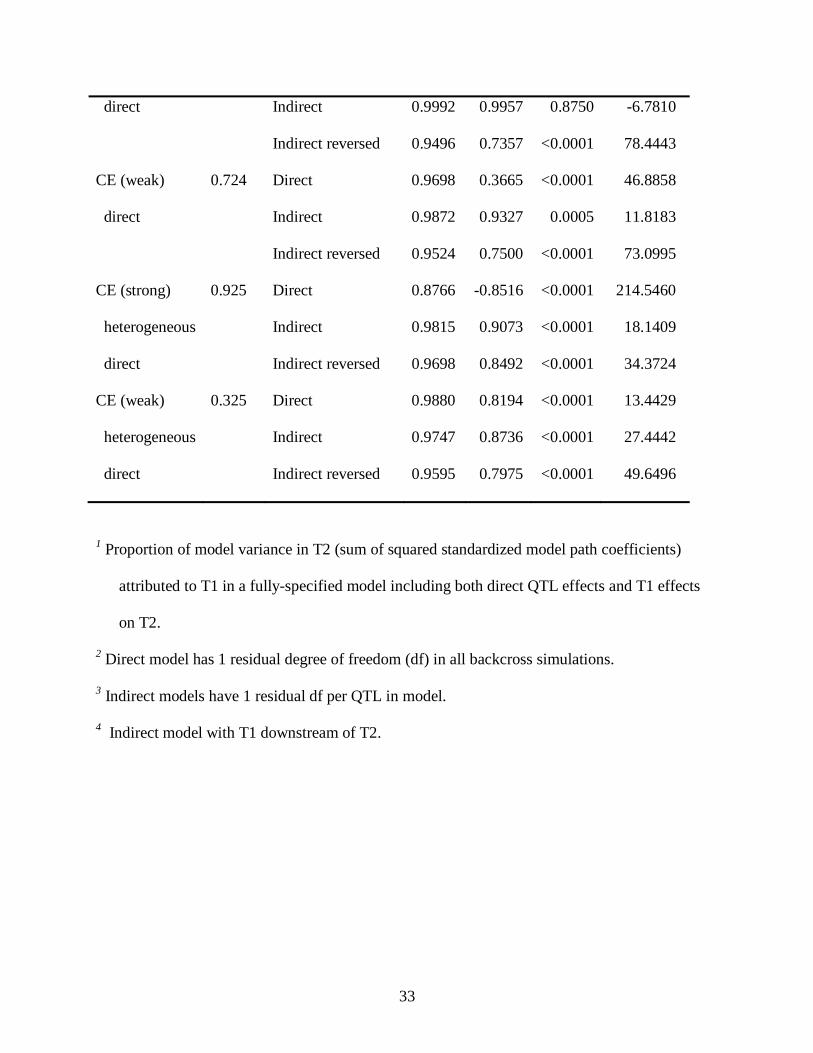
Single QTL in SEM: I also tested the first of the two direct model simulations with three

SEMs that each included only one of the predicted QTLs. Not including all true QTL effects in

the model can be expected to result in residual correlations between the traits, confounding the

“signal” used by SEM to distinguish direct and indirect models. Consistent with this prediction,

the direct model was strongly rejected and the indirect model had higher AIC values in each case

when only one of the three QTLs was included (Table 2). In one case, when only Q3 was

included in the model, the indirect model was found to fit the data adequately (p = 0.1253).

Indirect scenario: When simulations were done under the indirect scenario (Figure 1b),

the indirect model adequately fit the data, with insignificant p-values and negative AIC values,

and correctly performed far better than either the direct model or the indirect model with the trait

effects reversed from the simulated scenario (T2 upstream of T1). In the full model, the

proportion of the effect on T2 inferred to be via the indirect path was greater than 0.98 in both

simulations.

Latent direct scenario: A more complex but potentially realistic scenario was

represented by a pair of simulations in which the QTLs affected an unobserved trait, which in

turn had independent direct effects on T1 and T2 (Figure 1c). The latent direct scenario could

correspond to a situation in which genetic variation in the amount or activity of a transcriptional

regulator affects expression of downstream genes or other observed traits, or any other situation

in which the direct QTL effects are on a trait that is not readily observed. In these simulations,

both the direct and indirect models were rejected, with the direct model showing much poorer fit

18

than the indirect model with T2 downstream but better than the reversed indirect model with T1

downstream. In the full model, proportions of the effects on T2 inferred to come through the

indirect pathway were 0.70 and 0.84 respectively in the two simulations. A SEM corresponding

to the latent direct model is uninformative about the correct scenario due to the model structure,

and thus could not legitimately be tested (see Materials and Methods).

Common-environment direct scenario: The next scenario was one in which T1 and T2

were directly affected by the QTLs as in the direct scenario, but in which common environmental

effects on T1 and T2 were included (CE direct scenario; Figure 1d). This corresponds to a

highly realistic situation in which an environmental variable such as nutrient availability may

jointly affect multiple aspects of growth and development. In the first of these simulations,

common environmental effects were simulated to be strong, explaining 50% of the variance in

T1 and T2. Under this scenario, not only was the indirect model incorrectly favored but it

adequately fit the data, while the direct model and the reversed indirect model were strongly

rejected. In the full model, essentially all of the effect on T2 was inferred to come through the

indirect pathway. In a second simulation, in which the common environmental effect explained

only 15% of the phenotypic variance in both traits, all three of these models were strongly

rejected but the indirect model showed by far the best overall fit. In the full model, the

proportion of the effect on T2 attributed to the indirect path was 0.73.

CE direct scenario with relaxed homogeneity assumptions: There is no particular reason

to expect multiple QTLs to have a homogeneous ratio of effects on multiple traits under a direct-

effects scenario. Thus, I generated additional data sets under the common environmental effects

scenario in which the relative effects of the three QTLs on the two traits were different, to test

whether the direct model would perform better than the indirect model under these relaxed

19

assumptions. Under the CE heterogeneous-direct scenarios, Q1, Q2, and Q3 had larger, equal,

and smaller effects, respectively, on T1 relative to T2, with all three QTLs simulated to have

equal effects on T2. Two data sets were simulated under this scenario, one with strong

correlated environmental effects and the second with weaker correlated effects.

Under both CE heterogeneous-direct scenarios, the fit of the direct model and of both

indirect models were all strongly rejected (Table 1). When the correlated environmental effects

were strong, the indirect model performed best by AIC and adjusted goodness-of-fit criteria,

followed in order by the indirect-reversed and direct models. Under the full model, a proportion

greater than 0.92 of the effects on T2 were attributed to the indirect pathway. When the

correlated environmental effects were weaker, the direct model outperformed the other models

using AIC as the criterion, but the indirect model had the highest adjusted goodness-of-fit.

Under the full model, more than two-thirds of the effect on T2 was attributed to the direct

pathway.

F2 simulations under direct scenario: I also tested SEM performance on F2 progeny

sets simulated under the direct scenario. The additive effects of the three QTLs were simulated

to be the same as those in the backcross simulations. Dominance effects were also simulated,

with d/a ratios differing among QTLs but homogeneous between the two traits. The F2 SEMs

included independent additive and dominance effects for each detected QTL. The SEM results

were similar to those obtained for the direct scenario in the backcross simulations, with the direct

model strongly outperforming the indirect models but still failing as a sufficient explanation of

the data (Table 3). Under the full model, the proportions of the effects on T2 attributed to the

indirect pathway were 0.11 and 0.13, respectively in the two simulations, slightly less than in the

direct-scenario backcross simulations.

20

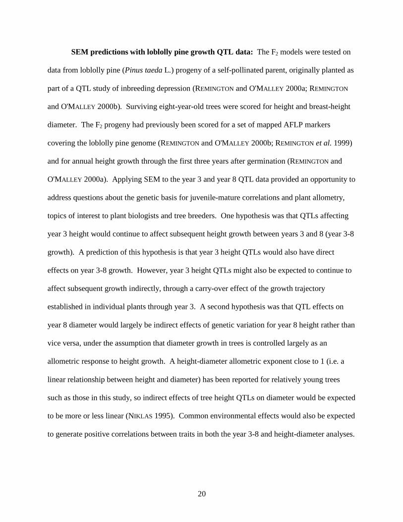
SEM predictions with loblolly pine growth QTL data: The F2 models were tested on

data from loblolly pine (Pinus taeda L.) progeny of a self-pollinated parent, originally planted as

part of a QTL study of inbreeding depression (REMINGTON and O'MALLEY 2000a; REMINGTON

and O'MALLEY 2000b). Surviving eight-year-old trees were scored for height and breast-height

diameter. The F2 progeny had previously been scored for a set of mapped AFLP markers

covering the loblolly pine genome (REMINGTON and O'MALLEY 2000b; REMINGTON et al. 1999)

and for annual height growth through the first three years after germination (REMINGTON and

O'MALLEY 2000a). Applying SEM to the year 3 and year 8 QTL data provided an opportunity to

address questions about the genetic basis for juvenile-mature correlations and plant allometry,

topics of interest to plant biologists and tree breeders. One hypothesis was that QTLs affecting

year 3 height would continue to affect subsequent height growth between years 3 and 8 (year 3-8

growth). A prediction of this hypothesis is that year 3 height QTLs would also have direct

effects on year 3-8 growth. However, year 3 height QTLs might also be expected to continue to

affect subsequent growth indirectly, through a carry-over effect of the growth trajectory

established in individual plants through year 3. A second hypothesis was that QTL effects on

year 8 diameter would largely be indirect effects of genetic variation for year 8 height rather than

vice versa, under the assumption that diameter growth in trees is controlled largely as an

allometric response to height growth. A height-diameter allometric exponent close to 1 (i.e. a

linear relationship between height and diameter) has been reported for relatively young trees

such as those in this study, so indirect effects of tree height QTLs on diameter would be expected

to be more or less linear (NIKLAS 1995). Common environmental effects would also be expected

to generate positive correlations between traits in both the year 3-8 and height-diameter analyses.

21

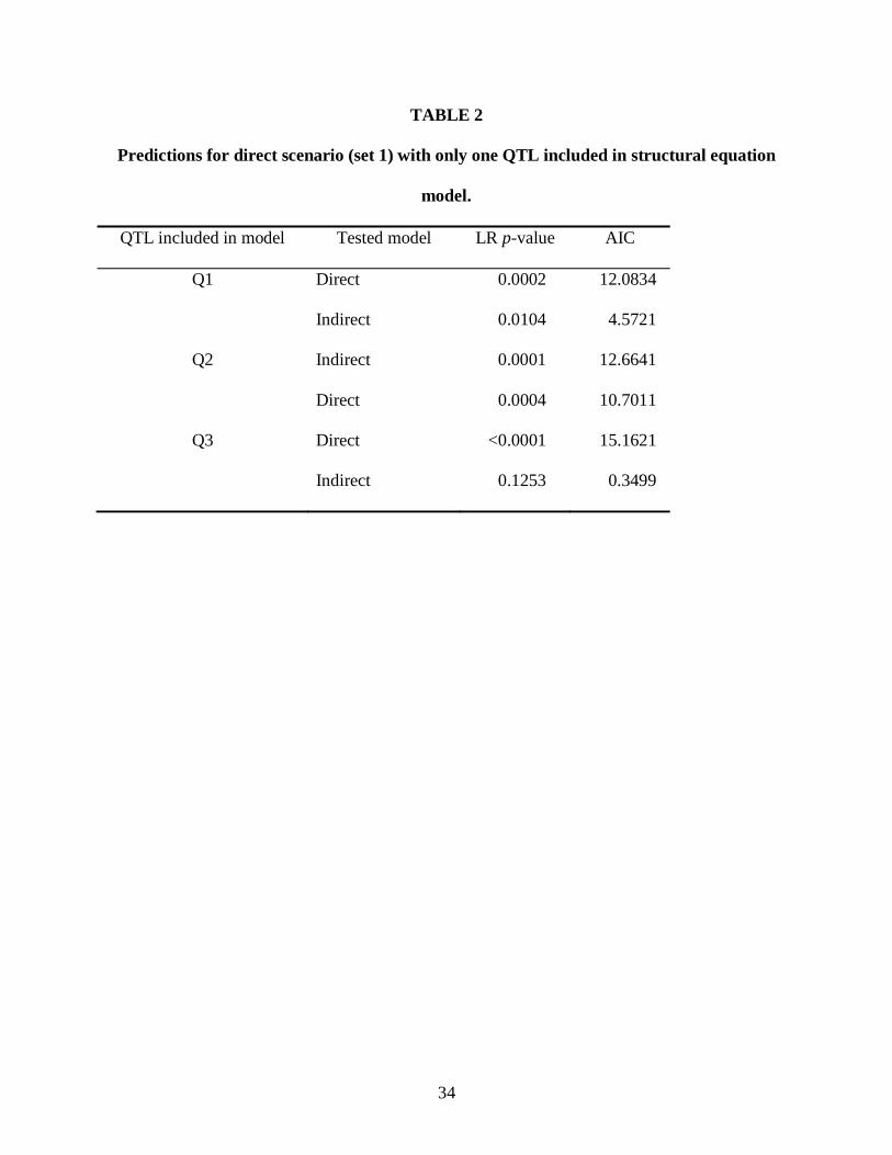
Four QTL regions that exceeded the likelihood ratio test statistic of 16.42 were identified

for eight-year height or diameter. Two QTL regions, LG1-14 and LG8-88, were significant for

both year 8 height and diameter. The LG8-88 region corresponds to the location of the

segregating cad-n1 mutation, which results in production of chemically altered lignin and

reduced wood stiffness, apparently interfering with the trees’ ability to maintain upright form and

sustained height growth (MACKAY et al. 1997; RALPH et al. 1997; REMINGTON and O'MALLEY

2000a). A third QTL region (LG9-08) was significant for year 8 height and strongly suggestive

for diameter (LRT = 16.24). Each of these regions had large additive effects with substantial

overdominance for both traits. A fourth QTL region (LG1-80) was significant for year 8 height,

with large symmetrically overdominant effects, but had no apparent effect on diameter (Table 4).

The height effect associated with LG1-80 may be an artifact of extreme segregation distortion, as

it is flanked by near-lethal recessive alleles linked in repulsion and has substantial deficits of

both homozygous genotypes, but this locus was included in the SEMs anyway to account for all

prospective QTL effects. The LG8-88 and LG1-14 QTL regions had similar effects on height at

earlier ages (REMINGTON and O'MALLEY 2000a). The LG9-08 region was also suggestive of

effects on year 3 growth, with a peak LRT value of 9.18 and additive and dominance effects in

the same direction as in year 8. Two QTL regions on linkage groups 12 (LG12-116) and 3

(LG3-03), which were significant for year 2 and year 3 growth, respectively, had nearly

significant effects on total year 3 height but showed no evidence of effects in year 8. QTL

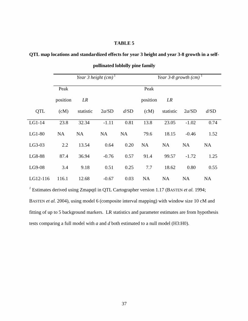
effects for year 3-8 growth were very similar to those for year 8 height (Table 5).

In fitting SEMs for year 3 height and year 3-8 growth, only QTLs with significant or

suggestive effects were included as direct effects; thus, LG12-116 and LG3-03 were only

included in direct effects for year 3 height, and LG1-80 was only included for year 3-8 growth.

22

Similarly, in comparing year 8 height and diameter, LG1-80 was only included in direct effects

for year 8 height. In both cases, QTL regions with direct effects only on the downstream trait

were included in models with indirect effects. The additional degrees of freedom provided by

excluding non-contributing QTLs allowed testing of models that included various combinations

of direct, indirect, and correlated-environment effects on traits.

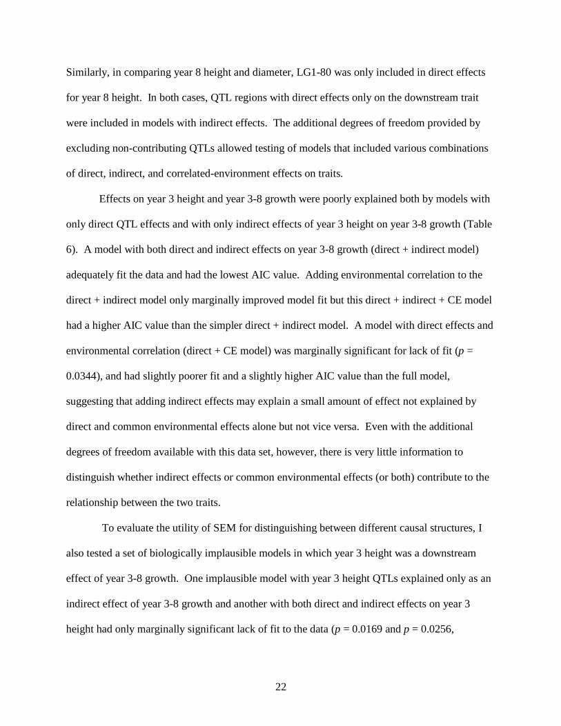
Effects on year 3 height and year 3-8 growth were poorly explained both by models with

only direct QTL effects and with only indirect effects of year 3 height on year 3-8 growth (Table

6). A model with both direct and indirect effects on year 3-8 growth (direct + indirect model)

adequately fit the data and had the lowest AIC value. Adding environmental correlation to the

direct + indirect model only marginally improved model fit but this direct + indirect + CE model

had a higher AIC value than the simpler direct + indirect model. A model with direct effects and

environmental correlation (direct + CE model) was marginally significant for lack of fit (p =

0.0344), and had slightly poorer fit and a slightly higher AIC value than the full model,

suggesting that adding indirect effects may explain a small amount of effect not explained by

direct and common environmental effects alone but not vice versa. Even with the additional

degrees of freedom available with this data set, however, there is very little information to

distinguish whether indirect effects or common environmental effects (or both) contribute to the

relationship between the two traits.

To evaluate the utility of SEM for distinguishing between different causal structures, I

also tested a set of biologically implausible models in which year 3 height was a downstream

effect of year 3-8 growth. One implausible model with year 3 height QTLs explained only as an

indirect effect of year 3-8 growth and another with both direct and indirect effects on year 3

height had only marginally significant lack of fit to the data (p = 0.0169 and p = 0.0256,

23

respectively), and the former had an AIC value within 1.0 of the best-fitting plausible direct +

indirect model.

By contrast, effects on year 8 height and diameter were adequately explained by a model

with only indirect effects of year 8 height on year 8 diameter (Table 7). Models that included

direct QTL effects on both traits in combination with indirect effects on either height or diameter

or correlated environmental effects also adequately fit the data, but had AIC values that were

more than 4.0 larger than the indirect-only model due to the additional degrees of freedom used

in fitting the model. Models with only direct QTL effects on both traits and with height

explained only by diameter failed to fit the data and had much higher AIC values. Thus, the data

are consistent with the prediction that diameter growth is largely an allometric response to height

growth.

DISCUSSION

For this study I used simulations to examine the ability of structural equation models to

distinguish between simple but realistic genetic regulatory scenarios for multiple-trait QTL

mapping data, including those with common environmental effects, incomplete QTL

information, and to examine the sensitivity of SEM to incorrect or incomplete model structures.

The consistent results from the replicate simulations in each case suggest that the patterns they

reveal are valid, and their implications should be taken into account when interpreting the results

of QTL-based causal inference studies.

The correct models were strongly favored using p-value and AIC criteria when data sets

were simulated under direct and indirect scenarios without confounding factors and all QTLs

24

were included in the model. However, the direct model provided only marginal fit to the

simulated data when it was the correct model, which is discussed in more detail below. The

simulated QTL effects were relatively small, with Q2 and Q3 explaining only ~3% of the

phenotypic variance for T2, the trait with smaller QTL effects, in the backcross design. Success

in identifying the correct model in these circumstances is consistent with the results of a larger

set of simulations by Schadt et al. (2005), who found that the power to detect the correct model

under similar circumstances was ~80% when QTLs explained as little as 1-2% of the variation in

the less-affected trait.

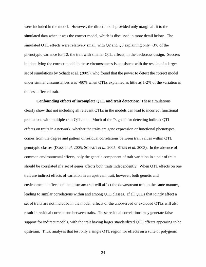
Confounding effects of incomplete QTL and trait detection: These simulations

clearly show that not including all relevant QTLs in the models can lead to incorrect functional

predictions with multiple-trait QTL data. Much of the “signal” for detecting indirect QTL

effects on traits in a network, whether the traits are gene expression or functional phenotypes,

comes from the degree and pattern of residual correlations between trait values within QTL

genotypic classes (DOSS et al. 2005; SCHADT et al. 2005; STEIN et al. 2003). In the absence of

common environmental effects, only the genetic component of trait variation in a pair of traits

should be correlated if a set of genes affects both traits independently. When QTL effects on one

trait are indirect effects of variation in an upstream trait, however, both genetic and

environmental effects on the upstream trait will affect the downstream trait in the same manner,

leading to similar correlations within and among QTL classes. If all QTLs that jointly affect a

set of traits are not included in the model, effects of the unobserved or excluded QTLs will also

result in residual correlations between traits. These residual correlations may generate false

support for indirect models, with the trait having larger standardized QTL effects appearing to be

upstream. Thus, analyses that test only a single QTL region for effects on a suite of polygenic

25

traits are virtually guaranteed to place the traits in a common regulatory pathway, whether such a

pathway exists or not. Even when all experimentally detected QTL regions are included in a

model, some actual QTLs are likely to be missed due to limited experimental power (BEAVIS

1994) and lead to correlated residuals. Testing of direct vs. indirect QTL path models has been

suggested as a test of close linkage vs. pleiotropy with shared QTL regions, since the former are

by definition independently regulated (DOSS et al. 2005; SCHADT et al. 2005). For this test to

identify instances of close linkage effectively, however, these results show that all other QTL

regions that jointly affect the two traits must be included in the model.

Unobserved traits can also affect model predictions if they occur at branching points

leading to observed traits, as in the latent-direct scenario. In the two latent-direct simulations,

neither the direct nor the indirect model was well-supported, providing some indication that the

true model was more complex, but these results are not distinguishable from those expected if

the true scenario were a combination of direct and indirect effects.

Distinguishing indirect vs. common environment effects: These results show that

shared environmental effects on a pair of traits may be difficult to distinguish from indirect

effects. Models combining direct effects with either indirect effects or with common

environmental effects on a pair of traits cannot be distinguished if all QTLs affect both traits;

both will lack residual degrees of freedom and have perfect fit. It should be noted that similar

indistinguishable submodels could potentially be nested within more complex trait networks

even when the overall model has residual degrees of freedom. Even if both model structures can

be tested, however, as with the loblolly pine year 3-8 analyses, there may be little information to

distinguish common environmental effects from indirect effects because both mechanisms will

generate trait correlations within QTL genotype classes. When common environment effects

26

were included in simulations of direct-effects scenarios, indirect models were more strongly

supported in most cases. Genes with smaller standardized genetic effects tended to be placed

downstream of those with larger genetic effects even when their genetic regulation by shared

QTLs was independent.

In biologically realistic situations, shared environmental effects are probably common

because each individual organism in a genetic mapping population is shaped by the unique

environment it has experienced and by the peculiarities of developmental “noise.” These

environmental and developmental effects are likely to have correlated effects on multiple traits

(LYNCH and WALSH 1998). The influence of common environment on residual trait correlations

is well-recognized (DOSS et al. 2005; SCHADT et al. 2005; STEIN et al. 2003) but the question of

whether or not path models can distinguish environmental correlations from causative indirect

effects has received little scrutiny.

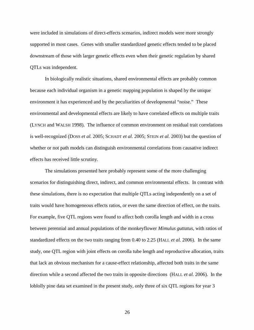
The simulations presented here probably represent some of the more challenging

scenarios for distinguishing direct, indirect, and common environmental effects. In contrast with

these simulations, there is no expectation that multiple QTLs acting independently on a set of

traits would have homogeneous effects ratios, or even the same direction of effect, on the traits.

For example, five QTL regions were found to affect both corolla length and width in a cross

between perennial and annual populations of the monkeyflower Mimulus guttatus, with ratios of

standardized effects on the two traits ranging from 0.40 to 2.25 (HALL et al. 2006). In the same

study, one QTL region with joint effects on corolla tube length and reproductive allocation, traits

that lack an obvious mechanism for a cause-effect relationship, affected both traits in the same

direction while a second affected the two traits in opposite directions (HALL et al. 2006). In the

loblolly pine data set examined in the present study, only three of six QTL regions for year 3

27

height and year 3-8 growth had detectable effects on both traits, and for these three regions the

ratio of standardized homozygous effects on the two traits ranged from 0.44 to 1.09. By contrast,

three QTL regions affecting year 8 height and diameter (ignoring LG1-80, which had negligible

homozygous effects) had standardized effects ratios in a much narrower range of 1.16 to 1.37,

consistent with the SEM inference of indirect effects on diameter. When heterogeneous QTL

effects were simulated, the false support for the indirect model relative to the direct model due to

common environmental effects was weakened or even reversed. Moreover, genetic and

environmental correlations may be in opposite directions in actual trait networks, unlike those in

our simulations. For example, traits involved in life history trade-offs are likely to have negative

genetic correlations, but shared environmental effects (e.g. variation in nutritional status) may

generate positive correlations. In such situations, confounding of common environmental effects

with indirect effects would be unlikely and in some cases SEM results might even be biased

against indirect models.

Sensitivity of the direct models: In contrast with the effects of confounding factors that

favor indirect models, these data show that direct models are highly sensitive to any residual

correlation between trait values. In all four simulations under simple direct-effects scenarios

(two backcross and two F2 simulations), the correct direct model was rejected as an adequate

explanation of the data (LR p-values < 0.05) even though it outperformed the indirect model.

Concomitantly, the full models that included both direct and indirect effects estimated as much

as 20% of the effect on T2 to occur via the indirect pathway under the direct-effects scenarios,

even though none of the actual effect was indirect. The basis for this bias toward indirect effects

is uncertain. Imprecise estimates of the true QTL locations is one possibility, although replacing

the estimated QTL locations with the actual simulated locations in one of the simulations did not

28

improve the fit (data not shown). Imprecise estimates of the true QTL effects will result in

under- or over-fitting of the model to the true sources of effects, and could also result in residual

correlations. It is also possible that the residual values generated in the QTL Cartographer

simulations were not entirely random.

Regardless of the explanation for the lack of complete model fit in the simulated data,

actual data from directly-regulated trait sets can generally be expected to show even less

independence of residuals due to the pervasiveness of common environmental effects and

undetected QTLs discussed above. Given these realities, standard tests of model fit are

inappropriate for evaluating the sufficiency of direct-effects models. Empirical tests will be

necessary but not easy to implement, as permutation tests would have to randomize trait values

within QTL classes and handling recombinants will present special problems. Parametric

bootstrap simulations may be a better option, but the algorithms required to generate hundreds of

simulated datasets, estimate QTL locations and virtual marker scores, and run multiple SEMs on

each simulation will be complex. Effects of unobserved QTLs could be incorporated as

polygenic effects in a parametric bootstrap. Crude but potentially useful estimates of polygenic

variance could be obtained from the percentage of differences between parental lines not

explained by the identified QTLs, especially if the mapping population were derived from

divergent parental lines.

In spite of the factors causing bias against the direct model, direct effects were identified

as the largest contributor to QTL effects in the experimental data on loblolly pine year 3-8

growth. These results were consistent with a priori predictions of carryover effects of earlier

QTL action and possibly common environment effect as additional contributors to year 3-8

29

growth. In contrast, QTL effects on year 8 diameter were fully explained as an indirect effect of

year 8 height, also consistent with a priori predictions based on allometry theory.

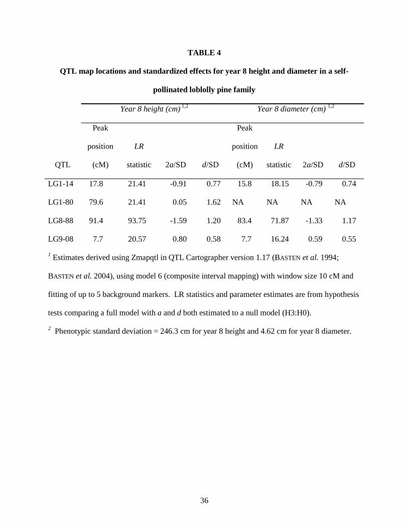
Limitations of SEM for exploratory analysis: Results of this study underscore the

need for caution in using SEM in a purely exploratory mode in the absence of functional

hypotheses to guide the choice of model structure. While SEM analyzes causal models of the

covariance structure between traits, the adequate fit of a model does not by itself imply causation

(GRACE and PUGESEK 1998; MITCHELL 1992). In data sets simulated under an indirect scenario,

reversing the cause-effect relationship between the two traits resulted in substantially poorer

model fit, as expected. With the loblolly pine year 3 – year 8 height data, however, a

biologically implausible but simple model in which year 3-8 growth alone explained year 3

height QTLs fit nearly as well as the best-fitting plausible model, which required both direct and

indirect QTL effects to explain year 3-8 growth, and fit better than any of the other plausible

models tested. The most likely explanation is that the standardized effect of QTLs on year 3-8

growth is much larger than on year 3 height due to the very large effect of the LG8-88 QTL on

year 3-8 growth. In this example, the temporal relationship between the traits made the

distinction between plausible vs. implausible model structures obvious, but this will not be the

case in other situations. For example, in explaining genetic correlations between morphological

and physiological traits, reasonable biological models might involve direct or indirect genetic

effects on either set of traits. It is therefore important to include as much prior biological

information as possible to identify plausible networks, such as prior information on co-regulated

sets of genes or structure of known regulatory pathways in eQTL analyses (KEURENTJES et al.

2007; KLIEBENSTEIN et al. 2006; ZHU et al. 2008), developmental models describing temporal

and functional relationships among morphological and physiological traits (MÜNDERMANN et al.

30

2005), and the expected direction of correlations of common environmental effects. In this

context, SEM provides a powerful tool for testing the adequacy of causal hypotheses (MITCHELL

1992). Purely exploratory analyses may be useful in systems-biology applications for reducing

the set of model structures for further experimentation (or "sparsification", per LIU et al. 2008),

but the results of such analyses should not be interpreted as support for particular causal

structures.

Summary: Results of this study confirm that the residual correlation structure in

multiple-trait QTL data, which is typically unused in QTL analyses, provides a powerful but

limited source of information on the functional basis of trait variation. Factors likely to be

pervasive in real biological data, including common environmental effects and incomplete

identification of QTLs, can masquerade as indirect causal effects and lead to incorrect

conclusions if not carefully considered. Applications of SEM or other approaches to path

analysis for functional predictions from QTL data need to incorporate as much a priori

information as possible on the traits being studied, including the expected patterns of common

environmental effects on traits, if the predictions are to be biologically useful.

Further studies should be conducted to test the predictive power of SEM under scenarios

such as the ones used here. Other studies have used large numbers of simulations to examine the

power of network modeling approaches (LIU et al. 2008; NETO et al. 2008; SCHADT et al. 2005),

but have not explored the questions addressed in the present study. Issues with statistically

indistinguishable models incorporating common environment vs. indirect effects need to be

examined in more complex trait networks, where untestable fully-specified modules may be

nested within larger models. Future research needs also include evaluating different patterns of

31

direct genetic and common environmental effects, developing methods for empirical statistical

tests, and incorporating epistatic QTL effects.

I thank Ross Whetten and Elizabeth Lacey for assistance with year 8 data collection from the

Tillman, SC loblolly pine genetic mapping population; Rongling Wu for first suggesting to me

the use of path analysis approaches for functional prediction from QTL data; Elizabeth Lacey,

Sergey Nuzhdin, and David Aylor for valuable discussions; and Malcolm Schug, Rebecca

Doerge, and two anonymous reviewers for helpful comments to improve the manuscript.

32

TABLE 1

Summary of structural equation model analyses for backcross simulations

Simulated

scenario

T2

VI /VQ 1

Tested model GFI AGFI LR p-

value

AIC

Direct (set 1) 0.165 Direct 2 0.9962 0.9432 0.0291 2.7627

Indirect 3 0.9810 0.9052 <0.0001 18.6995

Indirect reversed 4 0.9332 0.6660 <0.0001 92.3938

Direct (set 2) 0.196 Direct 0.9955 0.9332 0.0178 3.6130

Indirect 0.9825 0.9125 <0.0001 16.7255

Indirect reversed 0.9408 0.7042 <0.0001 79.3354

Indirect (set 1) 0.989 Direct 0.8440 -1.3404 <0.0001 307.5001

Indirect 0.9955 0.9776 0.1297 -0.3460

Indirect reversed 0.9553 0.7767 <0.0001 56.0307

Indirect (set 2) 0.985 Direct 0.8880 -2.1365 <0.0001 288.6861

Indirect 0.9964 0.9800 0.2796 -3.7162

Indirect reversed 0.9804 0.8904 <0.0001 26.1377

Latent direct 0.844 Direct 0.9591 0.3861 <0.0001 54.2958

(set 1) Indirect 0.9907 0.9537 0.0081 5.7892

Indirect reversed 0.9381 0.6904 <0.0001 83.9911

Latent direct 0.696 Direct 0.9594 0.3903 <0.0001 53.8670

(set 2) Indirect 0.9810 0.9048 <0.0001 18.8166

Indirect reversed 0.9477 0.7387 <0.0001 68.0184

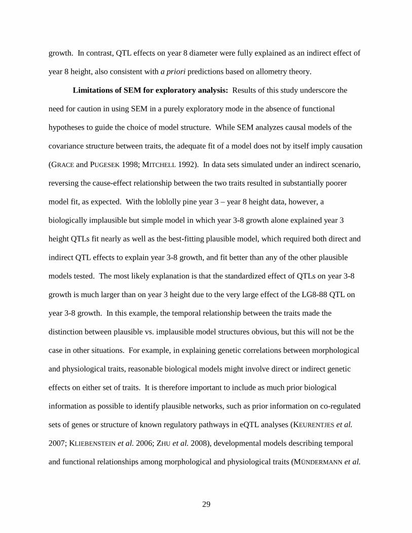
CE (strong) 0.999 Direct 0.8987 -1.1270 <0.0001 203.9092

33

direct Indirect 0.9992 0.9957 0.8750 -6.7810

Indirect reversed 0.9496 0.7357 <0.0001 78.4443

CE (weak) 0.724 Direct 0.9698 0.3665 <0.0001 46.8858

direct Indirect 0.9872 0.9327 0.0005 11.8183

Indirect reversed 0.9524 0.7500 <0.0001 73.0995

CE (strong) 0.925 Direct 0.8766 -0.8516 <0.0001 214.5460

heterogeneous Indirect 0.9815 0.9073 <0.0001 18.1409

direct Indirect reversed 0.9698 0.8492 <0.0001 34.3724

CE (weak) 0.325 Direct 0.9880 0.8194 <0.0001 13.4429

heterogeneous Indirect 0.9747 0.8736 <0.0001 27.4442

direct Indirect reversed 0.9595 0.7975 <0.0001 49.6496

1 Proportion of model variance in T2 (sum of squared standardized model path coefficients)

attributed to T1 in a fully-specified model including both direct QTL effects and T1 effects

on T2.

2 Direct model has 1 residual degree of freedom (df) in all backcross simulations.

3 Indirect models have 1 residual df per QTL in model.

4 Indirect model with T1 downstream of T2.

34

TABLE 2

Predictions for direct scenario (set 1) with only one QTL included in structural equation

model.

QTL included in model Tested model LR p-value AIC

Q1 Direct 0.0002 12.0834

Indirect 0.0104 4.5721

Q2 Indirect 0.0001 12.6641

Direct 0.0004 10.7011

Q3 Direct <0.0001 15.1621

Indirect 0.1253 0.3499

35

TABLE 3

Summary of structural equation model analyses for F2 simulations

Simulated

scenario

T2

VI /VQ 1

Tested model GFI AGFI LR p-

value

AIC

Direct (set 1) 0.105 Direct 0.9963 0.7948 0.0021 7.4309

Indirect 0.9721 0.8082 <0.0001 61.2901

Indirect reversed 0.9306 0.5229 <0.0001 216.8199

Direct (set 2) 0.134 Direct 0.9957 0.7624 0.0009 8.9432

Indirect 0.9760 0.8351 <0.0001 49.4271

Indirect reversed 0.9398 0.5863 <0.0001 176.5202

1 Proportion of model variance in T2 (sum of squared standardized model path coefficients)

attributed to T1 in a fully-specified model including both direct QTL effects and T1 effects

on T2.

2 Direct model has 1 residual df.

3 Indirect models have 2 residual df per QTL in model.

36

TABLE 4

QTL map locations and standardized effects for year 8 height and diameter in a self-

pollinated loblolly pine family

Year 8 height (cm) 1,2 Year 8 diameter (cm) 1,2

QTL

Peak

position

(cM)

LR

statistic 2a/SD d/SD

Peak

position

(cM)

LR

statistic 2a/SD d/SD

LG1-14 17.8 21.41 -0.91 0.77 15.8 18.15 -0.79 0.74

LG1-80 79.6 21.41 0.05 1.62 NA NA NA NA

LG8-88 91.4 93.75 -1.59 1.20 83.4 71.87 -1.33 1.17

LG9-08 7.7 20.57 0.80 0.58 7.7 16.24 0.59 0.55

1 Estimates derived using Zmapqtl in QTL Cartographer version 1.17 (BASTEN et al. 1994;

BASTEN et al. 2004), using model 6 (composite interval mapping) with window size 10 cM and

fitting of up to 5 background markers. LR statistics and parameter estimates are from hypothesis

tests comparing a full model with a and d both estimated to a null model (H3:H0).

2 Phenotypic standard deviation = 246.3 cm for year 8 height and 4.62 cm for year 8 diameter.

37

TABLE 5

QTL map locations and standardized effects for year 3 height and year 3-8 growth in a self-

pollinated loblolly pine family

Year 3 height (cm) 1 Year 3-8 growth (cm) 1

QTL

Peak

position

(cM)

LR

statistic 2a/SD d/SD

Peak

position

(cM)

LR

statistic 2a/SD d/SD

LG1-14 23.8 32.34 -1.11 0.81 13.8 23.05 -1.02 0.74

LG1-80 NA NA NA NA 79.6 18.15 -0.46 1.52

LG3-03 2.2 13.54 0.64 0.20 NA NA NA NA

LG8-88 87.4 36.94 -0.76 0.57 91.4 99.57 -1.72 1.25

LG9-08 3.4 9.18 0.51 0.25 7.7 18.62 0.80 0.55

LG12-116 116.1 12.68 -0.67 0.03 NA NA NA NA

1 Estimates derived using Zmapqtl in QTL Cartographer version 1.17 (BASTEN et al. 1994;

BASTEN et al. 2004), using model 6 (composite interval mapping) with window size 10 cM and

fitting of up to 5 background markers. LR statistics and parameter estimates are from hypothesis

tests comparing a full model with a and d both estimated to a null model (H3:H0).

38

TABLE 6

Summary of structural equation model analyses on loblolly pine year 3 height and year 3-8

height growth QTL data

Tested model Year 3-8

VI /VQ 1

df

GFI AGFI LR

p-value

AIC

Direct + indirect 0.453 6 0.9886 0.8006 0.0689 -0.2958

Direct + reversed indirect 2 6 0.9861 0.7566 0.0256 2.3834

Direct 7 0.9486 0.2286 <0.0001 53.6942

Direct + CE 6 0.9867 0.7671 0.0344 1.5998

Indirect 12 0.9346 0.4276 <0.0001 65.2851

Reversed indirect 12 0.9771 0.7995 0.0169 0.5877

Direct + indirect + CE 5 0.9895 0.7792 0.0558 0.7843

1 Proportion of model variance in year 3-8 growth (sum of squared standardized model path

coefficients) attributed to year 3 height in a fully-specified model including both direct QTL

effects and year 3 height effects on year 3-8 growth.

2 Indirect model with year 3 height downstream of year 3-8 growth.

39

TABLE 7

Summary of structural equation model analyses on loblolly year 8 height and diameter

QTL data

Tested model Diam

VI /VQ 1

df

GFI AGFI LR

p-value

AIC

Direct + indirect 0.981 2 0.9993 0.9802 0.7730 -3.4851

Direct + reversed indirect 2 2 0.9951 0.8643 0.1660 -0.4087

Direct 3 0.8978 -0.8739 <0.0001 114.4400

Direct + CE 2 0.9951 0.8642 0.1658 -0.4059

Indirect 8 0.9890 0.9245 0.4171 -7.8308

Reversed indirect 8 0.9513 0.6651 <0.0001 25.0491

1 Proportion of model variance in year 8 diameter (sum of squared standardized model path

coefficients) attributed to year 8 height in a fully-specified model including both direct QTL

effects and year 8 height effects on year 8 diameter.

2 Indirect model with year 8 height downstream of year 8 diameter.

40

Figure caption:

FIGURE 1.– Path models for scenarios simulated or modeled in this study: a. direct-effects

scenario; b. indirect scenario; c. latent direct scenario; d. direct-effects scenario with common

environment effects (direct CE scenario); e. direct CE scenario with heterogeneous QTL effect

ratios; f. full model including both direct effects and indirect effects on T2. In these diagrams,

Q1, Q2, and Q3 represent simulated QTLs, T1 and T2 represent observed traits, T0 represents an

unobserved (latent) trait, and EC represents common environmental effects.

41

a.

b.

c.

d.

e.

f.

Q1Q2Q3

T1

T2 EC

Q1Q2Q3

T1

T2

T0 Q1Q2Q3

T1

T2

T1

T2 EC

Q1

Q2

Q3

Q1Q2Q3

T2 T1

Q1Q2Q3

T1

T2

42

LITERATURE CITED

AKAIKE, H., 1974 A new look at the statistical identification model. IEEE T. Automat. Contr. 19:

716-723.

AKAIKE, H., 1987 Factor analysis and AIC. Psychometrika 52: 317-332.

AMOS DEVELOPMENT CORPORATION, 2006 Amos 7.0.0, pp. Amos Development Corporation,

Spring House, PA.

BASTEN, C. J., B. S. WEIR and Z.-B. ZENG, 1994 Zmap-a QTL cartographer., pp. 65-66 in 5th

World Congress on Genetics Applied to Livestock Production: Computing Strategies and

Software., edited by C. SMITH, J. S. GAVORA, B. BENKEL, J. CHESNAIS, W. FAIRFULL et

al. Organizing Committee, 5th World Congress on Genetics Applied to Livestock

Production., Guelph, Ontario, Canada.

BASTEN, C. J., B. S. WEIR and Z.-B. ZENG, 2004 QTL Cartographer, Version 1.17, pp.

Department of Statistics, North Carolina State University, Raleigh, NC.

BEAVIS, W. D., 1994 The power and deceit of QTL experiments: lessons from comparative QTL

studies. Proceedings of the 49th Annual Corn and Sorghum Industry Research

Conference, Chicago 49: 250-266.

BENFEY, P. N., and T. MITCHELL-OLDS, 2008 From genotype to phenotype: systems biology

meets natural variation. Science 320: 495-497.

BREM, R. B., G. YVERT, R. CLINTON and L. KRUGLYAK, 2002 Genetic dissection of

transcriptional regulation in budding yeast. Science 296: 752-755.

43

BREWER, M. T., J. B. MOYSEENKO, A. J. MONFORTE and E. VAN DER KNAAP, 2007

Morphological variation in tomato: a comprehensive study of quantitative trait loci

controlling fruit shape and development. J. Exp. Bot. 58: 1339-1349.

DOSS, S., E. E. SCHADT, T. A. DRAKE and A. J. LUSIS, 2005 Cis-acting expression quantitative

trait loci in mice. Genome Res. 15: 681-691.

FEDER, M. E., and T. MITCHELL-OLDS, 2003 Evolutionary and ecological functional genomics.

Nat. Rev. Genet. 4: 651-657.

GRACE, J. B., and B. H. PUGESEK, 1998 On the use of path analysis and related procedures for the

investigation of ecological problems. Am. Nat. 152: 151-159.

HALL, M. C., C. J. BASTEN and J. H. WILLIS, 2006 Pleiotropic quantitative trait loci contribute to

population divergence in traits associated with life-history variation in Mimulus guttatus.

Genetics 172: 1829-1844.

JIANG, C.-J., and Z. B. ZENG, 1995 Multiple trait analysis of genetic mapping for quantitative

trait loci. Genetics 140: 1111-1127.

KEURENTJES, J. J. B., J. FU, C. H. RIC DE VOS, A. LOMMEN, R. D. HALL et al., 2006 The genetics

of plant metabolism. Nature Genet. 38: 842-849.

KEURENTJES, J. J. B., J. FU, I. R. TERPSTRA, J. M. GARCIA, G. VAN DEN ACKEVEKEN et al., 2007

Regulatory network construction in Arabidopsis by using genome-wide gene expression

quantitative trait loci. Proc. Natl. Acad. Sci. USA 104: 1708-1713.

KEURENTJES, J. J. B., M. KOORNNEEF and D. VREUGDENHIL, 2008 Quantitative genetics in the

age of omics. Curr. Opin. Plant Biol. 11: 123-128.

44

KLIEBENSTEIN, D. J., M. A. L. WEST, H. VAN LEEUWEN, O. LOUDET, R. W. DOERGE et al., 2006

Identification of QTLs controlling gene expression networks defined a priori. BMC

Bioinformatics 7: 308.

KOONIN, E. V., and Y. I. WOLF, 2008 Evolutionary systems biology, pp. 11-25 in Evolutionary

Genomics and Proteomics, edited by M. PAGEL and A. POMIANKOWSKI. Sinauer,

Sunderland, MA.

LANGLADE, N. B., X. FENG, T. DRANSFIELD, L. COPSEY, A. I. HANNA et al., 2005 Evolution

through genetically controlled allometry space. Proc. Natl. Acad. Sci. USA 102: 10221-

10226.

LI, R., S.-W. TSAIH, K. SHOCKLEY, I. M. STYLIANOU, J. WERGEDAL et al., 2006 Structural model

analysis of multiple quantitative traits. PLoS Genetics 2: e114.

LISEC, J., R. C. MEYER, M. STEINFATH, H. REDESTIG, M. BECHER et al., 2008 Identification of

metabolic and biomass QTL in Arabidopsis thaliana in a parallel analysis of RIL and IL

populations. Plant J. 53: 960-972.

LIU, B., A. DE LA FUENTE and I. HOESCHELE, 2008 Gene network inference via structural

equation modeling in genetical genomics experiments. Genetics 178: 1763-1776.

LYNCH, M., and B. WALSH, 1998 Genetics and Analysis of Quantitative Traits. Sinauer,

Sunderland, MA.

MACKAY, J. J., D. M. O'MALLEY, T. PRESNELL, F. L. BOOKER, M. M. CAMPBELL et al., 1997

Inheritance, gene expression, and lignin characterization in a mutant pine deficient in

cinnamyl alcohol dehydrogenase. Proc. Natl. Acad. Sci. USA 94: 8255-8260.

MACKAY, T. F. C., 2001 The genetic architecture of quantitative traits. Ann. Rev. Genet. 35: 303-

339.

45

MACKAY, T. F. C., 2004 Genetic dissection of quantitative traits., pp. 51-73 in The Evolution of

Population Biology, edited by R. S. SINGH and M. Y. UYENOYAMA. Cambridge

University Press, Cambridge, UK.

MITCHELL, R. J., 1992 Testing evolutionary and ecological hypotheses using path analysis and

structural equation modeling. Funct. Ecol. 6: 123-129.

MÜNDERMANN, L., Y. ERASMUS, B. LANE, E. COEN and P. PRUSINKIEWICZ, 2005 Quantitative

modeling of Arabidopsis development. Plant Physiol. 139: 960-968.

NETO, E. C., C. T. FERRARA, A. D. ATTIE and B. S. YANDELL, 2008 Inferring causal phenotype

networks from segregating populations. Genetics 179: 1089-1100.

NIKLAS, K. J., 1995 Size-dependent allometry of tree height, diameter and trunk-taper. Ann. Bot.

75: 217-227.

RALPH, J., J. J. MACKAY, R. D. HATFIELD, D. M. O'MALLEY, R. W. WHETTEN et al., 1997

Abnormal lignin in a loblolly pine mutant. Science 277: 235-239.

RAUH, B. L., C. BASTEN and E. S. BUCKLER, 2002 Quantitative trait loci analysis of growth

response to varying nitrogen sources in Arabiodpsis thaliana. Theor. Appl. Genet. 104:

743-750.

REMINGTON, D. L., and D. M. O'MALLEY, 2000a Evaluation of major genetic loci contributing to

inbreeding depression for survival and early growth in a selfed family of Pinus taeda.

Evolution 54: 1580-1589.

REMINGTON, D. L., and D. M. O'MALLEY, 2000b Whole-genome characterization of embryonic

stage inbreeding depression in a selfed loblolly pine family. Genetics 155: 337-348.

46

REMINGTON, D. L., R. W. WHETTEN, B.-H. LIU and D. M. O'MALLEY, 1999 Construction of an

AFLP genetic map with nearly complete genome coverage in Pinus taeda. Theor. Appl.

Genet. 98: 1279-1292.

SAS INSTITUTE INC., 2002 The SAS System for Windows, version 9.1, pp., Cary, NC.

SCHADT, E. E., J. LAMB, X. YANG, J. ZHU, S. EDWARDS et al., 2005 An integrative genomics

approach to infer causal associations between gene expression and disease. Nature Genet.

37: 710-717.

STEIN, C. M., Y. SONG, R. C. ELSTON, G. JUN, H. K. TIWARI et al., 2003 Structural equation

model-based genome scan for the metabolic syndrome. BMC Genetics 4(Suppl 1): S99.

TONSOR, S. J., and S. M. SCHEINER, 2007 Plastic trait integration across a CO2 gradient in

Arabidopsis thaliana. Am. Nat. 169: E119-E140.

WRIGHT, S., 1921 Correlation and causation. Journal of Agricultural Research 20: 557-585.

ZHU, J., P. Y. LUM, J. LAMB, D. GUHATHAKTURA, S. W. EDWARDS et al., 2004 An integrative

genomics approach to the reconstruction of gene networks in segregating populations.

Cytogenet. Genome Res. 105: 363-374.

ZHU, J., B. ZHANG, E. N. SMITH, B. DREES, R. B. BREM et al., 2008 Integrating large-scale

functional genomic data to dissect the complexity of yeast regulatory networks. Nature

Genet. 40: 854-861.