University of Central Florida University of Central Florida

STARS STARS

Retrospective Theses and Dissertations

1984

Effects of Finite Length Registers on a Modified Directform Effects of Finite Length Registers on a Modified Directform

Realization of a High Order H(z) Transfer Function Realization of a High Order H(z) Transfer Function

Angel Vanrell University of Central Florida

Part of the Engineering Commons

Find similar works at: https://stars.library.ucf.edu/rtd

University of Central Florida Libraries http://library.ucf.edu

This Masters Thesis (Open Access) is brought to you for free and open access by STARS. It has been accepted for

inclusion in Retrospective Theses and Dissertations by an authorized administrator of STARS. For more information,

please contact STARS@ucf.edu.

STARS Citation STARS Citation Vanrell, Angel, "Effects of Finite Length Registers on a Modified Directform Realization of a High Order H(z) Transfer Function" (1984). Retrospective Theses and Dissertations. 4707. https://stars.library.ucf.edu/rtd/4707

EFFECTS OF FINITE LENGTH REGISTERS ON A MODIFIED DIRECT-FORM REALIZATION OF A HIGH ORDER H(z) TRANSFER FUNCTION

BY

ANGEL VANRELL, III B.S .E.E., University of Florida, 1981

RESEARCH REPORT

Submitted in partial fulfillment of requirements for the degree of Master of Science in Engineering

in the Graduate Studies Program of the College of Engineering

University of Central Florida Orlando, Florida

Summer Term 1984

ACKNOWLEDGEMENTS

I wish to thank the management of Martin Marietta's Engineering

Computing Center for supporting this work and Dr. Fred 0. Simons for his

advice during my graduate program.

i i i

TABLE OF CON TENTS

LI ST OF FIGURES v

LIST OF TABLES . . . . . . . . . . . . . . . . . . . . . . . . . . . . . . . . . . . . . . . . . . . . . . . . . . . . . vi

CHAPTER

I. INTRODUCTION 1

II. EFFECTS OF FINITE WORD LENGTH . . . . . . . . . . . . ..... ... . ........ .. 3

III. DEVELOPMENT OF REALIZATON SCHEMES ........................... 16

IV. EMULATION OF DIGITAL PROCESSES . . . . . . . . . . . . . . . . . . . . . . . . . . . . . . 23

V. TEST CASE: A FOURTH-ORDER LOW-PASS BUTTERWORTH FILTER . . . . . . . . . . . . . . . . . . . . . . . . . . . . . . . . . . . . . . . . . . 30

VI. CONCLUSION . . . . . . . . . . . . . . . . . . . . . . . . . . . . . . . . . . . . . . . . . . . . . . . . . . 40

APPENDIX . . . . . . . . . . . . . . . . . . . . . . . . . . . . . . . . . . . . . . . . . . . . . . . . . . . . . . . . . . . 42

LI ST OF REFERENCES . . . . . . . . . . . . . . . . . . . . . . . . . . . . . . . . . . . . . . . . . . . . . . . . . 48

iv

1.

2.

3.

4.

5.

6.

LIST OF FIGURES

Statistical Model of a Digital Multiplier

Direct, Cascade, and Parallel Realizations

Modified Direct-Form Achitecture

Canonic Direct-Form Architecture

Roundoff Error Algorithm

Single- and Mixed-Precision Arithmetic

7. Frequency Response to the Fourth -Order

10

13

14

15

26

38

Low-Pass Butterworth Digital Filter .......................... 31

8. Mechanization of the Modified Direct-Form 34

9. Mechanization of the Canonic Direct-Form 35

10. Block Diagram of a MAC Device 43

v

1.

2.

3 .

4.

5.

6.

LIST OF TABLES

Feedforward Coefficients

Feedback Coefficients of Canoni c Di rect-Form . . ............... .

Feedback Coefficients of th e Mod i fie d Direct-Form ............ .

Scaling Parameters

Statistics on Noise Sources

Statistics on etot Versus Word Length .. . . . .. ................. .

vi

32

32

32

32

37

37

ABSTRACT

When a digital process is realized on a general-purpose computer

or a special-purpose hardware, errors due to finite register length are

introduced. These errors are due primarily to arithmetic roundoff,

coefficient quantization, and scaling rules. This paper addresses the

effects of finite word length on a direct-form implementation of a high

order H(z) transfer function.

The development and analysis of a modified direct-form realization

suggested by Dr. Fred 0. Simons, are carried out via FORTRAN emulation

of a fourth-order low-pass Butterworth filter. The results are

presented as a parametric tradeoff of signal-to-noise ratio at the

filter output versus word length. Conclusions are drawn by comparing the

modified direct-form with the canonic direct-form. The analysi s

presented here is intended to illustrate how a high order transfer

function can be realized directly without decomposing into a group of

low-order subfilters.

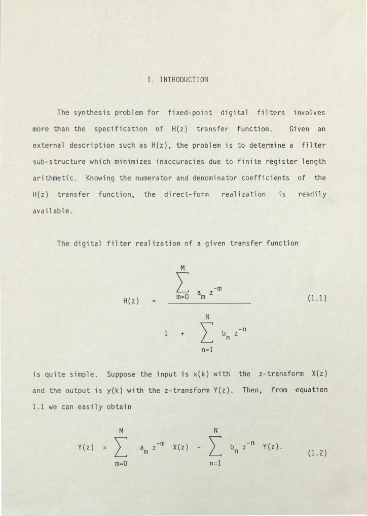
I. I NTROOUCT ION

The synthesis problem for fixed - point dig ital filters involves

more than the specification of H( z ) t ra nsfer function. Given an

external description such as H(z), the probl em is to determine a filter

sub-structure which minimizes inaccuracies due to fin ite register length

arithmetic. Knowing the numerator and denominator coeff icients of the

H(z) transfer function, the direct- form reali zat i on is readily

available.

The digital filter realization of a given transf er fu nction

M

L -m a z H(z) m=O m

= ( 1.1)

N

1 L b - n

+ z n

n=l

is quite simple. Suppose the input is x(k) wi t h the z-transform X(z)

and the output is y(k) with the z-t r an sf orm Y(z ) . Then, from equation

1.1 we can easily obtain

M

Y(z) =L X(z)

m=O

N

L n=l

b n

-n z y ( z). ( 1. 2)

2

From equation 1.2 and applying the inverse z-transform, we obtain

the discrete time domain equation

y(k)

M

L am x(k-m)

m=O

N

L n=l

b y(k-n) n

( 1. 3)

which is the difference (or delay) equation that realizes H(z) directly,

and which also represents a computational algorithm.

In the absence of a finite word length effects, synthesis of

equation 1.1 is trivial. However, such a realization can produce

inaccuracy which is orders of magnitude greater than other realizations.

Therefore the cardinal rule, described by Kaiser [l], is to use a

design method that permits decomposition of the higher order filter into

a group of low-order (first- or second-order) subfilters. This is a

well documented fact. However, we intend to introduce a architecture

with its corresponding algorithm which can match the performance of the

decomposed architectures.

II. EFFECTS OF FINITE WORD LENGTH

A digital filter is represented by a linear shift-invariant

discrete transfer function of the form

M

H(z)

L m=O ( 2. 1)

1

n=l

realized with finite accuracy in the representation of all data and

parameter values. A di g i ta l f i l te r can be simulated on a

general-purpose computer or can be constructed with special-purpose

hardware. Despite the many advantages provided by a digital filter,

there is an inherent limitation on the accuracy of these filters, due to

t he fact that all digital architectures operate with a finite word

length. Any digital transfer function can be implemented in a multitude

of configurations. In a given digital filter architecture, the effect of

finite word length results in three primary sources of error:

1. Input-quantization errors due to the analog-to-digital

conversion of an analog signal,

2. coefficient-quantization due to the representation of the

filter coefficients a and b by a finite number of m n

bits, and

3

4

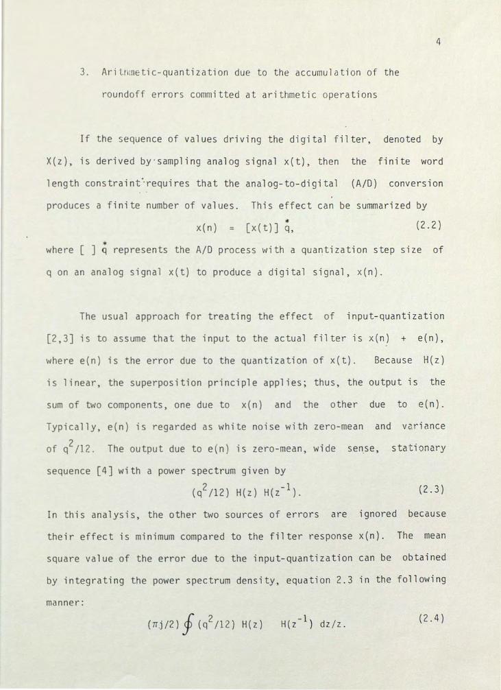
3. Arittmetic-quantization due to the accumulation of the

roundoff errors committed at arithmetic operatio ns

If the sequence of values driving the digital filter, denoted by

X(z), is derived by·sampling analog signal x(t), then the finite word

length constraint~requires that the analog-to-digital (A/D) conversion

produces a finite number of values. This effect can be summarized by

x(n) * [x(t)] q, (2.2)

* where [ ] q represents the A/D process with a quantization step size of

q on an analog signal x(t) to produce a digital signal, x( n).

The usual approach for treating the effect of input-quantization

[2,3] is to assume that the input to the actual filter is x(n) + e(n),

vhere e(n) is the error due to the quantization of x(t). Because H(z)

is linear the superposition principle applies; thus, the output is the

sum of two components, one due to x(n) and the other due to e(n).

Typically e(n) is regarded as white noise with zero-mean and variance

2 of q /12. The output due to e(n) is zero-mean wide se~se, stationary

sequence [4] with a power spectrum given by

(q2/12) H(z) H(z- 1). (2.3)

In this analysis, the other two sources of errors are ignored because

their effect is minimum compared to the filter response x(n). The mean

square value of the error due to the input-quantization can be obtained

by integrating the power spectrum density, equation 2.3 in the following

manner:

(11j/2) § (q2!12) H(z)

-1 H(z ) dz / z.

(2 . 4)

5

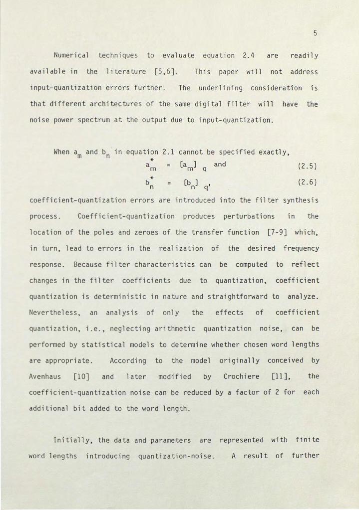
Numerical techniques to evaluate equation 2.4 are readily

available in the literature [5,6]. This paper will not address

input-quantization errors further. The underlining consideration is

that different architectures of the same digital filter will have the

noise power spectrum at the output due to input-quantization.

When a and b in equation 2.1 cannot be specified exactly, m n * a = [a ] and ( 2. 5) m m q

* (2.6) b = [b ] q' n n

coefficient-quantization errors are introduced into the filter synthesis

process. Coefficient-quantization produces perturbations in the

location of the poles and zeroes of the transfer function [7-9] which,

in turn, lead to errors in the realization of the desired frequency

response. Because filter characteristics can be computed to reflect

changes in the filter coefficients due to quantization, coefficient

quantization is deterministic in nature and straightforward to analyze.

Never t heless, an analysis of only the effects of coefficient

quantization, i.e., neglecting arithmetic quantization noise, can be

performed by statistical models to determine whether chosen word lengths

are appropriate. According to the model originally conceived by

Avenhaus [10] and later modified by Crochiere [11 J' the

coefficient-quantization noise can be reduced by a factor of 2 for each

additional bit added to the word length.

Initially, the data and parameters are represented with finite

word lengths introducing quantization-noise. A result of further

6

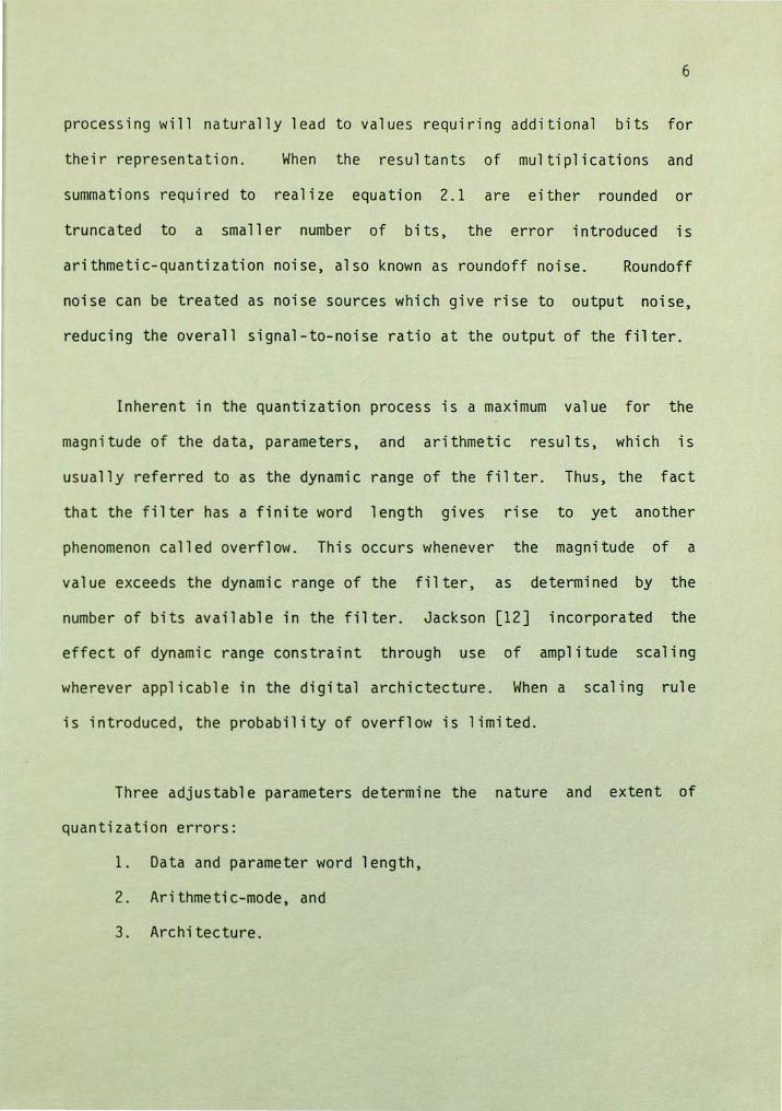
processing will naturally lead to values requiring additional bits for

their representation. When the resultants of multiplications and

summations required to realize equation 2.1 are either rounded or

truncated to a smaller number of bits, the error introduced is

arithmetic-quantization noise, also known as roundoff noise. Roundoff

noise can be treated as noise sources which give rise to output noise,

reducing the overall signal-to-noise ratio at the output of the filter.

Inherent in the quantization process is a maximum value for the

magnitude of the data, parameters, and arithmetic results, which is

usually referred to as the dynamic range of the filter. Thus, the fact

that the filter has a finite word length gives rise to yet another

phenomenon called overflow. This occurs whenever the magnitude of a

value exceeds the dynamic range of the filter, as determined by the

number of bits available in the filter. Jackson [12] incorporated the

effect of dynamic range constraint through use of amplitude scaling

wherever applicable in the digital archictecture. When a scaling rule

is introduced, the probability of overflow is limited.

Three adjustable parameters determine the nature and extent of

quantization errors:

1. Data and parameter word length,

2. Arithmetic-mode, and

3. Architecture.

7

Due to the limit on the word length available in mini-computers and

the desired word length in special purpose hardware systems,

quantization errors associated with finite coefficient word length

become a critical aspect of the design. All data and parameters within

the filter are quantized to a finite set of allowable values, with some

error incurred as a result of quantization. Word length limits the

dynamic range of the filter, and thus the realizable SNR. An erroneous

selection of the data and parameter word lengths may lead to a filter

that does not satisfy the original specifications of the filter. Since

the cost and complexity of the realization of the filter depends on

these word lengths, these should be kept to a minimum, but should be

sufficient to fulfill the performance requirements.

The most

floating-point.

commonly used arithmetic modes are

When two L-bit fixed-point numbers

fixed-point and

are added, their

sum would still have L-bits, provided there is no overflow. Therefore,

under this assumption, fixed-point addition introduces no errors; there

is, however, a dynamic range limitation because overflow is possible.

The product of two L-bit fixed-point numbers may have more than L-bits.

After rounding or truncating the results to L-bits, roundoff noise is

introduced into computations. On the other hand, floating-point is less

affected by the dynamic range constraint, but roundoff errors are

introduced during both additions and multiplications. Typically, the

arithmetic-quantization noise in a floating-point filter is less than

fixed-point filter with the same word length because of the automatic

8

scaling in a floating-point realization. Nevertheless, most

special-purpose digital filters have been constructed with fixed point

hardware because floating-point is more complex and costly to

implement.

Even more importantly, floating-point hardware is slower than

fixed-point hardware. Thus, floating-point arithmetic has a bandwidth

constraint which is undersirable in real-time processing applications

such as digital filtering.

There are three common ways of representing numbers in a fixed

point configuration: sign-magnitude, one 1 s complement, and two•s

complement. Once a word length is selected in any fixed-point

representation, the set representable numbers is fixed. If the word

length is L-bits (excluding the sign bit) and the numbers are normalized

such that lvl ~ 1, the smallest number variation that can be represented

-L is a 1 at the least significant register, which then corresponds to 2

Typically, the following two•s complement representation is selected

+00

I; - v ~ 0 L 2- k; v = where x = vk x, v < 0

k=l ( 2. 7)

because of finite register lengths, any number, v, must be approximated

by either rounding or truncating. Rounding can be effected by adding 1

at the position L + 1 and then truncating to L-bits. In truncating,

those bits beyond the most significant L-bits are simply dropped.

9

* Letting v be the machine representation of the result of either

rounding or truncating, then

L

x = L k=l

+ I

0

vL+l 2-L , round

, chop.

A convenient way of analyzing the effect of quantization is to represent

* the error e v - v, statistically. For the case of two's complement

fixed-point arithmetic, the error due to rounding and truncating is

represented as a random variable [13] with a uniform probability density

fun ct i on , p ( e ) , as sh own i n F i g u re 1 .

Since the error introduced by truncating is more serious than that

introduced by rounding, because of the bias shown in Figure 1,

truncating is not desirable.

Digital filter architectures are composed of three building

blocks: adders, constant multipliers and delays. Interconnection of

these elements into a particular architecture is a critical step in

filter syntheses. The architecture determines the spectrum of the

output noise and along with the arithmetic mode, determines the word

length required to satisfy the performance specifications.

TRUN CATI ON:

ROUNDING :

1

Q

- Q

1

Q

·- _q_ 2

10

0

0 _q_ 2

f i gure 1. Statistical Model of a Digital Multiplier

11

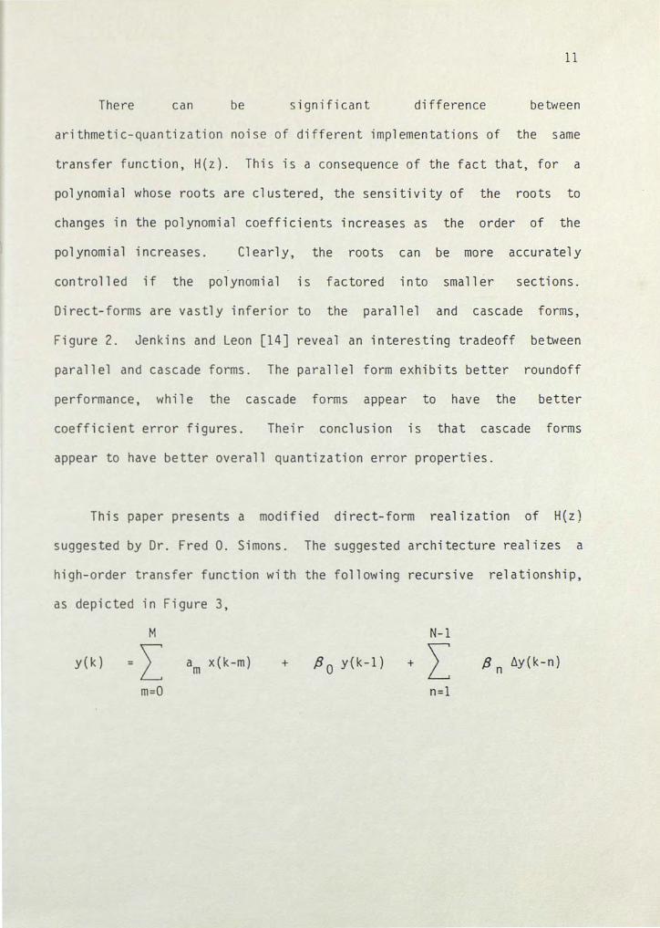
There can be significant difference between

arithmetic-quantization noise of different implementations of the same

transfer function, H(z). This is a consequence of the fact that, for a

polynomial whose roots are clustered, the sensitivity of the roots to

changes in the polynomial coefficients increases as the order of the

polynomial increases. Clearly, the roots can be more accurately

controlled if the polynomial is factored into smaller sections.

Direct-forms are vastly inferior to the parallel and cascade forms,

Figure 2. Jenkins and Leon [14] reveal an interesting tradeoff between

parallel and cascade forms. The parallel form exhibits better roundoff

performance, while the cascade forms appear to have the better

coefficient error figures. Their conclusion is that cascade forms

appear to have better overall quantization error properties.

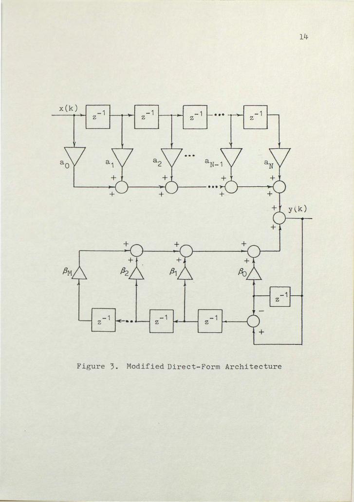
This paper presents a modified direct-form realization of H(z)

suggested by Dr. Fred 0. Simons. The suggested architecture realizes a

high-order transfer function with the following recursive relationship,

as depicted in Figure 3,

M

y(k) =L m=O

a x(k-m) m fJ tiy(k - n) n + p0

y{k-1)

n=l

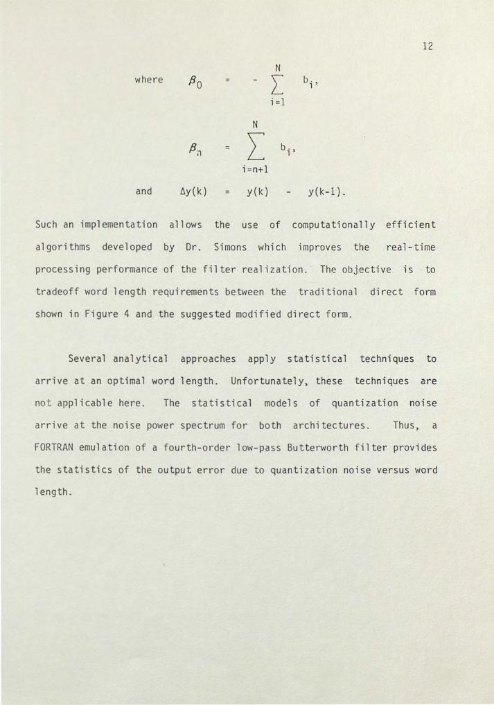
12

N where flo L bi)

i=l

N

fl;, L bi,

i=n+l

and 6y ( k) = y(k) y(k-1).

Such an implementation allows the use of computationally efficient

algorithms developed by Dr. Simons which improves the real-time

processing performance of the filter realization. The objective is to

tradeoff word length requirements between the traditional direct form

shown in Figure 4 and the suggested modified direct form.

Several analytical approaches apply statistical techniques to

arrive at an optimal word length. Unfortunately, these techniques are

no t applicable here. The statistical models of quantization noise

arrive at the noise power spectrum for both architectures. Thus, a

FORTRAN emulation of a fourth-order low-pass Butterworth filter provides

the statistics of the output error due to quantization noise versus word

length.

13

x ( z) y (z)

N

CASCADE FORM : H(z) = I1 C.(z) l

i=1

X(z) ~ c, c2 ..... C3 - ... B-Y(z) N

PARALLEL FORM : H(z) = 2= p. (z) l

i=1

p3 . . . .. .

I . .. . •

~1 PN

Figure 2 . Direct, Cascade , and Parallel Realizations

x(k)

-1 z

-1 z l---+-11......C -1 ••• z

...

..---···

-1 •• - z -1 z ~-~

-1 z

-1 z

Figure 3. Modified Direct-Form Architecture

14

x(k) +

+

• .. .

Figure 4.

-1 z

-1 z

-1 z

-1 z

. .

15

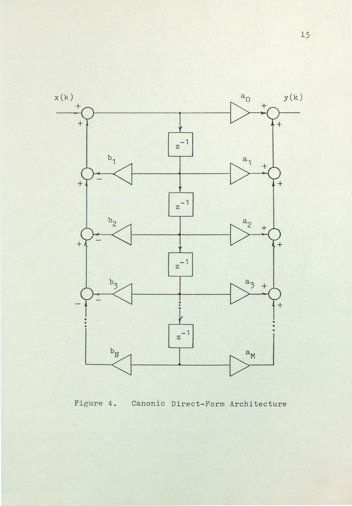
y(k)

Canonic Direct-Form Architecture

/

III. DEVELOPMENT OF REALIZATION SCHEMES

Modified Direct-Form

Given a high order transfer function of the following form

M

L -m m=O a z

H(z) m (3.1) N

1 L b -n + z n

n=l

we can arrive at the architecture previously described in equation 2.4.

Equation 3.1 implies the following input-output relationship:

[ M

l [ N

l L -m X(z) 1 L b z -n y ( z) . a z + m n

m=O n=l ( 3. 2)

Taking the inverse z-transform of both sides of equation 3.2, the

corresponding difference equation is available

M L am x(k-m)

m=O

y(k)

16

N

+ L bn y(k-n).

n=l

(3.3)

Solving for y(k),

M

y(k) =L m=O

a x(k-m) m

N

n=l

b y(k-n); n

17

(3.4)

a recursive relationship is otained which defines the current

output as a function of past outputs and present and past

Now, the objective is to modify the summation of weighted past

output values in equation 3.4 into a sum of weighted difference

operations.

Extracting from equation 3.4 the weighted sum of past output

values, we must arrive at the following expression

N N

L bn y(k-n) = L {3n b. y(k-n) ' (3.5)

n=l n=O

where l3n = f(bl, b2, bN)

and b.y ( k) = y ( k) y(k -1). (3.6)

Expanding the 1 ef t- hand side of equation 3.5,

N

L b y(k-n) n = bl y(k-1) + b2 y(k-2) +

n=l (3. 7)

+bN_ 2 y(k-N+2) + bN-l y(k-N+l) + bN y(k-N),

we can proceed to pair terms from n=N to n=l using difference

operators. The first pair of terms, n=N and n=N-1, can be

combined by adding underlined redundant terms, as follows:

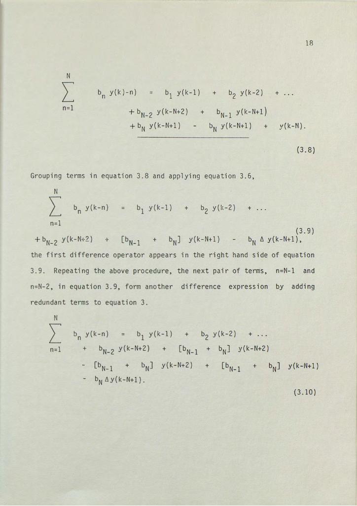
18

N

I b y(k)-n) n bl y(k-1) + b2 y(k-2) +

n=l + bN-Z y(k-N+2) + bN-l y(k-N+l}

+bN y(k-N+l) bN y(k-N+l) + y(k-N).

(3.8)

Grouping terms in equation 3.8 and applying equation 3.6,

N

I n=l

b y(k-n) n bl y(k-1) + b2 y(k-2) + ...

+ bN_ 2 y(k-N+2) + [bN-l + bN] y(k-N+l) (3.9)

bN /1 y(k-N+l),

the first difference operator appears in the right hand side of equation

3.9. Repeating the above procedure, the next pair of terms, n=N-1 and

n=N-2, in equation 3.9, form another difference expression by adding

redundant terms to equation 3.

N

~ bn y(k-n) b1 y(k-1) + b2 y(k-2) + ...

n=l + bN_ 2 y(k-N+2) + [bN-l + bN] y(k-N+2)

[bN-l + bN] y(k-N+2) + [bN-l + bN] y(k-N+l)

bN t1y(k-N+l).

(3.10)

19

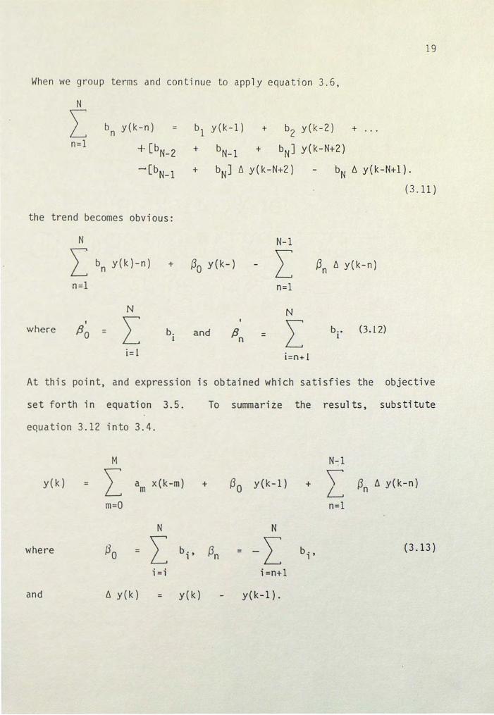
When we group terms and continue to apply equation 3.6,

N

L n=l

bn y(k-n) =

+ [bN-2

-[bN-1

the trend becomes obvious:

N

L b y(k)-n) + n

n=l

N I L where flo = b.

1

i= l

b1 y(k-1) + b2 y(k-2) + ...

+ bN-l + bN] y(k-N+2)

+ bN] 6 y(k-N+2) bN 6 y(k-N+l).

(3.11)

N-1

~o y(k-) L ~ tJ y(k-n) n

n=l

N

L and /Jn b .• (3. l 2)

= 1

i=n+ 1

At this point, and expression is obtained which satisfies the objective

set forth in equation 3.5. To summariie the results, substitute

equation 3.12 into 3.4.

M N-:1

y(k) L a x(k-m) + ~o y(k-1) + \ ~ 6 y(k-n) m L n

m=O n=l

N N

where f3o = L bi, ~n = -L bi, (3.13)

i =i i=n+l

and /j y ( k ) = y(k) y(k-1).

Canonic Direct-Form

A digital network is said to be "canonic" if the number of unit

delays employed is equal to the order of the transfer function, H(z).

The computational algorithms to realize such a canonic form are derived

from

H(z)

in the following paragraphs.

Y(z) X{Z)

M

L m=O

1 -n z

(3.14)

An intermediate variable, W(z), can be introduced by partitioning

equation 3.14

H(z) =[~] W(z)

The first term,

N(z)

[~] X(z)

Y(z)

W(z)

20

N(z)

M

a

m=O

m

[D(:J .

-m z

(3.15)

(3.16)

leads to

M

Y(z) =I m=O

or equivalently,

M

y(k) I m=O

in the time domain. Similarly, the

1 W(z) O(z) X(z)

1 eads to

W(z) = X(z)

or equivalently,

w(k) x(k)

-m a z W(z); m

a m

second

1 +

N

I n=l

N

I n=l

w(k-m)

term,

1

N

I b -n z n

n=l

b -n w ( z); z n

b w(k-n). n

21

(3.17)

(3.18)

(3.19)

(3.20)

(3.21)

22

Therefore, in place of equation 3.4, we have the following

computational algorithms:

N

w(k) :::: x(k) l>n w(k-n) (3.22)

n==l

and

M

y(k) =L a w(k-m). m (3.23)

m==O

Equation 3.22-3.23 represent the digital architecture depicted in

Figure 4.

IV. EMULATION OF DIGITAL PROCESSES

In two's complement fixe d-point arithmetic, we assume that a

* quantity y is approximated by y as follows:

-F * y

I ~ x

' y > 0 * L y

I+ l where x = Y. F 21

* l + + l ( 4. 1) 2 y x, y < 0 y 1= I -1 y

and are binary digits taking values 0, 1. The

sign bit, yN, denotes a positive value if equal to zero and negative

value if equal to one.

Considering the previous definition, the numerical system can be

defined with the following scaling rule:

and s y

I y

F y

nd N

sign bit,

= number of

number of

I + F + 1 y y

(refer to Figure 5) .

s I F (4.2) y y y

integer bits,

fractional bi ts,

the total number of bits per binary word

23

24

Using this notation, we can examine hovJ to emulate the only two

operations required to realize a digital filter: summation and

multiplication.

* Given y, with its corresponding finite register representation y ,

the objective is to emulate the effect of quantization in a numerical

system specified by s y I y

The quantization process is

accomplished by efther truncating or rounding. The truncation, or

chopping effect, can be emulated by the following expression:

* y = -F

2 y F

INT (2 Y. y) (4.3)

where INT ( ) is a function that truncates the fractional part of a real

number in FORTRAN and BASIC. Rounding is accomplished by adding the

weigh~of the most significant bit of the discarded parts of the

fraction. In order to emulate this effect, the following rule is

applicable: -F -(F + 1)

YR = YT + 2 y, if y - y < 2 y T

(4.4) = YT otherwise;

where y = the exact quanity,

* y = truncated N bi ts,

y = y rounded to N bits,

* and F = number of fractional bi ts y y

25

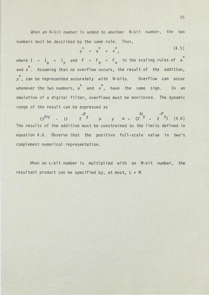
\~hen an N-bit number is added to another N-bit number, the two

numbers must be described by the same rule. Thus,

* * * y = a + x , (4.5)

* where I I a and F = F x in the scaling rules of a

* and x . Assuming that no overflow occurs, the result of the addition,

* y , can be represented accurately with N-bits. Overflow can occur

* * whenever the two numbers, a and x , have the same sign. In an

emulation of a digital filter, overflows must be monitored. The dynamic

range of the result can be expressed as

l) -F

2 y y N -F

~ - (2 y • 2 Y) (4.6)

The results of the addition must be constrained to the limits defined in

equation 4.6. Observe that the positive full-scale value in two's

complement numerical representation.

When an L-bit number is multiplied with an M-bit number, the

resultant product can be specified by, at most, L + M.

* *

*

*

* *

*

*

I ~ I

I-~ Iy •t"

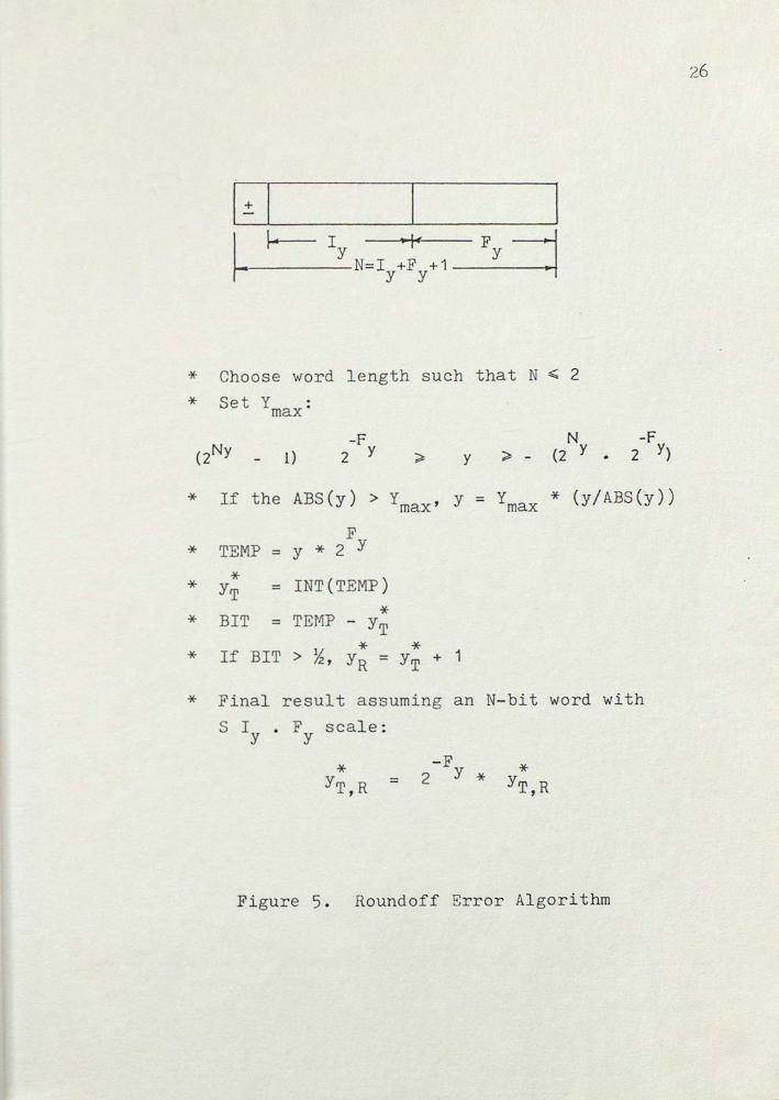
i--------N=I +F +1 y y

Choose word length such that N ~ 2

Set ymax=

l) -F

2 y y N -F

~ - (2 y • 2 Y)

If the ABS(y) > Y max' y = ymax * (y/ABS(y))

F TEMP = y * 2 y

* YT = INT(TEMP)

* BIT = TEMP - yT

* * If BIT > ~' YR = YT + 1

Final result assuming an N-bit word with

S Iy • FY scale:

-F = 2 y *

Figure 5. Roundoff .Error Algorithm

26

In this case,

* y * * a x ,

27

( 4. 7)

where the resultant scalilng rule with the double precision accuracy is

+ + Fx) (4.8)

given the scaling rule of the factors S I a a F and S Ix a x

Observe the result has two sign bits; their value conforms to the normal

algebraic rules pertaining to positive and negative factors. The

roundoff error is introduced into the computations when the result must

be stored in an N-bit word if N L+M. This single-precision computation

can be modeled by applying equation 4.3.

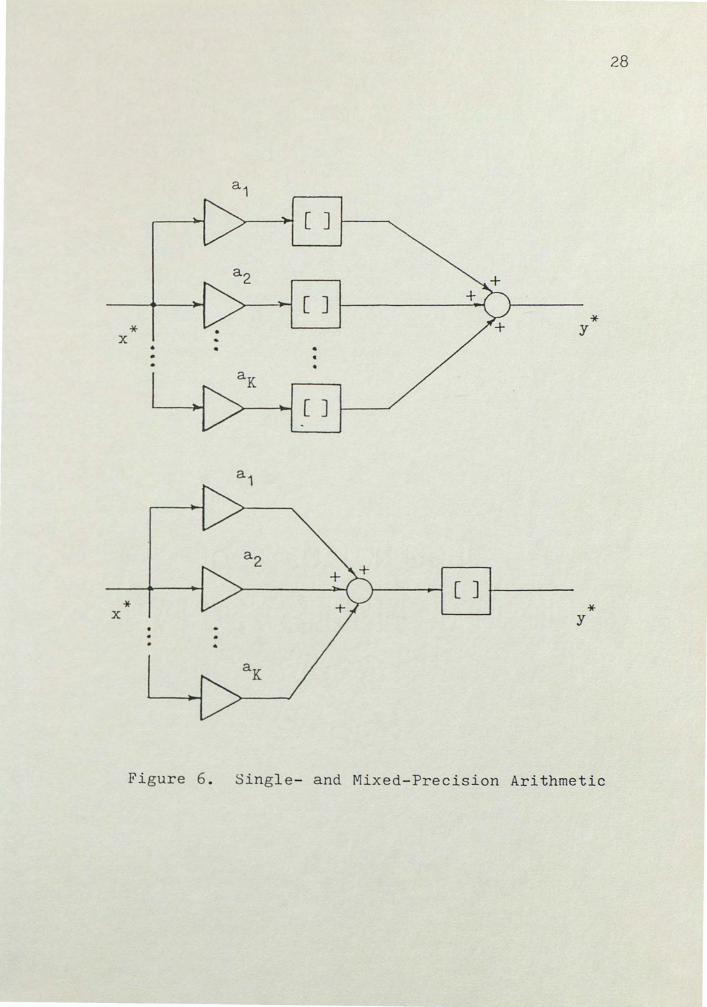
In digital signal processing applications, the sum of K products

K

* L * y = a.x l

(4.9)

i =i

is encountered frequently (see Appendix). These can be computed in

single-precision, i.e., by summing quantized results, or in mixed

precision, by quantizing only the final result, Figure 6.

28

[ J

[ J * * • y

x • • .

I

[ J

a2

[ J * * x y

• . . aK

Figure 6. Single- and Mixed-Precision Arithmetic

29

By quantizing the result only once, the arithmetic roundoff error

is decreased by a factor K; and hence the digital process is more

accurate by using mixed-precision arithmetic.

An emulation of any digital process can be carried out with a

general purpose computer using equations 4.3, 4.4, 4.5, and 4.8. These

provide adequate models for truncation, rounding,

constraints and summation of products.

dynamic range

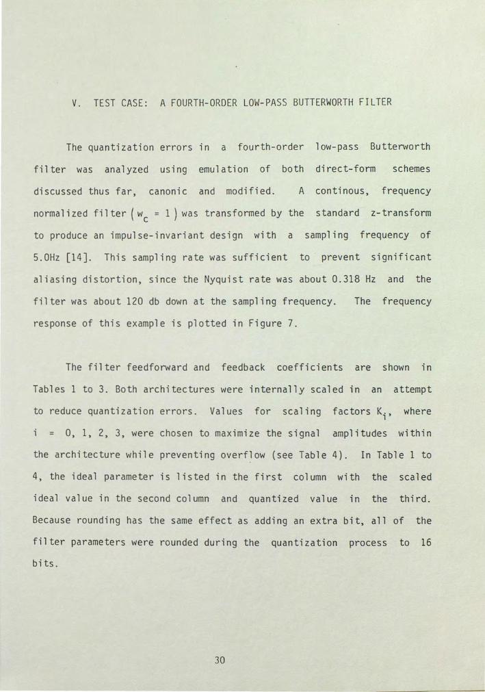
V. TEST CASE: A FOURTH-ORDER LOW-PASS BUTTERWORTH FILTER

The quantization errors in a fourth-order low-pass Butten~orth

filter was analyzed using emulation of both direct-form schemes

discussed thus far, canonic and modified. A continous, frequency

normalized filter ( wc = 1) was transformed by the standard z-transform

to produce an impulse-invariant design with a sampling frequency of

5.0Hz [14]. This sampling rate was sufficient to prevent significant

aliasing distortion, since the Nyquist rate was about 0.318 Hz and the

filter was about 120 db down at the sampling frequency.

response of this example is plotted in Figure 7.

The frequency

The filter feedforward and feedback coefficients are shown in

Tables 1 to 3. Both architectures were internally scaled in an attempt

to reduce quantization errors. Values for scaling factors Ki' where

= 0, 1, 2, 3, were chosen to maximize the signal amplitudes within

the architecture while preventing overflow (see Table 4). In Table 1 to

4, the ideal parameter is listed in the first column with the scaled

ideal value in the second column and quantized value in the third.

Because rounding has the same effect as adding an extra bit, all of the

filter parameters were rounded during the quantization process to 16

bits.

30

31

JH(z)I, db

0

-10

-20

-30

-40

0 • 1 .2 .3 .4 . 5

Frequency, Hz

Figure 7. Frequency Response of the Fourth-Order

Low-Pass Butterworth Digital Filter

rn

0 I 2 3

n

1 2 3 4

n

0 I 2 3

32

r I\ I\ I. I i

FU : I )I · { rn WI\ JU) C: OEFFIC 11.'..NT.)

cl m

a /K m 0

a rn R

0.0 1.167999769 3 37 80 4.09288249892140 0.89945265957342

0.0 0.13960004334517 0.66439285312713 0.14600710352771

TABLE 2

0.0 0.18960571289063 0.66439819335938 0.14 59960937 5000

FEEDBACK COEFFlCIENTS OF CANONIC DIRECT-FORM

b bn/K I b [bn/K 1) n n

-3.46881512365680 -0.4348.5189045710 -0.4 34 84497070313 4.56797554873600 0.57099694359200 0.5709838867187 5

-2.6808902285908 0 -0.33511127857385 -0.33508300781250 0.59261867788150 0.07412023347352 0.07412719726563

TABLE 3

FEEDBACK COEFFICIENTS OF THE MODIFIED DIRECT-FORM

o. 9987679 3572 34 5 2.48007187187933

- 2.08792836080265 0.59296186778815

K. I

0 6.1603 3492783262

8.0

2 4.0

0.24969198393086 0.6200 l I 796983 34

- 0.52198209020066 0.14825439453125

Tl\l\LE 4

')CALIN(. Pl\Rl\METER\

3 1.232064276549980-3

0.2496948242187 5 0.62002563476563

- 0.52197265625000 0.14824046694 704

Description

M

L a m

m=O

max(b ) n

mod 2

max( pn ) mod 2

N

1 .. L b n

n=I

R

R

33

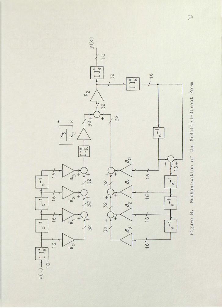
In the mechanization of both computational algorithms, word

lengths and scaling rules are shown in Figures 8 and 9. The assumption

is that a 16Xl6 parallel multiplier accumulator (see Appendix) is used

to carry out the hardware realization.

Using the techniques presented in Chapter IV, an emulation of the

architectures was carried out. The statistics of the output noise,

e(k) y true

y true

where Yt is the ideal response rue and Y f i l ter

response, were computed for a step input,

0.5, k ~ 0

x(k) =

0.0, k < 0

All internal states were in i ti a 1 i zed to zero.

. 2 computed with the following variance, a , were e

N samp

m 1 L e

k + 1 k=O

N samp

02 1 L = ·e

k + 1 k=O

(5 . 1)

is the actual filter

(5.2)

The mean, me' and the

equations:

e(k) (5.3)

[e(k) m ] 2 e

( 5. 4)

x(k

)

16

-1

z -1

z

-1 ,

, >

<

(

z

Fig

ure

8

. M

ech

aniz

atio

n

of

the

Mo

dif

ied

-Dir

ect

Form

\...

..-.)

~

x(k

)

[ J * R

*

[ :: L

1

6

\.

,)

" '-..

....

I

32 '-

l

1 6

-1

z I'-

16

---,

I

z -1

-1

z

-1

z 16

1 6

16

Fig

ure

9.

M

ech

aniz

atio

n

of

the

Can

on

ic

Dir

ect-

Fo

rm

y(k

) ~

10

\..,..

.) \)\

36

where N was selected empirically as 100 samples. After 100 samples samp

of the output, the output of the ideal filter settles out within z- 9 of

the actual filter. Observe that the D/A of the filter output was

assumed to be 10 bits (including sign bit). In digital signal

processing of analog signals, the quantization error is commonly viewed

as additive noise signal. The ratio of the signal-to-noise power (SNR)

is a useful measure of the relative strength of the signal and the

noise. A common rule of thumb, derived from the statistical models

discussed in Chapter II, is that the signal-to-noise ratio increased

approximately 6 db with each additional bit. Thus,

SNR = 6L

where L is equal to the word length sign bit. For the fourth -o rder

low-pass filter, a SNR of 54 db is adequate.

The results of the emulation are summarized in Tables 5 and 6. In

Table 5, the statistics of the following noise sources are shown:

a) etot' output noise as defined by equation 4.1;

b) eR, noise due only to roundoff of computations;

c) e~~+ eR, noise due to roundoff and quantization of

feedback coefficients; and

d) ea + eR, noise due to roundoff and quantization of

feedforward coefficients.

37

TABLE 5

ST A TIS TICS ON NOISE SOURCES

Noise Source Modified-Direct Form Canonic-Direct Form

2 2 2 2 2 2 m (j m + (j m (j m + (j

e e e e e e e e

etot 0.0502 0.0191 0.0216 O. l 383 0.0205 0.0396

eR 0.0499 0.0191 0.0216 0.0195 0.0200 0.0204

eb,/J + eR 0.0569 0.0188 0.0220 0.1383 0.0200 0.0396

ea + eR 0.0569 0.0188 0.0220 0.0195 0.0200 0.0204

TABLE 6

STA TlSTICS ON e VERSUS WORD LENGTH tot

Word Length Modified-Direct Form Canonic-Direct Form

m 2 2 2 2 2 2 e (j m + <1 m <1 m + <1 e e e e e e e

18 0.0293 0.0197 0.0205 0.0804 0.0188 0.0253

17 0 .0356 0.0195 0.0208 0.1385 0.0200 0.0392

16 0.0502 0.0190 0.0216 0.1383 0.0205 0.0396

15 0.0907 0.0189 0.0271 0.1391 0.0198 0.0391

14 0.0635 0.0241 0.0282 0.3135 0.0333 0.1316

38

In Table 6, the s tatistic s of were gathered \Ali th

perturbations of the word length. Because of the architectures used

parallel multiplier.-accumulator, as the single-precision word length, L

was varied the mixed-precision word length of the accumulator was also

varied accordingly (see Appendix). Also included in Tables 5 and 6 is

m2 +J, the total noise power. Using m, a 2, and m 2 +a 2 as figures e e e e

of merit, a comparison of the direct forms is possible.

From Table 5, several qualitative and quantitative conclusions can

be drawn. The canonic direct-form is much more sensitive to

quantization noise than roundoff noise. On the other hand, the

suggested modified direct from exhibits the opposite trend; it is more

susceptible to roundoff noise. Another obvious result is a 50%

reduction in the noise level in the modified direct-form versus the

canonic direct-form.

From Table 6, an inter~sting trend is presented. The canonic

direct-form is more sensitive to perturbations of the word length. By

adding two additional bits, a reduction of 35% in the noise power is

apparent comparable to the suggested direct-form baseline.

Although the results appear to indicate that the over a 11

performance of the modified direct-form surpasses that of the canonic

for~, there are several drawbacks inherent to the suggested direct-form.

For instance, more double-precision computations are required to

implement the suggested direct-form and twice as many delays (memory

39

locations) are also required in the modified direct-form realization.

Like in any other synthesis and de s ign problem, a tradeoff is introduced

with new alternatives.

VI. CONCLUSION

As the capabilities of digital components continue to grow while

their cost drops , digital signal processing has become more attrative

than analog circuitry for many applications. In the filtering area of

signal processing, digital filters are replacing their analog

counterparts because digital filters do not drift with temperature or

voltage, require less maintenance or calibration, and have almost no

limit on the possible signal-to-noise ratio assuming adequate word

length. Moreover, one fast digital filter can be timeshared between

many independent inputs, giving it even more useful channel-bandwidth

capability. This circuit can also be precisely simulated, and easily,

exactly repeated. The advantages and applications are many.

Despite the many advantages provided by digital filtering

techniques, there is an inherent limitation on the performance of these

filters, due to the effects of finite word length. There is an infinite

variety of network implementations that realize a given transfer

function when the parameters are represented with infinite accuracy. It

is to be expected that some of these architectures will be less

sensitive than others to quantization noise, i.e., the transfer function

of the resulting realization approach to the desired function.

For realizing the transfer function as a computer program or in

hardware, a digital architecture must be chosen such that quantization

40

41

effects are minimal. There are many other considerations such as

implied hardware or software complexity and difficulty in determining

parameters of the filters . Unfortunately, no systematic approach has

been developed to determine an optimal realization in terms of the

typical constraints: number of multipliers, word length, and memory

allocation.

In this paper, two direct-form realizations were examined.

Instead of a detailed mathematical analysis of the parameter

sensitivity, a more direct approach was taken. By using an emulation of

both architectures, a comparison of performance was possible. The

suggested modified direct-form did prove to be less sensitive to

quantization noise. The empirical results show a 50% reduction of the

noise level in the modified direct-form versus the canonic direct-form.

In spite of its inherent drawbacks, this architecture merits further

study.

APPENDIX: THE PARALLEL MULTIPLIER-ACCUMULATOR

An element of critical importance in the hardware realization of a

digital filter is the multiplier, which is required to produce the

product of a filter parameter and a digital signal. The multiplication

operation requires complex circuitry and is the principal controlling

factor in the processing rate and the power consumption of the fil t er.

Due in part to its importance in digital filters, considerable attention

has been devoted to research and development of both multiplication

algorithms and multiplier circuits.

A series of monolithic parallel

by TRW are capable of performing

multipler-accumulators developed

8X8-, 12Xl2-, or 16Xl6- bit

multiplication and the accumulation of product terms with the contents

of an putput register. Mac-8, -12, and -16 are informal ways of

referring to the TDC1008J, TDC1009J, and TDClOlOJ and their handling of

8-, 12-, and 16- bit word [15]. These are high performance, TTL

compatible devices fabricated in a bipolar VLSI technology which can be

employed as the central building block of a digital filter. A

functional diagram of such a device is shown in Figure 10, showing the

pair of clocked input registers, followed by the multiplier,

accumulator, and clocked output registers and the three-state output

buffers [16].

42

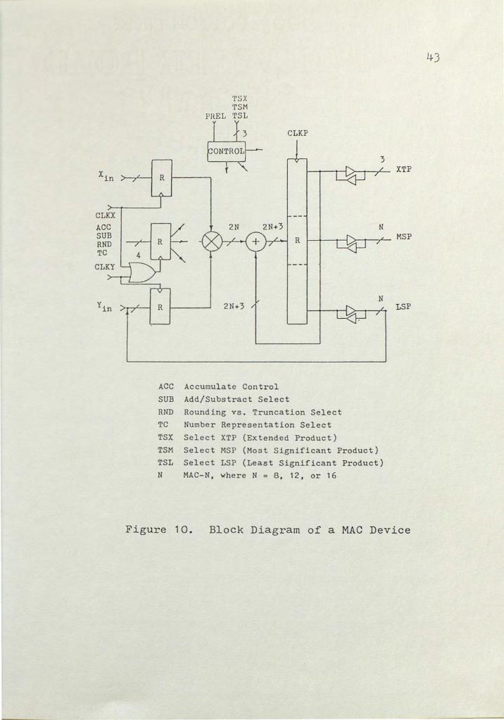
CLKX

ACC SUB RND TC

'l'SX ·rsM

PREL ·rs1

rON~R~ - CLKP

R

R 2N+3

ACC Accumulate Control

SUB Add/Substract Select

R

RND Rounding vs. Truncation Select

TC Number Representation Select

TSX Select XTP (Extended Product)

3

N

N

TSM Select MSP (Most Significant Product)

TSL Select LSP (Least Significant Product)

N MAC-N, where N = 8, 12, or 16

XTP

MSP

LSP

Figure 10. Block Diagram of a MAC Device

43

44

The three most critical characteristics of a multiplier are speed

of multiplication, power dissipation, and word length. These devices

are very fast, with a multiply-accumulate time of 70 nanoseconds for

Mac-8, 95 nanoseconds of Mac-12, and 115 nanoseconds for Mac-16. Power

consumption from a single 5 volt source is moderate (1.2 watts for

Mac-8, 2.5 watts for Mac-12, and 3.5 watts for Mac-16) [16].

Other features of secondary importance are expandability, data

representation, and rounding. Expandability refers to building of l arge

multipler arrays for several multipliers. The TRW is non-expandable;

but pipelining is an acceptable solution to obtain high speed

multiplication of words greater than 16- bits in length [17]. Data

representation is either unsigned or signed (two's complement); this is

a selectable function in the TRW series.

Rounding is useful when a single-length product is desired. This

is accomplished by raising the rounding pin to logic one, which

propagates a carry into the least significant bit (of the single length

product) if the most significant bit of the lower half is one, see

Figure 10.

Devices like the TRW MAC series are being used to

real-time capability of the microprocessor systems.

microprocessor is left to perform the basic tasks of memory

upgrade the

While the

management

and control, the MAC does the "number crunching" operations at a data

speed order of a magnitude higher than possible in the microprocessor

LIST OF REFERENCES

1. J.F. Kaiser, "Some Practical Considerations in the Realizations of Linear Digital Filters," Proceedings 3rd Annual Allerton Conference Circuit and System Theory, (Monticello, Ill.), pp. 621-633, October 1965.

2.

3.

J.B Knowles and E.M. Olcayto, "Coefficient Accuracy and Fi 1 te r Response , 11 I EE E Trans act i on s Ci r cu i t Theory, Vo 1 . No. 2, March 1968, pp. 31-41. Reprinted by IEEE in [19].

Di gi ta 1 CT-15,

Bede Lieu, "Effect of Finite Word Length on Digital Filters -- a Review, 11 IEEE Transactions Vol. CT-18, No. 6, November 1971, pp. 670-671.

the Accuracy of Circuit Theory,

4. Athanasios Papoulis, Probability, Random Variable and Stochastic Processes. New York, NY: McGraw-Hill Book Company, 1965.

5. Sajit K. Mitra, Kotaro Hirano, and Hisashi Sakaguchi, "A Simple Method for Computing the Input Quantization and Multiplication Roundoff Errors in a Digital Filter, 11 IEEE Transactions Acoustic, · Speech, and Signal Processings, Vol. ASSP-22, No. 5, October 1974.

6. K.J. Astrom, E.J. Jury, and Roger G. Agni el, "A Numerical Method for the Evaluation of Complex Integrals, 11 IEEE Transactions Automatic Control, August 1970.

7. Andreas Antoniou, Digital Filters: Analysis and Design. New York, NY: McGraw-Hill Book Company, 1979.

8. Alan V. Oppenheim and Ronald W. Schafer, Digital Signal Process­ing. Englew9od Cliffs, NJ: Prentice-Hall, 1975.

9. Lawrence R. Rabiner and Bernard Gold, Theory and Application of Digital Signal Processing. Englewood C~l~i~ff~s~,---.,.N~J~:--~P~r_e_n~t~i-c-e~-H~a~l~l~,

1975.

10. Ernst Avenhaus, "On the Design of Digital Filters with Coefficients of Limited Word Length," IEEE Transactions Audio Electroacoustics, Vol. AU-20, No. 3, August 1972, pp. 206-212. Reprinted by IEEE in [19].

45

46

11. R.E. Croochiere, "A New Statistical Approach to the Coefficient Word Length Problem for Digital Filters," IEEE Transactions Circuits and Systems, Vol. CAS-22, No. 3, March 1975, pp. 190-196. Reprinted by IEEE in [19].

12. Leland B. Jackson, "On the Interaction of Roundoff Noise and Dynamic Range in Digital Filters, 11 The Bell System Technical Journal, Vol. 49, No. 2, February 1970, pp. 159-183.

13. A.V. Oppenheim and C.J. Weinstein, "Effects of Finite Register Length in Digital Filtering and the Fast Fourier Transform," Proceedings IEEE, Vol. 60, No. 8, pp. 957-976.

14. W.K. Jenkings and B.J. Leon, "An Analysis of Quantization Errors in Digital Filters Based on Interval Algebras." IEEE Transactions Circuits and Systems, Vol. CAS-22, No. 3, March 1975.

15. Louis Schirm IV, "Packing a Signal Processor Onto a Single Digital Board," Electronics, December 20, 1979.

16. TRW, Inc., MPY-Series Multipliers. Redondo Beach, CA: TRW, Inc., October 1977.

17. TRW, Inc., LSI Multipliers Application Notes. LaJolla, CA: TRW, Inc. 1982.

18. Shlomo Waser,"High Speed Monolithic Multipliers for Real-Time Digital Processing," IEEE Transactions Electronic Computers, October 1978.

19. Digital Processing Committee. Papers in Digital Signal Processing II. New York: IEEE Press, 1975.