
Effects of errors in flutter derivatives on the wind ...811/fulltext.pdfEFFECTS OF ERRORS IN FLUTTER...
187
EFFECTS OF ERRORS IN FLUTTER DERIVATIVES ON THE WIND- INDUCED RESPONSE OF CABLE-SUPPORTED BRIDGES A Dissertation Presented by Dong-Woo Seo to The Department of Civil and Environmental Engineering in partial fulfillment of the requirements for the degree of Doctor of Philosophy in Civil Engineering in the field of Structural Engineering Northeastern University Boston, Massachusetts February 2013
Transcript of Effects of errors in flutter derivatives on the wind ...811/fulltext.pdfEFFECTS OF ERRORS IN FLUTTER...

EFFECTS OF ERRORS IN FLUTTER DERIVATIVES ON THE WIND-INDUCED RESPONSE OF CABLE-SUPPORTED BRIDGES
A Dissertation Presented
by
Dong-Woo Seo
to
The Department of Civil and Environmental Engineering
in partial fulfillment of the requirements
for the degree of
Doctor of Philosophy
in
Civil Engineering
in the field of
Structural Engineering
Northeastern University
Boston, Massachusetts
February 2013
ii
Abstract
This dissertation discusses the development and implementation of a methodology for the
buffeting response of cable-supported bridges, including uncertainty in the aeroelastic input
(i.e., flutter derivatives, FDs). Flutter derivatives are the most important part of the loading
and are estimated in a wind tunnel experiment.
A second order polynomial model (“model curve”) for the flutter derivatives is
proposed. The coefficients of this polynomial are random variables, whose probability
distribution is conditional on the reduced wind speed. For computational reasons in
subsequent analysis, however, this dependency is neglected and the probability of these
random variables is treated as independent of the reduced wind speed. For analysis purposes
the first- and second-order statistics are estimated from experiments, treating all the wind
speed data as part of the same population. Wind tunnel experiments are conducted at
Northeastern University and a section model of a truss-type bridge deck is used.
The simplified polynomial model for the FDs, including the second order description
of its variability, is employed in the derivation of the probability of the onset of flutter using
Monte-Carlo (MC) simulations.
The simplified stochastic “model curves” for FDs are used to estimate the buffeting
bridge response. In the standard approach the result of the buffeting analysis is the value of
the RMS dynamic response at a given wind speed. In the proposed probabilistic setting one

iii
estimates the probability that a given threshold for the variance of the response is exceeded.
This probability is later used, together with information on the probability of the wind
velocity at a given site, to predict the expected value of the loss function due to the buffeting
response of a 1200-meter suspension bridge (a function proportional to the cost associated
with interventions needed to ensure safety).

iv
Acknowledgments
I would like to most sincerely thank my advisor Dr. Luca Caracoglia for his constant
guidance, teaching, and support throughout this rather complicated and intense research. He
has motivated and encouraged me towards improvement and excellence in research. I have
been grateful to work with him and to be part of his research team.
I would also like to thank my PhD committee members, Professor George G. Adams,
Professor Dionisio P. Bernal and Professor Mehrdad Sasani for their overall encouragement
through the PhD studies and for valuable comments and recommendations.
The PhD studies, described by this research, were supported in part by the National
Science Foundation of the United States (NSF), Award No. 0600575 from 2008 to 2010.
Any opinions, findings, conclusions and recommendations are those of the writer and do not
necessarily reflect the views of the NSF. The Department of Civil and Environmental
Engineering is also acknowledged for providing support from 2010 until the completion of
the program in the form of teaching assistantship.
Finally, I am deeply grateful to my parents and younger brother, whose love and
support has always been a tremendous source of strength and encouragement for me. They
never lost faith in me and are always willing to provide a helping hand. Their love and
invaluable support gave me the motivation to accomplish many goals in my life.

v
Table of Contents
Abstract ii
Acknowledgments ................................................................................................................. iv
Table of Contents ................................................................................................................... v
List of Tables ...................................................................................................................... viii
List of Figures ....................................................................................................................... ix
Nomenclature ..................................................................................................................... xiii
Chapter 1 1
Introduction ........................................................................................................................ 1
1.1 Motivation .................................................................................................................... 4
1.2 Outline .......................................................................................................................... 6
Chapter 2 9
Wind-Induced Response of Long-Span Bridges: Review .................................................. 9
2.1 General Formulation .................................................................................................... 9
2.2 Background on Flutter ............................................................................................... 18
2.3 Background on Buffeting ........................................................................................... 20
2.4 Effect of Wind Directionality: Skew Wind Theory .................................................... 27
Chapter 3 31
A Second-order Polynomial Model for Flutter Derivatives ............................................. 31
3.1 Description of the Polynomial Model and Discussion on its Physical Interpretation 32
3.1.1 Description of the Polynomial Model ................................................................. 32
3.1.2 Discussion on the Selection of the Polynomial Model, based on Physical Behavior of Flutter Derivatives ................................................................................................... 33
3.2 Description of the Wind Tunnel, used for Experimental Verification of the Polynomial Model ............................................................................................................................... 35
3.3 Description of the Experimental setups, used for Verification .................................. 36
3.4 Description of the Aeroelastic Section-Model, used for Verification ........................ 37

vi
3.5 Description of the Tests and Experimental Identification .......................................... 38
3.6 Reason for the Use of the Polynomial Model in the Context of Random Flutter Derivatives ....................................................................................................................... 41
3.6.1 Estimation of Variance and Co-variance of Cj and Dj coefficients of the “Model Cures” from Experiments ............................................................................................. 43
3.7 Summary of Experimental Results and Comparison with Literature Data (“Jain’s Data”) ............................................................................................................................... 46
Chapter 4 58
A Methodology for the Analysis of Long-Span Bridge Buffeting Response, accounting for Variability in Flutter Derivatives ...................................................................................... 58
4.1 Introduction ................................................................................................................ 58
4.2 Multi-Mode Buffeting Analysis (“Deterministic Case”) ........................................... 60
4.2.1 Validation for Closed-Form Solution .................................................................. 61
4.2.2 Monte-Carlo and Quasi-Monte-Carlo Methods .................................................. 62
4.2.3 Examination of the Computational Efficiency of the MC and QMC Methods for Calculating the Double Integral in Eq. (2.24) .............................................................. 64
4.3 Monte-Carlo-based Methodology for Buffeting Analysis Considering Uncertainty in the Flutter Derivative (“Statistical Case”)........................................................................ 68
4.3.1 Description of the Bridge Example and RMS Threshold Levels (“Probabilistic Setting”) ....................................................................................................................... 72
4.3.2 TEP Curves using Literature Data ...................................................................... 73
4.3.3 TEP Curves using NEU’s Flutter Derivative Data .............................................. 77
4.4 Effect of Wind Directionality on “Statistical Buffeting” Response: TEP Surfaces ... 78
4.5 Exploratory Performance Analysis on a Full-Scale Structure.................................... 79
4.6 Summary .................................................................................................................... 81
Chapter 5 120
Lifetime Cost Analysis due to Buffeting Response on a Long-Span Bridge, accounting for Variability in Flutter Derivatives .................................................................................... 120
5.1 Introduction .............................................................................................................. 120
5.2 Peak Estimation via RMS Response ........................................................................ 121
5.3 Lifetime Expected Cost Analysis ............................................................................. 122
5.4 Description of the Structural and Aeroelastic Model ............................................... 126
vii
5.5 Estimation of Peak Dynamic Response during Buffeting ........................................ 127
5.6 Monte-Carlo-based Methodology for “Statistical Buffeting” Analysis considering Uncertainty in the FD ..................................................................................................... 128
5.6.1 Wind-Direction-Independent Analysis .............................................................. 128
5.6.2 Wind-Direction-Dependent Analysis ................................................................ 129
5.7 Flutter Analysis: Numerical Results ........................................................................ 130
5.8 Lifetime Expected Intervention Cost Analysis - Numerical Results ....................... 132
5.8.1 Estimation of the Limit-State Probabilities Pj from TEP Analysis ................... 132
5.8.2 Expected Intervention Cost - Description of the Simulations ........................... 134
5.8.3 Expected Intervention Cost - Numerical Results using NEU’s FD Data.......... 135
5.9 Discussion and Remarks .......................................................................................... 135
Chapter 6 158
Summary and Conclusions ............................................................................................. 158
6.1 Summary .................................................................................................................. 158
6.2 Conclusions .............................................................................................................. 160
6.3 Recommendations for Future Research ................................................................... 161
6.4 Outcome of the PhD Studies: List of Deliverables .................................................. 162
6.4.1 Journal Publications (Published/under review) ................................................. 162
6.4.2 Other Journal Publications (not related to the main topic of this Dissertation) .. ...................................................................................................................... 163
6.4.3 Full Papers in Conference Proceedings............................................................. 163
6.4.4 Other Papers Published as Conference Proceedings (not related to the main topic of the Dissertation) ..................................................................................................... 163
6.4.5 Poster Presentations .......................................................................................... 164
References .......................................................................................................................... 165

viii
List of Tables
Table 3.1 The static coefficients and their derivatives at α0 (Jain et al., 1998). ................... 48
Table 4.1 Natural frequencies and mode types of Golden Gate Bridge (Jain 1996). ........... 83
Table 4.2 Comparison of closed-form numerical solution with literature results at l/4. ...... 83
Table 4.3 Bias and relative errors in the MC case: (a) for heave σhh; (b) for torsion σαα. .... 84
Table 4.4 Bias and relative errors in the QMC case: (a) for heave σhh; (b) for torsion σαα. . 85
Table 4.5 Threshold values for σhh and σαα, employed in the TEP analysis with flutter derivatives from the literature. ............................................................................ 86
Table 4.6 Study cases used for serviceability on full-scale structure. .................................. 86
Table 5.1 Structural performance thresholds for vertical deck response (Tj). .................... 137
Table 5.2 Probabilities of each damage state (Pj) due to buffeting response based on the structural performance thresholds (T = Tj) using NEU’s FD data..................... 137

ix
List of Figures
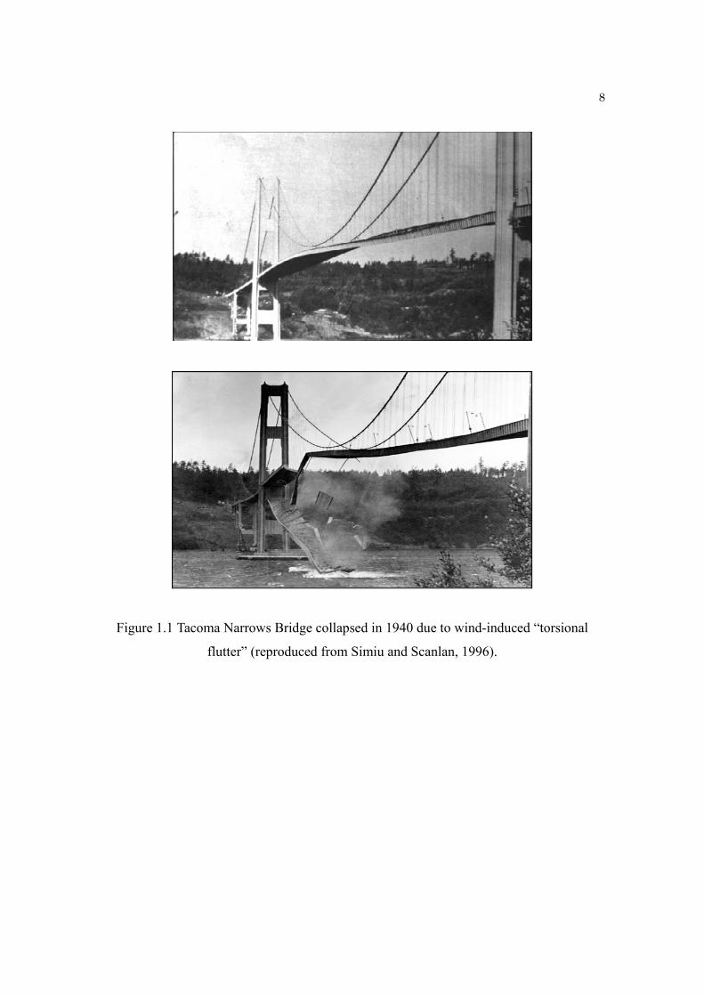
Figure 1.1 Tacoma Narrows Bridge collapsed in 1940 due to wind-induced “torsional flutter” (reproduced from Simiu and Scanlan, 1996). ....................................................... 8
Figure 2.1 A suspension bridge and a section of the deck (Schematic view of a generic finite-element model of the structure). .......................................................................... 29
Figure 3.1 NEU-MIE wind tunnel (Brito 2008). ................................................................. 49
Figure 3.2 Experimental setup: (a) NEU’s small-scale wind tunnel; (b) NEU’s Aeroelastic Force Balance with the truss-type bridge deck model. ....................................... 50
Figure 3.3 The Golden Gate Bridge (Photo courtesy of Google Image). ............................ 51
Figure 3.4 Truss-type deck section model, replicated the features of the Golden Gate Bridge at a scale 1:360; model width is B = 76 mm and the aspect ratio is B/D = 3.5:1. .................................................................................................................... 52
Figure 3.5 Flutter derivatives of a truss-type section model with aspect ratio B/D= 3.5:1 measured at NEU: (a) H1
*; (b) H2*; (c) H3
*; (d) H4*; (e) A1
*; (f) A2*; (g) A3
*; (h) A4
*. ....................................................................................................................... 56
Figure 3.6 Flutter derivatives of a truss-type section model(the Golden Gate Birdge) derived from (Jain et al., 1998): (a) heave Hi
* (i=1,…,4); (b) torsion Ai* (i=1,…,4). ...... 57
Figure 4.1 Flowchart describing the MC-based methodology for buffeting analysis. ......... 87
Figure 4.2 Two-dimensional sample points = 1,000: (a) MC with uniform distribution, (b) QMC with Halton sequence. ............................................................................... 88
Figure 4.3 Ten simplified (sinusoidal-like) mode shapes used in the multi-mode buffeting analysis: (a) LS, 0.049 Hz; (b) VAS, 0.087Hz; (c) LAS, 0.112 Hz; (d) VS, 0.129 Hz; (e) VAS, 0.134 Hz; (f) VS, 0.164 Hz; (g) TAS, 0.192 Hz; (h) TS, 0.197 Hz; (i) VAS, 0.199 Hz; (j) VS, 0.202 Hz. (Note: L is Lateral, V is Vertical, T is Torsional, S is Symmetric, AS is Anti-symmetric). ............................................ 92
Figure 4.4 MC-based scatter plots of RMS response for deck section at x= l/4 and for U = 22.2 m/s as a function of NMC: (a) heave σhh; (b) torsion σαα. ............................. 93
Figure 4.5 Coefficient of variation of the RMS response at x = l/4 for U = 22.2 m/s, computed by MC algorithm: (a) heave σhh; (b) torsion σαα. ................................................. 94

x
Figure 4.6 Tolerance intervals for vertical RMS response (σhh) of 100 MC simulations: (a) NMC = 1,000; (b) NMC = 5,000; (c) NMC = 10,000; (d) NMC = 50,000; (e) NMC = 100,000. ............................................................................................................... 97
Figure 4.7 Tolerance intervals for torsional RMS response (σαα) of 100 MC simulations: (a) NMC = 1,000; (b) NMC = 5,000; (c) NMC = 10,000; (d) NMC = 50,000; (e) NMC = 100,000. ............................................................................................................. 100
Figure 4.8 QMC-based scatter plots of RMS response for deck section at x= l/4 and for U = 22.2 m/s as a function of NQMC: (a) heave σhh; (b) torsion σαα. .......................... 101
Figure 4.9 Coefficient of variation of the RMS response at x = l/4 for U = 22.2 m/s, computed by QMC algorithm: (a) heave σhh; (b) torsion σαα. ............................................ 102
Figure 4.10 Tolerance intervals for vertical RMS response of 100 MC simulations (σhh): (a) NQMC = 1,000; (b) NQMC = 5,000; (a) NQMC = 10,000. ....................................... 104
Figure 4.11 Tolerance intervals for RMS response of 100 MC simulations (σαα): (a) NQMC = 1,000; (b) NQMC = 5,000; (a) NQMC = 10,000. .................................................... 106
Figure 4.12 RMS values for vertical buffeting response as a function of wind speed U corresponding to a given confidence level. ....................................................... 107
Figure 4.13 Flutter derivatives H1* (a) and A2
* (b) of the Golden-Gate Bridge girder with aspect ratio B/D = 3.5:1. Data sets were reproduced from (Jain 1996; Jain et al. 1996) with α0=0°. The (“reference”) coefficients of the “Polynomial Model” were derived by regression of the data sets, according to Eqs. (3.1) and (3.2). Tolerance limits (dashed lines) were based on approximate evaluation of one standard deviation. ........................................................................................................... 108
Figure 4.14 TEP curves of RMS response with respect to thresholds T1 to T3 at the deck section l/4: (a) σhh; (b) σαα (DFV: “Deterministic” Flutter Velocity). ................ 109
Figure 4.15 Procedure for rescaling the TEP curves in Fig. 6.11(c) based on Eq. (6.3): (a) prior probability or TEP; (b) marginal likelihood function; (c) Posterior probability or TEP (DFV: “Deterministic” Flutter Velocity). ........................... 111
Figure 4.16 TEP curves of RMS response at deck section l/4 (T2 threshold only) before (T2) and after rescaling (T2M): (a) σhh; (b) σαα (DFV: “Deterministic” Flutter Velocity). ........................................................................................................................... 112
Figure 4.17 TEP curves of RMS responses with thresholds based on the RMS displacement, deck section at l/4 and NEU’s flutter derivatives: (a) σhh; (b) σαα. .................... 113
Figure 4.18 TEP surfaces of RMS displacement for T2M threshold as a function of wind accounting for effects of skew winds at l/4 with literature flutter derivatives: (a) σhh at l/4; (b) σαα at l/4; (c) σhh at l/2; (d) σαα at l/2. ............................................ 115

xi
Figure 4.19 TEP surfaces of RMS displacement for T2 threshold as a function of wind accounting for effects of skew winds at l/4 with NEU’s flutter derivatives: (a) σhh at l/4; (b) σαα at l/4; (c) σhh at l/2; (d) σαα at l/2. ................................................. 117
Figure 4.20 National Data Buoy Center (NOAA Station 9414290, Latitude: 37.807 N, Longitude: 122.465 W) (Photo reproduced from NOAA, http://www.ndbc.noaa.gov/). ............................................................................. 118
Figure 4.21 PDFs of “parent” (continuous time) mean wind velocity and annual maxima of mean wind velocity, data from NOAA (NOAA). .............................................. 119
Figure 5.1 Reference peak vertical dynamic response, (“deterministic” without variability in FD) as a function of wind velocity at θ = 0° with both Jain’s flutter derivatives and NEU’s flutter derivatives at l/4: (a) displacement; (b) acceleration. .......... 138
Figure 5.2 TEP curves of the peak dynamic response with respect to thresholds T1, T2, T3 deck section at l/4 using Jain’s FD data: (a) vertical response; (b) torsional response. ............................................................................................................ 139
Figure 5.3 Recaled TEP curves (modified by Eq. 4.3) of the peak dynamic response with respect to thresholds T1, T2, T3 deck section at l/4 using Jain’s FD data: (a) vertical response; (b) torsional response. ....................................................................... 140
Figure 5.4 Rescale TEP curves (modified by Eq. 4.3) of the peak dynamic response with respect to thresholds T1, T2, T3 deck section at l/4 using NEU’s FD data: (a) vertical response; (b) torsional esponse. ........................................................... 141
Figure 5.5 A comparison between two sets of curves for vertical response based on NEU’s FD data (continuous lines) and Jain’s FD data (dotted lines): (a) T1=20 milli-g; (b) T2=1m; (c) T3=2m.............................................................................................. 143
Figure 5.6 A comparison between two sets of curves for torsional response based on NEU’s FD data (continuous lines) and Jain’s FD data (dotted lines): (a) T1=20 milli-g; (b) T2=1m; (c) T3=2m.............................................................................................. 145
Figure 5.7 Recaled TEP surfaces (modified by Eq. 4.3) of the peak dynamic vertical response with various intervention levels at l/4 using Jain’s FD data: (a) T1=20 milli-g; (b) T2=1m; (c) T3=2m.............................................................................................. 147
Figure 5.8 Recaled TEP surfaces (modified by Eq. 4.3) of the peak dynamic (normalized to B/2) torsional response with various intervention levels at l/4 using Jain’s FD data: (a) T1=20 milli-g; (b) T2=1m; (c) T3=2m. .......................................................... 149
Figure 5.9 Recaled TEP surfaces (modified by Eq. 4.3) of the peak dynamic vertical response with various intervention levels at l/4 using NEU’s FD data: (a) T1=20 milli-g; (b) T2=1m; (c) T3=2m.............................................................................................. 151
xii
Figure 5.10 Recaled TEP surfaces (modified by Eq. 4.3) of the peak dynamic (normalized to B/2) torsional response with various intervention levels at l/4 using NEU’s FD data: (a) T1=20 milli-g; (b) T2=1m; (c) T3=2m. ................................................. 153
Figure 5.11 Probability distributions of flutter velocity, Ucr, using NEU’s flutter derivatives: a) PDF (probability density function); b) CDF (cumulative density function). 154
Figure 5.12 Resolution of the Monte-Carlo-based flutter procedure vs. standard error. ... 155
Figure 5.13 Intervention costs normalized to the initial construction cost for user comfort level threshold T1=20 milli-g over time based on NEU’s FD data
: (a) 3D PMF (probability mass function stem plot); (b)
2D expected normalized cost, - discount rate/year λ=0.05................................ 156
Figure 5.14 Expected intervention costs normalized to the initial construction cost due to
deformation in deck based on NEU’s FD data : (a) lower
tolerance case (T2=1m); (b) higher tolerance case (T3=2m), - discount rate/year λ=0.05. ............................................................................................................... 157
0 0EC E C t C C
0 0EC E C t C C

xiii
Nomenclature
The following symbols were used in this dissertation:
* *1 4
1 5
damping matrix of the system
,.., flutter derivatives per unit length, torsional moment
,..., constant parameters in Eqs. (5.11a) to (11e)
stiffness matrix of the system
b
A A
b b
B
A
B
0
1
ridge deck width
decay factor
total cost of the structure at time (years)
initial cost of the structure
, random parameters in Eq. (4.1) ( = 1,3,5,7)
cost in present dolli i
j
c
C t t
C
C C j
C
,
ar value
, , drag, lift, moment static coefficients
expected value of maintenance and repair cost
infinitesimal inertia
search direction at step n (FORM)
/ bridge deck, as
D L M
M E
n
C C C
C
dm
B D
d
1
1, 4,
' '1 4
pect ratio
bridge deck height
, random parameters in Eq. (4.2) ( = 1,3,5,7)
,..., "reference" parameters in Eqs. (5.14) (average solution with no errors)
,..., mea
i i
ref ref
D
D D j
D D
D D
1 4
*
n-removed random ,...,
[] expectation operator
system matrix for two-mode aeroeastic instability analyses
complex conjugate transpose of matrix
loss of performance for the bridgv
C C
E
F
Ε
Ε E
,
e
marginal probability density function of
marginal probability density function of
joint probability density function of ,
gust effect factor
g( , ) limit state fu
U
U
cr site
f U
f
f U
g
U U
1, 1 1, 1
nction
,..., modal integrals, simulated bridgest t v vG G

xiv
1
( , ) vertical bridge oscillation, simulated bridges
dimensionless eigen-function of -th mode shape
( ), ( ) modal eigenfunctions, vertical oscillation ( -th mode and mode 1)
/
i
g v
h x t
h i
h x h x g v
h dh
* *1 4
*
0
ˆ peak vertical acceleration
,.., flutter derivatives per unit length, lift force
vertical flutter derivatives ( = 1,...,4)
ˆ imaginary unit
I identity matrix
mass mo
i
dt
h
H H
H i
i
I
g
1 1
ment of inertia per unit length of the deck, simulated bridges
I indicator function
, generalized modal inertias (modes , )
, generalized modal inertia for modes 1 and 1
, re
i j
t v
cr
I I i j
I I t v
K K
1 1
0
duced frequency, reduced critical frequency
, reduced modal frequencies for modes 1 and 1
effective reduced frequency
central span length of the simulated bridges
mass per unit
t v
n
K K t v
K
l
m
length of the bridge deck, simulated bridges
, , aeroelastic drag, lift, moment forces per unit length (Fig. 2.2)
, , bufetting drag, lift, moment forces per unit length (Fig. 2.2)
,
ae ae ae
b b b
D L M
D L M
n
1 1, still-air natural frequency (any, torsional mode 1, vertical mode 1), Hz
number of wind tunnel data points
number of Monte Carlo points
( , ) lateral vibration of the simulat
t v
MC
n n t v
N
N
p x t
ed bridges
dimensionless eigen-function of the -th mode
[] probability function
direction-dependent flutter probabilities
loss of performance of the bridge (threshold )
probab
i
F
T
j
p i
P
P
P T
P
41 1 1 1
ilities of each damage state
flutter probability
flutter probability
-mode shape of the bridge
, dimensionless modal groups (e.g., 0.5 / )
generalized force v
crU
f
i
t v t t
b
j
P
P
q i
q q q B L I
Q ector
generalized force of the -th modeiQ i

xv
standard Gaussian vector
standard error
, , cross PSD of modal loading between two generic sections and
, , auto and cross PSD function of the dynamic response
i j
E
F A B A B
hh h
Q Q
S
S x x K x x
S S S
S
S
modal force cross-spectra
Kaimal spectrum
Lumley-Panofsky spectrum
generic threshold
time
( , ) lateral component of turbulent wind
velocity variable used in conditional
uu
ww
S
S
T
t
u x t
u
*
probability functions (with )
friction velocity
* design point
wind speed, m/s
critical torsional-flutter speed, m/s
normal component of wind speed to the deck, m/s
cr
n
p
u U
u
u
U
U
U
U
,
parallel component of wind speed to the deck, m/s
reduced velocity ( /( ))
reduced critical velocity (at flutter); real root of Eq. (5.12)
wind speed at the bridge site, m/s
(
R
R cr
site
U U nB
U
U
v x
0
, ) horizontal component of turbulent wind
( , ) vertical component of turbulent wind
longitudinal coordinate along the bridge axis
terrain roughness length
( , ) torsional vibrati
t
w x t
x
z
x t
0
1
on of the simulated bridges
dimensionless eigen-function
mean-wind attack angle of the deck
( ), ( ) mode-shape functions, torsional oscillation of the simulated bridges
ˆ unit-gra
i
g t
n
x x
α dient row vector (FORM)
generalized safety index
Kronecker delta function
tolerance parameter (FORM)
dimensionless variance reduction coefficient
ij

xvi
Subscripts and superscripts:
generic mode index for the simulated bridges
generic step of iteration (FORM)
1, 1 fundamental bridge modes, torsional and vertical
† Moore-Penrose pseudo-inverse
g
n
t v
1 1
1 1
1 1
, structural modal damping with respect to critical, modes 1 and 1
generalized coordinate
( ), ( ) generalized modal coordinate, modes 1 and 1
( ), ( ) Fourier transfor
t v
i
t v
t v
t v
t t t v
K K
1 1
,
m of the generalized modal coordinate, modes 1 and 1
two-mode flutter eigenvector = , , with transpose operator
amplitude parameter in FORM
single-mode torsional instabilit
T T
v t
n
t I
t v
ξ
3 4 5 6
1
,
, , 3 4
y equation (see Eq. 5.9)
torsional-mode dimensionless ratio ( / )
value of at critical velocity
air density
, correlation coefficients of random parameters ,
t t
t cr t
D D D D
K K
D D
5 6
' ''
1 1
and ,
standard Gaussian comulative density function
frequency ratio, simple harmonic motion
, maximum positive and minimum negative differences
, , still-air circular fi i
t v
D D
requency (any, torsional and heaving mode), rad/s
critical-flutter circular frequency (torsional mode), rad/s
, , vertical, torsional and lateral RMS displacements
variance of thf
cr
hh pp
P
e flutter-probability MC estimator
still-air circular frequency, rad/s
-th mode natural circular frequency, rad/si i

1
Chapter 1
Introduction
The quantitative analysis of aerodynamic effects on long-span bridges has been considered
(Simiu and Scanlan 1996), since the collapse of the Tacoma Narrows Bridge in 1940 (shown
in Fig. 1.1). Wind engineering researchers have devoted great efforts to understand wind-
induced or “aeroelastic” phenomena (Davenport 1962; Scanlan and Tomko 1971), associated
with the vibration of long-span bridges. “Aeroelastic” is used to indicate fluid-structure
interaction between a flexible structural system and wind air flow. Investigations have also
been performed by many researchers (Kwon 2010; Namini et al. 1992; Scanlan 1987; 1993;
Scanlan and Jones 1990b) to prevent these loading mechanisms from adversely affecting the
satisfactory performance of long-span bridges.
The accurate assessment of fluctuating wind loads on long-span bridges is necessary
to avoid failures or undesired vibrations. Two types of “aeroelastic” phenomena, namely
flutter and buffeting response, are considered in this study. There are the two phenomena
that are relevant for the analysis of bridge deck. Both the potential collapse of the structure
2
due to flutter instability and the dynamic vibration due to wind turbulence (buffeting) at
moderate to high wind speeds are important for bridge design.
Flutter is defined as an oscillatory instability, induced in the bridge deck, when a
bridge is exposed to a wind speed above a certain critical threshold. Beyond this limit,
diverging vibration of the deck is possible, which may result in a catastrophic structural
failure. A classic example of such failures is illustrated in Fig 1.1. Instability can be predicted
through the analysis of flutter derivatives (FDs), and needless to say must be avoided by all
means.
Buffeting is defined as the dynamic vibration regime due to fluctuating loading,
promoted by wind turbulence, which is also influenced by the interaction with structural
deck motion. The bridge vibration is stochastic due to oncoming-flow turbulence and
“signature” turbulence, produced around the deck girder through flow separation and air
recirculation (e.g., (Jones and Scanlan 2001)). The dynamic amplification of vibration,
which causes buffeting, is often observed on long-span bridges (Miyata et al. 2002; Xu et al.
2007; Xu and Zhu 2005). Buffeting does not usually lead to catastrophic failure of the bridge.
However, vibrations cannot be avoided but need to be monitored since they can affect the
serviceability; in fact, damage, fatigue in selected structural elements and user discomfort
are possible.
Both phenomena may occur either separately or together, and can be predicted by
utilizing experimentation in wind tunnel (Bienkiewicz 1987; Ehsan et al. 1993; Huston et al.
1988). Such experimentation is essential for the derivation of wind-induced forces,
especially the loading terms on the deck triggered by fluid-structure interaction; these can
3
be expressed in terms of “flutter derivatives”, originally developed by (Scanlan and Tomko
1971), which are non-dimensional aerodynamic force coefficients per unit deck length as a
function of the “reduced velocity”. Flutter derivatives are the essential parameters in the
estimations of the critical wind velocity of flutter instability and the buffeting response of
long-span cable supported bridges.
Recently, it has been demonstrated that experimentally-derived FDs are random in
nature with uncertainty affected by measurement errors (Sarkar et al. 2009); this uncertainty
in the measurement of the FDs are unavoidable during testing in the wind tunnel. To assess
such uncertainties and the effects on both flutter and buffeting response, it is necessary to
develop specific “analysis tools” which could enable accurate bridge performance
assessment.
This dissertation proposes to develop a methodology for deriving the solution to
buffeting problem on long-span bridges, which will involve the direct representation of the
above-described sources of uncertainty in the aeroelastic input through appropriate statistical
analysis of the FDs.
A second order polynomial model for the FD is proposed and labeled as “model curve”
in this study. The coefficients of this polynomial are treated as random variables, whose
probability distribution is conditional on the reduced wind speed. For computational reasons
in subsequent analysis, however, this dependency is neglected and the probability of these
random variables is treated as independent of the reduced wind speed. For analysis purposes
the first- and second-order statistics are estimated from experiments, treating all the wind
speed data as part of the same population. Wind tunnel experiments are used to validate the
4
proposed methodology and to confirm the relevance of measurement errors in these
aeroelastic force terms. Wind tunnel tests have been conducted at Northeastern University
(NEU) for this purpose.
1.1 Motivation
The prediction and simulation of long-span cable-supported bridge dynamic response due to
wind hazards are particularly difficult in consideration of the inherent complexity of the wind
field, turbulence fluctuations and pressure distributions around the deck (which is the most
vulnerable part of the structure). Experimentation is essential for the derivation of this
dynamic loading. Despite the efforts of the research community towards the development of
refined techniques to simulate full-scale bridge response (Ozkan 2003; Ozkan and Jones
2003), observations can differ from the simulations of the response, based on wind-tunnel
experiments and measurements of equivalent loading. These discrepancies are associated
with the experimental procedures (and their errors) in wind engineering and must be
carefully accounted for in the existing simulation methods.
Reliability analysis against flutter, considering uncertainty in the FDs, has been
investigated by a few researchers (Dragomirescu et al. 2003; Ge et al. 2000; Kwon 2010;
Mannini and Bartoli 2007; Ostenfeld-Rosenthal et al. 1992; Pourzeynali and Datta 2002;
Scanlan 1999). Recently, it has also been shown how to experimentally estimate the
statistical moments of the FDs (variance, co-variance, etc.) from data extracted in wind
tunnel tests (Kwon 2010; Mannini et al. 2012).

5
However, very limited emphasis has been given to structural serviceability due to
uncertainty in buffeting loading (Caracoglia 2008a). With the aging bridge inventory in the
United States, it is therefore important to advance the current analysis approaches to include
the “statistical buffeting” response. The term “statistical buffeting” analysis is coined for the
first time in this dissertation to differentiate from the standard buffeting analysis in the
absence of uncertainty in the FD.
This dissertation focuses on the development of a methodology for “statistical
buffeting” analysis, including the uncertainty in the FD. To accomplish these tasks and, most
importantly, a second order polynomial model (“model curve”) for the FD is proposed. The
model curve is a second order polynomial description of the FDs where uncertainty is
associated with coefficient of the polynomial. This curve is used to describe the behavior of
the flutter derivatives as a function of reduced velocity. The physical justification for this
selection stems from the observation that the FDs tend to follow a general trend, especially
for moderately bluff deck sections (Simiu and Scanlan 1996). Therefore, postulating such a
“model curve” for FDs was selected as an appropriate assumption for projecting the
variability of the coefficients of the model curve into the analysis of the buffeting response
of the bridge.
In the standard approach the result of the buffeting analysis is the value of the RMS
dynamic response at a given wind speed. In the proposed probabilistic setting one estimates
the probability that a given threshold for the variance of the response is exceeded. This
probability is later used, together with information on the probability of the wind velocity at
a given site, to predict “lifetime expected cost” (Wen and Kang 2001) due to the buffeting

6
response of a 1200-meter suspension bridge (a function proportional to the cost associated
with interventions needed to ensure safety or for maintenance) is affected by the variability
of the FDs.
Even though the ultimate goal of the research is the development of a generalized
methodology for the solution to buffeting problems on long-span bridges for the analysis of
the effects induced by various sources of uncertainty; this should involve the extension of
the procedures and should include both wind-loading input and selected structural properties.
This dissertation represents a first step towards this objective.
1.2 Outline
This dissertation is divided into the following chapters, after providing a general introduction
and motivation in Chapter 1.
Chapter 2 summarizes the background theory of wind-induced response of long-span
bridges and reviews the fundamental aspects of aerodynamics and aeroelasticity of long-
span suspended bridge decks.
Chapter 3 describes the development of a “model curve” for representation of the
behavior of flutter derivatives as a function of reduced wind velocity. This chapter also
describes the experimental setup, measurements and experimental results, used in this
research. Flutter derivatives were measured in the wind tunnel at NEU.
Chapter 4 describes the standard buffeting analysis of long-span bridges
(“deterministic case”) as well as “statistical buffeting” analysis which includes the variability
in the FD. The “statistical buffeting” response was evaluated by adopting the concept of

7
“fragility”; this was employed in the calculation of the exceedance probability of pre-
selected vibration thresholds, conditional on mean wind speed and direction at the deck level.
Chapter 5 discusses the lifetime estimation of monetary losses for a long-span bridge,
designated as “cost analysis”, due to buffeting response. The expected value of the loss
function (lifetime cost estimation) of a 1200-meter suspension bridge is evaluated by
applying the “statistical buffeting” analysis. Summary of the work, conclusions of the
dissertation and directions for future research are discussed in Chapter 6.
8
Figure 1.1 Tacoma Narrows Bridge collapsed in 1940 due to wind-induced “torsional
flutter” (reproduced from Simiu and Scanlan, 1996).

9
Chapter 2
Wind-Induced Response of Long-Span Bridges: Review
This chapter reviews the fundamental aspects of aerodynamics and aeroelasticity of long-
span suspended bridge decks. Figures 2.1 and 2.2 show a section view of the bridge deck to
be analyzed. The wind-induced dynamic response of a long-span bridge close to aeroelastic
instability is most conveniently analyzed in the frequency domain, as described by (Jain
1996; Jones and Scanlan 2001; Katsuchi et al. 1999); this method, referred to as “multi-
mode” approach in wind engineering, is reviewed in this chapter.
2.1 General Formulation
The deflection components of the bridge deck (i.e., h(x,t), p(x,t) and α(x,t) in Fig. 2.2) can
be expressed in terms of the generalized coordinate of the mode ξi(t), the deck width B and
the dimensionless representations of the i-th mode form along the deck hi(x), pi(x) and αi(x)
as
10
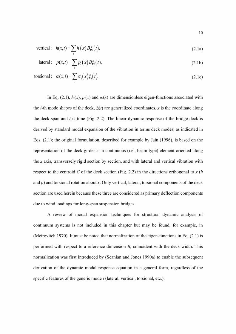
vertical : ( , ) ,i ii
h x t h x B t (2.1a)
(2.1b)
torsional : (x,t)
ix i
t i . (2.1c)
In Eq. (2.1), hi(x), pi(x) and αi(x) are dimensionless eigen-functions associated with
the i-th mode shapes of the deck, ξi(t) are generalized coordinates. x is the coordinate along
the deck span and t is time (Fig. 2.2). The linear dynamic response of the bridge deck is
derived by standard modal expansion of the vibration in terms deck modes, as indicated in
Eqs. (2.1); the original formulation, described for example by Jain (1996), is based on the
representation of the deck girder as a continuous (i.e., beam-type) element oriented along
the x axis, transversely rigid section by section, and with lateral and vertical vibration with
respect to the centroid C of the deck section (Fig. 2.2) in the directions orthogonal to x (h
and p) and torsional rotation about x. Only vertical, lateral, torsional components of the deck
section are used herein because these three are considered as primary deflection components
due to wind loadings for long-span suspension bridges.
A review of modal expansion techniques for structural dynamic analysis of
continuum systems is not included in this chapter but may be found, for example, in
(Meirovitch 1970). It must be noted that normalization of the eigen-functions in Eq. (2.1) is
performed with respect to a reference dimension B, coincident with the deck width. This
normalization was first introduced by (Scanlan and Jones 1990a) to enable the subsequent
derivation of the dynamic modal response equation in a general form, regardless of the
specific features of the generic mode i (lateral, vertical, torsional, etc.).
lateral : ( , ) ,i ii
p x t p x B t

11
The governing generalized equation of motion of mode i (ξi) therefore becomes (e.g.,
Scanlan and Jones, 1990)
I
i
i 2
i
i
i
i2
i Q
it , (2.2)
where Ii and Qi(t) are the generalized inertia and modal force of the i-th mode, ωi and ζi are
the i-th mode natural circular frequency and the modal damping ratio.
The generalized inertia Ii is defined as
2 , , , , ,i istructureI q x y z dm x y z (2.3a)
where qi (x, y, z) are the i-th mode shape of the bridge and dm is an infinitesimal inertia; this
equation is written in a general form to emphasize that the integration may be carried out
over the entire structure to also account for modal mass contributions from portions of the
bridge other than the deck itself, which are also involved in the vibration; these terms depend,
for example, on the moving cables in a suspension bridge or the tower motion. If the mass
and moment of inertia of the moving deck and cables are assumed as constant along x, and
respectively expressed by m0 and I0 per unit deck length, the modal inertia, using the
expansion in Eq. (2.3a), simply becomes
2 2 2 2 20 0 00
,l
i i i iI m h x B m p x B I x dx (2.3b)

12
in which l is the total deck length.
The generalized force Qi(t) due to wind loading is given in a similar form by Eq.
(2.4).
0
, , , ,l
i i i iQ t L x t h x B D x t p x B M x t x dx (2.4)
where L(x,t), D(x,t) and M(x,t) represent the lift, drag and pitching moment per unit span
length (in Fig. 2.2). They are assumed to be separable into motion-dependent loads and
turbulence-induced loads (motion-independent) and are defined as
lift : ae bL L L (2.5a)
drag: ae bD D D (2.5b)
moment : ae bM M M (2.5c)
where the subscripts ae and b refer to aeroelastic and buffeting loads, respectively. The
aeroelastic (or self-excited forces) are assumed to be linearizable. For purely sinusoidal
motions of frequency ω, the aeroelastic forces can be expressed as (Scanlan and Tomko
1971).
Lae
1
2U 2B KH
1*h
U KH
2* B
U K 2H
3* K 2H
4* h
B KH
5* p
U K 2 H
6* p
B
, (2.6a)

13
Dae
1
2U 2B KP
1* p
U KP
2* B
U K 2P
3* K 2P
4* p
B KP
5*h
U K 2P
6* h
B
, (2.6b)
Mae
1
2U 2B2 KA
1*h
U KA
2* B
U K 2 A
3* K 2 A
4* h
B KA
5* p
U K 2 A
6* p
B
, (2.6c)
where is the air density, U the mean velocity of the oncoming wind (which is turbulent
in general) at the deck level, K (= ωB/U) is the reduced frequency with ω circular frequency;
/h dh dt , d / dt and /p dp dt pertain to the deck section at x. In Eq. (2.6), Hi* Pi
*
and Ai* (with i = 1,…,6) are flutter derivatives of the deck cross-section. As noted by Scanlan
and Tomko (1971), the previous expressions are written in a mixed time-frequency form and
are valid for simple harmonic motion of the deck at a given ω; this assumption is strictly
valid at flutter but is acceptable in the case of vibration induced by turbulence disturbances
on low-damping systems, such a suspension bridge. Equations were derived by extension of
the standard airfoil theory (Theodorsen 1935) to non-aerodynamic (bluff) bridge deck
sections. It must be noted that the frequency-time duality is only apparent since it disappears
once Fourier-domain analysis is employed to derive the bridge response (Scanlan and Tomko
1971), as later described.
Buffeting forces per unit length are fluctuating loads which can be described by
“quasi-steady theory” and turbulence disturbances for vibration about a static equilibrium
configuration of the deck due to mean wind loads. For mean incident wind orthogonal to the
bridge axis, the loading depends on the vertical (w), and lateral (u) turbulence, which are
stochastic quantities as a function of time t and position x along the deck (Fig. 2.2). For small
vibration amplitudes these can be obtained by first-order expansion about on equilibrium
14
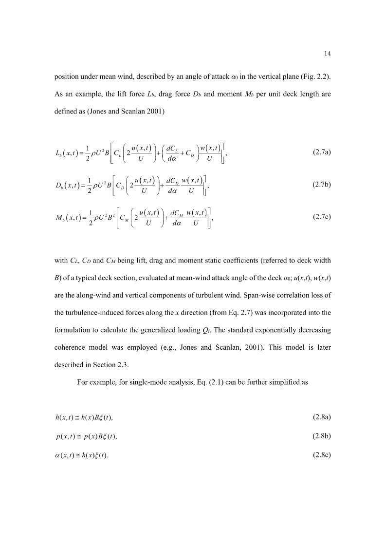
position under mean wind, described by an angle of attack α0 in the vertical plane (Fig. 2.2).
As an example, the lift force Lb, drag force Db and moment Mb per unit deck length are
defined as (Jones and Scanlan 2001)
2 , ,1, 2 ,
2L
b L D
u x t w x tdCL x t U B C C
U d U
(2.7a)
2 , ,1, 2 ,
2D
b D
u x t w x tdCD x t U B C
U d U
(2.7b)
2 2 , ,1, 2 ,
2M
b M
u x t w x tdCM x t U B C
U d U
(2.7c)
with CL, CD and CM being lift, drag and moment static coefficients (referred to deck width
B) of a typical deck section, evaluated at mean-wind attack angle of the deck α0; u(x,t), w(x,t)
are the along-wind and vertical components of turbulent wind. Span-wise correlation loss of
the turbulence-induced forces along the x direction (from Eq. 2.7) was incorporated into the
formulation to calculate the generalized loading Qi. The standard exponentially decreasing
coherence model was employed (e.g., Jones and Scanlan, 2001). This model is later
described in Section 2.3.
For example, for single-mode analysis, Eq. (2.1) can be further simplified as
( , ) ( ) ( ),h x t h x B t (2.8a)
( , ) ( ) ( ),p x t p x B t (2.8b)
( , ) ( ) ( ).x t h x t (2.8c)
15
Similarly, the dynamic loading Qi in Eq. (2.4) becomes a scalar term. The multi-mode
system of equations can be formed by separating the generalized loading Qi(t) into
aeroelastic and buffeting components Qi(t)=Qae,i(t)+Qb,i(t) and by recognizing that the
loading induced by Qae,i(t) is linearly dependent quantities related to dynamic motion and
velocity of the deck sections; therefore, Qae,i(t) can be expressed as a linear function of the
generalized displacements and velocities through Eq. (2.1) and the effect of Qae,i(t) on the
bridge can be interpreted as a modification to the generalized stiffness and damping of the
structural modes which depend on wind speed U. A more detailed description may be found
in Scanlan and Jones (1990). The generic scalar Eq. (2.2) can be simplified as
i 2
i
i
i
i2
i Q
ae,it I
i Q
b,it I
i and the left-hand side rewritten by regrouping
terms as a function of Qae,i(t)/Ii as wind-induced stiffness and damping equivalent quantities.
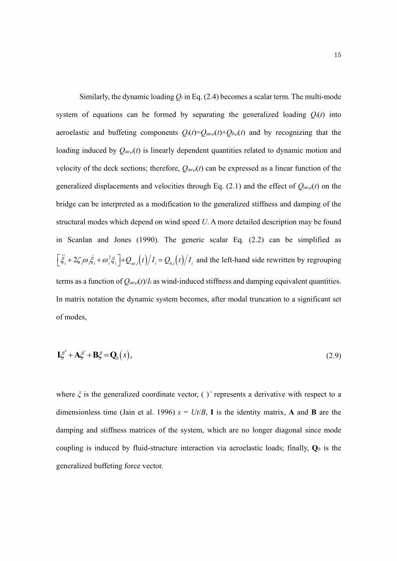
In matrix notation the dynamic system becomes, after modal truncation to a significant set
of modes,
'' ' ,b s I A B Q (2.9)
where ξ is the generalized coordinate vector, ( )’ represents a derivative with respect to a
dimensionless time (Jain et al. 1996) s = Ut/B, I is the identity matrix, A and B are the
damping and stiffness matrices of the system, which are no longer diagonal since mode
coupling is induced by fluid-structure interaction via aeroelastic loads; finally, Qb is the
generalized buffeting force vector.
16
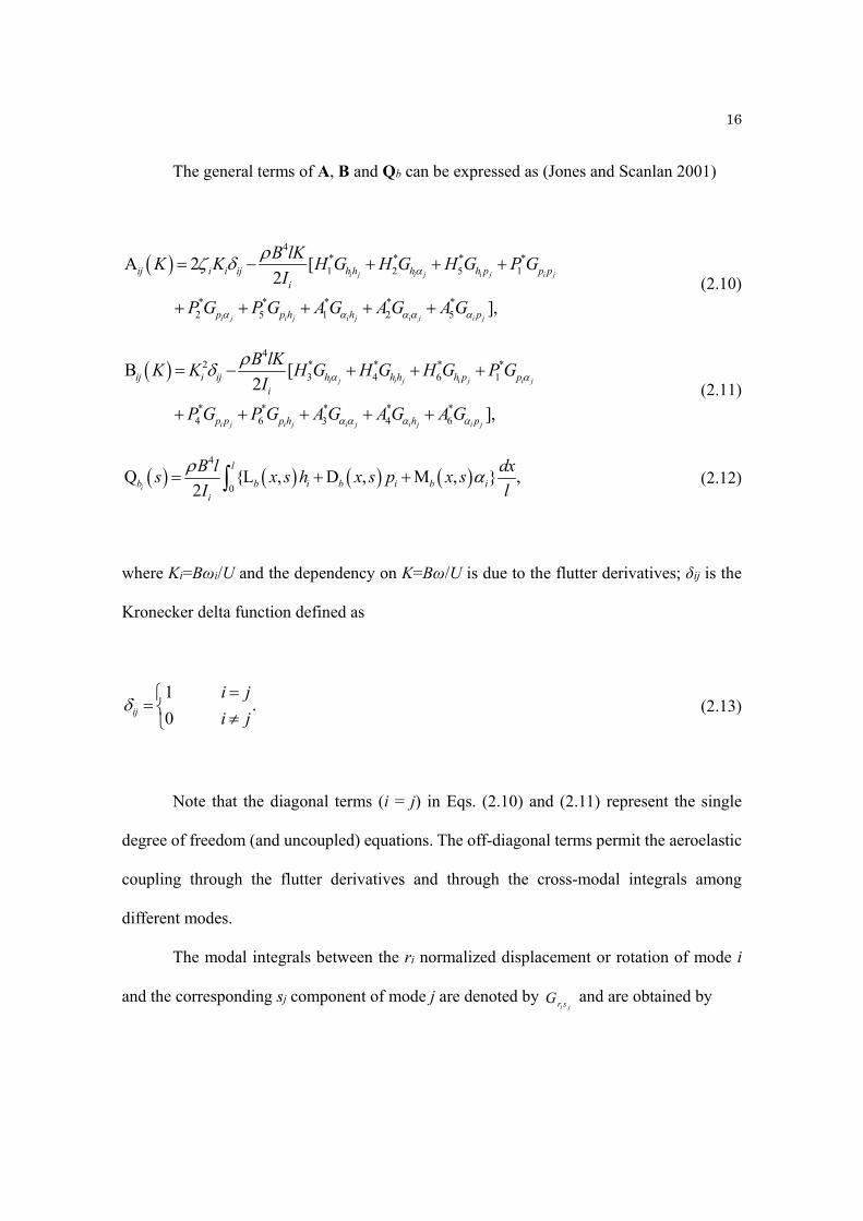
The general terms of A, B and Qb can be expressed as (Jones and Scanlan 2001)
4
* * * *1 2 5 1
* * * * *2 5 1 2 5
A 2 [2
],
i j i j i j i j
i j i j i j i j i j
ij i i ij h h h h p p pi
p p h h p
B lKK K H G H G H G P G
I
P G P G A G A G A G
(2.10)
4
2 * * * *3 4 6 1
* * * * *4 6 3 4 6
B [2
],
i j i j i j i j
i j i j i j i j i j
ij i ij h h h h p pi
p p p h h p
B lKK K H G H G H G P G
I
P G P G A G A G A G
(2.11)
4
0Q {L , D , M , } ,
2i
l
b b i b i b ii
B l dxs x s h x s p x s
I l
(2.12)
where Ki=Bωi/U and the dependency on K=Bω/U is due to the flutter derivatives; δij is the
Kronecker delta function defined as
1.
0ij
i j
i j
(2.13)
Note that the diagonal terms (i = j) in Eqs. (2.10) and (2.11) represent the single
degree of freedom (and uncoupled) equations. The off-diagonal terms permit the aeroelastic
coupling through the flutter derivatives and through the cross-modal integrals among
different modes.
The modal integrals between the ri normalized displacement or rotation of mode i
and the corresponding sj component of mode j are denoted by i jr sG and are obtained by

17
0( ) ( ) ,
i j
l
r s i j
dxG r x s x
l (2.14)
where ri = hi, pi or αi, sj = hj, pj or αj.
The new system of equations can be Fourier transformed into the reduced frequency
(K) domain (Scanlan and Jones 1990a); for example a generic time-dependent function f(s)
with s = Ut/B becomes in the frequency domain with ˆ 1i :
ˆ
0.iKsf K f s e ds
(2.15)
Consequently, a system of equations, exclusively dependent on K and, is derived
from Eq. (2.9) as
,b E Q (2.16)
where and bQ are the Fourier-transformed ˆ
0
iKsK s e ds and bQ vectors,
respectively. A general term of the “impedance matrix” E is
2 ˆ .ij ij ij ijE K iKA K B K (2.17)

18
2.2 Background on Flutter
A review of flutter theory is presented in this section. Information was derived from (Jain
1996; Katsuchi 1997). Flutter is an oscillatory instability induced when a bridge is exposed
to a wind speed above a certain critical threshold. Beyond this limit, diverging vibration of
the deck is possible, which may result in a catastrophic structural failure. One particular
example was the Tacoma Narrows incident in 1940 when such phenomenon was clearly
recognized. Flutter instability must be avoided by all means in bridge engineering.
Aeroelastic instability can be predicted by analyzing the aeroelastic coefficients of bridge
decks (flutter derivatives in Eq. 2.6) developed by (Scanlan and Tomko 1971), which are
employed for simulating the dynamic response of the bridge. Flutter derivatives in Eq. (2.6)
are force coefficients per unit length, routinely measured in wind tunnel tests. As briefly
outlined in a previous section, these expressions of the shape-dependent force coefficients
of the moving deck section have been strongly influenced by airfoil theory for streamlined
bodies (Theodorsen 1935), from which they have been derived for use in civil engineering
applications.
Frequency-domain analysis was used in this study; this is the preferred method of
bridge dynamic researchers because this analysis can be related to direct physical
interpretation through flutter derivatives, obtained experimentally, as opposed to time-
domain analysis, which requires modeling of the Qae,i(t) loading in terms of convolution
integrals (Scanlan et al. 1974) and a more complex formulation (on occasion suffering from
the lack of physical interpretation; (Caracoglia and Jones 2003).

19
The flutter condition is identified by solving the aeroelastically influenced effective
damping problem derived from Eq. (2.16) by setting the turbulence-induced loading 0bQ
(Jones and Scanlan 2001; Katsuchi et al. 1998).
. E 0 (2.18)
Equation (2.18) can be reduced to the nontrivial solution of the complex algebraic
system. However, a direct method for the solution of det[E] is not available because the
matrix E includes two unknown variables, K and ω. The matrix E also consists of complex
numbers so that the condition of det[E]=0 must be satisfied with both the real and imaginary
parts of the determinant simultaneously equal to zero. An iterative procedure is needed to
solve for det[E]=0 (Jones and Scanlan 2001). This can be accomplished by fixing a value of
K and seeking a value of ω, in the frequency range of interest, for which the determinant is
zero, and changing the value of K until both the real and imaginary determinants are zeros
at the same ω. Once the values K (= ωB/U) and ω are obtained with satisfying Eq. (2.18),
the flutter speed can be calculated.
For a multi-mode problem, the same procedure is required and the largest value of K
of all solutions gives the flutter-critical condition. The mode corresponding to the solution
of ω is the leading mode in the flutter condition. Moreover, the eigenvector ξ at the flutter
condition gives the flutter mode shape which indicates the relative participation of each
structural mode in flutter vibration.

20
2.3 Background on Buffeting
A review of buffeting theory is presented in this section; the material has been derived from
(Jain 1996; Katsuchi 1997). Buffeting is a dynamic phenomenon, in which the wind-induced
loading is dynamic and due to wind turbulence. The bridge vibration is stochastic due to
oncoming-flow turbulence or signature turbulence, enhanced by flow separation and
recirculation around the deck girder (e.g., (Jones and Scanlan 2001)).
The vector of buffeting forces on the right hand side of Eq. (2.16) is
1
2
01
40
2
0
1F
1F
,2
1F
n
l
b
l
b
b
l
bn
dx
I l
dxB l
I l
dx
I l
Q
(2.19)
where the integrands in the vector above are the Fourier transforms of the Eq. (2.12).
F , L , D , M , .ib b i b i b ix K x K h x x K p x x K x (2.20)
By substituting the terms L b, Db
and Mbfrom Eqs. (2.7a – 2.7c) at the span location
xA, Eq. (2.20) leads to
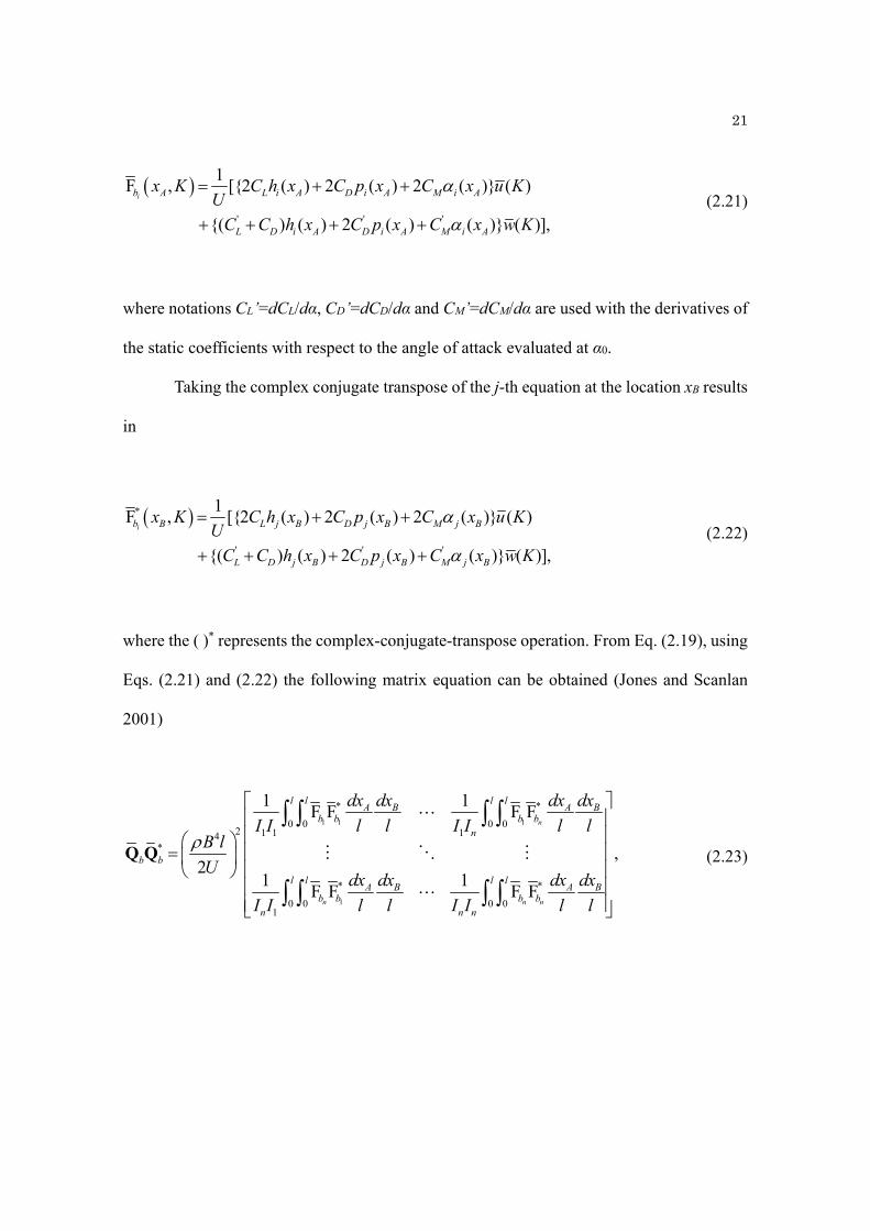
21
' ' '
1F , [{2 ( ) 2 ( ) 2 ( )} ( )
{( ) ( ) 2 ( ) ( )} ( )],
ib A L i A D i A M i A
L D i A D i A M i A
x K C h x C p x C x u KU
C C h x C p x C x w K
(2.21)
where notations CL’=dCL/dα, CD’=dCD/dα and CM’=dCM/dα are used with the derivatives of
the static coefficients with respect to the angle of attack evaluated at α0.
Taking the complex conjugate transpose of the j-th equation at the location xB results
in
*
' ' '
1F , [{2 ( ) 2 ( ) 2 ( )} ( )
{( ) ( ) 2 ( ) ( )} ( )],
ib B L j B D j B M j B
L D j B D j B M j B
x K C h x C p x C x u KU
C C h x C p x C x w K
(2.22)
where the ( )* represents the complex-conjugate-transpose operation. From Eq. (2.19), using
Eqs. (2.21) and (2.22) the following matrix equation can be obtained (Jones and Scanlan
2001)
1 1 1
1
* *
0 0 0 02 1 1 14
*
* *
0 0 0 01
1 1F F F F
,2
1 1F F F F
n
n n n
l l l lA B A B
b b b bn
b b
l l l lA B A B
b b b bn n n
dx dx dx dx
I I l l I I l lB l
Udx dx dx dx
I I l l I I l l
Q Q
(2.23)
22
from which the turbulence-induced dynamic response of the bridge can be derived by
standard random vibration techniques (e.g., (Newland 1993). The power spectral density
(PSD) matrix of the generalized loading can be calculated, a general term of which is
24
0 0
1, ,
2
, , ,
b bi j
l l
Q Q i A j B uu A Bi j
A Bi A j B ww A B
B lS K q x q x S x x K
U I I
dx dxr x r x S x x K
l l
(2.24)
where
2 ,i L i D i M iq x C h x C p x C x (2.25)
' ' '2 .i L D i D j M jr x C C h x C p x C x (2.26)
The equations above depend on the cross-power spectral densities of the lateral
turbulence Suu(xA,xB,K) and vertical turbulence Sww(xA,xB,K). The uw-cross spectrum of the
wind Suw has not been included in the equation above as it is usually of secondary importance
on the dynamic response. A more complete formulation may be found in (Jain 1996).
If the auto-power spectral density of the wind components is independent of the
location x along the deck axis, the span-wise cross-spectral densities of the wind components
in conventional form as (Scanlan and Tomko 1971)
23
, , exp ,2A B A B
cKF x x K F K x x
B
(2.27)
where c is a decay factor, the range of which is generally taken as
8 16nl nlc
U U . (2.28a)
Therefore, the cross-power spectral densities Suu(xA,xB,K) and Sww(xA,xB,K) can be
simplified as
( , , ) exp ,2
( , , ) exp .2
uu A B A Buu
ww A B A Bww
cKS x x K S K x x
B
cKS x x K S K x x
B
(2.28b)
The limits in Eq. (2.28b) can be used for force calculations to reflect the higher span-
wise correlation in the pressure loading than the one seen in the velocity components (Larose
1992). Using the following expressions
0 0
exp ,2i j
l lA B
rs i A j B A B
dx dxcKH K r x s x x x
B l l (2.29)
where ri and si = hi, pi or αi, the ij-th term of the buffeting force matrix can be expressed as

24
24 1
,2b bi j
Suu SwwQ Q ij uu ij ww
i j
B lS K Y K S K Y K S K
U I I
(2.30)
where
2 2 22 2 2
4 4
4 ,
i j i j i j
i j i j i j i j
i j i j
Suuij L h h D p p M
L D h p p h L M h h
D M p
Suuij
Suuij p
Y K C H C H C H
C C H H C C H H
C C H
K
K H
Y
Y
(2.31)
2 2 2' ' '
' ' ' '
' ' .
i j i j i j
i j i j i j i j
i j i j
Swwij L D h h D p p M
L D D h p p h L D M h h
D M p p
Y K C C H C H C H
C C C H H C C C H H
C C H H
(2.32)
The power spectral of the wind components u and w in the atmospheric boundary
layer, expressed as functions of K, are assumed as (Simiu and Scanlan 1996)
2*
5/3
200,
1 502
uu
zuS K
KzU
B
(2.33)
2*
5/3
3.36.
1 102
ww
zuS K
KzU
B
(2.34)
25
The first equation above is the “Kaimal spectrum”; the second expansion is the
“Lumley-Panofsky spectrum”. In the previous equations z is the elevation above ground and
u* is the friction velocity, a function of the surface roughness. The friction velocity u* can be
determined by using
*
1ln ,
o
zU z u
k z (2.35)
where U(z) is the mean wind velocity at elevation z (usually taken as the velocity at the deck
level, U), k is the von Kármán constant which is generally assumed to be 0.4k (Simiu and
Scanlan 1996) and z0 is the terrain roughness length.
The power spectral density matrix for the generalized displacements ξ is developed
in dimensionless form using Eq. (2.16) as
11 *( ) ( ) ( ) ,b bQ QK K K K
S E S E (2.36)
where E* is the complex conjugate transpose of matrix E.
The PSD of the physical displacements (Eqs. 2.1a – 2.1c) can be obtained from the
PSD of the respective generalized displacement components through
2, , ,i jhh A B i A j B
i j
S x x K B h x h x S K (2.37)
26
2, , ,i jpp A B i A j B
i j
S x x K B p x p x S K (2.38)
, , ,i jA B i A j B
i j
S x x K x x S K (2.39)
where i and j are summed as the summation over the number of modes being used. Cross-
spectral densities can be developed in a similar manner.
Evaluation of the spectral densities of the displacements at combinations of discrete
xA and xB will result in a matrix. The mean-square values of these displacements can be
evaluated in terms of their respective PSD functions.
2
0
2,hh hh
BS K dK
U
(2.40a)
2
0
2,pp pp
BS K dK
U
(2.40b)
2
0
2,
BS K dK
U
(2.40c)
where K is the reduced frequency.
A covariance matrix for h, p and α is thus obtained, from which statistics of the
displacement components h, p and α can be calculated. A use of the reduced frequency, K,
as the variable of integration results in an additional factor of 2πB/U in the estimation of
mean-square value.
27
2.4 Effect of Wind Directionality: Skew Wind Theory
In the previous sections, considering the wind as it approaches the bridge orthogonal to the
deck axis derives basic flutter and buffeting studies. However, in nature, the highest winds
of record at a given site is very likely to be skew to the bridge (Scanlan 1999). Therefore,
flutter and buffeting analyses are modified to account for directionality θ (mean-wind yaw
angle in Fig. 2.3), as originally proposed in (Scanlan 1993).
A review of skew wind buffeting theory is presented in this section. The material is
derived from (Scanlan 1993). In Fig. 2.3, the plan view of the deck is shown with steady
mean wind velocity U and accompanying turbulence components (i.e., u(t), v(t) and w(t))
and approaching the bridge at an angle θ with respect to the direction orthogonal to the deck
axis indicated by the normal y (or y(n) in Fig. 2.3). As explained in (Scanlan 1993), the effect
of a skew wind on the bridge vibration can be estimated by considering a component Un
normal (across-deck) to the deck of mean wind velocity and two turbulence components u
and v as
co s sin ,nU U u v (2.41)
s in co s .pU U u v (2.42)
The effect of the parallel (along-deck) component to the deck Up, usually of minimal
relevance, was neglected in this research. As an example, vertical and torsional aeroelastic
loadings due to two components of skew wind U shown in Fig. 2.3 can be constructed by
replacing the original expressions by means of a reduced skew frequency Kn:
28
Lae
1
2U 2 B K
nH
1*h
U K
nH
2* B
U K
n2H
3* K
n2H
4* h
B
, (2.43)
Mae 1
2U 2B2 Kn A1
*h
U Kn A2
* B U
Kn2 A3
* Kn2 A4
* h
B
, (2.44)
where given the reduced K = Bω/U, the normal component becomes Kn = K/cosθ. Flutter
derivatives in previous equations are also evaluated at Kn (sometimes referred to as the
“cosine rule”).
Similarly, buffeting loads can be constructed due to skew wind effect as follows:
21cos 2 2 sin ,
2L
b L D L
v tdCu wL U B C C C
U d U U
(2.45)
2 21cos 2 2 sin ,
2M
b M M
v tdCu wM U B C C
U d U U
(2.46)
with static coefficients evaluated at α0, CD, CL and CM.
This formulation can be recast in Eqs. (2.37 – 2.40) as a function of u, v, w, θ and Kn
and can be used directly into the framework of the multimode algorithm, introduced in the
previous sections.

29
Figure 2.1 A suspension bridge and a section of the deck (Schematic view of a generic
finite-element model of the structure).
Figure 2.2 Degrees of freedom and aeroelastic forces on a bridge deck (the p component neglected in this study).

30
Figure 2.3 Schematic plan view of bridge deck with skew wind approaching the girder at wind speed U with turbulence components u, v, w and skew wind angle θ (Scanlan 1993).
θ U+u(t)
v(t)
w(t)
Up
Un
BBridge Deck
y (n)
x

31
Chapter 3
A Second-order Polynomial Model for Flutter
Derivatives
This chapter introduces the concept of “model curve”, a polynomial-based function for
flutter derivatives in terms of reduced velocity and used to describe in a generalized form;
the coefficients of this polynomial are random variables considering the uncertainty in the
flutter derivative (FD). Probability distribution or the random variables is conditional on the
reduced wind speed. For computational reasons in subsequent analysis, however, this
dependency is neglected and the probability of these random variables is treated as
independent of the reduced wind speed. For analysis purposes the first- and second-order
statistics are estimated from experiments, treating all the wind speed data as part of the same
population. Experiments were conducted in the wind tunnel, maintained by the Department
of Mechanical and Industrial Engineering at Northeastern University (NEU).
This chapter describes the experimental methods and wind tunnel tests, employed for
the extraction of aeroelastic coefficient or flutter derivatives (FDs) and also for the
32
estimation of the first- and second-order statistics of the polynomial model. Section models,
representing a section of the deck in a long-span bridge, were used in the study. These models
are intended to represent only a portion of the deck of the bridge, i.e., the section
schematically shown in Fig. 2.2. The description of the wind tunnel and bridge models used
in this study are given. The FDs were found simultaneously from two-degree-of-freedom
(two-DOF) coupled motion section model tests.
The model curve will be later used in Chapters 4 and 5, which enables to directly
project the uncertainty in the FD into the analysis of the buffeting response of the bridge
3.1 Description of the Polynomial Model and Discussion on its Physical
Interpretation
3.1.1 Description of the Polynomial Model
It has been shown (e.g., Scanlan and Tomko, 1971) that most flutter-derivative experimental
curves tend to follow a similar trend, especially for relatively bluff deck sections (Simiu and
Scanlan 1996). Postulating a second order polynomial model for flutter derivatives (FDs) to
describe the evolution of flutter derivatives as a function of reduced velocity was proposed
as a physically acceptable assumption in the context of simulation. The polynomial, labeled
as “model curves”, for FDs as a function of reduced velocity UR=2π/K with i = 1,...,4 are
shown below:
* 21 ,i R j R j RH U C U C U
1,..., 4 1,3,5,7i j (3.1)
* 21 .i R j R j RA U D U D U
1,..., 4 1,3,5,7i j (3.2)
33
These parameters become Cj and Cj+1 for Hi*, Dj and Dj+1 for Ai
*. The general form
for all Hi* and Ai
* derivatives can be expressed as in Eqs. (3.1–3.2) with i=1,…,4 and
j=1,3,5,7. In Eq. (3.1), Cj and Cj+1 are constant parameters of the model, which are assumed
as random coefficients and can be related in a simple way to experimental errors. The mean
values of Cj and Dj can be determined from the mean of experimental points, extracted at
various wind speeds in wind tunnel; similarly, second-moment properties of Cj and Dj can
be related to the variances of measured FDs; the coefficients of the polynomial are
determined from statistical regression of the experimental data, described in a separate sub-
section.
3.1.2 Discussion on the Selection of the Polynomial Model, based on Physical
Behavior of Flutter Derivatives
It must be noted that the selection of the model curves, based on a second order polynomial,
is not arbitrary but has a direct interpretation with the physical phenomenon related to the
concept of FD. FDs are employed to describe the unsteady fluid-structure interaction.
Nevertheless, as a first approximation, the Hi* and Ai
* coefficients can be estimated by using
a suitable combination of the static lift and moment coefficients of the deck section model,
measured in a “static test” of the model, rigidly mounted on a fixed force balance (e.g., Simiu
and Scanlan, 1996). Using the general theory of quasi-stationary wind forces (e.g., Simiu
and Scanlan, 1996) and recalling that “air inertial” contributions are negligible in this
formulation (whence H*4, A*
4 derivatives cannot be evaluated), the approximate expressions
34
of the flutter derivatives as a function of reduced frequency K=2π/UR for initial angle of
attack α0 close to zero are (Singh 1997; Strømmen 2006)
0 0 00 0 0* * *1 2 3 2
, , ,
L L LdC dC dCd d d
H H HK K K
(3.3a)
0 0 00 0 0* * *1 2 3 2
, , .
M D MdC dC dC
d d dA A A
K K K
(3.3b)
In the expressions above the derivation with respect to the static angle of attack α is
applied to the static lift coefficient (CL) and moment coefficient (CM), which are constant
and independent of flow speed. Expressions above are inversely proportional to K (with
exponent at most equal to 2) or, in other words, proportional to the reduced velocity UR with
the same exponent. The equations above show that flutter derivatives can be theoretically
interpreted as a “monomial” in terms of reduced velocity (inverse of K), which is at most of
order two. Since the expressions above are theoretically valid for low K only (K of the order
0.2 to 0.4) only (Strømmen 2006) it is reasonable to assume a polynomial expression as the
most plausible model for the derivatives, based on physical evidence. Therefore, the use of
Eqs. (3.1) and (3.2) in the model curves is justified by physical evidence. This interpretation
is, however, valid for linear superposition of aeroelastic effects, because of the use of the
static coefficients in Eq. (3.3) and for small vibrations h or α compared to the reference
dimension of the deck (width B or depth D).
35
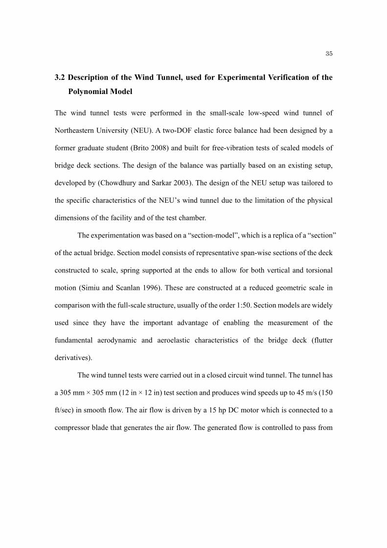
3.2 Description of the Wind Tunnel, used for Experimental Verification of the
Polynomial Model
The wind tunnel tests were performed in the small-scale low-speed wind tunnel of
Northeastern University (NEU). A two-DOF elastic force balance had been designed by a
former graduate student (Brito 2008) and built for free-vibration tests of scaled models of
bridge deck sections. The design of the balance was partially based on an existing setup,
developed by (Chowdhury and Sarkar 2003). The design of the NEU setup was tailored to
the specific characteristics of the NEU’s wind tunnel due to the limitation of the physical
dimensions of the facility and of the test chamber.
The experimentation was based on a “section-model”, which is a replica of a “section”
of the actual bridge. Section model consists of representative span-wise sections of the deck
constructed to scale, spring supported at the ends to allow for both vertical and torsional
motion (Simiu and Scanlan 1996). These are constructed at a reduced geometric scale in
comparison with the full-scale structure, usually of the order 1:50. Section models are widely
used since they have the important advantage of enabling the measurement of the
fundamental aerodynamic and aeroelastic characteristics of the bridge deck (flutter
derivatives).
The wind tunnel tests were carried out in a closed circuit wind tunnel. The tunnel has
a 305 mm × 305 mm (12 in × 12 in) test section and produces wind speeds up to 45 m/s (150
ft/sec) in smooth flow. The air flow is driven by a 15 hp DC motor which is connected to a
compressor blade that generates the air flow. The generated flow is controlled to pass from

36
the settling chamber toward the “drive section”, where the air is recalculated (see Fig. 3.1,
(Brito 2008)). This motor provides sufficient power to move the air though the tunnel.
The wind tunnel was originally designed for mechanical engineering applications
(i.e., for testing in smooth flow) so that it does not provide a long test section. For civil
engineering application the long test section is desirable to simulate atmospheric turbulence
(i.e., for simulating the boundary layer flow). However, it was not necessary, since smooth
flow was used in the tests. In fact, the purpose of this study was to interpret uncertainties on
measurement errors. Turbulent flows and boundary layer flows for section model analysis
of bridges can be experimentally obtained by simply adding passive devices (e.g., girds and
honeycomb mesh) at the exit of contraction cone, which can generate a uniform turbulence
field in front of the deck section. Uniform turbulence is acceptable in the contest of section
model testing of bridge decks (Jones and Scanlan 2001).
3.3 Description of the Experimental setups, used for Verification
The experimental setup allows for two-DOF free vibration test simulating vertical (h) and
torsional (α) dynamic response simultaneously at different wind velocities. Lateral
displacements (p) were not considered as these usually affect marginally the dynamic
response. This section briefly describes the setup, designated as NEU’s Aeroelastic Force
Balance (i.e., shown in Fig. 3.2), developed by former graduate student (Brito 2008).
The setup includes a T-shaped rig, mounted externally to the wind tunnel test
chamber (“the box”), for the suspension of the model, which can be vertically supported on
a set of extension springs. The springs were selected such that the spring combination,

37
configuration and spacing, for a particular DOF (either h or α) could produce the desired
stiffness (i.e., frequency) in the two-dimensional dynamic system calibrated to obtain a
reasonable duration of time history response in the free-decay tests. The target mechanical
frequencies of the dynamic system, selected for the design, were chosen as about 6 Hz and
10 Hz for vertical and torsional DOF, respectively. The extension springs can be mounted at
pre-selected distances from the center of the section model, allowing changes in the
frequency ratio between torsional and vertical oscillation of the section model. Initial pre-
tensioning in the springs was imposed to ensure that large displacements, even two to three
times the depth of the model, were possible during behavior in the mechanical model (e.g.,
slackening of the springs).
3.4 Description of the Aeroelastic Section-Model, used for Verification
The girder of the Golden Gate Bridge (truss-type deck girder shown in Fig. 3.3) was selected
as the benchmark in this work. A bridge section model, based on information derived from
(Jain 1996; Jain et al. 1996; 1998) was built at a geometric scale 1:360 and used in the wind
tunnel investigations; data from the experiments are later employed in the simulations in
Chapters 4 and 5.
The Golden Gate Bridge (full-scale structure) is a suspension bridge over the
“Golden Gate”, a strait between San Francisco Bay, California (USA) and the Pacific Ocean.
It connects the city with Marin County. The bridge consists of a center span of 1,280 m
(4,200 ft) and deck width of 27.5 m (90 ft). The cables are each supported on two steel towers,

38
each rising 227 m (746 ft) above water level, and are anchored in massive concrete
anchorage blocks at their ends.
Figure 3.2(b) depicts the “section model” of the deck used in this study, mounted on
the NEU’s balance. This model simulates the aeroelastic behavior of a truss-type deck girder
and approximately replicates the features of the Golden Gate Bridge at the scale 1:360. The
width-to-depth aspect ratio for the deck girder is B/D = 3.5:1; the geometric scale selection
was dictated by the maximum dimensions of the test chamber at NEU; the model scale was
kept as a minimum to avoid “blockage effects”, which would have required corrections of
the aeroelastic forces and flutter derivatives (Barlow et al. 1999). The mechanical
frequencies of the experimental apparatus (which include the mass of the model and of the
rig) are: 7.8 Hz (vertical) and 9.8 Hz (torsional); model width is B = 76 mm.
3.5 Description of the Tests and Experimental Identification
Eight flutter derivatives of this truss-type bridge section model (Fig. 3.5), H1*,…,H4
* (for lift
force) and A1*,…,A4
* (for moment), were extracted from 1-DOF and 2-DOF free-decay
dynamic tests; the setup is shown in Fig. 3.2(b). The “Iterative Least Squares Method (ILS)”
(Chowdhury and Sarkar 2003) was used for identifying the flutter derivatives for lift and
moment. The ILS method was developed for the extraction of flutter derivatives from free
vibration displacement time histories obtained from a section model testing in the wind
tunnel. The main features of the method are briefly summarized below.
The equations of motion for the section model, subjected to aeroelastic forces, can
be written as a function of the state vector ,T
h y as

39
My Cy Ky Fae
. (3.4)
The mass matrix M, damping matrix C and stiffness matrix K of the mechanically
suspended system (Fig. 3.2b) are of dimension 2 by 2 and can be assumed as diagonal if the
mechanical coupling between the degrees-of-freedom h and α is eliminated by appropriate
design of the suspension system and model in the experimental setup. The scalar terms of
the mass matrix include the contribution of the moving masses and suspension system. These
terms can be determined from a series of preliminary experiments in the absence of wind
flow as described in Brito (2008).
The vector of aeroelastic forces Fae in Eq. (3.4) includes lift force and moment, which
are related to flutter derivatives in Eqs. (2.6a) and (2.6c), respectively. Since Fae is a linear
function of h and α and their time derivatives (i.e., a linear function of y and y ), Eq. (3.4)
can be rewritten in terms of “aeroelastically modified” or “effective” damping and stiffness
matrices, as in Eq. (3.5b), by eliminating dependence on the force vector and after mass re-
scaling i.e., pre-multiplication by the inverse of the mass matrix (Eq. 3.5a). If this
interpretation of the fluid-structure interaction phenomena is employed, the effective
damping and stiffness matrices include both the contribution of mechanical part and
aeroelastic one. The aeroelastic part is isolated from the mechanical part by repeating the
measurements in the absence and in the presence of the flow at a pre-selected speed U.
The equations of motion for the section model subjected to aeroelastic forces can be
written as

40
y M1Cy M1Ky M1Fae
,
y CMech y K Mechy M1Fae . (3.5a)
Or, after rearranging the terms
y Ceff y K eff y 0. (3.5b)
Equation (3.5b) can be expressed in the state space as
y
y
0 I
K eff Ceff
A
y
y
. (3.6)
The A matrix contains the aeroelastically modified effective damping and stiffness
matrices, Ceff and Keff, respectively. I is the identity matrix of size 2 × 2. The A matrix can
be identified if displacement data are recorded and accelerations and velocities estimated by
numerical differentiation; the records should include all n=2 degrees of freedom for at least
2n different instants of time (Ibrahim and Mikulcik 1977).
In accordance with the ILS Method, tests are conducted at a given flow speed U to
extract the aeroelastically modified effective damping and stiffness matrices, Ceff and Keff.
Tests are also repeated at U=0 for replicating free vibration without air flow to extract the
mechanical matrices Kmech, Cmech. The flutter derivatives can be determined from the

41
difference (Keff – Kmech) and (Ceff – Cmech), as indicated in (Chowdury and Sarkar 2003, Brito
2008). For example, H1* and A3
* are given as (Chowdury and Sarkar, 2003)
*1 11 112
2,eff mechhm
H K C CB
(3.7)
*3 22 224 2
2.eff mechI
A K K KB
(3.8)
3.6 Reason for the Use of the Polynomial Model in the Context of Random
Flutter Derivatives
In the presence of measurement errors, flutter derivatives Hi*(K) and Ai
*(K) become random
functions in terms of K = (2π)/UR (or, equivalently, reduced velocity). The results of the
experiments (later discussed) suggested that the variance of the derivatives, experimentally
estimated by repeating measurements at the same reduced velocity in the wind tunnel (i.e.,
through “sample averaging”), can be a function of reduced wind speed. Therefore, it is
plausible to also conclude that the probability distribution of each Hi*(K) and Ai
*(K) may be
different at the various K (or reduced velocities).
Since the evaluation of PSD matrix of the generalized buffeting response is based on
Eq. (2.36), i.e., 11 *( ) ( ) ( )b bQ QK K K K
S E S E , a random set of flutter derivatives
would correspond to a stochastic matrix E (matrix of the aerodynamically-modified
frequency response “functions”), the statistical properties of which vary with K as a result
of the random Hi*(K) and Ai
*(K) being dependent on K. The coefficients Hi*(K) and Ai
*(K)
can in fact be seen as “non-uniform” random variables in terms of K. The random properties

42
of E lead to a stochastic PSD matrix of the generalized response Sξξ, “non-uniform” in terms
of K, which would be computationally very challenging to replicate in a Monte-Carlo setting
since the random properties of each Hi*(K) and Ai
*(K) (mean, variance and approximate
probability distribution) would be needed K by K. Needless to say, even a non-numerical
approach, for example by seeking an analytic solution of the stochastic problem by
expansion method about a “mean solution case”, would be very difficult to pursue since the
statistical properties would be needed to be specified (and estimated experimentally) at all
K values with acceptable fidelity.
For these reasons, the use of the polynomial model was preferred since it reduces the
complexity of the stochastic problem by “condensing” the evaluation of the uncertainty in
the flutter derivatives (dependent on K) into the randomness of the coefficients of the
polynomial model, which are treated independently of K in the proposed model (Cj and Cj+1,
Dj and Dj+1 in Eqs. 3.1 and 3.2). The coefficients of this polynomial therefore random
variables, whose probability distribution is not conditional on the reduced wind speed by
neglecting the dependency on K (or reduced velocity). The advantage is that, for analysis
purposes, the first- and second-order statistics of the coefficients can be estimated from the
combination of all experiments, treating all the wind speed data in the wind tunnel (or
equivalently, the K values) as part of the same population. This fact corresponds to an
increment in the size of the population, used to estimate the first- and second-order statistics
from experiments, which also leads to a better confidence on the estimates of the statistics
from the experiments.

43
3.6.1 Estimation of Variance and Co-variance of Cj and Dj coefficients of the “Model
Cures” from Experiments
Second order statistical moments of flutter derivatives (FDs) can be estimated from a sample
population, obtained by repeating the measurements at various wind speed U and the
identification process in Section 3.5. The variances and co-variances of each random
variable pair Cj and Cj+1, Dj and Dj+1 of the model curves in Eqs. (3.1) and (3.2) were
indirectly calculated from the second order statistical moments of the FDs, using the
experimental data as in Fig. 3.5. As an example, the following equation is valid for the k-th
experimental point of flutter derivative H1,k* at a reduced velocity UR,k:
* 2 2 4 2 2 31, 1 , 2 , , 1 22 .k R k R k R kE H E C U E C U U E C C (3.9)
In Eq. (3.9) the index k = 1,…,N is related to a measurement at a given UR,k. Since
measurements are repeated at the same (or very close) reduced velocity twenty times, it is
possible that UR,K ≅ UR,K’. The total second moments of C1 and C2 were estimated by
regression of Eq. (3.9), as explained below:
E H1,1*2
E H1,N*2
b
UR,14 U
R,12 2U
R,13
UR,N4 U
R,N2 2U
R,N3
R
E C12
E C22
E C1C
2
z
. (3.10)

44
The size of the b vector is N, the total number of measurements. The unknown vector
of the moments z (3×1) was calculated from Eq. (3.10) as z = R†·b, with R† being the Moore-
Penrose pseudo-inverse of R (i.e., by least squares).
Once the quantities in z are determined from Eq. (3.10), estimation of the variances
and co-variances of C1 and C2 (mean-removed) is subsequently enabled from the flutter
derivative data of H1*. Similarly, other statistical moments for Hi
* and Ai* were determined;
specific equations are similar to Eqs. (3.7) and (3.8) but are omitted for brevity.
The interval of reduced velocities 5 20RU , covered by experiments, was
considered as acceptable. A probabilistic model for Hi* and Ai
* (i=1,…,4) (Fig. 3.5) was
therefore obtained, as described in Eq. (3.1) for Hi*. The procedure for extracting the total
statistical moments is
At a given UR (or UR,k), the eight flutter derivatives (H1,k*,…,H4,k
* and A1,k*,…,A4,k
*)
were measured in the wind tunnel by repeating experiments and identification
procedure multiple times (Brito and Caracoglia 2009); after collection of the data
and results, flutter derivatives were treated as independent random variables;
The propagation of uncertainty was simulated by treating each of the coefficients in
the polynomial expansion in Eq. (3.1) and Eq. (3.2) as random parameters;
A total of the sixteen random coefficients, Cj and Cj+1, Dj and Dj+1, were considered;
Mutual dependency between the model curve parameters of each flutter derivative
(e.g., C1 and C2 of H1*) was considered, as described in Eq. (3.9);
45
Expectations and second-order moments of the sixteen random coefficients were
derived from NEU experiments.
It was discovered that a jointly gamma distribution of each pair of dependent random
variables Cj, Cj+1 and Dj, Dj+1 was a suitable model to describe the uncertainty found in the
experiments of the truss-type deck section model. This assumption was used in the reminder
of this study. It must be noted that this selection may be data-driven (e.g., two-type model)
and influenced by the type of measurement errors. Other investigations (Bartoli et al. 2009)
found that a Gaussian model was acceptable to describe uncertainty in the FD. Nevertheless,
the gamma type model were preferable since the probability distributions are sign
independent (one-sided) and are therefore more suitable to describe the variability in the Cj,
Cj+1 and Dj, Dj+1 due to uncertainty; a change of sign would result in a drastic change of
curvature or discrepancy of sign in the polynomial model curve, which would be physically
inconsistent with the actual definition of the FDs. This remark can also be clarified by
recalling the interpretation of a flutter derivative as an added “stiffness” or “damping” effect,
induced by fluid-structure interaction. Experimental errors induce a modification to this
“effect” by maintaining a general trend in the behavior of the curves (e.g., the negative
curvature in H1* related to a positive damping effect as UR increases, etc.), whereas a sign
reversal or curvature change would be incompatible with the phenomenon.

46
3.7 Summary of Experimental Results and Comparison with Literature Data
(“Jain’s Data”)
The first and second order statistics of the coefficients of the “model curve” were estimated
by repeating the tests twenty times (Brito and Caracoglia 2009). Experimental data for
H1*,…,H4
*, A1*,…,A4
* vs. reduced velocity UR = U/(nB) are shown in Fig. 3.5 (solid lines
with markers); H1* and H3
* are related to the aeroelastic lift associated with changes in
velocity of the vertical DOF ( h ) and the angular displacement (), respectively; the rest of
flutter derivatives correspond to the aeroelastic torque and depend on changes of h and
angular DOF velocity ( ) (Eq. 2.6).
Flutter derivatives provided from literature were also used in this study, which will
be utilized in the estimation of buffeting analysis in comparison with the results with using
FDs obtained from NEU. Flutter derivatives, Hi* and Ai
* along with the static coefficients of
lift and moment at α0 = 0° were derived from (Jain et al. 1998); these are assumed as more
reliable data and shown in Fig. 3.6 as a function of reduced wind velocity UR = U/(nB) with
n = ω/2π.
Static force coefficients CD, CL and CM and their derivatives are also required for
buffeting analysis (Chapter 2); the decision was to use the static coefficients measured by
Jain (1998) at α0 with both sets of flutter derivative data. The static coefficients and their
derivatives at α0 are shown in Table 3.1.
The results of the NEU’s experiment are very promising since the use of the “model
curves” and the repetition of the tests enabled the characterization of experimental variability
and the analysis of the second-order statistics of flutter derivatives (Fig. 3.5 for the examined
47
section-model of a truss-type deck). The figure also suggests a nonlinear dependence of the
error variance on reduced velocity (wind speed), which was not noted by other investigators.
Also, the experimental procedure offers an example of systematic examination and
quantification of the variances for most flutter derivatives in a simple way, based on Eqs.
(3.9) and (3.10). In spite of the results in Fig. 3.5, the estimation and quantification of such
errors is still an open question. In fact very few examples of error estimation are available
in the literature; these examples acknowledge this relevance even though they are very
limited and have often considered unrealistically simple deck shapes (Sarkar et al., 2009).

48
Table 3.1 The static coefficients and their derivatives at α0 (Jain et al., 1998).
C D 0.3042
C L 0.2113
C M 0.0044
dC D /d α 0 0.0000
dC L /d α 0 3.2487
dC M /d α 0 -0.0177
Static Coefficients
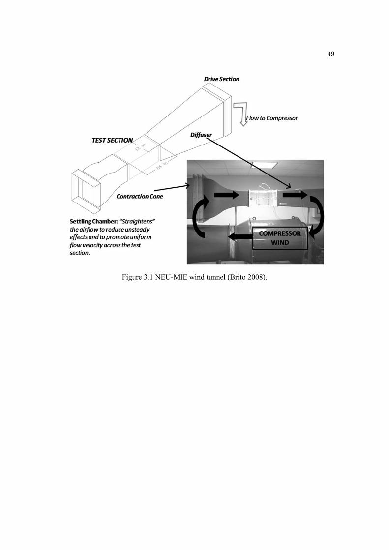
49
Figure 3.1 NEU-MIE wind tunnel (Brito 2008).
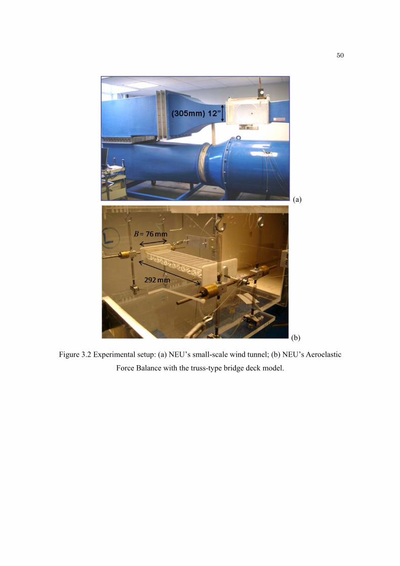
50
(a)
(b)
Figure 3.2 Experimental setup: (a) NEU’s small-scale wind tunnel; (b) NEU’s Aeroelastic
Force Balance with the truss-type bridge deck model.
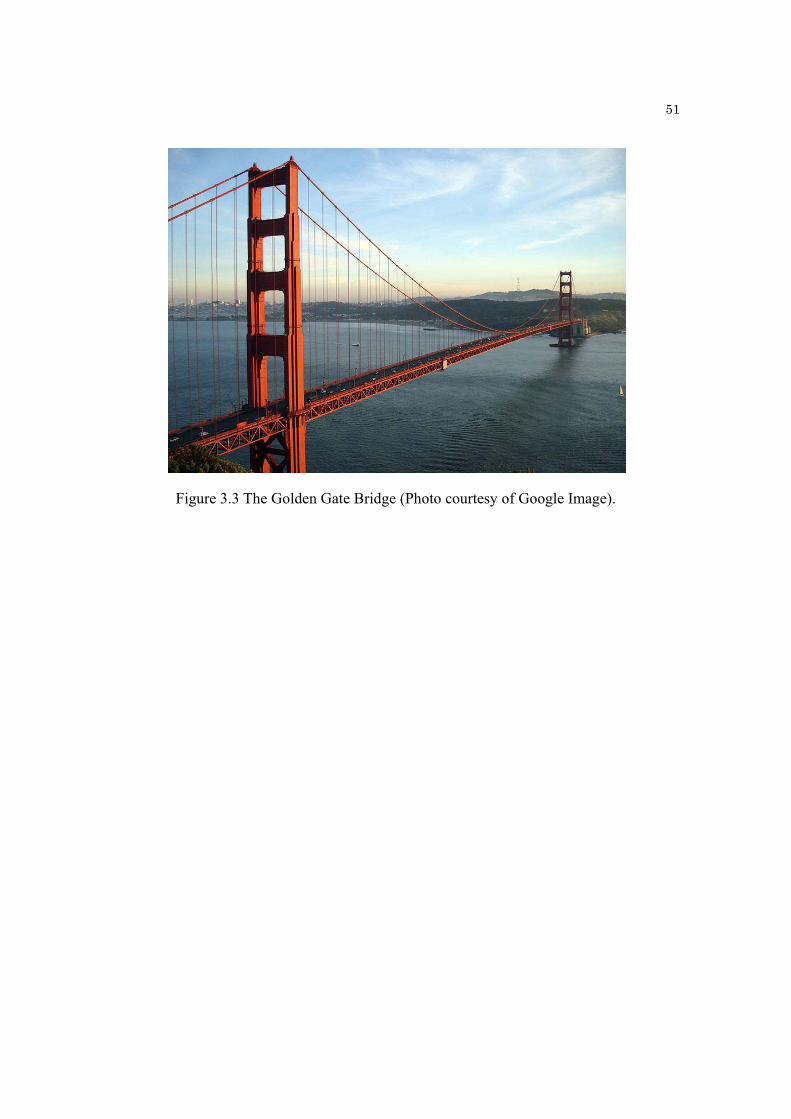
51
Figure 3.3 The Golden Gate Bridge (Photo courtesy of Google Image).
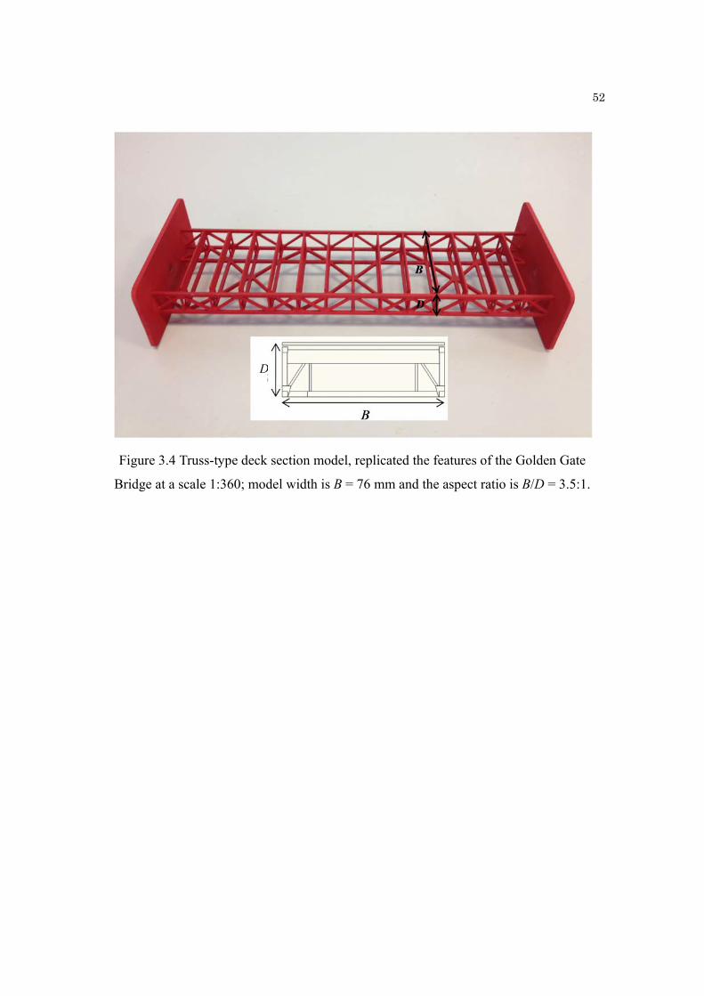
52
Figure 3.4 Truss-type deck section model, replicated the features of the Golden Gate
Bridge at a scale 1:360; model width is B = 76 mm and the aspect ratio is B/D = 3.5:1.
D
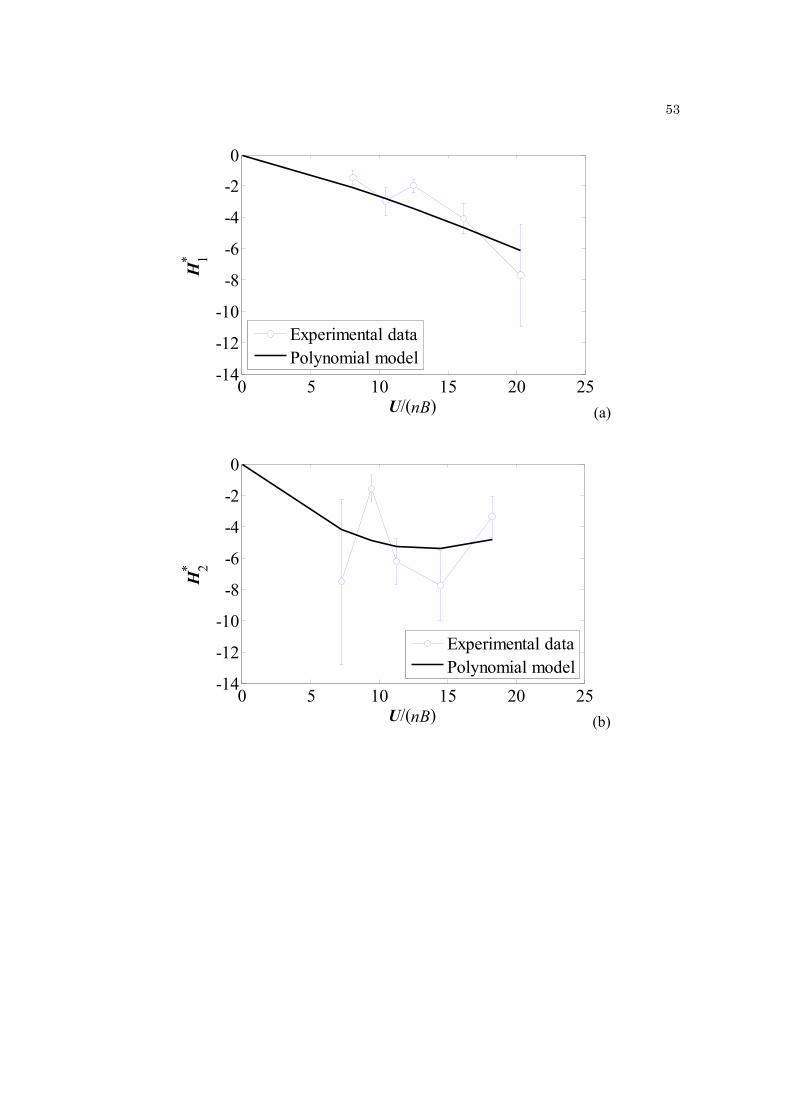
53
(a)
(b)
0 5 10 15 20 25-14
-12
-10
-8
-6
-4
-2
0
U/(nB)
H1*
Experimental dataPolynomial model
0 5 10 15 20 25-14
-12
-10
-8
-6
-4
-2
0
U/(nB)
H2*
Experimental dataPolynomial model

54
(c)
(d)
0 5 10 15 20 25-8
-6
-4
-2
0
2
4
6
U/(nB)
H3*
Experimental dataPolynomial model
0 5 10 15 20 25-12
-10
-8
-6
-4
-2
0
2
U/(nB)
H4*
Experimental dataPolynomial model
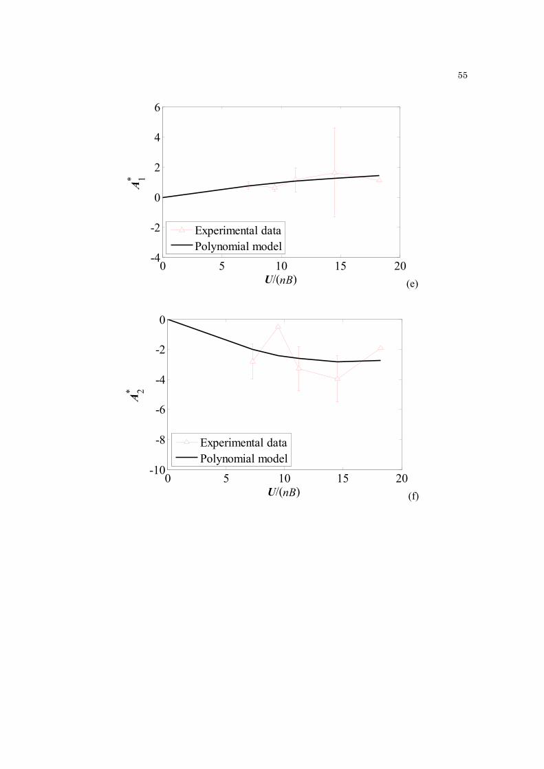
55
(e)
(f)
0 5 10 15 20-4
-2
0
2
4
6
U/(nB)
A1*
Experimental dataPolynomial model
0 5 10 15 20-10
-8
-6
-4
-2
0
U/(nB)
A2*
Experimental dataPolynomial model

56
(g)
(h)
Figure 3.5 Flutter derivatives of a truss-type section model with aspect ratio B/D= 3.5:1
measured at NEU: (a) H1*; (b) H2
*; (c) H3*; (d) H4
*; (e) A1*; (f) A2
*; (g) A3*; (h) A4
*.
0 5 10 15 20-6
-4
-2
0
2
4
U/(nB)
A3*
Experimental dataPolynomial model
0 5 10 15 20-4
-2
0
2
4
6
U/(nB)
A4*
Experimental dataPolynomial model
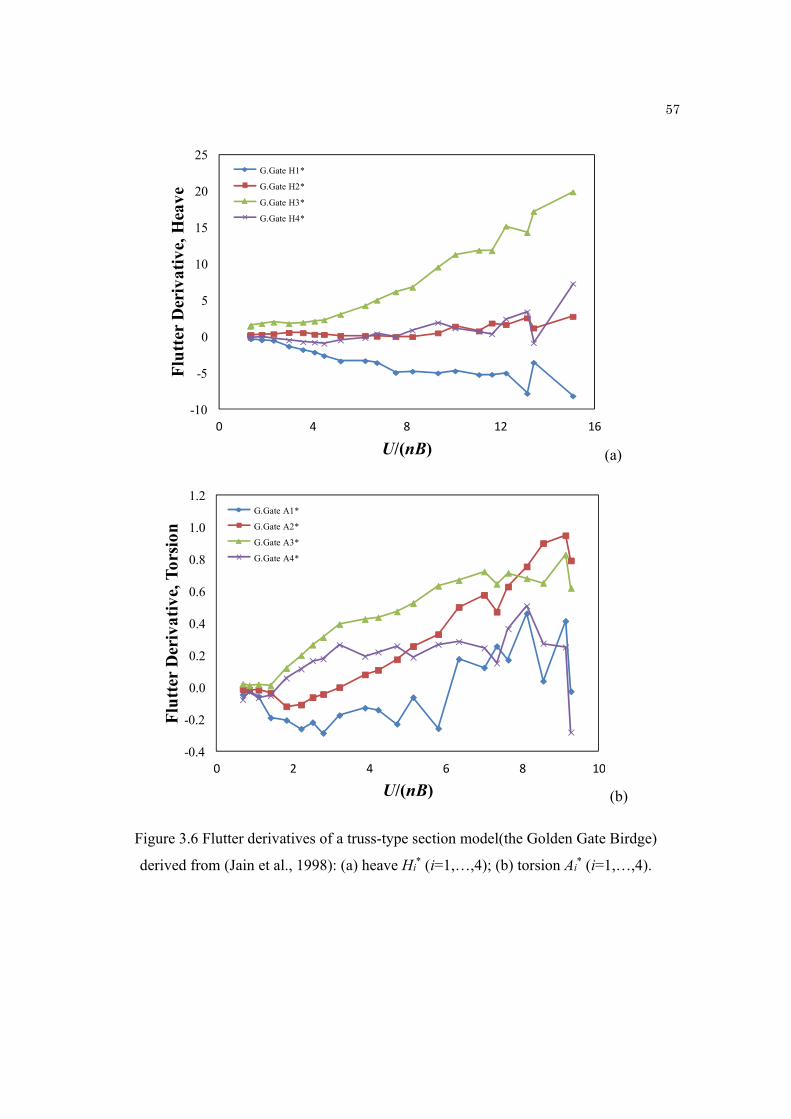
57
(a)
(b)
Figure 3.6 Flutter derivatives of a truss-type section model(the Golden Gate Birdge)
derived from (Jain et al., 1998): (a) heave Hi* (i=1,…,4); (b) torsion Ai
* (i=1,…,4).
-10
-5
0
5
10
15
20
25
0 4 8 12 16
Flu
tter
Der
ivat
ive,
Hea
ve
U/(nB)
G.Gate H1*
G.Gate H2*
G.Gate H3*
G.Gate H4*
-0.4
-0.2
0.0
0.2
0.4
0.6
0.8
1.0
1.2
0 2 4 6 8 10
Flu
tter
Der
ivat
ive,
Tor
sion
U/(nB)
G.Gate A1*
G.Gate A2*
G.Gate A3*
G.Gate A4*
58
Chapter 4
A Methodology for the Analysis of Long-Span Bridge
Buffeting Response, accounting for Variability in Flutter
Derivatives
4.1 Introduction
This chapter describes the development of a methodology for predicting the buffeting
response of a long-span bridge by Monte Carlo (MC) methods (Robert and Casella 2004;
Tempo et al. 2005). In the standard buffeting analysis (labeled as the “deterministic case” in
this work) the result is the value of the RMS dynamic response at a given wind speed. In the
proposed probabilistic setting (labeled as “statistical case” in this work) one estimates the
probability that a given threshold for the variance of the response is exceeded.
A Monte-Carlo-based methodology is proposed and implemented for predicting the
buffeting bridge response and for evaluating the variability due to uncertainty in the FDs
(“statistical buffeting” analysis). To accomplish these tasks, a second order polynomial
model (“model curve”) for the FD is utilized. The model curve is a second order polynomial

59
description of the FDs where uncertainty is associated with coefficient of the polynomial.
The coefficients of this polynomial are treated as random variables, whose probability
distribution is conditional on reduced wind speed. For computational reasons in subsequent
analysis, however, this dependency is neglected and the probability of these random
variables is treated as independent of the reduced wind speed. For analysis purposes the first
and second order statistics are estimated from experiments, treating all the wind speed data
as part of the same population.
A numerical procedure for multi-mode buffeting response (“deterministic case”) was
initially developed and its accuracy was validated by comparing with more reliable data from
the literature. In the standard multi-mode buffeting analysis, the power spectral density (PSD)
of the buffeting loads needs to be computed. This step, carried out by numerical integration,
is usually the “bottleneck” of the multi-mode buffeting analysis method in the modal space.
MC and Quasi-Monte-Carlo (QMC) methods were used to numerically compute the PSD of
the buffeting loads and to derive the root-mean-square (RMS) dynamic response of a long-
span bridge. A benchmark structure was utilized for this purpose (1,200 m suspension
bridge). A validation study was carried out by examining the performance of MC integration
methods using a series of standard buffeting analyses on the 1,200m bridge (Golden Gate
Bridge) and comparing the CPU time on a standard computer; also, the validation was
employed to determine the “optimal” number of sample points required by the MC and QMC
procedures in comparison with standard techniques for numerical integration. This part was
also based on a series of preliminary investigations (Caracoglia and Velazquez 2007).

60
Finally, the complete procedure (labeled as “MC-based methodology” in this
dissertation), which includes the probabilistic setting, is presented and implemented to
numerically evaluate for the probability of exceeding a set of pre-selected serviceability
thresholds, selected according to the RMS response of the deck as a function of mean wind
velocity and mean incident angle (skew wind). Such curves or surfaces were again derived
by MC sampling for two simulation examples, based on the same suspension bridge structure
(introduced above) and both literature data and measurements at NEU.
The MATLAB software environment was employed for coding purposes. The
detailed flowchart of the MC-based methodology for “statistical buffeting” analysis,
including the uncertainty in the FD, is shown in Fig. 4.1 and is described in the following
sub-sections.
4.2 Multi-Mode Buffeting Analysis (“Deterministic Case”)
The closed-form solution for multi-mode buffeting analysis by using the second order
polynomial model for FDs was developed in this work. One of the major problems to apply
the closed-form solution is related to the numerical integration of Eq. (2.24), which may
become computationally demanding and impractical in the context of statistical buffeting.
In order to overcome such limitations, Monte-Carlo and Quasi-Monte-Carlo methods
(Robert and Casella 2004; Tempo et al. 2005) were introduced and employed for numerical
integration.

61
4.2.1 Validation for Closed-Form Solution
The benchmark structure was derived from the dynamic behavior of a suspension bridge
with main span l = 1200 m, modeled after the Golden Gate Bridge in San Francisco,
California (USA). This bridge has a deck width B = 28 m, deck torsional inertia I0 = 4.4×10⁶
kg×m2/m (Jain et al. 1996). Modal structural damping ratio was selected as equal to 0.3%
for all modes as a deterministic constant by following the recommendations by Jain et al.
(1998) for this bridge. Lateral modes and responses were not analyzed, since the dynamic
bridge response for this bridge is mainly controlled by heaving and torsional motions (e.g.,
Jain et al, 1996). Flutter derivatives, Hi* and Ai
* along with the static coefficients of lift and
moment at α0 = 0° were reproduced from (Jain et al. 1998); the derivatives are shown in Fig.
3.6.
“Closed-form” (CF) estimation, which employs a standard integration algorithm (i.e.,
trapezoidal rule) for calculating the double integral in Eq. (2.24) to calculate the RMS
response based on standard multi-mode analysis, was employed for examination of the
computational efficiency of MC and QMC algorithms. The simulations included up to 10
fundamental structural deck modes of the benchmark structure. The natural frequencies and
mode types are shown in Table 4.1. Simplified (sinusoidal-like) mode shapes were assumed
and used to describe the main bridge motion (deck and cable vibration) shown in Fig. 4.3.
The CF solution was initially validated by comparison with the literature results,
provided by (Jain 1996) with 7 modes only. The RMS vibration was calculated for both
vertical σhh (Eq. 2.40a) and torsional σαα (Eq. 2.40c) responses at a quarter span of the bridge
deck x = l/4 and for wind speed at U = 22.2 m/s shown in Table 4.2. This bridge section was

62
selected since it corresponds to the anti-mode of the mode shapes in both the fundamental
vertical and torsional modes.
The vertical RMS response of the CF solution was in a good agreement with the
literature one, since the difference is equal to 4.1% in Table 4.2. Although the difference for
an overall torsional RMS displacement was quite large, equal to 182.1% in relative terms,
the result was accepted due to the fact that this value corresponds to an actual small rotation
in terms of degrees (i.e., angles 0.12° and 0.34° in Table 4.2) at full scale.
4.2.2 Monte-Carlo and Quasi-Monte-Carlo Methods
Monte-Carlo (MC) methods are a class of computational algorithms that rely on repeated
random sampling to compute their results. The MC numerical algorithm was employed to
compute the PSD of the buffeting loads Eq. (2.24) by integration and, later, to derive the
RMS response of the bridge Eq. (2.40) (Smith and Caracoglia 2011).
One of the major problems related to the numerical integration of Eq. (2.24), is the
fact that the integrand function needed to estimate Shh, Spp, Sαα in Eqs. (2.37–2.39) must be
evaluated numerically over a large portion of (xA, xB) for low frequency K. For low K the
whole (xA, xB) space contributes to the ( )i j
Q QS K function, whereas for moderate or large
frequencies the “non-zero part” of the integrand function concerns a tight zone, located along
the main diagonal in the (xA, xB) plane. This is a consequence of the decrease of coherence
with distance and frequency in the standard multi-mode formulation. Therefore, the
assessment of the integral for low-frequency structures becomes numerically demanding
since the resonant part of the loading is usually concentrated at low K.

63
In the MC-based approach for assessing the double integral in Eq. (2.24), two
samples of uniformly-distributed independent random variables are generated within an
interval of x, based on actual integration limits in Eq. (2.24) (0 ≤ x ≤ l) shown in Fig. 4.2(a).
These two sets of independent randomly-generated “points” (Robert and Casella 2004) are
used to find an approximation to the generic surface integral in Eq. (2.24). The use of Quasi-
Monte-Carlo (QMC) method was also investigated, as a “more deterministic” version of MC,
which is often preferred for reducing the variance of the estimated quantities and improving
the numerical efficiency (Tempo et al. 2005). In the QMC method the two-dimensional
coordinates of the “points” were chosen according to a deterministic criterion instead of a
“random selection” to distribute the integration points more evenly. The Halton sequence
(Tempo et al. 2005) was used in the QMC algorithm shown in Fig. 4.2(b).
An alternative way to reduce computational integration time would be possible if a
decomposition of the integral in Eq. (2.24) into “resonant” and “background” responses
(Davenport 1967) was used. This technique has been originally proposed in (Scanlan and
Jones 1990a) for long-span bridge aeroelastic analysis, providing approximate but still
acceptable results. Recently, this approach was re-proposed and used in a more generalized
form for bridge simulations (Denoël 2009; Gu and Zhou 2009), in an attempt to avoid
numerical integration issues. Nevertheless, the full integration is always more precise; it is
also preferable for the statistical buffeting analysis because accurate estimation of the
probability distribution of the error-contaminated RMS is crucial. Therefore, numerical
integration using MC and QMC methods has been chosen in this study.

64
4.2.3 Examination of the Computational Efficiency of the MC and QMC Methods for
Calculating the Double Integral in Eq. (2.24)
The accuracy and computational efficiency of the MC and QMC algorithms for double-
integration was assessed by repeating the estimation of the integral in Eq. (2.24) in the
absence of uncertainty in FDs (“deterministic case”). Simulations were repeated for various
MC integration points (NMC) to select an “optimal” value of NMC without compromising the
algorithmic accuracy. Two-mode analysis for the bridge example, simulating the structural
characteristics of existing bridge, was considered in this second investigation, restricted to
the first vertical and torsional skew-symmetric modes with frequencies nv1 = 0.087 Hz and
nt1 = 0.192 Hz (Mode n.2 in Fig. 4.3b and Mode n.8 in Fig. 4.3h).
Scatter plots, corresponding to 100 MC-based repeated estimates of the vertical and
torsional RMS responses as a function of NMC, were numerically evaluated. The performance
of the MC algorithm was also compared against the average relative run time (RT),
normalized to the value obtained for NMC = 50,000. The Coefficient of Variation (CoV) was
calculated and later employed as an indicator in the selection of the “optimal” NMC. The
maximum relative and bias errors (against the CF target value) were also calculated using
both MC and QMC methods.
Figure 4.3 shows the scatter plots corresponding to 100 repeated MC simulations
with the average RT also being indicated in the plots. The vertical (σhh in Fig. 4.4a) and
torsional (σαα in Fig. 4.4b) RMS responses of the deck of the simulated bridge for U = 22.2
m/s were compared to the target value at x = l/4.
In Fig. 4.5 the CoV, estimated for each sample population in Fig. 4.4 and
corresponding to each value of NMC, is shown in log-log scale. The CoV is a normalized

65
measure of dispersion in a distributed sample and was assessed as the ratio between the
standard deviation, σy,target, and mean of the sample, Yσ,mean.
As shown in Fig. 4.5(a), the CoV was very small for σhh, less than 1.4% in all cases.
The CoV for σαα was generally higher but very small for NMC > 10,000, less than 2.0%. In
Fig. 4.5(a) and Fig. 4.5(b), the decrement in the CoV was proportional to NMC on the log-log
chart with a constant negative slope in the curves; this behavior corresponds to a power-law
decrement for increasing NMC on a linear scale.
In Table 4.3 the maximum relative and bias errors for MC, estimated for each sample
population in Fig. 4.4 and corresponding to each value of NMC, are shown. The bias error
was estimated as the difference between the CF value of the RMS response and the mean of
the sample, σy,target - Yσ,mean. The relative error is the bias error divided by the mean of the
sample, σy,target / Yσ,mean. The relative errors were less than 0.7% for σhh at l/4 and -1.9% for
σαα, shown in Table 4.4, while they were almost negligible for larger sample sizes.
Tolerance intervals were employed to analyze the “fidelity” of the numerical
algorithms, as shown in Figs. 4.6 and 4.7. These tolerance limits were approximately
assessed assuming that the sample of RMS values follows a Gaussian distribution. In the
cause of a variable with Gaussian distribution and known population mean, μ, and standard
deviation, σ, the following tolerance limits can be used; μ ± z*σ. If z* = 1.96, these bounds
(covering the middle 95% of the population of observations) are essentially the confidence
intervals for a fixed proportion of the measurements (Walpole et al. 2002). When μ and σ are
unknown, which is typically the case, Eq. (4.1) can be applied.
(4.1) ,mean , target .yY k
66
The quantity k is the tolerance factor for a normal distribution. In this study, k is
defined such that there is a 99% confidence that the calculated tolerance limits will contain
at least 95% of the measurements, k = 2.36. The limiting confidence interval (e.g., 99%)
must be added to the statement since the bounds given by Eq. (4.1) cannot be expected to
contain any specified proportion (e.g., 95%) all of the time (Walpole et al. 2002). The
assumption of a normally-distributed population of σh and σα was used. Since the objective
was the section of an optimal sample size this hypothesis was accepted.
The tolerance interval results of are shown in Figs. 4.6 and 4.7. In both figures, the
horizontal axis represents the number of simulations conducted (i.e., 100 simulations) for a
given NMC, and the vertical axis is the RMS response. In each plot the tolerance intervals,
the target value (from CF simulations) and the results for each of the 100 simulations are
presented. All figures show a correlation between the number of integration points, NMC, and
the tolerance intervals, since the tolerance interval decreases as NMC increases. The tolerance
interval is approximately 9 times larger for NMC = 1,000 than it is for NMC = 100,000. The
benefit of using more integration points is clearly shown by the results of this investigation.
However, a smaller tolerance interval should not be the only criterion employed for the
selection of the optimal NMC. Figures 4.6 and 4.7 also suggest that, as the tolerance interval
decreases, the bias error can increase as the difference between the CF target value and the
estimated mean grows. Additionally, in Figs. 4.6(d) and 4.7(e) the tolerance limits no longer
contain the CF target value. This aspect must also be taken into consideration since the
overall goal of the MC simulations is to obtain results close to the CF “exact” value.

67
Figure 4.8 depicts the vertical (σhh in Fig. 4.8a) and torsional (σαα in Fig. 4.8b) RMS
responses of the same bridge example, using by QMC integration. Scatter plots and CoV of
σhh at l/4 correspond to 100 repeated simulations. The average RT was normalized to the
duration of the MC simulation with NMC = 50,000 for comparison with Fig. 4.4.
The CoV values in Fig. 4.9 (log-log scale) are much smaller than the ones observed
with the MC algorithm for both vertical and torsional response; however, the direct
proportionality on the log-log chart with a constant negative slope for all NQMC was not
observed. For example, the CoV for NQMC = 5,000 is less than 0.2%, which is clearly smaller
than approximately 0.5%, noticeable in Fig. 4.9(a) with NMC = 100,000. However, RT is
equal to 5.05, which is three times larger than the MC case with NMC = 100,000 (RT = 2.26).
The maximum relative and bias errors for QMC (Table 4.5) are shown. The relative
errors in the QMC case were less than 0.9% for σhh at l/4 and -3% for σαα, shown in Table
4.4. The relative and bias errors in the QMC case were larger than the ones in the MC case,
even though the QMC case had smaller CoVs. Tolerance intervals were also investigated
and are presented in Figs. 4.10 and 4.11.
From the interpretation of Fig. 4.4 through Fig. 4.11 it was concluded that QMC
integration, even with a medium sample size (NQMC > 10,000), was impractical because of
large RT. The QMC case with NQMC = 1,000 did not improve the numerical performance of
the standard algorithm in terms of CoV, with the RT being approximately eleven times larger
than the reference case with NMC = 1,000.
In the MC case the relative error of σhh consistently increases with an increment in
NMC; for the torsional response, the relative error also varies with NMC. The relationship

68
between the bias and the CoV was also utilized as an additional criterion for the selection of
the algorithm (MC or QMC). The QMC estimation showed smaller maximum relative errors
but higher bias errors (shown in Table 4.4).
As a consequence of the above observations, the MC integration algorithm was
selected in the subsequent stages of this study. By combining the results of Fig. 4.4 through
Fig. 4.7, NMC = 5,000 was recommended as the preferable choice for MC due to both
relatively small variance and good numerical efficiency. The computational time is
approximately one order of magnitude smaller than that of using a standard integration
algorithm (repeated trapezoidal rule).
4.3 Monte-Carlo-based Methodology for Buffeting Analysis Considering
Uncertainty in the Flutter Derivative (“Statistical Case”)
A Monte-Carlo-based methodology is proposed and implemented for predicting the
buffeting bridge response and for evaluating the variability due to uncertainty in the FDs
simulated by MC sampling. To accomplish these tasks, the second order polynomial model
(“model curve” in Eq. 3.1 and 3.2) for the FD is utilized, in which the coefficients of the
polynomial are random variables; more details can be found in Section 3.6.1.
In the MC-based methodology for buffeting analysis, the numerical procedure re-
calculates, at various wind speeds and skew wind angles, the buffeting loads by MC
sampling for each of the 5,000 realizations (e.g., the flowchart presented in Fig. 4.1). The
generalized power spectral density (PSD) of the buffeting loads is also calculated by MC
sampling, where a double integration (Eq. 2.24) is needed. Even though it is not necessary
to repeat the double integration for calculating the PSD of the buffeting loads, it is still

69
necessary to identify an efficient numerical procedure (Section 4.2.3) in order to be able to
generalize the method for future applications. In fact, extension of the method has been
investigated, in which also the effects of errors in the buffeting part of the loading must be
accounted for. These errors include, but are not limited to, simplifications in the modeling
of the wind turbulence spectrum, errors in the estimation of the span-wise loading parameters
Suu and Sww in Eq. (2.24). For more information on the effects of this category of errors, the
reader may refer to the recent publications in this area (Caracoglia 2008a; 2008b; 2011). In
the context of a future generalization of the method, in which the power spectral density of
the buffeting loading can become a random function in terms of K, repetition of the buffeting
loading estimation is required. Therefore, an efficient numerical procedure was needed.
In the proposed probabilistic setting (“statistical buffeting case”) one estimates the
probability that a given threshold for the variance of the response is exceeded. There are two
obvious formats to display the information that are useful in different ways. One way is to
plot the RMS value of buffeting response at a given confidence level of not being exceeded.
For example, Fig. 4.12 shows the RMS value for vertical buffeting response as a function of
wind speed at a given confidence level. More directly useful way for our purpose is to plot
the probability of exceedance at a given fixed RMS value as a function of wind speed. This
probability is designated as “threshold exceedance probability” (TEP) in this work, derived
by using a MC-based methodology with 5,000 sampling points (e.g., the flowchart presented
in Fig. 4.1) which projects the variability in the FD into the estimation of buffeting response.
The concept of using TEP was adopted from seismic engineering field (i.e., “fragility”).
70
Fragility analysis is a standardized methodology, utilized for performance-based
structural design. As a general statement, fragility curves measure (or quantify) the overall
structural vulnerability (Norton et al. 2008). The likelihood of structural damage due to
different “demand levels” – mean wind velocity levels in the case of wind engineering – is
usually expressed by a fragility curve (Saxena et al. 2000). A collection of these curves
describes the (conditional) probability of exceedance of representative structural response
indicators (“structural capacity”), corresponding to a specific feature of the dynamic
response at a given wind velocity (Bashor and Kareem 2007; Ellingwood 2000; Filliben et
al. 2002). A set of thresholds is usually selected to represent different levels of structural
performance derived from such indicators. As an example, in the case of a building these
indicators are either required or are prescribed by the designer, and can include inter-story
drift ratios, maximum lateral drift, and acceleration levels for occupant comfort (Bashor and
Kareem 2007; Filliben et al. 2002; Smith and Caracoglia 2011).
The TEP curves were developed in this dissertation by numerically deriving the
histogram of occurrences and the subsequent probability density function (PDF) of the RMS
dynamic response by a recursive procedure. The RMS response is a random variable in the
“probabilistic setting”. The probability of exceedance of pre-selected thresholds was later
calculated.
Equation 4.2 below relates the “loss of performance” of the structure, a bridge in this
study, which is the probability of exceeding of a threshold T, associated with the dynamic
response feature Y (performance indicator) at a given deck section for wind incidence angle
(θ) orthogonal to the longitudinal axis (initially assuming this response independent of wind
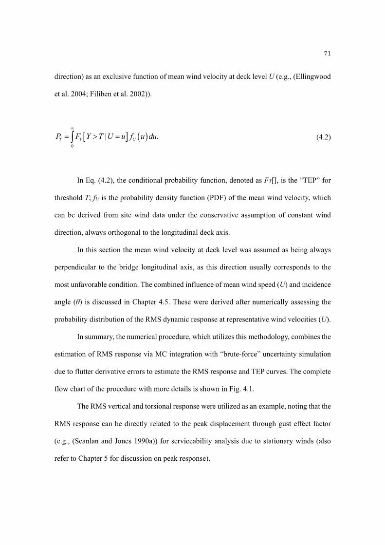
71
direction) as an exclusive function of mean wind velocity at deck level U (e.g., (Ellingwood
et al. 2004; Filiben et al. 2002)).
0
| .T T UP F Y T U u f u du
(4.2)
In Eq. (4.2), the conditional probability function, denoted as FT[], is the “TEP” for
threshold T; fU is the probability density function (PDF) of the mean wind velocity, which
can be derived from site wind data under the conservative assumption of constant wind
direction, always orthogonal to the longitudinal deck axis.
In this section the mean wind velocity at deck level was assumed as being always
perpendicular to the bridge longitudinal axis, as this direction usually corresponds to the
most unfavorable condition. The combined influence of mean wind speed (U) and incidence
angle (θ) is discussed in Chapter 4.5. These were derived after numerically assessing the
probability distribution of the RMS dynamic response at representative wind velocities (U).
In summary, the numerical procedure, which utilizes this methodology, combines the
estimation of RMS response via MC integration with “brute-force” uncertainty simulation
due to flutter derivative errors to estimate the RMS response and TEP curves. The complete
flow chart of the procedure with more details is shown in Fig. 4.1.
The RMS vertical and torsional response were utilized as an example, noting that the
RMS response can be directly related to the peak displacement through gust effect factor
(e.g., (Scanlan and Jones 1990a)) for serviceability analysis due to stationary winds (also
refer to Chapter 5 for discussion on peak response).
72
4.3.1 Description of the Bridge Example and RMS Threshold Levels (“Probabilistic
Setting”)
One bridge example was selected for “threshold exceedance probability” (TEP) analysis, the
same bridge model discussed in Section 4.2. Four-mode buffeting analysis was carried out
by considering the first two vertical (v1 and v2) and torsional modes (t1 and t2); it has
frequencies nv1 = 0.087 Hz and nv2 = 0.129 Hz, nt1 = 0.192 Hz and nt2 = 0.197 Hz. Simplified
(sinusoidal-like) mode shapes, shown in Fig 4.2(b, d, g and h) were used to describe the main
bridge motion (deck and cable vibration) in both models.
For example, as shown in Fig 4.2, the mode shapes of the vertical modes v1 and v2
were assumed as purely flexural, with shapes hv1(x) = sin(2πx/l) and hv2(x) = sin(πx/l), in
which l = 1,263 m is the central-span length for this bridge. Similarly, the shapes of torsional
modes t1 and t2 for the same model were simulated as purely torsional with αt1(x) = sin(2πx/l)
and αt2(x) = sin(πx/l).
The second order polynomial model (“model curve”) for flutter derivatives, proposed
in Section 3.4 to approximately account for effects of measurement errors in the FD, was
employed in the “statistical buffeting” analysis. Since eight flutter derivatives (H1*,…,H4
*
and A1*,…,A4
*) are measured in wind tunnel as a function of the reduced speed, UR = U/(nB)
= 2π/K, experimental data are usually available at discrete points on the UR (or K) axis. In
the TEP analysis, the coefficients of the model curves for each flutter derivative were
randomly perturbed to simulate the uncertainty in the FD; Hi*
= CiUR2 + Ci+1UR in Eq. (3.1)
with i=1,3,5,7 and Ai* = DjUR
2 + Dj+1UR in Eq. (3.2) with j=1,3,5,7.
The parameters of Hi* and Ai
* were assumed as a set of uncorrelated gamma-type
random variables. Description on the selection of this specific probability distribution may
73
be found in Section 3.4. The hypothesis of uncorrelated random variables is also described
in Section 3.4 The dispersion and shape parameters of the marginal probability of each
variable were associated with mean and standard deviation estimates of Hi* and Ai
*.
Three threshold levels were selected to derive the TEP curves. Table 4.5 shows the
threshold levels employed in the TEP analysis for σhh and σαα. Thresholds were based on a
median value of RMS displacements of the 5,000 buffeting analysis at wind velocity equal
to 20 m/s for the deck section at x = l/4, for example with T1 being equal to 50%, T2 equal to
100% and T3 equal to 150% of the corresponding the median value. For example, threshold
T2 corresponds to a dynamic displacement equal to 0.015D (i.e., D is being depth of the deck
equal to 7.83 m).
TEP analysis was carried out for the bridge example using flutter derivatives from
literature (Jain’s FD data) and flutter derivatives measured at Northeastern University (NEU).
4.3.2 TEP Curves using Literature Data
TEP curves, associated with the benchmark bridge model (Golden Gate Bridge) and based
on flutter derivatives reproduced from (Jain et al. 1998), were derived. The statistical
properties of the coefficients of the model curve were synthetically reproduced since no FD
error analysis was available. The coefficients of the Hi* and Ai
* model curves (Eqs. 3.1 and
3.2) were assumed as a set of uncorrelated gamma-type random variables. The dispersion
and shape parameters of the marginal probability of each variable were associated with the
mean and standard deviation estimates of Hi* and Ai.
For example, in Fig. 4.13 the Jain’s flutter derivatives H1* and A2
* are depicted; these
data were reproduced from the experiments described in (Jain 1996; Jain et al. 1996) and

74
from Fig. 3.6. The graphs also show the reference “model curves” based on the discrete data
points, assumed to be “average values” in the analysis. The dotted lines describe the upper
and lower limits of the reference curve that first statistics of the coefficients of the reference
curve was synthetically derived from such limits. Since no error analysis was carried out by
the investigators in their experiments, the variability (uncertainty) was indirectly estimated
in an approximate way, described above.
The TEP curves were calculated for both vertical and torsional vibrations at the
quarter span of the simulated bridge. The thresholds in Fig. 4.14(a) and Fig. 4.14(b) were
selected from Table 4.5. The TEP curves were developed by numerically deriving the
histogram of occurrences for each indicator at each wind velocity U, shown in Fig. 4.14(a)
and Fig. 4.14(b). The deterministic flutter velocity (DFV) without flutter derivative errors,
estimated as equal to 19.7 m/s, is also indicated a vertical dashed line.
In Fig. 4.14, the probability of exceeding T1, T2 or T3 increases as a result of a larger
perturbation (higher RMS response) for higher U. A small decrement in the TEP curves
related to T1 for U > 19.7 m/s in Fig. 4.14(a) may also be explained by potential inaccuracy
in the MC buffeting procedure in the proximity of flutter speed, as described below.
Beyond the deterministic flutter speed, the TEP curves are expressed as dotted lines
due to the onset of dynamic instability beyond a given critical velocity Ucr (deterministic
flutter velocity - DFV). Since the buffeting procedure numerically calculates the RMS
displacements of both vertical and torsional responses by spectral methods, it may fail by
predicting a finite RMS response at U beyond the velocity of the onset of flutter; finite
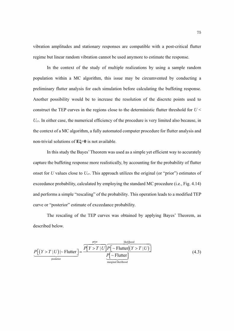
75
vibration amplitudes and stationary responses are compatible with a post-critical flutter
regime but linear random vibration cannot be used anymore to estimate the response.
In the context of the study of multiple realizations by using a sample random
population within a MC algorithm, this issue may be circumvented by conducting a
preliminary flutter analysis for each simulation before calculating the buffeting response.
Another possibility would be to increase the resolution of the discrete points used to
construct the TEP curves in the regions close to the deterministic flutter threshold for U <
Ucr. In either case, the numerical efficiency of the procedure is very limited also because, in
the context of a MC algorithm, a fully automated computer procedure for flutter analysis and
non-trivial solutions of Eξ=0 is not available.
In this study the Bayes’ Theorem was used as a simple yet efficient way to accurately
capture the buffeting response more realistically, by accounting for the probability of flutter
onset for U values close to Ucr. This approach utilizes the original (or “prior”) estimates of
exceedance probability, calculated by employing the standard MC procedure (i.e., Fig. 4.14)
and performs a simple “rescaling” of the probability. This operation leads to a modified TEP
curve or “posterior” estimate of exceedance probability.
The rescaling of the TEP curves was obtained by applying Bayes’ Theorem, as
described below.
P Y T |U |~ Flutter posterior
P Y T |U prior
P ~ Flutter Y T |U
likelihood
P ~ Flutter marginal likelihood
(4.3)
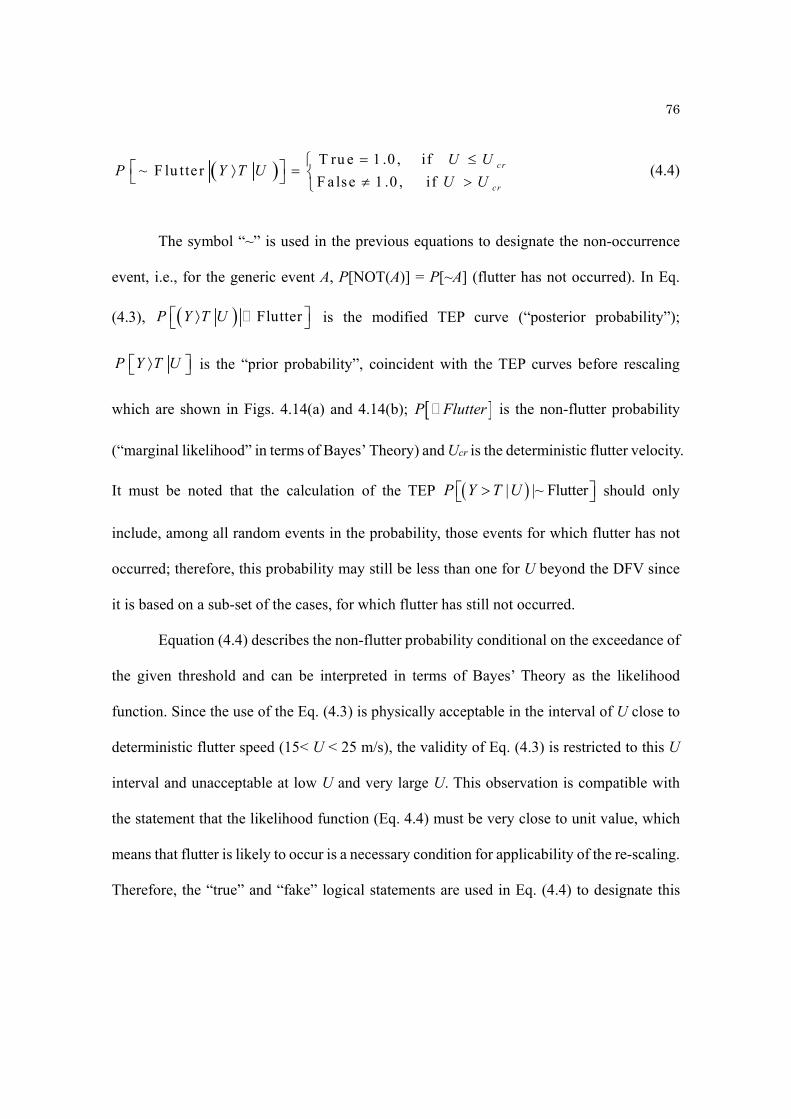
76
(4.4)
The symbol “~” is used in the previous equations to designate the non-occurrence
event, i.e., for the generic event A, P[NOT(A)] = P[~A] (flutter has not occurred). In Eq.
(4.3), is the modified TEP curve (“posterior probability”);
is the “prior probability”, coincident with the TEP curves before rescaling
which are shown in Figs. 4.14(a) and 4.14(b); is the non-flutter probability
(“marginal likelihood” in terms of Bayes’ Theory) and Ucr is the deterministic flutter velocity.
It must be noted that the calculation of the TEP | |~ FlutterP Y T U should only
include, among all random events in the probability, those events for which flutter has not
occurred; therefore, this probability may still be less than one for U beyond the DFV since
it is based on a sub-set of the cases, for which flutter has still not occurred.
Equation (4.4) describes the non-flutter probability conditional on the exceedance of
the given threshold and can be interpreted in terms of Bayes’ Theory as the likelihood
function. Since the use of the Eq. (4.3) is physically acceptable in the interval of U close to
deterministic flutter speed (15< U < 25 m/s), the validity of Eq. (4.3) is restricted to this U
interval and unacceptable at low U and very large U. This observation is compatible with
the statement that the likelihood function (Eq. 4.4) must be very close to unit value, which
means that flutter is likely to occur is a necessary condition for applicability of the re-scaling.
Therefore, the “true” and “fake” logical statements are used in Eq. (4.4) to designate this
T ru e 1 .0 , if ~ F lu tte r
F a lse 1 .0 , if c r
cr
U UP Y T U
U U
FlutterP Y T U
P Y T U
P Flutter
77
region of validity of Eq. (4.3). The rescaling, based on Eq. (4.3), is acceptable if the statement
in Eq. (4.4) is true and the conditional probability of flutter is 1.0.
In regions with crU U (DFV value) the rescaling is dubious since the assumption
on the hypothesis of a likelihood function close to the unit value is not satisfied; the practical
implication is that TEP greater than one may be observed.
Figure 4.15 depicts the procedure for rescaling based on Eq. (4.3). For example, the
discrete points on the initial curve (“prior” TEP) in Fig. 4.15(a) | ~ FlutterP Y T U ,
after multiplication by the likelihood function in Eq. (4.4), is divided by the marginal
likelihood function (i.e., the discrete points along the non-flutter probability
curve) in Fig. 4.15(b) to finally become Fig. 4.15(c) as a modified curve (“posterior” TEP).
Each curve in Fig. 4.14 was numerically evaluate by using the MC-based procedures and are
specific for the investigated case. The region of approximate validity of Eqs. (4.3-4.4) is
highlighted by a hatched area; it must be noted that the denominator in Eq. (4.3)
is strictly greater than zero in the region of validity (above 40% in Fig. 4.15(b)),
thereby confirming that | ~ FlutterP Y T U is not possible and that the proposed
rescaling is compatible with the assumptions.
The “posterior” TEP curves for T2, derived from Fig. 4.14 after rescaling, are shown
in Fig. 4.16.
4.3.3 TEP Curves using NEU’s Flutter Derivative Data
In order to further examine the performance of the MC-based methodology for TEP analysis,
flutter derivatives measured in the NEU’s wind tunnel were used. Eight flutter derivatives
P Flutter
P Flutter

78
(H1*,…,H4
* and A1*,…,A4
* in Fig. 3.5) were measured; the description of the wind tunnel
and experiments were presented in Chapter 3. Second-order statistical moments of flutter
derivatives were estimated from the wind tunnel measurements. Details may be found in
Section 3.6.
Structural properties of the model, the Golden Gate Bridge, were combined with
NEU’s experimental data in Fig. 3.5 to obtain a new set of TEP curves, based on threshold
levels in Table 4.5 shown in Fig. 4.17. For comparison purposes the T2 TEP curve, derived
from Jain’s flutter derivative data, was also reproduced from Figs. 4.16(a) and 4.16(b)
(dotted line, after the rescaling based on Eq. (4.3). These curves from Fig. 4.16 are shifted
to the right of the graph for vertical response and shifted to the left for torsion response. This
suggests that the variability in the FD play a significant role in the TEP analysis of this bridge
example and can reduce the dynamic performance, especially for the vertical DOF (Fig.
4.17a), if the FDs from literature were used.
4.4 Effect of Wind Directionality on “Statistical Buffeting” Response: TEP
Surfaces
In nature, the highest winds of record at a given site is very likely to be skew to the bridge
(Scanlan 1999). In this section, the multi-mode approach for wind direction orthogonal to
the deck axis was modified to account for directionality (θ), as originally proposed in
(Scanlan 1993). Background theory is described in Chapter 2. The latter approach enabled
the analysis of the combined influence of wind directionality and velocity, as these should
be more realistically used in serviceability analysis. This observation led to the derivation of
79
TEP surfaces (Filliben et al. 2002; Grigoriu 2002) as a function of various pre-selected
threshold levels.
Figure 4.18 shows the flutter derivative surfaces corresponding to T2 threshold in
Table 4.5 that include wind directionality affecting buffeting response of a bridge deck. In
Fig. 4.19, structural properties of the bridge were combined with NEU’s experimental data
in Fig. 3.5. A skew wind angle, varying from θ = –40° to θ = 40°, was considered in this
analysis.
Some influence on directionality can be observed in Fig. 4.18, especially for σαα.
Figures 4.18 and 4.19 confirm that the skew wind angle equal to zero degrees is the most
conservative assumption for both vertical and torsional buffeting responses.
4.5 Exploratory Performance Analysis on a Full-Scale Structure
In this section, the results in Section 4.4 were applied to the serviceability analysis of the
actual bridge structure, from which the structural and aeroelastic model was originally
derived. The structural performance was derived by extension of Eq. (4.2) to the case of
combined dependency on mean wind speed and direction. The exceedance probability and
“loss of performance” (PT) of the full-scale bridge structure was referred to TEP surfaces in
Fig. 4.18 and threshold T2. Equation (4.2) was re-written as follows:
180
180 0
| , , .T T UP F Y T U u f u dud
(4.5)
80
In Eq. (4.5), the conditional probability function, denoted as FT[], is the “TEP surface”
and fUΘ is the joint probability density function between mean wind velocity (U) and mean
wind incidence angle with respect to the axis of the bridge, which must be defined in the
interval –180° ≤ θ ≤ 180° (θ = 0° orthogonal to the bridge, θ = ±90° parallel to the bridge).
The wind data, used to estimate fU(U) and fθ(θ) given the assumption fUθ = fU·fθ, was
extracted from the historical records of a meteorological buoy close to the coast of California
in San Francisco (USA), which is part of the NOAA (National Oceanic and Atmospheric
Administration) system and National Data Buoy Center (NOAA Station 9414290, Latitude:
37.807 N, Longitude: 122.465 W, Shown in Fig. 4.20). This particular meteorological station
was selected because the prototype full-scale application (Golden Gate Bridge) is located in
proximity of the station. Data are available on-line from http://www.ndbc.noaa.gov/. Wind
speeds and directions at this station are measured using an anemometer located 7.3 meters
above mean sea level.
The histogram of annual maxima (“peak data” shown in Fig. 4.21) was derived from
the NOAA annual wind speed maxima over a 16-year period (1996-2011) and was employed
to evaluate fU(U). The annual wind speed maxima, obtained from the 16-year period, was
fitted to an Extreme Value Type-I distribution with two parameters, i.e., scale equal to 30.0
and location equal to 9.6 (Simiu and Scanlan 1996). The distribution of the mean yaw-wind
angle was based on a non-parametric model for the statistical distribution and derived from
the histogram of the mean wind direction (azimuthal) recorded by the sensor at elevation 7.3
m, postulating little effects of elevation on directionality. The azimuthal direction was later
converted to yaw-wind angle by using actual orientation of the bridge axis.
81
Table 4.6 summarizes the results of the performance analysis and shows the
estimation of the PT for both RMS vertical and torsional responses (dynamic component
only) for the bridge, evaluated at deck section x = l/4. These are respectively labeled as case
1 and case 2 in the table. In both cases the total probabilities of exceeding threshold T2 in
Table 4.5(a) are of the order of 2% by considering both wind speed and directionality.
Overall, the performance of the bridge is good from the point of view of the serviceability
standards. This analysis was completed by estimation of a “generalized safety index” for the
prototype application, defined as β = Ф-1(1 – PT) (Haldar and Mahadevan 2000) with Ф being
the standard normal cumulative density function.
The safety indices are also shown in Table 4.6; these should be interpreted as being
related to serviceability buffeting limit states. Reliability is acceptable, with safety indices
above 2 in both cases. Since effect of chord-wise aerodynamic admittance was not
considered in the model, a further reduction in the buffeting loading may possibly lead to a
decrement in PT; therefore, the results of Table 4.6 can be interpreted as a conservative
estimation of reliability and β.
Reliability against collapse (e.g., flutter) is not contemplated in this chapter, even
though it was indirectly included in the assessment of by Eq. (4.3).
4.6 Summary
The Monte-Carlo-based methodology for predicting the buffeting response of a long-span
bridge, including the uncertainty in the flutter derivative, was developed. The model curve
was utilized in the MC-based methodology; this curve is a second order polynomial
2 | ,TP Y Y U u

82
description of the FDs where uncertainty is associated with coefficient of the polynomial.
Statistical properties of the polynomial in the flutter derivatives were estimated both from
the literature and a set of measurements. Numerical procedures were coded and implemented
in MATLAB, using the methodology described in this chapter; the numerical program was
employed, to derive the dynamic response of two bridge structures at full scale.
The numerical results show that the RMS buffeting response of a long-span cable
supported bridge can be estimated (with sufficient accuracy to be practically useful) using a
second order polynomial description of the flutter derivatives. The uncertainty in these
derivatives in the model is captured by specifying the coefficients of the polynomial as a
vector of random variables having a specified mean and covariance (the values of these
properties used in the numerical analyses were obtained experimentally).
It is found that there is a significant computational advantage in using Monte-Carlo
methods for calculating a double integral that arises in the estimation of the generalized
buffeting loading, needed by the multi-mode buffeting analysis. The computational time is
approximately one order of magnitude smaller than that of using a standard integration
algorithm (repeated application of trapezoidal rule).
The results also suggest that the proposed MC-based methodology for buffeting
analysis might be used in conjunction with other dynamic indicators for analyzing the
serviceability in a full-scale structure (e.g., for comfort of the bridge users).
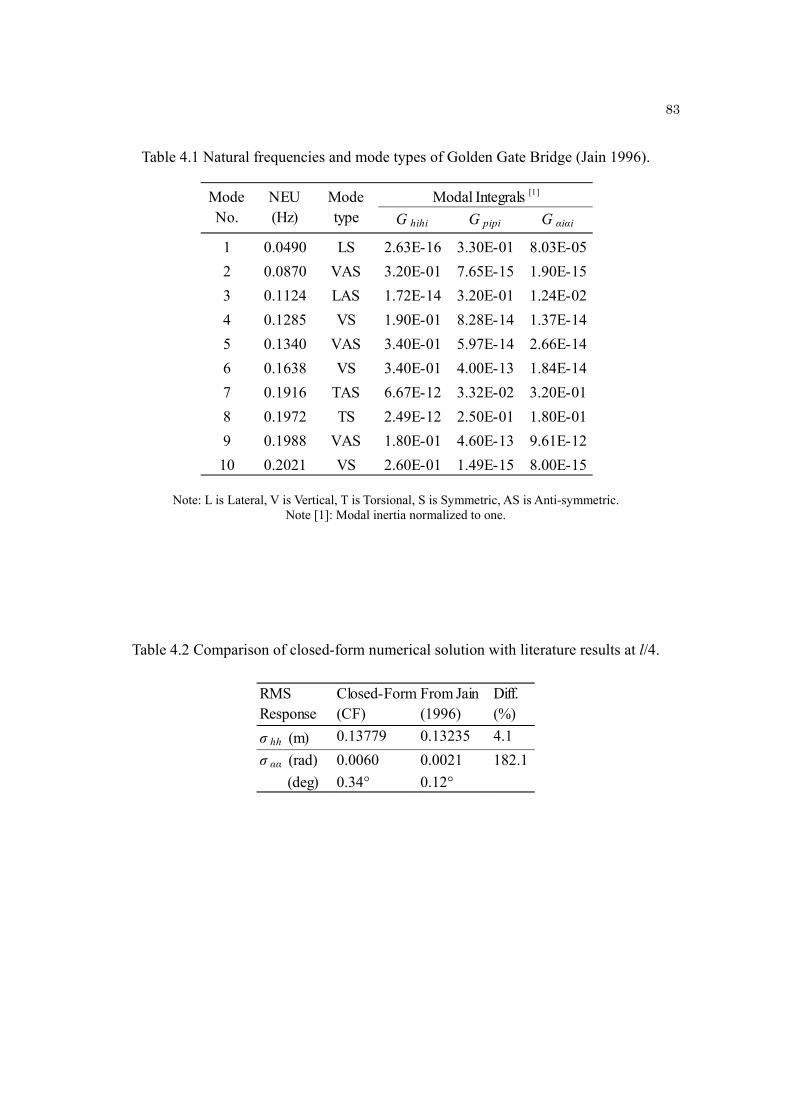
83
Table 4.1 Natural frequencies and mode types of Golden Gate Bridge (Jain 1996).
Note: L is Lateral, V is Vertical, T is Torsional, S is Symmetric, AS is Anti-symmetric. Note [1]: Modal inertia normalized to one.
Table 4.2 Comparison of closed-form numerical solution with literature results at l/4.
G hihi G pipi G αiαi
1 0.0490 LS 2.63E-16 3.30E-01 8.03E-05
2 0.0870 VAS 3.20E-01 7.65E-15 1.90E-15
3 0.1124 LAS 1.72E-14 3.20E-01 1.24E-02
4 0.1285 VS 1.90E-01 8.28E-14 1.37E-14
5 0.1340 VAS 3.40E-01 5.97E-14 2.66E-14
6 0.1638 VS 3.40E-01 4.00E-13 1.84E-14
7 0.1916 TAS 6.67E-12 3.32E-02 3.20E-01
8 0.1972 TS 2.49E-12 2.50E-01 1.80E-01
9 0.1988 VAS 1.80E-01 4.60E-13 9.61E-12
10 0.2021 VS 2.60E-01 1.49E-15 8.00E-15
NEU(Hz)
ModeNo.
Modetype
Modal Integrals [1]
σ hh (m) 0.13779 0.13235 4.1
σ αα (rad) 0.0060 0.0021 182.1
σαα (deg) 0.34° 0.12°
RMS Response
From Jain(1996)
Closed-Form(CF)
Diff.(%)

84
Table 4.3 Bias and relative errors in the MC case: (a) for heave σhh; (b) for torsion σαα.
(a)
(b)
N MC Bias × 10-4
(σy,target‐Yσ,mean)
Relative Error (%)
1,000 -0.23 -1.645,000 -0.27 -1.8710,000 -0.24 -1.6750,000 -0.24 -1.71100,000 -0.21 -1.49Note: y denotes either h or α
N MC Bias × 10-3
(σy,target‐Yσ,mean)
Relative Error (%)
1,000 0.52 0.395,000 0.62 0.4710,000 0.78 0.5950,000 0.82 0.62100,000 0.89 0.67Note: y denotes either h or α
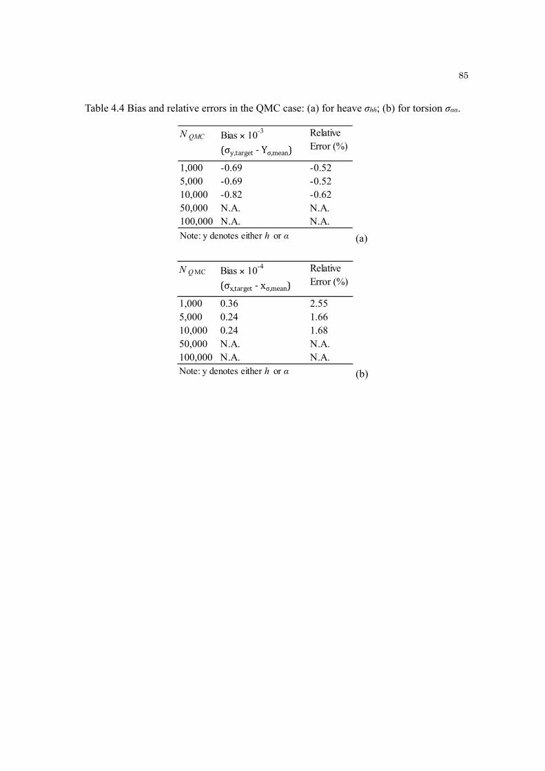
85
Table 4.4 Bias and relative errors in the QMC case: (a) for heave σhh; (b) for torsion σαα.
(a)
(b)
N QMC Bias × 10-3
(σy,target‐Yσ,mean)
Relative Error (%)
1,000 -0.69 -0.525,000 -0.69 -0.5210,000 -0.82 -0.6250,000 N.A. N.A.100,000 N.A. N.A.
Note: y denotes either h or α
N Q MC Bias × 10-4
(σx,target‐xσ,mean)
Relative Error (%)
1,000 0.36 2.555,000 0.24 1.6610,000 0.24 1.6850,000 N.A. N.A.100,000 N.A. N.A.Note: y denotes either h or α
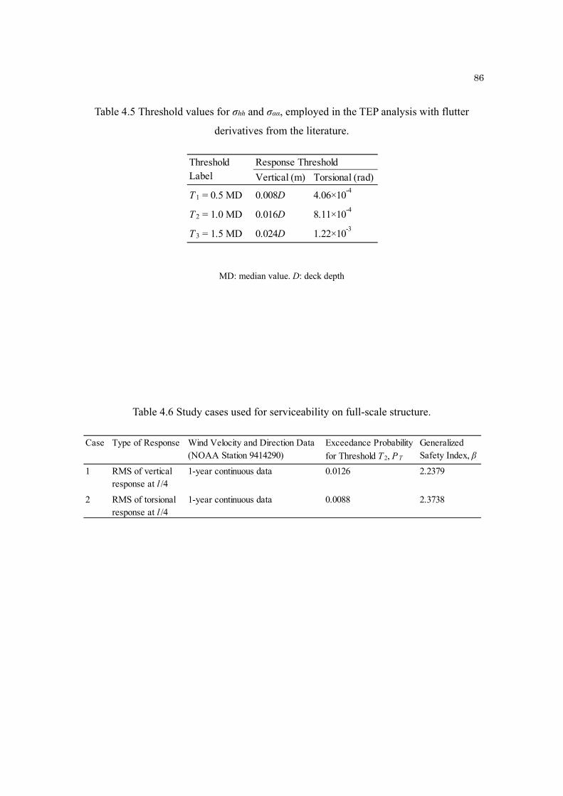
86
Table 4.5 Threshold values for σhh and σαα, employed in the TEP analysis with flutter
derivatives from the literature.
MD: median value. D: deck depth
Table 4.6 Study cases used for serviceability on full-scale structure.
Vertical (m) Torsional (rad)
T 1 = 0.5 MD 0.008D 4.06×10⁻⁴
T 2 = 1.0 MD 0.016D 8.11×10⁻⁴
T 3 = 1.5 MD 0.024D 1.22×10⁻³
ThresholdLabel
Response Threshold
Case Type of Response Wind Velocity and Direction Data(NOAA Station 9414290)
Exceedance Probability
for Threshold T 2, P T
Generalized Safety Index, β
1 RMS of vertical response at l /4
1-year continuous data 0.0126 2.2379
2 RMS of torsionalresponse at l /4
1-year continuous data 0.0088 2.3738

87
Figure 4.1 Flowchart describing the MC-based methodology for buffeting analysis.
F.E.MK, M, C(Deterministic)
Build deck section
Spectrum analysis of buffeting loads, SQQ
Formulate the Equation of Motion in the frequency domain and
incorporate the FD information
Estimate the RMS responseor
Test to obtain Data
Use Data to formulate a model for the FD that includes variability
Estimate the PSDof the response Sξξ
MC sampling of FD simulation
hh
Note: The numerical procedure depicted in the box is repeated for NMC times at various wind speeds and skew wind angles
Select wind speed (U) and skew angle (θ)
Model curves:Hi* = CjUR2+Cj+1URAi* = DjUR2+Dj+1UR
Calculate aeroelastic loads
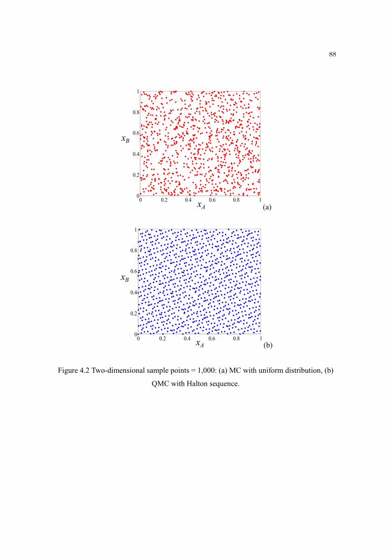
88
(a)
(b)
Figure 4.2 Two-dimensional sample points = 1,000: (a) MC with uniform distribution, (b)
QMC with Halton sequence.
0 0.2 0.4 0.6 0.8 10
0.2
0.4
0.6
0.8
1
xB
xA
0 0.2 0.4 0.6 0.8 10
0.2
0.4
0.6
0.8
1
xA
xB

89
(a)
(b)
(c)
0 200 400 600 800 1000 12000
0.2
0.4
0.6
0.8
1Mode n. 1
Mod
al A
mpl
itud
e
Longitudinal Abscissa
ph
0 200 400 600 800 1000 1200-1
-0.5
0
0.5
1Mode n. 2
Mod
al A
mpl
itud
e
Longitudinal Abscissa
ph
0 200 400 600 800 1000 1200-1
-0.5
0
0.5
1Mode n. 3
Mod
al A
mpl
itud
e
Longitudinal Abscissa
ph
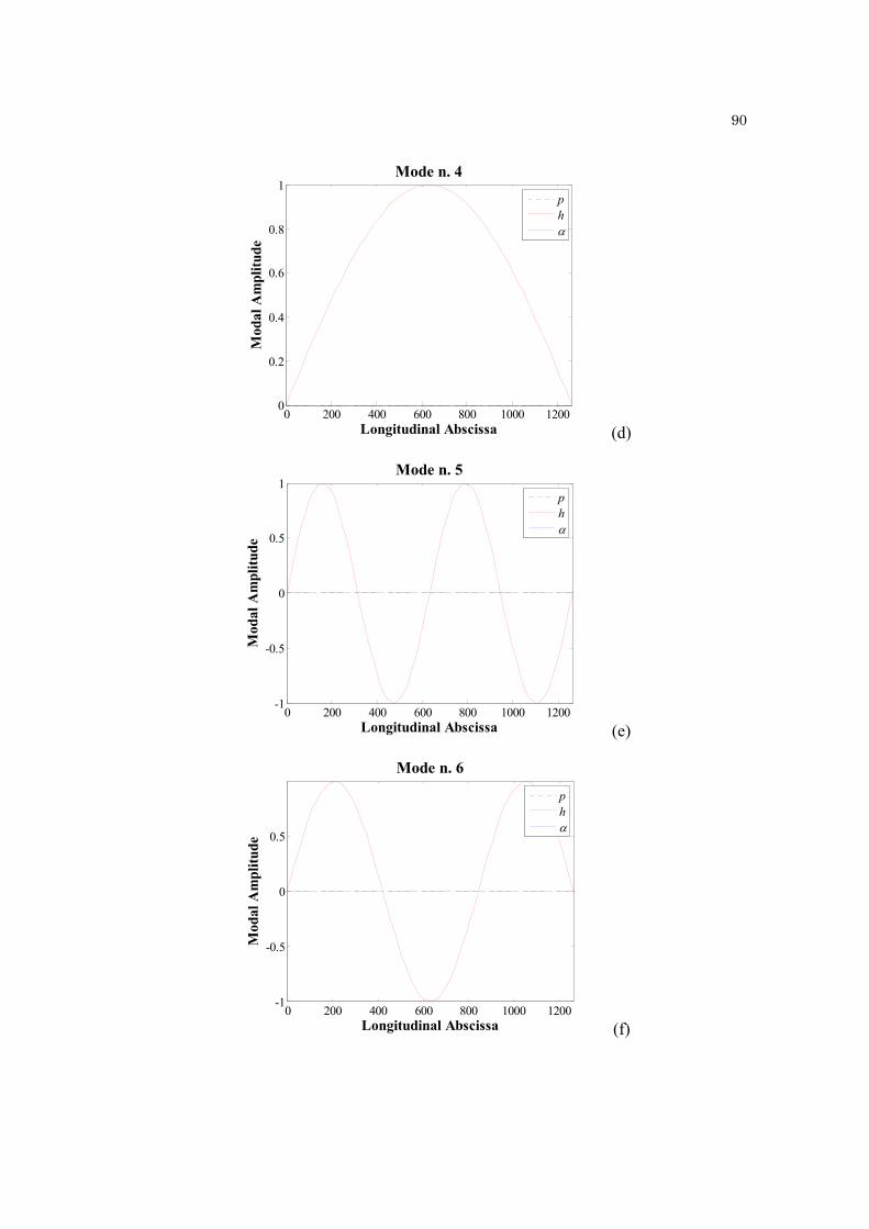
90
(d)
(e)
(f)
0 200 400 600 800 1000 12000
0.2
0.4
0.6
0.8
1Mode n. 4
Mod
al A
mpl
itud
e
Longitudinal Abscissa
ph
0 200 400 600 800 1000 1200-1
-0.5
0
0.5
1Mode n. 5
Mod
al A
mpl
itud
e
Longitudinal Abscissa
ph
0 200 400 600 800 1000 1200-1
-0.5
0
0.5
Mode n. 6
Mod
al A
mpl
itud
e
Longitudinal Abscissa
ph
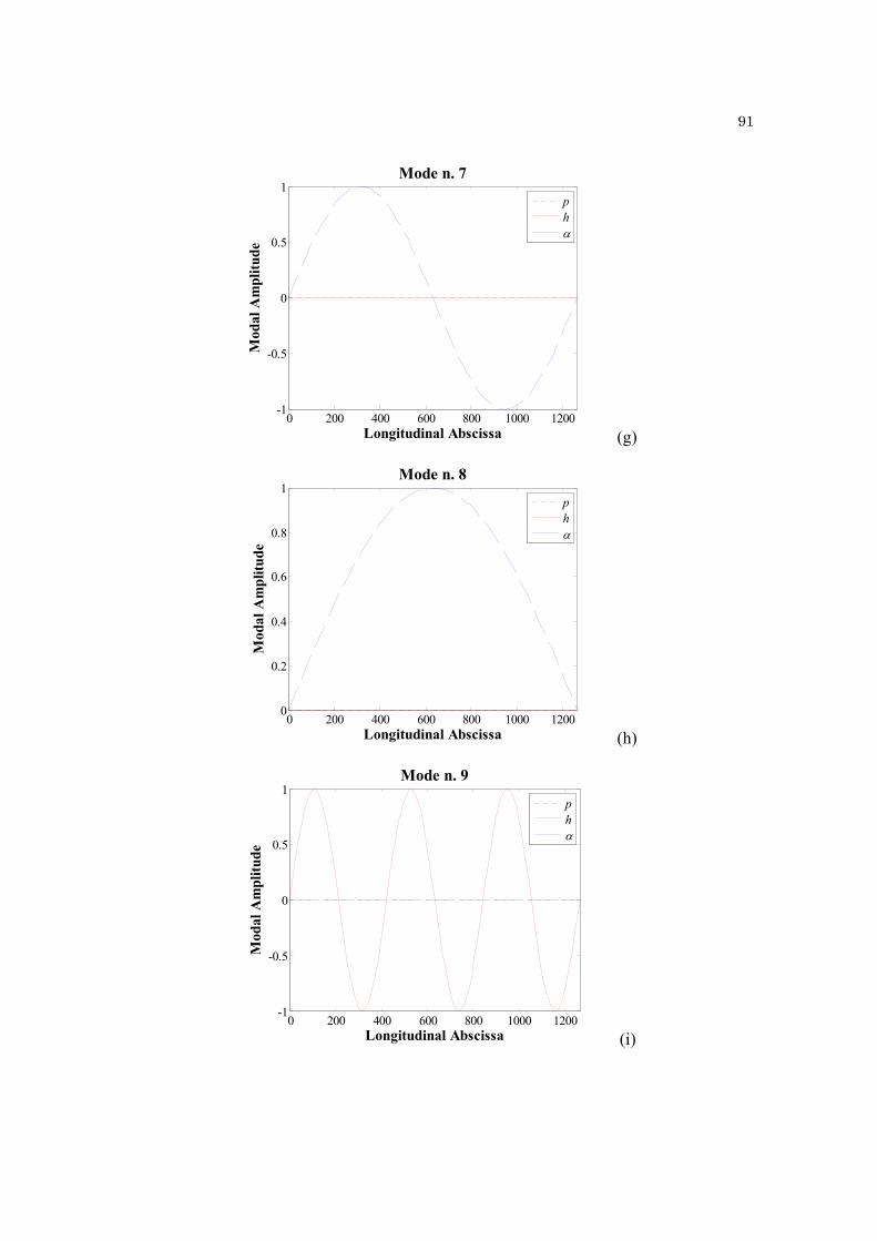
91
(g)
(h)
(i)
0 200 400 600 800 1000 1200-1
-0.5
0
0.5
1Mode n. 7
Mod
al A
mpl
itud
e
Longitudinal Abscissa
ph
0 200 400 600 800 1000 12000
0.2
0.4
0.6
0.8
1Mode n. 8
Mod
al A
mpl
itud
e
Longitudinal Abscissa
ph
0 200 400 600 800 1000 1200-1
-0.5
0
0.5
1Mode n. 9
Mod
al A
mpl
itud
e
Longitudinal Abscissa
ph

92
(j)
Figure 4.3 Ten simplified (sinusoidal-like) mode shapes used in the multi-mode buffeting
analysis: (a) LS, 0.049 Hz; (b) VAS, 0.087Hz; (c) LAS, 0.112 Hz; (d) VS, 0.129 Hz; (e)
VAS, 0.134 Hz; (f) VS, 0.164 Hz; (g) TAS, 0.192 Hz; (h) TS, 0.197 Hz; (i) VAS, 0.199 Hz;
(j) VS, 0.202 Hz. (Note: L is Lateral, V is Vertical, T is Torsional, S is Symmetric, AS is
Anti-symmetric).
0 200 400 600 800 1000 1200-1
-0.5
0
0.5
1Mode n. 10
Mod
al A
mpl
itud
e
Longitudinal Abscissa
ph
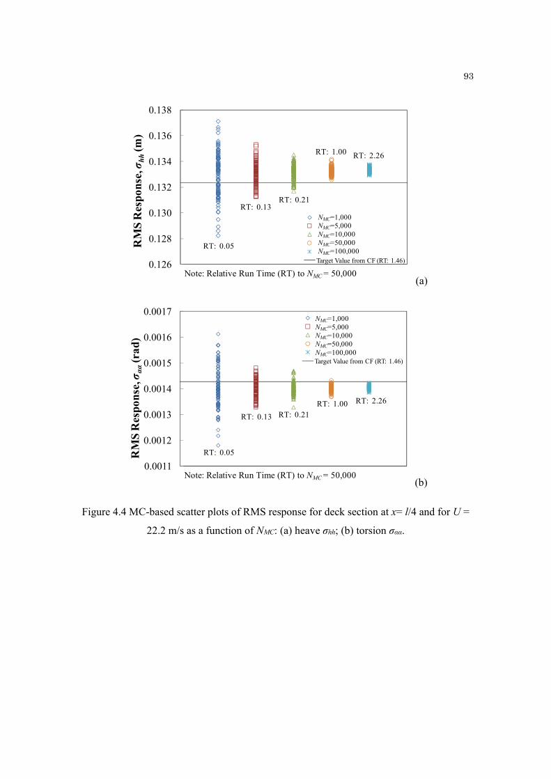
93
(a)
(b)
Figure 4.4 MC-based scatter plots of RMS response for deck section at x= l/4 and for U =
22.2 m/s as a function of NMC: (a) heave σhh; (b) torsion σαα.
0.126
0.128
0.130
0.132
0.134
0.136
0.138
RM
S R
espo
nse
, σhh
(m)
NMC= 1,000NMC = 5,000NMC = 10,000NMC = 50,000NMC = 100,000Target Value from CF (RT: 1.46)
RT: 0.05
RT: 0.13RT: 0.21
RT: 1.00 RT: 2.26
Note: Relative Run Time (RT) to NMC = 50,000
NMC=1,000NMC=5,000NMC=10,000NMC=50,000NMC=100,000
0.0011
0.0012
0.0013
0.0014
0.0015
0.0016
0.0017
RM
S R
espo
nse
, σαα
(rad
)
NMC = 1,000NMC = 5,000NMC = 10,000NMC = 50,000NMC = 100,000Target Value from CF (RT: 1.46)
RT: 0.05
RT: 0.13 RT: 0.21RT: 1.00 RT: 2.26
Note: Relative Run Time (RT) to NMC = 50,000
NMC=1,000NMC=5,000NMC=10,000NMC=50,000NMC=100,000
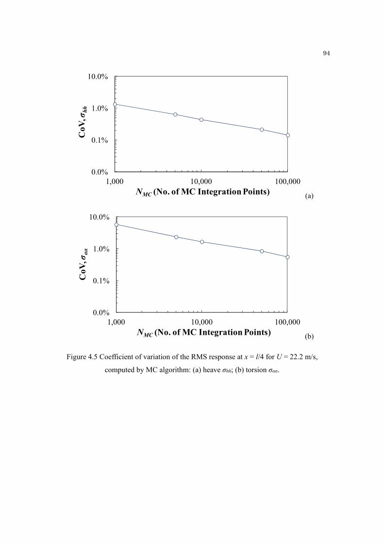
94
(a)
(b)
Figure 4.5 Coefficient of variation of the RMS response at x = l/4 for U = 22.2 m/s,
computed by MC algorithm: (a) heave σhh; (b) torsion σαα.
0.0%
0.1%
1.0%
10.0%
1,000 10,000 100,000
CoV
, σhh
NMC (No. of MC Integration Points)
0.0%
0.1%
1.0%
10.0%
1,000 10,000 100,000
CoV
, σαα
NMC (No. of MC Integration Points)
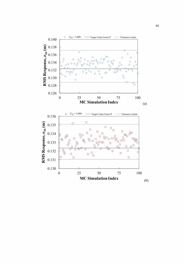
95
(a)
(b)
0.126
0.128
0.130
0.132
0.134
0.136
0.138
0.140
0 25 50 75 100
RM
S R
esp
onse
, σhh
(m)
MC Simulation Index
NMC = 1,000 Target Value from CF Tolerance LimitsNMC = 1,000
0.130
0.131
0.132
0.133
0.134
0.135
0.136
0 25 50 75 100
RM
S R
esp
onse
, σhh
(m)
MC Simulation Index
NMC = 5,000 Target Value from CF Tolerance LimitsNMC = 5,000
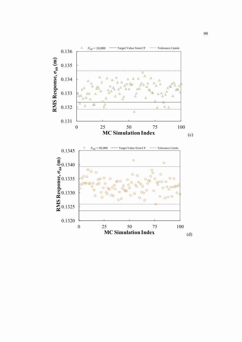
96
(c)
(d)
0.131
0.132
0.133
0.134
0.135
0.136
0 25 50 75 100
RM
S R
espo
nse,
σhh
(m)
MC Simulation Index
NMC = 10,000 Target Value from CF Tolerance LimitsNMC = 10,000
0.1320
0.1325
0.1330
0.1335
0.1340
0.1345
0 25 50 75 100
RM
S R
esp
onse
, σhh
(m)
MC Simulation Index
NMC = 50,000 Target Value from CF Tolerance LimitsNMC = 50,000

97
(e)
Figure 4.6 Tolerance intervals for vertical RMS response (σhh) of 100 MC simulations: (a)
NMC = 1,000; (b) NMC = 5,000; (c) NMC = 10,000; (d) NMC = 50,000; (e) NMC = 100,000.
0.1320
0.1325
0.1330
0.1335
0.1340
0.1345
0 25 50 75 100
RM
S R
espo
nse,
σhh
(m)
MC Simulation Index
NMC = 100,000 Target Value from CF Tolerance LimitsNMC = 100,000

98
(a)
(b)
0.00110
0.00120
0.00130
0.00140
0.00150
0.00160
0.00170
0 25 50 75 100
RM
S R
esp
onse
, σαα
(rad
.)
MC Simulation Index
NMC = 1,000 Target Value from CF Tolerance LimitsNMC = 1,000
0.00125
0.00130
0.00135
0.00140
0.00145
0.00150
0.00155
0 25 50 75 100
RM
S R
esp
onse
, σαα
(rad
)
MC Simulation Index
NMC = 5,000 Target Value from CF Tolerance LimitsNMC = 5,000

99
(c)
(d)
0.00130
0.00133
0.00136
0.00139
0.00142
0.00145
0.00148
0.00151
0 25 50 75 100
RM
S R
esp
onse
, σαα
(rad
.)
MC Simulation Index
NMC = 10,000 Target Value from CF Tolerance LimitsNMC = 10,000
0.00134
0.00136
0.00138
0.00140
0.00142
0.00144
0.00146
0 25 50 75 100
RM
S R
esp
onse
, σαα
(rad
.)
MC Simulation Index
NMC = 50,000 Target Value from CF Tolerance LimitsNMC = 50,000
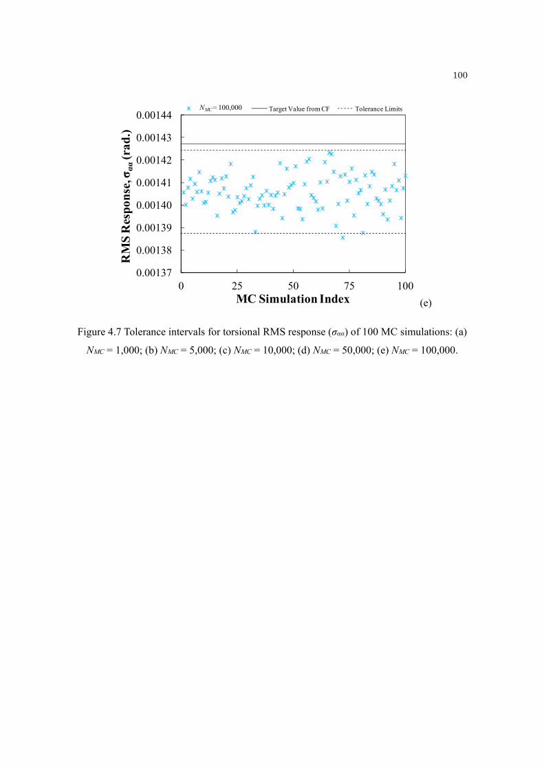
100
(e)
Figure 4.7 Tolerance intervals for torsional RMS response (σαα) of 100 MC simulations: (a)
NMC = 1,000; (b) NMC = 5,000; (c) NMC = 10,000; (d) NMC = 50,000; (e) NMC = 100,000.
0.00137
0.00138
0.00139
0.00140
0.00141
0.00142
0.00143
0.00144
0 25 50 75 100
RM
S R
esp
onse
, σαα
(rad
.)
MC Simulation Index
NMC = 100,000 Target Value from CF Tolerance LimitsNMC = 100,000
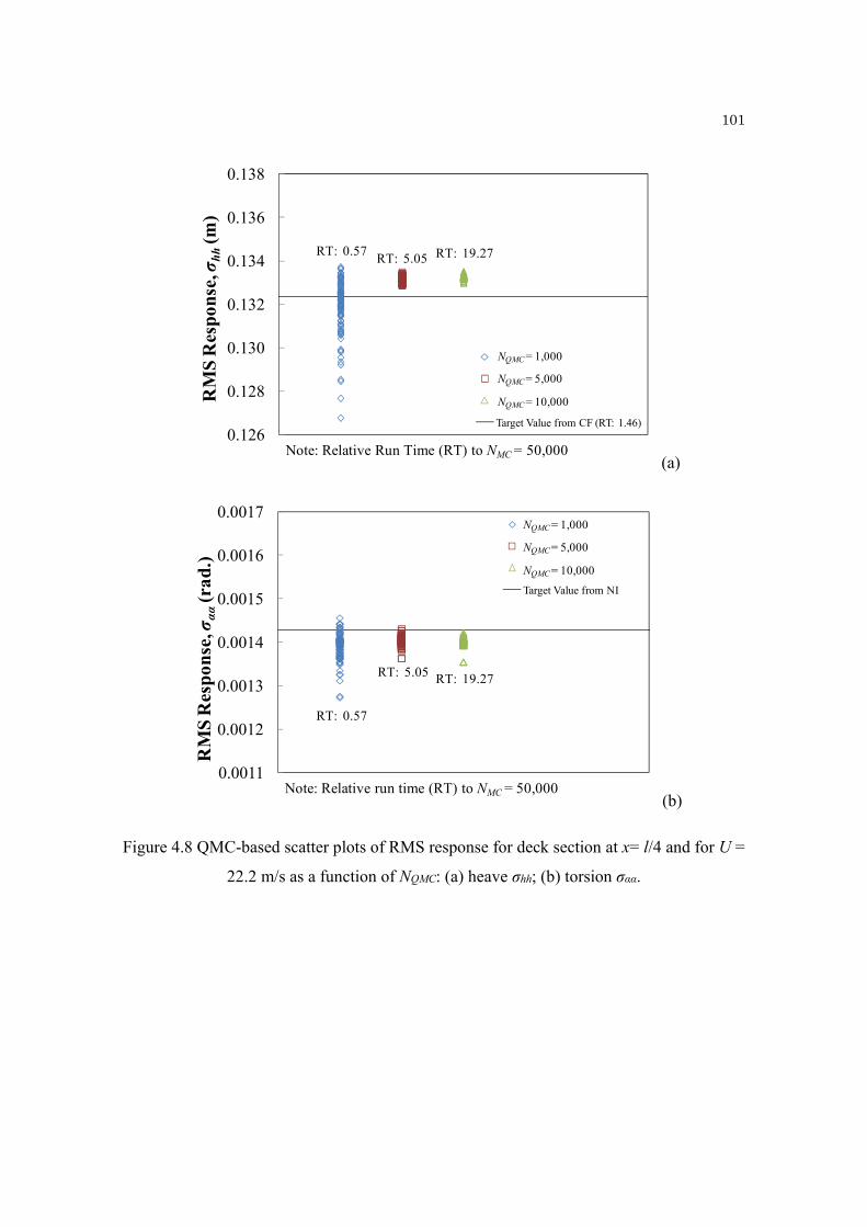
101
(a)
(b)
Figure 4.8 QMC-based scatter plots of RMS response for deck section at x= l/4 and for U =
22.2 m/s as a function of NQMC: (a) heave σhh; (b) torsion σαα.
0.126
0.128
0.130
0.132
0.134
0.136
0.138
RM
S R
esp
onse
, σhh
(m)
NQMC = 1,000
NQMC = 5,000
NQMC = 10,000
Target Value from CF (RT: 1.46)
RT: 0.57RT: 5.05 RT: 19.27
Note: Relative Run Time (RT) to NMC = 50,000
NQMC = 1,000
NQMC = 5,000
NQMC = 10,000
0.0011
0.0012
0.0013
0.0014
0.0015
0.0016
0.0017
RM
S R
esp
onse
, σαα
(rad
.)
NQMC = 1,000
NQMC = 5,000
NQMC = 10,000
Target Value from NI
RT: 0.57
RT: 5.05 RT: 19.27
Note: Relative run time (RT) to NMC = 50,000
NQMC = 1,000
NQMC = 5,000
NQMC = 10,000

102
(a)
(b)
Figure 4.9 Coefficient of variation of the RMS response at x = l/4 for U = 22.2 m/s,
computed by QMC algorithm: (a) heave σhh; (b) torsion σαα.
0.0%
0.1%
1.0%
10.0%
1,000 10,000 100,000
Co
V, σhh
NQMC (No. of QMC Integration Points)
0.1%
1.0%
10.0%
1,000 10,000 100,000
CoV
, σαα
NQMC (No. of QMC Integration Points)
103
(a)
(b)
0.126
0.128
0.130
0.132
0.134
0.136
0.138
0.140
0 25 50 75 100
RM
S R
esp
onse
, σhh
(m)
QMC Simulation Index
NMC = 1,000 Target Value from CF Tolerance LimitsNQMC = 1,000
0.130
0.131
0.132
0.133
0.134
0.135
0.136
0 25 50 75 100
RM
S R
esp
onse
, σhh
(m)
QMC Simulation Index
NMC = 5,000 Target Value from CF Tolerance LimitsNQMC = 5,000

104
(c)
Figure 4.10 Tolerance intervals for vertical RMS response of 100 MC simulations (σhh): (a)
NQMC = 1,000; (b) NQMC = 5,000; (a) NQMC = 10,000.
0.131
0.132
0.133
0.134
0.135
0.136
0 25 50 75 100
RM
S R
esp
onse
, σhh
(m)
QMC Simulation Index
NMC = 10,000 Target Value from CF Tolerance LimitsNQMC = 10,000
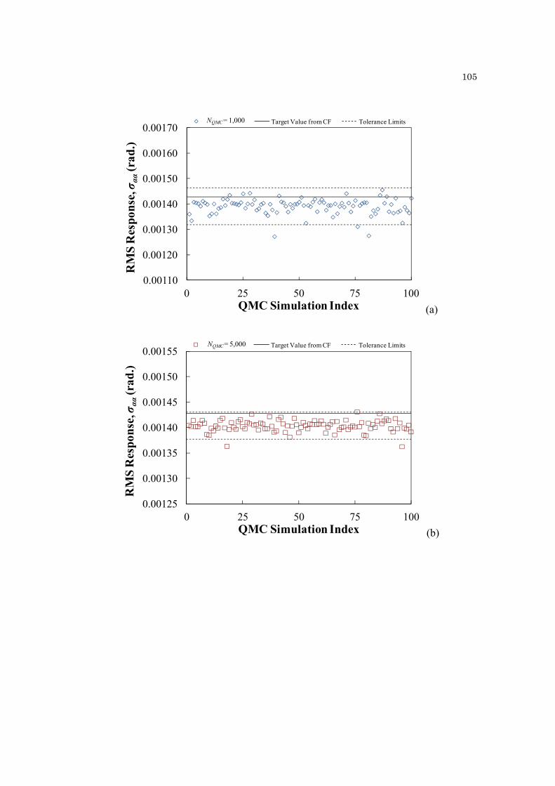
105
(a)
(b)
0.00110
0.00120
0.00130
0.00140
0.00150
0.00160
0.00170
0 25 50 75 100
RM
S R
esp
onse
, σαα
(rad
.)
QMC Simulation Index
NMC = 1,000 Target Value from CF Tolerance LimitsNQMC = 1,000
0.00125
0.00130
0.00135
0.00140
0.00145
0.00150
0.00155
0 25 50 75 100
RM
S R
espo
nse
, σαα
(rad
.)
QMC Simulation Index
NMC = 5,000 Target Value from CF Tolerance LimitsNQMC = 5,000
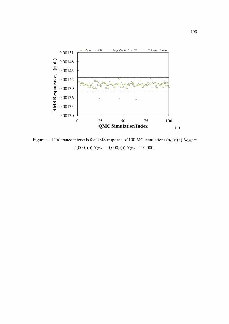
106
(c)
Figure 4.11 Tolerance intervals for RMS response of 100 MC simulations (σαα): (a) NQMC =
1,000; (b) NQMC = 5,000; (a) NQMC = 10,000.
0.00130
0.00133
0.00136
0.00139
0.00142
0.00145
0.00148
0.00151
0 25 50 75 100
RM
S R
esp
onse
, σαα
(rad
.)
QMC Simulation Index
NMC = 10,000 Target Value from CF Tolerance LimitsNQMC = 10,000
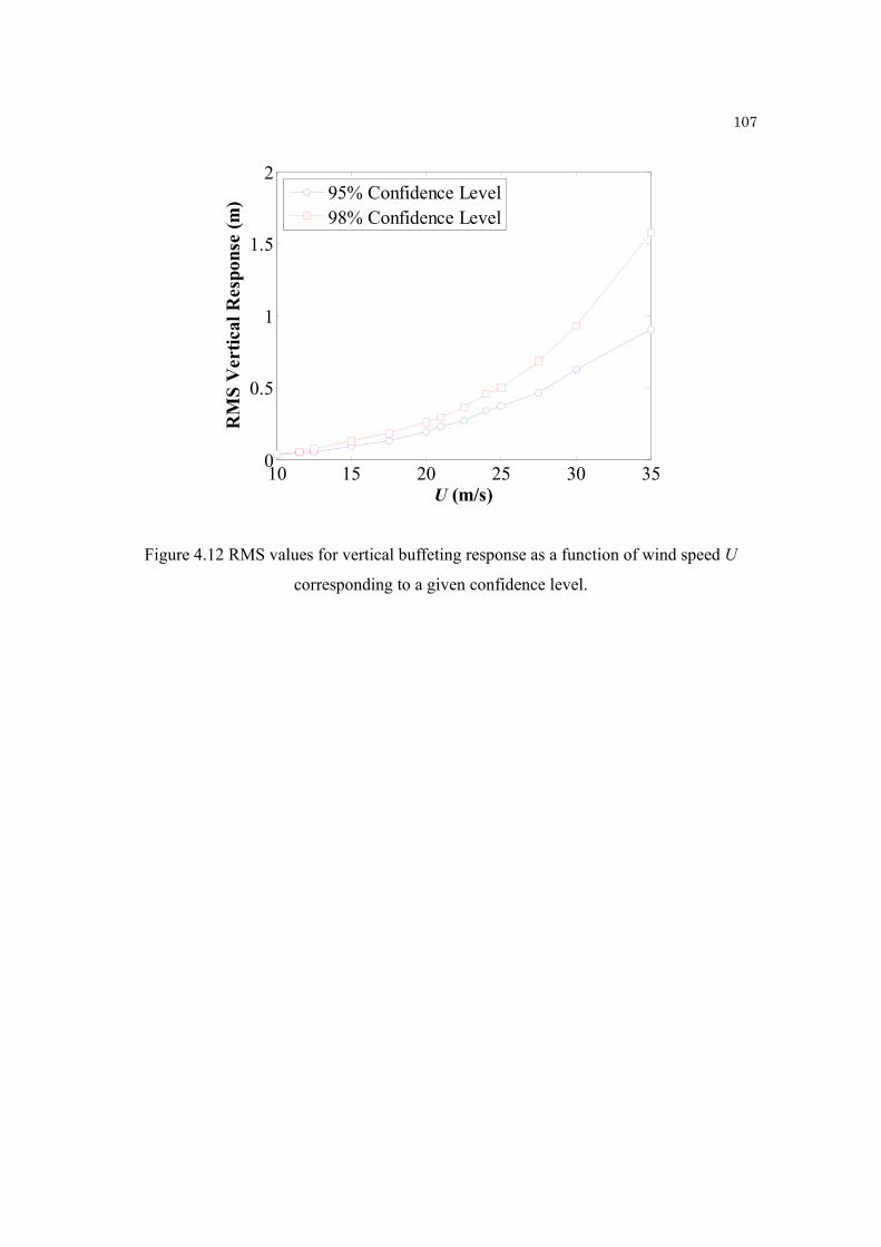
107
Figure 4.12 RMS values for vertical buffeting response as a function of wind speed U
corresponding to a given confidence level.
10 15 20 25 30 350
0.5
1
1.5
2
RM
S V
erti
cal R
espo
nse
(m)
U (m/s)
95% Confidence Level98% Confidence Level

108
(a)
(b)
Figure 4.13 Flutter derivatives H1* (a) and A2
* (b) of the Golden-Gate Bridge girder with
aspect ratio B/D = 3.5:1. Data sets were reproduced from (Jain 1996; Jain et al. 1996) with
α0=0°. The (“reference”) coefficients of the “Polynomial Model” were derived by
regression of the data sets, according to Eqs. (3.1) and (3.2). Tolerance limits (dashed lines)
were based on approximate evaluation of one standard deviation.
-7.0
-6.0
-5.0
-4.0
-3.0
-2.0
-1.0
0.0
0 2 4 6 8 10 12
Flu
tter
Der
ivat
ive,
Lif
t
Reduced Velocity
G.Gate H1*Reference
-0.2
0.0
0.2
0.4
0.6
0.8
1.0
1.2
1.4
0 2 4 6 8 10 12
Flu
tter
Der
ivat
ive,
Mom
ent
Reduced Velocity
G.Gate A2*
Reference

109
(a)
(b)
Figure 4.14 TEP curves of RMS response with respect to thresholds T1 to T3 at the deck
section l/4: (a) σhh; (b) σαα (DFV: “Deterministic” Flutter Velocity).
10 15 20 25 30 350
0.2
0.4
0.6
0.8
1
Pro
babi
lity
of E
xcee
danc
e
U (m/s)
DF
V T1
T2
T3
10 15 20 25 30 350
0.2
0.4
0.6
0.8
1
Pro
babi
lity
of E
xcee
danc
e
U (m/s)
DF
V
T1
T2
T3
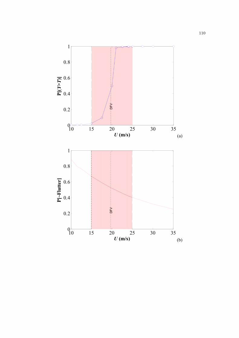
110
(a)
(b)
10 15 20 25 30 350
0.2
0.4
0.6
0.8
1
P[(Y
>T
)]
U (m/s)
DF
V
10 15 20 25 30 350
0.2
0.4
0.6
0.8
1
P[~
Flu
tter
]
U (m/s)
DF
V
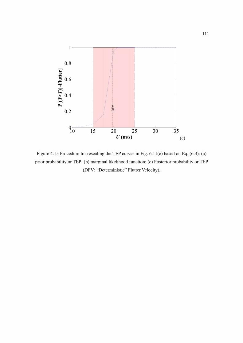
111
(c)
Figure 4.15 Procedure for rescaling the TEP curves in Fig. 6.11(c) based on Eq. (6.3): (a)
prior probability or TEP; (b) marginal likelihood function; (c) Posterior probability or TEP
(DFV: “Deterministic” Flutter Velocity).
10 15 20 25 30 350
0.2
0.4
0.6
0.8
1
P[(Y
>T
)|~F
lutt
er]
U (m/s)
DF
V
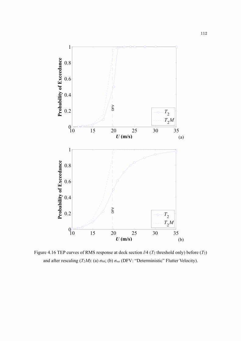
112
(a)
(b)
Figure 4.16 TEP curves of RMS response at deck section l/4 (T2 threshold only) before (T2)
and after rescaling (T2M): (a) σhh; (b) σαα (DFV: “Deterministic” Flutter Velocity).
10 15 20 25 30 350
0.2
0.4
0.6
0.8
1
Pro
babi
lity
of E
xcee
danc
e
U (m/s)
DF
VT
2
T2M
10 15 20 25 30 350
0.2
0.4
0.6
0.8
1
Pro
babi
lity
of E
xcee
danc
e
U (m/s)
DF
V
T2
T2M

113
(a)
(b)
Figure 4.17 TEP curves of RMS responses with thresholds based on the RMS
displacement, deck section at l/4 and NEU’s flutter derivatives: (a) σhh; (b) σαα.
10 15 20 25 30 350
0.2
0.4
0.6
0.8
1
Pro
bab
ilit
y of
Exc
eed
ance
U (m/s)
T1
T2
T3
T2M
10 15 20 25 30 350
0.2
0.4
0.6
0.8
1
Pro
bab
ilit
y of
Exc
eed
ance
U (m/s)
T1
T2
T3
T2M

114
(a)
(b)
1020
3040
-40-20
020
400
0.5
1
U (m/s) (deg)
Pro
bab
ility
of
Exc
eed
ance
1020
3040
-40-20
020
400
0.5
1
U (m/s) (deg)
Pro
bab
ility
of
Exc
eed
ance
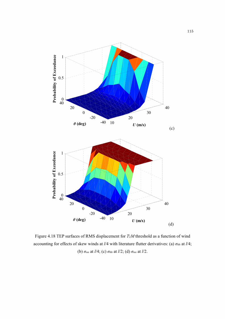
115
(c)
(d)
Figure 4.18 TEP surfaces of RMS displacement for T2M threshold as a function of wind
accounting for effects of skew winds at l/4 with literature flutter derivatives: (a) σhh at l/4;
(b) σαα at l/4; (c) σhh at l/2; (d) σαα at l/2.
1020
3040
-40-20
020
400
0.5
1
U (m/s) (deg)
Pro
bab
ility
of
Exc
eed
ance
1020
3040
-40-20
020
400
0.5
1
U (m/s) (deg)
Pro
bab
ility
of
Exc
eed
ance

116
(a)
(b)
1020
3040
-40-20
020
400
0.5
1
U (m/s) (deg)
Pro
bab
ility
of
Exc
eed
ance
1020
3040
-40-20
020
400
0.5
1
U (m/s) (deg)
Pro
bab
ility
of
Exc
eed
ance
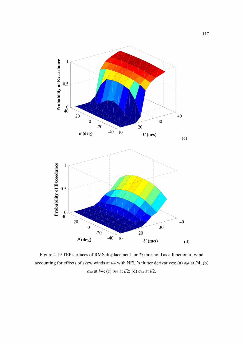
117
(c)
(d)
Figure 4.19 TEP surfaces of RMS displacement for T2 threshold as a function of wind
accounting for effects of skew winds at l/4 with NEU’s flutter derivatives: (a) σhh at l/4; (b)
σαα at l/4; (c) σhh at l/2; (d) σαα at l/2.
1020
3040
-40-20
020
400
0.5
1
U (m/s) (deg)
Pro
bab
ility
of
Exc
eed
ance
1020
3040
-40-20
020
400
0.5
1
U (m/s) (deg)
Pro
bab
ility
of
Exc
eed
ance

118
Figure 4.20 National Data Buoy Center (NOAA Station 9414290, Latitude: 37.807 N,
Longitude: 122.465 W) (Photo reproduced from NOAA, http://www.ndbc.noaa.gov/).

119
Figure 4.21 PDFs of “parent” (continuous time) mean wind velocity and annual maxima of
mean wind velocity, data from NOAA (NOAA).
0 20 40 60 80 1000
0.02
0.04
0.06
0.08
0.1
0.12
U (m/s)
PD
F
Parent wind velocityAnnual peak wind velocity
120
Chapter 5
Lifetime Cost Analysis due to Buffeting Response on a
Long-Span Bridge, accounting for Variability in Flutter
Derivatives
5.1 Introduction
This chapter discusses the estimation of lifetime cost analysis for a long-span bridge due to
wind-induced damages (i.e., monetary losses which can be associated with interventions
needed to ensure safety). In the estimation of the costs the variability in the flutter derivative
(FDs) is included. The focus of the chapter is on the buffeting bridge response.
The cost analysis employs the Monte-Carlo-based methodology for buffeting
response, described in Chapter 4. In the proposed probabilistic setting, “threshold
exceedance probability” (TEP) curves and surfaces are used to estimate the probability that
a given threshold for the variance of the response is exceeded. These probabilities are used,
together with information on the probability of the wind velocity at a given site, to predict
121
the expected value of a “lifetime monetary loss function”, derived for wind-induced
buffeting response.
The set of threshold levels, used in this chapter to derive these graphs, is different
from the ones used in Chapter 4. Thresholds are re-selected and based on both peak deck
acceleration (for user comfort) and peak dynamic displacements (e.g., for deformation of the
bridge deck or superstructure). Peak responses were directly estimated from the RMS
displacements through the gust effect factor (e.g., (Scanlan and Jones 1990a)). This choice
is dictated by the need for more realistically replicating actual damage scenarios on a large
bridge structure. The proposed model for “cost analysis” was adapted from an existing life-
cycle simulation algorithm for earthquake hazards (Wen and Kang 2001). The same truss-
type 1200m truss-type bridge model, analyzed in the previous chapters, was used in this
chapter.
5.2 Peak Estimation via RMS Response
The peak value of the dynamic displacement at any given deck section, either vertical
displacement h or torsional rotation α, can be determined by multiplying the RMS response
value by the peak effect factor (g). This factor was calculated through the equation proposed
by Davenport (Davenport 1964), which is strictly valid for a stationary random processes,
as follows:
(5.1) 0, 0
0, 0
0.577ˆ2log ,ˆ2log
e y
e y
g E g TT
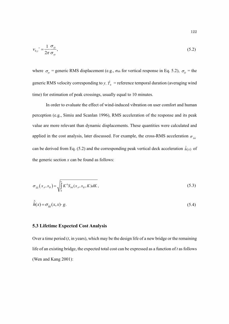
122
(5.2)
where = generic RMS displacement (e.g., σhh for vertical response in Eq. 5.2), = the
generic RMS velocity corresponding to y, = reference temporal duration (averaging wind
time) for estimation of peak crossings, usually equal to 10 minutes.
In order to evaluate the effect of wind-induced vibration on user comfort and human
perception (e.g., Simiu and Scanlan 1996), RMS acceleration of the response and its peak
value are more relevant than dynamic displacements. These quantities were calculated and
applied in the cost analysis, later discussed. For example, the cross-RMS acceleration hh
can be derived from Eq. (5.2) and the corresponding peak vertical deck acceleration of
the generic section x can be found as follows:
(5.3)
(5.4)
5.3 Lifetime Expected Cost Analysis
Over a time period (t, in years), which may be the design life of a new bridge or the remaining
life of an existing bridge, the expected total cost can be expressed as a function of t as follows
(Wen and Kang 2001):
0,
1,
2yy
yyy
yy yy
0̂T
ˆ( )h x
4
0
, ( , , ) ,A B hh A Bhhx x K S x x K dK
ˆ( ) ( , ) .hh
h x x x g
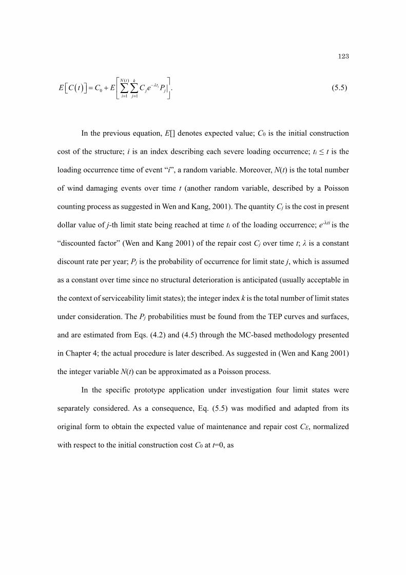
123
(5.5)
In the previous equation, E[] denotes expected value; C0 is the initial construction
cost of the structure; i is an index describing each severe loading occurrence; ti ≤ t is the
loading occurrence time of event “i”, a random variable. Moreover, N(t) is the total number
of wind damaging events over time t (another random variable, described by a Poisson
counting process as suggested in Wen and Kang, 2001). The quantity Cj is the cost in present
dollar value of j-th limit state being reached at time ti of the loading occurrence; e-λti is the
“discounted factor” (Wen and Kang 2001) of the repair cost Cj over time t; λ is a constant
discount rate per year; Pj is the probability of occurrence for limit state j, which is assumed
as a constant over time since no structural deterioration is anticipated (usually acceptable in
the context of serviceability limit states); the integer index k is the total number of limit states
under consideration. The Pj probabilities must be found from the TEP curves and surfaces,
and are estimated from Eqs. (4.2) and (4.5) through the MC-based methodology presented
in Chapter 4; the actual procedure is later described. As suggested in (Wen and Kang 2001)
the integer variable N(t) can be approximated as a Poisson process.
In the specific prototype application under investigation four limit states were
separately considered. As a consequence, Eq. (5.5) was modified and adapted from its
original form to obtain the expected value of maintenance and repair cost CE, normalized
with respect to the initial construction cost C0 at t=0, as
( )
01 1
.i
N t kt
j ji j
E C t C E C e P

124
'
( )
1 11
( )
2 210
( )0
3 31
( )
4 41
i
i
i
i
N tt
i
N tt
i
E N tt
i
N tt
i
E e P
E e PE C t C
CC
E e P
E e P
'
( )
1
( )
1
( )
1
( )
1
=1 only,User comfort
=2 only, Deformation, lower tolerance
=3 only, Deformation, higher tolerance
=4 only, Collapse
N t
i
N t
i
N t
i
N t
i
j
j
j
j
(5.6)
In Eq. (5.6) the cost, associated with each limit state, is expressed as εjC0 (j=1,2,3,4)
with εj being the ratio of this cost relative to C0. The expected value of intervention cost
normalized to the initial construction cost in Eq. (5.6), εj (j=1,2,3,4) will be discussed in
Section 5.8 along with the numerical example. In Eq. (5.6) the expected value of the cost
was found by categorizing the number of occurrences for wind events into “moderate wind
storm” (serviceability and buffeting limit states from j=1 to j=3) and “severe wind storm”
(j=4, collapse induced by the onset of flutter). This selection was dictated by the need for
separating the frequent occurrences of a moderate wind-speed storm (based on a Poisson
counting process N(t)) with extremely rare and severe events (with N’(t)<N(t)). Therefore,
the arrival rate of each Poisson Process, N(t) and N’(t), was taken as distinct.
In particular, the number of occurrences for moderate wind storms N(t) at time t was
based on a Poisson Process with an annual occurrence rate, derived from the probability of
annual wind speed maxima exceeding U=20 m/s, based on actual site winds in the proximity
of the actual bridge; this is equal to 0.94 independent of direction θ. This wind speed value
was chosen to reflect a minimum demand level, corresponding to a small but non-negligible

125
deck vibration (e.g., vertical vibrations exceeding 0.27 m or 1/30 of the deck height D). The
j=4 limit state employs a second Poisson counting process N’(t) with a much smaller
occurrence rate; the latter rate was determined as the probability of annual mean wind speed
maxima exceeding a wind speed (U) equal to the median of the critical flutter velocity
distribution for this bridge, considering variability and uncertainty in flutter derivatives, and
for wind direction orthogonal to the bridge axis (θ=0°). The median of the critical velocity
was estimated as U = 60 m/s, which leads to 0.01 as the mean occurrence rate of N’(t).
Table 5.1 shows the limit states employed in the cost analysis for the case study.
Three thresholds for limit states (T1 to T3) were used in the cost analysis under buffeting
response. The level T1, associated with limit state j=1 and maximum vertical deck
accelerations, was selected as a user comfort level based on human perception (e.g., Simiu
and Scanlan, 1996). The thresholds associated with maximum vertical dynamic
displacements was sub-categorized as T2 (limit state j=2) and T3 (limit state j=3); T2 is a more
stringent level (lower tolerance) and T3 is a less restrictive level (higher tolerance). In Table
5.1 the threshold T1 was taken as 20 milli-g of peak deck dynamic acceleration; T2 and T3
were taken as 1 m and 2 m of peak vertical deck oscillation, respectively (simulating
unacceptable deformation in the bridge deck or superstructure during serviceability). They
are all applied to buffeting response analysis and response. On the contrary, the quantity T4
was applied to the onset of flutter and collapse; and T4 was separately analyzed. The
thresholds listed in Table 5.1 were employed in the TEP analysis for vertical deck vibrations;
the same thresholds were used for peak torsional acceleration and deck rotation and
normalized with respect to B in order to be compatible with an equivalent vertical oscillation

126
of the same order of magnitude (for example with T1 being equal to 20 milli-g, T2 equal to 1
m and T3 equal to 2 m).
5.4 Description of the Structural and Aeroelastic Model
For the cost analysis a four-mode buffeting and flutter analysis of the Golden Gate Bridge
model was carried out by considering the first two vertical (v1 and v2) and torsional modes
(t1 and t2) with frequencies nv1 = 0.087 Hz and nv2 = 0.129 Hz, nt1 = 0.192 Hz and nt2 =
0.197 Hz. Simplified mode shapes were used to describe the deck and cable vibration, as
assumed in Chapters 3, 4 and in Figs. 3.5(b,d,g,h).
The TEP curves for T1 to T3 in Table 5.1 were first calculated using the model curves
based on the literature data (Jain et al. 1998 and Section 4.3.2); as described in previous
chapters the statistical properties of the coefficients of the model curves were synthetically
reproduced since no FD error analysis was available.
As a second example, TEP curves were estimated from the results from the tests
conducted at NEU, in which the eight flutter derivatives H1*,…, H4
* and A1*,…, A4
* of the
section model in Fig. 3.5 were found. The first- and second-moment properties of the
experimental errors were evaluated by repeating the measurements numerous times, as
described in Chapter 3.
For both sets of flutter derivatives the “randomization” of H1*,…, H4
* and A1*,…,
A4* was carried out by means of the model curves introduced in Chapter 3.

127
5.5 Estimation of Peak Dynamic Response during Buffeting
Peak estimation via RMS dynamic response with a zero skew wind angle is discussed in this
section. As a first implementation of the model for cost analysis, both peak dynamic
displacements and accelerations were restricted to the deck section at quarter span
(x=l/4=400 m) (i.e., cross-section at the anti-nodal point of the fundamental modes “v1” and
“t1”).
Initially, a “deterministic buffeting” analysis without considering variability in the
FDs was carried out to estimate the reference values of the peak vibration at the quarter-span
section of the deck and for verification that the oscillation magnitudes were indeed
realistically compatible and consistent with an increment of mean wind speed. An example
of peak estimation for wind orthogonal to the bridge is shown in Fig. 5.1 for both Jain’s data
and NEU’s data. For example, the comparison of peak vertical displacements is shown in
Fig. 5.1(a); vertical accelerations were calculated in terms of milli-g (mg) in Fig. 5.1(b). The
effect of the static wind loads on deck vertical displacements and rotations were also
estimated but were not incorporated in the figure due to their negligible influence in
comparison with dynamic effects. Both graphs clearly show that the peak values increase
non-linearly with increasing mean wind velocity U. Furthermore, peak vertical-response
displacements (Fig. 5.1a), using Jain’s flutter derivatives, are lower than the ones based on
flutter derivatives from NEU tests.
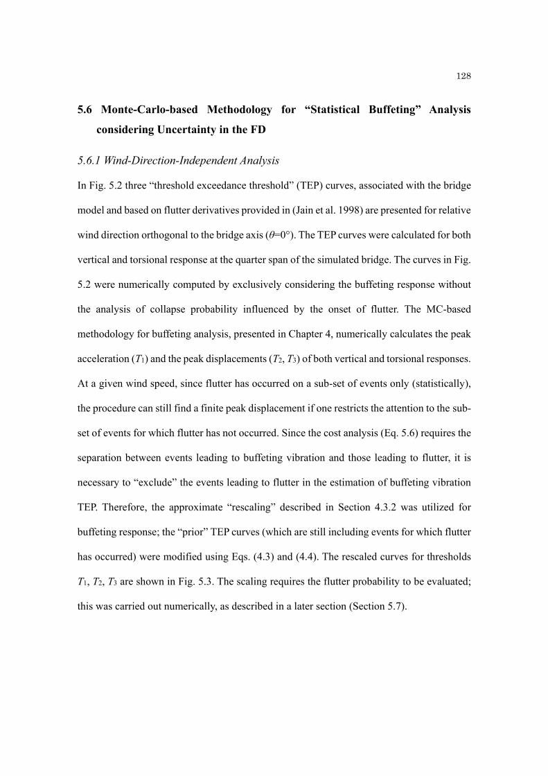
128
5.6 Monte-Carlo-based Methodology for “Statistical Buffeting” Analysis
considering Uncertainty in the FD
5.6.1 Wind-Direction-Independent Analysis
In Fig. 5.2 three “threshold exceedance threshold” (TEP) curves, associated with the bridge
model and based on flutter derivatives provided in (Jain et al. 1998) are presented for relative
wind direction orthogonal to the bridge axis (θ=0°). The TEP curves were calculated for both
vertical and torsional response at the quarter span of the simulated bridge. The curves in Fig.
5.2 were numerically computed by exclusively considering the buffeting response without
the analysis of collapse probability influenced by the onset of flutter. The MC-based
methodology for buffeting analysis, presented in Chapter 4, numerically calculates the peak
acceleration (T1) and the peak displacements (T2, T3) of both vertical and torsional responses.
At a given wind speed, since flutter has occurred on a sub-set of events only (statistically),
the procedure can still find a finite peak displacement if one restricts the attention to the sub-
set of events for which flutter has not occurred. Since the cost analysis (Eq. 5.6) requires the
separation between events leading to buffeting vibration and those leading to flutter, it is
necessary to “exclude” the events leading to flutter in the estimation of buffeting vibration
TEP. Therefore, the approximate “rescaling” described in Section 4.3.2 was utilized for
buffeting response; the “prior” TEP curves (which are still including events for which flutter
has occurred) were modified using Eqs. (4.3) and (4.4). The rescaled curves for thresholds
T1, T2, T3 are shown in Fig. 5.3. The scaling requires the flutter probability to be evaluated;
this was carried out numerically, as described in a later section (Section 5.7).

129
Figure 5.4 shows the TEP curves obtained with NEU’s experimental data, shown in
Fig. 3.5, and for a mean wind direction orthogonal to the bridge axis (θ=0°). These curves
were also based on the same threshold levels as in Table 5.1 and after rescaling (Eq. 4.3).
The comparison of TEP curves considers both Jain’s data and NEU’s data; the curves
are shown in Figs 5.5 and 5.6. The TEP curves using NEU’s data for vertical response are
shifted to the left of the graph, i.e., toward a lower wind velocity region in comparison with
Jain’s data for T1 T2 and T3. In contrast, the situation seems opposite for torsional response
since the curves using NEU’s data are shifted to the right of the graphs.
The comparison between the two curves for each threshold level in Figs. 5.5 and 5.6,
based on Jain’s FD data and NEU’s FD data, also suggests that the variability in the
aeroelastic loads plays a significant role in the input-to-output uncertainly propagation for
the analysis of the buffeting response for this bridge example. Exceedance probabilities are
crucially influenced by the flutter derivatives which are employed. A reduction in
exceedance probability is observed if the flutter derivatives from Jain’s data were used to
estimate the wind loading and deck response. This observation is valid for the vertical
dynamic deck response only and the deck section at the quarter span: in Fig. 5.5 for U=25
m/s the exceedance probability of the T2 threshold is less than 15% with Jain’s derivatives
whereas it is almost 86% for NEU’s data. In contrast, the torsional response appears to be
opposite.
5.6.2 Wind-Direction-Dependent Analysis
Figures 5.7 and 5.8 shows the TEP surfaces for vertical and torsional response, based on
flutter derivatives from Jain’s data (Fig 3.6) and corresponding to the thresholds in Table 5.1

130
(for vertical response thresholds are: T1 = 20 milli-g, T2 = 1 m and T3 = 2 m). A relative skew
wind angle, varying from θ = –40° to θ = 40°, was exclusively considered. Figures 5.9 and
5.10 show the TEP surfaces as a function of U and θ for vertical and torsional response,
based on flutter derivatives from NEU, corresponding to the same thresholds as in Table 5.1.
The analysis of all TEP surfaces, Figs. 5.7 through 5.10, confirms that the relative
skew wind angle equal to zero degrees is the most critical direction for both vertical and
torsional buffeting responses.
5.7 Flutter Analysis: Numerical Results
The flutter velocity in the absence of flutter derivative errors (i.e., “deterministic”) is equal
to 19.7 m/s for Jain’s derivatives, whereas is larger than 80.0 m/s for NEU’s data. The
“statistical” flutter velocity accounting for FD uncertainty was investigated and used to
determine the limit-state probability P4 in Eq. (5.6).
The Probability Density Function (PDF) and Cumulative Density Function (CDF) of
flutter velocity Ucr were numerically calculated from the histograms of occurrences, derived
through a MC-based sample at various skew wind angles (–40° ≤ θ ≤40°) exclusively using
NEU’s flutter derivatives; three cases (θ = 0°, 20°, and 40°) are compared and shown in Fig.
5.11. In order to increase accuracy in the Monte-Carlo estimation of low probabilities, a total
of 50,000 Monte-Carlo realizations were employed to synthetically generate the random set
of flutter derivatives for stochastic flutter analysis (Seo and Caracoglia 2011). As for the
buffeting analysis, random flutter derivatives were generated from the polynomial model
curves with random coefficients described in Section 3.6.

131
The accuracy of the Monte-Carlo estimation in relation to the number of realizations
(NMC) was also analyzed by comparing the numerical estimation of the CDF with the
“standard error measure”. The standard error can be defined as (Bucher 2009)
2 .E MCS N (5.7)
According to Bucher (2009), the variance of the CDF estimator was not derived by
repeated evaluation of the flutter probability (PUcr) but was approximately assessed along
the Ucr axis from the curve corresponding to case with θ=0° in Fig. 5.11(b) as
.U crcr
P U MCP N (5.8)
Figure 5.12 was also used for “guidance” to provide indications for sufficient or
insufficient resolution of the stochastic flutter analysis, since it compares the absolute
differences between any two contiguous numerical flutter CDFs at various θ (i.e., the curves
shown in Fig. 5.11) to the standard error (Eq. 5.6). For example, the blue dotted line in Fig.
5.12 is the absolute difference between the two cases for mean wind incident angles θ=0°
and θ=20°; this difference is greater than the standard error (red solid line) when flutter
velocity is approximately less than 85 m/s. The black dashed-dotted line is the absolute
difference between the two cases with θ=20° and θ=40°; this quantity is greater than the
standard error (red solid line) when Ucr ≤ 90 m/s. The interval of Ucr where the relative

132
difference between any two scenarios (absolute variations due to change in skew wind angle
θ) is greater than the standard error can be used as a “confidence region” with acceptable
resolution.
As a result of the comparisons in Fig. 5.12, it was suggested that an “acceptance
region” in the MC-based methodology for stochastic flutter speed with skew wind angle can
be approximately found for mean wind speed less than 80 m/s; this velocity is usually lower
that the upper limits used to estimate the TEP curves and surfaces presented in this chapter.
The probability of the onset of flutter (PUcr) also coincides with the limit-state
probability P4 in Eq. (5.6). As a result of numerical flutter analysis, the limit-state probability
P4 was numerically found as 0.0029 for the case using Jain’s FD data and 0.0964 with NEU’s
FD data. The flutter probabilities P4 for both cases (i.e., using Jain’s FDs and NEU’s FDs)
will not be considered in the cost analysis.
5.8 Lifetime Expected Intervention Cost Analysis - Numerical Results
In this section, an example of expected lifetime cost analysis is described. NEU’s FD data
was exclusively used for buffeting simulations considering the uncertainty in the flutter
derivatives.
5.8.1 Estimation of the Limit-State Probabilities Pj from TEP Analysis
Table 5.2 shows the probabilities of each limit state (Pj) based on the buffeting intervention
thresholds described in Table 5.1 for both the case with considering the variability in the FD
and the case in the absence of the variability. As outlined earlier, the threshold level T1 for
user comfort and two levels for deck deformation were investigated: T2 a more conservative

133
intervention threshold level and T3 a less restrictive level. However, inspection revealed that
the limit state probabilities P2 and P3 for torsional response are zero values for 0<U<80 m/s
when variability in FD is neglected (i.e., for “deterministic buffeting”). This remark confirms
that “deterministic buffeting” analysis underestimates the loss function significantly without
further investigation. Therefore, the results of the TEP analysis for vertical deck response
were exclusively used in the cost analysis.
As described in previous sections and in Table 5.2 the threshold T1 used in the cost
analysis corresponds to peak deck dynamic acceleration (comfort of users); T2 and T3
correspond to the peak vertical deck oscillation requiring intervention for serviceability.
These three thresholds (i.e., T1, T2 and T3) are estimated from dynamic buffeting analysis.
The probabilities in Table 5.2 were computed from the TEP surfaces in Fig. 5.9
through Fig. 5.10. As originally introduced in Eq. (4.5), if the TEP surface is derived from
the equation below
FTj(U,θ) = P[Y>Tj|U = u,Θ = θ], (5.9)
the probability for limit states j=1,2,3 is
Pj = ∫∫FTj(U,θ)fU(U)fθ(θ)dθdU. (5.10)
In Eq. (5.10) the probability density functions of the wind speed fU(U) and mean
wind direction fθ(θ) were obtained from the “raw” wind data, assuming U and θ as
independent random variables, recorded at the meteorological station close to the benchmark

134
bridge, as described in Section 4.5. The histogram of annual 10-minute averaged wind speed
maxima shown in Fig. 4.21 was derived from the NOAA annual wind speed maxima over a
16-year period (1996-2011) and was employed to evaluate fU(U). A detailed description of
the station and data resources can also be found in (Seo and Caracoglia 2012).
Derivation of the probability density functions of the annual wind speed maxima (fU)
and mean skew wind angle (fθ) enabled the estimation of Pj (j=1,2,3) in Eq. (5.10) after TEP
analysis (Section 5.5).
5.8.2 Expected Intervention Cost - Description of the Simulations
Probability mass function (PMF) was utilized to investigate how the cost varies with a
random arrival time of each wind event (ti and ti’ in Eq. 5.6). The arrival time of the events
was modeled as a uniform random variable between 0 and t (or 0 and t’) with the counting
of the total number of Poisson’s events, N(t) or N’(t). Monte-Carlo sampling was employed
to estimate the PMF of the relative maintenance and repair cost, (C(t)-C0)/C0, using 500
repeated Monte-Carlo realizations and five percent discount rate/year (λ). Intervention
criteria can be found in Table 5.1 (Tj, j=1,2,3,4); a time projection of 80 years was initially
used; probabilities of exceeding the limit states were taken from the Pj values in Table 5.2
(j=1,2,3). The ratio of this cost relative to construction cost C0 was chosen to be 20% for all
intervention levels ε1, ε2, ε3. The results of the cost analysis are summarized in Figs. 5.13 and
5.14. These figures were compiled based on two different intervention criteria: Fig. 5.13 for
user comfort (i.e., P1), and Fig. 5.14 due to deformation in the deck (i.e., P2 or P3). Five
markers (black +, blue ◊, cyan ○, magenta □, and green Δ) and one red solid line are shown
in the stem plots (Fig. 5.13). Each point on the stem plots represents a probability range: +
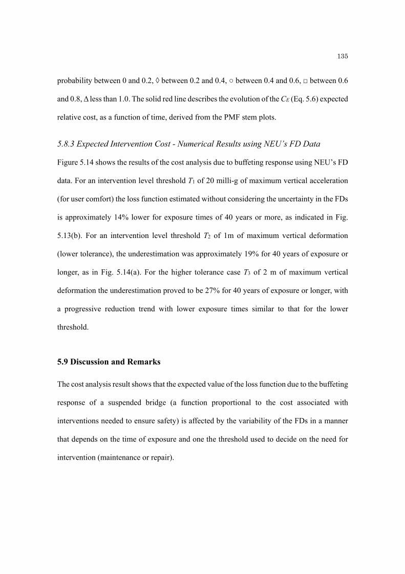
135
probability between 0 and 0.2, ◊ between 0.2 and 0.4, ○ between 0.4 and 0.6, □ between 0.6
and 0.8, Δ less than 1.0. The solid red line describes the evolution of the CE (Eq. 5.6) expected
relative cost, as a function of time, derived from the PMF stem plots.
5.8.3 Expected Intervention Cost - Numerical Results using NEU’s FD Data
Figure 5.14 shows the results of the cost analysis due to buffeting response using NEU’s FD
data. For an intervention level threshold T1 of 20 milli-g of maximum vertical acceleration
(for user comfort) the loss function estimated without considering the uncertainty in the FDs
is approximately 14% lower for exposure times of 40 years or more, as indicated in Fig.
5.13(b). For an intervention level threshold T2 of 1m of maximum vertical deformation
(lower tolerance), the underestimation was approximately 19% for 40 years of exposure or
longer, as in Fig. 5.14(a). For the higher tolerance case T3 of 2 m of maximum vertical
deformation the underestimation proved to be 27% for 40 years of exposure or longer, with
a progressive reduction trend with lower exposure times similar to that for the lower
threshold.
5.9 Discussion and Remarks
The cost analysis result shows that the expected value of the loss function due to the buffeting
response of a suspended bridge (a function proportional to the cost associated with
interventions needed to ensure safety) is affected by the variability of the FDs in a manner
that depends on the time of exposure and one the threshold used to decide on the need for
intervention (maintenance or repair).
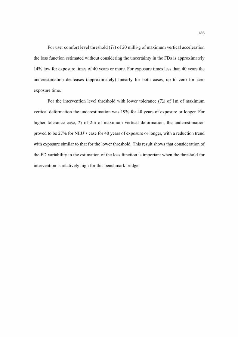
136
For user comfort level threshold (T1) of 20 milli-g of maximum vertical acceleration
the loss function estimated without considering the uncertainty in the FDs is approximately
14% low for exposure times of 40 years or more. For exposure times less than 40 years the
underestimation decreases (approximately) linearly for both cases, up to zero for zero
exposure time.
For the intervention level threshold with lower tolerance (T2) of 1m of maximum
vertical deformation the underestimation was 19% for 40 years of exposure or longer. For
higher tolerance case, T3 of 2m of maximum vertical deformation, the underestimation
proved to be 27% for NEU’s case for 40 years of exposure or longer, with a reduction trend
with exposure similar to that for the lower threshold. This result shows that consideration of
the FD variability in the estimation of the loss function is important when the threshold for
intervention is relatively high for this benchmark bridge.

137
Table 5.1 Structural performance thresholds for vertical deck response (Tj).
Table 5.2 Probabilities of each damage state (Pj) due to buffeting response based on the
structural performance thresholds (T = Tj) using NEU’s FD data.
Flutter ThresholdHuman comfort
(T 1, peak acc.)
Lower ToleranceDeformation
(T 2, peak disp.)
Higher ToleranceDeformation
(T 3 peak disp.)
Instability
(T 4, collapse)
20 milli-g 1 m 2 m N.A.
Buffeting Thresholds (deck)
P 1 P 2 P 3
Without variability in FD 3.48E-03 3.20E-03 2.62E-03
With variability in FD 4.04E-03 3.94E-03 3.56E-03
Without variability in FD 5.96E-04 0.00E+00 0.00E+00
With variability in FD 3.58E-03 3.04E-03 2.70E-03
Probabilities of Damage State, P [Y > T ]
TorsionalResponse
VerticalResponse
Using NEU's FD Data
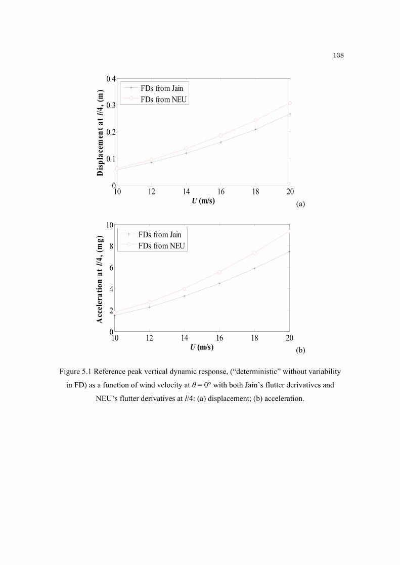
138
(a)
(b)
Figure 5.1 Reference peak vertical dynamic response, (“deterministic” without variability
in FD) as a function of wind velocity at θ = 0° with both Jain’s flutter derivatives and
NEU’s flutter derivatives at l/4: (a) displacement; (b) acceleration.
10 12 14 16 18 200
0.1
0.2
0.3
0.4
U (m/s)
Dis
pla
cem
ent
at l
/4, (
m)
FDs from JainFDs from NEU
10 12 14 16 18 200
2
4
6
8
10
U (m/s)
Acc
eler
atio
n a
t l/4
, (m
g)
FDs from JainFDs from NEU
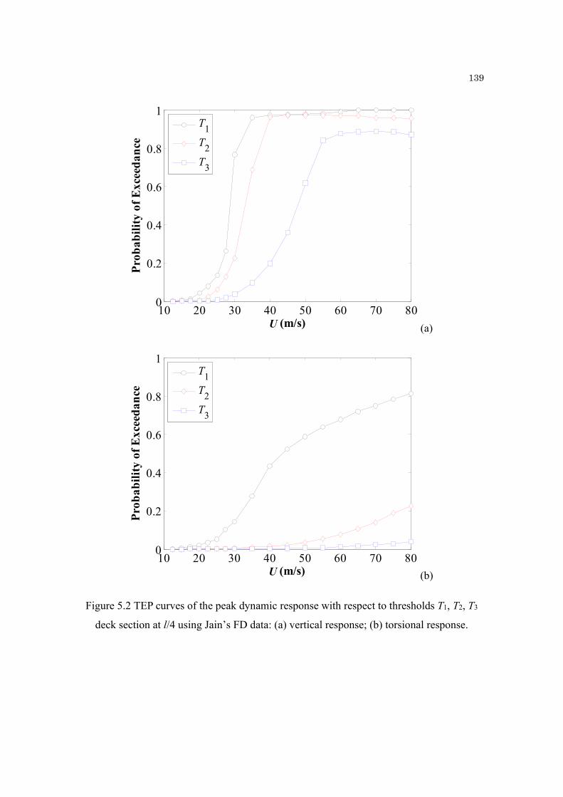
139
(a)
(b)
Figure 5.2 TEP curves of the peak dynamic response with respect to thresholds T1, T2, T3
deck section at l/4 using Jain’s FD data: (a) vertical response; (b) torsional response.
10 20 30 40 50 60 70 800
0.2
0.4
0.6
0.8
1
Pro
bab
ilit
y of
Exc
eed
ance
U (m/s)
T1
T2
T3
10 20 30 40 50 60 70 800
0.2
0.4
0.6
0.8
1
Pro
bab
ilit
y of
Exc
eed
ance
U (m/s)
T1
T2
T3

140
(a)
(b)
Figure 5.3 Recaled TEP curves (modified by Eq. 4.3) of the peak dynamic response with
respect to thresholds T1, T2, T3 deck section at l/4 using Jain’s FD data: (a) vertical
response; (b) torsional response.
10 20 30 40 50 60 70 800
0.2
0.4
0.6
0.8
1
Pro
bab
ilit
y of
Exc
eed
ance
U (m/s)
T1
T2
T3
10 20 30 40 50 60 70 800
0.2
0.4
0.6
0.8
1
Pro
bab
ilit
y of
Exc
eed
ance
U (m/s)
T1
T2
T3

141
(a)
(b)
Figure 5.4 Rescale TEP curves (modified by Eq. 4.3) of the peak dynamic response with
respect to thresholds T1, T2, T3 deck section at l/4 using NEU’s FD data: (a) vertical
response; (b) torsional esponse.
10 20 30 40 50 60 70 800
0.2
0.4
0.6
0.8
1
Pro
bab
ilit
y of
Exc
eed
ance
U (m/s)
T1
T2
T3
10 20 30 40 50 60 70 800
0.2
0.4
0.6
0.8
1
Pro
bab
ilit
y of
Exc
eed
ance
U (m/s)
T1
T2
T3

142
(a)
(b)
10 20 30 40 50 60 70 800
0.2
0.4
0.6
0.8
1
Pro
bab
ilit
y of
Exc
eed
ance
U (m/s)
T1 (NEU)
T1 (Jain)
10 20 30 40 50 60 70 800
0.2
0.4
0.6
0.8
1
Pro
bab
ilit
y of
Exc
eed
ance
U (m/s)
T2 (NEU)
T2 (Jain)

143
(c)
Figure 5.5 A comparison between two sets of curves for vertical response based on NEU’s
FD data (continuous lines) and Jain’s FD data (dotted lines): (a) T1=20 milli-g; (b) T2=1m;
(c) T3=2m.
10 20 30 40 50 60 70 800
0.2
0.4
0.6
0.8
1
Pro
bab
ilit
y of
Exc
eed
ance
U (m/s)
T3 (NEU)
T3 (Jain)

144
(a)
(b)
10 20 30 40 50 60 70 800
0.2
0.4
0.6
0.8
1
Pro
bab
ilit
y of
Exc
eed
ance
U (m/s)
T1 (NEU)
T1 (Jain)
10 20 30 40 50 60 70 800
0.2
0.4
0.6
0.8
1
Pro
bab
ilit
y of
Exc
eed
ance
U (m/s)
T2 (NEU)
T2 (Jain)

145
(c)
Figure 5.6 A comparison between two sets of curves for torsional response based on
NEU’s FD data (continuous lines) and Jain’s FD data (dotted lines): (a) T1=20 milli-g; (b)
T2=1m; (c) T3=2m.
10 20 30 40 50 60 70 800
0.2
0.4
0.6
0.8
1
Pro
bab
ilit
y of
Exc
eed
ance
U (m/s)
T3 (NEU)
T3 (Jain)

146
(a)
(b)
2040
6080
-40-20
020
400
0.5
1
U (m/s) (deg)
Pro
bab
ilit
y of
Exc
eed
ance
2040
6080
-40-20
020
400
0.5
1
U (m/s) (deg)
Pro
bab
ilit
y of
Exc
eed
ance
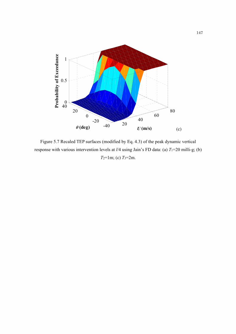
147
(c)
Figure 5.7 Recaled TEP surfaces (modified by Eq. 4.3) of the peak dynamic vertical
response with various intervention levels at l/4 using Jain’s FD data: (a) T1=20 milli-g; (b)
T2=1m; (c) T3=2m.
2040
6080
-40-20
020
400
0.5
1
U (m/s) (deg)
Pro
bab
ilit
y of
Exc
eed
ance
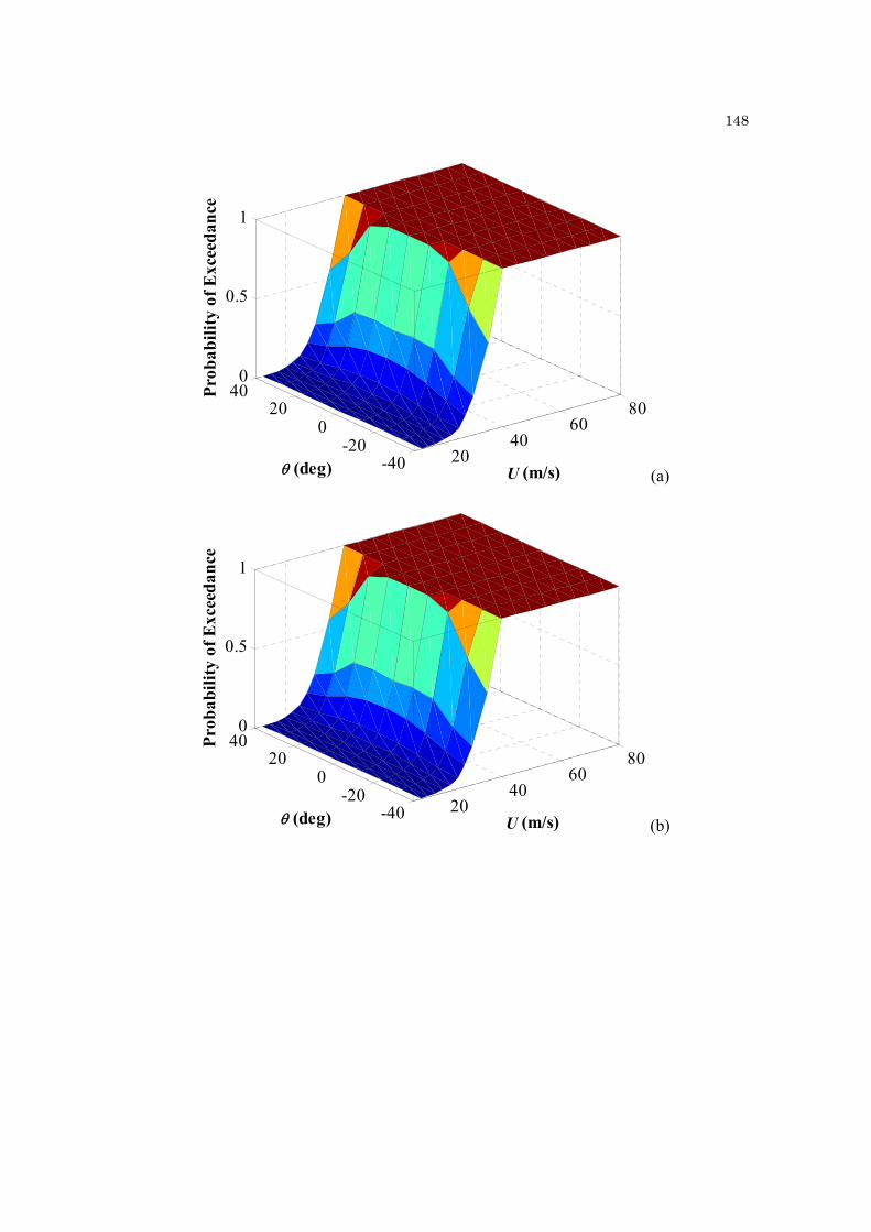
148
(a)
(b)
2040
6080
-40-20
020
400
0.5
1
U (m/s) (deg)
Pro
bab
ilit
y of
Exc
eed
ance
2040
6080
-40-20
020
400
0.5
1
U (m/s) (deg)
Pro
bab
ilit
y of
Exc
eed
ance
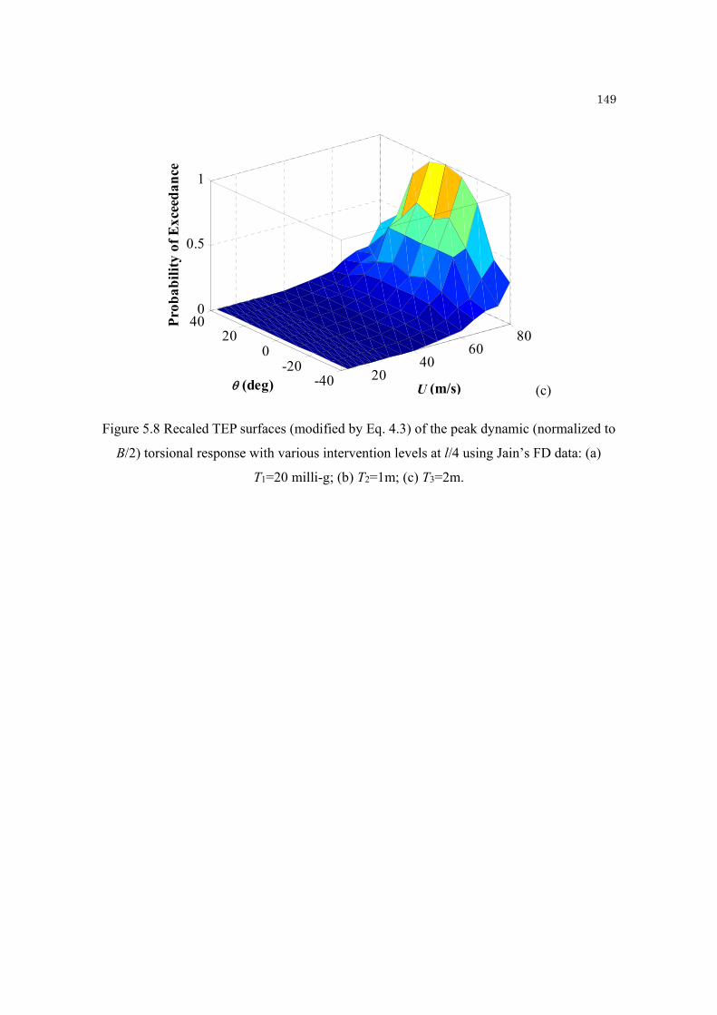
149
(c)
Figure 5.8 Recaled TEP surfaces (modified by Eq. 4.3) of the peak dynamic (normalized to
B/2) torsional response with various intervention levels at l/4 using Jain’s FD data: (a)
T1=20 milli-g; (b) T2=1m; (c) T3=2m.
2040
6080
-40-20
020
400
0.5
1
U (m/s) (deg)
Pro
bab
ilit
y of
Exc
eed
ance

150
(a)
(b)
2040
6080
-40-20
020
400
0.5
1
U (m/s) (deg)
Pro
bab
ilit
y of
Exc
eed
ance
2040
6080
-40-20
020
400
0.5
1
U (m/s) (deg)
Pro
bab
ilit
y of
Exc
eed
ance

151
(c)
Figure 5.9 Recaled TEP surfaces (modified by Eq. 4.3) of the peak dynamic vertical
response with various intervention levels at l/4 using NEU’s FD data: (a) T1=20 milli-g; (b)
T2=1m; (c) T3=2m.
2040
6080
-40-20
020
400
0.5
1
U (m/s) (deg)
Pro
bab
ilit
y of
Exc
eed
ance
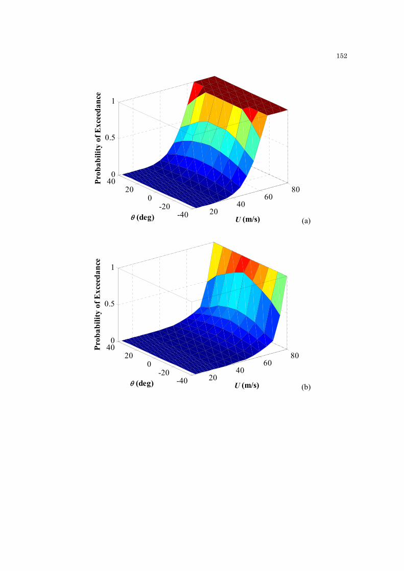
152
(a)
(b)
2040
6080
-40-20
020
400
0.5
1
U (m/s) (deg)
Pro
bab
ilit
y of
Exc
eed
ance
2040
6080
-40-20
020
400
0.5
1
U (m/s) (deg)
Pro
bab
ilit
y of
Exc
eed
ance
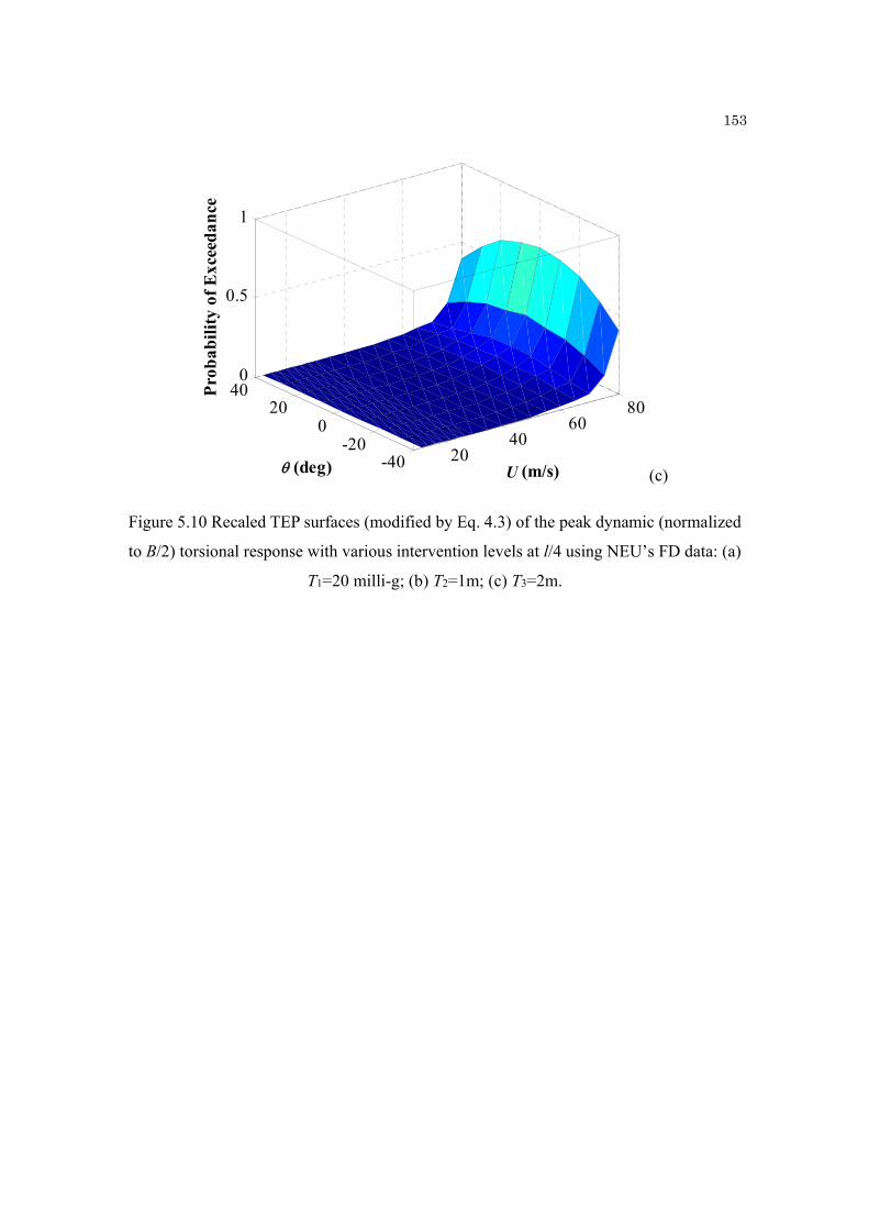
153
(c)
Figure 5.10 Recaled TEP surfaces (modified by Eq. 4.3) of the peak dynamic (normalized
to B/2) torsional response with various intervention levels at l/4 using NEU’s FD data: (a)
T1=20 milli-g; (b) T2=1m; (c) T3=2m.
2040
6080
-40-20
020
400
0.5
1
U (m/s) (deg)
Pro
bab
ilit
y of
Exc
eed
ance
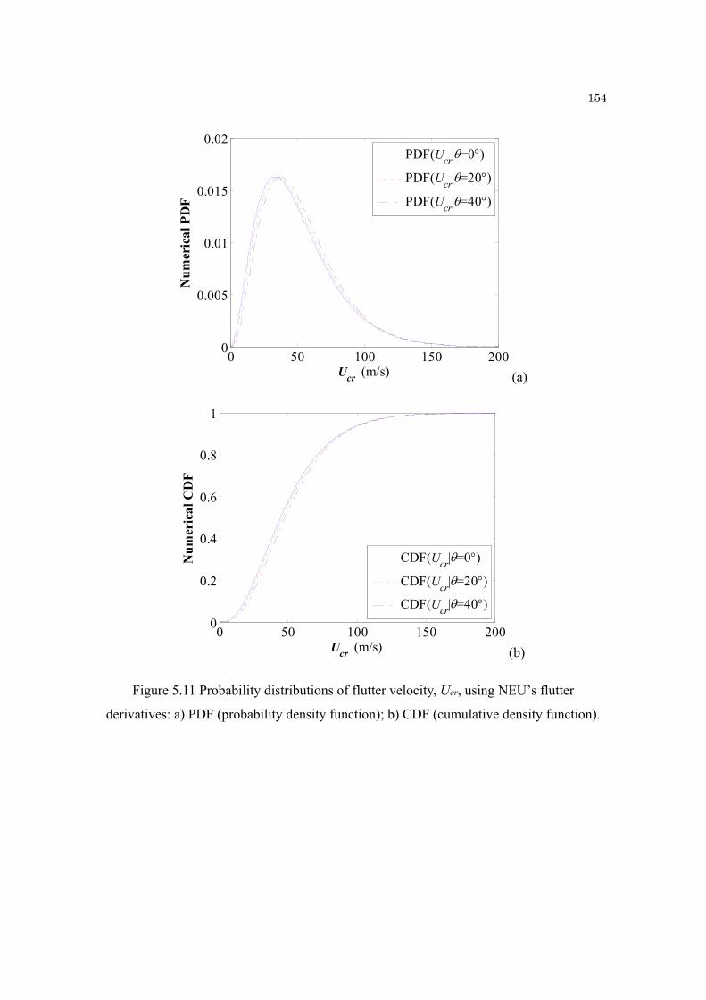
154
(a)
(b)
Figure 5.11 Probability distributions of flutter velocity, Ucr, using NEU’s flutter
derivatives: a) PDF (probability density function); b) CDF (cumulative density function).
0 50 100 150 2000
0.005
0.01
0.015
0.02
Ucr (m/s)
Nu
mer
ical
PD
F
PDF(Ucr|=0)
PDF(Ucr|=20)
PDF(Ucr|=40)
0 50 100 150 2000
0.2
0.4
0.6
0.8
1
Ucr (m/s)
Nu
mer
ical
CD
F
CDF(Ucr|=0)
CDF(Ucr|=20)
CDF(Ucr|=40)

155
Figure 5.12 Resolution of the Monte-Carlo-based flutter procedure vs. standard error.
0 50 100 150 2000
0.02
0.04
0.06
0.08
Ucr (m/s)
Res
olu
tion
CDF(Ucr|=0) - CDF(Ucr|=20)
CDF(Ucr|=20) - CDF(Ucr|=40)
Standard error

156
(a)
(b)
Figure 5.13 Intervention costs normalized to the initial construction cost for user comfort
level threshold T1=20 milli-g over time based on NEU’s FD data :
(a) 3D PMF (probability mass function stem plot); (b) 2D expected normalized cost, -
discount rate/year λ=0.05.
0
0.2
0.4
020406080
0
0.2
0.4
0.6
0.8
1
Time (yrs)Relative Cost
PM
F
0 20 40 60 800
0.02
0.04
0.06
0.08
0.1
Time (yrs)
Exp
ecte
d N
orm
aliz
ed C
ost,
CE
With Variability in FDWithout Variability in FD
0 0EC E C t C C
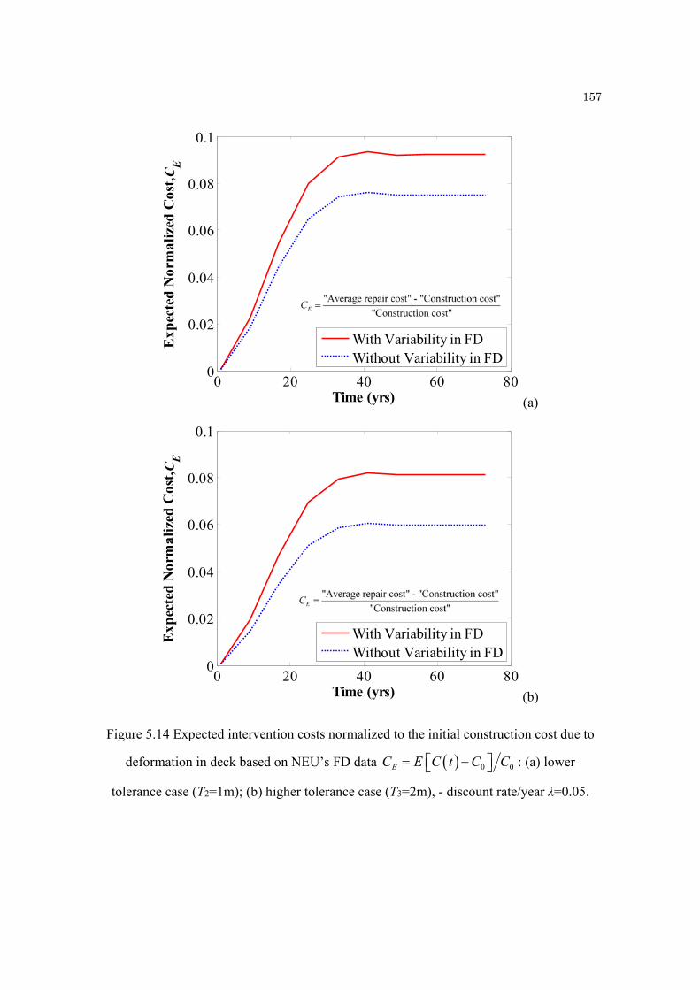
157
(a)
(b)
Figure 5.14 Expected intervention costs normalized to the initial construction cost due to
deformation in deck based on NEU’s FD data : (a) lower
tolerance case (T2=1m); (b) higher tolerance case (T3=2m), - discount rate/year λ=0.05.
0 20 40 60 800
0.02
0.04
0.06
0.08
0.1
Time (yrs)
Exp
ecte
d N
orm
aliz
ed C
ost,
CE
With Variability in FDWithout Variability in FD
0 20 40 60 800
0.02
0.04
0.06
0.08
0.1
Time (yrs)
Exp
ecte
d N
orm
aliz
ed C
ost,
CE
With Variability in FDWithout Variability in FD
0 0EC E C t C C

158
Chapter 6
Summary and Conclusions
6.1 Summary
The primary intent of the research, described in this dissertation, was to implement a
methodology for analyzing the buffeting response of cable-supported bridges, including
uncertainty in the aeroelastic input (flutter derivatives). Flutter derivatives are the most
important part of wind loading and are estimated in a wind tunnel experiment. A second
order polynomial model for the flutter derivatives was used in the research and labeled as
“model curve”.
A general discussion on the state of the art regarding the general introduction of
wind-induced phenomena of long-span bridges is carried out in Chapter 1. Also the
motivation of this research is presented. Fast and efficient integration procedures of the wind
loading acting over the deck span are also necessary for structural performance.
Chapter 2 summarizes the background theory of wind-induced response of long-span
bridges and reviews the fundamental aspects of aerodynamics and aeroelasticity of long-
span suspended bridge decks. The general approach for flutter instability and buffeting

159
response is discussed in this chapter. The effect of wind directionality on the bridge deck
response is also presented.
Chapter 3 describes the experimental setup, measurements and experimental results,
used in this research. This chapter also describes the development of a “model curve” for
representation of the behavior of flutter derivatives as a function of reduced wind velocity.
Flutter derivatives were measured in the wind tunnel at Northeastern University.
Chapter 4 discusses the buffeting analysis of long-span bridges including uncertainty
in the FD. In the first part of this chapter, “deterministic buffeting” analysis is discussed
using the model curve that the result is the value of the RMS dynamic response at a given
wind speed as the standard approach. In the second part of this chapter, “statistical buffeting”
analysis is discussed, which includes uncertainty in the FDs; the coefficients of the model
curve are treated as random variables, whose probability distribution is conditional on
reduced wind speed. The “statistical buffeting” response was evaluated by adopting the
concept of “fragility”; this was also employed in the calculation of the exceedance
probability of pre-selected vibration thresholds, conditional on mean wind speed and
direction at the deck level. Threshold exceedance probability curves and surfaces, associated
with RMS dynamic buffeting response, were numerically derived.
Finally, the expected value of the loss function due to the buffeting response of a
1200-meter suspension bridge is evaluated by considering the uncertainty in the FDs.

160
6.2 Conclusions
The findings of this research can be summarized as follows:
Regarding Performance
It is shown that the expected value of the loss function due to the buffeting response
of a suspended bridge (a function proportional to the cost associated with
interventions needed to ensure safety) is affected by the variability of the FDs in a
manner that depends on the time of exposure and one the threshold used to decide on
the need for intervention.
For an intervention level threshold of 1m of maximum vertical deformation the loss
function estimated without considering the uncertainty in the FDs is approximately
19% low for exposure times of 40 years or more. For exposure times less than 40
years the underestimation decreases (approximately) linearly, up to zero for zero
exposure time.
For an intervention level threshold of 2m of maximum vertical deformation (higher
tolerance in allowing the bridge to operate) the underestimation proved to be 27%
for 40 years of exposure or longer, with a reduction trend with exposure similar to
that for the lower threshold. This result shows that consideration of the FD variability
in the estimation of the loss function is important when the threshold for intervention
is relatively high.
161
On Computational Issues
It is shown that the RMS buffeting response of a long-span cable supported bridge
can be estimated (with sufficient accuracy to be practically useful) using a second
order polynomial description of the flutter derivatives (FDs). The uncertainty in these
derivatives in the model is captured by specifying the coefficients of the polynomial
as a vector of random variables having a specified mean and covariance (the values
of these properties used in the numerical analyses were obtained experimentally).
It is found that there is a significant computational advantage in using Monte Carlo
methods for calculating a double integral that arises on the estimating of the
generalized buffeting loading used in a multi-mode buffeting analysis. The
computational time is approximately one order of magnitude smaller than that of
using a standard integration algorithm (repeated trapezoidal rule).
It is found that the polynomial description of the FD can also be used with
computational advantages to estimate the onset of flutter.
6.3 Recommendations for Future Research
Expand the treatment of the uncertainties to include structural properties and wind
directionality.
More detailed investigation of Quasi-Monte-Carlo methods should be taken,
especially for calculating the double integral in the analysis of multi-variable
“random domains”.

162
More detailed investigation in the estimation of the expected value of the loss
function due to the buffeting response of a suspended, affected by the variability of
the FDs, should be taken.
Account for lateral dynamic bridge response in the buffeting analysis.
Include chord-wise admittance effects in the formulation of the buffeting loading.
Even though the use of chord-wise admittance can lead to a reduction of magnitude
in the buffeting loads, this effect should be included in the future.
6.4 Outcome of the PhD Studies: List of Deliverables
As of February 2013, the work, described in this dissertation, has been published or is in the
process of being published in a series of journal articles (three) and conference proceedings
(four). A description of these items is provided below for completeness.
6.4.1 Journal Publications (Published/under review)
A. Seo, D.-W. and Caracoglia, L., “Estimating Life-Cycle Monetary Losses due to Wind
Hazards: Fragility Analysis of Long-Span Bridges,” Engineering Structures, Submitted
for review, 2012.
B. Seo, D.-W. and Caracoglia, L., “Statistical Buffeting Response of Long-Span Bridges
Influenced by Errors in Aeroelastic Loading Estimation,” Journal of Wind Engineering
and Industrial Aerodynamics, Vol. 104-106, 2012, pp. 129-140. Note: The paper was
selected for potential publications in a special issue of the journal, as an extended
version of ICWE-13 Conference paper.
C. Seo, D.-W. and Caracoglia, L., “Estimation of Torsional-flutter Probability in Flexible
Bridges Considering Randomness in Flutter Derivatives,” Engineering Structures, Vol.
33, No. 8, 2011, pp. 2284–2296.

163
6.4.2 Other Journal Publications (not related to the main topic of this Dissertation)
D. Seo, D.-W. and Caracoglia, L., “Derivation of Equivalent Gust Effect Factors for Wind
Loading on Low-Rise Buildings through Database-Assisted-Design Approach,”
Engineering Structures, Vol. 32, No. 1, 2010, pp. 328-336.
6.4.3 Full Papers in Conference Proceedings
E. Seo, D.-W. and Caracoglia, L., “A Numerical Algorithm for Predicting Life-Cycle
Maintenance Costs for Slender Bridges under Wind Hazards,” Proceedings of the 3rd
Workshop of the American Association for Wind Engineering (AAWE), Hyannis,
Massachusetts, August 12-14, 2012, CD-ROM.
F. Seo, D.-W. and Caracoglia, L., “Monte-Carlo Methods for Estimating the Buffeting
Response of a Bridge Contaminated by Flutter-Derivative Errors,” Proceedings of 13th
International Conference on Wind Engineering (ICWE-13), Amsterdam, NL, July 10-
15, 2011, paper No. 214, CD-ROM.
G. Seo, D.-W. and Caracoglia, L., “Flutter Velocity Estimation using Experimentally-
Derived (Co)-Variances of Aeroelastic Coefficients,” Proceedings of the International
Conference of the Engineering Mechanics Institute (EMI2011), American Society of
Civil Engineers, Northeastern University, Boston, Massachusetts, USA, June 02-04,
2011, CD-ROM (full paper). Note: The paper was selected among the finalists for the
Probabilistic Methods Student Paper Award.
H. Seo, D.-W. and Caracoglia, L., “Quasi- and Monte-Carlo-Based Methods for Statistical
Buffeting Analysis of Long-Span Bridges under the Effects of Turbulent Wind,”
Proceedings of the 2nd Workshop of the American Association for Wind Engineering
(AAWE), Marco Island, Florida, August 18-20, 2010.
6.4.4 Other Papers Published as Conference Proceedings (not related to the main
topic of the Dissertation)
I. Seo, D.-W., Moghim, F., and Bernal, D., “Normalization of Complex Modes from Mass
Perturbations,” Proceeding of A Conference and Exposition on Structural Dynamics
164
(IMAC XXIX), Society for Experimental Mechanics, Jacksonville, FL, January 04-07,
2011, PAPER No. 41.
6.4.5 Poster Presentations
J. Seo, D.-W. and Caracoglia, L., “A Life-Cycle Cost Analysis for Structural Maintenance
of Flexible Bridges under Wind Hazards,” 2012 NSF-CMMI Engineering Research and
Innovation Conference, Boston, Massachusetts, USA, July 9–12 2012 (student poster
presentation).
K. Seo, D.-W. and Caracoglia L., “A Life-Cycle Cost Model for Structural Maintenance of
Long-Span Bridges Under Wind Hazards,” NU Research Exposition 2012, Boston,
Massachusetts, USA, April 6, 20112, Research poster No. 67.
L. Seo, D.-W. and Caracoglia, L., “Statistical Buffeting Simulations of Long-Span Bridge
Response under Wind Hazards: Fragility Curves and Surfaces,” Second US-Japan Mini
Workshop on Structural Dynamics and Monitoring of Bridges and Flexible Structures
against Wind Hazards, Boston, Massachusetts, USA, November 12-14, 2011.
M. Seo, D.-W. and Caracoglia L., “Statistical Buffeting Simulations of Long-span Bridge
Response under Wind Hazards: Recent Case Studies,” NU Research Exposition 2011,
Boston, Massachusetts, USA, April 6, 2011, No. 1968.
N. Seo, D.-W. and Caracoglia L., “Estimation of Torsional Bridge Flutter Collapse by
Numerical Statistical Methods,” NU Research Exposition 2010, Boston, Massachusetts,
USA, March 24, 2010, No. 1410. O. Seo, D.-W. and Caracoglia L., “Assessment of Gust Effect Factors for Wind Loading on
Low-rise Buildings through Database-Assisted-Design Method and Current Structural
Design Standards,” NU Research Exposition 2009, Boston, Massachusetts, USA,
March 26, 2009, No. 1294.

165
References
Barlow, J. B., Rae, W. H., and Pope, A. (1999). Low-speed wind tunnel testing (third edition),
John Wiley and sons, New York, New York, USA.
Bartoli, G., Contri, S., Mannini, C., and Righi, M. (2009). "Toward an Improvement in the
Identification of Bridge Deck Flutter Derivatives." Journal of Engineering
Mechanics, 135(8), 771-785.
Bashor, R., and Kareem, A. (2007). "Probabilistic performance evaluation of buildings: An
occupant comfort perspective." 12th International Conference on Wind Engineering
(12-ICWE), Cairns, Australia, July 1-6, 2007, 1335-1342.
Bienkiewicz, B. (1987). "Wind-tunnel study of effects of geometry modification on
aerodynamics of a cable-stayed bridge deck." Journal of Wind Engineering and
Industrial Aerodynamics, 26(3), 325-339.
Brito, R. (2008). "Extraction of aeroelastic coefficients for bridge decks from small-scale
wind tunnel tests," Northeastern Unviersity, Boston.
Brito, R., and Caracoglia, L. (2009). "Extraction of flutter derivatives from small scale wind
tunnel experiments." 11th Americas Conference on Wind Engineering, American
Association for Wind Engineering (AAWE), San Juan, Puerto Rico, CD-Rom.
Bucher, C. (2009). Computational analysis of randomness in structural mechanics, Taylor
Francis Group, London, UK.
Caracoglia, L. (2008a). "Influence of uncertainty in selected aerodynamic and structural
parameters on the buffeting response of long-span bridges." Journal of Wind
Engineering and Industrial Aerodynamics, 96(3), 327-344.
Caracoglia, L. (2008b). "Recent investigations on long-span bridge aeroelasticity in the
presence of turbulence fields with uncertain span-wise correlation." Sixth
International Colloquium on Bluff Bodies Aerodynamics & Applications (BBAA VI),
Polytechnic University of Milan, Milan, Italy, ISBN 88-901916-3-5, 152-155.

166
Caracoglia, L. (2011). "Simulation of linear and non-linear propagation effects of a random
turbulence field on bridge flutter instability." Journal of Wind Engineering and
Industrial Aerodynamics, 99(9), 945-954.
Caracoglia, L., and Jones, N. P. (2003). "Time domain vs. frequency domain characterization
of aeroelastic forces for bridge deck sections." Journal of Wind Engineering and
Industrial Aerodynamics, 91(3), 371-402.
Caracoglia, L., and Velazquez, A. (2007). "Sensitivity of long-span bridge buffeting response
predictions to uncertainty in the definition of selected flutter derivatives." 12th
International Conference on Wind Engineering (12-ICWE), Cairns, Australia, July
1-6, 2007, 135-142.
Chowdhury, A. G., and Sarkar, P. P. (2003). "A new technique for identification of eighteen
flutter derivatives using a three-degree-of-freedom section model." Engineering
Structures, 25(12), 1763–1772.
Davenport, A. G. (1962). "Buffeting of a suspension bridge by storm winds." Journal of
Structural Division, ASCE, 88(ST3), 233-264.
Davenport, A. G. (1964). "Note on the distribution of the largest value of a random function
with application to gust loading." Journal of the Institution of Civil Engineers, 24,
187-196.
Davenport, A. G. (1967). "Gust loading factors." Journal of Structural Division, ASCE,
93(ST3), 11-34.
Denoël, V. (2009). "Estimation of modal correlation coefficients from background and
resonant responses." Structural Engineering and Mechanics, 32(6), 725-740.
Dragomirescu, E., Miyata, T., Yamada, H., and Katsuchi, H. (2003). "Probabilistic approach
of structural reliability applied to bridge components." 11th International Conference
on Wind Engineering (11-ICWE), Taxas tech University, Lubbock, Texas, USA, 789-
796.
Ehsan, F., Jones, N. P., and Scanlan, R. H. (1993). "Effect of sidewalk vents on bridge
response to wind." Journal of Structural Engineering, 119(2), 484-504.
Ellingwood, B. R. (2000). "LRFD: Implementing structural reliability in professional
practice." Engineering Structures, 22(2), 106-115.
167
Ellingwood, B. R., Rosowsky, D. V., Li, Y., and Kim, J. H. (2004). "Fragility assessment of
light-frame wood construction subjected to wind and earthquake hazards." Journal
of Structural Engineering, 130(12), 1921-1930.
Filiben, J. J., Gurley, K., Pinelli, J.-P., and Simiu, E. (2002). "Fragility curves, damage
matrices, and wind induced loss estimation." Third International Conference on
Computer Simulation in Risk Analysis and Hazard Mitigation, Sintra, Portugal, 119-
126.
Filliben, J. J., Gurley, K., Pinelli, J.-P., and Simiu, E. (2002). "Fragility curves, damage
matrices, and wind induced loss estmation." Third International Conference on
'Computer Simulation in Risk Analysis and Hazard Mitigation', Sintra, Portugal, 119-
126.
Ge, Y. J., Xiang, H. F., and Tanaka, H. (2000). "Application of a reliability analysis model
to bridge flutter under extreme winds." Journal of Wind Engineering and Industrial
Aerodynamics, 86(2-3), 155-167.
Grigoriu, M. (2002). Stochastic calculus. Applications in Science and Engineering,
Birkhäuser, Boston, MA, USA.
Gu, M., and Zhou, X.-Y. (2009). "An approximation method for resonant response with
coupling modes of structures under wind action." Journal of Wind Engineering and
Industrial Aerodynamics, 97(11-12), 573-580.
Haldar, A., and Mahadevan, S. (2000). Reliability assessment using stochastic finite-element
analysis, John Wiley and Sons, New York, NY, USA.
Huston, D. R., Bosch, H. R., and Scanlan, R. H. (1988). "The effects of fairings and of
turbulence on the flutter derivatives of a notably unstable bridge deck." Journal of
Wind Engineering and Industrial Aerodynamics, 29(1-3), 339-349.
Ibrahim, S. R., and Mikulcik, E. C. (1977). "Method for the direct identification of vibration
parameters from the free response." Shock and Vibration Bulletin(47).
Jain, A. (1996). "Multi-mode aeroelastic and aerodynamic analysis of long-span bridges,"
Dissertation, The Johns Hopkins University, Baltimore.
Jain, A., Jones, N. P., and Scanlan, R. H. (1996). "Coupled aeroelastic and aerodynamic
response analysis of long-span bridges." Journal of Wind Engineering and Industrial
Aerodynamics, 60(1-3), 69-80.
168
Jain, A., Jones, N. P., and Scanlan, R. H. (1998). "Effect of modal damping on bridge
aeroelasticity." Journal of Wind Engineering and Industrial Aerodynamics, 77-78,
421-430.
Jones, N. P., and Scanlan, R. H. (2001). "Theory and full-bridge modeling of wind response
of cable-supported bridges." Journal of Bridge Engineering, ASCE, 6(6), 365-375.
Katsuchi, H. (1997). "An analytical study on flutter and buffeting of the Akashi-Kaikyo
bridge," The Johns Hopkins University, Baltimore.
Katsuchi, H., Jones, N. P., and Scanlan, R. H. (1999). "Multimode coupled buffeting and
flutter analysis of the Akashi-Kaikyo Bridge." Journal of Structural Engineering,
ASCE, 120(8), 60-70.
Katsuchi, H., Jones, N. P., Scanlan, R. H., and Akiyama, H. (1998). "Multi-mode flutter and
buffeting analysis of the Akashi-Kaikyo bridge." Journal of Wind Engineering and
Industrial Aerodynamics, 77-78, 431-441.
Kwon, S.-D. (2010). "Uncertainty of bridge flutter velocity measured at wind tunnel tests."
The Fifth International Symposium on Computational Wind Engineering (CWE2010),
Chapel Hill, North Carolina, USA, CD-Rom.
Mannini, C., and Bartoli, G. (2007). "A probabilistic approach to bridge deck flutter."
ICWE12 CAIRNS, Australia, 2351-2358.
Mannini, C., Bartoli, G., and Borri, C. (2012). "New developments in bridge flutter
analysis." Proceedings of the Institution of Civil Engineers: Structures and Buildings,
165(3), 139-159.
Meirovitch, L. (1970). Analytical methods in vibrations, MCGraw-Hill, New York, NY,
USA.
Miyata, T., Yamada, H., Katsuchi, H., and Kitagawa, M. (2002). "Full-scale measurements
of Akashi-Kaikyo Bridge during typhoon." Journal of Wind Engineering and
Industrial Aerodynamics, 90, 1517-1527.
Namini, A., Albrecht, P., and Bosch, H. (1992). "Finite element-based flutter analysis of
cable-suspended bridges." Journal of Structural Engineering, 118(6), 1509-1526.
Newland, D. E. (1993). Random vibrations, spectral & wavelet analysis, 3rd edition Ed.,
Longmann, Edinburgh, UK.

169
NOAA. (http://www.ndbc.noaa.gov/). National Data Buoy Center.
Norton, T., Abdullah, M., M. , and Stephens, D. (2008). "Proposed methodology for
performance-based vulnerability assessment of wind-excited tall buildings." Fourth
International Conference on 'Advances in Wind and Structures (AWAS'08)', Techno-
Press, Korea, ISBN 978-89-89693-23-9-98530, Jeju, South Korea, 1228-1246.
Ostenfeld-Rosenthal, P., Madsen, H. O., and Larsen, A. (1992). "Probabilistic flutter criteria
for long span bridges." Journal of Wind Engineering and Industrial Aerodynamics,
42(1-3), 1265-1276.
Ozkan, E. (2003). "Evaluation of response prediction methodology for long-span bridges
using full-scale measurements," Ph.D. Dissertation, The Johns Hopkins University,
Baltimore, MD, USA.
Ozkan, E., and Jones, N. P. (2003). "Evaluation of response prediction methodology for
long-span bridges using full-scale measurements." 11th Int. Conference on Wind
Engineering, Lubbock, TX, USA, 1407-1414.
Pourzeynali, S., and Datta, T. K. (2002). "Control of flutter of suspension bridge using
TMD." Wind and Structures, 5(5), 407-422.
Robert, C. P., and Casella, G. (2004). Monte Carlo statistical methods (2nd ed.), Springer
Science, New York, New York, USA.
Sarkar, P., Caracoglia, L., Haan, F. L., Sato, H., and Murakoshi, J. (2009). "Comparative and
sensitivity study of flutter derivatives of selected bridge deck sections. Part 1:
Analysis of inter-laboratory experimental data." Engineering Structures, 31(1), 158-
169.
Saxena, V., Deodatis, G., Shinozuka, M., and Feng, M. Q. (2000). "Development of fragility
curves for multi-span reinforced concrete bridges." International Conference on
Monte Carlo Simulation, Balkema, Principality of Monaco.
Scanlan, R. H. (1987). "Interpreting aeroelastic models of cable-stayed bridges." Journal of
Engineering Mechanics, 113(4), 555-575.
Scanlan, R. H. (1993). "Bridge buffeting by skew winds in erection stages." Journal of
Engineering Mechanics, 119(2), 251-269.

170
Scanlan, R. H. (1999). "Estimates of skew wind speeds for bridge flutter." Journal of Bridge
Engineering, 4(Compendex), 95-98.
Scanlan, R. H., Béliveau, J. G., and Budlong, K. S. (1974). "Indicial Aerodynamic Functions
for bridge decks." Journal of Engineering Mechanics, ASCE, 100(EM4), 657-673.
Scanlan, R. H., and Jones, N. P. (1990a). "Aeroelastic analysis of cable-stayed bridges."
Journal of structural Engineering, ASCE, 116(2), 279-297.
Scanlan, R. H., and Jones, N. P. (1990b). "A minimum design methodology for evaluating
bridge flutter and buffeting response." Journal of Wind Engineering and Industrial
Aerodynamics, 36(1-3), 1341-1353.
Scanlan, R. H., and Tomko, J. J. (1971). "Airfoil and bridge deck flutter derivatives." Journal
of Engineering Mechanics, ASCE, 97(EM6), 1717-1737.
Seo, D.-W., and Caracoglia, L. (2011). "Estimation of torsional-flutter probability in flexible
bridges considering randomness in flutter derivatives." Engineering Structures, 33(8),
2284-2296.
Seo, D.-W., and Caracoglia, L. (2012). "Statistical buffeting response of flexible bridges
influenced by errors in aeroelastic loading estimation." Journal of Wind Engineering
and Industrial Aerodynamics, 104-106, 129-140.
Simiu, E., and Scanlan, R. H. (1996). Wind effects on structures, 3rd edition Ed., John Wiley
and Sons, New York, NY, USA.
Singh, L. (1997). "Experimental determination of aeroelastic parameters of long-span
bridges," The Johns Hopkins University, Baltimore, USA.
Smith, M. A., and Caracoglia, L. (2011). "A Monte Carlo based method for the dynamic
“fragility analysis” of tall buildings under turbulent wind loading." Engineering
Structures, 33(2), 410-420.
Strømmen, E. N. (2006). Theory of bridge aerodynamics, Springer-Verlag, Berlin-
Heidelberg, D.
Tempo, R., Calafiore, G., and Dabbene, F. (2005). Randomized algorithms for analysis and
control of uncertain systems, Springer-Verlag London Limited, London.

171
Theodorsen, T. (1935). "General theory of aerodynamic instability and the mechanism of
flutter." Technical Report 496, National Advisory Committee for Aeronautics,
Washington, DC, USA.
Walpole, R., Myers, R., Myers, S., and Ye, K. (2002). Probability and Statistics for
Engineers and Scientists, Prentice Hall, Upper Saddle River, NJ USA.
Wen, Y. K., and Kang, Y. J. (2001). "Minimum building life-cycle cost design criteria. I:
Methodology." Journal of Structural Engineering, 127(3), 330-337.
Xu, Y. L., Guo, W. W., Chen, J., Shum, K. M., and Xia, H. (2007). "Dynamic response of
suspension bridge to typhoon and trains. I: Field measurement results." Journal of
Structural Engineering, 133(1), 3-11.
Xu, Y. L., and Zhu, L. D. (2005). "Buffeting response of long-span cable-supported bridges
under skew winds. Part 2: case study." Journal of Sound and Vibration, 281(3-5),
675-697.