EFFECTS OF AGRICULTURAL LOANS IN DEVELOPING …

University of Kentucky University of Kentucky

UKnowledge UKnowledge

Theses and Dissertations--Agricultural Economics Agricultural Economics

2019

EFFECTS OF AGRICULTURAL LOANS IN DEVELOPING COUNTRIES EFFECTS OF AGRICULTURAL LOANS IN DEVELOPING COUNTRIES

– BENIN CASE STUDY – BENIN CASE STUDY

Nicaise S. M. Sagbo University of Kentucky, [email protected] Author ORCID Identifier:

https://orcid.org/0000-0002-7933-717X Digital Object Identifier: https://doi.org/10.13023/etd.2019.032

Right click to open a feedback form in a new tab to let us know how this document benefits you. Right click to open a feedback form in a new tab to let us know how this document benefits you.

Recommended Citation Recommended Citation Sagbo, Nicaise S. M., "EFFECTS OF AGRICULTURAL LOANS IN DEVELOPING COUNTRIES – BENIN CASE STUDY" (2019). Theses and Dissertations--Agricultural Economics. 72. https://uknowledge.uky.edu/agecon_etds/72

This Doctoral Dissertation is brought to you for free and open access by the Agricultural Economics at UKnowledge. It has been accepted for inclusion in Theses and Dissertations--Agricultural Economics by an authorized administrator of UKnowledge. For more information, please contact [email protected].

http://uknowledge.uky.edu/

http://uknowledge.uky.edu/

https://uknowledge.uky.edu/

https://uknowledge.uky.edu/agecon_etds

https://uknowledge.uky.edu/agecon_etds

https://uknowledge.uky.edu/agecon

https://orcid.org/0000-0002-7933-717X

https://uky.az1.qualtrics.com/jfe/form/SV_9mq8fx2GnONRfz7

mailto:[email protected]

STUDENT AGREEMENT: STUDENT AGREEMENT:

I represent that my thesis or dissertation and abstract are my original work. Proper attribution

has been given to all outside sources. I understand that I am solely responsible for obtaining

any needed copyright permissions. I have obtained needed written permission statement(s)

from the owner(s) of each third-party copyrighted matter to be included in my work, allowing

electronic distribution (if such use is not permitted by the fair use doctrine) which will be

submitted to UKnowledge as Additional File.

I hereby grant to The University of Kentucky and its agents the irrevocable, non-exclusive, and

royalty-free license to archive and make accessible my work in whole or in part in all forms of

media, now or hereafter known. I agree that the document mentioned above may be made

available immediately for worldwide access unless an embargo applies.

I retain all other ownership rights to the copyright of my work. I also retain the right to use in

future works (such as articles or books) all or part of my work. I understand that I am free to

register the copyright to my work.

REVIEW, APPROVAL AND ACCEPTANCE REVIEW, APPROVAL AND ACCEPTANCE

The document mentioned above has been reviewed and accepted by the student’s advisor, on

behalf of the advisory committee, and by the Director of Graduate Studies (DGS), on behalf of

the program; we verify that this is the final, approved version of the student’s thesis including all

changes required by the advisory committee. The undersigned agree to abide by the statements

above.

Nicaise S. M. Sagbo, Student

Dr. Yoko Kusunose, Major Professor

Dr. Carl Dillon, Director of Graduate Studies

EFFECTS OF AGRICULTURAL LOANS IN DEVELOPING COUNTRIES – BENIN

CASE STUDY

DISSERTATION

A dissertation submitted in partial fulfillment of the requirements for the degree

of Doctor of Philosophy in the College of Agriculture, Food and Environment at the

University of Kentucky

By

Nicaise Sheila Mahutin Sagbo

Lexington, Kentucky

Co-Directors: Dr. Yoko Kusunose, Assistant Professor of Agricultural Economics

and Dr. Leigh Maynard, Professor of Agricultural Economics

Lexington, Kentucky

Copyright Nicaise Sheila Mahutin Sagbo 2019

ABSTRACT OF DISSERTATION


CASE STUDY

Limited access to financial services is known as a major constraint to agricultural

development (FAO, 2002). Farmers need liquidity to face agricultural expenses throughout

the production cycle but mainly at the beginning. Mainstream financial institutions are

reluctant to serve the agricultural sector for several reasons. First, they consider the sector

to be highly risky with low performance. Also, agricultural activities depend on the

weather, they take place in remote rural areas, and commodities prices are volatile. All

these aspects make it hard for conventional banks to reach their profit goals when lending

to farmers. Since microfinance was conceived, it has generated much hope for alleviating

poverty in low-income countries. Microfinance provides the poor with access to affordable

capital by granting low-income individuals with loans they would not otherwise have

access to, because of economic and geographic constraints.

The goal of the dissertation is to examine the role and the importance of microfinance

in the agricultural sector of developing countries. A survey took place in October 2017, in

both rural and urban areas of Benin and involved 750 agricultural households. Three

different agricultural zones were selected: the North-East (cotton zone); the Center (tubers

and cashew nut zone) and the South (a region with special crops such as vegetables,

pineapple, palm tree, exotic plants). The study focuses on agricultural loans. It includes

clients of the major microfinance institution in Benin: FECECAM - Faîtière des Caisses

d’Epargne et de Crédit Agricole Mutuel.

This research contributes to the literature in several ways. The study allows shedding

light on the effects of agricultural loans, specifically, on households’ efficiency and labor

employment, which are mostly overlooked in the microfinance literature. To overcome

selection bias in microcredit evaluation, the research employs a pipeline design. Control

and treatment groups consist of individuals who have chosen to participate in the

microfinance program. The loan treatment considered is the experience with loans which

includes program entry timing, loan take-up frequency, and the average amount of loan

obtained over the 2012-2017 period. The study employs a cluster analysis technique to

create reliable comparable groups.

Multiple variables and indicators are analyzed. A descriptive analysis of loan impact

on farmers’ labor input choices shows that past loans have residual effects on both hired

and family labor use. Farm loans, especially those obtained for farm machinery

significantly reduce expenditure on hired labor but more family labor is employed using

machine loans while other loan categories reduced the use of family labor. The evaluation

of the whole-farm efficiency of borrowers in the presence of agricultural loans reveals

significant technical and allocative errors leading to profit loss in all studied regions.

However, experience with loans significantly increases farmers’ whole-farm efficiency,

particularly in the North. Finally, the assessment of well-being indicators suggests that

those farm loans have a significant positive impact on sampled recipients’ net farm income,

food security and food quality statuses. Agricultural loans also have a positive impact on

women’s empowerment. The monitoring and implementation mechanism of FECECAM

played a crucial role in the success of its loan programs.

KEYWORDS: Microfinance, Microcredit, Agricultural Loans,

Impact Evaluation, Pipeline Approach, Matching


March 15, 2019


CASE STUDY

By


Dr. Yoko Kusunose

Co-Director of Dissertation

Dr. Leigh Maynard

Co-Director of Dissertation

Dr. Carl Dillon

Director of Graduate Studies

March 15, 2019

To my late mother, Marguerite.

iii

ACKNOWLEDGEMENTS

Several people played a significant role in the following work, and it is essential to

acknowledge them. First and foremost, I would like to express my sincere gratitude to my

major professor and dissertation Co-Director Dr. Yoko Kusunose. It has been a pleasure

working with her and being her student. Her dedication, patience, guidance, and advice

made this dissertation possible and prepared me for my professional endeavors. She

committed a considerable amount of time helping me refine my ideas and guiding me

throughout conducting my research and writing the dissertation. I would also like to thank

Dr. Leigh Maynard, Co-Director of the dissertation. His mentorship and advice beyond my

research helped me tremendously both in my personal and professional life. I am grateful

to Dr. Maynard for his support, encouragement, and for facilitating funding throughout my

years in the Department of Agricultural Economics. Thank you Dr. Kusunose and Dr.

Maynard.

The other members of my committee have been essential to the dissertation as well.

Dr. David Freshwater, Dr. J.S. Butler, and Dr. Steven Buck provided constructive

comments, feedback, and guidance that substantially improved my work. I am grateful for

their unfailing availability to meet and work with me when I needed their help. Thank you,

Dr. Buck, for your encouragement and emotional support. My gratitude also goes to Dr.

James Fackler who agreed to serve as an outside examiner.

This dissertation would not have been possible without the funding of the German

Development Institute (DIE) and Dr. Michael Bruentrup. Thank you for giving me the

opportunity and the financial support to conduct this research for your institution. I am also

indebted to Dr. Anne Floquet, my mentor, Principal Investigator of the research project,

and my previous major professor. Thank you for recommending me to the DIE and thank

you for your guidance, support, and your kind hospitality. I would also like to thank

Romule Gbodja who was an assistant on the project, for her great logistical support and

dedication to the success of the fieldwork.

I express my gratitude to everyone who facilitated or participated in the fieldwork of

the research. I am particularly thankful to the studied loan provider, FECECAM (Faîtière

des Caisses d’Epargne et de Crédit Agricole Mutuel) and its staff members Mr. Soulémane

Traore, Euphrase Missinhoun, and others who helped during each step of the fieldwork and

gave me access to valuable information as well as secondary data. Thanks to all the

enumerators who participated in the data collection and thanks to all respondents who gave

their time to answer our numerous questions. I hope this research will serve them.

The Department of Agricultural Economics provided a great place to study and a

welcoming environment. I want to thank all professors and staff members for the

knowledge and support offered. I would like to particularly thank Dr. Michael Reed for his

moral, emotional and financial support during our collaboration. Thanks to Dr. Carl Dillon,

Director of Graduate Studies, Ms. Rita Parsons, Janene Toelle, Karen Pulliam, and David

Reese for their administrative, technical and logistical support.

My gratitude goes to my family and friends for their love and support. My husband and

best friend, Dr. David Houngninou has given me unwavering support throughout this

journey. I also thank my brothers, my father, and all family members who encouraged and

iv

supported me during this chapter of my life. I also wish to thank my friend, colleague and

roommate Lijiao Hu for her support and friendship. Thanks to Christelle and Mathieu

Gnonhossou, my friends and fellows Beninese for their friendship and emotional support.

Finally, I thank God, the Almighty, for his steadfast love and grace in my life. He gave

me the strength and everything I needed to carry out this dissertation successfully. To Him

be the glory.

v

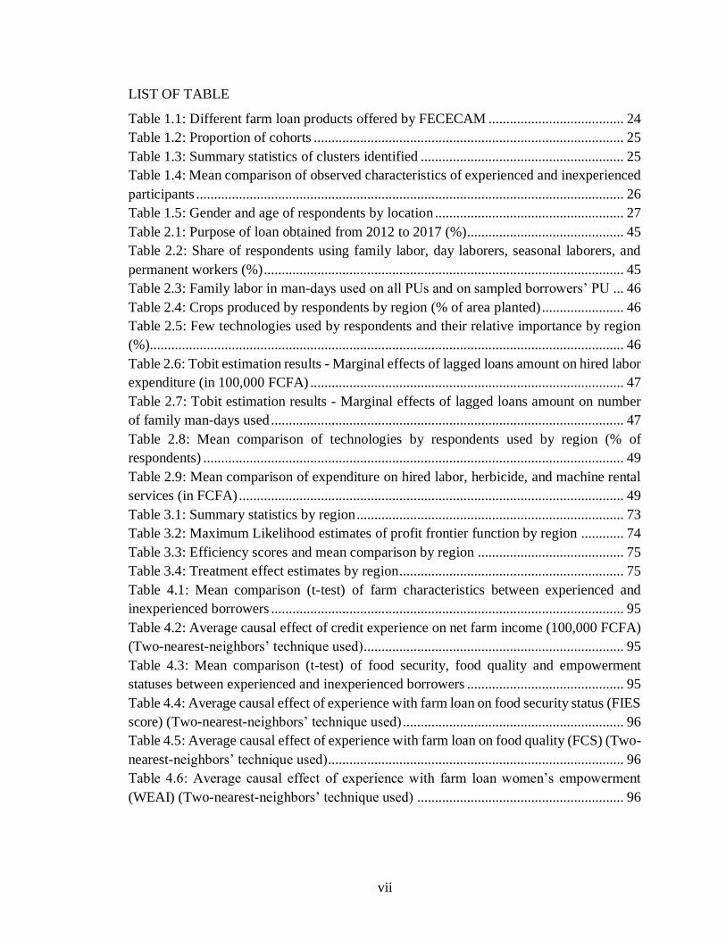
TABLE OF CONTENT

ACKNOWLEDGEMENTS ............................................................................................... iii

LIST OF TABLE .............................................................................................................. vii

LISTE OF FIGURES ....................................................................................................... viii

1. Introduction ............................................................................................................. 1

1.1. Motivation and objective .................................................................................... 1

1.2. Background and literature review ....................................................................... 3

1.2.1. Microfinance: definition and approaches.................................................... 3

1.2.2. Microfinance challenges ............................................................................. 4

1.2.3. Microfinance and risk management ............................................................ 5

1.2.4. History of microfinance in Benin ............................................................... 7

1.2.5. Types of microfinance institutions in Benin ............................................... 9

1.3. Presentation of the studied lender and its products ........................................... 10

1.3.1. Why FECECAM? ..................................................................................... 10

1.3.2. Loan products............................................................................................ 10

1.4. Survey design .................................................................................................... 12

1.4.1. Survey area, data collection, and data ....................................................... 12

1.4.2. Survey design ............................................................................................ 14

1.5. Impact assessment approach ............................................................................. 15

1.5.1. Brief notes on microfinance studies history.............................................. 15

1.5.2. Issues in identifying causal effects of microloans .................................... 16

1.5.3. Identification strategy ............................................................................... 18

1.6. Description of the sample and summary statistics ............................................ 21

1.6.1. Respondents’ characteristics ..................................................................... 21

1.6.2. Respondents’ household characteristics ................................................... 22

1.6.3. Credit history ............................................................................................ 23

Chapter 1 Tables and Figures ........................................................................................... 24

2.Agricultural loans and farm labor: a broader perspective on the impact of microcredit

........................................................................................................................................... 33

2.1. Introduction ....................................................................................................... 33

2.2. Farm household structure and labor use ........................................................... 35

2.3. Hypothesis of the chapter.................................................................................. 37

2.4. Methodology ..................................................................................................... 37

2.5. Results ............................................................................................................... 39

2.5.1. Descriptive analysis .................................................................................. 39

2.5.2. Agricultural loans and farm labor use ....................................................... 42

2.6. Conclusion ........................................................................................................ 44

Chapter 2 Tables and figures ............................................................................................ 45

vi

3.Does experience with agricultural loans improve farmers’ efficiency in Benin? A

stochastic frontier analysis ................................................................................................ 51

3.1. Introduction ....................................................................................................... 51

3.2. Conceptual framework ...................................................................................... 53

3.2.1. The concept of efficiency: definition and measurement ........................... 53

3.2.2. Agricultural loans and farmers’ efficiency ............................................... 55

3.3. Empirical framework ........................................................................................ 58

3.3.1. The profit frontier function ....................................................................... 58

3.3.2. Estimating the effect of loan experience on borrowers’ efficiency .......... 60

3.3.3. ATE versus ATET .................................................................................... 62

3.4. Results ............................................................................................................... 63

3.4.1. Data overview ........................................................................................... 63

3.4.2. Stochastic profit frontier estimation.......................................................... 65

3.4.3. Profit efficiency scores ............................................................................. 67

3.4.4. Agricultural loans and efficiency .............................................................. 68

3.5.Implications and Conclusion

....................................................................................................................................... 71

Chapter 3 Tables and figures ............................................................................................ 73

4.Impact of agricultural loans on farmers’ well being

........................................................................................................................................... 81

4.1. Introduction ....................................................................................................... 81

4.2. Theoretical framework ...................................................................................... 83

4.2.1. MFIs’ strategy and expected impact of microcredit ................................. 83

4.2.2. Microloan allocation as determinant of its impact .................................... 84

4.2.3. Conceptual role of agricultural credit ....................................................... 85

4.3. Impact estimation .............................................................................................. 86

4.4. Results ............................................................................................................... 88

4.4.1. Loan repurposing and loan sharing ........................................................... 88

4.4.2. Impact of loans experience on net farm income ....................................... 89

4.4.3. Impact of loans experience on Food security and nutritional status ......... 90

4.4.4. Impact of loans experience on women empowerment .............................. 92

4.5. Conclusion ........................................................................................................ 93

Chapter 4 Tables and Figures ........................................................................................... 95

General conclusion and discussion ................................................................................. 103

References ....................................................................................................................... 107

Vita .................................................................................................................................. 116

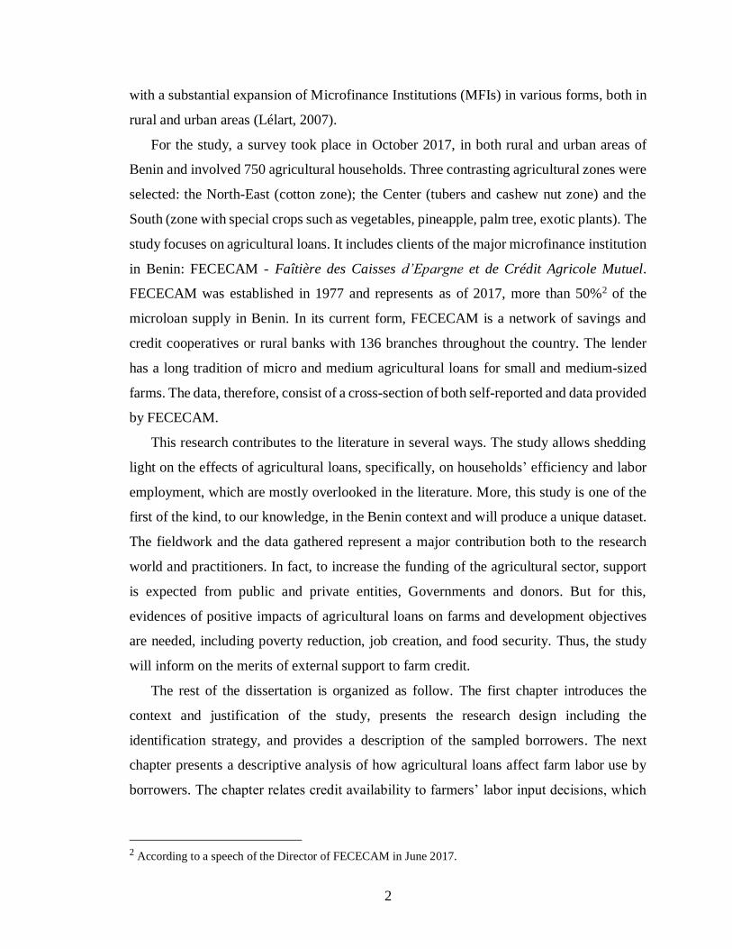
vii

LIST OF TABLE

Table 1.1: Different farm loan products offered by FECECAM ...................................... 24

Table 1.2: Proportion of cohorts ....................................................................................... 25

Table 1.3: Summary statistics of clusters identified ......................................................... 25

Table 1.4: Mean comparison of observed characteristics of experienced and inexperienced

participants ........................................................................................................................ 26

Table 1.5: Gender and age of respondents by location ..................................................... 27

Table 2.1: Purpose of loan obtained from 2012 to 2017 (%)............................................ 45

Table 2.2: Share of respondents using family labor, day laborers, seasonal laborers, and

permanent workers (%) ..................................................................................................... 45

Table 2.3: Family labor in man-days used on all PUs and on sampled borrowers’ PU ... 46

Table 2.4: Crops produced by respondents by region (% of area planted) ....................... 46

Table 2.5: Few technologies used by respondents and their relative importance by region

(%)..................................................................................................................................... 46

Table 2.6: Tobit estimation results - Marginal effects of lagged loans amount on hired labor

expenditure (in 100,000 FCFA) ........................................................................................ 47

Table 2.7: Tobit estimation results - Marginal effects of lagged loans amount on number

of family man-days used ................................................................................................... 47

Table 2.8: Mean comparison of technologies by respondents used by region (% of

respondents) ...................................................................................................................... 49

Table 2.9: Mean comparison of expenditure on hired labor, herbicide, and machine rental

services (in FCFA) ............................................................................................................ 49

Table 3.1: Summary statistics by region ........................................................................... 73

Table 3.2: Maximum Likelihood estimates of profit frontier function by region ............ 74

Table 3.3: Efficiency scores and mean comparison by region ......................................... 75

Table 3.4: Treatment effect estimates by region ............................................................... 75

Table 4.1: Mean comparison (t-test) of farm characteristics between experienced and

inexperienced borrowers ................................................................................................... 95

Table 4.2: Average causal effect of credit experience on net farm income (100,000 FCFA)

(Two-nearest-neighbors’ technique used)......................................................................... 95

Table 4.3: Mean comparison (t-test) of food security, food quality and empowerment

statuses between experienced and inexperienced borrowers ............................................ 95

Table 4.4: Average causal effect of experience with farm loan on food security status (FIES

score) (Two-nearest-neighbors’ technique used) .............................................................. 96

Table 4.5: Average causal effect of experience with farm loan on food quality (FCS) (Two-

nearest-neighbors’ technique used)................................................................................... 96

Table 4.6: Average causal effect of experience with farm loan women’s empowerment

(WEAI) (Two-nearest-neighbors’ technique used) .......................................................... 96

viii

LISTE OF FIGURES

Figure 1.1: Number of clients served by MFIs over time in Benin .................................. 28

Figure 1.2: Amount of savings deposited to MFI over time in Benin .............................. 28

Figure 1.3: Loan application timing during the studied period ........................................ 29

Figure 1.4: Distribution of respondents and sampled service points ................................ 30

Figure 1.5: Number of agricultural loan recipients between 2012 and 2017 in the population

and in the sample by studied region .................................................................................. 31

Figure 1.6: Number of years during which clients took loans by their entry time. .......... 31

Figure 1.7: Average years of schooling by gender and location....................................... 32

Figure 1.8: Amount of FECECAM loan received over time by region and gender ......... 32

Figure 2.1: Share of labor force employed in agriculture as a percentage of the total labor

force in Benin .................................................................................................................... 50

Figure 3.1: Contribution of farming activities to farmers’ income ................................... 76

Figure 3.2: Covariates balance diagnostic box plots and Kernel density plot using the

matched data in the North ................................................................................................. 76


matched data in the Center ................................................................................................ 77


matched data in the South ................................................................................................. 78

Figure 3.5: Estimated densities of predicted probabilities of getting each treatment level in

the North (overlap check) ................................................................................................. 79


the Center (overlap check) ................................................................................................ 79


the South (overlap check) ................................................................................................. 80

Figure 4.1: Shares of loan repurposed by region (%) ....................................................... 97


matched data (Net farm income)....................................................................................... 97


matched data (Food Insecurity Experience Scale) ............................................................ 98


matched data (Food Consumption Score) ......................................................................... 99


matched data (Women Empowerment in Agriculture Index) ......................................... 100

Figure 4.6: Overlap check for matching – Net farm income .......................................... 101

Figure 4.7: Overlap check for matching – FIES score.................................................... 101

Figure 4.8: Overlap check for matching – FCS score ..................................................... 102

Figure 4.9: Overlap check for matching – WEAI ........................................................... 102

1

1. Introduction

1.1. Motivation and objective

Since microfinance was conceived, it has generated a lot of hope for alleviating

poverty in low-income countries. Microfinance provides the poor with access to affordable

capital by granting low-income individuals with loans they would not otherwise have

access to, not only because of economic reasons but also because of geographic ones.

Microfinance also covers a variety of other products and services such as micro-savings,

microinsurance, transfers, leasing, as well as financial services training.

Microfinance, and more specifically, microcredit programs, have been supported

as sustainable interventions with the potential to alleviate poverty (Pankhurst and Johnston,

1999). However, the literature reveals discrepancies between what microfinance ought to

do, and what it actually does. More, evidence of the effectiveness of microfinance is still

unclear. On the one hand, studies show that microfinance does help the poor improve their

productivity or their well-being and enables them to pull out of poverty (Girabi and

Mwakaje, 2013; Otero, 1999; Pitt and Khandker, 1998). On the other hand, other studies

claim that evidence supporting the positive impact of microfinance interventions are thin

and lack rigor (Banerjee, Duflo, Glennerster, and Kinnan, 2014; Feder, Lau, Lin, and Luo,

1990; Roodman and Morduch, 2014).

The goal of this study is to examine the role and the importance of microfinance in the

agricultural sector of developing countries. More specifically, the study aims at assessing

the effects of agricultural loans on the rural world including farmers’ well-being,

production efficiency as well as their labor and technology use in the context of Benin—

in West Africa. Benin has made significant progress in improving access to financial

services over the past decades, and the country offers an interesting perspective for a

research on the subject. For the most part, financial service access points in Benin are

evenly distributed; there are no communes1 in the country that do not have at least one

access point. Indeed, most communes have at least six financial service providers present,

potentially indicating local competition (Brosnan, 2016). Moreover, Benin ranks among

the tops in microfinance in the West African Economic and Monetary Union (WAEMU),

1 Communes are the second administrative territorial divisions in Benin and there are seventy-seven (77)

communes in Benin.

2

with a substantial expansion of Microfinance Institutions (MFIs) in various forms, both in

rural and urban areas (Lélart, 2007).

For the study, a survey took place in October 2017, in both rural and urban areas of

Benin and involved 750 agricultural households. Three contrasting agricultural zones were

selected: the North-East (cotton zone); the Center (tubers and cashew nut zone) and the

South (zone with special crops such as vegetables, pineapple, palm tree, exotic plants). The

study focuses on agricultural loans. It includes clients of the major microfinance institution

in Benin: FECECAM - Faîtière des Caisses d’Epargne et de Crédit Agricole Mutuel.

FECECAM was established in 1977 and represents as of 2017, more than 50%2 of the

microloan supply in Benin. In its current form, FECECAM is a network of savings and

credit cooperatives or rural banks with 136 branches throughout the country. The lender

has a long tradition of micro and medium agricultural loans for small and medium-sized

farms. The data, therefore, consist of a cross-section of both self-reported and data provided

by FECECAM.

This research contributes to the literature in several ways. The study allows shedding

light on the effects of agricultural loans, specifically, on households’ efficiency and labor

employment, which are mostly overlooked in the literature. More, this study is one of the

first of the kind, to our knowledge, in the Benin context and will produce a unique dataset.

The fieldwork and the data gathered represent a major contribution both to the research

world and practitioners. In fact, to increase the funding of the agricultural sector, support

is expected from public and private entities, Governments and donors. But for this,

evidences of positive impacts of agricultural loans on farms and development objectives

are needed, including poverty reduction, job creation, and food security. Thus, the study

will inform on the merits of external support to farm credit.

The rest of the dissertation is organized as follow. The first chapter introduces the

context and justification of the study, presents the research design including the

identification strategy, and provides a description of the sampled borrowers. The next

chapter presents a descriptive analysis of how agricultural loans affect farm labor use by

borrowers. The chapter relates credit availability to farmers’ labor input decisions, which

2 According to a speech of the Director of FECECAM in June 2017.

3

pertain both to direct and indirect expected impact of farm credit. It also examines the

relation between labor and capital in the presence of farm loans. The third chapter of the

dissertation assesses the effect of agricultural loans on input allocation decisions and farm

profitability. It evaluates the impact of agricultural loans on the whole-farm efficiency of

borrowers in Benin. The fourth chapter assesses the impact of agricultural loans on

farmers’ well-being measured by their net farm income, nutritional and food security status

as well as women’s empowerment in agriculture index for female borrowers. Finally, a

general conclusion discusses the results of the dissertation and provide some

recommendations to different actors of the credit sector.

1.2.Background and literature review

1.2.1.Microfinance: definition and approaches

Microfinance is the provision of various financial services to the working poor.

Microcredit provides working poor with access to affordable capital by granting them loans

they would not otherwise have access to, because they do not meet both the economic and

geographic requirements of mainstream banks. Microfinance also covers a variety of other

products and services such as micro-savings, microinsurance, transfers, leasing, as well as

financial services training. This study focuses on microcredit and assesses its effect on

agricultural households.

Two divergent approaches dominate the current debates in the microfinance field:

the commercial approach or financial system approach and the poverty lending approach.

The commercial approach, which has a strong neoliberal groundwork, targets the

economically active poor–those with skills and earning capacity–and not the ultra-poor.

This approach is based on full cost-recovery, institutional self-sustainability and demand-

driven outreach principles (Batra, 2010). In contrast, the poverty lending approach, which

is the dominant paradigm in developing countries, targets the extremely poor to help them

out of poverty and gain empowerment. Under this approach, loans at below-market interest

rates are provided to the poor with funds from donors or governments. Even though the

approaches emphasize different aspects–on entrepreneurship and growth for the former,

and on poverty alleviation and empowerment for the latter–there is evidence that both

approaches contribute to the development of institutional microfinance (Batra, 2010). The

4

studied lender is a microfinance cooperative, which predominantly uses the financial

system approach. Though FECECAM has to cover its cost by ensuring financial

sustainability, the cooperative has a social component in its portfolio with very small loans

offered especially to poor women who benefit from group lending. These group loans come

with training and education on various aspects such as health, nutrition, and finance.

1.2.2.Microfinance challenges

In general, the microfinance sector face several challenges. One of the major challenges

faced by the sector resides in the fact that clients are hard to evaluate in terms of risk and

often costly to serve (Armendáriz de Aghion and Morduch, 2005). First, low-income

households, typically excluded from the formal banking system, lack collateral that a

financial institution needs in case of default. Second, mainstream banks tend to locate in

urban centers while most of the poor in developing world live in rural areas. Consequently,

the administrative costs of serving these rural clients are very high making it less profitable

(Ellrich and Sarges, 2010). The fixed cost of lending is therefore too high for small loans,

especially in rural areas. Third, creditors do not have complete information about the

borrowers. Either adverse selection occurs and banks cannot easily determine riskier

customers from safer and charge them accordingly, and/or moral hazard arises and lenders

are unable to ensure that customers are doing their best to make their investment projects

successful. In developing countries, weak judicial systems worsen these problems because

of the difficulty to enforce contracts (Armendáriz de Aghion and Morduch, 2005).

Several mechanisms have been developed to cope with these challenges. A standard

tool used involves requiring borrowers to apply for credit in voluntarily formed groups:

assuming that borrowers have better information about each other and will avoid higher

risk members (Armendáriz de Aghion and Morduch, 2005). The key feature of group

lending is the so-called joint liability (Stiglitz, 1990). According to this principle, all group

members are treated as being in default if a single member does not repay his loan. This

model was first used by the Grameen Bank in Bangladesh. In Benin, microfinance

institutions usually rely on group-based guarantees and women-led microcredits to cope

with the information asymmetry and the lack of collateral. However, while this promoted

5

the expansion at the early stage, it also contributed to the prevalence of unauthorized MFIs

(Cui, Dieterich, and Maino, 2016).

Several scholars point out the benefits of group lending (Armendáriz de Aghion and

Morduch, 2000; Godquin, 2004; Gomez and Santor, 2003; Guttman, 2007). For instance,

group meetings, through education and training, help clients with little experience improve

the financial performance of their businesses (Armendáriz de Aghion and Morduch, 2000).

Group lending plays a key role in mitigating risks associated with information asymmetry

(Godquin, 2004). Because group borrowers are jointly liable, they have the incentive to

monitor each other especially when one of them switches to a riskier project (moral

hazard). Therefore, peer pressure and social ties help reduce group members’ default

(Guttman, 2007). For instance, utilizing data from two North American microfinance

institutions, Gomez and Santor (2003) find evidence that those enrolled in group loans

programs outperform individual borrowers in terms of default probabilities. They attribute

that effect to the dual channels of sorting and incentives for greater effort once inside the

group.

However, there are negative aspects to introducing group lending (Armendáriz de

Aghion and Morduch, 2000; Besley and Coate, 1995; Kodongo and Kendi, 2013; Shankar,

2007). Group lending is often associated with additional costs such as group formation

costs, training costs of borrowers on group procedures, supervision and a higher frequency

of installment payments. The fact that all group members are penalized because of one or

few members represent an unappealing trait of group lending. Furthermore, merely

gathering good information does not guarantee contract enforcement or prevent strategic

default. Even when loan officers collect the necessary information before and after the loan

is given, they still face the problem of enforcing debt repayments once borrowers get their

investment’ returns. To circumvent the enforcement issue, most MFIs rely on dynamic

incentives; that is, good borrowers receive larger loans over time and defaulting ones incur

the risk of not receiving any more loans (Armendáriz de Aghion and Morduch, 2000).

1.2.3.Microfinance and risk management

Farmers in developing countries also face significant risk constraints along with capital

constraints. If lack of access to credit can limit farmers’ investment in activities with higher

6

profits, lack of access to formal insurance market can also prevent farmers from investing

in activities that may be risky but have high expected returns (Cai, Chen, Fang, and Zhou,

2015; Karlan, Osei, Osei-Akoto, and Udry, 2014).

Karlan et al. (2014) reported that farmers in northern Ghana most often cite lack of

capital as the reason why they have low farm investment, but they also understand the risk

of unpredictable rainfall and claim to reduce their farm investment because of it. The results

of their study show that capital constraints alone are not the problem but risk represents a

key hindrance to investment. The study concludes that the binding constraint to farmer

investment is uninsured risk as farmers are able to find resources to increase expenditure

on their farms when provided with insurance against the main catastrophic risk they face.

Microcredit networks and infrastructure could be used to construct better risk-

management tools. Although there has been some attempt at this, it has traditionally been

life insurance, not rainfall or a form of agricultural insurance (Karlan et al., 2014). Using

the first large-scale randomized experimental evidence of the effect of micro-insurance on

farmer production behavior, Cai et al. (2015) showed that micro-insurance may be as

important as microfinance in poverty alleviation, and that micro-insurance can supplement

and strengthen the effects of microfinance by protection the farmers from the inherent risk

of entrepreneurial activities.

For developing countries, agricultural insurance is not the “miracle solution” but it has

the potential to contribute to the development of more intensive and productive agricultural

systems by managing residual risks and securing income and credit programs. In western

African counties, crop insurances started very recently with the development of index

based crop insurance pilot projects in Mali and Burkina Faso (cotton, maize), Benin

(maize), and Senegal (groundnut, maize) (Muller et al., 2013). In those countries, the index

insurance pilot project covers farmers against rainfall deficit in order to protect them

against drought but also to protect financial institutions against the risk of default of their

borrowers.

In Benin, a local agricultural insurance institution has been created in 2007 to help farm

households cope with risk: the Agriculture Mutual Insurance of Benin (Assurance Mutuelle

Agricole du Bénin - AMAB). Besides the index insurance project for maize, AMAB offers

other products such as multi-risk harvest insurance, livestock mortality insurance,

7

agricultural facilities and warehouse insurance, health insurance (hospitalization) for

farmers, to name a few.

1.2.4.History of microfinance in Benin

The Republic of Benin is a small country in West Africa located between Nigeria and

Togo. Its total area is 112,622 sq km (43483.58 sq mi). As of 2015, Benin has an estimated

population of 10.9 million inhabitants. During the 2011-2015 period, Benin's real gross

domestic product (GDP) growth increased from 4.6% in 2012 to 6.5% in 2014 and was

among the best in WAEMU countries (The World Bank, 2016). However, poverty remains

widespread and even rising in the country. In 2007, the national poverty rate in Benin is

estimated at 32.2% for the monetary poverty and 39.6% for the non-monetary incidence of

poverty (INSAE, 2009). According to The World Bank (2016), this rate rose to 40.1% in

2015.

Benin’s experience with microfinance started in 1977, when a network of local farm

co-operatives, Caisses Locales de Crédit Agricole Mutuel (CLCAM3)) was created along

with the national farm credit bank (Caisse Nationale de Crédit Agricole (CNCA)). The

initial goal of the CNCA was to provide savings and credit services to farmers, government

workers as well as business owners. The emergence of microfinance organizations as we

know them today in Benin is a more recent phenomenon, the result of a series of events.

First, in the mid-1980s, the West African Economic and Monetary Union (WAEMU or

Union) countries, including Benin, faced a severe economic and social crisis. Benin

experienced the bankruptcy of its banking system and the subsequent closure of all state

banks4 which led to a lack of funding sources for all key sectors of the economy

(Adechoubou, 1996). It is believed that the financial crisis resulted from excessive

government intervention in the financial system. Consequently, in the early 1990s, the

government undertook a series of reforms to create strict regulatory frameworks to support

the emergence of a competitive private financial sector (Joseph, 2002). The government

also pulled out of most state-owned enterprises.

3 Local farm co-operatives (CLCAM) were overseen by the national farm co-operatives’ network of Benin

which is FECECAM (Faitières des caisses d’Epargne et de Crédit Agricole Mutuel du Bénin) in its old form. 4 These include the CNCA in 1987, the Benin Bank for Development in 1989 and the Commercial Bank of

Benin in 1990.

8

This withdrawal of the government facilitated the emergence of many micro-

enterprises, most of them in the informal sector, whose financing needs were not taken into

account by the formal financial sector in reconstruction. The WAEMU authorities, with

the support of International Development Cooperation Agency (CID), therefore committed

to broadening the financial landscape of the Union by promoting MFIs,5 which are

designed to meet the diverse financial needs of the population. In Benin, as in the whole

Union, the microfinance sector is, therefore, regulated by a law called the PARMEC6 Act.

With this act, savings and credit unions, as well as cooperatives, can be approved and their

local affiliates officially recognized by the respective Ministries of Finance of the member

states. Since its adoption in 1993, the PARMEC Act has been a major tool for the

development of the microfinance sector in West Africa by securing the collection of

savings, helping to control credit management and contributing to the professionalization

of MFIs (PNUD-Bénin, 2007). In 2012, Benin updated the PARMEC Act. Thus, in Benin,

the operation of MFIs is now governed by the 2012 Act regulating MFIs.

As of June 30, 2017, the Ministry of Economy and Finance reported 98 registered MFIs

operating in Benin with 639 service locations throughout the country (MEF, 2017).

However, several other MFIs operate illegally in the country and including them brings the

number of service points in the country up to 800 (PLURIEX, 2011). During the period

2005 to 2015, the number of clients collectively served by MFIs increased from 687,000

to 1,825,000. These figures reflect the rapid growth of MFIs in Benin even if a significant

segment of the population remains excluded from financial services. Figure 1.1 shows the

evolution of the number of clients over time.

As mentioned above, 78% of MFIs in Benin offer both credit and voluntary savings

opportunities to their clients. The amount of deposit has exponentially increased over the

last ten years. In 2005, clients’ deposits amounted 39.8 billion FCFA7 while in 2015

deposits were about 93.5 billion FCFA. Over the same ten years’ period, 74.2 billion FCFA

5 In Benin, MFIs are called decentralized financial systems (systèmes financiers décentralisés (SFD)).

FECECAM is a classical MFI with a greater regulatory oversight. 6 PARMEC stands for Projet d’Appui à la Réglementation des Mutuelles et Cooperatives d’Epargne et de

Crédit (Project to support the regulation of savings and credit unions and cooperatives) 7 1 USD 540 FCFA

9

of credit were disbursed by MFIs in 2005 and 124.03 billion FCFA in 2015 (MEF, 2016).

Figure 1.2 shows the amount deposited at MFIs over time in Benin

1.2.5. Types of microfinance institutions in Benin

There are several types of service providers in the microfinance sector in Benin. We

can classify microfinance institutions in terms of their mode of operation or their legal

status. In terms of legal status, two main categories exist:

- Unions and cooperatives of savings and credit: these are institutions incorporated

and licensed to provide microfinance services.

- Institutions non-incorporated as unions or cooperatives of savings and credit. These

institutions have their own legal status but also engage in microfinance activities.

However, these institutions are required to sign an agreement with the Ministry of

Finance which monitors their microfinance activities. Non-governmental Organizations

(NGOs), Microfinance companies (for-profit), and governmental programs or projects

are in this category.

When one considers the mode of operation, MFIs can be grouped into three main

categories (Amouzou, 2008; PNUD-Bénin, 2007).

- Credit and savings institutions: they offer both credit products and voluntary

savings. This type of institution includes unions and cooperatives as well as savings and

credit groups. According to the 2005 MFI census8, they represent 78% of the

microfinance institutions inventoried.

- Credit-only non-deposit taking institutions only grant credits, either from their own

credit lines or foreign partners. This category encompasses most associations and

microfinance companies. They represent about 18% of the MFI.

Organizations and projects with a microfinance component: they include non-

governmental organizations (microfinance NGOs) as well as government initiatives.

Programs of this kind operate either through direct credits to the population, or refinance

other MFIs. Microfinance projects account for approximately 3% of microfinance

initiatives at the national level.

8 Inventory done by the Microfinance Unit of the Ministry of Economy and Finance in 2005

10

1.3. Presentation of the studied lender and its products

1.3.1.Why FECECAM?

Established in 1977, FECECAM is the largest microlender in Benin and represents

more than 50%9 of the microloan supply in the country. In its current structure, FECECAM

is a network of savings and credit cooperatives that has the highest geographical coverage

with its 136 branches throughout the country. It has a long tradition of small and medium-

sized loans for farmers and agricultural businesses. FECECAM has been through multiple

crises over the years that led the network to neglect the agricultural credit line in past

decades for both internal and external reasons. The Federal German Ministry of Economic

Cooperation and Development (BMZ), through the German Financial Cooperation (KfW),

recently refinanced FECECAM with the aim of supporting rural credit in general and

agricultural credit in particular. At the same time, through its technical branch of

Cooperation (GIZ), the BMZ also finances technical support to farmers to facilitate their

applying for, using, and repaying loans. In addition, the GIZ supports several agricultural

commodity chains in Benin that it has identified as being under served by credit

organizations. This is the main impetus behind the GIZ supporting financial institutions

that specifically serve agriculture. This study has been commissioned and funded by the

KfW.

1.3.2. Loan products

The refinancing and support from the German government enabled FECECAM to

renew its focus on farm loans. In 2017, the cooperative included more than 1.5 million

members and nearly 400,000 borrowers, with agricultural loans representing 20% of the

total amount of loan disbursed (77,000 agricultural borrowers).

FECECAM offers a fairly large range of credit types and repayment options to meet

the diverse needs of both rural and urban clients. Credit types vary from short term (6 to

12 months) to long-term loans. The lender offers both individual and group loans of

variable sizes to its agricultural clients. In fact, the MFI offers different type of loans for

9 According to a speech of the Director of FECECAM in June 2017.

11

different agricultural activities or periods. For example, FECECAM offers loans for inputs

purchase, planting, harvest, storage costs, as well as for warrantage10. Even the repayment

options for agricultural loans are tailored to the cycle of the crop or the activity.

Table 1.1 summarizes the different types of agricultural loans. Note that the sample

includes all loan products listed in the table.

FECECAM requires its clients to reside in the commune of the service point where

they apply for a loan. Since FECECAM is a cooperative, it requires loan applicants to pay

a one-time membership fee of 500 FCFA (0.90 USD). Loan applicants must also provide

a member share of 1,000 FCFA. Applicants must also pay a 1,000 FCFA deposit fee for

every 50,000 FCFA borrowed, but these deposits count toward repayment. In most cases,

applicants must be members of FECECAM for at least three months prior to applying for

a loan. They must also have a minimum savings of 20% of the amount requested. Only

small size loans offered in groups are exempt11 from these rules.

Additional loan amounts can be requested only if borrowers have repaid any

previous loans, with the exception of farm loans obtained for specific agricultural activities;

for example, a loan for planting can be followed by a loan for harvest even if the former

loan is not fully repaid.

Generally, any amount of loan requested at FECECAM requires a (financial)

collateral of 15% to 20% of the amount requested, depending on the service point. This

requirement is in addition to the required minimum account balance mentioned above.

FECECAM only requires asset collateral (e.g., land titles and other assets) for individual

loans above 400,000 FCFA. In case of group loans, joint liability serves as the guarantee.

Some loans products come with technical support or training. For instance, with a

product such the agricultural loan for rural women – CAFER (Crédit Agricole aux Femmes

Rurales), women receive training in areas such as health, education, and production. A

group facilitator and loan agent appointed by FECECAM regularly meets with the loan

10 The “warrantage” or inventory credit system allows farmers to use their harvest as collateral to obtain a

loan rather than selling it at one at harvest, when prices are often low. This system was used by European

farmers in the 19th century. 11 Though, the one-time membership fee of 500 FCFA is paid by the group as a whole, not by the members

individually.

12

recipients to supervised and train them. She also collects the repayment installments when

they are due.

Overall, FECECAM agricultural credit program resembles a supervised credit

program. In a supervised agricultural credit scheme, farmers receive credit in the form of

an integrated package of financial support, technical guidance, as well as some inputs

supply. More details about supervised credit programs can be found in Brake (1974) and

Mohsin, Ahmad, and Anwar (2011). Before FECECAM’s approval, the farmer and the

credit agent make a farm (business) plan as well as a home plan. The home plan includes

average monthly expenditures and forecasted changes during the loan cycle. The farm plan

focuses on the operation to fund but also includes other farm activities that may generate

income or benefit the funded activities. Through the plan, farmers are directed and advised.

Certain commodities are promoted for their local economic potential and others are

discouraged or disapproved12. The supervised component of FECECAM credit program is

discussed further in the dissertation.

As Figure 1.3 shows, over our six-year study period, credit applications consistently

peak around the month of June. This is because the agricultural season, or the rainy season,

in all regions of the country starts around that period.

1.4. Survey design

1.4.1.Survey area, data collection, and data

The core of the dissertation is a survey of FECECAM agricultural borrowers in three

agricultural zones13 in Benin. Not having the means to cover all agricultural zones in Benin,

three contrasting agricultural zones were chosen: the North-East (cotton zone); the Central

(tubers and cashew nut zone); and South (zone with specialty crops such as vegetables,

pineapple, palm tree, and ornamental plants). The survey was conducted in 30 FECECAM

service points, covering 48 of the 77 communes of the country. On average, respondents

12 For instance, in Benin the sale of adulterated gasoline is a common activity, even though forbidden.

FECECAM does not fund such activities. 13 The Ministry of Agriculture of Benin had divided the country into seven different agricultural zones based

on their agro-ecology and their potential in terms of commodities chain development. These zones have been

called pôles de développement agricole (agricultural development poles).

13

live 25 km (16 miles) from their service points. Figure 1.4 shows the distribution of

respondents and sampled services points.

The fieldwork took place in October 2017 and collected information about the 2016-

2017 agricultural season. The data collection concerned several aspects of the borrowers’

life and activities. The questionnaire comprises ten key modules. The first module collects

information about the borrower’s identification and socio-economic characteristics such as

age, sex, status in their household, educational level, activities conducted and their

contribution to the respondents’ income over the studied period. The second module

enquires about sampled borrowers’ household composition as well as the time use of each

household member during the 2016-2017 agricultural season. Time use information

concerns mainly the time allocated to own productive activities as well as the time spent

working on the borrower’s farm or other household member’s farm. The third module

investigates the credit history of the respondents asking information such as the loan

obtained from FECECAM and other MFI, when they were obtained, the respective amount

of the loans, the funded activities, etc. It then focuses on details about the latest loan

obtained from FECECAM and its terms as well as its utilization. That module also collect

data on clients’ satisfaction of FECECAM’s loan program. The fourth module of the survey

questionnaire is about crop production inputs and outputs costs and quantities. The module

also includes land availability and land tenure. The fifth module contains information about

inputs and outputs costs and quantities of trade and processing activities. Next, the same

type of information is collected for livestock and animal husbandry. Other types of income

generating activities output and expenses are captured in a separate module. Labor use

during the studied agricultural season is the subject of a separate module. The module’s

questions are related to the labor type, labor quantity, work time, pay and type of contract,

geographical origin of workers among other questions. The ninth module enquires about

sampled borrowers’ assets type and values (household durable goods and productive asset).

The tenth module helps uncover borrowers’ household food security and nutritional

statuses as well as lean season information and coping mechanism. Note that these

questions are asked to female borrowers directly or spouses in case when the sampled

respondent is male. Finally, the survey closes with questions about sampled respondents’

14

perception of the impact of FECECAM loans on their activities as well as key outcome

variables.

Overall, the dissertation draws upon three sources of data: a questionnaire-based

survey of the sampled FECECAM clients, secondary data drawn from the FECECAM’s

database of agricultural borrowers, and a set of focus group discussions with the staff in

the local branches.

1.4.2.Survey design

Identification and estimation of the effects of microcredit participation are difficult

because of two levels of selection: self-selection into a microfinance program by the

households, and the screening process of MFIs. To address these biases, this study employs

the so-called pipeline design, which is typically used in cross-sectional setting in the

absence of fully randomized experiments. This approach is justified by the fact that both

its control and treatment groups consist of individuals who have chosen to participate in

the microfinance program, addressing these two major sources of selection bias.

The sample was drawn from the FECECAM borrowers’ database. First, the population

of interest was narrowed down to individuals who borrowed from FECECAM for

agricultural reasons from 2012 to 2017. This group includes borrowers who took a loan for

crop production, animal husbandry, the processing of agricultural products, and trade in

agricultural commodities. Then, a two-stage sampling approach was followed, with

representative geographical areas selected in the first stage, and random sampling of

FECECAM clients in the second stage. In the first stage, three agricultural zones (strata)

were chosen and, from each zone, ten FECECAM branches (clusters) were drawn with a

probability proportional to its size (in terms of agricultural clientele), resulting in 30

branches being selected out of 93 in total. Finally, 26 borrowers, with 13 being “new” and

13 being “old” were randomly selected per FECECAM branch. Clients were considered

“old” if they had entered FECECAM loan program at least three years before the survey

and “new” if they had entered within the year prior the survey.

In total, 780 agricultural borrowers were sampled. However, issues encountered

during the data collection changed the ultimate ratio between old and new clients, and

reduced the sample size. First, several new clients who had yet to repay their loans confused

15

the survey with a loan recovery mission. Many were reluctant to be interviewed and in

some cases refused completely. Also, the data collection revealed that some borrowers

from the initial sampling list had never taken agricultural loans, especially in the branches

located in the South14. In some extreme cases, it was not even possible to reach the 26

agricultural borrowers targeted per branch. Either this was due to errors in the coding of

their files during the application, or some loan agents purposely mis-categorized some

clients’ files so that the client could benefit from the relatively laxer terms15 of some of the

agricultural loan products. Ultimately, the study sample comprised 748 usable

observations, with the composition being 29% new loan recipients (entered in 2016 and

2017) and 71% old borrowers. Figure 1.5 shows the number of agricultural loan recipients

between 2012 and 2017 in the population and in the sample by studied region.

1.5. Impact assessment approach

1.5.1.Brief notes on microfinance studies history

Key themes in microfinance research are asymmetric information and transaction

costs present in imperfect rural credit markets (Marr, 2012). The concept of joint liability

discussed above is the most studied aspect of several theoretical models. In spite of their

usefulness, these theoretical models provide little knowledge about the impact that

microfinance might have on its users as well various changes induced. Therefore, a second

tradition in microfinance started dealing with the issue of impact on clients. In the process,

researchers gradually shifted the focus from analyzing impacts on the microfinance-funded

enterprise alone, to including changes at the household and individual levels (assuming

non-separability between households’ production and consumption functions), to the study

of intra-household dynamics and gender empowerment, to looking at specific socio-

economic impacts such as employment, technology, child nutrition and food security and

to studying wider community impacts (Marr, 2012).

14 The South is a more urban area where agricultural activities are not as predominant compared to the other

areas. 15 FECECAM usually requires loan applicants to maintain a saving account with the cooperative for at least

three months before applying for a loan. However, that condition is not enforced in case of agricultural loans.

Also, most agricultural loans below a certain amount do not require collateral.

16

1.5.2.Issues in identifying causal effects of microloans

Determining causality in microfinance studies is challenging. The assessment of the

impact of a microloan program amounts to gauging how the program affected the

participants and changed their lives. The issue with microcredit evaluation is that, once a

person or a household makes the decision to participate in a loan program, it becomes

impossible to know how their lives might have evolved without that loan. In other words,

the biggest challenge in microfinance program evaluation is finding the counterfactual

(Odell, 2015). A reflexive attempt is the use of non-borrowers. However, this is

problematic because those who self-select into a loan program could be fundamentally

different from those who never seek to borrow. If these distinguishing characteristics

systematically affect the outcome variables, there is selection bias. Factors such as

management and entrepreneurial abilities, risk preferences, resourcefulness, and

trustworthiness—which are hard to measure–could explain differences between borrowers

and non-borrowers. In addition, factors such as own financial constraints, assets, or

technology use could also differentiate borrowers from non-borrowers. In fact, it could be

that those with greater assets or those with a bigger operation (higher levels of inputs use

and outputs) are the ones that get loans; or that the use of loans actually improves

productivity. The location of the ‘treatment’ itself could also explain differences between

borrowers and non-borrowers, as MFIs typically choose to locate themselves in accessible

areas or places with higher economic potential. On top of this, loan providers use

systematic loan-worthiness-screening criteria that distinguish clients from non-clients. Any

estimation of loan effects in the presence of these issues of self-selection and/or

endogenous program placement will yield biased parameter estimates. Thus, any

evaluation of a microfinance program must use different methods to come up with a

reliable estimate of the counterfactual.

For these reasons, in many settings, treatment effects estimated from Randomized

Control Trials (RCT) are considered the gold standard. With an RCT, loans would be

randomly assigned to some study participants (the treatment group) and not to others (the

control group), or loan services would be offered to some randomly-assigned communities,

and not to others. The fact that study participants are randomly assigned to one group or

another eliminates any systematic differences between the two groups and thus, any

17

observed differences in measured outcomes between the two groups can be attributed to

the credit or the treatment assigned. However, there are some criticisms about RTC and the

broader validity of their results is not yet guaranteed (Banerjee, Duflo, Glennerster, and

Kinnan, 2014; Karlan and Zinman, 2011). RCT are expensive to conduct and are often

criticized for studying impact over a relatively short duration. More germane to this study,

researchers argue that most RCT studies are conducted in areas where considerable

microfinance lending already exists (Rajbanshi, Huang, and Wydick, 2015). Results from

such studies should then not be generalized as the average impact of microfinance.

However, studies such as Crépon, Devoto, Duflo, and Parienté (2015) and Rajbanshi et al.

(2015) represent some of the first efforts to study the impact of microfinance in an area

where no MFI was previously operating.

This study uses a quasi-experimental approach. In these studies, strategies are used by

researchers to come up with a reliable control group without the use of random assignment.

A widely used technique in quasi-experimental studies is the so-called “pipeline design”.

This design compares a representative sample drawn from the population that has received

‘treatment’ with a sample drawn from a comparable population that is about to receive it

for the first time (i.e., the pipeline group) (Coleman, 1999, 2006; Copestake, Bhalotra, &

Johnson, 2001; Marr, 2012). The difficulty with the pipeline approach is that pipeline

groups used as proxy for control groups could still introduce some bias to the estimates.

However, it is considered to be an adequate alternative in cases where RCTs are not

feasible.

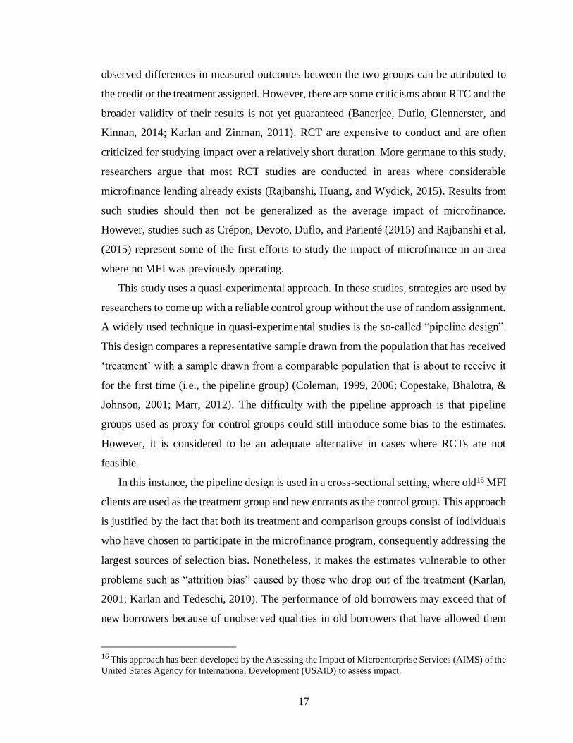
In this instance, the pipeline design is used in a cross-sectional setting, where old16 MFI

clients are used as the treatment group and new entrants as the control group. This approach

is justified by the fact that both its treatment and comparison groups consist of individuals

who have chosen to participate in the microfinance program, consequently addressing the

largest sources of selection bias. Nonetheless, it makes the estimates vulnerable to other

problems such as “attrition bias” caused by those who drop out of the treatment (Karlan,

2001; Karlan and Tedeschi, 2010). The performance of old borrowers may exceed that of

new borrowers because of unobserved qualities in old borrowers that have allowed them

16 This approach has been developed by the Assessing the Impact of Microenterprise Services (AIMS) of the

United States Agency for International Development (USAID) to assess impact.

18

to remain in the program. As a solution, Karlan (2001) suggests altering the veteran group

to include those who drop out. The authors argue that this small correction can significantly

improve the accuracy and therefore the reliability of the results.

1.5.3.Identification strategy

This research is based on data from a survey of FECECAM agricultural borrowers

conducted in October 2017.The survey focuses on recipients who have been borrowing

from the MFI for agricultural related reasons, at least since 2012. The sample includes

some borrowers who had entered the program even before 2012 and borrowers who joined

FECECAM from 2012 to 2017 (Table 1.2). By construction, the dataset retains all

‘dropouts;’ among the sampled clients, some have stayed ever since their entry and have

taken loans multiple times (during several years) while others have dropped out after one

or few loans. Over the six-year study period, the sampled borrowers have taken loans on

average 3.11 (1.75) times. For example, among participants who entered the program in

2012 and 2013 there are, respectively, 1.39% and 5.75% who borrowed only during one

year, 11.11% and 4.60% who borrowed during two years, 15.28% and 14.94% who

borrowed from FECECAM during three years. Over this period, FECECAM has had a

fairly stable operation and no new service point was opened. From a statistical point of

view, this is fortunate as the propensity to enter did not change and new clients make a

good comparison group for older ones, holding everything else constant.

Figure 1.6 presents the number of years during which the participants took loans, after

their entry in the program.

This variation in the actual lending period or frequency of borrowing, allowed by

the relatively long period considered, introduces a complication into dividing the sample

into old and new clients just based on the time of entry as done by previous studies that

used the cohort approach. In fact, as confirmed by figure 5, not all early clients borrowed

for long. Put differently, not all early clients have the same experience with FECECAM

credit program. In fact, participants have borrowed variable amounts between 2012 and

2017, and they have also borrowed several times, even within a year. In this context,

program entry timing cannot solely determine the experience with loan from 2012 to 2017,

which is the loan treatment here. An early entry increases participants’ likelihood to be

19

experienced as they are more exposed, but it does not exclusively determine their

experience with loans.

A better definition of participants experience with loans would involve (i) the time

since the first loan, which captures seniority, (ii) the number of loans received, to capture

regularity, and (iii) the average amount of credit obtained over the period in question, to

apprehend intensity. Therefore, the loan treatment in this study is captured using a

combination of program entry timing, cumulative loan amounts, and the number of loans

taken between 2012 and 2017. However it is measured, the effect of loans on a household

is expected to build over time. For experienced clients, benefits from loan program

participation would have already accrued over a certain period, say six years, while

inexperienced clients would see little to no benefit depending on the time between their

loan receipt and the reference period. The appropriateness of this approach rests on the

absence of systematic differences between experienced and inexperienced borrowers.

Consequently, differences in studied outcome variables between the two groups of clients

can be attributed to credit, after controlling for factors such as demographics and

environment.

Survey respondents received loans from other sources as well. However, only 5.2%

of the respondents took additional loans from other formal MFIs during the period

considered, while the majority, 94.6% of respondents, received loans exclusively from

FECECAM, and 0.2% of the respondents took additional loans from informal sources such

as moneylenders, relatives and friends. Thus, while the average loan size includes amounts

received from other formal MFI during the considered period,17 the loan effect is

effectively the FECECAM agricultural loan effect.

On average, respondents have joined FECECAM 5.58 years prior to the survey.

They have obtained a loan three times already and have borrowed a total amount of

1,727,400 FCFA on average between January 2012 and October 2017. For a better

grouping and description of the sample based on the loan treatment, a k-means cluster

analysis is performed. Cluster analysis is an exploratory data-analysis technique which uses

17 In their review of 11 studies on credit studies, Gaile and Foster (1996) have pointed out the lack of

including or mentioning the presence or absence of possibly competing financial institutions in the studied

areas.

20

an algorithm to determine the natural groupings (or clusters) of observations. In this

specific case, the k-means clustering defines groups by minimizing the heterogeneity of

individuals within those groups. The number of (non-overlapping) groups to be created is

specified by the user. For a more detailed description of the algorithm, the reader is directed

to Makles (2012).

Table 1.3 summarizes the results of the k-means cluster analysis. We specify two

groups, with the expectation that this would divide the sample into experienced borrowers

and inexperienced borrowers. The first group includes borrowers, who, on average from

2012 to 2017, have joined FECECAM 15 years prior to the study, have taken a loan four

times and have received an average of 1,126,000 FCFA of loan each time. The second

group consists of borrowers, who, on average, entered the loan program only three years

before the study, have taken two to three loans, and have received an average amount of

300,000 FCFA of loan each time they have borrowed. Indeed, we can call the first group

the experienced borrowers while the second cluster can be called the inexperienced

borrowers.

One can argue now that there is less heterogeneity within each group in comparison.

Looking at characteristics other than those listed in table 1.3 for each of the two groups

confirms that there are no critical differences between the two groups (Table 1.4).

Experienced participants seem to be “an older version’’ of the inexperienced ones. In fact,

experienced borrowers are older, therefore, they are mostly household heads, they have

bigger household size, and they have been conducting their autonomous activities for

longer. In addition, inexperienced borrowers seem to live farther from FECECAM service

points than the experienced ones, which indicates that FECECAM is reaching farmers in

remote areas as well. Admittedly, experienced borrowers are more educated than

inexperienced ones. Nevertheless, no variable indicates critical differences between the

two groups. Most differences are age-related. Matching methods will help eliminate these

minor dissimilarities between the two groups, in order to estimate the causal effect of loan

experience.

21

1.6. Description of the sample and summary statistics

1.6.1.Respondents’ characteristics

Age and gender

Table 1.5. summarizes the proportion of male and female respondents as well as

their average age by region. On average, sampled borrowers are 44 years old. This average

age is consistent across gender and regions.

The sample includes 32.22 % of female borrowers and 67.78 % of male. The Center

has the highest proportion of female respondents (40.64%). The lowest percentage of

female borrowers is in the South, and this is partly explained by socio-cultural differences.

In the South, women are less involved in agricultural activities. Also, para -agricultural

activities such petty trade and processing of agricultural commodities in which women are

mostly involved in this area is relatively less funded by agricultural lenders.

Education

Respondents level of education is measured using their years of schooling, which

is the total number of years passing to the next grade level. The average number of years

of schooling is low (see figure 1.7). It increases from the North to the South and male

recipients are more educated than female recipients. On average, the respondents have not

finished their primary school. It’s only in the South that a substantial proportion of

recipients have finished at least primary education.

Education level was also assessed using respondents’ ability to communicate in

French18. In fact, even though loan agents can speak the local languages, loan application

documents as well as all administrative paperwork are written in French. Therefore,

proficiency in French (speaking at least) is important. Yet, only 19.54% of the recipients

can easily communicate in French. The South has the highest proportion of borrowers with

good proficiency in French speaking while the North has the lowest rate. This confirms the

finding (figure 1.7) that respondents in the South are more educated compared to other

regions. There are twice less women fluent in French as men (11.76% versus 23.21%).

18 French is the official language of Benin.

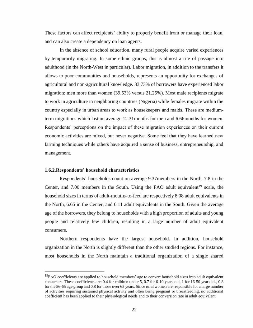
22

These factors can affect recipients’ ability to properly benefit from or manage their loan,

and can also create a dependency on loan agents.

In the absence of school education, many rural people acquire varied experiences

by temporarily migrating. In some ethnic groups, this is almost a rite of passage into

adulthood (in the North-West in particular). Labor migration, in addition to the transfers it

allows to poor communities and households, represents an opportunity for exchanges of

agricultural and non-agricultural knowledge. 33.73% of borrowers have experienced labor

migration; men more than women (39.53% versus 21.25%). Most male recipients migrate

to work in agriculture in neighboring countries (Nigeria) while females migrate within the

country especially in urban areas to work as housekeepers and maids. These are medium-

term migrations which last on average 12.31months for men and 6.66months for women.

Respondents’ perceptions on the impact of these migration experiences on their current

economic activities are mixed, but never negative. Some feel that they have learned new

farming techniques while others have acquired a sense of business, entrepreneurship, and

management.

1.6.2.Respondents’ household characteristics

Respondents’ households count on average 9.37members in the North, 7.8 in the

Center, and 7.00 members in the South. Using the FAO adult equivalent19 scale, the

household sizes in terms of adult-mouths-to-feed are respectively 8.08 adult equivalents in

the North, 6.65 in the Center, and 6.11 adult equivalents in the South. Given the average

age of the borrowers, they belong to households with a high proportion of adults and young

people and relatively few children, resulting in a large number of adult equivalent

consumers.

Northern respondents have the largest household. In addition, household

organization in the North is slightly different than the other studied regions. For instance,

most households in the North maintain a traditional organization of a single shared

19FAO coefficients are applied to household members’ age to convert household sizes into adult equivalent

consumers. These coefficients are: 0.4 for children under 5, 0.7 for 6-10 years old, 1 for 16-50 year olds, 0.8

for the 56-65 age group and 0.8 for those over 65 years. Since rural women are responsible for a large number

of activities requiring sustained physical activity and often being pregnant or breastfeeding, no additional

coefficient has been applied to their physiological needs and to their conversion rate in adult equivalent.

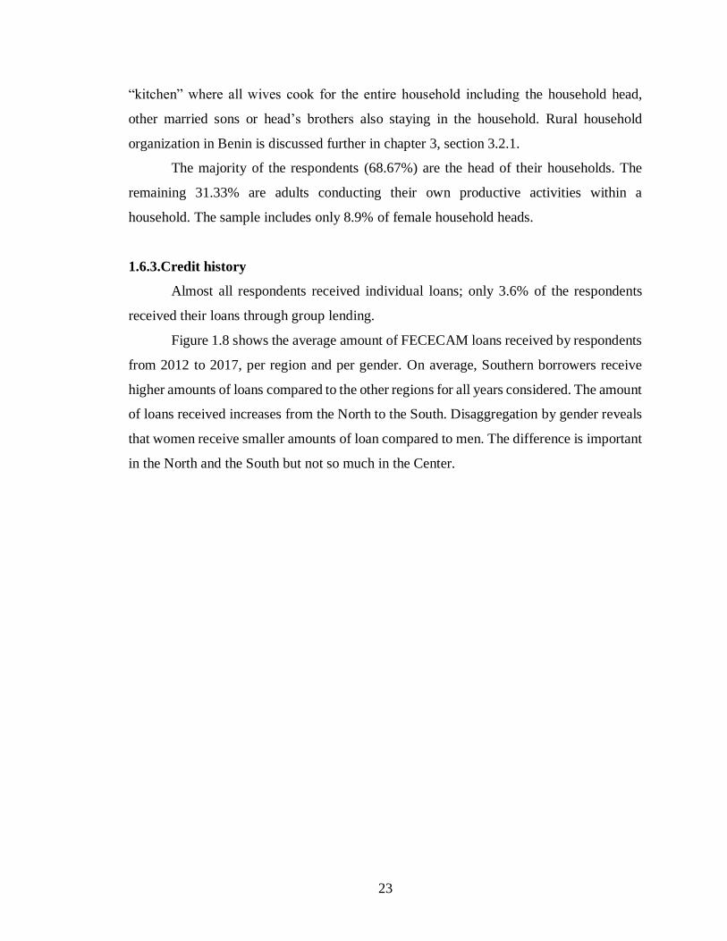
23

“kitchen” where all wives cook for the entire household including the household head,

other married sons or head’s brothers also staying in the household. Rural household

organization in Benin is discussed further in chapter 3, section 3.2.1.

The majority of the respondents (68.67%) are the head of their households. The

remaining 31.33% are adults conducting their own productive activities within a

household. The sample includes only 8.9% of female household heads.

1.6.3.Credit history

Almost all respondents received individual loans; only 3.6% of the respondents

received their loans through group lending.

Figure 1.8 shows the average amount of FECECAM loans received by respondents

from 2012 to 2017, per region and per gender. On average, Southern borrowers receive

higher amounts of loans compared to the other regions for all years considered. The amount

of loans received increases from the North to the South. Disaggregation by gender reveals

that women receive smaller amounts of loan compared to men. The difference is important

in the North and the South but not so much in the Center.

24

Chapter 1 Tables and Figures

Table 1.1: Different farm loan products offered by FECECAM

Loan products Amounts

Annual

interest

rates

Duration Individual /

Group

TPCF - Tout Petit Crédit aux

Femmes (tiny loans for women) 10,000 FCFA20 19%

0-12

months

Group loans but

given individually

TPCH - Tout Petit Crédit aux

Hommes (tiny loans for men) 10,000 FCFA 19%

0-12

months

Group loans but

given individually

CEE - Crédit Épargne avec

Education (savings-credit with

education)

30,000 –

400,000 FCFA 19%

6-12

months

Group loans but

given individually

for women

CAFER - Crédit Agricole aux

Femmes Rurales (agricultural

loans for women in rural areas)

30,000–

450,000 FCFA 19%

0-12

months

Group loans but

given individually

CFC - Crédit aux Femmes

Commerçantes (loans for female

small businesses)

30,000–

400,000 FCFA 19%

0-12

months Individual loans

CAEP - Crédit à l’Agriculture ; à

l’Elevage et à la Pêche (loans for

crop production, livestock, and

fishing)

10,000-5M

FCFA

19%

Short-

term: 0-

12months

Individual and

group loans

30,000-30M

FCFA

18%

Mid-term:

24-36

months

30,000-30M

FCFA 18%

Long-

term: 36-

120

months Source: FECECAM

20 1 US dollar is approximately 550 FCFA (1 FCFA ≈ 0.0018 USD)

25

Table 1.2: Proportion of cohorts

Cohort Share in sample (%)

Before 2012 29.01

Entered in 2012 9.49






Total 100

Table 1.3: Summary statistics of clusters identified

Variable

Group 1

Experienced

borrowers

Group 2

Inexperienced

borrowers

All

Average loan size over the studied period

(100,000 FCFA) 11.26 (12.63) 3.02 (2.61) 4.70 (7.00)

Number of loans between 2012 and 2017 4.05 (1.77) 2.87 (1.67) 3.11 (1.76)

Time since first loan with FECECAM21 (Years) 15.16 (7.33) 3.12 (2.83) 5.58 (6.40)

Number of observations 153 595 748

Notes: The k-means cluster analysis uses the Euclidian distance as the measure of similarity (dissimilarity)

between observations.

21 The research accounts for other sources of formal loans. Thus, respondents were also asked about their

first formal loan with any other MFI. On average, they entered a formal MFI program since 5.83 (6±.85)

years. A two-sample t-test shows that there is no significant difference between the mean of the two variables:

time since first FECECAM loan and time since first formal loan. This also confirms that the majority of the

borrowers interviewed use FECECAM as their primary formal loan provider.

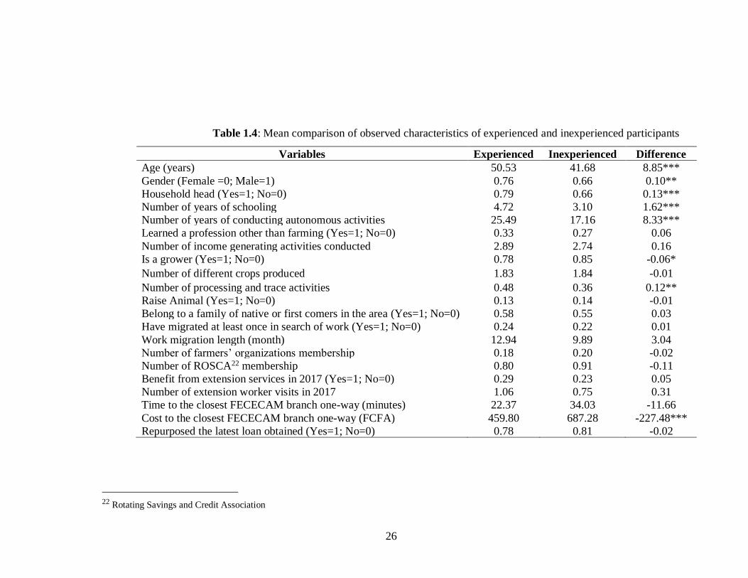
26

Table 1.4: Mean comparison of observed characteristics of experienced and inexperienced participants

Variables Experienced Inexperienced Difference

Age (years) 50.53 41.68 8.85***

Gender (Female =0; Male=1) 0.76 0.66 0.10**

Household head (Yes=1; No=0) 0.79 0.66 0.13***

Number of years of schooling 4.72 3.10 1.62***

Number of years of conducting autonomous activities 25.49 17.16 8.33***

Learned a profession other than farming (Yes=1; No=0) 0.33 0.27 0.06

Number of income generating activities conducted 2.89 2.74 0.16

Is a grower (Yes=1; No=0) 0.78 0.85 -0.06*

Number of different crops produced 1.83 1.84 -0.01

Number of processing and trace activities 0.48 0.36 0.12**

Raise Animal (Yes=1; No=0) 0.13 0.14 -0.01

Belong to a family of native or first comers in the area (Yes=1; No=0) 0.58 0.55 0.03

Have migrated at least once in search of work (Yes=1; No=0) 0.24 0.22 0.01

Work migration length (month) 12.94 9.89 3.04

Number of farmers’ organizations membership 0.18 0.20 -0.02

Number of ROSCA22 membership 0.80 0.91 -0.11

Benefit from extension services in 2017 (Yes=1; No=0) 0.29 0.23 0.05

Number of extension worker visits in 2017 1.06 0.75 0.31

Time to the closest FECECAM branch one-way (minutes) 22.37 34.03 -11.66

Cost to the closest FECECAM branch one-way (FCFA) 459.80 687.28 -227.48***

Repurposed the latest loan obtained (Yes=1; No=0) 0.78 0.81 -0.02

22 Rotating Savings and Credit Association

27

Table 1.4 (Continued): Mean comparison of observed characteristics of experienced and inexperienced

participants


Household characteristics

Household size 8.85 7.89 0.96***

Number of production unit heads23 2.57 2.33 0.24***

Number of consumption units (mouths to feed based on needs) (adult equivalent24) 7.79 6.76 1.03***

Number of cooking units25 1.52 1.26 0.25***

Total workforce available in the household based on member time allocation (adult

equivalent)

6.56 5.52 1.04***

Notes: *** p<0.01, **p<0.05, * p<0.1.

Table 1.5: Gender and age of respondents by location

Proportion (%) Age (years)

Female Male Female Male

North 27.52 72.48 43.68 (12.01) 42.53 (11.33)

Center 40.64 59.36 41.12 (9.88) 41.81 (12.83)

South 28.45 71.55 45.06 (9.51) 46.68 (10.33)

Total 32.22 67.78 42.99 (10.55) 43.72 (11.65)

23 A production unit is a homogenous unit within the farm household which has autonomy in terms of activity, decision, and resources use but which head

(household member and dependent) still reports to the household head. 24 To convert household members into adult equivalent consumers, we use FAO coefficients of conversion: 0.4 for children under 5, 0.7 for 6-10 years

old, 1 for 16-50 year olds, 0.8 for the 56-65 age group and 0.8 for those over 65 years. Since rural women are responsible for a large number of activities

requiring sustained physical activity and often being pregnant or breastfeeding, no additional coefficient has been affected for their physiological needs

and conversion rate in adult equivalent. 25 The “cooking units” or “kitchens” refer to distinct food management and food preparation units within a household

28

Figure 1.1: Number of clients served by MFIs over time in Benin

Source: Ministry of Economy and Finance, 2016

Figure 1.2: Amount of savings deposited to MFI over time in Benin

Source: Ministry of Economy and Finance, 2016

0

500

1000

1500

2000

2005 2006 2007 2008 2009 2010 2011 2012 2013 2014 2015

Number of MFI clients over time (in 1,000)

0

20

40

60

80

100

2005 2006 2007 2008 2009 2010 2011 2012 2013 2014 2015

Savings/deposits in MFI in billion FCFA

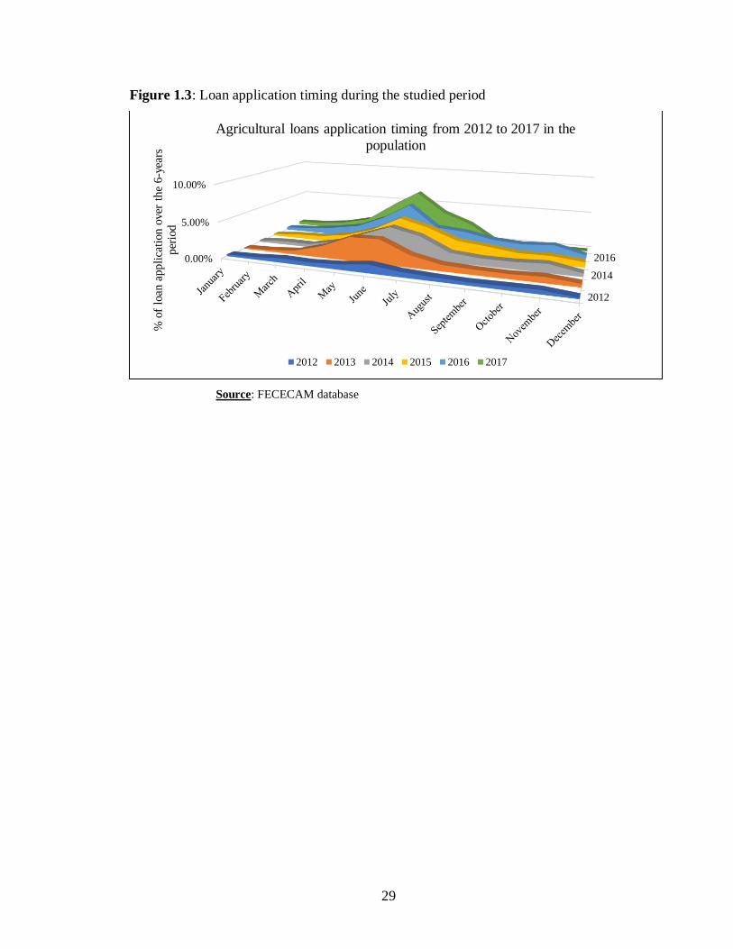
29

Figure 1.3: Loan application timing during the studied period

Source: FECECAM database

2012

2014

20160.00%

5.00%

10.00%

% o

f lo

an a

pp

lica

tion o

ver

the

6-y

ears

per

iod

Agricultural loans application timing from 2012 to 2017 in the

population

2012 2013 2014 2015 2016 2017

30

Figure 1.4: Distribution of respondents and sampled service points

31

Figure 1.5: Number of agricultural loan recipients between 2012 and 2017 in the

population and in the sample by studied region26

Figure 1.6: Number of years during which clients took loans by their entry time.

26Borrowers in the South have been oversample in order to obtain the 26 recipients per service point like the

other regions.

0

2000

4000

6000

8000

10000

12000

14000

2012 2013 2014 2015 2016 2017

Ag loans recipients in the population

North-East Center South

0

50

100

150

200

250

2012 2013 2014 2015 2016 2017

Ag loans recipients in the sample

North-East Center South

0 20 40 60 80 100

Before 2012

Entered in 2012

Entered in 2013

Entered in 2014

Entered in 2015

Entered in 2016

Entered in 2017

Number of years of borrowing by year

of the first loan

6years 5 years 4 years 3 years 2 years 1 year

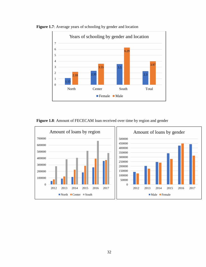
32

Figure 1.7: Average years of schooling by gender and location

Figure 1.8: Amount of FECECAM loan received over time by region and gender

1.13

2.35

3.5

2.32.18

3.55

6.29

3.97

0

1

2

3

4

5

6

7

North Center South Total

Years of schooling by gender and location

Female Male

0

50000

100000

150000

200000

250000

300000

350000

400000

450000

500000

2012 2013 2014 2015 2016 2017

Amount of loans by gender

Male Female

0

100000

200000

300000

400000

500000

600000

700000

2012 2013 2014 2015 2016 2017

Amount of loans by region

North Center South

33

2. Agricultural loans and farm labor: a broader perspective on the impact of

microcredit

2.1.Introduction

The agricultural sector continues to play a significant role in the development of low-

income countries. The sector represents a significant part of the economy of these countries

in terms of both aggregate income and total labor force. By generating income and

employment in rural areas, agriculture contributes to both poverty reduction and income

growth in developing countries where nearly 60% of the labor force is employed in

agriculture (Dethier and Effenberger, 2012).

Population growth is projected to keep its upward trend and highest population growth

rates will continue to be in developing regions for the coming decades (UN-DESA, 2010).

This rapid growth of the population places higher demands on global agricultural

production. According to the theory of intensification of farming systems developed by

Boserup (1965) and Ruthenberg (1971), the BR model of intensification, population

growth provides the necessity for agricultural intensification, while market access created

by rapid urbanization and economic growth offer new opportunities. However, output

growth requires increased cost of labor and other inputs per farmed area (Binswanger-

Mkhize and Savastano, 2017). Moreover, agricultural productivity growth drives not only

increased factors use but also the adoption of technology by farmers, e.g. land-saving

technologies such as organic manure and fertilizer to offset declining soil fertility or labor-

saving technologies such as machines.

Most intensification and modernization pathways require funding, which is not always

available to farmers in developing countries, especially the smallholders. Thus, rural credit

market has a crucial role to play in factor markets as it provides working poor with access

to affordable capital to acquire the needed inputs.

The objective of this chapter is to relate credit availability to farmers’ labor input

decisions. Rural wage labor market has the potential to develop economic linkages between

the small pool of households owning large shares of productive land and the remaining

landless or those with limited access to land but with excess labor. Thus, rural labor market

could serve as an important pathway out of poverty enabling resource-poor farmers with

34

excess labor to earn wage income and improve their economic well-being. More, credit

provision could also play an important role on the rural labor market by allowing farmers

to purchase the inputs they need, including labor. In developing countries, job creation is a

major concern for policymakers. In these countries where agriculture represents an

important source of livelihood and a sizeable share of the economy, farm labor market

represents a significant source of employment opportunity.

The agricultural sector in Benin is dominated by small to medium farm households

conducting polyculture often associated with small livestock (poultry, small ruminants, or

pigs). These farm households count on average seven members and farm 1.7 ha of land.

Only 5% of farms in the South and 20% in the North exploit more than 5 ha (MAEP, 2011).

Given the small farm sizes and other economic constraints, agriculture is operated

predominantly by human power–76% of land preparation is done manually and 23% by

animal draft. Figure 4.1. depicts the percentages of labor force employed in agriculture

over time in Benin.

The relevance of a study on the effects of agricultural loans on farm labor use can be

easily established. Several scholars feared that agricultural intensification may worsen the

conditions of smallholder farmers in developing countries as large holders, not only, may

grab their land, but also invest in labor-saving technologies, leaving landless farmers with

excess labor unemployed. Finding evidence suggesting that agricultural loans foster labor

hiring in the sector would invalidate such hypothesis and reinsure stakeholders and actors

of both the agricultural and credit sectors.

The literature on the impact of microcredit on employment is very scant, and results

are very mixed. According to Erhardt (2017), the evidence of the effects on employment is

still limited for two reasons. First, the vast majority of evaluated programs are not designed

to create employment. Rather, they aim at increasing income and consumption, poverty

reduction or various other outcomes such as children school attendance or empowerment

of women. Second, those studies which do assess programs aiming at employment creation

are usually limited to the impact on self- employment. In the literature, only very few

evaluations investigate the impact of microfinance on labor demand and most of them focus

on child labor (e.g. Angelucci, Karlan, & Zinman, 2015; Banerjee, Duflo, Glennerster, &

Kinnan, 2014; Blume & Breyer, 2011; Hazarika & Sarangi, 2008).

35

In this chapter, a descriptive analysis of the role of agricultural loan in borrowers’ labor

input choices is performed. The chapter uses data of growers’ subsample. The analysis

does not claim causality but allows to examine how lagged farm loans received over the

studied period are correlated with farmers’ current labor use. Results suggest that past loans

have residual effects on both hired and family labor use of agricultural borrowers. Farm

loans, especially those obtained for farm machinery are significantly correlated with

reduction in hired labor expenditure. However, more family man-days are employed using

the machine loans while other loan categories reduce the use of family labor.

2.2. Farm household structure and labor use

Considering the full nature of a farm household socio-economic organization is

essential to understand how agricultural loans may affect farm households in general and

its labor use in particular.

The neoclassical agricultural household model conceives the farm household as a

production and consumption unit, which converts its resources as well as purchased goods

and services into values or utility when consumed (Becker, 1965; Lamarche, 1991;

Mendola, 2007; Taylor and Adelman, 2003).

Allocation within a farm household is similar to the allocation that takes place

within a firm. Most farm households have a hierarchical structure in which much of the

control over the household resources (land and capital) are concentrated in the hands of the

household head (Fafchamps, 2002). Beside an hierarchical structure, farm households

often establish an explicit division of labor along with a system of delegation of authority

(Fafchamps, 2002; Fafchamps and Quisumbing, 2003). The structure of farm households

in Benin is consistent with this model.

In Benin, there are several modes of social organization. The notion of household

varies depending on the country’s regions from a small household with a head, and his wife

(wives) and (their) children, to a household with multiple generations of “households” (for

example siblings or close relatives with their spouses and children), all living in the same

place, and reporting to the household head, often the elder. The case of Benin is similar to

those of other Sub-Saharan African countries described by Fafchamps (2002) who stated

that households in those countries are large and occasionally encompassing several couples

36

with their children. In parts of Benin, household members conduct multiple income

generating-activities both on their own account and in collaboration with others

(Fafchamps, 2002). The farm household engages in both market and non-market tasks such

as farming, animal husbandry, fishing, crafts, trades, processing, gathering (fruits, nuts,

fuelwood, water, etc.) (e.g. Fafchamps, 2002; Hunt, 1991). In Benin, as it is the case in

most developing countries, there are many children on the farm households and they spend

most of their time helping around the house or the farm. It is often argued that, the big size

of the farm household is motivated by the fact that both children and wives serve as labor

(Binswanger and McIntire, 1987; Fafchamps, 2002; Fafchamps and Quisumbing, 2003).

In Benin, the household is organized around a socially recognized head of

household and includes all permanent dependents (often relatives) and migrants sent

elsewhere for work or education/training but who maintain social and economic relations

with the household (provide it with resources or still depend on the head). The farm

household head controls most of the household resources; he allocates usufruct rights, and

to some extent, he controls the labor force of his dependents. These resources are allocated

to activities under his supervision or to those of his dependents (family workforces) who

also manage autonomous production units of variable size within the farm household. It is

important here to make the distinction between the household as a production unit (as

defined earlier in this chapter) and production units within a farm household. In this study,

a “production unit” (PU), is a homogenous unit within the farm household which has

autonomy in terms of activity, decision, and resources use but which head (household

member and dependent) still reports to the household head. The household head’s

production unit is considered the main production unit and it is often the largest PU within

the farm household. All the surveyed borrowers are production unit heads (PUH). 73.77%

are the heads of their household whereas 26.23% are adult dependents conducting their

own productive activities within the farm household.

In Benin, as in most African societies, there are detailed evolved laws and customs

governing the use and transfer of productive resources (land and capital) along with

specific tasks and role division among household members according to their status (e.g.

Fafchamps and Quisumbing, 2003). These rules ensure the welfare of the household as a

group by requiring work and economic participation from all members. For instance, all

37

dependents owe their labor to the household head (e.g. Iversen, 2002). Children also owe

their labor to their respective mother. The household head in return provides shelter to the

entire household, food27 to some extent and also provides pieces of land28 to each adult

dependent in case they farm on their own account. Young children in the household, often

male, may earn some pocket money or school fees by cultivating their own field, but they

must first work on the household head’s field. Fafchamps (2002) described similar

practices in his work on intra-household resources allocation. In Northern regions of Benin,

adult sons often work for the household head on his fields in exchange for shelter, food,

durable goods such as cellphones, radio, motor bikes, or for a full dowry or money to marry.

2.3. Hypothesis of the chapter

It is important to formulate hypotheses that will guide the conduct of this section of

the dissertation. The hypotheses are the following:

H1: Farmers in Benin reduce their family labor use in the presence of agricultural loans.

H2: Farmers in Benin use more hired labor when they receive agricultural loans.

2.4. Methodology

A key threat to identification in microfinance studies is selection bias. Our study

addresses this issue by using a cohort approach. The research is based on a cross-sectional

data from a survey of FECECAM agricultural borrowers conducted in October 2017.The

survey focuses on recipients who have been borrowing from the MFI for agricultural

related reasons, at least since 2012. The sample includes some borrowers who had entered

the program even before 2012 and borrowers who joined FECECAM from 2012 to 2017.

By construction, the dataset retains all ‘dropouts;’ among the sampled clients, some have

stayed ever since their entry and have taken loans multiple times (during several years)

27 For instance, Fafchamps, (2002) reported that in many Sahelian villages, the household head produces the

main cereal which he provides part of to feed the household while women must provide the “sauce”, that is,

the vegetables and condiments that spice up the household meal. Our field observation confirms this. More,

in Benin, the farm household head could give a small financial allowance to his wives for items they cannot

produce such as salt, oil, seasonings, etc. 28 Evidence in the literature suggest that the practice of dependent’s plots, mostly observed in Western and

Central Africa, is mainly a way to overcome commitment failure within the household (Balsvik, 1995;

Fafchamps, 2002).

38

while others have dropped out after one or few loans. Section 1.5.3 details the sampling

and identification strategies.

The goal of this chapter is to measure the effects of agricultural loans on farm labor

use of loan recipients. The analysis is restricted to borrowers who among other activities,

grew crops during the agricultural season 2016-2017 and have obtained at least once a loan

for that purpose from FECECAM during the six-years prior to the period of the survey.

In general, FECECAM provides loans to farmers for specific activities. For

instance, loans are provided for activities such as land preparation and planting, for inputs

purchase or harvest. Table 4.1 summarizes the percentages of the different purposes for

which sampled borrowers have received loans from FECECAM from 2012 to 2017. Over

the six-years period considered, 26% of farmers took out loans from FECECAM for

planting. This specific loan product is also called “agricultural season loan” and farmers

can request a lump sum amount of loan for the entire production season, provided that the

crop is clearly specified, or farmers can request smaller separate29 loans at different times

of the production cycle. 21.6% of borrowers received loans for farm inputs purchase. Only

2.5% of the surveyed borrowers received loans for the purpose of agricultural machine

purchase.

To estimate the impact of these different loans on farmers’ labor use, loan purposes

have been regrouped in five categories: (i) loan for planting or agricultural season, (ii) loan

for harvest, loan for farm inputs purchase, (iv) loan for purchase of agricultural machines,

and (v) other loans.

Labor use decisions in the presence of agricultural loans

The previous section describes the household structure and organization in the

study area. In light of that particular configuration of the farm household, agricultural loans

are expected to first influence family labor use. In fact, when a PU head receives a farm

loan to expand its activities and needs additional labor force, (s)he has the choice between

family labor or hired labor. The PU could also invest in agricultural machines to perform

certain tasks, which would make it more productive, and over time, demand more labor for

29 Both FECECAM and its clients find it less risky to take loans for inputs purchase and then for the harvest

once it is secured rather than taking a bigger loan for the whole agricultural season and face a weather shock

or insect attack.

39

other labor intensive tasks such as harvest for example. When the PU head is the household

head, (s)he has the ability to pull more of its dependent’s labor force as described earlier.

However, family labor is becoming more constrained as schooling is required and children

spend more time at school at the expense of the farm. Increased children schooling is also

a common expected outcome of loans. Thus, the more children and dependents are

schooled the less the PU use family labor. However, children schooling in the presence of

agricultural credit is not addressed here.

Production units’ labor use is defined as followed:

𝐿𝑖 = 𝑓(𝐶𝑡,𝑖; 𝑋𝑖; 𝛽) (1)

where 𝐿𝑖 is the amount of family labor used in man-days or the expenditure on hired labor

for each PUH during the agricultural season 2016-17. 𝐶𝑡,𝑖 is a vector of lagged loan

amounts received for planting/agricultural season, input purchase, machine purchase,

harvest or other purposes each year between 2012 and 2017. Loan amounts received for

farm activities are expected accumulate over time or at least has residual effects years later.

𝑋𝑖 is a vector of covariates including PU, household and farm characteristics as well as

location dummies.

The outcome variables considered are non-negative, thus, equation (1) is estimated

using a tobit model. The tobit regression is suitable to the left-censored nature of the

independent variable.

The estimation equation, illustrating the cases of hired labor is expressed as:

𝐻𝑖𝑟𝑒𝑑 𝐿𝑎𝑏𝑜𝑟𝑖 = 𝛽0 + 𝛽1𝑃𝑙𝑎𝑛𝑡𝑖𝑛𝑔2012𝑖 + 𝛽2𝐼𝑛𝑝𝑢𝑡2012𝑖 + 𝛽3𝐻𝑎𝑟𝑣𝑒𝑠𝑡2012𝑖 +

𝛽4𝑀𝑎𝑐ℎ𝑖𝑛𝑒2012𝑖 + 𝛽5𝑂𝑡ℎ𝑒𝑟2012𝑖 + ⋯ … + 𝛽26𝑃𝑙𝑎𝑛𝑡𝑖𝑛𝑔2017𝑖 + 𝛽27𝐼𝑛𝑝𝑢𝑡2017𝑖 +

𝛽28𝐻𝑎𝑟𝑣𝑒𝑠𝑡2017𝑖 + 𝛽29𝑀𝑎𝑐ℎ𝑖𝑛𝑒2017𝑖 + 𝛽30𝑂𝑡ℎ𝑒𝑟2017𝑖 + 𝛽𝑋𝑖 + 𝜀𝑖 (2)

2.5. Results

2.5.1.Descriptive analysis

Type of labor used by borrowers

Table 4.2 presents the proportion of respondents using different types of labor by

region. Overall, surveyed PUH use a combination of family and hired labor. There are three

categories of hired labor used by respondents: daily-paid laborers, seasonal workers and

permanent workers. Seasonal laborers often come from different places, and stay on the

40

farm household for a given time, usually planting season or harvest time, and receive lump

sum wages for their work. They are often hosted and fed by the PUH.

The proportion of respondents using family labor for their productive activities

decreases from the North to the South. However, this type of labor remains the most

common labor source, except in the South where 89.33 % of the respondents use daily-

paid laborer. 11.24% of the borrowers in the South hire permanent workers on their farm.

This share of permanent farm workers use is the highest across all three regions, indicating

some modernization on farms in the Southern region. The use of seasonal laborers is more

common in the Center.

Family labor force

The survey reports the percentage of time allocated by each household member to

its own activities and to working or helping on all production units within the farm

household. Time use is allocated to education, domestic chores, social and recreational

activities, and to working on each production unit. For children under five years of age,

time use is zero whereas most children in age to be in school spend on average, for boys

56% and 46% for girls of their time working on the production units of the household

during the agricultural season 2016-17. The household head’s PU is where all household

members spent the most time compared to other PUs.

Table 4.3 summarizes family labor in man-days used on all production units and

specifically on the loan recipient’s production unit during the agricultural season studied.

Households in the North use more man-days in the North than all other regions. The small

number of family man-days in the South may be an indicator of increased schooling or

reduced farming activities– the South is the most urbanized region of the country.

Surveyed household member (sampled loan recipient), employs including

himself/herself, on average 63.74% of the total family labor force (65.08% in the North,

65.67% in the Center, and 58.66 % in the South).

Crops produced

Overall, sampled borrowers grow on average 2.25 different crops. Table 4.4

recapitulates the relative importance (%) of the different crops produced by respondents by

41

region. Overall, cash crops are mostly produced in the Northern and Central areas while

food crops are produced in the South. Respondents in the North mostly grow maize and

cotton which cover respectively 33.83% and 26.20% of the farmed areas. Soybean is also

relatively important in that region and covers 13.76% of the areas. Apart from those three

leading commodities, everything else is marginal. In the Center, the most produced crops

are similar to the North, except cashew production (9.2%) is about as important as cotton’s.

Peanuts is also relatively important in the Center (7.36%). In the Southern regions, the

cropping system is dominated by food crops. Maize remains the most produced crop but

followed by pepper, tomato, cassava, and pineapple. These last two commodities are highly

processed and are the main raw materials that sustain the small and medium processing

units in the South.

The special case of cotton

In Benin, cotton contributes to about 40 % of foreign exchange earnings, and the

sector represents 12 % of the GDP according to the Ministry of Agriculture30. It is the most

organized commodity chain in Benin. Cotton producers receive in-kind loans for seeds,

pesticides, herbicides, and chemical fertilizers at the beginning of each production season.

The inputs costs are deducted from their production before they are being paid for their

harvest, which is sold to the professional cotton association - AIC (Association

Interprofessionnelle du Coton). The AIC is a non-governmental association in charge of

key aspects of the sector such as inputs supply, extension, quality control, and payment to

farmers.

Even though, most inputs are provided in forms of in-kind loans for the season,

cotton growers still borrow additional substantial loans from FECECAM for their

production. These loans are presumably for inputs not provided by the AIC such as labor

and machine services.

Cotton production take place exclusively in the Northern and Central areas of the country.

In fact, no respondent in the South grow cotton (see Table 4.4). In those cotton production

areas, as shown earlier, farmed areas are higher (8.29 ha and 6.71 ha respectively against

3.58 ha in the South) and mechanization as well. It therefore seems that areas where other

30 Cited by Sasse (2016).

42

farm inputs are available, farmers still take out loans for hired labor or agricultural

machines.

Technologies used by respondents

It is important to discuss alternative technologies used by sampled farmers instead

of manpower. Table 4.5 summarizes a few technologies used by sampled borrowers.

Herbicide is used by nearly all borrowers in the North; 95.04% of producers report using

herbicide on some of their plots. Similarly, agricultural machines (mostly tractors) and

draft animal rental services use decreases from the North to the South. Also, respondents

who own agricultural machines and draft animal are mostly found in the North. The use of

both machines rental services and the purchase of labor-saving equipment are very minimal

in the South where the farmed areas are smaller compared to other regions. In fact, in the

South, sampled borrowers planted an average 3.58 ha, all crops combined, while

respondents in the North and the Center farmed on average 8.29 ha and 6.71 ha

respectively.

2.5.2.Agricultural loans and farm labor use

Hired labor

Preliminary results (table 4.6) suggest that lagged amounts of loan taken from

FECECAM have residual effects on current hired labor use. A very interesting and intuitive

result is the effect of loans received for farm machines purchase on hired labor expenditure.

All lagged loan amounts received statistically significantly affect current total expenditure

on hired labor. Machine loans received in a more distant past have bigger marginal effects

on current hired labor expenditure than recent machine loans. However, results show that

recent loans received in 2016 and 2017 for machine purchase significantly reduces

expenditure on hired labor respectively by 454,000 FCFA and 13,000 FCFA31. The effects

of lagged amount of loans received for other purposes on hired labor expenses are mixed.

As expected, PU with bigger farm sizes spend more on hired labor. In the Northern

and Central regions, where farm sizes are bigger, borrowers spend more on hired labor

31 1 US dollar is approximately 550 FCFA (1 FCFA ≈ 0.0018 USD)

43

compared to the South and seem to invest more in agricultural machines/tools or rental

services than in manpower.

Furthermore, when asked about how easily they were able to find and hire labor in

their area during the studied agricultural season, 20.45%, 30.30% and 24.20% of

respondents respectively in the North, in the Center and in the South found it difficult to

hire labor in their area. Also, when asked about their opinion on the impact of increased

use of loan on the local labor market, more farmers in the North (26.45%) and the Center

(16.84%) affirm that labor wage rates increased as a result of credit use in the area. In

certain farmers’ opinion, mostly from the South (42.27%) and the Center (18.29%), the

supply of labor force has actually increased in their area as a result of loan and more

laborers are coming in from neighboring countries, mainly Togo and Nigeria. These

statistics suggest that the effects of loans on the labor market is somewhat complex.

Multiple effects interact leading to mixed outcomes depending on regional context.

Family labor

There are less residual effects of past agricultural loans on family labor compared

to hired labor. Machine loans statistically significantly increased the number of man-days

of household members allocated to all PU and to the recipient’s PU in particular by

respectively 27.17 and 26.80 man-days for the agricultural season 2016-17. Even though

this result is surprising, it could be explained by the fact that farmers may be substituting

labor in general by machines but use more family labor to perform the “reduced” tasks with

these technologies. For example, farmers could use their dependents to operate draft

animals for land preparation or for herbicide use. This invalidates our hypothesis that

farmers reduce family labor use when they receive agricultural loans.

To complement the estimation of the effect of lagged loan categories on labor use,

mean comparison of technologies used by respondents by region is performed. Tables 4.8

and 4.9 show the results and confirm that borrowers in the Northern and Central regions

invest more in technologies, which could be qualified as labor-saving; whether it is through

the use of machines rental services or the direct purchase of the machines and draft animals.

In the two regions, experienced borrowers significantly invest/spend in these technologies

than control inexperienced ones. Borrowers in the two regions also seem not only, to use

44

less herbicides than the Southern ones, but also within the regions, experienced farmers

employ less herbicides than inexperienced borrowers.

2.6. Conclusion

This chapter examine the role of agricultural loans in farmers’ labor input choice. The

effect of farm credit on employment is of great importance, not only for the farmers

themselves but also at the macroeconomic level. With the significant unemployment rates

that prevail in most poor economies and the current context of massive migration from

rural to urban areas or from developing countries to developed ones, a highly-expected

outcome from farm credit is to generate growth in borrowers’ income with job creation

other than self-employment. However, even in the latter case, loans could make individual

farmers more productive and help them out of poverty.

The results of this chapter show that impact of agricultural loans on labor is quite

mixed. Certainly, loan availability made it possible for recipients to substitute hired labor

for family labor, invest in technologies and agricultural machines to avoid exhausting

manual work. The study showed that past loans have residual effects on both hired and

family labor use. Farm loans, especially those obtained for farm machinery significantly

reduce expenditure on hired labor but more family labor is employed using the machine

loans while other loan categories reduced the use of family labor.

The weakness of the estimated effects of credit on farm employment is also be

related to the growing scarcity of labor force in rural areas. First, children who would have

been employed as family labor are now in school. In fact, out-of-school children rate has

significantly decreased in Benin over the past ten years according to the UNESCO (2016)

data. Therefore, hired labor, previously made up of young people seeking their own income

in addition to the work they do on the household (head) production units, is less available.

Also, rural flight may be another cause of labor shortage. At the same time, wage rates are

increasing in some areas. Overall, multiple interacting mechanisms explain the effects of

agricultural loans on farm employment.

45

Chapter 2 Tables and figures

Table 2.1: Purpose of loan obtained from 2012 to 2017 (%)

Loan type 2012 2013 2014 2015 2016 2017 Tota

l

Not for a particular activity 0.4 0.3 1.1 2.3 2.2 1.1 1.5

For planting /agricultural season

loan 27.9 30.9 36.0 27.7 19.9 24.0 26.0

For crop storage cost 6.1 4.6 2.1 4.2 3.4 4.0 3.8

For warrantage / inventory credit 0.0 1.4 0.3 0.0 1.9 0.2 0.8

For harvest 1.0 2.2 2.9 2.0 3.2 0.9 2.1

For inputs purchase 16.0 16.0 18.8 18.6 23.1 27.5 21.6

For agricultural machine purchase 5.3 3.2 2.5 2.8 1.7 2.2 2.5

For agricultural products

processing 2.1 1.0 1.5 3.1 2.2 2.0 2.1

For food crop trade 7.2 6.6 7.0 9.7 9.3 7.2 8.1

For trade of agricultural-related

products 17.6 22.3 17.7 17.3 19.4 15.9 18.3

Others 16.5 11.3 10.0 12.4 13.7 15.0 13.2

Total 100.0 100.0 100.0 100.0 100.0 100.

0

100.

0

Table 2.2: Share of respondents using family labor, day laborers, seasonal laborers, and

permanent workers (%)

Regions N Family labor Day laborer Seasonal laborer Permanent worker

North 244 93.85 80.33 15.57 2.05

Center 203 92.12 77.34 29.06 2.96

South 178 72.47 89.33 25.84 11.24

All 625 87.20 81.92 22.88 4.96

46

Table 2.3: Family labor in man-days used on all PUs and on sampled borrowers’ PU

Regions Family labor in man-days used on

borrower’s PU Family labor in man-days used on all PU

Female Male Total Female Male Total

North 160.71 406.79 567.50 334.77 537.21 871.98

Center 170.00 334.48 504.48 354.22 414.01 768.23

South 102.33 282.85 385.17 325.77 330.84 656.61

All 147.23 348.61 495.84 338.48 439.43 777.92

Table 2.4: Crops produced by respondents by region (% of area planted)

North Center South All

Maize 33.83 35.86 17.55 30.71

Cotton 26.2 13.33 0 15.91

Soybean 13.76 20.23 0 12.59

Peanuts 4.64 7.36 0.63 4.57

Cashew 3.15 9.2 0 4.34

Pepper 0 1.15 15.05 3.9

Cassava 0.83 1.84 11.91 3.76

Tomato 0 0.23 14.73 3.53

Sorghum & millet 5.81 2.07 0 3.24

Rice 5.14 1.84 1.25 3.17

Beans 2.49 2.53 4.39 2.95

Yam 3.81 3.45 0 2.8

Sweet potato 0 0 8.46 1.99

Onion 0 0 3.45 0.81

Other crops 0.33 0.46 0.31 0.36

Oil palm tree 0 0 0.94 0.22

Pineapple 0 0 11.6 2.72

Other vegetables 0 0.46 9.72 2.43

Total 100 100 100 100

Table 2.5: Few technologies used by respondents and their relative importance by region

(%)

North Center South All

Herbicide users 95.04 74.49 45.93 74.59

Machines/draft animal rental 47.92 21.54 5.23 27.35

Own agricultural machine/draft animal 52.82 16.19 3.57 30.10

47

Table 2.6: Tobit estimation results - Marginal effects of lagged loans amount on hired labor expenditure (in 100,000 FCFA)

2017 2016 2015 2014 2013 2012

Coeff Std.

Err. Coeff

Std.

Err. Coeff

Std.

Err. Coeff

Std.

Err. Coeff

Std.

Err. Coeff

Std.

Err.

Planting loan 0.03 0.04 -

0.53*** 0.08 0.85*** 0.07 0.28*** 0.11 -0.70*** 0.14 -0.62*** 0.14

Harvest loan 0.38 0.29 0.21 0.20 0.34 0.32 -2.09* 1.18 0.04 0.49 6.60*** 1.07

Inputs

purchase loans -0.13** 0.06 -0.04 0.08 0.34*** 0.12 -0.15 0.12 0.13 0.17 -0.29 0.28

Machine

purchase loan -0.13** 0.05 -4.54** 1.85 6.95*** 2.80 2.34** 1.13 -3.47*** 1.37 -6.04** 2.83

Other loans 0.03 0.06 0.14** 0.06 -0.05 0.10 -0.03 0.08 -0.22** 0.10 0.15 0.16

Note: Controls variables are omitted for ease of presentation. Control variables comprise total number of loans taken between

2012 and 2017, the number of years since first received a loan from FECECAM, dummy for loans received from other MFI,

dummy for other household member received a loan, total farmed area, cotton area, soybean area, maize area, respondent’s age,

age squared, number of crops produced, dummy for household head, total household size, respondent’s level of education, net

farm and non-income in 2016-2017, total value of productive assets owned, total estimated value of household durable assets

owned, and location dummies

Table 2.7: Tobit estimation results - Marginal effects of lagged loans amount on number of family man-days used

Family man-days employed on respondent’s PU 2017 2016 2015 2014 2013 2012

Planting loan -6.85 4.90 -4.52 8.79 2.37 8.27 -0.98 12.24 12.56 15.93 -13.94 15.66

Harvest loan -27.05 32.74 6.57 23.33 19.38 37.74 -143.85 134.00 71.97 56.27 -93.64 124.97

Inputs

purchase loans -4.04 4.88 7.65 7.32 2.59 12.44 -16.98 13.04 31.00* 18.72 -2.29 29.57

Machine

purchase loan 26.80*** 6.33 150.84* 79.81 -237.51 168.19 -128.47 85.93 241.72** 110.55 91.88 172.69

Other loans 0.54 7.24 6.69 6.81 -19.93* 10.75 43.90*** 9.53 47.11*** 11.84 -1.34 17.99

48

Table 2.7 (Continued): Tobit estimation results - Marginal effects of lagged loans amount on number of family man-days used

Note: Controls variables are omitted for ease of presentation. Control variables comprise total number of loans taken between

2012 and 2017, the number of years since first received a loan from FECECAM, dummy for loans received from other MFI,

dummy for other household member received a loan, total farmed area, cotton area, soybean area, maize area, respondent’s age,

age squared, number of crops produced, dummy for household head, total household size, respondent’s level of education, net

farm and non-income in 2016-2017, total value of productive assets owned, total estimated value of household durable assets

owned, and location dummies

Family man-days employed on all PUs of the household 2017 2016 2015 2014 2013 2012

Planting loan -7.16 5.75 -8.90 10.31 5.66 9.71 -4.54 14.36 -2.65 18.70 1.89 18.38

Harvest loan 7.96 38.43 10.44 27.39 37.76 44.30 -145.65 157.28 90.05 66.04 104.89 146.68

Inputs purchase

loans -6.45 5.72 0.53 8.60 22.89 14.60 -30.18** 15.30 39.29* 21.97 46.38 34.71

Machine

purchase loan 27.17*** 7.43 133.08 93.68 -165.50 197.40 -104.52 100.85 160.08 129.75 64.17 202.69

Other loans -2.49 8.50 4.93 8.00 -16.24 12.62 38.31*** 11.18 32.48** 13.90 -8.56 21.12

49

Table 2.8: Mean comparison of technologies by respondents used by region (% of

respondents)

Regions Type of technology Experienced Inexperienced Difference

North

Herbicide use 92.31 95.79 -03.48

Machines/draft animal rental 50.00 47.34 02.66

Own machine/draft animal 68.18 48.34 19.84**

Center

Herbicide use 68.18 75.29 -07.11


Own machine/draft animal 33.33 13.33 20.00**

South

Herbicide use 53.49 43.41 10.08


Own machine/draft animal 06.45 02.47 03.98

All

Herbicide use 73.50 74.85 -01.34


Own machine/draft animal 41.11 27.02 14.09***

Table 2.9: Mean comparison of expenditure on hired labor, herbicide, and machine rental

services (in FCFA)

Regions Variable Experienced Inexperienced Difference

North Hired labor cost 141659.7 99660.00 41999.69

Herbicide cost 137399.00 92237.08 45161.95**

Rental cost 98309.62 41603.55 56706.06***

Center Hired labor cost 395650.00 148958.90 246691.10***

Herbicide cost 63393.18 35197.25 28195.93**

Rental cost 46295.45 14700.29 31595.17***

South Hired labor cost 555136.50 313353.90 241782.60**

Herbicide cost 38621.40 27871.32 10750.08

Rental cost 266162.80 5116.28 261046.5*

All Hired labor cost 341380.10 172975.5 168404.7***

Herbicide cost 87180.51 55263.22 31917.29***

Rental cost 150218.80 22560.90 127657.9***

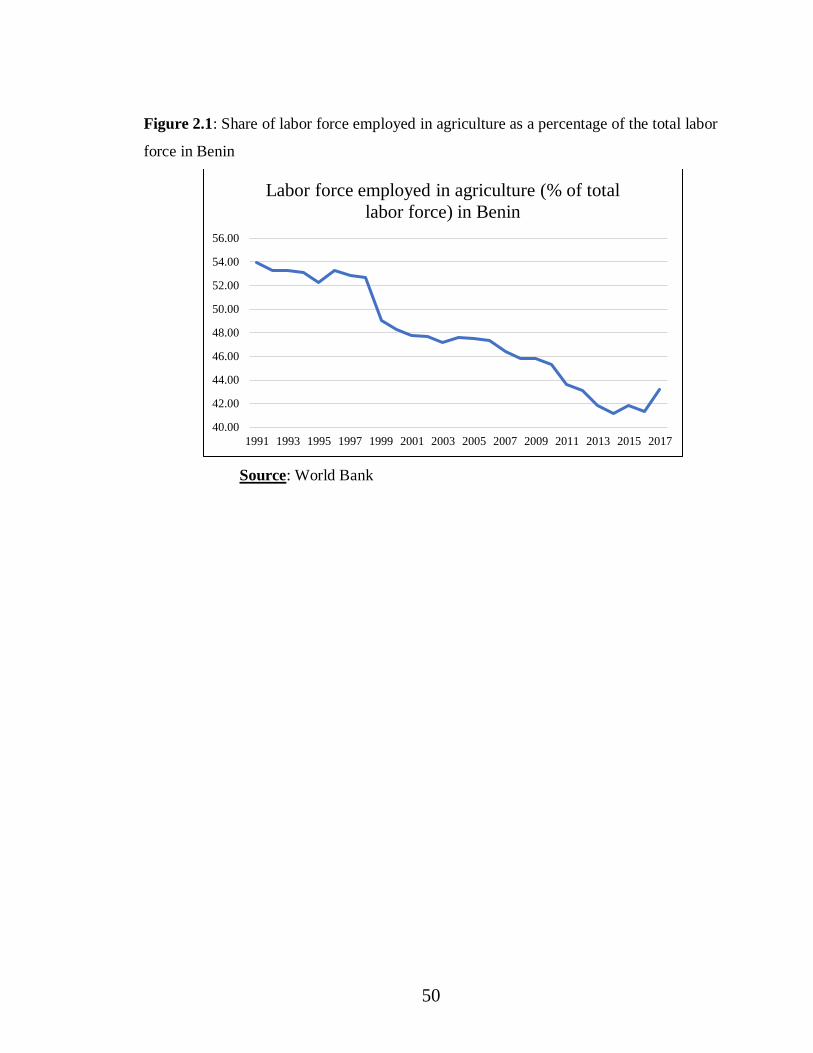
50

Figure 2.1: Share of labor force employed in agriculture as a percentage of the total labor

force in Benin

Source: World Bank

40.00

42.00

44.00

46.00

48.00

50.00

52.00

54.00

56.00

1991 1993 1995 1997 1999 2001 2003 2005 2007 2009 2011 2013 2015 2017

Labor force employed in agriculture (% of total

labor force) in Benin

51

3. Does experience with agricultural loans improve farmers’ efficiency in Benin? A

stochastic frontier analysis

3.1. Introduction

In Benin, as in most developing countries, the performance of the agricultural sector

plays a significant role in the overall economic growth and development. In 2014, the

agricultural sector contributed an average of 32.7% to the country’s gross domestic product

(GDP), and about 70% of the labor force was engaged in agriculture (MAEP, 2017).

Therefore, in Benin, agricultural growth plays an outsized role in reducing rural poverty

(Christiaensen, Demery, and Kuhl, 2011). Generally, the expected role of credit in the

agricultural sector is to relax farmers’ financial constraints and to increase their use of

productivity-increasing inputs. The expected impact of agricultural loans is, therefore, to

help farmers bring their input levels closer to the optimal levels, thereby increasing output

and productivity (Feder, Lau, Lin, and Luo, 1990). Because rural finance programs are

subsidized using limited taxpayer money, it is necessary to quantify their impact. If, on the

other hand, the marginal productivity of farm credit is minor, then resources may be better

used elsewhere.

This study evaluates the impact of agricultural loans on the whole-farm efficiency

of borrowers in Benin. First, a stochastic translog profit frontier model is estimated, and

farm efficiency scores are derived. Then, using a propensity-score matching technique, the

efficiency scores of experienced borrowers are compared to those of inexperienced ones,

providing a measure of the marginal effect of loan experience. In the context of this

research, whole-farm profit efficiency is the most appropriate measure of loan impact since

households tend to have multiple farming activities, and even a loan taken for a specific

activity will ease a household’s overall cash constraint.

An important policy concern in Benin, as in many countries in sub-Saharan Africa,

is how to raise agricultural production, given limited resources, to meet the growing

demand of a growing population. Future agricultural growth must rely more on raising

productivity rather than expanding resources. The potential importance of efficiency as a

way of fostering production has generated a substantial number of studies (Bravo-Ureta

and Pinheiro, 1993). Before further discussion, it is important to distinguish between

52

efficiency and productivity. Productivity growth can be achieved through technological

progress and/or efficiency improvements; with each implying a different set of policies

(Coelli, 1995). The efficiency of farmers and, more specifically, the efficiency gains from

experience with agricultural loans matter because such gains present a sustainable and

relatively low-cost way to achieve productivity growth. Measuring efficiency is the first

step to potential resource savings (Bravo-Ureta and Rieger, 1991). If farmers are thus found

to be reasonably efficient in their resource allocation, then the implication is that improving

productivity necessitates new technology and inputs, something that would require

investments in inputs provision, infrastructure, extension services and farm management

services (Mubarak Ali and Byerlee, 1991). Lastly, there are various measures of efficiency

in the literature. However, many of these are, by definition, partial measures (e.g., yield

and labor productivity). Analysing profit efficiency—a process that generates measures of

both technical and allocative efficiency—provides a more comprehensive view.

In contrast to most previous studies in the area, this study utilizes a comprehensive

definition of agricultural loans. Agricultural loans, here, refer to loans taken for all

agriculture- related activities, including crop production, animal husbandry, processing,

and trade and storage of agricultural commodities. Given the income-generating nature of

all of these activities, restricting the evaluation of the effect of credit to crop production

alone as a proxy for the rural world is a limiting approach. In the context of Benin, doing

so would also systematically exclude rural women, since it is typically women who carry

out these post-production activities.

The study estimates the effects of agricultural loans provided by one particular

micro-lender in Benin: Faîtière des Caisses d’Epargne et de Crédit Agricole Mutuel

(FECECAM). In its current form, FECECAM is a network of savings and credit

cooperatives with 136 service points throughout the country. It is, by far, the largest source

of agricultural loans in Benin. This analysis exploits differences in when clients took out

their first agricultural loan with FECECAM as the main source of identification of the

effects of FECECAM’s agricultural loans. The study relies on a “pipeline” design, or

cohort approach, in which subjects enter a program at different times. In this specific case,

the design allows the comparison of individuals with greater experience with credit to those

with little or none. The pipeline design represents a good alternative to a fully randomized

53

assignment because it offers a convincing control (Duvendack et al., 2011). Compared to

studies that use similar methods and even compared to most microcredit impact studies,

this research spans a larger impact timeframe (e.g., (Copestake, Bhalotra, and Johnson,

2001; Maldonado and González-Vega, 2008). To the best of my knowledge, this study is

the first of its kind to be carried out in Benin.

The remainder of this chapter is organized as follows: In the next section a conceptual

framework explains the notion of efficiency and its underlying theoretical foundation, as

well as laying down the hypothesized relationship between loans and efficiency. Then the

following section describes the profit frontier function and the process of using it to

estimate the average causal effect of FECECAM loans. Finally, the last section presents

and discusses the results.

3.2. Conceptual framework

3.2.1.The concept of efficiency: definition and measurement

The concept of efficiency is widely used in economics. It refers to the success of an

agent, herein a farmer, in producing the maximum possible output from a given set of

inputs (Farrell, 1957). Broadly, the notion of efficiency characterizes the utilization of

resources. In a sense, efficiency is a relative concept: it compares the performance of a

production unit to a standard.

Standard production theory, with its underlying concept of the production function,

provides the basic framework for the efficiency measures. The production function

represents the maximum amount of output attainable from a given input bundle with fixed

technology (Aigner, Lovell, and Schmidt, 1977). Similarly, a cost function gives the

minimum level of cost at which it is possible to produce some level of output, given input

prices. Finally, a profit function provides the maximum profit that can be attained, given

output price and input prices (Førsund, Lovell, and Schmidt, 1980). For each of the

functions presented, the concept of maximality or minimality is essential. The term frontier

can be meaningfully applied in each case because each function sets a limit to the range of

possible observations. A frontier denotes a bounding function (Coelli, 1995). The

pioneering work of Farrell (1957) led to the estimation of the so-called frontier production

functions, instead of the average production functions estimated previously. The

54

production possibility frontier provides the theoretical representation of the farm

production function and delimits the set of all possible outputs attainable for a level of input

sets and technology available (Schmidt, 1985). Hence, one may observe points below the

production (profit) frontier (farms producing less than the maximal possible output) or

points on the frontier (efficient farmers) but no points can lie above the production (profit)

frontier. The amount by which a farm lies below its production or profit frontier and the

amount by which it lies above its cost function can be used as a measure of its inefficiency.

The frontier function model of Farrell (1957) uses the efficient unit isoquant32 to

measure economic33 efficiency, and to decompose this measure into technical and

allocative efficiency (Bravo-Ureta and Pinheiro, 1993). In the frontier function model,

deviations from the frontier isoquant are associated with technical inefficiency and

deviations from the cost minimizing input ratios denote allocative inefficiency. Technical

efficiency (TE) indicates the farmer’s ability to produce the maximum output possible (the

frontier output) given a set of inputs and technology. Put differently, technical inefficiency

reflects the failure of attaining the highest possible level of output given inputs and

technology. Allocative (or price) efficiency (AE) measures the farmer’s success in

choosing the optimal input quantities that minimize costs, given the level of output and the

relative factor prices. Stated differently, allocative efficiency refers to the ability of the

farmer to use inputs in optimal proportions given their respective prices. Economic or total

efficiency measures the overall performance of the farmer and is equal to the product of

allocative and technical efficiencies. The choice of a specific measure of efficiency

depends on the objective.

Generally, there are two classes of frontier estimation methods: parametric and non-

parametric. Parametric frontiers rely on a specific functional form; they use econometric

techniques to estimate the pre-specified functional form and inefficiency is modeled as an

additional stochastic term. The stochastic frontier analysis proposed by Aigner et al. (1977)

is an example of parametric frontier approach. Non-parametric frontiers do not rely on a

32 The concept of frontier unit isoquant used by Farrell, (1957) evolved into the production and cost frontiers

of today (Kopp and Diewert, 1982). 33 Some of the paper’s terminology differs from what Farrell used in his work. For instance, Farrell used the

term price efficiency instead of allocative efficiency and the term overall efficiency instead of economic or

production efficiency. The terminology employed in this paper follows what has been often used in recent

literature.

55

specific functional form and use linear (or mathematic) programming. They were first used

by Farrell (1957) and reformulated as a mathematical programming problem by Charnes,

Cooper, and Rhodes (1978). Data envelopment analysis is the most commonly used non-

parametric approach. Frontier models can also be categorized into deterministic and

stochastic frontiers. In deterministic models, measurement errors or other sources of noise

are not taken into since the model assumes that any observed deviation from the estimated

frontier is due to inefficiency, while the stochastic approach allows for statistical noise

(Bravo-Ureta and Pinheiro, 1993; Coelli, 1995).

3.2.2.Agricultural loans and farmers’ efficiency

Despite the expansion of microloan programs, the literature lacks consensus regarding

the effectiveness of such programs. On one hand, studies show that microfinance does help

the poor improve their productivity as well as their well-being and enables them to pull out

of poverty (Girabi and Mwakaje, 2013; Otero, 1999; Pitt and Khandker, 1998). On the

other hand, other studies claim that evidence supporting the positive impact of

microfinance interventions is thin and lacking in rigor (Banerjee et al., 2014; Feder et al.,

1990; Roodman and Morduch, 2014).

Agriculture in developing countries has experienced profound changes in the face of a

rapid technological change. In a traditional agriculture, farmers mostly depend on their

own resources and have had a long period to adjust their management to the most efficient

use of their resources in their environment. However, in a dynamic setting, characterized

by a continually changing technical and economic environment, it is more difficult for

farmers to adjust their allocative decisions to keep up with changes in their environment

and, simultaneously maintain an efficient allocation of resources. Thus, in such context,

farmers are more likely to be in a state of continuous disequilibrium with potentials and

benefits in improving their information and skills to reduce their technical and allocative

errors (Ali and Byerlee, 1991).

Access to financial instruments closely influences farmers’ decision to invest and to

produce (Karlan, Osei, Osei-Akoto, and Udry, 2014). Microfinance services in general,

and microcredit specifically has a very important role to play in today’s technically-

dynamic agriculture that depends greatly, inter alia, on the use of purchased inputs, hired

56

labor, machinery services or financial services. In fact, when assessing the determinants of

farm level variation in efficiency, several studies conclude that access to credit has a

positive and statistically significant impact on farmers’ technical and allocative efficiency

(Ali, Parikh, and Shah, 1994; Bravo-Ureta and Pinheiro, 1993). For instance, five out of

eight studies in the review of Bravo-Ureta and Pinheiro, (1993) showed that credit has a

positive and significant effect on the efficiencies of the farmers. The current study

identifies different channels of influence of agricultural loans on farmers’ efficiency.

At the beginning of the production period, agricultural loans may augment farmers’

initial endowment to help them face lump sum productive investments. Given the

indivisible nature34 of some inputs needed, lump sum expenses are required. Cash

constraint could lead to a bad combination of inputs if the farmer is unable to purchase

those inputs at all, causing inefficiencies. Credit availability, therefore, allows constrained

farmers to make the optimal input mixes to produce efficiently (optimal input mix effect).

Given that production efficiency depends on input decisions, microfinance services,

and more specifically agricultural loans will increase borrower’s productive power by

fostering investment in farming activities and improving farmers’ access to inputs. More

specifically, agricultural loans will lead to the purchase of better performing or modern

inputs that may be costly but have higher returns. Even though these technologies may

increase the production cost, they often have economies of scale that lead to higher output

levels per production costs. Obviously, everything else equal, farmers with better inputs

access are expected to have higher efficiency levels compared to the constrained ones who

are more likely to underinvest in resources. Thus, agricultural loans will positively affect

farmers’ total efficiency. Production loans, by relaxing farmers’ budget constraint grants

them the opportunity to purchase and use technologies such as improved seeds, fertilizers,

pesticides, farm machinery, etc. Most of these technologies will increase farmers’ output,

profit, and productivity (scale effect).

However, one can argue that the mere provision of loans may help farmers operate at

a higher production frontier but might not necessarily make them more efficient. In this

study, the treatment variable considered is not the access to credit but the experience with

34 For example, farmers cannot purchase portions of a pesticide bottle because (s)he has a small farm.

57

the loans over a relatively extended period of time. If the simple provision of loans does

not help farmers improve their resource allocation, their experience with the loans over

time is more likely to help them learn the best practices, and this learning and experience

will ultimately help farmers adjust their technical and allocative decisions to reach an

equilibrium of efficiency. Farmers with more experience with loans are expected to be

more efficient as they learned over time how to choose the right proportions of inputs to

produce the most possible output not only to be profitable but also to be efficient.

Furthermore, most loan programs including FECEAM’s offer training as well as

educational support to their clients to help them improve their management as well as their

financial skills to better conduct their funded activities. In this case, it is reasonable to

expect such loan programs to have a positive impact on clients’ allocative efficiency

particularly. Recall, allocative efficiency is the ability to use optimal proportions of inputs.

Allocative inefficiencies are errors in the allocation of inputs within expenditure levels.

These inefficiencies, for the factors that depend on the farmers, are caused mostly by

inadequate information; other causes of allocative inefficiency include market failure in

input supply, differential risk effects of inputs, institutions (e.g., tenancy) (Ali and Byerlee,

1991). Borrowers with higher numbers of loans, which imply several pieces of training

from the MFI, are expected to have a higher (allocative) efficiency score

((learning/experience effect). More, credit users with frequent extension visits and a higher

educational level may have higher efficiency levels.

Finally, the examination of secondary data provided by FECECAM showed that some

farmers requested amount of loans that are smaller than the amounts they have in their

saving account(s). In other words, they could have invested their savings in their productive

activities but they prefer to take out loans. These borrowers argued that such behavior

“pushes them to work harder and produce better”. FECECAM staff members confirm this

explanation of such behavior arguing that, having the weight of a loan that needs to be

repaid, gives some borrowers a reason to “work harder” to have a successful production

season. Even though, this argument is anecdotal, one can argue that agricultural loans have

an incentivizing effect that pushes farmers to produce the highest possible output with their

resources. Farmers improve their production process to be able to make profit and repay

the loan including the interests.

58

3.3. Empirical framework

3.3.1.The profit frontier function

In the literature, technical and allocative inefficiencies have been widely studied in the

context of single-output technologies (Kumbhakar, 1996). This paper models these

inefficiencies in a multiple-output, multiple-input context. The sample agricultural

borrowers conduct several productive activities including multiple crops production,

animal raising, processing and trade of agricultural products. Overall, they conduct on

average 2.77 (1.21) distinct income generating activities including non-farm one. More

in detail, on average, sampled borrowers produce 1.84 (1.24) different crops, conduct 0.38

(0.64) distinct agricultural products processing and trade activities, and 13.90 %

(34.62%) raise animals. In such context, inputs can be assumed non-allocable, meaning

that one observes the total quantities of the different inputs used in the production process,

instead of the quantities of each inputs allocated to different outputs (Kumbhakar, 1996).

The production process is therefore represented by a single equation including all outputs

and inputs.

Typically, (economic) efficiency is analyzed by examining separately its two

components: technical and allocative efficiencies, and the conventional production

function approach suffices to measure these efficiencies. However, a production function

may not be appropriate when estimating the production efficiency of individual farms when

they face different input and output prices and have different factor endowments (Ali and

Flinn, 1989; Yotopoulos and Lau, 1979). In fact, in such case, farms have different best-

practice or frontier production functions and, thus, operate at different optimal points.

Consequently, a stochastic profit frontier function, which is more suitable, is applied to

directly estimate farm-specific efficiencies. This estimation process incorporates prices

differences, market distortions but maintains the advantage of the stochastic frontier

properties in efficiency analysis (Ali and Flinn, 1989; Wang, Cramer, and Wailes, 1996).

The profit frontier combines both measures of efficiency into one, the profit efficiency. In

this profit relationship, errors in the production decision translate into lower profits or

revenue for the farmers (Ali et al., 1994). In addition, deviation of actual profits from the

59

profit frontier function can be interpreted as the aggregated technical and allocative

inefficiency (Ali et al., 1994).

Scholars have also argued that socio-economic variables should be incorporated

directly in the frontier model because such variables may have direct impact on the

efficiency (Battese and Coelli, 1995; Kumbhakar, Ghosh, and McGuckin, 1991). Put

differently, the stochastic frontier model should be estimated as a function of explanatory

variables, reflecting farm-specific characteristics. This study integrates directly farm-

specific characteristics in the estimation of the stochastic profit frontier function.

The stochastic profit function is defined as followed:

𝜋𝑖 = 𝑓(𝑥𝑖; 𝛽)𝜀𝑖 (1)

where 𝜋𝑖 is the profit aggregated over all farming activities of the ith borrower and

calculated as the gross revenue less the variable costs. 𝑥𝑖 is a vector of input expenditures

(labor and other variable costs/capital) of the ith borrower and 𝛽 is the unknown parameters

to be estimated. The ith borrower makes profit using the technology 𝑓(𝑥𝑖; 𝛽). A borrower

make lower profit than predicted by the profit function when errors occur in the production

system, leading to inefficiencies denoted by 𝜀𝑖. The inefficiency term satisfies the condition

0 < 𝜀𝑖.< 1 and the closer 𝜀𝑖 is to 1, the more (profit) efficient the borrower is.

To estimate the stochastic profit frontier, the study assumes that the profit function

takes a translog35 form. The translog functional form offers a relative flexibility compared

to a Cobb-Douglas function. In fact, a translog profit function does not impose assumptions

about constant elasticities of production nor elasticities of substitution between inputs,

allowing the data to reveal the actual curvature of the function, rather than imposing a priori

assumptions. The translog profit frontier, illustrating a case of two inputs, is expressed as:

𝑙𝑜𝑔 𝜋𝑖 = 𝛽0 + 𝛽1𝑙𝑜𝑔𝑥1𝑖 + 𝛽2𝑙𝑜𝑔𝑥2𝑖 + 𝛽3𝑙𝑜𝑔𝑥1𝑖𝑙𝑜𝑔𝑥2𝑖 + 𝛽4𝑙𝑜𝑔𝑥1𝑖𝑙𝑜𝑔𝑥1𝑖 +

𝛽5𝑙𝑜𝑔𝑥2𝑖𝑙𝑜𝑔𝑥2𝑖 + 𝜀𝑖 (2)

Consistent with the frontier concept, the error term 𝜀𝑖 in the profit function is also a

compound disturbance term, which have a strictly nonnegative and symmetric distribution,

respectively.

𝜀𝑖 = 𝑢𝑖 + 𝑣𝑖

35 Several studies including Kopp and Smith (1980) indicated that functional specifications have little to no

impact on measured efficiency.

60

𝑣𝑖, which is the idiosyncratic component, is independently (iid) ~ 𝑁(0, 𝜎𝑣) distributed over

the observations and reflects random factors beyond the control of producers such as the

weather. 𝑢𝑖 is a one-sided disturbance term that represents the inefficiency component. It

is assumed to have a half-normal distribution (non-negative and absolute value of a normal

distribution).

Next, the profit inefficiency term is specified as a function of covariates 𝑍𝑗 including socio-

demographic as well as farm-specific characteristics such as borrowers’ education, contact

with extension service, etc.

𝑢𝑖 = 𝛼0 + ∑ 𝛼𝑗

𝑗

𝑍𝑗𝑖 + 𝜉𝑖

Both the profit frontier function and the inefficiency models are estimated jointly using

the maximum likelihood estimation method.

3.3.2.Estimating the effect of loan experience on borrowers’ efficiency

The ultimate goal of the study is to estimate the average causal effect of FECECAM

loans on the efficiency of its agricultural borrowers. Earlier, in section 1.5.3, the biggest

threat to identifying that causal effect has been addressed. The study exploits clients’

program entry timing along with their borrowing history with FECECAM to construct

reliable treatment and control groups using a clustering technique. The treatment

considered is the experience with FECECAM loans. The treated group represents

borrowers, to whom the MFI has been lending for an extended period. More specifically,

the treated group includes borrowers, who, on average, have joined FECECAM 15 years

prior to the study, have taken four times a loan and have received an average of 1,126,000

FCFA of loan each time. A total of 153 borrowers (20.45%) meet those conditions in the

sample. The control group consists of borrowers, who, on average, entered the loan

program only three years before the study, have obtained a loan two to three times, and

have received an average amount of 300,000 FCFA of loan each time they have borrowed.

79.55% of the sample falls into that category.

The K-means cluster analysis permits to create two groups within which observations

are very similar, but observations in different groups could also be dissimilar. In other

words, borrowers within the treatment or the control group share very similar

61

characteristics, however, as shown by the results from the t-test (table 1.4), experienced

borrowers could differ from inexperienced ones based on some observables features such

as age.

One way to bridge that gap between the treatment and the control group is to match

similar borrowers based on those factors of dissimilarity across groups, that actually are

not influenced by their experience with loans, but instead determine their likelihood to be

treated, here to be an experienced borrower. All these factors are “summarized” for each

subject in a so-called propensity score, in this case, the propensity to be an experienced

borrower. More specifically, the propensity scores are the conditional (predicted)

probabilities of receiving treatment given pre-treatment or baseline characteristics. The

study computed the propensity scores of the sampled borrowers using a logistic function.

𝑝(𝑥) = 𝑝𝑟𝑜𝑏(𝐷 = 1|𝑧) = 𝐸(𝐷|𝑧)

Where D is the dependent variable and take the values D = 0 for control

observations and D = 1 for treated observations; 𝑧 is a set of explanatory variables.

The covariates used to predict sampled borrowers’ probability to be treated are the

lender’s selection criteria along with other factors drawn from the literature. For instance,

the borrower’s age is an important criterion of selection for the cooperative and thus, a

significant predictor of treatment. To be eligible for a loan with FECECAM, applicants

must be 18 to 70 years old at most. Applicants must also have some experience conducting

income generating activities as well. Therefore, working young and middle-aged adults are

more likely to have some borrowing experience with FECECAM. Women are also

“trusted” because they tend to have a lower rate of default. For proximity matter,

FECECAM requires all its applicants to reside in the town or at least in the Commune36 in

which they are requesting a loan. Indicators of wealth and the ability to provide collaterals

also greatly affect the lender’s decision to provide a loan. Consequently, predicting

variables used are socio-demographic characteristics such as age, gender, educational level,

status in the household, work migration experiences as well as household structure

including household size, family workforce computed in adult equivalent37. The covariates

36 Communes are the second administrative territorial divisions in Benin after villages/cities and there are

seventy-seven (77) communes in Benin. 37 To estimate family workforce in adult equivalent (eqa), the age of each household member actually

working or helping on the production units of the household is multiplied by the following coefficients: 0.33

62

also comprise socio-economic features such as the number of income generating activities,

years of experience conducting farming activities, land available to the household,

household assets, farm and non-farm income, and the proximity to a FECECAM service

point as well as the location in an agricultural zone. Note that except for gender and

location, these variables are related to the age of the borrower.

In a next step, individuals from the treatment group, the experienced borrowers, are

matched to those in the control group that have similar level of propensity score. Given

that the number of borrowers in the control group is more than three times the number of

those in the treatment group, each experienced borrower is matched to three nearest

“neighbors” in the control group, i.e., the three nearest inexperienced borrowers with

similar propensity scores. Finally, treatment effects are calculated by comparing the

outcomes (efficiency levels) of matched observations. The causal effect of FECECAM

loan experience on the whole-farm efficiency of borrowers is assessed using two treatment

effects statistics: the Average Treatment Effect (ATE) and the Average Treatment Effect

on the Treated (ATET or ATT).

3.3.3. ATE versus ATET

The average treatment effect (ATE) measures the effect that a substantial experience

with FECECAM loans would have on the entire population or what would have happened,

had all borrowers been treated or experienced. To obtain the ATE, the potential outcome

(PO) of each subject in the sample is calculated first. The PO is the outcome that would be

observed if each sampled individual received a specific value of the treatment (the

counterfactual). For experienced borrowers, the PO if they were inexperienced is computed

while for the PO if experienced is estimated for borrowers in the control group. The ATE

is the average difference between the actual outcome and the potential outcome of each

subject.

The average treatment effect on the treated (ATET or ATT) estimates the effect of the

treatment on those who received it, in other words, how much the efficiency of the

eqa for a child from 6 to 10 years, 0.66 for a child from 11 to 15 years old, 1 for a person from 16 to 50 years

old, 0.66 from 51 to 65 years and 0 beyond. These are the FAO coefficients for adult equivalency in labor

force.

63

treatment group improved as a result of their experience with FECECAM loans. The ATET

is the difference between the outcome of the treated and the control groups.

The ATE and the ATET answer different economic policy questions, especially in

cases like this where participation is voluntary. The ATE estimates the effect of a policy or

program on the persons induced to change participation status by the policy/program. It

ignores the effect of the variation in policy parameter on inframarginal person (Heckman,

1997). Participation in FECECAM’s loan program is voluntary and one can argue that there

will always be individuals who will choose not to borrow from the institution. Instead of

considering the marginal effect of FECECAM loans for the entire population, the effects

of FECECAM loans in its current state, on those who choose to participate may be more

informative. For the German Development Institute who commissioned this investigation,

the ATET estimating the effects on those who actually choose to borrow is a better

indicator of the effect of loan on efficiency compared to the ATE expressing the effects of

loans in a hypothetical scenario where everyone in the population would borrow from

FECECAM. In the case of a required vaccine for instance, the ATE would be more

meaningful.

The ATET, however, can be criticized from different standpoints. In general, the

assumptions required to estimate the ATET are less restrictive and weaker than those

required to estimate the ATE. Thus, ATET could suffer from biases, especially in

observational studies if the treatment and the control groups are not similar. Though, it is

shown not to be case in this study (see section 1.5.3.). Typically, the ATET should38 give

the same results as a t-test between the outcomes of the treatment and the control groups.

3.4. Results

3.4.1.Data overview

Variables description

Table 3.1 presents a descriptive summary of the variable used in the analysis. The

sample includes 67.78% of male respondents, and the average age of all respondents is

about 43 years. The average credit user has three years of education, conducts three income

38 Unlike the ATE, the estimation of the ATET requires finding matches for treated subjects only. Thus, all

individuals in the control group may not be used.

64

generating activities, farm and non-farm included, and has been conducting those activities

for 19 years. Their households have an average of eight members, which is relatively large

compared to the country mean of 5.8739 recorded by Benin’s population census of 2013.

Likewise, the area of land available and owned by the households of the respondents is

high, 9.3 ha on average. Even the mean value of household durable goods or assets owned

by the respondents in 2017 during the survey indicates that the sample of borrowers does

not mainly include the traditional poor small farmers. The average value of the household

assets owned by the respondents is 2,000,000 FCFA.

Farming activities

The study considers all farm related activities funded by FECECAM. Specifically,

agricultural loans, in this analysis, refers to loans taken for agricultural related activities

including crop production, animal husbandry, processing, and, trade of agricultural

commodities. As shown earlier, farmers in Benin are engaged in multiple farming activities

that contribute to their income, thus to their farm profit. Each respondent weighted the

relative contribution of their various activities to their monetary income. The average

weight obtained represents an approximate value of the relative contribution of each type

of activity to the farmer’s income. The relative contribution of the activities are described

by region in figure 3.1.

Overall, in all studied regions, crop production remains the main source of income

for the sampled borrowers. It comprises more than 50% of their income. The contribution

of crop production to the respondent’s income increases from the South to the North. For

borrowers in the North, crop production comprises 82.2% of income. Maize is the main

crop produced (30.5% of income), followed by cotton (27.4%) and soybean (11.7%).

Concerning animal raising, cattle dominate. Agricultural products are marginally

processed but mainly used in local street food production in this region.

In the Center, even though crop production is the main source of income, trade of

agricultural products represents a sizeable portion of the recipients’ income. Trade in the

Center totalizes the highest contribution to income compare to the North and the South.

Processing activities remain moderate, but more important than in the North. Animal

39 Data made available by Benin Data Portal (2016).

65

husbandry contributes to 4.1% of recipients’ income in the region, and mostly through

livestock trade. Animal husbandry is more diversified compared to the North, and cattle

are dominant but followed by pigs.

While income structures in the North and Center do not differ fundamentally, it is

not the case in the South. The main source of income remains crop growing (57.0%) but

the leading crops are pepper (8.6%), maize (6%), cassava (6%), pineapple (5.6%), sweet

potato (4.9%) and tomato (4.8%). Farm produces are more often processed locally (10.5%),

with alcohol production at the top of a long list of processing activities (cassava in flour,

palm nuts in oil, cereals in various products, smoked fish, soy in milk and derivatives, etc.).

Animal raising is more important than in other regions (4.5%), and is dominated by poultry

and pigs.

Overall, agricultural borrowers in the North specialize mostly in crop production while

in the Center, production and trade dominate; and in the South, production and processing

are the farming main activities.

3.4.2.Stochastic profit frontier estimation

The first step is the estimation of a stochastic translog profit function, which represents

the best-practice technology against which the efficiency of the borrowing farmers can be

measured. The results are presented in table 3.2. Following Kumbhakar et al. (1991), the

specification includes direct estimation of determinants of profit efficiency along with the

parameters of the frontier model. To capture regional heterogeneity, the profit frontier is

estimated per studied region: the North, the Center and the South.

Prior to the profit frontier estimation, a likelihood ratio test of the presence of an

inefficiency component in the model is performed. The test’s null hypothesis is H0: 𝜎𝑢2 = 0

against the alternative hypothesis H1: 𝜎𝑢2 > 0. If the null hypothesis is true, then the

stochastic frontier model reduces to the classical Ordinary Least Square (OLS) model with

normal errors. In the specification combining all regions as well as in the specifications for

the North and the South, the null hypothesis is rejected, indicating that a significant part of

the variability in profits among agricultural borrowers is explained by existing differences

in efficiency levels. The estimation of a stochastic profit function is therefore justified.

However, in the Center, we fail to reject the null hypothesis.

66

Furthermore, the variance ratio parameter, λ = 𝜎𝑢/𝜎𝑣, proposed by Battese and

Corra (1977) is greater than 0 and relatively large (λ = 2.21 in the North, λ = 0.78 in the

Center, and λ = 1.65 in the South). This result implies that deviations from the maximum

profit among agricultural borrowers in the North and the South stemmed from differences

in producer practices rather than random variability (λ > 1). In the Center, however, λ is

different than zero but less than unity indicating that the idiosyncratic component

dominates in the determination of the error term. There is some inefficiency but the

differences in profit among borrowers in the Center is prominently caused by random

factors outside the farmers’ control.

The sum of all parameters of the profit frontier model is lower than unity

(∑ 𝛽𝑗 < 1𝑗 ) in all regions indicating that borrowers operates with diminishing returns to

scale technology. In the South, both the increase in labor and other variable inputs are

positively and significantly associated with increase in output and profit. Across all

regions, other variable inputs (capital) significantly and positively affect the profit.

Recall, labor cost includes the value of in-kind and cash payments to hired laborers.

A variable indicating whether respondents report no labor expenditure has been included

in the inefficiency model. The statistically insignificant coefficient on that variable in the

North and the Center implies that profit does not really change when no labor expense is

reported. In fact, one can consider hired labor in this case as an indicative of the size of the

farm operation in those two regions–descriptive statistics show that borrowers in those

areas use mostly family labor: respectively 93.85% and 92.12% in the North and the

Center. A Probit regression of labor expenditure report shows that small farmers with less

capital do not hire any labor in those regions. Conversely in the South, where borrowers

employ mostly paid labor, the coefficient on the variable indicating that respondents report

no labor expenditure is positive and statistically significant. This result denotes that in the

South, labor expenditure is a significant share of the total cost such that farmers who do

not pay for labor in kind or in cash have higher profits.

A dummy variable for whether the sampled borrower belongs to a family of native

or first comer in the area displays a positive and significant coefficient in the Center and in

the South. This variable has been included in the model essentially to capture land

resourcefulness. In the South and the Center where land resources are scarcer than the

67

North, it makes sense that natives who own more land see a significantly positive effect on

their profit efficiency. In the Center and the South, specialization seems to improve profit

efficiency–the coefficient on the number of activities is negative in both regions but

statistically significant in the South only.

Surprisingly, the joint estimation of the frontier model and the efficiency factors

indicates inconclusive results on the relation between efficiency and household size or

family labor force.

In the Center, gender significantly affects the efficiency of the borrowers. In fact,

ceteris paribus, female agricultural borrowers are more efficient than male ones. They

possess less assets than male borrowers do, but they utilize their resources more optimally.

This result is very interesting and has important policy implications. It confirms previous

studies’ finding and the belief in the development arena that, policies targeting (rural)

women tend to be more effective. Resources or more specifically, money placed in

women’s hand seems to have bigger effect, not only on the household as demonstrated

previously (e.g. Thomas (1990)), but also on the farm. Put differently, the result supports

the recommendation that development program should target women because they tend to

be more efficient in resources use.

Surprisingly, the number of years of education has a negative effect on efficiency

in most regions. The coefficient is only statistically significant in the South. This result can

be explained by the fact that, the more educated the borrowers are, the more they tend to

practice farming as their secondary activity and therefore, are less efficient at it. For

instance, several respondents in the sample are school teachers or civil servants living in

rural areas and conducting some farming activities for additional income. The negative

sign on the coefficient of the number of income generating activities, even though it is not

statistically significant, supports this explanation.

3.4.3. Profit efficiency scores

The stochastic profit function model permits to uncover efficiency scores of

agricultural borrowers. These efficiency score are summarized in table 3.3. Recall, the

closer the efficiency scores are to the unity the more efficient the farmer is. On average,

farmers’ efficiency level is about 41% in the North, 57% in the Center and 44% in the

68

South. In general, sampled borrowers display low levels of profit efficiency denoting that

their farm as a whole could be about twice as profitable as it is.

The survey data help to better understand the different mechanisms contributing to

the different levels of efficiency per region. In the South, the most urbanized part of the

country, as well as in the North, the region with the highest agricultural production,

borrowers invest substantially in mechanized production equipment as well as in

transportation means40. In the South for instance, where farmers practice a lot of

horticulture, loans are frequently used to acquire irrigation equipment; whereas in the

North, sampled borrowers invest in tractors and land preparation machines. These

technologies help farmers reach a certain level of efficiency in production by increasing

their output (technical efficiency) but the cost associated with the investment into these

technologies increase their cost of production (allocative inefficiency) in the short term

studied. Consequently, in the North and the South the profit efficiency scores are the

lowest. In the Center, the investment in agricultural machines is moderate but hired labor

is predominant. Labor costs are often lower expenditure compared to machines and

equipment making sampled farmers in the Center more cost efficient in the short-term

given the technology used, compared to those in the North and the South. This result

validates the previous result that differences in profit in the Center is mostly caused by

random factors.

3.4.4. Agricultural loans and efficiency

To assess the impact of agricultural loans on farmers’ efficiency, the study employs

a treatment-effects model. A treatment effect is the change in an outcome caused by a

subject, here the agricultural borrower that receives a treatment instead of another. Three

main conditions underlie the use of treatment-effects estimators–the conditional-

independence (CI) assumption, the overlap assumption and the independent and identically

distributed (i.i.d.) sampling assumption.

The CI assumption ensures that the potential outcomes are conditionally

independent of the treatment and that no unobservable variable affect both treatment

40 Results from the previous chapter (Chapter 2) demonstrates this statement.

69

assignment and the potential outcomes, after conditioning on the observed covariates 𝑧.

Stated simply, under the CI assumption, there is selection on observables. To ensure that

the CI assumption is met, the study chooses a set of covariates that jointly determine the

selection process and the efficiency level of the borrowers’ farm. Also, given the sampling

framework and the identification strategy, one can argue that there are no unobserved

confounders or if any, potentially the morality of the client or her trustworthiness, they are

highly correlated with the covariates included in the model. Finally, there is a high degree

of post-match balance across the covariates. In fact, the box plots of matched data depicted

in figure 3.2 (North), figure 3.3 (Center) and figure 3.4 (South) indicate covariate balance.

Kernel density plots using the matched data also suggest balance.

The overlap assumption requires that each individual have a positive probability of

receiving each treatment level. Rosenbaum and Rubin (1983) call the combination of the

CI and the overlap assumptions strong ignorability. To check whether the overlap

assumption is violated, the estimated densities of the probability of getting each treatment

level are plotted. Figures 3.5, 3.6 and 3.7 display the estimated densities of the predicted

probabilities that an unexperienced borrower is unexperienced and the density of the

predicted probabilities that an experienced borrower is unexperienced, respectively in the

North, the Center and the South. The graphs show that the two estimated densities have

most of their respective masses in areas in which they overlap each other, and in all cases,

neither plot display most of its probability mass near 0 or 1. There is no evidence, therefore,

that the overlap assumption is violated.

The propensity score matching estimator is subsequently implemented and the

propensity scores are modeled using a logistic model, incorporating covariates such as age,

age square, gender, status in the household, education level, household size, assets, income,

proximity to a FECECAM branch, number of income generating activities, land

availability, and migration experience. Treated borrowers are matched to three control

borrowers with the closest propensity scores due to the higher number of control subjects

(almost three-fold).

After matching treated and untreated borrowers based on their propensity scores,

i.e. their predicted probabilities to be treated, the average treatment effects and average

treatment effect on the treated estimates have been elicited.

70

The matching results are summarized in table 3.4. Profit efficiency scores derived

from models estimated per region are the outcome variable in the estimation of the ATE as

well as the ATET. Section 3.3.3. earlier discussed the relevance of each statistic estimated.

Even though the result table report both the ATE and the ATET, the latter is the most

relevant figure in the case of this study. Though, the ATE shows that experience with loan

clearly has the potential to significantly increase the whole-farm efficiency of borrowers

by 3%, 2% and 5% respectively for those located in the North, the Center, and the South.

The statistic of interest, the ATET gives mixed results. In the North, farmers with

extensive experience with loan–loan experience according to the study is detailed in section

1.5.3.–significantly improved their whole-farm efficiency by 3.5%. This number is very

similar to the ATE obtained in the region and also similar to the difference in means from

the t-test, even though that difference (4%) was not statistically significant. In the Center,

ATET has a negative sign and is statistically significant. This surprising result could be

due to the small number of treated subjects in that region (only 33 experienced borrowers

versus 181 control). In fact, in the Center, even though the overlap and CI assumptions are

met, the match balance or overlap degrees are still low. Also, the frontier estimation

showed that in the Center, differences in profit are predominantly caused by random factors

out of farmers’ control. In the South, the ATET is not statistically significant even though

it has a positive sign implying that loan experience may improve borrowers’ whole farm

efficiency.

It is noteworthy that the frontier estimation shows that sampled borrowers located

in the North and the South have the lowest profit efficiency scores whereas the matching

results reveal that borrowers located in those regions have the highest gain in efficiency

from loan experience.

Overall, judging by the ATET, matching results indicate that the use of agricultural

loans significantly increase the profit efficiency levels of experienced borrowers

particularly in the North. Even though the change in efficiency is small, it has some

important financial implications for the borrowers. In fact, these results put into perspective

mean that over the six-years period studied (2012-2017), borrowers who received on

71

average four times ( 1.77 times) an average amount of loan of 1,126,000 FCFA41 (

1,2630,000 FCFA) improved their whole-farm profit efficiency by 3.5% on average for

those located in the North. In that region where the mean farm profit for the 2016-2017

agricultural season is 2,062,000 FCFA ( 4,797,800 FCFA), the improvement in efficiency

represents a yearly gain in profit of 72,170 FCFA ( 167,923 FCFA). This gain is quite

significant in a country like Benin where 40.1% of the population live below the poverty

line (The World Bank, 2016).

The results of the study clearly indicate that FECECAM’s loans not only help

borrowers become better farmers but also improve their resource allocation.

3.5. Implications and Conclusion

The performance of the agricultural sector has a key role to play in the sustainable

economic development of African countries. Yet, intensification and modernization

typically require capital, which is not often available to farmers. The lack of capital

represents a significant constraint to the development of the agricultural sector. The goal

of this chapter is to gauge the effectiveness of agricultural credit programs as a policy tool

for increasing the income and the productivity of farmers. More specifically, the chapter

examines the effect of agricultural loans on input allocation decisions and farm

profitability. It evaluates the impact of agricultural loans on the whole-farm efficiency of

borrowers in Benin. The analysis exploits differences in loan take-up timing, frequency

and amount received as the source of identification of the effects of agricultural loans

provided by the largest microfinance instiution in Benin (FECECAM).

Using primary data on the clients of FECECAM, this chapter, first, estimates a

farm-level stochastic profit frontier. The results of the frontier analysis reveal, among other

things, that even though (or, perhaps, because) rural women own fewer assets than their

male counterparts, they are made more efficient by loans in their resource allocation. This

result supports the fact that development programs targeting women have bigger effect.

Next, the frontier function allows the estimation of borrowers’ profit efficiency

scores, which is an aggregate measure of technical and allocative efficiency. The estimated

41 About 2,000 USD

72

average profit efficiency is about 41% in the North, 57% in the Center and 44% in the

South, denoting the presence of significant technical and allocative errors leading to profit

loss in all studied regions. Sampled borrowers’ farm could be about twice as profitable as

it is. In light of the survey and the previous chapter, the chapter discusses the mechanisms

explaining the differences across regions in efficiency levels. Farmers located in North and

the South have the lowest average efficiency scores due to higher costs of production (take

loan for machines and equipment purchase) while borrowers in the Center are able to keep

their production cost low by using hired labor. In all regions, FECECAM loans help

borrowers obtain inputs and technology they need to increase their production.

Then, propensity score matching technique helps compare the efficiency scores of

experienced borrowers to inexperienced ones, providing a measure of the marginal effect

of loan experience. The ATE shows that experience with loan clearly has the potential to

significantly increase the whole-farm efficiency of borrowers by 3%, 2% and 5%

respectively for those located in the North, the Center, and the South. The two regions with

the lowest efficiency scores have the highest (potential) gain in profit efficiency.

Considering the sampled farmers who are actually treated, experience with loan

significantly increase their efficiency particularly in the North, leading to a yearly gain in

profit of about 72,170 FCFA.

These results have important policy implications. First, results suggest that there

are significant inefficiencies in the way farmers allocate resources to their farming

activities. Furthermore, the use of agricultural loans in Benin clearly helps farmers improve

their productivity and profitability. The study provides a proof of the effectiveness of

agricultural credit programs and shows that agricultural loans have the potential to improve

farmer’s livelihoods.

73

Chapter 3 Tables and figures

Table 3.1: Summary statistics by region

(North) (Center) (South)

Variable Mean Std. Dev. Mean Std. Dev Mean Std. Dev

Farm production variables

Farm profit (100,000 FCFA) 20.622 47.978 43.957 143.848 33.084 103.925

Labor a cost (100,000 FCFA) 1.197 2.048 1.577 3.015 2.868 6.071

Other variable input cost (100,000 FCFA) 7.481 9.938 7.237 40.580 9.518 27.603

Other variables

Age (years) 42.848 11.513 41.530 11.697 46.214 10.111

Gender (Female =0; Male=1) 0.725 0.447 0.594 0.492 0.715 0.452

Household head (Yes=1; No=0) 0.674 0.470 0.629 0.484 0.757 0.430

Belong to a family of native or first comers in the area (Yes=1;

No=0) 0.674 0.470 0.522 0.501 0.456 0.499

Experience in conducting farm activities (Years) 17.063 11.158 17.164 10.617 22.622 11.007

Years of schooling (Years) 1.887 3.492 2.924 4.308 5.430 6.132

Length of (work) migration (Months) 5.934 24.117 12.769 42.490 11.561 32.754

Household size (Count) 9.354 4.897 7.809 3.940 7.004 2.999

Workforce available in the household (Adult equivalent) 3.387 2.236 2.910 1.612 2.506 1.423

Number of income generating activities (Count) 3.191 1.325 2.667 1.131 2.435 1.034

Land available to the household (Ha) 12.765 13.703 9.151 11.892 5.784 21.821

Value of household durable goods owned (100,000 FCFA) 7.291 24.092 16.015 50.947 38.000 69.610

Non-farm income in 2016-2017 (100,000 FCFA) 1.178 2.925 2.815 10.890 4.220 16.994

Number of extension visits received (Count) 0.922 2.029 0.784 2.599 0.644 3.770

Average loan taken between 2012 and 2017 (100,000 FCFA) 659.572 707.855 813.147 773.218 438.235 421.173

Cost one-way trip to closest FECEAM branch (FCFA) 20.622 47.978 43.957 143.848 33.084 103.925 a Labor cost includes the value of in-kind and cash payments to aids and workers for tasks undertaken during crop production,

processing and trade of agricultural products, and animal raising.

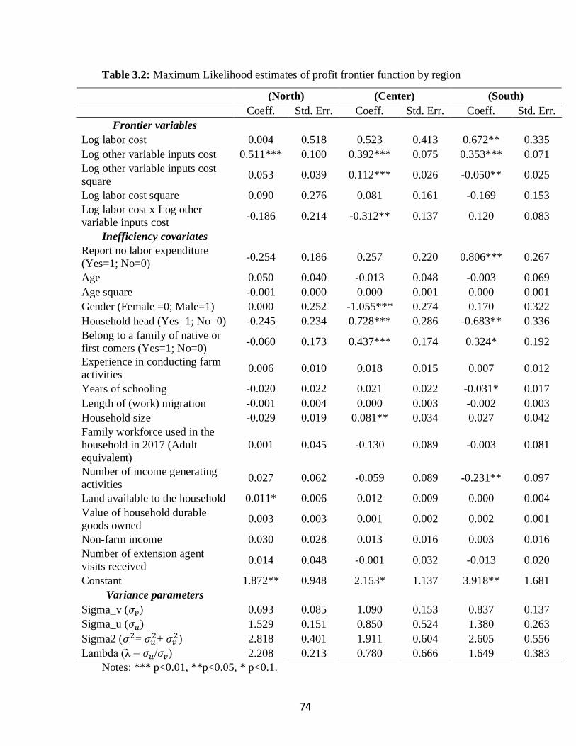
74

Table 3.2: Maximum Likelihood estimates of profit frontier function by region

(North) (Center) (South) Coeff. Std. Err. Coeff. Std. Err. Coeff. Std. Err.

Frontier variables

Log labor cost 0.004 0.518 0.523 0.413 0.672** 0.335

Log other variable inputs cost 0.511*** 0.100 0.392*** 0.075 0.353*** 0.071

Log other variable inputs cost

square 0.053 0.039 0.112*** 0.026 -0.050** 0.025

Log labor cost square 0.090 0.276 0.081 0.161 -0.169 0.153

Log labor cost x Log other

variable inputs cost -0.186 0.214 -0.312** 0.137 0.120 0.083

Inefficiency covariates

Report no labor expenditure

(Yes=1; No=0) -0.254 0.186 0.257 0.220 0.806*** 0.267

Age 0.050 0.040 -0.013 0.048 -0.003 0.069

Age square -0.001 0.000 0.000 0.001 0.000 0.001

Gender (Female =0; Male=1) 0.000 0.252 -1.055*** 0.274 0.170 0.322

Household head (Yes=1; No=0) -0.245 0.234 0.728*** 0.286 -0.683** 0.336

Belong to a family of native or

first comers (Yes=1; No=0) -0.060 0.173 0.437*** 0.174 0.324* 0.192

Experience in conducting farm

activities 0.006 0.010 0.018 0.015 0.007 0.012

Years of schooling -0.020 0.022 0.021 0.022 -0.031* 0.017

Length of (work) migration -0.001 0.004 0.000 0.003 -0.002 0.003

Household size -0.029 0.019 0.081** 0.034 0.027 0.042

Family workforce used in the

household in 2017 (Adult

equivalent)

0.001 0.045 -0.130 0.089 -0.003 0.081

Number of income generating

activities 0.027 0.062 -0.059 0.089 -0.231** 0.097

Land available to the household 0.011* 0.006 0.012 0.009 0.000 0.004

Value of household durable

goods owned 0.003 0.003 0.001 0.002 0.002 0.001

Non-farm income 0.030 0.028 0.013 0.016 0.003 0.016

Number of extension agent

visits received 0.014 0.048 -0.001 0.032 -0.013 0.020

Constant 1.872** 0.948 2.153* 1.137 3.918** 1.681

Variance parameters

Sigma_v (𝜎𝑣) 0.693 0.085 1.090 0.153 0.837 0.137

Sigma_u (𝜎𝑢) 1.529 0.151 0.850 0.524 1.380 0.263

Sigma2 (𝜎2= 𝜎𝑢2+ 𝜎𝑣

2) 2.818 0.401 1.911 0.604 2.605 0.556

Lambda (λ = 𝜎𝑢/𝜎𝑣) 2.208 0.213 0.780 0.666 1.649 0.383

Notes: *** p<0.01, **p<0.05, * p<0.1.

75

Table 3.3: Efficiency scores and mean comparison by region

All Experienced

(N=145)

Inexperienced

(N=529) Difference

Mean Std. Err. Mean Std. Err. Mean Std. Err Mean Std. Err

North

(N=220) 0.414 0.013 0.445 0.029 0.405 0.014 0.040 0.031

Center

(N=214) 0.568 0.007 0.597 0.016 0.562 0.007 0.035* 0.018

South

(N=181) 0.436 0.013 0.457 0.021 0.428 0.016 0.029 0.030

Notes: *** p<0.01, **p<0.05, * p<0.1.

Table 3.4: Treatment effect estimates by region

Region ATE ATET

Coefficient AI42 Robust

Standard Errors Coefficient

AI Robust

Standard Errors

North 0.030*** 0.003 0.035*** 0.006

Center 0.023*** 0.001 -0.023*** 0.004

South 0.048*** 0.004 0.007 0.008

Notes: *** p<0.01, **p<0.05, * p<0.1.

42 Stands for Abadie-Imbens robust standard errors

76

Figure 3.1: Contribution of farming activities to farmers’ income


matched data in the North

- ATE estimation

- ATET estimation

0% 10% 20% 30% 40% 50% 60% 70% 80% 90% 100%

North-East

Center

South

Contribution of activities to income

Crop production Trade of agricultural products Agricultural products processing

Animal raising and trade Wood crafts Non-agricultural products trade

Transportation activities Salaries Crafts and services

02

46

0 .5 1 0 .5 1

Raw Matched

control treated

Density

Propensity Score

Balance plot

0.2

.4.6

.81

Raw Matched

control treated

Pro

pensi

ty S

core

Balance plot

Pro

pensity s

core

0

.2.4

.6.8

1

Raw Matched

control treated

Pro

pensity S

core

Balance plot

Pro

pensity s

core

02

46

0 .5 1 0 .5 1

Raw Matched

control treated

Density

Propensity Score

Balance plot

77


matched data in the Center

- ATE estimation

- ATET estimation

0.2

.4.6

.81

Raw Matched

control treated

Pro

pensity S

core

Balance plot

Pro

pensity s

core

010

20

30

0 .5 1 0 .5 1

Raw Matched

control treated

Density

Propensity Score

Balance plot

05

10

15

0 .5 1 0 .5 1

Raw Matched

control treated

Density

Propensity Score

Balance plot

0.2

.4.6

.81

Raw Matched

control treated

Pro

pensity S

core

Balance plot

Pro

pensity s

core

78


matched data in the South

- ATE estimation

- ATET estimation

01

23

4

0 .5 1 0 .5 1

Raw Matched

control treated

Density

Propensity Score

Balance plot

0.2

.4.6

.81

Raw Matched

control treated

Pro

pensity S

core

Balance plot

Pro

pensity s

core

01

23

4

0 .5 1 0 .5 1

Raw Matched

control treated

Density

Propensity Score

Balance plot

0.2

.4.6

.81

Raw Matched

control treated

Pro

pensity S

core

Balance plot

Pro

pensity s

core

79

Figure 3.5: Estimated densities of predicted probabilities of getting each treatment level

in the North (overlap check)


the Center (overlap check)

80


the South (overlap check)

81

4. Impact of agricultural loans on farmers’ well being

4.1. Introduction

Given the importance of the agricultural sector in developing countries in general and

in Africa in particular, the sustainable economic development in these countries are

conditioned by the development of their agricultural sector. Limited access to financial

services is known as a major constraint to agricultural development (FAO, 2002). Farmers

need liquidity to face agricultural expenses throughout the production cycle but mainly at

the beginning. Production, as well as investment decisions of most farmers, are greatly

influenced by their access to financial instruments.

Mainstream financial institutions are reluctant to serve the agricultural sector for

several reasons. First, they consider the sector to be highly risky with a low performance.

In addition, agricultural activities depend on the weather, they take place in remote rural

areas, and commodities prices are volatile. All these aspects make it hard for standard

banks to reach their profit goals when lending to farmers.

Microfinance was initiated with the belief that access to credit has the potential to

transform the lives of those living in poverty (Grameen Foundation, 2016; Village Invest,

2016). In fact, microfinance, and more specifically microcredit has a dual mission:

financial inclusion and poverty alleviation. In the past 20 years, the microfinance sector

has experienced a rapid expansion, and the number of low-income households worldwide

with a microloan has considerably grown. From 1997 to 2010, an eighteen-fold growth is

recorded with an increase from 7.6 million to 137.5 million low-income families that

received a microloan (MSC, 2012).

However, evidence of the effectiveness of microfinance is still unclear. The literature

shows discrepancies between what microcredit ought to do theoretically and empirical

evidence. For instance, evidence from Cambodia suggest that microcredit may be most

appropriately conceptualized as a coping strategy instead of a poverty alleviation one

because borrowers perceive loans as useful in coping with household vulnerability, but not

transforming it (Bylander, 2015). In fact, microcredit opponents often argue that borrowers

would use microloans for consumption instead of investment in profitable activities,

resulting in repayment default, debt, and ultimately worsening the conditions of the

borrowers. More, farmers in developing countries face significant risk constraints along

82

with capital constraints. If lack of access to credit can limit farmers’ investment in activities

with higher profits, lack of access to formal insurance market can also prevent farmers

from investing in activities that may be risky, but have high expected returns (Cai, Chen,

Fang, and Zhou, 2015; Karlan, Osei, Osei-Akoto, and Udry, 2014). Furthermore, if the

funding of the agricultural sector must come from both the private and public sectors, it is

essential to demonstrate its value empirically, and provide reliable figures on the impact of

microfinance programs on agricultural clients’ living standards. Only, past studies on the

impact of credit suggest opposing results. On the one hand, studies show that microfinance

does help the poor improve their productivity or their well-being and enables them to pull

out of poverty (Girabi and Mwakaje, 2013; Pitt and Khandker, 1998). On the other hand,

other studies claim that evidence supporting the positive impact of microfinance

interventions are thin and lack rigor (Banerjee, Duflo, Glennerster, and Kinnan, 2014;

Roodman and Morduch, 2014).

The goal of this chapter of the dissertation is to assess whether agricultural loans work

as expected. The section estimates the impact of agricultural loans provided by the largest

microloan provider in Benin on farmers’ wellbeing. It tests the hypothesis that experience

with microcredit improves the well-being of the borrowers.

A simple model is developed to demonstrate how the allocation of agricultural loans to

the different needs of the recipient is a key determinant of how microloans affect the

livelihoods of their users. The model argues that to uncover an effect from microcredit,

loans have to be used for their purposes and suitable variables related to those purposes

need to be measured. It is possible that several studies which found no or negative impact

from microcredit use may have either missed the loan repurposing aspect, chosen the

wrong outcome variables or may have actually measured the effect of a “misuse” of loans.

The study employs four variables to gauge borrower’s well-being. The average impact

of loan experience is estimated on borrowers’ net farm income gained during the

agricultural season 2016-17. Net farm income is calculated as the sum of all revenues from

farm activities and farm-related services less cash and non-cash expenses. In addition, the

impact of FECECAM farm loans on recipients’ nutritional and food security status is

estimated. Borrowers nutritional status is measured using the Food Consumption Score

(FCS) and their food security status is assessed by the Food Insecurity Experience Scale

83

(FIES). Finally, the study takes a look at the specific impact of agricultural loans on rural

women using the composite and multidimensional indicator WEAI–women’s

empowerment in agriculture index.

Overall, the analysis shows that farm loans provided by FECECAM has a positive and

significant impact on borrower’s well-being. Female borrowers experience higher positive

impact of the loans compared to male.

4.2. Theoretical framework

4.2.1.MFIs’ strategy and expected impact of microcredit

When providing microloans, the strategy used by an MFI might greatly affect users’

perception of the loans and even the outcomes. Several studies, in fact, showed that

borrowers sometimes perceive loans from governmental institutions or development

programs as gifts and therefore fail to repay. For instance, studies by Houngan, (2015) and

Mazumder and Lu, (2015) indicated respectively in Benin and in Bangladesh that,

microcredit effects are consistently higher among non-governmental recipients compared

to governmental programs. FECECAM is a cooperative established since 1977, which has

substantial experience in credit disbursement. Over time, the lender has improved and

adjusted its loan programs’ implementation. FECECAM offers loans for specific purposes

and has a strict monitoring mechanism to ensure that borrowers use loans for their stated

purposes. After a thorough screening process for selection, the MFI ensures that borrowers

are actually using the loan for the initial activities through multiple site visits. These actions

ensure the selection of “good borrowers”, the good use of the loan provided but are also

deployed to guarantee a high repayment rate and the success of the programs.

Furthermore, a mandatory business management class is offered to all borrowers after

they are approved for a loan. Some branches offer technical assistance to the borrowers

depending on their activities, especially to women’s lending groups. During the loan

application, the farmer and the credit agent make a farm business plan as well as a home

plan for the coming agricultural season. As discussed earlier in the dissertation, these

practices make FECECAM loan programs very similar to supervised credit programs.

Farmers are provided loans but are also overseen and supported throughout the process. In

those conditions, one can expect an extended use of agricultural loans from FECECAM to

84

have the expected outcomes on the users’ socio-economic conditions. These empirical

observations lay the foundation for a discussion on loans expected impact.

4.2.2. Microloan allocation as determinant of its impact

Let’s consider a farm borrower who manages his economic activities within a farm

household. In general, farmers are concerned about production as they are about

consumption. An agricultural loan, even though received for a specific purpose, still

represents an increase in borrowers’ total cash, given that money is fungible. Thus,

agricultural loans temporarily relax recipients’ budget constraint. Suppose the borrower is

faced with only two choices. He/she can either use the loan for increasing productivity or

use it for consumption smoothing43. How the loan is allocated to his/her needs, as a result,

is a function of the farmer’s most pressing needs. In fact, loans provide our agent with the

facility to absorb random shocks in his income, and therefore prevent these shocks from

being transmitted into variations in consumption. Consequently, borrowers with more

assets are more likely to use their loan for increasing productivity as they will first use their

assets to cushion random income shocks while those with fewer assets are prone to

repurpose their loans towards consumption smoothing. In other words, we expect

borrowers with higher ability to pool risks across time to spend their loans towards

production instead of consumption smoothing. The central assumption here is that

agricultural loans have a positive impact or increase long-term productivity when they are

actually used towards their stated purpose, holding everything else constant (markets

access, extension services, weather, skills, and other factors). Accordingly, if agricultural

loans are working as expected, one should not expect an immediate short-term increase in

consumption, but rather a sustained increase in production which will eventually entail a

sustained increased consumption afterward.

Moreover, if agricultural loans, which are offered for increasing productivity, are

used instead for patching consumption, one can argue that borrowers become less likely to

produce the additional output needed to cover the additional charges represented by the

43 For simplicity, production here includes both the direct use of loans for inputs purchase as well as

productive investments. Also, we ignore the case where loans could be given or shared with friends or

relatives.

85

interest rate and the initial loan to be repaid. Consequently, if agricultural loans do not lead

to increased production, the repayment aspect of the loans become very burdensome for

borrowers who might even avoid taking loans for that reason. It follows that, ceteris

paribus, if agricultural loans are used for consumption smoothing, one can expect a higher

default risk.

4.2.3. Conceptual role of agricultural credit

At the individual level, an agricultural loan is expected lead to an immediate

increase in the use of inputs (land, capital, labor) toward agricultural activities or more

specifically toward the activity for which the loan had been taken. Given that certain inputs

such as fertilizers or new machines benefit various operations within the farm household,

one can expect a positive impact on borrower’s net farm income. Following a classical

production theory, a logical hypothesis is that an agricultural loan relaxes the budget

constraint facing the farmers and allows them to efficiently allocate factors of production

to maximize their profit. Overall, the anticipated pathway of the effects of FECECAM

loans at the individual level is the following. Agricultural loans allocated toward increasing

productivity is likely to stimulate a growth in the activity for which the loan is taken. The

income from this activity is prone to affect other activities of the borrower (growth,

substitution) and in total, these changes over time affect the accumulation of capital,

knowledge, technologies, economic and social links, and thus the borrower’s total income

(farm and non-farm). This income will be partly allocated to productive investments and

in the long-term to household durable goods acquisition. Hence, for variables such as farm

size, labor use44, productive assets accumulation, inputs expenses per farm area (hectare),

and net farm income, our model predicts an immediate sustained increase.

Furthermore, most microfinance programs target women with the goal to empower

them. The idea of promoting women’s empowerment by the provision of credit is not only

based on the assumption that women’s involvement in economic activities will strengthen

their social and political position, but also on the evidence that credit to women has a

positive impact on child welfare, girls’ schooling and food security. Our model also permits

44 The case of labor use will be discussed in detail in chapter 4.

86

predictions of the effects of microloans on women’s empowerment. In this study, the

definition of empowerment follows Kabeer (1999). One can argue that the women’s

empowerment in agriculture index employed in the study is a good composite and

multidimensional index to assess whether agricultural loans are actually increasing long-

term productivity in the special case of women in agriculture. In fact, the index takes into

account five main aspects of rural women’s constraints: (i) autonomy in decision-making

about their income generating activities; (ii) right over productive or household durable

goods including their holding; (iii) autonomy in the decision to take out loans; (iv) public

speaking and groups membership; and (v) the use of their time. For women who have

borrowed for an extended period of time, agricultural loans should help them gain more

autonomy and empowerment.

Finally, the model predicts an increase in consumption in the long run, subsequent

to an income rise, as a result of agricultural effectively increasing long-term productivity.

Indicators of household’s food security and food quality are employed to test that

assumption. Those who have borrowed for a longer period of time should display better

figures of food security and food quality indexes.

4.3. Impact estimation

The objective of this chapter is to estimate the average causal effect of FECECAM

loans on various indicators of borrowers’ well-being. Sections 1.5.2 and 1.5.3 respectively

discuss threats to identifying causal effects in microcredit studies and how the research

design and identification strategy addressed these threats. The research samples

FECECAM agricultural loan users only and exploits the timing of their entry into the

program along with their borrowing history with the MFI to construct reliable treatment

and control groups using a clustering technique. The loan treatment here is the experience

with FECECAM loans as defined in section 1.5.3.

To estimate the effect of loan experience on farmers’ well-being, the study uses a

treatment-effects model. Four indicators serve to measure the well-being of borrowers: the

net farm income, the Food Insecurity Experience Scale (FIES), the Food Consumption

Score (FCS), and the Women’s Empowerment in Agriculture Index (WEAI).

87

Outcomes of treatment and control groups are compared using a propensity score

matching technique, providing a measure of the marginal effect of loan experience. The

propensity scores are computed using a logistic model. Given the ratio between

experienced and inexperienced borrowers, each subject in a treatment group is matched to

two borrowers with the closest propensity scores in the opposite group.

The propensity score matching procedure is detailed in the previous chapter (see

section 3.4.4). Figures 4.2-4.5 depict the box plots of match data as well as Kernel density

plots using the matched data. Both graphs indicate in each case, a high or at least a

satisfactory degree of post-match balance (the conditional independence assumption is

met). Figures 4.6 to 4.9 display the estimated densities of the predicted probabilities that

an unexperienced borrower is unexperienced and the density of the predicted probabilities

that an experienced borrower is unexperienced, respectively in the case of the net farm

income, the FIES, the FCS, and the WEAI specifications. The figures show that the overlap

assumption is also met in all cases.

In general, borrowers in the treatment group are matched to those in the control

group based on selection criteria used by the lender as well as other factors drawn from the

literature and relevant to each specific indicator studied. These covariates include age,

gender, education, status in the farm household, work migration experiences as well as

household structure including household size, workforce available in the household in adult

equivalent. The covariates also involve characteristics such as the number of income

generating activities, the years of experience conducting farming activities, proximity to a

FECECAM service point as well as the location in an agricultural zone. Two treatment

effects statistics are estimated:

- The average treatment effect (ATE) measures the effect that a substantial experience

with FECECAM loans would have had on the entire population of borrowers or what

would have happened, had all borrowers been experienced ones.

- The average treatment effect on the treated (ATET or ATT) estimates the effect of the

treatment on those who received it, put differently, how much the well-being of the

treatment group improved as a result of their experience with FECECAM loans.

The previous chapter discusses the two statistics (see section 3.3.3) and argue that instead

of using the marginal effect of FECECAM loans on the entire population (ATE), the effects

88

of FECECAM loans in its current state, on those who actually chose to participate (ATET)

may be more informative. For the German Development Institute who commissioned this

investigation, the ATET estimating the effects on those who actually choose to borrow is

a better indicator of the effect of loan on efficiency compared to the ATE expressing the

effects of loans in a hypothetical scenario where everyone in the population would borrow

from FECECAM. In the case of a required vaccine for instance, the ATE would be more

meaningful.

4.4. Results

4.4.1. Loan repurposing and loan sharing

As mentioned earlier, FECECAM has tailored its agricultural loans to meet the need

of its clients. These farm loans are offered for specific purposes and the lender develops a

firm monitoring mechanism to ensure that clients are implementing the stated initial

purpose of the loan. Figure 4.1. displays the percentage of respondents who used their loans

for reasons different than the one stated in their loan application.

Overall, 23.4% of the loans received in 2017 were not used solely for the activity

for which they were requested. Most “changes in the purpose” are in fact an extension of

the use of the loans to more diversified agricultural or trade activities while some cases are

due to health expenses, and others are diversions in the strict sense of the term. The practice

of using a loan for extended agricultural activities is more frequent in the North (33.2% of

the respondents) where loans taken for cotton for example will be used to finance all or

other crops production.

With regard to diversion from the initial object of the loan, 4% of the recipients

shared their loan with others by becoming "resellers" (lenders) of money or promoters of

young farmers’ groups. Some recipients say that when other people who borrow from them

know that they also got a loan to fund them, they are more inclined to reimburse. Finally,

some respondents took agricultural credit but used it to pay their children school fees and

then paid back with revenues from their farming activities.

Surprisingly, loan sharing among household members is less common: only 4.1%

of male and 4.3% of female respondents did it. The perception that women are forced to

share their loans with their spouses is therefore not entirely valid, at least in Benin case.

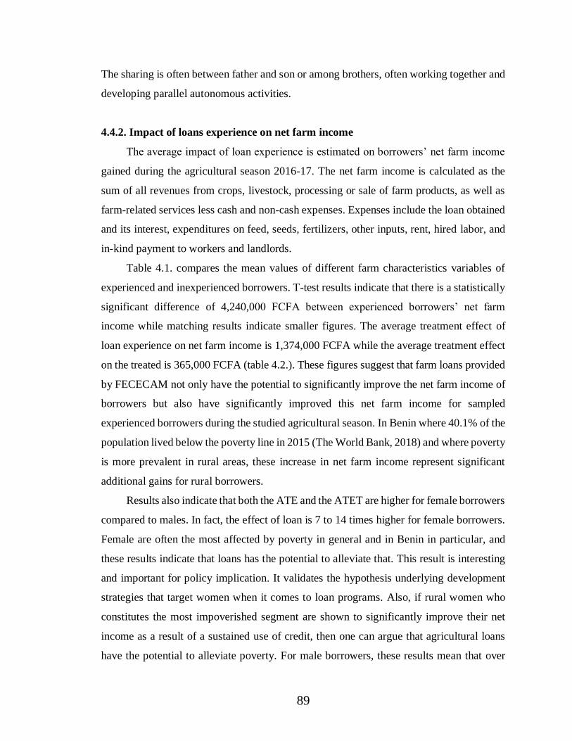
89

The sharing is often between father and son or among brothers, often working together and

developing parallel autonomous activities.

4.4.2. Impact of loans experience on net farm income

The average impact of loan experience is estimated on borrowers’ net farm income

gained during the agricultural season 2016-17. The net farm income is calculated as the

sum of all revenues from crops, livestock, processing or sale of farm products, as well as

farm-related services less cash and non-cash expenses. Expenses include the loan obtained

and its interest, expenditures on feed, seeds, fertilizers, other inputs, rent, hired labor, and

in-kind payment to workers and landlords.

Table 4.1. compares the mean values of different farm characteristics variables of

experienced and inexperienced borrowers. T-test results indicate that there is a statistically

significant difference of 4,240,000 FCFA between experienced borrowers’ net farm

income while matching results indicate smaller figures. The average treatment effect of

loan experience on net farm income is 1,374,000 FCFA while the average treatment effect

on the treated is 365,000 FCFA (table 4.2.). These figures suggest that farm loans provided

by FECECAM not only have the potential to significantly improve the net farm income of

borrowers but also have significantly improved this net farm income for sampled

experienced borrowers during the studied agricultural season. In Benin where 40.1% of the

population lived below the poverty line in 2015 (The World Bank, 2018) and where poverty

is more prevalent in rural areas, these increase in net farm income represent significant

additional gains for rural borrowers.

Results also indicate that both the ATE and the ATET are higher for female borrowers

compared to males. In fact, the effect of loan is 7 to 14 times higher for female borrowers.

Female are often the most affected by poverty in general and in Benin in particular, and

these results indicate that loans has the potential to alleviate that. This result is interesting

and important for policy implication. It validates the hypothesis underlying development

strategies that target women when it comes to loan programs. Also, if rural women who

constitutes the most impoverished segment are shown to significantly improve their net

income as a result of a sustained use of credit, then one can argue that agricultural loans

have the potential to alleviate poverty. For male borrowers, these results mean that over

90

the six-years period studied (2012-2017), receiving on average four times ( 1.77 times)

an average amount of loan of 1,126,000 FCFA45 ( 1,2630,000 FCFA) caused an increase

of 386,000 FCFA in their net farm income after the loan is repaid with its interest while for

female borrowers, this increase is nearly ten times higher (3,172,000 FCFA).

By disaggregating the results per activity group such as crop production, livestock,

processing and trade of farm products, results show a negative coefficient for female

borrowers for crop denoting that with improved income, female tend to move away from

growing crops and move toward sale and processing of farm products, where a positive

coefficient is seen.

Finally, taking into account regional heterogeneity shows farmers in the Center and

the North have the highest gain in net farm income.

4.4.3. Impact of loans experience on Food security and nutritional status

Food security

The study assesses the impact of FECECAM loans on recipients’ household food

security status. To do so, a set of questions were asked to those in charge of the meal

preparation in the household. Female sampled borrowers were directly asked these

questions while the wives answered in the case of sampled male borrowers. These females

are referred to as “cooking units’ heads”.

In this study, the terms “cooking units” and “kitchens” refer to distinct food

management and food preparation units within a household. This notion of a cooking unit

is connected to the notion of “consumption community46” which Gastellu (1979) defines

as the group of people involved in the depletion of part of the production for the purpose

of rebuilding the labor force. Each of the cooking units has one or more heads who are

usually the wives. They grow part of the food consumed in their kitchens and also receive

transfers of food products from their spouse or the household head. Each cooking unit head

is therefore responsible for a stock of food (or a granary) they manage.

45 About 2,000USD 46 In his approach, Gastellu, (1979) argues that, the term "community" seems to be better suited than that of

"unit" when it comes to studying economic mechanisms at the local level in African rural communities.

According to him, the term “community” highlights the privileged exchanges that connect individuals from

the same group. However, he acknowledges that the community is sometimes reduced to the unit.

91

More than half (53.48%) of the cooking unit heads indicated that they have

experienced a lean period during the agricultural season 2016-17. Yet, it is rarely a matter

of famine or severe shortage but rather unsatisfactory situations in quantity and quality

(22.2%) or in quality only (37.4%). The duration of the post-harvest abundance spans an

average of 25 weeks in the North, 22.7weeks in the Center and only 8weeks in the South

where several borrowers do not grow their own food at all. However, lean periods are

longer in the North compared to the South.

Food insecurity is measured using the FIES score – Food Insecurity Experience

Scale. A series of eight questions were asked, ranging from the feeling of worry about

running out of food to the reality of the shortage that happens when a person stays at least

one day without eating, due to the lack of resources. The more a person is worried or faced

with food insecurity, the higher the score. This score is correlated with the subjective

perception of the household food situation and therefore seems well standardized.

Overall, sampled borrowers do not seem food insecure judging by the average FIES

score of 1.98 ( 2.65). The average FIES score is lower in the North (1.64) compare to the

Center and the South (2.00 and 3.23 respectively). Food insecurity experience may be

lower in the North because the majority of the borrowers grow their own food.

Comparing the mean FIES scores (t-test) between treatment and control borrowers

show that there is a small statistically significant difference of 0.50 points (table 4.3). In

fact, when asked about their perception of the impact of FECECAM loans on their food

security status, sampled borrowers believe that credit has had a positive effect on their food

security situation.

Table 4.4 summarizes ATE and ATET of FECECAM loans on borrowers’

household food security status. Matching results also indicate that FECECAM loans

statistically significantly reduces the anxiety of food insecurity of borrowers, even if the

effect is small. Recall, the lower the FIES scores the better whereas the more a person is

worried or faced with food insecurity, the higher the score.

Food quality assessment using the food consumption score

Food quality is assessed using the Food Consumption Score (FCS) developed by

the World Food Program. The FCS score is calculated using the frequency of consumption

92

of different food groups consumed by the borrowers’ household during the seven days

before the survey. Higher food consumption scores indicate a good and diversified diet.

For illustration, there are five food groups commonly accepted and a person eats on average

three meals a day. If all food groups are consumed at each meal during the seven days of

the week, one should expect a food consumption score of 105.

Descriptive statistics indicate that the majority (86.06%) of the sampled borrowers

has a diet of acceptable quality judging from a dietary diversity perspective while 13.94%

have a poor diet. The average FCS is 48.79 (12.68).

Both means comparison test and matching results show that agricultural loans

improve the diet of borrowers. The difference in FCS scores is moderate but statistically

significant. The effect of loan experience on borrowers’ diet decreases from the North to

the South, judging by the ATET. Borrowers in the North have statistically significantly

improved their food consumption score by 7.42 points due to their experience with loans

The effect of loan on female borrowers’ food quality is potentially three times higher

than male’s judging by the ATE.

4.4.4. Impact of loans experience on women empowerment

Women accumulate most roles and tasks in rural households (Owitti, 2015; Pitcher,

1996; Sow, 2010). They not only allocate their time to working on the household head’s

field, but also manage their own productive activities on top of house chores. Women are

engaged in caregiving and reproductive roles as well. Women’s empowerment is assessed

by the women’s empowerment in agriculture index described earlier in the conceptual

framework (section 4.2.3).

The mean WEAI is the sample is 3.28 (0.52) which indicate that on average,

sampled women have a good empowerment index. The highest possible empowerment

index is 5. Some could argue that, only the fact that they are able to take loans is an

indication of their empowerment status. However, getting loans is not enough to assess the

empowerment status of woman in this content. The WEAI offers a good composite

indicator of women’s empowerment status by including other aspect of rural women’s life

such as the autonomy in decision-making about their income generating activities and

93

about the use of their time, the right over productive or household durable goods including

their holding, public speaking and groups membership.

The majority (81.55%) of the sampled female borrowers declare that FECECAM

loans have improved their status in their households. They believe that the loans received

help them gain more respect from their husband, co-wives and in-laws. Female borrowers

state that they have acquired financial autonomy, no longer wait for their husband to help

them take care of themselves or the children. In fact, sometimes, husband and wife help

each other. Other female respondents stress that they were able to overcome widowhood

or marital separation or fill the gap of a missing household head thanks to credit.

The analysis of actual computed WEAI indexes support the subjective evaluation of

female borrowers’ status in their household and community, when they use agricultural

loans. First, a mean comparison between treatment and control group indicates a very small

positive effect of loan experience on women’s empowerment, even if that difference is not

statistically significant. Then, matching results show that FECECAM loans significantly

improve WEAI indexes of female experienced borrowers, had all female borrowers been

experienced (ATE of 0.44). The statistic of interest, which is the average treatment effect

on the treated also indicates that experience with FECECAM loan significantly increases

the WEAI index of actual experienced respondents (ATET of 0.17). Agricultural loans

therefore help improve women’s status in their household. This result is important and

interesting from a policy standpoint. Targeting rural women in loan programs can and has

actually improved their living conditions. FECECAM agricultural loan program has not

only improve the income level of the female recipients but has helped them improved their

status in their household and community by empowering them.

Given the small number of female respondents (only 32% of the sample) and the even

smaller number of female treated borrowers, it was not possible to perform the propensity

score matching per studied area.

4.5. Conclusion

The chapter estimated the average causal effect on the well-being of agricultural loans

provided by the largest microlender in Benin. The analysis uses propensity score matching

technique to compare the indicators of experienced borrowers to those of the

94

inexperienced. Experience with loan includes the borrower’s seniority captured by the time

of first entry into the loan program, the average amount borrowed over the six-years period

studied, and the number of loans obtained.

Results indicate that farm loans have a significant impact on sampled recipients’ net

farm income, food security and food quality statuses, and have a positive impact on

women’s empowerment. In fact, over the six-years period studied (2012-2017), receiving

on average four times ( 1.77 times) an average amount of loan of 1,126,000 FCFA (

1,2630,000 FCFA) created for experienced borrowers, a gain in net farm income of

365,000 FCFA, a reduction in food insecurity anxiety by 0.24 points, an improvement in

food consumption of 2.29 points, and for female borrowers, a gain of 0.17 points in their

empowerment index.

Therefore, loans significantly increased the net farm income of experienced

borrowers and their household saw an improvement in their food consumption quality as

well as in their food security status. Women not only improve their income levels as well,

but were also able to improve their status in the household. Loans helped them accumulate

assets, gain financial autonomy and better provide for their personal need as well as their

children’s.

Benin case thus indicates that agricultural loans has the potential to improve farmers

condition and alleviate poverty, especially in rural areas. The results of this chapter have

important policy implications. They validate the hypothesis underlying development

strategies that target women when it comes to loan programs. The results also indicate that

agricultural loans have the potential to alleviate poverty. FECECAM loans in Benin,

significantly improved the income and the living conditions of the poorest group which is

the women. However, it is noteworthy that the monitoring and implementation mechanism

of FECECAM played a crucial role in the success of its loan. The lender’s program

resembles a supervised credit program which had proven to be very effective around the

world.

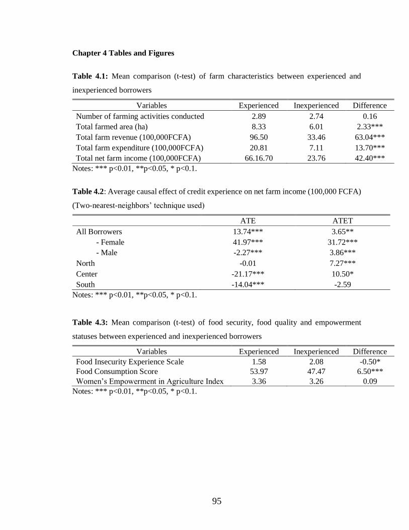
95

Chapter 4 Tables and Figures

Table 4.1: Mean comparison (t-test) of farm characteristics between experienced and

inexperienced borrowers


Number of farming activities conducted 2.89 2.74 0.16

Total farmed area (ha) 8.33 6.01 2.33***

Total farm revenue (100,000FCFA) 96.50 33.46 63.04***

Total farm expenditure (100,000FCFA) 20.81 7.11 13.70***

Total net farm income (100,000FCFA) 66.16.70 23.76 42.40***

Notes: *** p<0.01, **p<0.05, * p<0.1.

Table 4.2: Average causal effect of credit experience on net farm income (100,000 FCFA)

(Two-nearest-neighbors’ technique used)

ATE ATET

All Borrowers 13.74*** 3.65**

- Female 41.97*** 31.72***

- Male -2.27*** 3.86***

North -0.01 7.27***

Center -21.17*** 10.50*

South -14.04*** -2.59

Notes: *** p<0.01, **p<0.05, * p<0.1.

Table 4.3: Mean comparison (t-test) of food security, food quality and empowerment

statuses between experienced and inexperienced borrowers


Food Insecurity Experience Scale 1.58 2.08 -0.50*

Food Consumption Score 53.97 47.47 6.50***

Women’s Empowerment in Agriculture Index 3.36 3.26 0.09

Notes: *** p<0.01, **p<0.05, * p<0.1.

96

Table 4.4: Average causal effect of experience with farm loan on food security status (FIES

score) (Two-nearest-neighbors’ technique used)

ATE ATET

All Borrowers -0.69*** -0.24***

- Female -1.65*** -0.43***

- Male -1.04*** -1.00***

North -0.37*** -0.30***

Center -0.60*** -1.48***

South -1.28*** 1.44***

Table 4.5: Average causal effect of experience with farm loan on food quality (FCS) (Two-

nearest-neighbors’ technique used)

ATE ATET

All Borrowers 3.73*** 2.29***

- Female 10.88*** 1.32

- Male 3.99*** 3.89***

North 5.38*** 7.42***

Center 7.86*** 3.31***

South 4.80*** 2.82***

Table 4.6: Average causal effect of experience with farm loan women’s empowerment

(WEAI) (Two-nearest-neighbors’ technique used)

ATE ATET

All Borrowers 0.44*** 0.17***

North

Center

South

Given the small number of female respondent per region, there was not sufficient information to estimate

the ATE and the ATET per region.

97

Figure 4.1: Shares of loan repurposed by region (%)


matched data (Net farm income)

- ATE estimation

0

5

10

15

20

25

30

35

North Center South

Per

centa

ge

(%)

Share of loan repurposed0

.2.4

.6.8

1

Raw Matched

control treated

Pro

pensity S

core

Balance plot

Pro

pe

nsity s

co

re

02

46

0 .5 1 0 .5 1

Raw Matched

control treated

Density

Propensity Score

Balance plot

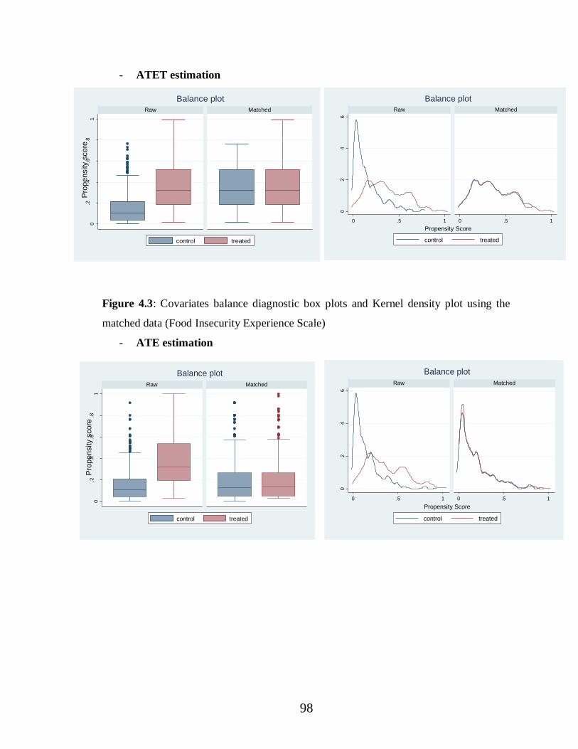
98

- ATET estimation


matched data (Food Insecurity Experience Scale)

- ATE estimation

0.2

.4.6

.81

Raw Matched

control treated

Pro

pensity S

core

Balance plot

Pro

pe

nsity s

co

re

02

46

0 .5 1 0 .5 1

Raw Matched

control treated

Density

Propensity Score

Balance plot

02

46

0 .5 1 0 .5 1

Raw Matched

control treated

Density

Propensity Score

Balance plot

0.2

.4.6

.81

Raw Matched

control treated

Pro

pensity S

core

Balance plot

Pro

pe

nsity s

co

re

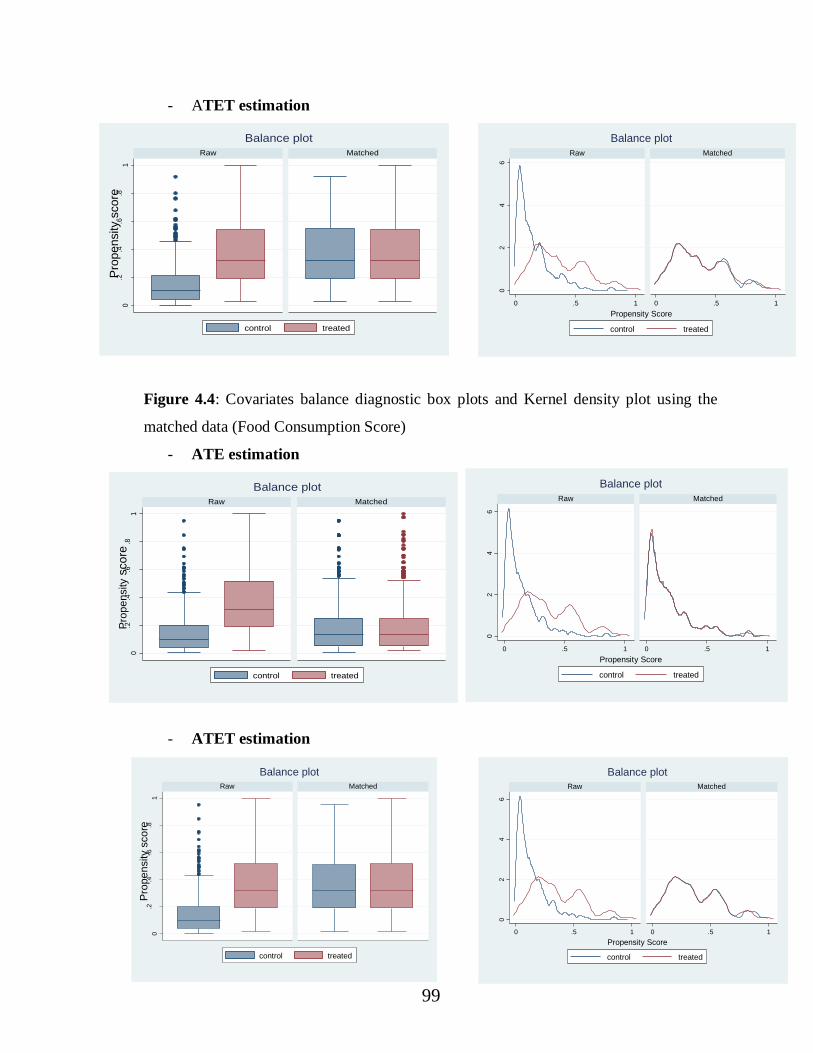
99

- ATET estimation


matched data (Food Consumption Score)

- ATE estimation

- ATET estimation

0.2

.4.6

.81

Raw Matched

control treated

Pro

pensi

ty S

core

Balance plot

Pro

pensity s

core

02

46

0 .5 1 0 .5 1

Raw Matched

control treated

Density

Propensity Score

Balance plot0

.2.4

.6.8

1

Raw Matched

control treated

Pro

pensi

ty S

core

Balance plot

Pro

pe

nsity s

core

02

46

0 .5 1 0 .5 1

Raw Matched

control treated

Density

Propensity Score

Balance plot

0.2

.4.6

.81

Raw Matched

control treated

Pro

pensity S

core

Balance plot

Pro

pe

nsity s

co

re

02

46

0 .5 1 0 .5 1

Raw Matched

control treated

Density

Propensity Score

Balance plot

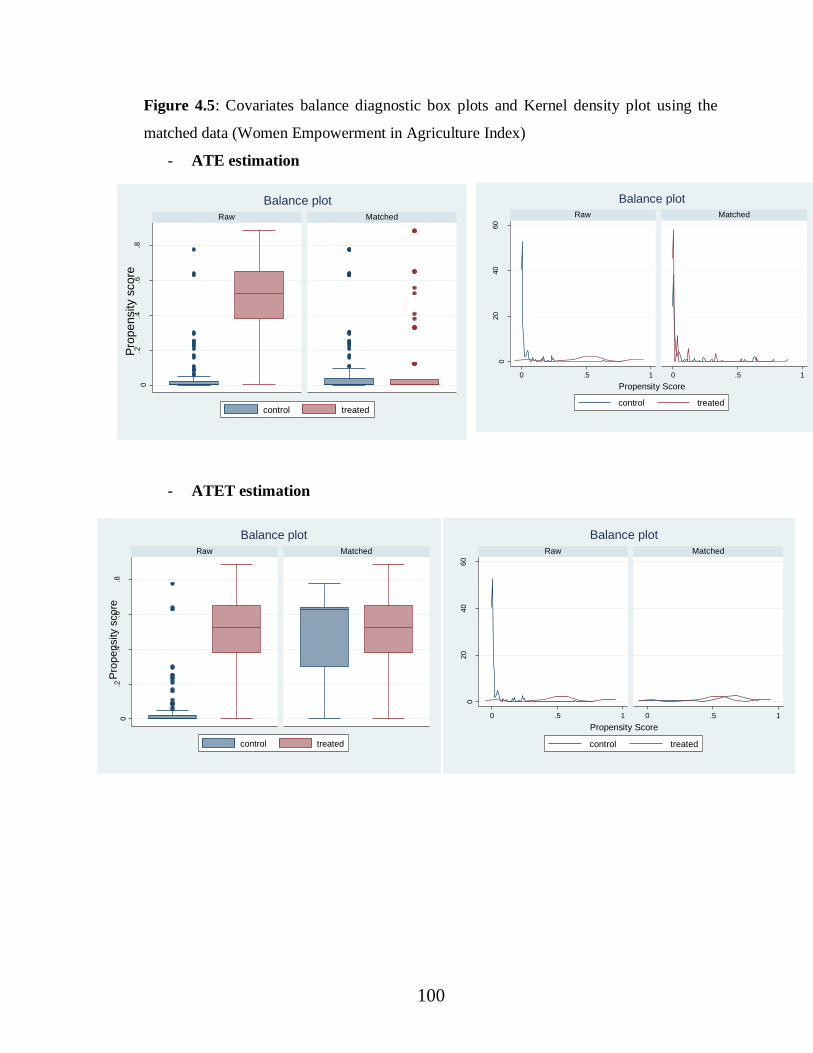
100


matched data (Women Empowerment in Agriculture Index)

- ATE estimation

- ATET estimation

0.2

.4.6

.8

Raw Matched

control treated

Pro

pensity S

core

Balance plot

Pro

pensity s

core

020

40

60

0 .5 1 0 .5 1

Raw Matched

control treated

Density

Propensity Score

Balance plot

0.2

.4.6

.8

Raw Matched

control treated

Pro

pensity S

core

Balance plot

Pro

pe

nsity s

co

re

020

40

60

0 .5 1 0 .5 1

Raw Matched

control treated

Density

Propensity Score

Balance plot

101

Figure 4.6: Overlap check for matching – Net farm income

Figure 4.7: Overlap check for matching – FIES score

102

Figure 4.8: Overlap check for matching – FCS score

Figure 4.9: Overlap check for matching – WEAI

103

General conclusion and discussion

In development economics, a basic hypothesis is that more capital inputs are

needed, not only at the aggregate level but also at the individual producer level to improve

the agricultural sector (Colyer and Jimenez, 1971). Microfinance, and more specifically,

microcredit programs, have been supported as sustainable interventions with the potential

to alleviate poverty (Pankhurst and Johnston, 1999). However, the allocation of investment

funds to farmers, especially those located in rural areas, is quite challenging. For capital to

be effectively used by farmers, it is essential to invest in human capital and correct

deficiencies in farmers’ capability (Colyer and Jimenez, 1971). In developed countries such

as the United-States of America, supervised credit programs had proven to help battle

chronical poverty in rural areas (Roberts, 2013). FECECAM the largest microlender in

Benin has been providing loans to farmers and non-farmers since 1977. Over time, the

lender has improved and adjusted its loan programs’ implementation. The Federal German

Ministry of Economic Cooperation and Development (BMZ), through the German

Financial Cooperation (KfW), has refinanced FECECAM in its effort to supporting rural

credit in general and agricultural credit in particular and is interested in furthering their

support to the lender. Though before, the KfW wants to examine the merit of supporting

the provision of loans to the rural world. The goal of this study commissioned and funded

by the KfW is to evaluate the impact of agricultural loans on the livelihoods of recipients.

Impact evaluation in the case of microcredit programs is often challenging due to

two levels of selection: self-selection into a microfinance program by the borrowers, and

the screening process of the microfinance institution. To address these biases, this study

employs the so-called pipeline design, which is typically used in a cross-sectional setting

in the absence of fully randomized experiments. This approach is justified by the fact that

both its control and treatment groups consist of individuals who have chosen to participate

in the microfinance program, addressing these two major sources of selection bias. Giving

the relatively long period studied, the analysis has been innovative in defining the loan

treatment along with creating reliable treatment groups. The loan treatment considered is

the experience with loans which includes program entry timing, loan take-up frequency

and the average amount of loan obtained over the 2012-2017’s period. To create reliable

comparable groups, the study employs a cluster analysis technique.

104

To assess the impact of FECECAM loans on clients’ livelihoods, multiple variables

and indicators are analyzed. The dissertation starts by providing a descriptive analysis of

the impact of farm loans on farmer’s labor use. The impact of loan is often discussed at the

recipient level but the second chapter of the dissertation looks beyond. It examines the role

of agricultural loans in farmers’ labor input choice. The effect of farm credit on

employment is of great importance, not only for the farmers themselves but also at the

macroeconomic level. The results of the chapter show that impact of agricultural loans on

labor is quite mixed. It suggests that past loans, clearly have residual effects on both hired

and family labor use. However, loans specifically obtained for farm machinery

significantly reduce expenditure on hired labor but more family labor is employed using

machine loans while other loan categories reduced the use of family labor. Results from

the chapter also bring up the question of the growing scarcity of labor force in rural areas,

which is due to multiple reasons including rural flight but positive ones such as increased

children schooling. Taking into account regional heterogeneities in the analysis of the

chapter offers interesting perspectives. In areas where labor is more expensive, and farm

areas are larger (North), farmers invest more in agricultural machines or technologies and

employ more family labor. In areas with affordable and better labor availability, farmers

increase their expenditure on hired labor. Certainly, loan availability made it possible for

recipients to invest in technologies and agricultural machines to avoid exhausting manual

work.

The third chapter of the dissertation evaluates the impact of agricultural loans on

the whole-farm efficiency of borrowers. Beyond the monetary benefit of loans, this chapter

examines the potential human capacity building and the knowledge gaining aspect of

extended exposure to loan programs such as FECECAM’s. Because rural finance programs

are subsidized using limited taxpayer money, it is necessary to evaluate how they affect

the marginal productivity of recipients. Results from chapter 3 indicate that lack of funds

is not the most critical problem faced by most farmers in developing countries such as

Benin. Adams and von Pischke (1991) reached the same conclusion. Even though sampled

farmers have had a relatively long period of access to credit and loan take-up, they still

display low levels of profit efficiency–the ability to produce the highest possible output at

the lowest cost. Land tenure, lack of extension services, low yields, modern inputs

105

availability and costs, output prices, risk, and weather turn out to be more critical factors

limiting farmers’ productivity and development. The third chapter also shows that the

monitoring, the technical assistance, and the training that accompany FECECAM’s loan

program may be instrumental, perhaps the key to the results. In most branches, the lender

offers tailored technical support to its clients, depending on their activities, once they are

approved for a loan. Female lending groups receive special attention and assistance from

the cooperative. FECECAM also offers specific and targeted loans and deploys a rigorous

monitoring mechanism to ensure that loans are correctly being utilized. To guarantee a high

repayment rate (93.87% as of December 2017), the cooperative uses innovative approaches

and regularly organizes recovery missions to collect outstanding loans. Though all this

contributes to the “success” of the loan program, it is costly to the loan provider, raising

the issues of providing affordable financial services to the poor and running a financially

sustainable loan program. Mobile financial services could be a solution to cost reduction

for a microlender such as FECECAM.

Finally, in the fourth chapter, long-term direct benefits of loan use are analyzed.

The chapter estimated the average causal effect of FECECAM loans on its clients’ well-

being measured by net farm income, food insecurity experience scale, food consumption

scores, and women’s empowerment in agriculture index. These are commonly studied

outcome variables when it comes to credit impact assessment. Here they are argued to

pertain to longer-term effects of agricultural loans. The positive impact of loan experience

found in the case of all studied indicators is interesting. FECECAM’s loan implementation

and monitoring practices play undoubtedly a key role here. When agricultural loans are

obtained and properly used for a purpose that was initially evaluated and planned, there are

higher chances that these loans would deliver expected results such as improving income,

which may allow to improve food security or food quality status and help gain some

autonomy. The chapter provides a simple yet valuable lesson for future impact credit

evaluation studies: the context of the loan program as well as the evaluation indicators are

essential. Not detecting an effect on a specific variable does not necessarily means the

unworthiness of microcredit in battling poverty in developing countries.

Overall, FECECAM loan program can use some improvements. The MFI could

better target rural female and their activities. The study shows that studied female

106

borrowers tend to move away from crop production towards value-adding activities

(processing and trade) as their income improves. FECECAM could also improve its level

of support to farmers by providing or facilitating their access to more technical assistance.

More, the use of mobile technologies could help the cooperative reduce the cost of

operation in some cases.

107

References

Adams, D. W., & von Pischke, J. D. (1991). Microenterprise Credit Programs: Déjà Vu,

22.

Adechoubou, M. A. (1996). Les banquiers ambulants au Bénin. Revue Tiers Monde,

37(145), 59–66. https://doi.org/10.3406/tiers.1996.5028

Aigner, D., Lovell, C. A. K., & Schmidt, P. (1977). Formulation and estimation of

stochastic frontier production function models. Journal of Econometrics, 6(1), 21–

37. https://doi.org/10.1016/0304-4076(77)90052-5

Ali, F., Parikh, A., & Shah, M. (1994). Measurement of profit efficiency using behavioural

and stochastic frontier approaches. Applied Economics, 26(2), 181–188.

https://doi.org/10.1080/00036849400000074

Ali, Mubarak, & Byerlee, D. (1991). Economic efficiency of small farmers in a changing

world: A survey of recent evidence. Journal of International Development, 3(1), 1–

27. https://doi.org/10.1002/jid.4010030102

Ali, Mubarik, & Flinn, J. C. (1989). Profit Efficiency among Basmati Rice Producers in

Pakistan Punjab. American Journal of Agricultural Economics, 71(2), 303–310.

https://doi.org/10.2307/1241587

Amouzou, K. (2008). Analyse de l’efficacité sociale des IMF au Bénin. Université

d’Abomey-Calavi - Ecole Nationale d’Economie Appliquée et de Management

(ENEAM), Benin.

Angelucci, M., Karlan, D., & Zinman, J. (2015). Microcredit Impacts: Evidence from a

Randomized Microcredit Program Placement Experiment by Compartamos Banco.

American Economic Journal: Applied Economics, 7(1), 151–182.

https://doi.org/10.1257/app.20130537

Armendáriz de Aghion, B., & Morduch, J. (2000). Microfinance beyond group lending.

Economics of Transition, 8(2), 401–420.

Armendáriz de Aghion, B., & Morduch, J. (2005). The Economics of Microfinance.

Cambridge, Massachusetts: The MIT Press.

Balsvik, R. (1995). Production decisions in nonpooling households (Memorandum from

Department of Economics No. No 7). Norway: University of Oslo.

Banerjee, A., Duflo, E., Glennerster, R., & Kinnan, C. (2014). The miracle of

microfinance? Evidence from a randomized evaluation (NBER Working Paper No.

18950) (pp. 1–53). USA: National Bureau of Economic Research.

Batra, V. (2010). Impact of microfinance on rural women: A case study of Haryana (Thesis

submitted for the degree of Doctor of Philosophy). Maharshi Dayanand University,

India. Retrieved from

http://shodhganga.inflibnet.ac.in:8080/jspui/handle/10603/113571

Battese, G. E., & Coelli, T. J. (1995). A model for technical inefficiency effects in a

stochastic frontier production function for panel data. Empirical Economics, 20(2),

325–332. https://doi.org/10.1007/BF01205442

108

Battese, G. E., & Corra, G. S. (1977). Estimation of a Production Frontier Model: With

Application to the Pastoral Zone of Eastern Australia. Australian Journal of

Agricultural Economics, 21(3), 169–179. https://doi.org/10.1111/j.1467-

8489.1977.tb00204.x

Becker, G. S. (1965). A Theory of the Allocation of Time. The Economic Journal, 75(299),

493–517. https://doi.org/10.2307/2228949

Benin Data Portal. (2016). Principaux Indicateurs RGPH 2013 - Benin. Retrieved

September 12, 2018, from http://benin.opendataforafrica.org//ohikebf/principaux-

indicateurs-rgph-2013-benin?region=1000020-atacora&indicateur=1001240-

taille-moyenne-des-m%C3%A9nages

Besley, T., & Coate, S. (1995). Group lending, repayment incentives and social collateral.

Journal of Development Economics, 46, 1–18.

Binswanger, H. P., & McIntire, J. (1987). Behavioral and Material Determinants of

Production Relations in Land-abundant Tropical Agriculture. Economic

Development & Cultural Change, 36(1), 73.

Binswanger-Mkhize, H. P., & Savastano, S. (2017). Agricultural intensification: The status

in six African countries. Food Policy, 67, 26–40.

https://doi.org/10.1016/j.foodpol.2016.09.021

Blume, J., & Breyer, J. (2011). Microfinance and Child Labour. Geneva: International

Labour Office, Employment Sector, Social Finance Programme. Retrieved from

https://pdfs.semanticscholar.org/1ef1/2330bb3f3ab91d502dcda130eb27aa472f2a.

pdf

Boserup, E. (1965). The Conditions of Agricultural Growth: The Economics of Agrarian

Change Under Population Pressure (2003 Reprint, Vol. 4). London: Psychology

Press.

Brake, J. R. (1974). A Perspective on Federal Involvement in Agricultural Credit Programs.

South Dakota Law Review, 19, 567.

Bravo-Ureta, B. E., & Pinheiro, A. E. (1993). Efficiency Analysis Of Developing Country

Agriculture: A Review Of The Frontier Function Literature. Agricultural and

Resource Economics Review, 22(1), 88–101.

Bravo-Ureta, B. E., & Rieger, L. (1991). Dairy Farm Efficiency Measurement Using

Stochastic Frontiers and Neoclassical Duality. American Journal of Agricultural

Economics, 73(2), 421–428. https://doi.org/10.2307/1242726

Brosnan, J. (2016, February 4). Partnerships for Progress: Benin Could Benefit from

Financial Sector Coordination [Text]. Retrieved July 24, 2017, from

http://finclusionlab.org/blog/partnerships-progress-benin-could-benefit-financial-

sector-coordination

Bylander, M. (2015). Credit as Coping: Rethinking Microcredit in the Cambodian Context.

Oxford Development Studies, 43(4), 533–553.

http://dx.doi.org/10.1080/13600818.2015.1064880

109

Cai, H., Chen, Y., Fang, H., & Zhou, L.-A. (2015). The Effect of Microinsurance on

Economic Activities: Evidence from a Randomized Field Experiment. The Review

of Economics and Statistics, 97(2), 287–300.

https://doi.org/10.1162/REST_a_00476

Charnes, A., Cooper, W. W., & Rhodes, E. (1978). Measuring the efficiency of decision

making units. European Journal of Operational Research, 2(6), 429–444.

https://doi.org/10.1016/0377-2217(78)90138-8

Christiaensen, L., Demery, L., & Kuhl, J. (2011). The (evolving) role of agriculture in

poverty reduction—An empirical perspective. Journal of Development Economics,

96(2), 239–254. https://doi.org/10.1016/j.jdeveco.2010.10.006

Coelli, T. J. (1995). Recent Developments in Frontier Modelling and Efficiency

Measurement. Australian Journal of Agricultural Economics, 39(3), 219–245.

https://doi.org/10.1111/j.1467-8489.1995.tb00552.x

Coleman, B. E. (1999). The impact of group lending in Northeast Thailand. Journal of

Development Economics, 60(1), 105–141. https://doi.org/10.1016/S0304-

3878(99)00038-3

Coleman, B. E. (2006). Microfinance in Northeast Thailand: Who benefits and how much?

World Development, 34(9), 1612–1638.

https://doi.org/10.1016/j.worlddev.2006.01.006

Colyer, D., & Jimenez, G. (1971). Supervised Credit as a Tool in Agricultural

Development. American Journal of Agricultural Economics, 53(4), 639–642.

https://doi.org/10.2307/1237828

Copestake, J., Bhalotra, S., & Johnson, S. (2001). Assessing the impact of microcredit: A

Zambian case study. Journal of Development Studies, 37(4), 81–100.

https://doi.org/10.1080/00220380412331322051

Crépon, B., Devoto, F., Duflo, E., & Parienté, W. (2015). Estimating the Impact of

Microcredit on Those Who Take It Up: Evidence from a Randomized Experiment

in Morocco. American Economic Journal: Applied Economics, 7(1), 123–150.

https://doi.org/10.1257/app.20130535

Cui, Q., Dieterich, C., & Maino, R. (2016). Benin (IMF Country Report No. 16/7) (pp. 1–

25). Washington D.C.: International Monetary Fund.

Dethier, J.-J., & Effenberger, A. (2012). Agriculture and development: A brief review of

the literature. Economic Systems, 2(36), 175–205.

https://doi.org/10.1016/j.ecosys.2011.09.003

Duvendack, M., Palmer-Jones, R., Copestake, J. G., Hooper, L., Loke, Y., & rao, N. (2011).

What is the evidence of the impact of microfinance on the well-being of poor

people? London, UK: EPPI-Centre, Social Science Research Unit, Institute of

Education, University of London.

110

Ellrich, J., & Sarges, B. (2010). Microfinance on the Rise - A Socially Inspired Business

Model about to Emerge into an Asset Class (pp. 1–4). Arthur D. Little. Retrieved

from www.adl.com/microfinancerise

Erhardt, E. (2017). Microfinance beyond self-employment: Evidence for firms in Bulgaria.

Labour Economics, In press. Retrieved from

http://dx.doi.org/10.1016/j.labeco.2017.04.009

Fafchamps, M. (2002). Intrahousehold access to land and sources of inefficiency: theory

and concept. In A. de Janvry, G. Gordillo, J. ‐P. Platteau, & E. Sadoulet (Eds.),

Land Reform Revisited: Access to Land, Rural Poverty and Public Action. Oxford

University Press.

Fafchamps, M., & Quisumbing, A. R. (2003). Social Roles, Human Capital, and the

Intrahousehold Division of Labor: Evidence from Pakistan. Oxford Economic

Papers, 55(1), 36–80.

FAO. (2002). The role of agriculture in the development of least-developed countries and

their integration into the world economy (p. 190). Rome, Italy: Food and

Agriculture organization - Commodities and Trade division. Retrieved from

http://www.fao.org/docrep/007/Y3997E/Y3997E00.HTM

Farrell, M. J. (1957). The Measurement of Productive Efficiency. Journal of the Royal

Statistical Society. Series A (General), 120(3), 253–290.

https://doi.org/10.2307/2343100

Feder, G., Lau, L. J., Lin, J. Y., & Luo, X. (1990). The Relationship between Credit and

Productivity in Chinese Agriculture: A Microeconomic Model of Disequilibrium.

Oxford University Press on Behalf of the Agricultural & Applied Economics

Association, 72(5), 1151–1157.

Førsund, F. R., Lovell, C. A. K., & Schmidt, P. (1980). A survey of frontier production

functions and of their relationship to efficiency measurement. Journal of

Econometrics, 13(1), 5–25. https://doi.org/10.1016/0304-4076(80)90040-8

Gaile, G., & Foster, J. (1996). Review of the Methodological Approaches to the Study of

the Impact of Microenterprise Credit Programs (Working Paper) (p. 58). USAID -

Assessing the Impact of Microenterprise Services. Retrieved from

http://www.microfinancegateway.org/library/review-methodological-approaches-

study-impact-microenterprise-credit-programs

Gastellu, J.-M. (1979). Mais où sont donc ces unités économiques que nos amis cherchent

tant en Afrique ? But where are these economic units that our friends are seeking

so much in Africa? (Note AMIRA No. N° 26) (pp. 1–24). Abidjan, Côte d’Ivoire:

Office de la Recherche Scientifique et Technique Outre Mer.

Girabi, F., & Mwakaje, A. E. G. (2013). Impact of Microfinance on Smallholder farm

productivity in Tanzania : The case of Iramba District. Asian Economic and

Financial Review, 3(2), 227–242.

111

Godquin, M. (2004). Microfinance Repayment Performance in Bangladesh: How to

Improve the Allocation of Loans by MFIs. World Development, 32(11), 1909–

1926. https://doi.org/10.1016/j.worlddev.2004.05.011

Gomez, R., & Santor, E. (2003). Do Peer Group Members Outperform Individual

Borrowers?: A Test of Peer Group Lending Using Canadian Micro-credit Data.

Bank of Canada.

Grameen Foundation. (2016). Financial Services. Retrieved from

https://www.grameenfoundation.org/what-we-do/financial-services

Guttman, J. M. (2007). Repayment Performance in Microcredit Programs: Theory and

Evidence (SSRN Scholarly Paper No. ID 985890). Rochester, NY: Social Science

Research Network. Retrieved from https://papers.ssrn.com/abstract=985890

Hazarika, G., & Sarangi, S. (2008). Household Access to Microcredit and Child Work in

Rural Malawi. World Development, 36(5), 843–859.


Heckman, J. (1997). Instrumental Variables: A Study of Implicit Behavioral Assumptions

Used in Making Program Evaluations. The Journal of Human Resources, 32(3),

441–462. https://doi.org/10.2307/146178

Houngan, S. (2015). Impact des crédits octroyés par les institutions de microfinance sur le

niveau de vie des bénéficiaires : cas du Bénin (Impact of loans granted by

microfinance institutions on the living standard of beneficiaries: the case of Benin)

(Mémoire de fin de formation du Master en Economie publique et statistique

appliquée). Institut de Recherche Empirique e Economie Politique (IREEP), Benin.

Hunt, D. (1991). Farm system and household economy as frameworks for prioritising and

appraising technical research: a critical appraisal of current approaches. In M.

Haswell & D. Hunt (Eds.), Rural Households in Emerging Societies: Technology

and Change in Sub-Saharan Africa. Bloomsbury Academic.

INSAE. (2009). Enquête Modulaire Intégrée sur les Conditions de vie des Ménages

(EMICoV) Bénin 2007 - Rapport Général d’Analyse (pp. 1–290). Cotonou, Bénin:

Institut National de la Statistique et de l’Analyse Économique.

Iversen, V. (2002). Idiosyncrasies of child labour in peasant households in sub-Saharan

Africa: anthropological observations and the economics of labour obligations and

exchange. Unpublished, University of East Anglia, Norwich.

Joseph, A. (2002). La réforme du secteur financier en Afrique. OECD Publishing, 71.

http://dx.doi.org/10.1787/463385011306

Kabeer, N. (1999). Resources, Agency, Achievements: Reflections on the Measurement of

Women’s Empowerment. Development and Change, 30(3), 435–464.

https://doi.org/10.1111/1467-7660.00125

Karlan, D., Osei, R., Osei-Akoto, I., & Udry, C. (2014). Agricultural decisions after

relaxing credit and risk constraints. The Quarterly Journal of Economics, 129(2),

597–652. https://doi.org/10.1093/qje/qju002

112

Karlan, D. S. (2001). Microfinance Impact Assessments: The Perils of Using New

Members as a Control Group. Journal of Microfinance, 3(2). Retrieved from

http://scholarsarchive.byu.edu/esr/vol3/iss2/5

Karlan, D., & Tedeschi, G. A. (2010). Cross sectional impact analysis: Bias from dropouts.

Perspectives on Global Development and Technology, 9(3–4), 270 – 291.

https://doi.org/10.1163/156914910X499714

Karlan, D., & Zinman, J. (2011). Microcredit in Theory and Practice: Using Randomized

Credit Scoring for Impact Evaluation. Science, 332, 1278–1284.

https://doi.org/10.1126/science.1200138

Kodongo, O., & Kendi, L. G. (2013). Individual lending versus group lending: An

evaluation with Kenya’s microfinance data. Review of Development Finance, 3,

99–108.

Kopp, R. J., & Diewert, W. E. (1982). The decomposition of frontier cost function

deviations into measures of technical and allocative efficiency. Journal of

Econometrics, 19(2), 319–331. https://doi.org/10.1016/0304-4076(82)90008-2

Kopp, R. J., & Smith, V. K. (1980). Frontier Production Function Estimates for Steam

Electric Generation: A Comparative Analysis. Southern Economic Journal, 46(4),

1049–1059. https://doi.org/10.2307/1057240

Kumbhakar, S. C. (1996). Efficiency Measurement with Multiple Outputs and Multiple

Inputs. Journal of Productivity Analysis, 7(2/3), 225–255.

Kumbhakar, S. C., Ghosh, S., & McGuckin, J. T. (1991). A Generalized Production

Frontier Approach for Estimating Determinants of Inefficiency in U.S. Dairy

Farms. Journal of Business & Economic Statistics, 9(3), 279–286.

https://doi.org/10.1080/07350015.1991.10509853

Lamarche, H. (1991). L’Agriculture familiale: Une réalité polymorphe (Vol. 1).

L’Harmattan.

Lélart, M. (2007). Les mutations dans la microfinance - L’expérience du Bénin (Document

de Recherche No. N° 2007-15) (p. 24). Orléans, France: Laboratoire d’Economie

d’Orléans.

MAEP. (2011). Plan Stratégique de Relance du Secteur Agricole (PSRSA) (p. 112 p).

Cotonou, Bénin: Ministère de l’Agriculture, de l’Elevage et de la Pêche (MAEP).

MAEP. (2017). Plan Stratégique de Dévelopment du Secteur Agricole (PSDSA) et Plan

National d’Investissements Agricoles et de Sécurité Alimentaire et Nutritionnelle

(PNIASAN) 2017 - 2021. Retrieved July 7, 2018, from

http://agriculture.gouv.bj/spip.php?article332

Makles, A. (2012). Stata tip 110: How to get the optimal k-means cluster solution. The

Stata Journal, 12(2), 347–351.

Maldonado, J. H., & González-Vega, C. (2008). Impact of Microfinance on Schooling:

Evidence from Poor Rural Households in Bolivia. World Development, 36(11),

2440–2455. https://doi.org/10.1016/j.worlddev.2008.04.004

113

Marr, A. (2012). Effectiveness of Rural Microfinance: What We Know and What We Need

to Know. Journal of Agrarian Change, 12(4), 555–563.

Mazumder, M. S. U., & Lu, W. (2015). What Impact Does Microfinance Have on Rural

Livelihood? A Comparison of Governmental and Non-Governmental Microfinance

Programs in Bangladesh. World Development, 68, 336–354.


MEF. (2016). Ministère de l’Économie et des Finances : Microfinance. Retrieved June 16,

2017, from http://www.finances.bj/thematiques/economie/microfinance/

MEF. (2017). Ministère de l’Économie et des Finances : Microfinance. Retrieved January

25, 2018, from

http://www.finances.bj/fr/thematiques/economie/microfinance/?tx_wdbiblio_pi1

%5Bcategory%5D=7&tx_wdbiblio_pi1%5Bmode%5D=1&tx_wdbiblio_pi1%5B

pointer%5D=7&cHash=48eef7a804dd72a959217177508ed382

Mendola, M. (2007). Farm Household Production Theories: A Review of “Institutional”

and “Behavioral” Responses. Asian Development Review, 24(1), 49–68.

Mohsin, A. Q., Ahmad, S., & Anwar, A. (2011). Impact of Supervised Agricultural Credit

on Farm Income in the Barani Areas of Punjab. Pakistan Journal of Social Sciences,

31(02), 241–250.

MSC. (2012). State of the Microcredit Summit Campaign Report 2012 (No. ISBN 978-0-

9763704-7-5) (pp. 1–74). Washington D.C., USA: Microcredit Summit Campaign.

Muller, B., Sall, M., Leblois, A., Balde, A., Fall, M., Kouakou, P., & Affholder, F. (2013).

L’assurance agricole indicielle en afrique de l’ouest : principes, premières

réalisations et perspectives. Agronomie Africaine, Numéro spécial(6), 95–111.

Odell, K. (2015). Measuring the impact of microfinance: Looking to the future (Paper No.

No3) (p. 60). Grameen Foundation.

Otero, M. (1999). Bringing Development Back into Microfinance. Journal of

Microfinance, 1(1), 1–12.

Owitti, O. L. (2015). Gender Differences and Relations in Rural Household Livelihoods of

Gog District, Anywaa Zone, Gambella Region, South Western Ethiopia.

International Journal of Gender and Women’s Studies, 3(1), 51–79.

https://doi.org/10.15640/ijgws.v3n1p7

Pankhurst, H., & Johnston, D. (1999). Diversity in Practice: An international NGO’s

experience of micro-finance. In S. Jones & N. Nelson (Eds.), Urban Poverty in

Africa: From Understanding to Alleviation (pp. 91–101). Intermediate Technology.

Pitcher, M. A. (1996). Conflict and Cooperation: Gendered Roles and Responsibilities

within Cotton Households in Northern Mozambique. African Studies Review,

39(3), 81–112. https://doi.org/10.2307/524944

Pitt, M. M., & Khandker, S. R. (1998). The Impact of Group-Based Credit Programs on

Poor Households in Bangladesh: Does the Gender of Participants Matter? Journal

of Political Economy, 106(5), 958–996.

114

PLURIEX. (2011). Mission D’évaluation Globale Du Programme De Micro-Crédit Aux

Plus Pauvres (PMCPP) - Rapport final (Rapport de consultation) (pp. 1–88).

Benin: Fonds National de la Microfinance - FNM.

PNUD-Bénin. (2007). Diagnostic Approfondi Du Secteur De La Microfinance Au Bénin

(Rapport d’étude) (pp. 1–66). Benin: Programme des Nations Unies pour le

Développement (PNUD).

Rajbanshi, R., Huang, M., & Wydick, B. (2015). Measuring Microfinance: Assessing the

Conflict between Practitioners and Researchers with Evidence from Nepal. World

Development, 68, 30–47.

Roberts, C. K. (2013). Client Failures and Supervised Credit in the Farm Security

Administration. Agricultural History, 87(3), 368–390.

https://doi.org/10.3098/ah.2013.87.3.368

Roodman, D., & Morduch, J. (2014). The Impact of Microcredit on the Poor in Bangladesh:

Revisiting the Evidence. The Journal of Development Studies, 50(4), 583–60.

https://doi.org/10.1080/00220388.2013.858122

Rosenbaum, P. R., & Rubin, D. B. (1983). The central role of the propensity score in

observational studies for causal effects. Biometrika, 70(1), 41–55.

Ruthenberg, H. (1971). Farming systems in the tropics. Oxford: Clarendon Press.

Sasse, A. (2016, May 17). Benin cotton sector wary as government hands back control.

Reuters. Retrieved from https://af.reuters.com/article/topNews/idAFKCN0Y81Y4

Schmidt, P. (1985). Frontier production functions. Econometric Reviews, 4(2), 289–328.

https://doi.org/10.1080/07474938608800089

Shankar, S. (2007). Transaction costs in group microcredit in India. Management Decision,

45(8), 1331–1342. https://doi.org/10.1108/00251740710819069

Sow, F. D. (2010). Intrahousehold Resource Allocation and Well-being: The Case of Rural

Households in Senegal. Wageningen Academic Publishers.

Stiglitz, J. E. (1990). Peer Monitoring and Credit Markets. The World Bank Economic

Review, 4(3), 351–366.

Taylor, E. J., & Adelman, I. (2003). Agricultural Household Models: Genesis, Evolution,

and Extensions. Review of Economics of the Household, 1(1), 33–58.

The World Bank. (2016, September). Benin Overview. Retrieved March 22, 2017, from

https://www.worldbank.org/en/country/benin/overview

The World Bank. (2018, April). The World Bank in Benin - Overview [Text/HTML].

Retrieved November 15, 2018, from

http://www.worldbank.org/en/country/benin/overview

Thomas, D. (1990). Intra-Household Resource Allocation: An Inferential Approach. The

Journal of Human Resources, 25(4), 635–664. https://doi.org/10.2307/145670

UN-DESA. (2010). Population Facts (No. 2010/5) (pp. 1–4). United Nations Department

of Economic and Social Affairs - Population Division. Retrieved from

115

http://www.un.org/en/development/desa/population/publications/pdf/popfacts/pop

facts_2010-5.pdf

UNESCO. (2016, November 27). Benin - Participation in Education. Retrieved February

21, 2019, from http://uis.unesco.org/en/country/bj

Village Invest. (2016). What is microfinance? Retrieved March 2, 2018, from

https://www.villageinvest.com/about/village-invest-difference/what-microfinance

Wang, J., Cramer, G. L., & Wailes, E. J. (1996). Production efficiency of Chinese

agriculture: evidence from rural household survey data. Agricultural Economics,

15(1), 17–28. https://doi.org/10.1016/S0169-5150(96)01192-9

Yotopoulos, P. A., & Lau, L. J. (1979). Resource Use in Agriculture: Applications of the

Profit Function to Selected Countries. Food Research Institute Studies, 17(01), 1–

132.

116

VITA

NICAISE SHEILA MAHUTIN SAGBO

Born in Cotonou, Benin

EDUCATION

Ph.D. Agricultural Economics University of Kentucky, Expected May 2019

Dissertation: “Effects of Agricultural Loans in Developing

Countries – Benin case study.”

Committee: Dr. Yoko Kusunose (Co-Director), Dr. Leigh

Maynard (Co-Director), Dr. David Freshwater, Dr.

Steven Buck, Dr. J.S. Butler, and Dr. James Fackler

December 2014: M.Sc. Agricultural Economics, University of

Kentucky

February 2011: M.Sc. Development Economics, Université

d’Abomey-Calavi, Benin

November 2009: B.Sc. Agricultural Science, Université d’Abomey-

Calavi, Benin

PROFESSIONAL EXPERIENCE

December 2018 – February 2019: Consultant, World Coffee Research, USA

August 2014 – December 2018: Research Assistant, Department of Agricultural

Economics, University of Kentucky

July 2017 – February 2018: Junior Research Analyst, Impact of Agricultural

Credit in Benin, German Development Institute

(DIE) & LADYD-University of Abomey Calavi,

Benin

July 2015 – July 2017: Research Specialist, Policy Analysis Matrix Project,

USDA & University of Kentucky, USA & Haiti

117

September – December 2013: Research Assistant, Community Supported

Agriculture Project, University of Kentucky, USA

June - August 2013: Intern, Kentucky Farm Business Management

Program (KFBM), USA

September 2011 – June 2012: Coordinator’s Assistant, Netherlands Development

Organization (SNV), Benin

July – December 2011: Research Assistant, Joint Learning About Innovation

Systems in African Agriculture Program, Benin

March – July 2011: Assistant Coordinator, Millet and Sorghum Project,

Benin

January 2009 – January 2010: Research Assistant, Benin Environment and

Economic & Social Development Center-

CEBEDES

July - October 2008: Intern, Benin Center for Environment and Economic

and Social Development – CEBEDES

June - October 2007: Intern, National Agricultural Research Institute

(INRAB), Benin

FELLOWSHIPS AND AWARDS

2017: Research grant, German Development Institute (DIE)

2014-2018: Graduate Research Assistantship, University of

Kentucky

2013: Student Sustainability Council Grant, University of

Kentucky Student Sustainability Council

2012-2014: Fulbright Scholars Program, US Department of State

2006 - 2011: Benin Government College Scholarship Program

118

CONFERENCE AND WORKING PAPERS

2018: Sagbo S., Floquet A., Bruentrup M. (2018). Impacts du crédit Agricole de la

Faîtière des Caisses d’Epargne et de Crédit Agricole Mutuel du Bénin

(FECECAM-BENIN). Cotonou (Bénin), Working paper

2016: “Does certification to private food standards improve market access? Evidence

from EU and US import refusals” Working paper.

2015: “The impact of improved clean cookstoves on households in Southern Haiti.”

Presented at the Southern Agricultural Economics Association Conference.

Atlanta, Georgia

2014: “Economic analysis and Willingness to pay for alternative charcoal and clean

cookstoves in Haiti.” Master Thesis

2013: “Factors contributing to farm management returns in Kentucky.” Presented at

the Southern Agricultural Economics Association Conference. Dallas, Texas

2012: “Inventaire des Entreprises Agricoles et Agro-business du Bénin” (Study on

agricultural businesses and agro-businesses in Benin). Technical Report.

Netherlands Development Organization

2011: “Systèmes agro-pastoraux et chaînes de valeurs ajoutées du fromage peuhl dans

les départements de l’Atacora et de la Donga au Nord Bénin” (Agro-pastoral

Systems and Fulbe Cheese Value Chains Analysis in Atacora and Donga

Departments in Northern Benin). Master Thesis

EFFECTS OF AGRICULTURAL LOANS IN DEVELOPING …

Documents

Transcript of EFFECTS OF AGRICULTURAL LOANS IN DEVELOPING …