Effective Variation Management for Pseudo Periodical Streams

Lv-an Tang1, Bin Cui2, Hongyan Li1*, 1State Key Laboratory on Machine Perception

Department of Intelligent Science School of EECS, Peking University

{Tangla,lihy,miaogs,zhouxb}@cis.pku.edu.cn

Gaoshan Miao1, Dongqing Yang2, Xinbiao Zhou1

2Department of Computer Science and Technology School of EECS, Peking University

{bin.cui, dqyang}@pku.edu.cn

ABSTRACT Many database applications require the analysis and processing of data streams. In such systems, huge amounts of data arrive rapidly and their values change over time. The variations on streams typically imply some fundamental changes of the underlying objects and possess significant domain meanings. In some data streams, successive events seem to recur in a certain time interval, but the data indeed evolves with tiny differences as time elapses. This feature is called pseudo periodicity, which poses a non-trivial challenge to variation management in data streams. This paper presents our research effort in online variation management over such streams, and the idea can be applied to the problem domain of medical applications, such as patient vital signal monitoring. We propose a new method named Pattern Growth Graph (PGG) to detect and manage variations over pseudo periodical streams. PGG adopts the wave-pattern to capture the major information of data evolution and represent them compactly. With the help of wave-pattern matching algorithm, PGG detects the stream variations in a single pass over the stream data. PGG only stores the different segments of the pattern for incoming stream, and hence it can substantially compress the data without losing important information. The statistical information of PGG helps to distinguish meaningful data changes from noise and to reconstruct the stream with acceptable accuracy. Extensive experiments on real datasets containing millions of data items demonstrate the feasibility and effectiveness of the proposed scheme.

Categories and Subject Descriptors: H.2.8 [Database Management]: Database Applications - Data Mining General Terms: Algorithms. Keywords: Date stream, variation management, pattern growth, pseudo periodicity.

1. INTRODUCTION Data stream processing techniques are widely applied in many domains such as stock market analysis, road traffic control, weather forecasting and medical information management. In the data stream model, rapidly arriving data items must be processed online, and the stream shows trends of variation as time elapses. These variations often imply fundamental changes about the underlying

objects and possess high domain significance. Most existing stream processing methods focus on traditional SQL queries, which cannot be employed for detecting variations or finding patterns. Moreover, time series mining algorithms are also not adequate for managing variations over data stream, either consuming too much time or requiring complete training sets.

Online variation management is an important task in data stream mining, and has attracted increasing attention recently [1-4]. However, few results have been achieved due to three major technical challenges [5].

Complexity of Value Type: Most stream mining tasks are based on discrete and enumerative values or time series data with equidistant intervals, while many meaningful variations are on consecutive data streams with variable sampling frequencies;

Non-Availability Training Sets or Models: Normally, the novelty detection in time series database is based on several training sets or predefined models. However, it is hard to get such aids over data streams because the models also evolve with time. Instead, the system is usually required to generate such models by itself;

High Requirements for Variation Management: The users would not be satisfied with only being told “when and how the variation occurs?”, they also want to know “why the data turns to change in this way?”. Therefore the data stream management system must report both event time and variation history to the users.

Some variations over streams have abnormal values, which can be easily handled by outlier detection techniques [6, 7, 29]. However, typical stream variations involve gradual evolutions rather than burst changes. The data seems to repeat in a certain period, whereas tiny difference exists between pair of consecutive periods, either the key value or the time interval. This kind of stream is called pseudo periodical stream, which is very common in medical applications, such as patient vital signal monitoring. In this paper, we will only focus on the bio-medical signals, including Electrocardiograph (ECG), respiration, and so on. Although the solution is customized for medical data stream, our approach can be applied to other application domains with periodical streams, where periodicity is also common, such as economic time series, temperature with seasonal changes, and earthquake waves [31]. Here, we use an example of medical signal to illustrate the characteristic of such data stream.

Example 1: Figure 1 records the data evolution over a respiration stream. The respiratory data seems to repeat every 3.2 seconds. At the beginning, the data in time A and B are almost the same,

* Corresponding author.

Permission to make digital or hard copies of all or part of this work for personal or classroom use is granted without fee provided that copies are not made or distributed for profit or commercial advantage and that copies bear this notice and the full citation on the first page. To copy otherwise, or republish, to post on servers or to redistribute to lists, requires prior specific permission and/or a fee. SIGMOD’07, June 12–14, 2007, Beijing, China. Copyright 2007 ACM 978-1-59593-686-8/07/0006...$5.00.

257

including two inspiration sections and one expiration section. After 20 minutes, the expiration data in time C transforms to two sections. In time D (after 3 hours) and E (after 5 hours), the inspiration data merges into one section, while the expiration data evolves into three sections. The variations reflect the evolution of the patient’s illness during the five hours.

Figure 1. Pseudo Periodicity of the Respiration Stream

It is a non-trivial challenge to the data stream systems to detect and analyze this kind of variations with marginal space cost and in near real time, because the variations are not only on the values but also on the inner structure given a certain period. They can only be detected by comparing the data of two periods over a longer duration, which brings about two main problems. First, it is hard to capture the periodical data with fixed size windows or buffers, because the length of the period also evolves. Second, comparing two periods with different data sizes and time lengths is even more difficult. In many applications, these variations are monitored manually, which is costly and error-prone [19]. Therefore, it is useful and necessary to develop algorithms and tools for detecting, recording and understanding such variations over pseudo periodical data streams.

In this paper, we propose a novel approach -- Pattern Growth Graph (PGG) to manage the variations over long pseudo periodical data streams. In stream processing, variations are detected by comparing old data with an incoming stream using sequence matching. To efficiently represent the stream, we split the infinite stream into segments, and adopt wave-pattern to capture the major information of data evolution. The wave-pattern adopts line sections to approximate the data using Sliding Window And Bottom-up algorithm [34]. Additionally, an efficient wave-pattern matching algorithm is proposed to compute the difference between two stream segments. Using the wave-pattern, we can detect the stream variation in a single pass over the data, and maintain the variation history using PGG. PGG organizes the patterns with bi-directional linked lists, and only stores the different pattern parts for incoming stream if the stream pattern is different from the known Patterns in PGG. Therefore, it can compress the data substantially without losing important information. Additionally, the statistical information of PGG helps the system to distinguish meaningful data changes from noise and to reconstruct the stream with acceptable accuracy. Our contributions can be summarized as follows:

We propose to use the valley points to split a pseudo periodical stream into segments which can be represented by wave-pattern efficiently. A new pattern matching algorithm is proposed to detect variations in streams.

We introduce a novel structure PGG to record the wave patterns of the stream incrementally and maintain their evolving history with marginal space overhead.

We conduct extensive experiments to prove the effectiveness of PGG using real datasets containing millions of data items. PGG yields higher precision on variation detection with fewer false alarms than existing techniques. Most encouragingly, the proposed PGG technique has been implemented as the core module in a J2EE based data stream management system. The system is now used in a major hospital’s Intense Care Unit (ICU), monitoring over twenty patients a day.

The rest of the paper is organized as follows: Section 2 briefly discusses related work; Section 3 describes concepts and algorithms for detecting variations and recording their history in PGG; Section 4 discusses some applications of PGG; Section 5 reports the experimental results; finally we summarize the paper in Section 6.

2. RELATED WORK The research on data streams has received much attention in recent years, and most of the work can be loosely classified in two categories [8].

Data Stream Management Systems (DSMS): A large number of projects have been carried out to implement DSMS, including STREAM [9], Aurora [10], TelegraphCQ [11], Cougar [12], and so on. Although they have been applied in different domains, the goals are in common that they mainly focus on completing predefined queries over rapid streams in near real-time. Given that premise, a series of query technologies, such as scheduling, summary, load shedding, synopsis maintenance [13-16] are employed. However, as pointed out in reference [8], the emphasis of the techniques in this category is to support only traditional SQL queries. None of them tried to find the data patterns, or to monitor the variations.

To the best of our knowledge, there is no DSMS applied in domains of pseudo periodical streams, such as the domains of medicine, seismology, and so on. For instance, a typical case of such streams is the medical signals generated from the Intensive Care Unit (ICU) of hospitals. But the common systems in ICU, such as HP CareVue [17] and VA quantitative sentinel system [18], all use databases to store bio-medical signals. Due to storage limitation, they can only sample the data with a rather long interval. None of them can analyze the stream data or detect variations. The tasks of variation management are completed manually by nurses [19].

Online Data Mining Another category of the work is data mining on the stream, including clustering, classification, regression and frequent pattern mining.[1-4]

Variation management is an important part of online data mining. It has been variously referred to as the detection of “unusual subsequence” [6], “surprising pattern” [7], “alarm”[20], “temporal pattern change”[21], “burst”[22],“novelty”[23] and “abnormality” [24], and so on. These techniques can be divided into three classes according to their algorithms, i.e. symbolic approaches, mathematic transformation and predefined models.

Tarzan [7] is a symbolic algorithm to find surprising patterns of time series. Tarzan first employs Symbolic Aggregate approXimation (SAX) [25] to simplify real number time series to enumerative symbols, then analyzes the symbol’s frequency using the Markov model. It generates results by comparing with the patterns from a

258

training set. Tarzan’s time complexity is linear w.r.t the size of series data, but the space complexity is also linear, which is prohibitive for data stream systems. The abnormal patterns are discovered based on different frequency of appearance between the training set and the testing set. It does not consider the value evolutions and changes in pattern structure.

In [26], the authors proposed a one-pass Discrete Wavelet Transform (DWT) on data streams. Arbitrary Window Stream mOdeling Method (AWSOM) [27] is a DWT based method to find meaningful patterns over longer time periods. Continuous Querying with Prediction (CQP) [28] uses Fast Fourier Transform (FFT) to process stream. There is a serious problem when these techniques are applied in practical applications that they can only perform on the data with fixed sampling frequency, and the length of segment is also fixed. For example, the Haar wavelet transform typically operates the data using the lengths with power of 2. CQP employs prediction methods to fill future data and AWSOM processes in a batch mode. They are good in finding meaningful patterns over a relatively long period, but are not suitable for the variation management on pseudo periodical streams.

Recently, some researchers tried to monitor changes using a series of predefined models. In [29], the authors used the “up-down-up-down” format Zigzag model to detect events in financial data streams. A kind of motion model [30] was also designed to analyze structural time series data [31]. These two approaches are successful in their particular fields, but cannot work on any other streams as their models are domain-specific. And in many applications, users do not know the features or structures of data streams, thus they are unable to set up or predefine models for the algorithm.

What is more, some approaches are carried out based on supporting vector regression [23], density functions [32] and classifiers [33]. Most of them can detect meaningful variations in a specified window, but are hardly used over the whole stream due to due to high time and space overheads.

The PGG method is different from existing approaches. It monitors the variations over the whole stream in linear time without any training set or predefined model. Instead, PGG can discover such models and update them incrementally.

3. THE FRAMEWORK OF VARIATION MANAGEMENT This section presents the proposed PGG framework to detect variations and record their history in pseudo periodical data streams. After specifying the problem, we introduce the framework for the whole system and the details for each module.

3.1 Task Specification Bio-medical signal monitoring is one of the most typical application domains of pseudo periodical stream. A pseudo periodical stream has some properties: 1) the stream can be partitioned into waves that generally have similar durations; 2) the shape of the streams in adjacent waves is highly similar, and 3) changes in the absolute shape of the streams from one wave to another are considered significant. We motivate the problem in accordance with the requirements of real-life ICU (the Intensive Care Unit) applications.

Example 2: A data series of patient's respiration stream is shown in Figure 2 with the sections marked by A-H. There are four key issues:

1． Wave: The smallest unit in the doctor’s concern is not the data value at a single point, but the values in a certain period represented as a wave. As shown in Figure 2, the waves A, B, G and H belong to one respiration mode, while C, D and E belong to another mode;

2． Alarms: The values of waves E and F exceed the warning line. However, F is actually the noise caused by body movements. Although the values of wave C are less than the warning line, their shapes also show fundamental changes of patient’s condition. In the cases of C and E, the system must send alarms to the doctors instantaneously, since even a delay in the order of seconds may cost the patient’s life. It is really a “killer application” for data stream management system in hospital;

3． Evolution: Although waves A, B, G and H belong to the same respiration mode and look the same, a careful study reveals that their concrete values and time lengths are different. These tiny variations reflect the evolution of patient’s condition;

4． Summary: It is not feasible to store all the details of a data stream, but a summary with acceptable error bound is still very helpful for doctors’ future treatment. A typical query example for such system could be “What is the approximation of the patient's respiration over the past two hours?”

0

200

400

600

800

1000

1200

1400

Respriation

A B C D E F G H

Time (S)0 3 6 9 12 Figure 2. An Example of Patient's Respiratory Data

Another factor that must be considered is the system efficiency. The device’s sampling frequency is usually high (about 200-500 Hz), and there are normally dozens of such devices in an ICU. Therefore, an effectively compressed pattern representation must be generated to simplify the data stream processing.

According to the requirements discussed above, we formalize the task as following:

Task Specification: Let S be a pseudo periodical stream S= {(X1,t1), (X2,t2),... ,(Xn-1,tn-1), (Xn, tn) ...}, Where Xi is the value at time point ti, the data stream management system should:

Split S into wave stream Sw with each wave recording the data of a certain section;

Generate patterns to reduce the data size without losing important features of each wave;

259

Store the patterns along with their evolving history;

Detect variations online by matching generated patterns with incoming streams;

Recognize the noises and send alarms only on meaningful variations;

Provide the variation history and reconstruct the stream with an acceptable accuracy.

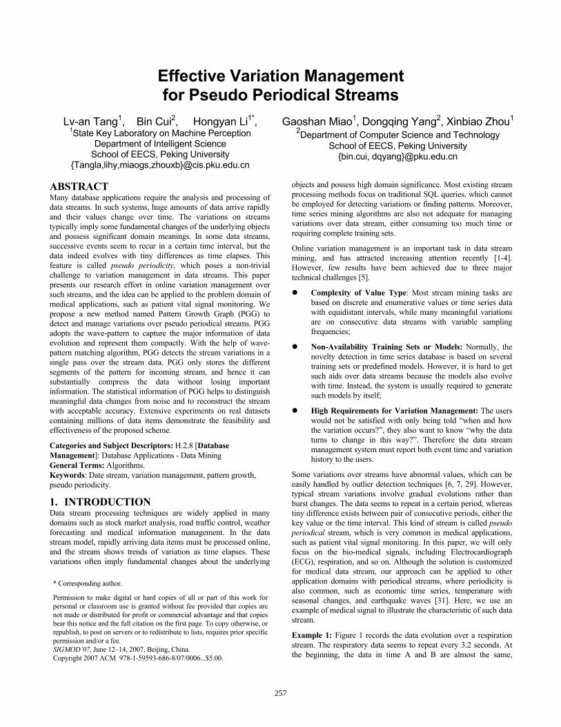
Based on the above points, we illustrate our proposed system framework in Figure 3. We split the oncoming stream into segments which are represented by wave-patterns. We compare each new wave with the previous records in PGG, and update PGG according to new pattern types. With the help of PGG, we can provide different functions, such as stream reconstruction, emergency alarm and so on.

0

1

2

3

4

5

6

0

1

2

3

4

5

6

Wave-Pattern Matching

Full Matched Increase

Frequency

Partially Matched Grow Pattern

New PatternUnmatched

OutPut

Wave Stream

Pattern Growth Graph

Wave Splitting

Online Variation Management

Online Update

Stream View

Pattern Evolutions

Data Stream

Send Alarms

Figure 3. System Framework for Variation Management

3.2 Wave Splitting Variations are detected by comparing old data with new values, and traditionally this can be done by matching stored sequences with incoming stream. However, the time and space cost are high for using such algorithms over pseudo periodical streams. First, most algorithms compare given sequences with query stream for every incoming point. It costs too much time and even causes system to collapse when huge amounts of data arrive in a short period of time; Second, since the whole sequences are stored in memory, the performance of the system will degrade when more new sequences are discovered from the stream.

If the system can divide the stream into sections and conduct the comparison between them, the time efficiency will increase substantially. However, due to the pseudo periodical effects, simply dividing the stream in fixed length will accumulate error. Hence, the first problem that we have to address is how to split a long pseudo periodical stream effectively. A careful study reveals the following observations:

Observation 1: Pseudo periodical streams are composed of waves with various time lengths and key values. The waves start and end at valley points that are less than a certain value.

Thus we can divide the stream into segments at the valley points. Generally, the upper bound value of the valley points can be specified by users in real stream applications. For example, in the

arterial blood pressure stream, the value of valley point is usually less than 50 mmHg. However, the upper bound value may change as the stream evolves. In our system, we can automatically update it using the average value of the past valley points.

NVUN

iib /)(

1∑=

=α

Where N is the number of past valley points and α is an adjustment factor to deal with outliers, and its value depends on the evolution of the stream data. The use of α can improve the flexibility of the algorithm, as the value of stream might have tiny change. However, the value ofα should be carefully selected, e.g. if it is too small, the value may generate too many false-positive alarms, while a large α may cause more false-negatives. The optimal value of α is domain-specific, and usually determined by the domain experts. For example, in ECG monitoring, α =1.1 yields the best split effect.

Another issue concerns the valley sections. If the waves are separated by long and approximately flat sections whose values are all less than the upper bound, there may be a high degree of variation in the choice of split valley points. In our approach, we always select the last valley point to split the wave, even if there are multiple valley points and the previous valley point is lower. However, if the flat section is too long, the stream is no longer pseudo periodical and the split algorithm will stop and will send an alarm.

In the implementation, we utilize a variable-length buffer to record each wave. The variation monitoring algorithm is applied on each wave.

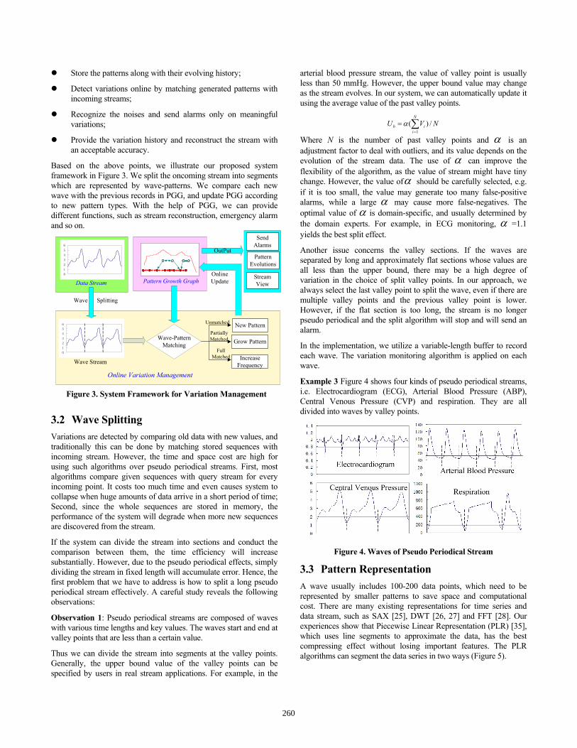
Example 3 Figure 4 shows four kinds of pseudo periodical streams, i.e. Electrocardiogram (ECG), Arterial Blood Pressure (ABP), Central Venous Pressure (CVP) and respiration. They are all divided into waves by valley points.

Figure 4. Waves of Pseudo Periodical Stream

3.3 Pattern Representation A wave usually includes 100-200 data points, which need to be represented by smaller patterns to save space and computational cost. There are many existing representations for time series and data stream, such as SAX [25], DWT [26, 27] and FFT [28]. Our experiences show that Piecewise Linear Representation (PLR) [35], which uses line segments to approximate the data, has the best compressing effect without losing important features. The PLR algorithms can segment the data series in two ways (Figure 5).

260

Figure 5. Two Different PLR Representations

PLRE: Given a data series T, produce the best linear representation such that the maximum error for any segment does not exceed the user specified threshold;

PLRK: Given a data series T, produce the best linear representation using predefined number of segments K.

Normally, the linear representation is generated in PLRE style, because the residual error is typically the main concern. But in some special case, PLRK is preferred if the users define K. To generate the PLR of segments, there exist two mechanisms. 1) Sliding window: the algorithm merges the data points along the stream, when the sum of residual error exceeds the predefined threshold, a new segment will be created; 2) Bottom up: the algorithm begins by creating the finest possible approximation of the data series, and then iteratively merges the lowest cost pair until a stopping criteria is met. In [34], an in-depth study was conducted on the two algorithms, the results showed that the time efficiency of the sliding window approach is better than the bottom up approach, but the quality is usually poor. The author mixed the advantages of them and proposed a new algorithm Sliding Window And Bottom-up (SWAB) [34], which runs as fast as Sliding window but produces high quality approximations of the data. Taking into account the cost and accuracy, we implement SWAB to simplify the wave. In our experiments, SWAB can reduce the data size to 20% with relative error bound of 5%.

Note that, if we only keep the valley and peak points, then it is equivalent to the result of simplifying the data stream using the Zigzag model [29], which may cause much larger error.

3.4 Wave-pattern Matching With the old data represented as patterns, the central issue is how to compare an incoming wave with an existing pattern to detect variations?

Traditional matching algorithm compares two sequences by calculating the value differences between data items at the same time point. It is hard for them to compare two sequences with different lengths, because one sequence may have no data item at a certain time point while the other has.

In real applications, two sequences are assumed to match if their paths roughly coincide. The PLR patterns just record paths of old data, so the variations can be detected by testing whether the incoming streams match the recorded patterns. We can determine the intensity of variation by the matching line segments in the patterns. The ideas are formalized by the following definitions:

Definition 1 (Segment Matching) Let stream subsequence L = {(X1,t1), (X2,t2), ..., (Xm, tm)}, segment Seg is the set of pairs {(X, t) with X=at+b}; Given relative error bound Eb, we say that Seg matches L if (Length (L) – Length(Seg))/Length (L) < Eb and for each i∈[1,m], Erri = |(Xi-ati-b)/Xi | ≤ Eb, where length() is a function to calculate the time duration of a sequence/segment.

Definition 2 (Wave-Pattern Matching) Let wave W = {(X1,t1), (X2,t2), ..., (Xn, tn)}, pattern P = {Seg1, Seg2, ... Segk } and Eb be the relative error bound. Suppose that W can be split into a series of continuous subsequences such that W = {L1, L2, ..., Lk},

(1) If for each i ∈[1,k], Segi matches Li, we say that P fully matches W; (2) If only j (j<k) segments match, we say that P partially matches W; (3) If no segment matches, we say that P totally un-matches W.

Example 4 Two cases of wave-pattern matching on ECG stream are shown in Figure 6. In 6(a), the pattern consists of 9 segments with time length 1.5 seconds. And the wave size is 185 points with time length 1.48 seconds. Although the sizes vary a lot, they still match according to definition 2. In 6(b), the wave and pattern partially match on segments 1, 2, 3 and 7.

0 0.5 1.0 1.5 0 0.5 1.0 1.5

Time (s) Time (s)

ECG

Figure 6. Wave-Pattern Matching

With the above definitions, the problem of wave-pattern matching transforms to the problem of splitting the wave into appropriate subsequences (segments). That is, the system must know which data points are going to be involved in a certain segment. There is a total of )k)!*k!-1-/((m1)!-(m1 =−

kmC different ways of splitting a

wave with m items into k subsequences. Therefore, it is not feasible to try all of them in data stream environment. Fortunately, the matched waves have similar PLR pattern to the old ones. Such similarity can be used to help splitting the waves as described in the following theorem.

Theorem 1: Let wave W={(X1,t1), (X2,t2), ..., (Xm, tm)}, pattern P = {Seg1, Seg2, ... Segk} and Eb is the given relative error bound, P fully matches W if the following three conditions hold: 1. W can be simplified by PLRK to a k-size pattern P’ = {Seg1’,

Seg2’, .. Segk’}, and the relative error bound is Eb1;

2. The relative difference between P’ and P is less than Eb2;

3. Eb1 + Eb2 + Eb1*Eb2 <Eb;

Proof: Since the difference between P’ and P is less than Eb2; hence for each i ∈[1,k], ||Segi - Segi’ ||/|| Segi || < Eb2 ; where

(1- Eb2) Segi < Segi’ <(1+ Eb2) Segi ... ...(1) Suppose W was split into W= {L1, L2, ... Lk } under Eb1; Thus for each i ∈[1,k], || Segi’ - Li || /|| Segi’||< Eb1; where

(1 - Eb1) Segi’ < Li <(1+ Eb1) Segi’ ... ...(2) Combine (1) and (2), we deduce that (1- Eb1)(1- Eb2)Segi < Li < (1+ Eb1)(1+ Eb2) Segi;

261

Note that Eb1>0, Eb2>0, hence the above formula can be simplified to ||Li- Segi || < Eb1+ Eb2+ Eb1* Eb2. Therefore, if Eb1+ Eb2+ Eb1* Eb2 < Eb then ||Li- Segi || < Eb; by definition 2, P matches W. According to Theorem 1, a heuristic algorithm is designed for wave-pattern matching.

Algorithm 1 Wave-pattern Matching

Input: wave W, pattern P with k segments, error bound Eb

Output: double pattern-match-error;

1． pattern P’ PLRK W with k segments. 2． Eb1 calculate error between W and P’; 3． Eb2 calculate difference between P and P’; 4． if Eb1+ Eb2+Eb1*Eb2<Eb // full match 5． then pattern-match-error Eb1+ Eb2+Eb1*Eb2; 6． else // partially match or un-match 7． split W by the points of P’; 8． for each segment S of P, do 9． match S with corresponding section of W; 10． pattern-match-error += segment match error; 11． end for 12． return pattern-match-error; After generating the PLR representation with K segments, we calculate the errors (lines 1-3). If the match error is less than the error bound, W fully matches P (lines 4-5), otherwise we need to compare the sections of W with each segment in the pattern to calculate match error (lines 6-11).

Proposition 1 Let m be the wave size and k be the pattern size, Algorithm 1’s time complexity is O(m).

Proof: The major time consumption of the algorithm is for the PLR simplification at line 1 and the matching process from line 7 to 10, both of them are O(m). The time complexity of error and difference calculation is O(k). Since k is far less than m, the total time complexity is O(m).

3.5 Pattern Growth Graph Most variations of a data stream are gradual evolutions rather than burst mutations, and many patterns just have partial segments changed. Recording all of them in a pattern list not only ignores their relationship but also causes storage redundancy. To alleviate this problem, a novel data structure Pattern Growth Graph (PGG) is designed to store patterns and their variation history.

3.5.1 Recording Variation History Each pattern in PGG is stored as a bi-directional linked list with a header node that records the pattern information, including pattern ID, frequency and the time of each occurrence of this pattern. Each brand new pattern of PGG is called base pattern. It stores the overall features of corresponding wave. All of the pattern’s segments are recorded as nodes of the bi-directional linked list. The left and right pointers of each node point to previous and next segments respectively. Three possible cases arise when we match the base pattern with an incoming wave:

Un-matched: a new base pattern will be generated and added to PGG;

Partially matched: the matched parts will be reused and new segments are generated only on un-matched data. The new

pattern grows from an old one, and we name it growth pattern;

Totally matched: there is no need to generate any new pattern, and we only increase the frequency of matched pattern and record the time of appearance.

In this way, PGG not only reduces the amount of storage requirement, but also maintains the variation history by recording the pattern growth. The pattern growth algorithm is presented as the following:

Algorithm 2 Pattern Growth over Stream

Input: stream S, pattern growth graph PGG, error bound Eb;

Output: updated pattern growth graph;

Interior variables: pattern best-match, double min-error;

1． for each incoming wave W of the stream S, do 2． Initialize best-match, min-error; 3． for each pattern P of PGG, do 4． match error Wave-pattern Matching(W, P); //Algo.1 5． if match error < Eb then 6． increase the pattern P’s frequency; 7． break; // totally matched, no more comparison 8． else if match error < min-error then 9． best-match P; // record the best match pattern 10． min-error match error; 11． end for 12． if best-match is null then // totally un-matched 13． generate new base pattern P’; 14． add P’ to PGG; 15． else if min-error > Eb then // partially matched 16． remove matched data from W; 17． use PLRE to generate growth pattern P’ from W; 18． update P’s each node left and right pointers; 19． add P’ to PGG; 20． Record the occurrence time of the pattern; 21． end for 22． return PGG. Proposition 2 Let n be the number of waves in the data stream and k be the number of patterns in a PGG, the time complexity of Algorithm 2 is O(n2). In the worst case, Algorithm 2 needs to compare every stream wave with each pattern in PGG, and each incoming wave introduces a new pattern, so the overall time cost is k + (k+1) + (k+2) +...+ (k+n-1) = k*n + n*(n-1)/2. Note that, the comparison could be stopped once a full matched pattern has been found and the majority of waves appear repeatedly in pseudo periodical streams. Therefore, the time cost is much smaller in real applications. The proof is straightforward, so we omit the details. Example 5 In Figure 7, pattern 1 is a base pattern with eight segments. It partially matches the new stream wave on segment 1, 2, 3 and 7. Therefore, a growth pattern (pattern 2) with segments 1’--4’ is generated based on the un-matched data. The left pointer of segment 1’ points to the previous segment - segment 3, and the right pointer of segment 2’ points to the next segment - segment 7.

262

Figure 7. Pattern Growth Graph

3.5.2 Construct Full Wave-pattern Using Growth Patterns Intuitively, the storage cost can be reduced by only storing the variant parts of patterns. However, a new problem arises: the wave-pattern matching needs to compare incoming wave with every pattern in an online fashion – which requires that the pattern to be compared with must be a full pattern. Therefore the system needs to be able to generate a full pattern from growth patterns as fast as it accesses a base pattern. This process can be completed by propagating the pointers of nodes in growth patterns. The details are presented in Algorithm 3.

Algorithm 3 Construct Wave-pattern Using Growth Patterns

Input: pattern growth graph PGG, growth pattern P’;

Output: corresponding full pattern P;

Interior variables: pointer array LP and RP;

1． add the nodes of P’ to P; 2． for each node N of P’, do 3． add N’s left pointers to LP; 4． add N’s right pointers to RP; 5． end for 6． while (there exist active pointers in LP or RP),do 7． for each active pointer LP[j] and RP[i] , do 8． add the node NL pointed by LP[j] to P; 9． LP[j] NL’s left pointer; 10． add the node NR pointed by RP[i] to P; 11． RP[i] NR’s right pointer; 12． if LP[j] = “Start” then deactivate LP[j]; 13． if RP[i] = “End” then deactivate RP[i]; 14． if (i = j-1 & LP[j] <= RP[i]) then //pointers collide 15． deactivate LP[j] and RP[i]; 16． end for 17． end while 18． return P. In this algorithm, we first put each node’s left pointer in LP and right pointer in RP (lines 2-4). In line 6, we check whether there are active pointers in LP or RP (the original statuses of the pointers are all active.). Then, we access the active pointers in two pointer arrays and add the reused nodes into P by propagating pointers (lines 7-11). The active pointers are deactivated under three circumstances: 1. the left pointer moves to “Start” sign (line 12); 2. the right pointer moves to “End” sign (line 13); 3. two pointers collide together (lines

14-16). When all cursors stop (line 18), the full wave-pattern will be returned. A new example is used to better illustrate the process of Algorithm 3.

Example 6 Figure 8 shows the process of computing growth pattern 3 by propagating pointers. At the beginning, only the new nodes 1” and 2” can be read by pattern’s ID (line 1 of Algorithm 3). Four pointers LP1, RP1, LP2 and RP2 are generated (line 2-5). In propagating step 1, the nodes pointed by these pointers, 1’, 2’ and 9, are added (line 8-11). Pointer RP2 reaches the end sign of the pattern (line 13). In step 2, nodes 1, 3’, 8 are added; and in the final step, pointer LP1 reaches the start sign (line 12), and pointer LP2 and RP1 collide at node 8 (line 14-15). When all pointers stop, the algorithm outputs the final result (line 18).

Figure 8. Construct Full Wave-pattern

Proposition 3 Let m be the size of a growth pattern, n be the size of a whole pattern, Algorithm 3 costs O(m) space and the time complexity is O(m+log2m(n-m)).

Proof: The only extra space needed by the algorithm is to store two m-size pointer arrays. The time to compute the whole pattern is to get n-m nodes via 2m pointers. Thus the time complexity is O(m+ log2m(n-m)).

With a little space overhead, the time cost of growth pattern access is even better than reading base pattern directly.

3.5.3 Rank the Patterns Proposition 2 shows that the time complexity for pattern growth is O(n2). When PGG becomes larger, comparing the incoming wave with PGG’s patterns one by one is still very time-consuming. Online learning algorithms traditionally use “a forgetting function” to get rid of the historical data’s influence. However, PGG cannot adopt traditional forgetting policies to delete old patterns. After a careful study on matching patterns we find the following:

Observation 2 The most frequent pattern and its similar patterns (all the patterns which have the same base pattern) have the highest possibilities to match the incoming wave.

Thus, we can rank the patterns by their matching frequency and the performances of their “families”. Let N be the count of pattern frequency, M be the number of its similar patterns, △Xi be the recorded error value of each match, ti be the time point of each matching, ds be the distance between two patterns, we design a matching probability factor for pattern p at time point t as follows:

)*exp()*exp(t)(N,F111∑∑∑===

Δ−+Δ−=jN

jii

M

ij

N

iii XWSXW

263

Where the time factor )/1( ttW ii −= , and the similarity factor

∑ −−= =Mk jkjj ppdsppdsS 1 )](/)(exp[ .

This function integrates multiple factors which affect the matching probability of a known pattern including frequency, match error, previous match time and pattern family. For example, the matching probability of a pattern decreases if the match error becomes larger or no new incoming wave matches the pattern. The exp() function helps to amplify the effect of latest matched patterns, because there are typically gradual evolutions in pseudo periodical streams. An index is constructed according to matching possibilities. Although the patterns with smaller probability cannot be deleted, they have lower priority to be compared. In addition, if one pattern matches the wave, the system will not only increase its own frequency, but also increase the rank of its “families”. In this way, even in the worst case, the time complexity is still O(n2). Our experiments show that the average speed will increase about 20% -- 300% as the stream passes by.

4. APPLICATIONS OF VARIATION MANAGEMENT Pattern Growth Graph keeps track of data features and variation history of pseudo periodical streams, which are very useful for user’s future study. Here, we introduce three typical applications of PGG.

4.1 Maintain the Pattern Evolution Variation management requires the system to report both the event time and the history of pattern evolution. With the PGG structure, we store the segment patterns of the data stream in a compressed format. We can also generate the full pattern using the reconstruction algorithm. When a user selects a set of interesting patterns, the system can track the source of them by propagating their pointer arrays. The base pattern records the initial state, and various growth patterns reflect its evolutions over the data stream. Additionally, the system can give the first occurring time for each pattern, either the base pattern or the growth pattern. (Figure 9)

Figure 9. Track Pattern’s Evolutions

PGG also provides the perspective for single pattern family. A base pattern can be seen as the root node of a pattern family tree, the growth patterns are the child nodes, and the PGG is a forest for such trees.

4.2 Reconstruct the Stream View Queries on traditional data stream systems need to be predefined, so it is hard to conduct queries on the historic data since they have passed by. All patterns’ occurrence time points have been recorded in the PGG. If a user wants to know a general situation such as “the patient's ECG in the past five hours”, the system can search the patterns within this period and reconstruct an approximate stream view. Because the patterns are generated strictly under the maximum error bound, the stream view has the same precision. Normally storing the patterns’ occurrence times in a PGG only consumes about 3% storage space of the original stream, but it can provide an approximate stream view within 5% relative error bound, achieving excellent compression effects.

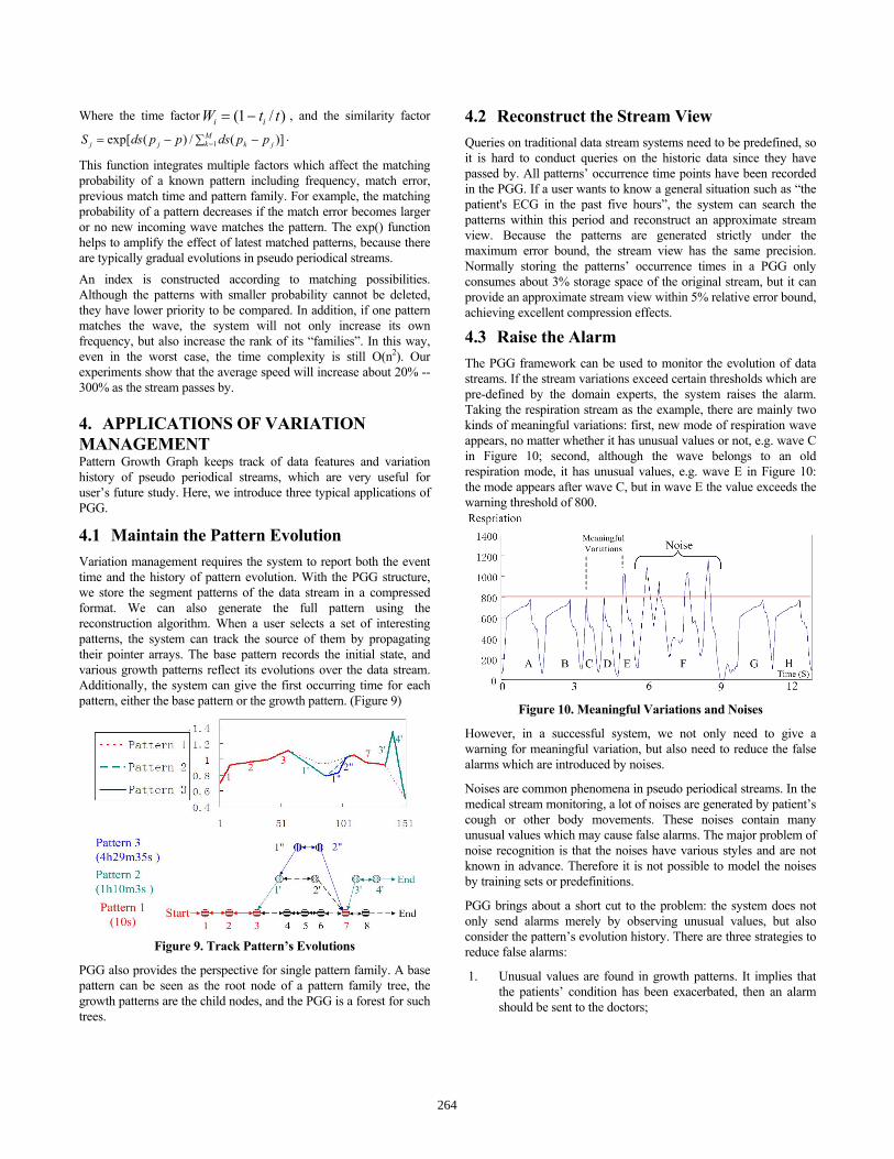
4.3 Raise the Alarm The PGG framework can be used to monitor the evolution of data streams. If the stream variations exceed certain thresholds which are pre-defined by the domain experts, the system raises the alarm. Taking the respiration stream as the example, there are mainly two kinds of meaningful variations: first, new mode of respiration wave appears, no matter whether it has unusual values or not, e.g. wave C in Figure 10; second, although the wave belongs to an old respiration mode, it has unusual values, e.g. wave E in Figure 10: the mode appears after wave C, but in wave E the value exceeds the warning threshold of 800.

Figure 10. Meaningful Variations and Noises

However, in a successful system, we not only need to give a warning for meaningful variation, but also need to reduce the false alarms which are introduced by noises.

Noises are common phenomena in pseudo periodical streams. In the medical stream monitoring, a lot of noises are generated by patient’s cough or other body movements. These noises contain many unusual values which may cause false alarms. The major problem of noise recognition is that the noises have various styles and are not known in advance. Therefore it is not possible to model the noises by training sets or predefinitions.

PGG brings about a short cut to the problem: the system does not only send alarms merely by observing unusual values, but also consider the pattern’s evolution history. There are three strategies to reduce false alarms:

1. Unusual values are found in growth patterns. It implies that the patients’ condition has been exacerbated, then an alarm should be sent to the doctors;

264

2. A new base pattern is generated, and it matches or partially matches successive waves. This phenomenon means that the underlying pathology mechanism might have some fundamental changes. Although the new pattern may not contain unusual values, the alarm will also be sent out;

3. A series of new base patterns are generated continually, and they all un-match the following waves. These incoming waves can be simply classified as noises.

In the practical applications, the final judge and noise deletion still depend on professional doctors, and the system just adds suspicion tags to facilitate their judgments.

5. EXPERIMENTAL RESULTS In this section, a thorough experimental study on PGG is conducted. First we evaluate some factors that affect the performance of proposed PGG; then we compare it with some existing techniques; followed by a short discussion.

5.1 Experimental Setup As the idea is motivated by application problems, we used real datasets instead of synthetic ones. Three kinds of pseudo periodical streams are used in the experiments: 1. Medical streams: Six real pathology signals including ECG,

respiration, pulse oxymetry (PLETH) are recorded during a six hour period simultaneously from a pediatric patient with traumatic brain injury. The sample rates of the signals are from 125 Hz to 500 Hz, varying according to the states of illness. The whole dataset includes over 25,000,000 data points;

2. Earthquake waves [36]: The pacific earthquake wave data is downloaded from the NGA project at the Pacific Earthquake Engineering Research Center at UC Berkeley. The sample rates are from 500Hz to 1000Hz. The data size is about 100,000 data points;

3. Sunspot data [37]: Provided by the national schools' observatory of UK, the dataset includes all the sunspot records between the year 1850 and 2001, and it contains about 55,000 data points. It is not a strict stream due to the long time range, but the data is also pseudo periodical.

The above datasets are produced by different equipments or sensors using multiple formats. The value ranges and data units vary a lot in different sources. So we use relative error percentage as error bound for pattern generation and matching in the experiments.

For performance evaluation metric, we use the processing efficiency, the effectiveness in variation detection and noise recognition. Traditionally, two important measurements are used in detecting variations.

Sensitivity (High Positive Rate): The probability that the algorithm can find meaningful variations in a data stream;

Selectivity (Low Negative Rate): The probability that the algorithm does not send false alarms on noises.

The two measurements are conflict in a sense that increasing sensitivity to find more variations will inevitably cause more false alarms, i.e. the lower selectivity.

The experiments were conducted on an Intel Pentium 4 3.0GHz CPU with 1GB RAM, and the experimental environment is Windows XP Professional, JDK 1.5.0.

5.2 Performance on PGG 5.2.1 Effectiveness of the Rank Function As we introduced in section 3.5.3, PGG needs to examine all the existing patterns to match the incoming stream. The naive approach is to scan the patterns sequentially. However, we notice that the frequent patterns have higher probability to be matched. The first experiment is to test the effectiveness of the rank function, which sorts the patterns in PGG according to their frequencies. The experiment was carried out on the largest ECG dataset with 10,803,200 data points. The numbers of data points processed per second, with and without the pattern ranking function, are recorded in Figure 11. The performances decrease when more streams come, as both approaches need to examine the stored patterns for pattern match and update. The incoming streams inevitably increase the number of stored patterns. At the beginning, the effect of pattern ranking is insignificant. But after three million data points, when more patterns are generated, the naive algorithm’s performance decreases rapidly. In the end, the rank algorithm outperforms the original algorithm by about 300%.

Figure 11. Ranked vs Sequential Scan Results

Figure 12. Numbers of Patterns

5.2.2 Pattern Evolution Figure 12 records the numbers of base patterns and growth patterns under a 3% relative error bound. As expected, more than 70% of the patterns are evolved from the rest 30% patterns. Another interesting discovery is that among the six medical streams, the numbers of growth patterns increase with the stream size, while the numbers of base patterns are nearly the same. Moreover, we can use a relatively small number of patterns to represent a long data stream, e.g. ECG dataset has more than 10M data points, which can be represented with only 420 patterns using the PGG.

265

5.2.3 Space Cost We also carried out experiments on the space cost of PGG. Note that, the space cost includes the information of frequency of patterns and every occurrence time of patterns, which is essential to reconstruct stream view. Figure 13 shows the space costs of PGG with different error thresholds in reconstructing the ECG stream. PGG can achieve over 95% accuracy with a storage cost that is less than 4% of the original stream. This amazing result is achieved due to two factors. The SWAB can reduce the size of patterns to about 20% of the original size, and PGG further reduces it to 3% by compressing the repeating and similar patterns. In this 3.31% storage cost, PGG itself only needs 0.3%, the rest 3% stores the occurrence time of the patterns – which must be recorded for stream reconstruction and almost impossible to be compressed.

Figure 13. Storage Cost of PGG

Figure 14. Online Updating vs Training Testing

5.2.4 Pattern Update Another problem we consider is whether it is necessary for PGG to update patterns for all incoming streams. An experiment was designed to compare the Online Updating (OU) style with Training-Testing (TT) style. We asked three professional doctors to tag out 278 meaningful variations and 97 noise sections on the respiration stream with 2,700,200 points. In TT, we only generated the PGG using the training data stream, e.g. the first 320,000 points (about 11%) of the stream are employed as the training set in this experiment. Figure 14 shows the results obtained under 5% relative error threshold. In both styles, the ratios of the false alarms are almost the same, but the training-testing style’s sensitivity decreases when more stream data comes. If no new pattern is added, the algorithm cannot figure out whether the new variation is meaningful or just a noise, and hence may ignore it and do not send any alarm.

5.3 Comparison with Other Methods We compared PGG with three most relevant methods, i.e. SAX (symbolic approaches) [25], Discrete Haar Wavelet Transformation (mathematic transformation) [27], Zigzag (predefined models) [29]. PGG only needs the user to define a relative error bound, while some other algorithms require the user to define a window. Because the Haar DWT algorithm typically operates the data using the lengths with power of 2, we used a 1024 fixed-size window if necessary. The DWT algorithm can be only applied on time series in fixed sampling frequency and most of the above datasets do not satisfy this condition. We have to choose such sub-sequences from original datasets for DWT. The size of that chosen sets is about 5% of the original data. All the algorithms are implemented in Java on Eclipse 3.2.2.

5.3.1 Processing Efficiency The first experiment is about processing efficiency. The four algorithms were compared on all the eight pseudo periodical streams. The average numbers of data points processed per second are recorded in Figure 15.

Figure 15. Results on Process Efficiency

The results show that Zigzag yields the best performance. The reason is that the Zigzag model only records and compares the extreme values. All algorithms perform worst on the ECG stream, as ECG has the largest size and the maximum number of variations. However, even the worst algorithm (DWT on ECG) can handle over 10,000 points per second, much higher than what the real applications require. With better hardware environment, the performance can be further improved.

5.3.2 Variation Detection and Noise Recognition This experiment was carried out on respiration stream. It is the only dataset with fixed sampling frequency (125 data points per second), so that DWT can run on the whole stream. As described in 5.2.4, 278 meaningful variations and 97 noise sections are tagged on the stream. Since both selectivity and sensitivity are strongly influenced by the parameters, we carried out the experiments with different thresholds. In an ICU environment, missing a meaningful variation may cost the patient’s life, so sensitivity is much more important than selectivity. Figure 16 shows the performances of the four algorithms on detecting meaningful variations, along with the numbers of their false alarms.

266

Figure 16. Results on Effectiveness

The result indicates that the Zigzag based algorithm, with the highest time efficiency, has difficulty finding out meaningful variations. Instead it sends false alarm at almost every noise section. This behavior is caused by the characteristic of the Zigzag model. It only compares the extreme points, while most noises have outliers with very high or low values. The DWT and SAX methods also perform poorly. They miss over 25% meaningful variations but send about 70% false alarms, indicating that they nearly cannot make distinction between real variations and noises. The PGG approach performs the best. It finds out all the variations with only 12 false alarms. Manually tagging all meaningful variations and noises in a long stream is a heavy burden for a human being and is not feasible in our comparison. So in the experiments on other datasets, we take precision as the main measurement. The three algorithms (DWT doesn’t work any more) found out 50 variations on each dataset. And a professional doctor examined the result, judged whether they are meaningful variations or just false alarms. The results are reported in Figure 17.

Figure 17. Precision on Detected Variations

The results show that PGG performs accurately and stably over all datasets, while the performance of Zigzag is volatile with different datasets. Three blood pressure signals (ABP, CVP and ICP) are seldom influenced by patient’s movements, and most of their variations appear due to unusual extreme values, and hence Zigzag’s accuracy is high. However, the extreme values in the PLETH stream are almost the same, and the meaningful variations are mainly due to the changes of inner structures. Therfore Zigzag almost cannot work properly in the latter case.

5.4 Discussion Why do the competitors perform poorly in variation detection on pseudo periodical stream?

1. The main drawback of Zigzag is that it only focuses on extreme data points. It may work well on some zigzag style streams like blood signals or stock market data, but on other streams, the results will be strongly influenced even by one or two outliers.

2. SAX is a kind of statistical algorithm, which needs large training dataset to be effective. SAX is good at finding novelty or surprising patterns in a long period using frequency statistics, but it lacks the power to detect inner changes of shorter waves instantly. The experiments indicate that it is more suitable for time series mining than data stream management.

3. The mathematical transformation methods, such as DWT and FFT, are effective for fixed-size data patterns, especially for the signals with strict periods, whereas data stream’s pseudo-periodicity greatly reduces their accuracy.

Then why does PGG work well in the experiments?

PGG captures the main features of pseudo periodical data streams: (1) most waves are structurally similar with tiny difference in details; and (2) the variations are gradual evolutions rather than mutations. The wave-pattern matching algorithm is not strict on point variations, but it seeks common ground while preserving structural differences. Thus, PGG is capable of finding the variations that other algorithms may ignore. In addition, PGG not only stores new patterns, but also records their variation history. The recorded pattern history provides sufficient information to help distinguish between meaningful variations and noises. In other word, with the effective data structure, PGG discovers and records as much features of the data stream as possible.

6. CONCLUSION In this paper, we addressed the problem of variation management for pseudo periodical streams. Upon studying real-time application requirements, we proposed a new Pattern Growth Graph (PGG) based method for variation detection management, and history recording. In PGG, the streams are represented by wave-patterns efficiently. We proposed to detect the stream variation using pattern matching algorithm in a single pass over data, and store the variation history with small storage overhead. PGG can effectively distinguish meaningful variations from noise, and reconstruct the stream view within an acceptable accuracy. Extensive experiments have been conducted to show the superiority of the PGG variation management for pseudo periodical streams.

In the near future, we plan to extend PGG to multiple streams monitoring and to implement the PGG method in other application domains such as weather forecasting and financial analysis.

7. ACKNOWLEDGMENTS The authors would like to thank Jiawei Han, Yuqing Wu, Shiwei Tang for their helpful discussion and comments on the research carried out in this paper; Haibin Liu, Huiguan Ma, Chi Zhang, Yu Fan, Zijing Hu and Jianlong Gao for system implementation; and the anonymous reviewers for their feed back. The work described in this paper was supported by NSFC under grant number 60673113.

267

8. REFERENCES [1] Spiros Papadimitriou, Philip S. Yu: Optimal Multi-Scale

Patterns in Time Series Streams, In SIGMOD 2006. [2] Charu C. Aggarwal, Jiawei Han, Jianyong Wang, Philip S. Yu:

A Framework for Projected Clustering of High Dimensional Data Streams, In VLDB 2004.

[3] Haixun Wang, Wei Fan, Philip S. Yu, Jiawei Han. Mining Concept Drifting Data Streams using Ensemble Classifiers. In SIGKDD 2003.

[4] Brian Babcock, Mayur Datar, Rajeev Motwani, Liadan O’Callaghan: Maintaining variance and k-medians over data stream windows. In PODS 2003.

[5] Jian Pei, Haixun Wang and Philip.S.Yu: Online Mining Data Streams: Problems, Applications and Progress. In ICDE 2005.

[6] Eamonn J. Keogh, Jessica Lin, Ada Wai-Chee Fu: HOT SAX: Efficiently Finding the Most Unusual Time Series Subsequence. In ICDM 2005.

[7] Eamonn J. Keogh, Stefano Lonardi, Bill Yuan-chi Chiu: Finding surprising patterns in a time series database in linear time and space. In SIGKDD 2002.

[8] Spiros Papadimitriou, Jimeng Sun, Christos Faloutsos: Streaming Pattern Discovery in Multiple Time-Series. In VLDB 2005.

[9] Shivnath Babu and Jennifer Widom: Continuous Queries over Data Streams. In SIGMOD 2001.

[10] Daniel J. Abadi, Don Carney, Ugur Cetinteme, et al: Aurora: A New Model and Architecture for Data Stream Management. In VLDB Journal, August 2003.

[11] Sirish Chandrasekaran, Owen Cooper, Amol Deshpande, et al: TelegraphCQ: Continuous Dataflow Processing for an Uncertain World. In CIDR 2003.

[12] Yong Yao, Johannes Gehrke: The Cougar Approach to In-Network Query Processing in Sensor Networks. SIGMOD Record, 31(3). September 2002.

[13] Babcock Brian, Datar Mayur and Motwani Rajeev: Sampling from a moving window over streaming data. In SODA, 2002.

[14] Graham Cormode, Mayur Datar, Piotr Indyk, S. Muthukrishnan: Comparing data streams using hamming norms. In VLDB, 2002.

[15] Mayur Datar, Aristides Gionis, Piotr Indyk and Bajeev Motwani. Maintaining stream statistics over sliding windows. In SODA, 2002.

[16] Sumit Ganguly, Minos Garofalakis and Rajeev Rastogi: Processing set expressions over continuous update streams. In SIGMOD, 2003.

[17] Wong David, Gallegos Yvonne, Weinger Matthew, et al: Changes in intensive care unit nurse task activity after installation of third-generation intensive care unit information system. Crit Care Medi, 2002, 31.

[18] David J. Fraenkel, Melleesa Cowie, Peter Daley: Quality benefits of an intensive care clinical information system. Crit Care Medi, 2003, 31.

[19] Varon Joseph, Marik PE: Clinical information systems and the electronic medical record in the intensive care unit. Current Option in Critical Care. 2002, 8(6), 616-624

[20] Y. Dora Cai, David Clutter, et al: MAIDS: Mining Alarming Incidents from Data Streams, In SIGMOD 2004.

[21] WeiGuang Teng, MingSyan Chen, Philip S. Yu. A regression-based temporal pattern mining scheme for data streams. In VLDB 2003.

[22] Yunyue Zhu, Dennis Shasha: Efficient elastic burst detection in data streams. In SIGKDD 2003

[23] Junshui Ma and Simon Perkins: Online novelty detection on temporal sequences. In SIGKDD 2003.

[24] Charu C. Aggarwal: On Abnormality Detection in Spuriously Populated Data Streams. In ACM SIAM 2005

[25] Jessica Lin, Eamonn Keogh, Stefano Lonardi, Bill Chiu: A symbolic representation of time series, with implications for streaming algorithms. In DMKD 2003.

[26] Anna C. Gilbert, Yannis Kotidis, S. Muthukrishnan and Martin J. Strauss: One-Pass Wavelet Decompositions of Data Streams. IEEE Trans. Knowl. Data Eng. 15(3), 2003.

[27] Spiros Papadimitriou, Anthony Brockwell and Christos Faloutsos: Adaptive, unsupervised stream mining. VLDB Journal 13(3), 2004.

[28] Like Gao, Xiaoyang Sean Wang: Continuous Similarity-Based Queries on Streaming Time Series. IEEE Trans. Knowl. Data Eng. 17(10) 2005.

[29] Huanmei Wu, Betty Salzberg, Donghui Zhang: Online Event-driven Subsequence Matching over Financial Data Streams. In SIGMOD 2004.

[30] Huanmei Wu, Gregory C Sharp, et al: A Finite State Model for Respiratory Motion Analysis in Image Guided Radiation Therapy. Phys. Med. Biol., 2004.

[31] Huanmei Wu, Betty Salzberg, Gregory C Sharp, Steve B Jiang, Hiroki Shirato, David Kaeli: Subsequence Matching on Structured Time Series Data. In SIGMOD 2005.

[32] Charu C. Aggarwal: A framework for diagnosing changes in evolving data streams. In SIGMOD 2003.

[33] Haixun Wang and Jian Pei: A Random Method for Quantifying Changing Distributions in Data Streams. In PKDD 2005.

[34] Eamonn Keogh, Selina Chu, David Hart, et al: An Online Algorithm for Segmenting Time Series. In ICDM 2001.

[35] Xiaoye Wang, Zhengou Wang: A structure-adaptive piece-wise linear segments representation for time series. In Proceedings of Information Reuse and Integration 2004.

[36] http://peer.berkeley.edu/nga/flatfile.html [37] http://www.schoolsobservatory.org

268