Journal of Development Economics 101 (2013) 92–104

Contents lists available at SciVerse ScienceDirect

Journal of Development Economics

j ourna l homepage: www.e lsev ie r .com/ locate /devec

Effective labor regulation and microeconomic flexibility☆

Ricardo J. Caballero a,b,⁎, Kevin N. Cowan c, Eduardo M.R.A. Engel b,d, Alejandro Micco e

a MIT, United Statesb NBER, United Statesc Central Bank of Chile, Chiled Yale University, United States, and University of Chile, Chilee University of Chile and Centro de Microdatos, Chile

☆ We thank Joseph Altonji, John Haltiwanger, Michaeeditor and two anonymous referees for helpful commenthe NSF for financial support.⁎ Corresponding author at: MIT. Tel.: +1 617 253 048

E-mail address: caball@mit.edu (R.J. Caballero).1 See, e.g., the review in Caballero and Hammour (202 See, e.g., Foster et al. (1998).

0304-3878/$ – see front matter © 2012 Elsevier B.V. Alhttp://dx.doi.org/10.1016/j.jdeveco.2012.08.009

a b s t r a c t

a r t i c l e i n f o

Article history:Received 13 July 2010Received in revised form 19 March 2012Accepted 31 August 2012

JEL classification:E24J23J63J64K00

Keywords:Microeconomic rigiditiesCreative-destructionJob security regulationAdjustment costsRule of law

Microeconomic flexibility is at the core of economic growth in modern market economies because it facili-tates the process of creative-destruction. The main reason why this process is not infinitely fast, is thepresence of adjustment costs, some of them technological, others institutional. Chief among the latter islabor market regulation. While few economists object to the hypothesis that labor market regulationhinders the process of creative-destruction, its empirical support is limited. In this paper we revisit this hy-pothesis, using a new sectoral panel for 60 countries and a methodology suitable for such a panel. We findthat job security regulation clearly hampers the creative-destruction process, especially in countries whereregulations are likely to be enforced. Moving from the 20th to the 80th percentile in job security, in countrieswith strong rule of law, cuts the annual speed of adjustment to shocks by a third while shaving off about 1%from annual productivity growth. The same movement has negligible effects in countries with weak rule oflaw.

© 2012 Elsevier B.V. All rights reserved.

1. Introduction

Microeconomic flexibility, by facilitating the ongoing process ofcreative-destruction, is at the core of economic growth in modern mar-ket economies. This basic idea has been with economists for centuries,was brought to the fore by Schumpeter more than fifty years ago, andhas recently been quantified in a wide variety of contexts. 1 In USmanufacturing, for example, more than half of aggregate productivitygrowth can be directly linked to this process. 2

The main obstacle faced by microeconomic flexibility is adjust-ment costs. Some of these costs are purely technological, others areinstitutional. Chief among the latter is labor market regulation, in par-ticular job security provisions. The literature on the impact of labormarket regulation on the many different economic, political and so-ciological variables associated to labor markets and their participants

l Keane, Norman Loayza, thets. Caballero and Engel thank

9; fax: +1 617 253 6915.

00).

l rights reserved.

is extensive and contentious. However, the proposition that job secu-rity provisions reduce restructuring is a point of agreement.

Despite this consensus, the empirical evidence supporting thenegative impact of labor market regulation on microeconomic flexi-bility has been scant at best. This is not too surprising, as the obstaclesto empirical success are legions, including poor measurement ofrestructuring activity and labor market institution variables, bothwithin a country and more so across countries. 3 In this paper wemake a new attempt. We develop a methodology that allows us tobring together the extensive new data set on labor market regulationconstructed by Botero et al. (2004) with comparable cross-countrycross-sectoral data on employment and output from the UNIDO

3 On a closely related literature, there is an extensive body of empirical work,pioneered by Lazear (1990), that has put together data on job security provisionsacross countries and over time, and measured the effect of these provisions on aggre-gate employment. A recent survey of this literature can be found in Heckman andPagés (2003). Results are mixed. On the one hand, Lazear (1990), Grubb and Wells(1993), Nickell (1997) and Heckman and Pages (2000) find a negative relationship be-tween job security and employment levels. On the other hand Garibaldi and Mauro(1999), OECD (1999), queryAddison et al. (2000), and Freeman (2001) fail to find ev-idence of such a relationship.

93R.J. Caballero et al. / Journal of Development Economics 101 (2013) 92–104

(2002) data-set. We also emphasize the key distinction between ef-fective and official labor market regulation.

The methodology builds on the simple partial-adjustment ideathat larger adjustment costs are reflected in slower employment ad-justment to shocks. 4 The accumulation of limited adjustment tothese shocks builds a wedge between frictionless and actual employ-ment, which is the main right hand side variable in this approach. Wepropose a new way of estimating this wedge, which allows us to pooldata on labor market legislation with comparable employment andoutput data for a broad range of countries. As a result, we are ableto enlarge the effective sample to 60 economies, more than doublethe country coverage of previous studies in this literature. 5 Our at-tempt to measure effective labor regulation interacts existing mea-sures of job security provision with measures of rule of law andgovernment efficiency. 6

Our results are clear and robust: countries with less effective jobsecurity legislation adjust more quickly to imbalances between fric-tionless and actual employment. In countries with strong rule oflaw, moving from the 20th to the 80th percentile of job securitylowers the speed of adjustment to shocks by 35% which amounts toa cut in annual productivity of 0.85% in an AK-type world. The samemovement for countries with low rule of law only reduces thespeed of adjustment by approximately 1% and productivity growthby 0.02%.

The paper proceeds as follows. Section 2 presents the methodolo-gy and describes the new data set. Section 3 discusses the main re-sults and explores their robustness. Section 4 gauges the impact ofeffective labor protection on productivity growth. Section 5 concludesand is followed by various appendices.

2. Methodology and data

Our methodology is based on an adjustment cost model wherethe dynamic employment gap is given by a simple expression in-volving employment and nominal output, both of which are avail-able in the sectoral panel for the 60 countries we use in theempirical part.

2.1. Methodology

The starting point is a partial adjustment framework where thechange in the number of (filled) jobs in sector j in country c betweentime t−1 and t is a fraction of the gap between desired and actualemployment. That is:

Δejct ¼ ψjct e�jct−ejc;t−1

� �; ð1Þ

where e and e∗ denote the logarithm of employment and desired em-ployment, respectively.

Eq. (1) can be rationalized via quadratic adjustment costs (Sargent,1978), or an exogenous process where the ψjct is either zero or one(Calvo, 1983), or a stochastic adjustment cost model that nests the pre-ceding models as particular cases (Caballero, Engel and Micco, 2004).For simplicity we consider the Calvo interpretation. We therefore as-sume that the ψjct is i.i.d., both across sectors and over time, takingvalues 0 or 1, with a country-specific mean λc. Since these stochastic

4 For surveys of the empirical literature on partial-adjustment see Nickell (1986)and Hamermesh (1993).

5 To our knowledge, the broadest cross-country study to date – Nickell and Nunziata(2000) – included 20 high income OECD countries. Other recent studies, such as Bur-gess and Knetter (1998) and Burgess et al. (2000), pool industry-level data from 7OECD economies.

6 See Loboguerrero and Panizza (2003) for a similar interaction term in a study ofthe relation between labor market institutions and inflation.

adjustment speeds can be viewed as resulting from adjustment coststhat are either zero (with probability λc) or infinite (with probability1−λc) we refer to these frictions as “adjustment costs”. The parameterλc captures microeconomic flexibility. As λc goes to one, all gaps areclosed quickly and microeconomic flexibility is maximum. As λc de-creases, microeconomic flexibility declines.

Eq. (1) hints at two important components of our methodology:We need a measure of the employment gap and a strategy to estimatethe country-specific speeds of adjustment (the λc). We describe bothingredients in detail in what follows. In a nutshell, we construct esti-mates of ejct∗ , the only unobserved element of the gap, by solving theoptimization problem of a sector's representative firm, as a functionof observables such as labor productivity and a suitable proxy forthe average market wage. We estimate λc based upon the largecross-sectional size of our sample and the well documented heteroge-neity in the realizations of the gaps (see, e.g., Caballero, Engel andHaltiwanger (1997) for US evidence).

2.1.1. Employment gap measureA sector's representative firm faces an isoelastic demand and has

access to a production technology that is Cobb–Douglas in labor andhours per worker:

y ¼ aþ αeþ βh;

p ¼ d−1ηy;

where y, p, e, h, a and d denote output, price, employment, hours perworker, productivity and demand shocks ,respectively, and η is theprice-elasticity of demand. We let γ≡(η−1)/η, and assume η>1,α>β>0 and αγb1. Firms are competitive in the labor market butpay wages that increase with hours worked according to a wageschedule w(h), with w′ and w″ strictly positive. All lower case vari-ables are in logs.

If the firm can adjust hours and employment in every period at nocost, then its profit maximizing inputs, denoted by h and e, are char-acterized by:

w′ h� �

¼ βα; ð2Þ

e ¼ 11−αγ

log βγ þ dþ γa− 1−βγð Þh−log W ′ H� �n oh i

; ð3Þ

where logW(H)≡w(logH) and logH≡h (see Appendix A for the deri-vation). It follows from Eq. (2) that our functional forms imply thatthe optimal choice of hours, h, does not depend on productivity anddemand shocks.

Having solved the problem of a firm that faces no frictions, weturn next to the case with adjustment costs. A key assumption isthat the representative firm within each sector only faces adjust-ment costs when it changes employment levels, not when it changesthe number of hours worked. 7 It follows that the sector's choice ofhours in every period can be expressed in terms of its current levelof employment, by solving the corresponding first order conditionfor hours, which leads to an expression analogous to Eq. (3) with hand e in the place of h and e. Subtracting this expression from Eq. (3)and writing the Taylor expansion for log{W′(eh)} around h ¼ h as

log W ′ Hð Þn o

≅log W ′ H� �n o

þ μ−1ð Þ h−h� �

;

7 For evidence on this see Sargent (1978) and Shapiro (1986). Also note that over-time payments, captured by the wage schedule w(h), should not be viewed as adjust-ment costs since they depend on the level of hours worked, not on the change in hours.

94 R.J. Caballero et al. / Journal of Development Economics 101 (2013) 92–104

with μ−1≡W″ H� �

H=W ′ H� �

assumed positive, we obtain: 8

e−e ¼ μ−βγ1−αγ

h−h� �

: ð4Þ

This is the expression used by Caballero and Engel (1993). It can-not be applied in our case, since we do not have information on hoursworked. For this reason we derive next an analogous expression relat-ing the employment gap to the labor productivity gap; as we discusslater in this section, we have the data to apply this expression.

The value of the marginal product of labor (referred to, with someabuse, as “marginal labor productivity” in what follows) satisfies:

v ¼ log αγ þ dþ γa− 1−αγð Þeþ βγh:

Subtracting this expression from its frictionless counterpart (obtainedby substituting h and e for e and h) and then using Eq. (4) to get rid of thehours gap yield:

e−e ¼ ϕ1−αγ

v−wð Þ; ð5Þ

where w≡w h� �

and ϕ≡ (μ−βγ)/μ. The parameter ϕ is increasing inthe elasticity of the marginal wage schedule with respect to aver-age hours worked, μ−1, which is intuitive since the employment re-sponse to a given deviation of wages from marginal product will belarger if the marginal cost of the alternative adjustment strategy –

changing hours – is higher.The employment gap in Eq. (5), e−e, is the difference between the

static target e and realized employment, not the dynamic employ-ment gap ejct

∗ −ejct related to the term on the right hand side ofEq. (1). However, if we assume that the linear combination of demandand productivity shocks, d+γa, follows a random walk – an assump-tion consistent with the data 9– we have that ejct∗ is equal to ejct plus aconstant proportional to the drift in the random walk. Allowing for acountry-specific stochastic drift (see Appendix B for details), and forsector-specific differences in α and γ, leads to:

e�jct−ejct−1 ¼ ϕ1−αjγj

vjct−wojct

� �þ Δejct þ δct: ð6Þ

Note that both marginal product and wages are in nominal terms.However, since these expressions are in logs, their difference elimi-nates the aggregate price level component.

We proxy αjγj in Eq. (6) by the sample median of the labor sharefor sector j across year and income groups. We estimate the marginalproductivity of labor, vjct, using output per worker multiplied by anindustry-level labor share, assumed constant within country incomegroups and over time.

Two natural candidates to proxy for wjcto are the average (across

sectors within a country, at a given point in time) of either observedwages or observed marginal productivities. The former is consistentwith a competitive labor market, the latter may be expected to bemore robust in settings with long-term contracts and multipleforms of compensation, where the salary may not represent the actu-al marginal cost of labor. 10 We performed estimations using both

8 No approximation is involved when the elasticity W″ H� �

H=W ′ H� �

does not varywith H, that is, when W(H)=c1+c2H

μ with c1,c2>0 and μ>1. This is the case consid-ered in Caballero and Engel (1993) and Caballero et al. (2004). Also note that μ>1 isneeded to ensure that the second order conditions hold for the frictionless optimum(see Appendix A).

9 Pooling all countries and sectors together, the first order autocorrelation of themeasure of Δejct∗ constructed below is −0.018. Computing this correlation by countrythe mean value is 0.011 with a standard deviation of 0.179.10 While we have assumed a simple competitive market for the base salary (salary fornormal hours) within each sector, our procedure could easily accommodate other, morerent-sharing like, wage setting mechanisms (with a suitable reinterpretation of some pa-rameters, but not λc).

alternatives and found no discernible differences (see below). Thissuggests that statistical power comes mainly from the cross-sectiondimension, that is, from the well documented and large magnitudeof sector-specific shocks. In what follows we report the more robustalternative and approximate wo by the average marginal productiv-ity, which leads to:

e�jct−ejct−1 ¼ ϕ1−αjγj

vjct−v⋅ct� �

þ Δejct þ δct≡Gapjct þ δct ; ð7Þ

where v⋅ct denotes the average, over j, of vjct (we use this conventionthroughout the paper).Differencing Eq. (7), we estimate ϕ from

Δejct ¼ − ϕ1−αjγj

Δvjct−Δv⋅ct� �

−Δδct þ Δe�jct≡−ϕzjct þ κct þ εjct ; ð8Þ

where κct≡−Δδct is a country-year dummy, εjct≡Δejct∗ is the change in thedesired level of employment and zjct≡(Δvjct−Δv⋅ct)/(1−αjγj). We as-sume that changes in sectoral labor composition are negligible betweentwo consecutive years. In order to avoid the simultaneity bias presentin this equation (Δv and Δe∗ are correlated) we estimate Eq. (8) using(Δwjct−1−Δw⋅ct−1) as an instrument for (Δvjct−Δv⋅ct). 11

It is important to point out that our methodology yields an em-ployment gap measure, defined implicitly in Eq. (7), that has someimportant advantages over standard partial adjustment estimations.First, it summarizes in a single variable all shocks faced by a sector.This feature allows us to increase precision and to study the determi-nants of the speed of adjustment using interaction terms. Second, andrelated, it only requires data on nominal output and employment,two standard and well-measured variables in most industrial surveys.Most previous studies on adjustment costs required measures of realoutput or an exogenous measure of sector demand. 12

2.1.2. Speed of adjustmentThe central empirical question of the present study is how

cross-country differences in job security regulation affect the speedof adjustment. Accordingly, from Eq. (1) and Eq. (7) it follows thatthe basic equation we estimate is:

Δejct ¼ λct Gapjct þ δct� �

; ð9Þ

where Δejct is the log change in employment and λct denotes thespeed of adjustment.

We assume that the latter takes the form:

λct ¼ λ1 þ λ2JSeffct ; ð10Þ

where JSeffct is a measure of effective job security regulation. In practicewe observe job security regulation (imperfectly), but not the rigorwith which it is enforced. We proxy the latter with a “rule of law” var-iable, so that

JSeffct ¼ aJSct þ b JSct � RLctð Þ; ð11Þ

where a and b are constants and RLct is a standard measure of rule oflaw (see below). When b=0 there is no difference between de jure

11 We lag the instrument to deal with the simultaneity problem and use the wagerather than productivity to reduce the (potential) impact of measurement error bias.12 Abraham and Houseman (1994), Hamermesh (1993), and Nickell and Nunziata(2000) evaluate the differential response of employment to observed real output. Asecond option is to construct exogenous demand shocks. Although this approach over-comes the real output concerns, it requires constructing an adequate sectoralquerydemand shock for every country. A case in point are the papers by Burgess andKnetter (1998) and Burgess et al. (2000), which use the real exchange rate as their de-mand shock. The estimated effects of the real exchange rate on employment are usual-ly marginally significant, and often of the opposite sign than expected.

95R.J. Caballero et al. / Journal of Development Economics 101 (2013) 92–104

and de facto regulation. Substituting this expression in Eq. (10) andthe resulting expression for λct in Eq. (9), yields our main estimatingequation:

Δejct ¼ λ1 Gapjct þ λ2 Gapjct � JSct� �

þ λ3 Gapjct � JSct � RLct� �

þ δct þ εjct ; ð12Þ

withλ1 ¼ λ1,λ2 ¼ aλ2,λ3 ¼ bλ3, and δct denotes country × time fixedeffects (proportional to the δct defined above).

The main coefficients of interest are λ2 and λ3, which measurehow the speed of adjustment varies across countries depending ontheir labor market regulation (both de jure and de facto).

The expression for the employment gap defined implicitly in Eq. (7)ignores systematic variations in labor productivity across sectorswithina country. For example, unobserved labor quality may be much higherin some sectors. The presence of such heterogeneity could bias esti-mates of the speed of adjustment downwards, since measured produc-tivity gaps would be positive most of the time for sectors with highlabor quality while beingmostly negative for sectors with lower qualityworkers. 13 To avoid this potential bias, we subtract from (vjct−v⋅ct) inEq. (7) a moving average of relative sectoral productivity, θ jct , where

θjct≡12

vjct−1−v⋅ct−1

� �þ vjct−2−v⋅ct−2

� �h i:

As a robustness check, for our main specifications we also comput-ed θjct using a three and four period moving average, without signifi-cant changes in our results (more on this when we check robustnessin Section 3.3). The resulting expression for the estimatedemployment-gap is:

Gapjct ¼ϕ

1−αjγjvjct−v⋅ct−θ jct� �

þ Δejct : ð13Þ

2.2. The data

This section describes our sample and main variables. Additionalvariables are defined as we introduce them later in the text.

2.2.1. Job security and rule of lawWe use two measures of job security, or legal protection against

dismissal: the job security index constructed by Botero et al. (2004)for 60 countries world-wide (henceforth JSc) and the job securityindex constructed by Heckman and Pages (2000) for 24 countries inOECD and Latin America (henceforth HPct). The JSc measure is avail-able for a larger sample of countries and includes a broader range ofjob security variables. The HPct measure has the advantage of havingtime variation.

Ourmain job security index,JSc, is the sumof four variables,measuredin 1997, each of which takes on values between 0 and 1: (i) grounds fordismissal protection PGc, (ii) protection regarding dismissal proceduresPPc, (iii) notice and severance payments PSc, and (iv) protection of em-ployment in the constitution PCc. The rules on grounds of dismissalrange from allowing the employment relation to be terminated by eitherparty at any time (employment at will) to allowing the termination ofcontracts only under a very narrow list of “fair” causes. Protective dis-missal procedures require employers to obtain the authorization ofthird parties (such as unions and judges) before terminating the em-ployment contract. The third variable, notice and severance payment,is the one closest to the HPct measure, and is the normalized sum of

13 The impact of this bias on estimates of ϕ is likely to be less important, since Eq. (8)is in differences while the equations to estimate the speed of adjustment consideredbelow are in levels.

two components: mandatory severance payments after 20 years of em-ployment (in months) and months of advance notice for dismissals after20 years of employment (NStc=bct+20+SPct+20, t=1997). The fourcomponents of JSc described above increase with the level of job security.

The Heckman and Pages measure is narrower, including onlythose provisions that have a direct impact on the costs of dismissal.To quantify the effects of this legislation, they construct an indexthat computes the expected (at hiring) cost of a future dismissal.The index includes both the costs of advanced notice legislation andfiring costs, and is measured in units of monthly wages.

Our estimations also adjust for the level of enforcement of laborlegislation. We do this by including measures of rule of law RLc andgovernment efficiency GEc from Kaufmann et al. (1999), and interactthem with JSc and HPct . 14 We expect labor market legislation to havea larger impact on adjustment costs in countries with a stronger ruleof law (higher RLc) and more efficient governments (higher GEc).

The institutional variables aswell as the countries in our sample andtheir corresponding income group are reported in Table 1. Table 2 re-ports the sample correlations betweenourmain cross-country variablesand summary statistics for each of these measures for three incomegroups (based on World Bank per capita income categories). 15 Asexpected, the correlation between the two measures of job security ispositive and significant. Differences can be explained mainly by thebroader scope of theJSct index. Also as expected, rule of lawand govern-ment efficiency increase with income levels. Note, however, that nei-ther measure of job security is positively correlated with income percapita, since both JSct and HPc are highest for middle income countries.

2.2.2. Industrial statisticsOur output, employment and wage data come from the 2002

3-digit UNIDO Industrial Statistics Database. The UNIDO databasecontains data for the period 1963–2000 for the 28 manufacturing sec-tors that correspond to the 3 digit ISIC code (revision 2). Because ourmeasures of job security and rule of law are time invariant and mea-sured in recent years, however, we restrict our sample to the period1980–2000. Data on output and labor compensation are in currentUS dollars (inflation is removed through time effects in our regres-sions). Throughout the paper our main dependent variable is Δejct,the log change in total employment in sector j of country c in period t.

A large number of countries are included in the original dataset —however our sample is constrained by the cross-country availabilityof the independent variables measuring job security. In addition, wedrop 2% of extreme employment changes in each of the three incomegroups. For our main specification the resulting sample includes 60economies. Table 2 shows descriptive statistics for the dependent var-iable by income group.

3. Results

This section presents our main result, showing that effective jobsecurity has a significant negative effect on the speed of adjustmentof employment to shocks in the employment-gap. It also presentsseveral robustness exercises.

We recall, from Section 2, that our empirical strategy has twocomponents. We first estimate the parameter ϕ needed to calculateour proxy for the employment gap measure from Eq. (8). Next weuse our main estimating, Eq. (12), together with the gap measure

14 For rule of law and government efficiency we use the earliest value available in theKaufmann et al. (1999) database: 1996, since this is closest to the Botero et al. (2004)measure, which is for 1997.15 Income groups are: 1=high income OECD, 2=high income non OECD and uppermiddle income, 3=lower middle income and low income.

Table 1Sample coverage and main variables.

WDI code Inc group Job security Institutions

Botero et al. HP Strong RL Rule of law Gov. eff. High gov. eff

AUS 1 −0.19 −0.71 1 1.03 0.95 1AUT 1 −0.15 −0.65 1 1.13 0.92 1BEL 1 −0.11 −0.70 1 0.81 0.81 1CAN 1 −0.16 −1.64 1 1.02 0.92 1DEU 1 0.17 −1.56 1 1.04 0.92 1DNK 1 −0.21 1 1.17 1.02 1ESP 1 0.17 1.29 1 0.41 0.64 1FIN 1 0.24 −0.82 1 1.22 0.89 1FRA 1 −0.02 −1.09 1 0.81 0.78 1GBR 1 −0.13 −1.00 1 1.09 1.05 1GRC 1 −0.04 −1.05 1 −0.01 −0.06 1IRL 1 −0.21 −1.40 1 0.92 0.82 1ITA 1 −0.09 0.79 1 0.09 0.05 1JPN 1 −0.14 −1.84 1 0.76 0.46 1NLD 1 0.04 −1.53 1 1.09 1.25 1NOR 1 −0.03 −1.55 1 1.23 1.13 1NZL 1 −0.29 −2.21 1 1.22 1.25 1PRT 1 0.37 2.05 1 0.53 0.24 1SWE 1 0.06 −0.50 1 1.17 0.97 1USA 1 −0.25 −2.43 1 0.95 1.01 1ARG 2 0.11 0.56 0 −0.48 −0.37 0BRA 2 0.36 0.61 0 −1.00 −0.82 0CHL 2 −0.02 0.21 1 0.44 0.32 1HKG 2 −0.32 1 0.86 0.81 1ISR 2 −0.17 1 0.36 0.42 1KOR 2 −0.07 1.14 1 0.02 −0.15 0MEX 2 0.38 0.73 0 −0.86 −0.85 0MYS 2 −0.24 1 0.05 0.18 1PAN 2 0.34 1.37 0 −0.50 −1.19 0SGP 2 −0.22 1 1.26 1.41 1TUR 2 −0.13 1.54 0 −0.73 −0.69 0TWN 2 0.01 1 0.21 0.49 1URY 2 −0.30 −0.20 0 −0.26 −0.17 0VEN 2 0.31 4.29 0 −1.38 −1.32 0ZAF 2 −0.17 0 −0.42 −0.40 0BFA 3 −0.10 0 −1.46 −1.38 0BOL 3 0.24 2.32 0 −1.37 −1.12 0COL 3 0.29 1.17 0 −1.19 −0.61 0ECU 3 0.34 0.97 0 −1.13 −1.29 0EGY 3 0.13 0 −0.53 −0.99 0GHA 3 −0.17 0 −0.86 −0.78 0IDN 3 0.10 0 −1.09 −0.55 0IND 3 −0.14 0 −0.77 −0.79 0JAM 3 −0.20 −0.44 0 −0.95 −1.06 0JOR 3 0.22 0 −0.56 −0.54 0KEN 3 −0.16 0 −1.48 −1.13 0LKA 3 0.09 0 −0.48 −0.93 0MAR 3 −0.22 0 −0.57 −0.73 0MDG 3 0.23 0 −1.55 −1.39 0MOZ 3 0.38 0 −1.92 −1.23 0MWI 3 0.11 0 −0.94 −1.32 0NGA 3 −0.07 0 −1.89 −1.68 0PAK 3 −0.15 0 −1.16 −1.02 0PER 3 0.37 2.25 0 −1.08 −0.87 0PHL 3 0.24 0 −0.86 −0.54 0SEN 3 −0.04 0 −0.92 −1.04 0THA 3 0.10 0 −0.29 −0.32 0TUN 3 0.05 0 −0.69 −0.24 0ZMB 3 −0.33 0 −1.08 −1.44 0ZWE 3 −0.13 0 −0.97 −0.86 0

96 R.J. Caballero et al. / Journal of Development Economics 101 (2013) 92–104

derived in Eq. (13), to estimate the adjustment speeds and their var-iation with job security measures.

3.1. Estimating the gap measure

Table 1 reports the estimation results of Eq. (8) for the full sampleof countries and across income and job security groups. The first twocolumns use the full sample, with and without 2% of extreme valuesfor the independent variable, respectively. The remaining columns re-port the estimation results for each of our three income groups andjob security groups (see Section 2.2). Based on our results for the

baseline case, we set the value of ϕ at its full sample estimate of0.378 for all countries in our sample.

3.2. Main results

Recall that our main estimating equation is:

Δejct ¼ λ1 Gapjct þ λ2 Gapjct � JSc� �

þ λ3 Gapjct � JSc � RLc� �

þ δct þ εjct : ð14Þ

16 We allow for an interaction betweenGapjct and 3 digit ISIC sector dummies (we al-so include sector fixed effects). We also control for the possibility that our results aredriven by omitted variables, correlated with our measures of job security. For this,we include an additional interaction betweenGapjct and three income-group dummies.

Table 2Baseline sample statistics.

Employment growth (Yearly Avge.): 1980–2000

Inc. group Obs. Mean SD Min Max

1 8607 −0.01 0.06 −0.24 0.262 6063 0.00 0.11 −0.43 0.423 7063 0.02 0.16 −0.78 0.96Total 21,733 0.00 0.11 −0.78 0.96

Job security from Botero et al. (2004): JS

Inc. group Countries Mean SD Min Max

1 20 −0.05 0.18 −0.29 0.372 15 −0.01 0.25 −0.32 0.383 25 0.05 0.21 −0.33 0.38Total 60 0.00 0.21 −0.33 0.38

Job security from Heckman and Pages (2000): HP

Inc. group Countries Mean SD Min Max

1 19 −0.87 1.15 −2.43 2.052 9 1.14 1.30 −0.20 4.293 5 1.26 1.13 −0.44 2.32Total 33 0.00 1.54 −2.43 4.29

Rule of law from Kaufmann et al. (1999): RL

Inc. group Countries Mean SD Min Max

1 20 0.88 0.37 −0.01 1.232 15 −0.16 0.72 −1.38 1.263 25 −1.03 0.42 −1.92 −0.29Total 60 −0.18 0.96 −1.92 1.26

Government effectiveness from Kaufmann et al. (1999): GE

Inc. group Countries Mean SD Min Max

1 20 0.80 0.37 −0.06 1.252 15 −0.16 0.76 −1.32 1.413 25 −0.95 0.36 −1.68 −0.24Total 60 −0.17 0.90 −1.68 1.41

Correlation country means

JS HP RL GE

JS 1.00HP 0.66 1.00RL −0.36 −0.77 1.00GE −0.35 −0.77 0.97 1.00

Income groups are: 1=high income OECD, 2=high income non OECD and upper mid-dle income, 3=lower middle income and low income.

97R.J. Caballero et al. / Journal of Development Economics 101 (2013) 92–104

Note that we have dropped time subscripts from JSc and RLc as weonly use time invariant measures of rule of law and job security in ourbaseline estimation. Note also that in all specifications that includethe Gapict � JSct � RLcð Þ interaction we also include the respectiveGapict � RLc as a control variable.

To estimate the adjustment speeds, we construct our gap measureusing the value of ϕwhich is estimated with error. To account for thiserror in our estimate of the adjustment speeds, we use the correctionproposed by Murphy and Topel (1985). This is referred to as“two-step standard errors” in the tables that follow.

We start by ignoring the effect of job security on the speed of ad-justment, and set λ2 and λ3 equal to zero. This gives us an estimate ofthe average speed of adjustment and is reported in column 1 ofTable 4. On average (across countries and periods) we find that 63%of the employment-gap is closed in each period. Furthermore, ourmeasure of the employment-gap and country × year fixed effects ex-plains 62% of the variance in log-employment growth.

The next three columns present our main results, which are re-peated in columns 5 to 7 allowing for different λ1 by sectors and

country income level. 16 Column 2 (and 5) presents our estimate ofλ2. This coefficient has the right sign and is significant at conventionalconfidence levels. Employment adjusts more slowly to shocks in theemployment-gap in countries with higher levels of official job security.

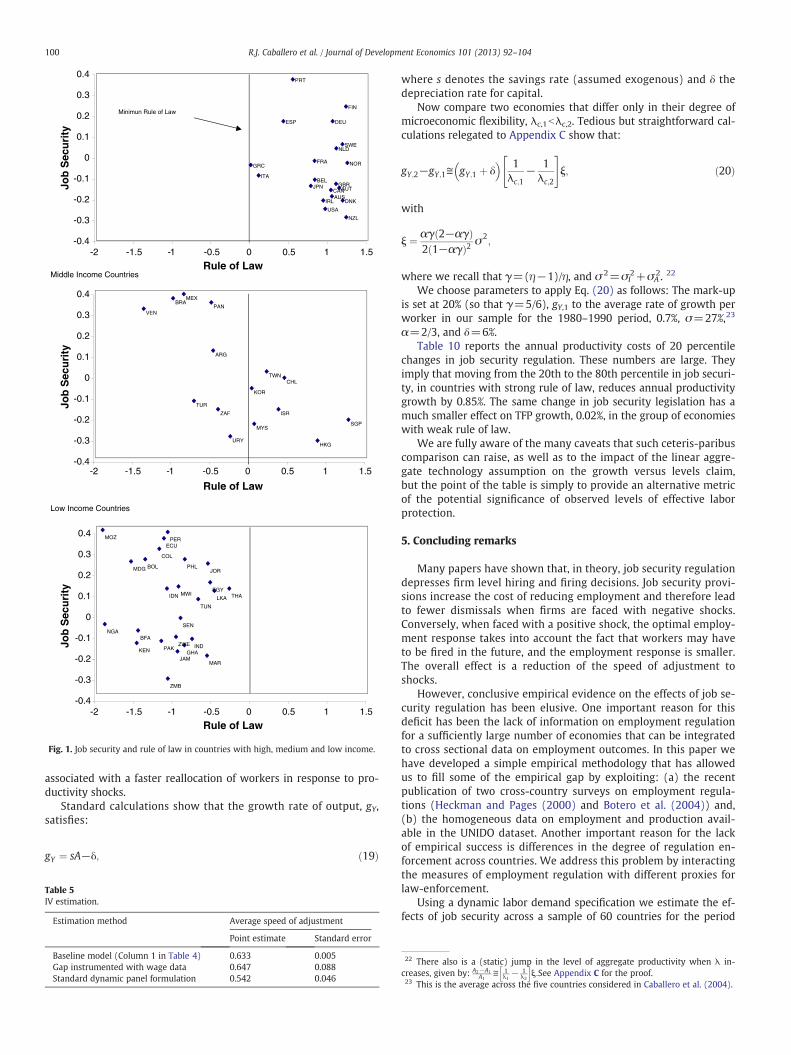
Next, we allow for a distinction between effective and official jobsecurity. Results are reported in columns 3 and 4 (and, correspond-ingly, 6 and 7) for different rules–enforcement criteria. In columns 3and 6 the distinction between effective and official job security is cap-tured by the product of JSc and DSRLc, where DSRLc is a dummy var-iable for countries with strong rule of law (RLc≥RLGreece — whereGreece is the OECD country with the lowest RL score). The threepanels in Fig. 1 show the value of the job security index for countriesin the high, medium and low income groups, respectively. Now λ2 be-comes insignificant, while λ3 has the right sign and is highly signifi-cant. That is, the same change in JSc will have a significantly larger(downward) effect on the speed of adjustment in countries withstricter enforcement of laws, as measured by our rule-of-lawdummy. The effect of the estimated coefficients reported in column3 is large. In countries with strong rule of law, moving from the20th percentile of job security (−0.19) to the 80th percentile (0.23)reduces λ by 0.21. The same change in job security legislation has aconsiderable smaller effect, less than 0.01, on the speed of adjustmentin the group of economies with weak rule of law. That is, employmentadjusts more slowly to shocks in the employment-gap in countrieswith higher levels of effective job security.

Columns 4 and 7 address whether the negative coefficient on λ3 isrobust to other measures of legal enforcement. To do so we use an al-ternative variable from the Kaufmann et al. (1999) dataset – govern-ment effectiveness (GE) – and construct a dummy variable for higheffectiveness countries (GE c≥GEGreece). Clearly, the results are veryclose to those reported in columns 3 and 7. Job security legislationhas a significant negative effect on the estimated speed of adjustmentwhen governments are effective — a proxy for enforcement ofexisting labor regulation.

Finally, the last column in Table 4 uses an alternative measure ofjob security. We repeat our specification from column 7 (includingsector and income dummies) using the Heckman and Pages (2000)measure of job security. The HPct data are only available for countriesin the OECD and Latin America so our sample size is reduced by half,and most low income countries are dropped. The flip side is that thismeasure is time varying which potentially allows us to capture the ef-fects of changes in the job security regulation. As reported in column 8,we find a negative and significant effect of HPct on the speed ofadjustment.

3.3. Further robustness

We continue our robustness exploration by assessing the impact offour broad econometric issues: misspecification due to endogeneity ofthe gap measure, alternative gap-measures, exclusion of potential(country) outliers, and asymmetric adjustment costs.

3.3.1. Potential endogeneity of the gap measureOne concern with our procedure is that the construction of the gap

measure includes the change in employment, that is, the dependentvariable shows up as part of the independent variable. While thisdoes not represent a problem under the null hypothesis of themodel, any measurement error in employment and ϕzjt could intro-duces important biases. We address this issue with two procedures.

The first procedure maintains our baseline specification, but in-struments for the contemporaneous gap measure. Given that Gapjct ¼

Table 3Estimating ϕ.

Specification: (1) (2) (3) (4) (5) (6) (7) (8)

Change in employment (ln)

zjct −0.305 −0.378 −0.558 −0.431 −0.338 −0.395 −0.337 −0.374(0.051)⁎⁎⁎ (0.068)⁎⁎⁎ (0.135)⁎⁎⁎ (0.127)⁎⁎⁎ (0.115)⁎⁎⁎ (0.091)⁎⁎⁎ (0.240) (0.100)⁎⁎⁎

Observations 22,024 21,245 8311 5944 6990 7300 6964 6981Income group All All 1 2 3 All All AllJob sec. group All All All All All 1 2 3Extr. obs. of instrument Yes No No No No No No No

Standard errors are reported in parentheses. All regressions use lagged Δwict−Δw⋅ct as instrumental variable. As described in the main text, zjct represents the log-change of thenominal marginal productivity of labor in each sector, minus the country average, divided by one minus the estimated labor share. All regressions disregard the 2% observationswith most extreme change in employment values and include a country-year fixed effect (κct in Eq. (8)). Income groups are 1: high income OECD, 2: high income non OECD andupper middle income, and 3: lower middle income and low income. Job security groups correspond to the highest, middle and lowest third of the measure in Botero et al. (2004).⁎⁎⁎ Significant at 1%.

98 R.J. Caballero et al. / Journal of Development Economics 101 (2013) 92–104

ϕzjt þ Δejct can be rewritten as ϕzj,t−1+Δejct∗ , a natural instrument isthe lag of the ex-post gap, ϕzjc,t−1. Unfortunately, the latter is not avalid instrument if it is computed with measurement error and thiserror is serially correlated. In our specification this could be the case be-causeweuse amovingaverage to construct the estimateof relative sector-al productivity, θjct . To avoid this problem, we construct an alternativemeasure of the ex-post gap letting wage data play the role of productivitydata when calculating the v and θ terms on the right hand side of (13).

The second procedure re-writes the model in a standard dynamicpanel formulation that removes the contemporaneous employmentchange from the right hand side: 17

ΔGapjct ¼ 1−λcð ÞΔGapjct−1 þ εjct : ð15Þ

Table 5 reports the values of the average λ estimated with thesetwo alternative procedures (note the significant decline in the preci-sion of the estimates). For comparison purposes, the first row repro-duces the first column in Table 4. The second row shows the resultfor the IV procedure based on using lagged changes in wages as in-struments. Finally, row 3 reports the estimate from the dynamicpanel. It is apparent from the table that the estimates of average λare in the right ballpark, and hence we conclude that the bias due toa potentially endogenous gap is not significant.

Finally, we note that the standard solution of passing theΔe-component of the gap defined in Eq. (13) to the left hand side ofthe estimating Eq. (9) does not work in our context. Passing Δe to theleft suggests that the coefficient on the resulting gap will be equal toλ/(1−λ). This holds only in the case of a partial adjustment model.By contrast, when lumpy Calvo-type adjustments are also present, thecorresponding coefficient will, on average, be negative. 18 More impor-tant, even small departures from a partial adjustment model introducesignificant biases when estimating λ using this approach. 19

3.3.2. Alternative gap-measuresTable 4 suggests that conditional on ourmeasure of the employment-

gap, our main findings are robust: job security, when enforced, has asignificant negative impact on the speed of adjustment to theemployment-gap. Table 6 tests the robustness of this result to alter-native measures of the employment-gap. Columns 1 and 2 relax theassumption of a ϕ common across all countries. They repeat our

17 To estimate this equation we follow Anderson and Hsiao (1982) and use twice andthree-times lagged values of ΔGapjct as instruments for the RHS variable. Similar re-sults are obtained if we follow Arellano and Bond (1991).18 In the Calvo-case, for every observation either the (modified) gap or the change inemployment is zero. The former happens when adjustment takes place, the latterwhen it does not. It follows that the covariance of Δe and the (modified) gap will beequal to minus the product of the mean of both variables. Since these means havethe same sign, the estimated coefficient will be negative.19 See Caballero, Engel and Micco (2004) for a formal derivation.

baseline specifications – columns 2 and 3 in Table 4 – using thevalues of ϕ estimated per income-group reported in Table 1. Inturn, columns 3 and 4 report the results of using values of ϕ estimat-ed across countries grouped by level of job security. Countries aregrouped into the upper, middle and lower thirds of job security.Next, columns 5 through 8 repeat our baseline specifications usinga three and four period moving average to estimate θ jct . The finaltwo columns (9 and 10) use an alternative specification for wjct

o basedon average wages instead of average productivity (see Eq. (13)) tobuild Gapjct. In all of the specifications reported in Table 6, our results re-main qualitatively the same as in Table 4.

3.3.3. Exclusion of potential (country) outliersTable 7 reports estimates of λ2 and λ3 using the specification from

column 3 in Table 4 but dropping one country from our sample at atime. In all cases the estimated coefficient on λ3 is negative and signif-icant at conventional confidence intervals.

However, it is also apparent in this table that excluding eitherHong Kong or Kenya makes a substantial difference in the point esti-mates. For this reason, we re-estimate our model from scratch (thatis, from ϕ up) now excluding these two countries. In this case thevalue of ϕ rises from 0.378 to 0.42. Qualitatively, however, the mainresults remain unchanged. Table 8 reports these results.

3.3.4. Asymmetric adjustment costsThere is evidence from establishment level data that hiring is

more costly than firing in some countries (see Pfann and Palm(1993) for the case of the Netherlands and the U.K.). Labor then ad-justs more through the destruction margin than through the creationmargin. This motivates redoing our main results allowing for asym-metric effects of effective job security on the speed of adjustment,depending on whether the hiring or firing margin is operative. Wedo this next and find some evidence for this effect. More importantly,our main result continues holding, namely that the extent to whichlabor regulations hampers adjustment is determined by effective jobsecurity.

Eq. (16) extends Eq. (14) to allow for asymmetric adjustmentspeeds, with Gapn

jct equal to Gapjct þ δct when Gapjct þ δctb0 and zerootherwise and IGapn

jct denoting an indicator function for Gapjct þ δctb0.The parameter λ1n captures the main effect of the differential speedfor negative gaps, and λ2n captures the differential effect of job securityon negative dynamic gaps.

Δejct ¼ λ1Gapjct þ λ1nGapnjct þ λ2 Gapjct � JSc

� �þ λ2n Gapn

jct � JSc� �

þ δct þ γIGapnjct þ εjct : ð16Þ

We run a two-step regression. In the first step we estimate theGapjct+δctb0 which we use in the second step to construct the re-gressors that involve only negative dynamic gaps.

Table 4Estimation results.

(1) (2) (3) (4) (5) (6) (7) (8)

Change in log-employment

Gap (λ1) 0.633 0.636 0.643 0.646(0.005)⁎⁎⁎ (0.007)⁎⁎⁎ (0.008)⁎⁎⁎ (0.008)⁎⁎⁎

Gap×JS (λ2): −0.074 −0.020 −0.029 −0.129 −0.033 −0.044(0.028)⁎⁎⁎ (0.035) (0.035) (0.031)⁎⁎⁎ (0.035) (0.035)

Gap× JS×DSRL (λ3) −0.500 −0.296(0.078)⁎⁎⁎ (0.084)⁎⁎⁎

Gap�JS�DHGE (λ3) −0.502 −0.306(0.078)⁎⁎⁎ (0.085)⁎⁎⁎

Gap×HP (λ2) −0.022(0.008)⁎⁎⁎

ControlsGap×DSRL −0.085 0.089

(0.015)⁎⁎⁎ (0.028)⁎⁎⁎Gap×DHGE −0.099 0.050

(0.016)⁎⁎⁎ (0.028)⁎Observations 21,725 21,725 21,725 21,725 21,725 21,725 21,725 12,011R-squared 0.62 0.62 0.63 0.63 0.63 0.64 0.64 0.64Gap–income interaction No No No No Yes Yes Yes YesGap–sector interaction No No No No Yes Yes Yes Yes

Two-step standard errors in parentheses (Murphy and Topel, 1985). JS and HP stand for the Botero et al. (2004) and Heckman and Pages (2000) job security measures, respectively.DSRL and DHGE stand for strong rule of law and high government efficiency dummies (in both cases the threshold is given by Greece, see the main text), respectively, using theKaufmann et al. (1999) indices. Each regression has country-year fixed effects. Gaps are estimated using a constant ϕ=0.378. Sample excludes the upper and lower 1% of Δeand of the estimated values of Gap.⁎ Significant at 10%.

⁎⁎ Significant at 5%.⁎⁎⁎ Significant at 1%.

99R.J. Caballero et al. / Journal of Development Economics 101 (2013) 92–104

Table 9 reports our results, which may be viewed as an exten-sion of column (2) in Table 6 allowing different responses to posi-tive and negative dynamic employment gaps. From column (1) wesee that the effect of Job Security is present essentially for negativegaps, as (λ2) in column (1) is small and not statistically differentfrom zero while (λ2n) is large and negative, as well as significant.This suggests that Job Security works more through the destructionmargin rather than through the creation margin. Columns (2) and(3), that split the sample between high and low Rule of Law coun-tries, confirm our previous results. Job Security reduces the speedof adjustment in countries with strong rule of law without any no-table differences between the hiring and firing margins: λ2n equalszero for all practical purposes now. As shown in column (3), forcountries with weak rule of law we have a smaller overall employ-ment response to our Job Security measure, also with no significantasymmetries.

4. Gauging the costs of effective labor protection

By impairing worker movements from less to more productiveunits, effective labor protection reduces aggregate output and slowsdown economic growth. In this section we develop a simple frame-work to quantify this effect. Any such exercise requires strong as-sumptions and our approach is no exception. Nonetheless, ourfindings suggest that the costs of the microeconomic inflexibilitycaused by effective protection is large. In countries with strong ruleof law, moving from the 20th to the 80th percentile of job securitylowers annual productivity growth by close to one percentage point.The same movement for countries with weak rule of law has a negli-gible impact on TFP. 20

Consider a continuum of establishments, indexed by i, that adjustlabor in response to productivity shocks, while their share of the

20 Of course, a weak rule of law has an adverse impact on productivity through vari-ous channels not considered in this paper.

economy's capital remains fixed over time. Their production functionsexhibit constant returns to (aggregate) capital, Kt, and decreasingreturns to labor:

Yit ¼ BitKtLαit ; ð17Þ

where Bit denotes plant-level productivity and 0bαb1. The Bit's followgeometric random walks, that can be decomposed into the product ofa common and an idiosyncratic component:

ΔlogBit ≡ bit ¼ vt þ vIit ;

where the vt are i.i.d.N μA;σ2A

� �and the vitI 's are i.i.d. (across productive

units, over time and with respect to the aggregate shocks) N 0;σ2I

� �.

We set μA=0, since we are interested in the interaction between rigid-ities and idiosyncratic shocks, not in Jensen-inequality-type effects as-sociated with aggregate shocks.

The price-elasticity of demand is η>1. Aggregate labor is as-sumed constant and set equal to one. We define aggregate productiv-ity, At, as:

At ¼ ∫BitLαit di; ð18Þ

so that aggregate output, Yt≡∫Yitdi, satisfies

Yt ¼ AtKt :

Units adjust with probability λc in every period, independent oftheir history and of what other units do that period. 21 The parameterthat captures microeconomic flexibility is λc. Higher values of λc are

21 More precisely, whether unit i adjusts at time t is determined by a Bernoulli ran-dom variable ξit with probability of success λc, where the ξit's are independent acrossunits and over time. This corresponds to the case ζ=1 in Section 2.1.

Middle Income Countries

Low Income Countries

AUS

AUT

BEL

CAN

DEU

DNK

ESP

FIN

FRA

GBR

GRC

IRL

ITA

JPN

NLD

NOR

NZL

PRT

SWE

USA

-0.4

-0.3

-0.2

-0.1

0

0.1

0.2

0.3

0.4

-2 -1.5 -1 -0.5 0 0.5 1 1.5

Rule of Law

Job

Sec

uri

ty

ZAF

VEN

URY

TWN

TUR

SGP

PAN

MYS

MEX

KOR

ISR

HKG

CHL

BRA

ARG

-0.4

-0.3

-0.2

-0.1

0

0.1

0.2

0.3

0.4

-2 -1.5 -1 -0.5 0 0.5 1 1.5

Rule of Law

Job

Sec

uri

ty

ZWE

ZMB

TUN

THA

SEN

PHL

PER

PAK

NGA

MWI

MOZ

MDG

MAR

LKA

KEN

JOR

JAM

IND

IDN

GHA

EGY

ECU

COL

BOL

BFA

-0.4

-0.3

-0.2

-0.1

0

0.1

0.2

0.3

0.4

-2 -1.5 -1 -0.5 0 0.5 1 1.5

Rule of Law

Job

Sec

uri

ty

Minimun Rule of Law

Fig. 1. Job security and rule of law in countries with high, medium and low income.

100 R.J. Caballero et al. / Journal of Development Economics 101 (2013) 92–104

associated with a faster reallocation of workers in response to pro-ductivity shocks.

Standard calculations show that the growth rate of output, gY,satisfies:

gY ¼ sA−δ; ð19Þ

Table 5IV estimation.

Estimation method Average speed of adjustment

Point estimate Standard error

Baseline model (Column 1 in Table 4) 0.633 0.005Gap instrumented with wage data 0.647 0.088Standard dynamic panel formulation 0.542 0.046

where s denotes the savings rate (assumed exogenous) and δ thedepreciation rate for capital.

Now compare two economies that differ only in their degree ofmicroeconomic flexibility, λc,1bλc,2. Tedious but straightforward cal-culations relegated to Appendix C show that:

gY;2−gY;1≅ gY;1 þ δ� � 1

λc;1− 1

λc;2

" #ξ; ð20Þ

with

ξ ¼ αγ 2−αγð Þ2 1−αγð Þ2 σ2

;

where we recall that γ=(η−1)/η, and σ 2=σI2+σA

2. 22

We choose parameters to apply Eq. (20) as follows: The mark-upis set at 20% (so that γ=5/6), gY,1 to the average rate of growth perworker in our sample for the 1980–1990 period, 0.7%, σ=27%,23

α=2/3, and δ=6%.Table 10 reports the annual productivity costs of 20 percentile

changes in job security regulation. These numbers are large. Theyimply that moving from the 20th to the 80th percentile in job securi-ty, in countries with strong rule of law, reduces annual productivitygrowth by 0.85%. The same change in job security legislation has amuch smaller effect on TFP growth, 0.02%, in the group of economieswith weak rule of law.

We are fully aware of the many caveats that such ceteris-paribuscomparison can raise, as well as to the impact of the linear aggre-gate technology assumption on the growth versus levels claim,but the point of the table is simply to provide an alternative metricof the potential significance of observed levels of effective laborprotection.

5. Concluding remarks

Many papers have shown that, in theory, job security regulationdepresses firm level hiring and firing decisions. Job security provi-sions increase the cost of reducing employment and therefore leadto fewer dismissals when firms are faced with negative shocks.Conversely, when faced with a positive shock, the optimal employ-ment response takes into account the fact that workers may haveto be fired in the future, and the employment response is smaller.The overall effect is a reduction of the speed of adjustment toshocks.

However, conclusive empirical evidence on the effects of job se-curity regulation has been elusive. One important reason for thisdeficit has been the lack of information on employment regulationfor a sufficiently large number of economies that can be integratedto cross sectional data on employment outcomes. In this paper wehave developed a simple empirical methodology that has allowedus to fill some of the empirical gap by exploiting: (a) the recentpublication of two cross-country surveys on employment regula-tions (Heckman and Pages (2000) and Botero et al. (2004)) and,(b) the homogeneous data on employment and production avail-able in the UNIDO dataset. Another important reason for the lackof empirical success is differences in the degree of regulation en-forcement across countries. We address this problem by interactingthe measures of employment regulation with different proxies forlaw-enforcement.

Using a dynamic labor demand specification we estimate the ef-fects of job security across a sample of 60 countries for the period

22 There also is a (static) jump in the level of aggregate productivity when λ in-creases, given by: A2−A1

A1≅ 1

λ1− 1

λ2

h iξ:See Appendix C for the proof.

23 This is the average across the five countries considered in Caballero et al. (2004).

Table 6Robustness of main results to alternative specifications.

ϕ varies across ϕ varies across ϕ=0.378

Income groups Job security groups θ=MA(3) θ=MA(4) dw

(1) (2) (3) (4) (5) (6) (7) (8) (9) (10)

Change in log-employment

Gap 0.636 0.643 0.594 0.560 0.638(0.007)⁎⁎⁎ (0.005)⁎⁎⁎ (0.007)⁎⁎⁎ (0.007)⁎⁎⁎ (0.007)⁎⁎⁎

Gap×JS −0.074 −0.033 −0.041 −0.001 −0.047 0.005 −0.016 0.052 −0.076 −0.028(0.028)⁎⁎⁎ (0.035) (0.028) (0.035) (0.028)⁎ (0.035) (0.028) (0.035) (0.030)⁎⁎ (0.037)

Gap×DSRL 0.089 0.104 0.079 0.065 0.076(0.028)⁎⁎⁎ (0.027)⁎⁎⁎ (0.027)⁎⁎⁎ (0.026)⁎⁎ (0.028)⁎⁎⁎

Gap�JS�DSRL −0.296 −0.236 −0.306 −0.364 −0.327(0.084)⁎⁎⁎ (0.084)⁎⁎⁎ (0.081)⁎⁎⁎ (0.080)⁎⁎⁎ (0.088)⁎⁎⁎

Observations 21,725 21,725 20,897 20,215 21,295R-squared 0.62 0.64 0.63 0.64 0.61 0.63 0.60 0.61 0.62 0.63Gap–sector int. No Yes No Yes No Yes No Yes No Yes

Two-step standard errors in parentheses (Murphy and Topel, 1985). JS stands for the Botero et al. (2004) job security measure. DSRL stands for high (above Greece, see main text)rule of law using the Kaufmann et al. (1999) measure. Columns (1), (2), (3) and (4) use values of ϕ estimated in Table 3. Samples exclude the upper and lower 1% of Δe and of theestimated values of Gap.

⁎ Significant at 10%.⁎⁎ Significant at 5%.

⁎⁎⁎ Significant at 1%.

101R.J. Caballero et al. / Journal of Development Economics 101 (2013) 92–104

from 1980 to 1998. We consistently find a relatively lower speed ofadjustment of employment in countries with high legal protectionagainst dismissal, especially when such protection is likely to beenforced.

Appendix A. Representative firm's frictionless problem

Proposition 1. A firm with production function Y=AEαHβ faces (in-verse) demand P=DY−1/η, where Y, E, H, P, A and D denote output, em-ployment, hours per worker, price, productivity shock and demandshock, respectively. We denote γ≡(η−1)/η and assume η>1,α>β>0 and αγb1. The firm faces a wage schedule W(H), and we de-fine w(h)≡ logW(eh). We assume w′>0, w″>0, w′(0)bβ/αbw′(+∞)and W″ H

� �> 0, with H defined via Eq. (21) below. In general, lower

case letters denote the logs of upper case variables.Then the values of h and e that solve the firm's static optimization

problem are denoted by h and e and characterized by:

w′ h� �

¼ βα; ð21Þ

e ¼ 11−αγ

log βγ þ dþ γa− 1−βγð Þh−log W ′ H� �n oh i

: ð22Þ

Proof. The firm's (static) profit function is

Π E;Hð Þ≡DAγEαγHβγ−W Hð ÞE:

The corresponding partial derivatives and first order conditionsthen are:

∂Π∂E ¼ αγDAγEαγ−1Hβγ−W Hð Þ ¼ 0; ð23Þ

∂Π∂H ¼ βγDAγEαγHβγ−1−W ′ Hð ÞE ¼ 0: ð24Þ

Multiplying Eq. (23) by (βE)/(αH), subtracting Eq. (24), and notingthat w′(h)=W′(H)H/W(H) leads to the first order condition w′(h)=

β/α. This equation has a unique solution due to the assumptions wemade for w. Expression (22) follows from taking logs in Eq. (24).

Next we check that the second order conditions hold at h and e.From Eqs. (23) to (24) we have

∂2Π∂E2

¼ −αγ 1−αγð ÞDAγEαγ−2Hβγ; ð25Þ

∂2Π∂H2 ¼ −βγ 1−βγð ÞDAγEαγHβγ−2−W″ Hð Þ; ð26Þ

∂2Π∂E∂H ¼ αβγ2DAγEαγ−1Hβγ−1−W ′ Hð Þ

¼ −βγ 1−αγð ÞDAγEαγ−1Hβγ−1; ð27Þ

where in the last step we used Eq. (24) evaluated at H .We therefore have ∂ 2Π/∂E2b0, while Eqs. (25), (26) and (27) can

be used to show that

∂2Π∂E2

∂2Π∂H2 − ∂2Π

∂E∂H

" #2¼ βγ2 1−αγð Þ α−βð ÞD2A2γE2αγ−2H2βγ−2

þ αγ 1−αγð ÞDAγEαγ−1HβγW″ Hð Þ:

The first term on the r.h.s. is positive because we assumed α>β andαγb1. The second term is positive because we assumed W″ H

� �> 0.

Appendix B. Relation between static and dynamic targets

Proposition 2. The firm's static employment target, et , satisfies:

et ¼ et−1 þ gt þ εt ;

with εt i.i.d. innovations with zero mean and variance σe2. The drift, gt, is

observed by the firm and satisfies:

gt−g ¼ ρ gt−1−gð Þ þ νt ;

with 0≤ρ≤1 and νt i.i.d. innovations with zero mean and variance σν2,

independent from the εts.

24 That is, we ignore hours in the production function.

Table 7Excluding one country at a time.

Country λ2 λ3 Country λ2 λ3

Coeff. St.dev.

Coeff. St.dev.

Coeff. St.dev.

Coeff. St.dev.

ARG −0.01 0.05 −0.51 0.07 KOR −0.02 0.05 −0.52 0.07AUS −0.02 0.05 −0.52 0.07 LKA −0.02 0.05 −0.51 0.07AUT −0.02 0.05 −0.52 0.07 MAR −0.02 0.05 −0.51 0.07BEL −0.02 0.05 −0.52 0.07 MDG −0.02 0.05 −0.51 0.07BFA −0.03 0.05 −0.50 0.07 MEX 0.00 0.05 −0.53 0.07BOL 0.00 0.05 −0.52 0.07 MOZ 0.02 0.05 −0.55 0.07BRA −0.01 0.05 −0.52 0.07 MWI −0.01 0.05 −0.52 0.07CAN −0.02 0.05 −0.52 0.07 NYS −0.02 0.05 −0.46 0.07CHL −0.02 0.05 −0.53 0.07 NGA 0.00 0.05 −0.53 0.07COL −0.02 0.05 −0.51 0.07 NLD −0.02 0.05 −0.51 0.07DEU −0.02 0.05 −0.52 0.07 NOR −0.02 0.05 −0.51 0.07DNK −0.02 0.05 −0.52 0.07 NZL −0.02 0.05 −0.53 0.07ECU −0.03 0.05 −0.50 0.07 PAK 0.02 0.05 −0.55 0.07EGY −0.02 0.05 −0.51 0.07 PAN −0.01 0.05 −0.52 0.07ESP −0.02 0.05 −0.53 0.07 PER 0.06 0.05 −0.59 0.07FIN −0.02 0.05 −0.54 0.07 PHL −0.03 0.05 −0.50 0.07FRA −0.02 0.05 −0.51 0.07 PRT −0.02 0.05 −0.54 0.07GBR −0.02 0.05 −0.51 0.07 SEN 0.00 0.05 −0.53 0.07GHA −0.05 0.05 −0.48 0.07 SGP −0.02 0.05 −0.52 0.07GRC −0.02 0.05 −0.51 0.07 SWE −0.02 0.05 −0.53 0.07HKG −0.02 0.05 −0.37 0.07 THA −0.01 0.05 −0.51 0.07IDN −0.02 0.05 −0.51 0.07 TUN −0.02 0.05 −0.51 0.07IND 0.01 0.05 −0.54 0.07 TUR −0.03 0.05 −0.50 0.07IRL −0.02 0.05 −0.54 0.07 TWN −0.02 0.05 −0.49 0.07ISR −0.02 0.05 −0.52 0.07 URY −0.02 0.05 −0.50 0.07ITA −0.02 0.05 −0.51 0.07 USA −0.02 0.05 −0.53 0.07JAM −0.02 0.05 −0.51 0.07 VEN 0.00 0.05 −0.53 0.07JOR −0.04 0.05 −0.49 0.07 ZAF −0.02 0.05 −0.51 0.07JPN −0.02 0.05 −0.52 0.07 ZMB −0.02 0.05 −0.51 0.07KEN −0.15 0.05 −0.38 0.07 ZWE 0.03 0.05 −0.55 0.07

This table reports the estimated coefficients for λ2 and λ3, for the specification incolumn 3 of Table 4, leaving out one country (the one indicated for each set ofcoefficients) at a time.

102 R.J. Caballero et al. / Journal of Development Economics 101 (2013) 92–104

The firm's discount factor is β and its adjustment technology is Calvo,that is, in every period it either adjusts at no cost (with probability λ) orit cannot adjust (with probability 1−λ). The firm's loss from deviatingfrom its static target is quadratic in the employment log-difference,

Then the firm's dynamic employment target, that is, its optimal em-ployment choice should it adjust, is given by:

e�t ¼ et þ δt ð28Þ

with

δt≡β 1−λð Þ

1−β 1−λð Þ g þ β 1−λð Þρ1−β 1−λð Þρ gt−gð Þ: ð29Þ

Proof. If the firm adjusts in t, it will choose its employment level, et∗,so as to minimize the expected cost of deviating from its static targetduring the period where the new price is in place:

Et∑k≥0

β 1−λð Þ½ �k e�t−etþk

� �2:

It follows that:

e�t ¼ 1−β 1−λð Þ½ �∑k≥0

β 1−λð Þ½ �kEt etþk: ð30Þ

The assumptions for et imply that

etþk ¼ et þXki¼1

gtþi þXki¼1

εtþi;

and therefore

Et etþk ¼ et þ kg þ ρ1−ρ

1−ρk� �

gt−gð Þ:

Substituting this expression in Eq. (30) yields Eqs. (28) and (29).

Appendix C. Gauging the costs

In this appendix we derive Eq. (20). From Eqs. (19) to (20) it fol-lows that it suffices to show that under the assumptions in Section 4we have:

A2−A1

A1≅ 1

λ1− 1

λ2

� �ξ; ð31Þ

where we have dropped the subindex c from the λ and

ξ ¼ αγ 2−αγð Þ2 1−αγð Þ2 σ2

I þ σ2A

� �: ð32Þ

The intuition is easier if we consider the following, equivalent,problem. The economy consists of a very large and fixed number offirms (no entry or exit). Production by firm i during period t is Yi,t=Ai,tLi,t

α , 24 while (inverse) demand for good i in period t is Pi,t=Yi,t−1/η,

where Ai,t denotes productivity shocks, assumed to follow a geometricrandom walk, so that

ΔlogAi;t≡Δai;t ¼ vAt þ vIi;t ;

with vtA i.i.d. N(0,σA

2) and vi,tI i.i.d. N(0,σI

2). Hence Δai,t follows aN(0,σT

2), with σT2=σA

2+σI2. We assume the wage remains constant

throughout.In what follows lower case letters denote the logarithm of upper

case variables. Similarly, ∗-variables denote the frictionless counter-part of the non-starred variable.

Solving the firm's maximization problem in the absence of adjust-ment costs leads to:

Δl�i;t ¼γ

1−αγΔai;t ; ð33Þ

and hence

Δy�i;t ¼1

1−αγΔai;t : ð34Þ

Denote by Yt∗ aggregate production in period t if there were no fric-

tions. It then follows from Eq. (24) that:

Y�i;t ¼ eτΔai;t Y�

i;t−1; ð35Þ

with τ≡1/(1−αγ), Taking expectations (over i for a particular reali-zation of vtA) on both sides of Eq. (35) and noting that both termsbeing multiplied on the r.h.s. are, by assumption, independent (ran-dom walk), yields

Y�t ¼ eτv

At þ1

2τ2σ2

I Y�t−1; ð36Þ

Averaging over all possible realizations of vtA (these fluctuationsare not the ones we are interested in for the calculation at hand)leads to

Y�t ¼ e

12τ

2σ2T Y�

t−1;

Table 8Estimation results excluding Hong Kong and Kenya.

(1) (2) (3) (4) (5) (6) (7) (8)

Change in log-employment

Gap (λ1) 0.641 0.645 0.674 0.676(0.007)⁎⁎⁎ (0.007)⁎⁎⁎ (0.008)⁎⁎⁎ (0.008)⁎⁎⁎

Gap×JS (λ2): −0.094 −0.145 −0.151 −0.197 −0.163 −0.175(0.031)⁎⁎⁎ (0.037)⁎⁎⁎ (0.037)⁎⁎⁎ (0.032)⁎⁎⁎ (0.037)⁎⁎⁎ (0.037)⁎⁎⁎

Gap�JS�DSRL (λ3) −0.230 −0.064(0.085)⁎⁎⁎ (0.089)

Gap�JS�DHGE (λ3) −0.227 −0.073(0.085)⁎⁎⁎ (0.089)

Gap×HP (λ2) −0.021(0.008)⁎⁎

ControlsGap×DSRL −0.122 −0.070

(0.016)⁎⁎⁎ (0.028)⁎⁎Gap×DHGE −0.136 0.028

(0.016)⁎⁎⁎ (0.028)Observations 20,903 20,903 20,903 20,903 20,903 20,903 20,903 12,004R-squared 0.63 0.63 0.63 0.63 0.64 0.64 0.64 0.64Gap–income interaction No No No No Yes Yes Yes YesGap–sector interaction No No No No Yes Yes Yes Yes

Two-step standard errors in parentheses (Murphy and Topel, 1985). JS and HP stand for the Botero et al. (2004) and Heckman and Pages (2000) job security measures, respectively.DSRL and DHGE stand for high (above Greece, see main text) rule of law and government efficiency dummies, respectively, using the Kaufmann et al. (1999) indices. Each regres-sion has country-year fixed effects. Gaps are estimated using a constant ϕ=0.42. Sample excludes the upper and lower 1% of Δe and of the estimated values of gap.⁎ Significant at 10%.

⁎⁎ Significant at 5%.⁎⁎⁎ Significant at 1%.

103R.J. Caballero et al. / Journal of Development Economics 101 (2013) 92–104

and therefore for k=1,2,3,…:

Y�t ¼ e

12kτ

2σ2T Y�

t−k: ð37Þ

Denote:

• Yt,t−k: aggregate Y that would attain in period t if firms had the fric-tionless optimal levels of labor corresponding to period t-k. This isthe average Y for units that last adjusted k periods ago.

• Yi,t,t−k: the corresponding level of production of firm i in t.

Table 9Asymmetric responses.

(1) (2) (3)

Change in log-employment

Gap (λ1): 0.688 0.583 0.697(0.011)⁎⁎⁎ (0.027)⁎⁎⁎ (0.016)⁎⁎⁎

Gapn (λ1n): −0.032 0.001 −0.026(0.018)⁎ (0.035) (0.025)

Gap×JS (λ2): 0.006 −0.491 0.070(0.050) (0.129)⁎⁎⁎ (0.070)

Gapn×JS (λ2n): −0.189 −0.002 −0.191(0.008)⁎⁎ (0.189) (0.115)⁎

IGapn 0.015 0.006 0.021(0.001)⁎⁎⁎ (0.002)⁎⁎⁎ (0.004)⁎⁎⁎

Observations 21,725 11,848 9877R-squared 0.63 0.67 0.61Rule of law All High Low

JS stand sfor the Botero et al. (2004) job security measure. rule of law (the threshold isgiven by Greece, see the main text) from Kaufmann et al. (1999) indices. Eachregression has country-year fixed effects. Gaps are estimated using a constant ϕ=0.378. Sample excludes the upper and lower 1% of Δe and of the estimated values ofgap.

⁎ Significant at 10%.⁎⁎ Significant at 5%.

⁎⁎⁎ Significant at 1%.

From the expressions derived above it follows that:

Yi;t;t−1

Y�i;t

¼ L�i;t−1

L�i;t

!α

¼ e−αγτΔai;t ;

and therefore

Yi;t;t−1 ¼ eΔai;t Y�i;t−1:

Taking expectations (with respect to idiosyncratic and aggregateshocks) on both sides of the latter expression (here we use that Δai,tis independent of Yi,t−1

∗ ) yields

Yt;t−1 ¼ e12σ

2T Y�

t−1;

which combined with Eq. (37) leads to:

Yt;t−1 ¼ e12 1−τ2ð Þσ2

T Y�t :

A derivation similar to the one above, leads to:

Yi;t;t−k ¼ eΔai;tþΔai;t−1þ…þΔai;t−kþ1Y�t−k;

Table 10Productivity growth and job security.

Change in job security index Cost in annual growth rate

Weak rule of law Strong rule of law

20th to 40th percentile 0.002% 0.083%40th to 60th percentile 0.007% 0.292%60th to 80th percentile 0.008% 0.478%

Reported: change in annual productivity growth rates associated with moving acrosspercentiles in the distribution of country job security measures computed in Boteroet al. (2004). Lower values of job security index correspond to less job security.Values of speed of adjustment calculated using Column 3 in Table (4). The thresholdfor weak and strong rule of law is given by the OECD country with the lowest rule oflaw score (Greece). Changes in annual productivity growth calculated based on Eq. (20).Parameter values used: γ=5/6, gY,1=0.007, σ=0.27 α=2/3, and δ=0.06.

104 R.J. Caballero et al. / Journal of Development Economics 101 (2013) 92–104

which combined with Eq. (37) gives:

Yt;t−k ¼ e−kξY�t ; ð38Þ

with ξ defined in Eq. (32).Assuming Calvo-type adjustment with probability λ, we de-

compose aggregate production into the sum of the contributionsof cohorts:

Yt ¼ λY�t þ λ 1−λð ÞYt;t−1 þ λ 1−λð Þ2Yt;t−2 þ…

Substituting Eq. (38) in the expression above yields:

Yt ¼λ

1− 1−λð Þe−ξY�t : ð39Þ

It follows that the production gap, defined as:

Prod: Gap≡Y�t−Yt

Y�t

;

is equal to:

Prod: Gap ¼1−λð Þ 1−e−ξ

� �1− 1−λð Þe−ξ

: ð40Þ

A first-order Taylor expansion then shows that, when |ξ|bb1:

Prod: Gap≅ 1−λð Þλ

ξ: ð41Þ

Subtracting this gap evaluated at λ1 from its value evaluated at λ2,and noting that this gap difference corresponds to (A2−A1)/A1 in themain text, yields Eq. (31) and therefore concludes the proof.

References

Abraham, K., Houseman, S., 1994. Does employment protection inhibit labor marketflexibility: lessons from Germany, France and Belgium. In: Blank, R.M. (Ed.), Pro-tection Versus Economic Flexibility: Is There A Tradeoff? University of ChicagoPress, Chicago.

Addison, J.T., Texeira, P., Grosso, J.L., 2000. The effect of dismissals protection onemployment: more on a vexed theme. Southern Economic Journal 67, 105–122.

Anderson, T.W., Hsiao, C., 1982. Formulation and estimation of dynamic models usingpanel data. Journal of Econometrics 18, 67–82.

Arellano, M., Bond, S.R., 1991. Some specification tests for panel data: Monte Carlo ev-idence and an application to employment equations. Review of Economic Studies58, 277–298.

Botero, J., Djankov, S., La Porta, R., Lopez-de-Silanes, F., Shleifer, A., 2004. The regulationof labor. Quarterly Journal of Economics 119 (4), 1339–1382.

Burgess, S., Knetter, M., 1998. An international comparison of employment adjustmentto exchange rate fluctuations. Review of International Economics 6 (1), 151–163.

Burgess, S., Knetter, M., Michelacci, C., 2000. Employment and output adjustment in theOECD: a disaggregated analysis of the role of job security provisions. Economica 67,419–435.

Caballero, R., Engel, E., 1993. Microeconomic adjustment hazards and aggregate dy-namics. Quarterly Journal of Economics 108 (2), 359–383.

Caballero, R., Hammour, M., 2000. Creative destruction and development: institutions,crises, and restructuring. Annual World Bank Conference on Development Eco-nomics 2000, pp. 213–241.

Caballero, R., Engel, E., Haltiwanger, J., 1997. Aggregate employment dynamics: build-ing from microeconomic evidence. American Economic Review 87 (1), 115–137.

Caballero, R., Engel, E., Micco, A., 2004. Effective labor regulation and microeconomicflexibility. NBER Working Paper No. 10744.

Calvo, G., 1983. Staggered prices in a utility maximizing framework. Journal of Mone-tary Economics 12, 383–398.

Foster, L., Haltiwanger, J., Krizan, C.J., 1998. Aggregate productivity growth: lessonsfrom microeconomic evidence. NBER Working Papers No. 6803.

Freeman, 2001. Institutional Differences and economic performance among OECDcountries. CEP Discussion Papers 0557.

Garibaldi, P., Mauro, P., 1999. Deconstructing job creation. International MonetaryFund Working Paper WP/99/109.

Grubb, D., Well, W., 1993. Employment regulation and patterns of work in the EC coun-tries. OECD Economic Studies No. 21, Winter.

Hamermesh, D., 1993. Labor Demand. Princeton University Press, Princeton.Heckman, J., Pages, C., 2000. The cost of job security regulation: evidence from Latin

American labor markets. Inter-American Development Bank Working Paper 430.Heckman, J., Pagés, C., 2003. Law and employment: lessons from Latin America and the

Caribbean. NBER Working Paper No. 10129.Kaufmann, D., Kraay, A., Zoido-Lobaton, P., 1999. Governance matters. World Bank Pol-

icy Research Department Working Paper No. 2196.Lazear, E., 1990. Job security provisions and employment. Quarterly Journal of Econom-

ics 105 (3), 699–726.Loboguerrero, A.M., Panizza, U., 2003. Inflation and labor market flexibility: the

squeakly wheal gets the grease. Working Paper 495. Research Department, Inter-American Development Bank.

Murphy, K.M., Topel, R.H., 1985. Estimation and inference in two-step econometricmodels. Journal of Business and Economic Statistics 3 (4), 370–379.

Nickell, S., 1986. Dynamic models of labour demand. In: Ashenfelter, O., Layard, R.(Eds.), Handbook of Labor Economics. Elsevier.

Nickell, S., 1997. Unemployment and labor market rigidities: Europe versus NorthAmerica. Journal of Economic Perspectives 11 (3), 55–74.

Nickell, S., Nunziata, L., 2000. Employment patterns in OECD countries. Center for Eco-nomic Performance Discussion Paper No. 448.

OECD, 1999. Employment protection and labor market performance. OECD EconomicOutlook. OECD, Paris . (Chapter 2).

Pfann, G., Palm, F.C., 1993. Asymmetric adjustment costs in non-linear labour demandmodels for the Netherlands and U.K. manufacturing sectors. Review of EconomicStudies 60 (2), 397–412.

Sargent, T., 1978. Estimation of dynamic labor demand under rational expectations.Journal of Political Economy 86, 1009–1044.

Shapiro, M.D., 1986. The Dynamic demand for capital and labor. Quarterly Journal ofEconomics 101, 513–542.

UNIDO, 2002. Industrial Statistics Database 2002 (3-digit level of ISIC code (Revision 2)).