Effective Dynamics of Bianchi-I spacetime in

LQC: Kasner transitions and inflationary scenario

Brajesh Gupt(based on arXiv:1205.6763v2 and work to appear with Parampreet Singh)

Louisiana State University

International Loop Quantum Gravity Seminar

March 26 , 2013

Why study Bianchi models?

Anisotropic spacetime introduces more degrees of freedomcompared to isotropic spacetime

Much richer physics due to non-vanishing Weyl scalar

Classically the anisotropic shear scalar in Bianchi-I model variesas σ2 ∝ a−6. Singularity can also take place due to diverginganisotropic shear as a→ 0

According to Belinskii-Khalatnikov-Lifshitz (BKL) behavior,during a generic approach to a spacelike singularity, each pointtransits from one Bianchi-I type universe to another Bianchi-Itype (Kasner transition), giving rise to Mixmaster behavior

2

Loop quantum cosmology of Bianchi-I spacetime

ds2 = −dt2 + a21 dx2 + a22 dy

2 + a23 dz2

In the classical theory, approach to singularity can be classified as(Doroshkevich, Ellis, Jacobs, MacCallum, Thorne ...)

Point or Isotropic singularity: a1, a2, a3 → 0.Barrel: a1 → const, a2, a3 → 0Pancake: a1 → 0, a2, a3 → constCigar: a1 →∞, a2, a3 → 0

Quantization performed by (Ashtekar, Wilson-Ewing(09)). Earlierapproaches to quantization developed by Bojowald, Chiou, Date,

Martin-Benito, Mena Marugan, Pawlowski, Szulc, Vandersloot

Classical singularity resolvedResolution of all physical singularities studied in the effectivedynamics (Singh (11))Physics of effective dynamics studied: big bang is replaced bybounce (Artymowski, Cailleteau, Chiou, Lalak, Maartens, Singh,

Vandersloot)3

Questions:

Kasner Transitions:

What is the relation between the geometrical nature ofspacetime in pre and post bounce regime?

Are there transitions from one type to other?

Are some transitions favored over others? If yes, depending onwhat?

Inflation:

Does anisotropy prevent inflation?

How does LQC modify the dynamics and the amount ofinflation?

How is the amount of inflation affected as compared to theisotropic spacetime?

4

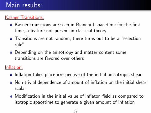
Main results:

Kasner Transitions:

Kasner transitions are seen in Bianchi-I spacetime for the firsttime, a feature not present in classical theory

Transitions are not random, there turns out to be a “selectionrule”

Depending on the anisotropy and matter content sometransitions are favored over others

Inflation:

Inflation takes place irrespective of the initial anisotropic shear

Non-trivial dependence of amount of inflation on the initial shearscalar

Modification in the initial value of inflaton field as compared toisotropic spacetime to generate a given amount of inflation

5

Plan of the talk:

Review of Kasner solution

Review of effective dynamics of Bianchi-I

Kasner transitions with perfect fluid with P = ρ

Inflation in Bianchi-I spacetime with quadratic potentialV (φ) = m2φ2/2

6

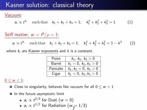
Kasner solution: classical theory

Vacuum:

ai ∝ tki such that k1 + k2 + k3 = 1; k21 + k2

2 + k23 = 1 (1)

Stiff matter, w = P/ρ = 1:

ai ∝ tki such that k1 + k2 + k3 = 1; k21 + k2

2 + k23 = 1− k2 (2)

where ki are Kasner exponents and k is a constant.

Point k1, k2, k3 > 0Barrel k1 = 0, k2, k3 > 0

Pancake k1, k2 = 0, k3 > 0Cigar k1 < 0, k2, k3 > 0

0 ≤ w < 1:

Close to singularity, behaves like vacuum for all 0 ≤ w < 1

In the future asymptotic limit

ai ∝ t2/3 for Dust (w = 0)ai ∝ t1/2 for Radiation (w = 1/3)

7

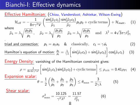
Bianchi-I: Effective dynamics

Effective Hamiltonian: (Chiou, Vandersloot; Ashtekar, Wilson-Ewing)

Heff = − 1

8πγ2V

(sin(µ1c1)

µ1

sin(µ2c2)

µ2p1p2 + cyclic terms

)+Hmatt , (1)

whereµ1 = λ

√p2p3p1

, µ2 = λ

√p1p3p2

µ3 = λ

√p2p1p3

and λ2 = 4√

3πγ`2Pl

.triad and connection: p1 = a2a3 & classically, c1 = γa1 (2)

Hamilton’s equation of motion: p1p1

= 1γλ

[sin(µ2c2) + sin(µ3c3)

]cos(µ1c1) (3)

Energy Density: vanishing of the Hamiltonian constraint gives:

ρ = 18πGγ2λ2

[sin(µ1c1) sin(µ2c2) + cyclic terms

]≤ ρcrit = 0.41ρPl (4)

Expansion scalar:θ =

1

2

(p1p1

+p2p2

+p3p3

)≤ θmax =

3

2γλ(5)

Shear scalar:σ2

max =10.125

γ2λ2=

11.57

`2Pl

(6)

8

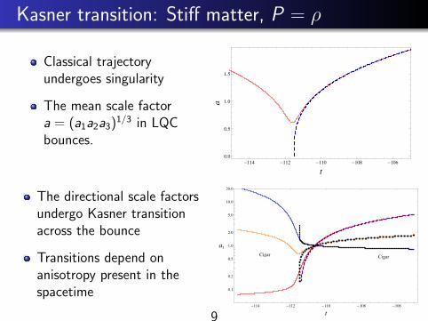
Kasner transition: Stiff matter, P = ρ

Classical trajectoryundergoes singularity

The mean scale factora = (a1a2a3)1/3 in LQCbounces.

-114 -112 -110 -108 -106

0.0

0.5

1.0

1.5

t

a

The directional scale factorsundergo Kasner transitionacross the bounce

Transitions depend onanisotropy present in thespacetime

Cigar Cigar

-114 -112 -110 -108 -106

0.1

0.2

0.5

1.0

2.0

5.0

10.0

20.0

t

ai

9

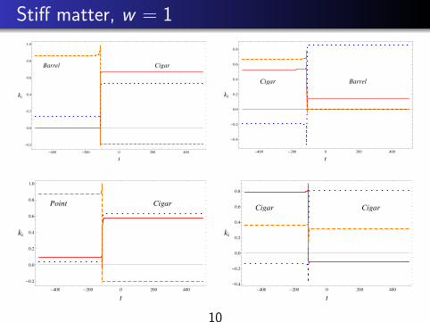
Stiff matter, w = 1

CigarBarrel

-400 -200 0 200 400

-0.2

0.0

0.2

0.4

0.6

0.8

1.0

t

ki

BarrelCigar

-400 -200 0 200 400

-0.4

-0.2

0.0

0.2

0.4

0.6

0.8

t

ki

CigarPoint

-400 -200 0 200 400

-0.2

0.0

0.2

0.4

0.6

0.8

1.0

t

ki

CigarCigar

-400 -200 0 200 400

-0.4

-0.2

0.0

0.2

0.4

0.6

0.8

t

ki

10

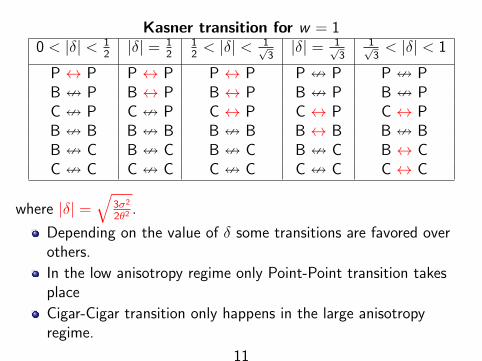
Kasner transition for w = 10 < |δ| < 1

2|δ| = 1

212< |δ| < 1√

3|δ| = 1√

31√3< |δ| < 1

P ↔ P P ↔ P P ↔ P P = P P = PB = P B ↔ P B ↔ P B = P B = PC = P C = P C ↔ P C ↔ P C ↔ PB = B B = B B = B B ↔ B B = BB = C B = C B = C B = C B ↔ CC = C C = C C = C C = C C ↔ C

where |δ| =√

3σ2

2θ2.

Depending on the value of δ some transitions are favored overothers.

In the low anisotropy regime only Point-Point transition takesplace

Cigar-Cigar transition only happens in the large anisotropyregime.

11

Inflation

Inflation: a phase of accelerated expansion in the early universeWidely studied and explored in the classical theory. (Albrecht, Barrow,

Guth, Linde, Rothman, Steinhardt, Steigman, Turner...)

Does anisotropy prevent inflation? Barrow and Turner (81); Steigman

and Turner (83)

Quantum theory of gravity is required (Rothman & Madsen (85),

Rothman & Ellis(86)); Anisotropy helps attain more inflation(Maartens, Sahni and Saini (01))

Inflation in LQC in isotropic spacetime...(Ashtekar, Pawlowski, Singh

to appear)

Isotropic inflation in effective theory studied in detail by Ashtekar

& Sloan (09) establishing its inevitability (99.99%); other aspectsalso studied by Corichi & Karami (10)

12

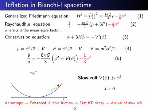
Inflation in Bianchi-I spacetime

Generalized Friedmann equation: H2 =(aa

)2= 8πG

3ρ+1

6σ2 (1)

Raychaudhuri equation: aa

= −4πG3

(ρ + 3P)−13σ2 (2)

where a is the mean scale factor.

Conservation equation: φ + 3Hφ = −V ′(φ) (3)

ρ = φ2/2 + V , P = φ2/2− V , V = m2φ2/2 (4)

a

a= −8πG

3

(φ2 − V (φ)

)−1

3σ2 (5)

V( )

φ

φ

Slow-roll:V (φ)� φ2

a > 0

Anisotropy ⇒ Enhanced Hubble friction ⇒ Fast KE decay ⇒ Arrival of slow roll

13

Amount of inflation: Classical theory

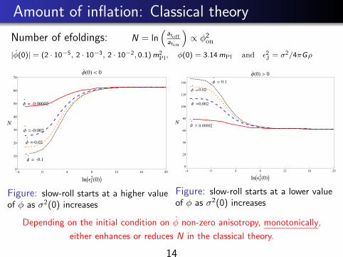
Number of efoldings: N = ln(

atoffaton

)∝ φ2on

|φ(0)| = (2 · 10−5, 2 · 10−3, 2 · 10−2, 0.1)m2Pl, φ(0) = 3.14mPl and ε2J = σ2/4πGρ

-0.002

-0.02

-0.1

-0.00002

Φ

.=

Φ

.=

Φ

.=

Φ

.=

-4 0 4 8 12 16 200

10

20

30

40

50

60

70

lnIΕJ2H0LM

N

Φ H0L < 0

Figure: slow-roll starts at a higher valueof φ as σ2(0) increases

0.002

0.00002

0.02

0.1Φ

.

=

Φ

.

=

Φ

.

=

Φ

.

=

-4 0 4 8 12 16 20

0

20

40

60

80

100

120

140

lnIΕJ2H0LM

N

Φ H0L > 0

Figure: slow-roll starts at a lower valueof φ as σ2(0) increases

Depending on the initial condition on φ non-zero anisotropy, monotonically,

either enhances or reduces N in the classical theory.

14

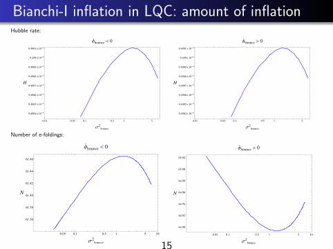
Bianchi-I inflation in LQC: amount of inflationHubble rate:

0.01 0.05 0.1 0.5 1. 5.

9.4984´10-6

9.4985´10-6

9.4986´10-6

9.4987´10-6

9.4988´10-6

9.4989´10-6

9.499´10-6

9.4991´10-6

Σ2bounce

H

Φ bounce

< 0

0.01 0.05 0.1 0.5 1. 5.

9.4984´10-6

9.4985´10-6

9.4986´10-6

9.4987´10-6

9.4988´10-6

9.4989´10-6

9.499´10-6

9.4991´10-6

Σ2bounce

H

Φ bounce

> 0

Number of e-foldings:

0.05 0.1 0.5 1. 5. 10.

61.36

61.38

61.40

61.42

61.44

61.46

Σ2bounce

N

Φ bounce

< 0

0.05 0.1 0.5 1. 5. 10.

64.90

64.92

64.94

64.96

64.98

65.00

65.02

Σ2bounce

N

Φ bounce

> 0

15

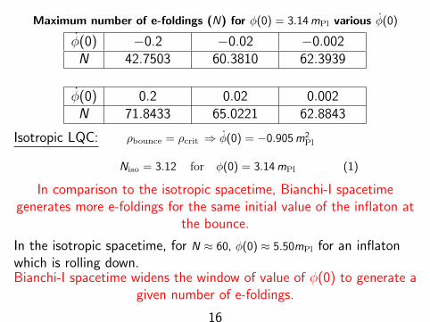
Maximum number of e-foldings (N) for φ(0) = 3.14mPl various φ(0)

φ(0) −0.2 −0.02 −0.002N 42.7503 60.3810 62.3939

φ(0) 0.2 0.02 0.002N 71.8433 65.0221 62.8843

Isotropic LQC: ρbounce = ρcrit ⇒ φ(0) = −0.905m2Pl

Niso = 3.12 for φ(0) = 3.14mPl (1)

In comparison to the isotropic spacetime, Bianchi-I spacetimegenerates more e-foldings for the same initial value of the inflaton at

the bounce.

In the isotropic spacetime, for N ≈ 60, φ(0) ≈ 5.50mPl for an inflatonwhich is rolling down.Bianchi-I spacetime widens the window of value of φ(0) to generate a

given number of e-foldings.

16

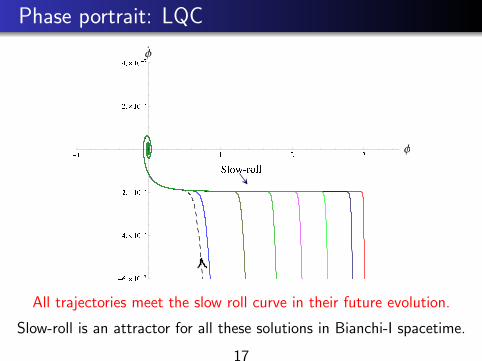
Phase portrait: LQC

All trajectories meet the slow roll curve in their future evolution.

Slow-roll is an attractor for all these solutions in Bianchi-I spacetime.

17

Summary

There are Kasner transitions across the bounce in Bianchi-Ispacetime

These transitions follow a pattern and depending on anisotropyand matter content some of them are favored- “selection rule”

Inflation takes place irrespective of the initial anisotropic shear

Anisotropy may enhance or reduce the amount of inflationdepending on the initial conditions on the inflaton velocity

Bianchi-I spacetime widens the window of the value of inflatonat the bounce, for a given number of e-foldings

18