Effective discharge analysis of ecological processes in streams

Effective discharge analysis of ecological processes in streams

Martin W. Doyle,1 Emily H. Stanley,2 David L. Strayer,3 Robert B. Jacobson,4

and John C. Schmidt5

Received 27 April 2005; revised 2 August 2005; accepted 5 August 2005; published 8 November 2005.

[1] Discharge is a master variable that controls many processes in stream ecosystems.However, there is uncertainty of which discharges are most important for drivingparticular ecological processes and thus how flow regime may influence entire streamecosystems. Here the analytical method of effective discharge from fluvial geomorphologyis used to analyze the interaction between frequency and magnitude of discharge eventsthat drive organic matter transport, algal growth, nutrient retention, macroinvertebratedisturbance, and habitat availability. We quantify the ecological effective discharge using asynthesis of previously published studies and modeling from a range of study sites. Ananalytical expression is then developed for a particular case of ecological effectivedischarge and is used to explore how effective discharge varies within variable hydrologicregimes. Our results suggest that a range of discharges is important for different ecologicalprocesses in an individual stream. Discharges are not equally important; instead, effectivedischarge values exist that correspond to near modal flows and moderate floods for thevariable sets examined. We suggest four types of ecological response to dischargevariability: discharge as a transport mechanism, regulator of habitat, process modulator,and disturbance. Effective discharge analysis will perform well when there is a unique,essentially instantaneous relationship between discharge and an ecological process andpoorly when effects of discharge are delayed or confounded by legacy effects. Despitesome limitations the conceptual and analytical utility of the effective discharge analysisallows exploring general questions about how hydrologic variability influences variousecological processes in streams.

Citation: Doyle, M. W., E. H. Stanley, D. L. Strayer, R. B. Jacobson, and J. C. Schmidt (2005), Effective discharge analysis of

ecological processes in streams, Water Resour. Res., 41, W11411, doi:10.1029/2005WR004222.

1. Introduction

1.1. Discharge Analysis in River Sciences

[2] One of the most influential paradigms of fluvialgeomorphology is that of effective discharge. Wolman andMiller’s [1960] suggestion that frequency of geomorphicprocess matters as much as magnitude of process led to theview that most fluvial landforms are shaped by frequentlyoccurring moderate floods, rather than by rare, cataclysmicfloods. Today, calculation of effective discharge is a foun-dational analysis of channel change and the estimation of in-stream flows, as well as in the burgeoning industry of riverrestoration channel design.[3] Over the past decade, ecologists have shown the

significance of flow regime in stream ecosystems. Dis-charge has been suggested to be a ‘‘master variable’’ that

limits the distribution and abundance of species [Power etal., 1995] and regulates the ecological integrity of flowingwater systems [Poff et al., 1997]. Yet despite the recognitionof the importance of discharge to both stream ecology andfluvial geomorphology, there is surprisingly little similarityin how the two disciplines have treated the effects of flowregime. Whereas geomorphologists have emphasized devel-oping explicit and quantitative relationships between dis-charge and geomorphic variables, links between ecologicalvariables and discharge tend to be less direct. Such lack ofsimilarity in approaches appears to be a key limitation inlinking the fields of geomorphology and ecology [Benda etal., 2002]. The ubiquitous application of effective dischargein fluvial geomorphology, and the need for a commonapproach to analyzing the influence of discharge on streamecosystems, suggests that the effective discharge conceptmay have relevance to allied disciplines that also study thenatural science of the river, particularly stream ecology.

1.2. Magnitude, Frequency, and Effective Dischargein Geomorphology

[4] While many interrelated variables affect stream form,discharge is the primary influence on sediment transport andchannel morphology in alluvial streams, and geomorpholo-gists have focused considerable effort on identifying howdischarge drives changes in channel form. Quantitativelylinking discharge to geomorphic processes led to the devel-opment of one of the most influential paradigms of fluvial

1Department of Geography, University of North Carolina, Chapel Hill,North Carolina, USA.

2Center for Limnology, University of Wisconsin, Madison, Wisconsin,USA.

3Institute of Ecosystem Studies, Millbrook, New York, USA.4Columbia Environmental Research Center, U.S. Geological Survey,

Columbia, Missouri, USA.5Department of Aquatic, Watershed, and Earth Resources, Utah State

University, Logan, Utah, USA.

Copyright 2005 by the American Geophysical Union.0043-1397/05/2005WR004222$09.00

W11411

WATER RESOURCES RESEARCH, VOL. 41, W11411, doi:10.1029/2005WR004222, 2005

1 of 16

geomorphology: effective discharge. Given near steadystate conditions over moderate timescales, a discharge rangecan be found which transports the most sediment given itsfrequency of occurrence. Wolman and Miller [1960] calledthis discharge the ‘‘effective discharge’’ because it accom-plished the most geomorphic work compared to other flows.Large discharges might individually transport much moresediment than smaller discharges, but are so rare that theydo not have the same opportunity for sediment transport astheir smaller counterparts. Thus Wolman and Miller sug-gested that there is a balance between the frequency andmagnitude of events, such that some moderate discharge,likely neither the largest nor the most frequent, would begeomorphologically most effective over time.[5] For actual calculation, the long-term geomorphic

effectiveness of a flood of a particular magnitude is theproduct of the effect of that flow multiplied by its frequencyof occurrence. A flow duration curve can be created usinghistoric discharge records (Figure 1), represented by f(Q)hereafter. The geomorphic effect of a given flood is deter-mined from the sediment discharge rating curve (sedimentload vs. discharge over the entire range of dischargesexperienced by the channel, curve S(Q) in Figure 1). Theproduct of the hydrologic frequency curve and the sedimentrating curve is the effectiveness curve, which represents theproportion of the total annual sediment load carried by eachincrement of discharge (E(Q) in Figure 1). The modal valueof E(Q) is then the effective discharge. Thus the effectivedischarge depends on the statistical representation of streamflows, the shape of the sediment rating curve, and thethreshold at which transport begins [Baker, 1977; Andrews,1980]. Because sediment rating curves are often stronglynonlinear [Emmett and Wolman, 2002], moderate floods(i.e., those with recurrence intervals of 1 to 5 years) tend tobe most effective for sediment transport through time. Thisrelationship is consistent over an extremely large range ofdrainage areas, channel types, and climatic regimes [Nash,1994], although there are exceptions (discussed below).[6] What intrigues most geomorphologists is the corre-

spondence between the calculated effective discharge andthe field condition of bank-full stage and bank-full dis-charge. Research subsequent to Wolman and Miller’s intro-duction of the effective discharge concept has often shownthat in alluvial channels at equilibrium with constrainingconditions, channel bank-full geometry is adjusted such thatbank-full discharge is similar to the effective discharge[Andrews, 1980; Emmett and Wolman, 2002]. That is,channels appear to adjust their geometry to allow the greatestsediment conveyance over time, although the mechanismsfor this remain unknown. Nevertheless, sediment transport isthe primary geomorphic work done by discharge in a riversystem, and there is obvious correspondence between thedistribution of work associated with sediment transport andthe work of maintaining channel form.[7] Although substantial attention is given to the dis-

charge corresponding to the mode of the effectiveness curveand to bank-full discharge, i.e., the actual value of theeffective discharge, one can take a broader view of theutility of effective discharge analysis in that it quantitativelyidentifies the range of discharges within which most sedi-ment transport occurs. That is, more generally, given adischarge-dependant function of a process, effective dis-

charge analysis is a tool with which to evaluate the range ofdischarges (e.g., baseflow or rare flood) most important forthe process of interest.

1.3. Applying Effective Discharge to Stream Ecology

[8] Many ecological processes are known to be dis-charge-dependent, such as the flux of nutrients and organicmaterial, while others have the potential to be discharge-dependent, such as macroinvertebrate drift. The utility ofeffective discharge analysis in geomorphologic analysis offluvial landforms suggests that it may be usable in aquaticecology as well. Doyle [2005] applied an effectivenessanalysis to nutrient retention in streams using a theoreticalmodeling approach and showed that the most effectivedischarges for nutrient retention are those at and belowthe modal discharge. More generally, his analysis suggestedthat effective discharge analysis was a useful tool forexamining processes other than sediment transport, partic-ularly some ecological processes.[9] Here we explore the interaction of magnitude and

frequency in ecological processes by applying effectivedischarge analysis (hereafter Qeff refers to ecological effec-tive discharge), to stream ecosystems. The goal of this paperis to explore what insight into ecological processes can begained by using the effective discharge analysis, and morespecifically, to what extent the concept is applicable to anarray of ecological variables. We suggest effective dischargeas an objective framework for examining the strength andnature of the relationship between discharge and ecologicalresponse, and how these relationships vary among differentecological variables or among different streams. We drawfrom a wide range of ecological variables using data derivedfrom previously published studies. In cases where data werenot available, modeling approaches are used. In addition, asimple modeling approach is developed to analyze Qeff forecosystem variables that can be described by a simple powerfunction to make more generalized predictions about the roleof hydrologic variability in influencing stream ecosystems.[10] In general, we use this analysis to distinguish

among ecological processes dominated by base flow

Figure 1. Components of effective discharge (Qeff).Adapted from Wolman and Miller [1960].

2 of 16

W11411 DOYLE ET AL.: ECOLOGICAL EFFECTIVE DISCHARGE W11411

(Qeff /Qmode � 1), moderate floods (i.e., recurrence intervalof years, Qeff /Qmode � 10–100), and extreme floods (i.e.,recurrence interval of decades to centuries, Qeff /Qmode �1000). These results are used to examine how particularecological variables are expected to vary spatially andtemporally, and the effect of this variation on defining Qeff

for any given ecological variable. While Qeff is shown tobe a useful tool in analyzing stream ecosystems, there areecological variables for which it is poorly suited, and weshow how to identify those variables for which thisanalysis approach is most appropriate. We close with anexamination of potential anthropogenic effects Qeff, poten-tial applications for river management, and potential futuredirections for research.

2. Methods

2.1. Analysis of Available Data

[11] Quantifying Qeff for ecosystem processes firstrequires explicit knowledge of the relationship betweensome ecological variable and discharge (curve S(Q) inFigure 1). Developing S(Q) for geomorphology is relativelystraightforward in that what matters is known; bed materialload determines channel form, and the exponential shape ofthe geomorphic work function is consistent. In contrast, anarray of ecological variables are influenced or governed tovarying degrees by discharge, but also by other processes,such as temperature, sunlight, grazing, predation, and com-petition. Also, there are positive and negative feedbacksamong ecological processes that make it more difficult toisolate the role of discharge. Thus we sought to analyze arange of response variables across different levels of eco-logical organization to provide an evaluation of possibleecological response to discharge.[12] We searched published studies that related ecological

variables directly to discharge and then analyzed these datato calculate Qeff. The analysis also requires long-termhydrologic data to develop a frequency distribution curve.With the exception of physical habitat data from incremen-tal flow methodology, relatively few ecological data setsmet both of these criteria. A subset of qualifying data setswas selected to arrive at a final list that represented the bestavailable variety of ecological variables. The variablesanalyzed are (1) organic matter transport, (2) algal growth,(3) transport of macroinvertebrates by floods, (4) nutrienttransport and retention, and (5) physical habitat availability.2.1.1. Ecological Variables Analyzed[13] At the ecosystem level, organic matter (OM) trans-

port and algal growth are core components of a stream’senergy balance and provide valuable information for under-standing food web dynamics. Nutrient transport and reten-tion also represent fundamental ecosystem attributes andretention is now a widely used metric to illustrate within-and between-system differences in nutrient cycling instreams [Fisher et al., 2004]. While several studies haverelated these variables to discharge [e.g., Fisher and Likens,1972; Webster, 1983; Butturini and Sabater, 1998], fewhave taken the next step to place these relationships in thecontext of the stream’s naturally varying discharge regime[Fisher et al., 2004].[14] Algal growth, transport of macroinvertebrates by

spates, and habitat availability provide different measures

of organismal-level responses to discharge. Understandingthe role of disturbance (most often flooding) in shapingpopulation and community dynamics has been an impor-tant research avenue in stream ecology over the pastdecade (e.g., see review by Resh et al. [1988]), but thesestudies typically emphasize either the response to individ-ual floods [e.g., Fisher et al., 1982; Imbert and Perry,2000] or the relationship between disturbance frequencyand biotic response [e.g., Townsend et al., 1997]. Our goalis to link response variables to the entire range of astream’s discharge rather than focusing exclusively onextreme events.[15] Finally, the effect of discharge variation on hydrau-

lically defined habitat availability is the most widespreadapproach used in environmental flow analyses worldwide[Tharme, 2003]. Typically, such studies employ hydraulicmodels to assess the distribution of depth, velocity, and to alesser extent, substrate and cover as functions of discharge.Ecosystem responses in terms of fish population or com-munity metrics are then related empirically to indicescalculated from the physical habitat variables [Petersonand Rabeni, 2001; Tharme, 2003]. Thus inventories ofphysical habitat (i.e., depth and velocity) known to beimportant for specific biota are used as a surrogate fordirect examination of population or community dynamics.Discharge-habitat relations, S(Q), then can be modeled tocalculate Qeff of habitat availability. The validity of thisapproach in describing habitat availability depends entirelyon how well the hydraulic units identified describe biolog-ically important habitat constraints.[16] Some ecological variables are better suited to the

effective discharge analysis than others. This limitation, andother limitations of our analytical approach are discussed atgreater length below.2.1.2. Analysis Methods[17] The same analytical methods were followed for each

variable, and specific details for the analysis are provided inthe appendices in the auxiliary material.1 Sources of eco-logical data are listed in Table 1. Hydrologic data for eachof the study sites were obtained from historic data sets, andmean daily discharge was used in all cases to develop thehydrologic frequency distribution. All hydrologic dataavailable in the records were used even though the pub-lished study may have collected ecological data for only aperiod of time within the entire hydrologic data set timeperiod. Each hydrologic data set was divided into 25logarithmically distributed bins and then the hydrologicfrequency distribution was used to compute the portion oftime the flow was within the discharge bin. This generatedf(Q) in Figure 1. Using a logarithmic distribution of dis-charge bins provides a more representative distributionfrom which to calculate the effective discharge thanarithmetically distributed bins, which underemphasizessmaller, more frequent discharges likely to be importantfor ecological processes.[18] For each of the discharge bins, the published rela-

tionship was used to link the ecological variable to thespecific discharge bin to generate the S(Q) curve, whereS(Q) represents the discharge dependence of the ecological

1Auxiliary material is available at ftp://ftp.agu.org/apend/wr/2005WR004222.

W11411 DOYLE ET AL.: ECOLOGICAL EFFECTIVE DISCHARGE

3 of 16

W11411

variable. Only relationships for S(Q) which were publishedand statistically significant were used for rating curves. Theproduct of f(Q) and S(Q) produces the effectiveness curve,E(Q), the peak of which is the ecologically effectivedischarge. Borrowing from the terminology of fluvial geo-morphology, this final curve is an expression of ‘‘ecologicalwork’’ done by flow for the target variable.[19] The first analysis is a simple case of particulate

organic matter (POM) transport data from Golladay et al.[2000] for Ichawaynochaway Creek, a fifth-order stream inGeorgia (Appendix A). Seasonal effects on loading andsubsequent transport of organic matter are often quitestrong, so a single measure of organic matter transportand discharge, as done by Golladay et al. [2000], is notsufficiently representative of temporal fluctuations that candominate organic matter dynamics in forested stream eco-systems. Thus Webster [1983] developed season-specificcoarse particulate organic matter (CPOM) rating curves forBig Hurricane Creek, a small headwater stream (�60 hadrainage area) in the Coweeta Hydrologic Laboratory inNorth Carolina. These data were used to calculate seasonspecific values of Qeff for CPOM (Appendix B).[20] Data from multiple studies [Fisher and Likens, 1973;

Meyer and Likens, 1979] from Bear Brook, New Hamp-shire, were used to investigate differences in Qeff amongorganic matter size fractions (Appendix C). DOM curvesfrom Hubbard Brook were then compared to thosederived from Sycamore Creek, Arizona [Jones et al.,1996] (Appendix D), to consider how discharge relationsfor a single variable can vary between streams with vastlydifferent flow regimes.[21] Effective discharge for solutes were investigated first

by considering differences among different solutes, then byexamining transport and retention of dissolved and partic-ulate P fractions. Qeff for NO3, PO4, and SO4 were deter-mined for Gwynns Falls at Villa Nova, Maryland (drainagearea �84 km2), from the NSF-LTER Baltimore EcosystemStudy (Appendix E). Transport and retention relationshipsfor different fractions of P were also derived from

Bear Brook, New Hampshire [Meyer and Likens, 1979](Appendix F).[22] Unlike nutrients and organic matter, we found no

long-term relationships quantitatively linking periphyton(benthic algae and associated microbial community) accu-mulation and discharge, which was needed to develop aperiphyton effective discharge curve. Thus an approximatebut realistic relationship was modeled using some availabledata and the periphyton accumulation model of Hondzo andWang [2002] and tested using periphyton and hydrologydata available for Sycamore Creek, Arizona (Appendix G).The modeled relationship provides a sense for how theeffective discharge curve for periphyton is likely to differfrom the previously developed curves.[23] To quantify the potential changes of macroinverte-

brates due to discharges, we used data from Cobb et al.[1992] relating the portion of invertebrates mobilized as afunction of discharge in Wilson Creek, Manitoba, a fourth-order stream with drainage area of 22 km2 (Appendix H).Finally, habitat-discharge relationships were developed forBear Creek in the Ozark Highlands of northern Arkansas.Habitat availability as a function of discharge was delineatedbased on the hydraulics of flow as a function of discharge,primarily by delineating the channel on the basis of Froudenumber, a dimensionless hydraulic variable (see Appendix I)[Reuter et al., 2002].[24] In cases where the ecological variable increased

monotonically as a function of discharge, we developedthe relationship between the variable and discharge accord-ing to a power function

S ¼ aQb ð1Þ

where S is the ecological variable of interest (e.g., CPOM),Q is discharge, and a and b are empirically fittedparameters. In cases where studies presented multiplerelationships (e.g., to account for hysteresis effects), thesimplest function which fit equation (1) was used. Ifrelationships were given in alternative forms (e.g., poly-

Table 1. Summary of Results of Effective Discharge Analysis

Ecological Variable Site StudyMean Daily Q,

m3/sQmode,m3/s

Qeff,m3/s

Q2,m3/s m s b

POM Ichawaynochaway Ck, GA Golladay et al. [2000] 22 15 57 144 2.8 0.8 1.5CPOM winter Big Hurricane Br, NC Webster [1983] 0.074 0.067 0.084 0.20 �2.7 0.3 1.8CPOM summer Big Hurricane Br, NC Webster [1983] 0.051 0.048 0.18 0.14 �3.1 0.4 3.7CPOM late summer Big Hurricane Br, NC Webster [1983] 0.042 0.039 0.050 0.12 �3.3 0.5 2.1CPOM leaf fall Big Hurricane Br, NC Webster [1983] 0.053 0.054 0.080 0.16 �3.1 0.5 2.2CPOM Bear Brook, NH Fisher and Likens [1973] 0.0037 0.0010 0.021 0.071 �6.8 1.9 1.3FPOM Bear Brook, NH Fisher and Likens [1973] 0.0037 0.0010 0.088 0.071 �6.8 1.9 1.4DOM Bear Brook, NH Fisher and Likens [1973] 0.0037 0.0010 0.021 0.071 �6.8 1.9 1.1CPOM Bear Brook, NH Meyer and Likens [1979] 0.0037 0.0010 0.021 0.071 �6.8 1.9 1.3FPP winter Bear Brook, NH Meyer and Likens [1979] 0.0048 0.0012 0.034 0.068 �6.1 1.1 1.4FPP summer Bear Brook, NH Meyer and Likens [1979] 0.0016 0.00042 0.045 0.027 �8.2 2.2 1.7P retention Bear Brook, NH Meyer and Likens [1979] 0.0037 0.0010 0.0010 0.071 �6.8 1.9 N/ADOC Sycamore Ck, AZ Jones et al. [1996] 0.76 0.035 73 34 �4.2 3.2 0.9Periphyton Sycamore Ck, AZ Grimm and Fisher [1989] 0.76 0.035 0.67 34 �4.2 3.2 N/ANO3 load Gwynns Falls, MD Baltimore Ecosystem Study 1.1 0.90 0.90 23 �0.4 0.8 0.7PO4 load Gwynns Falls, MD Baltimore Ecosystem Study 1.1 0.90 142 23 �0.4 0.8 1.8SO4 load Gwynns Falls, MD Baltimore Ecosystem Study 1.1 0.90 0.90 23 �0.4 0.8 0.8Invertebrate dist Wilson Ck, Manitoba Cobb et al. [1992] 0.156 0.0060 0.049 3.6 �3.2 1.7 N/APool habitat Bear Ck, AR Reuter et al. [2002] 3.0 1.8 1.8 84 �0.1 1.4 N/ARiffle habitat Bear Ck, AR Reuter et al. [2002] 3.0 1.8 3.2 84 �0.1 1.4 N/AHabitat diversity Bear Ck, AR Reuter et al. [2002] 3.0 1.8 0.41 84 �0.1 1.4 N/A

4 of 16


nomials, log space), they were converted to a powerfunction. This allowed direct comparisons among studies,and for the theoretical explorations discussed below.[25] Once an effectiveness curve was generated, the peak

of this curve was designated as the Qeff, i.e., the mosteffective discharge. Some Qeff curves had multiple modes,so the Qeff was always identified as the maximum of thecurve. Additionally, for each study we calculated the returninterval for the 2 year flood event so that the Qeff could becompared to the Q2 (i.e., 2 year flood event), since the Q2 isoften roughly comparable to the geomorphic Qeff [Wolmanand Miller, 1960; Andrews, 1980] and is a general approx-imation of the bank-full discharge. We assumed a logPearson type III frequency distribution for the annual seriesof peak flows [Stedinger et al., 1992].

2.2. Model Development

[26] We developed an analytical relationship for effectivedischarges in cases where equation (1) applied to theecological variable: all variables but periphyton accumula-tion, macroinvertebrate mobilization, and habitat availabil-ity. As a first approximation of hydrologic frequency, dailydischarge was assumed to be lognormally distributed[Stedinger et al., 1992; Nash, 1994]. The frequency of themean daily discharge is then given by:

f Qð Þ ¼ 1

Qsffiffiffiffiffiffi2p

p e� lnQ�mð Þ2

2s2 ð2Þ

where m and s are the mean and the standard deviation ofthe logarithm of discharge, respectively. The effectivenessof a given discharge, the product of f(Q) and S, is

E Qð Þ ¼ aQb

Qsffiffiffiffiffiffi2p

p e� lnQ�mð Þ2

2s2 ð3Þ

The curve generated by equation (3) is the effectivedischarge curve (i.e., curve E in Figure 1), the peak ofwhich is Qeff. The actual effective discharge can be

determined by setting the derivative of E(Q) with respectto Q equal to zero and solving for Q, which can beapproximated by [Vogel et al., 2003]

Qeff ¼ e b�1ð Þs2þm ð4Þ

This equation is applicable to any ecological variable whichcan be described using the power function and if dischargecan be described by a lognormal distribution. Note that m isthe modal discharge in ln space, and so em is the modalarithmetic discharge; m and s can also be used with well-known transformations to compute the arithmetic mean andcoefficient of variation of daily discharge at a site [Vogel etal., 2003].[27] To test this approach, values of ecological effective

discharge were computed using the standard techniquefor variables described by power functions and thevalues predicted by equation (4). The advantage of usingequation (4) is that it provides a quick approximation ofthe relative effects of hydrology (as reflected in the m ands terms) and ecology (reflected in the b term) on theapproximate range of Qeff, i.e., to rapidly approximatewhether a particular ecological variable at a site is likely tobe dominated by baseflow or rare floods.

3. Results and Discussion

3.1. Organic Matter Transport

3.1.1. Annual Organic Matter Loads[28] Qeff for POM on Ichawaynochaway Creek was

57 m3/s (Figure 2), which was approximately 3 times themean annual discharge (mean annual discharge = 21.6 m3/s;Qmode = 11 m3/s), but only a fraction of the 2 year (bank-full) flood event (144 m3/s). While floods are important inthe transport of POM, as shown by the nonlinear increasingrelationship between POM and Q (Figure 2), it is thedischarges slightly larger than the mean daily dischargethat are most effective for the export of organic matter overlong periods of time.3.1.2. Seasonal Variability[29] Seasonal variability in Qeff at Big Hurricane Branch

was limited (Table 1 and Figure 3): Qeff varied from 0.05m3/s in the late summer to 0.18 m3/s in the early summer.While the winter had the highest mean daily discharge(0.074 m3/s), it also had a relatively low exponent for thedischarge-CPOM rating curve: the exponent b in equation(1) was 1.8 whereas all the other seasons had rating curveexponents greater than 2.1, with the early summer havingthe highest exponent of 3.7. In addition, while a narrowrange of discharges was relatively effective for CPOMtransport during the winter, a much wider range of flowswas effective in other months, particularly during the earlysummer.[30] Effective discharge for organic matter loads is deter-

mined jointly by the distribution of flows, the relative easewith which organic matter is transported by those flowswithin each season, and the availability of organic matter fortransport. Webster [1983] suggested that in early summer,CPOM is more easily transported as it has been brokendown over the winter (ease of entrainment) since initial leaffall, resulting in the higher value for b in the early summerthan in other months. Early summer months had a much

Figure 2. Effective discharge for particulate organicmatter (POM) on Ichawaynochaway Creek, Georgia. Dataare from Golladay et al. [2000].


5 of 16

W11411

lower mean daily discharge than winter months, but thiswas compensated for by relatively large values for theexponent b, indicative of increased effectiveness of dis-charges during summer for the transport of CPOM. During

winter months, formation of large leaf packs (high thresholdof entrainment) limited the transport of CPOM despite thehigher discharges during this season [Webster, 1983]. ThusCPOM transport in Big Hurricane Creek shows the discrep-ancy between the frequency of storm events (highestdischarge in the winter months), and the magnitude ofecological work in the form of organic matter transportdone by these events.3.1.3. Effect of Organic Matter Size Fractions and Site[31] As expected, Qeff varied for the different size frac-

tions of organic matter in Bear Brook: 0.021 m3/s forCPOM and DOM, and 0.088 m3/s for FPOM (Figure 4and Table 1). For comparison, the mean daily discharge andQmode are 0.0037 and 0.001 m3/s, respectively, and the Q2

for Bear Brook is 0.071 m3/s (Table 1). Thus the most

Figure 3. Variation in interseason effective discharge forcoarse particulate organic matter (CPOM) on Big HurricaneBranch, Georgia. Data are from Webster [1983].

Figure 4. Variation in effective discharge among sizefractions of organic matter on Bear Brook, New Hampshire,including coarse particulate organic matter (CPOM), fineparticulate organic matter (FPOM), and dissolved organicmatter (DOM). Data from Fisher and Likens [1973].

6 of 16


effective discharge for all forms of organic matter in BearBrook is moderate flood flows.[32] In contrast to Bear Brook, Qeff for DOC in Sycamore

Creek, Arizona, was 73 m3/s, which was substantially largerthan the Qmean (0.76 m3/s) and Qmode (0.035 m3/s) (Figure 5and Table 1). Whereas moderate flows were most effectivefor DOM at Bear Brook, very large and infrequent floodswere most effective for DOC transport at Sycamore Creek(Figure 5 and Table 1). Indeed, the most effective dischargefor DOC transport in Sycamore Creek was �2000 timesgreater than the modal discharge, whereas Qeff for DOMwas within an order of magnitude of Qmode for Bear Brook.

3.2. Nutrient Dynamics

3.2.1. Differences Among Solutes[33] The Qeff for PO4 loads differed from those for NO3

and SO4 loads in Gwynns Falls, MD (Figure 6 and Table 1).Qeff for both NO3 and SO4 loads was the same as the modaldaily discharge, 0.9 m3/s. Thus the modal discharge dom-inates the transport of NO3 and SO4 in this system.However, PO4 transport was dominated by large discharges:the Qeff was the largest flow of record, 142 m3/s. Thesecondary mode in the Qeff curve for PO4 suggests that21 m3/s was also a highly effective discharge for thetransport of PO4. For comparison, Q2 at this site is 23 m3/s.3.2.2. Measures of P Cycling[34] Meyer and Likens [1979] showed that net phospho-

rus retention (portion of dissolved phosphorus retained) wasinversely related to discharge, among other variables. Thatis, as discharge increased, less dissolved phosphorus wasretained in their study reach; other studies have shownsimilar relationships [e.g., Butturini and Sabater, 1998;Doyle et al., 2003]. Thus the fundamental relationshipbetween this ecological variable (P retention) and Q issubstantially different than for the previous cases.[35] The most effective discharge for net phosphorus

retention in Bear Brook was 0.001 m3/s (Figure 7 andTable 1), which was comparable to the Qmode (0.001 m3/s).This was also comparable to theQeff for DOM at Bear Brook,but an order of magnitude less than the Qeff for CPOM or

FPOM (Figure 4 and Table 1). Thus frequent, low flows weremost effective for net phosphorus retention in Bear Brook(see detailed discussion of effective discharge for nutrientretention by Doyle [2005]), which likely reflected greateropportunity for biotic uptake as well as greater sediment-water contact that fosters sorption of P on sediment surfaces.[36] Meyer and Likens [1979] also quantified P export,

which was predominantly in the form of fine particulatephosphorus (FPP). FPP transport was dominated by mod-erate flood flows: 0.034 m3/s for Qeff in the winter and0.045 m3/s in the summer (Figure 7 and Table 1). Thesedischarges are 1 to 2 orders of magnitude greater than the

Figure 5. Effective discharge for dissolved organic carbon(DOC) on Sycamore Creek, Arizona. Data are from Jones etal. [1996].

Figure 6. Effective discharge for nutrient loads onGwynns Falls, Maryland. Data are from Baltimore Ecosys-tem Study [Groffman et al., 2004].


7 of 16

W11411

modal discharge, and indicate that moderate floods are mosteffective at transporting FPP out of Bear Brook, driving thelong-term FPP export budgets. Thus there were essentiallytwo effective discharges for phosphorus dynamics in BearBrook. Low flows dominate the accumulation or short-termretention of phosphorus, whereas moderate flood flowsdominate the export of phosphorus. Meyer and Likens alsoshowed that dissolved phosphorus retention in Bear Brookis temporary; over longer timescales the inputs and outputsof phosphorus balance. They showed that dissolved andcoarse particulate phosphorus were the dominant inputs ofphosphorus which were retained in the study reach, and our

analysis shows that retention of these forms of P primarilyoccurred at low flows. Dissolved and coarse particulatephosphorus were converted into fine particulate phosphorus(FPP) over time, and that FPP made up the bulk of theexported phosphorus from Bear Brook [Meyer and Likens,1979]. Thus both ranges of discharges were necessary forthe current balanced P budget at Bear Brook.

3.3. Periphyton Growth and Removal

[37] The effective discharge for periphyton accumulationin Sycamore Creek, Arizona (0.67 m3/s) was greater thanthe modal discharge, but almost the same as the mean dailydischarge (0.76 m3/s, Table 1 and Figure 8). For this desertstream, a wide range of discharges have comparable fre-quencies, leading to a relatively large difference between themodal discharge and the mean daily discharge (Table 1).This analysis also shows that there is a relatively limiteddischarge range that allows the greatest accumulation ofperiphyton on the channel bed: relatively small amounts ofperiphyton are accumulated at low discharges, but at largedischarges, which occur infrequently, periphyton is re-moved via scour. This is in contrast to organic matter ornutrient loads in that while they have similar rarity of highflows, these loads are elevated at high flows rather thanreduced.[38] This value for Qeff for periphyton is in stark contrast

with the effective discharge for DOC of 73 m3/s (Figure 5and Table 1) at Sycamore Creek. This suggests that, likeshown for Bear Brook, multiple discharges are effective forvarious ecological variables; low flows for periphytonaccumulation in Sycamore Creek, high flows for DOCtransport.

3.4. Macroinvertebrate Disturbances

[39] Unlike the earlier measures, the effective dischargecurve for macroinvertebrate mobilization was distributedover a wide range of discharges, and slightly bimodalin Wilson Creek, Manitoba (Figure 9 and Table 1). Themost effective discharge for invertebrate mobilization was

Figure 7. Effective discharge for dissolved phosphorus(P) retention and fine particulate phosphorus (FPP) transporton Bear Brook, New Hampshire. Data are from Meyer andLikens [1979].

Figure 8. Effective discharge for periphyton growth andremoval on Sycamore Creek, Arizona. Data are generatedby simulation model, and calibration data are from Grimmand Fisher [1989].

8 of 16


0.049 m3/s, although there was a secondary mode in theeffective discharge curve at 0.156 m3/s. Thus the Qeff wasalmost an order of magnitude larger than the Qmode. Thisindicates that for Wilson Creek, a wide range of dischargesare similarly effective in controlling the disturbance ofinvertebrates over time and that moderate floods are mosteffective at mobilizing macroinvertebrates.

3.5. Physical Habitat Availability

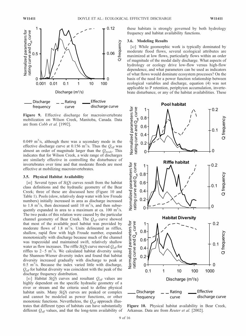
[40] Several types of S(Q) curves result from the habitatclass definitions and the hydraulic geometry of the BearCreek; three of these are discussed here (Figure 10 andTable 1). Pools (slow, relatively deep water with low Froudenumbers) initially increased in area as discharge increasedto 1.8 m3/s, then decreased until 10 m3/s, and then subse-quently expanded in area to a maximum at ca. 100 m3/s.The two peaks of this relation were caused by the particularchannel geometry of Bear Creek. The Qeff curve showedthat most of the available pool habitat was provided bymoderate flows of 1.8 m3/s. Units delineated as riffles,shallow, rapid flow with high Froude number, expandedmonotonically with discharge because much of the channelwas trapezoidal and maintained swift, relatively shallowwater as flow increases. The riffle S(Q) curve moved Qeff forriffles to 2–5 m3/s. We calculated habitat diversity usingthe Shannon-Wiener diversity index and found that habitatdiversity increased gradually with discharge to peak at0.5 m3/s. Because the index varied little with discharge,Qeff for habitat diversity was coincident with the peak of thedischarge frequency distribution.[41] Habitat S(Q) curves and resultant Qeff values are

highly dependent on the specific hydraulic geometry of ariver or stream and the criteria used to define physicalhabitat units. Many S(Q) curves are peaked or complexand cannot be modeled as power functions, or othermonotonic functions. Nevertheless, the Qeff approach illus-trates that different types of habitats can have substantiallydifferent Qeff values, and that the long-term availability of

these habitats is strongly governed by both hydrologyfrequency and habitat availability functions.

3.6. Modeling Results

[42] While geomorphic work is typically dominated bymoderate flood flows, several ecological attributes aremaximized at low flows, particularly flows within an orderof magnitude of the modal daily discharge. What aspects ofhydrology or ecology drive low-flow versus high-flowdependence, and what parameters can be used as indicatorsof what flows would dominate ecosystem processes? On thebasis of the need for a power function relationship betweenecological variables and discharge, equation (4) was notapplicable to P retention, periphyton accumulation, inverte-brate disturbance, or any of the habitat availabilities. These

Figure 9. Effective discharge for macroinvertebratemobilization on Wilson Creek, Manitoba, Canada. Dataare from Cobb et al. [1992].

Figure 10. Physical habitat availability in Bear Creek,Arkansas. Data are from Reuter et al. [2002].


9 of 16

W11411

variables would need to be modeled with forms of S(Q)other than a power function and examples are discussedbelow.[43] Despite the generality of equation (4), predicted

values of Qeff matched the observed values fairly well,although there were outliers (PO4 loads at Gwynn’s Fallsand DOC load at Sycamore Creek) for which the actual Qeff

was much greater than that predicted. However, the analyt-ical expression (equation (4)) captured the main features ofthe effective discharge observed: all other predicted valuesof Qeff were within an order of magnitude of the observedQeff (Table 1 and Figure 11, p < 0.01, R2 = 0.90).[44] Equation (4) reveals several interesting aspects of

ecological effective discharge. First, the coefficient a doesnot appear in the equation, thus indicating that it is thedegree of nonlinearity, expressed in exponent b, that con-trols the effective discharge. Second, this equation allowsone to assess the necessary conditions for effective dis-charge to be near low, frequent discharges (Qeff � Qmode)or near rare floods (Qeff � Qmode). A limiting case occursfor an ecological variable that varied linearly with dis-charge, i.e., if the exponent b were 1. As b ! 1, then byequation (4), Qeff ! em, or Qeff ! Qmode. Thus, forecological processes that vary approximately linearly withflow, the most effective discharge can be approximatedby the modal discharge. As b increases beyond 1, thenQeff > Qmode, and if b < 1 then Qeff < Qmode. For progres-sively larger values of jb � 1j, the Qeff is essentially‘‘pulled’’ away from Qmode, toward larger discharges ifb > 1, and toward smaller values if b < 1.[45] As examples, the exponent b for NO3 and SO4 load

curves for Gwynn’s Falls were less than, but close to 1,

while the b exponent for PO4 was 1.8. Correspondingly, theQeff for NO3 and SO4 was the same as Qmode, while Qeff forPO4 was orders of magnitude larger than Qmode (Figures 6and 12). The exponents for CPOM and FPOM at Bear Brookwere 1.3 and 1.4, respectively, and all of the associatedeffective discharges were closer to moderate flood eventsthan to the mean or modal discharge (Figures 4 and 12).Thus small changes in the b exponent can result in substan-tial changes in Qeff. Coming back to sediment loads in riverchannels, exponents relating gravel sediment loads to dis-charge are often in the range of 2.3 to 5.1 [Emmett andWolman, 2001], so effective discharge for gravel transport ismost often associated with the 1.5+ year flood event, i.e.,Qeff � Qmode.

4. General Discussion and Synthesis

[46] The concept of effective discharge has considerablepotential to aid in the analysis and management of streamecosystems, just as it has in geomorphology [e.g., Shields etal., 2003]. Even for the simplest cases of ecologicalresponse to discharge (i.e., monotonically increasing,POM or nutrient loads), the high error in the relationshipbetween the ecological variable and discharge will lead tohigh error in the estimates of Qeff [Benda et al., 2002].Further, the application of effective discharge analysis inecology will be more complex than in geomorphology, andthe patterns of effectiveness curves will vary both acrossecological variables and ecosystems. Nevertheless, the con-ceptual and analytical utility of the effective dischargeanalysis allows us to explore several general questionsabout how hydrologic variability influences various ecolog-

Figure 11. Theoretically derived Qeff and observed Qeff for ecological parameters that can be describedby a power function. Thick diagonal line indicates theoretically predicted equals observed; other linesindicate one order of magnitude discrepancies between predicted and observed.

10 of 16


ical processes in streams. Given the uncertainty associatedwith the data contributing to the meta-analysis, the discus-sion below is focused on identifying the general range offlows that are most effective for a particular ecologicalvariable rather than attempting to quantify a specific mag-nitude of flow that will dominate all ecological processes,i.e., identify what types of flows (extreme floods or com-mon base flows) are most important for different ecologicalvariables.

4.1. Single or Multiple Effective Discharges?

[47] The synthesis of the previous studies suggests thatseveral discharges can be expected to be ecologicallyeffective for a given stream (Figure 12). For example, theanalysis of the Bear Brook data for phosphorus showed thatboth low flows and moderate floods maintained the phos-phorus budget, with low flows dominating P retention andmoderate floods maintaining the output, as FPP. In theabsence of floods, then there may be a net accumulationof phosphorus, whereas chronic flooding may result in adepletion of P. Thus both ranges of discharges are necessaryto maintain long-term nutrient balance [Reddy et al., 1999].[48] Across multiple sites, some ecological variables are

driven by base flows or mean daily discharge (e.g., periph-yton accumulation at Sycamore Creek, NO3 or SO4 loads atGwynns Falls) while others primarily driven by moderateflood flows (e.g., CPOM export; PO4 loads at GwynnsFalls). Thus, rather than a single effective discharge peak

wherein a relatively narrow range of discharges dominatesmany processes, certain ecological processes are dominatedby base flows (Qeff /Qmode � 1; e.g., NO3 loads, periphytonaccumulation, Bear Creek pool availability), others bymoderate floods (Qeff /Qmode � 100; e.g., Bear BrookCPOM, Bear Creek riffle availability), while others drivenby rare, extreme floods (Qeff /Qmode � 1000; e.g., SycamoreCreek DOC). The entire range of discharges will contributeto ecological change, with certain ecological variables beingmost influenced by particular portions of the hydrologicregime.[49] It is particularly intriguing that there were differences

in the types of flows that dominated the same variable atdifferent sites. For instance, DOC was dominated by large,rare floods at Sycamore Creek, whereas DOM was domi-nated by only moderate, frequent floods at Bear Brook. Thisdifference in Qeff likely reflects contrasting sources of DOCat these two sites. DOC transport in Sycamore Creek isdominated by terrestrial inputs during flash floods and thedominance of extreme flows suggests an unusually highexport of catchment NPP [Jones et al., 1996]. Arid con-ditions limit both transport and decomposition of terrestrialOM, such that when a sufficiently large storm is finally ableto move this material to the stream, the available terrestrialpool is substantial and thus results in high DOC concen-trations and loads during the associated flood. In contrast,OM decomposition is an ongoing process in the mesicsetting of Bear Brook, NH. Groundwater discharge and

Figure 12. Relative values of Qeff compared to Qmode. Thick horizontal line indicates Qeff values equalto Qmode. References are as follows: 1, Golladay et al. [2000]; 2, Meyer and Likens [1979]; 3, Fisher andLikens [1973]; 4, Webster [1983]; 5, Grimm and Fisher [1989]; 6, Jones et al. [1996]; 7, Cobb et al.[1992]; 8, Baltimore Ecosystem Study (L. Band and P. Groffman, personal communication, 2004);9, Reuter et al. [2002].


11 of 16

W11411

slow decomposition of allochthonous OM provide a rela-tively constant source of DOC to this system, resulting inlow-flow and moderate flood dominance.[50] Results also indicate that high flows play a critical

role in maintaining some ecological functions in streams.Discharges just at or above the bank-full discharge willlikely be highly effective for an array of processes becausethese flows access the floodplain, increasing ecologicalprocesses associated with the capture of these additionalhabitats. Some examples include the addition of habitat forfish and phosphorus retention in alluvial floodplain rivers[Welcomme, 1979; Olde Venterink et al., 2003]. Further,discharges that create boundary shear stresses near thecritical value for sediment mobilization are also likely tobe effective for several ecological processes, particularlyrejuvenating in-channel habitat and disturbing macroinver-tebrate communities [Townsend et al., 1997].[51] Thus effective discharge analysis provides a quanti-

tative and mechanistic reinforcement of previous studieswhich emphasize the importance of hydrologic variability instreams [e.g., Poff et al., 1997] and large rivers [Jacobsonand Galat, 2005; Power et al., 1995]. That is, to maintainecological function in streams, an entire range of dischargesis needed. In cases where flow is highly regulated, under-standing of effective ecological discharges can provide abasis for target discharge regimes. In another sense, this isthe danger of effectiveness, as some may see this as a callfor one discharge when a wide range is needed. We willreturn to the potential applications of Qeff below.

4.2. Types of Ecological Response to Discharge

[52] Our analysis suggests that the idea of effectivedischarge is useful in ecology, but empirical data arecurrently too scarce for us to describe all of the conditionsunder which this approach is applicable, or to lay out all ofthe possible functional relationships between discharge andecological variables. Nevertheless, it is possible to sketchout the likely potential of effective discharge analysis instream ecology.[53] Discharge plays at least four distinct roles in stream

ecosystems: material transport, habitat definition, processregulation, and disturbance. Each of these roles generates itsown set of functional relationships with discharge, whichdetermine the suitability and nature of effective dischargecurves (Table 2 and Figure 13). Some of these rolesgenerate essentially instantaneous relationships with dis-

charge, while others are highly contingent, depending onpast flow conditions, life history of organisms, or persistingconditions for some time into the future. Effective dischargeanalysis will perform well when there is a unique, essen-tially instantaneous relationship between discharge and anecological process, and poorly when the discharge historyhas lags or legacy effects.4.2.1. Discharge as Transport Mechanism[54] Transport includes both particles and solutes. Particle

concentrations (e.g., mass/volume) typically rise sharplywith rising discharge, as water velocity and thus its com-petence to move particles rises. Hence particle load (mass/time) typically rises with discharge as a power function withan exponent b > 1, creating effective discharge greater thanmodal discharge (Figures 13a–13c). This is the basis of thegeomorphic approach to effective discharge analysis, andseems to translate well to particle-associated materials inecology (Figures 2–5 and 7). Two complications arise whenconsidering the transport of particles in ecology. First, asseen in the case of CPOM (Figure 3), some groups ofparticles of ecological interest are very heterogeneous, andmay have different transport properties in different times orplaces. Effective discharge analysis will be most useful insuch cases if site- or season-specific information on particletransport can be obtained (e.g., Figure 3). Second, thegeomorphic approach to particle transport assumes aninfinite supply of particles and that sediment load istransport limited. If the particle pool is finite, i.e., supplylimited, then the rating curve for particle transport maysaturate (Figure 13e) or even decline at high discharge asthe pool of transportable particles is exhausted [e.g., Creedet al., 1996]. In such cases the concept of effectivenessremains applicable, but one cannot assume a simple mono-tonically increasing transport function.[55] In the absence of anthropogenic alterations, most

solutes arise from atmospheric sources or from weatheringin the watershed. High runoff and commensurate highstream discharge usually mean less contact time betweenthe water and soils in the watershed, so concentrations ofmany solutes arising from the watershed decline with risingdischarge. This produces a rating curve for solute load thatfollows a power function with an exponent b that is slightlyless than 1 (Figures 13a and 13b), and an effective dischargecomparable to the modal discharge. Alternatively, if thesolute originates from atmospheric deposition and is con-sumed by reactions in the watershed or stream channel (e.g.,

Table 2. Types of Ecological Response Variables to Discharge

Ecological Response to Discharge Description Examples

ExampleEffectiveness

Curvesa

Applicabilityof Qeff

AnalysisApproach

Transport Discharge has primary and directeffect on these variables.

organic matter,nutrients, particles

13a–13c and 13e high

Habitat Discharge alters flow conditions forcertain organisms and overall habitat size.

depth and velocity of flow 13f and 13h high

Process modulation Discharge indirectly regulates thesevariables and thus is correlated with them,but it is not a direct, deterministic link.

periphyton production,bivalve filtration,access to floodplain

13d, 13f, and 13g moderate

Disturbance Discharge is a reset mechanism. macroinvertebratemobilization

13f low

aEffectiveness curves refers to the hypothetical curves in Figure 13.

12 of 16


H+ and sometimes NO3�), lower contact times lead to

concentrations that rise with discharge. The rating curvefor transport load of these substances will have b > 1, andeffective discharge will be greater than modal discharge(Figure 13c). Again, functional relationships may deviatefrom these ideals if limited supplies are exhausted at highdischarge. On the basis of what is known about particle andsolute transport in streams, and on the empirical analysespresented in this paper, effective discharge analysis will be auseful tool for the analysis of material transport in streams.4.2.2. Discharge as a Regulator of Habitat[56] Discharge defines the amount and character of

habitat available in a stream by determining the size andlocation of the wetted volume, and the current speedsthroughout that wetted volume. Analysis of ecologicaleffective discharges requires knowing the function relatingdischarge to the amount or quality of habitat in the stream.Such functions may be unimodal or monotonic, but willcertainly be idiosyncratic, depending on the site-specificdetails of channel morphology, as well as the needs of theorganism. If such site-specific information is available,effective discharge analysis of habitat availability canproduce useful insights. For instance, if the habitat-discharge function S(Q) goes to zero at any value of Q,then the population will be extirpated or move elsewhere ata frequency equal to the return interval of that or moreextreme flows. This estimate can then be compared with thecolonization abilities of the species to assess the long-termviability of the population given a flow regime. Further, thearea under the effective habitat curve E(Q) provides anintegrated measure of the goodness of the habitat given aflow regime. This measure could be used, for example, to

assess the habitat value of various proposed flow regimes ata site.[57] Effective discharge analysis will not work well to

assess habitat if the organism is relatively immobile (e.g.,rooted plants, mussels). The habitat requirement for animmobile organism is that a given area of stream be suitableat all discharges. Identifying and quantifying such areasrequires information on the spatial arrangement of habitatsuitability at every probable discharge, and thus a moresophisticated approach than effective discharge analysis.4.2.3. Discharge as a Process Modulator[58] Many ecological processes are regulated by dis-

charge, either because they are regulated by current speedor by the accessibility of certain parts of the channel (e.g.,the floodplain). Rising current speeds increase turbulenceand thin boundary layers around solid objects, often stim-ulating processes such as nutrient uptake, primary produc-tion, and decomposition [e.g., Hondzo and Wang, 2002].Because current speed at a site rises with discharge as apower function with an exponent b � 0.4 and ecologicalprocesses rise with current speed linearly or less thanlinearly (i.e., b � 0), such current-sensitive functions mightbe expected to follow power functions against dischargewith exponents b � 0.3–0.5. In such cases, the ecologicallyeffective discharge would be slightly less than but compa-rable to the modal discharge (equation (4)).[59] Ecological processes may have other functional rela-

tionships with current speed. For instance, filtration rates ofactive suspension feeders such as bivalves are expected tofollow a humped curve that peaks at intermediate currentspeeds [Wildish and Kristmanson, 1997]. This relationshipwill pull the ecologically effective discharge slightly below

Figure 13. Hypothetical response curves for a variety of ecological variables. For potential ecologicalvariables, see Table 2 and discussion in text.


13 of 16

W11411

or above the modal discharge, depending if the optimalcurrent speed is less than or greater than the current speedat the modal discharge, respectively (Figure 13h).[60] If ecological processes occur chiefly in a particular

part of the channel, then there may be a threshold relation-ship between that process rate and discharge, as the wateraccesses that part of the channel. As discussed earlier, manyprocesses (e.g., P retention in large rivers [Olde Venterink etal., 2003] and spawning of many fish species [Welcomme,1979]) occur chiefly on the floodplain. Such floodplain-dependent processes will have very steep ecological effec-tiveness curves, with effective discharges shifted far abovemodal discharges (Figure 13f).4.2.4. Discharge as a Disturbance[61] Finally, discharge is an agent of disturbance that

affects many ecological variables. Disturbance (the removalof living biomass from a population) by high flows likelyfollows a steep power function (b > 1) or sigmoid curve(Figures 9, 13c, and 13e). In either case, the effectivedischarge (the one that kills or entrains the most organismsover the long term, given a flow regime) will be displacedwell above the modal discharge. The effective discharge fordisturbance may be a key discharge for understanding theeffects of disturbance on the distribution and evolution ofa species, as well as representing the outcome of evolu-tionary adaptations against disturbance. It also may be theappropriate discharge at which to look at issues like thespatial patterning of disturbance effects [e.g., Strayer,1999].[62] Two additional insights emerge from a effective

discharge analysis of disturbance. First, if the populationis small, a population will disappear if the disturbance(mortality) curve reaches any value mq such that

N 1�mq

� �< Ncrit ð5Þ

where N is the population size before the disturbance, mq isthe mortality imposed by the disturbance, and Ncrit is theminimum viable population size. Second, the populationcannot persist if the summed mortality from disturbance isgreater than the maximum achievable population growthrate in nature. Without considering the sequence of flows(see below), the population will disappear ifZ

S Qð Þf Qð ÞdQ > l ð6Þ

where l is the maximum achievable population growth ratein nature. Note that the population may not persist even ifthis condition is not met because of mortality from othersources (e.g., predators) or because population growth ratesare below optimal.[63] Very low flows may also represent an important

ecological disturbance. Again, it seems likely that thefunctional relationship will be a steep power curve (but thistime with b � 0) or reverse sigmoid curve, so that effectivedischarges fall well below modal discharges.[64] Nevertheless, important effects of disturbance on

stream ecosystems often persist for a very long time afterthe disturbance event [Romme et al., 1998]. For example,extreme floods may result in physical or biological statechanges that reorganize the system and reshape fundamentalrelationship between ecological processes and discharge.

Effective discharge analysis will not be suitable for address-ing the persistent effects of disturbance, because currentecological conditions depend so strongly on the past se-quence of flow events and ecological responses, not simplythe instantaneous discharge. Likewise, it is not prudent tointerpret the area under the effective disturbance curve asthe total mortality induced by a flow regime, because actualmortality will depend on the timing and sequence of flows,not simply on the distribution of flows.

4.3. Spatial Predictions and Effects ofLand Use Change

[65] In addition to analyzing the relative effective dis-charges of ecological processes at a particular site, thisanalysis allows qualitative predictions of how effectivedischarge should vary systematically through a watershedand the potential effects of climate or land use change. Thisis easily done by using equation (4) and the hydrologicmetrics of m and s to quantify hydrologic variability(Table 1). For example, Ichawaynochaway Creek is afourth-order river in the southeastern US (Georgia), withm = 2.8 (Qmode = 20 m3/s) and s = 0.8. In contrast, BearBrook is a second- and third-order stream in the northeasternUS (New Hampshire) with m = �6.8 (Qmode = 0.001 m3/s)and s = 1.9, indicating the smaller mean and greatervariability associated with headwater catchments. SycamoreCreek (Arizona) is a fourth-order arid stream with m = �4.2(Qmode = 0.035 m3/s) and s = 3.2, indicating the relativelylow mode but high variability associated with large, aridwatersheds.[66] Small changes in s can have a relatively large impact

on Qeff since s is squared in equation (4). Equation (4)suggests that for b > 1, s increases will result in Qeff

increases. Thus, for a given modal discharge, streams withflashy hydrology will have greater Qeff than those with lessflashy hydrology. On the basis of this logic, effectivedischarges should be skewed toward higher discharges inurban and arid watersheds. Second, equation (4) allowsapproximating systematic variability in Qeff through awatershed. Within a physiographic region, m and s are ofteninversely related [Vogel et al., 2003]; upstream rivers havesmaller discharges than downstream rivers (mupstream <mdownstream), but upstream, smaller rivers have greater hydro-logic variability than downstream, larger rivers (supstream >sdownstream). Therefore, for a given value of b, Qeff in largerchannels will be associated with more frequent, mean dis-charges than in smaller, headwater channels.

4.4. Limitations of Approach

[67] While the effective discharge concept has enjoyedmuch success in fluvial geomorphology, it has some critics.There is a continued debate on the role of extremely largefloods on dominating channel morphology [Phillips, 2002]and long-term sediment loads [Vogel et al., 2003]. Further,many geomorphologists object to the inherent assumptionof geomorphic equilibrium in applying the effective dis-charge concept [Richards, 1999]. Despite this, the impor-tance of the effective discharge concept as a cornerstone ofcurrent geomorphic thinking cannot be ignored [Doyle andJulian, 2005], nor can its use as a widely applied analyticaltool, particularly in the burgeoning field of river restoration[Shields et al., 2003].

14 of 16


[68] Unlike the case of geomorphology where sedimentrating curves can be generalized as power functions, manyecological variables lack direct relationships to discharge,and in cases where ecological variables can be linked todischarge, standard errors of prediction are often large.Rating curves can vary from highly significant to completelyinsignificant, and many studies have shown hydrologicparameters other than discharge magnitude to be highlyinfluential for stream ecosystems [Poff et al., 1997]. Finally,in the case of solute transport, while a positive relationshipbetween discharge and a response variable (e.g., PO4 reten-tion) provides useful information about that solute, it isimportant to recognize the limitations on this information. Apositive discharge-retention relationship does not identifythe specific processes at work (for example, whether PO4 isretained by biotic uptake or sorption), and it speaks to onlyone phase of the element’s cycle. Further, it is informationabout just one part of the larger solute cycle and that otherparts of the cycle may be controlled by processes that arenot discharge-dependent. Therefore these relationships em-phasize movement and storage of particular forms of asolute, and not the entire element cycle. However, theeffective discharge concept remains a highly useful ana-lytical tool that explicitly and quantitatively couples eco-system processes with hydrologic variability. In addition toproviding the broad hydrologic context for examiningecological variables, this approach draws explicit attentionto the strength and shape of the relationship betweendischarge and the response variable of interest. From apractical perspective, the modeling results presented aboveshow that Qeff is highly dependent on the b value. Theserating curves are strongly influenced by extreme events,which are often not well represented in many samplingprograms. A single extreme event may shift the b from <1,(Qeff � Qmode) to b � 1 (Qeff � Qmode). Thus failure tocapture these extremes could lead to misunderstanding theeffect of discharge on the ecological variable [Phillips,2002; Vogel et al., 2003].

4.5. Future Research Directions and Applications

[69] While the above analysis and modeling exerciseprovided intriguing results, they are not a sufficient testof the ecological effective discharge concept. Rather, asystematic evaluation of the concept at a single site for arange of ecological variables is needed. Our ability toconfidently generalize our results was reduced by ourhaving to use other studies’ data, as well as the extremediversity in study site hydrology. Applying the conceptat a particular site across a range of ecological variablesat that site would provide a more robust test of theviability of the approach for stream ecosystem analysis,followed by a similar study across a range of hydrologicvariability. Alternatively, a single ecological variablecould be examined across a range of hydrologic con-ditions. Indeed, this latter test could be easily conductedusing the National Water Quality Assessment databasethrough the U.S. Geological Survey in order to examinehow Qeff for nutrient loads varies across a wide range ofconditions.[70] There is also the intriguing potential application of

the effective discharge concept to river management issues,to include other key ecological drivers, and to other ecosys-

tems. This analysis approach would be particularly useful incomparing the long-term effects of flow modification, flowallocation, or channel reconfigurations for habitat restora-tion. For instance, on the lower Missouri River, habitat forthe endangered pallid sturgeon (Scaphirhynchus albus) islimited by a combination of channelization and flow regu-lation. Altering channel morphology alone would alter thehabitat-discharge rating curve, whereas altering dischargereleases from upstream would affect the frequency distribu-tion of flows, and a recent study analyzes the individual andcombined effects of morphology and hydrology on lowerMissouri River habitat availability [Jacobson and Galat,2005]. The relative impacts of both of these on long-termhabitat availability could be quantified using the Qeff anal-ysis. Channel and discharge could then be modified tooptimize the expected habitat availability.[71] While discharge is a master variable in streams,

ecological patterns and processes are clearly affected bymultiple drivers in addition to flow. For example, temper-ature also plays a central role for growth and life historyattributes of many aquatic organisms [Vannote and Sweeney,1980] and is often incorporated into process rate equations.In addition, other ecosystems are driven by disturbancesanalogous to floods in streams [Fisher and Grimm, 1991].Thus, if a frequency distribution can be estimated for thedisturbance of interest, and the relative amount of ecologicalwork done by that disturbance magnitude can be estimated,then the same frequency magnitude analysis could beapplied. Other salient examples might include ice stormsor landslides in forested ecosystems.

5. Conclusions

[72] Over the past decade, ecologists have made greatstrides in understanding the fundamental importance ofdischarge in shaping ecological pattern and process instreams [Power et al., 1995; Poff et al., 1997]. Yet ourunderstanding of the relationships between hydrology andecological response tends to be qualitative and descriptivein nature [Benda et al., 2002]. As both hydrologists andecologists assist in environmental decision making, quanti-tative tools become increasingly necessary. Ecologists willlikely be called upon to be specific and predictive aboutecological response to management actions in the future,particularly as unique and sizable restoration opportunitiesarise (e.g., Missouri River restoration, Grand Canyon ex-perimental floods, restoration of flows to the Everglades).[73] Attributing many ecological processes to discharge

regime is obviously a conceptual leap. Despite this, identi-fication of the effective discharge is a powerful tool foranalyzing stream ecosystems as it provides a quantitativemechanism of analyzing the combined effects of ecologicalprocesses and hydrologic variability.

[74] Acknowledgments. This study was possible because of the dataavailable through the NSF LTER Network Web sites, specifically HubbardBrook, Baltimore Ecosystem Study, and Coweeta, as well as the SycamoreCreek Ecosystem Study. We are appreciative of the efforts made to makesuch data widely available. Randy Fuller and Larry Band provided manyuseful discussions of this work throughout its development, particularlyBand’s providing nutrient data from the BES LTER site. Jay Jones providedadditional data from Sycamore Creek on DOC, and Gene Likens providedadditional information on Bear Brook. Daisy Small, Jason Julian, and SethReice reviewed an earlier version of the manuscript and provided usefulcomments for clarification. This paper was written while M.W.D. was a


15 of 16

W11411

visiting scientist at the Institute of Ecosystem Studies (IES) under a UNCJunior Faculty Development Award; resources provided by IES are greatlyappreciated, as are discussions with several IES scientists. Additionalfunding was provided to M.W.D. by NSF grant DEB-04150365.

ReferencesAndrews, E. D. (1980), Effective and bankfull discharges of streams in theYampa River basin, Colorado and Wyoming, J. Hydrol., 46, 301–310.

Baker, V. R. (1977), Stream-channel response to floods, with examplesfrom central Texas, Geol. Soc. Am. Bull., 88, 1057–1071.

Benda, L. E., N. L. Poff, C. Tague, M. A. Palmer, J. Pizzuto, S. Cooper,E. Stanley, and G. Moglen (2002), How to avoid train wrecks when usingscience in environmental problem solving, BioScience, 52, 1127–1136.

Butturini, A., and F. Sabater (1998), Ammonium and phosphate retention ina Mediterranean stream: Hydrological versus temperature control, Can.J. Fish. Aquatic Sci., 55, 1938–1945.

Cobb, D. G., T. D. Galloway, and J. F. Flannagan (1992), Effects of dis-charge and substrate stability on density and species composition ofstream insects, Can. J. Fish. Aquat. Sci., 29, 1788–1795.

Creed, I. F., L. E. Band, N. W. Foster, K. Morrison, J. A. Nicholson, R. S.Semkin, and D. S. Jeffries (1996), Regulation of nitrate-N release fromtemperate forests: A test of the N flushing hypothesis, Water Resour.Res., 32, 3337–3354.

Doyle, M. W. (2005), Incorporating hydrologic variability into nutrientspiraling, J. Geophys. Res., 110, G01003, doi:10.1029/2005JG000015.

Doyle, M. W., and J. Julian (2005), The most-cited works in geomorphol-ogy, Geomorphology, In press.

Doyle, M. W., E. H. Stanley, and J. M. Harbor (2003), Hydrogeomorphiccontrols on phosphorus retention in streams, Water Resour. Res., 36(6),1147, doi:10.1029/2003WR002038.

Emmett, W. W., and M. G. Wolman (2002), Effective discharge and gravel-bed rivers, Earth Surf. Processes Landforms, 26, 1369–1380.

Fisher, S. G., and N. B. Grimm (1991), Streams and disturbance: Are cross-ecosystem comparisons useful?, in Comparative Analyses of Ecosystems:Patterns, Mechanisms and Theories, edited by J. J. Cole, G. M. Lovett,and S. E. G. Findlay, pp. 196–221, Springer, New York.

Fisher, S. G., and G. E. Likens (1973), Energy flow in Bear Brook, NewHampshire: An integrative approach to stream ecosystem metabolism,Ecol. Monogr., 43, 421–439.

Fisher, S. G., L. J. Gray, N. B. Grimm, and D. E. Busch (1982), Temporalsuccession in a desert stream following flash flooding, Ecol. Monogr., 52,93–110.

Fisher, S. G., R. A. Sponseller, and J. B. Heffernan (2004), Horizons instream biogeochemistry: Pathways to progress, Ecology, 85, 2369–2379.

Golladay, S. W., K. Watt, S. Entrekin, and J. Battle (2000), Hydrologic andgeomorphic controls on suspended particulate organic matter concentra-tion and transport in Ichawaynochaway Creek, Georgia, USA, Arch.Hydrobiol., 149, 655–678.

Grimm, N. B., and S. G. Fisher (1989), Stability of periphyton and macro-invertebrates to disturbance by flash floods in a desert stream, J. N. Am.Benthol. Soc., 8, 283–307.

Groffman, P. M., N. L. Law, K. T. Belt, L. E. Band, and G. T. Fisher (2004),Nitrogen fluxes in urban watershed ecosystems, Ecosystems, 7, 393–403.

Hondzo, M., and H. Wang (2002), Effects of turbulence on growth andmetabolism of periphyton in a laboratory flume, Water Resour. Res.,38(12), 1277, doi:10.1029/2002WR001409.

Imbert, J. B., and J. A. Perry (2000), Drift and benthic invertebrate re-sponses to stepwise and abrupt increases in non-scouring flow, Hydro-biologia, 436, 191–208.

Jacobson, R. B., and D. L. Galat (2005), Flow and form in rehabilitation oflarge-river ecosystems–An example from the lower Missouri River,Geomorphology, in press.

Jones, J. B., Jr., S. G. Fisher, and N. B. Grimm (1996), A long-termperspective of dissolved organic carbon transport in Sycamore Creek,Arizona, USA, Hydrobiologia, 317, 183–188.

Meyer, J. L., and G. E. Likens (1979), Transport and transformation ofphosphorus in a forest stream ecosystem, Ecology, 60, 1255–1269.

Nash, D. B. (1994), Effective sediment-transporting discharge from magni-tude-frequency analysis, J. Geol., 102, 79–95.

Olde Venterink, H., F. Wiegman, G. E. M. Van der Lee, and J. E. Vermaat(2003), Role of active floodplains for nutrient retention in the RhineRiver, J. Environ. Qual., 32, 1430–1435.

Peterson, J. T., and C. F. Rabeni (2001), The relation of fish assem-blages to channel units in an Ozark stream, Trans. Am. Fish. Soc., 30,911–926.

Phillips, J. D. (2002), Geomorphic impacts of flash flooding in a forestedheadwater basin, J. Hydrol., 269, 236–250.

Poff, N. L., J. D. Allan, M. B. Bain, J. R. Karr, K. L. Prestegaard, B. D.Richter, R. E. Sparks, and J. C. Stromberg (1997), The natural flowregime, BioScience, 47, 769–784.

Power, M. E., A. Sun, G. Parker, W. E. Dietrich, and J. T. Wootton (1995),Hydraulic food-chain models, BioScience, 456, 159–167.

Reddy, K. R., R. H. Kadlec, E. Flaig, and P. M. Gale (1999), Phosphorusretention in streams and wetlands: A review, Crit. Rev. Environ. Sci.Technol., 29, 433–455.

Resh, V. H., A. V. Brown, A. P. Covich, M. E. Gurtz, H. W. Li, G. W.Minshall, S. R. Reice, A. L. Sheldon, J. B. Wallace, and R. Wissmar(1988), The role of disturbance in stream ecology, J. N. Am. Benthol.Soc., 7, 433–455.

Reuter, J. M., R. B. Jacobson, and C. M. Elliott (2002), Physical streamhabitat dynamics in lower Bear Creek, northern Arkansas, Biol. Sci. Rep.USGS/BRD/BSR-2002-0002, 113 pp., U.S. Geol. Surv., Washington,D. C.

Richards, K. (1999), The magnitude-frequency concept in fluvial geomor-phology: A component of a degenerating research programme?, Z. Geo-morphol., 115, 1–18.

Romme, W. H., E. H. Everham, L. E. Frelich, M. A. Moritz, and R. E.Sparks (1998), Are large, infrequent disturbances qualitatively differentfrom small, frequent disturbances?, Ecosystems, 1, 524–534.

Shields, F. D., R. R. Copeland, P. C. Klingeman, M. W. Doyle, andA. Simon (2003), Design for stream restoration, J. Hydraul. Eng., 129,575–584.

Stedinger, J. R., R. M. Vogel, and E. Foufoula-Georgiou (1992), Frequencyanalysis of extreme events, in Handbook of Hydrology, edited byD. Maidment, pp. 18.1–18.66, McGraw-Hill, New York.

Strayer, D. L. (1999), Use of flow refuges by unionid mussels in rivers,J. N. Am. Benthol. Soc., 18, 468–476.

Tharme, R. E. (2003), A global perspective on environmental flow assess-ment: Emerging trends in the development and application of environ-mental flow methodologies for rivers, River Res. Appl., 19, 397–441.

Townsend, C. R., M. R. Scarsbrook, and S. Doledec (1997), Quantifyingdisturbance in relation to macroinvertebrate species traits and speciesrichness, J. N. Am. Benthol. Soc., 16, 531–544.

Vannote, R. L., and B. W. Sweeney (1980), Geographic analysis of thermalequilibria: A conceptual model for evaluating the effect of natural andmodified thermal regimes on aquatic insect communities, Am. Nat., 115,667–695.

Vogel, R. M., J. R. Stedinger, and R. P. Hooper (2003), Discharge indicesfor water quality loads, Water Resour. Res., 39(10), 1273, doi:10.1029/2002WR001872.

Webster, J. R. (1983), The role of benthic macroinvertebrates in detritusdynamics of streams: A computer simulation, Ecol. Monogr., 53, 383–404.

Welcomme, R. L. (1979), Fisheries Ecology of Floodplain Rivers, Long-man, New York.

Wildish, D., and D. Kristmanson (1997), Benthic Suspension Feeders andFlow, Cambridge Univ. Press, New York.

Wolman, M. G., and J. P. Miller (1960), Magnitude and frequency of forcesin geomorphic processes, J. Geol., 68, 54–74.

��M. W. Doyle, Department of Geography, University of North Carolina,

CB 3220, Chapel Hill, NC 27599-3220, USA. ([email protected])

R. B. Jacobson, Columbia Environmental Research Center, USGS, 4200New Haven Road, Columbia, MO 65201, USA. ([email protected])

J. C. Schmidt, Department of Aquatic, Watershed, and Earth Resources,Utah State University, Logan, UT 84322-5210, USA. ([email protected])

E. H. Stanley, Center for Limnology, University of Wisconsin, 680North Park Street, Madison, WI 53760, USA. ([email protected])

D. L. Strayer, Institute of Ecosystem Studies, P.O. Box AB, Millbrook,NY 12545, USA. ([email protected])

16 of 16


Effective discharge analysis of ecological processes in streams

Documents

Transcript of Effective discharge analysis of ecological processes in streams