
Effective Condition Numbers and Small Sample Statistical Condition Estimation for the Generalized...
16
SCIENCE CHINA Mathematics . ARTICLES . May 2013 Vol. 56 No. 5: 967–982 doi: 10.1007/s11425-013-4583-3 c Science China Press and Springer-Verlag Berlin Heidelberg 2013 math.scichina.com www.springerlink.com Effective condition numbers and small sample statistical condition estimation for the generalized Sylvester equation Dedicated to Prof. Li Zi-cai on the occasion of his 75th birthday DIAO HuaiAn 1 , SHI XingHua 2 & WEI YiMin 3, ∗ 1 School of Mathematics and Statistics & Key Laboratory for Applied Statistics of MOE, Northeast Normal University, Changchun 130024, China; 2 School of Mathematical Sciences, Fudan University, Shanghai 200433, China; 3 School of Mathematical Sciences and Shanghai Key Laboratory of Contemporary Applied Mathematics, Fudan University, Shanghai 200433, China Email: [email protected], 10110180031@fudan.edu.cn, [email protected] Received December 21, 2011; accepted January 8, 2013; published online January 30, 2013 Abstract In this paper, we investigate the effective condition numbers for the generalized Sylvester equation (AX − Y B, DX − YE)=(C, F ), where A, D ∈ R m×m , B,E ∈ R n×n and C, F ∈ R m×n . We apply the small sample statistical method for the fast condition estimation of the generalized Sylvester equation, which requires O(m 2 n + mn 2 ) flops, comparing with O(m 3 + n 3 ) flops for the generalized Schur and generalized Hessenberg- Schur methods for solving the generalized Sylvester equation. Numerical examples illustrate the sharpness of our perturbation bounds. Keywords generalized Sylvester equation, Sylvester equation, effective condition number, perturbation bound, small sample statistical condition estimation (SCE) MSC(2010) 15A09, 65F10 Citation: Diao H A, Shi X H, Wei Y M. Effective condition numbers and small sample statistical condition esti- mation for the generalized Sylvester equation. Sci China Math, 2013, 56: 967–982, doi: 10.1007/s11425- 013-4583-3 1 Introduction The Sylvester and generalized Sylvester equations play an important role in the linear control systems [6, 23]. Condition number [14, 36] is a fundamental research topic in numerical analysis, which describes the worst case sensitivity of a problem with respect to perturbations on the input data. If the condition number is large, then we may be facing an ill-posed problem [8]. In this paper, we apply the concept of effective condition number [4, 5, 37] to the Sylvester and gener- alized Sylvester equations. As shown in numerical examples of Section 4, the effective condition number can be much smaller than the orthodox condition number [17,35]. It can reveal the true conditioning of the Sylvester and generalized Sylvester equations, if there are no perturbations on the right-hand sides. In order to better assess the accuracy of the computational solution, we present sharp perturbation bounds for the Sylvester and the generalized Sylvester equations based on the effective condition number. ∗ Corresponding author
Transcript of Effective Condition Numbers and Small Sample Statistical Condition Estimation for the Generalized...

SCIENCE CHINAMathematics
. ARTICLES . May 2013 Vol. 56 No. 5: 967–982
doi: 10.1007/s11425-013-4583-3
c© Science China Press and Springer-Verlag Berlin Heidelberg 2013 math.scichina.com www.springerlink.com
Effective condition numbers and small samplestatistical condition estimation for the generalized
Sylvester equationDedicated to Prof. Li Zi-cai on the occasion of his 75th birthday
DIAO HuaiAn1, SHI XingHua2 & WEI YiMin3,∗
1School of Mathematics and Statistics & Key Laboratory for Applied Statistics of MOE,Northeast Normal University, Changchun 130024, China;
2School of Mathematical Sciences, Fudan University, Shanghai 200433, China;3School of Mathematical Sciences and Shanghai Key Laboratory of Contemporary Applied Mathematics,
Fudan University, Shanghai 200433, China
Email: [email protected], [email protected], [email protected]
Received December 21, 2011; accepted January 8, 2013; published online January 30, 2013
Abstract In this paper, we investigate the effective condition numbers for the generalized Sylvester equation
(AX − Y B,DX − Y E) = (C, F ), where A,D ∈ Rm×m, B,E ∈ R
n×n and C,F ∈ Rm×n. We apply the small
sample statistical method for the fast condition estimation of the generalized Sylvester equation, which requires
O(m2n+ mn2) flops, comparing with O(m3 + n3) flops for the generalized Schur and generalized Hessenberg-
Schur methods for solving the generalized Sylvester equation. Numerical examples illustrate the sharpness of
our perturbation bounds.
Keywords generalized Sylvester equation, Sylvester equation, effective condition number, perturbation
bound, small sample statistical condition estimation (SCE)
MSC(2010) 15A09, 65F10
Citation: Diao H A, Shi X H, Wei Y M. Effective condition numbers and small sample statistical condition esti-
mation for the generalized Sylvester equation. Sci China Math, 2013, 56: 967–982, doi: 10.1007/s11425-
013-4583-3
1 Introduction
The Sylvester and generalized Sylvester equations play an important role in the linear control
systems [6, 23]. Condition number [14, 36] is a fundamental research topic in numerical analysis, which
describes the worst case sensitivity of a problem with respect to perturbations on the input data. If the
condition number is large, then we may be facing an ill-posed problem [8].
In this paper, we apply the concept of effective condition number [4, 5, 37] to the Sylvester and gener-
alized Sylvester equations. As shown in numerical examples of Section 4, the effective condition number
can be much smaller than the orthodox condition number [17, 35]. It can reveal the true conditioning of
the Sylvester and generalized Sylvester equations, if there are no perturbations on the right-hand sides. In
order to better assess the accuracy of the computational solution, we present sharp perturbation bounds
for the Sylvester and the generalized Sylvester equations based on the effective condition number.
∗Corresponding author

968 Diao H A et al. Sci China Math May 2013 Vol. 56 No. 5
In matrix perturbation theory, the classical normwise perturbation analysis measures the errors both
on input and output data using norms, producing the classical normwise condition number. However,
the sparsity and scaling of the data are ignored. Alternatively, the componentwise perturbation analy-
sis [18] produces sharper perturbation bounds. There are two types of condition numbers, the mixed and
componentwise condition numbers. In practice, the problem of how to estimate the condition number
efficiently is very critical (cf. [18, Chapter 15]). Kenny and Laub [21] developed the method of the small
sample statistics condition estimation (SCE) applicable for general matrix functions, linear equations [27],
eigenvalue problems [29], linear least squares problems [22] and roots of polynomials [28]. We devise an
SCE algorithm to estimate the normwise, mixed and componentwise condition numbers of the generalized
Sylvester equation, which is used to estimate the perturbation bounds in real applications.
The generalized Sylvester equation [6, 23] is given by{AX − Y B = C,
DX − Y E = F,(1.1)
where A,D ∈ Rm×m, B,E ∈ R
n×n and C,F ∈ Rm×n are given, and X,Y ∈ R
m×n are the unknown
matrices. If D and E are chosen to be identity matrices and F the zero matrix, then (1.1) reduces to the
standard Sylvester equation
AX −XB = C, (1.2)
where A ∈ Rm×m, B ∈ R
n×n and C ∈ Rm×n. (1.2) arises in various applications in linear control theory
and stability analysis [2, 3, 6, 11, 13, 26], matrix differential equations, matrix difference equations [23],
block diagonalization of a block triangular matrix [18], and eigenproblems [17], etc.
The generalized Sylvester equation can be used to compute the stable eigendecompositions of the
matrix pencil [9]
M − λN =
[A −C
0 B
]− λ
[D −F
0 E
],
i.e., we need to find [X,Y ] which satisfies
P−1(M − λN)Q =
[A 0
0 B
]− λ
[D 0
0 E
], P−1 =
[I −Y
0 I
], Q =
[I X
0 I
].
The first m columns of P−1 and Q, respectively, span a pair of eigenspaces (deflating subspaces) asso-
ciated with the regular pair (A,D) [39]. By solving (1.1) for X and Y , we obtain a pair of complemen-
tary eigenspaces (deflating subspaces) corresponding to λ(B,E) spanned by the last n columns of P−1
and Q, respectively.
It is well known that the solution to the generalized Sylvester equation exists and is unique under the
assumption that the regular pencils A − λD and B − λE have disjoint spectra or that the matrix pairs
(A,D) and (B,E) are separated [38], i.e.,
Dif ([A,D], [B,E]) := inf[X,Y ] �=0
‖[AX − Y B,DX − Y E]‖F‖[X,Y ]‖F > 0,
where ‖ · ‖F is the Frobenius norm of a matrix. We can formulate (1.1) in terms of the equivalent
matrix-vector problem {(I ⊗ A)vec(X)− (BT ⊗ I
)vec(Y ) = vec(C),
(I ⊗D)vec(X)− (ET ⊗ I)vec(Y ) = vec(F ),
i.e.,
Z
[vec(X)
vec(Y )
]=
[vec(C)
vec(F )
], (1.3)

Diao H A et al. Sci China Math May 2013 Vol. 56 No. 5 969
where
Z :=
[I ⊗A −BT ⊗ I
I ⊗D −ET ⊗ I
],
A⊗B is a Kroncecker product [15], and the ‘vec’ operator stacks the columns of a matrix one underneath
the other [15].
The generalized Sylvester equation (1.1) has a unique solution if and only if Z is nonsingular. Under
this condition, it is shown that [9]
Dif([A,D], [B,E])−1 = ‖Z−1‖2,
where ‖ · ‖2 denotes the spectral norm of a matrix.
Kagstrom and Westin [20] proposed algorithms for solving (1.1), which extend the Schur method [1]
for (1.2). The algorithms include the generalized Schur and generalized Hessenberg-Schur methods. The
computational costs of the algorithms are O(m3 + n3) flops.
The generalized Schur method can be described as follows. Consider the generalized Schur decompo-
sitions of (A,D) and (B,E):
A = U1A1VT1 , D = U1D1V
T1 , B = U2B1V
T2 , E = U2E1V
T2 , (1.4)
where U1, U2, V1 and V2 are orthogonal, A1 and B1 are upper quasi-triangular andD1, E1 upper triangular
matrices. After solving the transformed system{A1X1 − Y1B1 = C1,
D1X1 − Y1E1 = F1,(1.5)
where C1 = UT1 CV2 and F1 = UT
1 FV2, one obtains X = V1X1VT2 and Y = U1Y1U
T2 . Because of the
special structures of A1, B1, C1 and D1, one can solve (1.5) efficiently, by means of Gaussian elimination
with partial pivoting [18, Chapter 9].
Let us consider the perturbed generalized Sylvester equation (1.1):{(A+ΔA)(X +ΔX)− (Y +ΔY )(B +ΔB) = C +ΔC,
(D +ΔD)(X +ΔX)− (Y +ΔY )(E +ΔE) = F +ΔF.(1.6)
Let
ε := min{ε | ‖ΔA‖F � εδ1, ‖ΔB‖F � εδ2, ‖ΔC‖F � εδ3,
‖ΔD‖F � εδ4, ‖ΔE‖F � εδ5, ‖ΔF‖F � εδ6}. (1.7)
Lin and Wei [35] showed that‖[ΔX,ΔY ]‖F‖[X,Y ]‖F � εκGSYL,
where the condition number κGSYL := ‖Z−1S‖2
‖[X,Y ]‖F, and
S :=
[H 0
0 H
], H := [δ1(X
T ⊗ I),−δ2(I ⊗ Y ),−δ3I], (1.8)
H := [δ4(XT ⊗ I),−δ5(I ⊗ Y ),−δ6I].
One can find the perturbation bounds for the generalized Sylvester equation in [19,35] and the references
therein. In Section 2, we derive the effective condition number for the generalized Sylvester equation,
which can be much smaller than the condition number κGSYL.
Lin and Wei [35] presented the normwise, mixed and componentwise condition numbers for the gener-
alized Sylvester equation. However, they did not propose an efficient method to estimate the condition

970 Diao H A et al. Sci China Math May 2013 Vol. 56 No. 5
numbers. Formulae involving Kronecker products are not efficient to evaluate, even for (1.1) with the
coefficient matrices of small or medium order. Based on the SCE method, we devise some fast algorithms
to estimate the normwise, mixed and componentwise condition numbers for the generalized Sylvester
equation. The computational cost of Algorithm 3.2 is only O(m2n+mn2) flops, which is lower than the
cost O(m3 + n3) of the generalized Schur method.
The effective condition number was first proposed by Rice [37], and studied in [4, 5]. Recently, Li et
al. [31–34] developed the effective condition number, and applied it to the symmetric positive definite
linear equations from the finite difference method. In this paper, we apply the effective condition number
to the Sylvester and the generalized Sylvester equations. The effective condition number can give sharper
perturbation bound. As shown in [8, p. 267], if we use the finite difference method to solve two-dimensional
Poisson equation∂2v(x, y)
∂x2+
∂2v(x, y)
∂y2= −f(x, y),
on the unite square {(x, y) : 0 < x, y < 1}, with v = 0 on the boundary, then the problem reduces to
solving the Sylvester equation
AX −XB = C,
where
A = −B =
⎡⎢⎢⎢⎢⎢⎢⎣2 −1 0
−1. . .
. . .
. . .. . . −1
0 −1 2
⎤⎥⎥⎥⎥⎥⎥⎦ ∈ Rn×n, C = (cij) = h2 [f(ih, jh)] , h =
1
n+ 1.
The matrix C contains the term h2 with h being the discretization step size. Because of the tridiagonal
structure of the matrices A and B, the discretization error is dominant in solving (1.2). The condition
number κSYL given by (2.7) is misleading, as it allows perturbations on A and B for nonzero δ1 and δ2. The
effective condition number κSYLEff in Corollary 2.2 reflects the errors from the discretization better, which
can be much smaller than κSYL as shown in Example 4.2. We utilize the SCE method [21] to estimate
the normwise, mixed and componentwise condition numbers for the generalized Sylvester equation. From
the random test examples in Section 4, the SCE algorithms are very effective.
This paper is organized as follows. In Section 2, the effective condition number κGSYLEff for the gener-
alized Sylvester equation is determined by Theorem 2.1, and the error bounds pertinent to the effective
condition number are derived. In Section 3, the small sample statistical condition estimation algorithms
for the normiwse, mixed and componentwise condition numbers of the generalized Sylvester equation are
proposed. In Section 4, numerical examples are presented. We present some concluding remarks in the
last section.
2 Effective condition numbers
In this section, we define the effective condition number κGSYLEff , and derive the perturbation bounds for
the solution to the generalized Sylvester equation. We obtain the corresponding results for the Sylvester
equation in Corollary 2.1.
Theorem 2.1. For the generalized Sylvester equation (1.1) and the perturbed generalized Sylvester
equation (1.6), assuming that δ = ‖Z−1‖2‖ΔZ‖2 < 1 with
ΔZ =
[I ⊗ (ΔA) −(ΔB)T ⊗ I
I ⊗ (ΔD) −(ΔE)T ⊗ I
]and Z is defined in (1.3), we have the perturbation bound
‖[ΔX,ΔY ]‖F‖[X,Y ]‖F � 1
1− δ
(‖ΔZ‖2‖Z‖2 cond(Z) +
‖[ΔC,ΔF ]‖F‖[C,F ]‖F κGSYL
Eff
), (2.1)

Diao H A et al. Sci China Math May 2013 Vol. 56 No. 5 971
where the condition numbers are
cond(Z) = ‖Z‖2‖Z−1‖2 and κGSYLEff =
‖[C,F ]‖FDif([A,D], [B,E])‖[X,Y ]‖F =
‖Z−1‖2‖[C,F ]‖F‖[X,Y ]‖F .
If we choose δ1, δ2, δ4 and δ5 arbitrarily in (1.7) and δ3 = ‖C‖F , δ6 = ‖F‖F , then
κGSYLEff � ‖[C,F ]‖F
min{‖C‖F , ‖F‖F }κGSYL.
Furthermore,‖Z‖2‖[X,Y ]‖F
‖S‖2 κGSYL � cond(Z) � ‖Z‖2‖[X,Y ]‖Fmin{‖C‖F , ‖F‖F}κ
GSYL.
Proof. Let [X, Y ] = [X+ΔX,Y +ΔY ] be the exact solution to (1.6). We denote the residual matrix R =
[AX− Y B−C,DX− Y E−F ]. Since [X,Y ] is the exact solution to (1.1) and [X, Y ] = [X+ΔX,Y +ΔY ],
we have
R = [AΔX −ΔY B,DΔX −ΔY E].
We rewrite (1.6) as follows:{AΔX +ΔAX +ΔAΔX − YΔB −ΔY B −ΔYΔB = ΔC,
DΔX +ΔDX +ΔDΔX − YΔE −ΔY E −ΔYΔE = ΔF.
Recalling the expression of R, we obtain
R = [ΔC −ΔAX −ΔAΔX + YΔB +ΔYΔB,ΔF −ΔDX −ΔDΔX + YΔE +ΔYΔE]
= [ΔC,ΔF ]− [ΔAX − YΔB,ΔDX − YΔE]− [ΔAΔX −ΔYΔB,ΔDΔX −ΔYΔE].
Using the Kronecker product, we arrive at
Z
[vec(ΔX)
vec(ΔY )
]= vec(R) = vec
([ΔC
ΔF
])−ΔZ
[vec(X)
vec(Y )
]−ΔZ
[vec(ΔX)
vec(ΔY )
]. (2.2)
Taking norms of both sides, we conclude that∥∥∥∥∥[vec(ΔX)
vec(ΔY )
]∥∥∥∥∥2
� ‖Z−1‖2(∥∥∥∥∥vec
([ΔC
ΔF
])∥∥∥∥∥2
+ ‖ΔZ‖2∥∥∥∥∥[vec(X)
vec(Y )
]∥∥∥∥∥F
+ ‖ΔZ‖2∥∥∥∥∥[vec(ΔX)
vec(ΔY )
]∥∥∥∥∥2
).
From ‖ΔZ‖2
‖Z‖2cond(Z) = ‖Z−1‖2‖ΔZ‖2 and∥∥∥∥∥
[vec(ΔX)
vec(ΔY )
]∥∥∥∥∥2
= ‖[ΔX,ΔY ]‖F ,
we deduce that
‖[ΔX,ΔY ]‖F‖[X,Y ]‖F � 1
1− δ
(‖ΔZ‖2‖Z‖2 cond(Z) +
‖[ΔC,ΔF ]‖F‖[C,F ]‖F κGSYL
Eff
).
Let λmax(·) be the maximal eigenvalue of a symmetric semi-positive definite matrix. Since S is defined
in (1.8), for δ3 = ‖C‖F , δ6 = ‖F‖F and SST = S1 + S2 + S3, we have
‖Z−1S‖22 = λmax(Z−1SSTZ−T) = λmax(Z
−1S1Z−T + Z−1S2Z
−T + Z−1S3Z−T),
where
S1 =
[δ21(X
TX ⊗ I) 0
0 δ24(XTX ⊗ I)
],

972 Diao H A et al. Sci China Math May 2013 Vol. 56 No. 5
S2 =
[δ22(I ⊗ Y Y T) 0
0 δ25(I ⊗ Y Y T)
],
S3 =
[δ23I 0
0 δ26I
].
Since S1 and S2 are symmetric semi-positive definite matrices, assume that ‖C‖F � ‖F‖F , we obtain
‖Z−1S‖22 � λmax(Z−1S3Z
−T)
= max‖v‖2=1
vTZ−1
(‖F‖2F I +
[(‖C‖2F − ‖F‖2F )I 0
0 0
])Z−Tv
� ‖F‖2F max‖v‖2=1
vTZ−1Z−Tv = ‖F‖2Fλmax(Z−1Z−T) = ‖F‖2F‖Z−1‖22.
Similarly, if ‖C‖F � ‖F‖F , then we get ‖Z−1S‖22 � ‖C‖2F ‖Z−1‖22, i.e., ‖Z−1‖2 � ‖Z−1S‖2
min{‖C‖F ,‖F‖F } .We prove that
κGSYLEff =
‖Z−1‖2‖[C,F ]‖F‖[X,Y ]‖F � ‖Z−1S‖2‖[C,F ]‖F
‖[X,Y ]‖F min{‖C‖F , ‖F‖F} =‖[C,F ]‖F
min{‖C‖F , ‖F‖F}κGSYL.
It is easy to verify that ‖Z−1S‖2
‖S‖2� ‖Z−1‖2 � ‖Z−1S‖2
min{‖C‖F ,‖F‖F } , then we obtain
‖Z‖2‖[X,Y ]‖F‖S‖2 κGSYL � cond(Z) � ‖Z‖2‖[X,Y ]‖F
min{‖C‖F , ‖F‖F}κGSYL. �
The Sylvester equation (1.2) is a special case of the generalized Sylvester equation. We can formulate
(1.2) in terms of the equivalent matrix-vector problem,(I ⊗A−BT ⊗ I
)vec(X) = vec(C). (2.3)
For brevity, let
P := I ⊗A−BT ⊗ I.
It is obvious that P is nonsingular, if and only if A and B have disjoint spectra, and the solution to (2.3) is
unique. The existence and uniqueness of the solution to (1.2) are discussed in [7,25]. Sufficient conditions
are given in [16] for the existence of nonsingular solutions in the case of m = n. We denote ‘sep(A,B)’,
the separation of the matrix A and B is defined by [38, 39],
sep(A,B) := minX �=0
‖AX −XB‖F‖X‖F .
The relation between sep(A,B) and the smallest singular value of P is revealed in [39],
sep(A,B) = σmin(P ). (2.4)
In the rest of the paper, we assume that A and B have disjoint spectra, so that (1.2) has a unique
solution X [39].
We can obtain the general perturbation bound of the linear equation (1.3). However, without taking
into account any special structures, this will be pessimistic. To obtain an effective perturbation bound,
Higham [17] considered the perturbed Sylvester equation
(A+ΔA)(X +ΔX)− (X +ΔX)(B +ΔB) = C +ΔC (2.5)
and obtained the upper bound [17]
‖ΔX‖F/‖X‖F � ε√3κSYL, (2.6)
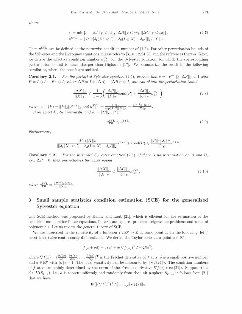
Diao H A et al. Sci China Math May 2013 Vol. 56 No. 5 973
where
ε := min{ε | ‖ΔA‖F � εδ1, ‖ΔB‖F � εδ2, ‖ΔC‖F � εδ3}, (2.7)
κSYL := ‖P−1[δ1(XT ⊗ I),−δ2(I ⊗X),−δ3I]‖2/‖X‖F .
Then κSYL can be defined as the normwise condition number of (1.2). For other perturbation bounds of
the Sylvester and the Lyapunov equations, please refer to [3,10–12,24,30] and the references therein. Next,
we derive the effective condition number κSYLEff for the Sylvester equation, for which the corresponding
perturbation bound is much sharper than Higham’s [17]. We summarize the result in the following
corollaries, where the proofs are omitted.
Corollary 2.1. For the perturbed Sylvester equation (2.5), assume that δ = ‖P−1‖2‖ΔP‖2 < 1 with
P = I ⊗A−BT ⊗ I, where ΔP = I ⊗ (ΔA)− (ΔB)T ⊗ I, one can obtain the perturbation bound
‖ΔX‖F‖X‖F � 1
1− δ
(‖ΔP‖2‖P‖2 cond(P ) +
‖ΔC‖F‖C‖F κSYL
Eff
), (2.8)
where cond(P ) = ‖P‖2‖P−1‖2 and κSYLEff := ‖C‖F
sep(A,B)‖X‖F= ‖P−1‖2‖C‖F
‖X‖F.
If we select δ1, δ2 arbitrarily, and δ3 = ‖C‖F , then
κSYLEff � κSYL. (2.9)
Furthermore,
‖P‖2‖X‖F‖[δ1(XT ⊗ I),−δ2(I ⊗X),−δ3I]‖2κ
SYL � cond(P ) � ‖P‖2‖X‖F‖C‖F κSYL.
Corollary 2.2. For the perturbed Sylvester equation (2.5), if there is no perturbation on A and B,
i.e., ΔP = 0, then one achieves the upper bound
‖ΔX‖F‖X‖F � ‖ΔC‖F
‖C‖F κSYLEff , (2.10)
where κSYLEff = ‖P−1‖2‖C‖F
‖X‖F.
3 Small sample statistics condition estimation (SCE) for the generalized
Sylvester equation
The SCE method was proposed by Kenny and Laub [21], which is efficient for the estimation of the
condition numbers for linear equations, linear least squares problems, eigenvalue problems and roots of
polynomials. Let us review the general theory of SCE.
We are interested in the sensitivity of a function f : Rp → R at some point x. In the following, let f
be at least twice continuously differentiable. We derive the Taylor series at a point x ∈ Rp,
f(x+ δd) = f(x) + δ(∇f(x))Td+O(δ2),
where ∇f(x) = (∂f(x)∂x1, ∂f(x)
∂x2, . . . , ∂f(x)∂xp
)T is the Frechet derivative of f at x, δ is a small positive number
and d ∈ Rp with ‖d‖2 = 1. The local sensitivity can be measured by ‖∇f(x)‖2. The condition numbers
of f at x are mainly determined by the norm of the Frechet derivative ∇f(x) (see [21]). Suppose that
d ∈ U(Sp−1), i.e., d is chosen uniformly and randomly from the unit p-sphere Sp−1, it follows from [21]
that we have
E(|(∇f(x))Td|) = ωp‖∇f(x)‖2,

974 Diao H A et al. Sci China Math May 2013 Vol. 56 No. 5
where E(·) is the expectation and ωp is the Wallis factor (cf. [21]) which only depends on p. The Wal-
lis factor
ωp =
⎧⎪⎪⎪⎪⎪⎪⎪⎪⎪⎨⎪⎪⎪⎪⎪⎪⎪⎪⎪⎩
1, for p = 1,2
π, for p = 2,
1 · 3 · 5 · · · (p− 2)
2 · 4 · 6 · · · (p− 1), for p odd and p > 2,
2
π
2 · 4 · 6 · · · (p− 2)
1 · 3 · 5 · · · (p− 1), for p even and p > 2,
can be accurately approximated by using a result in [21],
ωp ≈√
2
π(p− 12 )
. (3.1)
Therefore, we use ν = |(∇f(x))Td|/ωp as a condition estimator, which can estimate ‖∇f(x)‖2 with high
probability for the function f at x, i.e., for γ > 1 we have
Prob
(‖∇f(x)‖2γ
� ν � γ‖∇f(x)‖2)
� 1− 2
πγ+O
(1
γ2
).
To improve the accuracy of the condition estimator, we prefer more samples [21] in the following way.
Firstly, one can select d1, d2, . . . , dk ∈ U(Sp−1) and then use a QR decomposition [18] to produce an
orthonormal basis {d1, d2, . . . , dk}. Thus the orthogonal vectors d1, d2, . . . , dk ∈ Sp−1 span V which is
uniformly and randomly selected from the space of all k-dimensional subspaces of Rp. Then the expected
value of the norm of the projection of ∇f(x) onto V is given by [21]
E(√
|∇f(x)Td1|2 + |∇f(x)Td2|2 + · · ·+ |∇f(x)Tdk|2)=
ωp
ωk‖∇f(x)‖2,
where ωp and ωk are Wallis factors with orders p and k, respectively. A subspace condition estimator
ν(k) =ωk
ωp
√|∇f(x)Td1|2 + |∇f(x)Td2|2 + · · ·+ |∇f(x)Tdk|2
has the following probability for the estimator accuracy (cf. [21]):
Prob
(‖∇f(x)‖2γ
� ν(2) � γ‖∇f(x)‖2)
≈ 1− π
4γ2,
Prob
(‖∇f(x)‖2γ
� ν(3) � γ‖∇f(x)‖2)
≈ 1− 32
3π2γ3,
Prob
(‖∇f(x)‖2γ
� ν(4) � γ‖∇f(x)‖2)
≈ 1− 81π2
512γ4.
For example, if we take k = 3 and γ = 10, then the estimator ν(3) has probability 1 − 323π2103 ≈ 0.9989
with a relative factor of 10 of the true condition number ‖∇f(x)‖2.Now we apply SCE to estimate the normwise, mixed and componentwise condition numbers for (1.1)
in the following two sub-sections. We firstly derive the directional derivative of (1.1) at the input data
(A,B,C,D,E, F ) with respect to the direction (A,B, C,D, E ,F). Suppose that [X + δX , Y + δY] is theexact solution of {
(A+ δA)(X + δX )− (Y + δY)(B + δB) = C + δC,(D + δD)(X + δX )− (Y + δY)(E + δE) = F + δF ,
where δ ∈ R. Consider the difference of the above equations and (1.1), divided by δ. When δ → 0, we
conclude that {AX − YB = C − AX + Y B,DX − YE = F −DX + Y E . (3.2)

Diao H A et al. Sci China Math May 2013 Vol. 56 No. 5 975
The solution to (3.2) is the directional derivative of (1.1) at the input data (A,B,C,D,E, F ) with respect
to the direction (A,B, C,D, E ,F).
Remark 1. When we solve the generalized Sylverster equation (1.1) by means of the generalized
Schur decomposition [20], if the decompositions (1.4) of A,B,D and E are obtained, then (3.2) can be
solved efficiently.
3.1 Normwise perturbation analysis
By means of SCE, we devise the algorithms for the normwise condition estimation of (1.1). We introduce
the ‘unvec’ operation: for v = (v1, v2, . . . , vn2) ∈ R1×n2
, then A = unvec(v) sets the entries of A to
aij = vi+(j−1)n.
Algorithm 3.1 (One sample condition estimation for the solution [X,Y ] to the generalized Sylvester
equation (1.1)). 1. Let A, D ∈ Rm×m, B, E ∈ R
n×n and C, F ∈ Rm×n be selected randomly and
independently from a normal distribution with mean 0 and variance 1, i.e., each entry is in N (0, 1).
Denote η = ‖(A,B, C,D, E ,F)‖F and set A = A/η, B = B/η, C = C/η, D = D/η, E = E/η and F = F/η.
2. Let p = 2(m2 + n2 +mn). Approximate ωp by (3.1).
3. Solve the generalized Sylvester equation (3.2).
4. Calculate the condition number based on the small sample estimation,
KGSYLabs =
1
ωp|[X ,Y]|, nGSYL
F,SCE =1
ωp‖[X ,Y]‖F = ‖KGSYL
abs ‖F ,
where |[X ,Y]| is a matrix whose entries are the absolute values of the corresponding entries of [X ,Y].Define the relative condition number κGSYL
F,SCE = nGSYLF,SCE/‖[X,Y ]‖F .
Algorithm 3.2 (Subspace condition estimation for the solution [X,Y ] to the generalized Sylvester equa-
tion (1.1)). 1. Generate matrices (A1,B1, C1,D1, E1,F1), (A2,B2, C2,D2, E2,F2), . . . , (Ak,Bk, Ck,Dk,
Ek,Fk) with entry being in N (0, 1). With the QR factorization of⎡⎢⎢⎢⎢⎢⎣vec(A1) vec(A2) · · · vec(Ak)
vec(B1) vec(B2) · · · vec(Bk)
· · · · · · . . . · · ·vec(F1) vec(F2) · · · vec(Fk)
⎤⎥⎥⎥⎥⎥⎦form an orthonormal matrix [q1, q2, . . . , qk]. Each qi can be converted into the desired matrices (Ai,Bi, Ci,Di, Ei,Fi) with the unvec operation.
2. Let p = 2(m2 + n2 +mn). Approximate ωp and ωk by (3.1).
3. Solve the generalized Sylvester equations (3.2) with the matrix (Ai,Bi, Ci,Di, Ei,Fi), i = 1, 2, . . . , k.
4. Compute the condition number
nGSYL,(k)F,SCE :=
ωk
ωp
√‖[X1,Y1]‖2F + ‖[X2,Y2]‖2F + · · ·+ ‖[Xk,Yk]‖2F = ‖KGSYL,(k)
abs ‖F ,
KGSYL,(k)abs :=
ωk
ωp
√|[X1,Y1]|2 + |[X2,Y2]|2 + · · ·+ |[Xk,Yk]|2,
where the square root and the power operation of the second equation are applied at each entry of
[Xi,Yi], i = 1, 2, . . . , k. Note that every operation run in the second equation is meant to be performed
componentwise, and not in the sense of matrices.
Define the normwise condition number: κGSYL,(k)F,SCE = n
GSYL,(k)F,SCE /‖[X,Y ]‖F .
In Step 1 of Algorithm 3.2, if we use the Householder transformation [18] to compute the QR decompo-
sition to form an orthonormal matrix [q1, q2, . . . , qk], then we need 8k2(m2+n2+mn)− 43k
2 flops. To form
the right-hand side of (3.2), the total cost is 4m2n+ 4mn2 − 2mn flops. If we use the generalized Schur
decomposition [20] to solve (1.1), then A and B are upper quasi-triangular, and D, E are upper triangular
matrices. The total flops of solving (3.2) with A,B,D and E in standard form is 5m2n+ 5mn2 + 974 mn

976 Diao H A et al. Sci China Math May 2013 Vol. 56 No. 5
at most according to [20]. Then the third step of Algorithm 3.2 needs 9m2n + 9mn2 + 894 mn flops
at most. The last step of Algorithm 3.2 uses 4kmn flops. At end the total cost of Algorithm 3.2 is
9m2n+ 9mn2 + (894 + 8k2 + 4k)mn+ 8k2(m2 + n2)− 43k
2 flops, which is lower compared with the total
cost O(m3 + n3) flops of the generalized Schur decomposition [20] to solve (1.1). Generally with k = 3,
the algorithm yields accurate estimates of condition numbers efficiently.
Remark 2. SCE method can be used to estimate the effective condition number κGSYLEff . Recall
that κGSYLEff = ‖Z−1‖2‖[C,F ]‖F
‖[X,Y ]‖F, the main task is to estimate ‖Z−1‖2. From the theory of SCE [21], we
can generate the orthogonal vectors l1, l2, . . . , lk ∈ Sp−1 uniformly and randomly with p = 2mn by
QR factorization. Firstly we calculate Z−1li, while Z−1li is the solution to a generalized Sylvester
equation (1.3). As pointed in Remark 1, Z−1li can be computed efficiently when we have the generalized
Schur decomposition [20]. Finally ‖Z−1‖2 can be estimated by
ωk
ωp‖√|Z−1l1|2 + |Z−1l2|2 + · · ·+ |Z−1lk|2‖2
with high probability.
3.2 Componentwise perturbation analysis
In componentwise perturbation analysis, for a perturbation Δa on a ∈ R, it should satisfy |Δa| � εa.
For a perturbation ΔA = (Δaij) on a matrix A = (aij) ∈ Rm×n, it is a componentwise perturbation, if
|ΔA| � ε|A| or |Δaij | � ε|aij |.
We can write ΔA = δ(A�A) with |δ| � ε and each entries of A being in the interval [−1, 1], where � is
a Hadamard product (cf. [26]). Based on the above observation, we obtain a componentwise sensitivity
of (1.1)’s solution [X,Y ] in the following manner. We can modify Algorithm 3.2 directly, i.e., after
generating and normalizing (or orthonormalizing as in Algorithm 3.2) the random elements of Step 1, these
elements are multiplied by the corresponding entries of A,B,C,D,E or F , respectively. The remaining
steps of the algorithm are unchanged. In the following, let ‖A‖max = ‖vec(A)‖∞ and AB = (
aij
bij) with A =
(aij) and B = (bij). Assume [Xi,Yi] is the solution to (3.2) with the random matrix (Ai,Bi, Ci,Di, Ei,Fi)
as in Algorithm 3.2, whereas (Ai,Bi, Ci,Di, Ei,Fi) are obtained by multiplying (Ai,Bi, Ci,Di, Ei,Fi) with
the associated entries of A,B,C,D,E or F , respectively, in the first step of Algorithm 3.2. Let us denote
the mixed condition number mGSYL,(k) and componentwise condition number cGSYL,(k) as follows:
mGSYL,(k) := ‖MGSYL,(k)‖max/‖[X,Y ]‖max, cGSYL,(k) :=
∥∥∥∥MGSYL,(k)
[X,Y ]
∥∥∥∥max
, (3.3)
where MGSYL,(k) = ωk
ωp
√|[X1,Y1]|2 + |[X2,Y2]|2 + · · ·+ |[Xk,Yk]|2.Remark 3. Since the algorithm of the estimation for mGSYL,(k) and cGSYL,(k) is only different in the
first step of Algorithm 3.2, an extra 2k(m2 + n2 + mn) flops for matrix componentwise multiplication
will be needed. Then the total flop count to estimate mGSYL,(k) and cGSYL,(k) is 9m2n + 9mn2 + (894+ 8k2 + 6k)mn+ (8k2 + 2k)(m2 + n2)− 4
3k2 at most.
4 Numerical examples
In this section, we present some examples to show the sharpness of our perturbation bounds. All numerical
examples are carried out by Matlab 7.0, with machine epsilon ε ≈ 2.2 × 10⁻¹⁶. Here we choose δ1 =
‖A‖F , δ2 = ‖B‖F , δ3 = ‖C‖F , δ4 = ‖D‖F , δ5 = ‖E‖F and δ6 = ‖F‖F to compute κSYL and κGSYL
in (1.7) and (2.7), respectively.
To illustrate the differences between the effective condition number κGSYLEff and the normwise condition
number κGSYL for the generalized Sylvester equation in Theorem 2.1, we test several numerical examples.
From the given examples, we see that the effective condition number captures the conditioning of the

Diao H A et al. Sci China Math May 2013 Vol. 56 No. 5 977
problem well, if there are only perturbations on the right-hand sides [C,F ], without perturbations on
A,B,D, and E in (1.1), i.e., ΔZ = 0 in (2.1) of Theorem 2.1. We add some random perturbations on
the right-hand sides [C,F ] and compare the actual perturbation error ‖[ΔX,ΔY ]‖F
‖[X,Y ]‖Fwith the first order
perturbation bound given by the effective condition number
‖[ΔC,ΔF ]‖F‖[C,F ]‖F κGSYL
Eff .
From the numerical examples, the effective condition number κGSYLEff gives sharper perturbation bounds.
Example 4.1 (See [40]). Consider the real regular matrix pair (A,B) with
A = V
[A −C
0 B
]UT, B = V
[D −F
0 E
]UT,
where U and V are orthogonal matrices with
A =
⎡⎢⎢⎣1 0 0
0 −5 0
0 0 10−k
⎤⎥⎥⎦ , B =
⎡⎢⎢⎣10k 0 0
0 2 0
0 0 −10−l
⎤⎥⎥⎦ , C = −
⎡⎢⎢⎣2× 10k 1 0
0 −1 3
0 0 0
⎤⎥⎥⎦ ,
and
D =
⎡⎢⎢⎣−4× 10−k 0 0
0 3 0
0 0 −2× 10−l
⎤⎥⎥⎦ , E =
⎡⎢⎢⎣1 0 0
0 1 0
0 0 −10−k
⎤⎥⎥⎦ , F = −
⎡⎢⎢⎣7 2 0
0 5 1
0 0 −3× 10k
⎤⎥⎥⎦ .
In order to compute the eigenpair of the matrix pair (A,B), we need to solve the generalized Sylvester
equation (1.1).
In the following, we test different choices k and l to show that κGSYLEff is much smaller than κGSYL. From
Table 1, we find when k = l, κGSYL ≈ 10k+l, but κGSYLEff is always O(1). Let randn(m,n) denote an m×n
random perturbation matrix with each entry in N (0, 1). We generate some random perturbations on the
right-hand side C and F , where ΔC = ε · randn(m,n),ΔF = ε · randn(m,n) for different perturbation
parameters ε, then we compare the first order perturbation bound ‖[ΔC,ΔF ]‖F
‖[C,F ]‖FκGSYLEff given by the effec-
tive condition number with the actual error bound ‖[ΔX,ΔY ]‖F
‖[X,Y ]‖F. From the first to third columns, we see
that ‖[ΔX,ΔY ]‖F
‖[X,Y ]‖Fhas the same order of ‖[ΔC,ΔF ]‖F
‖[C,F ]‖FκGSYLEff , which indicates that κGSYL
Eff gives tighter error
bounds than κGSYL. For the fourth column, the perturbation bound by the effective condition number
is much larger than the true relative error, however we can trust the computational solution since the
problem is well-conditioned in the setting of the effective condition number. Even for the ill-conditioned
case k = 10, l = 1, the bound ‖[ΔC,ΔF ]‖F
‖[C,F ]‖FκGSYLEff is only 10 times that of the true error. For the last
column, in the normwise perturbation sense, the problem is very ill-conditioned as the normwise condi-
tion number κGSYL has the order of 20. If there are only perturbations on the right-hand sides, then we
Table 1 The comparison of κGSYL, κGSYLEff ,
‖[ΔC,ΔF ]‖F‖[C,F ]‖F κGSYL
Eff and‖[ΔX,ΔY ]‖F
‖[X,Y ]‖F
k = l = 2 k = 2, l = 5 k = l = 5 k = 10, l = 1 k = l = 10
κGSYL 1.5838e+004 1.4435e+004 1.5811e+010 5.0360e+010 1.5811e+020
κGSYLEff 2.4782 100.1887 2.5039e+003 4.0172e+009 2.4777
‖[ΔC,ΔF ]‖F‖[C,F ]‖F 1.8894e−011 9.9243e−012 1.0601e−014 8.0632e−020 1.2198e−019
‖[ΔX,ΔY ]‖F‖[X,Y ]‖F 2.3971e−011 1.7072e−010 1.0314e−014 7.5077e−011 5.3479e−020

978 Diao H A et al. Sci China Math May 2013 Vol. 56 No. 5
compute the solution accurately, and the effective condition number κGSYLEff reveals the true conditioning of
the problem.
Next, we will test four numerical examples of the Sylvester equations from [8,41–43] to demonstrate the
effective condition number κSYLEff in Corollary 2.1 are much smaller than Higham’s normwise condition
number κSYL in (2.7). Also we add some random perturbations on the right-hand matrix C in the
standard Sylvester equation AX −XB = C with ΔC = ε · randn(m,n). We compare the true relative
errors ‖ΔX‖F
‖X‖Fwith the first order perturbation bound given by the effective condition number ‖ΔC‖F
‖C‖FκSYLEff .
The numerical examples show that ‖ΔC‖F
‖C‖FκSYLEff gives sharper perturbation bounds.
Example 4.2 (See [8, p. 267]). This example is from the discretization of the two-dimensional Poisson
equation as in Section 1, the coefficient matrices A,B ∈ Rn×n in the Sylvester equation AX −XB = C
have the tridiagonal structure as follows,
A = −B =
⎡⎢⎢⎢⎢⎢⎢⎣2 −1 0
−1. . .
. . .
. . .. . . −1
0 −1 2
⎤⎥⎥⎥⎥⎥⎥⎦ .
We choose C = (cij) = h2 exp (ih+ jh), i, j = 1, 2, . . . , n, where h = 1n+1 is the discretization step size.
Next we compare κSYL, κSYLEff , ‖ΔC‖F
‖C‖FκSYLEff and ‖ΔX‖F
‖X‖Ffor different choices of n (see Table 2).
Example 4.3 (See [41, 42]). The matrix in this example presents a Hamiltonian-like structure,
H = QT
[A −C
0 −AT
]Q, A =
⎡⎢⎢⎢⎢⎣1− α α
α 1− α
α 1− α
α 1− α
⎤⎥⎥⎥⎥⎦ ∈ R4×4,
where C = randn(4, 4), and Q is a random orthogonal matrix. In order to compute the eigenpair of the
matrix H , we need to solve the Sylvester equation
AX −XB = C, B = −AT. (4.1)
Next we compare κSYL, κSYLEff , ‖ΔC‖F
‖C‖FκSYLEff and ‖ΔX‖F
‖X‖Ffor different choices of α. It is shown that when
α approximates to 1/2, κSYL increases more, while κSYLEff changes a little bit (see Table 3).
Example 4.4 (See [43]). Let m = n, C = randn(m,n), and A = −B = I − wUn − θeneT1 , where
Un =
⎡⎢⎢⎢⎢⎢⎢⎣0 1
0. . .
. . . 1
0
⎤⎥⎥⎥⎥⎥⎥⎦Table 2 The comparison of κSYL, κSYL
Eff , ‖ΔC‖F‖C‖F κSYL
Eff and ‖ΔX‖F‖X‖F
n = 5 n = 10 n = 20 n = 50
κSYL 13.9146 65.9868 341.2454 3.1933e+003
κSYLEff 1.1338 1.2209 1.2824 1.3272
‖ΔC‖F‖C‖F 3.6812e−010 3.1934e−010 3.0396e−010 3.2062e−010
‖ΔX‖F‖X‖F 8.3033e−011 3.6238e−011 2.1271e−011 1.1388e−011
Diao H A et al. Sci China Math May 2013 Vol. 56 No. 5 979
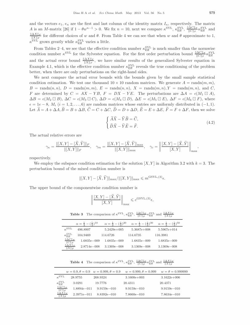
and the vectors e1, en are the first and last column of the identity matrix In, respectively. The matrix
A is an M -matrix [26] if 1 − θwn−1 > 0. We fix n = 10, next we compare κSYL, κSYLEff , ‖ΔC‖F
‖C‖FκSYLEff and
‖ΔX‖F
‖X‖Ffor different choices of w and θ. From Table 4 we can see that when w and θ approximate to 1,
κSYL grows greatly while κSYLEff varies a little.
From Tables 2–4, we see that the effective condition number κSYLEff is much smaller than the normwise
condition number κSYL for the Sylvester equation. For the first order perturbation bound ‖ΔC‖F
‖C‖FκSYLEff
and the actual error bound ‖ΔX‖F
‖X‖F, we have similar results of the generalized Sylvester equation in
Example 4.1, which is the effective condition number κSYLEff reveals the true conditioning of the problem
better, when there are only perturbations on the right-hand sides.
We next compare the actual error bounds with the bounds given by the small sample statistical
condition estimation. We test one thousand 10 × 10 random matrices. We generate A = randn(m,m),
B = randn(n, n), D = randn(m,m), E = randn(n, n), X = randn(m,n), Y = randn(m,n), and C,
F are determined by C = AX − Y B, F = DX − Y E. The perturbations are ΔA = ε(M1 � A),
ΔB = ε(M2 � B), ΔC = ε(M3 � C), ΔD = ε(M4 � D), ΔE = ε(M5 � E), ΔF = ε(M6 � F ), where
ε = 1e − 8, Mi (i = 1, 2, . . . , 6) are random matrices whose entries are uniformly distributed in (−1, 1).
Let A = A+ΔA, B = B +ΔB, C = C +ΔC, D = D+ΔD, E = E +ΔE, F = F +ΔF , then we solve{AX − Y B = C,
DX − Y E = F .(4.2)
The actual relative errors are
γκ =‖[X,Y ]− [X, Y ]‖F
‖[X,Y ]‖F , γm =‖[X,Y ]− [X, Y ]|max
‖[X,Y ]‖max, γc =
∥∥∥∥ [X,Y ]− [X, Y ]
[X,Y ]
∥∥∥∥max
,
respectively.
We employ the subspace condition estimation for the solution [X,Y ] in Algorithm 3.2 with k = 3. The
perturbation bound of the mixed condition number is
‖[X,Y ]− [X, Y ]‖max/‖[X,Y ]‖max � mGSYL,(3)ε.
The upper bound of the componentwise condition number is∥∥∥∥ [X,Y ]− [X, Y ]
[X,Y ]
∥∥∥∥max
� cGSYL,(3)ε,
Table 3 The comparison of κSYL, κSYLEff , ‖ΔC‖F
‖C‖F κSYLEff and ‖ΔX‖F
‖X‖F
α = 12− ( 1
2)10 α = 1
2− ( 1
2)20 α = 1
2− ( 1
2)30 α = 1
2− ( 1
2)50
κSYL 496.8907 5.2429e+005 5.3687e+008 5.5967e+014
κSYLEff 104.9469 114.6726 114.6735 116.3981
‖ΔC‖F‖C‖F 1.6835e−009 1.6835e−009 1.6835e−009 1.6835e−009
‖ΔX‖F‖X‖F 2.8714e−008 3.1369e−008 3.1369e−008 3.1369e−008
Table 4 The comparison of κSYL, κSYLEff , ‖ΔC‖F
‖C‖F κSYLEff and ‖ΔX‖F
‖X‖F
w = 0.9, θ = 0.9 w = 0.999, θ = 0.9 w = 0.999, θ = 0.999 w = θ = 0.999999
κSYL 28.9755 268.9324 3.1600e+003 3.1622e+006
κSYLEff 3.0291 19.7776 20.4311 20.4371
‖ΔC‖F‖C‖F 1.8894e−011 9.9159e−010 9.9159e−010 9.9159e−010
‖ΔX‖F‖X‖F 2.3971e−011 8.8392e−010 7.8660e−010 7.8634e−010

980 Diao H A et al. Sci China Math May 2013 Vol. 56 No. 5
where mGSYL,(3) and cGSYL,(3) are given by (3.3) with k = 3. Recall that κGSYL,(3)F,SCE is defined in
Algorithm 3.2 with k = 3. The perturbation bound of the normwise condition number is
‖[X,Y ]− [X, Y ]‖F /‖[X,Y ]‖F � κGSYL,(3)F,SCE ε.
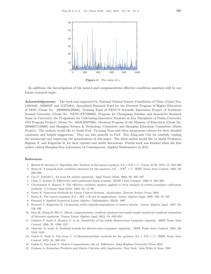
We denote three overestimate ratios as follows:
rn :=κGSYL,(3)F,SCE
γκε, rm :=
mGSYL,(3)
γmε, rc :=
cGSYL,(3)
γcε.
These ratios demonstrate the efficiency of small sample statistical condition estimations. The ratios
are displayed in Figures 1–3. Among 1000 tests, the ratios in most cases are of order 1, except a few
exceptional cases. The average values of rn, rm and rc are 1.6927, 2.4087 and 2.8434, respectively.
Usually an estimate of the condition number that is correct to within a factor 10 is acceptable, see [18,
Chapter 15] for details. We see that the small sample statistical method is quite effective for condition
number estimation. It also yields tighter error bounds on average.
5 Concluding remarks
We apply the concept of effective condition numbers to the Sylvester and the generalized Sylvester equa-
tions. Sharper perturbation bounds based on the effective condition numbers are obtained. From the
numerical tests, the effective condition numbers are much smaller than the normwise condition numbers.
The small sample statistical condition estimation algorithms for the normwise, mixed and componentwise
condition numbers of the generalized Sylvester equation are also proposed, which are very effective for
the numerical examples.
30
25
20
15
10
5
00 200 400 600 800 1000
Figure 1 The value of rn
0 200 400 600 800 1000
70
60
50
40
30
20
10
0
Figure 2 The value of rm
Diao H A et al. Sci China Math May 2013 Vol. 56 No. 5 981
0 200 400 600 800 1000
60
50
40
30
20
10
0
Figure 3 The value of rc
In addition, the investigation of the mixed and componentwise effective condition numbers will be our
future research topic.
Acknowledgements The work was supported by National Natural Science Foundation of China (Grant Nos.
11001045, 10926107 and 11271084), Specialized Research Fund for the Doctoral Program of Higher Education
of MOE (Grant No. 20090043120008), Training Fund of NENU’S Scientific Innovation Project of Northeast
Normal University (Grant No. NENU-STC08009), Program for Changjiang Scholars and Innovative Research
Team in University, the Programme for Cultivating Innovative Students in Key Disciplines of Fudan University
(973 Program Project) (Grant No. 2010CB327900), Doctoral Program of the Ministry of Education (Grant No.
20090071110003) and Shanghai Science & Technology Committee and Shanghai Education Committee (Dawn
Project). The authors would like to thank Prof. Ya-xiang Yuan and three anonymous referees for their detailed
comments and helpful suggestions. They are also grateful to Prof. Eric King-wah Chu for carefully reading
the manuscript and improving the presentations of this paper. The third author would like to thank Professors
Higham N. and Kagstrom B. for their reprints and useful discussions. Partial work was finished when the first
author visited Shanghai Key Laboratory of Contemporary Applied Mathematics in 2012.
References
1 Bartels R, Stewart G. Algorithm 432: Solution of the matrix equation AX+XB = C. Comm ACM, 1972, 15: 820–826
2 Byers R. A Linpack-style condition estimator for the equation AX −XBT = C. IEEE Trans Auto Control, 1984, 29:
926–928
3 Cao Y, Petzold L. An error for matrix equations. Appl Numer Math, 2004, 50: 395–407
4 Chan T, Foulser D. Effectively well-conditioned linear systems. SIAM J Stat Comput, 1988, 9: 963–969
5 Christiansen S, Hansen P. The effective condition number applied to error analysis of certain boundary collocation
methods. J Comput Appl Math, 1994, 54: 15–36
6 Datta B. Numerical Methods for Linear Control Systems. Amsterdam: Elsevier Science Press, 2004
7 Datta K. The matrix equation XA− BX = R and its applications. Linear Algebra Appl, 1988, 109: 91–105
8 Demmel J. Applied Numerical Linear Algebra. Philadelphia: SIAM, 1997
9 Demmel J, Kagstrom B. Computing stable eigendecompositions of matrix pencils. Linear Algebra Appl, 1987, 88:
139–186
10 Diao H, Xiang H, Wei Y. Mixed, componentwise condition numbers and small sample statistical condition estimation
of Sylvester equations. Numer Linear Algebra Appl, 2012, 19: 639–654
11 Gahinet P, Laub A, Kenney C, et al. Sensitivity of the stable discrete-time Lyapunov equation. IEEE Trans Auto
Control, 1990, 35: 1209–1217
12 Ghavimi A, Laub A. Residual bounds for discrete-time Lyapunov equations. IEEE Trans Auto Control, 1995, 40:
1244–1249
13 Golub G, Nash S, Van Loan C. A Hessenberg-Schur methods for the problem AX + XB = C. IEEE Trans Auto
Control, 1979, 24: 909–913
14 Golub G, Van Loan C. Matrix Computations, 4th ed. Baltimore: John Hopkins University Press, 2013
15 Graham A. Kronecker Products and Matrix Calculus with Application. New York: John Wiley & Sons, 1981
982 Diao H A et al. Sci China Math May 2013 Vol. 56 No. 5
16 Hearon J. Nonsingular solution of TA−BT = C. Linear Algebra Appl, 1977, 16: 57–63
17 Higham N. Perturbation theory and backward error for AX −XB = C. BIT, 1993, 33: 124–136
18 Higham N. Accuracy and Stability of Numerical Algorithms, 2nd ed. Philadelphia: SIAM, 2002
19 Kagstrom B. A perturbation analysis of the generalized Sylvester equation (AR − LB,DR − LE) = (C, F ). SIAM J
Matrix Anal Appl, 1994, 15: 1045–1060
20 Kagstrom B, Westin L. Generalized Schur methods with estimators for solving the generalized Sylvester equation.
IEEE Trans Auto Control, 1989, 34: 745–751
21 Kenney C, Laub A. Small-sample statistical condition estimates for general matrix functions. SIAM J Sci Comput,
1994, 15: 36–61
22 Kenney C, Laub A, Reese M. Statistical condition estimation for the linear least squares. SIAM J Matrix Anal Appl,
1998, 19: 906–923
23 Konstantinov M, Gu D, Mehrmann V, et al. Perturbation Theory for Matrix Equations. Amsterdam: Elsevier Science
Press, 2003
24 Konstantinov M, Petkov P, Gu D, et al. Sensitivity of General Lyapunov Equations. Leicester: Leicester University
Press, 1993
25 Lancaster P. Explicit solution of linear matrix equations. SIAM Rev, 1970, 12: 544–566
26 Lancaster P, Tismenetsky M. The Theory of Matrices, 2nd ed. Orlando, FL: Academic Press, 1985
27 Laub A, Xia J. Applications of statistical condition estimation to the solution of linear systems. Numer Linear Algebra
Appl, 2008, 15: 489–513
28 Laub A, Xia J. Statistical condition estimation for the roots of polynomials. SIAM J Sci Comput, 2008, 31: 624–643
29 Laub A, Xia J. Fast condition estimation for a class of structured eigenvalue problems. SIAM J Matrix Anal Appl,
2009, 30: 1658–1676
30 Lesecq S, Barraud A, Christov N. On the local sensitivity of the Lyapunov equations. In: Vulkov L, Wasniewski J,
Yalamov P, eds. Numerical Analysis and Its Applications. Berlin: Springer, 2001, 521–526
31 Li Z, Chien C, Huang H. Effective condition number for finite difference method. J Comput Appl Math, 2007, 198:
208–235
32 Li Z, Huang H. Effective condition number for numerical partial diffrential equations. Numer Linear Algebra Appl,
2008, 15: 575–594
33 Li Z, Huang H, Chen J, et al. Effective condition number and its application. Computing, 2010, 89: 87–112
34 Li Z, Huang H, Wei Y, et al. Effective Condition Number for Numerical Partial Differential Equations. Beijing: Science
Press, 2013
35 Lin Y, Wei Y. Condition numbers of the generalized Sylvester equation. IEEE Trans Auto Control, 2007, 53: 2380–2385
36 Rice J. A theory of condition. SIAM J Numer Anal, 1966, 3: 217–232
37 Rice J. Matrix Computations and Mathematical Software. New York: McGraw-Hill Book Company, 1981
38 Stewart G. Error and perturbation bounds for subspaces associated with certain eigenvalue problems. SIAM Rev,
1973, 15: 727–764
39 Stewart G, Sun J. Matrix Perturbation Theory. New York: Academic Press, 1990
40 Sun J. Condition Numbers of the Spectral Projections. Sweden: Umea University Press, 2002
41 Sun X, Quintana-Ortı E. The generalized Newton iteration for the matrix sign function. SIAM J Sci Comput, 2002,
24: 669–683
42 Sun X, Quintana-Ortı E. Spectral division methods for block generalized Schur decompositions. Math Comput, 2004,
73: 1827–1847
43 Xue J, Xu S, Li R. Accurate solutions of M -matrix Sylvester equations. Numer Math, 2012, 120: 639–670