Effective Community Search over Large Spatial Graphs

Yixiang Fang, Reynold Cheng, Xiaodong Li, Siqiang Luo, Jiafeng HuDepartment of Computer Science, The University of Hong Kong, Hong Kong

{yxfang, ckcheng, xdli, sqluo, jhu}@cs.hku.hk

ABSTRACTCommunities are prevalent in social networks, knowledge graphs,and biological networks. Recently, the topic of community search(CS) has received plenty of attention. Given a query vertex, CSlooks for a dense subgraph that contains it. Existing CS solutionsdo not consider the spatial extent of a community. They canyield communities whose locations of vertices span large areas. Inapplications that facilitate the creation of social events (e.g., findingconference attendees to join a dinner), it is important to find groupsof people who are physically close to each other. In this situation,it is desirable to have a spatial-aware community (or SAC), whosevertices are close structurally and spatially. Given a graph G and aquery vertex q, we develop exact solutions for finding an SAC thatcontains q. Since these solutions cannot scale to large datasets, wehave further designed three approximation algorithms to computean SAC. We have performed an experimental evaluation for thesesolutions on both large real and synthetic datasets. Experimentalresults show that SAC is better than the communities returned byexisting solutions. Moreover, our approximation solutions can findSACs accurately and efficiently.

1. INTRODUCTIONWith the emergence of geo-social networks, such as Twitter

and Foursquare, the topic of geo-social networks has gained alot of attention [1, 30, 26, 12]. In these networks, a user isoften associated with location information (e.g., positions of herhometown and check-ins). These networks are collectively knownas spatial graphs. Figure 1 depicts a spatial graph with nine usersin three cities Berlin, Paris, London, and each user has aspecific location. The solid lines represent their social relationship,and the dashed lines denote their hometown locations.

In this paper, we study the problem of performing onlinecommunity search (CS) on spatial graphs. Given a spatial graphG and a vertex q ∈ G, our goal is to find a subgraph of G, calleda spatial-aware community (or SAC). Essentially, a community isa social unit of any size that shares common values, or that issituated in a close area [22]. An SAC is such a community withhigh structure cohesiveness and spatial cohesiveness. The structure

This work is licensed under the Creative Commons Attribution-NonCommercial-NoDerivatives 4.0 International License. To view a copyof this license, visit http://creativecommons.org/licenses/by-nc-nd/4.0/. Forany use beyond those covered by this license, obtain permission by emailinginfo@vldb.org.Proceedings of the VLDB Endowment, Vol. 10, No. 6Copyright 2017 VLDB Endowment 2150-8097/17/02.

Jack

Bob

Tom Jim

Jason

JohnEric

Leo

City1 City2 City3

Jeff

Jack

Bob

Tom Jim

Jason

JohnEric

Leo

Berlin Paris London

Jeff

Figure 1: A geo-social network.

cohesiveness mainly measures the social connections within thecommunity, while the spatial cohesiveness focuses on the closenessamong their geo-locations. Figure 1 illustrates an SAC with threeusers {Tom, Jeff, Jim}, in which each user is linked with eachother and all of them are in Paris.

Table 1: Works on community retrieval.GraphType

CommunityDetection (CD)

CommunitySearch (CS)

Non-spatial [25, 14] [29, 7, 6, 21, 19, 11]Spatial [16, 10, 4] SAC search

Prior works. The community retrieval methods can generallybe classified into community detection (CD) and communitysearch (CS), as shown in Table 1. Earlier CD methods [25,14] mainly focus on link analysis without considering spatialfeatures. Some recent studies [2] have shown that, in networkswhere vertices occupy positions in an Euclidian space, spatialconstraints may have a strong effect on their relationship patterns,so some works [16, 10, 4] have considered the spatial featuresfor community detection. All these CD methods often detectall the communities from an entire graph using some predefinedglobal criteria (e.g., modularity [20]), so their focus is beyondpersonalized community search. Also, their efficiency isinadequate for fast and online community retrieval since theyrequire to enumerate all the communities. To address theselimitations, some works [29, 7, 6, 19, 11] focus on onlinecommunity search, a query-dependent variant of communitydetection, and they are able to find communities for a specificvertex. However, almost all these CS works focus on link analysisand do not consider the spatial features. In Figure 1, for example,previous CS methods [29, 7] tend to put Jason and Tom, Jeff,Jim into the same community, although Jason is located inanother city London. This community may not be very useful

709

2016/6/9 Circles

file:///C:/Users/Admin/Dropbox/SAC%20search/workspace/sac/info/1064.html 1/1

B

A

Map data ©2016 Google

(a) user1’s SACs (b) user2’s SACs

Figure 2: SACs in Brightkite dataset.

for some location-based services (e.g., setting up events). Toalleviate this issue, in this paper we study SAC search whichfinds communities for a particular query vertex in an “online”manner. Our later experimental results on real datasets show that,the communities found by our methods are often in a much smallerareas than that of previous CS methods, i.e., the radii of the spatialcircles covering communities found by [29] and [7] are 50 and 20times larger than those of SAC search.

SAC search. We now discuss how to measure the structurecohesiveness and spatial cohesiveness of an SAC. We adopt thecommonly used metric minimum degree [29, 7, 21] to measure thestructure cohesiveness. Note that in our method, the minimumdegree metric can be easily replaced by other metrics likek-truss [19] and k-clique [6]. To measure the spatial cohesiveness,we consider the spatial circle, which contains all the communitymembers. In particular, given a query vertex q ∈ G, our goal is tofind an SAC containing q in the smallest minimum covering circle(or MCC) and all the vertices of the SAC satisfy the minimumdegree metric. The main features of SAC search are summarizedas follows.• Adaptability to location changes. In geo-social networks(e.g., Brightkite and Foursquare), a user’s location often changesfrequently, due to its nature of mobility. As a result, users’spatially close communities change frequently as well. Let usconsider two real examples in Brightkite, which once was a popularlocation-based social networking website. Figure 2(a) shows auser’s two SACs in two consecutive days, when she moves fromplace “A” to place “B” in US, in which each SAC is located in anMCC denoted by a circle. Note that all the members are differentexcept the user itself. Figure 2(b) shows another user’s two SACsin three days, when she moves from place “C” to place “D”. Thesereal examples clearly show that a user’s communities could evolveover time. In our later experiments, we find that for two SACs withtime gap of six hours or more, the average Jaccard similarity ofthese two community member sets decreases by 25%.

Moreover, the link relationship also evolves over time. Sothe existing CD methods may easily lose the freshness andeffectiveness after a short period of time. On the contrary, our SACsearch can adapt to such dynamic easily, as it can answer queries inan “online” manner. Also, our methods do not rely on any offlinecomputation, such as graph clustering or index structures.• Personalization. SAC search allows a query user to finda community that exhibits both high structure cohesiveness andspatial cohesiveness. The parameter k, the minimum degree,allows the user to control the strength of link intensiveness. Forexample, SAC search can answer queries such as who are my

nearby friends so that we can form a particular club? In contrast,existing CD methods [16, 10, 4] often use some global criteria (e.g.,modularity), and consider the static community detection problem,where the graph is partitioned a-priori with no reference to theparticular query vertices.• Online search. Similar to other online CS methods, ourmethod is able to find an SAC from a large spatial graph quicklyonce a query request arrives. However, existing CD methods forspatial graphs, are generally slower, as they are often designed forgenerating all the communities for an entire graph.

Applications. We now discuss the applications of SAC search.• Event recommendation. Emerging geo-social applications suchas Meetup1, Meetin2, and Eventbrite3 allow social network usersto meet physically for various interesting purposes (e.g., party,dinner, and dating). For example, Meetup tracks its users’ mobilephone locations, and suggests interesting location-based events tothem [30]. Suppose that Meetup wishes to recommend an eventto a user u. Then we can first find u’s SAC, whose membersare physically close to u. Events proposed by u’s SAC memberv can then be introduced to u, so that u can meet v if she isinterested in v’s activity. Since u’s location changes constantly,u’s recommendation needs to be updated accordingly. Also, theseapplications often have to handle requests from a large numberof online users efficiently. Our high-performance SAC searchalgorithms can therefore benefit these applications.• Social marketing. As studied in [23], people with close socialrelationships tend to purchase in places that are also physicallyclose. To boost sales figures, advertisement messages can be sentto the SACs of users who bought similar products before. Forinstance, if u has bought an item, the system can advertise thisitem to u’s SAC members.• Geo-social data analysis. A common data analysis task isto study features about geographical regions. As discussed in[5], these features are often related to the people located there.For example, Silicon Valley can be characterized by “informationtechnology” because many residents/workers there are interested inthis topic. Hence, by analyzing members of an SAC, it is possibleto better understand the characteristics of a geographical area. Asalso discussed in [27] and Figure 2, SAC search can be used tomonitor and analyze the movement of communities. We can thustrack the evolution and composition of u’s SAC as she moves.

Challenges and contributions. The SAC search problem is verychallenging, because the center and radius of the smallest MCCcontaining q are unknown. A basic exact approach takes O(m ×n3) time to answer a query, where n and m denote the numbersof vertices and edges in G. This is very costly, and is impracticalfor large spatial graphs with millions of vertices. So we turn todevelop efficient approximation algorithms, which are able to findan SAC in an MCC of similar size with the smallest MCC. We firstdevelop a basic approximation algorithm AppInc, which achievesan approximation of 2. Here, the approximation ratio is defined asthe ratio of the radius of MCC returned over that of the optimalsolution. Inspired by AppInc, we develop another approximationalgorithm AppFast, which is faster and also has a more flexibleapproximation ratio, i.e., 2 + εF , where εF is an arbitrary smallnon-negative value. However, AppInc and AppFast cannotachieve even better accuracy with an approximation ratio less than2. To tackle this issue, we further propose another approximationalgorithm AppAcc with an approximation ratio of 1 + εA, where

1https://www.meetup.com/2https://www.meetin.org/3https://www.eventbrite.hk/

710

0< εA <1. Overall, these approximation algorithms theoreticallyguarantee that, the radius of the MCC containing the SAC foundhas an arbitrary expected approximation ratio. Finally, inspired bythe design of approximation algorithms, we develop an advancedexact algorithm Exact+, and our later experiments show that it isfour orders of magnitude faster than the basic exact algorithm.

We have implemented our algorithms and performed extensiveexperiments on four real datasets and two synthetic datasets. Wedevelop several metrics to measure the quality of a community,considering the spatial circles and distances among communitymembers, and compare existing CD and CS methods under thesemetrics. These results confirm the superiority of SAC search. Inaddition, we also have run experiments on a dynamic spatial graph,where users’ locations change frequently, and the results show thatSAC search can well adapt to location changes.

We further evaluate the efficiency of SAC search, and the resultsshow that the developed algorithms are more efficient than thebaseline algorithms. From extensive experiments, we concludethat, for moderate-size graphs, Exact+ is the best choice, as itachieves the highest quality with reasonable efficiency, while forlarge graphs with millions of vertices, AppFast and AppAcc arebetter choices as they are much faster than Exact+.

Organization. We review the related work in Section 2. Weformally define the problem studied in this paper in Section 3.Section 4 presents the proposed query algorithms. We report theexperimental results in Section 5. Section 6 concludes this work.

2. RELATED WORKCommunity detection (CD). Discovering communities from a

network is a fundamental problem in network science, and it hasbeen widely studied in the past decades. Classical solutions [25,14] employ link-based analysis to obtain these communities.However, they do not consider the location information. Somerecent works [15, 16, 10, 4] focus on identifying communitiesfrom spatially constrained graphs, whose vertices are associatedwith spatial coordinates [2]. For example, a geo-community [15] islike a community which is a graph of intensely connected verticesbeing loosely connected with others, but it is more compact inspace. Guo et al. [16] proposed the average linkage (ALK) measurefor clustering objects in spatially constrained graphs. In [10],Expert et al. uncovered communities from spatial graphs based onmodularity maximization. In [4], Chen et al. proposed an algorithmbased on fast modularity maximization for detecting communitiesfrom spatially constrained networks. We will compare it withour methods in experiments. The differences of CD algorithmsand our SAC search are three-fold. First, CD algorithms aregenerally costly and time-consuming, as they often detect all thecommunities from an entire network. Second, it is not clear howthey can be adapted for online community retrieval. Third, aspointed out by [20], the modularity based methods [10, 4] oftenfail to resolve small-size communities, even when they are welldefined. In this paper, we propose online algorithms for findingSACs from large spatial graphs.

Community search (CS). In recent years, there is anotherrelated but different problem of community detection,called community search. The goal of community search isto obtain communities in an “online” manner, based on a queryrequest. For example, given a vertex q, several existing works [29,7, 6, 21, 19] have proposed effective algorithms to obtain themost likely community that contains q. The minimum degreemetric is often used to measure the structure cohesiveness ofa community [29, 7]. In [29], Sozio et al. proposed the firstalgorithm Global to find the k-core containing q. In [7], Cui

Table 2: Notations and meanings.Notation MeaningG(V,E) a graph with vertex set V and edge set En, m the sizes of vertex and edge sets V and E resp.G[S] a subgraph of G induced by vertex set Snb(v) the neighbor set of vertex v in GdegG(v) the degree of vertex v in GG′ ⊆ G G′ is a subgraph of GO(o, r) a circle with center o and radius r|u, v| the Euclidean distance from vertices u to v

Ψ Results of Exact and Exact+Φ,Λ,Γ Results of AppInc, AppFast, AppAcc resp.

et al. proposed a more efficient algorithm Local, which useslocal expansion techniques to boost the query performance. Wewill compare these two solutions in our experiments. In addition,some recent works [21, 11] also use the minimum degree metricto search communities from attributed graphs. Other well knownstructure cohesiveness metrics, including k-clique [6], k-truss [19]and connectivity [18], have also been considered for onlinecommunity search. But these works assume non-spatial graphs,and overlook the locations of vertices. Thus, it is desirable todesign algorithms for searching communities from spatial graphs.

3. PROBLEM DEFINITIONData Model. We consider a geo-social network graph G(V,E),

which is an undirected graph with vertex set V and edge setE, where vertices represent entities and edges denote theirrelationships. For each vertex v ∈ V , it has a location position(v.x, v.y), where v.x and v.y denote its positions along x- andy-axis in a two-dimensional space. Note that our methods can beeasily applied to multi-dimensional space. Let n and m be thecorresponding sizes of V andE. We illustrate the data model usingExample 1. Table 2 shows the notations used in this paper.

EXAMPLE 1. Figure 3(a) depicts a geo-social networkcontaining 10 vertices {Q,A,B, · · · , I}. The solid lines linkingthe vertices are the edges, denoting their social relationships.

42 60 8

2

4

6

Q

A

B

D

C

0x

y

E

FG

H

I

Q

A

B

D

C E

FG

H

I

3

2

1

42 60 8

2

4

6

Q

A

B

D

C

0x

y

FG

H

I

42 60 8

2

4

6

Q

A

B

D

C

0x

y

E

FG

H

I

Q

A

B

D

C E

FG

H

I

42 60 8

2

4

6

Q

A

B C

D

0x

y

E

FG

H

I

3

2

1

2-approximation 4-approximationLemma 1: 0.5d0 ≤ ropt ≤ r0

Corollary 1: d0 ≥ r0

Lemma 2: 0.5r0 ≤ ropt ≤ r0, the incremental solution is 2-approximated.

Lemma 3: the optimal solution is in O(Q, 2r0).

Corollary 2: any solution in O(Q, 2r0) is a 4-approximated.

Lemma 4: in the optimal solution, at least one fixed vertex having

distance to q is in range [d0, 2r0].

Lemma 5: in the optimal solution, at least one fixed vertex having

distance to q is in range [0, d0]

(a) spatial graph (b) k-core decomposition

Figure 3: An example of geo-social network.

Spatial-aware community (SAC). Conceptually, an SAC is asubgraph, G′, of the graph G satisfying: (1) Connectivity: G′ isconnected; (2) Structure cohesiveness: all the vertices in G′ arelinked intensively; and (3) Spatial cohesiveness: all the vertices inG′ are spatially close to each other.

Structure cohesiveness. A well-accepted notion of structurecohesiveness is the minimum degree of all the vertices that appearin the community is at least k [29, 28, 3, 7, 21]. This is used ink-core and our SAC search. Let us discuss the k-core first.

711

DEFINITION 1 (k-CORE [28, 3]). Given an integer k (k ≥0), the k-core of G, denoted by Hk, is the largest subgraph of G,such that ∀v ∈ Hk, degHk (v) ≥ k.

We say that Hk has an order of k. The core number of a vertexv ∈ V is then defined as the highest order of the k-core thatcontains v. A k-core has some important properties [3]: (1) Hkcontains at least k + 1 vertices; (2) Hk may not be a connectedgraph; (3) k-cores are nested, i.e.,Hk+1 ⊆ Hk; and (4) Computingthe core numbers of all the vertices in a graph, also known as k-coredecomposition, can be completed using a linear algorithm [3].

As a k-core may not be a connected subgraph, we denoteits connected components by k-cores, which are usually the“communities” returned by k-core search algorithms [29, 7]. InExample 1, each k-core is covered by an ellipse as shown inFigure 3(b). Note that 2-core has two 2-cores with vertex sets{Q,A,B,C,D,E} and {F,G,H} respectively.

Remarks. Although we use the minimum degree as the structurecohesiveness metric, our solutions can be easily adapted to otherstructure cohesiveness criteria like k-truss [19] and k-clique [6].

Spatial cohesiveness. In this paper, to ensure high spatialcohesiveness, we require all the vertices of an SAC in a minimumcovering circle (MCC) with the smallest radius. In the literature [8,9, 24, 17], the notion of MCC has been widely adopted to achievehigh spatial compactness for a set of spatial objects. The MCC andSAC search are defined as follows.

DEFINITION 2 (MCC). Given a set of vertices S, the MCCof S is the spatial circle, which contains all the vertices in S withthe smallest radius.

PROBLEM 1 (SAC SEARCH). Given a graph G, a positiveinteger k and a vertex q ∈ V , return a subgraph Gq ⊆ G, andthe following properties hold:

1. Connectivity. Gq is connected and contains q;2. Structure cohesiveness. ∀v ∈ Gq , degGq (v) ≥ k;3. Spatial cohesiveness. The MCC of vertices in Gq satisfying

Properties 1 and 2 has the minimum radius.

We call a subgraph satisfying properties 1 and 2 a feasiblesolution, and the subgraph satisfying all the three properties theoptimal solution (denoted by Ψ). We denote the radius of the MCCcontaining Ψ by ropt. Essentially, SAC search finds the SAC inan MCC with the smallest radius among all the feasible solutions.In Example 1, let C1={Q,C,D} and C2={Q,A,B}. The twocircles in Figure 3(a) denote the MCCs of C1 and C2 respectively.Let q=Q and k=2. The optimal solution of this query isG[C1], andropt=1.5. Note that G[C2] and G[C1 ∪ C2] are feasible solutions.

We also consider the θ-SAC search, which returns a communitysatisfying: properties 1 and 2 of SAC search, and all the verticesare in a spatial circle O(q, θ), where θ is an input parameter.This θ-SAC search is essentially a variant of Global [29] byintroducing a parameter θ. Consider the graph in Example 1 withq=Q, k=2 and θ=3.1. θ-SAC search will return G[C1 ∪ C2] as thecommunity, as all of its vertices are in O(Q, 3.1).

The θ-SAC query can be used when a user has some backgroundknowledge (e.g., size of the region containing the SAC, anddensity of users in the region concerned). However, it can bedifficult for a user of an application, such as Meetup, to specify anappropriate value of θ. As will be discussed in our experiments,the effectiveness of θ-SAC search is sensitive to θ. If θ is toosmall, no community can be found; if θ is too large, then thecommunity is not spatially compact. A casual application user maythen have to repeat the query with different θ values, before getting

a satisfactory result. For the SAC search, the user does not need tospecify θ; instead, SAC search automatically suggests a communitywith tight structural and spatial cohesiveness. Thus, SAC searchis more convenient to use than θ-SAC. In the above example, ifθ<2.2, no community is found; if θ>5.1, G[C3] will be returned,where C3={Q,A,B,C,D,E}. In fact, there are more spatiallycompact SACs (e.g., G[C1], G[C2] and G[C1∪C2]), among whichthe most compact one (G[C1]) is returned by the SAC search. Wenext focus on SAC search.

4. SAC SEARCH ALGORITHMSWe now present fast SAC search algorithms. Most of our

solutions follow the two-step framework: (1) find a communityS of vertices, based on some CS algorithm e.g., Global [29],and (2) find a subset of S that satisfies both structure and spatialcohesiveness. Step (2) is computationally challenging; a simpleway is to enumerate all the possible subsets of S, and then choosethe one that satisfies the two criteria of SAC. In Example 1, whenq=Q and k=2, S={Q,A,B,C,D,E}; an SAC is then chosen fromthe 26–1=63 subsets of S. This requires the examination of anexponential number of possible subsets of S in Step (2). In ourexperiments, the typical size of S ranges from 1K to 100K. Asa result, the performance of SAC search can be seriously affected.Hence, we study polynomial-time SAC search algorithms for Step(2). Later we will also present the AppInc solution, which doesnot use Step (1).

Table 3: Overview of algorithms for SAC search.Algo. Approx. ratio Time complexityExact 1 O(m× n3)

AppInc 2 O(mn)

AppFast 2+εF (εF≥0)If εF>0, O(m ·min{n, log 1

εF})

If εF =0, O(mn)

AppAcc 1+εA (0<εA<1) O( mε2A

×min{n, log 1εA})

Exact+ 1 O( mε2A

·min{n, log 1εA}+m|F1|3)

We first present a basic exact algorithm Exact, which takesO(m× n3) to answer a single query. This is very time-consumingfor large graphs. So we turn to design more efficient approximationalgorithms. Here, the approximation ratio is defined as the ratioof the radius of MCC returned over that of the optimal solution.Inspired by the approximation algorithms, we also design anadvanced exact algorithm Exact+, which is at least four ordersof magnitude faster than Exact as shown by our experiments.Their approximation ratios and time complexities are summarizedin Table 3, where εF and εA are parameters specified by the queryuser. The value |F1| is the number of “fixed vertices”, which willbe defined in Section 4.1; |F1| is often much smaller than n. Wewill explain this parameter in more detail. Note that the space costof each algorithm is linear with the size of graph G.AppInc is a 2-approximation algorithm, and it is much

faster than Exact. Inspired by AppInc, we design another(2+εF )-approximation algorithm AppFast, where εF≥0, whichis faster than AppInc. The limitation of AppInc and AppFastis that their theoretical approximation ratios are at least 2. Toachieve even lower approximation ratio, we further design anotheralgorithm AppAcc, whose approximation ratio is (1+εA), where0<εA<1 is a value specified by the query user. It is slightly slowerthan AppFast, as it spends more effort on finding more accuratesolutions. Overall, these approximation algorithms guarantee that

712

the radius of the MCC of the community has an arbitrary expectedapproximation ratio.

All algorithms except AppInc follow the two-step framework.Note that Step (1) of the two-step framework is not necessary forAppInc, since it works in an incremental manner. In addition,we can observe that, there is a trade-off between the quality ofresults and efficiency, i.e., algorithms with lower approximationratios tend to have higher complexities. Our later experimentsshow that, for moderate-size graphs, Exact+ achieves not onlythe highest quality results, but also reasonable efficiency. Whilefor large graphs with millions of vertices, AppFast and AppAccshould be better choices as they are much faster than Exact+.

4.1 The Basic Exact AlgorithmAs mentioned before, a k-core contains at least k + 1 vertices.

When the input k=1, we can simply return the subgraph, inducedby q and its nearest neighbor, as the result. So in the rest of thispaper, we mainly focus on the case k ≥ 2.

We now describe a useful lemma about MCC, described in [9],which inspires the design of our algorithms.

LEMMA 1. [9] Given a set S (|S| ≥ 2) of vertices, its MCCcan be determined by at most three vertices in S which lie on theboundary of the circle. If it is determined by only two vertices, thenthe line segment connecting those two vertices must be a diameterof the circle. If it is determined by three vertices, then the triangleconsisting of those three vertices is not obtuse.

By Lemma 1, there are at least two or three vertices lying onthe boundary of the MCC of the target SAC. We call vertices lyingon the boundary of an MCC fixed vertices. So a straightforwardmethod of SAC search can follow the two-step framework directly.It first finds the k-core containing q, which is the same as Globaldoes, and then returns the subgraph achieving both the structureand spatial cohesiveness by enumerating all the combinations ofthree vertices in the k-core. We denote this method by Exact.Algorithm 1 shows Exact. It first finds a list X of vertices ofthe k-core, and sorts them according to their distances from q inascending order (lines 2-3). Note Xi denotes i-th vertex. For eachthree vertex combination, it verifies whether there is a k-core in theMCC fixed by it, and finally returns Ψ (lines 4-14).

Algorithm 1 Query algorithm: Exact1: function EXACT(G, q, k)2: find the vertex list X of the k-core containing q;3: sort vertices of X;4: initialize r ← +∞, Ψ← ∅;5: for i← 3 to |X| do6: for j ← 1 to i–2 do7: for h← j + 1 to i–1 do8: compute the MCC mcc of {Xi, Xj , Xh};9: if mcc.radius < r then

10: R← a set of vertices in mcc;11: if exist a k-core with q in G[R] then12: r ← mcc.radius, Ψ← this k-core;13: if |q,Xi| > 2r then break;14: return Ψ;

In addition, we present another useful lemma, which is about themaximum pair-wise distance for vertices in Ψ.

LEMMA 2. [17] The maximum distance between any pair ofvertices, u and v in Ψ, is in the range [

√3ropt, 2ropt].

Complexity. The time complexity of Exact is O(m × n3),since there are three nested for-loops and finding a k-core takeslinear time cost O(m) (we assume m ≥ n) [3].

4.2 A 2-Approximation AlgorithmThe major limitation of Exact is its high computational cost,

which makes it impractical for large spatial graphs with millionsof vertices. To alleviate this issue, we now develop more efficientapproximation algorithms. We first present AppInc, which hasan approximation ratio of 2. Our key observation is that, theoptimal solution Ψ is usually very close to q. So we considerthe smallest circle, denoted by O(q, δ), which is centered at q andcontains a feasible solution, denoted by Φ. Let the radius of theMCC covering Φ be γ (γ ≤ δ). Note that, γ can be obtained bycomputing the MCC containing Φ by a linear algorithm [24]. Then,we have the following two interesting lemmas:

LEMMA 3. 12δ ≤ ropt ≤ γ.

PROOF. We have ropt ≤ γ obviously, as Ψ is the optimal. Weprove 1

2δ ≤ ropt by contradiction. Suppose ropt < 1

2δ. Since the

MCC of Ψ contains q, for any v ∈ Ψ, we have |v, q| ≤ 2 × ropt.As ropt < 1

2δ, we have |v, q| ≤ 2× ropt < δ. This implies that Ψ

must be in a circle, whose center is q and radius is smaller than δ.This contradicts the fact that, O(q, δ) is the minimum circle withcenter q containing a feasible solution. Hence, Lemma 3 holds.

LEMMA 4. The radius of the MCC covering the feasiblesolution Φ has an approximation ratio of 2.

PROOF. Let S be the set of vertices in O(q, δ). Since the vertexset of Φ is a subset of S, the MCC of Φ has a radius no larger thanthat of S, i.e., γ ≤ δ. By Lemma 3, we have 1

2γ ≤ 1

2δ ≤ ropt.

This implies that γropt≤ 2.0. Hence, Lemma 4 holds.

AppInc finds Φ in an incremental manner. Specifically, itconsiders vertices close to q one by one incrementally, and checkswhether there exists a feasible solution when a new vertex isconsidered. It stops once a feasible solution has been found.

Algorithm 2 Query algorithm: AppInc1: function APPINC(G, q, k)2: initialize Queue, S ← ∅, T ← ∅, Φ← ∅;3: Queue.add(q);4: while |Queue| > 0 do5: p← Queue.poll();6: S.add(p);7: for v ∈ nb(p) do8: if degG(v) ≥ k then9: if |v, q| ≤ |p, q| then

10: S.add(v);11: else if v /∈ T then12: Queue.add(v); T .add(v);13: if |S ∩ nb(q)| ≥ k ∧ |S ∩ nb(p)| ≥ k then14: if exist a k-core containing q in G[S] then15: Φ← this k-core; break; //stop16: return Φ;

Algorithm 2 presents AppInc. First, it initializes four variablesQueue, S, T and Φ: Queue is a priority queue of vertices,in which vertices are sorted in an ascending order according totheir distances to q; S is the set maintaining vertices close to qincrementally; T is a set for recording vertices added to Queue;and Φ is the approximated SAC. Then, it adds q to Queue in thebeginning (line 3). In the while loop (lines 4-15), it first gets thenearest vertex, p, from Queue, and adds it to S (lines 5-6). Next,it considers q’s neighbors (lines 7-12). For each neighbor v ∈ X ,if it is in O(q, |p, q|), we add it to S directly; otherwise, we put itintoQueue as it is already inO(q, |p, q|). Note that in any feasiblesolution, each vertex has at least k neighbors. So if both p and q

713

42 60 8

2

4

6

Q

A

B C

D

0x

y

E

FG

H

I

r1

r2

u

l

r

δ

≤α

Q

42 60 8

2

4

6

Q

A

B C

D

0x

y

E

FG

H

I

γ

δ

l

u

qr

δl

u

qr

δ

42 60 8

2

4

6

q

0x

y

γ

β

rmin

ropt

o

β

c

β

o

c

r+

r-

f

42 60 8

2

4

6

Q

A

B C

D

0x

y

E

FG

H

I

r1

r2

r3

Figure 4: Illustrating AppInc.

42 60 8

2

4

6

Q

A

B C

D

0x

y

E

FG

H

I

r1

r2

u

l

r

δ

≤α

Q

42 60 8

2

4

6

Q

A

B C

D

0x

y

E

FG

H

I

γ

δ

2γ

l

u

qr

δl

u

qr

δ

42 60 8

2

4

6

q

0x

y

γ

β

rmin

ropt

o

β

c

β

o

c

r+

r-

f

42 60 8

2

4

6

Q

A

B C

D

0x

y

E

FG

H

I

r1

r2

r3

Figure 5: Illustrating AppFast.

have at least k neighbors in S, it checks whether there exists anSAC in G[S]. If it exists, then AppInc returns it (lines 13-16).

We illustrate AppInc using Example 2.

EXAMPLE 2. In Example 1, let q=Q and k=2. AppInc firstadds A to S and no SAC can be found. Then, it adds B to S, findsΦ with members set {Q,A,B}. So γ=1.803 and δ=|Q,B|=2.24.The actual approximation ratio is 1.803/1.5=1.202.

COROLLARY 1. If q is the center of the MCC covering Ψ,AppInc finds the optimal solution, i.e., Φ equals to Ψ.

PROOF. This can be proved directly by contradiction.

COROLLARY 2. The optimal solution Ψ is in O(q, 2γ).

PROOF. By Lemma 3, we have ropt ≤ γ. This implies that, forany v ∈ Ψ, we have |q, v| ≤ 2× γ. Thus, all the vertices of Ψ arein O(q, 2γ), and Corollary 2 holds.

Complexity. In AppInc, the while loop is executed at most ntimes, and each takesO(m), as computing k-core takesO(m). Sothe total time cost of AppInc is O(mn).

4.3 A (2+εF )-Approximation AlgorithmAlthough AppInc is much faster than Exact, it is still

inefficient for large graphs, since its time complexity is quadratic.In this section, we propose another fast approximation algorithm,called AppFast, which has a more flexible approximation ratio,i.e., 2 + εF , where εF is an arbitrary non-negative value.

Instead of finding the circle O(q, δ) in an incremental manner,AppFast approximates the radius δ by performing binary search.This is based on the observation that, the lower and upper boundsof δ, denoted by l and u, are stated by Eq (1):

l = maxv∈KNN(q)

|q, v|, u = maxv∈X|q, v|, (1)

where X is the list of vertices of the k-core containing q, andKNN(q) contains the k nearest vertices inX∩nb(q) to q. Hence,we can approximate the radius of the circle O(q, δ) by performingbinary search within [l, u].

Algorithm 3 presents AppFast. We denote the SAC returnedby AppFast by Λ. εF is an input parameter. By following thetwo-step framework, it first computes the k-core (line 2), and thenfinds Λ from the k-core (lines 3-14). Some variables such as Λ,l and u are initialized (line 3). In while loop (lines 4-14), it firstfinds an SAC Λ′ from O(q, r) using breadth first search (BFS). IfΛ′ does exist, it first updates Λ, since this solution has a smallerradius. It then checks whether the gap, i.e., r − l, is smaller than α(we will discuss how to set this gap later). If it is not larger than α,then it returns Λ; otherwise, it updates u as the maximum distancefrom q to vertices in Λ, which ensures that the feasible solutionfound later has at least one less vertex than Λ. If Λ′ does not exist,

Algorithm 3 Query algorithm: AppFast1: function APPFAST(G, q, k, εF )2: find the vertex list X of the k-core, Λ, containing q;3: initialize l, u using Eq (1);4: while u > l do5: r ← l+u

2;

6: S ← vertices in O(q, r);7: Λ′ ← the k-core containing q in G[S];8: if Λ′ 6= ∅ then9: Λ← Λ′;

10: if r − l ≤ α then return Λ;11: u← max

v∈Λ|q, v|;

12: else13: if u− r ≤ α then return Λ;14: l← min

v∈Λ∧v/∈S|q, v|;

it returns Λ if the gap, i.e., u − r, is small enough; otherwise, itupdates l as the minimum distance from q to vertices in Λ, but notin S, which ensures that the set S in the next iteration has at leastone more vertex than current S.

We illustrate AppFast using Example 3.

EXAMPLE 3. In Figure 5 (q=Q, k=2, εF=0.1), AppFast firstinitializes l=2.24, u=5.10, and tries to find a feasible solution fromO(Q, r1) andO(Q, r2), where r1=3.67 and r2=2.24. It stops aftersearching O(Q, r2), as r2 − l=0. Λ is the same with Φ.

LEMMA 5. In AppFast, the radius of the MCC covering Λhas an approximation ratio of (2 + εF ), if α is set as r×εF

2+εF.

PROOF. Consider the last loop in Algorithm 3 when returningΛ. Let the gap between the radii, which result in a feasible solutionand no solution, be α.

If Λ′ does exist (lines 8-10), the returned Λ is contained inO(q, r). We have l ≤ δ ≤ r ≤ u and r − l ≤ α (see Figure 6(a)).So we have r ≤ δ + α.

If Λ′ does not exist (lines 12-13), the returned Λ is contained inO(q, u). We have l ≤ r ≤ δ ≤ u and u− r ≤ α (see Figure 6(b)).So we have r ≤ δ + α.

Therefore, we always have r ≤ δ + α. We denote the radius ofthe MCC covering Λ by rΛ. Considering Lemma 3, we have

rΛ ≤ r ≤ 2ropt + α. (2)

Eq (2) also implies that, ropt ≥ 12(r − α). Then,

rΛropt≤ 2ropt+α

ropt= 2 + α

ropt≤ 2 + 2α

r−α . (3)

Let 2αr−α ≤ εF , then we have rΛ

ropt≤ 2+ εF , if α is set as r×εF

2+εF.

Hence, Lemma 5 holds.

42 60 8

2

4

6

Q

A

DC

B

0x

y

Lemma 1: 0.5d0 ≤ ropt ≤ r0

Corollary 1: d0 ≥ r0

Lemma 2: 0.5r0 ≤ ropt ≤ r0, the incremental solution is 2-approximated.

Lemma 3: the optimal solution is in O(Q, 2r0).

Corollary 2: any solution in O(Q, 2r0) is a 4-approximated.

Lemma 4: in the optimal solution, at least one fixed vertex having

distance to q is in range [d0, 2r0].

Lemma 5: in the optimal solution, at least one fixed vertex having

distance to q is in range [0, d0]

42 60 8

2

4

6

Q

A

B C

D

0x

y

E

FG

H

I

r1

r3

r2

u

l

r

δ

≤α

Q

42 60 8

2

4

6

Q

A

B C

D

0x

y

E

FG

H

I

γ

δ

2γ

42 60 8

2

4

6

Q

0x

y

γβ

rmin

ropt

oβ

c

l

u

qr

δl

u

qr

δ

42 60 8

2

4

6

Q

A

DC

B

0x

y

Lemma 1: 0.5d0 ≤ ropt ≤ r0

Corollary 1: d0 ≥ r0

Lemma 2: 0.5r0 ≤ ropt ≤ r0, the incremental solution is 2-approximated.

Lemma 3: the optimal solution is in O(Q, 2r0).

Corollary 2: any solution in O(Q, 2r0) is a 4-approximated.

Lemma 4: in the optimal solution, at least one fixed vertex having

distance to q is in range [d0, 2r0].

Lemma 5: in the optimal solution, at least one fixed vertex having

distance to q is in range [0, d0]

42 60 8

2

4

6

Q

A

B C

D

0x

y

E

FG

H

I

r1

r3

r2

u

l

r

δ

≤α

Q

42 60 8

2

4

6

Q

A

B C

D

0x

y

E

FG

H

I

γ

δ

2γ

42 60 8

2

4

6

Q

0x

y

γβ

rmin

ropt

oβ

c

l

u

qr

δl

u

qr

δ

(a) Λ is in O(q, r) (b) Λ is in O(q, u)

Figure 6: Illustrating the proof of Lemma 5.

Remark: If εF=0, the returned community Λ is the same as Φ.

COROLLARY 3. The optimal solution Ψ is inO(q, 2rΛ), whererΛ is the radius of the MCC containing Λ in AppFast.

714

PROOF. Since we have ropt ≤ rΛ, for any v ∈ Ψ, we have|q, v| ≤ 2 × rΛ. Thus, all the vertices of Ψ are in O(q, 2rΛ), andthe corollary holds.

Complexity. In AppFast, the while loop needs to be executedO(min{n, log 1

εF}) times, since the number of vertices to be

processed in each loop is different with that of its previous loop.Also, each loop takesO(m). Thus, the total time cost of AppFastis O(min{mn,m log 1

εF}) if εF>0, or O(mn) if εF=0.

4.4 A (1+εA)-Approximation AlgorithmAppInc and AppFast guarantee that, the radius of the MCC

of the returned SAC has an approximation ratio of 2 or more,but cannot achieve even better accuracy. To tackle this issue,we propose another algorithm, called AppAcc, which has anapproximation ratio of (1+εA), where 0<εA<1. The main idea isbased on a key observation from Lemma 3, stated by Corollary 4:

COROLLARY 4. The center point, o, of the MCC O(o, ropt)covering Ψ is in the circle O(q, γ).

PROOF. This can be proved directly by contradiction.

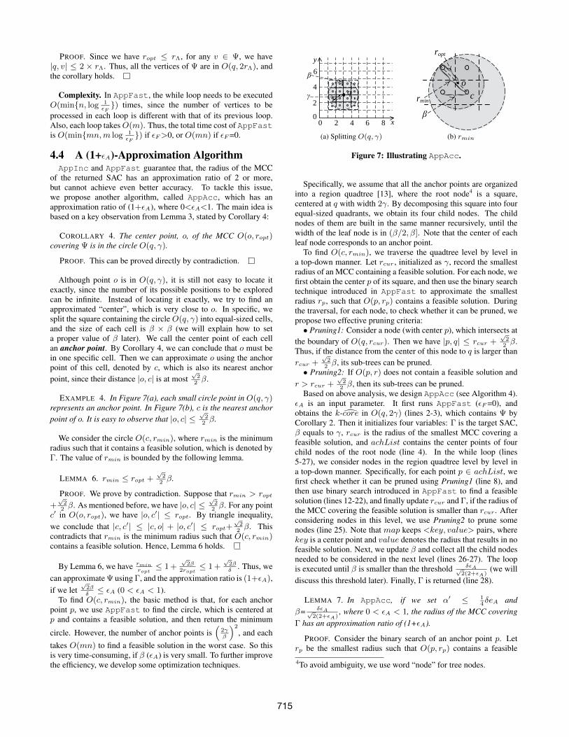
Although point o is in O(q, γ), it is still not easy to locate itexactly, since the number of its possible positions to be exploredcan be infinite. Instead of locating it exactly, we try to find anapproximated “center”, which is very close to o. In specific, wesplit the square containing the circle O(q, γ) into equal-sized cells,and the size of each cell is β × β (we will explain how to seta proper value of β later). We call the center point of each cellan anchor point. By Corollary 4, we can conclude that o must bein one specific cell. Then we can approximate o using the anchorpoint of this cell, denoted by c, which is also its nearest anchorpoint, since their distance |o, c| is at most

√2

2β.

EXAMPLE 4. In Figure 7(a), each small circle point in O(q, γ)represents an anchor point. In Figure 7(b), c is the nearest anchorpoint of o. It is easy to observe that |o, c| ≤

√2

2β.

We consider the circle O(c, rmin), where rmin is the minimumradius such that it contains a feasible solution, which is denoted byΓ. The value of rmin is bounded by the following lemma.

LEMMA 6. rmin ≤ ropt +√

22β.

PROOF. We prove by contradiction. Suppose that rmin > ropt

+√

22β. As mentioned before, we have |o, c| ≤

√2

2β. For any point

c′ in O(o, ropt), we have |o, c′| ≤ ropt. By triangle inequality,we conclude that |c, c′| ≤ |c, o| + |o, c′| ≤ ropt+

√2

2β. This

contradicts that rmin is the minimum radius such that O(c, rmin)contains a feasible solution. Hence, Lemma 6 holds.

By Lemma 6, we have rminropt

≤ 1 +√

2β2ropt

≤ 1 +√

2βδ

. Thus, wecan approximate Ψ using Γ, and the approximation ratio is (1+εA),if we let

√2βδ≤ εA (0 < εA < 1).

To find O(c, rmin), the basic method is that, for each anchorpoint p, we use AppFast to find the circle, which is centered atp and contains a feasible solution, and then return the minimum

circle. However, the number of anchor points is(

2γβ

)2

, and each

takes O(mn) to find a feasible solution in the worst case. So thisis very time-consuming, if β (εA) is very small. To further improvethe efficiency, we develop some optimization techniques.

42 60 8

2

4

6

Q

A

B C

D

0x

y

E

FG

H

I

r1

r2

u

l

r

δ

≤α

Q

42 60 8

2

4

6

Q

A

B C

D

0x

y

E

FG

H

I

γ

δ

l

u

qr

δl

u

qr

δ

42 60 8

2

4

6

q

0x

y

γ

β

rmin

ropt

oβ

c

β

o

c

r+

r-

f

42 60 8

2

4

6

Q

A

B C

D

0x

y

E

FG

H

I

r1

r2

r3

42 60 8

2

4

6

Q

A

B C

D

0x

y

E

FG

H

I

r1

r2

u

l

r

δ

≤α

Q

42 60 8

2

4

6

Q

A

B C

D

0x

y

E

FG

H

I

γ

δ

l

u

qr

δl

u

qr

δ

42 60 8

2

4

6

q

0x

y

γ

β

rmin

ropt

o

β

c

β

o

c

r+

r-

f

42 60 8

2

4

6

Q

A

B C

D

0x

y

E

FG

H

I

r1

r2

r3

(a) Splitting O(q, γ) (b) rmin

Figure 7: Illustrating AppAcc.

Specifically, we assume that all the anchor points are organizedinto a region quadtree [13], where the root node4 is a square,centered at q with width 2γ. By decomposing this square into fourequal-sized quadrants, we obtain its four child nodes. The childnodes of them are built in the same manner recursively, until thewidth of the leaf node is in (β/2, β]. Note that the center of eachleaf node corresponds to an anchor point.

To find O(c, rmin), we traverse the quadtree level by level ina top-down manner. Let rcur , initialized as γ, record the smallestradius of an MCC containing a feasible solution. For each node, wefirst obtain the center p of its square, and then use the binary searchtechnique introduced in AppFast to approximate the smallestradius rp, such that O(p, rp) contains a feasible solution. Duringthe traversal, for each node, to check whether it can be pruned, wepropose two effective pruning criteria:• Pruning1: Consider a node (with center p), which intersects at

the boundary of O(q, rcur). Then we have |p, q| ≤ rcur +√

22β.

Thus, if the distance from the center of this node to q is larger thanrcur +

√2

2β, its sub-trees can be pruned.

• Pruning2: If O(p, r) does not contain a feasible solution andr > rcur +

√2

2β, then its sub-trees can be pruned.

Based on above analysis, we design AppAcc (see Algorithm 4).εA is an input parameter. It first runs AppFast (εF=0), andobtains the k-core in O(q, 2γ) (lines 2-3), which contains Ψ byCorollary 2. Then it initializes four variables: Γ is the target SAC,β equals to γ, rcur is the radius of the smallest MCC covering afeasible solution, and achList contains the center points of fourchild nodes of the root node (line 4). In the while loop (lines5-27), we consider nodes in the region quadtree level by level ina top-down manner. Specifically, for each point p ∈ achList, wefirst check whether it can be pruned using Pruning1 (line 8), andthen use binary search introduced in AppFast to find a feasiblesolution (lines 12-22), and finally update rcur and Γ, if the radius ofthe MCC covering the feasible solution is smaller than rcur . Afterconsidering nodes in this level, we use Pruning2 to prune somenodes (line 25). Note that map keeps <key, value> pairs, wherekey is a center point and value denotes the radius that results in nofeasible solution. Next, we update β and collect all the child nodesneeded to be considered in the next level (lines 26-27). The loopis executed until β is smaller than the threshold δεA√

2(2+εA)(we will

discuss this threshold later). Finally, Γ is returned (line 28).

LEMMA 7. In AppAcc, if we set α′ ≤ 14δeA and

β= δεA√2(2+εA)

, where 0 < εA < 1, the radius of the MCC coveringΓ has an approximation ratio of (1+εA).

PROOF. Consider the binary search of an anchor point p. Letrp be the smallest radius such that O(p, rp) contains a feasible

4To avoid ambiguity, we use word “node” for tree nodes.

715

Algorithm 4 Query algorithm: AppAcc1: function APPACC(G, q, k, εA)2: obtain Φ, δ and γ using AppFast;3: S ← vertices of the k-core, containing q, in O(q, 2γ);4: Γ← Φ, β ← γ, rcur ← γ, achList← center points;5: while β ≥ δεA√

2(2+εA)do

6: map← ∅;7: for each point p ∈ achList do8: if |p, q| ≤ rcur +

√2

2β then //Pruning1

9: Γp ← find an SAC in O(p, rcur +√

22β);

10: if Γp 6= ∅ then11: u← rcur +

√2

2β, l← δ

2, map.put(p, l);

12: while u ≥ l do13: r ← l+u

2;

14: Γ′p ← find an SAC in O(p, r);15: if Γ′p 6= ∅ then16: Γp ← Γ′p;17: if r − l ≤ α′ then break;18: u← max

v∈Γq|q, v|;

19: else20: map.put(p, l);21: if u− r ≤ α′ then break;22: l← min

v∈S∧v/∈O(p,r)|q, v|;

23: r ← radius of the MCC covering Γp;24: if r < rcur then rcur ← r; Γ← Γp;25: prune anchor points in map using Pruning2;26: β ← β/2;27: update anchor point list achList using map;28: return Γ;

solution. From the proof of Lemma 5, we can conclude that,r ≤ rp + α′ when the binary search stops. Then, we have

r

rp≤ 1 +

α′

rp≤ 1 +

α′

ropt≤ 1 +

2α′

δ. (4)

Let α′= 14δεA. Then we have 2α′

δ= εA

2, and r ≤

(1 + εA

2

)rp.

Consider the updated rcur after the binary search for all theanchor points. Then we have rcur ≤

(1 + εA

2

)rmin. Let rΓ be

the radius of the MCC covering Γ. By Lemmas 3 and 6, we have

rΓ

ropt≤ rcurropt

≤ 1 +εA2

+(2 + εA)

√2β

2δ. (5)

Let (2+εA)√

2β2δ

= εA2

. Then we have rΓropt

≤ 1 + εA,

if β= δεA√2(2+εA)

. Hence, the approximation ratio of AppAcc is

(1+εA), if we set the parameters α′= 14δεA and β= δεA√

2(2+εA).

Complexity. There are O(( 2γβ

)2)=O(( 1εA

)2) anchor points.Similar as that in AppFast, the binary search for each anchorpoint needs to be executed O(min{n, log 1

εA}) times. So the total

cost of AppAcc is O(m( 1εA

)2 ×min{n, log 1εA}).

4.5 The Advanced Exact AlgorithmThe design of previous algorithms provide us many useful

insights for developing more advanced exact algorithms. Forexample, Corollary 2 states that, the optimal solution Ψ is inO(q, 2γ). This implies that, we can first run AppInc, then onlyenumerate the vertex triples for vertices in O(q, 2γ), which is asubset of V . Similarly, we can find Ψ by Corollary 3 based on

42 60 8

2

4

6

Q

A

B C

D

0x

y

E

FG

H

I

r1

r2

u

l

r

δ

≤α

Q

42 60 8

2

4

6

Q

A

B C

D

0x

y

E

FG

H

I

γ

δ

l

u

qr

δl

u

qr

δ

42 60 8

2

4

6

q

0x

y

γ

β

rmin

ropt

o

β

c

β

o

c

r+

r-

f

42 60 8

2

4

6

Q

A

B C

D

0x

y

E

FG

H

I

r1

r2

r3

Figure 8: Illustrating the annular region in Exact+.

AppFast. Although these methods could be faster than Exact,they are still far from perfect, because the number of potentialfixed vertices in O(q, 2γ) may still be very large. In this section,we propose a very efficient exact algorithm based on AppAcc,called Exact+, which largely reduces the number of potentialfixed vertices, and thus improves the efficiency significantly.

Recall that, AppAcc approximates the center, o, of the MCCcovering Ψ by its nearest anchor point c, and |o, c| ≤

√2

2β. Also,

ropt is well approximated, i.e., rΓropt≤1 + εA, which implies that,

rΓ

1 + εA≤ ropt ≤ rΓ, (6)

where 0 < εA < 1. So the value of ropt is in a small interval,especially if εA is small.

Besides, for any fixed vertex, f , of the MCC of Ψ, its distance too (i.e., |f, o|) is exactly ropt. By triangle inequality, we have

|f, c| ≤ |f, o|+ |o, c| ≤ rΓ +

√2

2β, (7)

|f, c| ≥ |f, o| − |o, c| ≥ rΓ

1 + εA−√

2

2β. (8)

Let us denote the rightmost items of above two inequations by r+

and r respectively. Then, we conclude that, for any fixed vertex f ,its distance to c is in the range [r , r+]. If εA is very small, the gapbetween r+ and r , i.e., r+−r =rΓ(1− 1

1+εA)+√

2β, is also verysmall, which implies that the locations of the fixed vertices are in avery narrow annular region. Hence, a large number of vertices outof this annular region, which are not fixed vertices, can be prunedsafely. We illustrate this in Figure 8, in which the annular region isthe area in O(c, r+), but not in O(c, r ).

Based on above analysis, we design Exact+ (Algorithm 5). Itfirst runs AppAcc with a small value of εA (line 2). Note thatΨ is initialized as Γ, and S and rcur are updated by AppAcc.Then, it collects a set, T , of anchor points that are not pruned inthe last while loop of AppAcc (line 3). Finally, an empty set F1

is initialized (line 4). For each anchor point p, it finds the potentialfixed vertices by Eqs (7) and (8), and adds them into F1 (line 5).

Next, it considers the three vertex combinations. It considerseach vertex v1 ∈ F1 as a fixed vertex of an MCC, and its farthestfixed vertex v2 for this MCC. By Lemma 2, we have |v1, v2| ∈[√

3ropt, 2ropt]. So a set F2 of potential farthest fixed vertices iscollected (line 7). Next, it collects a set, F3, of the third fixedvertices (line 9). Finally, it computes the MCC fixed by threevertices from F1, F2 and F3 respectively, keeps the SAC with thesmallest MCC radius (lines 11-16) and returns it (line 17). Notethat r and r+ are also updated during the enumeration, .

Complexity. Exact+ consists of two phases: (1) pruning ofthe fixed vertices (lines 2-5) and (2) enumeration of three vertexcombinations (lines 6-16). As discussed before, Phase (1) takesO(m( 1

εA)2×min{n, log 1

εA}), while Phase (2) needsO(m|F1|3).

716

Thus, the total cost of Exact+ isO(m( 1εA

)2×min{n, log 1εA}+

m|F1|3). We will address the effect of εA on |F1| and theperformance of Exact+ in the experiments.

Algorithm 5 Query algorithm: Exact+1: function EXACT+(G, q, k, εA)2: run APPACC(G, q, k, εA);3: T ← anchor points in map of AppAcc;4: initialize F1 ← ∅;5: for p ∈ T do F1.add{v|r ≤ |p, v| ≤ r+ ∧ v ∈ S};6: for v1 ∈ F1 do7: F2 ← {v|

√3r ≤ |v1, v| ≤ 2rcur ∧ v ∈ F1};

8: for v2 ∈ F2 do9: F3 ← {v||v1, v| ≤ |v1, v2| ∧ v ∈ F1};

10: for v3 ∈ F3 do11: compute the MCC mcc of {v1, v2, v3};12: if mcc.radius < rcur then13: R← a set of vertices in mcc;14: if exist a k-core in G[R] then15: rcur ← mcc.radius;16: Ψ← this k-core;17: return Ψ;

5. EXPERIMENTAL RESULTSWe describe the setup in Section 5.1. Sections 5.2 and 5.3 report

the effectiveness and efficiency results of SAC search.

5.1 SetupDatasets. We consider four real datasets: Brightkite5, Gowalla5,

Flickr6 and Foursquare7. For all the datasets, each vertex representsa user and each link represents the friendship between two users.Both Brightkite dataset and Gowalla dataset contain a collectionof check-in data shared by users of Brightkite service and Gowallaservice. In particular, for Brightkite dataset, there are 4,491,143checkins collected during the period of Apr. 2008 - Oct. 2010on 772,783 distinct places. The Gowalla dataset contain 6,442,892checkins collected on 1,280,969 places. In Flickr dataset, we markthe user a location if she has taken a photo there. With respectto Brightkite dataset, we consider the users’ locations can be bothstatic (Sections 5.2.1, 5.2.2 and 5.3) and dynamic (Section 5.2.3).The static location associated with a user is the place she checks in(or takes photos) most frequently. The Foursquare dataset [26] isextracted from Foursqaure website, and the location of each user isher hometown position. Users without locations are shipped.

We have also performed experiments on synthetic datasets.We are not aware of any existing spatial graph data generators.Therefore, we create synthetic data in the following way. First,we use GTGraph8, a well-known graph generator, to generate a(non-spatial) graph first. We adopt the default parameter valuesof GTGraph. The degrees of the graph follow a power-lawdistribution, which is often exhibited in social networks. Togenerate the location of each graph vertex, we first randomly selecta vertex v and give it a random position in the [0, 1] × [0, 1]space. Then we place v’s neighbors at random positions, whosedistances follows a normal distribution with mean µ and standarddeviation σ. We repeat this step for other vertices, starting from v’sneighbors, until every vertex is associated with a location. We setµ=0.09 and σ=0.16; these values are derived from the Brightkite5http://snap.stanford.edu/data/index.html6https://www.flickr.com/7https://archive.org/details/201309 foursquare dataset umn8http://www.cse.psu.edu/˜madduri/software/GTgraph/

Table 4: Datasets used in our experiments.Type Name Vertices Edges d

Real

Brightkite 51,406 197,167 7.67Gowalla 107,092 456,830 8.53Flickr 214,698 2,096,306 19.5

Foursquare 2,127,093 8,640,352 8.12

SyntheticSyn1 30,000 300,000 20Syn2 400,000 4,000,000 20

Table 5: Parameter settings.Parameter Range Default

εF (AppFast) 0.0, 0.5, 1.0, 1.5, 2.0 0.5εA (AppAcc) 0.01, 0.05, 0.1, 0.5, 0.9 0.5

k 4, 7, 10, 13, 16 4θ 10-6, 10-5, 10-4, 10-3, 10-2 10-4

n 20%, 40%, 60%, 80%, 100% 100%

dataset. Following these settings, we create two spatial graphs ofdifferent sizes, namely Syn1 and Syn2.

The statistics of each dataset are summarized in Table 4, whered is the average degree. Without loss of generality, we normalizeall the locations of each dataset into the unit square [0, 1]2.

Parameters. We consider 5 parameters: εF (the parameterof AppFast), εA (the parameter of AppAcc), k (denoting theminimum degree), θ (the parameter of θ-SAC search), and thepercentage of vertices n. The ranges of the parameters and theirdefault values are shown in Table 5. The default values of εFand εA are set as 0.5, since these values practically result in goodapproximation ratios with reasonable efficiency. Note that whenvarying n for scalability testing, we randomly extract subgraphs of20%, 40%, 60%, 80% and 100% vertices of the original graph witha default value of 100%. When varying a certain parameter, thevalues for all the other parameters are set to their default values.

Queries. For each dataset, we randomly select 200 queryvertices with core numbers of 4 or more. Such a core numberconstraint ensures a meaningful community (at least 4-core)containing the query vertex. In the results reported in the following,each data point is the average result for these 200 queries. We usethe term “AppFast(ε)” (“AppAcc(ε)”) to denote the algorithmAppFast (AppAcc) with the parameter εF=ε (εA=ε). Weimplement all the algorithms in Java, and run experiments on amachine having a quad-core Intel i7-3770 3.40GHz processor and32GB of memory, with Ubuntu installed.

5.2 Effectiveness EvaluationIn this section, we first study the approximation ratios of

approximation algorithms, then compare SAC search with thestate-of-art methods, and finally show results on dynamic graphs.

5.2.1 Approximation RatioIn Figure 9, we report the theoretical and actual approximation

ratios of AppFast and AppAcc on Brightkite and Gowalladatasets. Note that if we set εF=0.0, the results of AppFastare the same with those of AppInc, so we do not reportresults of AppInc. We can see that, the actual approximationratios of AppFast and AppAcc are much smaller than thetheoretical approximation ratios. For example, when εF=2, thetheoretical approximation ratio of AppFast is 4.0, but its actualapproximation ratios are around 2.0 on these two datasets. Similarresults can be observed from AppAcc in Figure 9(b).

717

2 2.5 3 3.5 41

1.5

2

2.5

Theoretical approx. ratio

Act

ual a

ppro

x. r

atio

BrightkiteGowalla

1.01 1.05 1.1 1.5 1.91

1.02

1.04

1.06

1.08

1.1

Theoretical approx. ratio

Act

ual a

ppro

x. r

atio

BrightkiteGowalla

(a) AppFast (b) AppAcc

Figure 9: Approximation ratio.

5.2.2 Comparison with the State-of-the-ArtsIn this subsection, we show that SAC search returns communities

with higher spatial cohesiveness compared with the state-of-the-artcommunity retrieval methods: Global [29], Local [7] andGeoModu [4]. The first two methods are CS methods designedfor non-spatial graphs, while GeoModu is a CD method for spatialgraphs. We also compare it with θ-SAC search. We brieflyintroduce these algorithms as follows (Let q be a query vertex):• Global: it finds the k-core containing q.• Local: it expands and explores from q, until it forms a

subgraph whose minimum vertex degree is at least k.• GeoModu: it first redefines the weight of each edge of graphG

as ei,j = 1di,jµ

, where di,j=|vi, vj | and µ (1 or 2) is a decay factor,and then detects the communities using modularity maximization.Given a query vertex, we return the community which contains it.• θ-SAC search: it first performs BFS search onG starting at

q to find a set S of vertices, which are connected with q and in thecircle O(q, θ), and then returns the k-core containing q in G[S].

Both Global and Local use the minimum degree metricfor structure cohesiveness. GeoModu has two variants, i.e.,GeoModu(1) and GeoModu(2), as the typical values of µ are1 and 2. To measure the spatial cohesiveness of a community Gqwith MCC O(c, r), we introduce two metrics as follows:• radius: the value of radius r.• distPr: average pairwise distance of vertices of Gq .Intuitively, lower values of these metrics for a community imply

that it achieves higher spatial cohesiveness. To compare thesemethods, we consider both exact and approximation algorithms.We search communities using these algorithms and compute theaverage values of above metrics for these communities. We reportthe results on Brightkite and Gowalla datasets in Figure 10.

(a) radius (b) distPr

Figure 10: Comparison with existing CD and CS methods.

1. CS comparison. We see that Local performs betterthan Global, as it finds communities through local expansion.The vertices of communities returned by Global and Localspread in larger areas than those of SAC search methods. Forexample, the average radii of the MCCs covering the communitiesof Global and Local are respectively 50 and 20 times larger

10−6 10−5 10−4 10−3 10−20

20

40

60

80

100

θ

perc

enta

ge

BrightkiteGowallaFlickrFoursquare

(a) Percentage (b) Radius

Figure 11: Results of θ-SAC search.

than that of our approach. The main reason is that they overlookthe spatial locations. Note that although Gq is in the smallestMCC, Gq may not be the subgraph with the minimum number ofvertices satisfying the minimum degree metric. In other words, aproper subset of vertices in Gq may form a qualified community,which has the same MCC as that of SAC search. Among theSAC search methods, the exact algorithm Exact+ achieves betterspatial cohesiveness than approximation algorithms consistently.

2. CD comparison. Since GeoModu considers both linksand locations, the returned communities achieve better spatialcohesiveness than Global and Local. While the averageradius and distPr values of GeoModu are larger than thoseof SAC search, a non-trivial number of queries in GeoModureturn communities whose MCCs are smaller than those of SAC(e.g., 19% and 18% of queries whose communities returnedby GeoModu(1) are in MCCs with smaller radii than thoseof Exact+, in Brightkite and Gowalla datasets respectively).However, the structure cohesiveness of communities detected byGeoModu is weaker. For example, the corresponding averagedegrees of vertices in communities returned by GeoModu(1)and GeoModu(2) on Brightkite dataset are 2.2 and 1.1. This isbecause GeoModu partitions the graph into clusters using a globalcriterion, i.e., Geo-Modularity [4], which has no reference to thequery vertices. Thus, SAC search achieves higher structure andspatial cohesiveness than GeoModu.

3. Comparison with θ-SAC search. We vary the value of θin θ-SAC search, and compute the percentage of queries returningnon-empty subgraphs. Figure 11(a) reports the results. Noticethat the percentage is low when θ is small. This is because manyusers’ SACs are spread in large areas. Also, the percentage variesgreatly for different datasets. Thus, setting a proper value of θ isnot easy. In contrast, SAC search does require the specificationof θ, and it always returns an SAC, if there is any. For queriesreturning non-empty SACs, we compute the average radius ofMCCs covering these SACs. We also compute the average radiusfor MCCs of SACs found by Exact+. Figure 11(b) compares theirresults. We observe that the average radius of MCCs coveringSACs found by θ-SAC search is 5 to10 times larger than thatof Exact+. This means that SAC search achieves better spatialcohesiveness than this variant. Hence, SAC search is easier to beused, and also achieves higher spatial cohesiveness than θ-SAC.

In addition, we have tried another approach by simply extractingvertices within O(q, θ) as a community, in which there is nostructure cohesiveness requirement. We vary the value of θ andcompute the average degree of vertices in the communities. Theresults show that, the average degree is very low. For example,the average values on Brightkite dataset are 0.36 and 0.39, whenθ is 10-6 and 10-5 respectively. This implies that the communitymay not be a connected subgraph. Thus, only using locations isinsufficient for identifying communities. In contrast, SAC searchalways guarantees that each vertex in an SAC has a minimumdegree of k or more.

718

4 7 10 13 16

10−1

100

101

102

k

time

(s)

AppIncAppFast(0.0)AppFast(0.5)AppAcc(0.5)

4 7 10 13 16

100

102

k

time

(s)

AppIncAppFast(0.0)AppFast(0.5)AppAcc(0.5)

4 7 10 13 16100

101

102

103

k

time

(s)

AppIncAppFast(0.0)AppFast(0.5)AppAcc(0.5)

4 7 10 13 16

101

102

103

k

time

(s)

AppIncAppFast(0.0)AppFast(0.5)AppAcc(0.5)

4 7 10 13 16

101

102

103

k

time

(s)

AppIncAppFast(0.0)AppFast(0.5)AppAcc(0.5)

(a) Brightkite (approx.) (b) Syn1 (approx.) (c) Flickr (approx.) (d) Foursquare (approx.) (e) Syn2 (approx.)

4 7 10 13 16

101

102

103

104

105

k

time

(s)

ExactExact+

4 7 10 13 16

101

102

103

104

105

k

time

(s)

ExactExact+

4 7 10 13 16

102

103

104

105

k

time

(s)

ExactExact+

4 7 10 13 16101

102

103

104

105

k

time

(s)

ExactExact+

4 7 10 13 16101

102

103

104

105

k

time

(s)

ExactExact+

(f) Brightkite (exact) (g) Syn1 (exact) (h) Flickr (exact) (i) Foursquare (exact) (j) Syn2 (exact)

20% 40% 60% 80% 100%

10−2

10−1

100

percentage

time

(s)

AppIncAppFast(0.0)AppFast(0.5)AppAcc(0.5)

20% 40% 60% 80% 100%

10−2

100

102

percentage

time

(s)

AppIncAppFast(0.0)AppFast(0.5)AppAcc(0.5)

20% 40% 60% 80% 100%

100

102

percentage

time

(s)

AppIncAppFast(0.0)AppFast(0.5)AppAcc(0.5)

20% 40% 60% 80% 100%

100

101

102

103

percentage

time

(s)

AppIncAppFast(0.0)

AppFast(0.5)AppAcc(0.5)

20% 40% 60% 80% 100%10−2

100

102

percentage

time

(s)

AppIncAppFast(0.0)

AppFast(0.5)AppAcc(0.5)

(k) Brightkite (scalability) (l) Syn1 (scalability) (m) Flickr (scalability) (n) Foursquare (scalability) (o) Syn2 (scalability)

Figure 12: Efficiency evaluation.

5.2.3 Adaptability to Location ChangesWe now study the adaptability of location changes of SAC

search. We focus on “dynamic” spatial graphs, where vertices’locations change frequently. We consider Brightkite dataset, andassume the link relationships do not change. We first sort all thecheckin records in chronological order. Then, we divide them intotwo groupsR1 andR2, whereR1 contains records collected before2010 and R2 contains the remaining records. Finally, we computethe total travel distance of each user, by adding up the distancesbetween each consecutive pair of checkins, and select a set Q of100 query users, who travel the longest and have at least 20 friends.

To evaluate the adaptability of location changes for SAC search,we first go through checkin records in R1 and update users’locations according to their latest checkin timestamps. Then, foreach user q ∈ Q, we do the same operation for records inR2, and ifthe record was generated by q, we search her SAC using Exact+.Finally, we obtain a list of SACs, Lq={C1, C2, · · · , Cl}, whereCi(1≤i≤l) is an SAC found at the timestamp of the i-th checkinrecord, and l is the total number of q’s check-in records.

To measure the overlap of member sets and spatial areas betweentwo communities Ci and Cj , we define two metrics: communityjaccard similarity (CJS) and community area overlapping (CAO),based on the classical Jaccard similarity.

CJS(Ci, Cj) =V (Ci) ∩ V (Cj)

V (Ci) ∪ V (Cj), (9)

CAO(Ci, Cj) =A(Ci) ∩A(Cj)

A(Ci) ∪A(Cj), (10)

where V (Ci) is the member set of Ci and A(Ci) is the area of theMCC covering Ci. Notice that CJS(Ci, Cj) and CAO(Ci, Cj)range from 0 to 1. A smaller value of CJS (CAO) implies loweroverlapping of community member sets (spatial areas).

0.25 0.5 1 3 5 7 10 150.4

0.5

0.6

0.7

0.8

0.9

1

η (day)

Ave

rage

CJS

0.25 0.5 1 3 5 7 10 150.4

0.5

0.6

0.7

0.8

0.9

1

η (day)

Ave

rage

CA

O(a) CJS (b) CAO

Figure 13: Effectiveness on dynamic spatial graph.

To show how the values of CJS and CAO vary with time, weselect communities from Lq , where the time gap between eachpair of communities is at least η, and compute their CJS and CAOvalues. We report their average results in Figure 13, where η variesfrom 0.25 day to 15 days. From Figure 13(a), we can observe that,the CJS decreases as the time threshold increases. For example,after 6 hours, the CJS decreases to 75%. In Figure 13(b), similarresults can be observed for CAO. In addition, we plot the SACs oftwo users in Figure 2. Thus, these results well confirm that, SACsearch has high adaptability to location changes.

5.3 Efficiency Evaluation1. Effect of k for approximation algorithms. Figures 12(a)-(e)

report the results. We skip the results on Gowalla, due to thespace limitation. We can see that AppFast runs consistently fasterthan AppInc and AppAcc. For example, for the largest datasetFoursquare, AppFast(0.0) is at least two orders of magnitudefaster than AppInc, although they return the same SACs.AppFast(0.0) is 2 to 5 times faster than AppAcc(0.5). Thisis because AppFast has a lower time complexity. In addition, therunning time of AppFast decreases as the value of k increases.This is because O(q, δ) becomes larger as k increases, and findinga larger O(q, δ) tends to need less binary search.

719

The running time of AppInc increases clearly as the value of kgrows. The reason is that, for a larger value of k, the correspondingO(q, δ) is also larger. As it finds O(q, δ) starting from the queryvertex q incrementally, a larger value of k results in a higher cost.AppAcc(0.5) is slower than AppFast. This is because its

first step is to run AppFast and it needs extra effort to find smallerMCCs. Also, its time cost tends to be stable. As discussed before,the number of anchor points is mainly affected by εA. Since εAis always 0.5 for different k, the numbers of anchor points are thesame, and thus the running time remains stable.

2. Effect of k for exact algorithms. Figure 14(a) shows that theefficiency of Exact+ is not very sensitive to εA on all real datasetsexcept Foursquare. Figure 14(b) shows |F1| increases with εA; thatis, fewer vertices are pruned as εA grows. Recall in Sec. 4.5 thatExact+ is composed of two phases. When εA is small, the costof Phase (1) dominates the overall cost; as εA increases, the cost ofPhase (2) grows. Thus, there is a local minimum in Figure 14(a).In practice, a sensitivity test can be done to choose εA.

10−6

10−5

10−4

10−3

0

1000

2000

3000

4000

time(

s)

εA

BrightkiteGowallaFlickrFoursquare

10−6

10−5

10−4

10−3

0

10

20

30

40

50

the

size

of s

et F

1

εA

BrightkiteGowallaFlickrFoursquare

(a) Effect of εA on efficiency (b) Effect of εA on |F1|Figure 14: Effect of εA on the efficiency of Exact+.

Figures 12(f)-(j) show the results of exact algorithms (εA=10-4).We skip the results of Exact, if a single query takes more than 10hours. We can see that, Exact performs extremely slow, even onthe smallest dataset. This because it adopts an exhaustive search tofind Ψ, which enumerates all the three vertex combinations. Hence,it is really worth the effort to study more efficient algorithms.Exact+ is at least four orders of magnitude faster than Exact.

This is because, it uses AppAcc to find narrow annular regions,in which fixed vertices are supposed to be contained, and thusthe number of fixed vertices needed to be enumerated is reducedsignificantly. The performance of Exact+ either slightly increasesor decreases as the value of k increases. This is because, afterpruning with the annular regions, the numbers of fixed verticesleft may be different, but in general larger datasets have morefixed vertices, and thus more time cost is needed. In addition,since Exact+ runs AppAcc in the first step, it is slower than theapproximation algorithms, but it takes reasonable time, i.e., fewseconds, on moderate-size graphs like Brightkite and Syn1.

3. Scalability. We vary the percentage of vertices in allthe datasets to study the scalability of approximation algorithms.The results are reported in Figures 12(k)-(o). We can see that,AppInc, AppFast and AppAcc generally scale well with n.Their performance trends are similar with those discussed before.In addition, AppFast(0.0)scales slightly better than AppInc.

6. CONCLUSIONSIn this paper, we study online SAC search algorithms. We

propose two exact algorithms, and three efficient approximationalgorithms. Our experiments show that SAC search achieves highereffectiveness than the state-of-the-art CD and CS algorithms. Inthe future, we will examine other spatial cohesiveness measures(e.g., pair-wise vertex distances). We will study how to supportbatch processing for SAC search. We will also develop asystem prototype and collect user statistics, to perform qualitativecomparison among communities generated by different solutions.

AcknowledgmentsReynold Cheng, Yixiang Fang, Xiaodong Li, Siqiang Luo, and JiafengHu were supported by the Research Grants Council of HK (Project HKU17205115 and 17229116) and HKU (Projects 102009508 and 104004129).We would like to thank Dr. Mauro Sozio for his insightful comments.

7. REFERENCES[1] N. Armenatzoglou et al. A general framework for geo-social query

processing. In PVLDB, volume 6, pages 913–924, 2013.[2] M. Barthelemy. Spatial networks. Physics Reports, 499(1):1–101,

2011.[3] V. Batagelj and M. Zaversnik. An o(m) algorithm for cores

decomposition of networks. arXiv, 2003.[4] Y. Chen et al. Finding community structure in spatially constrained

complex networks. IJGIS, 29(6):889–911, 2015.[5] Y. Chon, N. D. Lane, F. Li, H. Cha, and F. Zhao. Automatically

characterizing places with opportunistic crowdsensing usingsmartphones. In UbiComp, pages 481–490, 2012.

[6] W. Cui et al. Online search of overlapping communities. InSIGMOD, pages 277–288, 2013.

[7] W. Cui et al. Local search of communities in large graphs. InSIGMOD, pages 991–1002, 2014.

[8] D. J. Elzinga and D. W. Hearn. The minimum covering sphereproblem. Management science, 19(1):96–104, 1972.

[9] J. Elzinga and D. W. Hearn. Geometrical solutions for some minimaxlocation problems. Transportation Science, 6(4):379–394, 1972.

[10] P. Expert et al. Uncovering space-independent communities in spatialnetworks. PNAS, 108(19):7663–7668, 2011.

[11] Y. Fang et al. Effective community search for large attributed graphs.In PVLDB, pages 1233–1244, 2016.

[12] Y. Fang et al. Scalable algorithms for nearest-neighbor joins on bigtrajectory data. TKDE, 28(3):785–800, 2016.

[13] R. A. Finkel and J. L. Bentley. Quad trees: a data structure forretrieval on composite keys. Acta informatica, 4(1):1–9, 1974.

[14] S. Fortunato. Community detection in graphs. Physics Reports,486(3):75–174, 2010.

[15] M. Girvan et al. Community structure in social and biologicalnetworks. PNAS, 99(12):7821–7826, 2002.

[16] D. Guo. Regionalization with dynamically constrained agglomerativeclustering and partitioning (redcap). IJGIS, 22(7):801–823, 2008.

[17] T. Guo et al. Efficient algorithms for answering the m-closestkeywords query. In SIGMOD, pages 405–418. ACM, 2015.

[18] J. Hu et al. Querying minimal steiner maximum-connected subgraphsin large graphs. In CIKM, pages 1241–1250. ACM, 2016.

[19] X. Huang et al. Approximate closest community search in networks.In PVLDB, pages 276–287, 2015.

[20] A. Lancichinetti et al. Limits of modularity maximization incommunity detection. Phy. Rev. E, 84(6):066122, 2011.

[21] R.-H. Li et al. Influential community search in large networks. InPVLDB, volume 8, pages 509–520, 2015.

[22] K. M. MacQueen et al. What is community? an evidence-baseddefinition for participatory public health. AJPH, 91(12):1929–1938,2001.

[23] P. Manchanda et al. Social dollars: the economic impact of customerparticipation in a firm-sponsored online customer community.Marketing Science, 34(3):367–387, 2015.

[24] N. Megiddo. Linear-time algorithms for linear programming in r3and related problems. In FOCS, pages 329–338, 1982.

[25] M. Newman et al. Finding and evaluating community structure innetworks. Physical review E, 69(2):026–113, 2004.

[26] M. Sarwat et al. Lars*: a scalable and efficient location-awarerecommender system. TKDE, 26(6):1384–1399, 2014.

[27] J. Scott. Social network analysis. Sage, 2012.[28] S. B. Seidman. Network structure and minimum degree. Social

networks, 5(3):269–287, 1983.[29] M. Sozio and A. Gionis. The community-search problem and how to

plan a successful cocktail party. In KDD, pages 939–948, 2010.[30] W. Zhang, J. Wang, and W. Feng. Combining latent factor model

with location features for event-based group recommendation. InKDD, pages 910–918, 2013.

720