Effect Size © The Author(s) 2011 in Single-Case Research ... · in Single-Case Research: A Review...

Behavior ModificationXX(X) 1 –20

© The Author(s) 2011Reprints and permission: http://www.sagepub.com/journalsPermissions.nav

DOI: 10.1177/0145445511399147http://bmo.sagepub.com

Effect Size in Single-Case Research: A Review of Nine Nonoverlap Techniques

Richard I. Parker1, Kimberly J. Vannest1, and John L. Davis1

Abstract

With rapid advances in the analysis of data from single-case research designs, the various behavior-change indices, that is, effect sizes, can be confusing. To reduce this confusion, nine effect-size indices are described and compared. Each of these indices examines data nonoverlap between phases. Similarities and differences, both conceptual and computational, are highlighted. Seven of the nine indices are applied to a sample of 200 published time series data sets, to examine their distributions. A generic meta-analytic method is pre-sented for combining nonoverlap indices across multiple data series within complex designs.

Keywords

effect size, intervention effectiveness, measurement, single-case research

1Texas A&M University, College Station

Corresponding Author:Richard I. Parker, 604 Harrington Office Building, TAMU Mail Stop: 4225, College Station, TX 77843-4225Email: [email protected]

2 Behavior Modification XX(X)

Nine Nonoverlap Techniques for Single-Case Research

Analysis of single-case research (SCR) data is receiving unprecedented atten-tion in recent years, largely due to the need to support evidence-based inter-ventions with an “effect size” or index of amount of improvement by the client (Jenson, Clark, Kircher, & Kristjansson, 2007; Kazdin, 2008; Odom, 2009). Greater attention is also due to the press for greater rigor in educational research by the Institute of Education Sciences (IES) that has recently targeted SCR methods (IES, 2010). The net impact is the rapid development of several types of analyses for SCR, including multilevel models (van den Noortgate & Onghena, 2003, 2008), advanced regression models (Allison & Gorman, 1993; Huitema & McKean, 2000), and simpler, distribution-free nonparametric models, notably data nonoverlap between phases (Ma, 2006; Parker & Vannest, 2009; Parker, Vannest, & Brown, 2009).

The number of nonoverlap methods for SCR has increased considerably over the past decade, and these methods can be easily confused. The purpose of this article is to reduce potential confusion by describing them together, with comparisons. Some of these methods are very similar and some are closely related to other well-known statistical summaries. This is not intended to be a critical review. All nonoverlap methods share the benefit of being visually accessible and blending well with visual analysis of graphed data. In addition, all methods are “distribution free,” that is, not requiring parametric assumptions about data distribution or scale type.

Another asset of all nonoverlap techniques is their ease of use. They all can be calculated with a pencil and straightedge from a data plot. Some appear more complex than others but after initial practice prove to be user friendly for con-sumers in schools and clinics. Greater complexity comes with calculating con-fidence intervals and p values for nonoverlap indices, but these inferential tools are not needed for most lower stakes decisions. This article is directed to field practitioners who value visual analysis, so discussion of p values and confidence intervals is primarily limited to referring the reader to relevant tables or computer packages. Discussion of calculation methods derives mainly from our experience calculating the indices on hundreds of data sets over the past 6 years.

Nonoverlap indices are more robust than indices of mean or median level shifts across phases. A mean level comparison works well only when the mean and standard deviation are a good summary of the score distribution (Siegel & Castellan, 1988; Wilcox, 2010). However, when data are heavily skewed, a mean is rarely a good summary and a median is superior (Sheskin, 2007). But

Parker et al. 3

even a median is not a good description for the odd-shaped data sets often seen in SCR (Scruggs & Mastropieri, 1998, 2001). SCR data may have no scores close to a calculated median and/or may have multiple modes. When neither a mean nor a median can fairly summarize a data set, a nonoverlap method is needed (Parker et al., 2009; Wilcox, 2010). Nonoverlap methods do not rely on means, medians, or modes but rather consider the individual values of all data points in pairwise comparisons across phases. Nonoverlap methods may be “complete,” that is, considering all data points equally, or not, for example, percentage of nonoverlapping data (PND; Scruggs, Mastropieri, & Casto, 1987), which relies only on one data point in Phase A (the highest). Nonoverlap methods may consist solely of nonoverlap or may mix nonoverlap with median calcula-tion, for example, percentage of data points exceeding the median (PEM; Ma, 2006), and the extended celeration line (ECL) method (White & Haring, 1980).

Despite their advantages, most nonoverlap methods (all but two of those reviewed in this article) have a distinct disadvantage, also borne by simple mean-shift and median-shift models: insensitivity to trend, especially positive baseline trend (Wolery, Busick, Reichow, & Barton, 2010). Most nonoverlap tests should not be applied indiscriminately to just any data series. Two data attributes should preclude applying simple nonoverlap methods: (a) presence of positive trend in the baseline phase and (b) presence of strong improvement trend in the intervention phase, which would be poorly captured by an index of level only (mean, median, or nonoverlap methods). The phrase “most non-overlap methods” is used because two of the nine methods (the oldest and the newest) do consider data trend.

This article also highlights a relationship between several nonoverlap indices and established statistical tests. This topic may not interest all readers, but the relationships between nonoverlap and statistical tests argue for greater respect for the nonoverlap techniques by the broader research community. This may help correct the misunderstanding that nonoverlap techniques are synonymous with visual analysis; they are not. Connections between nonoverlap and estab-lished statistical tests help defend visual analysis, which has long attended to data nonoverlap (Parsonson & Baer, 1978). It is obvious that visual judgments of trend and mean or median shift have statistical counterparts. But in the past, a statistical counterpart of visual judgments of non-overlap was not explicit. That has now changed, and this article seeks to remedy the misunderstanding.

Finally, this article offers rough guidelines for the values that can be expected from each nonoverlap index. Seven of the nine indices were applied to a con-venience sample of 200 unscreened, published data sets, and resulting values are reported. Although this sample is not large enough to offer definitive


benchmarks, it can at least indicate which summaries tend to be higher and lower. General guidelines are already published for some of the indices but never together in one place nor calculated on the same corpus of data sets.

Besides the nine methods covered in this article, three additional SCR nonoverlap indices were not included. Percentage reduction data (PRD; O’Brien & Repp, 1990) was excluded because it is a parametric, mean-based method, rather than nonoverlap. Percentage of zero data (PZD; Scotti, Evans, Meyer, & Walker, 1991) was also excluded because of the fact that it fits only certain scales and goals. Last, the percentage of data exceeding a median trend (PEM-T; Wolery et al., 2010) was not covered because it is identical to the original “ECL or ‘split middle’ line” (White & Haring, 1980).

Nine Nonoverlap IndicesEight of the nine nonoverlap indices, presented in order of their first publica-tion dates, are depicted graphically in Figure 1 (computation methods for all indices are available in Table 1): (a) ECL or “split middle” line (White & Haring, 1980), (b) PND (Scruggs et al., 1987), (c) percentage of all non-overlapping data (PAND; Parker, Hagan-Burke, & Vannest, 2007), (d) robust Pearson’s phi (Phi; Parker et al., 2007), (e) PEM (Ma, 2006), (f) robust improve-ment rate difference (IRD; Parker et al., 2009), (g) nonoverlap of all pairs (NAP; Parker & Vannest, 2009), (h) Kendall’s tau for nonoverlap between groups (Taunovlap; Parker, Vannest, Davis, & Sauber, in press), and (i) tau for nonoverlap with baseline trend control (Tau-U; Parker et al., in press). Tau-U is not represented in Figure 1 due to its use of monotonic trend correction, which we have not yet learned to depict graphically.

ECL or “split middle” line. This venerable method (White & Haring, 1980) is one of only two in the group of nine which can control positive Phase A trend as part of nonoverlap. Nonoverlap is defined as the proportion of Phase B data that are above a median slope plotted from Phase A data, but then extended into Phase B. White and Haring (1980) hand fit a “split middle” median line to Phase A data, but any other trend line, for example, a Tukey tri-split line (Tukey, 1977), would work as well. White and Haring’s ECL does, however, depend on a straight line and makes the assumption of data linearity in baseline. When using ECL, a chance-level score is 50%, so the obtained 86% in Figure 1a could be described as “36% points beyond chance.” But a more useful stan-dardized interpretation is possible by rescaling it to a 0 to 100 scale, by the formula: Result0-100 = (Result50-100 / .5) – 1. For the same Figure 1a results, the transformation is, .86 / .5 – 1 = .72, so when rescaled 0 to 100, the final index is 72% nonoverlap. The 72% is more interpretable and therefore more

Parker et al. 5

Figure 1. Illustrates eight separate analyses of the same data set using (a) Extended Celeration Line (b) PND, (c) PAND, (d) Phi, (e) PEM, (f) IRD, (g) NAP, and (h) Taunovlap. Note: Tau-U is not represented in this figure.


Table 1. Computation Summaries of Nine Nonoverlap Methods

Method Procedure Example analysis

ECL a. Linear trend plotted from Phase A data and then extended through Phase B.

b. With transparent ruler, count the number of data points in Phase B above trend line.

c. Create ratio of Phase B data frequencies above line over total Phase B data points.

d. Compare this ratio with expected ratio of 50%.

• Given obtained ratio 9/12, compared with expected ratio 6/12.

• Input to statistical test of one proportion.

• Results: proportion 9/12 = .75. p = .149.

PND a. Single highest data point in Phase A identified (Hi).

b. Transparent ruler helps identify Phase B data points above Hi.

c. Ratio of number of data points above Hi to Phase B total data points.

• Given 20 Phase B data points, if 17 are above Hi, then PND = 17/20 = 85%.

• No statistical tests available.

PAND a. Minimum number of data points removed from Phase A and/or Phase B to eliminate all overlap between phases.

b. Ratio of number of data points not removed to the total equals PAND.

• Given Ns for Phase A = 7 and for Phase B = 11.

• Given minimum removed data points = 5.

• PAND = (18 – 5) / 18 = .72.

Phi a. Minimum number of data points removed from Phase A and/or Phase B to eliminate all overlap between phases.

b. Half of that minimum number is used to create two ratios, for Phase A and B.

c. Two ratios are submitted in 2 × 2 table to cross-tabs analysis, yielding Phi.


• Given minimum removed data points = 5, so half = 2.5.

• Ratio for Phase A = 2.5 / (7 – 2.5), ratio for Phase B = (11 – 2.5) / 2.5.

• For 2.5 / 4.5 versus 8.5 / 2.5, Phi = .416.

PEM a. Horizontal median line is drawn through Phase A and extended through Phase B.

b. Calculate percentage of Phase B data above that extended line = PEM.

c. No statistical analysis is specified, but Mood’s median test would be appropriate.

• Given N for Phase B = 12.

• Given Phase A median line extended through Phase B, splitting nine data points above and three below.

• PEM = 9 / 12 = .75.

(continued)

Parker et al. 7

Table 1. (continued)

Method Procedure Example analysis

IRD a. Minimum number of data points removed from Phase A and/or Phase B to eliminate all overlap between phases.

b. Half of that minimum number is used to create two ratios, for Phases A and B.

c. Two ratios are submitted to a two proportions test, yielding risk difference (which is IRD).

Note: Identical results as for robust Phi, but from a proportions test, not cross-tabs.


• Given minimum removed data points = 5, so half = 2.5.

• Ratio for Phase A = 2.5 / (7 – 2.5), ratio for Phase B = (11 – 2.5) / 2.5.

• Two proportions test for 2.5 / 4.5 versus 8.5 / 2.5, IRD = .416.

NAP a. Enter phase (0/1) and score variables submitted to ROC analysis module, yielding “empirical AUC” = .875.

ora. Phase (0/1) and Score variables

submitted to Mann-Whitney U.b. Output includes large U and small U.c. Calculate NAP = UL / (UL + US).

• Given Phase A data: 3, 5, 4, 3; Phase B data: 4, 5, 7, 7.

• From Mann-Whitney: UL = 14, US = 2.

• NAP = 14 / (14 + 2) = 87.5%.

• From ROC analysis, empirical AUC = 87.5%

Taunovlap a. Number of contrasted pairs (no. of pairs) calculated as product of two Phase Ns.

b. Variables for Phase (0/1) and score submitted to KRC test.

c. KRC outputs Kendall’s score or “S”.d. Taunovlap = S / number of pairs.

• Given raw data: Phase A = 3, 3, 4, 5; Phase B = 4, 5, 6, 7, 7.

• Number of pairs = 4 × 5 = 20.

• KRC output: S = 16. • Taunovlap = S / number of pairs = .80.

Tau-U a. Number of contrasted pairs (no. of pairs) calculated as product of two Phase Ns.

b. Phase variable coded reverse time order for Phase A, and for Phase B, all with the next time value.

c. Score and specially coded phase variables submitted to KRC test.

d. KRC outputs Kendall’s score or “S”.e. Tau-U = S / number of pairs.

• Given raw data: Phase A = 3, 3, 4, 5; Phase B = 4, 5, 6, 7, 7 (same as immediately above).

• Number of pairs = 4 × 5 = 20.

• Phase variable coded: 4, 3, 2, 1; 5, 5, 5, 5, 5.

• KRC output: S = 11. • Tau-U = S / number of pairs = .55.

Note: ECL = extended celeration line; PND = percentage of nonoverlapping data; PAND = percentage of all nonoverlapping data; Phi = robust Pearson’s phi; PEM = percentage of Phase B exceeding the Phase A median; IRD = robust improvement rate difference; NAP = nonoverlap of all pairs; ROC = receiver operator characteristic curve; AUC = empirical area under the curve; Taunovlap = Kendall’s tau nonoverlap; KRC = Kendall’s rank correlation; Tau-U = nonoverlap with baseline trend control.


usable as a standardized measure of effect. Computation of the ECL and other methods are summarized in Table 1.

The valuable ECL method is periodically rediscovered. Most recently pub-lished as PEM-T (Wolery et al., 2010), the PEM (Ma, 2006) can also be viewed as a subtype of ECL. PEM and ECL are identical when there is no Phase A trend. Although PEM differs little from ECL, PEM is included in this article as a separate analysis.

PND. Although well-documented limitations exist and call for its abandon-ment (Kratochwill et al., 2010; Parker & Vannest, 2009), PND (Scruggs et al., 1987) is still widely used and thus included here for comparison. PND is inter-preted as the percentage of Phase B data exceeding the single highest Phase A data point. In Figure 1b, the highest Phase A data point is 26, and five of the seven Phase B are above it, so PND = 5 / 7 = 71.4%. PND led the field as the earliest pure nonoverlap method. It remains the most widely published and is the basis of at least 10 meta-analyses (Scruggs & Mastropieri, 2001). PND tends to correlate well with visual judgments (Parker et al., 2007) and is prob-ably the easiest of all methods to calculate. Hand calculation is straightforward on uncrowded data sets with help from a transparent ruler. PND can range from 0% to 100%, with interpretation guidelines offered by its authors: >70% for effective interventions, 50% to 70% for questionable effectiveness, and <50% for no observed effect (Scruggs & Mastropieri, [1998]). Yet, of all the nonoverlap methods, only PND lacks a known sampling distribution, which prevents infer-ence testing. It also is the only nonoverlap method that emphasizes a single score in Phase A. So, the usefulness is limited to those data series where Phase A has no positive outliers, as a single high score dictates results.

PAND. This index is conceptualized as the percentage of data remaining after removing the fewest data points that would eliminate all overlap. From Figure 1c, the fewest data points needing removal to eliminate all overlap equals 2 (circled in Figure 1c). PAND (Parker et al., 2007) equals the remaining data, divided by the total N: 11 / 13 = 85%. PAND is scaled from 50 to 100, where 50% is chance level. To convert to a 0 to 100 scale, ([PAND / .5] – 1), here ([.85 / .5] – 1) = .70. PAND was designed to provide nonoverlap with a well-established effect size (Phi), though probably not a high priority with many visual analysts. Phi, the correlation coefficient for 2 × 2 tables, is the next method described. At its inception in 2007, two PAND calculation methods were presented, the first based on Excel sorting and the second based on visual scrutiny and hand cal-culation. The Excel sorting method has proved cumbersome and sometimes inexact, so now only the hand-calculation method should be followed.

Phi. Phi (Parker et al., 2007) was intended to legitimize PAND with a well-reputed effect size. Phi and Phi2 are equivalent to R and R2 for categorical data,

Parker et al. 9

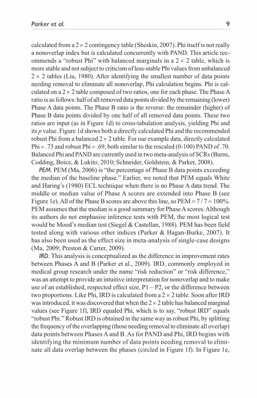
calculated from a 2 × 2 contingency table (Sheskin, 2007). Phi itself is not really a nonoverlap index but is calculated concurrently with PAND. This article rec-ommends a “robust Phi” with balanced marginals in a 2 × 2 table, which is more stable and not subject to criticism of less-stable Phi values from unbalanced 2 × 2 tables (Liu, 1980). After identifying the smallest number of data points needing removal to eliminate all nonoverlap, Phi calculation begins. Phi is cal-culated on a 2 × 2 table composed of two ratios, one for each phase. The Phase A ratio is as follows: half of all removed data points divided by the remaining (lower) Phase A data points. The Phase B ratio is the reverse: the remainder (higher) of Phase B data points divided by one half of all removed data points. These two ratios are input (as in Figure 1d) to cross-tabulation analysis, yielding Phi and its p value. Figure 1d shows both a directly calculated Phi and the recommended robust Phi from a balanced 2 × 2 table. For our example data, directly calculated Phi = .73 and robust Phi = .69, both similar to the rescaled (0-100) PAND of .70. Balanced Phi and PAND are currently used in two meta-analysis of SCRs (Burns, Codding, Boice, & Lukito, 2010; Schneider, Goldstein, & Parker, 2008).

PEM. PEM (Ma, 2006) is “the percentage of Phase B data points exceeding the median of the baseline phase.” Earlier, we noted that PEM equals White and Haring’s (1980) ECL technique when there is no Phase A data trend. The middle or median value of Phase A scores are extended into Phase B (see Figure 1e). All of the Phase B scores are above this line, so PEM = 7 / 7 = 100%. PEM assumes that the median is a good summary for Phase A scores. Although its authors do not emphasize inference tests with PEM, the most logical test would be Mood’s median test (Siegel & Castellan, 1988). PEM has been field tested along with various other indices (Parker & Hagan-Burke, 2007). It has also been used as the effect size in meta-analysis of single-case designs (Ma, 2009; Preston & Carter, 2009).

IRD. This analysis is conceptualized as the difference in improvement rates between Phases A and B (Parker et al., 2009). IRD, commonly employed in medical group research under the name “risk reduction” or “risk difference,” was an attempt to provide an intuitive interpretation for nonoverlap and to make use of an established, respected effect size, P1 – P2, or the difference between two proportions. Like Phi, IRD is calculated from a 2 × 2 table. Soon after IRD was introduced, it was discovered that when the 2 × 2 table has balanced marginal values (see Figure 1f), IRD equaled Phi, which is to say, “robust IRD” equals “robust Phi.” Robust IRD is obtained in the same way as robust Phi, by splitting the frequency of the overlapping (those needing removal to eliminate all overlap) data points between Phases A and B. As for PAND and Phi, IRD begins with identifying the minimum number of data points needing removal to elimi-nate all data overlap between the phases (circled in Figure 1f). In Figure 1e,


removing only 2 in Phase B would eliminate all overlap (an alternate solution would eliminate 2 in Phase A). Those 2 low data points are termed improved, so the calculated improvement rate for Phase B = 5 / 7 = 71% and for Phase A = 0 / 6 = 0%. IRD is the difference between these two rates: 71% – 0% = 71%. The preferable robust IRD is obtained by splitting the number of overlapping data points between phases, so instead of 5 / 7 – 0 / 6, the robust improvement rates are 6 / 7 – 1 / 6 = 86% – 17% = 69%, identical to robust Phi. Furthermore, a robust IRD also equals Cohen’s Kappa and Cramer’s V (Cliff, 1993). The universality of robust Phi = robust IRD should appeal to those of us seeking greater credibility for SCR data summaries within the broader research com-munity. Confidence intervals and p values for IRD are commonly available from statistics modules testing the difference between two proportions.

IRD is used in several meta-analyses of single-case designs (Davis & Vannest, in press; Ganz, Parker, & Benson, 2009; Vannest, Davis, Davis, Mason, & Burke, 2010; Vannest, Harrison, Temple-Harvey, Ramsey, & Parker, 2010).

NAP. NAP (Parker & Vannest, 2009) is interpreted as the percentage of all pairwise comparisons across Phases A and B, which show improvement across phases or, more simply, “the percentage of data which improve across phases.” Conceptually, NAP is a “complete” nonoverlap index as it individually com-pares all nA × nB data points. It is calculated as the number of improving or positive (Pos) pairs plus half of ties (.5 × Ties), divided by all pairs (Pairs): NAP = ([Pos + .5 × Ties] / Pairs). Unlike PAND/Phi and IRD, NAP is directly output from raw scores as “empirical area under the curve” (AUC) from a receiver operator characteristic curve (ROC) analysis. AUC is calculated by most full statistics programs, often in a “diagnostic tests” or ROC module. NAP also can be derived by simple calculation from Mann-Whitney U (see Table 1).

Although easily calculated by computer software, hand calculation requires only a little practice (see Figure 1f). First, the total of paired comparisons (Pairs) across phases is calculated as nA × nB = 6 × 7 = 42. Next, the “overlap zone” between phases is identified and within that zone only pairs that show decline (Neg) and ties (Ties) are counted. These two counts (Neg, Ties) are subtracted from number of Pairs to obtain the number of Pos. Figure 1f shows within the “overlap zone” Neg = 3 and Ties = 1, so Pos = 42 – 3 – 1 = 38. NAP is calculated as [Pos + .5 × no. of Ties) / no. of Pairs] = [(38 + .5) / 42 = .92]. NAP is scaled from 50% to 100%, where 50% is a chance-level result. To rescale NAP to a 0% to 100% scale, use NAP0-100 = 1 – (NAP50-100 / .5). For the example data, NAP0-100 = 1 – (.92 / .5) = .84. NAP is used in several recent meta-analysis of SCR (Bowman-Perrott et al., 2010; Davis, 2011; Davis & Vannest, in press).

Parker et al. 11

Taunovlap. Taunovlap (Parker et al., in press) is similar to NAP, in that it is based on all pairwise data comparisons made in a time-forward direction (see Figure 1h). Each pairwise comparison results in a decision of: Pos, Neg, or Tie, where Pos is score improvement from Phase A to B. Tau is the “percentage of nonoverlap minus overlap,” whereas NAP was simply “percentage of nonoverlap.” This difference is apparent in their respective formulas: Taunovlap = (Pos – Neg) / Pairs, whereas NAP = (Pos + .5 × Ties) / Pairs. For the example data (see Figure 1g), Taunovlap = (38 – 3) / 42 = .83.

As is the case with NAP, Taunovlap exists on a 50% to 100% scale, with 50% equaling chance-level results. Taunovlap can be rescaled from 0% to 100% using the formula given earlier: TAU0-100 = (Tau50-100 / .5) – 1. For the example data, Tau0-100 = (.83 / .5) – 1 = .66. The equivalence formulas for Taunovlap and NAP are (a) NAP = Taunovlap + ([no. of Neg + .5 × Ties] / Pairs) and (b) Taunovlap = NAP – [(no. of Neg + .5 × no. of Tie) / no. of Pairs].

Tau is obtained from either Kendall’s rank correlation (KRC) or from the Mann-Whitney U test, but both require minor hand calculations (Newson, 2001). To use KRC, dummy code “Phase 0/1” and then enter “phase” and “score” variables. Because KRC is not designed for dummy-coded variables, the Tau value output will not be correct. But the standard error, p value, and Kendall’s “S” (or “Score”) will be correct. So, Taunovlap needs to be hand calculated as follows: Taunovlap = S / Pairs. The denominator is obtained by multiplying the two Phase Ns: Pairs = NPhase A × NPhase B. As a side note, S = Pos – Neg.

To obtain Taunovlap from the Mann-Whitney U test, data are input normally: phase (dummy coded 0/1) and a score and variables. Alternatively, some statistics programs require two score columns, without a phase variable. The Mann-Whitney test outputs larger (UL) and smaller (US) values for U. A ratio involving these two equals Taunovlap, (UL – US) / (UL + US) = Taunovlap. For our example (UL – US) / (UL + US) = (38.5 – 3.5) / (38.5 + 3.5) = 35 / 42 = .83 = Taunovlap. The next section extends Taunovlap to control of baseline trend.

Tau-U. Tau-U (Parker et al., in press) extends Taunovlap to control for undesir-able positive baseline trend (monotonic trend). Monotonic trend is the upward progression of data points in any configuration, whether linear, curvilinear, or even in a mixed pattern of “fits and starts.”

For Tau-U, score and a specially-coded phase variable are submitted to a KRC module, as for Taunovlap. But the phase coding is different: for Phase A, input is a reverse time sequence and for Phase B, input is Phase B’s first time value, repeatedly. For our example, the phase coding is 6, 5, 4, 3, 2, 1 / 7, 7, 7, 7, 7, 7, 7. From the KRC analysis, the Tau output will not be accurate but Kendall’s S will be accurate, as will be the standard error and p value. Tau-U


must be hand calculated as S / number of Pairs. As shown earlier, the denomina-tor is the product of the two Phase Ns: number of Pairs = NPhase A × NPhase B = 6 × 7 = 42 The KRC analysis yields S = 31, so Tau-U = S / number of Pairs = 31 / 42 = .74. Note that .74 is smaller than Taunovlap = .83, reduced because of removal of the effects of Phase A trend. Described elsewhere at length (Parker et al., in press), this baseline trend control has the advantage of being conservative, avoiding extreme changes possible in controlling for linear trend.

Tau-U and ECL are the only two methods capable of controlling for Phase A trend. A major difference between the two is that ECL controls linear trend, whereas Tau-U controls monotonic trend. Also, ECL yields “percentage of data overlapping an extended median,” a less intuitive summary index than Tau-U’s “non-overlap after controlling for Phase A trend.” Finally, the statistical test from KRC for Tau-U is more powerful than the binomial test used for ECL.

Nonparametric “dominance” statistics. After PAND and IRD were published, commonalities were noted with established nonparametric statistics and that recognition led to the development of NAP. In fact, the method of “all pairwise score comparisons” is the hallmark of a group of nonparametric statistics with many equivalent names: “dominance,” “noninferiority,” “stochastic superiority,” “probabilistic statistic,” “P1 – P2,” and even “nonoverlap” (Huberty & Lowman, 2000). Dominance can be defined as the probability that a randomly selected score from one group (phase) will exceed that from a second group (phase). Key publications exploring dominance statistics are Cliff (1993); Grissom and Kim (2005); Huberty and Lowman (2000); Acion, Peterson, Temple, and Arndt (2006); D’Agostino, Campbell, and Greenhouse (2006); and Delaney and Vargha (2002).

Equivalence of established dominance statistics with nonoverlap in SCR brings greater credibility and a track record of methodological publications (see prior references). These include studies of bias, power, and precision, which show surprisingly strong results for tests such as Mann-Whitney U and KRC, both of which are based on the “S” distribution (Cliff, 1993; Huberty & Lowman, 2000; Wilcox, 2010). For example, Monte Carlo studies show their power to be 91% to 95% that of parametric t tests or ordinary least squares regression. This power estimate is for well-behaved data (normally distributed and with constant variance), which is not often available in SCR. For ill-behaved, nonnormal, skewed data, the nonparametric tests’ power can exceed 115% that of the standard parametric tests. This finding should increase the attractiveness of nonoverlap tests for typical SCR data.

Typical Nonoverlap ValuesTypical nonoverlap values from published SCR literature are available from various sources: (a) guidelines by authors, who often apply their techniques to

Parker et al. 13

dozens or even hundreds of studies informally; (b) field trials with a goal of identifying typical magnitudes; and (c) meta-analyses. To permit accurate com-parisons, however, these guidelines should be calculated from the same sample data. Table 2 presents such a summary from a convenience sample of 200 AB contrasts from more than 60 articles published in more than 15 different journals. The sample was collected without regard to effectiveness of interventions. Two thirds of the studies’ authors interpreted graphed results as indicating interven-tion success. White and Haring’s (1980) ECL and Tau-U were not included because among the nine indices only they considered Phase A trend, so would not be comparable to the other seven. However, the PEM index was included, which is identical to ECL in the absence of baseline trend. Separate visual-analysis ratings from three experienced raters (none were authors of the studies) classified 37% of the graphs as demonstrating small or negligible change, 22% as showing moderate change, and 40% as constituting a large amount of change.

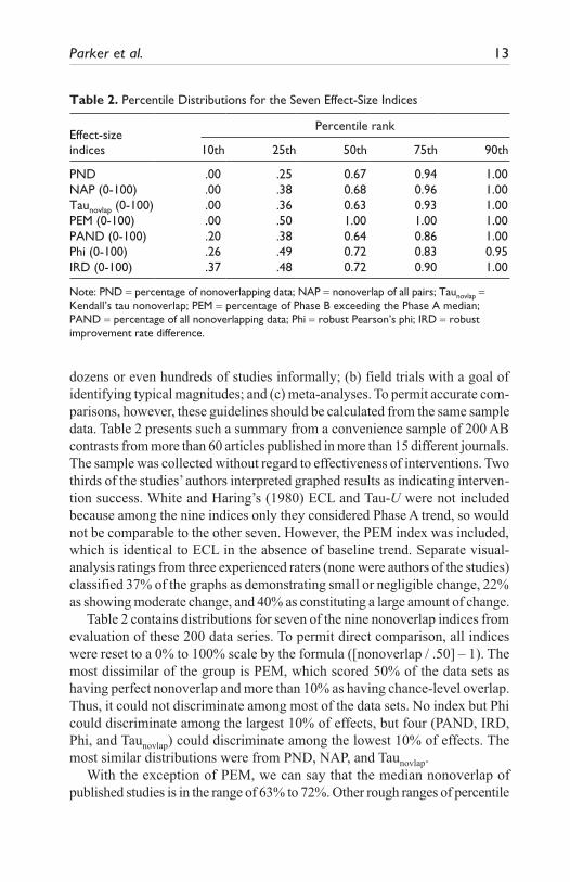
Table 2 contains distributions for seven of the nine nonoverlap indices from evaluation of these 200 data series. To permit direct comparison, all indices were reset to a 0% to 100% scale by the formula ([nonoverlap / .50] – 1). The most dissimilar of the group is PEM, which scored 50% of the data sets as having perfect nonoverlap and more than 10% as having chance-level overlap. Thus, it could not discriminate among most of the data sets. No index but Phi could discriminate among the largest 10% of effects, but four (PAND, IRD, Phi, and Taunovlap) could discriminate among the lowest 10% of effects. The most similar distributions were from PND, NAP, and Taunovlap.

With the exception of PEM, we can say that the median nonoverlap of published studies is in the range of 63% to 72%. Other rough ranges of percentile

Table 2. Percentile Distributions for the Seven Effect-Size Indices

Effect-size indices

Percentile rank

10th 25th 50th 75th 90th

PND .00 .25 0.67 0.94 1.00NAP (0-100) .00 .38 0.68 0.96 1.00Taunovlap (0-100) .00 .36 0.63 0.93 1.00PEM (0-100) .00 .50 1.00 1.00 1.00PAND (0-100) .20 .38 0.64 0.86 1.00Phi (0-100) .26 .49 0.72 0.83 0.95IRD (0-100) .37 .48 0.72 0.90 1.00

Note: PND = percentage of nonoverlapping data; NAP = nonoverlap of all pairs; Taunovlap = Kendall’s tau nonoverlap; PEM = percentage of Phase B exceeding the Phase A median; PAND = percentage of all nonoverlapping data; Phi = robust Pearson’s phi; IRD = robust improvement rate difference.


markers are 10th percentile, 0% to 37%; 25th percentile, 25% to 49%; 75th percentile, 0.83 to 0.96; and 90th percentile, 0.95 to 1.00. None of these dis-tributions include deterioration effects, which rarely occurred in published data.

Combining nonoverlap indices across multiple data series. A simple contrast of Phase A versus Phase B might be sufficient for a limited purpose, but published studies more often include several contrasts within a single design. In these cases, we may seek a single summary for the entire design. Combining Multiple A versus Multiple B contrasts for multiple baseline designs was described for PAND and Phi (Parker et al., 2007). But a more general approach is to use meta-analysis software to combine individual effects within a “fixed effects” model. We have found five free meta-analysis programs available for Internet download, of which the most useful for nonoverlap indices is WinPepi (Abramson, 2010; http://www.brixtonhealth.com/pepi4windows.html). WinPepi was built for medical researchers, who frequently use nonparametric analyses, so it offers a large number of nonparametric analyses. Simple proportions or percentages can be entered into WinPepi, each with their standard errors. WinPepi accepts IRD (two proportions) or a single proportion, and outputs an omnibus nonoverlap score, along with confidence intervals. The confidence intervals are narrower than for any of the individual phase contrasts because of the increased data points from all contrasts. Various weighting schemes are available for combin-ing individual contrasts, but a standard in meta-analysis is weighting by the inverse of the standard error of each contrast.

ConclusionsThis article sought to clarify similarities and differences among nine indices of nonoverlap for SCR data. The past half dozen years have seen a great increase in work toward better methods for analyzing SCR data. It is a priority of many, including the federal government’s IES, that SCR research become as rigorous and as valued as group research, to support evidence-based interventions (IES, 2010). Nonoverlap techniques require neither interval scales nor well-conforming data nor large data sets, which fits well with data typically produced in SCR research. Nonoverlap is based on the relative standing of individual data points, rather than means, medians, or even modes. In addition, one nonoverlap method (Tau-U) includes trend without requiring that the trend be linear.

Researchers should be mindful of the differences among nonoverlap tech-niques. First, although most techniques (PND, PAND/Phi, IRD, PEM, NAP, Taunovlap) cannot correct positive baseline trend, two (ECL and Tau-U) can do so. But the trends they control are quite different. ECL controls for linear trend, which is assumed to continue unabated without intervention. This assumption

Parker et al. 15

has been challenged (Scruggs & Mastropieri, 2001). In contrast, Tau-U controls monotonic trend, which is the tendency for scores to increase over time, in any configuration. Furthermore, Tau-U’s trend control is considerably more conservative than in ECL, as its effect is limited by Phase A length.

Another assumption made by only two methods (ECL and PEM) is that the median is a good summary of Phase A. This assumption is appropriate in cases where data show central tendency. But where data are bimodal, heavily skewed, or otherwise lacking in central tendency, reliance on the median (or mean) can distort results (Wilcox, 2010). Nonoverlap methods are more flexible in not relying on central tendency.

There are other important differences. Thirty years ago, nonoverlap techniques were regarded as a method to augment visual analysis, whereas now all nonoverlap methods but one (PND) are based on established sampling distributions. Therefore, confidence intervals and p values are available, so inference testing can become routine. Inference testing is especially important with short data series.

Adequate statistical power is a challenge in SCR with short data series, and the seven nonoverlap methods that permit inference testing are not equal in statistical power. Insufficient statistical power results in an inability to reliably identify smaller effects. Inadequate power also produces nonoverlap results with low precision, as shown by very large confidence intervals around obtained scores. Lowest power is afforded by ECL (binomial test) and PEM (Mood’s median test). Next in statistical power is Phi (chi-square test) and IRD (two proportions test). The greatest statistical power is available from NAP (AUC test), Taunovlap, and Tau-U (Kendall’s S test).

From a sample of 200 published AB designs, distribution similarities were noted among all seven of the methods not involving trend. With the exception of PEM, there was basic agreement on percentile markers. Mean scores for the sample averaged 63% to 72%, and at the 75th percentile scores were 83% to 96%. Greatest similarity was among PND, NAP, and Taunovlap. What may impress readers most is the magnitude of these nonoverlap values. Nonoverlap scores are considerably larger than scores from other parametric or nonpara-metric 0 to 1 scaled summaries. Smaller scores were obtained from Phi, which is not a nonoverlap index, though based on nonoverlap.

An attribute shared by all indices with the exception of Phi is insensitivity to results at the top end (here the largest 10%) of the distribution. For PEM, insensitivity was at a high level, that is, unable to distinguish among 50% of the sample. But insensitivity to even 10% would be a marked disadvantage if one were attempting to compare two successful interventions. This insensitivity is inherent in nonoverlap calculations, and the only apparent remedy seems to be to expand nonoverlap to include trend also. Though it could not be included in Table 2 because of slope corrections, Tau-U sensitivity exceeds all others.


Besides their differences, some of the nine indices are markedly similar or even identical. It was noted that ECL (White & Haring, 1980) is identical to the new PEM-T (Wolery et al., 2010) and that PEM (Ma, 2006) is subsumed under ECL. Also noteworthy is the close similarity of PAND, Phi, and IRD, all computed from a 2 × 2 matrix. In a balanced 2 × 2 matrix, Phi and IRD are the same. Also, quite similar are NAP and Taunovlap, as they are calculated the same way, except that Taunovlap subtracts nonoverlapping data, whereas NAP does not. They also differ in how ties found in paired comparisons are treated.

The identity of NAP and tau with the group of nonparametric “dominance statistics” offers new validation for nonoverlap as an effect size. The visual analysis practice of judging nonoverlap is now validated and supported by respected tests such as the Mann-Whitney U, KRC, and the ROC analysis. These dominance tests have equivalence formulas, and through those formulas, nonoverlap as a concept can be better understood and expanded. These con-nections are leading to an integrated, nonparamentric measure of nonoverlap and trend, as exemplified by Tau-U. Nonoverlap methods, as other SCR ana-lytic techniques, are improving rapidly and in a few years may show substantial improvements.

Declaration of Conflicting Interests

The author(s) declared no potential conflicts of interests with respect to the authorship and/or publication of this article.

Funding

The author(s) received no financial support for the research and/or authorship of this article.

References

Abramson, J. H. (2010). Programs for epidemiologists-Windows version (WinPepi) [Computer software]. Retrieved from http://www.brixtonhealth.com/pepi4windows .html

Acion, L., Peterson, J., Temple, S., & Arndt, S. (2006). Probabilistic index: An intui-tive nonparametric approach to measuring the size of treatment effects. Statistics in Medicine, 25, 591-602.

Allison, D. B., & Gorman, B. S. (1993). Calculating effect sizes for meta-analysis: The case of the single case. Behavior, Research, and Therapy, 31, 621-631.

Bowman-Perrott, L., Vannest, K. J., Williams, L. B., Aguirre, C. A., Hemrick-DeMarin, S., & Davis, H. S. (2011). Class wide peer tutoring: A meta analysis. Manuscript in preparation.

Parker et al. 17

Burns, M. K., Codding, R. S., Boice, C. H., & Lukito, G. (2010). Meta-analysis of acquisition and fluency math interventions with instructional and frustration level skills: Evidence for a skill-by-treatment interaction. School Psychology Review, 39, 69-83.

Cliff, N. (1993). Dominance statistics: Ordinal analyses to answer ordinal questions. Psychological Bulletin, 114, 494-509.

D’Agostino, R. B., Campbell, M., & Greenhouse, J. (2006). Noninferiority trials: Continued advancements in concepts and methodology. Statistics in Medicine, 25, 1097-1099.

Davis, J. L. (2011). Effective intervention for behavior through self monitoring: A meta-analysis. Manuscript in preparation.

Davis, J. L., & Vannest, K. J. (in press). Effect size for single case research a replica-tion and re-analysis of an existing meta-analysis. Remedial and Special Education.

Delaney, H. D., & Vargha, A. (2002). Comparing several robust tests of stochastic equality with ordinally scaled variables and small to moderate sized samples. Psychological Methods, 7, 485-503.

Ganz, J. B., Parker, R., & Benson, J. (2009). Impact of the picture exchange commu-nication system: Effects on communication and collateral effects on maladaptive behaviors. Augmentative and Alternative Communication, 25, 250-260.

Grissom, R. J., & Kim, J. J. (2005). Effect sizes for research: A broad practical approach. Mahwah, NJ: Lawrence Erlbaum.

Huberty, C. J., & Lowman, L. L. (2000). Group overlap as a basis for effect size. Educational and Psychological Measurement, 60, 543-563.

Huitema, B. E., & McKean, J. W. (2000). Design specification issues in time-series intervention models. Educational and Psychological Measurement, 60, 38-58.

Institute of Education Sciences. (2010, May 12). NCSER hosts meeting to discuss data analysis challenges [Web Post]. Retrieved from http://ies.ed.gov/whatsnew/newsletters/jan10.asp?index=roundncser

Jenson, W. R., Clark, E., Kircher, J. C., & Kristjansson, S. D. (2007). Statistical reform: Evidence-based practice, meta-analyses, and single subject designs. Psychology in the Schools, 44, 483-493.

Kazdin, A. E. (2008). Evidence-based treatment and practice: New opportunities to bridge clinical research and practice, enhance knowledge base, and improve patient care. American Psychologist, 63, 149-159.

Kratochwill, T. R., Hitchcock, J., Horner, R. H., Levin, J. R., Odom, S. L., Rindskopf, D. M., & Shadish, W. R. (2010). Single-case designs technical docu-mentation. Retrieved from http://ies.ed.gov/ncee/wwc/pdf/wwc_scd.pdf

Liu, R. (1980) A note on phi-coefficient comparison. Research in Higher Education, 13, 3-8.


Ma, H. H. (2006). An alternative method for quantitative synthesis of single-subject researches: Percentage of data points exceeding the median. Behavior Modification, 30, 598-617.

Ma, H. H. (2009). The effectiveness of intervention on the behavior of individuals with autism: A meta-analysis using percentage of data points exceeding the median of baseline Phase (PEM). Behavior Modification, 3, 339-359.

Newson, R. (2001). Parameters behind “nonparametric” statistics: Kendall’s Tau, Somers’ D and median differences. Stata Journal, 1, 1-20.

O’Brien, S., & Repp, A. C. (1990). Reinforcement-based reductive procedures: A review of 20 years of their use with persons with severe or profound retardation. Journal of the Association for Persons With Severe Handicaps, 15, 148-159.

Odom, S. L. (2009). The tie that binds: Evidence-based practice, implementation science, and outcomes for children. Topics in Early Childhood Special Education, 29, 53-61.

Parker, R. I., & Hagan-Burke, S. (2007). Single case research results as clinical out-comes. Journal of School Psychology, 45, 637-653.

Parker, R. I., Hagan-Burke, S., & Vannest, K. J. (2007) Percent of all nonover-lapping data PAND: An alternative to PND. Journal of Special Education, 40, 194-204.

Parker, R. I., & Vannest, K. J. (2009). An improved effect size for single case research: NonOverlap of All Pairs (NAP). Behavior Therapy, 40, 357-367.

Parker, R. I., Vannest, K. J., & Brown, L. (2009). The improvement rate difference for single case research. Exceptional Children, 75, 135-150.

Parker, R. I., Vannest, K. J., Davis, J. L., & Sauber, S. B. (in press). Combining non-overlap and trend for single case research: Tau-U. Behavior Therapy.

Parsonson, B. S., & Baer, D. M. (1978). The analysis and presentation of graphic data. In T. R. Kratochwill (Ed.), Single-subject research: Strategies for evaluating change (pp. 101-165). New York, NY: Academic Press.

Preston, D., & Carter, M. (2009). A review of the efficacy of the picture exchange com-munication system intervention. Journal of Autism and Developmental Disorders, 39, 1147-1486.

Schneider, N., Goldstein, H., & Parker, R. (2008). Social skills interventions for chil-dren with autism: A meta-analytic application of percentage of all nonoverlapping data (PAND). Evidence-Based Communication Assessment and Intervention, 2, 152-162.

Scotti, J. R., Evans, I. M., Meyer, L. H., & Walker, P. (1991). A meta-analysis of intervention research with problem behavior: Treatment validity and standards of practice. American Journal on Mental Retardation, 96, 233-256.

Scruggs, T. E., & Mastropieri, M. A. (1998). Summarizing single-subject research: Issues and applications. Behavior Modification, 22, 221-242.

Parker et al. 19

Scruggs, T. E., & Mastropieri, M. A. (2001). How to summarize single-participant research: Ideas and applications, Exceptionality, 9, 227-244.

Scruggs, T. E., Mastropieri, M. A., & Casto, G. (1987). The quantitative synthesis of single subject research: Methodology and validation. Remedial and Special Education, 8, 24-33.

Sheskin, D. J. (2007). Handbook of parametric and nonparametric statistical procedures (4th ed.). Boca Raton, FL: Chapman and Hall.

Siegel, S., & Castellan, N. J., Jr. (1988). Nonparametric statistics for the behavioral sciences (2nd ed.). New York, NY: McGraw-Hill.

Tukey, J. W. (1977). Exploratory data analysis. Reading, MA: Addison-Wesley-Longman.van den Noortgate, W., & Onghena, P. (2003). Hierarchical linear models for the quan-

titative integration of effect sizes in single case research. Behavior Research Methods, Instruments & Computers, 35, 1-10.

van den Noortgate, W., & Onghena, P. (2008). A multilevel meta-analysis of single-subject experimental design studies. Evidence-Based Communication Assessment and Intervention, 2, 142-158.

Vannest, K. J., Davis, J. L., Davis, C. R., Mason, B. A., & Burke, M. D. (2010). Effective intervention with a daily behavior report card: A meta-analysis. School Psychology Review, 39, 654-672.

Vannest, K. J., Harrison, J. R., Temple-Harvey, K., Ramsey, L., & Parker, R. I. (2010). Improvement rate differences of academic interventions for students with emotional and behavioral disorders. Remedial and Special Education. doi:10.1177/0741932510362509

White, O. R., & Haring, N. G. (1980). Exceptional teaching: A multimedia training package. Columbus, OH: Merrill.

Wilcox, R. R. (2010). Fundamentals of modern statistical methods: Substantially improving power and accuracy (2nd ed.). New York, NY: Springer.

Wolery, M., Busick, M., Reichow, B., & Barton, E. (2010). Comparison of overlap methods for quantitatively synthesizing single-subject data. Journal of Special Education, 44, 18-28.

Bios

Richard I. Parker, PhD, is in the educational psychology department at Texas A&M University. He has taught general and special education, has been a school psycholo-gist, and served as director of special education. His most recent research foci are single case research methods, progress-monitoring measurement issues, and defensible non-parametric analyses.

Kimberly J. Vannest is an associate professor in the Department of Educational Psychology, Special Education at Texas A&M University. Her research interests are


in determining effective interventions for children and youth with or at risk for emo-tional and behavioral disorders, including teacher behaviors and measurement.

John L. Davis is a doctoral student in the school psychology program at Texas A&M University. His research interests include measurement considerations in progress monitoring and acceptability of intervention protocols in schools.

Effect Size © The Author(s) 2011 in Single-Case Research ... · in Single-Case Research: A Review...

Documents

Transcript of Effect Size © The Author(s) 2011 in Single-Case Research ... · in Single-Case Research: A Review...