Effect Of Weak Adhesion Interface On Mechanical And ...
82
University of South Carolina Scholar Commons eses and Dissertations 2018 Effect Of Weak Adhesion Interface On Mechanical And Dielectric Properties Of Composite Materials Prashant Katiyar University of South Carolina Follow this and additional works at: hps://scholarcommons.sc.edu/etd Part of the Mechanical Engineering Commons is Open Access esis is brought to you by Scholar Commons. It has been accepted for inclusion in eses and Dissertations by an authorized administrator of Scholar Commons. For more information, please contact [email protected]. Recommended Citation Katiyar, P.(2018). Effect Of Weak Adhesion Interface On Mechanical And Dielectric Properties Of Composite Materials. (Master's thesis). Retrieved from hps://scholarcommons.sc.edu/etd/4734
Transcript of Effect Of Weak Adhesion Interface On Mechanical And ...

University of South CarolinaScholar Commons
Theses and Dissertations
2018
Effect Of Weak Adhesion Interface On MechanicalAnd Dielectric Properties Of Composite MaterialsPrashant KatiyarUniversity of South Carolina
Follow this and additional works at: https://scholarcommons.sc.edu/etd
Part of the Mechanical Engineering Commons
This Open Access Thesis is brought to you by Scholar Commons. It has been accepted for inclusion in Theses and Dissertations by an authorizedadministrator of Scholar Commons. For more information, please contact [email protected].
Recommended CitationKatiyar, P.(2018). Effect Of Weak Adhesion Interface On Mechanical And Dielectric Properties Of Composite Materials. (Master's thesis).Retrieved from https://scholarcommons.sc.edu/etd/4734

EFFECT OF WEAK ADHESION INTERFACE ON MECHANICAL AND DIELECTRIC
PROPERTIES OF COMPOSITE MATERIALS
by
Prashant Katiyar
Bachelor of Science
Barkatullah University, 2009
Submitted in Partial Fulfillment of the Requirements
For the Degree of Master of Science in
Mechanical Engineering
College of Engineering and Computing
University of South Carolina
2018
Accepted by:
Prasun Majumdar, Director of Thesis
Xinyu Huang, Second Reader
Cheryl L. Addy, Vice Provost and Dean of the Graduate School

ii
© Copyright by Prashant Katiyar, 2018
All Rights Reserved.

iii
ACKNOWLEDGEMENTS
First of all, I would like to express my earnest gratitude to Dr. Prasun Majumdar
for his continued guidance throughout my research endeavors. I’m forever inspired by his
drive to learn something new every day and his vast knowledge in the field of advanced
materials. I’d like to thank Dr. Xinyu Huang for being a part of my thesis defense
committee.
Next, this research would not have been possible without the unending
encouragement and assistance from my colleagues – Shriram Bobbili, Alice Arnold and
Cameron Wilkes.
Lastly, I would like to thank my family, especially my sister for motivating me and
supporting me throughout my studies here in USC.

iv
ABSTRACT
Interfaces are often the most critical part of the heterogeneous materials and their
structures. Such interfaces appear a multiple length scales and significantly affect bulk
properties in different material systems. Fiber reinforced composite materials are one such
example of heterogeneous materials with interfaces at constituent scale (fiber-matrix
interface and interphase) to laminate scale (secondary adhesive joints). Manufacturing
induced defects and subsequent in-service damage at these interfaces can severely affect
the durability of fiber reinforced laminated composite materials and their joints. In addition
to lamination process, defects can also form during secondary joining process (e.g.,
adhesive bonding and repair) which can be very detrimental to the performance of the
composite structure as it can become the “weak link”. Adhesive bonding has wide
applications in different disciplines including bio-medical, energy, automotive, civil and
aerospace structural composites. With growing popularity of adhesive bonding,
manufacturing defects at the interfaces of joints have attracted increased attention of many
researchers in the recent years. Although significant progress has been made in detecting
specific types of defects such as voids and large debonding using different NDE methods,
there is a lack of understanding of so called “zero volume” defects which forms a weak
interface. The purpose of this study is to examine the role of defects at the adhesive-to-
laminate interface on multi-physical properties, and specifically understand how a weak
interface may affect mechanical durability.

v
In this study, a multi-faceted approach has been taken to understand fundamental
scientific challenge of surface properties and its implications on bonded interface.
Controlled experiments have been designed to create weak interface by different surface
modification technique and validated with indirect measurement of work of adhesion.
Using broadband dielectric spectroscopy (BbDS) technique, the effect of surface
modification on dielectric properties are quantified. This modification is then translated in
formation of a truly “weak interface” with “zero volume” unlike a traditional disbond or
delamination type scenario. The laminated composite joint is then studied for both
mechanical and dielectric property changes due to the formation of weak interface. Carbon
fiber reinforced laminate and epoxy adhesive were taken as test bench material systems
although the fundamental focus is not on the material itself but the interface.
Interface strength of bonded joint was determined experimentally and
quantitatively linked to dielectric properties. Several analytical models were developed to
understand the effect of weak interface on dielectric properties and results demonstrate that
the model captures observed experimental trend of property changes. Moreover, failure of
bonded structure under tension loading was also predicted with analytical tools available
in the literature and it was observed that only shear dominated brittle fracture represents
the weak interface adequately. This is an interesting shift as a strong joint will show
ductility in terms of both shear and peel stresses due to adherend bending effect. Details of
experimental results and analyses of weak interface have been included in this thesis.

vi
TABLE OF CONTENTS
ACKNOWLEDGEMENTS ........................................................................................................ iii
ABSTRACT .......................................................................................................................... iv
LIST OF FIGURES ................................................................................................................ vii
LIST OF TABLES ....................................................................................................................x
CHAPTER 1: INTRODUCTION AND LITERATURE REVIEW........................................................1
CHAPTER 2: BACKGROUND ON EXPERIMENTAL METHODS .................................................16
CHAPTER 3: EFFECT OF SURFACE MODIFICATION ...............................................................20
CHAPTER 4: INTERFACIAL DEFECT AND PROPERTIES OF BONDED LAMINATES ..................37
CHAPTER 5: MECHANICAL DURABILITY OF JOINTS WITH WEAK INTERFACE .....................47
CHAPTER 6: ANALYTICAL FORMULATION OF DIELECTRIC AND MECHANICAL PROPERTIES
OF BONDED JOINTS ....................................................................................................58
CHAPTER 7: CONCLUSIONS AND FUTURE WORK ................................................................70

vii
LIST OF FIGURES
Figure 1.1 Modes of failure in adhesive bonds ....................................................................6
Figure 3.1 Contact angles of different kind of surfaces. ....................................................22
Figure 3.2 laminate surfaces after Release agent application ............................................24
Figure 3.3 Contact angle pictures ......................................................................................25
Figure 3.4 Images of specimen C taken at different time ..................................................26
Figure 3.5. Contact angle pictures .....................................................................................27
Figure 3.6 Adhesive ability to wet rough surface ..............................................................28
Figure 3.7 Smooth (left) and rough (right) surfaces ..........................................................29
Figure 3.9. Imaginary Permittivity as a function of frequency before and after applying
FRA on laminate surface ...................................................................................................33
Figure 3.10. Change in AC impedance function of frequency before and after applying
FRA on laminate surface ...................................................................................................33
Figure 3.11. Change in imaginary permittivity as a function of frequency before and after
applying FRA on laminate surface ....................................................................................34
Figure 3.12 Change in AC impedance function of frequency before and after applying
FRA on laminate surface ...................................................................................................34
Figure 3.13 Change in dielectric properties as a function of frequency with different
surface defects ....................................................................................................................35
Figure 4.1 SpeedMixer.......................................................................................................40
Figure 4.2. Schematic of overlap joint preparation with Teflon/release film ....................41
Figure 4.3. Adhesively bonded overlap joint (right) and schematic of same (left) ...........42
Figure 4.4. Change in permittivity as a function of frequency
of different surface defects.................................................................................................43

viii
Figure 4.5 Change in capacity as a function of frequency of different surface defects .....44
Figure 4.6 Change in dielectric properties as a function of frequency with different
surface defects ....................................................................................................................44
Figure 4.7 Change in real permittivity with increasing percentage of release film in
overlap joint .......................................................................................................................45
Figure 4.8 Change in normalized properties with increasing percentage of release film in
overlap joint .......................................................................................................................46
Figure 4.9 Change in normalized properties with increasing percentage of release film in
overlap joint .......................................................................................................................46
Figure 5.1. “weak” (top) and undamaged (middle) and image of single lap joint (bottom)
as per ASTM standards ......................................................................................................49
Figure 5.2. Cross section of Single lap joint (left) and experimental setup for tensile
testing .................................................................................................................................50
Figure 5.3. Load vs displacement response of weak joint (top) and undamaged joint ......51
Figure 5.4. Average shear strength of weak and undamaged specimens...........................52
Figure 5.5 Specimens after failure in MTS with weak joints ............................................53
Figure 5.6. specimen-electrode assembly for BbDS ..........................................................53
Figure 5.7. MicroXTC-400 ................................................................................................54
Figure 5.8. Real and imaginary part of frequency as a frequency function .......................55
Figure 5.9 Change in AC impedance at 0.1 Hz of lap joint due to interfacial defect ........55
Figure 5.10. Change in normalized properties in weak joints specimens ..........................56
Figure 5.11. X-ray images of single lap joint specimen. ...................................................57
Figure 6.1 Single lap joint configuration for Volkersen shear lag model ..........................61
Figure 6.2 Single lap joint configuration for Goland and Reissner Shear-Peel
Coupling model ..................................................................................................................63
Figure 6.3 Maximum shear stress as a function of applied load for base joint ..................64
Figure 6.4 Maximum shear stress as a function of applied load for weak interface .........65

ix
Figure 6.5 Comparison of experiment vs model estimate of impedance magnitude .........68
Figure 6.6 Comparison of experiment vs model estimate of impedance magnitude .........68

x
LIST OF TABLES
Table 2.1 Resolution range and field of view on a MicroXCT-400 3D X-ray Microscope
at different settings .............................................................................................................19
Table 3.1. Wettability (degrees).........................................................................................25
Table 3.2. Wettability (degrees).........................................................................................26
Table 3.3 Estimation of bond quality in terms of work of adhesion ..................................28
Table 6.1 Summary of Failure Load ..................................................................................65

1
CHAPTER 1
INTRODUCTION AND LITERATURE REVIEW
1.1 Introduction
Composite materials are widely used in various fields as the ability to select
required material composition depending on the application and creating a tailor-made
structure for specific utility is extremely useful. One of the primary advantages of
composite materials is the ability to obtain high strength while maintaining a relatively low
density. One such example is the ability of a basic for of carbon fiber being able to match
the strength of high rage aluminum in all directions at less than half their density. The other
primary advantage is the ability to customize the layup of the materials to better suit
requirement; for example, a unidirectional carbon fiber composite has more than double
the strength and stiffness of steel. Finally, composite materials can be easily modified to
provide better resistance to environmental degradation [6].
Fiber reinforced polymer composite materials are primarily composed of the fibers
and the matrix with the option of adding additional secondary materials to further improve
the required properties. The fibers are the primary source of strength and stiffness. They
can also be coated with other substances to increase bonding with the surrounding matrix.
The matrix is the primary minding agent that holds the fibers together. It protects the fibers
from abrasion, provides inter laminar shear strength and helps transfer loads in between
the fibers. Finally, additives and fillers can be used to incorporate additional specific
properties such as fire resistance, corrosion resistance, etc. [7]. The combination

2
of unidirectional or woven fiber, matrix and secondary substances to create a flat
or sometimes curved panel is called a lamina. A combination of these lamina arranged in
their specific orientations to achieve required properties is called a laminate. The properties
of the laminate depend on both the lamina properties and the stacking sequence of the
fibers.
With increasing application of carbon fibers reinforced composites in advanced
industries, i.e. aerospace, automobiles and civil infrastructure, the priority for structural
engineers is to come up with novel joining technology to assist fabrication of large
structures. Conventional materials like steel or aluminum are mechanically joined by
fasteners, welding, etc., but these joining methods are not favorable for CFRP parts as
machining (drilling or cutting) can cause damage and affect performance. Adhesive joining
of composite structures is gaining popularity because of various advantages it offers over
traditional mechanical methods, like lower structure weight, reduced stress concentration,
improved damage tolerance, etc. Adhesives are organic polymeric materials which undergo
a polymerization reaction during curing to become a thermoset plastic.
1.2 Literature review on adhesive bonding in composites
Composites have experienced a steady growth over the last several decades now,
not only in small application but also large-scale structures like turbines, rockets, and
submarines, due to advantages like light weight, high stiffness, etc. Two types of assembly
methods are commonly used for integration of composite parts: mechanically fastening and
adhesively joining of composites. Mechanical fasteners’ advantages include easy
straightforward design, on-site assembly and repair, and easy inspection [25]; however,
fasteners are prone to fatigue and corrosion, can initiate complex damages inside the

3
laminate, and are limited to thicker laminate use only. Also, they are not as effective in
composites as in metallic structures [25, 26]. Adhesive bonding offers various advantages
[9] over mechanical fastenings methods, notably:
• Uniform stress distribution over joint length
• Improved fatigues and impact performance
• Vibration damping
• Adhesive bond acts as a sealant and as a corrosion resistant
• Unlike welding, no adherend distortion during bond formation
• Different kinds of material can be joined
• May allow reduction of manufacturing cost of structure
Adhesive bonding was primarily used by aerospace industries in place of traditional
joining methods such as riveting. In adhesive joints, adherends are composite parts joined
by the adhesive. The mechanical properties of the adherend and adhesive govern the
strength of the adhesive bond. The bond durability of adhesive joints depends on various
parameters like surface preparation of adherend, type of materials to be joined, adhesive
preparation, bond line thickness, clamping pressure, cure time and temperature [1-4].
Adherend surface preparation for bonding is one of the most critical factors deciding the
quality of the joint. During manufacturing of composite joints, defects at the interface due
to poor surface preparation can be detrimental to the structure [5]. Prior surface treatment
of adherend surfaces can provide high surface energy and significantly improve the bond
strength [8]. There are various pre-treatment processes like grit blasting, corona discharge,
acid etching, laser treatment, etc., to ensure the surface is free from contaminants like oil,
grease, mold release agents, etc., that help prevent premature joint failure. The goal of

4
surface preparation for composites is to raise the surface energy of adherend to enhance
bonding without damaging the fibers in the laminate. Most surface pre-treatments provide
optimal surface preparation for bonding, but they have limited shelf life [8]; therefore, any
contaminant removal should be done prior to bonding. Previous researchers [10] suggested
that carbon fiber composites require only a simple pretreatment of surface abrasion and
solvent wiping prior to bonding.
Adhesively bonded joints can be designed depending upon loads and type of
application. Common types of joints include single-lap, double-lap, stepped, scarf, tapered
scarf, T-shaped, etc. A detailed study of composite joints design under different loadings
is discussed by Chamis and Murthy [11]. Single-lap joints are most commonly used due to
their simplicity and are also used in this study. Due to its simple design and fabrication,
single lap is the most common of all joints [12].
Durability of adhesively bonded composite structure under demanding application
is extremely important and depend on the quality of bond manufactured. Defects can be
produced in adhesive joints during the manufacturing process and can potentially affect
their functional life. The primary modes of failure (figure 1.1) in adhesive bonds [13] are:
1. Cohesive failure: Failure occurring primarily in adhesive layer. This is considered
optimum type of failure if adhesive bonded joint fails at predicted load.
2. Adherend failure: Interlaminar failure in composite structures.
3. Adhesive failure: Failure between adhesive and adherend interface.
Failure at the adhesive layer or cohesive failure is considered design related failure
and can be overcome by selecting appropriate adhesive material with properties according
to the type of application. The strength at the interface between adhesive and adherend in

5
an adhesive bond is most critical to overall joint strength, and it is considered the limiting
factor in the bond performance. The interfacial strength can be affected by
Figure 1.1 Modes of failure in adhesive bonds
excessive surface contamination of adherend surface, uncured adhesive or curing
of adhesive started before application. Zero volume bonds or “kissing bonds” [14] are
formed when there is no physical gap at adhesive-adherend interface, i.e. when they are in
full contact, but there is little or no residual bond strength at the interface. In this study, the
term “weak bond” is employed for zero-volume disbands specimens, since “kissing bond”
is used as a generic term by researchers for all types of weakened bonds i.e. slip bond,
partial bon, smooth bond etc.
The following criteria must be met for a bond to be defined as a weak bond [14]:

6
1. The strength of the weak bond must be less than 20% of the normal bond
determined after a lap shear test.
2. The mode of failure must be adhesive failure (adhesive-adherend interface).
3. A normal ultrasonic inspection signal should not detect a weak bond.
A number of techniques have been used by researchers to manufacture controlled
weak bonds in composite structure. Previous studies mentioned in the literature concluded
that a combination of key parameters [15-24] are required to match the criteria mentioned.
One proposed solution is to use solvent wiping at the adherend surface to make a weak
bond [15,16]. One other well researched technique consists of applying a thin layer of mold
release agent on the adherend surface before bonding. The use of release agent was either
a dry layer [15, 18, 21] or a fluid [19,20,22,23]. Those techniques are relatively simple and
easy to apply on composite surfaces, although the control and repeatability must be
established. As highlighted by Blassa and Dilgera [24] the method of application is also
important to achieve a homogeneous dry layer of release agent. Other pretreatments
methods were also used to generate full strength and weak bonds [15]. Atmospheric plasma
treatment on glass fiber composite specimens showed reduction in bond strength and
adhesive failure [25].
An alternative technique is to modify the stoichiometric ratio of a two-component
epoxy paste adhesive to influence the chemical reaction of adhesive cure proposed by Bossi
et al. [15]. They also made weak bonds by making specimens with different bond line
thicknesses and using varied numbers of laminate plies. McDaniel et al. [17] discussed the
possibility of fabricating the weak bond specimens using controlled contamination on
composite surfaces. There are several other methods which can be found in literature, like

7
pre-treating only a fraction of bond surface area [26], using contaminated peel ply to apply
on composite surface [27], etc., to manufacture weak joints. A variety of reasons can cause
weak bonds to occur, and once the structure is bonded it becomes extremely challenging
to nondestructively detect the defects in an efficient and fast manner. The use of
conventional diagnostics may not be useful in this case because weak bonds do not impact
stiffness and only degrade the strength of the joint.
The detection and assessment of controlled weak bond specimens by
nondestructive techniques have been the focus of study for many researchers to determine
the characteristics of these bonds. The nondestructive evaluation techniques (NDT)
employed by researchers were mostly dictated by the specific defects of their focus.
Numerous evaluation techniques have been reviewed in this chapter, and some of them are
further developments from conventional nondestructive methods (such as ultrasonics).
Ultrasonic technique, besides being most widely used NDT, is applied in all types of
materials to detect all kinds of defects. Ultrasonic testing can be sorted into two types: bulk
waves and guided waves. The only difference between the two is the dimension of
wavelength compared to material dimension and used according to the type of defects to
be studied. Guided wave measurements with larger wavelengths are mainly used for
detection of small defects in joints, such as structural health monitoring when the joint is
not accessible; however, changes in adhesive bond strength cannot be evaluated by
ultrasonic NDT [ 30].
Ultrasonic guided waves applied by Singher et al [28] show that the quality of
adhesive bond affects its propagation. Brotherhood et al [29] used ultrasonic techniques to
detect kissing bonds. Lamb waves are considered more reactive to interfacial defects as

8
compared to others to detect kissing bonds [31]. This is because specimens at different
depths generate higher shear and normal stresses by lamb waves propagating under
different modes. Ultrasonic waves, when passed though the nonlinear material, generate
higher order harmonics. The non-linearity of the material can be used to characterize the
bond strength [32,33,34]. Ries and Krautz [35] used an acousto-ultrasonic combined
technique to show that stress wave factor measurement corresponds to peel strength test
data. Yang et al. [36] used ultrasonic testing to observe various defects in adhesive bonds
due to weak joints. Specimens with intentional poor surface preparation were used to
measure damping loss factors and their response under frequency measurements. To verify
the results, shear tests were conducted and compared to the model prepared. It was found
that change in modal parameters were dependent upon defects of specimens. Kumar et al.
[37] made weak joints prepared with varying amount of polyvinyl chloride release agent
and evaluated their degradation using ultrasonic methods. Specimens were then loaded
until subsequent failure to measure their mechanical strength.
1.3 Technical need and focus of current study
Heterogeneous materials are inherently dielectric in nature. Various factors
contribute to the dielectric behavior of these materials, such as morphological properties
and interaction of the individual components, orientation, etc. The literature shows multiple
methods showing promising progress towards defect detection using nondestructive
techniques; however, no concrete method provides for the effect of those defects on
mechanical or electrical behavior of composite structures under interfacial defect. This
creates hurdles in using adhesive bonding as a potential assembly technique. Recent
research shows a new multi-physical approach to detect and follow evolution of damage in

9
fiber-reinforced composites under various mechanical loading [38-41]. This concept shows
that damage progression in composite materials complement the changes in material state.
The changes in these properties are then linked to the remaining life of the structure under
loading. In this study, we want to use this concept for interfacial damage detection in
adhesively bonded composite structure. This proposed concept offers that under the electric
field the polarization of charge inside the weak bond is affected in thickness direction due
to interfacial defect. The changes due to these interface defects can be represented in terms
of dielectric variables, such as permittivity, impedance, etc., which can be related to
changes in mechanical properties.
In this work, broadband dielectric spectroscopy (BbDS) is used to nondestructively
identify interfacial defects, including zero defects in composite joints, both before and after
adhesive bonding. Contact angle measurements were used to check the wettability of
laminates whose surface was modified with induced impurities in chapter 3. Using BbDS,
the effects of surface modification on its dielectric properties were then quantified. The
contact angle measurements were then validated with the analysis of work of adhesion
using Young’s equation. Further BbDS was used to demonstrate the changes in dielectric
properties due to those modification after bonding in chapter 4. Small overlap bonds were
manufactured by adhesively joining carbon fiber laminates with and without surface
modification and their properties were compared. Single lap joints are then studied for both
mechanical and dielectric property changes due to the formation of weak interface. Several
analytical models were developed in chapter 6 to understand the effect of weak interface
on dielectric properties and results demonstrate that the model captures observed

10
experimental trend of property changes. Discussion, conclusion and future scope are
included in chapter 7.

11
REFERENCES
1. J. R. Vinson, Adhesive Bonding of Polymer Composites, Polymer Engineering
and Science, 29(19): p. 1325-31
2. V. Musaramthota, T. Pribanic, D. McDaniel and X. Zhou, Effect of Surface
Contamination on Composite Bond Interity and Durability, 2013
3. Yi Hua, Ananth Ram Mahanth Kasavajhala, Linxia Gu, Elastic–plastic analysis
and strength evaluation of adhesive joints in wind turbine blades, Composites Part
B: Engineering, Volume 44, Issue 1, January 2013, Pages 650-656.
4. National Technical Information Services (NTIS), Literature Review of Weak
Adhesive Bond Fabrication and Nondestructive Inspection for Strength
Measurement, 2015
5. Baldan A. Adhesively-bonded joints and repairs in metallic alloys, polymers and
composite materials: adhesives, adhesion theories and surface pretreatment. J
Mater Sci 2004;39(1):1–49.
6. R. Raihan, Q. Lui, K. Reifsnider, F. Rabbi, Nano-Mechanical Foundations and
Experimental Methodologies for Multiphysics Prognosis of Functional Behaviour
in Heterogeneous Functional Materials, 23rd international congress of theoretical
and applied mahcanics, 2014, 285-293
7. F.C. Campbell, Structural Composite Materials, Copyright 2010, ASM
International.
8. Davis MJ, Bond D. Principles and practise of adhesive bonded structural joints and
repairs. Int J Adhesion Adhes 1999;19(3):91–105.

12
9. H.J Cornille, “A high volume aluminium auto body structure; the benefits and
challenges”, International body conference IBEC, Detreiot, MI, 1993; pp. 5-21.
10. J. Kinloch and C. M. Taig, J. of Adhesion, 21, p. 291, (1987).
11. Chamis CC, Murthy PLN. Simplified procedures for designing adhesively bonded
composite joints. J Reinf Plast Compos 1991;10(1):29–41.
12. Banea MD, da Silva LFM. Adhesively bonded joints in composite materials: An
overview. Proc Inst Mech Eng, Part L: J Mater Des Appl 2009;223(1):1–18.
13. Hoke, M.J., “Adhesive Bonding of Composites”, Abaris Training Inc.
14. Marty, N.P., Desai, N., and Andersson, J., “NDT of Kissing Bond in Aeronautical
Structures,” 16th World Conference for NDT, Montreal, Canada, 2004, p. 8.
15. Bossi, R., Housen K., Walters, C.T., and Sokol, D., “Laser Bond Testing,”
Materials Evaluation, Vol. 67, No. 7, 2009, pp. 818–827.
16. Barroeta-Robles, J., Cole, R., and Sands, J.M., “Development of Controlled
Adhesive Bond Strength for Assessment by Advanced Non-Destructive Inspection
Techniques,” SAMPE, Seattle, WA, 2010, p. 15
17. McDaniel, D., Zhou, X., and Pribanic, T., “Effect of Contamination on Composite
Bond Integrity and Durability,” Technical Review Presented to Joint Advanced
Materials and Structures Center of Excellence, 2012, p. 22.
18. Ecault, R., Boustie, M., Berthe, L., et al., “Development of a Laser Shock Wave
Adhesion Test for the Detection of Weak Composite Bonds,” 5th International
Symposium on NDT in Aerospace, Singapore, November 13–15, 2013.
19. C. Mueller-Reich, R. Wilken, und S. Kaprolat, „Bonding of plastics: Well-bonded
despite residual release agents“, Adhes. SEALANTS, Bd. 3/2011, S. 36 – 41, 2011.

13
20. M. Wetzel, T. Rieck, und J. Holtmannspötter, „Contamination in adhesive bonding
for aviation applications: Detection and effect of adhesion-limiting
contaminations“, Adhes. Adhes., Nr. 2011–03, S. 29 – 33, 2011.
21. P. Marty, N. Desaï, und J. Andersson, „NDT of kissing bond in aeronautical
structures“, gehalten auf der 16th World Conference of NDT Proceedings,
Linköping, Sweden, 2004, S. 8.
22. M. Engholm, „A Narrowband Ultrasonic Spectroscopy Technique for the
Inspection of Layered Structures“, Licence, Uppsala Universitet, Sweden, 2006.
23. J. Barroeta-Robles, R. Cole, und J. M. Sands, „Development of Controlled
Adhesive Bond Strength for Assessment by Advanced Non-Destructive Inspection
Techniques“, gehalten auf der SAMPE 2010, Seattle, WA, 2010, S. 15.
24. David Blassa *, Klaus Dilgera, “CFRP-Part Quality as the Result of Release Agent
Application – Demoldability, Contamination Level, Bondability”.
25. Mara A, Haghani R and Al-Emrani M 2016 Improving the performance of bolted
joints in composite structures using metal inserts J. Compos. Mater. 50 3001 – 18
26. Camanho P P and Lambert M 2008 A design methodology for mechanically
fastened joints in laminated composite materials Compos. Sci. Technol. 66 3004 –
20
27. Hirsekorn, S., “Nonlinear Transfer of Ultrasound by Adhesive Joints—a
Theoretical Description,” Ultrasonics, Vol. 39, No. 1, 2001, pp. 57–68.
28. Singher L, Segal Y, Segal E and Shamir J 1994 Considerations in bond strength
evaluation by ultrasonic guided waves J. Acoust. Soc. Am. 96 2497 – 505

14
29. Brotherhood C J, Drinkwater B W and Dixon S 2003 The detectability of kissing
bonds in adhesive joints using ultrasonic techniques Ultrasonics 41 521 – 9
30. S. Hirsekorn, A. Koka, A. Wegner, und W. Arnold, „Quality Assessment of Bond
Interfaces by Nonlinear Ultrasonics Transmission“, Review of progress in
Quantitative Nondestructive Evaluation, S. 1367 – 1374, 2000.
31. Internal report issued in 2002 by the Surface Treatment Department at CSM
Material tekink AB., 2014.
32. Qu, J., “Ultrasonic Nondestructive Characterization of Adhesive Bonds,” Langley
Research Center, NASA Technical Reports Server, Document ID: 19990046400,
1999.
33. Anastasi, F. and Roberts, M.J., “Acoustic Wave Propagation in an Adhesive Bond
Model with Degrading Interfacial Layers,” MTL TR 92-63, U.S. ARMY Materials
Technology Laboratory, 1992.
34. Nagy, P.B., McGowan, P., and Adler, L., “Acoustic Nonlinearities in Adhesive
Joints,” Review of Progress in QNDE, Vol. 9, 1991, pp. 1685–1692.
35. dos Reis, H.L.M., and Krautz, H.E., “Nondestructive Evaluation of Adhesive
Bond Strength Using the Stress Wave Factor Technique,” Glenn Research
Center, NASA Technical Reports Server, Document ID: 19870044926, 1986.
36. Shuo Yang, Lan Gu, and Ronald F Gibson. Nondestructive detection of weak joints
in adhesively bonded composite structures. Composite Structures, 51(1):6371,
2001

15
37. RL Vijaya Kumar, MR Bhat, and CRL Murthy. Some studies on evaluation of
degradation in composite adhesive joints using ultrasonic techniques. Ultrasonics,
53(6):11501162, 2013.
38. Fazzino, P.D., K.L. Reifsnider, and P. Majumdar, Impedance spectroscopy for
progressive damage analysis in woven composites. Composites Science and
Technology, 2009. 69(11-12): p.2008-14.
39. Reifsnider, K.L., et al., Material state changes as a basis for prognosis in
aeronautical structures. Aeronautical Journal, 2009. 113(1150): p. 789-798.
40. Fazzino, P. and K. Reifsnider, Electrochemical impedance spectroscopy detection
of damage in out of plane fatigued fiber reinforced composite materials. Applied
Composite Materials, 2008. 15(3): p. 127-138.
41. Reifsnider, K. and P. Majumdar, Material state change relationships to fracture path
development for large-strain fatigue of composite materials. Mechanics of
Composite Materials, 2011. 47(1): p. 1-10

16
CHAPTER 2
BACKGROUND ON EXPERIMENTAL METHODS
2.1 Measurement of adhesion characteristics
Contact angles measurements are used as an indicator of surface wettability of solid
surface under examination and to enable the determination of surface free energy. It is
defined as an angle formed by the soli-liquid interface of a sessile liquid drop. Contact
angle are considered as a standard surface quality measurements technique among various
methods available. It is based on fundamental understanding that since adhesives are
liquids, the way any liquid adheres to a bonding surface, predicts the way adhesive adhere.
Contact angle will be small if the surface preparation is good and liquid spreads on surface,
while a large contact angle indicates poor surface preparation and liquid beads on the
surface. Thomas young [1] defined the mechanical equilibrium of liquid drop on ideal solid
surfaces under the action of three interfacial tensions:
𝛾𝑆𝑉 = 𝛾𝑆𝐿 + 𝛾𝐿𝑉 𝑐𝑜𝑠𝜃 − − − − − − − − − − − − − − − − − − − − − −(1)
Several contact measurement methods are available in literature, based upon the
solid surface and type of application. Bigelow et at. [2] used a telescope-goniometer to
measure contact angle of polished surfaces. Leja and Poling [3] made some modification
to capture drop profile and added the camera in telescope-goniometer. Further modification
was done controlling the fluid flow by adding a motor driven syringe in instrument [4].
The goniometer methods also suffer from some serious limitations, like measurement of
small contact angle (below 20°), dependence of contact angle on the drop size [5,6] etc.

17
2.2 Visualization
In order to examine the microstructural changes in a composite material, Image
visualization is important as we are able to observe these changes directly and accurately.
When 2D analysis is required, many orthodox methods are readily available, such as an
optical microscope, scanning and transmission electron microscopes (SEM and TEM). In
the case of SEM, a beam of electrons is focused on the sample and used to scan its surface,
When the beam of electrons make contact with the sample surface, the surfaces atoms
interact with the surface atoms to give off a variety of signals and beams which can be used
to deduce useful information about the surfaces tomography and constitution. A Raster
patterns scan along with a combination of the coordinates from the electron source and
detected reflected signal data is used in order to produce the final scan. Similarly, in the
case of TEM, electron is used, but in this situation, the beam is made to pass through the
sample, which interact with the atoms of the sample along their path. In this case, the
scanned sample needs to be very thin in order to facilitate efficient transmission of
electrons. The reaction signals are then used to construct the image which can then be
analyzed.
To fully analyze the micro structure inside of a composite structure, traditional
surface visual inspections are not adequate. Thus, higher level of inspection is required.
Techniques such as X- Rays, acoustic scanning and ultra-sonic scanning have proven to be
effective techniques. In the case of Ultrasonic inspection, very low wavelength waves are
transmitted into a sample and the change in the waves are used to estimate the internal
structure. This method is popular in scanning metallic structures but not optimal for
composites due to low resolution of output in their case. Unlike ultrasonic scanning,

18
Acoustic monitoring is used to record audible signals produced during the formation of
damage under load in real time and the data set is used to analyze the damage progression.
For example, in the case of an Aircraft, a large number of acoustic sensors can be mounted
near an area of heavy load such as the landing gear and the sound produced during damage
can be recorded in real time and its location can be triangulated using the time to reach
each of the sensors.
Finally, the method of 3D X-ray Spectroscopy is an advanced visualization
technique, which uses x-ray waves which originate at the X-ray source, pass through the
sample of interest and are finally picked up by the receiver. The X-rays change in intensity
depending on the density and other factors of the sample as they pass through it. This data
is then used to construct CTs (Computed topographies) which are the computed to create
a 3D data image. This method is highly advantageous in analyzing the microstructure of
composites as it can detect micron sized defects while being completely nondestructive.
Some advanced instruments are even capable of maintaining high image resolution even
when operating at relatively large distances, thus being able to scan even large samples.
Table 2.1 Resolution range and field of view on a MicroXCT-400 3D X-ray
Microscope at different settings.
Magnification
Level
Resolution Range
(𝝁𝒎)
3D Field of View
(mm)
1X 9 – 22 4 - 15
4X 5 - 6 2.4 – 6
10X 1.5 2 – 2.7

19
REFERENCES
1. T. Young, Philos. Trans. R. Soc. Lond. 95, 65 (1805)
2. J. Leja, G.W. Poling, On the interpretation of contact angle, in Proceedings of the
5th Mineral
3. Processing Congress (IMM, London, 1960), p. 325
4. R.W. Smithwich, J. Colloid Interface Sci. 123, 482 (1988)
5. D.Y. Kwok, R. Lin, M. Mui, A.W. Neumann, Colloids Surf. A 116, 63 (1996)
6. S. Brandon, N. Haimovich, E. Yeger, A. Marmur, J. Colloid Interface Sci. 263, 237
(2003)
7. P. Letellier, A. Mayaffre, M. Turmine, J. Colloid Interface Sci. 314, 604 (2007)

20
CHAPTER 3
EFFECT OF SURFACE MODIFICATION
Carbon fiber composites are high-strength, light and custom-made materials and
are therefore in highest demands, e.g. in aircraft construction and for sports apparatus. The
joining of the composite parts, where adhesives are frequently used, requires appropriate
pretreatment. There are several successive actions that are needed to prepare an adhesive
joint. Clean adhered joint surface is important so that the surface can be on high energy
state to achieve a good bond. During manufacturing of CFRP laminates surface impurities
like mold agent, water, and organic debris may prevent proper wetting and adhesive
spreading on the joint surface. This subsequently hinders adhesion [10]. Because of bad
adhesion of composites parts due to surface impurities, the bond is weakened and fails at
significantly lower level. There are several surface pre-treatments like application of peel
ply [4], mechanical treatments [5, 6] or physical treatment [7, 8] that can avoid the effects
of impurities.
There is a need for a non-destructive method to evaluate the adherend surface
quality before bonding. Contact angle and wetting measurements are standard surface
analytical tools for benchmarking the surface quality [11]. The measure for the wettability
of a solid with a liquid is the contact angle between the two phases: the larger the contact
angle, the smaller the wetting. Figure 3.1 shows contact angles of different surfaces: a large
contact angle is detected when the liquid beads on the surface (θ>90) which indicate poor
wetting, and a small contact angle is recorded when liquid spreads on the surface (θ<90°)

21
which is favorable for wetting. Moreover, complete wetting occurs as the droplet
is flat (θ=0°).
Figure 3.1 Contact angles of different kind of surfaces.
The objective of this chapter is to use contact angle measurements to determine the
surface quality of laminate surfaces that have been modified with different impurities. The
effect of surface modification on dielectric properties are quantified using broadband
dielectric spectroscopy (BbDS) technique.
3.1 Quantification of surface modification
In this study, contact angle is measured on modified surface of 1/8” mm quasi
isotropic carbon fiber composite (CFRP) laminate under influence of mold release agent
(RA) and surface contamination to investigate the bonding ability of laminate surface. The
use of release agent for manufacturing of CFRP is unavoidable. Because of demolding after
curing [2], various types of RAs are studied to determine their effect on bond quality and
surface appearance.
3.1.1 Specimen preparation
In this study, four group of specimens were prepared with different type of surface
conditioning. 1” X 1” square specimens are used in this study were cut from 2’ X 1’
premade 1/8” quasi isotropic CFRP laminate by water cooled circular tile saw. Sanding

22
was done by 600 grit sandpapers to remove the glossy finish of laminate and all the other
impurities like dirt, grease, or other contaminants were removed by wiping the surface with
acetone. Dip coating and wiping leads to much more homogeneous surfaces without
agglomeration [3] compared to spraying. Figure 3.1 shows the images surface after
preparation. Following are descriptions of the four specimens:
1. Specimen A – Laminate surface was prepared without any sanding or solvent
wiping.
2. Specimen B – Laminate surface was prepared by sanding and solvent wiping the
surface as recommended for bonding surface preparation.
3. Specimen C – Laminate surface was sanded, solvent wiped and then dip wiped
three times by water based fibrelease RA (FRA).
4. Specimen D – Laminate surface was sanded, solvent wiped and a silicon based
release agent (Si RA) was sprayed three times.
3.1.2 Test liquid
In this study, we used two testing liquids: distilled water and epoxy resin (Fiber
Glast 2000). Since the water based release agent (FRA) used in the study is hygroscopic
[1], epoxy is used to compliment the measurement with water.
3.1.3 Instrument and visualization method
A standard 1 oz. calibrated glass dropper (Figure 3.2) is used to drop a controlled
amount of fluid for this experiment. During the measurement, the specimens were placed
on a flat surface and liquids were dropped from very close distance to prevent drop
splitting. The camera was placed perpendicular to the specimen surface to get accurate

23
angles, and burst mode was used to obtain pictures for this experiment. Onscreenprotractor
software was used to measure the contact angle from images.
Figure 3.2 laminate surfaces after Release agent application (a) unsanded laminate, (b)
sanded laminate, (c) laminate with Fibrelease RA, (d) laminate with Silicon based RA.
3.1.4 Test procedure and results
3.1.4.1 Water as test liquid
Table 3.1. shows the contact angle measured for with different surface impurities
specimens with water as test liquid:

24
Table 3.1. Wettability (degrees)
Specimen A 31
Specimen B 38
Specimen C 113
Specimen D 110
The result shows that specimens with RA have contact angles more than 95 degrees,
which qualify them as poor bonding surfaces. On the other hand, contact angle of 31° for
sanded specimen indicated a reasonably good surface to bond. Figure 3.3 shows pictures
used to measure the contact angle.
Figure 3.3 Contact angle pictures (a) specimen A, (b) specimen B, (c) specimen
C, (d) specimen D

25
During the investigations, it was found that contact angle of laminate surface with
FRA was changing quickly as presented in other research [1].
Figure 3.4 Images of specimen C taken at different time (a) Right after drop touch
the laminate, (b) 5 mins later
3.1.4.2 Epoxy resin as test liquid
As epoxy has higher viscosity than water, the contact angle was slightly higher for
non-RA surfaces. Table 3.2 shows the contact angle measurement with epoxy resin as test
liquid:
Table 3.2. Wettability (degrees)
Specimen A 56
Specimen B 48
Specimen C 117
Specimen D 110

26
The contact angle of 44° for epoxy was obtained from an abraded and cleaned
surface, again demonstrating that the surface is reasonably clean and ready for adhesive
bonding. Figure 3.5 shows the different images acquired for calculation.
Figure 3.5. Contact angle pictures (a) specimen A, (b) specimen B, (c) specimen
C, (d) specimen D
3.2 Analysis of surface contact angle and surface energy
Adhesive bonding involves adhesive and adherend. From typical failure analysis,
it is observed that failure of adhesive or adherend is called cohesion mode and is considered
acceptable, while failure at the interface or interphase is called adhesion mode and is a sign
of a weak bonding strength. In other words, cohesion is due to strong intermolecular
attractions between like-molecules/atoms and is often reported as the cohesive strength (of

27
adhesive for example). There are different bonding mechanisms well described in the
literature such as primary covalent bonding, secondary bond (dispersion forces between
atoms), molecular inter-locking, inter-diffusion, ionic bond etc. Two important surface
parameters contribute significantly to above adhesion mechanisms: surface energy and
roughness. These parameters are directly related to work of adhesion (Wadh) and then to
strain energy release rate (G). This implies that surface preparation can significantly control
and define the quality (strength or fracture properties) of the bond achieved.
The first basic requirement for adhesion is that the adhesive must wet the surface
and penetrate the roughness as shown in figure 3.6.
Young-Dupre equation relates surface energy with contact angle and creates a
measurable pathway towards changing surface energy of adherend surface and control
work of adhesion.
𝛾𝑆𝑉 = 𝛾𝑆𝐿 + 𝛾𝐿𝑉 𝑐𝑜𝑠𝜃 = 𝛾𝑆𝐿 + 𝛾𝐿 𝑐𝑜𝑠𝜃 − − − − − − − − − (1)
𝑊𝑜𝑟𝑘 𝑜𝑓 𝐴𝑑ℎ𝑒𝑠𝑖𝑜𝑛, 𝑊𝑎𝑑ℎ = 𝛾𝑆𝑉 + 𝛾𝐿𝑉 − 𝛾𝑆𝐿 = 𝛾𝑆 + 𝛾𝐿 − 𝛾𝑆𝐿 = 𝛾𝐿𝑉 (1 +
𝑐𝑜𝑠𝜃) − (2)
Figure 3.6 Adhesive ability to wet rough surface

28
Table 3.3 Estimation of bond quality in terms of work of adhesion
Surface
energy, 𝛾𝐿𝑉
mJ/m2
Contact
angle, degree
Work
of adhesion
Base
laminate
water 72 38 128.73
Base+water
based RA
water 72 113 43.86
Base+Si RA water 72 110 47.37
Base
laminate
epoxy 42-47 48 71.77
Base+water
based RA
epoxy 42-47 117 23.47
Base+Si RA epoxy 42-47 110 28.29
The contact angle measurements by Young’s equation assume a smooth
surface and can be further modified to account for surface roughness by using the well-
known Wenzel equation:
𝑟𝑜𝑢𝑔ℎ𝑛𝑒𝑠𝑠 𝑟𝑎𝑡𝑖𝑜, 𝑟 (> 1) =𝑐𝑜𝑛𝑡𝑎𝑐𝑡 𝑎𝑛𝑔𝑙𝑒 𝑜𝑓 𝑟𝑜𝑢𝑔ℎ (𝑊𝑒𝑛𝑧𝑒𝑙) 𝑠𝑢𝑟𝑓𝑎𝑐𝑒, 𝑐𝑜𝑠𝜃2
𝑐𝑜𝑛𝑡𝑎𝑐𝑡 𝑎𝑛𝑔𝑙𝑒 𝑜𝑓 𝑠𝑚𝑜𝑜𝑡ℎ (𝑌𝑜𝑢𝑛𝑔) 𝑠𝑢𝑟𝑓𝑎𝑐𝑒, 𝑐𝑜𝑠𝜃1
The roughness ratio is 1 for smooth surface and greater than 1 for rough
surface. This equation predicts that for contact angles less than 90°, wetting is increased by
surface roughness, but decreased for non-wetting materials with contact angles greater than
90°.
Figure 3.7 Smooth (left) and rough (right) surfaces

29
Table 3.4 Effect of roughness on contact angle
Surface modification
type
Liquid
used for
contact test
Contact
angle,
(degrees)
Approximate
roughness, r by
Wenzel equation
Un-sanded
carbon/epoxy
epoxy 56 1.196
Additional light
sanding
epoxy 48
This shows that there is roughness in the surface. Researchers (Curtis Holmes, On
the Relation between Surface Tension and Dielectric Constant, Journal of the American
Chemical Society 195:4 1973) have now shown that there is direct correlation between
surface energy (function of surface properties and surface roughness) and dielectric
constant. In fact, they showed an empirical relationship of the following form with
constants a, b and functional form of dielectric constant.
𝛾 = 𝑎 𝐹(𝜀0) + 𝑏 − − − − − − − −(3)
This provides us the basis to justify that the observed dielectric property changes
are essentially due to changes in true change in chemical bonding characteristics, roughness
and surface energy. A successful creation of weak interface is demonstrated by dielectric
property change data in this thesis work.
3.3 Dielectric property changes due to surface modification
In the previous section, various types of surface modification of CFRP laminates
were quantified by performing wettability tests. Here, we will try to capture the surface
modifications through broadband dielectric spectroscopy (BbDS). BbDS is used to scan
the laminate before and after modifying the surface to capture and relate the changes in
dielectric properties to the surface modification.

30
3.3.1 Dielectric measurement procedure
NovocontrolTM America Inc. supplied the BbDS unit (figure 3.8) used in this
experiment. The system also consists of alpha analyzer for all the complex dielectric
properties measurements against the frequency. The software used with this device is
WinDETA, which measures minor changes in material properties as it is subject to a
periodic electrical field to characterize its molecular kinetics. The complex dielectric
function 𝜀∗ depends on the temperature and angular frequency (ω=2πf). This measurement
will help us relate the changes in dielectric properties (such as permittivity) to the laminate
surface preparation. The system can do wide range of frequency analysis, from 3 µHz to
20 MHz and impedance range from 10-3 to 1015 Ω at ambient to 1200°C.
In this study, broadband dielectric spectroscopy (BbDS) is used to
determine the changes in material properties caused by surface modification of laminates.
Dielectric measurement of all the specimens were carried out before and after applying the
release agent (FRA and Si RA) on the specimen surface at room temperature. Copper
electrodes are made similar to specimen’s size, i.e. 1” X 1”, and attached to a PTFE Teflon
block of 2” X 2” and are connected to BbDS unit via alpha analyzed. The tests were
performed with electrode assembly enclosed in the faraday cage (figure 3.8) to cancel any
electromagnetic noise with electrodes on either side of the specimen during scanning.
Toggle clamp is used to ensure proper contact electrodes and specimen during scanning.
3.3.2 Specimen preparation
In this study, we will study two cases of surface modification. 1” X 1” specimens
were cut from premade 1/8" quasi isotropic CFRP laminate, then sanded, solvent wiped
and scanned in BbDS. After scanning, one specimen is dip wiped three times with FRA

31
Figure 3.8. BbDS faraday cage (left) and toggle clamp with electrode (right)
and the other specimen is sprayed three times with Si RA and scanned in BbDS
again to study the variation in dielectric properties.
3.3.3 Results and discussion
3.2.3.1 Surface modification with Fibrelease (FRA)
We have taken bulk BbDS measurements of specimen before and after application
of FRA and looked at change in dielectric properties to capture effect of laminate surface
modification.
As seen from figure 3.9, there is a significant change in imaginary permittivity at
lower frequency. Figure 3.10 demonstrates that Impedance is more sensitive to surface
modifications. This finding can significantly enhance our understanding of how surface
modifiers can affect dielectric properties

32
Figure 3.9. Imaginary Permittivity as a function of frequency before and after
applying FRA on laminate surface
Figure 3.10. Change in AC impedance function of frequency before and after
applying FRA on laminate surface
0.00E+00
5.00E+10
1.00E+11
1.50E+11
2.00E+11
2.50E+11
1.00E-01 1.00E+00 1.00E+01 1.00E+02 1.00E+03 1.00E+04 1.00E+05 1.00E+06
Rea
l Per
mit
tivi
ty
Frequency (Hz)
Imaginary permittivity
Before FRA
After FRA
0.00E+00
1.00E+00
2.00E+00
3.00E+00
4.00E+00
5.00E+00
6.00E+00
1.00E-01 1.00E+00 1.00E+01 1.00E+02 1.00E+03
IMP
EDA
NC
E [O
hm
s]
FREQUENCY [Hz]
Impedance
Before FRA
After FRA

33
3.2.3.1 Surface modification with Silicon release agent
Here are the changes in imaginary permittivity before and after applying the silicon
based release agent (Si RA) in figure 3.11.
It is clear graph above that imaginary permittivity is more sensitive at lower
frequencies. There is hardly any change in imaginary part. We also compare the impedance
here.
Figure 3.11. Change in imaginary permittivity as a function of frequency before
and after applying FRA on laminate surface
Figure 3.12 Change in AC impedance function of frequency before and after
applying FRA on laminate surface
0.00E+00
5.00E+10
1.00E+11
1.50E+11
2.00E+11
2.50E+11
1.00E-01 1.00E+00 1.00E+01 1.00E+02 1.00E+03 1.00E+04 1.00E+05 1.00E+06
Imag
inar
y p
erm
itti
vity
Frequency (Hz)
Imaginary permittivity
Before Si RA
After Si RA
0.00E+00
5.00E-01
1.00E+00
1.50E+00
2.00E+00
2.50E+00
3.00E+00
3.50E+00
4.00E+00
4.50E+00
5.00E+00
1.00E-01 1.00E+00 1.00E+01 1.00E+02 1.00E+03
imp
edan
ce (
Oh
ms)
Frequency (Hz)
Specimen before and after Si RA application
Before Si RA
After Si RA

34
For better comparison, we normalized and plotted the dielectric properties (at set
frequency of 0.1 Hz) of the specimens with and without surface modification.
Figure 3.13 Change in dielectric properties as a function of frequency with
different surface defects
3.4 Summary and observation
Wettability of composite laminate surfaces under various modifications was
measured and verified using analytical methods. Broadband dielectric spectroscopy
(BbDS) was used to scan laminates before and after modifications were done on its surface.
Results prove that BbDS can capture the modifications by change in the dielectric
properties of laminates because of those modifications.
0.8
0.9
1
1.1
1.2
1.3
1.4
UND FRA Si RA
Normalized dielectric properties
IZI ICI Eps"

35
REFERENCES
1. CRITCHLOW, G.W. ... et al, 2006. A review and comparative study of release
coatings for optimised abhesion in resin transfer moulding applications.
International Journal of Adhesion and Adhesives, 26 (8), p.577-599.
2. Rosato DV, Rosato DV. Reinforced Plastics Handbook. 3rd ed. Oxford: Elsevier;
2005
3. David Blassa *, Klaus Dilgera, “CFRP-Part Quality as the Result of Release Agent
Application – Demoldability, Contamination Level, Bondability”.
4. Kanerva M, Saarela O. The peel ply surface treatment for adhesive bonding of
composites: A review. Int J Adhes Adhes 2013; 43:60–9.
5. Hu NS, Zhang LC. Some observations in grinding unidirectional carbon fibre-
reinforced plastics. J Mater Des Appl 2004; 152:333–8.
6. Ashcroft IA, Hughes DJ, Shaw SJ. Adhesive bonding of fibre reinforced polymer
composite materials. Assembly Autom 2000; 20:150–61.
7. Holtmannspötter J, Czarnecki JV, Wetzel M, Dolderer D, Eisenschink C. The Use
of Peel Ply as a Method to Create Reproduceable But Contaminated Surfaces for
Structural Adhesive Bonding of Carbon Fiber Reinforced Plastics. J Adhes 2013;
89:96–110.
8. Fischer F, Kreling S, Jäschke P, Frauenhofer M, Kracht D, Dilger K. Laser Surface
Pre-Treatment of CFRP for Adhesive Bonding in Consideration of the Absorption
Behaviour. J Adhes 2012; 88:350–63
9. D.J.Gordon and J.A.Colquhoun., Adhesives Age, June 1976.

36
10. Parker BM, Waghorne RM. Surface pretreatment of carbon fibrereinforced
composites for adhesive bonding. Composites 1982; 13:280–8.
11. Berg, J. C. Wettability; Surfactant Science Series 149; Marcel-Dekker: New York,
1993.

37
CHAPTER 4
INTERFACIAL DEFECT AND PROPERTIES OF BONDED LAMINATES
4.1 Different Interfacial defects
The use of adhesive bonding of composites is gaining popularity over conventional
mechanical fastening, especially in aerospace industry. There is rising demand for
development of appropriate nondestructive inspection methods to determine the durability
of the adhesive bond strength, to continue the safe use of bonded structure. In the previous
chapter, we replicated common surface impurities on CFRP laminate and evaluated those
using nondestructive methods. We used contact angle measurement to quantify the type of
surface defects and related those defects with the dielectric properties using broadband
dielectric spectroscopy technique. Contact angle measurements are an accurate and
efficient way to check the bond surfaces, but there is an urgent need to develop an efficient
nondestructive testing method to predict defects after the surfaces are adhesively boded.
In this work, “good” and “weak” adhesively bonded overlap joints were prepared.
Weak joints are controlled, reduced-strength adhesive joints with diverse interfacial
defects. One batch of specimens were manufactured with surface defect and the others with
volume defect. BbDS measurement are taken in all the specimen to determine dielectric
properties change as a function of defect type and or size and compared to the undamaged
specimens.

38
4.1.1 Adhesive preparation
All the adhesive samples are made by high strength structural adhesive,
commercially manufactured by Fiber Glast 1101 and comes in in 2 parts (part A and part
B). Part A is adhesive whereas part B is a hardener to cure part A. The mix ratio is 1:1 by
weight or volume; we did the mixing by weight in this study. A standard weighing scale
with minimum weighing capacity of 1 gms was used to measure the weight while mixing.
To maintain the consistent bond quality for all the joints specimens, the same weight of
part A and part B was used every time, i.e. 100 gms of each part A and part B is mixed
every time the specimens were made. SpeedmixerTM (figure 4.1) by FlackTek Inc. was
used to mix both the part adhesive. Speedmixer uses dual asymmetric centrifugal mixing
technology to mix fluid at very high speed (800-2500 rpm), provides bubble-free mixing
and homogenizes the mixture. For our study, we mixed the adhesive in speedmixer at 1500
rpm for 3 mins. Since the mixture is viscous, plastic sponge is used to spread it on the
laminates. A custom-made clamp fixture was made to hold the sample while the adhesive
was curing. The joints were left to cure at room temperature for 24 hours under constant
pressure on overlap area on the fixture as recommended by the manufacturer.
4.1.2 Specimen preparation
4.1.2.1 Specimen with volume defects
Two group of specimens were made to study the effect of volume defect or debond
in overlap joints, manufactured by adhesively joining 1/8” quasi isotropic carbon fiber
reinforced laminate (figure 4.2).
1. One group was made with inclusion of Teflon tape at one adhesive-adherend
interface. Six different specimens were manufactured with 0% (undamaged) to

39
Figure 4.1 SpeedMixer
75% (3/4” X 3/4" surface area on 1” X 1” laminate) of surface area of
laminate covered with Teflon. The teflon tape used has thickness 0.0032”-0.0038”
and is chemically inert.
1. The second group was made with release film at one adhesive-adherend interface.
Specimens were made with 0% to 60% of laminate surface area covered with
release film. The release film used is 0.002” thick.
(a)

40
(b)
Figure 4.2. Schematic of overlap joint preparation with Teflon/release film
Specimens with teflon and release film were made in following steps:
1. Two 9.5” X 1” pieces were cut out from the laminate, sanded the bond side in both,
cleaned with acetone to be bonded with adhesive.
2. Spacers of aluminum ½” wide were used to maintain 0.03” thickness of the joint.
The spacers were glued to the laminate at 1” spacing as shown in figure 4.3.
3. Teflon or release film were cut and placed on one laminate with spacers according
to the percentage of surface area. Place the laminate on clamp fixture.
4. Prepare the adhesive mix as directed in section above, pour on laminate surface
with spacers on it.
5. Position the second laminate on top of this laminate and clamp the fixture, the extra
adhesive will squeeze out automatically. Cure for 24 hours at room temperature
6. Cut out the area with spacers to get 1” X 1” overlap specimens, polish with 600
grits paper and clean with acetone to make it ready for scanning.
4.1.2.3 Specimen with surface defects
To replicate weak adhesive bond with surface defects, one interface of
overlap joint was modified. Four different groups of specimens were made with 3 mm
quasi isotropic carbon fiber reinforced laminate and their interfacial polarization studied.

41
The differentiating feature between these specimens was type of surface modification done
on adhered surface in the bonding interface.
1. Specimen-1 were made without any modification, to replicate “good” bond.
2. Specimen-2 had their surface modified with fibrelease mold release agent.
3. Specimen-3 were modified with Silicon based release agent
4. Specimen-4 had their surface modified with wax.
Figure 4.3. Adhesively bonded overlap joint (right) and schematic of same (left)
To make these specimens, steps provided in above section were followed. The only
difference was, instead of teflon tape or release film, three coatings of release agent (in
case of fibrelease and silicon release agent) and wax were applied all over on the bonding
surface of one of the laminates. The application of fibrelease and silicon release agent was
done as discussed in the previous chapter. Wax was applied uniformly on the laminate
surface.
4.2 Dielectric property changes due to surface modifications
Dielectric measurement was done using the same Novocontrol equipment
described in chapter 3, the range of frequency for collecting data was 0.1 Hz to 1kHz.

42
4.2.1 Effect of surface defects on dielectric properties
BbDS measurements have been taken of overlap joints with various interfacial
defects. These results capture change in real permittivity due to various interfacial defects.
The graphs prove that BbDS can capture the type of defects. We also observed the change
in values was significantly higher at low frequency, especially when we go below 1 Hz.
Capacity values are plotted vs frequency:
Figure 4.4. Change in permittivity as a function of frequency of different surface
defects
Like permittivity plots, capacity values also change more substantially at low
frequency. To understand the changes in properties better, we normalized the impedance
values and plotted at 0.1 Hz.
2.50E+01
2.70E+01
2.90E+01
3.10E+01
3.30E+01
3.50E+01
3.70E+01
1.00E-01 1.00E+00 1.00E+01 1.00E+02 1.00E+03
Eps'
Frequency (Hz)
Real permittivity
UND
FRA
Si RA
WAX

43
Figure 4.5 Change in capacity as a function of frequency of different surface
defects
Figure 4.6 Change in dielectric properties as a function of frequency with
different surface defects
2.00E-11
2.20E-11
2.40E-11
2.60E-11
2.80E-11
3.00E-11
3.20E-11
1.00E-01 1.00E+00 1.00E+01 1.00E+02 1.00E+03
ICI
Frequency (Hz)
Capacity
UND
FRA
Si RA
WAX
0
0.2
0.4
0.6
0.8
1
1.2
Normalized change in impedance
UND
FRA
Si_RA
WAX

44
This method has great potential for nondestructive evaluation of bonded composite
joints for detecting defects. The trend in a joint’s dielectric properties corroborate to the
dielectric properties of laminates shown in previous section; this proves that the defect
captured by BbDS is interfacial.
4.2.1 Evolution of volume defect and corresponding BbDS values
Changes in real permittivity due to volume defects samples with release film inserts
are plotted below:
Figure 4.7 Change in real permittivity with increasing percentage of release film
in overlap joint
The trend of real permittivity in volume defects is completely opposite from that of
surface defects, which not only determine that BbDS can determine damaged and
undamaged joints specimen, it can also capture type of damage present in the specimens.
2.50E+01
2.70E+01
2.90E+01
3.10E+01
3.30E+01
3.50E+01
3.70E+01
1.00E-01 1.00E+00 1.00E+01 1.00E+02 1.00E+03
Eps'
Frequency (Hz)
Change in real permittivity with increasing percentage of release
film
UND
10%
20%
30%
40%
60%

45
Figure 4.8 Change in normalized properties with increasing percentage of
release film in overlap joint
Figure 4.9 Change in normalized properties with increasing percentage of
release film in overlap joint
7.0000E-01
8.0000E-01
9.0000E-01
1.0000E+00
1.1000E+00
1.2000E+00
1.3000E+00
0 10 20 30 40 50 60 70
Release film
Normalized properties with increasing percentage of release
film
IZI
Eps'
ICI
6.0000E-01
7.0000E-01
8.0000E-01
9.0000E-01
1.0000E+00
1.1000E+00
1.2000E+00
1.3000E+00
1.4000E+00
1.5000E+00
1.6000E+00
0 10 20 30 40 50 60 70 80
Teflon
Normalized properties with increasing percentage of teflon
IZI
Eps'
ICI

46
Dielectric properties were normalized and plotted against the percentage of teflon
and release film in specimens as seen in figure 4.8 and 4.9.
4.3 Summary and observation
The testing carried out in this study has demonstrated the usefulness of broadband
dielectric spectroscopy, as well as accessing the type interfacial defects. The trend suggests
significant changes in dielectric properties due to the type of surface modifications.
Impedance values shown good correlation with the type of defects, especially in frequency
range below 1 Hz.

47
CHAPTER 5
MECHANICAL DURABILITY OF JOINTS WITH WEAK INTERFACE
In the previous chapter, we studied the effect of interfacial defects on
dielectric properties of overlap joints. The result shows that BbDS technique was able to
capture those defects. We will continue our study of adhesive bonds with single lap joints
prepared with weak interface. It is a challenge to create a weak bond whose strength can
be characterized by a measurable parameter. Numerous techniques have been employed by
the researchers as cited in literature to create weak bonds. In this study we manufactured
controlled weak joints specimen with zero volume defects and studied their mechanical
and dielectric behavior.
5.1 Remaining tensile strength of weak joints
Single lap adhesively bonded joints were prepared with “weak” adhesive bond and
tested for residual tensile strength and then compared to undamaged single lap joints. Five
specimens of each kind were made for this study.
5.1.1 Specimen preparation
Single lap adhesively bonded joints were manufactured according to ASTM D5868
[1]. Two different groups of specimens were made by modifying one bond surface of one
group of samples. Weak joints were made by applying Fibrelease agent (FRA) three times
on bond surface of one laminate. The release agent was only applied to the bonding area
of laminate. 1/8” Quasi isotropic carbon fiber laminate was used to make

48
the specimens shown in figure 5.1. The procedure to make adhesive bonds was
discussed in chapter4.
Figure 5.1. “weak” (top) and undamaged (middle) and image of single lap joint
(bottom) as per ASTM standards
5.1.2 Remaining mechanical properties
All the specimens were subjected to tensile test to determine the variation in their
mechanical properties caused by “weak” bonds. Because it is very difficult to detect the
weak bond, the specimens were loaded to failure in MTS machine. All tests were done
following protocol and specifications mentioned in ASTM D5868-2014, which involves
tensile testing of single lap joints consist of adhesive bonding two adherent substrates with
overlap area over 1”2. The sample loading was explained in figure 5.2, tabs made of

49
Figure 5.2. Cross section of Single lap joint (left) and experimental setup for
tensile testing
1/8” quasi isotropic CFRP (same as adherent in joint) attached each to both ends
for proper gripping alignment. The grip length was 1” on both side and effective length of
sample was 5”. All five samples from each weak and undamaged group were tested at
loading rate of 100 N/sec till failure.
5.1.3 Results and discussion
A lot of research has bseen done on failure modes of adhesively bonded joints,
focusing heavily on failure parameters. A lot of predictive failure models developed [2-5]
to capture the different failure modes of adhesively bonded joints, which was also
discussed in chapter 1.
The load-displacement curve for each group of specimens was obtained from the
tensile test and post-processed to determine the shear strength of the bonded joints. The
peak load of each sample was determined from the curve in figure 5.4. To compare both
the cases better, the axis values of graph are maintained similar. It can be inferred that weak
bond joint formed poorly compared to undamaged one. The average shear strength values

50
Figure 5.3. Load vs displacement response of weak joint (top) and undamaged
joint (bottom)
0
1000
2000
3000
4000
5000
6000
7000
8000
0 0.2 0.4 0.6 0.8 1
Load
(N
)
Displacement (mm)
Weak joints
0
1000
2000
3000
4000
5000
6000
7000
8000
0 0.1 0.2 0.3 0.4 0.5 0.6 0.7
Load
(N
)
Displacement (mm)
Undamaged joints

51
Figure 5.4. Average shear strength of weak and undamaged specimens
of the joints were calculated from the load-displacement curve for both the type of
bond and presented in figure 5.4.
Figure 5.5 shows the image of specimen (taken from phone camera) after failure on
MTS. It shows that the failure mode of weak joint was adhesive failure whereas in the case
of an undamaged joint, there was cohesive failure in all the joints tested. The fibrelease
coating, applied to prepare weak bond, is also visible in the figure, which indicates
interfacial failure. Undamaged specimens show good bond quality.
5.2 Mechanical strength and dielectric properties
The objective of this chapter is to use broadband dielectric spectroscopy to
nondestructively measure the characteristics of weak bonds and compare it with the
undamaged ones. Earlier work by Clifford. J. et al. [6], worked on capturing the changes
in mechanical properties with low velocity impact damage by dielectric properties. In this
0
2
4
6
8
10
12
1
Shea
r St
ren
gth
Average Shear Strength
undamaged
weak joint

52
Figure 5.5 Specimens after failure in MTS with weak joints (left) and undamaged
joints (right)
work, we will co-relate the remaining residual strength with changes in dielectric
properties of the lap joints with weak joint.
5.2.1 Specimen and testing measurement
In this experiment, the similar lap joints are used as in previous section.
Novocontrol is used to measure the dielectric properties of both weak and undamaged
specimens, as described in chapter 3. Then The 1”X1” copper electrode used to do the
measurement will cover the joint area of specimens as shown in figure 5.6. Mechanical
testing carried out earlier will be used to relate the degradation of strength with surface
modification with dielectric behavior.
Figure 5.6. specimen-electrode assembly for BbDS

53
5.2.2 Visualization methods
Images of specimen were taken in MicroXTC-400 3D-Xray microscope (figure
5.7) to understand the bonding between adherent and adhesive. The images were taken in
20X magnification to allow us to see the interface of joints.
Figure 5.7. MicroXTC-400
5.2.3 Results and discussion
As discussed, weak joints were made by modifying one surface of bonding surface
of adherent. For these specimens, bulk BbDS measurements are taken and changes in
complex permittivity with frequency for both kind of specimens looked at (figure 5.8). It
is clear from the figure 5.3 that there is significant difference in both real and imaginary
permittivity between weak and undamaged joint. We can safely assume that BbDS is able
to capture the interfacial defect present in the weak bond. From the graph above, it is
apparent that the changes in values due to weak adhesive bond are higher at low frequency,
such as at 0.1 Hz. Five specimens of each bond type were tested and the result were very
consistent.

54
Figure 5.8. Real and imaginary part of frequency as a frequency function
Figure 5.9 shows the change in impedance at 0.1 Hz frequency of specimens due
to weak adhesive bond.
Figure 5.9 Change in AC impedance at 0.1 Hz of lap joint due to interfacial defect
2.50E+01
2.70E+01
2.90E+01
3.10E+01
3.30E+01
3.50E+01
3.70E+01
3.90E+01
4.10E+01
4.30E+01
1.00E-01 1.00E+00 1.00E+01 1.00E+02 1.00E+03 1.00E+04 1.00E+05 1.00E+06
Eps'
Frequency (Hz)
Real permittivity
und
3.50E+10
4.00E+10
4.50E+10
5.00E+10
5.50E+10
6.00E+10
6.50E+10
0 1 2 3 4 5 6
Imp
edan
ce (
Oh
ms)
Specimen number
Impedance
UNDAMAGED
WEAK BOND

55
Now, we compare the changes we captured in dielectric properties with shear
strength of damaged samples we measured in previous section. All five weak joint
specimen’s properties are compared. Dielectric properties at set frequency of 0.1Hz with
shear strength are normalized and plotted in figure 5.10 below.
Figure 5.10. Change in normalized properties in weak joints specimens
From the graph above, we can conclude that the changes in properties are very
consistent and can be used to determine the interfacial defect. Also, the graph demonstrates
that capacity and real permittivity are more sensitive to interfacial damage compared to
other dielectric properties.
3D images of joint specimen were taken to examine the adhesive bond formation
using 3D X-ray microscopy.
0.00E+00
2.00E-01
4.00E-01
6.00E-01
8.00E-01
1.00E+00
1.20E+00
1.40E+00
1.60E+00
impedance capacity real permittivity shear strength
Normalized weak joints properties

56
Figure 5.11. X-ray images of single lap joint specimen.
5.3 Summary and observation
In this chapter, controlled weak lap joints were made by making modification on
one bond surface and measured for changes in its mechanical and dielectric properties.
Strength tests were conducted to measure the remaining mechanical properties of weak lap
joints. Non-destructive Broadband dielectric spectroscopy was used to measure the
frequency dependent response of single lap joint specimens with interface defect.
Dielectric properties were shown to capture the interfacial defects of adhesive bonds and a
relationship has been formulated between dielectric and remaining mechanical properties.

57
REFERENCE
1. ASTM(D5868-014). Standard test method for lap shear adhesion for fiber
reinforced plastic (frp) bonding. 2014
2. Kim KS, Yoo JS, Yi YM, Kim CG. Failure mode and strength of uni-directional
composite single lap bonded joints with different bonding methods. Compos Struct
2006;72(4):477–85.
3. Kairouz KC, Matthews FL. Strength and failure modes of bonded single lap joints
between cross-ply adherends. Composites 1993;24(6):475–84.
4. Cheuk PT, Tong L. Failure of adhesive bonded composite lap shear joints with
embedded precrack. Compos Sci Technol 2002;62(7–8):1079–95.
5. Kumar SB, Sivashanker S, Bag A, Sridhar I. Failure of aerospace composite
scarfjoints subj
6. Clifford, J., (2015) “dielectric characteristics of microstructural changes and
property evolution in engineered materials”, Thesis, University of South Carolina
7. Belingardi, G., Brunella, V., Martorana, B., Ciardiello, R., “Thermoplastic
Adhesive for Automotive Applications”, Adhesives - Applications and Properties,
Chapter 13, 2016

58
CHAPTER 6
ANALYTICAL FORMULATION OF DIELECTRIC AND MECHANICAL
PROPERTIES OF BONDED JOINTS
Adhesively bonded joints considered in this study used carbon fiber reinforced
epoxy composite laminate as adherend and two-part room temperature cured epoxy paste
adhesive system in a single lap joint configuration. As outlined in earlier chapter, ASTM
5868 standard was followed which created a short overlap (25.3 mm inch by 25.4 mm)
with thin adherends (3 mm) and moderately thick adhesive (0.75 mm). This test method is
useful for generating comparative apparent shear strength data for joints made from a
number of FRP materials, providing a means by which FRP surface treatments may be
compared. Experimental results have shown that weak interface significantly reduces
failure load and also changes failure mode from cohesive/interphase to interface failure.
This shift in failure mode is the hallmark of loss of ductility and formation of a brittle joint.
In this chapter, the objective is to identify simplest approximate analysis tools that can
reliably characterize mechanical behavior single lap joint (with or with weak interface) and
perhaps use it for parametric studies (properties of adhesive and adherends, joint
dimensions.
On the other hand, the adhesive joint consists of a dielectric adhesive sandwiched
between two moderately conductive composite adherends. The observed bulk response
was similar to a capacitive behavior as expected. The surface modification of the adherends
changed the dielectric characteristics of the joint and results were discussed in

59
earlier chapters. The reason for different dielectric response of joint with weak
interface was due to change in interfacial polarization as one of the adherend-adhesive
(conductor-insulator) material boundary. An approximate formulation is desired to capture
the dielectric property variation of single lap joint in the AC frequency domain (0.1 Hz to
1 MHz). This is another key objective of this chapter and discussed in a later section.
6.1. Simple Analytical Models of Lap Joints
Different analytical methods of varying complexities are available in the literature
for the calculation of stress distributions in adhesively bonded joints and few excellent
review papers [1-6] have summarized those formulation with extensive details. In addition,
there are numerous numerical studies using finite element method have been reported in
the literature but those are not of direct interest here. There are three important controlling
factors which may help decide what level of complexity may be required: 1) failure mode
(cohesive in adherend, adhesion at interface/interphase, cohesive in adhesive) 2) Potential
for adherend bending and transverse shear 3) anisotropic adherend and nonlinearity in
adhesive response. The third factor obviously will require numerical solution and usually
improves accuracy. For cohesive or interphase failure within the adhesive, some adherend
bending and transverse shear is expected. However, this bending effect is minimal for
short overlap length and increases with the length of the joint. The failure may be due to a
combination of peel and shear stresses. Excellent quantitative description of relevant joint
configuration parameters is available in ref [4]. On the other hand, if the failure mode is
interfacial, then the joint acts in a brittle manner and there is not significant bending of
adherend. The failure is often shear dominated. Considering the above understanding, two
simplistic closed-form analytical methods will be examined here: one based one shear lag
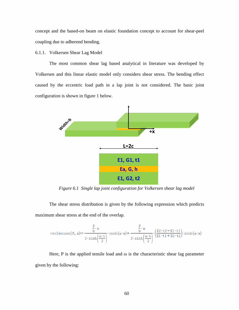
60
concept and the based-on beam on elastic foundation concept to account for shear-peel
coupling due to adherend bending.
6.1.1. Volkersen Shear Lag Model
The most common shear lag based analytical in literature was developed by
Volkersen and this linear elastic model only considers shear stress. The bending effect
caused by the eccentric load path in a lap joint is not considered. The basic joint
configuration is shown in figure 1 below.
Figure 6.1 Single lap joint configuration for Volkersen shear lag model
The shear stress distribution is given by the following expression which predicts
maximum shear stress at the end of the overlap.
Here, P is the applied tensile load and is the characteristic shear lag parameter
given by the following:

61
Although the joint ends should be stress free, the maximum values at the end should
be interpreted as stress at a point just near the edge. Some researchers have treated it as
average stress criteria by averaging over a distance equal to the adhesive thickness. TOM
modification to Volkersen involves a different shear lag parameter to include adherend
shear effect and implemented using a parameter () which depends on shear modulus of
adherend/adhesive. For =1, there is no adherend transverse shear effect on the shear stress
distribution.
For the ASTM 5868 configuration and properties of chosen material system (carbon
fiber reinforced epoxy laminate and epoxy adhesive), the adherend shear effect was found
to be quite negligible in Volkersen formulation.
6.1.2. Goland and Reissner (GR) Model
Goland and reissner model consider adherend bending effect due misaligned load
path of a single lap joint configuration as shown in figure 2.
For a lap joint with overlap length, 2c (L=2c) and adherend thickness t (t1=t2=t)
subjected to applied load, p per unit width (p=P/b), the shear stress distribution are given
by the following equations:

62
Figure 6.2 Single lap joint configuration for Goland and Reissner Shear-Peel
Coupling model
Here, k is the edge bending moment factor. TOM modification [4] again changes
to include adherend shear deformation effect defined by a parameter (). For the present
joint configuration, there is some adherend shear deformation effect and may be
considered. In TOM modification, k is very close to 1 and often taken as 1.
A plot of shear stress distribution with Volkersen, GR and GR-with TOM
modification is shown in figure 3. The lap shear strength data (24MPa) form manufacturer
has been used as failure criteria. There are significant ambiguity regarding proper failure

63
criteria. Without lack of custom experimental data on adhesive, it is not possible to apply
a different criterion at this time. However, the present approximation provides very
reasonable estimate. Experimental failure load was about 6049 N and the predictions look
very close from GR-Tom model.
Figure 6.3 maximum shear stress as a function of applied load for base joint
For weak interface, it is reasonable to assume that the adherend and adhesive do
not yield at all. Specifically, the adhesive act like a brittle manner and do not undergo
significant shear deformation due to lack of support from the weak adherend interface. We
postulate that once it tries to shear beyond linear strain limit, the weak interface fails before
allowing adhesive to shear. Hence, we take the linear strain limit of adhesive (about 0.0022)
as the failure criteria instead of shear strength in a strongly bonded joint. With 3.19GPa
adhesive modulus, this gives about 7MPa as the limiting stress level or failure criteria.
This choice of failure criteria is reasonable from another point of view. In chapter-
3, work of adhesion was calculated for modified and base laminate surface. The work of

64
adhesion for weak surface is about 3 times lower than that of base laminate. So reduction
of lap shear strength (failure criteria) by about a factor of 3 will yield 8 MPa which is close
to 7 MPa chosen as the failure criteria with approximate linear strain limit. The results are
plot in the following figures and intersections of failure criteria with max stresses are the
failure loads.
Figure 6.4 maximum shear stress as a function of applied load for weak interface
Table 6.1 Summary of Failure Load
Failure load, N
Joint
Type
Volkersen GR GR-
TOM
Experiment
ave
Base
lap joint
8850 5700 5100 6049
lap
joint-weak
interface
2575 1550 1475 2200
6.2. Dielectric Property Prediction Model for Bonded Joints
Dielectric properties of laminated joints depend on frequency dependent properties
of adherend and adhesive. It is understood that the joint will act as capacitor and hence

65
contribution from adhesive will dominate the low frequency response. Considering
electrode polarization constant in base joint and modified joint, the major polarization will
occur at material boundaries. Specifically, the adherend-adhesive interface polarization
will differentiate the base joint and the weak interface joint. The weak interface will have
a different polarization characteristic due to two major reasons: 1) chemical bonding is
different ii) roughness and wettability are different.
6.2.1 Impedance Model of Equivalent Joint
Considering above mechanisms, the objective here to develop a simplistic model
for predicting response of lap joint using adherend and adhesive properties. We will
present Impedance magnitude model first and future development will include complex
variable quantities (real and imaginary part isolation). The model does not include stray
capacity and line effects. Hence marginal difference in values are expected but the focus is
on capturing the trend.
The proposed model for equivalent impedance magnitude of the lap joint can be
written as:
Here, (f)= angular frequency, Zalow= impedance of adhesive at lower limit of
frequency (fmin), Zahigh= impedance of adhesive at higher limit of frequency (fmax), Z1
and Z2 are frequency-independent impedance of conductive carbon fiber/epoxy laminate.
It is to be noted that the Zalow and Zahigh data points will depend on adhesive thickness
(or volume fraction of adhesive).

66
For the weak joint, only one of the adherend-adhesive interface is modified. We
postulate that the polarization at this weak interface will change but will follow a similar
form of the low frequency contribution of adhesive to equivalent joint impedance. In
addition, the separation distance or thickness of adhesive will also affect this response of
modified interface. The weak interface will increase capacity and hence reduce impedance
of the system. In lap joint the impedance is mostly reactive although minimal resistive
contribution come from laminate only at higher frequency. Hence, we propose an empirical
form of equivalent joint impedance as follows and a better estimate of the interface effect
could be made in the future with full complex variable formulation.
Volume fraction of adhesive is defined as thickness ratios of adherend (t1 and t2)
and adhesive (ta):
6.2.2 Results of Equivalent Joint model and comparison with experimental data:
The figure below shows how impedance of undamaged base joint and joint with
weak interface varies with frequency (semi-log graph in figure 5).
If we look at the low frequency response at 0.1 Hz (figure 6), we can clearly observe
the effect of weak interface in the joint.

67
Figure 6.5 Comparison of experiment vs model estimate of impedance magnitude
Figure 6.6 Comparison of experiment vs model estimate of impedance magnitude

68
From the figure 5 and 6, it can be concluded that the empirical approximate model
captures the trend correctly. The exact magnitude is expected to be different as the idealized
equivalent model do not include circuit losses and exact polarization at adherend-adhesive
interface is not known. A future model of permittivity and sample capacity in the complex
function domain will be needed to quantify the exact interface effect but the validation
remains a change as probe can’t be placed at that interface unlike traditional electrode
polarization effect (4-probe setup).
6.3 Summary and conclusion
In this chapter, closed form analytical models have been applied to estimate failure
load in lap joint with weak interface. The brittle joint model based on shear lag is
determined to be best suited to capture the response. The failure criteria used is a simplistic
approximation but reasonable one as found to be consistent with work of adhesion studies.
More experimental data required to propose a failure criterion for weak interface. The
observed estimates of model and experimental data correlates very well.
Dielectric properties of lap joint have been estimated form adhesive and adherend
properties using empirical or approximate model. The estimated values differ from
experimental data but the trend is consistent. The benefit of such model is that parametric
studies can be performed to understand how adhesive thickness and other interface
properties may affect dielectric properties of the joint. More sophisticated models may be
developed in the future based on this fundamental understanding.

69
REFERENCES:
1. Budhe, S., et al. 2017. "An updated review of adhesively bonded joints in composite
materials," International Journal of Adhesion and Adhesives, 72: 30-42.
2. René Quispe Rodríguez, Paulo Sollero, Éder Lima de Albuquerque, STRESS
ANALYSIS AND FAILURE CRITERIA OF ADHESIVE BONDED SINGLE LAP
JOINTS. 21st International Congress of Mechanical Engineering October 24-28,
2011, Natal, RN, Brazil.
3. Charles Yang, John S. Tomblin, and Zhidong Guan. Analytical Modeling of ASTM
Lap Shear Adhesive Specimens. Report: DOT/FAA/AR-02/130
4. M. Y. Tsai, d. W, oplinger, j.morton. Improved theoretical solutions for adhesive lap
joints. lnt. J. Solids Struclures VoL 35, No. 12, pp. 1163-1l85, 1998.
5. Rene´ Quispe Rodrı´guez, William Portilho de Paiva, Paulo Sollero, Marcelo Ricardo
Bertoni Rodrigues, der Lima de Albuquerque. Failure criteria for adhesively bonded
joints. International Journal of Adhesion & Adhesives 37 (2012) 26–36.
6. Yarrington, P., C. Collier, and B. Bednarcyk, 2006, Failure Analysis of Adhesively
Bonded Composite Joints via the Virtual Crack Closure Technique, in 47th
AIAA/ASME/ASCE/AHS/ASC Structures, Structural Dynamics, and Materials
Conference. American Institute of Aeronautics and Astronautics.

70
CHAPTER 7
CONCLUSION AND FUTURE WORK
7.1 Summary of results and observations
Adhesive bonding of composite shows promising growth in a wide variety of
applications. In this work, we have shown that interfacial defects in composite joints can
be characterized by their dielectric properties. Broadband dielectric spectroscopy is shown
to be a valuable technique in capturing dielectric property changes. It has shown that the
dielectric response is most sensitive at low frequency, i.e. below 1 Hz. We have been able
to capture various type of surface modifications on composite laminate surfaces before and
after bonding. Unlike previous studies, we have proven that BbDS can be used to capture
the effect of defects at the interface of adhesive bond made of carbon fiber adherend.
Contact angle measurements are a proven method to check the wettability of bond
surfaces. Carbon fiber laminates under different type of surface modifications were used
to do wettability studies to imitate the possibility of impurities on adherend surface before
bonding. The change in dielectric properties due to those modification was then captured
by BbDS.
Overlap adhesive joints were made with several kinds of surface and volume
defects and tested for their dielectric properties. The results show that BbDS was able to
capture the change in dielectric properties based on the type of defect. Furthermore,
controlled specimens of single lap joint configurations were made with interfacial defect
to simulate weak bond with zero volume defect and tested for their bond strength by

71
loading until failure after testing for their dielectric properties. These dielectric
variables associated with weak bonds were assigned to specimens representing the
material’s state due to interfacial defects. The dielectric measurements are then related to
change in bond strength due to defects. The main advantage of this method is that it is
completely nondestructive because the applied voltage in BbDS is too low to cause any
harm to bond properties.
Analytical models were also used to investigate the estimated failure in lap joints
with weak interface and was found to be consistent with work of adhesion. An empirical
model was used to estimate that dielectric properties of lap joints are found to be matching
the trend of experimental data.
7.2 Potential future extension of work
The work in this thesis is ongoing and further study needs to be done by varying
thickness of specimen, measuring effect of different orientation of composite laminates,
different types of adhesive joints using broadband dielectric spectroscopy. More
sophisticated models needed to be developed by adding more experimental data to predict
weak interface.