Effect of Mesh Quality on Flux Reconstruction in …...FR is found to be more resilient to mesh...

Journal of Scientific Computing (2020) 82:77https://doi.org/10.1007/s10915-020-01184-2

Effect of Mesh Quality on Flux Reconstruction inMulti-dimensions

Will Trojak1 · Rob Watson2 · Ashley Scillitoe3 · Paul G. Tucker1

Received: 18 September 2018 / Revised: 19 November 2019 / Accepted: 30 December 2019 /Published online: 12 March 2020© The Author(s) 2020

AbstractTheoretical methods are developed to understand the effect of non-uniform grids on FluxReconstruction (FR) in multi-dimensions. A better theoretical understanding of the effectof wave angle and grid deformation is established. FR is shown to have a smaller variationin properties than some finite difference counterparts. Subsequent numerical experimentson the Taylor–Green Vortex with jittered elements show the effect of localised regions ofexpansion and contraction. The effect this had on Nodal DG-like schemes was to increasethe dissipation,whereas formore typical FR schemes the effectwas to increase the dispersion.Some comparison is made between second-order FR and a second-order finite volume (FV)scheme. FR is found to be more resilient to mesh deformation, however, FV is found to bemore resolved when operated at second order on the same mesh.

Keywords Flux reconstruction · Fourier analysis · Von Neumann analysis · Mesh quality ·Multiple dimensions

Mathematics Subject Classification 65M60 · 65T99 · 76F65 · 76M10

List of SymbolsRomana Convective velocity in xA Grid wave amplitudeb Convective velocity in yc(k) Wavespeed at wavenumber kC0ξ Centre cell FR matrix in ξ

C0η Centre cell FR matrix in η

CL Left cell FR matrix

B Will [email protected]

1 Department of Engineering, University of Cambridge, Cambridge CB2 1PZ, UK

2 School of Mechanical and Aerospace Engineering, Queen’s University Belfast, Belfast BT9 5AH,UK

3 Alan Turing Institute, Kings Cross, London NW1 2DB, UK

123

http://crossmark.crossref.org/dialog/?doi=10.1007/s10915-020-01184-2&domain=pdf

http://orcid.org/0000-0002-4407-8956

77 of 36 Journal of Scientific Computing (2020) 82 :77

CR Right cell FR matrixCB Bottom cell FR matrixCT Top cell FR matrixDξ ξ first derivative matrixDη η first derivative matrixEk Turbulent kinetic energyhL and hR Left and right correction functionshB and hT Bottom and top correction functionsknq Solution point Nyquist wavenumber, (p + 1)/δ jk knq normalised wavenumber, [0, π ]lk kth Lagrange polynomialp Solution polynomial orderqh Element shape factorQ Spatial scheme matrixR Update matrixu Primitive in real domain

Greekγ Grid geometric expansion factorδ j Mesh spacingη 2nd computational dimension variableε Enstrophyι VCJH scheme correction function variableι+ Variable ι for peak temporal stabilityκ(A) Condition number of matrix Aξ 1st computational dimension variableρ(A) Spectral radius of matrix Aτ Time stepΩΩΩ Solution domainΩΩΩn nth solution sub-domainΩΩΩ Standardised sub-domain

Subscript•B Variable at bottom of cell•L Variable at left of cell•R Variable at right of cell•T Variable at top of cellmax Maximum valuemin Minimum value

Superscript•T Transpose•δ Local polynomial fit of value•δC Correction to value•δD Localised discontinuous polynomial fit of value•δ I Common interface value based on local polynomial fit of value• Transformed variable• Locally fitted polynomial of variable

123

Journal of Scientific Computing (2020) 82 :77 of 36 77

Other∇ Gradient operator in computational domain�(z) Imagine part of z given z ∈ C

�(z) Real part of z given z ∈ C

C Set of complex numberR Set of real numbers

1 Introduction

Since the inception of the discontinuous spectral element methods of Quarteroni [34], stag-gered grid methods of Kopriva and Kolias [28], and spectral volume methods of Wang[56], the trajectory of high order methods has trended towards the Flux Reconstruction (FR)method of Huynh [24] and Vincent et al. [52]. This approach draws on the work of FiniteElements, (see Brenner and Ridgway-Scott [10]), enabling the high performance of FluxReconstruction on heterogeneous computing—as can be seen in the highly efficient use ofvast computing resources by Vincent et al. [55]. However, the move towards high order wasnot born out of a need for more efficient use of modern HPC environments. For example,Brandvik and Pullan [9] showed that high throughput could be obtained using second orderFinite Volume (FV) methods. Instead, the main motivating factor has been the increaseduptake by industry of turbulence resolving methods, such as Large Eddy Simulation (LES),as this allows for far better exploration of flow physics and moves towards the long term goalof computational wind tunnels. The main feature of LES is the modelling of the very smallestscales of motion, which reduces the need for the extremely high resolution required for DirectNumerical Simulation (DNS). However, Chow and Moin [14] and Ghosal [21] showed that,for LES, the need to keep the truncation error small to enable the sensible use of sub-gridscale models meant that the grid requirements are still demanding. A move to higher orderwould mean that the scaling of the truncation error with grid spacing occurs with a higherexponent—thus lowering the grid requirements and decoupling the scaling of aliasing errorand truncation error. Hence, for wall resolved LES, calculations are often impractical unlessthe more benign mesh resolution requirements of high order methods are considered.

The analytical understanding of Flux Reconstruction has been explored to a large extent inthe work of Vincent et al. [53], Jameson et al. [27], and Castonguay et al. [13], where the sta-bility of linear advection, advection–diffusion, and non-linear problems has been presented.The key findings were the energy stability of FR on linear problems, and the condition forenergy stability on non-linear problems. In addition, by investigating the dispersion and dis-sipation characteristics of FR, the existence of superconvergence after temporal integrationand the corresponding CFL limits were found. This work was limited to one dimension—although still applicable, the investigation of the exact behaviour of FR in higher dimensionshas been limited, such as that ofWilliams and Jameson [58] and Sheshadri and Jameson [39].This work focused primarily on the proof of the Sobolev-type energy stability in 2D similarto that of Hesthaven and Warburton [23], alongside some numerical studies performed forvalidation.

The advantage of FR—that leads to high performance on heterogeneous and massivelyparallel architectures—is its unstructured and sub-domain nature. Unstructured grids alsoallow far more complex geometries to be considered, but the resulting meshes experiencedeformation, expansion, and contraction of the elements. We wish to characterise the per-formance of FR under these conditions, and so far the effect of linear mesh deformation on

123


FR has been considered in one dimension by Trojak et al. [45]. Therefore, we make use ofthe seminal work of Lele [31], in which the dispersion and dissipation of finite differencemethods were considered in both one and two dimensions. We wish to repeat this processfor FR, and then extend it to also consider deformed grids.

In this paper, we present an extension to the one-dimensional analytical work of Vin-cent et al. [53] and Trojak et al. [45]. This extension will be shown for a two-dimensionalcase on quadrilaterals with rectilinear mesh stretching, but could also be performed on higherdimensional hypercubes. From the basis of this more general von Neumann analysis, thebehaviour of FR on linearly mapped meshes can be explored. The investigation has beenrestricted to linear transformations as these are of key importance for complex industrialsimulations due to their fundamental nature. For example, they occur in meshes where auto-mated mesh generators have simply tessellated elements to fill the domain. Understandingtheir character is key, however, we should point to some recent work that has numericallyinvestigated curved meshes [32,59].

The aim of this work is to understand the effect of moving to higher dimensionality onkey metrics governing scheme performance, such as CFL limit, dispersion, and dissipation.Finally, the Taylor–Green vortex will be used to understand how deformed meshes affect fullNavier–Stokes calculations, with reference calculations performed by an industrial secondorder finite volume method.

2 Flux Reconstruction

Flux Reconstruction [12,24] applied to the linear advection equation will form the basis ofthe initial investigation to be carried out, and for the reader’s convenience, an overview ofthe scheme is presented here. For a more detailed understanding, the reader should consultHuynh [24] or Castonguay [12]. The 1D scheme presented can be readily converted to twoand three dimensions for quadrilaterals and hexahedrals, respectively. First, let us considerthe one-dimensional advection equation:

∂u

∂t+ ∂ f

∂x= 0 (1)

The FR method is related to the staggered grid approach of Kopriva and Kolias [28] andDiscontinuous Galerkin (DG) [35], and as such it makes use of the same subdivision of thedomain into discontinuous sub-domains:

� =N⋃

n=1

�n (2)

Within the standardised sub-domain, � ∈ Rd , computational spatial variables are defined.

When d = 1, � = [−1, 1], using ξ to denote the value taken. This computational space isdiscretised with (p + 1)d solution points, and 2d(p + 1)d−1 flux points, placed at the edgesof the sub-domain. The solution and flux point locations are typically determined using atensor grid of a 1D quadrature. Figure 1a shows a 1D example of this. To transform from�n → �, a Jacobian Jn is defined such that:

uδ = uδ(ξ ; t) = Jnuδ(x; t) (3)

With this domain set up, we now proceed with defining the steps to construct a continuousflux polynomial from the discontinuous segments. The first stage is to define a local solution

123


(a) (b)

Fig. 1 Point layout in � for p = 3 and cell interface topology

polynomial in � using Lagrange interpolation.

lk(ξ) =p∏

i=0,i �=k

ξ − ξi

ξk − ξi(4)

uδ(ξ) =p∑

i=0

uδi li (ξ) (5)

Repeating the interpolation for the discontinuous flux in �:

f δD = f δD(ξ, t) =p∑

i=0

f δDi li (ξ) (6)

Here we define f δD as the transformed discontinuous flux polynomial. Now using the Jaco-bian and the solution polynomials, the primitive values can be calculated in the physicaldomain �n :

uδ(x) = uδ(ξ)

Jn=

p∑

i=0

uδi li (ξ) (7)

The primitive polynomial can then be interpolated to the interface and defined as uδl =

uδ(−1) and uδr = uδ(1). The values at the interface, I , then allow for a common interface

flux, f δ II , to be calculated in the physical domain. This is shown graphically in Fig. 1b.

For a general case, this is done using an approximate Riemann solver on the primitives atthe interface, such as: Roe [36]; flux vector splitting [49]; or HLL [22]. In order to get aspatially continuous flux over �, the common interface flux has to be incorporated into theflux polynomial interior of the element. For FR this is done by using a correction functionto propagate the corrected flux into �n . The exact definition of the correction function wasshown to be important in the determination of the characteristics of FR, by Vincent et al. [53].Primarily, the correction function is a polynomial which, in one dimension, has the boundaryconditions:

hL(−1) = hR(1) = 1 (8)

hR(−1) = hL(1) = 0 (9)

123


Beyond this, several sets of stable correction functions have been defined, firstly unifiedby Vincent et al. [52] and later expanded [43,44,48,54]. However, in this paper we will focuson the correction functions defined by Huynh [24], in particular the Huynh g2 correctionfunction, which is shown in Fig. 1a. We will also consider the correction that can recoverNodal Discontinuous Galerkin (NDG) [23] as it provides a good point of comparison, dueto the wide use and maturity of DG. It should be noted that the NDG correction functionwill only recover NDG in FR for homogeneous linear flux functions, due to the differentmechanisms of aliasing.

The correction to the flux function is then calculated using the difference between thediscontinuous and common interface values and a correction function. The correction isdefined as:

f δC =(f δ IL − f δD

L

)hL(ξ) +

(f δ IR − f δD

R

)hR(ξ) (10)

and hence the corrected continuous gradient of the flux is then:

∂ f δ

∂ξ= d f δD

dξ+ d f δC

dξ(11)

=p∑

j=0

f δDj

dl j (ξ)

dξ+

(f δ IL − f δD

L

) dhL(ξ)

dξ+

(f δ IR − f δD

R

) dhR(ξ)

dξ(12)

Finally, the solution is advanced in time following Eq. (13)—this can be performed via asensible choice of temporal integration.

∂ uδ

∂t= −∂ f δ

∂ξ(13)

Themethod detailed herewas shown in one dimension for simplicity, but thiswill be extendedto higher dimensionality in subsequent sections. We will briefly state here that, to increasethe dimensionality of the method, a tensor product is used. This is the samemethod as is usedin the analysis as well as in the formal implementation of a solver for hypercube elements.

3 Two-Dimensional von Neumann Analysis

The procedure for investigating the dispersion and dissipation properties of finite elementmethods has been laid out in some detail by Huynh [24], Hesthaven andWarburton [23], andVincent et al. [53]. It is broadly classified as a von Neumann analysis. The procedure was,however, mainly performed in 1D, with critical insight into the analytical performance ofFR when applied to more realistic problems overlooked. Extension of the analysis to higherdimension domains was performed by Lele [31] for various finite difference schemes. Thisdid, however, avoid the increased complexity of finite element von Neumann analysis. Tobegin our extension we introduce the 2D linear advection equation:

∂u

∂t+ ∇ · F = 0 (14)

F =[fg

]= ua =

[aubu

](15)

123


Flux reconstruction then uses the superposition of the discontinuous flux divergence and fluxdivergence correction, meaning Eq. (15) can be rewritten as:

∂ui, j∂t

= −∇ · FδDi, j − ∇ · FδC

i, j (16)

Taking the following definition of the Jacobian, the computational-physical domain transfor-mation can be defined:

G =[

∂x∂ξ

∂ y∂ξ

∂x∂η

∂ y∂η

]=

[G1 G2

G3 G4

]and J = |G| (17)

u = J−1u, F = J−1GF, ∇ · F = J−1∇ · F (18)

where we use ∇ to mean [ ∂∂ξ

, ∂∂η

]T in 2D. We will then impose that grid transformations arepurely rectilinear, i.e. G2 = G3 = 0. This is to reduce the number of dependent variables,while still allowing an important form of grid deformation to be investigated. From thework of Huynh [24], Castonguay [12], and Sheshadri et al. [40], Eq. (15) is written in twodimensions as:

∇ · FδD =p∑

i=0

p∑

j=0

f δDi, j

dli (ξ)

dξl j (η) +

p∑

i=0

p∑

j=0

gδDi, j

dl j (η)

dηli (ξ) (19)

∇ · FδC =p∑

i=0

((f δ IL,i − f δD

L,i

)dhL,i

dξ+

(f δ IR,i − f δD

R,i

)dhR,i

dξ

+(gδ IB,i − gδD

B,i

)dhB,i

dη+

(gδ IT ,i − gδD

T ,i

)dhT ,i

dη

)(20)

where we use L , R, B, and T subscripts to mean left, right, bottom, and top respectively. Wemay now use Eq. (19) and convert it into a matrix form:

∇ · FδD = Dξ fδ

i, j + Dη gδi, j (21)

∇ · FδD = G−11,i, jDξ f δ

i, j + G−14,i, jDηgδ

i, j (22)

To apply the correction function, we need to calculate the interface values around the element.For the case of generalised central/upwinding with upwinding ratio α, the common interfacefluxes may be written as:

G−14,i, j f

δ IL = a

(αG−1

4,i−1, j uδi−1, j,R + (1 − α)G−1

4,i, j uδi, j,L

)(23)

G−14,i, j f

δ IR = a

(αG−1

4,i, j uδi, j,R + (1 − α)G−1

4,i+1, j uδi+1, j,L

)(24)

G−11,i, j g

δ IB = b

(αG−1

1,i, j−1uδi, j−1,T + (1 − α)G−1

1,i, j uδi, j,B

)(25)

G−11,i, j g

δ IT = b

(αG−1

1,i, j uδi, j,T + (1 − α)G−1

1,i, j+1uδi, j+1,B

)(26)

where α = 1 gives rise to upwinding and α = 0.5 produces central difference. Hence, thedivergence correction can be written as:

∇ · FδCi, j = aα

G−14,i, j

(G−1

4,i−1, jhLlRT uδ

i−1, j − G−14,i, jhLlL

T uδi, j

)

+ a(1 − α)

G−14,i, j

(G−1

4,i+1, jhRlLT uδ

i+1, j − G−14,i, jhRlR

T uδi, j

)

123


(a)(b)

Fig. 2 Linear advection schematic for two and three dimensions

+ bα

G−11,i, j

(G−1

1,i, j−1hBlTT uδ

i, j−1 − G−11,i, jhBlB

T uδi, j

)

+ b(1 − α)

G−11,i, j

(G−1

1,i, j+1hTlBT uδ

i, j+1 − G−11,i, jhTlT

T uδi, j

)(27)

where hL now represents the gradient of the left correction function at the solution pointsand again lL are the values of the polynomial basis at the left interface and so on for R, T ,and B. Therefore, by grouping terms by their cell indexing and transforming each term intothe physical domain:

∂ui, j∂t

= − aG−11,i, j

(CLuδ

i−1, j + C0ξuδi, j + CRuδ

i+1, j

)

− bG−14,i, j

(CBuδ

i, j−1 + C0ηuδi, j + CT uδ

i, j+1

) (28)

where

CL = αhLlTR CR = (1 − α)hRlTL C0ξ = Dξ − αhLlT+ − (1 − α)hRlTR (29)

CB = αhBlTT CT = (1 − α)hTlTB C0η = Dη − αhBlTB − (1 − α)hTlTT (30)

Finally, as we are interested in the frequency response of the system, and, importantly toengineers and technicians, how the cell’s orientation relative to an oncoming wave affectsperformance. Therefore, we impose a trial solution of the form:

u(x, y; t) = exp (ik(x cos θ + y sin θ − ct)) (31)

and by substitution into Eq. (15), the advection velocity, a, can be found, which is shownschematically in Fig. 2a.

a =[ab

]=

[cos θ

sin θ

](32)

The plane wave can then be projected into the computational domain and discretised as:

ui, j = v exp(ik

((0.5(ξ + 1)δi + xi

)cos θ + (

0.5(η + 1)δ j + y j)sin θ − ct

))(33)

123


where, for brevity, δi = xi − xi−1 and δ j = y j − y j−1 are defined. Inserting Eq. (33) intoEq. (28), an eigenvalue problem can be obtained as:

−ikc(k)v = −G−11,i, j cos θ

(CL exp

( − ikδi−1 cos θ) + C0ξ + CR exp

(ikδi cos θ

))v

− G−14,i, j sin θ

(CB exp

( − ikδ j−1 sin θ) + C0η + CT exp

(ikδ j sin θ

))v

(34)

where �k(c(k)) = �(ω) and �(kc(k)) = �(ω) are the dispersion and dissipation, respec-tively, and ω is the modified angular frequency response of the system. By studying the trialsolution of Eq. (31) it can be understood that if �(ω) > 0 then the amplitude of the wave willincrease and vice versa. Furthermore, if�(ω) �= k then a wave will move at a different speedcompared to the other waves inside the packet. This causes the quality of the interpolation tobe affected as the solution is advanced in time. An important point is the difference betweenphase velocity ω/k and group velocity dω/dk. Phase velocity is the speed of a wave in apacket of waves. Group velocity is the speed of the packet. Therefore, changes to dω/dk canbe thought of as changes to the physics due to the numerical method.

Equation (34) can alternatively be cast in the form of an update equation. If initiallyEq. (28) is combined with Eq. (33), then a new matrix, Qi, j , can be defined:

∂ui, j∂t

= Qi, jui, j (35)

Qi, j = −G−11,i, j cos θ

(CL exp

( − ikδi−1 cos θ) + C0ξ + CR exp

(ikδi cos θ

))

− G−14,i, j sin θ

(CB exp

( − ikδ j−1 sin θ) + C0η + CT exp

(ikδ j sin θ

))(36)

This definition of the semi-discrete FR operator, Q, can then be used to form what is calledthe update equation by imposing some temporal discretisation. As such we may write:

un+1i, j = R(Qi, j )uni, j (37)

R33 = I + τQi, j

1! + (τQi, j )2

2! + (τQi, j )3

3! (38)

where the superscript denotes the time level, and our update matrix is R. Shown here is alsoan example definition for R for a 3-step 3rd-order Runge–Kutta time integration scheme.Finally, in keeping with von Neumann’s theorems [25,30] and Banach’s fixed point theorem[29], the spectral radius ofR has to be less than or equal to 1 for stability. ρ(R) � 1∀ k ∈ R.

In recent works by Vermeire et al. [51] and Trojak et al. [46], the Fourier analysis wasextended by fully discretising the equation. This is performed by taking Eq. (37) and againapplying Eq. (31). This results in:

exp (−ik(c − 1)τ )v = λv = exp (ikτ)R(k, τ )v (39)

where the time step from n to n + 1 is τ . Hence, we rearrange for the modified wave speed:

c = i log (λ)

kτ+ 1 (40)

where λ are the eigenvalues of exp (ikτ)R. The advantage of this further analysis is that itgives the dispersion and dissipation relations of the full scheme as would be experiencedwhen applied as implicit LES.

123


The results of this section can then be extended to n-dimensions. The analysis can broadlybe repeated but is beyond the scope of this work. But, we give the example for 3D Blochwave as:

u = exp(ik(x cosφ cos θ + y cosφ sin θ + z sin φ − ct)

)(41)

where the angles are as shown in Fig. 2b, and hence the 3D convective velocities for linearadvection are:

a =⎡

⎣cosφ cos θ

cosφ sin θ

sin φ

⎤

⎦ (42)

4 Two-Dimensional Error and Convergence Analysis

The techniques applied to the linear advection equation of Sect. 3 can be further extendedto examine the effects of the grid and wave angle upon the error convergence. This methodwas initially presented for a 1D uniform grid in FR by Astana et al. [4], and for fully-discreteequations by Trojak et al. [46]. Here we will extend the analysis to include stretched grids intwo dimensions with (p+1)2 solution points. To begin, we will diagonalise the semi-discreteFR operator matrix as:

Q = W�W−1 = Wik�W−1 (43)

Here W is an eigenvector matrix and � is the diagonal eigenvalue matrix. The matrix � isthen a normalised form of the eigenvalue matrix, used to simplify later notation. This diago-nalisation may then be exponentially integrated in order to advance the solution continuouslyin time such that:

uδi, j (t) = exp (ctQ)u(0) = W exp (ikct�)W−1u j (0) (44)

Here the definition of a matrix exponential has been used with W−1W = I to simplify theform. The initial condition is then required and is defined as:

ui, j (0) = exp (ik(x j cos (θ) + y j sin (θ))Wβββ (45)

For convenience we will define the solution shift based on the cell location as:

uc,i, j = exp(ik(xi cos (θ) + y j sin (θ)

)(46)

The initial condition may then be substituted into Eq. (44), leading to:

uδi, j (t) = uc,i, jW exp (−ikct�)βββ = uc,i, j

(p+1)2∑

n=1

exp (−ikctλn)βnwn (47)

Here wn is the nth eigenvector taken from W and βn is the nth coefficient taken from βββ.The semi-discrete error may then be calculated by analytically evolving the discrete solutionusing exponential integration. Hence, the analytical solution in time is:

ui, j (t) = uc,i, j exp (−ikct)ui, j (0) = uc,i, j exp (−ikct)(p+1)2∑

n=1

βnwQ,n (48)

123


Therefore, the semi-discrete error can be formed by subtracting Eq. (48) from Eq. (47) as:

ei, j (t, k) = uδi, j (t, k) − ui, j (t, k)

= uc,i, j exp (−ikct)(p+1)2∑

n=1

(exp

(ikct(λn + 1)

) − 1)βnwQ,n

(49)

This measure of the semi-discrete error can then inform how the error changes with gridandwavenumber, some results ofwhichwere investigated for 1DNDGvia FRbyAstana et al.[4]. Subsequently, the error may form a rate of convergence, which for grid spacing is then:

rh(t, k) = log (‖ei, j (t, k, J1))‖2) − log (‖ei, j (t, k, J2))‖2)log (J1) − log (J2)

(50)

Here J1 and J2 are the Jacobians for two different grid spacings. The rate of convergencewith wavenumber is similarly defined as:

rk(t, J ) = log (‖ei, j (t, k1, J ))‖2) − log (‖ei, j (t, k1, J ))‖2)log (k1) − log (k2)

. (51)

5 Analytical Findings

The analytical methods presented in Sects. 3 and 4 allow us to investigate many properties ofFR, however from Eqs. (36–38) it can be seen that the functional space ofQ is 8 dimensional,leading to the functional space of ρ(R) being 9 dimensional (τ, γx , γy,Δx ,Δy, k, θ, ι, p).Therefore, we need to restrict our investigation to some key results relating to grid deforma-tion. Firstly, understanding the dispersion and dissipation (�(ω) and �(ω)) in 2D for bothuniform and stretched grids will be important. Secondly, we wish to briefly understand howhigher dimensionality and grid deformations affect the temporal stability of FR through eval-uation of the CFL limits [16]. Then we will go on to study the effect of grid deformation andincident angle on the rate of convergence.Wewill finish the analytic studywith the evaluationof the fully-discrete dispersion and dissipation relations. Throughout this investigation wewill also look to understand the effect of the correction functions on these properties.

5.1 Review of 1D Grid Expansion

Before commencing with the Fourier/von Neumann analysis in 2D, we will give a briefreview of the behaviour exhibited in one dimension. Figure 3 shows the results for upwindedNDG correction functions at various order.

The results are separated into the real and imaginary parts of ω, where they representdispersion and dissipation respectively. Ideally �(ω) = 1 and �(ω) = 0. However, thenumerical discretisation will cause deviation from the ideal dispersion, while the interfaceupwinding here will cause dissipation. In [47] a non-conservative Jacobian definition wasused that resulted in variation of the numerical characteristics as the grid was deformed.However, if a conservative Jacobian is properly applied, then grid stretching has no impactupon dispersion and dissipation of FR other than a change in the Nyquist wavenumber. Fora geometrically deformed grid the Nyquist wavenumber will be:

knq = 1

2γ (p + 1)(52)

123


(a) (b)

Fig. 3 Upwinded 1D FR, for various orders with NDG correction functions

This raises the question, of what is the impact—for this linear system in 2D—of stretching thegrid in x and y? And what implications will these effects have for the practical application ofthe scheme?Additionally, what implications will any effects have on the practical applicationof the scheme?

5.2 Effect of Grid on Dispersion and Dissipation

For the higher dimensional case, we begin by considering the dispersion and dissipationon a uniform grid in two dimensions as order is varied. We are concerned here with theprimary mode—as FR has multiple modes, this is the one that physically represents the wave.Although, as was found by Asthana et al. [4], this may not be how the energy distributesitself. We identify the physical mode as that which has the largest contribution to the energyat very low, well resolved, wavenumbers.

For this investigation into the dispersion and dissipation characteristics of FR, we wishto make a note of the Nyquist frequency of the elements. The Nyquist frequency has adependency on the expansion ratio. This is found from the harmonic mean of the 1D Nyquistfrequencies, then normalised by the adjacent element size at that angle. Hence, the normalisedwavenumber is then:

k = k/knq = 1

2kmax

{cos (θ), sin (θ)

}( 1

p + 1

)√(cos (θ)

γx

)2

+(sin (θ)

γy

)2

(53)

The dispersion and dissipation relations are then shown in Figs. 4 and 5 . It is clear thatfor all orders FR becomes dispersive as the incidence angle is increased to θ = 45◦, but thenreturns to a dispersion similar to that of θ = 0◦ close to θ = 45◦. This can be seen by thebowing out of the contour as the angle approaches 45◦ before receding at θ = 45◦. In thecase of dissipation for uniform grids, the dissipation decreases as the angle increases towardsa minimum at θ ≈ 30◦. Once again at θ = 45◦, the dissipation returns to that of a wave at 0◦.This behaviour, where both the dispersion and dissipation at θ = 0◦ and 45◦ are the same, isdue to the projection of the wave in y being zero in the θ = 0◦ case and the projections in xand y being the same in the θ = 45◦ case.

Looking at the trends shown as order is varied, order seems to only have aminor impact onthe angular spread over which the dispersion and dissipation changes. By comparison withthe results of Lele [31], where a similar test is performed for finite and compact difference

123


(a) p = 2. (b) p = 3.

(c) p = 4. (d) p = 5.

Fig. 4 Primarymodedispersion for 2DupwindedFR,withHuynh g2 corrections, at various orders.Normalisedwavenumber as radial distance (markers atπ/4 intervals), and element angle of incidence as azimuthal distance

schemes, FR shows a comparatively smaller change in performance as the angle is varied. Itis thought that this is due to the method of polynomial fitting used by FR, namely that thisimplementation of FR used a tensor grid of monomials i.e., the number of solution pointsis (p + 1)d and hence the monomials in the interpolation go from (ξ0η0, ξ1η0 . . . ξ pηp).By contrast, finite differences do not include the cross product terms, which will becomeincreasingly dominant as the angle is increased.

123


(a) (b)

(d)(c)

Fig. 5 Primary mode dissipation for 2D upwinded FR, with Huynh g2 corrections, at various orders. Nor-malised wavenumber as radial distance (markers atπ/4 intervals), and element angle of incidence as azimuthaldistance

Moving on, we then consider the impact of non-uniform grids on the character of the dis-persion and dissipation. In particular, we explore the effect of grid expansion and contractionand how they interact, if there is expansion orthogonal to contraction. Initially we will focuson Huynh’s g2 correction function, the results of which are summmarised in Fig. 6.

Let us first focus on the case of γx = 1 and γy = 1.1, as is presented in Fig. 6a, b. Inthe region of 0◦ < θ < 45◦, the impact of the perpendicular grid expansion has been toreduce �(ω)—most notably near θ = 45◦—as is exemplified in Fig. 7a. Conversely, in the

123


(a) Dispersion, γx = 1, γy = 1.1. (b) Dissipation, γx = 1, γy = 1.1.

(c) Dispersion, γx = 0.9, γy =1.1.

(d) Dissipation, γx = 0.9, γy =1.1.

Fig. 6 Two dimensional upwinded FR, p = 3 with Huynh g2 corrections, for different grid expansion factors.Normalised wavenumber as radial distance (markers at π/4 intervals), and element angle of incidence asazimuthal distance

range 45◦ < θ < 90◦ the grid expansion has caused an increase in dispersion. For the caseof p = 3 explored here, this action is beneficial, however, as order is increased further thismay cause a detrimental dispersion overshoot to develop. Studying the impact on dissipationfor γx = 1, γy = 1.1 case, associated with the increase in dispersion, there is additionaldissipation over the central wavenumbers. This is preceded by a reduction in dissipation nearthe Nyquist wavenumber. This behaviour is reversed for dissipation in 45◦ < θ < 90◦.

123


(a) Dispersion. (b) Dissipation.

Fig. 7 Two dimensional upwinded FR, p = 3, with Huynh g2 corrections at selected incident angles andstretching

We may now apply a contraction perpendicular to an expansion, shown in Fig. 6c, d.The trends that were discussed for γx = 1, γy = 1.1 seem to continue when an additionalcontraction is applied. However, the contraction has served to amplify the effect seen previ-ously, which is more clearly visible in Fig. 7. It should also be remarked that the dispersionand dissipation at θ = 45◦ is no longer the same as the θ = 0◦ case. This is due to theprojection into x and y no longer being the same, which can be understood from Eq. 53. Thisequation also indicates the origin of the differences with angle and deformation: that, afterprojection into x and y, the wave components will have different normalised wavenumbersin the element they are advecting from, and hence different properties.

To understand this further we can think about a given wave decomposed into x and ycomponents initially at θ = 45◦. For γx = 1 and γy = 1.1 we may calculate the normalisedwavenumber of the projections in the adjacent upwind elements, thiswill aid in understandinghow the incoming solution is affected. Although they should be equal, the projection in y willhave a lower wavenumber due to the smaller size of the element from which it is advecting.At lowwavenumbers this difference will have a small impact on the 2D result as in both x andy we have c ≈ 1. However at higher wavenumbers the effect will become more pronounced.Larger variations are then seen at other angles due to the projections, even for a uniform grid,having different wavenumbers and hence properties. This also explains why, in Fig. 7, wesee the effect of grid deformation being approximately symmetric about the uniform case.Furthermore, this explains why coupling an expansion and contraction causes the effect tobecome more pronounced.

We will now vary the correction function and investigate the effect of grid stretching.Here we will apply the NDG correction function, the results of which are presented in Fig. 8.When applied to a uniform grid, it is evident that NDG exhibits similar changes comparedto Huynh’s g2 as the incidence angle is varied. Nonetheless, the variation of dispersion anddissipation with θ appears to be smaller for NDG. As the grid is then deformed, the samechanges in the properties take place. Yet, due to the dispersion overshoot of NDG in theuniform case, stretching has led to the changes in dispersion becoming more significant.

123


(a) Dispersion, γx = γy = 1.0. (b) Dissipation, γx = γy = 1.0.

(c) Dispersion, γx = 0.9, γy =1.1.

(d) Dissipation, γx = 0.9, γy =1.1.

Fig. 8 Two dimensional upwinded FR, p = 3 with NDG corrections, for different grid expansion factors.Normalised wavenumber as radial distance (markers at π/4 intervals), and element angle of incidence asazimuthal distance

5.3 Effect of Grid on Error and Convergence

The dispersion and dissipation relations explored show that grid expansion, contraction andincidence angle can have an appreciable impact on the numerical characteristics of FR. Ameans of measuring the impact of these variations is through calculating analytically theerror of the method.

123


(a) Huynh g2. (b) NDG

Fig. 9 Semi-discrete error of FR, p = 3, with upwinded interfaces on a uniform grid for θ = 45◦

Beginningwith a uniformgrid, the errorwithwavenumber for a uniformgrid can be seen inFig. 9.Here, time has been normalised by thewave’s time period. Figure 9a shows thatwemayseparate the error into three regions. Low wavenumbers, where the well resolved waves havelow levels of error. High wavenumbers, where the lower dissipation of Huynh’s g2 correctionfunction leads to some high amplitude oscillations. Previous works [4,46] found that theseoscillations were due to the solution being formed from secondary, erroneous, modes. Lastly,there is a central range of wavenumbers where the solution is still mainly composed of theprimary mode, however, the primary mode’s dissipation is increasing. Therefore, waves herequickly become damped and the error grows.

Comparisonmaybemade to the error evolution forNDG, shown inFig. 9b. It is evident thatNDG has lower error and a wider range of wavenumbers over which waves are well resolved.At higher wavenumbers NDG also produces lower amplitude spurious waves. This is due tothe higher dissipation of NDG compared to g2. In the intermediate range of wavenumbers,transients in the error early on are visible for both NDG and g2. However they appear smallerfor NDG, again associated with the higher dissipation and reduced half-life of the spuriousmodes.

The error results presented here were for a wave at 45◦. To understand the effect ofincidence angle, the error calculated may then be used to produce a rate of convergencewith grid spacing via Eq. (50). A rate of convergence with wavenumber is similarly defined,Eq. (51). However, this givesmuch the same insight as rh and is left out for brevity. The resultsfor rh on a uniform grid, at an absolute wavenumber of k = 2 and J1/J2 = 2 are then shownin Fig. 10. For NDG, Fig. 10a, the initial rate of convergence is 4 and, after the dissipationof spurious modes, the rate can be seen to be increasing towards 7. This is the expectedbehaviour explored by Asthana et al. [4]. As the angle is varied, however, the time for thescheme to reach the convergence-rate-limit increases. This indicates that as the incidenceangle is increased towards θ = 45◦, the half-life of the secondary modes may also increase.This is rooted in the use of an anisotropic quadrature to form the polynomial approximation.In particular, we use a tensor grid, which has higher resolution on the diagonal. Hence,although the primary mode is unaffected at θ = 45◦, we have shown here that the resolutionof the secondary mode is increased. Consequently, this could mean that when the method isapplied practically, grid alignment could impact results.

123


(a) NDG. (b) Huynh’s g2.

Fig. 10 Grid spacing rate of convergence of FR, p = 3, with upwinded interfaces on a uniform grid

Fig. 11 Semi-discrete error ofFR, p = 3, upwinded interfaceswith: γx = 1, γy = 1.1, andθ = 30◦. Here Huynh’s g2correction function has beenapplied

Again, investigating the effect of changing to Huynh’s g2 correction function (Fig. 10b)we see that the initial rate is the expected value of 4, which then asymptotes to a value of6. The decrease relative to NDG is due to the well know super-convergence of DG [3,15],and in FR is rooted in the g2 correction function having lower order, p − 1, terms. For g2correction functions, the reduction in the dissipation for θ ≈ 30◦ and θ ≈ 60◦ coincideswith an increase in the time to reach the convergence limit, similar to that observed for NDG.However, the g2 correction functions goes on to have a slight increase in the convergence limitaround θ = 45◦. In a more general sense, it may be remarked that g2 correction functionsmay be more resilient in higher dimensions due to smaller variation in properties that thisrate investigation shows.

Now applying a grid expansion in the y direction, we obtain the error results presentedin Fig. 11. Here we have extended the time window of the analysis to demonstrate a keyresult. For the range of wavenumbers that would be expected to be well resolved, the errorsteadily increases with time. This is not due to excess dissipation. It is clear from Fig. 6bthe change in dissipation in this range is negligible, and is in fact reduced. Inspection of thevalues of � instead show there is a small reduction in the phase velocity (ω/k), which willhave an associated reduction in the group velocity (∂ω/∂k). Therefore, the speed at whichthe wave is propagating is incorrect and manifests itself as a gradually oscillating error. Dueto this behaviour of the error, it has not been possible to calculate the rate of convergence onstretched grids.

123


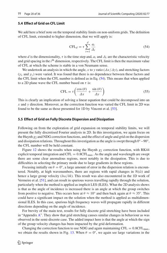
5.4 Effect of Grid on CFL Limit

We add here a brief note on the temporal stability limits on non-uniform grids. The definitionof CFL limit, extended to higher dimension, that we will apply is:

CFLd = τ

d∑

i=1

aiΔi

(54)

where d is the dimensionality, τ is the time step and, ai and Δi are the characteristic velocityand grid spacing in the i th dimension, respectively. The CFL limit is then the maximum valueof CFL at which the scheme is stable in a von Neumann sense.

We undertook an analysis in which the angle, x to y ratio (Δx/Δy), and stretching factors(γx and γy) were varied. It was found that there is no dependence between these factors andthe CFL limit when the CFL number is defined as in Eq. (54). This means that when appliedto a 2D plane wave the CFL number based on τ is:

CFL = τ

(cos (θ)

Δx+ sin (θ)

Δy

)(55)

This is clearly an implication of solving a linear equation that could be decomposed into anx and y direction. Moreover, as the correction function was varied the CFL limit in 2D wasfound to be the same as those presented for 1D by Vincent et al. [53].

5.5 Effect of Grid on Fully Discrete Dispersion and Dissipation

Following on from the exploration of grid expansion on temporal stability limits, we willpresent the fully discretised Fourier analysis in 2D. In this investigation, we again focus ontheHuynh g2 andNDGcorrection functions, and the effect of angle and grid on the dispersionand dissipation relations. Throughout this investigation as the angle is swept through 0◦−90◦,the CFL number will be held constant.

Figure 12 shows the results when using the Huynh g2 correction function, with RK44explicit temporal integration and CFL = 0.8CFLmax. As the angle and wavelength are sweptthere are some clear anomalous regions, most notably in the dissipation. This is due todifficulties in selecting the primary mode due to large gradients in these regions.

Focusing initially on θ = 0◦, a large amount of error in the dispersion relation is encoun-tered. Notably, at high wavenumbers, there are regions with rapid changes in �(ω) andhence a large group velocity (∂ω/∂k). This result was also encountered in the 1D work ofVermeire et al. [51], and can result in spurious waves travelling rapidly through the solution,particularly when the method is applied as implicit LES (ILES). What the 2D analysis showsis that as the angle of incidence is increased there is an angle at which the group switchesfrom positive to negative. This occurs here at θ ≈ 10◦ and then back again at θ ≈ 35◦. Thiscould have a significant impact on the solution when the method is applied as multidimen-sional ILES. In this case, spurious high frequency waves will propagate rapidly in differentdirections depending on the angle of incidence.

For brevity of the main text, results for fully discrete grid stretching have been includedin “Appendix A”. They show that grid stretching causes similar changes in behaviour as wasobserved in the semi-discrete case. The added impact here is that the angle at which the signof the group velocity changes has been impacted by the grid deformation.

Changing the correction function to use NDG and again maintaining CFL = 0.8CFLmax,we obtain the results shown in Fig. 13. When θ = 0◦, we again see large variations in the

123


(a) Dispersion: γx = γy = 1. (b) Dissipation: γx = γy = 1.

Fig. 12 Dispersion and dissipation of upwindedFR, p = 3,withHuynh g2 corrections, explicit RK44 temporalintegration, and CFL = 0.8CFLmax. The radial distance is the normalised wavenumber (including the effectof angle), and the azimuthal distance is the angle of incidence to the element

(a) Dispersion: γx = γy = 1. (b) Dissipation: γx = γy = 1.

Fig. 13 Dispersion and dissipation of upwinded FR, p = 3, with NDG corrections, explicit RK44 temporalintegration, and CFL = 0.8CFLmax. The radial distance is the normalised wavenumber (including the effectof angle), and the azimuthal distance is the angle of incidence to the element

123


dispersion. However, for NDG at highwavenumbers, there is initially an increase in�(ω) fol-lowed by a sharp decrease. This will bring about very high values of group velocity. Sweepingthe incidence angle shows somewhat different behaviour to g2 correction functions. Thereis still a form of change that occurs at θ ≈ 10◦ and θ ≈ 35◦, but it has a different character.Now after the switch, the initial increase in dispersion is reduced, and, by inspection, thegroup velocity at the extreme end of the frequency range seems to have reduced. Throughoutthe range of wavenumbers with high group velocities, Fig. 13b shows that there is a largeamount of dissipation that may reduce the effect of the dispersion. Therefore, it seems thatthe NDG correction function for ILES with explicit temporal integration may cause smallerdispersion errors for waves that are not grid aligned.

Again, for brevity of the main text, results of grid deformation with the NDG correctionfunction are shown in Appendix A. They indicate the effect of grid deformation is to causea similar change as to that of the semi-discrete case.

6 Non-linear Navier–Stokes Equations with Deformed Grids

It is common within the CFD community to use the canonical Taylor–Green Vortex (TGV)[41] test case to assess the numerics of a solver applied to the Navier–Stokes equationswith turbulence—and to that end, there is a plethora of DNS data available for comparison[19,50]. However, this case is quite contrived and ultimately will favour spectral or structuredmethods due to the Cartesian and periodic domain, whilst also being unrepresentative ofengineering flows that are often wall bounded and/or have complex geometries. Hence, wepropose deforming the elements, initially linearly by jittering the corner nodes to be morerepresentative of real mesh conditions. Importantly, these deformations will introduce crossmultiplication into the Jacobian, as well as local regions of expansion and contraction.

The initial conditions of the TGV applied here are those of DeBonis [19], where thecharacter of the flow is controlled by the non-dimensional parameters defined as:

Re = ρ0U0L

μ, Pr = 0.71 = μγ R

κ(γ − 1), Ma = 0.08 = U0√

γ RT0(56)

where we will use the standard set of free-variables for the velocity, density, pressure, andgas characteristics:

U0 = 1, ρ0 = 1, p0 = 100, R = 1, γ = 1.4, L = 1 (57)

Here, due to the solver implementation, we use a specific gas constant of unity and hence,to achieve the required Reynolds and Prandtl numbers, the dynamic viscosity and thermalconductivity are set appropriately. The statistics that will be studied here are the decay of thekinetic energy and the enstrophy scaled by viscosity, which are defined respectively as:

−dEk

dt= − 1

2U 20 ρ0|�|

d

dt

∫

�

ρ(u2 + v2 + w2)dx (58)

ε = μ

U 20 ρ2

0 |�|∫

�

ρ(ωωω · ωωω)dx (59)

whereωωω = ∇ ×[u, v, w]T is vorticity and |�| is the domain volume. The enstrophy is scaledin such a manner as it is known that in the incompressible case enstrophy and kinetic energydissipation can be directly related this way. Throughout, a reference DNS solution—labelledref—is provided from van Rees et al. [50].

123


The FR method is extended to 3D hexahedrals—from 2D quadrilaterals—by the sametensor product formulation of Huynh [24]. The invisicid common interface calculation wasperformed using a Rusanov flux [37] with a Davis [17] wave speed. The viscous commoninterface calculation was the BR1method of Bassi and Rebay [5,6]. Here, the gradients of theC0 continuous solution is required at thefluxpoints. These are calculatedbyfirst correcting thegradient at the solution points, then interpolating this to the flux points. Fromhere the gradientcan be transformed from the computational space to the physical space. The alternative wouldbe to interpolate the solution point gradient after transforming it to the physical space. Thetwo methods will give different results on complex element transformations, however due tothe small scale of the viscous terms in the forthcoming cases, investigation of this differencewill be deferred.

6.1 Randomised Grids

As has been stated, we begin by taking a uniform periodicmesh on the domain� ∈ [−π, π]3,and jittering corner nodes of the elements that are interior to the domain. The degree of jitteris calculated using a time seeded random number shifted to be centred about zero and scaledby a global factor, j f , between zero and unity. The scaling factor is such that zero gives auniform mesh and unity could lead to edges of zero length. This transformation is definedas:

x ′ = x + j fl(x − 0.5)

nx(60a)

y′ = y + j fl(y − 0.5)

ny(60b)

z′ = z + j fl(z − 0.5)

nz(60c)

where x ′ etc. are the new points, x etc. are a uniform base grid, and x j ∈ (0, 1] etc. arerandom numbers. To assess the grid quality, we seek a single a metric to describe the relativequality of the meshes produced. We opted for a volume ratio shape factor, slightly redefinedas:

qh = 6√

πVh

S3/2h

(61)

where Sh is the surface area of the hexahedral element and Vh is its volume. The qualitymetric, qh , is then defined as the ratio of the volume of the element to the volume of a spherewith the same surface area, with qh = √

π/6 for a perfect cube. To put this parameter intocontext, some example meshes are shown in Fig. 14.

As part of the jittering process, only the four vertices of each element were moved. Itremains to propagate these distortions through to the solution and flux points required by theFlux Reconstruction approach. The distortions considered as part of this work were purelylinear, and thus the effect of jittering the element vertices could have been carried through tothe internal solution points and flux points by use of bilinear interpolation. However, with aview to future work in which non-linear distortions will be applied to the elements, a RadialBasis Function based approach was used to perform the interpolation.

Radial Basis Functions are well known in computational physics for mesh distortion andgeneralised interpolation (see, for example, [7,11,18]). They allow for the easy and smoothinterpolation of scattered data, and, in this specific case, for the interpolation of volume

123


(a) qh =√

π/6 ≈ 0.7236. (b) qh = 0.7201. (c) qh = 0.7016.

Fig. 14 Example slices through a 3D hexahedral mesh to illustrate the mesh quality metric

(a) Selected turbulent kinetic energy dissi-pation.

(b) Variation of turbulent kinetic energy dis-sipation with jitter. Dashed contour at zerodissipation.

Fig. 15 Effect of jitter on turbulent kinetic energy dissipation of the TGV (Re = 1600) for FR, p = 2, withHuynh g2 correction functions on a 1203 DoF mesh. Explicit time step size is Δt = 1 × 10−3

distortion from prescribed boundary distortions. A wider discussion of the use of RBFs isoutside the scope of this paper, but they take the general form:

f (x) =n∑

i=1

λiφ (||x − xi ||) (62)

where λi are weights, and φ is the basis function. The thin plate spline is a widely used radialbasis function for mesh warping, and is defined as [20]:

φT PS = ||x − xi ||2 ln ||x − xi || (63)

Once the vertex distortion has been propagated through the solution and flux points of thecell, the Jacobian of the transformation can be defined. Initially, this will be done using thenon-conservative formulation (ξx = yηxζ − yζ xη). This might be expected to be sufficientfor the linear distortions to the elements which are being applied here.

Figures 15 and 16 show the first of these results. First looking at Figs. 15a and 16a, whichshow two specific dissipation curves for a uniform and jittered mesh. At the beginning of thesimulation, there is a clear time at which the global energy increases. Extending these runs tocovermultiple grid qualities, Figs. 15b and 16b, it is observed that as the grid quality decreasesa region where turbulent kinetic energy increases soon emerges. As time progresses, energydissipation is again seen and the point of peak dissipation arrives early, moving from t ≈ 8.5to t ≈ 7.5. The same behaviour is seen for both p = 2 and p = 4. From comparison of

123


(a) Selected turbulent kinetic energy dissi-pation.

(b) Variation of turbulent kinetic energy dis-sipation with jitter. Dashed contour at zerodissipation.

Fig. 16 Effect of jitter on turbulent kinetic energy dissipation of the TGV (Re = 1600) for FR, p = 4, withHuynh g2 correction functions on a 1203 DoF mesh. Explicit time step is Δt = 1 × 10−3

(a)p = 2. (b)p = 4.

Fig. 17 Comparison of TGV (Re = 1600) enstrophy for 1203 degree of freedom grid with similar qh

p = 2 and p = 4, it seems that p = 4 is slightly more robust to grid deformation, as p = 4was able to run at qh ≈ 0.7, whereas for p = 2, qh could not be reduced much below 0.717for 1203 DoF without completely diverging.

The explanation of this is believed to be due to two interacting components. The firstis that, although the randomised grid transformation applied here is linear, the thin platespline RBF method will not recover an exactly linear model of the transformation. Hence,the second factor is that the non-conservative method for defining the Jacobian is no longersufficient to accurately define what is now essentially a non-linear transformation. Remedialactions will be presented shortly.

Studying the effect of jittered grids on enstrophy, shown in Fig. 17, it is clear that as thegrid is stretched the enstrophy increases. This is indicative of an increase in the vorticity,with the rise occurring within t = 0 − 1. This is consistent with energy being added at thelarge scales, as at this time there are only large scales present. After the initial increase, theenstrophy returns to following the trend of the uniform case. However, in the case of p = 2,Fig. 17a, a larger initial increase is seen followed by a wider peak. The wider peak is similarin character to that of the uniform case and is due to the grid being mildly under-resolvedin the p = 2 case relative to the DNS. This aims to show that RBF grid transformation canresult in non-linearities in the grid and, when coupled to a non-conservative Jacobian, thismanifests itself in the energy of the largest scales increasing.

We will investigate further the effect of mesh jittering by instead using the symmetricconservative method similar to that of Thomas et al. [42] (ξx = [(yηz − zηy)ζ − (yζ z −zζ y)η]/2). Further to this we will also use the grid interpolation methodology of Abe [1].

123


(a) (b)

Fig. 18 Comparison of polynomial and RBF methods for point placement on jittered meshes. This is for aTGV, Re = 1600, p = 4, 1203 DoF, RK44, and Δt = 10−3. A jitter factor of j f = 0.3 and 0.2 givesqh = 0.7157 and 0.7199 respectively

(a) Kinetic energy dissipation. (b) Enstrophy based dissipation.

Fig. 19 Comparison of Huynh g2 correction functions with NDG for jittered meshes. This is for a TGV,Re = 1600, p = 4, 1203 DoF, RK44, and Δt = 10−3. A jitter factor of j f = 0.3 gives qh = 0.7157

This combined methodology was shown to satisfy the surface conservation law [2,60] andhence ensure freestream preservation.

The results comparing the symmetric conservative Jacobian with RBF and polynomialinterpolation methods of point placement are shown in Fig. 18. Here Huynh g2 correctionfunctions are used. Foremost is that in both cases the issue of non-conservation appear to havebeen removed. Secondly, themethods of point placement appear to givewholly similar results.The most notable difference is shown in the enstrophy based dissipation of the polynomialmethod at j f = 0.3, see Fig. 18b, where the peak value is slightly increased. Coupled tothe slight over dissipation in the kinetic energy measure that is unchanged between methods,this may indicate that the polynomial method introduces additional dispersion. However, thisdifference is small.

Now, varying the correction function with polynomial point placement and the symmetricconservative Jacobian definition, we obtain the results presented in Fig. 19. From Fig. 19bit is clear the lower dissipation of g2 corrections over NDG has led to a more accurateapproximation. We may infer this as increased dissipation, particularly at the smallest scales.This will cause the vorticity to be reduced and hence the enstrophy will be reduced. Thissomewhat confirms the prediction of the convergence rate study of Sect. 4.

123


(a) (b)

Fig. 20 Dispersion and dissipation relation for 1D upwinded FR, p = 1, with DG correction function

As the mesh is then randomised, g2 corrections show an increased enstrophy peak, likelyto be dispersion. This is then followed by a dissipation deficit due to the energy deficit. Theadditional dispersion error is in accordance with the predictions of Sect. 5.5 and Appendix A.Here, the fully discrete analysis showed that on both uniform grid and amplified on non-uniform grids, the scheme suffered from dispersion error without accompanying dissipationto reduce them. When looking at the NDG results, the opposite is true. Although larger errorin the dispersionwas found analytically, the scheme also has a large amount of accompanyingdissipation. This is reflected in the TGV results, where peak enstrophy is reduced.

For both correction functions there are additional errors in the dissipation after the peak forthe jittered grids, as the solution tend towards homogeneous decaying turbulence. Initially,the TGV is anisotropic, however for Re <≈ 500, the flow will become isotropic with time[8]. Therefore, as time goes on, waves will go from largely grid aligned to range over allangles. These waves will then be affected by the anisotropic properties shown in Sect. 5. Ascould also be predicted from the results of Sect. 5, these inaccuracies are made worse by arandomised grid.

To provide some reference as to howFRperforms relative to an establishedmethodwewilluse an edge-based Finite Volume (FV) method for comparison. The FV method is a standardcentral second order method with L2Roe smoothing [33] for stabilisation, which has beenvalidated previously [38]. The particular FR scheme used in this comparison is p = 1, givingsecond order, the same as the FV scheme. However, this puts FR at a significant disadvantageas its numeric characteristics at low order are particularly poor. For example, consider thedispersion and dissipation relations in Fig. 20, which, by comparison to the result of Lele[31], show that FR has noticeably lower resolving abilities when compared against a secondorder FD scheme.

With this in mind, we present the results of tests on various jittered grids with a total of1703 degrees of freedom in Fig. 21. For the uniform case, the enstrophy clearly shows thatFR is under-resolved compared to FV, which is also shown by a slightly increased rate ofdissipation earlier—indicating that the implicit filter is too narrow. If we now consider theeffect of jittering, several things may be concluded.

For −dEk/dt it seems that the peak value is less sensitive with FR than with FV, withcentral FV seeing some large amplitude oscillations in −dEk/dt . This is likely to be rootedin the central differencing at the interfaces. If we change to a kinetic energy preservingformulation [26,57], as is displayed in Fig. 22, these oscillations are removed. The sensitivityto jitter is then reduced to a similar level as FR. The enstrophy (Fig. 22b) seems to indicatethat a large amount of what seemed to be resolved energy may have in fact been dispersioninduced fluctuations. However, in both cases FVwas able to runwith grids up to j f = 0.9 and

123



Fig. 21 Comparison of FR, p = 1 with DG correction functions with a second order central FV scheme withL2 Roe smoothing both with 1703 degrees of freedom and Δt ≈ 5 × 10−4. A reference DNS solution isprovided by Brachet et al. [8]


Fig. 22 Comparison of FR, p = 1 with DG correction functions with a second order KEP FV scheme withL2 Roe smoothing both with 1703 degrees of freedom and Δt ≈ 5 × 10−4. A reference DNS solution isprovided by Brachet et al. [8]

qh = 0.6382 (not shown). It appears that in these cases the added stability of the smoothinghas greatly helped FV. This is especially so in the central difference case where runningwithout smoothing caused the case to fail even at low levels of jitter. Comparatively, FR wasonly able to run with j f ≈ 0.6, before becoming unstable.

Before moving on, it must be noted that for both FR and FV we see a dip in dEk/dt . Thisis only present in the kinetic energy dissipation and no change in the enstrophy is observed.Therefore, the decrease must be due to an energy increase in the zeroth mode. The reason forthis is not currently known. The results presented here show that, even for second order, FRis more resilient to mesh deformation than FV with traditional smoothing. A similar resultwas reported in [47], but solely for Euler’s equations. Hence, this resilience seems to carry

123


Fig. 23 Example 1203 DoFcurved grid for p = 4, A = 0.4,and kg = 4. Here a sub-sample ofevery 10th point is shown

over to the Navier–Stokes equations. However, when FV with a kinetic energy preserving(KEP) [57] scheme is used the mesh sensitivity is greatly reduced and so this should beconsidered as important for FV solvers. FR and KEP together may also improve further themesh resilience of FR.

6.2 Curved Grids

To end,wewill briefly present some results on curved grids.Amore complete numerical studywas presented byMengaldo et al. [32]. However, we seek to understand if the behaviour of thestretched and jittered grids carries over. We will employ a similar curved grid transformationto that used by Abe et al. [1]. To remove some issues of point placement we will initiallyform a uniform grid and then deform the solution and flux points by the following:

x ′ = x + l

nxA sin

(kgπ y

l

)sin

(kgπ z

l

)(64a)

y′ = y + l

nyA sin

(kgπx

l

)sin

(kgπ z

l

)(64b)

z′ = z + l

nzA sin

(kgπx

l

)sin

(kgπ y

l

)(64c)

Symbols take the samemeaning as before,with the addeddefinition of kg—thegridwavenum-ber, and A, the grid wave amplitude. In keeping with Abe et al. [1] we will use kg = 4 andA = 0.4.

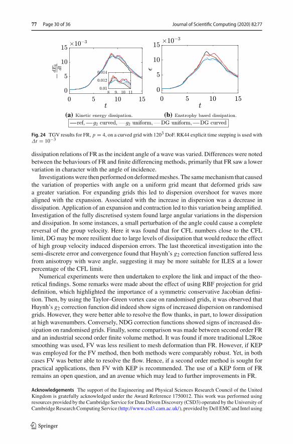
Applying this transformation to a 1203 DoF p = 4 mesh, results in qh = 0.7128 andΔxmax/Δxmin = 1.5—see Fig. 23. The result of applying a TGV to this grid are displayed inFig. 24. This shows that for both NDG and g2 the curved grid causes a larger variation in theenstrophy, mostly manifesting as over dissipation—and hence dispersion—at t ≈ 10. Thiserror is less for NDG but due to its presence in both correction functions, it may be concludedthat this grid deformation results in the increase in high frequency dispersion with FR.

7 Conclusions

Through this work, a theoretical extension of the FR von Neumann analysis to higher dimen-sions has been presented. This allowed us to understand the character of the dispersion and

123



Fig. 24 TGV results for FR, p = 4, on a curved grid with 1203 DoF. RK44 explicit time stepping is used withΔt = 10−3

dissipation relations of FR as the incident angle of a wave was varied. Differences were notedbetween the behaviours of FR and finite differencing methods, primarily that FR saw a lowervariation in character with the angle of incidence.

Investigationswere thenperformedondeformedmeshes.The samemechanism that causedthe variation of properties with angle on a uniform grid meant that deformed grids sawa greater variation. For expanding grids this led to dispersion overshoot for waves morealigned with the expansion. Associated with the increase in dispersion was a decrease indissipation. Application of an expansion and contraction led to this variation being amplified.Investigation of the fully discretised system found large angular variations in the dispersionand dissipation. In some instances, a small perturbation of the angle could cause a completereversal of the group velocity. Here it was found that for CFL numbers close to the CFLlimit, DGmay be more resilient due to large levels of dissipation that would reduce the effectof high group velocity induced dispersion errors. The last theoretical investigation into thesemi-discrete error and convergence found that Huynh’s g2 correction function suffered lessfrom anisotropy with wave angle, suggesting it may be more suitable for ILES at a lowerpercentage of the CFL limit.

Numerical experiments were then undertaken to explore the link and impact of the theo-retical findings. Some remarks were made about the effect of using RBF projection for griddefinition, which highlighted the importance of a symmetric conservative Jacobian defini-tion. Then, by using the Taylor–Green vortex case on randomised grids, it was observed thatHuynh’s g2 correction function did indeed show signs of increased dispersion on randomisedgrids. However, they were better able to resolve the flow thanks, in part, to lower dissipationat high wavenumbers. Conversely, NDG correction functions showed signs of increased dis-sipation on randomised grids. Finally, some comparison was made between second order FRand an industrial second order finite volume method. It was found if more traditional L2Roesmoothing was used, FV was less resilient to mesh deformation than FR. However, if KEPwas employed for the FV method, then both methods were comparably robust. Yet, in bothcases FV was better able to resolve the flow. Hence, if a second order method is sought forpractical applications, then FV with KEP is recommended. The use of a KEP form of FRremains an open question, and an avenue which may lead to further improvements in FR.

Acknowledgements The support of the Engineering and Physical Sciences Research Council of the UnitedKingdom is gratefully acknowledged under the Award Reference 1750012. This work was performed usingresources provided by the Cambridge Service for Data Driven Discovery (CSD3) operated by the University ofCambridgeResearchComputing Service (http://www.csd3.cam.ac.uk/), provided byDell EMCand Intel using

123

http://www.csd3.cam.ac.uk/


Tier-2 funding from the Engineering and Physical Sciences Research Council (Capital Grant EP/P020259/1),and DiRAC funding from the Science and Technology Facilities Council (www.dirac.ac.uk).

Open Access This article is licensed under a Creative Commons Attribution 4.0 International License, whichpermits use, sharing, adaptation, distribution and reproduction in any medium or format, as long as you giveappropriate credit to the original author(s) and the source, provide a link to the Creative Commons licence,and indicate if changes were made. The images or other third party material in this article are included in thearticle’s Creative Commons licence, unless indicated otherwise in a credit line to the material. If material isnot included in the article’s Creative Commons licence and your intended use is not permitted by statutoryregulation or exceeds the permitted use, you will need to obtain permission directly from the copyright holder.To view a copy of this licence, visit http://creativecommons.org/licenses/by/4.0/.

A Additional Dispersion and Dissipation FiguresWe include some additional figures that explore the effect of grid stretching in 2D, for thefully discretised Fourier analysis.

See Figs. 25 and 26.

123

www.dirac.ac.uk

http://creativecommons.org/licenses/by/4.0/


(a) Dispersion: γx = 1, γy = 1.1. (b) Dissipation: γx = 1, γy = 1.1.

(c) Dispersion: γx = 0.9, γy =1.1.

(d) Dissipation: γx = 0.9, γy =1.1.

Fig. 25 Dispersion and dissipation of upwindedFR, p = 3,withHuynh g2 corrections, explicit RK44 temporalintegration, and CFL = 0.8CFLmax. The radial distance is the normalised wavenumber (including the effectof angle), and the azimuthal distance is the angle of incidence to the element

123


(a) Dispersion: γx = 1, γy = 1.1. (b) Dissipation: γx = 1, γy = 1.1.

(c) Dispersion: γx = 0.9, γy =1.1.

(d) Dissipation: γx = 0.9, γy =1.1.

Fig. 26 Dispersion and dissipation of upwinded FR, p = 3, with NDG corrections, explicit RK44 temporalintegration, and CFL = 0.8CFLmax. The radial distance is the normalised wavenumber (including the effectof angle), and the azimuthal distance is the angle of incidence to the element

123


References

1. Abe, Y., Haga, T., Nonomura, T., Fujii, K.: On the freestream preservation of high-order conservativeflux-reconstruction schemes. J. Comput. Phys. 281, 28–54 (2015). https://doi.org/10.1016/j.jcp.2014.10.011

2. Abe,Y., Iizuka,N., Nonomura, T., Fujii, K.: Conservativemetric evaluation for high-order finite differenceschemes with the GCL identities on moving and deforming grids. J. Comput. Phys. 232(1), 14–21 (2013).https://doi.org/10.1016/j.jcp.2012.08.031

3. Adjerid, S., Devine, K.D., Flaherty, J.E., Krivodonova, L.: A posteriori error estimation for discontinuousGalerkin solutions of hyperbolic problems. Comput. Methods Appl. Mech. Eng. 191(11–12), 1097–1112(2002). https://doi.org/10.1016/S0045-7825(01)00318-8

4. Asthana, K., Watkins, J., Jameson, A.: On consistency and rate of convergence of flux reconstruction fortime-dependent problems. J. Comput. Phys. 334, 367–391 (2017). https://doi.org/10.1016/j.jcp.2017.01.008

5. Bassi, F., Rebay, S.: A high-order accurate discontinuous finite element method for the numerical solutionof the compressible Navier–Stokes equations. J. Comput. Phys. 131(2), 267–279 (1997). https://doi.org/10.1006/jcph.1996.5572

6. Bassi, F., Rebay, S.: An implicit high-order discountinuous Galerkin method for the steady state com-pressible Navier–Stokes equations. In: Computational FluidDynamics ’98, pp. 1226–1233.Wiley, Athens(1998)

7. Beckert, A.,Wendland, H.:Multivariate interpolation for fluid-structure-interaction problems using radialbasis functions. Aerosp. Sci. Technol. 5(2), 125–134 (2001)

8. Brachet, M.E., Merion, D.L., Orszag, S.A., Nickel, B.G., Morf, R.H., Frisch, U.: Small-scale structure ofthe Taylor–Green vortex. J. Fluid Mech. 130, 411–452 (1983)

9. Brandvik, T., Pullan, G.: An accelerated 3D Navier–Stokes solver for flows in turbomachines. J. Turbo-mach. 133(April 2011), 1–9 (2009). https://doi.org/10.1115/1.4001192

10. Brenner, S.C.,Ridgway-Scott, L.: TheMathematical Theory of FiniteElementMethods, 3rd edn. Springer,New York (2008)

11. Carr, J.C., Beatson, R.K., McCallum, B.C., Fright, W.R., McLennan, T.J., Mitchell, T.J.: Smooth surfacereconstruction from noisy range data. In: Proceedings of the 1st International Conference on ComputerGraphics and Interactive Techniques in Australasia and South East Asia. ACM (2003)

12. Castonguay, P.:High-order energy stableflux reconstruction schemes for fluidflowsimulations onunstruc-tured grids. Ph.D. thesis, Stanford University (2012)

13. Castonguay, P., Williams, D.M., Vincent, P.E., Jameson, A.: Energy stable flux reconstruction schemesfor advection–diffusion problems. Comput. Methods Appl. Mech. Eng. 267(1), 400–417 (2013). https://doi.org/10.1016/j.cma.2013.08.012

14. Chow, F.K., Moin, P.: A further study of numerical errors in large-eddy simulations. J. Comput. Phys.184(2), 366–380 (2003). https://doi.org/10.1016/S0021-9991(02)00020-7

15. Cockburn, B., Luskin, M., Shu, C.W., Suli, E.: Post-processing of Galerkin methods for hyperbolicproblems. In: Discontinuous Galerkin Methods (Newport, RI, 1999), pp. 291–300. Springer, Newport(1999)

16. Courant, R., Friedrichs, K., Lewy, H.: On the partial differnce equations of mathematical physics. IBMJ. 11(2), 215–234 (1967). https://doi.org/10.1147/rd.112.0215

17. Davis, S.: Simplified second-order Godunov-type methods. SIAM J. Sci. Stat. Comput. 9(3), 445–473(1988)

18. de Boer, A., van der Schoot, M.S., Bijl, H.: Mesh deformation based on radial basis function interpolation.Comput. Struct. 85(11–14), 784–795 (2007)

19. DeBonis, J.R.: Solutions of the Taylor–Green vortex problem using high-resolution explicit finite dif-ference methods. In: 51st AIAA Aerospace Sciences Meeting including the New Horizons Forum andAerospace Exposition (February 2013) (2013). https://doi.org/10.2514/6.2013-382

20. Duchon, J.: Splines minimizing rotation-invariant semi-norms in Sobolev spaces. In: Constructive Theoryof Functions of Several Variables, pp. 85–100. Springer (1977)

21. Ghosal, S.: An analysis of numerical errors in large-eddy simulations of turbulence. J. Comput. Phys.125(1), 187–206 (1996). https://doi.org/10.1006/jcph.1996.0088

22. Harten, A., Lax, P.D., van Leer, B.: On upstream differencing and Godunov-type schemes for hyperbolicconservation laws. SIAM Rev. 25(1), 35–61 (1983). https://doi.org/10.1137/1025002

23. Hesthaven, J.S.,Warburton, T.: NodalDiscontinuousGalerkinMethods:Algorithms,Analysis, andAppli-cations,Texts inAppliedMathematics, vol. 54, first edn. SpringerNewYork,NewYork,NY (2008). https://doi.org/10.1007/978-0-387-72067-8. http://link.springer.com/10.1007/978-0-387-72067-8

123

https://doi.org/10.1016/j.jcp.2014.10.011



https://doi.org/10.1016/S0045-7825(01)00318-8



https://doi.org/10.1006/jcph.1996.5572


https://doi.org/10.1115/1.4001192

https://doi.org/10.1016/j.cma.2013.08.012


https://doi.org/10.1016/S0021-9991(02)00020-7

https://doi.org/10.1147/rd.112.0215

https://doi.org/10.2514/6.2013-382


https://doi.org/10.1137/1025002

https://doi.org/10.1007/978-0-387-72067-8

https://doi.org/10.1007/978-0-387-72067-8

http://link.springer.com/10.1007/978-0-387-72067-8


24. Huynh, H.T.: A flux reconstruction approach to high-order schemes including discontinuous Galerkinmethods. In: 18th AIAA Computational Fluid Dynamics Conference, vol. 2007–4079, pp. 1–42 (2007).https://doi.org/10.2514/6.2007-4079

25. Isaacson, E., Keller, H.B.: Analysis of Numerical Methods, 2nd edn. Wiley, New York (1994). https://doi.org/10.2307/2003280

26. Jameson, A.: Formulation of kinetic energy preserving conservative schemes for gas dynamics anddirect numerical simulation of one-dimensional viscous compressible flow in a shock tube using entropyand kinetic energy preserving schemes. J. Sci. Comput. 34(2), 188–208 (2008). https://doi.org/10.1007/s10915-007-9172-6

27. Jameson, A., Vincent, P.E., Castonguay, P.: On the non-linear stability of flux reconstruction schemes. J.Sci. Comput. 50(2), 434–445 (2012). https://doi.org/10.1007/s10915-011-9490-6

28. Kopriva, D.A., Kolias, J.H.: A conservative staggered-grid Chebyshev multidomain method for com-pressible flows. J. Comput. Phys. 261(125), 244–261 (1996)

29. Kress, R.: Numerical Analysis. Graduate Texts in Mathematics, vol. 181, 1st edn. Springer, New York,NY (1998). https://doi.org/10.1007/978-1-4612-0599-9

30. Lax, P.D., Richtmyer, R.D.: Survey of the stability of linear finite difference equations. Commun. PureAppl. Math. IX(1), 267–293 (1956). https://doi.org/10.1002/cpa.3160090206

31. Lele, S.K.: Compact finite difference schemes with spectral-like resolution. J. Comput. Phys. 103(1),16–42 (1992). https://doi.org/10.1016/0021-9991(92)90324-R

32. Mengaldo, G., De Grazia, D., Vincent, P.E., Sherwin, S.J.: On the connections between discontinuousGalerkin and flux reconstruction schemes: extension to curvilinear meshes. J. Sci. Comput. 67(3), 1272–1292 (2016). https://doi.org/10.1007/s10915-015-0119-z

33. Oßwald, K., Siegmund, A., Birken, P., Hannemann, V., Meister, A.: L2 Roe: a low dissipation version ofRoe’s approximate Riemann solver for low Mach numbers. Int. J. Numer. Methods Fluids 81(2), 71–86(2016). https://doi.org/10.1002/fld.4175

34. Quarteroni, A.: Domain decomposition methods for systems of conservation laws: spectral collocationapproximations. SIAM J. Sci. Stat. Comput. 11(6), 1029–1052 (1990)

35. Reed, W.H., Hill, T.R.: Triangular mesh methods for the neutron transport equation. Technical ReportLA-UR-73-479 (1973)

36. Roe, P.L.: Approximate Riemann solvers, parameter vectors, and difference schemes. J. Comput. Phys.43, 357–372 (1981)

37. Rusanov, V.: The calculation of the interaction of non-stationary shock waves with barriers. Zh. Vychisl.Mat. Mat. Fiz. 1(2), 267–279 (1961). https://doi.org/10.18287/0134-2452-2015-39-4-453-458

38. Scillitoe, A.D., Tucker, P.G., Adami, P.: Numerical investigation of three-dimensional separation in anaxial flow compressor: the influence of freestream turbulence intensity and endwall boundary layer state.J. Turbomach. 139(2), 021011 (2016). https://doi.org/10.1115/1.4034797

39. Sheshadri, A.: An analysis of stability of the flux reconstruction formulation with applications to shockcapturing. Ph.D. thesis, Stanford University (2016)

40. Sheshadri, A., Jameson, A.: On the stability of the flux reconstruction schemes on quadrilateral elementsfor the linear advection equation. J. Sci. Comput. 67(2), 769–790 (2016). https://doi.org/10.1007/s10915-015-0102-8

41. Taylor, G.I., Green, A.E.: Mechanism of the production of small Eddies from large ones. Proc. R. Soc.A: Math. Phys. Eng. Sci. 158(895), 499–521 (1937). https://doi.org/10.1098/rspa.1937.0036

42. Thomas, P.D., Lombard, C.K.: Geometric conservation law and its application to flow computations onmoving grids. AIAA J. (2012). https://doi.org/10.2514/3.61273

43. Trojak, W.: Generalised Lebesgue stable flux reconstruction (2018). arXiv:1805.1248144. Trojak, W.: Generalised Sobolev stable flux reconstruction (2018). arXiv:1804.0471445. Trojak, W., Watson, R., Tucker, P.G.: High order flux reconstruction on stretched and warped meshes. In:

AIAA SciTech, 55th AIAA Aerospace Sciences Meeting, pp. 1–12. Grapevine Texas (2017)46. Trojak, W., Watson, R., Tucker, P.G.: Temporal stabilisation of flux reconstruction on linear problems.

In: 2018 Fluid Dynamics Conference, AIAA AVIATION Forum. American Institute of Aeronautics andAstronautics, Atlanta (2018). https://doi.org/10.2514/6.2018-4263

47. Trojak, W., Watson, R., Tucker, P.G.: High-order flux reconstruction on stretched and warped meshes.AIAA J. 57(1), 341–351 (2019). https://doi.org/10.2514/1.J056341

48. Trojak, W., Witherden, F.D.: A new family of weighted one-parameter flux reconstruction schemes, pp.1–37 (2018). arXiv:1809.07846

49. van Leer, B.: Flux-vector splitting for the Euler equation. Technical Report February (1982). https://doi.org/10.1007/3-540-11948-5

123

https://doi.org/10.2514/6.2007-4079

https://doi.org/10.2307/2003280

https://doi.org/10.2307/2003280

https://doi.org/10.1007/s10915-007-9172-6

https://doi.org/10.1007/s10915-007-9172-6

https://doi.org/10.1007/s10915-011-9490-6

https://doi.org/10.1007/978-1-4612-0599-9

https://doi.org/10.1002/cpa.3160090206

https://doi.org/10.1016/0021-9991(92)90324-R

https://doi.org/10.1007/s10915-015-0119-z

https://doi.org/10.1002/fld.4175

https://doi.org/10.18287/0134-2452-2015-39-4-453-458

https://doi.org/10.1115/1.4034797

https://doi.org/10.1007/s10915-015-0102-8

https://doi.org/10.1007/s10915-015-0102-8

https://doi.org/10.1098/rspa.1937.0036

https://doi.org/10.2514/3.61273

http://arxiv.org/abs/1805.12481


https://doi.org/10.2514/6.2018-4263

https://doi.org/10.2514/1.J056341


https://doi.org/10.1007/3-540-11948-5

https://doi.org/10.1007/3-540-11948-5


50. van Rees, W.M., Leonard, A., Pullin, D., Koumoutsakos, P.: A comparison of vortex and pseudo-spectralmethods for the simulation of periodic vortical flows at high Reynolds numbers. J. Comput. Phys. 230(8),2794–2805 (2011). https://doi.org/10.1016/j.jcp.2010.11.031

51. Vermeire, B.C., Vincent, P.E.: On the behaviour of fully-discrete flux reconstruction schemes. J. Comput.Phys. 315(1), 1053–1079 (2017). https://doi.org/10.1016/j.jcp.2016.09.034

52. Vincent, P.E., Castonguay, P., Jameson, A.: A new class of high-order energy stable flux reconstructionschemes. J. Sci. Comput. 47(1), 50–72 (2010). https://doi.org/10.1007/s10915-010-9420-z

53. Vincent, P.E., Castonguay, P., Jameson, A.: Insights from von Neumann analysis of high-order fluxreconstruction schemes. J. Comput. Phys. 230(22), 8134–8154 (2011). https://doi.org/10.1016/j.jcp.2011.07.013

54. Vincent, P.E., Farrington, A.M., Witherden, F.D., Jameson, A.: An extended range of stable-symmetric-conservative flux reconstruction correction functions. Comput. Methods Appl. Mech. Eng. 296, 248–272(2015). https://doi.org/10.1016/j.cma.2015.07.023

55. Vincent, P.E., Witherden, F.D., Vermeire, B.C., Park, J.S., Iyer, A.: Towards Green Aviation with Pythonat Petascale. In: International Conference for High Performance Computing, Networking, Storage andAnalysis, SC, November, pp. 1–11. IEEE, Denver (2017). https://doi.org/10.1109/SC.2016.1

56. Wang, Z.J.: Spectral (finite) volume method for conservation laws on unstructured grids. Basic formu-lation: basic formulation. J. Comput. Phys. 178(1), 210–251 (2002). https://doi.org/10.1006/jcph.2002.7041

57. Watson, R.A., Tucker, P.G., Wang, Z.N., Yuan, X.: Towards robust unstructured turbomachinery largeEddy simulation. Comput. Fluids 118, 245–254 (2015). https://doi.org/10.1016/j.compfluid.2015.06.017

58. Williams, D.M., Jameson, A.: Erratum to: Energy stable flux reconstruction schemes for advection–diffusion problems on tetrahedra. J. Sci. Comput. 59, 760 (2014). https://doi.org/10.1007/s10915-013-9789-6

59. Yu, M., Wang, Z.J., Liu, Y.: On the accuracy and efficiency of discontinuous Galerkin, spectral differenceand correction procedure via reconstruction methods. J. Comput. Phys. 259, 70–95 (2014). https://doi.org/10.1016/j.jcp.2013.11.023

60. Zhang, H., Reggio, M., Trépanier, J.Y., Camarero, R.: Discrete form of the GCL for moving meshes andits implementation in CFD schemes. Comput. Fluids 22(1), 9–23 (1993). https://doi.org/10.1016/0045-7930(93)90003-R

Publisher’s Note Springer Nature remains neutral with regard to jurisdictional claims in published maps andinstitutional affiliations.

123



https://doi.org/10.1007/s10915-010-9420-z




https://doi.org/10.1109/SC.2016.1



https://doi.org/10.1016/j.compfluid.2015.06.017

https://doi.org/10.1007/s10915-013-9789-6

https://doi.org/10.1007/s10915-013-9789-6



https://doi.org/10.1016/0045-7930(93)90003-R

https://doi.org/10.1016/0045-7930(93)90003-R

Effect of Mesh Quality on Flux Reconstruction in …...FR is found to be more resilient to mesh...

Documents

Transcript of Effect of Mesh Quality on Flux Reconstruction in …...FR is found to be more resilient to mesh...