26th Symposium on Naval Hydrodynamics Rome, Italy, 17-22 September 2006

Effect of Gas Diffusion on Bubble Entrainment and Dynamics around a Propeller

C.-T. Hsiao, A. Jain, and G. L. Chahine (DYNAFLOW, INC., USA)

ABSTRACT

A multi-bubble dynamics code accounting for gas diffusion across the bubble wall was developed and used to study bubble nuclei population dynamics in the flow field of a propeller. The propeller flow field was obtained using a Reynolds-Averaged Navier-Stokes (RANS) solver and bubble nuclei populations was propagated in this field. The code developed enables one to investigate the possibility of generating behind a propeller long lasting visible bubble starting from an ocean nuclei size distribution. Large visible bubbles are seen to cluster in the tip vortices and in the wakes of the blades. Parametric investigation of the initial nuclei size distribution, the dissolved gas concentration, and the cavitation number were conducted to identify their effects on bubble entrainment, and void fraction and bubble distribution modification downstream from the propeller. Artificial turbulence-like fluctuations were also superimposed unto the RANS flow field to study whether RANS averaging significantly affects the results.

1. Introduction

The generation and entrainment of bubbles from a surface ship is not completely understood despite the fact that it affects the safety of the ship. These bubbles are transported by the flow field to the stern area, captured in the ship wake, trapped in the large vortical structures, and then act as tracers of the ship wake. In littoral warfare, such bubbly wakes provide an excellent opportunity to homing devices enabling them to easily find their target because of the large acoustic cross sections and high acoustic response of bubbles to acoustic waves.

It is commonly thought that bubble entrainment has two main sources. One source is from bubbles generated by air entrainment due to free surface and hull interactions such as breaking and spilling waves at the bow and stern and boundary layer entrainment along the hull. The other potential source

is bubble production by the propellers. While there have been some research efforts to understand and observe bubble generation and entrainment in breaking waves (e.g. Waniewski and Brennen, 2000, Carrica et al., 1999, Paterson et al., 1996), much less has been done to investigate the other means of bubble generation/entrainment.

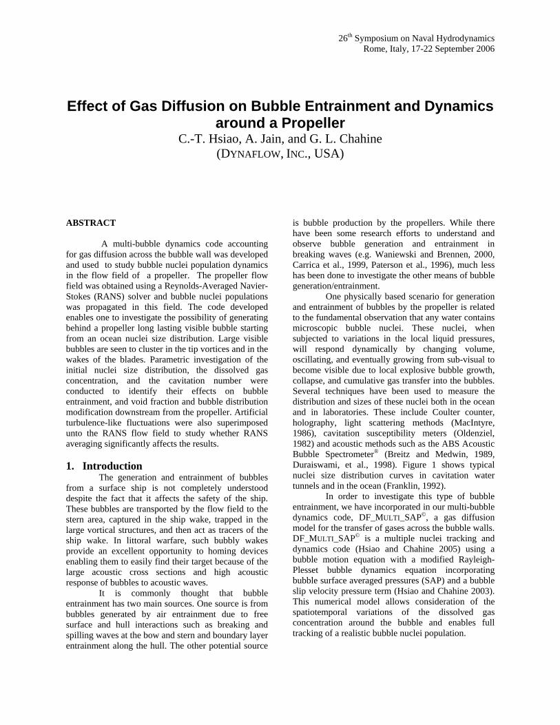
One physically based scenario for generation and entrainment of bubbles by the propeller is related to the fundamental observation that any water contains microscopic bubble nuclei. These nuclei, when subjected to variations in the local liquid pressures, will respond dynamically by changing volume, oscillating, and eventually growing from sub-visual to become visible due to local explosive bubble growth, collapse, and cumulative gas transfer into the bubbles. Several techniques have been used to measure the distribution and sizes of these nuclei both in the ocean and in laboratories. These include Coulter counter, holography, light scattering methods (MacIntyre, 1986), cavitation susceptibility meters (Oldenziel, 1982) and acoustic methods such as the ABS Acoustic Bubble Spectrometer® (Breitz and Medwin, 1989, Duraiswami, et al., 1998). Figure 1 shows typical nuclei size distribution curves in cavitation water tunnels and in the ocean (Franklin, 1992).

In order to investigate this type of bubble entrainment, we have incorporated in our multi-bubble dynamics code, DF_MULTI_SAP©, a gas diffusion model for the transfer of gases across the bubble walls. DF_MULTI_SAP© is a multiple nuclei tracking and dynamics code (Hsiao and Chahine 2005) using a bubble motion equation with a modified Rayleigh-Plesset bubble dynamics equation incorporating bubble surface averaged pressures (SAP) and a bubble slip velocity pressure term (Hsiao and Chahine 2003). This numerical model allows consideration of the spatiotemporal variations of the dissolved gas concentration around the bubble and enables full tracking of a realistic bubble nuclei population.

To investigate bubble production by the propeller, we have utilized this model to propagate a nuclei distribution in the flow field of a marine propeller (NSWCCD Propeller 5168). The flow field was simulated by Hsiao and Pauley (1999) using a Reynolds-Averaged Navier-Stokes solver and validated using experimental measurements obtained by Chesnakas and Jessup (1998).

Figure 1. Nuclei Size distribution as measured in the ocean and in the laboratory (from Franklin, 1992).

2. Numerical Approach 2.1 Bubble Dynamics Model

The dynamics of a spherical bubble has been extensively studied following the original works of Rayleigh (1917) and Plesset (1964) which included for an incompressible liquid, the effects of inertia, bubble content compressibility, and ambient pressure variations. Since then, a very large number of studies have been conducted to include a host of other physical phenomena. In the present study we have considered the following form of the equation for the bubble radius, R(t), which accounts for liquid and gas compressibility, liquid viscosity, surface tension, and non-uniform pressure fields, and is based on Gilmore’s approach (Gilmore, 1952).

( )2

3 1(1 ) (1 ) (1 )2 3

2 4 ,4

enc bv g encounter

R R R R dRR Rc c c c dt

Rp p pR R

ρ

γ µ

− + − = + +

−⎡ ⎤+ − − − +⎢ ⎥

⎣ ⎦

u u(1)

where c is the sound speed, ρ is the liquid density, µ is the liquid viscosity, pv is the vapor pressure, pg is the gas pressure, γ is the surface tension, pencounter and uenc are the liquid pressure and velocity respectively, and

bu is the bubble travel velocity. In Equation (1), which we dub the Surface-Averaged Pressure (SAP) bubble dynamics equation (Hsiao and Chahine 2003), we have accounted for a slip velocity between the bubble and the host liquid, and for a non-uniform

pressure field along the bubble surface. encounterP and uenc are defined as the average of the liquid pressures and velocities over the bubble surface. The use of

encounterP results in a major improvement over the classical spherical bubble model which uses the pressure at the bubble center in its absence. The gas pressure, pg, is obtained, as described in the next section, from the solution of the gas diffusion problem and the assumption that the gas is an ideal gas.

The bubble trajectory is obtained using the following motion equation (Johnson and Hsieh 1966):

( )

( )

b 3 34

3 ,

Denc b enc b

enc b

d CPdt R

RR

ρ= − ∇ + − −

+ −

u u u u u

u u (2)

where CD is the drag coefficient given by an empirical equation such as that of Haberman and Morton (1953):

0.63 4 1.3824 (1 0.197 2.6 10 ),

2.

D eb ebeb

enc beb

C R RR

RR

ρµ

−= + + ×

−=

u u (3)

The last term on the right hand side of Equation (3) is the force due to the bubble volume variations, which is obtained by solving Equation (1).

2.2 Gas Diffusion Model

Water can contain gas not only in the form of nuclei with a particular distribution, but also as a dissolved gas with a concentration C. In the presence of a local concentration gradient, dissolved gas will diffuse from the high concentration to the low concentration region. The transport equation for the time and space dependent dissolved gas concentration, C, in the liquid is given by:

2 ,gC C D Ct

∂+ ⋅∇ = ∇

∂u (4)

where Dg is the molar diffusivity of the gaseous component in the liquid (in practice the turbulent diffusivity is also used in high turbulence areas). Concerning bubble dynamics, the following initial and far field boundary conditions apply:

0 for ,for ,

C C t tC C r

∞

∞

= =

→ →∞ (5)

Where r is the distance from the bubble center and C∞ is the dissolved gas concentration far away from the bubble surface.

The conditions at the bubble interface are very important and actually drive the gas diffusion. The first condition states that the gas concentration in

the liquid at the interface is the saturation gas concentration:

at .sC C r R= = (6) where Cs is the dissolved gas concentration at the bubble surface on the liquid side. The saturation concentration is connected to the partial gas pressure, pg, through Henry’s law:

,g sp HC= (7) where H is the Henry constant. In addition, we write an equation of gas transfer at the bubble/liquid interface:

.g gSCD dS nn

∂=

∂∫ (8)

This equation directly connects the diffusion of gas at the interface with the interfacial area and the transfer rate of gas moles, gn , between the liquid and the bubble.

Since numerical solution of Equation (5) requires gridding of the full space, Plesset and Zwick (1953) introduced a very useful approximation in the case where the changes in gas concentration are restricted to a boundary layer around the bubble. An analytical solution then exists and relates the gas concentration at the bubble wall to the concentration at “infinity”. This expression requires integration over the whole history of the bubble dynamics in order to enable computation of the amount of gas inside the bubble, and has the following form:

( )0 1/ 24

1 .4

gts

tg

nC C d

D R y dyτ

τπ π∞= −

⎡ ⎤⎢ ⎥⎣ ⎦

∫∫

(9)

One should note that to solve the bubble volume Equation (1) we need the gas pressure, pg, and to get pg we need the history of the variations of the bubble radius and the rate of transfer of gas moles,

gn , across the bubble interface. The problem is closed by considering the

thermodynamics of the contents of the bubble. The two components of the bubble content: vapor and gas, are both assumed to be ideal gases which follow an ideal gas law:

; ,

( / ).g b g u b v b v u b

v g v g

p V n R T p V n R T

n n p p

= =

= (10)

One consequence of this assumption is that the amount of gas, ng, and vapor, nv, in the bubble are directly proportional to the ratio of their respective partial pressures. Since these quantities change in time because of both mass exchange and compression/ expansion, we consider their dynamics through the thermodynamics inside the bubble and energy balance on the bubble control volume.

,

,i ii v g

dU dW n h dt=

= − + ∑ (11)

wherev,i

,

p,i,

c ( ) is change in internal energy,

= ( ) is work done by control volume,

= c is specific enthalpy.

i ii v g

v g b

i i li v g

dU d n T

dW p p dV

h n T

=

=

=

+

∑

∑

Chahine et al. (1987a, b) reduced the equations of determining pg to the following two differential equations:

( )2

/,

/

with , , , , , , ,

g gg

g

g gg

E p Dp Fp

A B p

A B D E F f R R n n

− −=

+

=

(12)

( )

2

0 1/ 24( ) .

124

ggt h

gt h

g

PC nR Hn t d

h R y dyD τ

τ

π π

∞ −

−

⎡ ⎤⎢ ⎥−⎢ ⎥= −⎢ ⎥⎡ ⎤⎢ ⎥⎢ ⎥⎣ ⎦⎢ ⎥⎣ ⎦

∫∫

(13)

To determine each bubble motion and volume variation, the set of four differential Equations (1), (2), (12), and (13) are solved using a Runge-Kutta fourth-order scheme to integrate through time. 3. Results and Discussion

In this study, nuclei with a prescribed void fraction were released upstream from a rotating propeller and then tracked using DF_MULTI_SAP© through the computational domain. The propeller model is the David Taylor Propeller 5168 which is a five-blade propeller with a 15.856 inch (0.4 m) diameter. The flow field around this propeller was simulated for three different advance coefficients (Hsiao and Pauley, 1999) using a Reynolds-Averaged Navier-Stokes solver and were validated against experimental measurements conducted by Chesnakas and Jessup (1998). The flow field used in the study has an advance coefficient /J U nD∞= = 1.1 where U∞ = 10.7 m/s, n = 1450 rpm, and D is the propeller diameter.

3.1 Gas Diffusion Effects

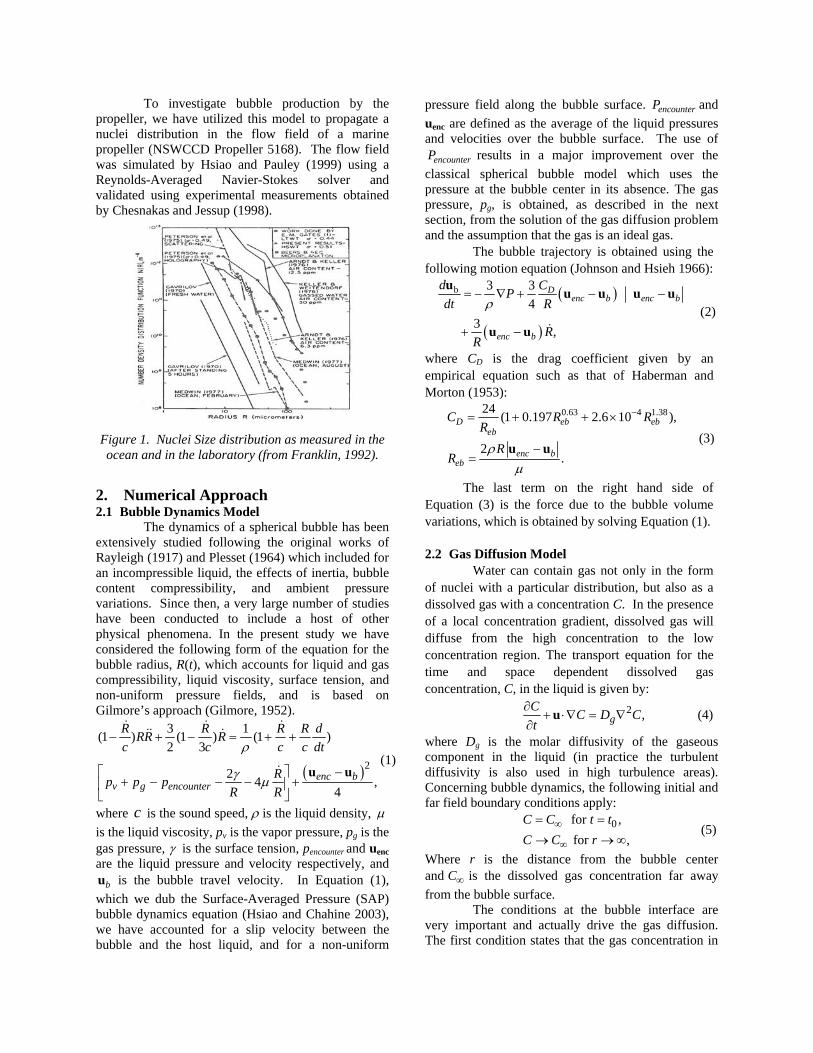
To study the gas diffusion effects on the bubble dynamics and the size distribution downstream from the propeller, we conducted first two sets of computations with “synthetic” bubble distributions: one set with and one set without including gas diffusion effects. Nuclei with a uniform radius of 50 µm were released from a preset grid located upstream from the propeller at x = -0.08 m as illustrated in Figure 2. The total number of bubble released was 4500. The tracking of each bubble started

from x = -0.08 m and ended at x = 0.3 m. The water was assumed to be supersaturated (i.e. the dissolved gas concentration was 100%, i.e. 0.66 mol/m3 of dissolved air), when gas diffusion was taken into account.

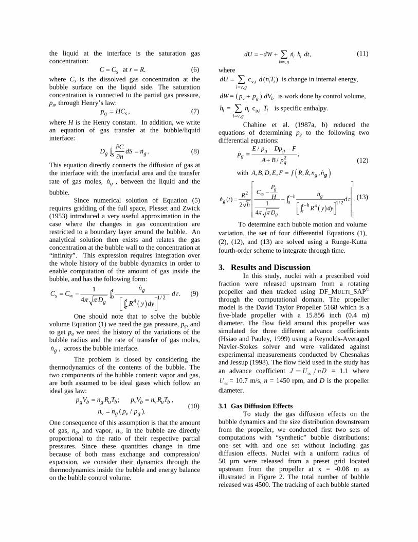
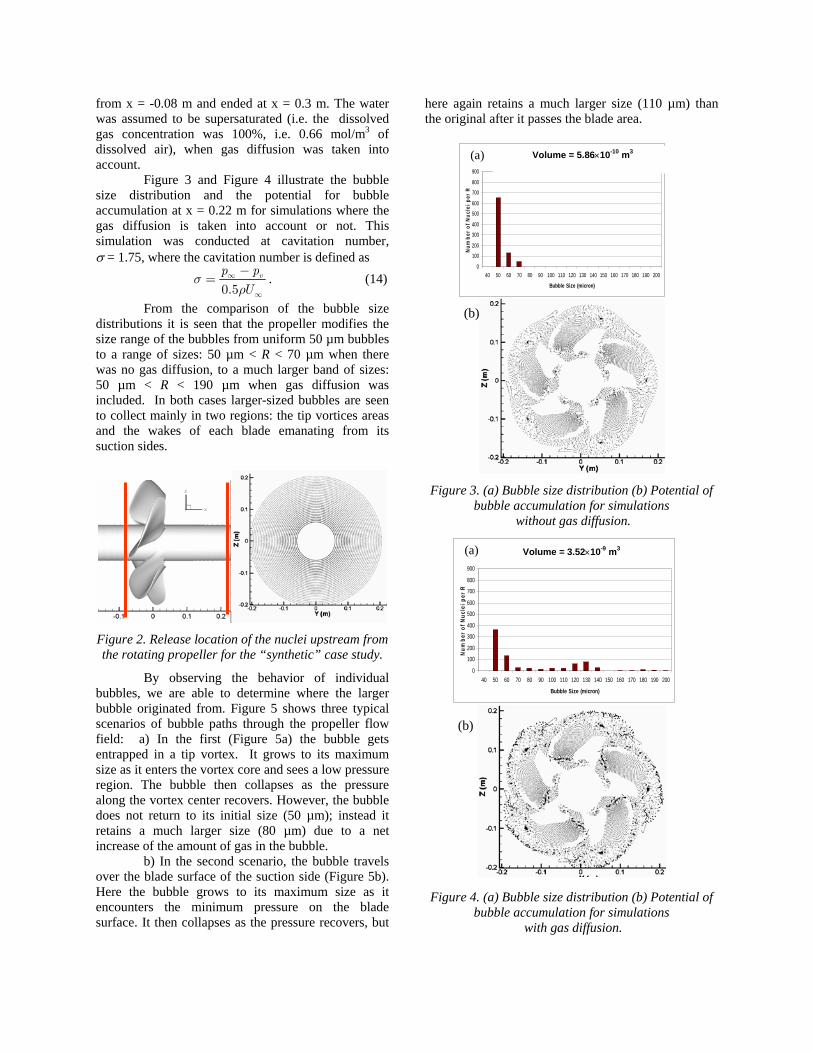
Figure 3 and Figure 4 illustrate the bubble size distribution and the potential for bubble accumulation at x = 0.22 m for simulations where the gas diffusion is taken into account or not. This simulation was conducted at cavitation number, σ = 1.75, where the cavitation number is defined as

0.5

vp pU

σρ

∞

∞

−= . (14)

From the comparison of the bubble size distributions it is seen that the propeller modifies the size range of the bubbles from uniform 50 µm bubbles to a range of sizes: 50 µm < R < 70 µm when there was no gas diffusion, to a much larger band of sizes: 50 µm < R < 190 µm when gas diffusion was included. In both cases larger-sized bubbles are seen to collect mainly in two regions: the tip vortices areas and the wakes of each blade emanating from its suction sides.

Figure 2. Release location of the nuclei upstream from the rotating propeller for the “synthetic” case study.

By observing the behavior of individual bubbles, we are able to determine where the larger bubble originated from. Figure 5 shows three typical scenarios of bubble paths through the propeller flow field: a) In the first (Figure 5a) the bubble gets entrapped in a tip vortex. It grows to its maximum size as it enters the vortex core and sees a low pressure region. The bubble then collapses as the pressure along the vortex center recovers. However, the bubble does not return to its initial size (50 µm); instead it retains a much larger size (80 µm) due to a net increase of the amount of gas in the bubble.

b) In the second scenario, the bubble travels over the blade surface of the suction side (Figure 5b). Here the bubble grows to its maximum size as it encounters the minimum pressure on the blade surface. It then collapses as the pressure recovers, but

here again retains a much larger size (110 µm) than the original after it passes the blade area.

Figure 3. (a) Bubble size distribution (b) Potential of

bubble accumulation for simulations without gas diffusion.

Figure 4. (a) Bubble size distribution (b) Potential of

bubble accumulation for simulations with gas diffusion.

X = 0.22 m

0

100

200

300

400

500

600

700

800

900

40 50 60 70 80 90 100 110 120 130 140 150 160 170 180 190 200

Bubble Size (micron)

Num

ber

of N

ucle

i per

R

Volume = 5.86×10-10 m3 (a)

X = 0.22 m

0

100

200

300

400

500

600

700

800

900

40 50 60 70 80 90 100 110 120 130 140 150 160 170 180 190 200

Bubble Size (micron)

Num

ber

of N

ucle

i per

R

Volume = 3.52×10-9 m3 (a)

(b)

(b)

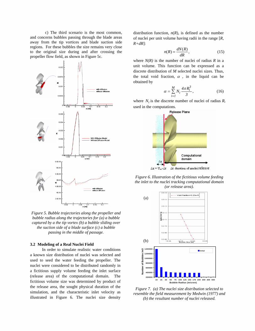
c) The third scenario is the most common, and concerns bubbles passing through the blade areas away from the tip vortices and blade suction side regions. For these bubbles the size remains very close to the original size during and after crossing the propeller flow field, as shown in Figure 5c.

Figure 5. Bubble trajectories along the propeller and bubble radius along the trajectories for (a) a bubble captured by a the tip vortex (b) a bubble sliding over

the suction side of a blade surface (c) a bubble passing in the middle of passage.

3.2 Modeling of a Real Nuclei Field

In order to simulate realistic water conditions a known size distribution of nuclei was selected and used to seed the water feeding the propeller. The nuclei were considered to be distributed randomly in a fictitious supply volume feeding the inlet surface (release area) of the computational domain. The fictitious volume size was determined by product of the release area, the sought physical duration of the simulation, and the characteristic inlet velocity as illustrated in Figure 6. The nuclei size density

distribution function, n(R), is defined as the number of nuclei per unit volume having radii in the range [R, R+dR]:

( )( ) ,dN Rn RdR

= (15)

where N(R) is the number of nuclei of radius R in a unit volume. This function can be expressed as a discrete distribution of M selected nuclei sizes. Thus, the total void fraction, α , in the liquid can be obtained by

3Mi

ii 1

4 RN

3π

α=

= ∑ , (16)

where iN is the discrete number of nuclei of radius Ri

used in the computations.

Figure 6. Illustration of the fictitious volume feeding the inlet to the nuclei tracking computational domain

(or release area).

Figure 7. (a) The nuclei size distribution selected to

resemble the field measurement by Medwin (1977) and (b) the resultant number of nuclei released.

200000

400000

600000

800000

1000000

1200000

1400000

10 15 30 50 75 100 125 150 175 200 300 400 500Bubble Radius (micron)

Num

ber o

f Bub

bles

/m3

Initial

(a)

(b)

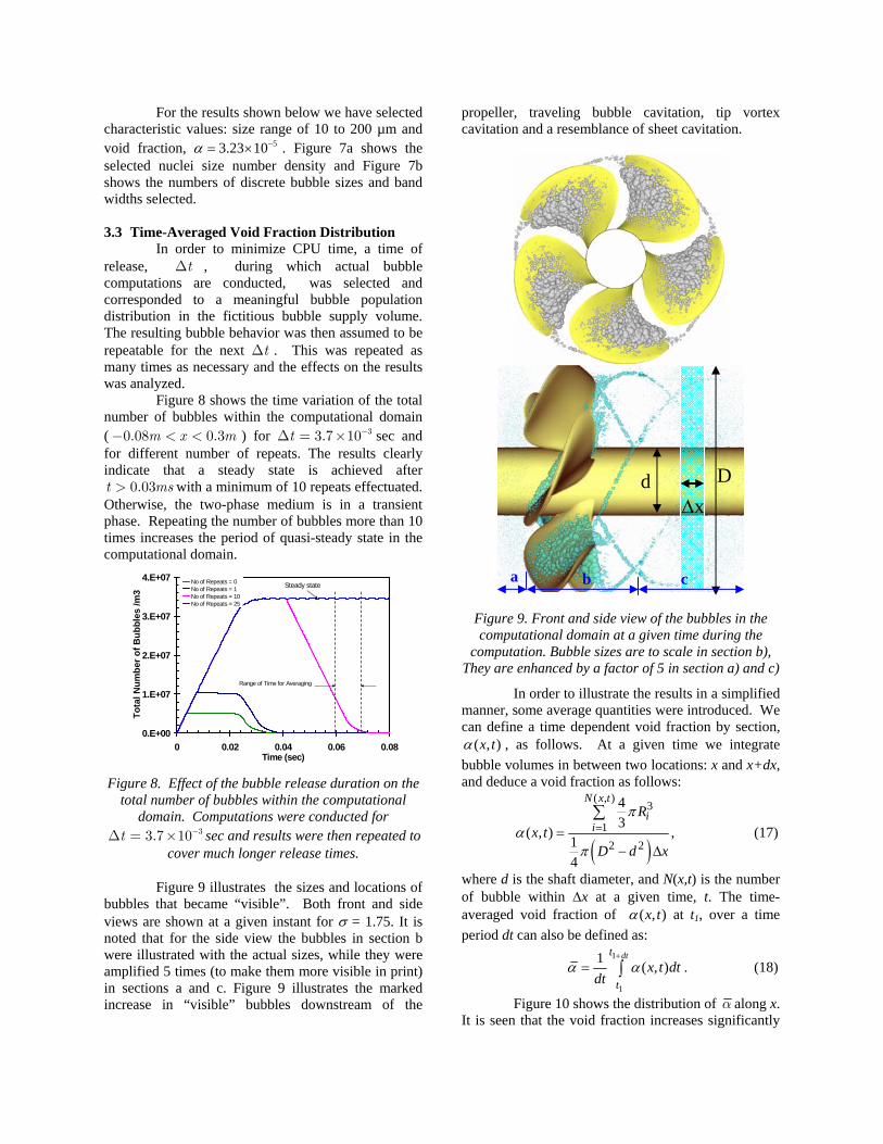
For the results shown below we have selected characteristic values: size range of 10 to 200 µm and void fraction, 53.23 10α −= × . Figure 7a shows the selected nuclei size number density and Figure 7b shows the numbers of discrete bubble sizes and band widths selected. 3.3 Time-Averaged Void Fraction Distribution

In order to minimize CPU time, a time of release, t∆ , during which actual bubble computations are conducted, was selected and corresponded to a meaningful bubble population distribution in the fictitious bubble supply volume. The resulting bubble behavior was then assumed to be repeatable for the next t∆ . This was repeated as many times as necessary and the effects on the results was analyzed.

Figure 8 shows the time variation of the total number of bubbles within the computational domain ( 0.08 0.3m x m− < < ) for 33.7 10t −∆ = × sec and for different number of repeats. The results clearly indicate that a steady state is achieved after 0.03t ms> with a minimum of 10 repeats effectuated.

Otherwise, the two-phase medium is in a transient phase. Repeating the number of bubbles more than 10 times increases the period of quasi-steady state in the computational domain.

Figure 8. Effect of the bubble release duration on the

total number of bubbles within the computational domain. Computations were conducted for

33.7 10t −∆ = × sec and results were then repeated to cover much longer release times.

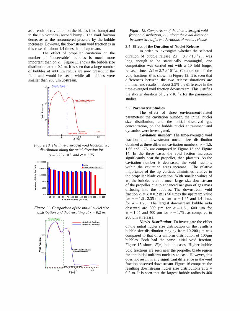
Figure 9 illustrates the sizes and locations of bubbles that became “visible”. Both front and side views are shown at a given instant for σ = 1.75. It is noted that for the side view the bubbles in section b were illustrated with the actual sizes, while they were amplified 5 times (to make them more visible in print) in sections a and c. Figure 9 illustrates the marked increase in “visible” bubbles downstream of the

propeller, traveling bubble cavitation, tip vortex cavitation and a resemblance of sheet cavitation.

Figure 9. Front and side view of the bubbles in the computational domain at a given time during the

computation. Bubble sizes are to scale in section b), They are enhanced by a factor of 5 in section a) and c)

In order to illustrate the results in a simplified manner, some average quantities were introduced. We can define a time dependent void fraction by section,

( , )x tα , as follows. At a given time we integrate bubble volumes in between two locations: x and x+dx, and deduce a void fraction as follows:

( )

( , )3

12 2

43

( , ) , 14

N x ti

iR

x tD d x

πα

π

==− ∆

∑ (17)

where d is the shaft diameter, and N(x,t) is the number of bubble within ∆x at a given time, t. The time-averaged void fraction of ( , )x tα at t1, over a time period dt can also be defined as:

1

1

1 ( , )dtt

tx t dt

dtα α

+

= ∫ . (18)

Figure 10 shows the distribution of α along x. It is seen that the void fraction increases significantly

0.E+00

1.E+07

2.E+07

3.E+07

4.E+07

0 0.02 0.04 0.06 0.08Time (sec)

Tota

l Num

ber o

f Bub

bles

/m3

No of Repeats = 0No of Repeats = 1No of Repeats = 10No of Repeats = 25

Range of Time for Averaging

Steady state

∆x Dd

a b c

as a result of cavitation on the blades (first hump) and in the tip vortices (second hump). The void fraction decreases as the encountered pressure by the bubble increases. However, the downstream void fraction is in this case still about 1.4 times that of upstream.

The effect of propeller cavitation on the number of “observable” bubbles is much more important than on α . Figure 11 shows the bubble size distribution at x = 0.2 m. It is seen that a large number of bubbles of 400 µm radius are now present in the field and would be seen, while all bubbles were smaller than 200 µm upstream.

Figure 10. The time-averaged void fraction, α ,

distribution along the axial direction for 53.23 10α −= × and σ = 1.75.

Figure 11. Comparison of the initial nuclei size

distribution and that resulting at x = 0.2 m.

Figure 12. Comparison of the time-averaged void fraction distribution, α , along the axial direction between two different durations of nuclei release.

3.4 Effect of the Duration of Nuclei Release In order to investigate whether the selected

duration of bubble release, 33.7 10 .t s−∆ = × , was long enough to be statistically meaningful, one computation was carried out with a 10 fold longer release time, 23.7 10 .t s−∆ = × Comparison of the void fractions α is shown in Figure 12. It is seen that differences between the two release durations are minimal and results in about 2.5% the difference in the time-averaged void fraction downstream. This justifies the shorter duration of 33.7 10 .s−× for the parametric studies. 3.5 Parametric Studies

The effect of three environment-related parameters: the cavitation number, the initial nuclei size distribution, and the initial dissolved gas concentration, on the bubble nuclei entrainment and dynamics were investigated.

Cavitation number: The time-averaged void fraction and downstream nuclei size distribution obtained at three different cavitation numbers, σ = 1.5, 1.65 and 1.75, are compared in Figure 13 and Figure 14. In the three cases the void faction increases significantly near the propeller, then plateaus. As the cavitation number is decreased, the void fractions within the cavitation areas increase. The relative importance of the tip vortices diminishes relative to the propeller blade cavitation. With smaller values of σ , the bubbles retain a much larger size downstream of the propeller due to enhanced net gain of gas mass diffusing into the bubbles. The downstream void fraction α at x = 0.2 m is 50 times the upstream value for 1.5σ = , 2.35 times for 1.65σ = and 1.4 times for 1.75σ = . The largest downstream bubble radii observed are 800 µm for 1.5σ = , 600 µm for

1.65σ = and 400 µm for 1.75σ = , as compared to 200 µm at release.

Nuclei Distribution: To investigate the effect of the initial nuclei size distribution on the results a bubble size distribution ranging from 10-200 µm was compared to that of a uniform distribution of 100µm bubbles. Both had the same initial void fraction. Figure 15 shows ( )xα in both cases. Higher bubble void fractions are seen near the propeller blade region for the initial uniform nuclei size case. However, this does not result in any significant difference in the void fraction observed downstream. Figure 16 compares the resulting downstream nuclei size distributions at x = 0.2 m. It is seen that the largest bubble radius is 400

100

1000

10000

100000

1000000

10000000

10 15 30 50 75 100 125 150 175 200 300 400 500Bubble Radius (micron)

Num

ber o

f Bub

bles

/m3 In itial

Downstream (X = 0.2)

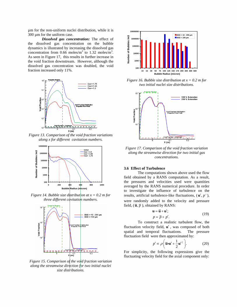
µm for the non-uniform nuclei distribution, while it is 300 µm for the uniform case.

Dissolved gas concentration: The effect of the dissolved gas concentration on the bubble dynamics is illustrated by increasing the dissolved gas concentration from 0.66 moles/m3 to 1.32 moles/m3. As seen in Figure 17, this results in further increase in the void fraction downstream. However, although the dissolved gas concentration was doubled, the void fraction increased only 11%.

Figure 13. Comparison of the void fraction variations

along x for different cavitation numbers.

Figure 14. Bubble size distribution at x = 0.2 m for

three different cavitation numbers.

Figure 15. Comparison of the void fraction variation along the streamwise direction for two initial nuclei

size distributions.

Figure 16. Bubble size distribution at x = 0.2 m for

two initial nuclei size distributions.

Figure 17. Comparison of the void fraction variation

along the streamwise direction for two initial gas concentrations.

3.6 Effect of Turbulence

The computations shown above used the flow field obtained by a RANS computation. As a result, the pressures and velocities used were quantities averaged by the RANS numerical procedure. In order to investigate the influence of turbulence on the results, artificial turbulence-like fluctuations, ( , 'p′u ), were randomly added to the velocity and pressure field, ( , pu ), obtained by RANS:

;.p p p′= +′= +

u u u (19)

To construct a realistic turbulent flow, the fluctuation velocity field, ′u , was composed of both spatial and temporal fluctuations. The pressure fluctuation field were then approximated by:

212

p ρ ⎛ ⎞′ ′ ′∝ +⎜ ⎟⎝ ⎠

u u ui . (20)

For simplicity, the following expressions give the fluctuating velocity field for the axial component only:

100

1000

10000

100000

1000000

10000000

10 15 30 50 75 100 125 150 175 200 300 400 500Bubble Radius (micron)

Num

ber o

f Bub

bles

/m3 BSD = 10 - 200 µm

BSD = 100 µm

100

1000

10000

100000

1000000

10000000

0 200 400 600 800 1000

Bubble Radius (micron)

Num

ber o

f Bub

bles

/m3 Initial

Cav = 1.5Cav = 1.65Cav= 1.75

( )( )

1

1

2

1

( , ) ( ) ( ) ( ) ( ) ,

1 2( ) cos 2 ( ) ,

1 2( ) cos 2 ( ) ,

1( ) cos 2 2 .

u

N y

yiiy yi

Nz

ziiz zi

Nt

i iit

i peaka

u t A f y f z f t U

yf yA

zf zA

f t e tA

ω ω

π πφ λλ

π πφ λλ

πω πφ ω

∞

=

=

⎛ ⎞⎜ ⎟−⎜ ⎟⎝ ⎠

=

−

′ = Ω

⎛ ⎞= +⎜ ⎟⎜ ⎟

⎝ ⎠⎛ ⎞

= +⎜ ⎟⎝ ⎠

= +

∑

∑

∑

x

(21)

To make the artificial fluctuations physics-based, their intensity Au(Ω) was related to the RANS determined vorticity distribution, Ω, and made maximum at Ωmax:

max

( ) .uA AΩ

Ω =Ω

(22)

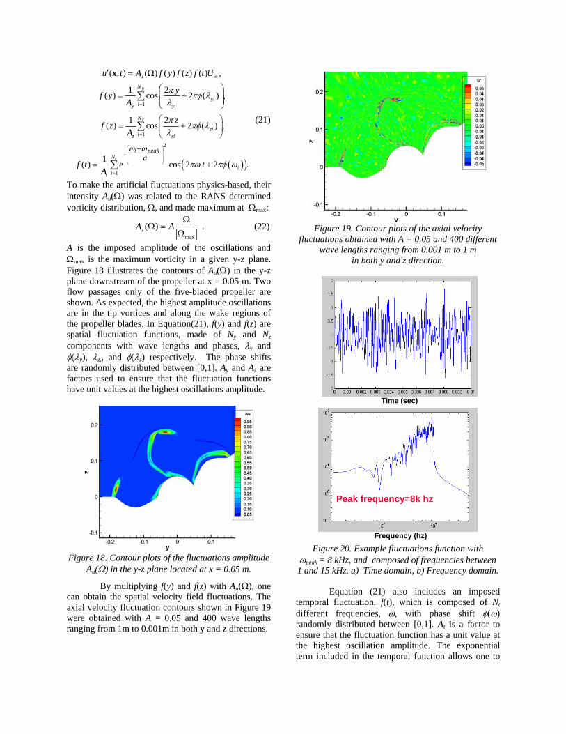
A is the imposed amplitude of the oscillations and Ωmax is the maximum vorticity in a given y-z plane. Figure 18 illustrates the contours of Au(Ω) in the y-z plane downstream of the propeller at x = 0.05 m. Two flow passages only of the five-bladed propeller are shown. As expected, the highest amplitude oscillations are in the tip vortices and along the wake regions of the propeller blades. In Equation(21), f(y) and f(z) are spatial fluctuation functions, made of Ny and Nz components with wave lengths and phases, λy and φ(λy), λz,, and φ(λz) respectively. The phase shifts are randomly distributed between [0,1]. Ay and Az are factors used to ensure that the fluctuation functions have unit values at the highest oscillations amplitude.

Figure 18. Contour plots of the fluctuations amplitude

Au(Ω) in the y-z plane located at x = 0.05 m.

By multiplying f(y) and f(z) with Au(Ω), one can obtain the spatial velocity field fluctuations. The axial velocity fluctuation contours shown in Figure 19 were obtained with A = 0.05 and 400 wave lengths ranging from 1m to 0.001m in both y and z directions.

Figure 19. Contour plots of the axial velocity

fluctuations obtained with A = 0.05 and 400 different wave lengths ranging from 0.001 m to 1 m

in both y and z direction.

Figure 20. Example fluctuations function with

ωpeak = 8 kHz, and composed of frequencies between 1 and 15 kHz. a) Time domain, b) Frequency domain.

Equation (21) also includes an imposed temporal fluctuation, f(t), which is composed of Nt different frequencies, ω, with phase shift φ(ω) randomly distributed between [0,1]. At is a factor to ensure that the fluctuation function has a unit value at the highest oscillation amplitude. The exponential term included in the temporal function allows one to

Time (sec)

Frequency (hz)

Peak frequency=8k hz

generate bias fluctuations with the highest energy centered in the specified peak frequency, ωpeak. Figure 20 illustrates an example signal composed of frequencies between 1 to 15 kHz with ωpeak = 8 kHz shown in the time and frequency domains generated.

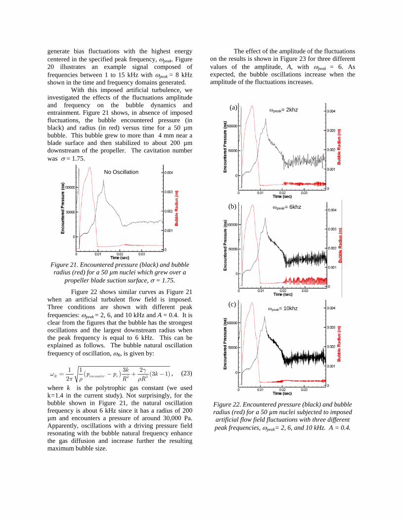
With this imposed artificial turbulence, we investigated the effects of the fluctuations amplitude and frequency on the bubble dynamics and entrainment. Figure 21 shows, in absence of imposed fluctuations, the bubble encountered pressure (in black) and radius (in red) versus time for a 50 µm bubble. This bubble grew to more than 4 mm near a blade surface and then stabilized to about 200 µm downstream of the propeller. The cavitation number was σ = 1.75.

Figure 21. Encountered pressure (black) and bubble radius (red) for a 50 µm nuclei which grew over a

propeller blade suction surface, σ = 1.75.

Figure 22 shows similar curves as Figure 21 when an artificial turbulent flow field is imposed. Three conditions are shown with different peak frequencies: ωpeak = 2, 6, and 10 kHz and A = 0.4. It is clear from the figures that the bubble has the strongest oscillations and the largest downstream radius when the peak frequency is equal to 6 kHz. This can be explained as follows. The bubble natural oscillation frequency of oscillation, ωR, is given by:

( ) ( )2 3

1 1 3 2 3 12R encounter v

kp p kR R

γωπ ρ ρ

= − + − , (23)

where k is the polytrophic gas constant (we used k=1.4 in the current study). Not surprisingly, for the bubble shown in Figure 21, the natural oscillation frequency is about 6 kHz since it has a radius of 200 µm and encounters a pressure of around 30,000 Pa. Apparently, oscillations with a driving pressure field resonating with the bubble natural frequency enhance the gas diffusion and increase further the resulting maximum bubble size.

The effect of the amplitude of the fluctuations on the results is shown in Figure 23 for three different values of the amplitude, A, with ωpeak = 6. As expected, the bubble oscillations increase when the amplitude of the fluctuations increases.

Figure 22. Encountered pressure (black) and bubble radius (red) for a 50 µm nuclei subjected to imposed artificial flow field fluctuations with three different peak frequencies, ωpeak= 2, 6, and 10 kHz. A = 0.4.

No Oscillation

ωpeak= 2khz (a)

ωpeak= 6khz (b)

ωpeak= 10khz (c)

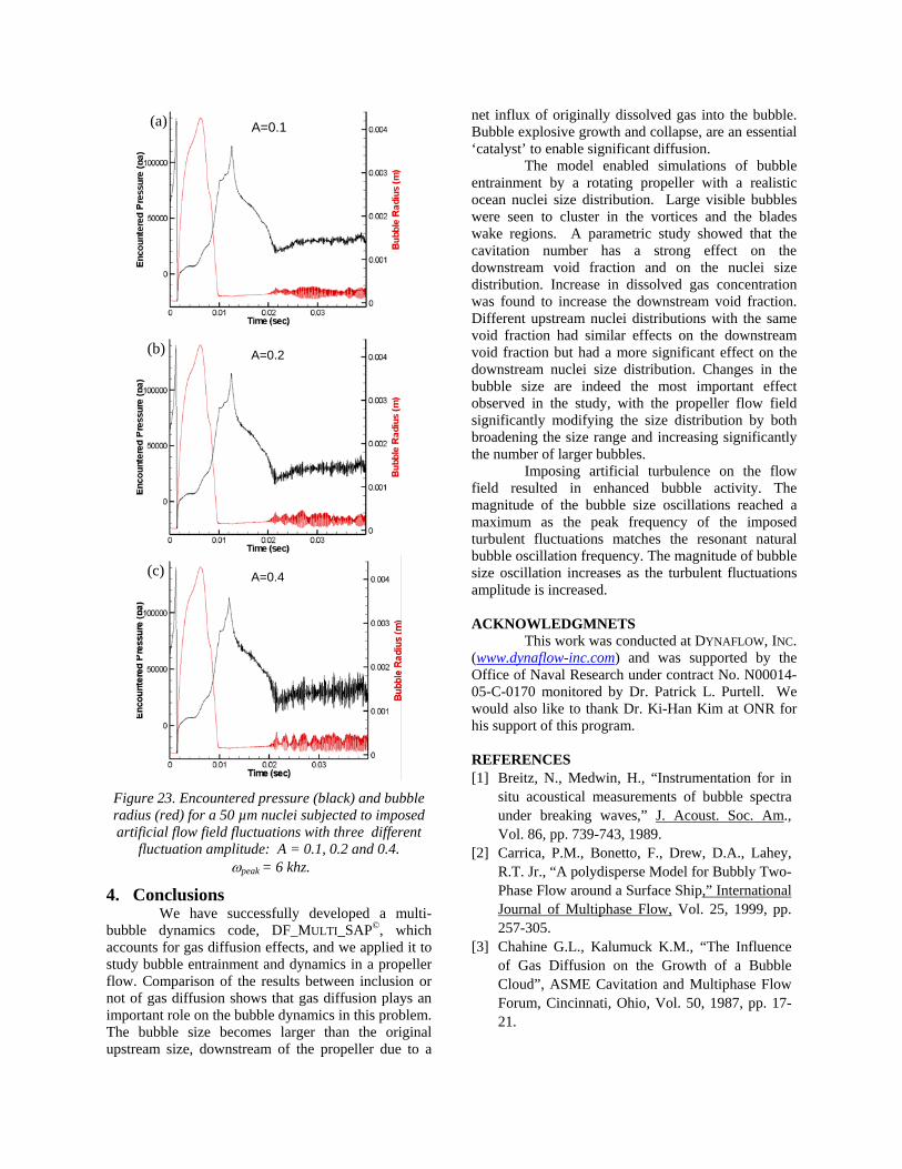
Figure 23. Encountered pressure (black) and bubble radius (red) for a 50 µm nuclei subjected to imposed artificial flow field fluctuations with three different

fluctuation amplitude: A = 0.1, 0.2 and 0.4. ωpeak = 6 khz.

4. Conclusions We have successfully developed a multi-

bubble dynamics code, DF_MULTI_SAP©, which accounts for gas diffusion effects, and we applied it to study bubble entrainment and dynamics in a propeller flow. Comparison of the results between inclusion or not of gas diffusion shows that gas diffusion plays an important role on the bubble dynamics in this problem. The bubble size becomes larger than the original upstream size, downstream of the propeller due to a

net influx of originally dissolved gas into the bubble. Bubble explosive growth and collapse, are an essential ‘catalyst’ to enable significant diffusion.

The model enabled simulations of bubble entrainment by a rotating propeller with a realistic ocean nuclei size distribution. Large visible bubbles were seen to cluster in the vortices and the blades wake regions. A parametric study showed that the cavitation number has a strong effect on the downstream void fraction and on the nuclei size distribution. Increase in dissolved gas concentration was found to increase the downstream void fraction. Different upstream nuclei distributions with the same void fraction had similar effects on the downstream void fraction but had a more significant effect on the downstream nuclei size distribution. Changes in the bubble size are indeed the most important effect observed in the study, with the propeller flow field significantly modifying the size distribution by both broadening the size range and increasing significantly the number of larger bubbles.

Imposing artificial turbulence on the flow field resulted in enhanced bubble activity. The magnitude of the bubble size oscillations reached a maximum as the peak frequency of the imposed turbulent fluctuations matches the resonant natural bubble oscillation frequency. The magnitude of bubble size oscillation increases as the turbulent fluctuations amplitude is increased.

ACKNOWLEDGMNETS

This work was conducted at DYNAFLOW, INC. (www.dynaflow-inc.com) and was supported by the Office of Naval Research under contract No. N00014-05-C-0170 monitored by Dr. Patrick L. Purtell. We would also like to thank Dr. Ki-Han Kim at ONR for his support of this program. REFERENCES [1] Breitz, N., Medwin, H., “Instrumentation for in

situ acoustical measurements of bubble spectra under breaking waves,” J. Acoust. Soc. Am., Vol. 86, pp. 739-743, 1989.

[2] Carrica, P.M., Bonetto, F., Drew, D.A., Lahey, R.T. Jr., “A polydisperse Model for Bubbly Two-Phase Flow around a Surface Ship,” International Journal of Multiphase Flow, Vol. 25, 1999, pp. 257-305.

[3] Chahine G.L., Kalumuck K.M., “The Influence of Gas Diffusion on the Growth of a Bubble Cloud”, ASME Cavitation and Multiphase Flow Forum, Cincinnati, Ohio, Vol. 50, 1987, pp. 17-21.

A=0.1 (a)

A=0.2 (b)

A=0.4 (c)

[4] Chahine G.L., Kalumuck K.M., and Perdue, T. “Cloud Cavitation and Collective Bubble Dynamics,” ONR Contract N00014-83-C-0244 Final Report. Tracor Hydronautics Technical Report 83017-1, March 1986.

[5] Chesnakas, C., Jessup, S., “Experimental Characterization of Propeller Tip Flow,” 22th Symposium on Naval Hydrodynamics, Washington, D.C., 1998, pp. 156-170.

[6] Duraiswami, R., Prabhukumar, S. and Chahine, G.L., “Bubble Counting Using an Inverse Acoustic Scattering Method”, Journal of the Acoustical Society of America, Vol. 105, No. 5, 1998.

[7] Franklin, R.E., “A note on the Radius Distribution Function for Microbubbles of Gas in Water,” ASME Cavitation and Mutliphase Flow Forum, FED-Vol. 135, 1992, pp.77-85.

[8] Gilmore, F. R., “The growth and collapse of a spherical bubble in a viscous compressible liquid,” California Institute of Technology, Hydro. Lab. Rep. 26-4, 1952.

[9] Haberman, W.L., Morton, R.K., “An Experimental Investigation of the Drag and Shape of Air Bubbles Rising in Various Liquids,” Report 802, DTMB, 1953.

[10] Hsiao, C.-T., Chahine, G.L., “Scaling of Tip Vortex Cavitation Inception Noise with a Statistic Bubble Dynamics Model Accounting for Nuclei Size Distribution”, Journal of Fluid Engineering, Vol. 127, 2005, pp. 55-64.

[11] Hsiao, C.-T., Chahine, G. L., and Liu, H.-L., “Scaling Effects on Prediction of Cavitation Inception in a Line Vortex Flow”, Journal of Fluid Engineering, Vol. 125, 2003, pp.53-60.

[12] Hsiao, C.-T., Pauley, L.L., “Numerical Computation of the Tip Vortex Flow Generated by a Marine Propeller,” ASME Journal of Fluids Engineering, Vol. 121, No. 3, 1999, pp. 638-645.

[13] Johnson, V.E., Hsieh, T., “The Influence of the Trajectories of Gas Nuclei on Cavitation Inception,” Sixth Symposium on Naval Hydrodynamics, 1966, pp. 163-179.

[14] Lord Rayleigh, On the pressure developed in a liquid during collapse of a spherical cavity, Phil. Mag; Vol. 34, 1917, pp. 94-98.

[15] MacIntyre, F., “On reconciling optical and acoustical bubble spectra in the mixed layer,” in Oceanic Whitecaps, edited by E.C. Monahan and G. Macniocaill, Reidell, New York, pp. 75-94, 1986.

[16] Oldenziel, D.M., “A new instrument in cavitation research: the cavitation susceptibility meter,” J. Fluids Engr., Vol. 104, 1982, pp. 136-142.

[17] Paterson, E.G., Hyman, M, Stern, F., Carrica, P.M., Bonetto, F., Drew, D.A., Lahey, R.T. Jr., “Near and Far-Field CFD for a Naval Combatant Including Thermal-Stratification and Two-Fluid Modeling,” 21st Symposium on Naval Hydrodynamics, Trondheim, Norway, 1996.

[18] Plesset, M. S., “Bubble Dynamics” in Cavitation in Real Liquids, Editor Robert Davies, Elsevier Publishing Company, 1964, pp. 1-17.

[19] Plesset, M.S., Zwick, S.A., “A Non-steady Heat Diffusion Problem with Spherical Symmetry,” Journal of Applied Physics, Vol. 23, No.1, 1952, pp. 95-98.

[20] Waniewski, T.A., Brennen, C.E., “Measurement of Air Entrainment by Bow Waves,” ASME Journal of Fluids Engineering, Vol. 123, 2000 pp. 57-63.